Simultaneous linear algebraic equations

Applied numerical methods lec6
Aug 14, 2015
Welcome message from author
This document is posted to help you gain knowledge. Please leave a comment to let me know what you think about it! Share it to your friends and learn new things together.
Transcript

Simultaneous linear
algebraic equations

Linear Algebraic Equations
nnnnnn
nnx
nn
bxaxaxa
bxxaeaxa
bxaxxaxa
2211
23
22223
121
15
12112111
/)()(
)(
2
nnnnnn
nn
nn
bxaxaxa
bxaxaxa
bxaxaxa
2211
22222121
11212111
Nonlinear Equations

Special Types of Square Matrices
88 6 39 16
6 9 7 2
39 7 3 1
16 2 1 5
][A
nn a
a
a
D
22
11
][
1
1
1
1
][I
Symmetric Diagonal Identity
nn
n
n
a
aa
aaa
A
][222
11211
nnn a a
aa
a
A
1
2221
11
][
Upper Triangular Lower Triangular

4
Solving Systems of Equations
• A linear equation in n variables:
a1x1 + a2x2 + … + anxn = b
• For small (n ≤ 3), linear algebra provides several tools to solve
such systems of linear equations:
– Graphical method
– Cramer’s rule
– Method of elimination
• Nowadays, easy access to computers makes the solution of
very large sets of linear algebraic equations possible

n = 2: the solution is the sole intersection point of
two lines
n = 3: each equation represents a plane in a 3D
space, and the solution is the intersection
between the three planes.
n > 3: the method fails to be of any practical use.
Manual Solutions (n ≤ 3)
12
11
12
112
a
bx
a
ax
22
21
22
212
a
bx
a
ax
The Graphical Method
Singular and ill-conditioned systems

Determinants and Cramer’s Rule
[A] : coefficient matrix BxA
3
2
1
3
2
1
333231
232221
131211
b
b
b
x
x
x
aaa
aaa
aaa
333231
232221
131211
aaa
aaa
aaa
A
D
aab
aab
aab
x33323
23222
13121
1 D
aba
aba
aba
x33331
23221
13111
2 D
baa
baa
baa
x33231
22221
11211
3
D : Determinant of A matrix
7
333231
232221
131211
aaa
aaa
aaa
D
333231
232221
131211
aaa
aaa
aaa
A
BxA
3231
2221
13
3331
2321
12
3332
2322
11A oft Determinanaa
aaa
aa
aaa
aa
aaaD
Computing the Determinant
23323322
3332
2322
11 aaaaaa
aaD
22313221
3231
2221
13
23313321
3331
2321
12
aaaaaa
aaD
aaaaaa
aaD

Manual Solutions (n ≤ 3)
An Example 1 of Cramer’s Method
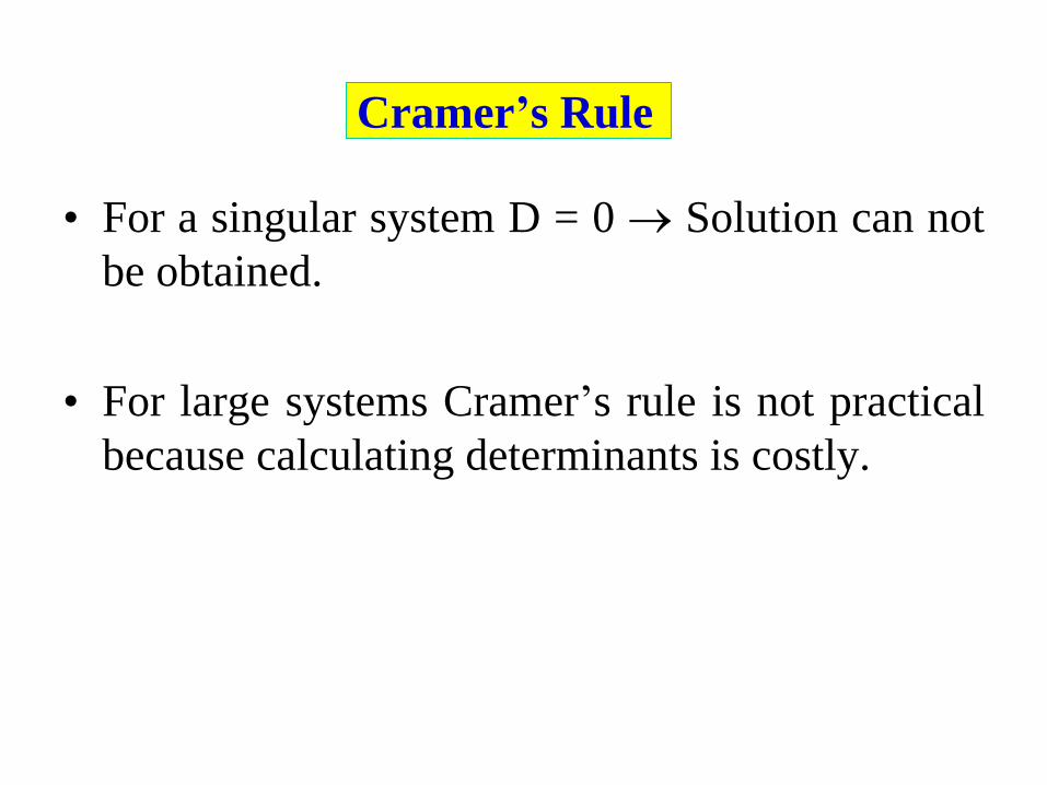
Cramer’s Rule
• For a singular system D = 0 Solution can not
be obtained.
• For large systems Cramer’s rule is not practical
because calculating determinants is costly.
10
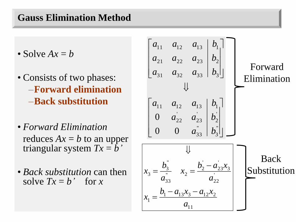
Gauss Elimination Method
• Solve Ax = b
• Consists of two phases:
–Forward elimination
–Back substitution
• Forward Elimination
reduces Ax = b to an upper triangular system Tx = b’
• Back substitution can then solve Tx = b’ for x
''
3
''
33
'
2
'
23
'
22
1131211
3333231
2232221
1131211
00
0
ba
baa
baaa
baaa
baaa
baaa
Forward
Elimination
Back
Substitution
11
21231311
'
22
3
'
23
'
22''
33
''
33
a
xaxabx
a
xabx
a
bx
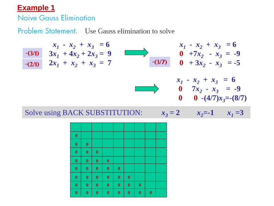
x1 - x2 + x3 = 6
3x1 + 4x2 + 2x3 = 9
2x1 + x2 + x3 = 7
x1 - x2 + x3 = 6
0 +7x2 - x3 = -9
0 + 3x2 - x3 = -5
x1 - x2 + x3 = 6
0 7x2 - x3 = -9
0 0 -(4/7)x3=-(8/7)
-(3/1)
Solve using BACK SUBSTITUTION: x3 = 2 x2=-1 x1 =3
-(2/1) -(3/7)
0
0
0
0
0
0
0
0
0
0
0
0
0
0
0
0
0
0
0
0
0
0
0
0
0
0
0
0
0
0
0
0
0
0
0 0
Example 1

Example 2


Pitfalls of Elimination Methods
Division by zero
It is possible that during both elimination and back-substitution phases a
division by zero can occur.
For example:
2x2 + 3x3 = 8 0 2 3
4x1 + 6x2 + 7x3 = -3 A = 4 6 7
2x1 + x2 + 6x3 = 5 2 1 6
Solution: pivoting (to be discussed later)

Pitfalls (cont.)
Round-off errors
• A round-off error, also called rounding error, is the difference between the
calculated approximation of a number and its exact mathematical value.
• Because computers carry only a limited number of significant figures,
round-off errors will occur and they will propagate from one iteration to the
next.
• This problem is especially important when large numbers of equations (100
or more) are to be solved.
• Always use double-precision numbers/arithmetic. It is slow but needed for
correctness!
• It is also a good idea to substitute your results back into the original
equations and check whether a substantial error has occurred.
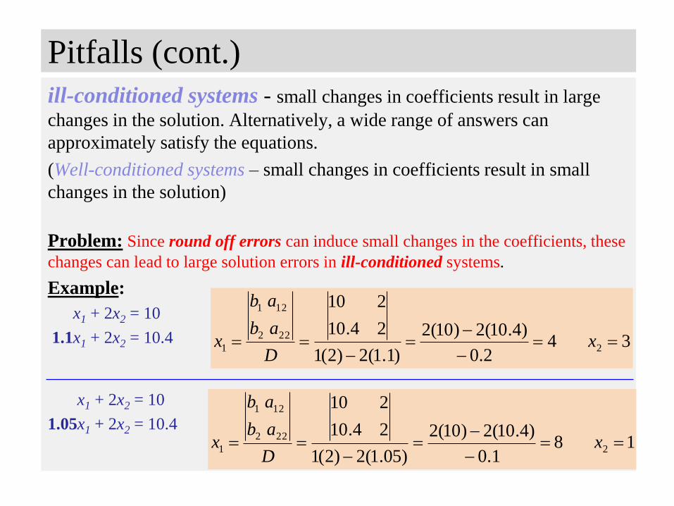
ill-conditioned systems - small changes in coefficients result in large
changes in the solution. Alternatively, a wide range of answers can
approximately satisfy the equations.
(Well-conditioned systems – small changes in coefficients result in small
changes in the solution)
Problem: Since round off errors can induce small changes in the coefficients, these
changes can lead to large solution errors in ill-conditioned systems.
Example:
x1 + 2x2 = 10
1.1x1 + 2x2 = 10.4
x1 + 2x2 = 10
1.05x1 + 2x2 = 10.4
3 42.0
)4.10(2)10(2
)1.1(2)2(1
2 4.10
2 10
2
222
121
1
x
D
ab
ab
x
1 81.0
)4.10(2)10(2
)05.1(2)2(1
2 4.10
2 10
2
222
121
1
x
D
ab
ab
x
Pitfalls (cont.)

• Surprisingly, substitution of the wrong values, x1=8 and x2=1, into the original equation will not reveal their incorrect nature clearly:
x1 + 2x2 = 10 8+2(1) = 10 (the same!)
1.1x1 + 2x2 = 10.4 1.1(8)+2(1)=10.8 (close!)
IMPORTANT OBSERVATION:
An ill-conditioned system is one with a determinant close to zero
• If determinant D=0 then there are infinitely many solutions singular system
• Scaling (multiplying the coefficients with the same value) does not change the equations but changes the value of the determinant in a significant way.
However, it does not change the ill-conditioned state of the equations!
DANGER! It may hide the fact that the system is ill-conditioned!!
How can we find out whether a system is ill-conditioned or not?Not easy! Luckily, most engineering systems yield well-conditioned results!
• One way to find out: change the coefficients slightly and recompute & compare
ill-conditioned systems (cont.) –
19
COMPUTING THE DETERMINANT OF A MATRIX
USING GAUSSIAN ELIMINATION
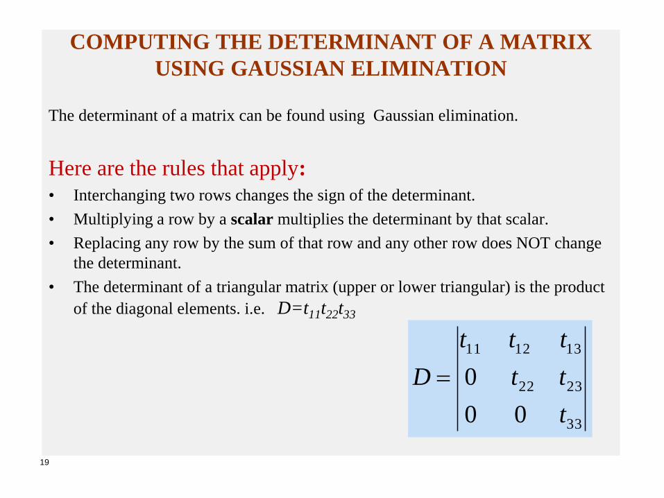
The determinant of a matrix can be found using Gaussian elimination.
Here are the rules that apply:
• Interchanging two rows changes the sign of the determinant.
• Multiplying a row by a scalar multiplies the determinant by that scalar.
• Replacing any row by the sum of that row and any other row does NOT change
the determinant.
• The determinant of a triangular matrix (upper or lower triangular) is the product
of the diagonal elements. i.e. D=t11t22t33
33
2322
131211
00
0
t
tt
ttt
D
Techniques for Improving Solutions
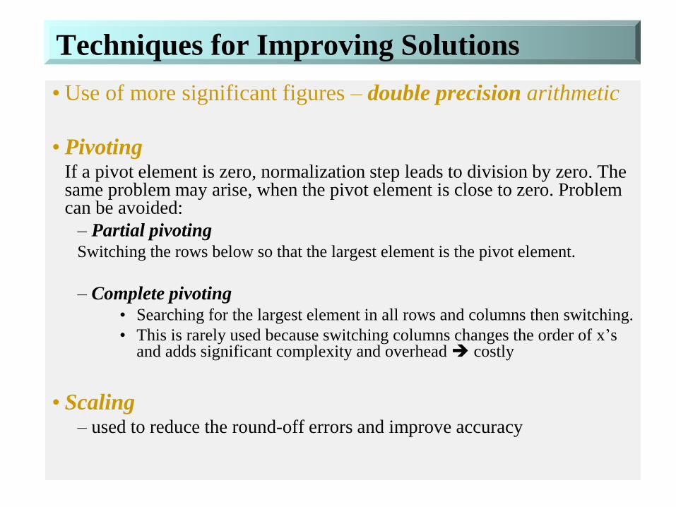
• Use of more significant figures – double precision arithmetic
• PivotingIf a pivot element is zero, normalization step leads to division by zero. The same problem may arise, when the pivot element is close to zero. Problem can be avoided:
– Partial pivotingSwitching the rows below so that the largest element is the pivot element.
– Complete pivoting• Searching for the largest element in all rows and columns then switching.
• This is rarely used because switching columns changes the order of x’sand adds significant complexity and overhead costly
• Scaling– used to reduce the round-off errors and improve accuracy

Pivoting
• Consider this system:
• Immediately run into problem:
algorithm wants us to divide by zero!
• More subtle version:
8
2
32
10
8
2
32
1001.0
Pivoting
• Conclusion: small diagonal elements bad
• Remedy: swap in larger element from
somewhere else

Partial Pivoting
• Swap rows 1 and 2:
• Now continue:
8
2
32
10
2
8
10
32
2
1
10
01
2
4
10
1 23

Full Pivoting
• Swap largest element onto diagonal by
swapping rows 1 and 2 and columns 1 and 2:
• Critical: when swapping columns, must
remember to swap results!
8
2
32
10
2
8
01
23
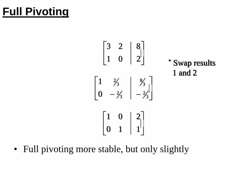
Full Pivoting
• Full pivoting more stable, but only slightly
2
8
01
23
32
38
32
32
0
1
1
2
10
01
* Swap results
1 and 2

Example 3: Gauss Elimination
2 4
1 2 3 4
1 2 4
1 2 3 4
2 0
2 2 3 2 2
4 3 7
6 6 5 6
x x
x x x x
x x x
x x x x
a) Forward Elimination
0 2 0 1 0 6 1 6 5 6
2 2 3 2 2 2 2 3 2 21 4
4 3 0 1 7 4 3 0 1 7
6 1 6 5 6 0 2 0 1 0
R R

Example 3: Gauss Elimination (cont’d)
6 1 6 5 6
2 2 3 2 2 2 0.33333 1
4 3 0 1 7 3 0.66667 1
0 2 0 1 0
6 1 6 5 6
0 1.6667 5 3.6667 42 3
0 3.6667 4 4.3333 11
0 2 0 1 0
6 1 6 5 6
0 3.6667 4 4.3333 11
0 1.6667 5 3.6667 4
0 2 0 1 0
R R
R R
R R

Example 3: Gauss Elimination (cont’d)
6 1 6 5 6
0 3.6667 4 4.3333 11
0 1.6667 5 3.6667 4 3 0.45455 2
0 2 0 1 0 4 0.54545 2
6 1 6 5 6
0 3.6667 4 4.3333 11
0 0 6.8182 5.6364 9.0001
0 0 2.1818 3.3636 5.9999 4 0.32000 3
6 1 6
0 3.6667 4
0 0 6.8
0 0
R R
R R
R R
5 6
4.3333 11
182 5.6364 9.0001
0 1.5600 3.1199
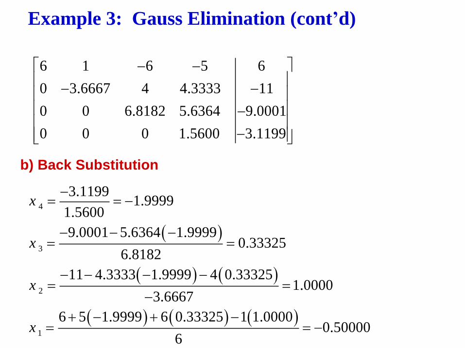
Example 3: Gauss Elimination (cont’d)
b) Back Substitution
6 1 6 5 6
0 3.6667 4 4.3333 11
0 0 6.8182 5.6364 9.0001
0 0 0 1.5600 3.1199
4
3
2
1
3.11991.9999
1.5600
9.0001 5.6364 1.99990.33325
6.8182
11 4.3333 1.9999 4 0.333251.0000
3.6667
6 5 1.9999 6 0.33325 1 1.00000.50000
6
x
x
x
x


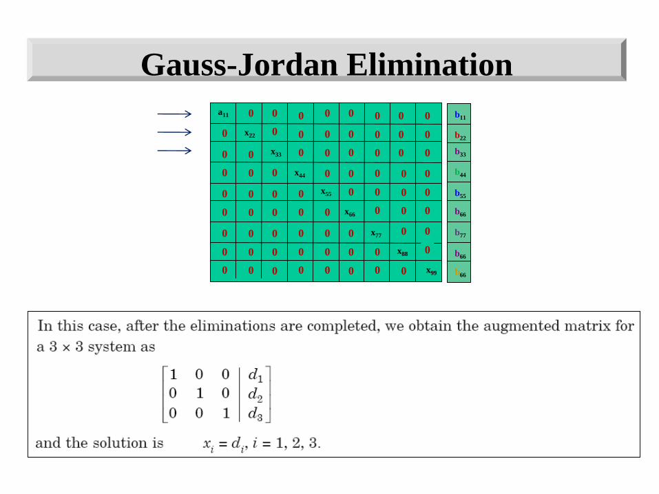
Gauss-Jordan Elimination
0
0
0
0
0
0
0
0
0
0
0
0
0
0
0
0
0
0
0
0
0
0
0
0
0
0
0
0
0
0
0 0
0
a11
x22
0
x33
0
0
x44
0
0
0
x55
0
0
0
0
x66
x77
x88
0
0
0
0
0
0
0
0
0
0
0
0
0
0
0
0
0
0
0
0
0
0
0
0
0
0
b11
b22
b33
b44
b55
b66
b77
b66
b660 0 0 x99

Gauss-Jordan Elimination: Example 4
10
1
8
|
|
|
473
321
211
:Matrix Augmented
10
1
8
473
321
211
3
2
1
x
x
x
1 1 2 | 8
0 1 5 | 9
0 4 2| 14
R2 R2 - (-1)R1
R3 R3 - ( 3)R1
Scaling R2:
R2 R2/(-1)
R1 R1 - (1)R2
R3 R3-(4)R2
1 1 2 | 8
0 1 5| 9
0 4 2| 14
22
9
17
|
|
|
1800
510
701
Scaling R3:
R3 R3/(18)
9/11
9
17
|
|
|
100
510
701
222.1
888.2
444.8
|
|
|
100
010
001
R1 R1 - (7)R3
R2 R2-(-5)R3
RESULT:
x1=8.45, x2=-2.89, x3=1.23
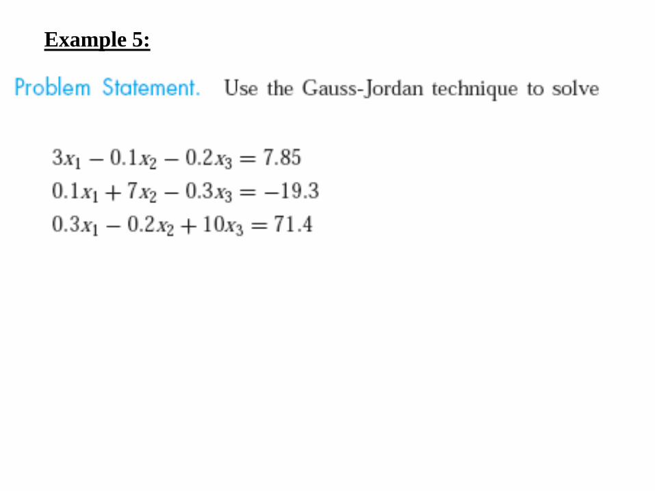
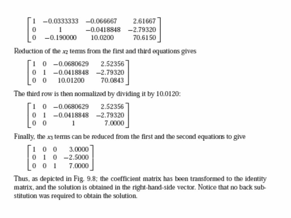
Example 5:


Motivation
• The elimination method becomes inefficient when solving
equations with the same coefficients [A] but different right-
hand-side constants (the b’s).
• The LU decomposition also provides an efficient means to
compute the matrix inverse.
• Gauss elimination itself can be expressed as an LU
decomposition.
BXA
The LU decomposition method

Example 6:

Notice that for the LU decomposition implementation of Gauss elimination, the [L]
matrix has 1’s on the diagonal. This is formally referred to as a Doolittle
decomposition, or factorization. An alternative approach involves a [U] matrix with
1’s on the diagonal. This is called Crout decomposition.
333231
232221
131211
aaa
aaa
aaa
A
[ U ][ L ]
33
2322
131211
3231
21
00
0
1
01
001
u
uu
uuu
ll
l
upper triangular
matrix
lower triangular
matrix

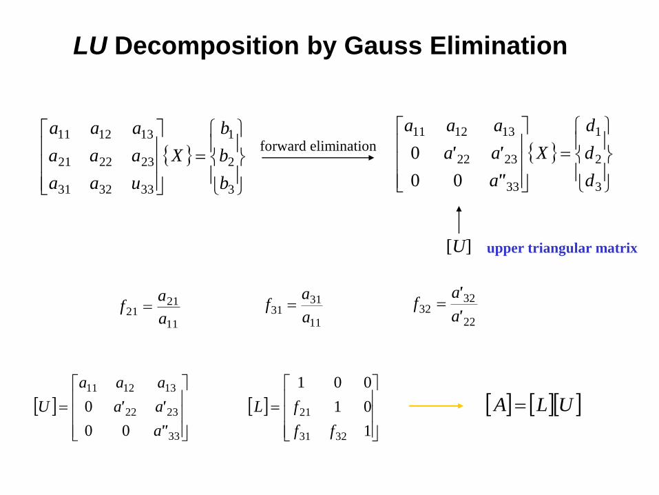
LU Decomposition by Gauss Elimination
3
2
1
33
2322
131211
00
0
d
d
d
X
a
aa
aaa
"
''
3
2
1
333231
232221
131211
b
b
b
X
uaa
aaa
aaa
22
3232
'
'
a
af
forward elimination
[U]
11
2121
a
af
11
3131
a
af
33
2322
131211
00
0
"
''
a
aa
aaa
U
1
01
001
3231
21
ff
fL ULA
upper triangular matrix

22
3232
'
'
a
af
11
2121
a
af
11
3131
a
af
U =
33
2322
131211
00
0
"
''
a
aa
aaa
U
Example 6 (cont’d):

Example 6 (cont’d):

Example 6 (cont’d):
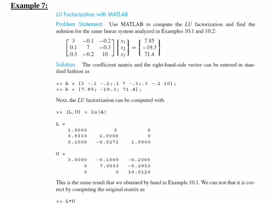
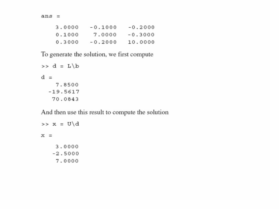
Example 7:

CW 1: Use the LU decomposition method to solve


CW 2: Use the LU decomposition method to solve


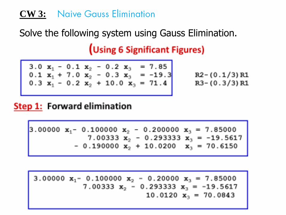
CW 3:
Solve the following system using Gauss Elimination.


Jacobi Iterative Method
])([ )( )]([
xDAbDxxDAbDxbxDAD
a
a
a
D
aaa
aaa
aaa
AbAx
1
33
22
11
333231
232221
131211
00
00
00
33
1
232
1
13133
22
1
323
1
12122
11
1
313
1
21211
a
xaxabx
a
xaxabx
a
xaxabx
kkk
kkk
kkk
*
/
/
/
3
2
1
3231
2321
1312
3
2
1
33
22
11
3
2
1
0
0
0
100
010
001
x
x
x
aa
aa
aa
b
b
b
a
a
a
x
x
x
Choose an initial guess (i.e. all zeros) and Iterate until the equality is satisfied.
No guarantee for convergence!
Iterative methods provide an alternative to the elimination
methods.

Gauss-Seidel Iteration Method
• The Gauss-Seidel method is a commonly used iterative method.
• It is same as Jacobi technique except with one important difference:
A newly computed x value (say xk) is substituted in the subsequent equations (equations k+1, k+2, …, n) in the same iteration.
Example: Consider the 3x3 system below:
• First, choose initial guesses for the x’s.
• A simple way to obtain initial guesses is
to assume that they are all zero.
• Compute new x1 using the previous
iteration values.
• New x1 is substituted in the equations to
calculate x2 and x3
• The process is repeated for x2, x3, …newold
newnewnew
oldnewnew
oldoldnew
XX
a
xaxabx
a
xaxabx
a
xaxabx
}{}{
33
23213133
22
32312122
11
31321211
56
Convergence Criterion for Gauss-Seidel Method
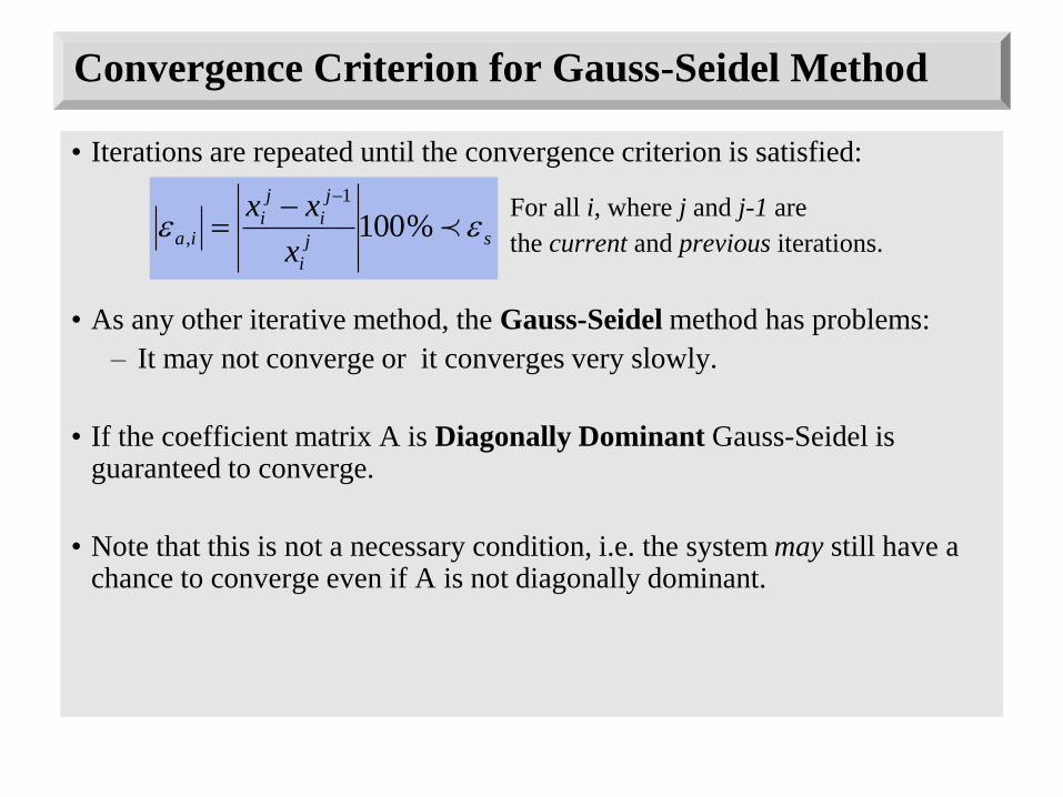
• Iterations are repeated until the convergence criterion is satisfied:
For all i, where j and j-1 are
the current and previous iterations.
• As any other iterative method, the Gauss-Seidel method has problems:
– It may not converge or it converges very slowly.
• If the coefficient matrix A is Diagonally Dominant Gauss-Seidel is guaranteed to converge.
• Note that this is not a necessary condition, i.e. the system may still have a chance to converge even if A is not diagonally dominant.
sj
i
j
i
j
iia
x
xx %100
1
,

57
newold
newnewnew
oldnewnew
oldoldnew
XX
a
xaxabx
a
xaxabx
a
xaxabx
}{}{
33
23213133
22
32312122
11
31321211
Example 8 (Gauss-Seidel Method) :


Special Problem 4

Home Work 2
1.

2.
3.

4.
5. Use Gauss-Seidel method to solve the system
Related Documents