Applied Nonlinear Optics David C. Hutchings Dept. of Electronics and Electrical Engineering University of Glasgow

Welcome message from author
This document is posted to help you gain knowledge. Please leave a comment to let me know what you think about it! Share it to your friends and learn new things together.
Transcript

Applied Nonlinear Optics
David C. HutchingsDept. of Electronics and Electrical Engineering
University of Glasgow

ii

Preface
This course will cover aspects of birefringence, the electro-optic effect and optical frequencyconversion. It will be necessary to have a good grounding in electro-magnetic theory and opticsprior to this course. Recommended textbooks for this material are Shen [1], Zernike and Mid-winter [2] and Yariv [3]. Like the bulk of the literature in nonlinear optics, these books do notalways employ a consistent SI notation. I would recommend Butcher and Cotter [4], althoughnot as applied as the above references, for its consistent notation (SI units) and formalism.
iii

iv

Chapter 1
Birefringence
1.1 Dielectrics (revision)
In a vacuum, Gauss’ theorem states that the closed surface integral of the normal component ofthe electric field to the surface is proportional to the total charge enclosed by the surface,
∫E ·ds= ∑ q
ε0=
1ε0
∫ρdV , (1.1)
whereρ is the charge density. The divergence theorem can be used to change this surfaceintegral to a volume integral, ∫
E ·ds=∫
∇ ·EdV , (1.2)
which allows us to relate two volume integrals. Now since these are over the same region whichwe can arbitrarily choose, the integrands must be equal, i.e.,
∇ ·E =ρε0
. (1.3)
Hence we have used the divergence theorem to transform the original integral equation [Eq.(1.1)] for the electric field into a differential one.
Let us now address the issue of an electric field in a dielectric medium. The electric fieldwill induce dipoles in the medium, for example by distortion of the electron clouds or aligningpolar molecules preferentially along the direction of the field. In an extended medium anda uniform field the average charge density due to these induced dipoles is zero except at thesurfaces. This is because the charge on one end of an induced dipole will be neutralised bythe opposite charge on the end of an adjacent dipole. At the surface there is no adjacent dipoleto cancel the charge. Thus additional polarisation charges have been generated at the surfacewhich must be accounted for. Similar polarisation charges are generated in the case of a non-uniform field. A polarisation fieldP can be defined equal to the dipole moment per unit volume.If there areN dipoles per unit volume consisting of charges+q and−q separated byr then
1

2 CHAPTER 1. BIREFRINGENCE
P = Nqr . If we assume for a moment that the induced charge separationr ∝ E,1 then thepolarisation field is proportional and parallel to the electric field. Conventionally this is writtenin SI units asP = ε0χE, where the dimensionless constant of proportionalityχ is called theoptical susceptibility.
It can be shown that the effective charge density due to the polarisation of a medium is givenby, ρp =−∇ ·P. Inserting this into the differential form of Gauss’ theorem gives,
∇ ·E =1ε0
(ρ+ρp) =1ε0
(ρ−∇ ·P) , (1.4)
whereρ denotes the free (not polarisation) charge density. This can be rearranged to give∇ · (ε0E+P) = ρ. For convenience a new field is introduced at this point equal to the quantityinside the bracket,D = ε0E+P, conventionally known as the electric displacement. Note thatunlike E andP the electric displacement is not immediately related to a physical quantity, butallows various electro-magnetic relations to be written in a far simpler form. However,D canbe thought of as a vacuum field, consisting of the contribution to the electric field with the effectof the dielectric medium subtracted. The simpler form of Eq. (1.4) is∇ ·D = ρ and is one of theset of differential relations known as Maxwell’s equations. Using the susceptibility to substitutefor the polarisation field provides,
D = ε0(1+χ)E = ε0εrE , (1.5)
whereεr = 1+ χ is known as the dielectric constant or relative permittivity. Note that thevacuum values of these dimensionless quantities areχ = 0 andεr = 1.
The divergence theorem and Stokes theorem are employed in deriving the remainder ofMaxwell’s equations. We shall state these without proof here as we will be making frequent useof them throughout this course. In SI units they are given by:
∇ ·D = ρ ,
∇ ·B = 0 ,
∇×E = −∂B∂t
,
∇×H = j +∂D∂t
.
The current is related to the electric field by the conductivity,j = σE. In this course the usualcase will be of zero currentj = 0 and non-magnetic materialB = µ0H.
1.2 The Dielectric Tensor
In an anisotropic media the dipoles may be constrained so their direction is different to that ofthe electric field. One can think of numerous mechanical analogies where the motion of a mass
1This corresponds to the simplest case of a medium which is linear and isotropic. Most of the course considersthe extension of this to cases where the two vectors are (i) not parallel or (ii) not simply proportional.

1.2. THE DIELECTRIC TENSOR 3
is constrained by e.g. ramps or string so that acceleration is not parallel to the force. In suchsystems, the constraint reduces the symmetry. If the dipoles are not parallel to the field, thenthe polarisationP and the electric displacementD are also not parallel to the fieldE. HenceEq. (1.5) cannot be written with the relative permittivity as a scaler quantity. To generalise Eq.(1.5) to anisotropic media (such thatD andE can have different directions), the scaler dielectricconstantεr is replaced with a second rank tensor,
1ε0
Dx
Dy
Dz
=
εxx εxy εxz
εyx εyy εyz
εzx εzy εzz
Ex
Ey
Ez
. (1.6)
In a more compact notation,1ε0
Di = ∑j=x,y,z
εi j E j . (1.7)
We can prove that the tensorεi j is symmetric using energy conservation. The energy densityof an electric field in a dielectric is,
We =12
E ·D =12∑
i, jEiεi j E j . (1.8)
Differentiating gives the power flow into a unit volume,
∂We
∂t=
12∑
i jεi j
(∂Ei
∂tE j +Ei
∂E j
∂t
). (1.9)
We can also calculate power flow using the Poynting vector which is the power flow across aunit area,S= E×H. Using the divergence theorem gives the power flow per unit volume,
∇ ·S= ∇ · (E×H) = E ·∇×H−H ·∇×E . (1.10)
We can substitute for the vector curls using Maxwell’s equations and assuming no currentsj = 0gives a power flow per unit volume,
E · ∂D∂t
+H · ∂B∂t
. (1.11)
The first of these terms relates to the rate of change of energy of the electric field,
∂We
∂t= E · ∂D
∂t= ∑
i jεi j Ei
∂E j
∂t. (1.12)
Now these two forms of power flow must be the same and hence Eqs. (1.9) and (1.12) must beequal. This can only be the case ifε ji = εi j and the dielectric tensor is symmetric having a totalof 6 different elements.
Note that we have not yet specified the axes for our cartesian co-ordinate systemx,y,z. Itis always possible to choose a set such that the (symmetric) dielectric tensor is diagonal. The

4 CHAPTER 1. BIREFRINGENCE
basis of this is that a symmetric matrix is specific case of a Hermitian matrix and has pure realeigenvalues and eigenvectors. Thus if we change to a new co-ordinate system where the axesare parallel to these eigenvectors, the dielectric tensor becomes diagonal,
1ε0
Dx
Dy
Dz
=
εx 0 00 εy 00 0 εz
Ex
Ey
Ez
, (1.13)
whereεx = εxx etc. The set of axes in this case is known as the principal dielectric axes, whichmay be different from the usual crystal axes.
The dielectric tensor may be further simplified by considering the crystal symmetry. Thereare three distinctive cases summarised in table 1.1. It can be seen that generally the higherthe degree of symmetry, the lower the degree of birefringence. In most of the above crystalsystems the principal dielectric axes correspond to the usual cartesian crystalline axes. The twoexceptions to this are the monoclinic and triclinic crystal systems.
No birefringence IsotropicCubic
ε 0 00 ε 00 0 ε
Uniaxial birefringence(1 optic axis)
HexagonalTetragonalTrigonal
εx 0 00 εx 00 0 εz
Biaxial birefringence(2 optic axes)
OrthorhombicMonoclinicTriclinic
εx 0 00 εy 00 0 εz
Table 1.1: The form of the dielectric tensor for the various crystal symmetries indicated.
1.3 EM Wave propagation
Now consider the propagation of a monochromatic electro-magnetic plane wave through themedium. Such a wave has electric and magnetic fields given by,
E =12
[E0e−i(ωt−k·r) +E∗0ei(ωt−k·r)
], (1.14)
H =12
[H0e−i(ωt−k·r) +H∗
0ei(ωt−k·r)]
. (1.15)
The wavevectork = nωs/c wheres is a unit vector in the direction of propagation of the wave.The phase velocity is given byvp = cs/n. Inserting these into Maxwell’s equation∇×E =

1.3. EM WAVE PROPAGATION 5
−∂B/∂t with a nonmagnetic medium (B = µ0H) gives,
H0 =1
ωµ0k×E0 =
nµ0c
s×E0 . (1.16)
Thus the direction of the magnetic field amplitude is perpendicular to both the direction ofpropagations and electric fieldE0. Similarly we can use the Maxwell equation∇×H = j +∂D/∂t with j = 0 to obtain,
D0 =− 1ω
k×H0 =−nc
s×H0 . (1.17)
Hence the electric displacement is perpendicular to the direction of propagations and the mag-netic fieldH0. However, as we have seen for anisotropic media,E0 andD0 are not necessarilyparallel. We also note that the power flow is given by the Poynting vectorS = E×H whichis perpendicular toE0 andH0. The Poynting vector also provides the direction for the groupvelocity. Fig. 1.1 shows the relative geometry of these vectors in an anisotropic medium. Thisillustrates that the propagation directions and the Poynting vector are not necessarily paralleland hence the phase and group velocities may also not be parallel.
E D
S=ExH
k
v
v
g
p
H
Figure 1.1: Relative geometry of the field vectors and the phase and group velocities for anem-wave in an anisotropic medium. The magnetic fieldH is directed out of the page.
Combining Eqs. (1.16) and (1.17) gives,
D0 =− n2
µ0c2 s× s×E0 = n2ε0 [E0− s(s·E0)] . (1.18)
Consider just one component of this expression and introduce the dielectric tensor,
D0i = n2[
D0i
εi− ε0si (s·E0)
],
D0i = ε0si (s·E0)(
1εi− 1
n2
)−1
. (1.19)

6 CHAPTER 1. BIREFRINGENCE
SinceD0 ands are perpendicular,D0 · s= 0. This provides the relation,
∑i
s2i
(n2
εi−1
)−1
= 0 , (1.20)
which is known as Fresnel’s equation. This is quadratic in the square of the refractive index (n2)and therefore provides two possible solutions given a propagation directions. Hence the originof the name of this phenomenon; birefringence which means literally double refraction.
It can be shown that these two roots for the refractive index correspond to orthogonal po-larisations. Let the two roots ben′ andn′′ with electric displacement amplitudesD′0 andD′′0respectively. Using Eq. (1.19), the scaler product of these amplitudes can be written,
D′0 ·D′′0 =(ε0n′n′′s·E0
)2∑i
s2i
(n′2/εi−1)(n′′2/εi−1),
=(ε0n′n′′s·E0)
2
n′′2−n′2 ∑i
(n′2
n′2/εi−1− n′′2
n′′2/εi−1
)s2i , (1.21)
where partial fractions have been employed to obtain the final form. Now Fresnel’s equation(1.20) states that the summation over each of the terms is zero. HenceD′0 ·D′′0 = 0 and therforeD′0 andD′′0 are mutually perpendicular.
1.4 The Index Ellipsoid
Using Fresnel’s equation based on the propagation direction is rather cumbersome when analys-ing birefringence. A much easier method is based on the direction of the electric displacement.The energy density of an electric field in a birefringent dielectric is,
We =12
E ·D =12
(D2
x
εx+
D2y
εy+
D2y
εy
). (1.22)
Substitutingεr = n2 for the various directions and settingDx/√
2We= x, etc. gives the following,
x2
n2x+
y2
n2y+
z2
n2z
= 1 . (1.23)
This equation represents an ellipsoid and is conventionally referred to as the index ellipsoid oroptical indicatrix. The intercepts of this surface with the cartesian axes are at±nx for thex-axis,etc. This ellipsoid can be used to find the two allowed directions for the polarisation and theirassociated refractive indices.
The remaining discussion will focus on uniaxial birefringence whereny = nx. This meansthat the index ellipsoid will have cylindrical symmetry round thez-axis (optic axis). There aretwo distinct cases of uniaxial birefringence;nz > nx known as positive unixial birefringence and

1.4. THE INDEX ELLIPSOID 7
nz < nx known as negative unixial birefringence. These are illustrated in Fig. 1.2. The use ofthe index ellipsoid is as follows. The direction of propagationk is drawn from the origin andmakes an angle ofθ to the optic axis. The intersection of the plane normal to the direction ofpropagation and the index ellipsoid generates an ellipse with semi-axesa andb. For a uniaxialcrystal, the semi-axisa (minor semi-axis in the case of a positive uniaxial crystal, major semi-axis in the case of a negative uniaxial crystal) always lies in thexy-plane and therefore has alengtha = nx = no independent of the angleθ; a ray with this polarisation is called the ordinaryray. The length of the other semi-axis is dependent on the angleθ, b = ne(θ); a ray withthis polarisation is called the extraordinary ray. When the direction of propagation is parallelor perpendicular to the optic axis, the refractive index of the extraordinary ray can be writtendown immediately,ne(θ = 0) = nz = ne andne(θ = π/2) = nx = no. For the general case, wedecomposeb = ne(θ) into components parallel and perpendicular to the optic axis,x2 + y2 =(ne(θ)cosθ)2 andz= ne(θ)sinθ, and insert into the equation for the index ellipsoid to give foruniaxial crystals,
1n2
e(θ)=
cos2θn2
o+
sin2θn2
e. (1.24)
z
x
k
θ
b
a
(a) (b)z
x
zz xn >n n <nx
Figure 1.2: The index ellipsoid or optical indicatrix for (a) a positive uniaxial crystal and (b) anegative uniaxial crystal. They-axis is directed into the page.
If we re-examine the derivation of Eq. (1.19), it can be seen that ifn2 = εi for i = x, y or zthens·E0 = 0 and the electric field amplitudeE0 is perpendicular to the propagation directionand hence parallel to the electric displacement amplitudeD0. For the ordinary ray in a uniaxialcrystal this is satisfied for any propagation direction sincen2
0 = εx = εy. Hence the derivationof the term ordinary since the phase and group velocities are parallel as in a non-birefringentmedium. For the extraordinary ray, this condition only occurs for propagation parallel or per-pendicular to the optic axis. In general, the phase and group velocities are not parallel.
Calcite (crystalline calcium carbonate) is a common uniaxial birefringent crystal and is use-ful in demonstrating the properties of birefringence. Place a piece of calcite over a piece of

8 CHAPTER 1. BIREFRINGENCE
paper with text on it and you will see a double image. If you have a polariser, place it over thecalcite and rotate it. You should find at some point that only one image will be visible. Rotatethe polariser by 90 and only the other image will be visible. This demonstrates that the twoimages correspond to orthogonal polarisations. Now remove the polariser and rotate the calcite.You should find that one of the images remains stationary and the other rotates about it. The sta-tionary image corresponds to the ordinary ray where the phase and group velocities are paralleland correspondingly the rotating image corresponds to the extraordinary ray.
1.5 Wave Plates
So far we have only considered light to be exclusively of ordinary or extraordinary polarisa-tion. What happens in the general case where the light is some combination of these po-larisation states? Suppose we initially have a linear polarisationDin
0 = D0(ocosφ + esinφ)where o and e are unit vectors parallel to the ordinary and extraordinary polarisation direc-tions respectively. Now suppose the crystal thicknessd is such that the difference in opticalpath length between the ordinary and extraordinary rays is an odd integer of half-wavelengths(ne(θ)−no)d = (2N +1)λ/2. A crystal of this thickness is termed a half-wave plate. On exitthe ordinary and extraordinary rays will be out of phase,Dout
0 = D0(ocosφ− esinφ).2 It canbe seen that this is equivalent to the transformφ →−φ and corresponds to flipping the polar-isation angle around the optic axis. In particular forφ = 45, the output (linear) polarisation isperpendicular to the input.
Now let us consider a crystal of thickness such that the optical path length difference is anodd number of quarter wave-lengths(ne(θ)− no)d = (2N + 1)λ/4 known as a quarter waveplate. Now the ordinary and extraordinary rays will beπ/2 out of phase with each other onoutput from the crystal. Again if we consider the particular case of an input linear polarisationat 45 to the optic axisDin
0 = D0(o− e)/√
2 then the output polarisation will beDout0 = D0(o±
ie)/√
2. The positive and negative cases correspond to the separate cases ofNλ + λ/4 andNλ +3λ/4 optical path length differences. In this case we have generated circularly polarisedlight from a linearly polarised input. A quarter wave plate can also perform the reverse, changingcircularly polarised light to linear (since two consecutive quarter wave plates make a half waveplate).
2For simplicity the common phase factor has been omitted since the polarisation state only depends on therelative phase of the polarisation components

Chapter 2
The Electro-optic Effect
2.1 The Electro-optic tensor
The change in refractive index with a DC electric field is known as the electro-optic effect. Inthis chapter we will consider the linear electro-optic effect or Pockel’s effect where∆n ∝ E.There also exists the quadratic electro-optic effect or Kerr effect which is associated with higherorder effects considered later in this course. The principal application of the electro-optic effectis in optical modulators where we use an external influence (applied voltage) to change theoptical properties of a material.
The general form of the optical indicatrix if the axes do not necessarily correspond to theprincipal dielectric axes is,
x2
εxx+
y2
εyy+
z2
εzz+
2yzεyz
+2xzεxz
+2xyεxy
= 1 , (2.1)
or in shorthand notation,∑i, j=x,y,zi jεi j
= 1. Now conventionally the electro-optic coefficientr
relates the change in1/ε (i.e. 1/n2) to the electric fieldE. Generalising this to anisotropiccrystals,
∆(
1εi j
)=
(1
εi j
)
E−
(1
εi j
)
E=0= ∑
k
r i jkEk . (2.2)
The electro-optic coefficientr i jk is a third rank tensor as it relates a second rank tensor (1/εi j )to a vector (E). It has 27 elements but only 18 are independent sinceε ji = εi j and thereforer jik = r i jk . This symmetry is employed to write the electro-optic tensor in a contracted notationwhere thei j subscripts are replaced by:xx= 1, yy= 2, zz= 3, yz= zy= 4, xz= zx= 5 andxy= yx= 6 and thek subscripts by:x = 1, y = 2 andz= 3. This allows the electro-optic tensor
9

10 CHAPTER 2. THE ELECTRO-OPTIC EFFECT
to be written as a6×3 matrix:
∆(1/ε1)∆(1/ε2)∆(1/ε3)∆(1/ε4)∆(1/ε5)∆(1/ε6)
=
r11 r12 r13
r21 r22 r23
r31 r32 r33
r41 r42 r43
r51 r52 r53
r61 r62 r63
E1
E2
E3
. (2.3)
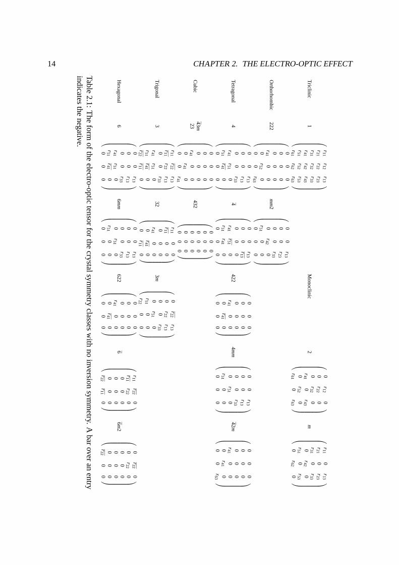
As in the case of the dielectric tensor, symmetry considerations provide information as towhich electro-optic coefficient tensor elements are non-zero and independent. An importantproperty is that materials with inversion symmetry exhibit no electro-optic effect. Consider Eq.(2.2) under the application of the inversion operator. If the material has inversion symmetry thenthe material parametersεi j andr i jk are unchanged. However, under inversionEk→−Ek. Hence∑k r i jkEk =−∑k r i jkEk for any specifiedE which requires that all the electro-optical coefficientsare zero,r i jk = 0. For other symmetry classes, group theory can be employed to investigate theform of the electro-optic tensor, as shown in table 2.1.
2.2 Examples
2.2.1 KDP
Potassium dihydrogen phosphate KH2PO4 (known as KDP) belongs to the symmetry class42mand hence exhibits uniaxial birefringence with the principal dielectric axes being the same asthe conventional crystal axes. The electro-optic tensor has three non-zero components, two ofwhich are equal. Including these in the modified optical indicatrix gives,
x2
n2o+
y2
n2o+
z2
n2e+2r41Exyz+2r41Eyxz+2r63Ezxy= 1 . (2.4)
Now let us consider the case where the electric field is parallel tozsuch thatEx = 0 andEy = 0so the 4th and 5th terms can be ignored. Now as we stated in the previous chapter on birefrin-gence, by selecting a new co-ordinate set, this equation can be transformed so only the diagonalcomponents remain. In this case we shall employ a cartesian co-ordinate system that is rotatedby 45 about thez-axis. Thus we havex→ (x′− y′)/
√2, y→ (x′+ y′)/
√2 andz→ z′. On
inserting these in Eq. (2.4) we obtain for the new optical indicatrix,(
1n2
o+ r63Ez
)x′2 +
(1n2
o− r63Ez
)y′2 +
z′2
n2e
= 1 . (2.5)
This is the same form as the optical indicatrix for a biaxial crystal,x′2/n′2x +y′2/n′2y +z′2/n′2z = 1where,
n′x = no(1+ r63Ezn
2o
)−1/2≈ no− r63n3oEz
2,

2.2. EXAMPLES 11
n′y = no(1− r63Ezn
2o
)−1/2≈ no +r63n3
oEz
2,
n′z = ne . (2.6)
Here we have used the binomial expansion to first order only since the refractive index changesinduced by the electro-optic effect are generally orders of magnitude smaller than the refractiveindex itself. If we consider light propagating parallel to thez-axis then the relevant cross-sectionof the optical indicatrix is shown before and after the application of an electric field in Fig. 2.1.A ray of general polarisation will be split into components along thex′ andy′ directions andthese will have different phase velocities.
y
x x
yx’y’
n
n
n’n’
o
o
x
y
E z
Figure 2.1: Change in the cross-section of the optical indicatrix for KDP on application of anelectric field parallel to the optic axis.
The electro-optic effect in this example can be considered as an induced birefringence.Hence this effect can be employed in such applications as half and quarter wave plates. Fora half wave plate we require(n′y−n′x)d = λ/2, whered is the crystal thickness. Thus we require
the application of an electric fieldE(π)z where,r63n3
oE(π)z d = λ/2. Since the DC field is being
applied along thez-axis which is the same as the direction of propagation, the applied field isthe applied voltage divided by the crystal length,Ez = V/d. Hence we require for an inducedhalf wave plate a voltageV(π) = λ/(2n3
or63). For KDP at a visible wavelength ofλ = 550nm,n3
or63' 34pmV−1 and a voltage ofV(π) ' 8 kV is required.We found above that the electro-optic coefficient appears in the factorn3r. This is true in all
cases and not just the above example. Hence in selecting materials for the electro-optic effectit should be the factorn3r which is compared and not just the raw electro-optic coefficient.Fortunately most tabulations of electro-optic coefficients include the refractive index.
With the inclusion of polarisers at the input and output, this KDP example can be usedto construct an electro-optic amplitude modulator as shown in Fig. 2.2(a). This geometry istermed a longitudinal modulator as the electric field is applied along the direction of propaga-tion. With the change in polarisation, the transmission of the output polariser is given by

12 CHAPTER 2. THE ELECTRO-OPTIC EFFECT
T = sin2πV/(2V(π)) and is shown in Fig. 2.2(b). We note that for small voltages, the trans-mission will depend quadratically on the applied voltage. In many cases a linear modulator isrequired. This could be achieved by biasing the voltage to theVπ/2 point. Since this bias pointis equivalent to a quarter wave plate, a more elegant solution is to incorporate an additionalconventional quarter wave plate.
V
Input
Polariser
Output
Polariser
x
y
z
T
Vππ/20
(a) (b)
1
0.5
0
Figure 2.2: Longitudinal geometry for an electro-optic modulator based on KDP.
2.2.2 GaAs
Gallium Arsenide and other semiconductors of zinc-blende (cubic) symmetry belong to theclass43m and do not normally exhibit birefringence. There are three non-zero electro-optictensor elements all of which are equal. GaAs is not transparent at visible wavelengths but canbe employed as an electro-optic modulator in the infrared (e.g. 10µm). The KDP modulator islongitudinal which means that changing the crystal length does not change the voltage requiredsince it equally affects the electric field and the optical path length. This means that the largerequired voltage quoted in the example has no prospect of being reduced. Furthermore the lighthas to pass through the electrodes so these have the complication of being transparent or havinga hole in them. A much more attractive geometry is the transverse one where the electric field isapplied perpendicular to the propagation direction. An example transverse amplitude modulatorgeometry for GaAs and other zinc-blende semiconductors is shown in Fig. 2.3. For this examplewith a crystal of lengthL and thicknessd, the required voltage to achieve aπ phase differencebetween the two polarisation components isV(π) = λd/(2Ln3r41). Note that we have gained afactor ofd/L in comparison to the longitudinal modulator and thus the voltage can be reducedby increasing the length or decreasing the thickness. For GaAs at 10µm, n=3.3,r14=1.6 pmV−1
and takingL=5 cm andd=0.5 cm, we obtainV(π) '9 kV.The two modulators discussed so far are examples of an amplitude modulator. These are
basically using the induced birefringence to change the polarisation, which is then sent througha polariser. Also of use is a phase modulator. This is conceptually easier to follow as it directlyuses the change in refractive index to change the optical path length and hence the opticalphase. For the KDP case, the input polarisation would be aligned with either thex′ or y′ axes(so only the ordinary or extraordinary ray is input and the polarisation is maintained), and thenthe change in optical path length is,∆nd = n3
or63V/2. A possible geometry for a GaAs phase

2.2. EXAMPLES 13
Input
Polariser
Output
PolariserV
[110]
[001]
Figure 2.3: Transverse geometry for an electro-optic modulator based on GaAs.
electro-optic modulator is to use a transverse field parallel to [001] to modulate an optical beamwith linear polarisation parallel to [110]: the change in optical path length is given by,∆nL =n3r14VL/(2d).
If a time varying voltage is applied to a phase modulator, the time varying phase is equivalentto altering the frequency of the optical beam. In particular, if an optical beam of single frequencyω0 is modulated with a sinusoidal voltage of frequencyωm, then the frequency spectrum of thetransmitted light develops side bands atω0±ωm, ω0±2ωm, etc. What we have accomplishedhere is mixing of two frequencies, one optical and one electrical. This brings us neatly to thesubject of the next chapter: optical frequency mixing.
14 CHAPTER 2. THE ELECTRO-OPTIC EFFECT
Triclinic
1
r11r12
r13r21
r22r23
r31r32
r33r41
r42r43
r51r52
r53r61
r62r63
M
onoclinic2
0r12
00
r220
0r32
0r41
0r43
0r52
0r61
0r63
m
r110
r13r21
0r23
r310
r330
r420
r510
r530
r620
Orthorhom
bic222
00
00
00
00
0r41
00
0r52
00
0r63
m
m2
00
r130
0r23
00
r330
r420
r510
00
00
Tetragonal4
00
r130
0r13
00
r33r41
r510
r51r41
00
00
4
00
r130
0r13
00
0r41
r510
r51r41
00
00
422
00
00
00
00
0r41
00
0r41
00
00
4m
m
00
r130
0r13
00
r330
r510
r510
00
00
42m
00
00
00
00
0r41
00
0r41
00
0r63
Cubic
43m23
00
00
00
00
0r41
00
0r41
00
0r41
432
00
00
00
00
00
00
00
00
00
Trigonal
3
r11r22
r13r11
r22r13
00
r33r41
r510
r51r41
0r22
r110
32
r110
0r11
00
00
0r41
00
0r41
00
r110
3m
0r22
r130
r22r13
00
r330
r510
r510
0r22
00
Hexagonal
6
00
r130
0r13
00
r33r41
r510
r51r41
00
00
6m
m
00
r130
0r13
00
r330
r510
r510
00
00
622
00
00
00
00
0r41
00
0r41
00
00
6
r11r22
0r11
r220
00
00
00
00
0r22
r110
6m
2
0r22
00
r220
00
00
00
00
0r22
00
Table2.1:
The
formofthe
electro-optictensor
forthe
crystalsymm
etryclasses
with
noinversion
symm
etry.A
barover
anentry
indicatesthe
negative.
Chapter 3
Optical Frequency Mixing
3.1 Lorentz model
In the Lorentz model the motion of the electrons in the medium is treated as a harmonic os-cillator. This can be pictured as electrons attached to their nuclei by springs with resonantfrequencyΩ and dampingγ. An optical wave provides a forcing term through the dipole in-teraction with the electron and hence the motion of the electron around its equilibrium positioncan be described by the linear differential equation,
d2r(t)dt2 +2γ
dr(t)dt
+Ω2r(t) =− em0
E(t) . (3.1)
One way to solve this differential equation is to Fourier transform it:r(t) =∫ ∞−∞ r(ω)e−iωt dω
and hence the solution of Eq. 3.1 is straightforward,
r(ω) =− em0
E(ω)Ω2−ω2−2iγω
. (3.2)
Now the polarisation is givenP = −Ner and the optical susceptibility is definedP(ω) =ε0χ(ω)E(ω), so the optical susceptibility can be written,
χ(ω) =Ne2
ε0m0
1Ω2−ω2−2iγω
. (3.3)
Neglecting absorption, the refractive index is given byn(ω) =√
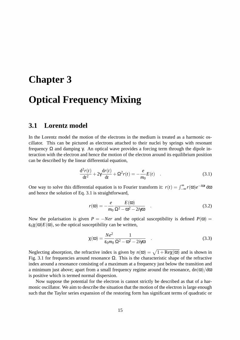
1+Reχ(ω) and is shown inFig. 3.1 for frequencies around resonanceΩ. This is the characteristic shape of the refractiveindex around a resonance consisting of a maximum at a frequency just below the transition anda minimum just above; apart from a small frequency regime around the resonance,dn(ω)/dωis positive which is termed normal dispersion.
Now suppose the potential for the electron is cannot strictly be described as that of a har-monic oscillator. We aim to describe the situation that the motion of the electron is large enoughsuch that the Taylor series expansion of the restoring form has significant terms of quadratic or
15

16 CHAPTER 3. OPTICAL FREQUENCY MIXING
-4 -2 0 2 40.6
0.7
0.8
0.9
1
1.1
1.2
1.3
Figure 3.1: The form of the dispersion of the refractive index around a resonance in the Lorentzmodel. The frequency (horizontal axis) has been scaled as(ω−ω0)/γ.
higher order. The differential equation describing the electron’s motion then has additionalanharmonic terms which we will consider tor2,
d2r(t)dt2 +2γ
dr(t)dt
+Ω2r(t)−ξr2 =− em0
E(t) . (3.4)
The differential equation is now nonlinear and is complicated to solve. However it is usual thatthe anharmonic term is small compared with the other terms and a perturbation analysis can beperformed to gain some insight. The displacement from equilibrium position is expanded asr = r0 + r1 + . . .. The differential equation taken to the lowest order (inr0) is just the harmonicLorentz equation (3.1). The next highest order gives,
d2r1(t)dt2 +2γ
dr1(t)dt
+Ω2r1(t) = ξr20(t) , (3.5)
where Eq. (3.2) is used to provide the form forr0(t).Consider the case where the optical field is monochromatic and can be describedE(t) =
[E0e−iω0t +E∗0eiω0t ]/2. The Fourier transform of this isE(ω) = [E0δ(ω−ω0)+E∗0δ(ω+ω0)]/2.The linear solutionr0 will be driven at the same frequency and hence we obtain,
r0(t) =− e2m0
[E0e−iω0t
Ω2−ω20−2iγω0
+E∗0eiω0t
Ω2−ω20−2iγω0
]. (3.6)
When this expression is squared, the terms have time dependencies ofe±2iω0t or are constant.Thus there exists driving terms forr1(t) is at frequencies±2ω0. Hence the anharmonic termhas resulted in the motion of the electron having a frequency component at twice the opticalfrequency and so will the polarisation. Similarly there will also be DC components producedfrom the constant term. What has happened here is that the anharmonic term has resulted in

3.1. LORENTZ MODEL 17
frequency mixing. Since we have only one optical frequency present the only combinations areat ω0±ω0, i.e. 2ω0 and 0.
The frequency mixing aspect can be seen more clearly if we take an optical input field that isbichromatic,E(t) = [E1e−iω1t +E2e−iω2t +cc]/2 where the cc denotes the complex conjugate.The linear solutionr0(t) will contain terms oscillating at the same frequencies,
r0(t) =− e2m0
[E1e−iω1t
Ω2−ω21−2iγω1
+E2e−iω2t
Ω2−ω22 +2iγω2
+cc
]. (3.7)
On squaring this will produce a term oscillating atω1 +ω2,
r20(t)
∣∣ω1+ω2
=e2
2m20
E1E2e−i(ω1+ω2)t[Ω2−ω2
1−2iγω1]−1[
Ω2−ω22−2iγω2
]−1. (3.8)
On inserting this into Eq. (3.5) this provides forr1(t) (e.g. by the Fourier transform methoddescribed previously),
r1(t)|ω1+ω2=
ξe2
2m0E1E2e−i(ω1+ω2)t
[Ω2− (ω1 +ω2)2−2iγ(ω1 +ω2)
]−1
×[Ω2−ω2
1−2iγω1]−1[
Ω2−ω22−2iγω2
]−1. (3.9)
Hence since the polarisation is given byP = −Ner, there is also a polarisation componentoscillating at the sum frequency,
P(ω)|ω1+ω2= −Nξe3
2m0E1E2δ(ω−ω1−ω2)
[Ω2− (ω1 +ω2)2−2iγ(ω1 +ω2)
]−1
×[Ω2−ω2
1−2iγω1]−1[
Ω2−ω22−2iγω2
]−1. (3.10)
We can extend the definition of the optical susceptibility to include these higher order effects:
P(ω)|ω1+ω2= 2ε0χ(2)(ω1,ω2)E1E2δ(ω−ω1−ω2) , (3.11)
whereχ(2) is referred to as the second-order optical susceptibility. The factor of 2 is includedsince we must allow for both orderingsE1E2 andE2E1. Eq. 3.11 is specific to the interaction oftwo monochromatic sources. It can be generalised by summing over all possible frequencies,
P(2)(ω) = ε0
∫ ∞
−∞dωa
∫ ∞
−∞dωbχ(2)(ωa,ωb)E(ωa)E(ωb)δ(ω−ωa−ωb) . (3.12)
The delta function ensures that the output polarisation oscillates at summations of the frequen-cies. Although this form looks a bit different from the linear definition of the optical susceptib-ility, we can write,
P(1)(ω) = ε0
∫ ∞
−∞dωaχ(1)(ωa)E(ωa)δ(ω−ωa) = ε0χ(1)(ω)E(ω) , (3.13)
18 CHAPTER 3. OPTICAL FREQUENCY MIXING
which shows the same form. The total contribution to the polarisation is thenP(ω) = P(1)(ω)+P(2)(ω).
By comparing Eqs. (3.10) and (3.11) we obtain,
χ(2)(ω1,ω2) = − Nξe3
4ε0m0
[Ω2− (ω1 +ω2)2−2iγ(ω1 +ω2)
]−1
×[Ω2−ω2
1−2iγω1]−1[
Ω2−ω22−2iγω2
]−1,
= −ξε20m2
0
4N2e3χ(1)(ω1 +ω2)χ(1)(ω1)χ(1)(ω2) , (3.14)
where we have substituted the linear susceptibility in the final form. This shows that if wehave a resonance in the linear susceptibility either at one of the frequency components or theirsum, there is likely to be a resonance in the second-order susceptibility. Although this result isspecific to the anharmonic Lorentz model, there is an empirical rule called Miller’s rule whichstatesχ(2)(ω1,ω2) = ∆χ(1)(ω1+ω2)χ(1)(ω1)χ(1)(ω2), where the variation of∆ with frequencyand material is much smaller than in the linear and nonlinear susceptibilities themselves.
3.2 The Nonlinear Susceptibility Tensor
In the previous section, the vectorial nature of the electric field and polarisation was ignored. Asin the case of birefringence, this can be allowed for by using tensors for the linear and nonlinearsusceptibilities. We can also expand the nonlinear polarisation beyond second-order so that
Pi(ω) = P(1)i (ω)+ P(2)
i (ω)+ P(3)i (ω)+ . . . and the nonlinear polarisation contributions can be
written,
P(1)i = ε0
∫ ∞
−∞dωaχ(1)
i j (ωa)E j(ωa)δ(ω−ωa) ,
P(2)i = ε0
∫ ∞
−∞dωa
∫ ∞
−∞dωbχ(2)
i jk (ωa,ωb)E j(ωa)Ek(ωb)δ(ω−ωa−ωb) ,
P(3)i = ε0
∫ ∞
−∞dωa
∫ ∞
−∞dωb
∫ ∞
−∞dωcχ(2)
i jkl (ωa,ωb,ωc)E j(ωa)Ek(ωb)El (ωc)
×δ(ω−ωa−ωb−ωc) .... =
... (3.15)
Summation over the repeated indicesj, k andl is implicit in the above.
3.2.1 1st order
χ(1)i j is a second rank tensor (9 elements) and is equal to the dielectric tensor less the identity
matrix (the tensor form allows birefringence to be described). The frequency of the polarisationhas to be the same as that of the electric field. Depending on the relative phase of the polarisa-tion and the electric field, the interference gives rise to optical absorption or refraction;Reχ(1)
corresponds to refraction andImχ(1) to absorption.

3.2. THE NONLINEAR SUSCEPTIBILITY TENSOR 19
3.2.2 2nd order
χ(2)i jk is a third rank tensor (27 elements). If we use a monochromatic inputE(t) = (E0e−iω0t +
E∗0eiω0t)/2 then evaluating the integrals gives for the second-order polarisation,
P(2)i (ω) = ε0
4
[χ(2)
i jk (ω0,−ω0)E0 jE∗0k +χ(2)
i jk (−ω0,ω0)E∗0 jE0k
]δ(ω−0)
+χ(2)i jk (ω0,ω0)E0 jE0kδ(ω−2ω0)
+χ(2)i jk (−ω0,−ω0)E∗0 jE
∗0kδ(ω+2ω0)
. (3.16)
As we indicated in the Lorentz anharmonic model, for a monochromatic input of frequencyω0, the second-order polarisation has frequency components at±2ω0 and 0. These give riseto second harmonic generation and optical rectification respectively. Note that there are nocomponents at the original frequencyω0. If we have a combination of frequencies present (ω1
andω2 say) we can produce the sum (ω = ω1 + ω2) and difference (ω = ω1−ω2). This evenapplies ifω2 = 0 i.e. DC and gives an alternative description of the electro-optic effect.
3.2.3 3rd order
χ(3)i jkl is a fourth rank tensor (81 elements). For a monochromatic input of frequencyω0, evalu-
ation of the integrals gives frequency components of the third-order polarisation atω = ±3ω0
(which describes third harmonic generation) and atω = ±ω0. Since we have a component atthe same frequency this will act like an absorption or refraction, only in this case the effect willbe nonlinear because of the additional electric field terms.
3.2.4 Properties of the susceptibility tensor
Intrinsic permutation symmetry In Eq. (3.15) we are at liberty to exchange pairs of indicesj, k, etc. since these are just dummy indices which are summed over the directionsx, yandz. Since the electric field component product commutates, then we must have, forexample,
χ(2)ik j (ω2,ω1) = χ(2)
i jk (ω1,ω2) . (3.17)
This property where the direction indices and frequency arguments can be permutated[e.g.( j,ω1)⇔ (k,ω2)] is called intrinsic permutation symmetry.
Reality condition The fieldE(t) and the polarsiationP(t) are physical quantities and hencemust be real. This then requires of the susceptibility, for example,
χ(2)i jk (−ω1,−ω2) = χ(2)∗
i jk (ω1,ω2) , (3.18)
that is the conjugate of the susceptibility is equivalent to negating the frequencies.

20 CHAPTER 3. OPTICAL FREQUENCY MIXING
Overall permutation symmetry If all the optical frequencies and their combinations are wellremoved from any material resonance then in addition to the intrinsic permutation sym-metry, overall permutation symmetry also applies where the combination(i,−ω1−ω2) isincluded in the sets which can be permutated leaving the nonlinear susceptibility invari-ant. So, for example,
χ(2)jik (−ω1−ω2,ω2)' χ(2)
i jk (ω1,ω2) . (3.19)
Note that unlike intrinsic permutation symmetry, overall permutation symmetry is onlyan approximation, but one which is valid in most cases of interest. Now consider thelow frequency limit such that the dispersion in the susceptibility can be ignored. In thissituation, all frequencies could be replaced by zero which implies that all frequencies areequivalent. Thus the susceptibility will be invariant if the frequency arguments alone arepermuted. Combining this with overall permutation symmetry means that the nonlinearsusceptibility is invariant under permutations of the direction indices. This gives, forexample,
χ(2)ik j (ω1,ω2)' χ(2)
i jk (ω1,ω2) . (3.20)
This property is called Kleinmann symmetry. Once again it is important to note that thisis just an approximation that applies in the low frequency limit, far from any materialresonances.
Causality So far we have been using the frequency domain for describing the optical polar-isation. The linear susceptibility was definedP(ω) = ε0χ(ω)E(ω) which is a product.Now under Fourier transforming, a product becomes a convolution so we have in the timedomain,
P(t) =ε0
2π
∫ ∞
−∞χ(τ)E(t− τ)dτ . (3.21)
Now the principle of causality states that any feature in the input (electric field in thiscase) cannot affect the output (polarisation) at earlier times. That is effect cannot precedecause. Hence in the above convolutionE(t−τ) cannot influenceP(t) if t < t−τ i.e.τ < 0.This then requiresχ(τ) = 0 for τ < 0. One way of expressing this is to setχ(τ) = χ(τ)θ(τ)whereθ(τ) is the Heaviside (step) function. If we Fourier transform this expression, theproduct becomes a convolution and we obtain the relationship,
χ(ω) =1iπ
P∫ ∞
−∞
χ(Ω)dΩΩ−ω
, (3.22)
whereP is used to denote a principal parts integral. Because of the extra factori inthis relation, by separating this equation into real and imaginary parts, one can relate thereal part ofχ solely in terms of its imaginary part and vice versa. Hence if onlyImχ issupplied (across the entire spectral range),Reχ can be generated. This is one exampleof a dispersion relation of which the best known is the Kramers-Kronig relation relatingrefractive index to absorption coefficient. For a wider discussion on dispersion relationsand their applicability to the nonlinear case see [5].
Chapter 4
Second-Order Optical Nonlinearities
4.1 Contracted tensor for 2nd-order nonlinearities
In determining the second-order polarisationP(2)(ω), summation takes place over all per-mutations, e.g. in the case of second harmonic generation, if the electric field has compon-ents along they and z axes, there will be a polarisation generated parallel to thex axis:
χ(2)xyzEyEz+ χ(2)
xzyEzEy. Since the same combination of fields occurs in both terms then we cancontract these to a single term. If we useP(2)(ω) = [P2ω0δ(ω−2ω0)+ P−2ω0δ(ω + 2ω0)]/2andE(ω) = [Eω0δ(ω−ω0)+E−ω0δ(ω + ω0)]/2 then we can re-write the second-order polar-isation as,
P2ω0x
P2ω0y
P2ω0z
= ε0
d11 d12 d13 d14 d15 d16
d21 d22 d23 d24 d25 d26
d31 d32 d33 d34 d35 d36
(Eω0x )2
(Eω0y )2
(Eω0z )2
2Eω0y Eω0
z
2Eω0x Eω0
z
2Eω0x Eω0
y
, (4.1)
where the second subscript on the coefficientd relates to the conventional axes by, 1:xx, 2:yy,3:zz, 4:yzor zy, 5:zxor xzand 6:xy or yx. It can be seen that the contractedd-tensor for SHGis simply related to the conventional susceptibility tensor bydi jk(ω,ω) = χ(2)
i jk (ω,ω)/2. Notethat we have used intrinsic permutation symmetry to reduce the 27 elements to 18 independentones.
If Kleinmann symmetry can be applied then the contracted tensor notation can be extendedto nondegenerate interactions (ω1 6= ω2),
Pω1+ω2x
Pω1+ω2y
Pω1+ω2z
= 2ε0
d11 d12 d13 d14 d15 d16
d21 d22 d23 d24 d25 d26
d31 d32 d33 d34 d35 d36
Eω1x Eω2
x
Eω1y Eω2
y
Eω1z Eω2
z
Eω1y Eω2
z +Eω2y Eω1
z
Eω1z Eω2
x +Eω2z Eω1
x
Eω1x Eω2
y +Eω2x Eω1
y
, (4.2)
21

22 CHAPTER 4. SECOND-ORDER OPTICAL NONLINEARITIES
Triclinic 1
d11 d12 d13 d14 d15 d16d21 d22 d23 d24 d25 d26d31 d32 d33 d34 d35 d36
Monoclinic 2
0 0 0 d14 0 d16d21 d22 d23 0 d25 00 0 0 d34 0 d36
m
d11 d12 d13 0 d15 00 0 0 d24 0 d26
d31 d32 d33 0 d35 0
Orthorhombic 222
0 0 0 d14 0 00 0 0 0 d25 00 0 0 0 0 d36
mm2
0 0 0 0 d15 00 0 0 d24 0 0
d31 d32 d33 0 0 0
Tetragonal 4
0 0 0 d14 d15 00 0 0 d15 d14 0
d31 d31 d33 0 0 0
4
0 0 0 d14 d15 00 0 0 d15 d14 0
d31 d31 0 0 0 d36
422
0 0 0 d14 0 00 0 0 0 d14 00 0 0 0 0 0
4mm
0 0 0 0 d15 00 0 0 d15 0 0
d31 d31 d33 0 0 0
42m
0 0 0 d14 0 00 0 0 0 d14 00 0 0 0 0 d36
Cubic 432
0 0 0 0 0 00 0 0 0 0 00 0 0 0 0 0
43m
23
0 0 0 d14 0 00 0 0 0 d14 00 0 0 0 0 d14
Trigonal 3
d11 d11 0 d14 d15 d22
d22 d22 0 d15 d14 d11d31 d31 d33 0 0 0
32
d11 d11 0 d14 0 00 0 0 0 d14 d110 0 0 0 0 0
3m
0 0 0 0 d15 d22
d22 d22 0 d15 0 0d31 d31 d33 0 0 0
Hexagonal 6
0 0 0 d14 d15 00 0 0 d15 d14 0
d31 d31 d33 0 0 0
6
d11 d11 0 0 0 d22
d22 d22 0 0 0 d110 0 0 0 0 0
622
0 0 0 d14 0 00 0 0 0 d14 00 0 0 0 0 0
6mm
0 0 0 0 d15 00 0 0 d15 0 0
d31 d31 d33 0 0 0
6m2
0 0 0 0 0 d22
d22 d22 0 0 0 00 0 0 0 0 0
Table 4.1: The form of thed-tensor for the crystal symmetry classes which do not possessinversion symmetry. A bar over an entry indicates the negative.
wheredi jk(ω1,ω2) = χ(2)i jk (ω1,ω2)/2 = χ(2)
i jk (ω2,ω1)/2.
As in the case of the electro-optic coefficient, the number of independent elements can befurther reduced with symmetry considerations. First of all if the material exhibits inversionsymmetry then all thed tensor elements are zero. If we start fromP2ω
i = ε0di jkEωj Eω
k andthen apply the inversion operator, for materials with inversion symmetrydi jk is unaltered and,−P2ω
i = ε0di jk(−Eωj )(−Eω
k ). This is only consistent ifdi jk =−di jk and hencedi jk = 0. Grouptheory can be applied to investigate other symmetry properties. Table 4.1 shows the form of thed-tensor for the 18 crystal classes that do not exhibit inversion symmetry.
If Kleinmann symmetry can be applied (low frequency, well removed from resonances) the
4.2. EM PROPAGATION WITH A SECOND-ORDER NONLINEARITY 23
18 tensor elements are further reduced to 10. The relevant equalities are summarised in Table4.2. As an example consider KTP (KTiOPO4) which has orthorhombic symmetry of classmm2and hence by Table 4.1 has 5 independent, non-zero components. At a wavelength of 880 nm,these have been measured as [6]:d15 = 2.04 pmV−1, d31 = 2.76 pmV−1, d24 = 3.92 pmV−1,d32 = 4.74pmV−1 andd33 = 18.5 pmV−1. Kleinmann symmetry specifiesd15' d31 andd24'd32 which is only approximately true (within around 30%) in this case. Note that in this examplethe on-diagonal elementd33≡ dzzz is several times larger than the off-diagonal elements. Thisbehaviour is quite common among materials which exhibit a second order nonlinearity.
di jk di j
dxyy = dyxy d12 = d26
dxzz= dzxz d13 = d35
dxyz= dyzx= dzxy d14 = d25 = d36
dxzx= dzxx d15 = d31
dxxy = dyxx d16 = d21
dyzz= dzyz d23 = d34
dyyz= dzyy d24 = d32
Table 4.2: Equalities among thed-tensor elements under application of Kleinmann symmetry.
Rather than completely write out Eqs. (4.1) and (4.2) every time, we will denote this by theshorthand tensor multiplication,
Pω1+ω2 = 2ε0d(ω1,ω2) : Eω1Eω2 . (4.3)
Furthermore, it is quite common to split the fields into magnitude and direction, i.e.Eω1 = e1Eω1
etc. wheree1 is a unit vector. A scaler quantitydeff is commonly used which hides the detailsof the tensor multiplication:deff = ep · [d(ω1,ω2) : e1e2]. This allows the vector equation (4.3)to be written in scaler form.
4.2 EM Propagation with a Second-Order Nonlinearity
4.2.1 Slowly Varying Envelope Approximation
Start from the Maxwell curl equations∇×E(t) =−∂B(t)/∂t and∇×H(t) = j(t)+∂D(t)/∂t,assume a non-magnetic materialB = µ0H and takej = σE. We will split the polarisation intolinear and nonlinear components,D = ε0E+P = ε0εrE+PNL . Combining the two curl equa-tions then gives the second order PDE,
∇×∇×E(t) =−µ0σ∂E(t)
∂t− εr
c2
∂2E(t)∂t2 −µ0
∂2PNL(t)∂t2 . (4.4)
Now the properties of the vector differential operators gives that∇×∇×E = ∇(∇ ·E)−∇2Eand if there are no free charges, we also have∇ ·E = 0. The time derivatives can also be

24 CHAPTER 4. SECOND-ORDER OPTICAL NONLINEARITIES
simplified by Fourier transforming to the frequency domain to give,
∇2E(ω) =(−iωµ0σ− ω2εr
c2
)E(ω)−µ0ω2PNL(ω) . (4.5)
Now let us insert a plane wave propagating in one direction only, which we will take to beforward (taken as parallel to thez-axis here). We will allow the amplitude of this wave to varyon propagation and takeE(ω) = E(ω,z)eikz where the value of the wavevectork =
√εrω/c is
obtained from solution of the wave equation [Eq. 4.5 without the nonlinear polarisation term].On taking the space differential,
∇2E(ω)→ d2E(ω)dz2 =
[d2E(ω,z)
dz2 +2ikdE(ω,z)
dz−k2E(ω,z)
]eikz . (4.6)
Note that the final term proportional toE will exactly cancel a term in Eq. 4.5. Now let usassume that the nonlinear term is small (which is the case except in extreme circumstanceswhich will not be dealt with here) and hence the modification from the linear case will be small.This tells us that the envelope will depart only slightly from its linear (constant) value. It willcertainly vary much more slowly than the oscillation of the underlying wave — hence thisapproximation is conventionally termed the slowly varying envelope (or amplitude) approxim-ation. This allows us to use|d2E/dz2| ¿ |kdE/dz| and neglect the second-order derivative inthe envelope. Hence we reduce the second order differential equation to the first order one,
dE(ω,z)dz
=−α2
E(ω,z)+iω2µ0
2kPNL(ω)e−ikz , (4.7)
where we have substituted the absorption coefficientα = ωµ0σ/k. Although this is termed theslowly varying envelope approximation, the key approximation is the unidirectional nature ofthe wave propagation. If propagation both in the forward and backward directions occurs, thencoupled terms arise which prevent this simplification. On the right-hand side of Eq. 4.7 the firstterm describes linear loss and the second term describes a nonlinear polarisation source for thewave.
Eq. (4.7) is relevant for any order of nonlinearity. In this chapter we are concentrating onsecond order nonlinearities for frequency mixing. Let us consider the interaction between twowaves of frequencyω1 andω2, producing a polarisation at the sum frequencyω3 = ω1 + ω2.Using the contractedd-tensor notation we have,Pω3 = 2ε0d(ω1,ω2) : Eω1Eω2. Inserting thisinto Eq. (4.7) gives,
dEω3
dz= −α3
2Eω3 +
iω23
2k3c2d(ω1,ω2) : Eω1Eω2ei∆kz ,
dEω1
dz= −α1
2Eω1 +
iω21
2k1c2d(ω3,−ω1) : Eω3E−ω2e−i∆kz ,
dEω2
dz= −α2
2Eω2 +
iω22
2k2c2d(ω3,−ω1) : Eω3E−ω1e−i∆kz , (4.8)

4.2. EM PROPAGATION WITH A SECOND-ORDER NONLINEARITY 25
where we have used∆k = k1 + k2− k3 andk3 = k(ω3) etc. Also of relevance the interactionswhere the difference betweenω3 andω1 producesω2 and the difference betweenω3 andω2
producesω1 which are also listed. Note thatE−ω1 = (Eω1)∗.
4.2.2 Manley-Rowe Relations
Now consider the case that we are considering frequencies well removed from any materialresonances. This is equivalent to stating we are concerned with a frequency region that istransparent and henceα1, α2, α3 = 0. We can also apply overall permutation symmetry whichstatesd(ω3,−ω2) = d(ω3,−ω1) = d(ω1,ω2). For simplicity we use the substitutiondeff =d(ω1,ω2) : e1e2. Hence Eqs. (4.8) can be rewritten as,
dEω3
dz=
iω23
2k3c2deffEω1Eω2ei∆kz ,
dEω1
dz=
iω21
2k1c2deffEω3(Eω2)∗e−i∆kz ,
dEω2
dz=
iω22
2k2c2deffEω3(Eω1)∗e−i∆kz . (4.9)
In SI units the irradiance is defined in terms of the electric field amplitude as,Iω =ε0cn(ω)|Eω|2/2, wheren(ω) is the refractive index. Differentiating this gives,
dIω
dz=
ε0cn0(ω)2
[(Eω)∗
dEω
dz+Eω
(dEω
dz
)∗]. (4.10)
Inserting the electric field derivatives and usingk = nω/c then gives,
dIω3
dz=
ε0ω3
2
[ideffE
ω1Eω2(Eω3
)∗ei∆kz− ideff
(Eω1Eω2
)∗Eω3e−i∆kz
],
dIω1
dz=
ε0ω1
2
[ideff
(Eω1Eω2
)∗Eω3e−i∆kz− ideffE
ω1Eω2(Eω3
)∗ei∆kz
],
dIω2
dz=
ε0ω2
2
[ideff
(Eω1Eω2
)∗Eω3e−i∆kz− ideffE
ω1Eω2(Eω3
)∗ei∆kz
]. (4.11)
We can see from the above that,
1ω3
dIω3
dz=− 1
ω1
dIω1
dz=− 1
ω2
dIω2
dz. (4.12)
Now irradiance is defined as optical energy flowing through a unit area per unit time. Thephoton energy ishω and hence the ratio of the irradiance to the optical frequency is proportionalto the number of photons passing through a unit area per unit time or in other words the photonflux. Hence Eq. (4.12) can be restated as the change in the number of photons atω3 is thenegative of the change in the number of photons atω1 or ω2 (which are equal):∆N3 =−∆N1 =−∆N2. These are known as the Manley-Rowe relations. These seem intuitively correct fromsimple energy conservation; we are far from material resonances so the only energy flow can bebetween the waves of different frequency.

26 CHAPTER 4. SECOND-ORDER OPTICAL NONLINEARITIES
4.2.3 Sum frequency generation:ω1+ω2→ ω3
Let us assume that there is initially no light of the sum frequencyω3 present. Let us also initiallyexamine the case of low conversion efficiency such that any depletion of the frequenciesω1
andω2 can be neglected, i.e.dEω1/dz, dEω2/dz≈ 0. This simplification allows just one of thedifferential equations to be studied instead of the complete set. Let us also assume that the linearloss can be neglected,α3 = 0 and hence we have for the evolution of the light at frequencyω3,
dEω3
dz=
iω3
cn3deffE
ω1Eω2ei∆kz , (4.13)
where we have used as shorthand for the refractive indexn3 = n(ω3). SinceEω1 andEω2 aretreated as constant (low conversion efficiency), this can be easily integrated along the length ofthe crystal to give,
Eω3(L) =ω3deff
cn3Eω1Eω2
(ei∆kL−1)∆k
=ω3deffL
cn3Eω1Eω2ei∆kL/2sinc
∆kL2
, (4.14)
where sincx = (sinx)/x. Now writing this instead in terms of the irradiance,Iω =ε0cn(ω)|Eω|2/2,
Iω3(L) =2ω2
3
ε0c3
d2eff
n1n2n3L2Iω1Iω2sinc2 ∆kL
2. (4.15)
There are several points to make about the generation of the sum frequency described by Eq.(4.15): the irradiance of the generated light is (1) proportional to a material factord2
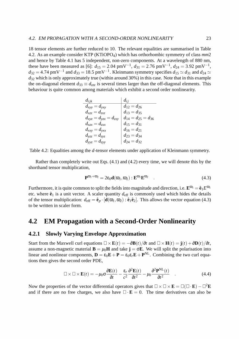
eff/n3 (wewill see this is the usual factor in second order processes) (2) proportional to both the irradi-ance atω1 and atω2 (3) grows quadratically with distance (L2) and (4) depends on the factorsinc2∆kL/2. This last factor is shown plotted in Fig. 4.1. It can be seen that this has a max-imum value of 1 at∆kL/2 = 0 but falls off rapidly away from this. Hence it is important forefficient generation to operate at∆k = 0 i.e. k1 + k2 = k3. This is termed phasematching sincewe are matching the phase velocity of the existing wave (k3) to that of the nonlinear polarisa-tion (k1 +k2). Phase-matching can be thought of as photon momentum conservation (since thephoton’s momentum is given byhk) just as the Manley-Rowe relations describe photon energyconservation.
4.2.4 Second harmonic generation:ω+ω→ 2ωSecond harmonic generation is just a special case of sum frequency generation where an opticalwave interacts with itself to generate the sum frequency. Instead of three coupled differentialequations to consider, in this case we require just two. Let us assume that we are removed fromresonances so that linear loss can be neglected and overall permutation symmetry applied. Inthe low conversion efficiency approximation we get a result similar to the previous case with a
4.2. EM PROPAGATION WITH A SECOND-ORDER NONLINEARITY 27
−4π −2π 0 2π 4π
0.2
0.4
0.6
0.8
1.0
Figure 4.1: Plot ofsinc2x, indicating the sensitivity of phase-matching.
sinc2∆kL/2 phase=matching dependence. Here we shall include the effects of pump depletionso we require both differential equations,
dE2ω
dz=
iωcn2ω
deff(ω,ω)(Eω)2
ei∆kz ,
dEω
dz=
iωcnω
deff(ω,ω)E2ω (Eω)∗
e−i∆kz , (4.16)
where∆k = 2kω− k2ω. We can combine these two by differentiating the second equation andsubstituting fordE2ω/dz from the first to give,
d2Eω
dz2 + i∆kdEω
dz+
ω2d2eff
c2n2ωn2ω
[nω
∣∣Eω∣∣2−n2ω∣∣E2ω∣∣2
]Eω = 0 . (4.17)
Now if we initially have no second harmonic,E2ω(z= 0) = 0, then we can use Manley-Roweto getI2ω(z) = Iω(z= 0)− Iω(z). In terms of electric fields this gives,n2ω|E2ω|2 = nω(|Eω(z=0)|2−|Eω|2). Substituting gives a differential equation inEω alone,
d2Eω
dz2 + i∆kdEω
dz+
ω2d2eff
c2nωn2ω
[2∣∣Eω∣∣2−
∣∣E2ω(z= 0)∣∣2
]Eω = 0 . (4.18)
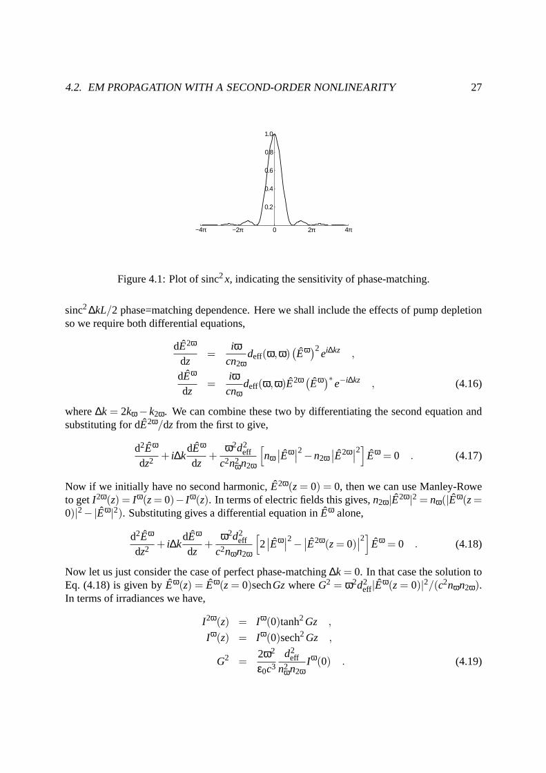
Now let us just consider the case of perfect phase-matching∆k = 0. In that case the solution toEq. (4.18) is given byEω(z) = Eω(z= 0)sechGzwhereG2 = ω2d2
eff|Eω(z= 0)|2/(c2nωn2ω).In terms of irradiances we have,
I2ω(z) = Iω(0)tanh2Gz ,
Iω(z) = Iω(0)sech2Gz ,
G2 =2ω2
ε0c3
d2eff
n2ωn2ω
Iω(0) . (4.19)
28 CHAPTER 4. SECOND-ORDER OPTICAL NONLINEARITIES
Note once again the material factord2eff/n3 appears. The functional forms of these are shown in
Fig. 4.2. Note that for small distances the growth of SHG is proportional toz2 as we discoveredpreviously. However, it can be seen that this saturates when the power in the second harmonicbecomes an appreciable fraction of that in the fundamental.
0.5 1 1.5 2 2.5 3
0.2
0.4
0.6
0.8
1
Figure 4.2: Plot of the growth of second harmonic and pump depletion with distance (normal-ised to1/G).
4.2.5 Parametric upconversion:ω1+ω2→ ω3
This is yet another extension of sum frequency generation. In this case we will consider inputsat frequenciesω1 andω2 generating the sum frequency atω3 for which initially is not present.The beam atω2 is assumed to be the more intense and hence its depletion can be ignored,dEω2/dz≈ 0. However, we will include the depletion of the beam atω1. It is conventionalto call the intense (ω2) beam the pump and the less intense beam (ω1) the signal. In fact thedescription upconversion arises because we will be raising the frequency of the signal fromω1
to ω3. As we can ignore the evolution of the pump we need only consider the pair of coupleddifferential equations (making the usual assumption of remote from material resonances),
dEω3(z)dz
=iω3
2cn3deffE
ω1(z)Eω2ei∆kz ,
dEω1(z)dz
=iω1
2cn1deffE
ω3(z)(Eω2
)∗e−i∆kz . (4.20)
For perfect phase-matching,∆k= 0, Eqs. (4.20) can be combined to eliminateEω3 which resultsin the undamped harmonic oscillator differential equation. The solution isEω1(z) = Eω1(z=0)cosGzwhereG2 = ω1ω3d2
eff|Eω2|2/(4c2n1n3). In terms of irradiances we have,
Iω1(z) = Iω1(0)cos2Gz ,
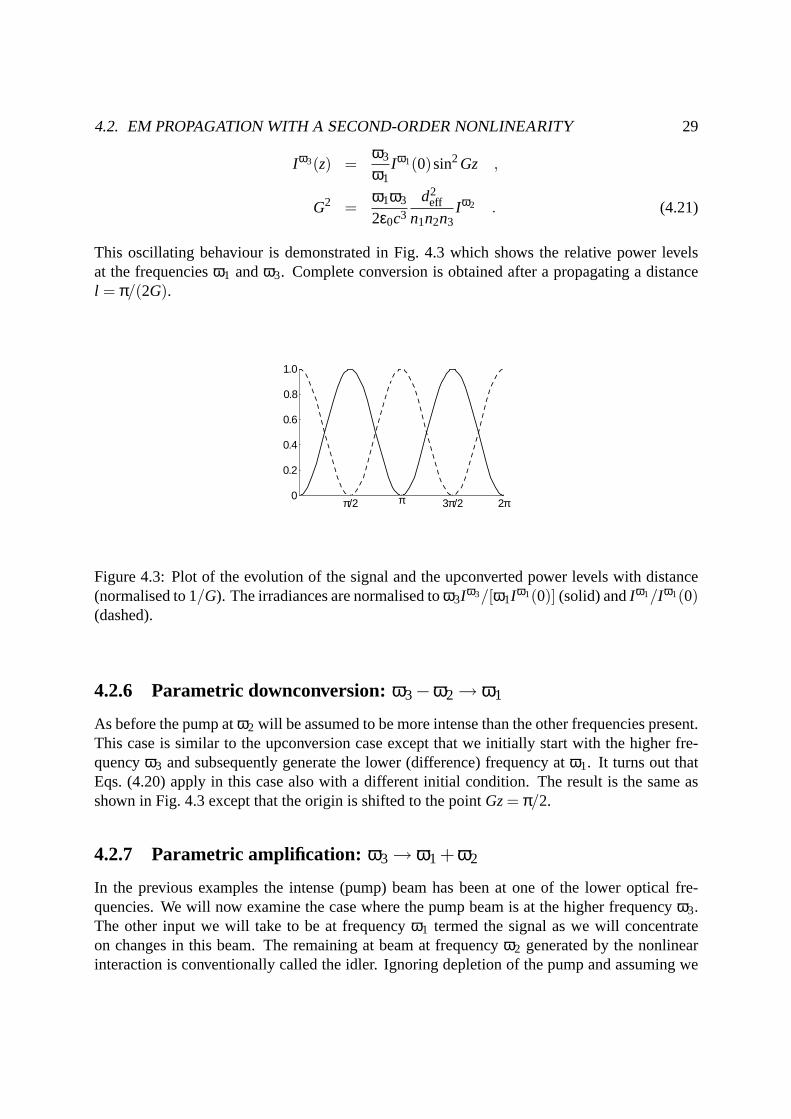
4.2. EM PROPAGATION WITH A SECOND-ORDER NONLINEARITY 29
Iω3(z) =ω3
ω1Iω1(0)sin2Gz ,
G2 =ω1ω3
2ε0c3
d2eff
n1n2n3Iω2 . (4.21)
This oscillating behaviour is demonstrated in Fig. 4.3 which shows the relative power levelsat the frequenciesω1 andω3. Complete conversion is obtained after a propagating a distancel = π/(2G).
π/2 π 3π/2 2π0
0.2
0.4
0.6
0.8
1.0
Figure 4.3: Plot of the evolution of the signal and the upconverted power levels with distance(normalised to1/G). The irradiances are normalised toω3Iω3/[ω1Iω1(0)] (solid) andIω1/Iω1(0)(dashed).
4.2.6 Parametric downconversion:ω3−ω2→ ω1
As before the pump atω2 will be assumed to be more intense than the other frequencies present.This case is similar to the upconversion case except that we initially start with the higher fre-quencyω3 and subsequently generate the lower (difference) frequency atω1. It turns out thatEqs. (4.20) apply in this case also with a different initial condition. The result is the same asshown in Fig. 4.3 except that the origin is shifted to the pointGz= π/2.
4.2.7 Parametric amplification: ω3→ ω1+ω2
In the previous examples the intense (pump) beam has been at one of the lower optical fre-quencies. We will now examine the case where the pump beam is at the higher frequencyω3.The other input we will take to be at frequencyω1 termed the signal as we will concentrateon changes in this beam. The remaining at beam at frequencyω2 generated by the nonlinearinteraction is conventionally called the idler. Ignoring depletion of the pump and assuming we

30 CHAPTER 4. SECOND-ORDER OPTICAL NONLINEARITIES
are remote from resonances, we have to consider the following pair of differential equations,
dEω1(z)dz
=iω1
2cn1deffE
ω3(Eω2(z)
)∗e−i∆kz ,
dEω2(z)dz
=iω2
2cn2deffE
ω3(Eω1(z)
)∗e−i∆kz . (4.22)
Taking perfect phase-matching (∆k= 0), and combining Eqs. (4.22) to eliminate one of the elec-tric fields results in the undamped harmonic oscillator equation with a sign change. Assumingthat there is initially no light of frequencyω2 we obtain the solutionEω1(z)= Eω1(z= 0)coshGzwhereG2 = ω1ω2d2
eff|Eω3|2/(4c2n1n2). In terms of irradiances we have,
Iω1(z) = Iω1(0)cosh2Gz ,
Iω2(z) =ω2
ω1Iω1(0)sinh2Gz ,
G2 =ω1ω2
2ε0c3
d2eff
n1n2n3Iω3 . (4.23)
For large amplifications,GzÀ 1, both signal and idler will be dominated by the factore2Gz, i.e.it will appear we have a gain coefficient2G which is proportional to the square root of the pumpirradiance.
One application of the optical parametric amplifier is to directly amplify an imput signal.Alternatively, it can be used in a similar fashion to a laser in that the amplifier is placed in a cav-ity and the oscillating optical power is initially amplified from noise (e.g. quantum fluctuationsor black-body). This device is called an optical parametric oscillator (OPO). Like a laser, oscil-lation will preferentially occur at the maximum gain which automatically specifies operation atperfect phase-matchingk1+k2 = k3. If there is some means of controlling the phase-matching,then this provides a means of tuning the OPO. Again like a laser, for oscillation to occur opticalgain must exceed optical losses (transmission at mirrors, absorption, scattering, etc.) and thefeedback is positive. For a laser, this gives rise to a threshold in whatever pumping mechanism isused. For an OPO the same form of threshold exists in that the gain coefficient2G must exceedsome critical value. SinceG ∝
√Iω3, this provides a threshold in the optical pump power.
There are several different forms of OPO. In the simplest, singly resonant form, a cavityis formed for only one of the generated frequencies,ω1 (say). The doubly resonant form hascavities for both generated frequencies,ω1 andω2. The doubly resonant OPO has the lowerthreshold but is more complex to set up (since we have to satisfy that both these frequenciesare cavity modes and satisfyω1 +ω2 = ω3) and as a consequence is less stable. A triply reson-ant OPO has also been sometimes used where an additional cavity for the pump increases thecirculating optical power in the nonlinear element compared to the input power level.
A summary of the six configurations discussed is shown in Fig. 4.4.
4.2.8 Phase shift in fundamental (cascaded nonlinearity)
The principle of causality states that output cannot precede an input. One of the consequencesof this is if some frequency component is attenuated then the remaining frequency components

4.2. EM PROPAGATION WITH A SECOND-ORDER NONLINEARITY 31
ω
ωω
1
2
3
ω
2ω
ω
ωω
1
2
3
ω
ωω
ω
ωω
ω
ωω
2
3
1
3
1
2
3
1
2
(a) (b) (c)
(d) (e) (f)
Figure 4.4: Summary of the six optical frequency conversion configurations discussed in thissection takingω1+ω2 = ω3: (a) sum frequency generation, (b) second harmonic generation, (c)parametric upconversion, (d) parametric downconversion, (e) parametric amplification and (e)optical parametric oscillation. In each case the larger arrow indicates the more intense pump.
must have a phase shift to maintain causality. Mathematically this is known as a dispersionrelation of which the most well known example is the Kramers-Kronig relation relating therefractive index to the absorption coefficient spectrum. Now in the case of frequency conversion,the power is being attenuated in at least one of the input beams. Now of course the poweris being transferred to another frequency instead of a material excitation, but causality stillapplies and there will be an associated phase shift. The mechanism by which this occurs isthat away from perfect phase-matching, conversion to the new frequency will be followed byback-conversion when the nonlinear polarisation source and the electric field drift out of phase.This interference can produce a wave with a different phase to the original. Of course sincethe frequency conversion is a nonlinear process and depends on irradiance, the associated phaseshift will also be irradiance dependent.
The nonlinear phase shift will be present in all the configurations studied but we use secondharmonic generation as an example. If we assume a low conversion efficiency,|Eω(z)| ≈|Eω(z= 0)|, Eq. (4.18) becomes a linear homogeneous differential equation,
d2Eω
dz2 + i∆kdEω
dz+G2Eω = 0 . (4.24)
Now let us take the approximation|∆k| À G which is usually the case for low conversionefficiency. Then the second-order derivative can be neglected and the solution of the differen-tial can be approximated asEω(z) = Eω(z = 0)eiG2z/∆k. This shows we obtain a phase shift∆φ = G2z/∆k which is proportional to the irradiance and distance propagated. Note that it isinversely proportional to∆k and hence can be made large for small phase mis-match (althoughthe approximation in dering this breaks down close to perfect phase matching) and that the signof the phase shift is the same as the phase mis-match which can, in principle, be changed. Ifwe identify an effective nonlinear refractive coefficientneff
2 such that∆φ = 2πneff2 Iz/λ then we

32 CHAPTER 4. SECOND-ORDER OPTICAL NONLINEARITIES
obtain,
neff2 =
4πε0c
1∆kλ
d2eff
n2ωn2ω
. (4.25)
For small phase mis-matches we cannot simplify Eq. (4.18) in this fashion. Analytic solu-tions are possible using Jacobi elliptic functions [7] but in many cases numerical solutions aremore convenient. For example in Fig. 4.5 we show the fundamental phase shift and throughputas a function of distance for three different values of initial fundamental irradiance (this wascalculated using the built-in numerical differential equation solver inMathematica). Note thatfor the small phase mis-matches the phase shift is not simply linearly dependent on distance asindicated by the low conversion efficiency approximation. We can also plot the phase shift andthroughput as a function of fundamental irradiance and this is shown in Fig. 4.6.
π/2 π 3π/2 2π
Phase Shift
0
π/4
π/2
3π/4
π/2 π 3π/2 2π
Throughput
0
0.2
0.4
0.6
0.8
1.0
Figure 4.5: Fundamental phase shift and throughput as a function of distance (scaled to1/∆k).The input irradiances have been scaled but are in the ratio 10(solid):5(dash):2(long dash).
4.2.9 Electro-optic effect revisited
The contractedd-tensor notation can also be used to describe the electro-optic effect. If wetake one of the fields as DC, e.g.ω2, k2 → 0, then a “nonlinear” polarisation is obtained at thesame frequency as the optical input. Phase-matching will be automatic and the slowly varyingenvelope approximation gives,
dEω
dz=
iωcnω
deff(0,ω)EDCEω . (4.26)
The solution of this isEω(z) = Eω(z= 0)eiωdeffEDCz/(nc), i.e. the optical beam develops a phaseshift ∆φ = ωdeffEDCz/(nc).
Now from the electro-optic effect we had∆(1/n2) = rEDC and hence for small changes inrefractive index produces a phase change∆φ =−ωn3rEDCz/(2c). Comparing these two forms

4.3. PHASE MATCHING 33
0 4 8 12 16Optical Power (scaled)
0
1
2
3
Non
linea
r P
hase
Shi
ft
0.0
0.2
0.4
0.6
0.8
1.0
Fun
dam
enta
l Thr
ough
put
∆kL=π
0 1 2 3 4Optical Power (scaled)
0
1
2
3
Non
linea
r P
hase
Shi
ft
0.0
0.2
0.4
0.6
0.8
1.0
Fun
dam
enta
l Thr
ough
put
∆kL=2π
Figure 4.6: Fundamental phase shift and throughput as a function of scaled irradiance for twofixed values of∆kL.
gives us that the electro-optic coefficient is simply proportional to thedeff(0,ω) coefficient,r =−2deff/n4. Note that since the refractive index is dimensionless, the electro-optic coefficientand thed coefficient are in the same units usually given in pmV−1. If we take more care toinclude the tensor nature of these coefficients we would find that in the contracted notation it isthe transposes that are related,r i j =−2d ji/n4. In fact we can see that by comparing Tables 4.1and 2.1 that the symmetry properties of the tensors reflect this transpose relation.
4.3 Phase matching
For second-order processes we have to satisfyω1+ω2 = ω3 (energy conservation). For efficientconversion phase-matching is also required,k1 + k2 = k3 (momentum conservation). Sincek = ωn/c, phase-matching is satisfied ifn1 = n2 = n3. The problem is that materials are usuallydispersive and the refractive index varies with frequency. Normal dispersion has the refractiveindices increasing with frequency,n3 > n1, n2. This obviously makes it difficult to achievephase-matching.
4.3.1 Birefringent phase-matching
The most common technique to obtain phase-matching is to use birefringence to compensatefor dispersion. The idea is that at each frequency there is a pair of refractive indices (orthogonalpolarisations) and the difference between these is adjusted to compensate for dispersion. The ex-traordinary refractive index in a uniaxial crystal as a function of angle between the propagation

34 CHAPTER 4. SECOND-ORDER OPTICAL NONLINEARITIES
direction and the optic axis is given by,ne(θ) = (sin2θ/n2e + cos2θ/n2
o)−1/2. Fig. 4.7 demon-
strates how phase-matching could be achieved for second harmonic generation for a particularpropagation direction by selecting the propagation direction such thatnω
o (θm) = n2ωe (θm)
z
xmθ
on2ω
noω
ne2ω
neω
k
Figure 4.7: Birefringent phase-matching for second harmonic generation in a negative uniaxialcrystal. For propagation at a particular angleθm to the optic axis,nω
o = n2ωe .
For a three wave interaction a possible configuration is shown in Fig. 4.8 for a negativeuniaxial crystal. Here there are a couple of possible phase-matching scenarios outlined in Table4.3: in type I phase-matching the low frequency components have parallel polarisations, in typeII the low frequency components are orthogonal.
x
z
k k k k k ko1
e1
o2
e2
o3
e3
Figure 4.8: Birefringent phase-matching for three wave interaction in a negative uniaxial crystal.For propagation at a particular angleθm to the optic axis,ko
1 +ko2 = ke
3.
If we expand the phase mis-match around the angleθm which corresponds to perfect phase-matching we have∆k ∝ ∆θ+O(∆θ2) where∆θ = θ−θm. Since thesinc2 efficiency dependenceof phase mis-match is very tight, this means that the propagation direction must, in general, be
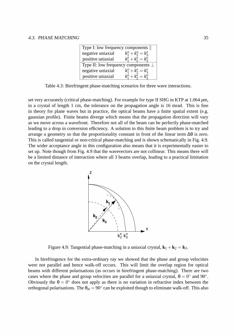
4.3. PHASE MATCHING 35
Type I: low frequency components‖negative uniaxial ko
1 +ko2 = ke
3positive uniaxial ke
1 +ke2 = ko
3Type II: low frequency components⊥negative uniaxial ko
1 +ke2 = ke
3positive uniaxial ko
1 +ke2 = ko
3
Table 4.3: Birefringent phase-matching scenarios for three wave interactions.
set very accurately (critical phase-matching). For example for type II SHG in KTP at 1.064µm,in a crystal of length 1 cm, the tolerance on the propagation angle is 16 mrad. This is finein theory for plane waves but in practice, the optical beams have a finite spatial extent (e.g.gaussian profile). Finite beams diverge which means that the propagation direction will varyas we move across a wavefront. Therefore not all of the beam can be perfectly phase-matchedleading to a drop in conversion efficiency. A solution to this finite beam problem is to try andarrange a geometry so that the proportionality constant in front of the linear term∆θ is zero.This is called tangential or non-critical phase-matching and is shown schematically in Fig. 4.9.The wider acceptance angle in this configuration also means that it is experimentally easier toset up. Note though from Fig. 4.9 that the wavevectors are not collinear. This means there willbe a limited distance of interaction where all 3 beams overlap, leading to a practical limitationon the crystal length.
x
z
k ke2
o3
kk
k1
23
Figure 4.9: Tangential phase-matching in a uniaxial crystal,k1 +k2 = k3.
In birefringence for the extra-ordinary ray we showed that the phase and group velocitieswere not parallel and hence walk-off occurs. This will limit the overlap region for opticalbeams with different polarisations (as occurs in birefringent phase-matching). There are twocases where the phase and group velocities are parallel for a uniaxial crystal,θ = 0 and90.Obviously theθ = 0 does not apply as there is no variation in refractive index between theorthogonal polarisations. Theθm = 90 can be exploited though to eliminate walk-off. This also

36 CHAPTER 4. SECOND-ORDER OPTICAL NONLINEARITIES
has the advantage of automatically being tangential phase-matching with parallel wavevectorsthus also eliminating the other overlap problem discussed in the previous paragraph.
Hence the ideal situation for birefringent phase-matching is (non-critical) tangential atθm =90. Sometimes it is necessary to temperature tune the crystal to achieve this, but the advantagesof this geometry outweighes the disadvantage of the necessity of a uniform temperature stage.To date the most attractive materials for second-order processes are LiB3O5 and β-BaB2O4
because of the possibility of non-critical phase-matching and relatively low damage thresholds.For a wider list of current second-order nonlinear materials consult [8] and references therein.
4.3.2 Quasi-phase-matching
Birefringent phase-matching can be seen to have some problems yet it is the most commonlyused technique. The largest nonlinear coefficients occur though for either non-birefringentmaterials (e.g. for GaAs in the infrared,d14 ∼ 200 pmV−1) or for the on-diagonal elementswhere all the polarisation components are parallel (e.g. for LiNbO3 at 1.3µm, d33 = 32pmV−1
compared tod31 = 5.5 pmV−1 and for KTP at 0.88µ, d33 = 18.5 pmV−1 compared tod15 = 2.0 pmV−1). Quasi-phase-matching offers the possibility of using these coefficients,particularly in guided wave geometries.
0 Lc
2Lc
3Lc
4Lc
5Lc
distance
0.0
10.0
20.0
30.0
40.0
2ω
Irr
ad
ian
ce
∆k=0
DR
DD
∆k= / 0
Figure 4.10: Growth of second harmonic (neglecting pump depletion) in the cases of (a) perfectphase-matching (∆k = 0), (b) a phase mis-match (∆k 6= 0) and the quasi-phase-matching casesof (c) domain reversal and (d) domain disordering.
The quasi-phase-matching technique is most easily explained with reference to Fig. 4.10.On this plot the initial growth of SHG is shown for perfect phase-matching (∆k = 0) and a finitephase mis-match (∆k 6= 0). Let us suppose that the refractive indices are such that this phasemis-match is unavoidable. Now this oscillating behaviour is because the wave at the secondharmonic and the nonlinear polarisation have different phase velocities and so they oscillatebetween constructive and destructive interference. The characteristic length for which the in-terference remains constructive is called the coherence lengthLc = π/|∆k|. Now in the case

4.3. PHASE MATCHING 37
of domain reversal we process the crystal so that when the second harmonic and the nonlin-ear polarisation waves are about to be in anti-phase, the domain of the crystal is inverted (andhence the nonlinear polarisation is inverted) such that the waves remain in phase. It can be seenthat this requires periodic domain inversion every coherence length (Fig. 4.10). With domainreversal there is a drop in efficiency, which at the reversal planes corresponds to a factor4/π2
for domain lengths equal to the coherence length.There are other possibilities for quasi-phase-matching. First, the domain reversal is not
restricted to lengths of a single coherence length but can be any odd multiple ofLc with a cor-responding drop in efficiency. Second, It is also possible to quasi-phase-match by periodicallydisordering the material such that it gains inversion symmetry and hence the second order non-linearity disappears for regions where destructive interference occurs. Third, it is possible toquasi-phase-match with a refractive index grating such that the period of the gratingΛ satisfies∆k = 2π/Λ. This grating couples the wavevector of the optical wave tok±2π/Λ although theoverall efficiency of this process is low.

38 CHAPTER 4. SECOND-ORDER OPTICAL NONLINEARITIES
Bibliography
[1] Y. R. Shen,The Principles of Nonlinear Optics(Wiley, New York, 1984).
[2] F. Zernike and J. E. Midwinter,Applied Nonlinear Optics(Wiley, New York, 1973).
[3] A. Yariv, Quantum Electronics, (Wiley,New York, 1989).
[4] P. N. Butcher and D. Cotter,The Elements of Nonlinear Optics, edited by P. L. Knightand W. J. Firth, Cambridge Studies in Modern Optics Vol. 9 (Cambridge University Press,Cambridge, U.K. 1990).
[5] D. C. Hutchings, M. Sheik-Bahae, D. J. Hagan and E. W. Van Stryland, Opt. and QuantumElectron.24, 1 (1992).
[6] H. Vanherzeele and J. D. Bierlein, Opt. Lett.17, 982 (1992).
[7] C. N. Ironside, J. S. Aitchison and J. M. Arnold, IEEE J. Quantum Electron.29, 2650(1993).
[8] C. L. Tang, Chapter 38: Nonlinear Optics,Handbook of Optics, edited by M. Bass, E. W.Van Stryland, D. R. Williams and W. L. Wolfe (OSA/McGraw-Hill, New York 1995).
39
Related Documents