
Applied math for wastewater plant operators
Aug 14, 2015
Welcome message from author
This document is posted to help you gain knowledge. Please leave a comment to let me know what you think about it! Share it to your friends and learn new things together.
Transcript


Applied Math FOR WASTEWATER PLANT OPERATORS
JOANNE KIRKPATRICK PRICE Training Cons
CRC PRESS Boca Raton London NewYork Washington, DC.

Library of Congress Cataloging-in-Pubiicstion Data
Main entry under t i e Applied Math for Wastewater Plant Operators
I Full Catalog m r d is available from the Library of Congrass I This book contains information obtained fbm authentic and highly regarded sources. Reprinted material is quoted with permission, and sotmx are indicated. A wide variety of refmnces are listed. Reasonable efforts have been made to publish eliabie data and infonnaton, but the authors and the publisher cannot assume responsibility for the validity of all materials or for the consequences of their use.
Neither this book nor any part may be reproduced or mnsmitted in any form or by any means, electronic or mechanical, including photocopying, microfilming, and recording, or by any information storage or retrieval system, without prior permission in writing from the publisher.
The consent of CRC Press LLC does not extend to copying for g e n d distribution, for promotion, for creating new works, or for resale. Specific pennission must be obtained in writing ftom CRC Press U C for such copying.
k t all inquiries to CRC Press U C , 2000 N.W. Corporate Blvd., Boca Raton, Florida 33431.
'hdemark Notice: Product or corporate names may be trademarks or registered trademarks, and am used only for identification and explanation, without intent to infringe.
Visit the CRC Press Web site at www.crcpress.com
Q 1991 by CRC Press U C Originally Published by Tcchnomic Publishing
No claim to original U.S. Government works htemational Standard Book Number 87762-809-2
Library of Congress Card Number 90-7188 1 Printed in the United States of America 3 4 5 6 7 8 9 0
Printed on acid-free paper
Dedication
This book is dedicated to my family:
To my husband Benton C. Price who was patient and supportive during the two years it took to write these texts, and who not only had to carry extra responsibilities at home during this time, but also, as a sanitary engineer, provided frequent technical critique and suggestions.
To our children Lisa, Derek, Kimberly, and Corinne, who so many times had to pitch in while I was busy writing, and who frequently had to wait for my attention.
To my mother who has always been so encouraging and who helped in so many ways throughout the writing process.
To my father, who passed away since the writing of the fmt edition, but who, I know, would have had just as instrumental a role in these books.
To the other members of my family, who have had to put up with this and many other projects, but who maintain a sense of humor about it.
Thank you for your love in allowing me to do something that was important to me.
J.K.P.


Contents
Dedication .................................... iii Preface To The Second Edition .................... ix Acknowledgments .............................. xi HOW TO Use These Books ........................ niii
1 . Applied Volume Calculations ..................... 1
..................... Tank volume calculations 4 Channel or pipeline volume calculations .......... 6 ..................... Other volume calculations 8
2 . Flow and Velocity Calculations .................... 11
Instantaneous flow rates ....................... 16 Velocity calculations .......................... 26 Average flow rates ........................... 30 Flow conversions ............................ 32
... . 3 Milligrams per Liter to Pounds per Day Calculations 35
Chemical dosage calculations .................. 36 Loading calculations--BOD. COD. and SS ....... 42 BODandSSremoval ........................ 44 Pounds of solids under aeration ............... 46
................ WAS pumping rate calculations 48
4 . Loading Rate Calculations ....................... 51
Hydraulic loading rate ........................ 56 Surface overflow rate ......................... 60 Filtration rate ............................... 62 Backwash rate .............................. 64 Unit filter run volume ......................... 66 Weir overflow rate ........................... 68 Organic loading rate .......................... 70 ..................... Food/microorganism ratio 72 Solids loading rate ........................... 74 Digester loading rate ......................... 76 Digester volatile solids loading ................. 78
..... Population loading and population equivalent 80
5 . Detention and Retention Times Calculations ......... 83
.............................. Detentiontime 86 Sludge age ................................. 90 Solids retention time (also called MCRT) ......... 94

............... 6 . Efficiency and Other Percent Calculations 99
............................ Unit process efficiency 104 ............... Percent solids and sludge pumping rate 106 Mixing different percent solids sludges ............... 108 ............................. Percent volatile solids 110 ............................... Percent seed sludge 112
....................... Percent strength 0f.a solution 114 Mixing different percent strength solutions ............ 116 Pump and motor efficiency calculations .............. 118
7 . Pumping Calculations ................................ 121
Density and specific gravity ........................ 130 hssure and force ................................ 134 Head and head loss ............................... 142 Horsepower ..................................... 150 Pump capacity ................................... 156
8 . Wastewater Collection and Preliminary Treatment ......... 163
................................ Wet well capacity 166 ............................ Wet well pumping rate 168 .............................. Screenings removed 170 ............................ Screenings pit capacity 172 .............................. Grit channel velocity 174 .................................... Grit removal 176 ............................... Flow measurement 178
..................................... 9 . Sedimentation 187
.................................. Detention time 190 ............................... Weir overflow rate 192 ............................. Sllrface overflow rate 194 ............................... Solids loading rate 196 ................. BOD and suspended solids removed 198 ............................ Unit process efficiency 200
.................................... 10 . Trickling Filters 203
............................ Hydraulic loading rate 206 .............................. Organic loading rate 208 ............................. BOD and SS removed 210 ................... Unit process or overall efficiency 212 ............................... Rccirculation ratio 214

vii
1 1 . Rotating Biological Contactors .......................... 217 Hydraulic loading rate .............................. 220 Soluble BOD ..................................... 222 Organic loading rate ............................... 224
..................................... 12 . Activated Sludge 227
.................................... Tankvolumes 238 .............................. BOD or COD loading 240 ................... Solids inventory in the aeration tank 242 .......................... F ~ c r o o r g a n i s m ratio 244 ................................ Sludge age (Gould) 246 Solids retention time (also called MCRT) .............. 250 ................................. Return sludge rate 254 ...................................... Wastingrate 260 ................................ WAS pumping rate 266 ........................ Oxidation ditch detention time 268
..................................... BOD loading 274 ............................... Organic loading rate 276 ............................ BOD removal efficiency 278 .............................. HydrauKc loading rate 280 Population loading and population equivalent ........... 282 .................................... Detention time 284
..................................... 14 . Chemical Dosage 287
Chemical feed rate-Eull-strength chemicals ............ 292 ................... Chlorine dose. demand, and residual 294 Chemical feed rate-less than full-strength chemicals ..... 296 ......................... Percent strength of solutions 298 .................. Mixing solutions of different strength 302 .................. Solution chemical feeder setting.@ 306 Chemical feed pumppercent stroke setting ............ 308 Solution chemical feeder setting. Wmin ............... 310 ........................ Dry chemical feed calibration 312 ............ Solution feed calibration. given mdJmin flow 314 ........ Solution feed calibration. given drop in tank level 316 ............................ Average use calculations 318

1 5 . Sludge Production and Thickening ........................ 321 Primary and secondary clarifier solids production ......... 332 ..................... Percent solids and sludge pumping 334 Sludge thickening and sludge volume changes ............ 336 Gravity thickening calculations ........................ 338 Dissolved air flotation thickening calculations ............ 348 ..................... Centrifuge thickening calculations 354
...................................... 16 . Sludge Digestion 361
Mixing different percent solids sludges .................. 370 .............................. Sludge volume pumped 372 .......................... Sludge pump operating time 374
.......................... Volatile solids to the digester 376 Seed sludge based on digester capacii y .................. 378 Seed sludge based on volatile solids loading .............. 380 Digester loading rate. lbs VS addedldaylcu ft ............. 382 Digester sludge to remain in storage .................... 384 Volatile aciddalkalinity ratio ......................... 386 Lime required for neutralization ....................... 388 Percent volatile solids reduction ........................ 390 Volatile solids destroyed ............................. 392 Digester gas production .............................. 394
...................................... Solids balance 396 ..................................... Digestion time 398
Air requirements and oxygen uptake .................... 400 pH adjustment using jar tests .......................... 402
.......................... 17 . Sludge Dewatering and Disposal 405
Filter press dewatering calculations ..................... 412 .................. Belt filter press dewatering calculations 414 .............. Vacuum filter press dewatering calculations 420 ......................... Sand drying beds calculations 424 ............................. Cornposting calculations 428
................................. 18 . Laboratory Calculations 439
.......................... Biochemical oxygen demand 444 .................................. Molarity and moles 448 ............................ Normality and equivalents 452 ....................................... Settleability 456 .................................. Settleability solids 458 ........................ Sludge total and volatile solids 460 ........... Suspended solids and volatile suspended solids 464 ............ Sludge volume index and sludge density index 466 Temperature ....................................... 470

Preface to the Second Edition
The first edition of these texts was written at the conclusion of three and a half years of instruction at Orange Coast College, Costa Mesa, California, for two different water and wastewater technology courses. The fundamental philosophy that governed the writing of these texts was that those who have difficulty in math often do not lack the ability for mathematical calculation, they merely have not learned, or have not been taught, the "language of math." The books, therefore, represent an attempt to bridge the gap between the reasoning processes and the language of math that exists for students who have difficulty in mathematics.
In the years since the first edition, I have continued to consider ways in which the texts could be improved. In this regard, I researched several topics including how people learn (learning styles, etc.), how the brain functions in storing and retrieving infornation, and the fundamentals of memory systems. Many of the changes incorporated in this second edition are a result of this research.
Two features of this second edition are of particular importance:
the skills check section provided at the beginning of every basic math chapter
a grouping of similar types of calculations in the applied math texts
The skills check feature of the basic math text enables the student to pinpoint the areas of rnath weakness, and thereby customizes the instruction to the needs of the individual student.
The first six chapters of each applie math text include calculations grouped by type of problem. These chapters have been included so that students could see the common thread in a variety of seemingly different calculations.
The changes incorporated in this second edition were field-tested during a three-year period in which I taught a water and was tewater mathematics course for Palomar Community College, San Marcos, California.
Written comments or suggestions regarding the improvement of any section of these texts or workbooks will be greatly appreciated by the author.
Joanne Kirkpatrick Price

Acknowledgments
"From the original planning of a book to its completion, the continued encouragement and support that the author receives is instrumental to the success of the book." This quote from the acknowledgments page of the first edition of these texts is even more true of the second edition.
First Edition
Those who assisted during the development of the fist edition are: Walter S. Johnson and Benton C. Price, who reviewed both texts for content and made valuable suggestions for improvements; Silas Bruce, with whom the author team-taught for two and a half years, and who has a down-to-earth way of presenting wastewater concepts; Mariann Pape, Samuel R. Peterson and Robert B. Moore of Orange Coast College, Costa Mesa, California, and Jim Catania and Wayne Rodgers of the California State Water Resources Control Board, all of whom provided much needed support during the writing of the first edition.
The f i t edition was typed by Margaret Dionis, who completed the typing task with grace and style. Adele B. Reese, my mother, proofed both books from cover to cover and Robert V. Reese, my father, drew all diagrams (by hand) shown in both books.
Second Edition
The second edition was an even greater undertaking due to many additional calculations and because of the complex layout required. I would first like to acknowledge and thank Laurie Pilz, who did the computer work for all three texts and the two workbooks. Her skill, patience, and most of all perseverance has been instrumental in providing this new format for the texts. Her husband, Herb Pilz, helped in the original format design and he assisted frequently regarding questions of graphics design and computer software.
Those who provided technical review of various pations of the texts include Benton C. Price, Kenneth D. Kem, Lynn Marshall, Wyatt Troxel and Mike Hoover. Their comments and suggestions are appreciated and have improved the c m n t edition.
Many thanks also to the staff of the Fallbrook Sanitary District, Fallbrook, California, especially Virginia Grossman, Nancy Hector, Joyce Shand, Mike Page, and Weldon Platt for the numerous times questions were directed their way during the writing of these texts.

The staff of Technomic Publishing Company, Inc., also provided much advice and support during the writing of these texts. First, Melvyn Kohudic, President of Technomic Publishing Company, contacted me several times over the last few years, suggesting that the texts be revised. It was his gentle nudging that fmally got the revision underway. Joseph Eckenrode helped work out some of the details in the initial stages and was a constant source of encouragement. Jeff Perini was copy editor for the texts. His keen attention to detail has been of great benefit to the final product. Leo Motter had the arduous task of Find proof reading.
I wish to thank al l my friends, but especially those in our Bible study group (Gene and Judy Rau, Floyd and Juanita Miller, Dick and Althea Birchall, and Mark and Penny Gray) and our neighbors, Herb and Laurie Pilz, who have all had to live with this project as it progressed slowly chapter by chapter, but who remained a source of strength and support when the project sometimes seemed overwhelming.
Lastly, the many students who have been in my classes or seminars over the years have had no small part in the final form these books have taken. The famat and content of these texts is in response to their questions, problems, and successes over the years.
To all of these I extend my heartfelt thanks.
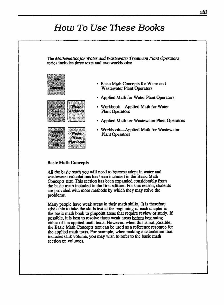
How To Use These Books
The Mathematics for Water and Wastewater Treatment Ptant Operators series includes three texts and two workbooks:
Basic Math Concepts for Water and Wastewater Plant Operators
Applied Math for Water Plant Operators - -
Workbook-Applied Math for Water
Applied Math for Wastewater Plant Operators
Plant operators
Workbook-Applied Math for Wastewater Plant operators
Basic Math Concepts
All the basic math you wil l need to become adept in water and wastewater calculations has been included in the Basic Math Concepts text. This section has been expanded considerably from the basic math included in the first edition. For this reason, students are provided with more methods by which they may solve the problems.
Many people have weak areas in their math skills. It is therefon? advisable to take the skills test at the beginning of each chapter in the basic math book to pinpoint areas that require review or study. If possible, it is best to resolve these weak areas before beginning either of the applied math texts. However, when this is not possible, the Basic Math Concepts text can be used as a reference resource for the applied math texts. For example, when making a calculation that includes tank volume, you may wish to refer to the basic math section on volumes.

Applied Math Texts and Workbooks
The applied math texts and workbooks are companion volumes. There is one set for water treatment plant operators and another for wastewater treatment plant operators. Each applied math text has two sections:
* Chapters 1 through 6 present various calculations grouped by type of math problem. Perhaps 70 percent of all water and wastewater calculations are represented by these six types. Chapter 7 groups various types of pumping problems into a single chapter. The calculations presented in these seven chapters are common to the water wastewater fields and have therefore been included in both applied math texts.
Since the calculations described in Chapters 1 through 6 represent the heart of water and wastewater matment math, if possible, it is advisable that you master these general types of calculations before continuing with other calculations. Once completed, a review of these calculations in subsequent chapters will further strengthen your math skills.
The fernaining chapters in each applied math text include calculations grouped by unit processes. The calculations are presented in the order of the flow through a plant. Some of the calculations included in these chapters are not incorporated in Chapters 1 through 7, since they do not fall into any general problem-type grouping. These chapters are particularly suited for use in a classroom or seminar setting, where the math instruction must parallel unit process instruction.
The workbooks support the applied math texts section by section. They have also been vastly expanded in this edition so that the student can build strength in each type of calculation. A detailed answer key has been provided for a l l problems. The workbook pages have been pesorated so that they may be used in a classroom setting as hand-in assignments. The pages have also been hole-punched so that the student may retain the pages in a notebook when they are returned.
The workbooks may be useful in preparing for a certification exam. However, because theses texts include both fundamental and advanced calculations, and because the requirements for each ceHication level vary somewhat from state to state, it is advisable that you fin! determine the types of problems to be covered in your exam, then focus on those types of calculations in these texts.

1
1 Applied Volume Calculations
The general equation for most volume calculations is:
Representative Depth or = [Surface Area ] [Height ]
1. Tank volume calculations. Most tank volume calculations are for tanks that are either rectangular or cylindrical in shape.
Rectangular Tank
I I JJ I I I Fflwidth, w
I 4 length,? I
Cylindrical Tank Diameter, D ’ I V = (0.785) (D2 ) (d ) I
2. Channel or pipeline volume calculations are very similar to tank volume calculations. The principal shapes are shown below.
Portion of a RectanguIar ChanneI
I* length, 1
Three general types of water and wastewater volume calculations are:
Tank Volume
Channel or Pipeline Volume
Pit, Trench, or Pond Volume
Each of these calculations is simply a specific application of volume calculations. For a mom detailed discussion of volume calculations, refer to Chapter 11 in Basic Math Concepts.
For many calculations, the volumes must be expressed in terms of gallons. To convert from cubic feet to gallons volume, a factor of 7.48 gal/cu ft is used Refer to Chapter 8 of Basic Math Concepts for a detailed discussion of cubic feet to gallons conversions.

2 Chapter 1 9 APPUED VOLUME CALCULATIONS
Portion of a Trapezoidal Channel
base,b 2 ,I
base,b
Portion of a Pipeline
.S. Diameter, D df
I V =(0 .785)(D2)(Z) I 3. Other volume calculations involving ditches or ponds
depend on the shape of the ditch or pond. A pit or trench is often rectangular in shape. A pond or oxidation ditch may have a trapezoidal cross section.


4 Cha~ter l APPLIED VOLUME CALCULATIONS
1.1 TANK VOLUME CALCULATIONS
The two common tank shapes in water and wastewater treatment are rectangular and cylindrical tanks.
Rectangular Tank:
Where:
V = Volume, cu ft l = Length, ft W =Width, ft d = Depth, ft
Cylindrical Tank:
Where:
V = Volume, cu ft D = Diameter, ft d = Depth, ft
The volume of these tanks can be expressed in cubic feet or gallons. The equations shown above are for cubic feet volume. Since each cubic foot of water contains 7.48 gallons, to convert cubic feet volume to gallons volume, multiply by 7.48 gucu ft, as illustrated in Example 2. As an alternative, you may wish to include the 7.48 gdcu ft factor in the volume equation, as shown in Example 3.
Example 1: (Tank Volume) 0 The dimensions of a tank are given below. Calculate the volume of the tank in cubic feet.
Vol., cuft = (Iw) ( d )
= (60 ft) (15 ft) (10 ft)
Example 2: (Tank Volume) Q A tank is 25 ft wide, 75 ft long, and can hold water to a depth of 10 ft. What is the volume of the tank, in gallons?
Vol., cu ft = (Iw ) (d )
= (75 ft) (25 ft) (10 ft)
= 18,750 cu ft
Now convert cu ft volume to gal:
(18,750 cu ft) (7.48 gaVcu ft) = v]
Tank Volume 5
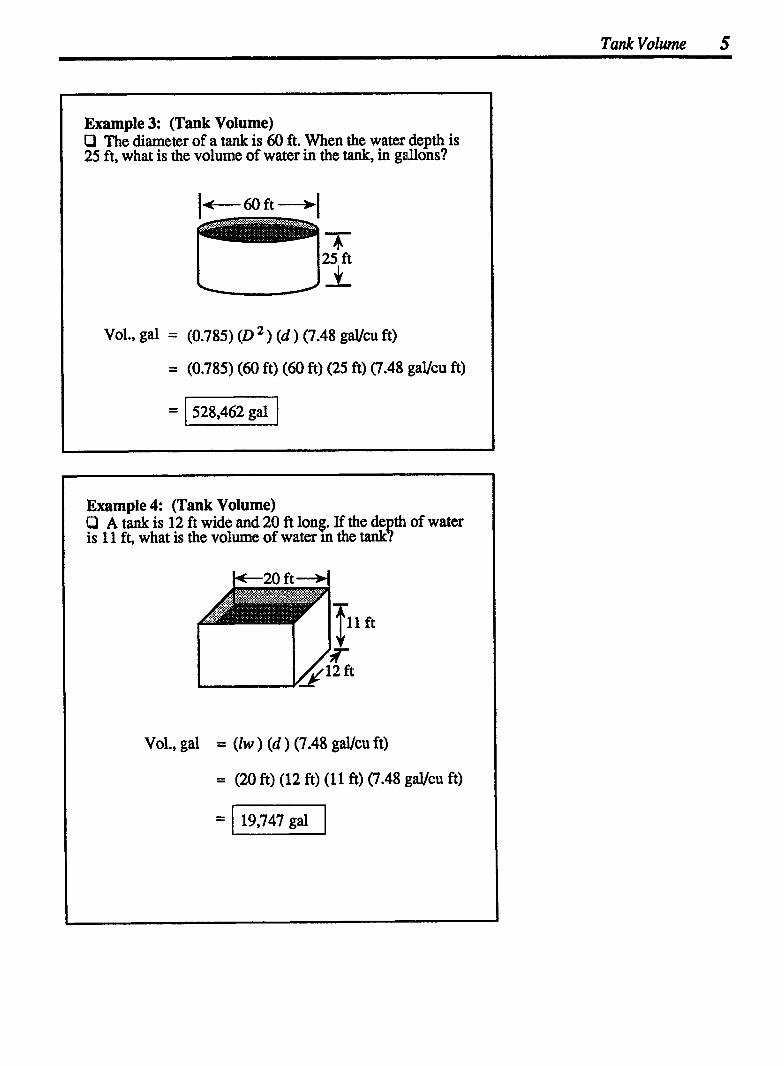
Example 3: (Tank Volume) O The diameter of a tank is 60 ft. When the water depth is 25 ft, what is the volume of water in the tank, in gallons?
vol., gal = (0.785) (D * ) (d ) (7.48 gaVcu ft)
= (0.785) (60 ft) (60 ft) (25 ft) (7.48 gaVcu ft)
= 1 528,462 gal I
Example 4: (Tank Volume) P A tank is 12 ft wide and 20 ft long. If the de th of water S is 11 ft, what is the volume of water m the tank
Vol., gal = (lw ) (d ) (7.48 gaVcu ft)
= (20 ft) (12 ft) (11 ft) (7.48 gaVcu ft)
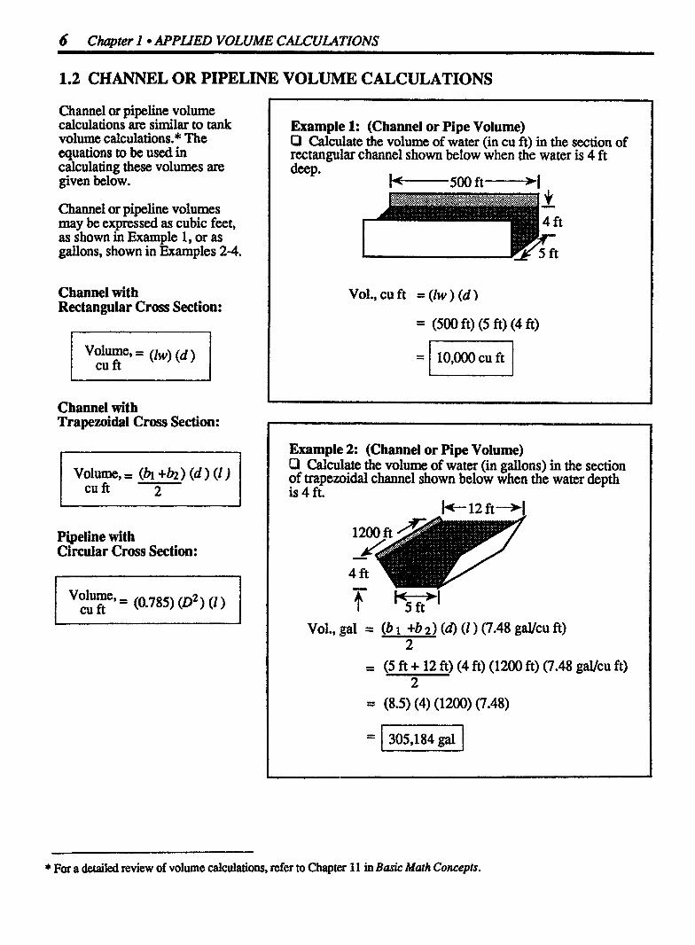
1.2 CHANNIEL OR PIPELINE VOLUME CALCULATIONS
Channel or pipeline volume calculations are similar to tank volume calculations.* The equations to be used in calculating these volumes are given below.
Channel or pipeline volumes may be expressed as cubic feet, as shown in Example 1, or as gallons, shown in Examples 2-4.
Channel with Rectangular Cross Section:
Channel with Trapezoidal Cross Section:
Volume, = (h +h ) (d ) ( I ) cu ft 2
Pipeline with Circular Cross Section:
Volume,, (0.785) (02 ) (1 )
Example l: (Channel or Pipe Volume) D Calculate the volume of water (in cu ft) in the section of rectangular channel shown below when the water is 4 ft deep.
Vol., cu ft = (lw ) (d )
= (500 ft) (5 ft) (4 ft)
Example 2: (Channel or Pipe Volume) 0 Calculate the volume of water (in gallons) in the section of trapemidal channel shown below when the water depth is 4 ft.
I t 1 2 ft--+l
= (5 ft + 12 ft) (4 ft) (1200 ft) (7.48 gdcu ft)
= ( 305,184 gal 1
* For a detailed review of volume calculations, refer to Chapter l I in Bait Math Concepts.

Channel or Pipe Vulme 7
Example 3: (Channel or Pipe Volume) D A new section of 12-inch diameter pi IPt to be disinfected before it is put into service. the length of pipeline is 2000 ft, how many gallons of water will be needed to fill the pipeline?
Vol., gal = (0.785) (D ) (l ) (7.48 gaVcu ft)
= (0.785) (1 ft) (1 ft) (2000 ft) (7.48 gaVcu ft)
Example 4: (Channel and Pipe Volume) D A section of &inch diameter pi line is to be Nled with chlorinated water for disinfection. !F 1320 ft of pipeline is to be disinfected, how many gallons of water will be required?
Vol., gal = (0.785) (D2 ) ( l) (7.48 gal/cu ft)
= (0.785) (0.5 ft) (0.5 ft) (1320 ft) (7.48 gaUcu ft)
8 Chapter l APPLJED VOLUME CALCULATIONS
1.3 OTHER VOLUME CALCULATIONS
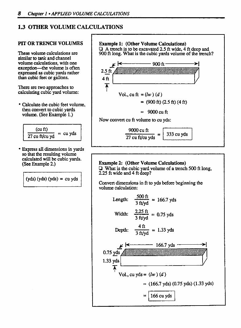
PIT OR TRENCH VOLUMES
These volume calculations are similar to tank and channel volume calculations, with one exception-the volume is often expressed as cubic yards rather than cubic feet or gallons.
There are two approaches to calculating cubic yard volume:
Calculate the cubic feet volume, then convert to cubic yards volume. (See Example 1 .)
(cu ft) 27 cu ft/cu yd = cu yds
Express all dimensions in yards so that the resulting volume calculated will be cubic yards. (See Example 2.)
Example 1: (0 ther Volume Calculations) O A trench is to be excavated 2.5 ft wide, 4 ft deep and 900 ft long. What is the cubic yards volume of the trench?
I
Vol., cu ft = (Iw ) ( d ) = (900 ft) (2.5 ft) (4 ft)
= 9000cuft
Now convert cu ft volume to cu yds:
9000 cu ft 27 cu ft/cu yds
=
Example 2: (0 ther Volume Calculations) LI What is the cubic ard volume of a trench 500 ft long, 2.25 ft wide and4 ft B eep?
Convert dimensions in ft to yds before beginning the volume calculation:
500 ft Length: - - 3 ft/ya
- 166.7 yds
Width: 2'25 ft = 0.75 y& 3 Wyd
4 ft Depth: - -
3 ft/yd - 1.33 yds
r F- 166.7 yds -1
1.33 yds I I/ +
Vol., cu yds = (Iw ) (d )
= (166.7 yds) (0.75 yds) (1.33 yds)

Other Volume Calculations 9
Example 3: (Other Volume Calculations) 0 Calculate the volume of the oxidation ditch shown below, in cu ft. The cross section of the ditch is trapezoidal.
Cross-Section - of 160 ft -1 Top View of Ditch Uitch
= (Trapezoidal) (Total Length) Area Volume
of)+ (Length Around 2 Half Circles Y
[m (4 E20 ft + (3.14) (80 ft) 1 - - 2
= p ft) (4 ftgk71.2 fg = I 18,278cuft I
Example 4: (Other Volume Calculations) 0 A ond is 5 ft deep with side slopes of 2:l (2 ft horizon- tal: 1 ! t vertical). Given the following data, calculate the volume of the pond in cubic feet.
(Top View of Pond)
550 ft*-H 570 ft-
300 ft 320 ft
v = -- 2 2
- (550 ft + 570 ft) (300 ft + 320 ft) (5 ft) - 2 2
= (560 ft) (310 ft) (5 ft)
= 1868,000 cu ft I
OXIDATION DITCH OR POND VOLUMES
Many times oxidation ditches and ponds are trapezoidal in configuration. Examples 3 and 4 illustrate these calculations.
In Example 3, the oxidation ditch has sloping sides (trapezoidal cross section). The total volume of the oxidation ditch is the trapezoidal area times the total length: Total = (bi +b2) (6) (Total Length) Vol. 2
(The total length is measured at the center of the ditch; it is equal to the length of the two straight lengths plus two half-circle lengths. Note that the length around the two half circles is equal to the circumference of one full circle.)
WHEN ALL SIDES SLOPE
In many calculations of trape- zoidal volume, such as for a tra- pezoidal channel, only two of the sides slope and the ends are vertical. To calculate the volume for such a shape, the following equation is normally used:
V = (bi + b2) (d) ( I ) fi L
Another way of thinking of this calculation is average width times the depth of water times the length :
V = (aver. width) (6) (length)
In Example 4, however, since both length and width sides are trapezoidal, the equation must include average length and average width dimensions:
I ' 2 2
-- - p -
2 Flow and Velocity CaZcuZcttions
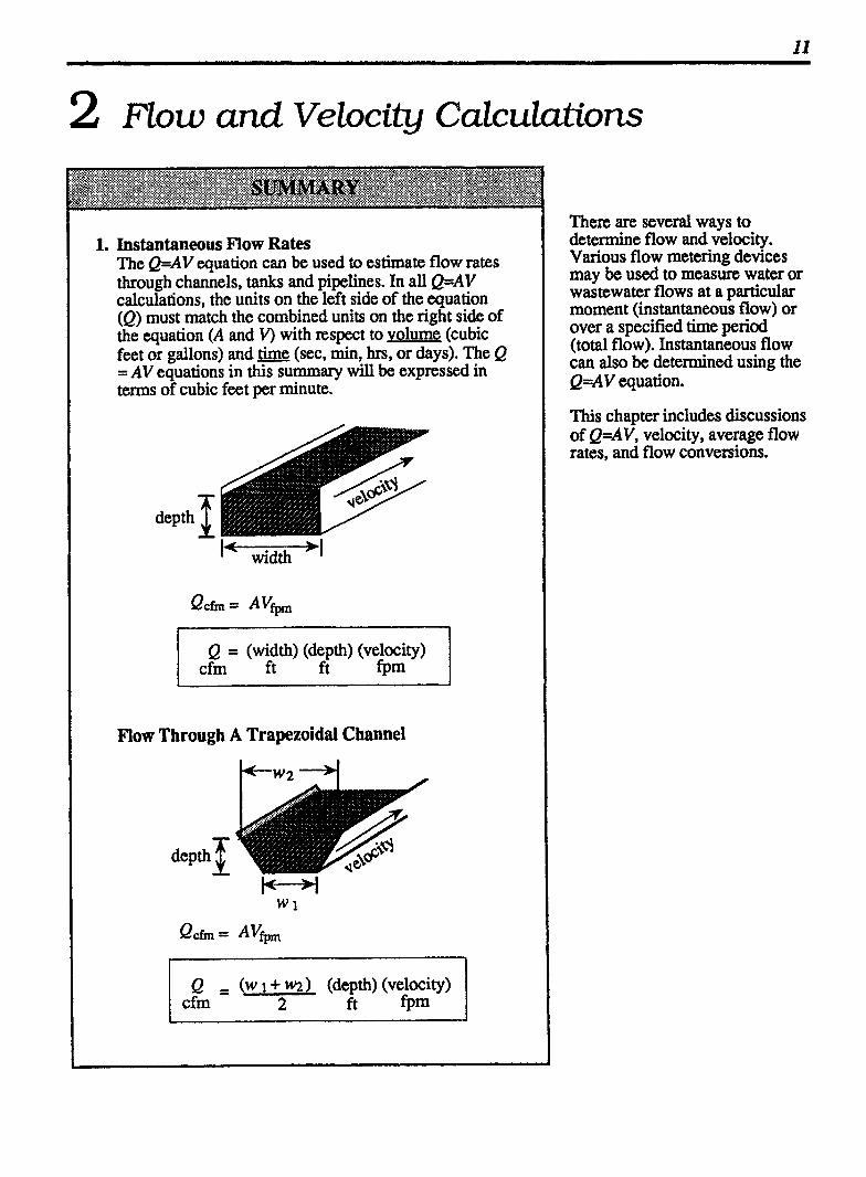
1. Instantaneous Flow Rates The Q=AV equation can be used to estimate flow rates through channels, tanks and pipelines. In all Q=AV calculations, the units on the left side of the equation (Q) must match the combined units on the right side of the equation (A and V) with respect to volumq (cubic feet or gallons) and ~ime (sec, min, hrs, or days). The Q = AV equations in this summary will be expressed in terms of cubic feet per minute.
Flow Through A Trapezoidal Channel
I
Q = (W 1 + tc2 1 (depth) (velocity) 2 ft fpm
Q = (width) (depth) (velocity) cfm ft ft fP
i
There are several ways to determine flow and velocity. Various flow metering devices may be used to measure water or wastewater flows at a particular moment (instantaneous flow) or over a specified time period (total flow). Instantanwus flow can also be determined using the Q=AV equation.
This chapter includes discussions of Q=AV, velocity, average flow rates, and flow conversions.
12 Chapter 2 FLOW AND VEWCITY CALCULATIONS
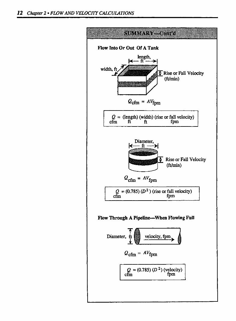
Flow Into Or Out Of A Tank
width Rise or Fall Velocity (ft/min)
I I/
Q = (length) (width) (rise or fall velocity) cfm ft ft fpm
Diameter, L f t + I
Rise or Fall Velocity (Wmin)
Q = (0.785) (D ) (rise or fall velocity) I cfm fpm
Flow Through A Pipeline-When Flowing Full
T L
Diameter, ft
Q = (0.785) (D 2, (velocity) fpm

13
I
Flow Through A Pipeline--When Flowing When Less Than Full
f Diy depth
1
Q = (new) (D *) (velocity)
*Based on 4D Table
cfm factor fpm +
2. Velocity Calculations The Q=AV equation can be used to determine the velocity of water at a particular moment. Use the same Q=AV equation, fdl in the known information, then solve for velocity.
Distance Traveled, ft Duration of Test, min
Velocity =
Velocity = - xnin
The Q=AV equation can also be used to detemnine velocity changes due to differences in pipe diameters. The AV in one pipe is equal to the AV in the other pipe.
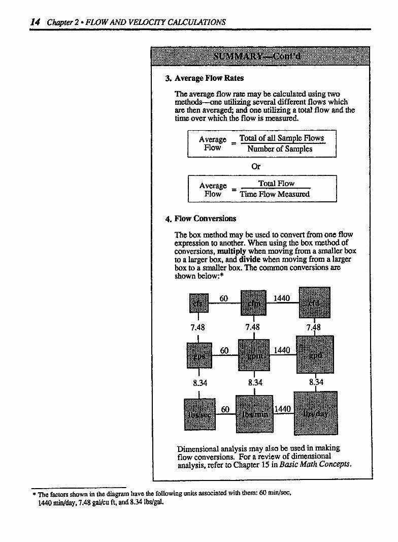
3. Average Flow Rates
The average flow rate may be cdiculated using two methods-one utilizing several different flows which are then average& and one utilizing a total flow and the time over which the flow is measured
Average - Total of all Sample HOWS - Number of Samples
or Average - Total Flow - Flow Time How Measured
4. Flow Conversions
The box method may be used to c o n v e ~ fkom one flow expression to another. When using the box method of conversions, multiply when moving from a smaller box to a larger box, and divide when moving from a larger box to a smaller box. The common conversions axe shown below:*
7.48 7.48
8.34 8.34 8.34
Dimensional analysis may also be used in making flow ~onv~rsions* For a review of ~ m ~ n s ~ o n ~ analysis, refer to Chapter 15 in Basic Math Concepts.
* The fs&ors shown in the diagram have the follo~ing uni& associated with them: 60 ~ i ~ s ~ , 1440 min/day, 7.48 gal/cu ft, and 8.34 Wgd.


I 6 Chupter 2 FLOW AND VELOCITY CALCULATIONS
2.1 INSTANTANEOUS FLOW RATES CALCULATIONS
The flow rate through channels and pipelines is normally measured by some type of flow metering device. However the flow rate for any particular moment can also be determined by using the Q=AV equation.
The flow rate (Q) is equal to the cross-sectional area (A) of the channel or pipeline multiplied by the velocity through the channel or pipebe. There are two important considerations in these cdtcdations:
1. Remember that volume is calculated by multiplying the representative area by a third dimension, often depth or height* The Q=AV calculation is essentially a volume calculation. The length dimension is a velocity m (lengthhime):
Vole (Cross. Sectional) (3rd Dim.) Area - -
2. The units used for volume and time must be the same on both sides of the equation, as shown in the diagram to the right.
FLOW THROUGH A RECTANGULARCHANNEL
The principal difference among various Q=AV calculations is the shape of the cross-sectional area Channels normally have rectangular or trapezoidal cross sections, whereas pipelines have circular cross sections. Examples 1-3 illustrate the Q=AV calculation when the channel is rectangular.
&AV CfiCULAIONS ARE ESSENTMLL,Y VOLUME CALCULATIONS WITH A TlME CONSIDERATION
A,
width *I
Q = A V cu ft/time (ft) (ft) (ft/time)
IN ALL Q=AV EQUATIONS, VOLUME AND TIME UNITS MUST MATCH
e = A V cu ft/min ,(ft) (ft) (ft!min)
Example 1: (Instantaneous Flow) P A channel 3 ft wide has water flowin to a depth of
the cfs flow rate through the channel? f 2.5 ft. If the velocity through the channe is 2 @S, what is
= (3 ft) (2.5 ft) (2 fps)
* For a review of volume dculations, refer to Chapter 11 in Basic Math Concepts.

Instantaneous Flow Rates 17
Example 2: (Instantaneous Flow) O A channel 40 inches wide has water flowing to a of 1.5 ft. If the velocity of the water is 2.3 $S, what cfs flow in the channel?
Qcfs = &fps
= (3.3 ft) (1.5 ft) (2.3 +S)
Example 3: (Instantaneous Flow) O A channel 3 ft wide has water flowing at a velocity of 1.5 fps. If the flow through the channel is 8.1 cfs, what is the depth of the water?
xft f -
Qcfs = AVfps
8.1 cfs = (3 ft) (X ft) 1.5 @S)
8, l (3) (1.5)
= xft
DIMENSIONS SHOULD BE EXPRESSED AS FEET
The dimensions in a Q=AV calculation should always be expressed in feet because (ft) (ft) (ft) = cu ft. Therefore, when dimensions are given as inches, first convert all dimensions to feet before beginning the Q=AV calculation.
Note that velocity may be written in either of two forms:
fps or fpm ft/sec or ft/min
The first form is shorter. The second form is usefbl when dimensional analysis* is desired
CALCULATmG OTHER UNKNOWN VARIABLES
There are four variables in Q=AV calculations for rectangular channels: flow rate, width, depth, and velocity. In Examples 1 and 2, the unknown variable was flow rate, Q. However, any of the other variables can also be unknown. * *Example 3 illustrates a calculation when depth is the unknown factor, Section 2.2 of this chapter illustrates calcula- tions when velocity is the un- known factor.
* The concept of dimensional analysis is discussed in Chapter 15 in Basic Math Concepts. * * For a review of solving for the unknown variable, refer to Chapter 2 in Basic Math Concepts. These type
problems are primarily theoretical, since channel size is normally a given and water depth is measured.
I 8 Chapter 2 * FLOW AND V E U ) C m CALCULATIONS
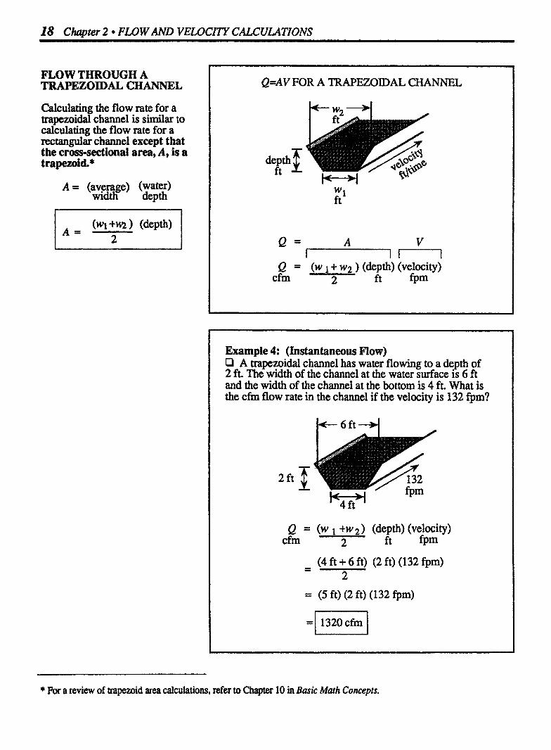
FLOW THROUGH A TRAPEZOlDAL CHAIVNL
Calculating the flow rate for a trapezoidal channel is similar to calculating the flow rate for a rectangular channel except that the cross-sectional area, A, is a t rapemid.*
A = (average) (water) width depth
Q = (W 1 + wz ) (depth) (velocity) cfm 2 ft fpm
Example 4: (instantaneous Flow) Q A trapezoidal channel has water flowing to a depth of 2 ft. The width of the channel at the water surface is 6 ft and the width of the channel at the bottom is 4 ft. What is the cfm flow rate in the channel if the velocity is 132 f p ?
Q = (W 1 +W 2 ) (depth) (velocity) cfm 2 ft fpm
- - (4 ft + 6 ft) (2 ft) (132 fpm) 2
= (5 ft) (2 ft) (132 $m)
* For a review of trapezoid area calculations, refer to Chapter 10 in Basic Math Concepts.

Instantaneous Flow Rates 19
Example 5: (Instantaneous Flow) P A trapezoidal channel is 3 ft wide at the bottom and 5.5 ft wide at the water surface. The water depth is 30 inches. If the flow velocity through the channel is 168 ft/rnin, what is the cfm flow rate through the channel?
30 in. - = 2.5 f t x 12 in./ft
Q = (W 1 +W 2) (depth) (velocity) cfm 2 ft fpm
- - (3 ft + 5.5 ft) (2.5 ft) (168 fpm) 2
=l 1785 cfm I
Example 6: (Instantaneous Flow) Q A trapezoidal channel has water flowin to a depth of % 16 inches. The width of the channel at the ottom is 3 ft and the width of the channel at the water surface is 4.5 ft. If the velocity of flow through the channel is 2.5 ft/sec, what is the cfm flow through the channel?
16 in. 12 in./ft
= 1.3 ft$
First calculate the flow rate that matches the velocity time frame:
(3 ft + 4.5 ft) (1.3 ft) (2.5 fps) Q = 3 cfs L
= 12.2 cfs Now convert cfs flow rate to cfm flow rate:
(12.2 cfs) (60 sec) = ( 732 cfm I min
WHEN DATA IS NOT GIVEN IN DESIRED TERMS
Many times the data to be used in a Q=AV equation is not in the form desired. For example, dimensions might be given in inches rather than in feet, as desired. Or perhaps the velocity is expressed as fps yet the flow rate is desired in cfm. (The time element does not match- seconds vs. minutes.) These type calculations are illustrated in Examples 5 and 6.
When the velocity and flow rate time frames do not match, you must convert one of the terms to match the other.
Since flow rate conversions are quite common, you may find it easiest to leave the velocity ex- pression as is and then convert the flow rate to match the velocity time fiame. Example 6 illustrates such a process.

20 Chapter 2 FLOW AND VELOCITY CALCULATIONS
FLOW INTO A TANK
Flow through a tank can be considend a type of Q=AV calculation.* If the discharge valve to a tank were closed, the water level would begin to rise. Timing how fast the water rises would give you an indication of the velocity of flow into the tank. The Q=AV equation could then be used to determine the flow rate into the tank, as illustrated in Example 7.
If the influent valve to the tank were closed, rather than the discharge valve, and a pump continued discharging water from the tank, the water level in the tank would begin to drop. The rate of this drop in water level could be timed so that the velocity of flow from the tank could be calculated. Then the Q=AV equation could be used to determine the flow rate out of the tank, as illustrated in Example 8.
Example 7: (Instantaneous Flow) P A tank is 12 ft by 12 ft. With the discharge valve closed, the influent to the tank causes the water level to rise 1.25 feet in one minute. What is the gpm flow into the tank?
First, calculate the cfm flow rate:
= (12 ft) (12 ft) (1.25 @m)
= 180 cfm Then convert cfm flow rate to gpm flow rate:
(1 80 cfm) (7.48 gdcu ft) = -1
Example 8: (Instantaneous Flow) P A tank is 8 ft wide and 10 ft long. The influent valve to the tank is closed and the water level drops 2.8 ft in 2 minutes. What is the gpm flow from the tank?
Jt-10 ft --+I
2 rnin - - J.
First, calculate the cfm flow rate:
Qcfm = AVfpm
= (10 ft) (8 ft) (1.4 fpm)
= 112 cfm Then convert cfm flow rate to gpm flow rate:
(1 12 cfm) (7.48 gal/cu ft) = 838 gprn ti * This is the same type of calculation described in Chapter 7 as pump capacity calculations.
Instantaneous Flow Rates 21
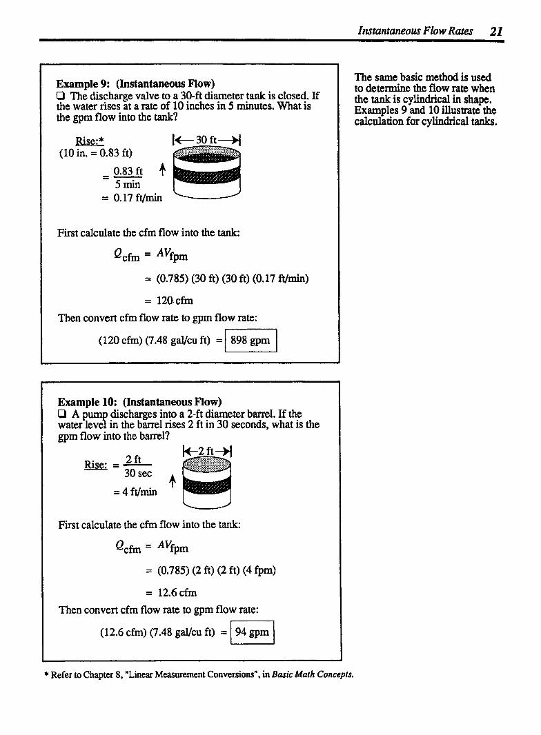
Example 9: (Instantaneous Flow) Cl The discharge valve to a 30-ft diameter tank is closed. If the water rises at a rate of 10 inches in 5 minutes. What is the gpm flow into the tank?
Rise:* (10 in. = 0.83 ft)
0.83 ft -- - 5 min
First calculate the cfrn flow into the tank:
l = (0.785) (30 ft) (30 ft) (0.17 Nmin)
= 12O.cfm
1 Then convert cfrn flow rate to gpm flow rate:
(120 cfm) (7.48 gacu ft) = 898 gprn U
Example 10: (Instantaneous Flow) Ll A pum discharges into a 2-ft diameter b m l . If the water leve 7 in the barrel rises 2 ft in 30 seconds, what is the gpm flow into the barrel? r
2 ft Rise; = - 30 sec
= 4 ft/min +
I First calculate the cfm flow into the tank:
= (0.785) (2 ft) (2 ft) (4 fpm)
I = 12.6 cfrn
1 Then convert cfrn flow rate to gpm flow rate:
(12.6 cfm) (7.48 gal/cu ft) = 1 94 gprn I
The same basic method is used to determine the flow rate when the tank is cylindrical in shape. Examples 9 and 10 illustrate the calculation for cylindrical tanks.
* Refer to Chapter 8, "Linear Measurement Conversionsn, in Basic Math Concepts.

22 Chapter 2 FLOW AND VELOCITY CALCULATIONS
FLOW THROUGH A PIPELINE--WHEN FLOWING FULL
The flow rate through a pipeline can be calculated using the Q=AV equation. The cross- sectional area is a circle, so the area, A, is represented by (0.785) (D*). Pipe diameters should generally be expressed as feet to avoid errors in terms.
Q=AV CALCULATIONS FOR A PIPELINE FXOWING FULL
T Diam., ft 1
Q cfs =
Example 11: (Instantaneous Flow) Cl The flow through a 6-inch diameter pipeline is moving at a velocity of 3 ftlsec. What is the cfs flow rate through the pipeline? (Assume the pipe is flowing full.)
Qcfs = AV@s
= (0.785) (0.5 ft) (0.5 ft) (3 fps)

Instantaneous Flow Rates 23
Example 12: (Instantaneous Flow) O An 8-inch diameter pipeline has water flowing at a velocity of 3.4 @S. What is the gpm flow rate through the pipeline?
First, calculate the cfs flow rate:
Qcfs = AVis
= (0.785) (0.67 ft) (0.67 ft) (3.4 f p s )
= 1 .2 cfs
Then convert cfs flow rate to gpm flow rate:
(1.2 - cu ft) (60 sec) (7.48 - sec min cu ft
Example 13: (Instantaneous Flow) O The flow through a pipeline is 0.7 cfs. If the velocity of flow is 3.6 ft/sec and the pipe is flowing full, what is the diameter (inches) of the pipeline?
< - X ft &$$ I?lowRate
t* i8 = 0.7 cfs
First calculate the diameter in feet:
Qcfs = AVfp
0.7 cfs = (0.785) (x2 sq ft) (3.6 fps)
Now convert feet to inches: - (0.5 ft) (12 - in.) =l 6 inches1
SOLVING FOR OTHER UNKNOWN VARIABLES
There are three variables in Q=AV calculations for pipelines: flow rate (Q), diameter (D), and velocity (V). In Examples 11 and 12, the unknown factor is flow rate. In Example 13, the unknown factor is pipeline dia- meter. (Section 2.2 illustrates calculations when velocity is the unknown variable.)
When the diameter is the unknown variable, first solve for x ? Then, by taking the square root* of both sides of the equation, x may be determined.
* For a review of square roots, refer to Chapter 13 in Basic Math Concepts.

24 Chapter 2 FLOW AND VEWCITY CALCULATIONS
FLOW THROUGH A PIPELINE--WHEN FLOWING LESS THAN FULL
Calculating the flow rate through a pipeline flowing less than full is similar to calculating the flow rate for a pipeline flowing full with one exception-instead of using 0.785 as a factor in the area calculation, a different factor is used. This factor is based on the ratio of water depth (d) to the pipe diameter (D). Calculate the dlD value, then use the table to determine the factor to be used instead of 0.785.
WHEN MAKING Q=AV CALCULATIONS FOR A PIPELINE FLOWING LESS THAN FULL
-A DIFFERENT FACTOR THAN 0.785 IS USED
t Diam., ft
L Q cfs = A
neter Table
Ble Factor
0.76 0.6404 0.77 0.6489 0.78 0.6573 0.79 0.6655 0.80 0.6736

Instantaneous Flow Rates 25
Example 14: (Instantaneous Flow) Cl The flow through a 6-inch diameter ipeline is moving K at a velocity of 3 ft/sec. If the water is owing at a depth of 4 inches, what is the cfs flow rate through the pipeline?
First use the dD ratio to determine the factor to be used instead of 0.785 in the Q=AV calculation:
The factor shown in the table corresponding to a dlD of 0.67 is 0.5594. Now calculate the flow rate using Q=AV:
Qcfs = e f p s
= (0.5594) (0.5 ft) (0.5 ft) (3 fps)
=/0.42 cfs I
Example 15: (Instantaneous Flow) LI An 8-inch diameter pipline has water flowing at a velocity of 3.4 fps. What is the gpm flow rate through the pipeline if the water is flowing at a depth of 5 inches?
fl = 0.67 ft 5 in .: 3.4 fps S '. .
First, determine the factor to be used instead of 0.785. Since dlD=0.63, the factor listed in the table is 0.5212. Now calculate the flow rate using Q=AV. Although gpm flow rate is desired, first calculate cfs flow rate, then convert cfs to gpm flow rate:
Qcfs = AVfps = (0.5212) (0.67 ft) (0.67 ft) (3.4 @S)
= 0.8 cfs
Then convert cfs flow rate to gpm flow rate:
(0.8 - cu ft) (60 - sec) (7.48pJ = sec min cu ft
Examples 14 and 15 illustrate use of the Q = AV equation when the pipeline is flowing less than full.
26 Chapter 2 FLOW AND VELOCITY CUCULATIONS
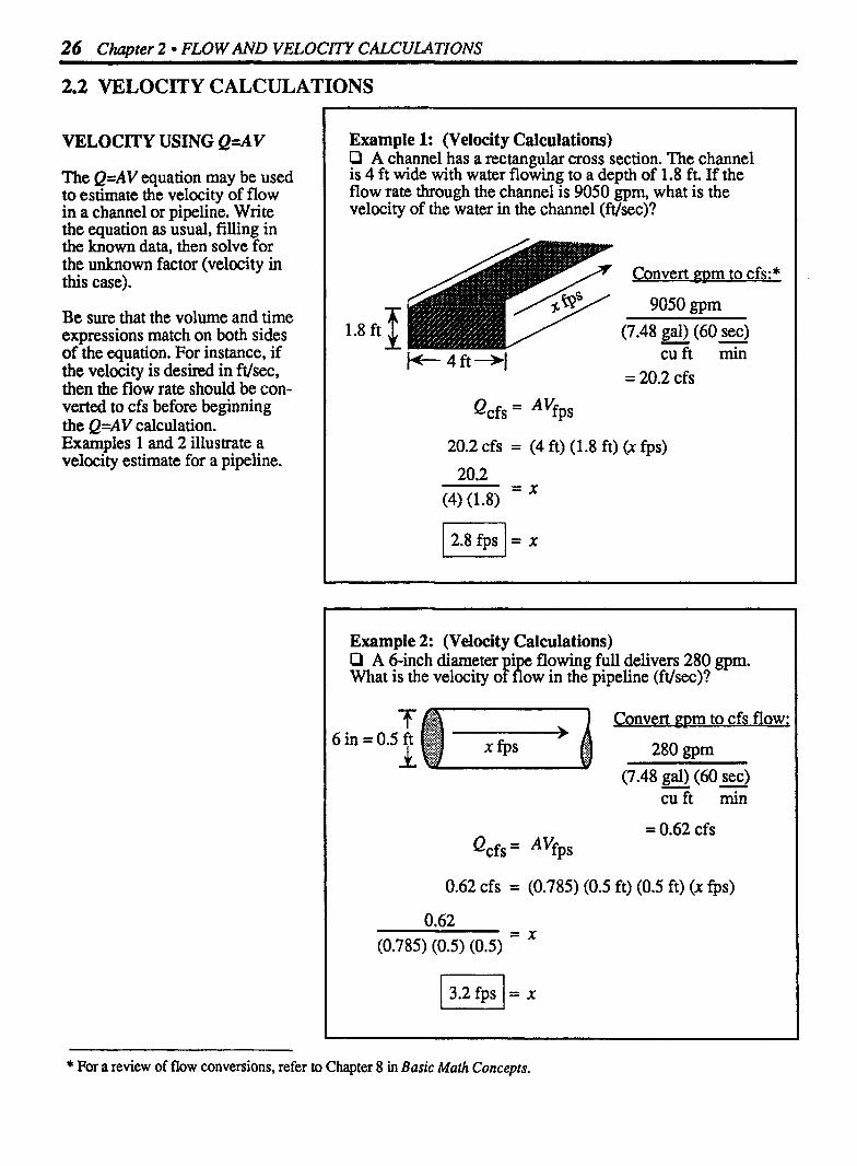
2.2 VELOCITY CALCULATIONS
VELOCITY USING Q=AV
The Q=AV equation may be used to estimate the velocity of flow in a channel or pipeline. Write the equation as usual, filling in the known data, then solve for the unknown factor (velocity in this case).
Be sure that the volume and time expressions match on both sides of the equation. For instance, if the velocity is desired in ft/sec, then the flow rate should be con- verted to cfs before beginning the Q=AV calculation. Examples 1 and 2 illustrate a velocity estimate for a pipeline.
Example 1: (Velocity Calculations) O A channel has a rectangular cross section. The channel is 4 ft wide with water flowing to a depth of 1.8 ft. If the flow rate through the channel is 9050 gpm, what is the velocity of the water in the channel (ft/sec)?
Convert m m to cfs: * 9050 gpm
1.8 ft 1 (7.48 gal) (60 sec) - - cu ft min .
= 20.2 cfs
Qcfs = AVfps
20.2 cfs = (4 ft) (1.8 ft) (X fps)
Example 2: (Velocity Calculations) Q A 6-inch diameter i flowing full delivers 280 gpm. What is the velocity o!gw in the pipeline (ft/sec)?
Convert m m to cfs flow;
280 gpm (7.48 gal) (60 sec) - -
iu ft min
= 0.62 cfs Qcfs = AVfp
0.62 cfs = (0.785) (0.5 ft) (0.5 ft) (X @S)
* For a review of flow conversions, refer to Chapter 8 in Basic Moth Concepts.

Velocity Calculations 27
r 1
2 min 14 sec = 134 sec
velocity - Distance, ft ft/sec Time, sec
-
- 300 ft - 134 sec
Example 4: (Velocity Calculations) 0 A fluorescent dye is used to estimate the velocity of flow in a sewer. The dye is injected in the water at one manhole and the travel time to the next manhole 400 ft away is noted. The dye first appears at the downstream manhole in 128 seconds. The dye continues to be visible until a total elapsed time of 148 seconds. What is the ft/sec velocity of flow through the pipeline?
Dye injected Manhole 2
J.
I 4ooft-I
First calculate the average travel time of the dye:
128 sec + 148 sec = 138 sec L
Then calculate the ft/sec velocity:
Velocity = 400 ft ft/sec 138 sec
VELOCITY USING THE FLOAT OR DYE METHOD
The Q = AV calculation estimates the theoretical velocity of flow in a channel or pipeline. Actual velocities in the pipeline can be measured by metering devices. Velocities can also be estimated by the use of a float or dye placed in the water. Then, by timing the distance traveled using a float or dye, the velocity of flow can be determined:
Velocity _. Distance, ft ft/sec - Time, sec
A float is perhaps less accurate in estimating velocities in a pipeline than use of fluorescent tracer dyes. In channels, floats move along with the faster surface waters and can be as much as 10 or 15 percent faster than the actual average flow rate. Some floats designed for use in channels include segments that extend into the water, thus responding to a moR average velocity through the channel.
In pipelines, floats can become entangled or slowed down by obstructions.
Tracer dyes tend to give a better estimate of velocity. Since some of the dye will travel faster and some slower, you will need to determine the average time required to travel from one point to the next. To calculate the average time for travel:

28 Chapter 2 FU)W AND VELOCITY CALCULATIONS
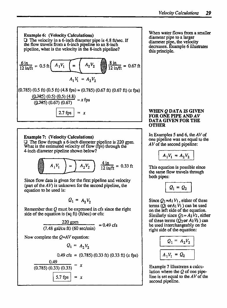
USING Q=AV TO ESTIMATE CHANGES IN VELOCITY
In addition to estimating flow in a channel or pipeline, the Q=AV equation can be used to estimate the change in velocity as the water flows from one diameter pipeline to another.
When water flows from a larger diameter pipe to a smaller dia- meter pipe, the velocity in- creases. (The water must move faster since the same amount of water is flowing through a smaller space.) Example 5 illustrates this calculation.
FLOW RATE (Q) IN PIPES REMAIN CONSTANT
Since the total flow in the pipeline must remain constant:
Q1 = Q2
AIVl = A2V2
Example 5: (Velocity Calculations) Q The velocity in a 12-inch diameter pipeline is 3.8 ft/sec. If the 12-inch pipeline flows into a 10-inch diameter pipeline, what is the velocity in the 10-inch pipeline?
1 -3 \ in:,
(0.785) (1 ft) (1 ft) (3.8 fps) = (0.785) (0.83 ft) (0.83 ft) (X @S)
(8-785) (1) (1) (3.8) (lM83) (0.83) (0.83) = xfps
Velocity Calculations 29
Example 6: (Velocity Calculations) LI The velocity in a 6-inch diameter pipe is 4.8 ft/sec. If the flow travels from a dinch pipeline to an 8-inch pipeline, what is the velocity in the 8-inch pipeline?
l(0.785) (0.5 ft) (0.5 ft) (4.8 fps) = (0.785) (0.67 ft) (0.67 ft) (X @S)
-
Example 7: (Velocity Calculations) Q The flow through a 6-inch diameter ipeline is 220 gpm. What is the estimated velocity of flow &S) through the 4-inch diameter pipeline shown below?
Since flow data is given for the fust pipeline and velocity (part of the AV) is unknown for the second pipeline, the equation to be used is:
Remember that Q must be expressed in cfs since the right side of the equation is (sq ft) (ft/sec) or cfs:
220 Rpm = 0.49 cfs
(7.48 gal/cu ft) (60 sechin)
Now complete the Q=AV equation:
0.49 cfs = (0.785) (0.33 ft) (0.33 ft) (X @S)
When water flows from a smaller diameter pipe to a larger diameter pipe, the velocity decreases. Example 6 illustrates this principle.
WHEN Q DATA IS GIVEN FOR ONE PIPE AND AV DATA GIVEN FOR THE OTHER
In Examples 5 and 6, the AV of one pipeline was set equal to the A V of the second pipeline:
This equation is possible since the same flow travels through both pipes:
Since Q1 =A1 V1 , either of these terms (0 orAi V1 ) can be used on the left side of the equation. Similarly since Q2 = A2 V2 , either of these terms (Qzor A2 Vi ) can be used interchangeably on the right side of the equation:
Example 7 illustrates a calcu- lation where the Q of one pipe- line is set equal to the AV of the second pipeline.

30 Chopter 2 FLOW AND VEWCITY CALCULATIONS
2.3 AVERAGE n o w RATES CALCULATIONS
Flow rates in a treatment system may vary considerably during the course of a day. Calculating an average flow rate is a way to detemine the typical flow rate for a given time h e such as: average daily flow, average weekly flow, average monthly flow, or even average yearly flow.
There are two ways to calculate an average flow rate. In the f ~ s t method, several flow rate values are used to determine an average value, as illustrated in Examples 1 and 2.
Average = Tot. of all Sample Flows No. of Samples
In the second method, a total flow is used (from a totalizer reading) to determine an average flow rate. Examples 3 and 4 illustrate this type of calculation.
Average Tot. Flow from Totalizer Flow Time Over Which
Flow Measud
Example 1: (Average Flow Rates) O The followin flows were recorded for the week:
h f Monday-86 GD; Tuesday-7.6 MGD; Wednes- day-7.2 MGD; Thursday-7.8 MGD; Friday-8.4 MGD; Saturday-8.6 MGD; Sunday-7.5 MGD. What was the average daily flow for the week?
Total of all Sample Flows Average Daily Flow =
Number of Days
- - 55.7 MGD 7 Days
Example 2: (Average Flow Rates) P The following flows were ncorded for the months of September, October and November: September-1 20.8 MG; October- 136.4 MG; November-156.1 MG. What was the average daily flow for this three-month period?
Since average daily flow is desired, you must divide by the number of days represented by the three-month period, rather than by the number of months represented. (If average monthly flow had been desired, then you would divide by the number of months represented.)
Total of all Sample Flows Average Daily Flow =
Number of Days
- - 413.3 MG 91 days
Average Flow Rates 31
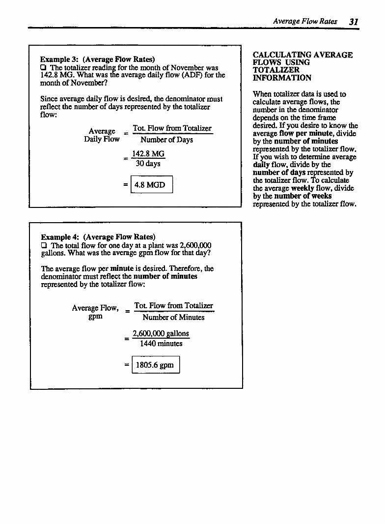
Example 3: (Average Flow Rates) O The totalizer readin for the month of November was
t% 142.8 MG. What was e average daily flow (ADF) for the month of November?
Since average daily flow is desired, the denominator must reflect the number of days represented by the totalizer flow:
Average = Tot. How fiom Totalizer Daily Flow Number of Days
- - 142.8 MG 30 days
Example 4: (Average Flow Rates) Cl The total flow for one day at a plant was 2,600,000 gallons. What was the average gpm flow for that day?
The average flow per minute is desired. Therefore, the denominator must reflect the number of minutes represented by the totalizer flow:
Average low, - Tot. Flow from Totalizer - Number of Minutes
2,600.000 gallons 1440 minutes
CALCULATING AVERAGE FLOWS USING TOTALIZER INFORMATION
When totalizer data is used to calculate average flows, the number in the denominator depends on the time W e desired. If you desire to know the average flow per minute, divide by the number of minutes represented by the totalizer flow. If you wish to determine average daily flow, divide by the number of days repsented by the totalizer flow. To calculate the average weekly flow, divide by the number of weeks represented by the totalizer flow.
32 Chapter 2 FLOW AND VELOCITY CALCULATIONS
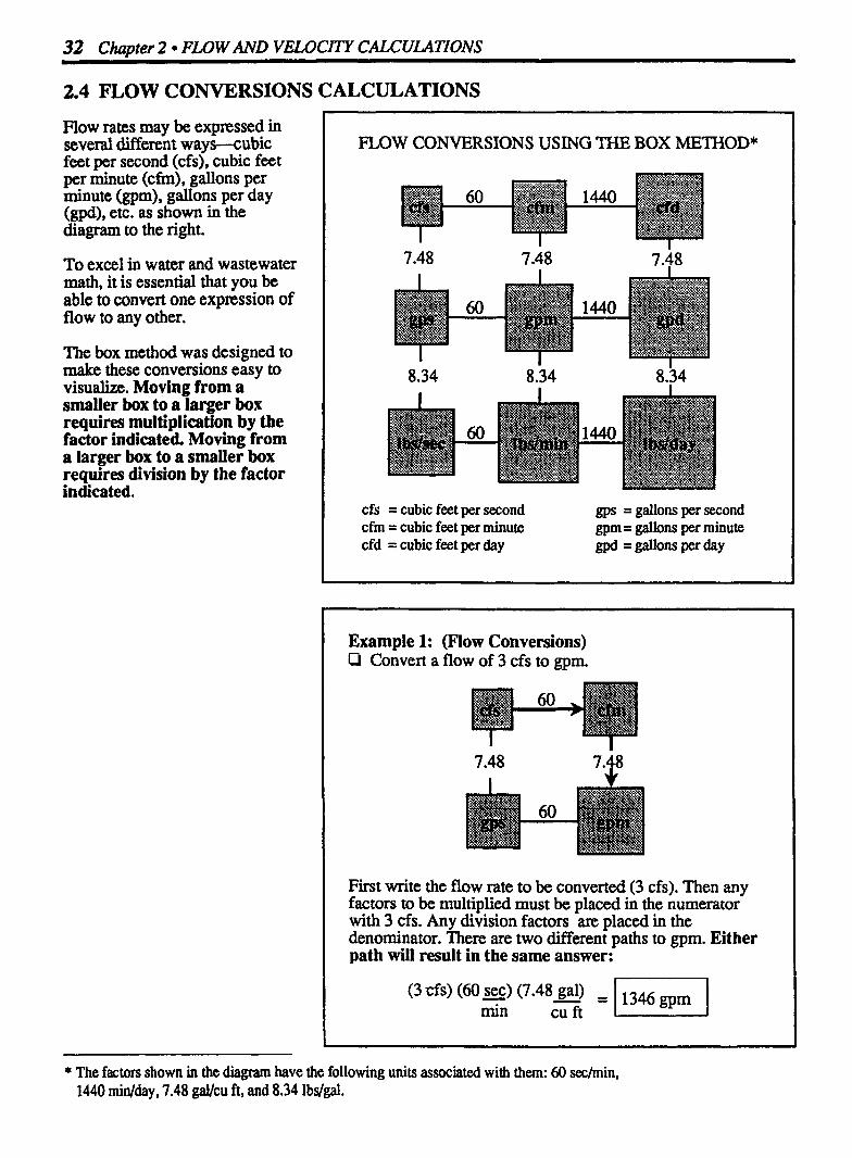
2.4 n o w CONVERSIONS CALCULATIONS
Flow rates may be expressed in several different way ~ u b i c feet per second (cfs), cubic feet per minute (cfm), gallons per minute (gpm), gallons per day (gpd), etc. as shown in the diagram to the right.
To excel in water and wastewater math, it is essential that you be able to convert one expression of flow to any other.
The box method was designed to make these conversions easy to visualize. Moving from a smaller box to a larger box requires multiplication by the factor indicated Moving from a larger box to a smaller box requires division by the factor indicated.
FLOW CONVERSIONS USING THE BOX METHOD*
cfs = cubic feet per second gps = gallons per second cfm = cubic feet per minute gpm = gallons per minute cfd = cubic feet per day gpd = gallons per day
Example 1: (Flow Conversions) C1 Convert a flow of 3 cfs to gpm.
First write the flow rate to be converted (3 cfs). Then any factors to be multiplied must be placed in the numerator with 3 cfs. Any division factors are placed in the denominator. There are two different paths to gpm. Either path will result in the same answer:
(3 cfs) (6O (7m48 gal) = [ 1346 gpm 1 min c u t
* The factors shown in the diagram have the following units associated with them: 60 &min. 1440 min/day ,7.48 gdcu ft, and 8.34 lbdgal.

Flow Conversions 33
Example 2: (Flow Conversions) O Convert a flow of 45 gps to d. Use dimensional P analysis to check the set up of e problem.
Write the flow rate to be converted, then place multiplication or division factors in the numerator or denominator, as required:
Now use dimensional analysis to check the math set up of this problem:
Example 3: (Flow Conversions) O Convert a flow of 3,200,000 gpd to cfm. Use dimensional analysis to check the set up of the problem.
Two different paths may be used from gpd to cfm. Either path will result in the same answer:
3,200,000 gpd (1440 &n) (7.48 gal)
=F1 Now use dimensional analysis to check the math set up of this problem:*
day - A y @ cu ft cu ft - a = -
min @ g a l Aaf min 4 min day cu ft
USING DIMENSIONAL ANALYSIS TO CHECK THE MATH SET UP
Dimensional analysis is often used to check the mathematical set up of conversions. Examples 2 and 3 illustrate how to use dimensional analysis in checking the problem set up. Refer to Chapter 15 in Basic Math ~once$s for a fimher discussion of dimensional analysis.
QUICK CONVERSIONS
There are two conversion equations used quite fi-equently in water and wastewater treatment calculations. You would be well advised to memorize these equations for use in quick conversions:
1 MGD = 1.55 cfs 1 MGD = 694 gpm r
Should you forget these numbers, you can always derive them yourself using the box method of conversions.
* For a review of corn~lex fractions, refer to Cha~ter 3 in Basic Math Concepts.

3 Milligrams per Liter to Pounds per Day Calculations
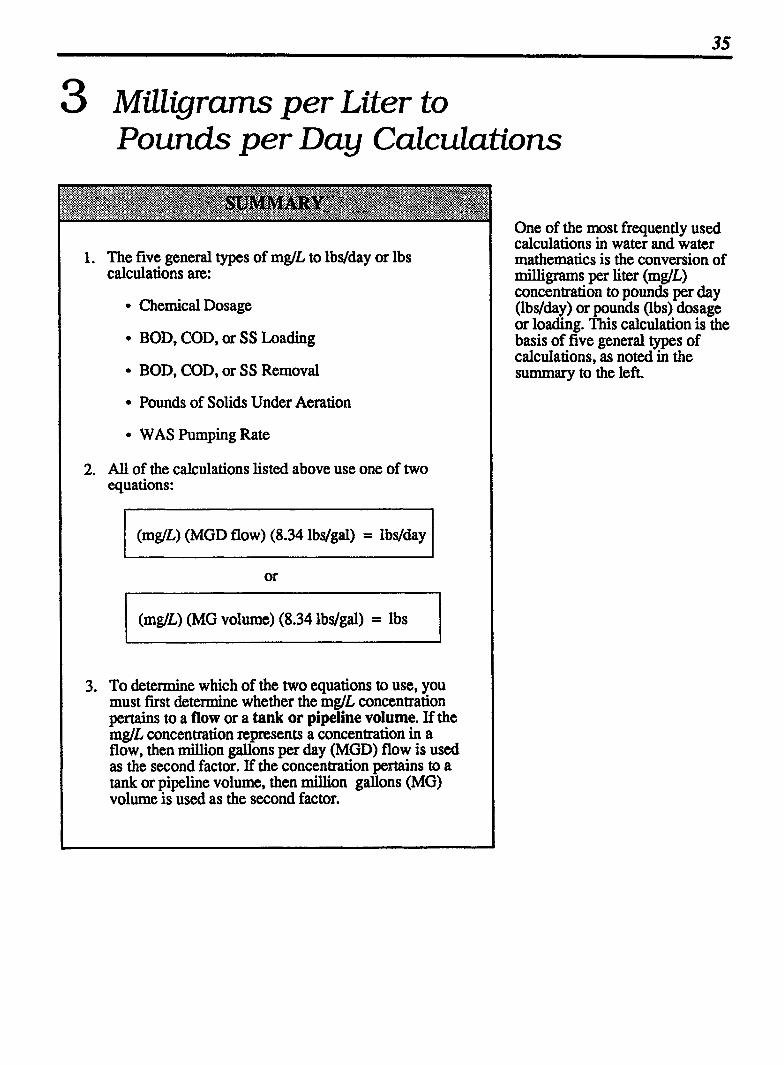
1. The five general types of m& to lbs/day or lbs calculations are:
Chemical Dosage
BOD, COD, or SS Loading
BOD, COD, or SS Removal
Pounds of Solids Under Aeration
WAS Pumping Rate
2. All of the calculations listed above use one of two equations:
l
(rng/L) (MGD flow) (8.34 lbdgal) = Ibs/day
I (mglL) (MG volume) (8.34 lbdgal) = lbs
3. To determine which of the two equations to use, you must first determine whether the mglL concentration pertains to a flow or a tank or pipeline volume. If the mg/L concentration represents a concentration in a flow, then million gallons per day (MGD) flow is used as the second factor. If the concentration pertains to a tank or pipeline volume, then million gallons (MG) volume is used as the second factor.
One of the most frequently used calculations in water and water mathematics is the conversion of milligrams per liter (mg,L) concentration to pounds per day (lbs/day) or pounds (lbs) dosage or loading. This calculation is the basis of five general types of calculations, as noted in the summary to the lefL

36 Chapter 3 MILLIGRAMS PER WTER TO POUNDS PER DAY CALCULATIONS
3.1 CHEMICAL DOSAGE CALCULATIONS
CHLORINE DOSAGE
In chemical dosing, a measured amount of chemical is added to the water or wastewater. The amount of chemical required depends on such factors as the type of chemical used, the reason for dosing, and the flow rate being treated.
Two ways to describe the amount of chemical added or required are:
milligrams per liter (mglL)
pounds per day (lbs/day)
To convert from mglL (or ppm) concentration to lbs/day, use the following equation:
(mg/L) (MGD) (8.34) = lbs/day Conc. flow lbs/gal
In previous years, parts per million @pm) was also used as an expression of concentration. In fact, it was used interchange- ably with mglL concentration, since 1 mglL = 1 ppm.* However, because Standard Methods no longer uses ppm, mg/L is the preferred expression of concentration.
MILLIGRAMS PER LITER IS A MEASURE OF CONCENTRATION
Assume each liter below is divided into 1 million pazts. Then:
c9 l mg/L solids or
1 PPm solids
1 liter = l,OOO,OOO mg
@ 4 mg/L solids
or
4 PPm solids
1 liter = l,OO0,ooO mg
0 8 mg/L solids
or
8 PPm solids
1 liter = l,O0O,OOO mg
Assuming the liter in these three examples has been divided into 1 million parts (each part representing 1 milligram, mg), the concentration of solids in each liter could be expressed as:
.The number of mg solids per liter (mg/L ) or The number of mg solids per 1,000,000 mg (ppm).
The concentration of solids shown in diagram A is' 1 milligram per liter (1 mglL). The solids concentration shown in diagrams B and C are 4 mg/L and 8 mglL, respectively .
Example 1: (Chemical Dosage) D Determine the chlorinator setting (lbs/day) needed to treat a flow of 3 MGD with a chlonne dose of 4 mglL.
First write the equation. Then N1 in the information given:
(mg/L) (MGD) (8.34) = lbslday Conc. flow lbs/gal
(4 mglL) (3 MGD) (8.34 lbs/gal) = lbs/day
* 1 9 - - 1 mg - Ilb - - 1 part
L 1.000,OOO mg 1,000,000 lbs 1,000,000 parts = l ppm
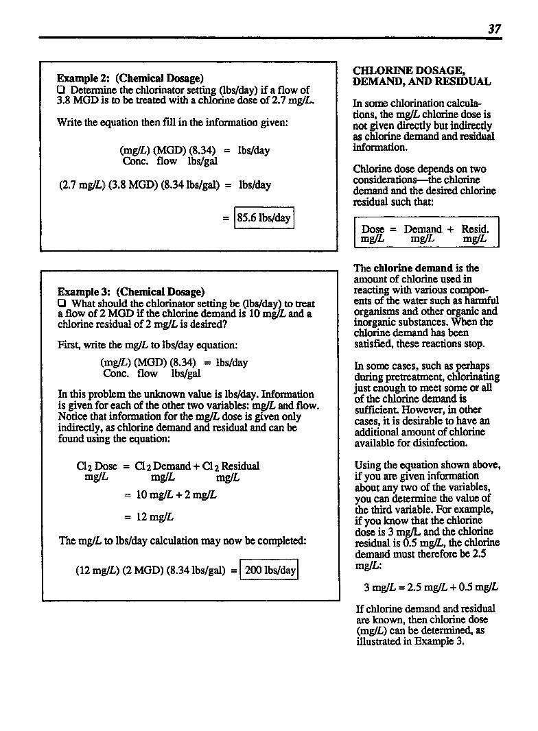
Exampie 2: (Chemical Dosage) P Determine the chlorinator setting (lbslday) if a flow of 3.8 MGD is to be treated with a chlorine dose of 2.7 mglL.
Write the equation then fill in the information given:
(mg/L) (MGD) (8.34) = lbs/day Conc. flow lbs/gal
(2.7 mglL) (3.8 MGD) (8.34 lbslgal) = lbslday
Example 3: (Chemical Dosage) Q What should the chlorinator setting be (lbs/day) to mat a flow of 2 MGD if the chlorine demand is 10 mg/L and a chlorine residual of 2 rngll. is desired?
First, write the m& to lbs/day equation:
(mglL) (MGD) (8.34) = lbslday Conc. flow lbslgal
In this problem the unknown value is lbslday. Information is given for each of the other two variables: mglL and flow. Notice that information for the mglL dose is given only indirectly, as chlorine demand and residual and can be found using the equation:
C1 2 Dose = C1 2 Demand + Cl 2 Residual mglL mgl' mglL
, The mg/L to lbslday calculation may now be completed:
(12 mglL) (2 MGD) (8.34 lbs/gal) = -1
CHLORINE DOSAGE, DEMAND, AND RESIDUAL
In some chlorination calcula- tions, the mglL chlorine dose is not given directly but indirectly as chlorine demand and residual information.
Chlorine dose depends on two considerations-the chlorine demand and the d e s a chlorine residual such that:
Dose = Demand + Resid. m@ I
The chlorine demand is the amount of chlorine used in reacting with various compon- ents of the water such as harmful organisms and other organic and inorganic substances. When the chlorine demand has been satisfied, these reactions stop.
In some cases, such as perhaps during pretreatment, chlorinating just enough to meet some or al l of the chlorine demand is sufficien~ However, in other cases, it is desirable to have an additional amount of chlorine available for disinfection.
Using the equation shown above, if you are given information about any two of the variables, you can determine the value of the third variable. For example, if you know that the chlorine dose is 3 m@ and the chlorine residual is 0.5 mglL, the chlorine demand must therefore be 2.5 mgfL:
If chlorine demand and residual are known, then chlorine dose (mglL) can be determined, as illustrated in Example 3.
38 Chapter 3 MILLIGRAMS PER LITER TO POUNDS PER DAY CALCULATIONS
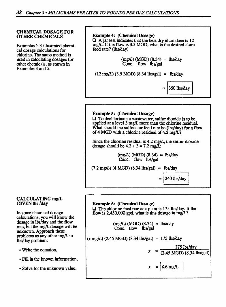
CHEMICAL DOSAGE FOR OTHER CHEMICALS
Examples 1-3 illustrated chemi- cal dosage calculations for chlorine. The same method is used in calculating dosages for other chemicals, as shown in Examples 4 and 5.
CALCULATING mglL GIVEN Ibs /day
In some chemical dosage calculations, you will know the dosage in lbs/day and the flow rate, but the mg/L dosage will be unknown. Approach these problems as any other mg/L to lbslday problem:
Write the equation,
Fill in the known information,
Solve for the unknown value.
Example 4: (Chemical Dosage) Cl A jar test indicates that the best dry alum dose is 12 mg/L. If the flow is 3.5 MGD, what is the desired alum feed rate? (lbs/day)
(mg/L) (MGD) (8.34) = lbs/day Conc. flow lbs/gal
Example 5: (Chemical Dosage) D To dechlorinate a wastewater, s u b dioxide is to be applied at a level 3 mg/L more than the chlorine residual. What should the sulfonator feed rate be (lbs/day) for a flow of 4 MGD with a chlorine residual of 4.2 mglL?
Since the chlorine residual is 4.2 mglL, the s u l k dioxide dosage should be 4.2 + 3 = 7.2 m g l '
(mg/L) (MGD) (8.34) = lbs/day Conc. flow lbs/gal
(7.2 m@) (4 MGD) (8.34 lbs/gal) = lbs/day
Example 6: (Chemical Dosage) P The chlorine feed rate at a plant is 175 lbs/day. If the flow is 2,450,000 gpd, what is this dosage in mglL?
(mg/L) (MGD) (8.34) = lbslday Conc. flow lbslgal
(X mg/L) (2.45 MGD) (8.34 lbslgal) = 175 lbslday
175 lbsldav X ' (2.45 MGD) (8.34 lbslgal)

Chemical Dosage 39
Example 7: (Chemical Dosage) P A stora e tank is to be disinfected with a 50 mglL f chlorine so ution. If the tank holds 70,000 gallons, how many pounds of chlorine (gas) will be needed?
(mg/L) (MG) (8.34) = lbs Conc. Vol Ibs/gal
(50 mg/L) (0.07 MG) (8.34 lbs/gal) = lbs
Example 8: (Chemical Dosage) Q To neutralize a sour digester, one ound of lime is to be added for every pound of volatile aci 8, in the digester liquor. If the digester contains 250,000 gal of sludge with a volatile acid (VA) level of 2,300 mgfL, how many pounds of lime should be added?
Since the VA concentration is 2300 m& the lime concentration should also be 2300 m&:
(mdL) (MG) (8.34) = lbs Conc. Vol lbs/gal
(2300 mglL) (0.25 MG) (8.34 lbs/gal) = lbs
n
CHEMICAL DOSAGE IN WELLS, TANKS, RESERVOIRS, OR PIPELINES
Wells are disinfected (chlor- inated) during and after con- struction and also after any well or pump repairs. Tanks and reservoirs are chlorinated after initial inspection and after any time they have been drained for cleaning, repair or maintenance. Similarly, a pipeline is chlorinated after initial installa- tion and after any repair.
Digesters may also require che- mical dosing, although the che- mical used is not chlorine but lime or some other chemical.
For calculations such as these, use the mglL to lbs equation:
l (m@) (MG) (8.34) = lbs Conc. Vol Ibs/gal 1
Notice that this equation is very similar to that used in Examples 1-6. The only difference is that MG volume is used rather than MGD flow; therefore, the result is lbs rather than lbslday. (When dosing a volume, there is no time factor consideration.) Examples 7-8 illustrau these calculations.

40 Chapter 3 MUGRAMS PER UTER TO POUNDS PER DAY CALCULATIONS
HYPOCHLORITE COMPOUNDS
When chlorinating water or wastewater with chlorine gas, you are chlorinating with 100% available chlorine. Therefore, if the chlorine demand and residual requires 50 lbs/day chlorine, the chlorinator setting would be just that-50 lbsD4 hrs.
Many times, however, a chlorine compound called hypochlorite is used to chlorinate water or was tewater. Hypochlorite com- pounds contain chlorine and are similar to a strong bleach. They are available in liquid form or as powder or granules. Calcium- h ypochlori te, sometimes referred to as HTH is the most com- monly used dry hypochlorite. It contains about 65 % available chlorine. Sodium hypochlorite, or liquid bleach, contains about 12- 15% available chlorine as commercial bleach or 34.25% as household bleach.
Because hypochlorite is not 100% pure chlorine, more Ibdday must be fed into the system to obtain the same amount of chlorine for disinfect ion.
To calculate the lbslday hypo- chlorite required: 1. First calculate the lbslday
chlorine required.
I (mg/~) (MOD) (8.34) = lbs/day 1 Conc. flow lbslgal
2. Then calculate the lbslday hypochlorite needed by dividing the lbslday chlorine by the percent available chlorine.
Chlorine, lbslday - Hypochlorite - % Available lbslday
loo
Example 9: (Chemical Dosage) O A total chlorine dosa e of 12 mg/L is uired to treat a particular water. If the f f ow is l .2 MGD an 7 the hypochlorite has 65% available chlorine how many lbslday of hypochlorite will be required?
First, calculate the lbslday chlorine required using the mg/L to lbslday equation:
(mg/L) (MGD) (8.34) = lbslday Conc. flow lbslgal
(12 mglL) (1.2 MGD) (8.34 lbslgal) = lbslday
= l 120 lbslday 1 Now calculate the lbslday h ypoc hlorite required. Since only 65% of the hypochlorite is chlorine, more than 120 lbs/&y will be required:
1 i
120 lbsby Cl r l 185 lbslday 1 65 Avail. C1 2 - Hy~ochlorite - 100
Example 10: (Chemical Dosage) O A wastewater flow of 850,000 pdires a chlorine dose of 25 mglL. If sodium hypoc orite 15% available chlorine) is to be used, how many lbs/day of sodium hypochlorite are required? How many g a m y of sodium hypochlorite is this?
First, calculate the lbslday chlorine required:
(m@) (MGD) (8.34) = lbslday Conc. flow lbslgal -
(25 m&) (0.85 MGD) (8.34 lbslgal) = lbs/ldy l Chlorine I I I
Then calculate the l bslday sodium h ypochlorite:
177 lbslday C1 2 =I ll8Olbslday I l5 Avail. Cl 2 Hypochlorite
Then calculate the gallday sodium hypochlorite:
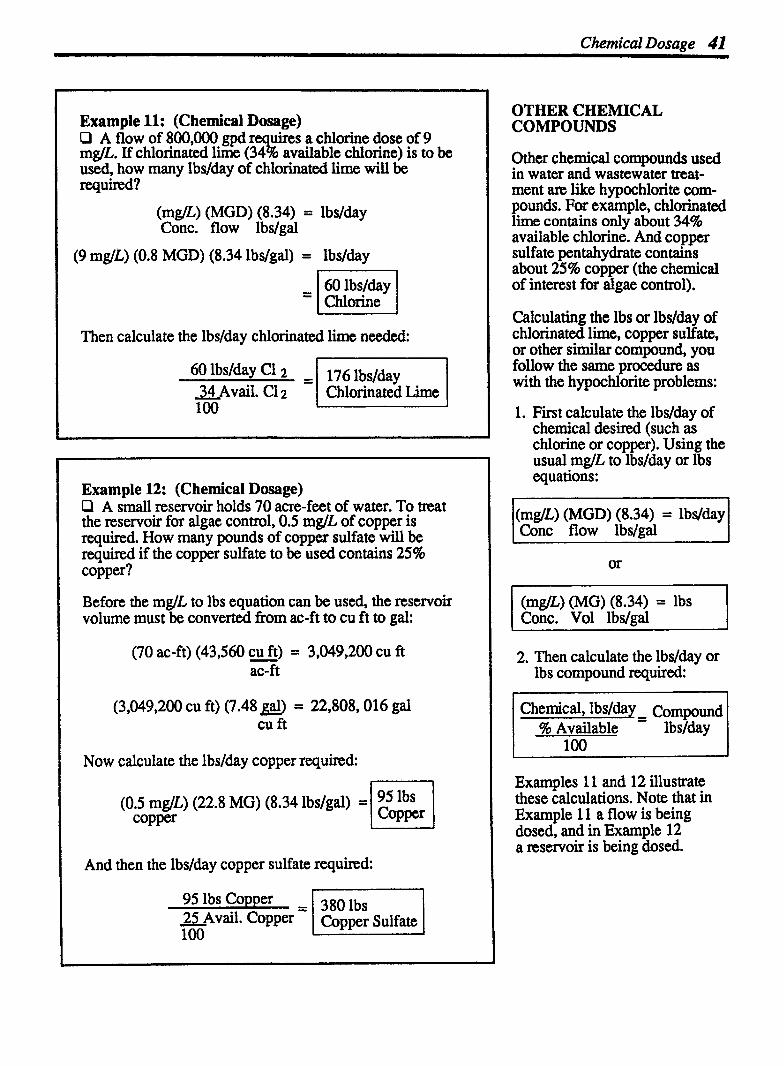
Chemical Dosage 41
Example 11: (Chemical Dosage) 0 A flow of 800,000 gpd uires a chlorine dose of 9 "b mglL. If chlorinated lime (34 o available chlorine) is to be used, how many lbslday of chlorinated lime will be required?
(mglL) (MGD) (8.34) = lbs/day Conc. flow lbslgal
(9 mglL) (0.8 MGD) (8.34 lbslgal) = lbslday - 60 lbslday
= I Chlorine 1 Then calculate the lbslday chlorinated lime needed:
Example 12: (Chemical Dosage) O A small reservoir holds 70 acre-feet of water. To treat the reservoir for algae control, 0.5 mglL of copper is required. How many pounds of copper sulfate will be required if the copper sulfate to be used contains 25% copper?
Before the mglL to lbs equation can be used, the reservoir volume must be converted from ac-ft to cu ft to gal:
(70 ac-ft) (43,560 cu ft) = 3,049,200 cu ft ac- ft
(3,049,200 cu ft) (7.48 galJ = 22,808,016 gal cu ft
Now calculate the lbslday copper required:
(0.5 @L) (22.8 MG) (8.34 lbslgal) = copper
95 lbs
And then the lbslday copper sulfate required:
95 lbs Copper - 25 Avail* Copper 100
OTHER CHEMICAL COMPOUNDS
Other chemical compounds used in water and wastewater treat- ment are like hypochlorite com- pounds. For example, chlorinated lime contains only about 34% available chlorine. And copper sulfate pentahydrate contains about 25% copper (the chemical of interest for algae control).
Calculating the lbs or lbs/&y of chlorinated lime, copper sulfate, or other similar compound, you follow the same procedure as with the hypochlorite problems:
1. First calculate the lbslday of chemical desired (such as chlorine or copper). Using the usual mglL to lbs/day or lbs equations:
l(mg/~) (MGD) (8.34) = lbs/day l Conc flow lbslgal
(mg/L) (MG) (8.34) = lbs Conc. Vol lbslgal
2. Then calculate the lbslday or lbs compound required:
Chemical, lbslday - Compound % Available - lbslday
loo
Examples 11 and 12 illustrate these calculations. Note that in Example 11 a flow is being dosed, and in Example 12 a reservoir is being dosed.
42 Chapter 3 MILLIGRAMS PER LITER TO POUNDS PER DAY CALCULATlONS
3.2 LOADING CALCULATIONS-BOD, COD AND SS
When calculating BOD (Biochemical Oxygen Demand), COD (Chemical Oxygen Demand), or SS (Suspended Solids) loading on a treatment system, the following equation is used:
l (mg/L) (MGD) (8.34) = lbs/day Conc. flow lbs/gal 1 Loading on a system is usually calculated as lbs/day. Given the BOD, COD, or SS concentration and flow information, the lbs/day loading may be calculated as demonstrated in Examples 1-3.
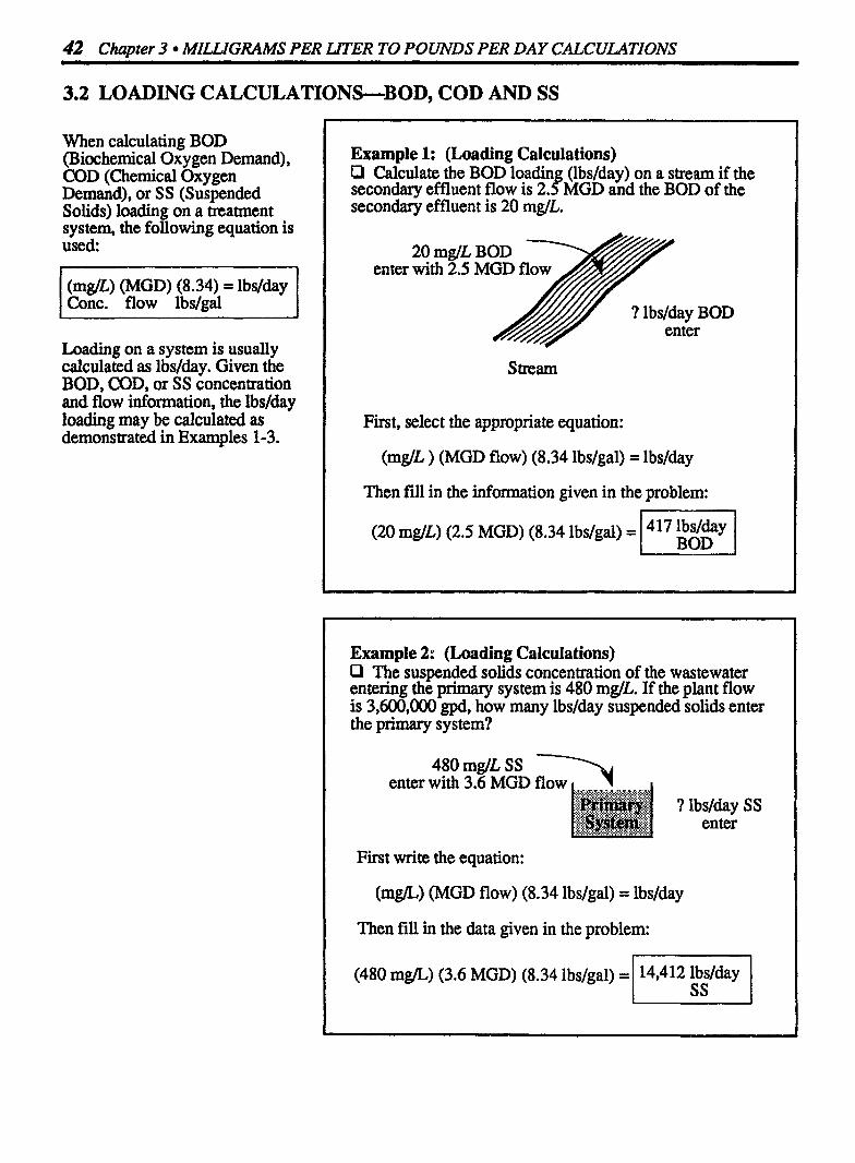
Example 1: (Loading Calculations) P Calculate the BOD loadin (lbslday) on a stream if the secondary effluent flow is 2. !! MGD and the BOD of the secondary effluent is 20 mg/L.
Stream
First, select the appropriate equation:
(mglL ) (MGD flow) (8.34 lbslgal) = lbslday
Then fill in the information given in the problem:
(20 mglL) (2.5 MGD) (8.34 lbs/gal) =
Example 2: (Loading Calculations) P The suspended solids concentration of the wastewater entering the primary system is 480 mglL. If the plant flow is 3,600,000 gpd, how many lbslday suspended solids enter the primary system?
480 m& SS enter with 3.6 MGD
? Ibs/day SS enter
First write the equation:
(m@) (MGD flow) (8.34 lbslgal) = lbslday
Then fill in the data given in the problem:
(480 m&) (3.6 MGD) (8.34 lbslgal) = 14,412 Ibs/day l SS

Loading Calculations 43
Example 3: (Loading Calculations) O The flow to an aeration tank is 7 MGD. If the COD concentration of the water is 110 mglL, how many pounds of COD are applied to the aeration tank daily?
enter l l O m g l L S S y with 7 MGD flow .
Use the mglL to lbs/day equation to solve the problem:
(l l0 mg/L) (7 MGD) (8.34 lbs/gal) = COD
Example 4: (Loading Calculations) Q he daily flow to atrickling filter is 4,500,000 gpd. If the BOD concentration of the trickling fdter influent is 213 rnglL, how many lbs BOD enter h e trickling filter daily?
Write the equation, fill in the given information, then solve for the unknown value:
(mglL) (MGD flow) (8.34 lbs/gal) = lbs/day
(213mglL)(4.5MGD)(8.341bs/gal) 79941bslday 1 BOD I

44 C b t e r 3 MILLIGRAMS PER LlTER TO POUNDS PER DAY CALCULATIONS
3.3 BOD AND SS REMOVAL CALCULATIONS, lbslday
To calculate the pounds of BOD or suspended solids removed each day, you will need to know the mg/L BOD or SS removed and the plant flow. Then you can use the mglL to lbslday equation:
(mg/..) (MGD) (8.34) = lbs/day Removed flow h / g d
For most calculations of BOD or SS removal, you will not be given information stating how many mglL BOD or SS have been removed. This is something you will calculate based on the mglL concentrations entering (influent) and leaving (effluent) the system.
The influent BOD or SS concentration indicates how much BOD or SS is entering the system. The effluent concen- tration indicates how much is still in the wastewater (the part not removed). The mglL SS or BOD removed would therefore be:
I Influent - Effluent = Removed SS mglL SS mglL SS mglL
Once you have determined the mg/L BOD or SS removed, you can then continue with the usual mg/L to lbslday equation to calculate lbs/day BOD or SS removed. Examples 2-4 illustrate this calculation.
Example 1: (BOD and SS Removal) P If 130 mglL suspended solids are removed by a prim
when the flow is 7.4 MGD? z clarifier, how many lbs/day suspended solids are remov
130 mg/L SS Removed
(mglL) (MGD flow) (8.34 lbslgal) = lbslday
(130 mg/L) (7.4 MGD) (8.34 lbslgal) = SS Removed
Example 2: (BOD and SS Removal) P The flow to a trickling filter is 3.7 MGD. If the primary effluent has a BOD concentration of 180 mglL and the trickling filter effluent has a BOD concentration of 28 mg/L, how many pounds of BOD are removed daily?
IS2 mglL SS BOD Removed
After calculating mglL BOD removed, you can now calculate lbs/day BOD removed:
(mglL) (MGD flow) (8.34 lbslgal) = lbslday Removed Removed
(152 mgL) (3.7 MOD) (8.34 lbdgal) = 4690 lbs/&y I BOD Removed

BOD and SS Removal 45
Example 3: (BOD and SS Removal) P The flow to a primary clarifier is 2.7 MGD. If the influent to the clarifier has a suspended solids concentration of 230 mg/L and the primary effluent has 110 mg/L SS, how many lbs/day suspended solids are removed by the clarifier?
Now calculate lbsfday SS remove&
(mg/L) (MGD flow) (8.34 lbslgal) = lbslday
(120 mg/L) (2.7 MGD) (8.34 lbdgal) = SS Removed
Example 4: (BOD and SS Removal) P The flow to a tricklin filter is 4,600,000 gpd, with a f BOD concentration of 1 5 mglL. If theBOD of the trickling filter effluent is 98 mglL, how many lbslday BOD are removed by the trickling fdter ?
Now calculate lbslday BOD removed:
(mdL) (MGD flow) (8.34 lbs/gal) = lbs/day
(97 mglL) (4.6 MGD) (8.34 lbs/gal) = 3721 lbs/day (BOD Removed
46 Choprer 3 MILLIGRAMS PER LITER TO POUNDS PER DAY CALCULATIONS
3.4 POUNDS OF SOLIDS UNDER AERATION CALCULATIONS
In any activated sludge system it is important to control the amount of solids under aeration (solids inventory). The suspended solids in an aerator are called Mixed Liquor Suspended Solids (MLSS). To calculate the pounds of suspended solids in the aeration tank, you will need to know the mglL concentration of the MLSS. Then mglL MLSS can be expressed as lbs MLSS, using the mglL to lbs equation:
(mg/L) (MG) (8.34) = lbs MLSS Vol lbslgal
Notice that the mixed liquor suspended solids concentration is concentration within a tank. Therefore, the equation using MG volume is used.
Another important measure of solids in the aeration tank is the amount of volatile suspended solids. * The volatile solids content of the aeration tank is used as an estimate of the microorganism population of the aeration tank. The Mixed Liquor Volatile Suspended Solids (MLVSS) usually comprises about 70% of the MLSS. The other 30% of the MLSS are fixed (inorganic) solids. To calculate the lbs MLVSS, use the mglL to lbs equation:
(mg/L) (MG) (8.34) = lbs MLVSS Vol lbdgal
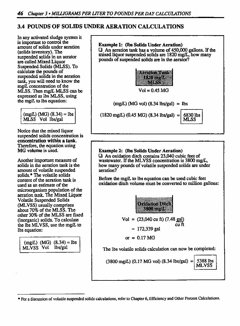
Example 1: (lbs Solids Under Aeration) P An aeration tank has a volume of 450,000 gallons. If the mixed liquor suspended solids are 1820 mg/L, how many pounds of suspended solids an in the aerator?
Vol = 0.45 MG
(mglL) (MG vol) (8.34 lbslgal) = lbs - (1820 mglL) (0.45 MG) (8.34 lbslgal) = 6830 lbs I I
Example 2: (lbs Solids Under Aeration) P An oxidation ditch contains 23,040 cubic fect of wastewater. If the MLVSS concentration is 3800 mglL, how many pounds of volatile suspended solids are under aeration?
Before the mglL to lbs equation can be used cubic fett oxidation ditch volume must be converted to million gallons:
Vol = (23,040 cu ft) (7.48 @ cu ft
= 172,339 gal
The lbs volatile solids calculation can now be completed.
(3800 mglL) (0.17 MG vol) (8.34 lbslgal) = 12% l
* For a discussion of volatile suspended solids calculations, refer to Chapter 6, Efficiency and Other Percent Calculations.

Solids Under Aeration 47
Example 3: (lbs Solids Under Aeration) O The aeration tank of a conventional activated sludge plant has a mixed liquor volatile suspended solids concentration of 2300 m&. If the aeration basin is l l0 ft long, 35 ft wide and has wastewater to a depth of 13 ft, how many pounds of MLVSS are under aeration?
Vol = (110 ft) (35 ft) (13 ft) (7.48 gal)
= 374,374 gal cu ft
Now calculate lbs MLVSS using the usual equation and fill in the given information:
(2300 mglL) (0.37 MG) (8.34 lbs/gal) = 7097 lbs I MLVSS /
Example 4: (lbs Solids Under Aeration) Q An aeration tank is 90 ft lon and 40 ft wide. The de th f of wastewater in the tank is 16 t. If the concentration o F MLSS is 1980 m&, how many pounds of MLSS are under aeration?
Vol = (90 ft) (40 ft) (16 ft) (7.48 g& cu ft
= 430,848 gal
Now N1 in the mg/L to lbs equation with known information:
(1980 mglL) (0.43 MG) (8.34 lbs/gal) = 7101 lbs MLSS r

48 C-er 3 MILLIGRAMS PER LJTER TO POUNDS PER DAY CALCULATIONS
3.5 WAS PUMPING RATE CALCULATIONS
Waste Activated Sludge (WAS) pumping rate calculations are calculations that involve mglL and flow. Therefore the equation used in these calculations is:
(mglL) (MGD) (8.34) = lbs/day I flow lbs/gal
In WAS pumping rate calculations, the "WAS SS" refers to the suspended solids content of the Waste Activated Sludge being pumped away, and "MGD flow" refers to the WAS pumping rate of the sludge being wasted.
Sometimes waste activated sludge SS is not known but return activated sludge SS is known. Remember that RAS SS and WAS SS are the same measurement. It is a measure- ment taken of secondary clarifier sludge. This sludge is either pumped back to the aerator (RAS) or wasted (WAS).
WAS PUMPING RATE CALCULATIONS ARE mglL TO Ibs/day PROBLEMS:
(mglL) (MGD) (8.34) = Ibs/day
f WAS SS Dry Suspended
Solids Pumped Rate, MGD Away
Example 1: (WAS Pumping Rate Calculations) Q The WAS suspended solids concentration is 5860 mglL. If 3800 lbs/day dry solids are to be wasted, (a) What must the WAS pumping rate be, in MGD? (b) What is this rate expressed in gpm?
(a) First calculate the MGD pumping rate required, using the mg/L to lbs/day equation:
(mg/L) (MGD flow) (8.34 lbs/gal) = lbslday
(5860) (xMGD) (8.34) = 38001bs/day mglL flow lbs/day
3800 lbs/day X =
(5600) (8.34) mglL lbdgal
(b) Then convert the MGD flow to gpm flow: *
0.08 l4 MGD = 8 1,400 gpd
= 81,400gpd 1440 midday
* Refer to Chapter 8 in Basic Math Concepts for a review of flow conversions.
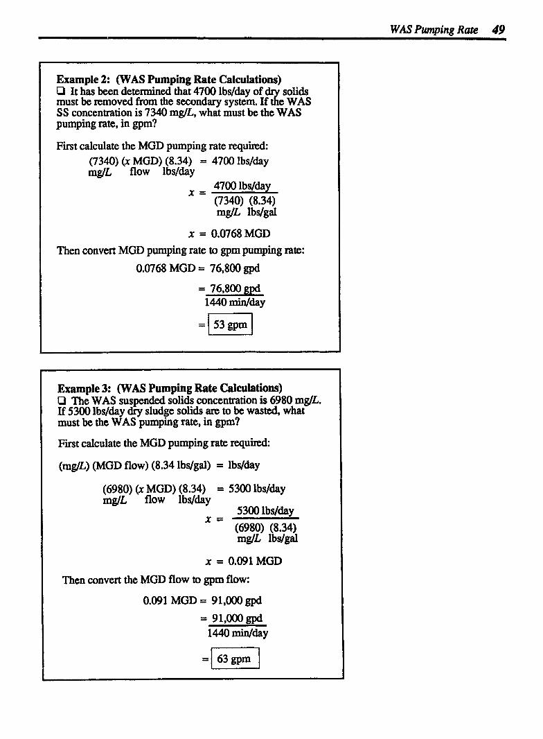
WAS Pumping Rate 49
Example 2: (WAS Pumping Rate Calculations) P It has been determined that 4700 lbs/day of must be removed from the secondary system. If % e WAS SS concentration is 7340 mglL, what must be the WAS pumping rate, in gpm?
First calculate the MGD pumping rate required: (7340) (X MGD) (8.34) = 4700 lbs/day mglL flow lbslday
X = 0.0768 MGD Then convert MGD pumping rate to gpm pumping rate:
0.0768 MGD = 76,800 gpd
Example 3: (WAS Pumping Rate Calculations) 0 The WAS suspended solids concentration is 6980 mgLL. If 5300 lbs/day dry sludge solids are to be wasted, what must be the WAS pumping rate, in gpm?
First calculate the MGD pumping rate required:
(mg/L) (MGD flow) (8.34 lbslgal) = lbs/day
(6980) (X MGD) (8.34) = 5300 lbs/day mg/L flow lbs/day
X = 5300 lbs/day (6980) (8.34) mglL lbs/gal
X = 0.091 MGD
Then convert the MGD flow to gprn flow:
0.091 MGD = 91,000 gpd


4 Loading Rate Calculations
1. The hydraulic loading rate of a treatment system is a measure of the flow treated per square foot of surface area. The most common expression of hydraulic loading rate is gpd/sq ft. Recirculated flows are included as part of the gpd flow to the system.
I Total gpd flow (includes recirc.) 7
Total gpd flow (includes recirc .) -3
sq ft area sq ft area
Hydraulic Loading = Flow, gpd Rate Area, sq ft
Hydraulic loading rate for ponds is generally expressed as inches /day:
acres area
Hydraulic Loading - Flow, ac-ft/day Rate
- Area, ac
Then, multiplying by 12 inJft, the hydraulic loading rate can be expressed in in./day.
Hydraulic Loading - - - in. Rate day
There are several calculations that measure the water and solids loading on the treatment system. When the water and solids loading consistently exceed design values, the efficiency of the treatment system begins to deteriorate.
Calculations that reflect various types of water loading on the system include:
Hydraulic Loading Rate (gpd/sq ft)
Surface Loading Rate (gpdsq ft, gpm/sq ft or in./day)
Filtration Rate (gpm/sq ft or inJmin)
Backwash Rate (gpm/sq ft or in./min)
Unit Filter Run Volume, UFRV, (gavsq ft)
Weir Overflow Rate (gpdlft)
Calculations that reflect various types of solids loading are:
Organic Loading Rate (lbs BOD/day/1000 cu ft)
Food/Microorganism Ratio (lbs BODIdayPb MLVSS)
Solids Loading Rate (lbs SS/day/sq ft)
Digester Loading Rate (lbsVS/day/cu ft)
Digester Volatile Solids Loading Ratio (lbs VSIday Added/lb VS in Digester)
Population Loading and Population Equivalent

52 Chapter 4 LOADING RATE CALCULATIONS
2. Surface overflow rate is a calculation similar to hydraulic loading rate-flow rate per unit area. The difference between these calculations pertains to recirculation rates. Recirculation is not included in the surface overflow rate calculation.
I sq ft area sq ft area
Surface Overflow - mows g ~ d I Rate -
Area, sq ft
I 3. Filtration rate is a measure of the gallons per minute flow filtered by each square foot of filter.
sq ft filter area
Filtration = Flow, gpm 1 Rate Area, sq ft
4. Backwash rate is a very similar calculation to filtration rate. It is the gallons per minute of backwash water flowing through each square foot of filter area.
gpm flow I
sq ft filter area
Flow, gpm Backwash = I Rate Area, sq ft

5. Unit filter run volume (umcV) is a measure of the total gallons of water filtered by each square foot of filter surface area during a filter m.
sq ft filter area
UFRV = Total gal Area, sq ft
6. The weir overflow rate is a measure of the gallons per day flowing over each foot of weir.
ft of weir ft of weir
7. The organic loading rate on a system is the pounds per day of BOD applied to each 1000 cu ft volume.
l b slday BOD 7
U loo0 cu ft volume
I Organic = BOD, lbsfday Loading Volume, 1000 cu ft

54 Chapter 4 LOADING RATE CALCULATIONS
8. The food/microorganimn ratio indicates the relative balance between the food entering the secondary system and the microorganisms pmsent.
I (Microorganism) I/ I v
lbs MLVSS in Aeration Tank
BOD entering, Ibslday MLVSS, lbs
9. Solids loading rate indicates the pounds of solids that are loaded daily per square foot of secondary clarifier surface area.
lbslday solids 7
l clarifier sq ft
Solids Loading - I - Area, sq ft
10. The digester loading rate measures the lbslday volatile solids entering the digester per cubic foot of digester volume.
I cu ft volume
Digester Loading - - VS, lbslday Rate Dig. Volume, cu ft

The digester volatile solids loading ratio is used to determine the seed sludge required in the digester. It can also be used to determine the balance b6tween volatile solids added to the digester and the volatile solid in the digester.
lbslday VS Added '-4
Volatile Solids = VS Added, lbslday Loading Ratio VS in Digester, lbs
Population loading is a calculation most often assbciated with wastewater ponds. It is the number of people served per acre of pond area.
population = People Served by the System Loading Pond Area, acres
Population equivalent is a calculation that expresses the organic content of a wastewater (BOD) in terns of an equivalent number of people using the system. This calculation assumes that for each person using the system, about 0.2 lbslday BOD enter the system.
Population = (mglL BOD) (MGD flow) (8.34 lbslgal) Equivalent 0.2 lbslday BODIperson

56 Chapter 4 LOADING RATE CALCULATIONS
4.1 HYDRAULIC LOADING RATE CALCULATIONS
Hydraulic loading rate is a tern used to indicate the total flow, in gpd, loaded or entering each square foot of water surface area It is the total gpd flow to the process divided by the water surface area of the tank or pond
As shown in the diagram to the right recirculated flows must be included as part of the total flow (total Q) to the process.
HYDRAULIC LOADING RATE INCLUDES RECIRCULATED FLOWS (Trickling Filter Example)
Rimary Effluent Flow
Recirculated Flow v 1
Trickling Filter
L L
Example l: (Hydraulic Loading) Q A trickling filter 80 ft in diameter mats a primary effluent flow of 1.8 MGD. If the recirculated flow is 0.3 MGD, what is the hydraulic loading on the trickling filter?
I Trickling Filter
L-d 0.3 MGD I Hydraulic Loading , How*
Rate Area, sq ft
- - 2,100,000 gpd (0.785) (80 ft) (80 ft)

Hydraulic boding 57
Example 2: (Hydraulic Loading) O If 50,000 gpd are pum ed to a 30 ft diameter gravity thickener, what is the hy aulic loading rate on the thickener?
d:
50,OOO gpd flow 7
Hydraulic Loading - - Flow, gpd Rate Area, sq ft
- - 50,000 ~spd (0.785) (30 Et) (30 ft)
Example 3: (Hydraulic Loading) P A rotating biological contactor treats a flow of 2.8 MGD. The manufacturer's data indicates a media surface area of 80O9000 sq ft. What is the hydraulic loading rate on the RBC?
" ..:.. . ..... " ..:.& ":..
/<&$J&.& +. y:. 3: ,$.:$p:.>,:...:.>.5:.',. ....*... :+:. ..:.:.:?.K.:$+ r: :.
..~$$y~:&yy$$$.<:$~ .~#y$y- ..@B& :'
- - Media Area .2.8 MGD Flow 800,000 sq ft
Hydraulic Loading = Flow, gpd Rate Area, sq ft
- - 2,800,000 gpd 800,000 sq ft
WHEN THERE IS NO RECIRCULATION
When there is no recirculated flow, the total flow applied is simply the flow to the unit process.
HYDRAULIC LOADING FOR ROTATING BIOLOGICAL CONTACTORS (RBC)
When calculating the hydraulic loading rate on a rotating biological contactor, use the sq f't area of the media rather than the sq ft area of the water surface, as in other hydraulic loading calculations. The RBC manufacturer provides media area information.
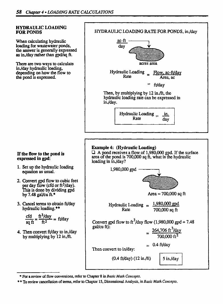
58 Chapter 4 LOADING RATE CALCULATIONS
HYDRAULIC LOADING FOR PONDS
When calculating hydraulic loading for wastewater ponds, the answer is generally expressed as inJday rather than gpd/sq ft.
Thcn are two ways to calculate in./day hydraulic loading, depending on how the flow to the pond is expressed.
If the flow to the pond is expressed in gpd:
1. Set up the hydraulic loading equation as usual.
2. Convert gpd flow to cubic feet per day flow (cfd or ft3/day). This is done by dividing gpd by 7.48 gaVcu ft.*
3. Cancel terms to obtain ftfday hydraulic loading. * *
4. Then convert fr/day to in./day by multiplying by 12 in./ft.
HYDRAULIC LOADING RATE FOR PONDS, inJday
ac-ft V-
acres area
Then, by multiplying by 12 in./ft, the hydraulic loading rate can be expressed in inJday .
Hydraulic Loading = &. 1 I Rate &Y
Example 4: (Hydraulic Loading) Cl A pond receives a flow of 1,980,OOO d. If the surface area of the pond is 700,000 sq ft, what is e hydraulic loading in inJday?
g9,
l ,980,OOO gpd -1
Area = 700,000 sq ft
Hydraulic Loading , 19980,000 md Rate 700,000 sq ft
Convert gpd flow to ft 3/day flow (1,980,OO gpd + 7.48 gucu ft):
= 0.4 ft/day Then convert to in/day:
* For a review of flow conversions, refer to Chapter 8 in Basic Math Concepts. * * To review cancellation of terms, refer to Chapter 15, Dimensional Analysis, in Basic Math Concepts.
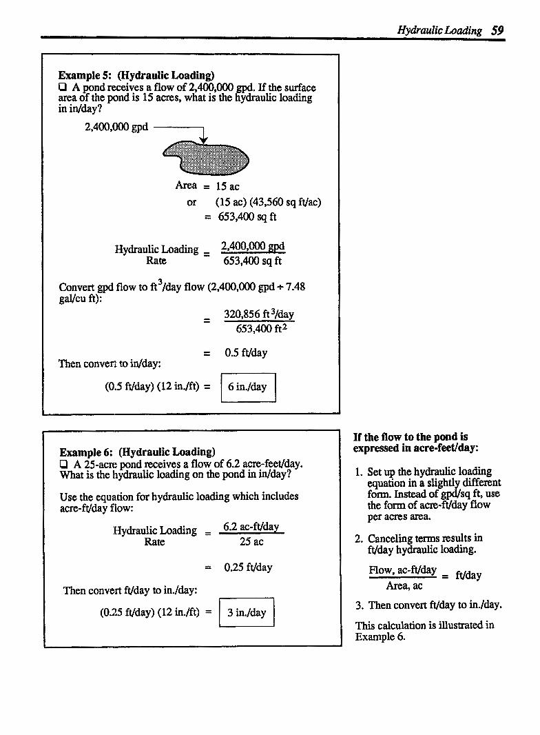
Hydraulic Loading 59
Example 5: (Hydraulic Loading) P A pond receives a flow of 2,400,000 gpd. If the surface area of the pond is 15 acres, what is the hydraulic loading in in/day?
Area = 15 ac or (15ac)(43,560sqft/ac)
= 653,400 sqft
Hydraulic Loading = 2,400,000 gpd Rate 653,400 sq ft
Convert gpd flow to ft '/day flow (2,400,000 gpd + 7.48 gavcu ft):
- - 320,856 ft 3/day 653,400 ft2
= 0.5 ft/day Then convert to idday:
Example 6: (Hydraulic Loading) P A 25-acre pond receives a flow of 6.2 acre-feet/day. What is the hydraulic loading on the pond in infday?
Use the equation for hydraulic loading which includes acre-ft/day flow:
Hydraulic Loading = 602 ac-fvda~ Rate 25 ac
Then convert ft/day to in./day:
(0.25 ftlday) (12 in./ft) = 3 in./day U
If the flow to the pond is expressed in acre-feetlday:
1. Set up the hydraulic loading equation in a slightly different fom. Instead of gpd/sq ft, use the form of acre-ft/day flow per acres area.
2. Canceling terms results in ft/day hydraulic loading.
3. Then convert ft/day to in./day.
This calculation is illustrated in Example 6.

60 Chapter 4 LOADING RATE CALCULATIONS
4.2 SURFACE OVERFLOW RATE CALCULATIONS
Surface overflow rate is used to determine loading on clarifiers. It is similar to hydraulic loading rate-flow per unit area. However, hydraulic loading rate measures the total water entering the pmwss (plant flow plus recirculation) W hereas surface overflow rate measures only the water overflowing the pmess (plant flow only).
As indicated in the diagram to the right, surface overflow rate calculations do not include recirculated flows. This is because recirculated flows are taken from the bottom of the clarifier and hence do not flow up and out of the clarifier (overflow).
Since surface overflow rate is a measure of flow (Q) divided by area (A), surface overflow is an i n h c t measure of the upward velocity of water as it overflows the clflier:*
This calculation is important in maintaining proper clarifier operation since settling solids will be drawn upward and out of the clarifier if surface overflow rates are too high.
Other terms used synonymously with surface overflow rate are:
Surface Loading Rate, and
Surface Settling Rate
SURFACE OVERFLOW RATE DOES NOT INCLUDE RECIRCULATED FLOWS
sq ft area sq ft area
Surface Overflow - - mow, Rate Area, sq ft
Surface overflow rate for wastewater calculations is normally expressed as gpd/sq ft, as shown above. However this calculation for water systems is often expressed as gp* ft.
Surface Overflow = Flow, gprn Rate Area, sq ft
Example 1: (Surface Overflow Rate) P A circular clarifier has a diameter of 60 ft. If the primary effluent flow is 2.3 MGD, what is the surface overflow rate in gpd/sq ft?
(0.785) (60 ft) (60 ft)
Surface Overflow = Flow, gpd Rate Area, sq ft
(0.785) (60 ft) (60 ft)
* Refer to Chapter 2 for a review of Q = AV problems.

Swface Overflow Rate 61
Example 2: (Surface Overflow Rate) O A sedimentation basin 75 ft by 20 ft receives a flow of 1.3 MGD. What is the surface overflow rate in gpd/sq ft?
(75 ft) (20 ft)
Surface Overflow = Flow, gpd Rate Area, sq ft
- 1,300,0(-) gpd (75 ft) (20 ft)
Example 3: (Surface Overflow Rate) P The flow to a sedimentation tank is 3.2 MGD. If the length of the basin is 90 ft and the width is 45 ft, what is the surface overflow rate in gpd/sq ft?
(90 ft) (45 ft)
Surface Overflow = Flow, gpd Rate Area, sq ft
- 3,200,000 gpd (90 ft) (45 ft)

62 Chapter 4 LOADING RATE CALCULATIONS
4.3 FILTRATION RATE CALCULATIONS
The calculation of filtration rate or filter loading rate is similar to that of hydraulic loading rate. It is gprn filtered by each square foot of filter area.
Filtration mow, gPm I Rate -
Area, sq ft
Example l: (Filtration Rate) P A filter 20 ft by 25 ft receives a flow of 1940 gpm. What is the filtra~on rate in gpnJsq ft?
1940 gpm 7
(20 ft) (25 ft)
Filtration gpm Rate Area, sq ft
- - 1940 gpm
(20 ft) (25 ft)
Example 2: (Filtration Rate) O A filter 20 ft by 35 ft treats a flow of 1530 gpm. What is the filtration rate m gpm/sq ft?
1530 gpm ,-l
Filtration Rate
(20 ft) (35 ft)
- - Flow, gpm Area, sq ft
- - 1530 gprn
(20 ft) (35 ft)
Filtration Rate 63
Example 3: (Filtration Rate) Q A filter 25 ft by 30 ft treats a flow of 3.3 MGD. What is the filtration rate m gpmlsq ft?
3,300,000 gpd 1440 min/day = 2292 gprn
Filtration Rate
(20 ft) (35 ft)
- - Flow, gpm Area, sq ft
- 2292 gprn
(25 ft) (30 ft)
Example 4: (Filtration Rate) P A filter has a surface area of 35 ft by 25 ft. If the filter receives a flow of 2,912,000 gpd, what is the fdtration rate in gpm/sq ft?
2,912,000 gpd 1440 minlday
= 2022 gprn
Filtration Rate
(35 ft) (25 ft)
- - How, gprn Area, sq ft
- - 2022 gprn (35 ft) (25 ft)
64 Chapter 4 LOADING RATE CALCULATIONS
4.4 BACKWASH RATE CALCULATIONS
A filter backwash rate is a measurc of the gprn flowing upward through each sq ft of filter surface area The calculation of backwash rate is similar to filtration rate.
Backwash = mow, gpm Rate Area, sq ft
Example 1: (Backwash Rate) D A filter with a surface area of 150 sq ft has a backwash flow rate of 2900 gpm. What is the filter backwash rate in
(10 ft) (15 ft)
Backwash = Rate
Flow, gpm
Ana, sq ft
2900 gpm 150 sq ft
Example 2: (Backwash Rate) O A filter 25 ft by 10 ft has a backwash rate of 3400 gpm. What is the backwash rate in gpdsq ft?
(25 ft) (10 ft)
Backwash = Flow, gpm
Rate Area, sq ft
- - 3400 gpm
(25 ft) (10 ft)

Example 3: (Backwash Rate) O A filter 15 ft by 15 ft has a backwash flow rate of 3150 gpm. What is the filter backwash rate in gpm/sq ft?
(15 ft) (15 ft)
Flow, gprn Backwash = Rate Area, sq ft
- 3150 gprn (15 ft) (15 ft)
Example 4: (Backwash Rate) O A filter 20 ft lon and 15 ft wide has a backwash flow rate of 4.64 MGD. at is the filter backwash rate in gpdsq ft?
&h
(20 ft) (15 ft)
Backwash = Flow, gprn Rate Area, sq ft
- 3222 g j m (20 ft) (15 ft)
WHEN THE FLOW RATE IS EXPRESSED AS GPD
Normally the backwash flow rate is expressed as gpm. If it is expressed in any other flow rate terms, simply convert the given flow rate to gpm.* For example, if gpd flow rate is given, convert the gpd flow rate as follows:
* For a review of flow rate conversions, refer to Chapter 8 in Basic Math Concepts.
66 Chapter 4 LOADING RATE CALCULATIONS
4.5 UNIT FILTER RUN VOLUME CALCULATIONS
The unit filter run volume (UFRV) calculation indicates the total gallons passing through each square foot of filer surface area during an entire filter run. The equation to be used in these calculations is shown to the right
As the performance of the filter begins to deteriorate, the UFRV value will begin to decline as well.
UNIT FILTER RUN VOLUME
Total gallons during filter run
(between backwashes
sq ft Area
Total gal filtered = Filter Area, sq ft
Example 1: (UFRV) O The total water filtered during a filter run (between backwashes) is 2,950,000 gal. If the filter is 15 ft by 20 ft, what is the unit filter run volume (UFRV')?
2,950,000 gal -3
(15 ft) (20 ft)
UFRV = Total gal filtered Filter Area, sq ft
- 2,950,000 gal - (15ft)(20ft)

UFRV 67
Example 2: (UFRV) P The total water filtered during a filter run is 3,220,000. If the filter is 20 ft by 20 ft what is the UFRV?
3,220,000 gal -3
(20 ft) (20 ft)
UFRV = Total gal filtered Filter Area, sq ft
- 3,220,000 gal - (20 ft) (20 ft)
Example 3: (UFRV) 0 The total water filtered during a filter run is 4,583,0001 If the filter is 20 ft by 30 ft, what is the unit filter run volume?
4,583,000 gal -3
(20 ft) (30 ft)
Total gal filtered = Filter Area, sq ft
- - 4,583,000 gal (20 ft) (30 ft)

68 Chapter 4 LOADING RATE CALCULATIONS
4.6 WEIR OVERFLOW RATE CALCULATIONS
Weir overflow rate is a measure of the gallons per day flowing over each foot of weir.
Weir Overflow, Flow, Rate Weir Length, ft
CALCULATING WEIR CIRCUMFERENCE
In some calculations of weir ovefflow rate, you will have to calculate the total weir length given the weir diameter. To calculate the length of weir around the clarifier, you need to know the relationship between the diameter and circumference of a circle. The distance around any circle (circumference) is about three times the distance across the circle (diameter). In fact, the circumference is (3.14) (Diameter).* Therefore, given a diameter, the total ft of weir can be calculated as:
Weir Length, = (3.14) (Weir Diam. ,)
ft ft
Example 1: (Weir Overflow Rate) O A rectangular clarifier has a total of 100 ft of weir. What is the weir overflow rate in gpd/ft when the flow is 1.2 MGD?
100 ft weir
Weir Overflow , Flow, gpd Rate - Weir Length, ft
Example 2: (Weir Overflow Rate) D A circular clarifier receives a flow of 3.38 MGD. If the diameter of the weir is 80 ft, what is the weir overflow rate in gpd/ft?
The total ft of weir is not given directly in this problem. However, weir diameter is given (80 ft) and from that information we can determine the length of the weir.
ft weir: = (3.14) (80 ft) = 251 ft
Weir Overflow = Flow, gpd Rate Weir Length, ft
- - 3,380,000 gpd
251 ft
* For a review of circumference calculations, refer to Chapter 9, Linear Measurement, in Basic Math Concepts..

Weir O v e M w Rate 69
Example 3: (Weir Overflow Rate) O The flow to a circular clarifier is 2.12 MGD. If the diameter of the weir is 60 ft, what is the weir overflow rate in gpd/ft?
ft weir: = (3.14) (60 ft) = 188 ft
Weir Overflow = Flow, gpd Rate Weir Length, ft
Example 4: (Weir Overflow Rate) Q A rectangular sedimentation basin has a total weir length of 80 ft. If the flow to the basin is 1.3 MGD, what is the weir loading rate in gpdft?
Weir Loading - Flow, gpm Rate Weir Length, ft
- - 903 gprn 80 ft weir
WEIR LOADING RATE
Weir overflow rate is a term most often associated with was tewater clarifier calculations. A similar calculation often used for water system clarifiers is weir loading rate, expressed as gpm/ft.

70 Chapter 4 LOADING RATE CALCULATIONS
4.7 ORGANIC LOADING RATE CALCULATIONS
When calculating the pounds of BOD entering a wastewater process daily, you are calculating the organic load on the process-the food entering that process. Organic loading for trickling fdters is calculated as lbs BODlday per 1000 cu ft media:
Organic Loading - - BODY lbslday I Rate Vol., loo0 cu ft I I In most instances BOD will be expressed as a m& concen- tration and must be converted to lbs BOD/day.* Therefore the equation given above can be expanded as:
(m& BOD) (MOD) (8.34) O.L., flow ibs/gal l (
Note that the "1000" in the denominator of both equations is a unit of measure ("thousand cu ft") and is not part of the numerical calculation.
To determine the number of 1000 cu ft, find the thousands comma and place a decimal at that position. In Example 1, 19,233 cu ft is 19.233 units of 1000 cu ft. So 19.233 is placed in the denominator.
Example l: (Organic Loading Rate) P A trickling Nter 70 ft in diameter with a media depth of 5 feet receives a flow of 1,150,000 gpd. If the BOD concentration of the primary effluent is 230 mglL, what is the organic loading on the trickling filter?
BOD, lbslda \L
U (0.785) (70 ft) (70 ft) (5 ft) = 19,233 cu ft
Organic Loading = BOD, Ibslday Rate Volume, 1OO0 cu ft
- - (230 mglL) (1.15 MGD) (8.34 lbslgal)
Example 2: (Organic Loading Rate) P A100-ft diameter trickling fdter with a media depth of 4 ft receives a primary effluent flow of 1.65 MGD with a BOD of 105 mg/L. What is the organic loading on the trickling fdter?
BOD, lbslday ---
U (0.785) (100 ft) (100 ft) (4 ft) = 31,400 cu ft
- - (105 mg/L) (1.65 MGD) (8.34 lbs/gal) 31.4 1000-cu ft
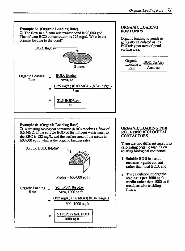
O r m i c Loading Rate 71
Example 3: (Organic Loading Rate) Cl The flow to a 3-acre wastewater pond is 90,000 gpd. The influent BOD concentration is 125 mglL. What is the organic loading to the pond?
BOD, lbslday-J,
3 acres
Organic Loading BOD, lbslday Rate Area, ac
- - (125 mg/L) (0.09 MGD) (8.34 lbslgal) 3 ac
Example 4: (Organic Loading Rate) D A rotatin biolo 'cal contactor (RBC) receives a flow of 3.6 MGD. &he sogble BOD of the influent wastewater to the RBC is 122 mg/L, and the surface area of the media is 600,000 sq ft, what is the organic loading rate?
Soluble BOD, lbslday ,-\
Media = 600,000 sq ft
Organic Loading = Sol. BOD, lbs /day Rate Area, 1OOO sq ft
- - (122 mg/L) (3.6 MGD) (8.34 lbslgal) 600 1000-sq ft
= 1 6.1 lbslday Sol. BOD loo0 sq ft
ORGANIC LOADING FOR PONDS
Organic loading to ponds is generally calculated as ibs BODIday per a m of pond surface area.
Orga"'c BOD, lbs/day I Loading =
ORGANIC LOADING FOR ROTATING BIOLOGICAL CONTACTORS
There are two different aspects to calculating organic loading on rotating biological contactors:
1. Soluble BOD is used to measure organic content rather than total BOD, and
2. The calculation of organic loading is per 1000 sq ft media rather than 1000 cu ft media as with trickling filters.
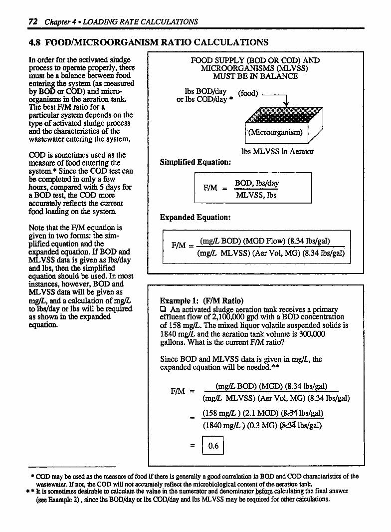
72 Chapter 4 LOADING RATE CALCULATIONS
4.8 FOOD/MICROORGANISM RATIO CALCULATIONS
In order for the activated sludge process to operate properly, there must be a balance between food entering the system (as measured by BOD or COD) and micro- organisms in the aeration tank. The best F/M ratio for a particular system depends on the type of activated sludge process and the characteristics of the wastewater entering the system.
COD is sometimes used as the measure of food entering the system.* Since the COD test can be completed in only a few hours, compared with 5 days for a BOD test, the COD more accurately reflects the current food loading on the system.
Note that the F/M equation is given in two forms: the sim- plified equation and the expanded equation. If BOD and MLVSS data is given as lbslday and lbs? then the simplified equation should be used. In most instances, however, BOD and MLVSS data will be given as mglL, and a calculation of mglL to lbs/day or Ibs will be required as shown in the expanded equation.
FOOD SUPPLY (BOD OR COD) AND MICROORGANISMS (MLVSS)
MUST BE IN BALANCE
lbs BODIday (food) or lbs COD/day *
/ (Microorganism) l/ lbs MLVSS in Aerator
Simplified Equation:
F/M = BOD, lbslday MLVSS, lbs
Expanded Equation:
F/M = (m&L BOD) (MGD Flow) (8.34 lbslgal) (mg/L MLVSS) (Aer Vol, MG) (8.34 lbs/gal)
Example 1: (FIM Ratio) P An activated slud e aeration tank receives a primary effluent flow of 2,l 08 ,000 gpd with a BOD concentra~on of 158 mgIL. The mixed liquor volatile suspended solids is 1840 mglL and the aeration tank volume is 300,000 gallons. What is the current F/M ratio?
Since BOD and MLVSS data is given in m@, the expanded equation will be needed.**
F/M = (m@L BOD) (MGD) (8.34 lbslgal)
(mglL MLVSS) (Aer Vol, MG) (8.34 lbslgal)
- (158 m@ ) (2.1 MGD) (Wf lbslgal) (1 840 mglL ) (0.3 MG) lbslgal)
* COD may be used as the measure of food if there is generally a good correlation in BOD and COD characteristics of the wastewater. If not, the COD will not accurately reflect the microbiological content of the aeration tank. * * It is sometimes desirable to calculate the value in the numerator and denominator before calculating the final answer (see Example 2) . since lbs BODJday or lbs CODJday and lbs MLVSS may be required for other calculations.

Example 2: (FM Ratio) P The volume of an aeration tank is 200,000 gallons. The aeration tank receives a primary effluent flow of 2,320,000 gpd, with a COD concentration of 100 mglL. If the mixed liquor volatile suspended solids is 1900 mglL, what is the current F/M ratio?
Since COD and MLVSS information is given as mglL, the expanded form of the equation is used in the calculation:
F/M = (mg/L COD) (MGD flow) (8.34 lbslgal)
(lbs MLVSS) (Aer Vol, MG) (8.34 lbslgal)
- (1 00 mg/L ) (2.32 MGD) (8.34 lbslgal) (1900 mglL ) (0.2 MGD) (8.34 lbslgal)
(1935 lbs COD/day) -
(3 l69 lbs MLVSS)
Example 3: (FIM Ratio) P The desired F/M ratio at a particular activated sludge plant is 0.5 lbs BOD/1 lb mixed liquor volatile suspended solids. If the 3 MGD primary effluent flow has a BOD of 165 mglL how many lbs of MLVSS should be maintained in the aeration tank?
BOD, lbslday F/M =
MLVSS, lbs
Fill in the equation with the information known. Since BOD is given as mglL, the lbslday BOD must be written in expanded form.
0.5 = (165 m@ ) (3 MGD) (8.34 lbslgal) x lbs MLVSS
Then solve for the unknown value:*
P 1 8257 lbs MLVSS 1
CALCULATING MLVSS USING THE F M RATIO
The F/M ratio calculation can be used to calculate the desired pounds of MLVSS to be maintained in the aerator. Use the same F/M equation, fill in the given information, then solve for the unknown value (MLVSS).*
* To review solving for the unknown value, refer to Chapter 2 in Basic Math Concepts.

74 Chapter 4 4 LOADING RATE CALCULATIONS
4.9 SOLIDS LOADING RATE CALCULATIONS
The solids loading rate indicates the lbslday solids loaded to each square foot of clarifier surface area. This calculation is used to determine solids loading on activated sludge secondary clarifiers and gravity sludge thickeners. The general solids loading rate equation is:
"lids Solids Applied, lbs/day Loading = Rate Surface Area, sq ft
In expanded form, the equation includes the mglL to lbslday calculation in the numeratoe and surface area calculation in the denominator: **
(MLSS ) (MGD) (8.34) - mg/L flow S.L.R. - (0.785) (02)
The vast majority of solids coming into the secondary clarifier comes in as mixed liquor suspended solids (MLSS) from the aeration tank. A negligible amount of suspended solids enter the clarifier by the primary effluent flow. (Remember, up to 70% of the suspended solids are removed by the primary system.)
MOST OF THE SOLIDS LOADED TO THE SECONDARY CLARIFIER ENTER AS MLSS
P.E. Flow
7 I
I I RAS Flow I I I I L,,,,,,,,,,-,,J
MLSS enter the clarifier flow from the aeration tank (Primary Effluent Flow + Return Activated Sludge Flow)
Example 1: (Solids Loading Rate) Q A secondary clarifier is 90 ft in diameter and receives a combined primary effluent (P.E.) and return activated sludge (RAS) flow of 4.9 MGD. If the MLSS concentration in the aeration tank is 3100 mglL, what is the solids loading rate on the secondary clarifier in lbs/&y/sq ft?
Solids, lbs/day ,-l
Solids Loading Rate,
lbslday/sq ft
sq ft Area
(MLSS mg/L) (MGD Flow) (8.34 lbs/gal)
- - (3 100 mg/L) (4.9 MGD) (8.34 lbslgal) (0.785) (90 ft) (90 ft)
= 1 19.9 lbs solidslday 1
* For a review of mg/L to lbs/day calculations refer to Chapter 3. * * Secondary clarifiers are typically circular. For a rectangular clarifier, the surface area would be (l) (W). Area calculations are
discussed in Chapter 10 of Basic Math Concepts.

Solids Loading Rate 75
Example 2: (Solids Loading Rate) O A secondary clarifier 80 ft in diameter receives a primary effluent flow of 3.15 MGD and a return sludge flow of 0.8 MGD. If the MLSS concentration is 3650 mglL, what is the solids loading rate on the clarifier in lbs/day/sq ft?
Solids, lbsjday --J
sq ft Area
Solids L oading Solids, lbsfday Rate, - -
lbs/day/sq ft Area, sq ft
- - (3650 mglL) (3.95 MGD) (8.34 lbslgal) (0.785) (80 ft) (80 ft)
- - 23.9 lbs solidslday sq ft
Example 3: (Solids Loading Rate) O The total flow to a 70-ft diameter clarifier is 4,600,000 gpd (P.E. + RAS flows). If the MLSS concentration is 2500 mglL, what is the solids loading rate on the clarifier in lbsldaylsq ft?
Solids, lbslday -L
sq ft Area
- - Rate, lbslday/sq ft Area, sq ft
- - (2500 mglL) (4.6 MGD) (8.34 lbslgal) (0.785) (70 ft) (70 ft)
24.9 lbs solids/day l

76 Chapter 4 WADING RATE CALCULATIONS
4.10 DIGESTER LOADING RATE CALCULATIONS
Sludge is sent to a digester in order to break down or stabilize the organic portion of the sludge. Therefm, it is the organic part of the sludge (the volatile solids portion) that is of interest when calculating solids loading on a digester.
Digester loading rate is a measure of the pounds of volatile solids* entering each cubic foot of digester volume daily, as illustrated in the diagram to the right.
DIGESTER LOADING
VS Added, lbs/day 7
Digester
cu ft Volume Simplified Equation:
Digester Loading, = VS Added, lbs/day
lbs VS/day/cu ft Volume, cu ft
Expanded Equation:
Digester (Sludge, lbs/day) (% Solids) (% VS)
Loading, = 100 100 lbs VS/day/cu ft (0.785) (D~) (Water Depth, ft)
Example 1: (Digester Loading) P A digester 40 ft in diameter with an operating depth of 20 ft receives 92,700 lbs/day raw sludge. If the sludge contains 6% solids with 69% volatile matter, what is the digester loading in lbs VS added/day/cu ft volume?
VS Added, lbs/day 7
cu ft volume U Digester (Sludge, lbs/day) (% Solids) (% VS) Loading, = 100 100
Ibs VS/&$CU ft (0.785) ( D ~ ) (Water Depth, ft)
- - -
(0.7 85) (40 ft) (40 ft) (20 ft)
* For a review of calculating percent solids and percent volatile solids, refer to Chapter 6.

Digester bading 77
Example 2: (Digester Loading) P A digester 40 ft in diameter operatin at a depth of 18 ft receives 180,000 lbslday sludge with 5 f o total solids and 72% volatile solids. What is the digester loading in lbs VS/day/cu ft?
Digester (Sludge, lbslday) (% Solids) (% VS)
Loading, = 100 100 lbs VSIdaylcu ft (0.785) (D?) (Water Deptli, ft)
(1 80,000 lbslday) (0.05) (0.72) -
(0.785) (40 ft) (40 ft) (18 ft)
= 1 0.29 lbs VSIday I cu ft
Example 3: (Digester Loading) Q A digester 50 ft in diameter operating at a de th of 20 ft B receives 34,300 gpd sludge with 5.5% solids an 70% volatile solids. What is the digester loading in lbs VSldaylcu ft? (Assume the sludge weighs 8.34 lbslgal.)
VS Added, lbslday
cu ft volume U (Sludge, gpd) (8.34 1bsIga.l) (% Sol.) (% VS)
Digester - d. 100 100 - v - Loading, = lbs VS/day/cu ft (0.785) (02) (Water Depth, ft)
9 g (34,300 gpd) (8.34 lbslgal) (0.055) (0.70) (0.785) (50 ft) (50 ft) (20 ft)
= 1 0.28 lbs VSIday cu ft l
GIVEN GPD OR GPM SLUDGE PUMPED TO DIGESTER
In Examples 1 and 2, the sludge pumped to the digester was expressed as lbslday. Many times, however, sludge pumped to the digester is expnssed as gpd or gpm. When this is the case, convert the gpd or gpm pumping rate to lbslday* and continue as in Examples 1 and 2. You can make the gpd to lbslday conversion a separate calculation, or you can incorporate it into the numerator of the equation as shown in Example 3.
* To review flow conversions, refer to Chapter 8 in Baric Math Concepts..

78 Chapter 4 LOADING RATE CALCULATZONS
4.11 DIGESTER VOLATILE SOLIDS LOADING RATIO CALCULATIONS
One way of expressing digester loading was described in the previous section-lbs/&y volatile solids added per cu ft digester volume.
Another way to express digester loading is lbs/&y volatile solids* added per lb of volatile solids under digestion (in the digester).
VOLATILE SOLIDS LOADING RATIO COMPARES VS ADDED WITH VS IN THE DIGESTER
VS Added, lbs/day 7 Digester lbs VS
Simplified Equation:
VS Loading = vs Added, lbdday Ratio VS in Digester, lbs
Expanded Equation: **
VS Loading - - (Sludge Added, lbs/day) (% - Sol) (46 VS) Ratio 100 100
(Sludge in Dig., lbs) (% Sol) (% VS) 100 100
Example 1: (Volatile Solids Loading Ratio) Cl A total of 52,500 lbslday slud e is pumped to a 100,000-gallon digester. The slu f ge being pumped to the digester has total solids content of 5% and volatile solids content of 74%. The sludge in the digester has a solids content of 6% with a 58% volatile solids content. What is the volatile solids loading on the digester in lbs VS added/day/lb VS in digester?
VS Loading VS Added, lbs/&y Ratio VS in Digester, lbs
(52,500 lbs/day) ( 5 ) ( 74 )
- 100 loo (100,OOO gal) (8.34 lbs/gal) ( 6 ) ( 58 )
loo 100 This is lbs digester sludge
* For a review of calculating percent solids and percent volatile solids, refeb to Chapter 6. ** The two hundreds in the numerator and denominator cancel each other out and may be omitted, if desired.
= 0.067 lbs/day VS Added
lb VS in Digester

Digester VS Loading Rario 79
Example 2: (Volatile Solids Loading Ratio) P A total of 22,850 slud e is pumped to an 80,000-gal digester. This sludge p as a so F ids content of 6% and a volatile solids concentration of 72%. The sludge in the digester has a solids content of 5.1 % with a 56% volatile solids content.What is the volatile solids loading on the digester in lbs VS addedfdayflb VS in digester?
VS Loading - - VS Added, lbs/day Ratio VS in Digester, lbs
[ (80,000 gal) (8.34 lbs/gal) ( 5.1 ) (56)
100 100 This is ibs digester sludge
= l 0.052 lbs/day VS Added lb VS in Digester
Example 3: (Volatile Solids Loading Ratio) Q A total of 63,000 sludge is pumped to the digester. pEd The sludge has 4% so ds with a volatile solids content of 74%. If the desired VS loading ratio is 0.08 lbs VS added/lb VS in digester, how many lbs VS should be in the digester for this volatile solids load?
VS Loading VS Added, lbsjday Ratio VS in Digester, lbs
This is ibslday sludge added I
0.08 = (63,000 gpd) (8.34 lbs/day) (4) (74) 100 100
x lbs VS in Digester
Then solve for X:
(63,000) (8.34) (0.04) (0.74)
X = 1 194,405 lbr VS in Digester
CALCULATING OTHER UNKNOWN VALUES
Volatile solids loading ratio calculations have three variables: VS loading ratio, lbs VS addeaday, and lbs VS in the digester.
Given a desired volatile solids loading ratio, you can calculate the desired lbs of volatile solids in the digester. This type of calculation is used for determining seed sludge requirements for startup of a digester. Example 3 illustrates this calculation.

80 Chapter 4 LOADING RATE CALCULATIONS
4.12 POPULATION LOADING AND POPULATION EQUIVALENT
POPULATION LOADING
Population loading is a calcu- lation associated with wastewater treatment by ponds. Populatio~ loading is an indirect measure of both water and solids loading to a system. It is calculated as the number of persons served per acre of pond:
Example 1: (Population Loading) P A 3.5 acre wastewater pond serves a population of 1500. What is the population loading on the pond?
= 1500 persons -
3.5 acres
= l 429 persons acre
Example 2: (Population Loading) P A wastewater pond serves a po ulation of 4OOO. If the pond is l6 acres, what is the pop ation loading on the pond?
Id'
Population - persons Loading acre
- 4000 persons 16 acres

Population Equivalent 81
Example 3: (Population Equivalent) 0 A 0.4-MGD wastewater flow has a BOD concentration of 1800 mglL BOD. Using an average of 0.2 lbslday BOD/person, what is the population equivalent of this wastewater flow?
Population BOD, lbslday lb S BOD/day/person
Convert mg/L BOD to lbs/day BOD* then divide by 0.2 lbs BODIdaylperson:
Population - (1 800 mgL) (0.4 MGD) (8.34 lbslgal) Equivalent - 0.2 lbs BOD/day/person
= ( 30,024 people I
Example 4: (Population Equivalent) P A 100,000 gpd wastewater flow has a BOD content of 2800 m@L. Using an average of 0.2 lbslday BODIperson, what is the population equivalent of this flow?
Population - - BOD, lbslday Equivalent lbs BOD/day/person
- - (2800 mg/L) (0.1 MGD) (8.34 lbslgal) 0.2 lbs BOD/day/person
POPULATION EQUIVALENT
Industrial or commercial waste- water generally has a higher organic content than domestic was tewater. Population equi- valtnt calculations equate these concentrated flows with the number of people that would produce a domestic wastewater of that strength. For a domestic wastewater system, each person served by the system contributes about 0.17 or 0.2 lbs BOD/day . To determine the population equivalent of a wastewater flow, divide the lbs BODIday content by the lbs BOD/day contributed per person (e.g. 0.2 lbs BODIday).
* For a nview of mglL to lbs/day calculations, refer to Chapter 3.


5 Detention and Retention Times Calculations
1. Detention time indicates the amount of time a given flow of water is retained by a unit process. It is calculated as the tank volume divided by the flow rate:
Flow through the tank
Detention Time = Volume of Tank, gal
Flow, gal/time
2. Sludge age is a measure of the average time a sus~ended solids article remains under aeration. sl;dge age (somehmes called Gould sludge age) is based on the pounds of solids added daily to the activated sludge process.
lbslday SS Added 7
Aeration Tank 7 lbs MLSS in Aeration Tank
Simplified Equation:
SS Added, lbslday
Expanded Equation:
Sludge Age = (MLSS mglL) (Aer. Vol., MG) (8.34 lbs/gal) days (P. E. S S, mgL) (Flow, MGD) (8.34 lbs/gal)
In the previous chapter we focused on calculations that measure the water and solids loading on a system. Now we will examine calculations that measure how long the water and solids are retained in the system. Three calculations will be discussed:
Detention Time or Fill Time
Sludge Age
Solids Retention Time (SRT) (also called Mean Cell Residence Time, MCRT)

84 Chapter 5 DETENTON AND RETENTION TIMES
3. Solids Retention Time, SRT (also called Mean Cell Residence Time, MCRT) is another measure of the length of time a suspended solid particle remains under aeration. However, the SRT calculation is based on the pounds of solids leaving the activated sludge process rather than the pounds of solids added, as with sludge age.
RAS Flow
(SS leaving)
Simplified Equation:
Solids Rekntion - Suspended Solids in System, lbs** - Time Suspended Solids Leaving System, lbs/&y
Solids Retention m - Suspended Solids in System lbs** Time WAS SS, lbslday + S.E.* SS, lbdday
Expanded Equation:
SRT, = (MLSS mglL) (Aer. Vol. + Fin. Clar. Vol., MG) (8.34 lbslgal) days (WAS SS) ( WAS Flow) (8.34) + (S.E. SS) (Plant Flow) (8.34)
W& MGD lbslgal mglL MGD lbs/gd
* S.E. is an abbreviation for Secondary Effluent. P.E. refers to Primary Effluent. ** There are four ways to account for system solids in the SRT calculation (numenuor). One commonly used calculation
of systtm solids is given in the SRT equation above. The other three methods are discussed in Chapter 12.


86 Chapter 5 DETENTION AND RETENTION TIMES
5.1 DETENTION TIME CALCULATIONS
There are two basic ways to consider detention time:
1. Detention time is the length of time required for a given flow rate to pass through a tank.
2. Detention time may also be considered as the length of time required to fill a tank at a given flow rate.
In each case, the calculation of detention time is the same:
l
Detention = Volume of Tank, gal Time Flow Rate, gal/time
MATCHING UNITS
There are many possible ways of writing the detention time equa- tion, depending on the time unit desired (seconds, minutes, hours, days) and the expression of volume and flow rate.
When calculating detention time, it is essential that the time and volume units used in the equation are consistent with each other, as illustrated to the right.
THE TWO FACES OF DETENTION TIME
Flow-Through Time:
Fill Time:
BE SURE THE TIME AND VOLUME UNITS MATCH
Detention Time = Volume of Tank, gal min A I LI I I I I I I I I I I I - - -
Time units match b in ) Volume units
match (gal)
Other examples of detention time equations where time and volume units match include:
Detention = Volume of Tank, CU ft Time, sec Flow Rate, cfs
Detention = Volume of Tank, gal Time, hrs Flow Rate, gph
Detention = Volume of Pond, ac-ft Time, days Flow Rate, ac-ft/day

Detention Time 87
Example 1: (Detention Time) D The flow to a sedimentation tank 80 ft long, 30 ft wide and 10 ft deep is 3.7 MGD. What is the detention time in the tank in hours?
(80 ft) (30 ft) (10 ft) (7.48 gaVcu ft) = 179,520 gal Volume
__I_) 3,700,ooo gpd --
24 hrslday = 154,167 gph
First, write the equation so that volume and time units match. Then fi in the equation and solve for the &own.
- - 179,520 gal Volume 154,167 gph
= / 1.2 hours I
Example 2: (Detention Time) 0 A flocculation basin is 8 ft deep, 15 ft wide, and 40 ft long. If the flow through the basin is 2.2 MGD, what is the detention time in minutes?
(40 ft) (15 ft) (8 ft) (7.48 gaVcu ft) = 35,904 gal 7 -
Volume + 2,200,000 gpd - -
1440 midday = 1528 gpm
- - 35,904 gal Volume 1528 gpm
DETENTION TIME AS FLOW THROUGH A TANK
In calculating unit process detention times, you are calcu- lating the length of time it takes the water to flow through that unit process. Detention times are normally calculated for the following basins or tanks:
Flash mix chambers (sec)
Flocculation basins (min)
Sedimentation tanks or clarifiers (h),
Wastewater ponds (days),
Oxidation ditches (hrs).
Them are two key points to remember when calculating detention time:
1. Tank volume is the numerator (top) of the fraction and flow rate is the denominator (bottom) of the fraction. Many times students have a difficult time remembering which term belongs in the numerator and which in the denominator. As a memory aid, remember that "V," the victor, js alwavs on m*
2. Time and volume units must match. If detention time is desired in minutes, then the flow rate used in the calcu- lation should have the same time frame (cfm or gpm, depending on whether tank volume is expressed as cubic feet or gallons). If detention time is desired in hours, then the flow rate used in the calcu- lation should be cfh or gph.
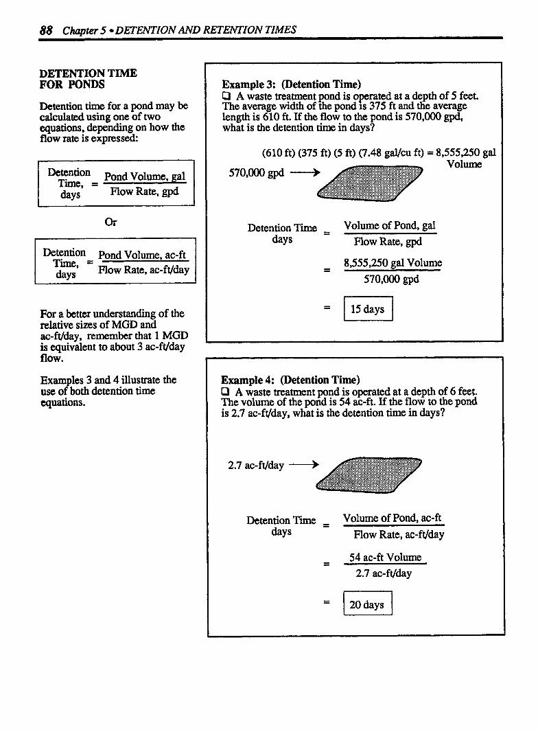
88 C b t e r S DETENTION AND RETENTION TIMES
DETENTION TIME FOR PONDS
Detention time for a pond may be calculated using one of two equations, depending on how the flow rate is expressed:
Detention pond volume, gal Time, = &ys Flow Rate, gpd
Detention Pond Volume, ac-ft Time, = days Flow Rate, ac-ft/day
For a better understanding of the relative sizes of MGD and ac-ft/day, remember that 1 MGD is equivalent to about 3 ac-ft/day flow.
Examples 3 and 4 illustrate the use of both detention time equations.
Example 3: (Detention Time) P A waste treatment pond is operated at a depth of 5 feet. The average width of the pond is 375 ft and the average length is 610 ft. If the flow to the pond is 570,000 gpd, what is the detention time in days?
(610 ft) (375 ft) (5 ft) (7.48 gaVcu ft) = 8,555,250 gal
- - 8,555,250 gal Volume 570,000 gpd
Example 4: (Detention Time) P A waste treatment pond is operated at a depth of 6 feet. The volume of the pond is 54 ac-ft. If the flow to the pond is 2.7 ac-ft/day, what is thc detention time in days?
- 54 ac-ft Volume 2.7 ac-ft/day
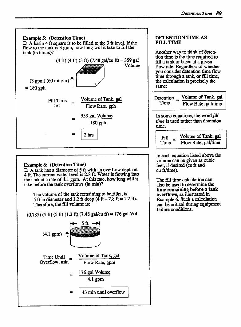
Detention Time 89
Example 5: (Detention Time) LI A basin 4 ft square is to be f111ed to the 3 ft level. If the flow to the tank is 3 gpm, how long will it take to fill the tank (in hours)?
(4 ft) (4 ft) (3 ft) (7.48 gaVcu ft) = 359 gal Volume
Fill Time = Volume of Tank, gal hrs How Rate, gph
- - 359 gal Volume
Example 6: (Detention Time) Q A tank has a diameter of 5 ft with an overflow depth at 4 ft. The current water level is 2.8 ft. Water is flowing into the tank at a rate of 4.1 gpm. At this rate, how long will it take before the tank overflows (in min)?
The volume of the tank remaining to be filled is 5 ft in diameter and 1.2 ft deep (4 ft - 2.8 ft = 1.2 ft). Therefore, the f'ill volume is:
(0.785) (5 ft) (5 ft) (1.2 ft) (7.48 gaVcu ft) = 176 gal Vol.
Time Until = Volume of Tank, gal Overflow, min Flow Rate, gpm
- - 176 gal Volume 4.1 gpm
= / 43 min until oveflow I
DETENTILON TIME AS FILL TIME
Another way to think of &ten- tion time is the t h required to fill a tank or basin at a given flow rate. Regardless of whether you consider detention time flow time through a tank, or fYl time, the calculation is precisely the same:
In some equations, the wordfill tim is used rather than detention time.
ill Volume of Tank, gal Time Flow Rate, gaVtime
In each equation listed above the volume can be given as cubic feet, if desired (cu ft and cu ft/time).
The fill time calculation can also be used to determine the time remaining before a tank overflows, as illustrated in Example 6. Such a calculation can be critical during equipment failure conditions.

90 Chapter 5 DETENTION AND RETENTION TIMES
5.2 SLUDGE AGE CALCULATIONS
Sludge age refers to the average number of days a particle of suspended solids remains under aeration. It is a calculation used to maintain the proper amount of activated sludge in the aeration tank.
When considering sludge age, in effect you are asking, "how many days of suspended solids are in the aeration tank?" If you know how many pounds of suspended solids enter the aeration tank daily and you can determine how many total pounds of suspended solids are in the aeration tank, then you can calculate how many days of solids are in the aeration tank. For example, if 2000 lbs SS enter the aeration tank daily and the aeration tank contains 10,000 lbs of suspended solids, then 5 days of solids are in the aeration tank--a sludge age of 5 days.
Notice the similarity of this calculation with that of detention -sludge age is solids re- tained calculated using units of lbs and lbs/day; detention time is water retained, using units of gal and gaVtime or cu ft and cu ft/time:
Detention - Volume of Tank, gal - Time, min Flow Rate, gpm
SLUDGE AGE IS BASED ON SUSPENDED SOLIDS ENTERING THE AERATION TANK*
lbs/day SS Added 7
Aeration
lbs MLSS in Aeration Tank Simplified Equation:
Sludge Age, - - MLSS, lbs days SS Added, lbs/day
Expanded Equation:
Sludge Age, = (MLSS mg/L) (Aer. Vol., MG) (8.34 lbslgal) days (P. E. S S, mglL) (Flow, MGD) (8.34 lbs/gal)
Example 1: (Sludge Age) P An aeration tank has a total of 13,000 lbs of mixed liquor suspended solids. If a total of 2540 lbs/day suspended solids enter the aeration tank in the primary effluent flow, what is the sludge age in the aeration tank?
13,000 lbs MLSS
Sludge Age - - MLSS, lbs days SS Added, lbs/day
- - 13,000 lbs 2540 lbs/day
* Sludge age based on solids s-g the aeration tank is sometimes referred to as Sludge Age (Gould) to distinguish it from the calculation of Solids Retention Time (or Mean Cell Residence Time), which is based on solids leaving the aeration tank.
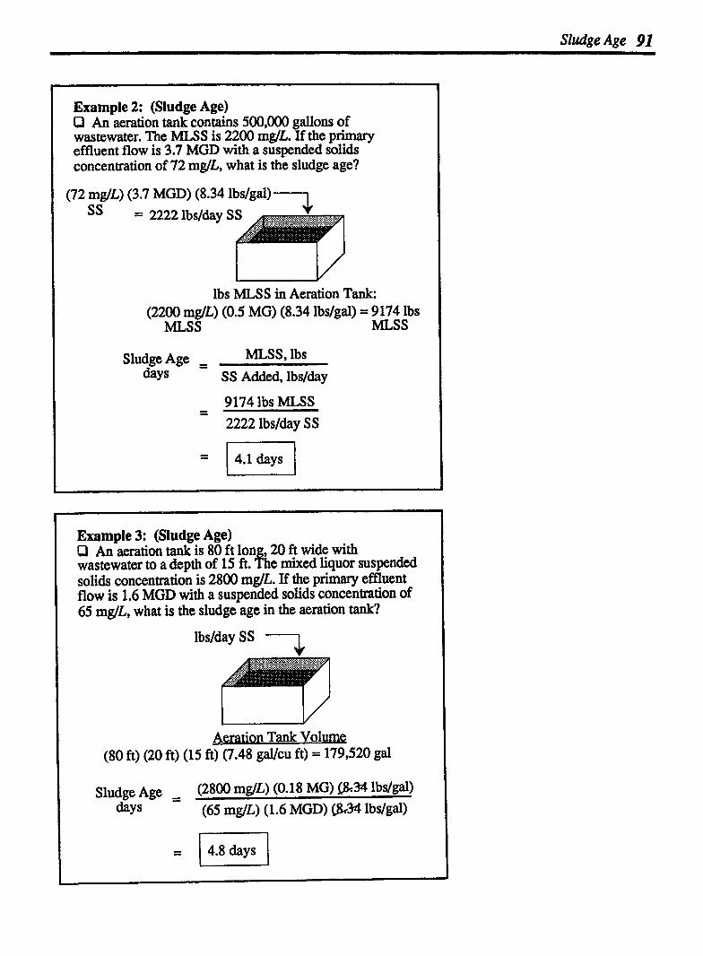
Sludge Age 91
Example 2: (Sludge Age) O An aeration tank contains 500,000 gallons of wastewater. The MLSS is 2200 m& If the primary effluent flow is 3.7 MGD with a suspended solids concentration of 72 mglL, what is the sludge age?
(72 mglL) (3.7 MGD) (8.34 lbslgal) -1
L v
lbs MLSS in Aeration Tank: (2200 mglL) (0.5 MG) (8.34 lbslgal) = 9174 lbs
MISS MLSS
Sludge Age - MLSS, lbs days SS Added, lbslday
- 9174 lbs MLSS 2222 lbslday SS
Example 3: (Sludge Age) LI An aeration tank is 80 ft lon ,20 ft wide with wastewater to a depth of 15 ft. ' h e mixed liquor suspended solids concentration is 2800 m@. If the primary effluent flow is 1.6 MGD with a suspended solids concentration of 65 mglL, what is the sludge age in the aeration tank?
Aeration Tank Volume (80 ft) (20 ft) (15 ft) (7.48 gaVcu ft) = 179,520 gal

92 Chapter 5 DETENTION AND RETENTION TIMES
USING SLUDGE AGE TOCALCULATEOTHER UNKNOWNS
The sludge age equation can be used to calculate:
Desired lbs MLSS, and
Desired mglL SS
In Examples 1-3, sludge age was the unknown variable. In Examples 4-6, the sludge age equation is used to calculate the desired pounds of MLSS in the aeration tank.
Example 4: (Sludge Age) P A slud e age of 5 da S is desired. Assume l200 lbslday suspendsol~ds enter X c aeration tank in the primary effluent To maintain thc desired sludge age, how many lbs of MLSS must be maintained in the aeration tank?
Sludge Age - - MLSS, lbs days SS Added, lbs/day
x Ibs MLSS 5&ys =
l200 lbslday SS Added
Example 5: (Sludge Age) P A sludge a e of 5.2 days is desired for an aeration tank 100 ft long, 4 8 ft wide, Hnth a liquid level of 15 ft. If 1950 lbslday suspended solids enter the aeration tank in the primary effluent flow, how many lbs of MLSS must be maintained in the aeration tank to maintain the desired sludge age?
1950 lb~/&y SS '-1
Sludge Age days
5.2 days
x lbs MLSS V MLSS, lbs
SS Added, l b sby
X lbs MLSS - 1950 lbslday SS Added

Example 6: (Sludge Age) P The 1.3-MGD primary effluent flow to an aeration tank has a suspended solids concentration of 65 mglL. The aeration tank volume is 180,000 gallons. If a sludge age of 6 days is desired, what is the desired MLSS concentration?
lbs MLSS
6days = (X mg/L MLS S) (0.1 8 mg) lbs/gal) (65 mg/L) (1.3 MGD) (H lbs/gal)
After dividing out the 8.34 factor from the numerator and denominator, solve for X:
X = (65) (1.3) (6) 0.18
Example 7: (Sludge Age) P A total of 5500 lbs of MLS S are desired in the aeration tank. What is the desired MLSS concentration (in mg/L) if the aeration tank volume is 250,000 gallons?
MLSS I xmglL l/ (X mg/L MLSS) (0.25 MG) (8.34) = 5 500 lbs MLSS
X = ( 2638 mglL MLSS (
CALCULATING MLSS CONCENTRATION GIVEN POUNDS SOLIDS AND AERATION TANK VOLUME
The sludge age equation can be used in some cases, such as in Example 6, to calculate the actual or desired MLSS concen- tration. However, many times sludge age is not mentioned at all and yet MLSS concentration musi be determined.
When converting from mg/L to lbs MLSS or vice versa, the following equation is used:*
(mg/L) (Vol. MG) (8.34) = lbs lbslgal
Note that this is the same equation used in the sludge age numerator to calculate lbs SS (lbs MLSS) in the aeration tank :
l (mgfL) (Aer.Vo1.) (8.34) = lbs MLSS MG Wgal MLSS
* m& to lbs/&y calculations are discussed in Chapter 3.
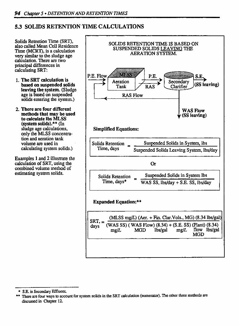
94 Chapter 5 8 DETENTION AND RETENTION TIMES -- -p- - p- - p
5.3 SOLIDS RETENTION TIME CALCULATIONS
Solids Retention Time (SRT), also called Mean Cell Residence Time (MCRT), is a calculation very similar to the sludge age calculation. There are two principal differences in calculating SRT:
1. The SRT calculation is based on suspended solids leaving the system. (Sludge age is based on suspended solids entering the system.)
2. There are four different methods that may be used to calculate 1bs MLSS (system solids).* * (In sludge age calculations, only the MLSS concentra- tion and aeration tank volume are used in calculating system solids.)
Examples 1 and 2 illustrate the calculation of SRT, using the combined volume method of estimating sys tern solids.
SOLIDS RETENTION TIME IS BASED ON SUSPENDED SOLIDS LEAVING THE
AERATION SYSTEM.
I A RAS Flow
WAS Flow (SS leaving)
Simplified Equations:
Solids Retention - Suspended Solids in System, Ibs Time, days Suspended Solids Leaving System, lbslday
Solids Retention - -. Suspended Solids in System lbs
Time, days* WAS SS, lbs/day + S.E. SS, lbs/day
Expanded Equation:**
(MLSS mg/L) (Aer. + Fin. Clar.Vols., MG) (8.34 lbslgal) SRT, =
(WAS SS) ( WAS Flow) (8.34) + (S.E. SS) (Plant) (8.34) days m g / ~ MGD lbdgal mglL flow lbslgal
MGD
* S.E. is Secondary Effluent. ** There are four ways to account for system solids in the SRT calculation (numerator). The other three methods are
discussed in Chapter 12.

Solids Retention Time 95
Example 1: (Solids Retention Time) D An activated slud e system has a total of 9930 lbs of mixed liquor suspen i ed solids. The suspended solids leaving the final clarifier in the effluent is calculated to be 290 lbs/day. The lbs suspended solids wasted from the final clarifer is 1050 lbs/day. What is the solids retention time, in days?
290 lbslday SS
9930 lbs MLSS v l050 lbslday WAS SS
SRT - MLSS in System, lbs days WAS SS, lbs/day + S.E. SS, lbsjday
9930 lbs MLSS -
1050 lbsjday + 290 lbs/day
Example 2: (Solids Retention Time) O An aeration tank has a volume of 330,000 gal. The final clarifier has a volume of 150,000 gallons. The MLSS concentration in the aeration tank is 2900 mglL. If a total of 1520 lbs SSIday are wasted and 400 1bs SSIday are in the secondary effluent, what is the solids retention time for the activated sludge system?
SRT - - MLSS in System, lbs days WAS SS, lbs/day + S.E. SS, lbs/&y
- - (2900 mglL) (0.48 MGD) (8.34 lbslgal) 1520 lbslday + 400 lbslday
- - 1 1,609 lbs MLS S 1920 lbslday SS leaving

96 Chapter 5 DETENTION AND RETENTION TIMES
Example 3: (Solids Retention Time) P Determine the solids retention time (SRT) given the following data:
Aer. Tank Vol. 1.1 MG MLSS 2500 mglL Fin. Clar. Vol. 0.4 MG WAS SS 6150 mglL P.E. Flow 3.9 MGD S.E. SS 15 mglL WAS Pumping Rate 80,000 gpd
MLSS in System, lbs SS Leaving System, lbs/day
(2500 mgL) ( l . 5 MG) (8.34 lbdgal) (6150) (0.08) (8.34) + (15) (3.9) (8.34) mglL MGD lbs/gal mglL MGD lbdgal
3 1,275 lbs MLSS 4103 lbs SS + 488 lbs SS
6.8 days 0 Example 4: (Solids Retention Time) 0 Calculate the solids retention time (SRT) given the following data:
Aer. Tank Vol. 300,000 gal MLSS 2400 m& Fin. Clar. Vol. 120,000 gal WAS SS 5900 mglL P.E. Flow 2.2 MGD S.E. SS 20 m& WAS Pumping Rate 19,000 gpd
SRT , MLSS in System, lbs days SS Leaving System, lbs/day
(2400 mdL) (0.42 MG) (8.34 lbs/gal)
mg/LL MOD- l&/& &L MGD lbs/gal
8407 lbs MLSS
= 1 6.5 days l

Solids Retention Time 97
Example 5: (Solids Retention Time) P The volume of an aeration tank is 320,000 gal and the final clarifier is 130,000 gal. The desired SRT for a plant is 7 days. The primary effluent flow is 2 MGD and the WAS pumping rate is 25,000 gpd. If the WAS SS is 5400 mglL and the secondary effluent SS is 18 mg/L, what is the desired MLSS mg/L?
___) S.E. SS
X m& MLSS * WAS SS
SRT - - MLSS in System, lbs days SS Leaving System, lbs/day
7 days = (X mg/L MLSS) (0.45 MG) (8.34 lbs/gal) (5400) (0.025) (8.34) +(18) (2) (8.34)
7 days = ( X ) (0.45) (8.34) 1126 + 300
CALCULATING OTHER UNKNOWN FACTORS
The SRT calculation incorporates many variables:
SRT
Aeration Tank and Clarifier Volumes
WAS SS, mg/L
WAS Pumping Rate, MGD
S.E. SS, mglL
Plant Flow
In Examples 1-4, SRT was the unknown variable. Other var- iables can also be unknown, as illustrated in Example 5. Regardless of which variable is unknown, use the same equation, fill in the given information, then solve for the unknown value,


Other Percent CalcuZations
1. Unit process efficiency calculations refer to the percent removal of a water or wastewater constituent such as suspended solids (SS) or biochemical oxygen demand (BOD).
Simplified Equation:
Pm Removed % Removed =
Total
S S Removal Efficiencv;
SS in influent ent - (Total SS entering) Aeration Tank d v
SS Removed
SS Removed, mg/L , 100 % SS Removed =
SS Total, mglL
BOD in influent BOD in effluent ______) 1 (Total BOD entering) Aeration Tank /
BOD Removed
I I
I
* To review percent calculations, refer to Chapter 5 in Bark Math Concepts.
l
This chapter focuses on various percent calculations in water and wastewater math. The underlying concept in each of these calculations is percent: *
BOD Removed, mg/L % BOD Removed =
BOD Total, mg/L
% S - x100 Whole
Note that for every percent sign, 96, included in an equation, there should be a l00 factor in the equation as well-either direcdy un&r the percent sign or on the opposite side of the equation in the same relative location. (If the percent sign is in the numerator, the l00 factor on the opposite side of the equation will also be in the numerator. And if the percent sign is in the denominator, the 100 factor on the opposite si& of the equation will also be in the denominator. This can be verified by moving the 100 factor according to the diagonal rule of movement)* * The equation above shows the 100 factor on the opposite side of the equation. Written on the same side of the equation it would be:
% Part -= 100 Whole
This concept of the location of the100 factor is important since you will encounter equations using both means of expression.
** For a reviek of moving terms from one side of the equation to the other, refer to Chapter 2 in Bmic Math Concepts.

100 Chapter 6 EFFICIENCY AND OTHER PERCENT CALCULATIONS
Sludge percent calculations include four different calculations (problem types 2-5 below):
2. Percent Solids and Sludge Pumping R a t e h making these calculations it is important to distinguish between the terms "solids" and "sludge". Solids refers to dry solids; whereas, sludge refers to water solids.*
The two most common sludge percent calculations are percent solids and sludge pumping rate.
Usine laboratory dau:
% Solids = Weight of Solids, grams Total Weight of Sample, grams
.lrn l Using ~ lan t dat~:
% Solids = Solids, lbs/day 100 Sludge, lbslday
The second equation can be used to calculate lbslday or gpd sludge to be pumped. If desired, the equation tin be muranged as follows:
1 (Sludge, lbs/day) = Solids, lbslday % Solids I
+ The diagram of sludge and solids is for illustration purposes only and is not to scale. Primary sludge contains about 3.5% solids, and secondary sludges about 103% solids. Sludge is actually a m of solids and water. The diagram above shows the portions of water and solids if they were separated.

3. Mixing Different Percent Solids Sludges When mixing sludges with different percent solids, use the following equation to calculate the percent solids concentration of the resulting sludge:
% Solids of , solids in Mixture, lbs/day X 100
sludge Mixnue Sludge Mixture, lbs/day
4. Percent Volatile Solids--Two equations represent the two most common volatile solids calculations-the first using laboratory data, the second using plant data.*
r Sludge
% Volatile - Weight Volatile Solids, grams Solids
- Weight of Total Solids, grams
% volatile Volatile Solids, lbs Solids X l r n /
Total Solids, lbs
5. Seed Sludge (Based on 96 Digester Volume) In Chapter 4, required digester seed sludge was calculated on the basis of a volatile solids loading ratio. Another way to calculate seed sludge required is based on a percent of the digester volume.
1 Digester 1
% Seed = Seed Sludge, gal X 100 Sludge Total Digester Capacity, gal
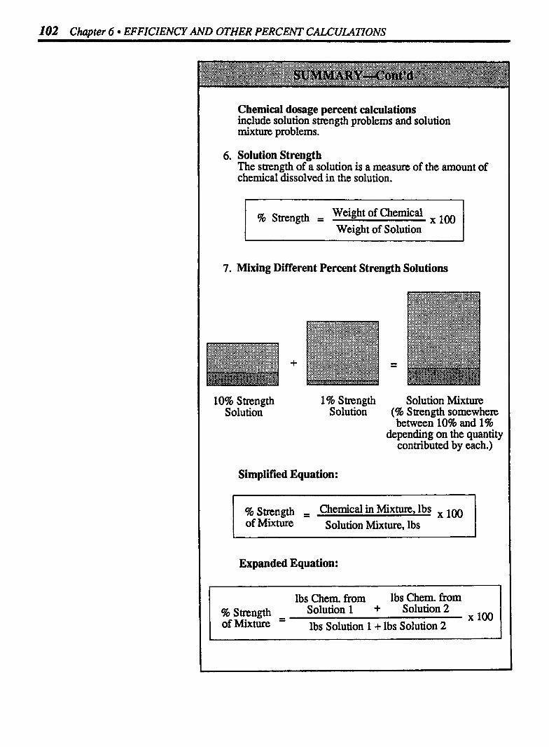
102 Chapter 6 EFFICIENCY AND OTHER PERCENT CALCULATIONS
Chemical dosage percent calculations include solution strength problems and solution mixture problems.
6. Solution Strength The strength of a solution is a measure of the amount of chemical dissolved in the solution.
% Strength = Weight of Chemical Weight of Solution
I 7. Mixing Different Percent Strength Solutions
10% Strength 1% Strength Solution Mixture Solution Solution (% Strength somewhere
between 10% and I% depending on the quantity
contributed by each.)
I Simplified Equation:
% Strength = Chemical in Mixture, lbs of Mixture Solution Mixture, lbs
l Expanded Equation:
I I lbs Chern. from lbs Chem. from I
l I % Strength Solution 1 + Solution 2 of Mixture lbs Solution 1 + lbs Solution 2

8. Pump and motor efficiency calculations are based on horsepower input and output.
% Efficiency = HP Output
100 Hp Input

104 Chapter 6 EFFICIENCY AND OTHER PERCENT CALCULATIONS
6.1 UNIT PROCESS EFFICIENCY CALCULATIONS
The efficiency of a treatment process is its effectiveness in removing various constituents h m the water or wastewater. Suspended solids, BOD and COD removal are the most common calculations of unit process efficiency.
UNIT PROCESS EFFICIENCY IS PERCENT REMOVAL
SS or BOD in influent OD in effluent (Total SS entering)
SS or BOD Removed
% Removed = Part Removed Total
For example, SS removal efficiency is calculated as:
%SS = SS Removed, mglL &moved S S Tot a1 , mglL
Example l: (Unit Process Efficiency) P The suspended solids entering a trickling filter is 190 mglL. If the suspended solids in the trickling filter effluent is 22 mglL, what is suspended solids removal efficiency of the trickling filter?
Total Entering U 168 mg/L
SS Removed
%SS = SS Removed, mglL Removed SS Total, mglL
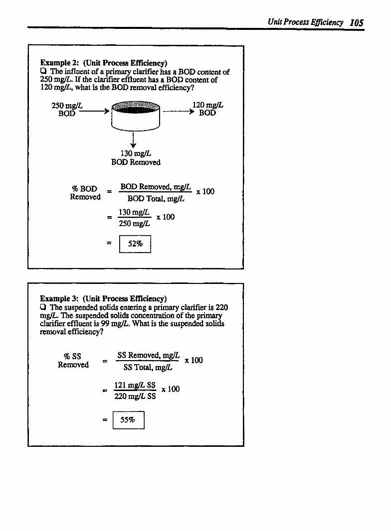
Unit Process Emienncy 105
Example 2: (Unit Process Effidency) P The influent of a primary clarifier has a BOD conttnt of 250 mdL. If the clarifier effluent has a BOD content of 120 mglL, what is the BOD removal efficiency?
25omg/" , 120 mglL BOD B BOD
130 mglL BOD Removed
96 BOD Removed
- - BOD Removed, mglL 100 BOD Total, mglL
Example 3: (Unit Process Efficiency) C1 The suspended solids entering a primary clarifier is 220 mglL. The suspended solids concentration of the primary clarifier effluent is 99 mglL. What is the suspended solids removal efficiency?
% SS 9
9
SS Removed, mglL Removed SS Total, mglL

l06 Chapter 6 EFFICIENCY AND OTHER PERCENT CALCULATIONS
6.2 PERCENT SOLIDS AND SLUDGE PUMPING RATE CALCULATIONS
PERCENT SOLIDS
Sludge is composed of water and solids. The vast majority of sludge is water-usually in the range of 93 to 97%.
To determine the solids content of a sludge, a sample of sludge is dried overnight in an oven at about 103O- 105' C. The solids that remain after drying represent the total d i & &tent of the sludge. This solids content may be expressed as a percent or as a mglL, concentration.* Two equations are used to calculate percent solids, depending on whether lab data or plant data is used in the calculation. In both cases, the calculation is on the basis of solids and sludge weight.
Total Solids, g % Solids =
Sludge Sample, g
Solids, lbs I I Sludge, lbs I
Example 1: (Percent Solids) P The total weight of a sludge sam le is 15 grams. (Sludge sample only, not the dish.) P f the weight of the solids after drying is 0.62 grams, what is the percent total solids of the sludge?
% Solids = Total Solids, grams Sludge Sample, grams
- - 0.62 grams 15 grams
Example 2: (Percent Solids) C l A total of 3000 gallons of slud e is pumped to a digester. If the sludge has a 6% so !I 'ds content, how many lbs/day solids are pumped to the digester?
First, write the % solids equation and fill in the given information:
% Solids = Solids, lbs/day ,100 Sludge, lbdday
xlbs/daySolids xlOO 6 = (3000 gal) (8.34 lbslgal)
- --
* 1% solids = 10,000 mg/L. For a review of W to mg/L conversions, refer to Chapter 8 in Baric Moth Concepts.

Percent Solids 107
Example 3: (Percent Solids) D A total of 10,000 lbslday SS are removed from a primary clarifier and pumped to a sludge thickener. If the sludge has a solids content of 3%, how many lbslday sludge are pumped to the thickener?
Solids, lbslday , % Solids =
Sludge, lbslday
10,000 lbsfday Solids 3 =
X lbslday Sludge
= 1 333,333 lbs/day Sludge
Example 4: (Percent Solids) P It is anticipated that 200 lbslday SS will be pumped from the primary clarifier of a new plant. If the primary clarifier sludge has a solids content of 5%, how many gpd sludge will be pumped from the clarifier? (Assume the sludge weighs 8.34 lbslgal.)
First calculate lbs/day sludge to be pumped using the % solids equation, then convert lbslday sludge to gpd sludge:
Sludge, lbslday = Solids, lbslday % Solids
xlbslday Sludge = 200 lbslday Solids 0.05
X = 4000 lbslday Sludge
Converting lbslday sludge to gpd sludge:
4000 lbslday Sludge 8.34 lbslgal
CALCULATING OTHER UNKNOWN VARIABLES
The three variables in percent solids calculations are percent solids, lbdday solids, and lbdday sludge. In Example 1, percent solids was the unknown variable. Examples 2-4 illustrate calcu- lations when other variables are unknown. In solving these pro- blems, write the equation as usual, fill in the known infor- mation, then solve for the un- known value.*
SLUDGE TO BE PUMPED
As mentioned above, one of the variables in the % solids calcu- lation is lbslday sludge. Example 3 illustrates a calculation of lbsjday sludge. Example 4 illu- strates the calculation of gpd sludge to be pumped.
Because lbslday sludge is calculated relatively frtquently, the % solids equation is often rearranged as follows:
Sludge, = Solids, lbslday lbslday % Solids
100
* Refer to Chapter 2 in Basic Math Concepts for a review of solving for the unknown value.

108 Chapter 6 EFFICWCY AND OTHER PERCENT CALCULATIONS
6.3 MIXING DIFFERENT PERCENT SOLIDS SLUDGES CALCULATIONS
When sludges with different percent solids content are mixed, the resulting sludge has a percent solids content somewhere between the solids contents of the original sludges. For example, if a 4% primary sludge is mixed with a 1% secondary sludge, the resulting sludge might have a solids content of about 2 or 3%. The actual percent solids content will depend on how much (lbs) of each sludge is mixed together. If, in the example, most of the sludge is from the secondary sludge (1% solids) and very little fiom the primary sludge (4% solids), then the resulting sludge would be closer to a 1 % sludge (perhaps a 1 .S% sludge). If, on the other hand, most of the sludge is prknary sludge and very little is secondary sludge, then the resulting sludge mixture might have a solids content closer to 4%-such as 3 or 3.5%.
The actual solids content of a mixtm of two or more sludges depends on the pounds of sludge contributed h m each source.
As with the sludge thickening equation, remember that if the thickened sludge has a density pa t e r than 8.34 lbdgal, it must be used instead of 8.34 lbdgal. *
WHEN SLUDGES ARE MIXED THIE MIXTURE HAS A % SOLIDS CONTENT BETWEEN THE TWO
ORIGINAL % SOLIDS VALUES
5% Primary Sludge 3% Thickened
Secondary Blended Sludge
Sludge (96 Solids ~6mewhen Between 3% and 5%)
Simplified Equation:
% solids of = Solids in Mixture, lbslday sludge Mixture Sludge Mixture, lbs/day
Expanded Equation:
% Solids Prim. Sol., lbslday + Sec. Sol., lbs/day of Sludge = Rim S1 X 100 Mixture . udge, lbslday + Sec. Sludge, lbslday
Example 8: (Mixing Sludges ) O A primary sludge flow of 5000 d (5% solids) is mixed F with a thickened secondary sludge ow of 3500 gpd (3% solids). What is the percent solids content of the mixed sludge flow?
% Prim. S1. Sol., lbslday + Sec. S1. Sol., lbslda~ 100 of Sludge = Prim. Sludge, lbslday + Sec. Sludge, lbs/day
(5000 gpd) (8.34) + (3500 gpd) (8.34) Rim. Sludge Sec. Sludge
- - 2085lbs/dayPrimSol.+876lbs/daySec.Sol. 41,700 lbslday Prim Slud. + 29,190 lbslday Sec. Slud.
- 296 1 lbslday Solids 1m 70,890 lbslday Sludge
= 14.2% Solids I
* Refer to Chapter 7 for a review of density and specific gravity.

Mixing Sludges 109
Example 9: (Mixing Sludges ) P Primary and thickened secondary sludges are to be mixed and sent to the digester. The 5700 gpd primary sludge has a solids content of 5.5%; the 4200 gpd thickened secondary sludge has a solids content of 3.896.What would be the percent solids content of the mixed sludge?
% Solids Prim. S1. Sol., lbslday + Sec. S1. Sol., lbs/&y , 100 of Sludge = ~ i , ~ Prim. Sludge, lbslday + Sec. Sludge, lbslday
(5700 gpd) (8.34) (5.5 ) + (4200 gpd) (8.34) ( 3.8 ) - - Prim. S1. lbslgal 100 Sec. S1. lbs/gal 100 ,
(5700 gpd) (8.34) + (4200 gpd) (8.34) Prim. Sludge lbslgal Sec. Sludge lbslgal
- - 2615 lbs/day Prim Sol. + 133 1 lbslday Sec Sol. , 47,538 lbs/&y Prim. Slud.+ 35,028 lbs/day Sec. Slud.
- - 3946 lbslday Solids 82,566 lbs/&y Sludge
= 14.8% Solids I
Example 10: (Mixing Sludges ) P A rimafy sludge flow of 6800 (3.8% solids) is J F mix with a thickened secondary S udge flow of 4500 gpd (7% solids). What is the percent solids of the combined sludge flow?
Prim. S1. Sol.. lbslday + Sec. S1. Sol., lbslday , of Sludge = ~i~~ Prim. Sludge, lbs/day + Sec. Sludge, lbslday
(6800 gpd) (8.34) ( 3.8 ) + (4500) (8.34) (7) - - Wgal 100 lbslgal 100 , loo
- 2155 lbslday + 2627 lbslday , 100 56,712 lbslday + 37,530 lbslday
- 4782lbsldaySolids , 94,242 lbs/day Sludge
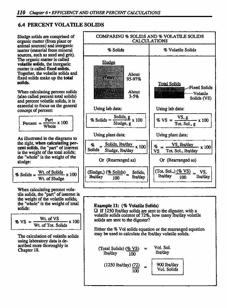
110 Chapter 6 EFFICIENCY AND OTHER PERCENT CALCULATIONS
6.4 PERCENT VOLATILE SOLIDS
Sludge solids are comprised of organic matter (from plant or animal sources) and inorganic matter (material from mineral sources, such as sand and grit). The organic matter is called volatile solids, the inorganic matter is called fixed solids. Together, the volatile solids and fixed solids make up the total solids.
When calculating percent solids (also called percent total solids) and percent volatile solids, it is essential to focus on the general concept of percent:
Part Percent = - X 100
Whole I As illustrated in the diagrams to the right, when calculating per- cent solids, the "part" of interest is the weight of the total solids; the "whole" is the weight of the sludge:
9b Solids = Wt. of Solids 100 Wt. of Sludge
When calculating percent vola- tile solids, the "part" of interest is the weight of the volatile solids; the "whole" is the weight of total solids:
Wt.0fVS %VS =
Wt. of Tot. Solids
The calculation of volatile solids using laboratory data is de- scribed mon thoroughly in Chapter 18.
COMPARING % SOLIDS AND % VOLATILE SOLIDS CALCULATIONS
% Solids
Using lab data:
Solids, g % Solids =
Sludge, g X l W /
Using plant data:
Or (Rearranged as)
(Sludge,) (% Solids) - Solids, lb*~ 100 - lbslday
% Volatile Solids
Using lab data:
%VS = Tot. Sol., g
Using plant data:
VS Tot. Sol., lbs/day
Or (Rearranged as)
(Tot. Sol.,) (% vs) - VS, - lbslaay loo lbs/day
Example 11: (% Volatile Solids) D If 1250 lbslday solids are sent to the di ester, with a
solids are sent to the digester? f volatile solids content of 7296, how many bs/day volatile
Either the % Vol solids equation or the rearranged equation may be used to calculate the lbs/&y volatile solids.
(Total Solids) (% VS) = Vol- sol- lbsl&y 100 l bslday
(12501bslday) (72) - 900 lbslday 100 Vol. Solids - U

% VolatileSolids I l l
Example 12: (96 Volatile Solids) O A total of 3000 gpd sludge is to be pumped to the digester. If the sludge has a 6% solids content with 70% volatile solids, how many lbs/&y volatile solids are pumped to the digester?
(Sludge) (% Solids) (%Vol. Sol.) - vol. sol. Ibslda~ 100 100 - lbslday
Since sludge is given in gpd, 8.34 lbslgal must be added to the equation to convert gpd sludge to lbsfday sludge:*
lbslday Sludge m (~ lud e) (8.34) (96 Solids) (% Vol. Sol.) _ vol. Sol. ,a lbd, ,, 100 - lbsfday
(3000) (8.34) (6J (70) ppd lbslgal 100 Vol. Sol.
Example 13: (% Volatile Solids) O A slud e with 5% solids has a volatile solids content of f 68%. If 1 00 lbslday volatile solids are pumped to the digester (a) how many lbs/day sludge are pumped to the digester? and (b) how many gpd sludge are pumped to the digester? (Assume the sludge weighs 8.34 ibslgal.)
(a) (Sludge) (96 Sol.) (46 Vol. Sol.) = Vol. Sol. lbslday 100 l00 l bslday
(X lbslday Sludge) ( 5 ) (68) = 1 2 0 lbslday 100 100 Vol. Sol.
= I 35,294 lbdday l Sludge
(b) Convert lbslday to gpd:
35,294 lbslday 8.34 lbslgal Sludge
CALCULATING VOLATILE SOLIDS GIVEN SLUDGE DATA
Sometimes you will have lbs/day sludge information and will want to calculate lbs/day volatile solids. When this is the case, you must include the % solids factor in the equation as well, shown in the equation below. In effect, you are calculating lbs/day solids fmt, (using the % Solids factor), then the lbslday Volatile Solids (using the 9b Volatile Solids factor):
l (Sludge) (% - Sol.) (% - L VS)- VS lbslday 100 1 0 lbslday
SOLVING FOR OTHER UNKNOWN FACTORS
The equations shown above can be used to solve for any one of the three or four variables shown. Use the same equation, fill-in the known information, and solve for the unknown variable. Example 13 illustrates this type of calculation.
* For a review of flow conversions, refer to Chapter 8 in Busk Math Concepts.

112 Chapter 6 EFFICIENCY AND OTHER PERCENT CALCULATIONS
6.5 PERCENT SEED SLUDGE CALCULATIONS
There are many methods to determine seed sludge required to start a new digester. One method, discussed in Chapter 4, is to use a volatile solids loading ratiwlbs volatile solids added per lb volatile solids in the digester.
Another method is to calculate seed sludge required based on the volume of the digester. This method is not quite as sensitive to the volatile solids balance in the seed sludge and incoming sludge. Examples 1-4 illustrate this calculation.
Although most digesters have cone-shaped bottoms, for simplicity, it is assumed that the side water depth represents the average digester depth.
Example l: (% Seed Sludge) D A digester has a volume of 350,000 gallons. If the digester seed sludge is to be 22% of the digester volume, how many gallons of seed sludge will be required?*
1 350,000 gallons
22% 1
% Seed = Seed Sludge, gal Sludge Total Digester Volume, gal
22 = xgalseedsludge xlOO 350,000 gal Volume
(350,000 gal) (22) X
100
~77,000 = Seed Sludge
Example 2: (96 Seed Sludge) O A 40-ft diameter digester has a ical water depth of 20 ft. If the seed sludge to be used is 2 ?% of the tank volume, how many gallons of seed sludge will be required?
% Seed = Seed Sludge, gal X 100 Sludge Total Digester Volume, gal
20 = x gal Seed Sludge
X 100 (0.785) (40 ft) (40 ft) (20 ft) (7.48 gaVcu ft)
(0.785) (40 ft) (40 ft) (20 ft) (7.48) (20) = X
100
* For a review of volume calculations, refer to Chapter 11 in Basic Marh Concepts.
% Seed Sludge 11 3
Example 3: (% Seed Sludge) O A digester 50 ft in diameter has a side water depth of 20 ft. If the digester seed sludge is to be 25% of the &gester volume, how many gallons of seed sludge will be required?
% Seed = Seed Sludge, gal 100 Sludge Total Digester Volume, gal
X gal Seed Sludge X 100
25 = (0.785) (50 ft) (50 ft) (20 ft) (7.48 gaVcu ft)
(0.785) (50 ft) (50 ft) (20 ft) (7.48) (25) =
100
Example 4: (% Seed Sludge) P A 40-ft diameter digester has a typical side water depth of 18 ft. If 45,700 gallons of seed sludge are to be used in starting up the digester, what percent of the digester volume will be seed sludge?
% Seed = Seed Sludge, gal X 100 Sludge Total Digester Volume, gal
45,700 gal Seed Sludge X = X 100
(0.785) (40 ft) (40 ft) (18 ft) (7.48 gaVcu ft)
CALCULATING OTHER UNKNOWN FACTORS
The= are three variables in percent seed sludge calculations: percent seed sludge, gallons seed sludge, and total gallons digester volume.
In Examples 1-3, the unknown factor was seed sludge gallons. However, the same equation can be used to calculate either one of the other two variables. Example 4 is one such calculation.
114 Chapter 6 EFFICIENCY AND OTHER PERCENT CALCULATIONS
6.6 PERCENT STRENGTH OF A SOLUTION CALCULATIONS
PERCENT STRENGTH USING DRY CHEMICALS
The strength of a solution is a measure of the amount of chemical (solute) dissolved in the solution. Since percent is calculated as "part over whole,"
pexcent strength is calculated as part chemical, in lbs, divided by the whole solution, in lbs:
% Stxength = Chem., lbs 100 Sol'n, lbs
The denominator of the equation, lbs solution, includes both chemical (lbs) and water (lbs). Therefore, the equation can be written in expanded form as:
% = Chem, lbs Strength Water, + Chem.,
lbs lbs
As the two equations above illustrate, the chemical added must be expressed in pounds. If the chemical weight is expressed in ounces (as in Example 1) or grams (as in Example 2), it must first be converted to pounds (to comspond with the other lbs terms in the equation) before percent strength is calculated.
TWO PARTS OF A SOLUTION
@ SOLUTE Chemical to be added
G liquid
@ SOLVENT
SOLUTION
Example l: (Percent Strength) P If a total of 8 ounces of dry polymer are added to 10 gallons of water, what is the percent strength (by weight) of the polymer solution?
Before calculating percent strength, the ounces chemical must be converted to lbs chemical:*
8 ounces = 0.5 lbs chemical
16 ounces/pound
Now calculate percent strength:
% Strength = Chemical, lbs X loo
Water, lbs + Chemical, 1bs
- 0.5 lbs Chemical X 100 (10 gal) (8.34 lbs/gal) + 0.5 lbs
0.5 lbs Chemical 100 83.9 lbs Solution
* To review ounces to pounds conversions refer to Chapter 8 in Basic Math Concepts.
Percent Strength 11 5
Example 2: (Percent Strength) P If 100 grams of dry polymer are dissolved in 5 gallons of water, what percent strength is the solution? (1 g = 0.0022 lbs)
First, convert grams chemical to pounds chemical. Since 1 gram equals 0.0022 lbs, 100 grams is 100 times 0.0022 lbs:
(100 grams) (0.0022 lbs/gram) = 0.22 lbs Chemical Chemical
Now calculate percent strength of the solution:
% Strength = lbs Chemical X 100
lbs Water + lbs Chemical
- - 0.22 lbs Chemical (5 gal) (8.34 lbslgal) + 0.22 lbs
- - 0.22 lbs 100 4 1 .g2 lbs
Example 3: (Percent Strength) O How many pounds of olymer must be added to 25 91 gallons of water to make a o polymer solution?
First, write the equation as usual and fill in the known information. Then solve for the unknown.*
% Strength = lbs Chemical X 100
lbs Water + lbs Chemical
x lbs Chemical 1 = X loo
(25 gal) (8.34 lbs/gal) + x lbs Chemical
--- / 2.1 lbn Chem. / = x
WHEN GRAMS CHEMICAL ARE USED
The chemical (solute) to be used in making a solution may bt measured in grams rather than pounds or ounces. When this is the case, convert grams of chemical to pounds of chemical b e f o ~ calculating percent strength. The following conversion equations may be used:
I l g = 0.0022 lbs
1 lb = 454 grams ** I
SOLVING FOR OTHER UNKNOWN VARIABLES
In the percent strength equation there are three variables: percent strength, lbs chemical and lbs water. In Examples 1 and 2, the unknown value was percent strength. However, the same equation can be used to determine either of the other two variables. Example 3 illustrates this type of calculation.
Note that gallons water can also be the unknown variable in percent strength calculations. First set lbs water as the unknown variable in the equation. Then when you have calculated the lbs water required, you can then convert lbs water to gallons water using the 8.34 lbsfgal factor.
* To review solving for the unknown value, refer to Chapter 2 in Basic Math Concepts. * * If the box method of conversions is used (see Chapter 8 in Basic Math Concepts), both numbers in the
conversion equation must be greater than one.

11 6 Chapter 6 EFFICIENCY AND OTHER PERCENT CALCULATIONS
6.7 MIXING DIFFERENT PERCENT STRENGTH SOLUTIONS CALCULATIONS
Then are two types of solution mixtun calculations. In one type of calculation, two solutions of different strengths are mixed, with no particular target solution strength. The calculation involves determining the percent strength of the solution mixture. These calculations are similar to the sludge mixture problems described in Section 6.3.
The second type of solution mixture calculation includes a desired or target strength. This calculation is described in Chapter 14, Section 5.
WHEN DIFFERENT % STRENGTH SOLUTIONS ARE MIXED
10% Strength Solution
Simplified Equation:
1% Strength Solution Mixture Solution (% Strength somewhere
between 10% and 1 % )
Strength = lbs Chemical in Mixture 100 of Mixture lbs Solution Mixture
Expanded Equations:
I lbs Chem. from lbs Chem. from % Strength - Solution 1 + Solution 2 of Mixture - X 100
lbs Solution 1 + lbs Solution 2
(Soh l)(% Strength) + (Soh 2) (% Strength) % Strength - lbs 100 lbs of Mixture loo X l00
lbs Solution 1 + lbs Solution 2
Example 7: (Solution Mixtures) P If 20 lbs of a 10% stren th solution are mixed with 50 lbs of 1% strength solution, W at is the percent strength of the solution mixture?
% lbs Chem. Erom lbs Chem. fkom
% Strength - Solution 1 + Solution 2 of Mixture - X 100
lbs Solution 1 + lbs Solution 2
(20 lbs) + (50 lbs) (l) - - 100
20 1bs + 50 1bs loo X loo
- - 2 1bs + 0.5 1bs 100 70 lbs
- 2.5 lbs - - X100 70 lbs

Solution Mimres 11 7
Example 8: (Solution Mixtures) Q If 5 gallons of an 8% strength solution are mixed with 40 gallons of a 0.5% strength solution, what is the percent strength of the solution mixture? (Assume the 8% solution weighs 9.5 lbslgal and the 0.5% solution weighs 8.34 lbslgal.)
lbs Chem. from lbs Chem. from % Stxength Solution 1 + Solution 2 of Mixture lbs Solution 1 + lbs Solution 2
(5 gal) (9.5 lbslgal) + (40 gal) (8.34 lbslgal) - - 100 loo X 100
(5 gal) (9.5 lbslgal) + (40 gal) (8.34 lbslgal)
- - 3.8 lbs Chem. + 1.7 lbs Chem. 47.5 lbs Soln 1 + 333.6 lbs Soh 2
LI - 5.5 lbs Chemical , 38 1.1 lbs Solution
= 1 1.4% Strength I
Example 9: (Solution Mixtures) O If 15 gallons of a 10% strength solution are added to 50 gallons of 0.8% strength solution, what is the percent strength of the solution mixture? (Assume the 10% strength solution weighs 10.2 lbs/gal and the 0.8% strength solution weighs 8.8 lbslgal.)
lbs Chem. fiom lbs Chem. fiom % Strength - Solution1 + Solution2 of Mixture ' X 100
lbs Solution 1 + lbs Solution 2
(1 5 gal) (10.2 lbslgal) + (50 gal) (8.8 lbslgal) (0.J - 100 loo X loo
(1 5 gal) (10.2 lbslgal) + (50 gal) (8.8 lbslgal)
- - 15.3 lbs Chem. + 3.5 lbs Chem. , 153 lbs Soln 1 + 440 lbs Soln 2
- - 18.8 lbs Chemical , 593 lbs Solution
USE DIFFERENT DENSITY FACTORS WHEN APPROPRIATE
Percent strength should be expressed in terms of pounds chemical per pounds solution. Therefore, when solutions are expressed in terms of gallons, the gallons should be expnssed as pounds before continuing with the percent strength calculation. It is important to consider what density factor should be used to convert from gallons to pounds. If the solution has a density the same as water, 8.34 lbs/gal would be used. If, however, the solution has a higher density, such as for some polymer solutions, then a higher density factor should be used. When the density is unknown, sometimes it is possible to weigh the chemical solution to determine its density.
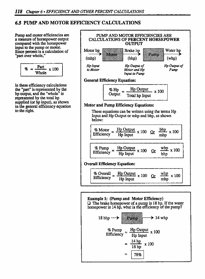
118 Chapter 6 EFFICIENCY AND OTHER PERCENT CALCULATIONS
6.5 PUMP AND MOTOR EFFICIENCY CALCULATIONS
Pump and motor efficiencies are a measure of horsepower output compared with the horsepower input to the pump or motor. Since percent is a calculation of "part over whole,"
in these efficiency calculations the "part" is represented by the hp output, and the "whole" is represented by the total hp supplied (or hp input), as shown in the general efficiency equation to the right
PUMP AND MOTOR EFFICIENCIES ARE CALCULATIONS OF PERCENT HORSEPOWER
OUTPUT
Hp Input to Motor
Hp Output of Hp Output of pump Motor and Hp
Input to Plwzp
General Efficiency Equation:
%Hp - - HP Output X l* Output Total hp Input
pp
Motor and Pump Efficiency Equations: These equations can be written using the terms Hp Input and Hp Output or rnhp and bhp, as shown below:
Overall Efficiency Equation:
%Overall Hp Output lm a Efficiency - HP hput * x l 0 0
mhp
Example 1: (Pump and Motor Efficiency) Cl The brake horsepower of a pum is 18 hp. If the water F horsepower is 14 hp, what is the ef iciency of the pump?
% Pump Hp Output Efficiency - hput

Pump and Motor Eficiency 119
Example 2: (Pump and Motor Efficiency) Q If the motor horsepower is 25 h and the brake horsepower is 22 hp, what is the e f! iciency of the motor?
%Motor - HpOutput 100 Efficiency Input
Example 3: (Pump and Motor Efficiency) P The brake horsepower is 13.5 hp. If the motor is 90% efficient, what is the motor horsepower?
13.5 bhp 90 =
X mhp
Example 4: (Pump and Motor Efficiency) P A total of 20 hp is supplied to a motor. If the wire-to-water efficiency of the pump and motor is 65%, what will the whp be?
X whp I
65% Efficient
X whp 65 = X 100
20 mhp
CALCULATING OTHER UNKNOWN VALUES
Pump and motor efficiency calculations have three variables: efficiency, hp output, and hp input. In Examples 1 and 2, efficiency was the unknown term. However, any one of the variables can be the unknown term as long as data is given for the other two. Example 3 illustrates this type of calculation.
WIRE-TO-WATER EFFICIENCY
Wire-to-water efficiency is another name for overall efficiency of the pump and motor. In other words, thc pump and motor are considered one unit. The hp input to the "unit" is the motor horsepower (mhp); the hp output to the "unit" is water horsepower (whp).

f Pumping Calculations
1. Density and Specific Gravity
The density of a substance is mass per volume (cu ft).
Density of Water = 62.4 lbs
cu ft
Density of any Substance - cu ft
The density of liquids is commonly expressed as pounds per gallon:
Density of - lbs of Liquid a - 1 gal of Liquid
The spccific gravity of a liquid is the density of the liquid compared to the density of water.
I s~ecific Densitv of the Liauid 1
If the specific gravity of a liquid is known, the density of that liquid may be calculated as:*
(Spec. Grav.) (Density) = Density of of a liquid of Water. the Liquid,
62.4 lbs/gal lbs/gal
The specific gravity of a gas is the density of the gas compared to the density of air.
Specific Density of the Gas of = Density of Air
a Gas
Pumping calculations include a variety of different types of problems including:
Density and Specific Gravity,
Pressure and Force,
Head and Head Loss,
Horsepower, and
Pump Capacity.
* Note that this equation is simply the specific gravity equation with the terms rearranged.

122 Chapter 7 PUMPING CALCULATIONS
2. Pressure and Force
Pressure exerted by solid objects depends on contact area.
Force
Pressure = - Area Force l
Pressure exerted by a liquid depends on both liquid depth and density.
I Ressure = (depth) (Density) 1
Since d and D may be confused, the depth is generally expressed as height, h:
Pressure = m E3

2. Pressure and Forcdont 'd
The total force on a surface is the sum of all unit pressures - against it. The total force against the bottom of a tank is:
= (Pressure) (h) Force, lbslsq ft sq ft
lbs
Total = (Pressure) (Area) Force, ibsfsq in. sq in.
lbs
The total force against the side of a tank is:
Total = (Pressure at Average) (Total Area) Force, Depth, lbsfsq ft Q ft
lbs
Total = (Pressure at Average) (Total Area) Force, Depth, lbslsq in. sq in.
lbs
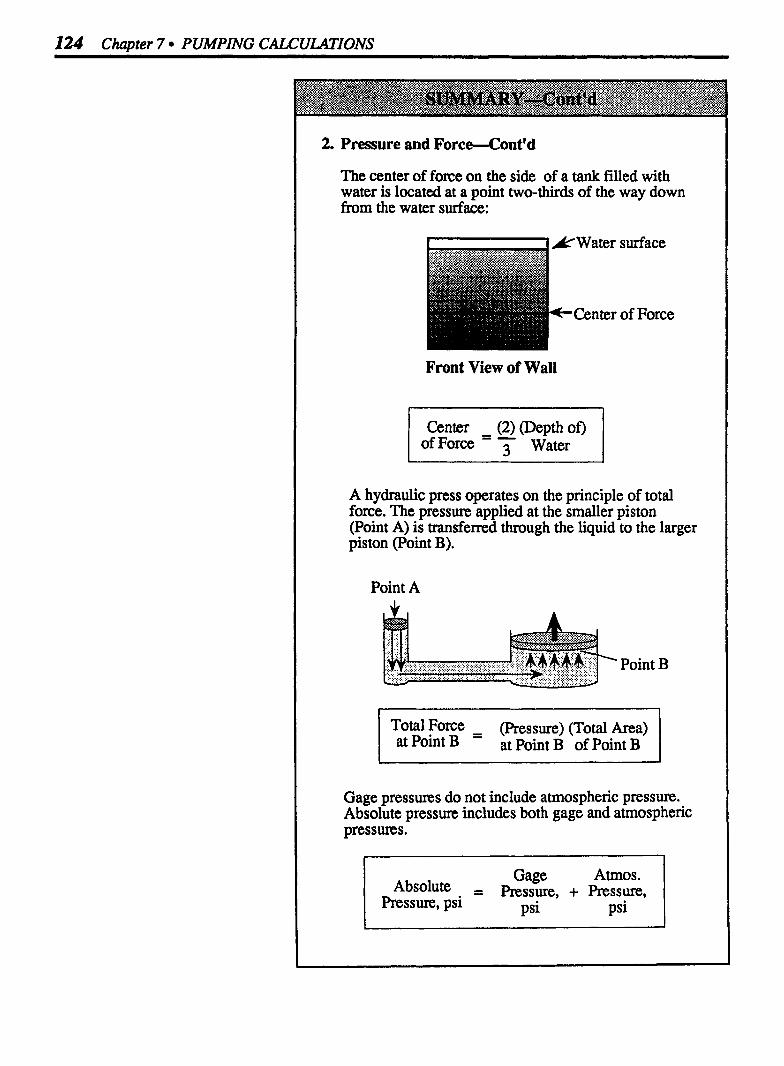
124 Chapter 7 PUMPING CALCULATIONS
2. Pressure and Force-Contfd
The center of force on the side of a tank filled with water is located at a point two-thirds of the way down from the water surface:
Front View of Wall
Center - (2) (~cpth 00 I of Force - -j- Water
A hydraulic press operates on the principle of total force. The pressure applied at the smaller piston (Point A) is transferred through the liquid to the larger piston (Point B).
Point A
Total Force - (Res sure) (Total Area) at Point B - at Point B of Point B
Gage pressures do not include atmospheric pressure. Absolute pressm includes both gage and atmospheric pressures.
Gage Atmos. = Pressure, + ~ ~ ~ s s u r e ,
Pressure, psi psi psi

3. Head and Head Loss
When the two water surfaces are located above the pump, static head is the difference in water surface elevations:
Total Static = Higher - Head, ft Elevation, ft Elevation, ft
lower I When the water surface on the suction side of the pump is below the pump centerline, the two distances must be added:
Height Distance Total Static = Above Pump + Below Pump
Head, ft Centerline, ft Centerline, ft

126 Chapter 7 PUMPING CALCULATIONS
3. Head and Head L o s d o n t ' d
Dynamic head is the static head plus fiction and minor head losses:
Additional head required to compensate for fkiction and minor 1 - head losses t I I
Pump On
Total Dynamic = Total Static + Head Losses Head, ft Head, ft ft
Friction and minor head losses may be determined using hydraulics tables, such as those shown in this chapter.
4. Horsepower
The foundation of all horsepower problems is power- ft-lbs/min:
ft X lbs = ft-lbs min min I - - l

Motor, brake, and water horsepower are terms used to indicate where the horsepower is measured.
Partial Partial Loss of hp Loss of hp
The equations for motor, brake, and water horsepower are:
--- -
Water hp Brake hp = r Pump Effic.
100
Brake hp Motor hp =
Motor Effic.
Motor , - Water hp hp (Motor Effic.) (Pump Effic .)
Each of the three equations above may be rearranged as follows:
Water hp = (Brake hp) (Pump Effic.) loo
Brake hp = (Motor hp) (Motor Effic.) 100
/ Water hp = (Motor hp) (Motor) (Pump) Effic. Effic. -- l

128 Chapter 7 PUMPING CALCULATIONS
4. Horsepower-Cont'd
When pumping liquids with a specific gravity different than that of water, the specific gravity factor must be added to the ft-lbslmin calculation:
(ft) (l bs/min) (spec. grav) = ft-l bs/min for different
1 liquid I
To calculate pumping costs, first calculate the kilowatt-hours ( k m ) power consumption:
(kW)(Hrs of Pump) = kWh draw Operation power
consumed
Then determine pumping cost:
( k W ) (Cost/kWh) = Total Power Use Use Cost
5. Pump Capacity
These calculations are based on a volume of wastewater or sludge pumped during a specific time period The two general types of pumping rate calculations include:
Pumping into or out of a tank, and
Positive displacement calculations
General Equation:
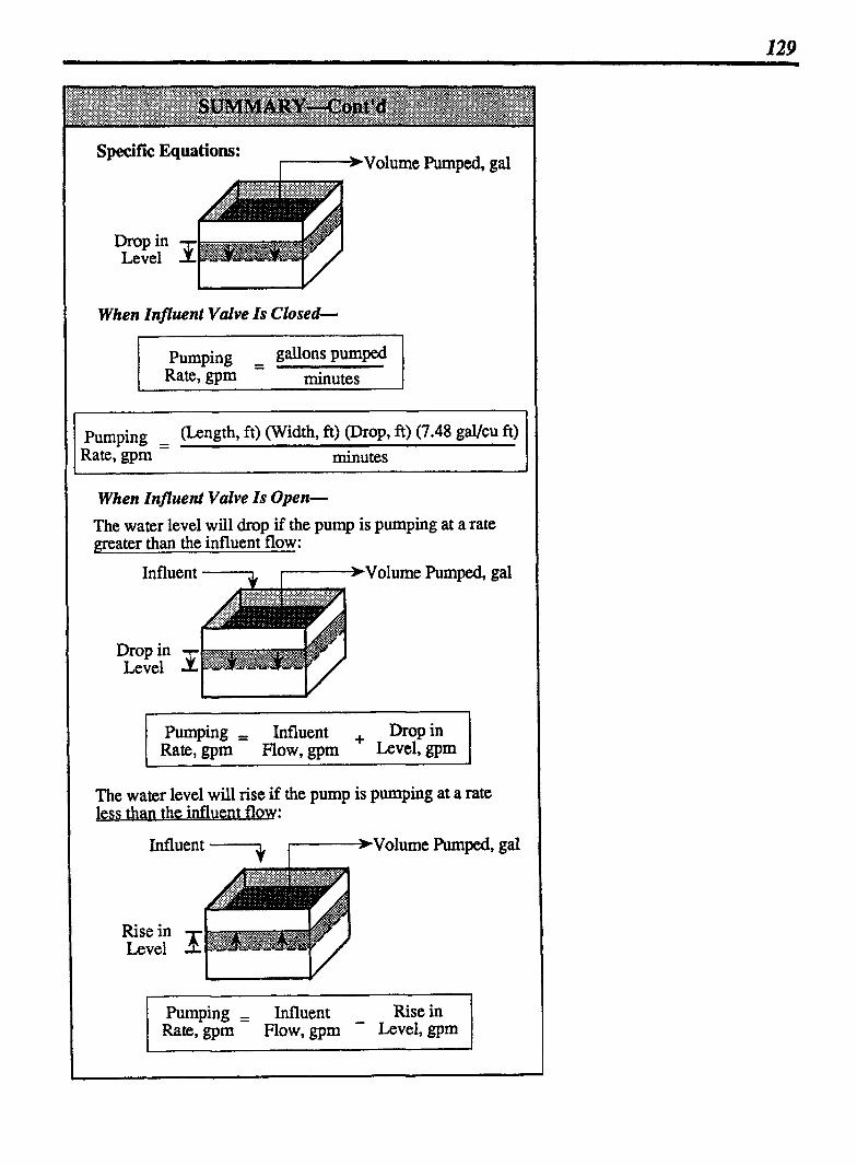
Specific Equations: -Wolume Pumped, gal
Drop Level in X I I/
When Influent Valve Is Closed-
Pumping - - gallons pumped Rate, gpm minutes
When Influent Valve Is Open-
The water level will drop if the pump is pumping at a rate greater than the influent flow:
Influent ,-h (*Volume Pumped, gal
Drop in Level X
Pumping = Influent + 1 Rate, gpm Flow, gpm Level, Drop gpm in I The water level will rise if the pump is pumping at a rate less than the influent flow:
Influent - -*Volume Pumped, gal
Pumping = Influent - Rise in Rate, gprn Flow, gpm Level, gpm

130 Chapter 7 PUMPING CALCULATIONS
7.1 DENSITY AND SPECIFIC GRAVITY
DENSITY
The "lightness" or "heaviness" of an object is the layman's term for what scientists refer to as the density of an object. For example, petrified wood is heavy when compared to volcanic ash, and lead is heavy compared to aluminurn, Such comparisons presume a given volume. That is, any given volume of lead is heavier than the same volume of aluminurn. Without keeping volume constant, no comparison between objects or substances may be made.
The density of a substance is therefore the amount of matter or "mass" in a given volume of that substance. It is normally measured in lbslcu ft. Tables listing the densities of a variety of substances are available in chemical and engineering handbooks. A listing of a few substances is given -
below.
Density Substance ( ~ ~ s / c u fi)
Water 62.4 Seawater 64 Gasoline 44 Aluminurn 170 Lead 700 Wood, pine 30
In the water and wastewater field, the density of water and other liquids is commonly measured in lbslgal. This is simply another expression of mass per unit volume.
DENSlTY IS MEASURED IN LBS/CU FT OR LBSIGAL
The density of water The density of water is 62.4 lbslcu fi is 834 lbslgal
Example l: (Density and Specific Gravity) Q A allo on of solution is weighed. After the weight of the contamer is subtracted, it is determined that the weight of the solution is 9.8 lbs. What is the density of the solution?
lbs of Solution = gal of Solution
Example 2: (Density and Specific Gravity) Q Suppose that only a half a gallon had been wei hed in
would density be calculated? f the example above, with a resulting weight of 4.9 bs. How
lbs of Solution = gal of Solution
4.9 lbs - - 0.5 gal
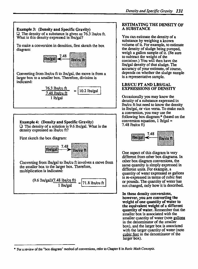
Density and Specific Gravity 131
l Example 3: (Density and Specific Gravity) Cl The density of a substance is given as 76.3 lbs/cu ft.
, What is this density expressed in lbslgal?
To make a conversion in densities, first sketch the box diagram:
Converting from lbs/cu ft to lbslgal, the move is from a larger box to a smaller box. Therefore, division is indicated:
Example 4: (Density and Specific Gravity) O The density of a solution is 9.6 lbs/gal. What is the density expressed as lbslcu ft?
First sketch the box diagram:
Converting from lbs/gal to lbs/cu ft involves a move from the smaller box to the larger box. Therefore, multiplication is indicated:
(9.6 lbs/gal)(7.48 lbslcu ft) l lbslgal
ESTIMATING THE DENSITY OF A SUBSTANCE
You can estimate the density of a substance by weighing a known volume of it. For example, to estimate the density of sludge being pumped, weigh a gallon sample of it. (Be sure to subtract the weight of the container.) You will then have the lbslgal density of that sludge. The accuracy of your estimate, of course, depends on whether the sludge sample is a =presentative sample.
LBSICU FT AND LBSIGAL EXPRESSIONS OF DENSITY
Occasionally you may know the density of a substance expressed in lbs/cu ft but need to know the density in lbs/gal, or vice versa To make such a conversion, you may use the following box diagram:* (based on the conversion equation, 1 lblgal = 7.48 ibsfcu ft)
One aspect of this diagram is very different fkom other box diagrams. In other box diagram conversions, the same quantity is simply expressed in different units. For example, a quantity of water expressed as gallons is reexpressed in terms of cubic feet or pounds. The quantity of water has not changed, only how it is described
In these density conversions, however, you are converting the weight of one quantity of water to the equivalent weight of a different quantity of water. Remember that the smaller box is associated with the smaller quantity of water (note gallong in the denominator of the smder box), and the larger box is associated with the larger quantity of water (note cubic feet in the denominator of the larger box).
* For a review of the "box diagramn method of conversions, refer to Chapter 8 in Basic Math Concepts.
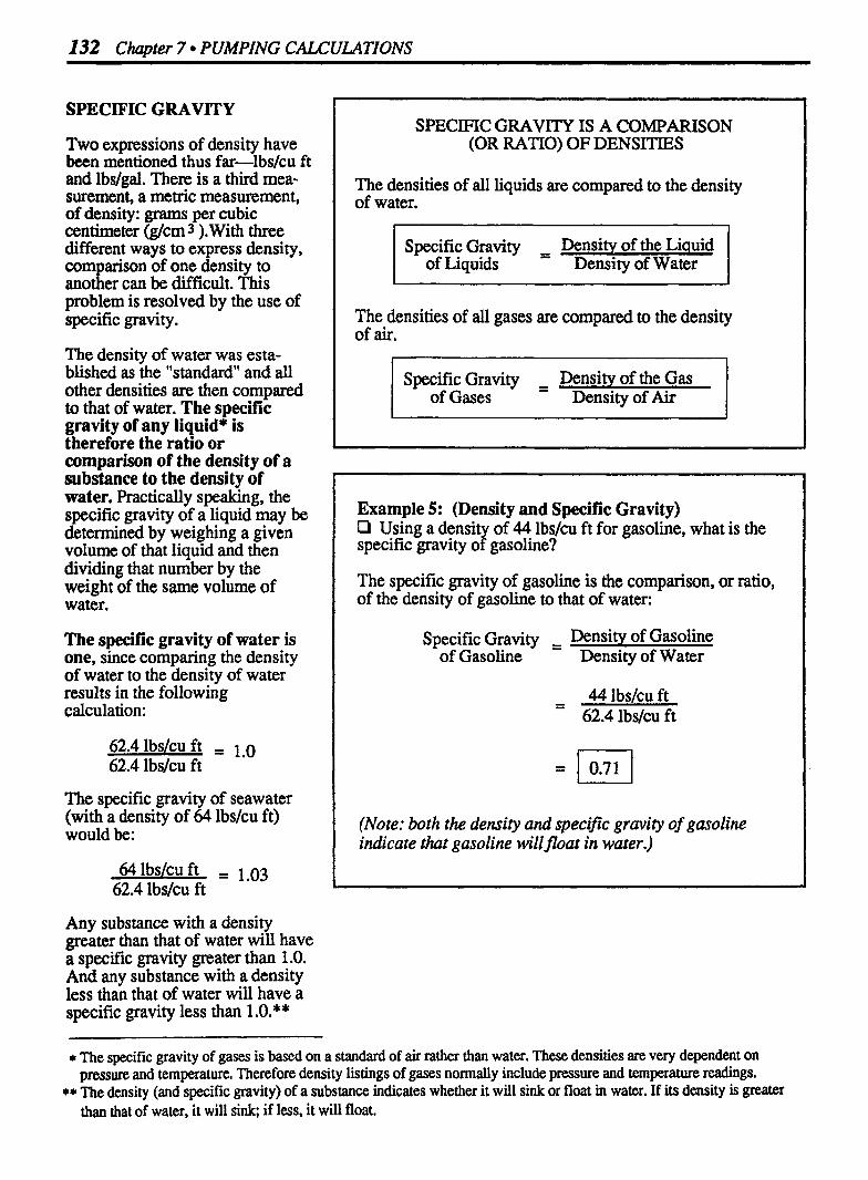
132 Chapter 7 PUMPING CALCULATIONS
SPECIFIC GRAVITY
Two expressions of density have been mentioned thus far-lbs/cu ft and lbslgal. There is a third mea- surement, a metric measurement, of density: grams per cubic centimeter (%cm 3 ).With three different ways to express density, comparison of one density to another can be difficult. This problem is resolved by the use of specific gravity.
The density of water was esta- blished as the "standard" and all other densities are then compared to that of water. The specific gravity of any liquid* is therefore the ratio or comparison of the density of a substance to the density of water. Practically speaking, the specific gravity of a liquid may be determined by weighing a given volume of that liquid and then dividing that number by the weight of the same volume of water.
The specific gravity of water is one, since comparing the density of water to the density of water results in the following calculation:
The specific gravity of seawater (with a density of 64 lbslcu ft) would be:
Any substance with a density greater than that of water will have a specific gravity greater than 1.0. And any substance with a density less than that of water will have a specific gravity less than 1 .O.**
SPECIFIC GRAVITY IS A COMPARISON (OR RATIO) OF DENSITIES
The densities of all liquids are compared to the density of water.
p-
Specific Gravity - Density of the Liquid of Liquids - Density of Water
The densities of all gases are compared to the density of air.
Specific Gravity - Density of the Gas of Gases - Density of Air
Example 5: (Density and Specific Gravity) O Using a densit of 44 lbs/cu ft for gasoline, what is the specific gravity o r gasoline?
The specific gravity of gasoline is the comparison, or ratio, of the density of gasoline to that of water:
Specific Gravity - - Density of Gasoline of Gasoline Density of Water
- - 44 Ibs/cu ft 62.4 lbslcu ft
(Note: both the density and specific gravity of gasoline indicate that gasoline willfloat in water.)
* The specific gravity of gases is based on a standard of air rather than water. These densities are very dependent on pressure and temperature. Therefore density listings of gases normally include pressure and temperature readings.
** The density (and specific gravity) of a substance indicates whether it will sink or float in water. If its density is greater than that of water, it will sink; if less, it will float.

Density and Specific Gravity 133
Example 6: (Density and Specific Gravity) P You wish to determine the specific Pty Of a solution. After weighing a gallon of so ution and subtracting the weight of the container, the solution is found to weigh 9.17 lbs. What is the specific gravity of the solution?
To determine the specific gravity of the solution, its density must be first be determined. Since one gallon of the solution weighed 9.17 lbs, the density is 9.17 lbslgal.
Now compare the density of the solution to that of water to determine specific gravity:
Density of the Solution Specific Gravity = Density of Water
Example 7: (Density and Specific Gravity) P The specific gravity of a liquid is 0.95. What is the density of that liquid?@ensity of water = 8.34 lbslgal).
The specific gravity of a liquid can be used to detennine its density. Multiply the specific gravity times the density of water
(Spec. Grav.) (Density) = Density of the Liq. of water of the
Liquid
DETERMINING THE SPECIFIC GRAVITY OF A SUBSTANCE
To determine the specific gravity of a substance, you must first determine its density (described on the pnvious two pages). Then the density of that sub- stance is compared to the density of water. Example 6 illustrates such a problem.
WHEN SPECIFIC GRAVITY IS KNOWN AND DENSITY IS UNKNOWN
If you know the specific gravity of any substance, you can always determine its density by multiplying the specific gravity by the density of water:
(Specific) (Density) = Density Gravity of Water, of the
ofa always Liquid, Liquid 8.34 lbslgal lbslgal
Example 7 illustrates this type of calculation.

134 Chapter 7 PUMPING CALCULATIONS
7.2 PRESSURE AND FORCE
Force is a push or pull measured in terms of weight, such as pounds or kilograms. The force on the bottom of an open tank, for example, is a measure of the weight of the water above it. The deeper the water, the more force on the bottom of the tank.
Although the force exerted against the entire tank bottom is an important calculation, we will fim focus on another calculation related to force-that of pressure.
Pressure is a measure of the force or weight pushing against a specified area, usually a square inch or a square foot. Thus, pressure is normally expressed in pounds per square inch (lbslsq in. or psi) or pounds per square foot (lbs/sq ft). The general equation used in calculations of pressure is:
Pressure = - Area Foxe l
PRESSURE DEPENDS ON CONTACT AREA
7 lbs
in.
2in 4 in.
7 lbs I
h\-\ 4 in. A brick is set on a table, as shown. A brick is placed on a table, as If the 7 lbs of force (weight) is shown. Now the 7 lbs of force spread over the 32 sq in. of its (weight) is spread over the 8 sq in. side;* the pressure against the of its bottom. The pressure against table at the point of contact is: the table at the point of contact is:
32 sq in. 8 sq in.
Example l: (Pressure and Force) D The object shown below weighs 30 lbs. What is the lbslsq in. pressure at the surface of contact?
Pressm = - Area Force l
Because lbslsq in. pressure is desired, the dimensions will be expressed in inches rather than ft:
Pressure = 30 lbs
(12 in.)(18 in.)
* For a review of area calculations, refer to Chapter 10, "Area Measurements", in Busk Moth Concepts.
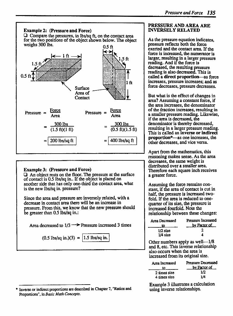
Pressure and Force 135
Example 2: (Pressure and Force) O Compare the pressures, in lbs/s ft, on the contact area for the two positions of the object S own below. The object weighs 300 lbs.
a 0.5 ft
I Force Pressure = - Area
\ surface Area of Contact
- 300 lbs - (1.5 ft)(l ft)
Force PTessUre = - Area
- 300 lbs - (0.5 ft)(1.5 ft)
Example 3: (Pressure and Force) O An object rests on the floor. The pressure at the surface of contact is 0.5 lbs/sq in.. If the object is placed on another side that has only one-third the contact area, what is the new lbslsq in. pressure?
Since the area and pressure are inversely related, with a decrease in contact area there will be an increase in pressure. From this, we know that the new pressun should be greater than 0.5 lbslsq in.:
I Area decreased to 113 +Pressure increased 3 tims
(0.5 lbs/sq in.)(3) = ( 1.5 lbslsq in. I l
-- -
* Inverse or indirect proportions are described in Chapter 7. "Ratios and Proportions", in Baric Math Concepts.
PRESSURE AND AREA ARE INVERSELY RELATED
As the pressure equation indicates, pressure reflects both the force exerted and the contact area. If the force is increased, the numerator is larger, ~sulting in a larger pressure reading. And if the force is decreased, the resulting pressure reading is also decreased. This is called a direct proportion-as force increases, pressure increases; and as force decreases, pressure decreases.
But what is the effect of changes in area? Assuming a constant force, if the area increases, the denominator of the fraction increases, resulting in a smaller pressure reading. Likewise, if the area is decreased, the denominator is thereby decreased, resulting in a larger pressure reading. This is called an inverse or indirect proportion*-as one increases, the other decreases, and vice versa.
Apart from the mathematics, this reasoning makes sense. As the area decreases, the same weight is distributed over a smaller area. Therefore each square inch receives a greater force.
Assuming the force remains con- stant, if the area of contact is cut in half, the pressure is increased two- fold. If the area is reduced to one- quarter of its size, the pressure is increased fourfold. Note the relationship between these changes: Area Decreased Pressure Increased to by Factor of
1/2 size 2 114 size 4
Other numbers apply as well-118 and 8, etc. This inverse relationship also occurs when the area is increased fkom its original size.
Area Increased Pressure Decreased to bv Factor of
2 times size l@ 4 times size 114
Example 3 illustrates a calculation using inverse relations hips.
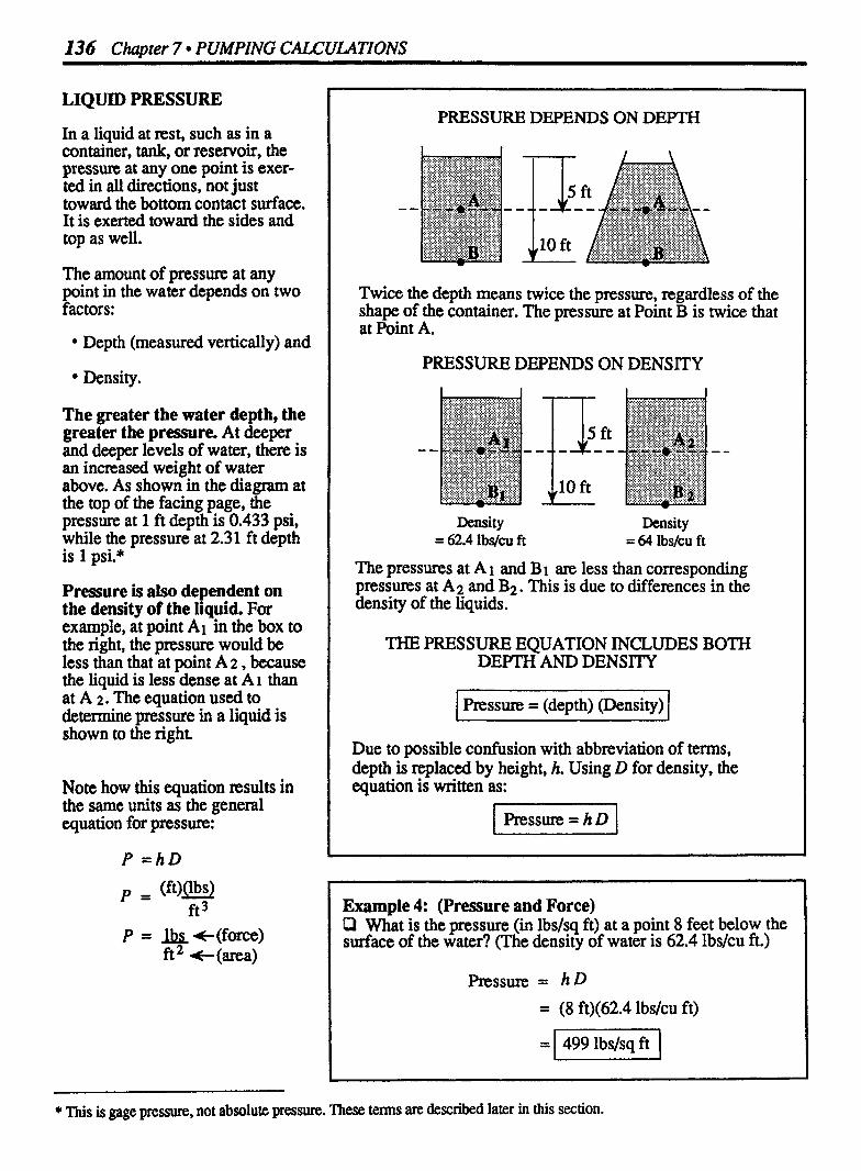
136 Chapter 7 PUMPING CALCULATIONS
LIQUID PRESSURE
In a liquid at rest, such as in a container, tank, or reservoir, the pressure at any one point is exer- ted in all directions, not just toward the bottom contact surface. It is exerted toward the sides and top as well.
The amount of pressure at any point in the water depends on two factors:
Depth (measured vertically) and
Density.
The greater the water depth, the greater the pressure. At deeper and deeper levels of water, there is an increased weight of water above. As shown in the diagram at the top of the facing page, the pressure at 1 ft depth is 0.433 psi, while the pressure at 2.31 ft depth is 1 psi.*
Pressure is also dependent on the density of the liquid. For example, at point A1 in the box to the right, the pressure would be less than that at point A 2 , because the liquid is less dense at A 1 than at A 2. The equation used to determine pressure in a liquid is shown to the right
Note how this equation results in the same units as the general equation for pressure:
P = Ibp t (force) ft2 +(area)
PRESSURE DEPENDS ON DEPTH
Twice the depth means twice the pressure, regardless of the shape of the container. The pressure at Point B is twice that at Point A.
PRESSURE DEPENDS ON DENSITY
Density Density = 62.4 lbs/cu ft = 64 lbs/cu ft
The pressures at A 1 and B1 are less than corresponding pressures at A2 and B2. This is due to differences in the density of the liquids.
THE PRESSURE EQUATION INCLUDES BOTH DEPTH AND DENSITY
1 Pressure = (depth) (Density) l Due to possible confusion with abbreviation of terns, depth is replaced by height, h. Using D for density, the equation is written as:
[GLzq
Example 4: (Pressure and Force) P What is the pressure (in lbsjsq ft) at a point 8 feet below the surface of the water? (The density of water is 62.4 lbsjcu R)
Pressure = h D
= (8 ft)(62.4 lbslcu ft)
* This is gage pressure, not absolute pressure. These terms are described later in this section.

Pressure and Force 137
PRESSURE AND PSI 1 ft = 0.433 psi 1 psi = 2.31 ft
area
The weight bearing down on each square inch of area is about a half pound (0.433 lbs)
area
for each fooiof depth. At a depth of 2.3 1 ft, there is one pound of weight bearing down on each square inch of area.
I Example 5: (Pressure and Force) Cl What is the pressure (in psi) at a point 12 ft below the surface? Using the equation 1 psi = 2.31 ft, draw the box diagram:
I Converting from feet to psi, the move is from a larger box to a smaller box. Division by 2.3 1 is therefore indicated:
Example 6: (Pressure and Force) P At a point 3 ft below the liquid surface, what is the pressure in psi? (The specific gravity of the liquid is 0.95.)
First calculate psi as usual, using the box diagram:
Division is indicated:
The specific gravity may now be taken into account. A specific gravity less than that of water will result in a smaller psi reading for the same water depth:
Pressure at Different = @si)(specific gravity) Sp. Grav.
= (1.3 psi)(O.95)
USING PSI AND FT
Since the density of water is a given in most water and wastewater calculations, the P = hD equation can be shortened. The pressure at 1 ft depth is always 62.4 lbs/sq ft or 0.433 lbs/sq in.*
W hen the " box methodN of conversion is used,** however, both numbers of the equation must be greater than one. The equation shown above may be easily converted to the desired form by dividing both sides of the equation by 0.433, as follows:
1 ft - - W psi 0.433 W WEE3
1 2.31 ft = l psi I Now rearrange the equation so the one is on the left side of the equation:
11 psi = 2.31 ft I This equation can be used in all conversions between feet and psi. It is recommended that this equation be memorized. Example 5 illustrates a conversion between feet and psi.
PRESSURE AND SPECIFIC GRAVITY
Specific gravity can be used to determine pres sum within liquids of different densities. First, calculate the pressure in psi using the equation given above (1 psi = 2.3 1 ft). Then multiply the psi result by the specific gravity of the liquid. Example 6 illustrates this calculation.
* To verify this P = (1 ft)(62.4 lbs/cu ft) = 62.4 lbs/sq ft. To convert to lbs/sq in., divide by 144 sq in./sq ft. For a discussion of square terms conversions, refer to Chapter 8 in Basic Math Concepts.
** The box method of conversions is described in Chapter 8 in Basic Math Concepts.

I38 Chapter 7 PUMPING CALCULATIONS
TOTAL FORCE
The total force of water against the side or bottom of a tank or wall is determined by multiplying the pressure at that depth tims the entire =a:
I Total Force = (Pressure)(Area) I If the pressure is given as lbs/sq ft, the area must be expressed as square feet. And if the pressure is given in lbs/sq in., the area must be expressed as square inches.
Total = (Pressure)(Area) Force lbdsqft sq ft
Total = (Ressure)(Area) Force lbs/sq in. sq in.
Calculating the total force against the bottom of a tank is a straight - forward calculation-simpl y determine the pressure at the bottom of the tank (based on the vertical distance beneath the surface of the water) and multiply this pressure by the area of the bottom.
Calculating the total force against the side of a tank is a little different-which pressure value should be used? 'Ibe pressure at the water surface is zero*, and the pressures increase toward the bottom of the tank. The pressure to be used in these calculations is the average pressure. The average pressure occurs at half of the water depth, or what might be termed the average depth. Average depth may be determined as follows:
Average - Total Depth, ft Depth, ft - 2
Example 8 illustrates this type of calculation.
TOTAL FORCE AGAINST THE BOTTOM OF A TANK
Total = (Pressure) (Area) Force lbslsq ft sq ft
TOTAL FORCE AGAINST THE SIDE OF A TANK
f 3 ft
Total = (Pressure at Average) (Total Area) I Force Depth, lbs/sq ft sq ft
Example 7: (Pressure and Force) P What is the total force against the bottom of a tank 30 ft long and 10 ft wide? The water depth is 8 ft.
First, calculate the pressure at the bottom of the tank. At 8 ft depth, the pressure is:
ft = 3.46 psi 2.31 ftlpsi
Then calculate total force. Since pressure is given in psi, the dimensions must be reported in inches (30 ft X 12 in/ft = 360 in.; 10 ft X 12 in./ft = 120 in.)
= (3.46 psi) (360 in.) (120 in.)
* Referring to gage pressure. Absolute and gage pressures are described later in this section.

Pressure and Force 139
Example 8: (Pressure and Force) Q What is the total force exerted on the side of a tank if the tank is 16 ft wide and the water depth is 12 ft?
Since the water depth is 12 ft, the halfway point (or average water depth) is 6 ft. To calculate total force, the pressure at the average depth must be calculated. The pressure at a depth of 1 ft = 62.4 lbs/sq ft, so the pressure at 6 ft would be:
(6)(62.4 lbslsq ft) = 374 lbslsq ft average pressure
Now the total force can be calculated:
Total = messure at Average) (Total Area) Force Depth, lbs/sq ft sq ft
= (374 lbs/sq ft) (12 ft) (16 ft)
THE CENTER OF FORCE IS LOCATED ALONG A LINE 213 FROM THE SURFACE
Triangular Load Front View of Wall (Side View of Wall)
In Example 8, the total force against the wall is 71,808 lbs. Where is the center of force located?
Center = (2J (Depth of) 0fForce 3 Water
= pJ (12 ft) 3
An equation sometimes given for the total force on the side of a tank is:
F = (31.2) (H 2, (L),
where F = force in lbs, H = head in ft, and L = length of wall in ft. This equation is simply an abbreviation of the typical total force equation, as shown below: (note the water depth is written as H, ft of head)
Total Force, = (Pressure)(Area) lbs lbslsq ft sq ft
i n = (Aver.)@en.) (Area)
height
TOTAL FORCE VS CENTER OF FORCE
Although the total force on a side wall is calculated using the average depth (or average pressure, since these are related), the center of force is not located at the halfway line-it is located along a line two-thirds of the way down from the water surface.
This is because the pressure against the wall increases with depth (forming what is called a "triangular load"). As shown in the diagram to the left, more of the force against the wall is located nearer the bottom. To calculate the center of force on a wall, simply multiply the water depth by 2l3:
Center = (2J (Depth of) L r c e 3 Water
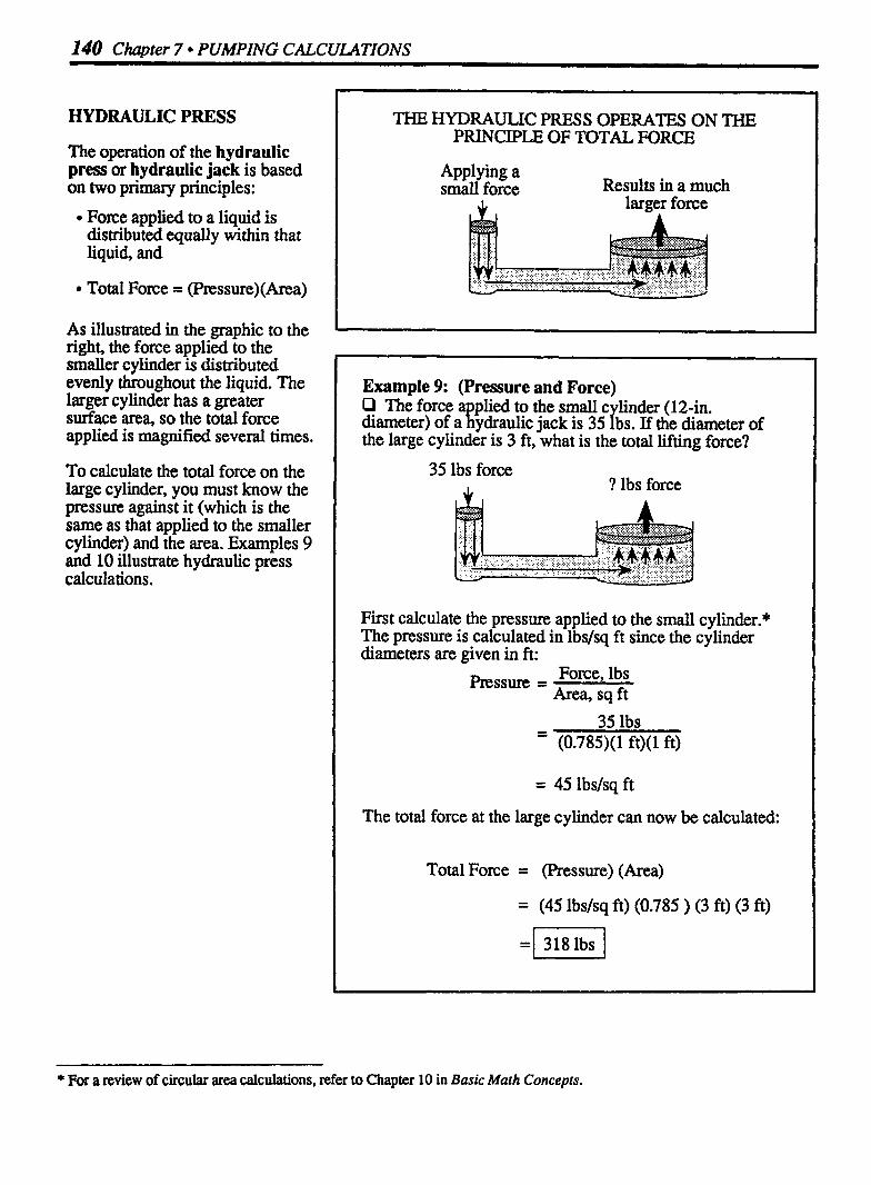
140 Chapter 7 PUMPING CALCULATIONS
HYDRAULIC PRESS
The operation of the hydraulic press or hydraulic jack is based on two primary principles:
Force applied to a liquid is distributed equally within that liquid, and
Total Force = (Pressure)(Area)
As illustrated in the graphic to the right, the force applied to the smaller cylinder is distributed evenly throughout the liquid. The larger cylinder has a greater surface area, so the total force applied is magnified several times.
To calculate the total force on the large cylinder, you must know the pressure against it (which is the same as that applied to the smaller cylinder) and the area. Examples 9 and 10 illustrate hydraulic press calculations.
THE HYDRAULIC PRESS OPERATES ON THE PRINCIPLE OF TOTAL FORCE
Results in - a much larger force
Example 9: (Pressure and Force) P The force a plied to the small c linder (12-in. K diameter) of a ydraulic jack is 35 Y bs. If the diameter of the large cylinder is 3 ft, what is the total lifting force?
35 lbs force I ? lbs force
First calculate the pressure applied to the small cylinder.* The pressure is calculated in lbs/sq ft since the cylinder diameters are given in ft:
Pressure = Force, lbs Area, sq ft
- 35 lbs - (0.785)(1 ft)(l ft)
= 45 lbslsq ft
The total force at the large cylinder can now be calculated:
Total Force = (Pressure) (Area)
= (45 lbs/sq ft) (0.785 ) (3 ft) (3 ft)
* For a review of circular area calculations, refer to Chapter 10 in Basic Math Concepts.

Pressure and Force 141
Example 10: (Pressure and Force) Q The force applied to the small cylinder of a hydraulic 'ack is 50 lbs. The diameter of the small cylinder is 18 mches. Ifthe diameter of the large cylinder is 40 inches, what is the total lifting force?
50 lbs 1 ? lbs
First calculate the pressure applied to the small cylinder. Since the diameters of the cylinders are given in inches, the pressure will be calculated as lbs/sq in.:
Pressm = Force, lbs Area, sq in.
- 50 lbs - (0.785)(18 in.)(18 in.)
= 0.2 lbslsq in.
The same pressure is transmitted to the larger cylinder. The total force at the large cylinder is calculated as:
= (0.2 lbsl(0.785) (40 in.) (40 in.) sq in.
Example 11: (Pressure and Force) Q A ga e reading is 25 psi. What is the absolute pressure at the gage 5 (Assume sea level atmospheric pressure.)
Absolute = Gage Pressure + Atmospheric Pressure, psi psi Pressure, psi
= 25 psi + 14.7 psi
= 139.7 psi I
GAGE VS. ABSOLUTE PRESSURES
When water pressures are measured in a tank or pipeline, they are measured by gages. These measurements are therefore called gage pressures. Gage pressures do not include all the pressures acting in the tank or pipeline-they do not include atmospheric pressure.
Atmospheric pressure is generally not considered in water and wastewater calculations, because atmospheric pressure is exerted both inside and outside the tank or pipeline. At sea level, the atmospheric pressure is 14.7 psi. The name given to the total pressure, including both gage and atmospheric pressures, is absolute pressure. Absolute pressure is calculated by adding the gage pressure and atmospheric pressure:
Absolute Gage Atmos. Press., = Press. + Press.,
psi psi psi
Example 11 illustrates a calculation involving gage and absolute pressures.

142 ChaDter 7 PUMPING CALCULATIONS
7.3 HEAD AND HEAD LOSS
HEAD TERMINOLOGY
When describing the various types of head against which a pump must operate, several different terms may be used, depending on the side of the pump and whether or not the pump is operating.
SUCTION AND DISCHARGE HEADS
The terms suction and discharge indicate two different sides of the pump. As shown in the diagram to the right, the suction side of a pump is the inlet or low pressure side of the pump. The discharge side of a pump is the outlet or high pressure side of the pump.
Heads measured on the suction side of a pump are called suction heads. Heads measured on the discharge side of a pump are called discharge heads.
--
THE TWO SIDES OF A PUMP
SUrnON SIDE OF
THE PUMP
pump Centerline, 6
DISCHARGE SIDE OF
THE PUMP
SUCTION HEAD, SUCTION LET, AND DISCHARGE HEAD
When the water feeding the pump is above the pump, this is called a suction head:
When the water feeding the pump is below the pump, this is called a suction lif't:

Pressure and Force I43
TOTAL STATIC HEAD IS THE VERTICAL DISTANCE BETWEEN THE
TWO FREE WATER SURFACES
When the two water surfaces are located above the pump, the static suction head offsets part of the static discharge head. The total static head is therefore the difference in height between the two heads:
Totalstatic = Higher Lower Head, ft Elevation, ft Elevation, ft
I I (stktic) (sktic)
Discharge Suction Head Head
When the water surface on the suction side of the pump is below the pump centerline, there is no offsetting head on the suction side. The total static head is therefore the sum of the two heads:
. . .. l Suction L .. . . . . . . ,:;a .. . 9 ._ . . , .... , .. . ::. .. ... ..,. -. Li.
v . . . . . . . . . . . . . . ... . . . .:: . . . . . . . . . _. . . . ., ._. . . . . . . ... .... ... . . . . . . . . . . . . . . . . . -. . . . ... :. . : : ' . : ... ..... .. .... .. .... . . ... . . . . , . ,. ,. . . . . . . . . . ... . . .,.. .. . :.. ..:._ ,._. ..... , _. . ., . ...: ._ . . ... . . . .. .. ... . . . . . . .. .. .... . . . .;., .(. . ..._.. ... .. . ... . .. . . . .. ... , . . . . _ . ~ . . ' ..
Distance p;a;;aic = Height + Above Pump Below Pump Centerline, ft Centerline, ft
STATIC HEAD
The total head against which a pump must operate is determined princi- pally by two calculations:
Total static head, and
Friction and minor head losses
Head measurements taken on either side of the pump when the pump is off are called static heads. Both the static suction head and static discharge head are considered when determining the total static head, as illustrated in the diagrams to the left.
In simplified terms, however, total static head is a measure of the ver- tical distance between the two water surface elevations. It can be mea- sured using elevations, vertical measurements, or gage pressures.

I44 Chapter 7 PUMPING CALCULATIONS
TOTAL DYNAMIC HEAD CTDW
In addition to static head, the pump must work against friction and minor head losses. These are head losses resulting from friction as the water rubs against the pipeline and from friction and changes in direction as the water moves through valves and orifices.
For example, if the water is to be lifted 50 ft from Point A to Point B (as shown in the diagram to the right) and head losses are equal to 5 ft, the pump must produce a total of 55 ft of head to lift the water fiom Point A to Point B.
The total head against which the pump must operate is called the total dynamic head (TDH).
Total Total Head Dynamic = Static + Losses, Head, ft Head, ft ft
DYNAMIC HEAD IS THE STATIC HEAD PLUS FRICTION AND MINOR HEAD LOSSES
Additional head required to compensate for friction and minor 1 -
Example 1: (Head and Head Loss) O The elevation of two water surfaces are Oven below. If the
dynamic head (in ft)? l? friction and minor head losses equal 9 ft, W at is the total
Total Dynamic , Total Static + Head Losses Head, ft Head, ft ft
= (742 ft - 620 ft) + 9 ft
= I 131 ft TDH 1

Head and Head Loss 145
Example 2: (Head and Head Loss) P he ump inlet and outlet age readings are given below. &mp is off*) If the fnction an 8 minor head losses are equal to 12 ft, what is the total dynamic head (in ft)?
First calculate the static head in psi, then convert head in psi to head in ft. The static head is the difference in inlet and outlet pump pressures: 150 psi - 90 psi = 60 psi.
Next, convert 60 psi to ft*: (1 psi = 2.3 1 ft)
Then calculate the total dynamic head:
(60 psi) (2.3 1 ftfpsi) =
TDH = Static Head + Head Losses
= 139 ft + 12 ft
139 ft Static Head
Example 3: (Head and Head Loss) Ll Readin S taken from the inlet and outlet pressure gages of a k pump whi e it is in operation are as follows: 87 psi and 143 psi, respectively. What is the TDH, in ft?
The difference in pressure readings is 143 psi - 87 psi = 56 psi. Convert this difference in psi to ft:
(56 psi)(2.31 ft/psi) = 129 ft TDH c 3
If the pressure is expressed in psi, it can be converted to feet, if desired* Example 2 illustrates such a calculation.
When a pump is operating, it operates against the heads and head losses described above. Inlet and outlet gage pressures taken when the pump is operating, therefore, are a good estimate of the total dynamic head. Example 3 illustrates this calculation*
I I
* Refer to Section 7.2 for a discussion of psi and ft conversions.

146 Chapter 7 PUMPING CALCULATIONS
FRICTION HEAD LOSS
Friction head losses within a pipeline depend on several factors:
Velocity or rate of flow,
Diameter of pipe,
Length of pipe, and
Pipe roughness.
Friction losses are determined by using tables such as that shown on the facing page. Values on this table are calculated using the Hazen-Williams formula, which includes a roughness coefficient, C. The smoother the pipe, the higher the C-value.
The table on the facing page is bsised on a C-value of 100. To determine friction loss:
1. Enter the table at the known pipe diameter. (Diameters are shown across the top of the table.)
2. Follow the column down until it is opposite the given flow rate, mm*
3. Read the corresponding friction loss. The loss is given in feet and represents the friction loss for every 100-ft section of pipe.
4. Calculate the total friction loss for the pipeline by multiplying the friction loss by the number of 100-ft segments of pipe.
A wide variety of pipes in use today have C-values from 130 to 140 and greater. Reference books are available that include fiiction loss tables for various other C-values.
Example 4: (Head and Head Loss) P A 6-inch diameter pipe has a C-value of 100. When the flow rate is 240 gpm, what is the fiiction loss for a 2000-ft length of pipe?
Enter the top column at "6-in. Pipe". Come down the column to the entry across from 240 gpm. The friction loss shown is 0.87 ft per 100-ft segments.
2 ~ . - - , There are 20 100-ft
? segments of pipe
hundreds place decimal
Total Friction = (0.87 fi)(20 segments) Loss, ft of 100-ft
Example 5: (Head and Head Loss) 0 Flow through an &inch pipeline is 1300 gpm. The C-value is 100. What is the friction loss through a 3500-ft section of pipe ?
Enter the table at the 8-inch diameter heading and follow the column down until you are across from the 1300 gpm value. The friction loss indicated is 4.85 ft per 100-ft segment of pipeline.
3500.- There are 35 100-ft
.r segments of pipe
hundreds place decimal
Total Friction = (4.85)(35 segments) Loss, ft of 100-ft
Note that these tables do not apply when pumping sludges.

Head and Head Loss 147
FRICTION LOSS IN FEET PER 100-FT LENGTH OF PIPE (Based on Williams & Hazen Formula Using C = 100)
' b in . ~ i p . %.in . Pipe lain . ~ i p e lllr.in . Pipe llh-in . ~ l p . ( 2.in . P i p 2lkin . PI^^ 3.1". Pipe 4 4 1 . pipe 54n . PI p. 6-nr Plp i US Vat . L o u V . LOW V01 . Loss Vel . Loss Vat . Loss Vd . Loss Vat . W vet . ~ 0 - V d . Lou Vol . Lou ~d . bn US
011 H per in fl W in ft par in ft prr in H per in H per in tt per in ft mr In i t per in ft por in tt per In 9.1 permilr 8OC fi m fi WC ft wc fi we ft fi #C H R $ 8 ~ ft 68C ft WC ft mrdn -- -
2 2.10 7.4 1.20 1.9 .............................................................................................................................. 2 4.21 21.0 2.41 7.0 1.49 2.14 . 86 S7 .W ' : 6.31 7 . 3.61 14.7 2 . a 4.55 1.29 1.m .W
8 8.42 98.0 4.11 25.0 2.W 1.8 1.72 203 1.28 10 10.52 147.0 6.02 38.0 3.12 11.7 2.14 3.05 1.57
12 ................ 7.22 53.0 4.46 16.4 2.57 4.3 1.89 S 15 ................ 9.02 60.0 5.60 25.0 3.21 6.5 2.36
18 ................ 10.84 108.2 6.69 35.0 3.06 9.1 2.83 20 ................ 12.03 136.0 7 . U 42.0 4.29 11.1 3.15 ................................ 25 9.30 0 5.36 16.6 3.80 30 ................................ 11.15 0 6.43 23.0 4.72 35 13.02 110.0 7.51 31.2 5.51 ................................
. 40 ................................ 14.88 152.0 8.56 40.0 6.30 , 45 9.65 50.0 7.00 ................................................ 50 10.72 60.0 7.87 ................................................ 55 11.78 72.0 8.66 ................................................ 60 .............................................. 12.87 85.0 9.44 ................................................ 65 13.92 99.7 10.23
70 ................................................ 15.01 113.0 11.02 75 16.06 129.0 11.80 ................................................ W ) .............................................. 17.16 145.0 12.59 a 18.21 163.8 13.38 ................................................ 90 ................................................ 19.30 180.0 14.71 95 ............................................................... 14.95
100 ............................................................ 15.74 ............................................... 1 l 0 17.31
120 1 8 " P i p e 1 ............................................... 18.89 ............................................... 130 20.46 140 . 90 .m ............................................... 22.04 150 . 96
160 1.02 170 1.00 180 1.15 190 1.21 200 1.28 220 1.40
240 1.53 260 1.66 280 1.79 300 1.91 320 2.05 340 2.18 1 pp - $
. l0 .............................................................
. l 1 ..........................................................
. 13 .............................................
. 14 .f 10" Pipe ............................................. ............................................. ............................................ ............................................
.............................................
.............................................
.............................................
..........................................
Reprinted from Basic Science Concepts and Applications. by permission . Copyright O 1980. American Water Works Association .

148 Chapter 7 PUMPING CALCULATIONS
MINOR HEAD LOSS
Minor head losses are a result of water moving through valves and orifices, causing rapid changes in velocity and direction of flow.
These losses may be estimated using the nomograph* given on the facing page.
To read the nomograph, follow these steps:
1. Place one end of a straightedge at the known pipe diameter on the right scale.
2. Align the other end of the straight edge with the point designated for the desired fitting or orifice on the left scale.
3. Draw a line fiom the left scale to the right scale and read the head loss value on the middle scale.
The values given in the table represent equivalent length of straight pipe. These values are to be added to actual pipe length for calculation of fiction losses, described on the previous page.
Minor losses are normally just that-minor, when compared to friction loss values. However, the smaller the runs of pipe, the more significant are these minor head losses.
Examples 6 and 7 illustrate the use of the nomograph in determining minor friction losses.
Example 6: (Head and Head Loss) O Determine the "equivalent length of p ip" for a flow through a swing check valve, fully open, if the diameter of the pipe is 6 inches.
Align one end of the straightedge with the 6-inch (nominal diameter) mark on the left side of the scale shown to the right.
Align the other end of the straightedge with the point indicated for the "Swing Check Valve, Fully Open."
Draw a line from the left scale to the right scale.
The "equivalent length" value can be =ad on the middle scale:
1 40 ft equivalent length of pipe I
Example 7: (Head and Head Loss) P What is the head loss through a gate valve (In closed) for a 10-inch diameter pipeline?
Align one end of the straightedge with 10-inches (nominal diameter) on the scale to the right.
Align the other end of the straightedge with the point corresponding with "Gate Valve-112 Closed on the scale to the left.
Draw a line between the two outside scales and read the head loss value from the middle scale. The approximate reading is:
1 170 ft equivalent length of pipe I
* For a review of reading nomographs, refer to Chapter 12 in Basic Math Concepts.
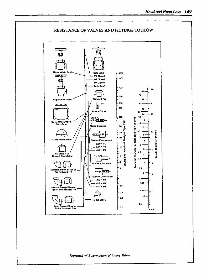
Head and Head h s s 149
Globe Valve. Open
Angle Vdve, Open
Swina Check Valve. F;II~ Open
Closo Return Bend '/
Standard T r e Through Side Outlet
Standard Elbow or run of Tee Reduced 1/2
Medium Sweep Elbow or - Run of Tee Reduced 1/4
Long Sweep Elbow or - Run of Standard fee
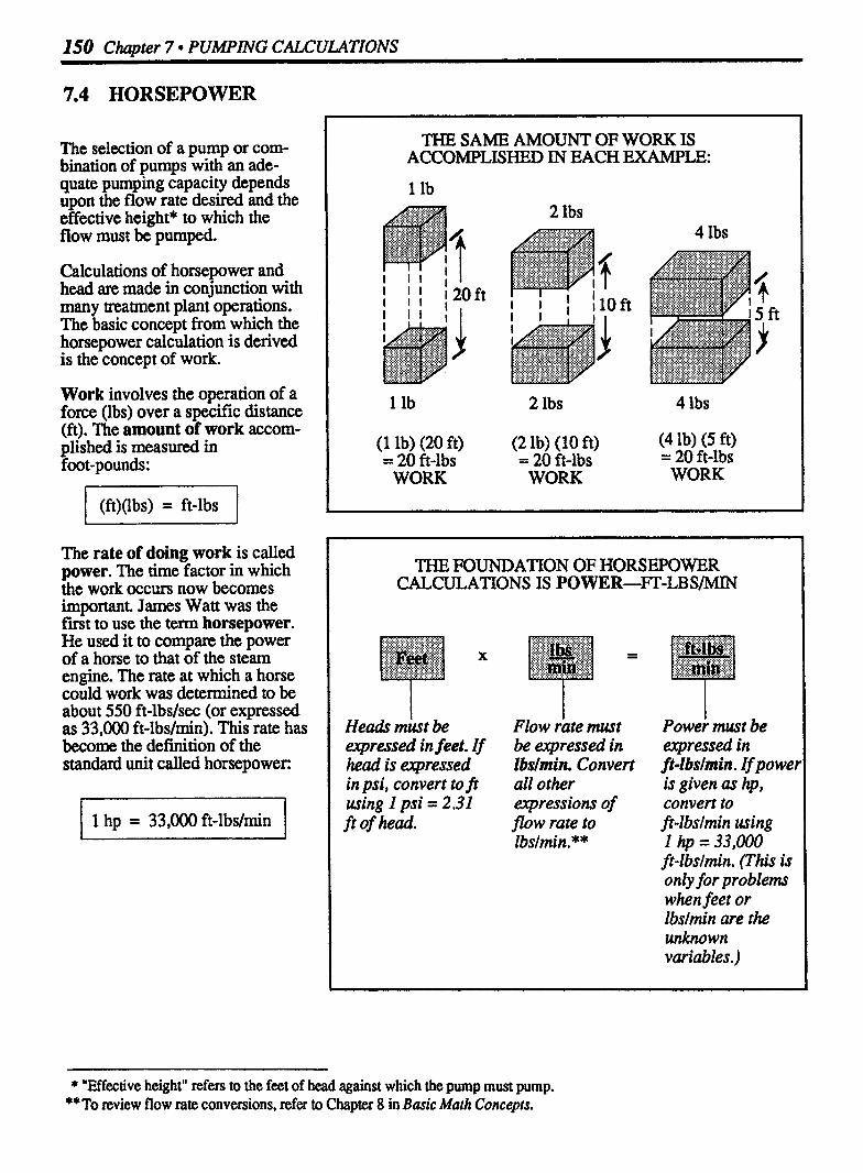
150 Cha~ter 7 PUMPING CALCULATIONS
7.4 HORSEPOWER
The selection of a pump or com- bination of pumps with an ade- quate pumping capacity depends upon the flow rate desired and the effective height* to which the flow must be pumped.
Calculations of horsepower and head are made in conjunction with many treatment plant operations. The basic concept from which the horsepower calculation is derived is the concept of work.
Work involves the operation of a force (lbs) over a specific distance (fi). The amount of work accom- plished is measured in foot-pounds:
/ (ft)(lbs) = ft-lbs 1 The rate of doing work is called power. The time factor in which h e work occurs now becomes important. James Watt was the fmt to use the term horsepower. He used it to compare the power of a horse to that of the steam engine. The rate at which a horse could work was determined to be about 550 ft-lbs/sec (or expressed as 33,000 ft-lbs/min). This rate has become the definition of the standard unit called horsepower:
THE SAME AMOUNT OF WORK IS ACCOMPLISHED IN EACH EXAMPLE:
2 lbs 4 Ibs
I I I I I I I 120ft l I I 1
1 lb 2 Ibs 4 lbs
( l lb) (20 ft) (2 lb) (10 ft) (4 lb) (5 ft) = 20 fi-lbs = 20 ft-lbs = 20 ft-lbs WORK WORK WORK
THE FOUNDATION OF HORSEPOWER CALCULATIONS IS POWER---FT-LB S/MIN
Headr &t be expressed in feet. If head is expressed in psi, convert to fr using I psi = 2.31 ft of head.
Flow rate must be expressed in lbslmin. Convert all other expressions of flow rate to lbslmin. * *
~ o w e i must be expressed in ft-lbslmin. r f powe~ is given as hp, convert to ft-lbslmin using I hp = 33,000 ft-lbslmin. (This is only for problems when feet or lbslmin are the unknown variables.)
* "Effective height" refers to the feet of head against which the pump must pump. **To review flow rate conversions, refer to Chapter 8 in Basic Math Concepts.

Horsepower I51
Example 1: (Horsepower) Cl A ump must pump 2000 m against a total head of 20 ft. K F What orsepower is required or this work?
First calculate ft - lbs/min required:
2000 gpm must be converted to
lbsimin: (2000 gpm)(8.34) = 16,680
lbs/gal lbs/m.n I
9 (20 ft)
+ X (16,680 lbslmin) =
ft-lbs/min
Then convert ft-lbslmin to hp:
333,600 ft-lbslmin 33,000 ft-lbs/min/hp
Example 2: (Horsepower) P A flow of 8 MGD must be pumped against a total dynamic head (TDH) of 25 ft. What horsepower is required for this work?
(25 ft)
8,000,000 gpd mwt be converted to lbslmin:
Then convert ft-lbdmin to hp: I I
CALCULATING HORSEPOWER
When calculating honepower requirements:
1. Determine the ft-lbslmin power required:
2. Once ft-lbslmin power has been calculated, horsepower can be determined using the equation 1 hp = 33,000 ft-lbdmin.
AN ALTERNATE EQUATION
An equation frequently given for horsepower calculations is:
[P-- (flow rate) (total- head) m
whp = ft 3960
This equation is derived from the horsepower equation described above:
ft-lbs/mi.n hp 33,000 ft-lbs/min/hp
It is then adjusted to reflect gprn flow rate, rather than lbs/min flow rate. The advantage of this equation is that gpm may be used directly, without conversions. The disadvantage is that it is somewhat "cut off from its roots":-the concept of power, ft-lbslmin. Because of this, there is often a lack in flexible application of thc equation. It tends to become an equation memorized but not fully understood.
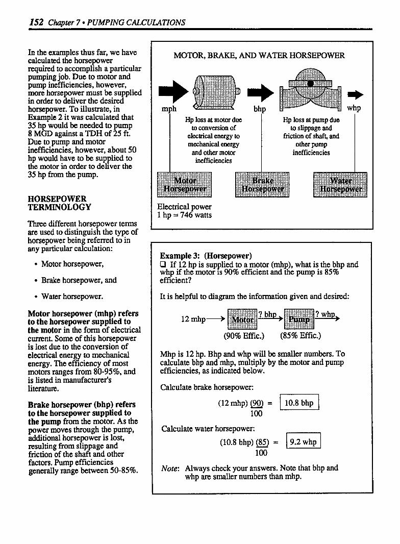
152 Chapter 7 PUMPING CtUCULATIONS
In the examples thus far, we have calculated the horsepower required to accomplish a particular pumping job. Due to motor and pump inefficiencies, however, more horsepower must be supplied in order to deliver the desired horsepower. To illustrate, in Example 2 it was calculated that 35 hp would be needed to pump 8 MGD against a TDH of 25 ft. Due to pump and motor inefficiencies, however, about 50 hp would have to be supplied to the motor in order to deliver the 35 hp from the pump.
HORSEPOWER TERMINOLOGY
Three different horsepower terns are used to distinguish the type of horsepower being referred to in any particular calculation:
Motor horsepower,
Brake horsepower, and
Water horsepower.
Motor horsepower (mhp) refers to the horsepower supplied to the motor in the form of electrical current. Some of this horsepower is lost due to the conversion of electrical energy to mechanical energy. The efficiency of most motors ranges from 80-9596, and is listed in manufacturer's literature.
Brake horsepower (bhp) refers to the horsepower supplied to the pump from the motor. As the power moves through the pump, additional horsepower is lost, resulting from slippage and friction of the shaft and other factors. Pump efficiencies generally range between 50-8596.
MOTOR, BRAKE, AND WATER HORSEPOWER
Hp loss at motor due to conversion of
electrical energy to mechanical energy and other motor inefficiencies
Hp loss at pump due to slippage and
friction of shaft, and other pump
inefficiencies
Electrical power 1 hp = 746 watts
Example 3: (Horsepower) P If 12 hp is supplied to a motor (mhp), what is the bhp and whp if the motor is 90% efficient and the pump is 85% efficient?
It is helpful to diagram the information given and desired:
(90% Effic.) (85% Effic.)
~p is 12 hp. Bhp and whp will be smaller numbers. To lculate bhp and rnhp, multiply by the motor and pump iciencies, as indicated below.
Calculate brake horsepower:
(12 mhp) (90) = I 10.8 bhp I Calculate water horsepower:
(10.8 bhp) (9 = 1 9.2 whp I loo
Note: Always check your answers. Note that bhp and whp are smaller numbers than mhp.

Horsepower 153
Example 4: (Horsepower) O 40 h is supplied to a motor. How many horsepower will be avai P able for actual pumping loads, if the motor is 92% efficient and the pump is 85% efficient?
In this problem, the unknown hp is w h ~ ("available for actual pumping loads "). First diagram the problem:
(92% Effic.) (85% Effic.)
To calculate whp, multiply mhp by both the motor and pump efficiencies:
(40 mhp) (92) (85) = 1 31.3 whp I -- loo loo
Example 5: (Horsepower) O A total of 28 hp is required for a particular pumping application. If the pump efficiency is 75% and the motor efficiency is 85%, what horsepower must be supplied to the motor?
In this problem, the unknown tern is mhp. Remember that the answer must be a larger number than the whp (28 hp).
First diagram the information in the problem:
(85% Effic.) (75% Effic.)
To calculate mhp, divide by pump and motor efficiencies:
Note that the mhp calculated is in fact a larger number than whp.
Water horsepower (whp) refers to the actual horsepower available to pump the water. Examples 1 and 2 in this section were actually calculations of water horsepower.
When making calculations of motor, brake, and water horsepower, it is important to remember that motor horsepower will be the largest number, brake horsepower next largest, followed by water horsepower. Knowing the relative sizes of these terns will help you know if your answers are reasonable.
The conversion between horsepower tenns can be calculated as follows:
When converting from a smaller term to a larger term* (such as whp to bhp, bhp to mhp, or whp to mhp), divide by the efficiency of the pump or motor:**
Brake hp = Water hp Pump Effic.
Motor hp = Brake hp Motor Effic.
Motor - Water hp
hp < ~ o t o r Effic.)(Pump EEC.)
When converting from a larger term to a smaller tern (such as mhp to bhp, bhp to whp, or mhp to whp), multiply by the efficiency of the pump or motor: **
Brake hp = (Motor)(Motor) hp Efftc.
Water hp = (Brake)Wp) hp Effic.
Water hp = (Motor)(Motor)(Pump) hp Effic. Effic.
* Normally, when converting from a smaller term to a larger term, multiplication is indicated. However, that is only true when multiplying by a number one. When a number less than one (such as pump or motor efficiency) is multiplied times a number . the answer is a smaller number; when a number less than one is used to divide a number, the resulting answer is larger number.
** Efficiency is written as 401100. For example 80% efficiency is written as 801100. This can be simplified as 0.80.

154 Chapter 7 PUMPING CALCULATIONS
HORSEPOWER AND SPECIFIC GRAVITY
In Examples 1-5, the horsepower calculations were based on pumping water. If another liquid is to be pumped, the specific gravity* of the liquid must be conside~d.
The specific gravity of a liquid is an indication of its density, or generally its weight, compared to that of water.
To account for differences in specific gravity, include the specific gravity factor when calculating ft-lbs/min pumping requirements:
I (ft)(lbs/min)(sp. gr.) = ft-W& for different
I liquid I Example 6 illustrates such a calculation.
MHP AND KILOWATT REQUIREMENTS
Motor horsepower requirements can be converted to watts and then kilowatts requirements using the following equation: * *
I 1 hp = 746 watts (
Once watts requirements are determined, kilowatts are easily determined by a metric system conversion.
Example 6: (Horsepower) Q A pump must ump a ainst a total dynamic head of 50 ft at a flow rate of 13 & gpm. k e liquid to be pumped has a specific gravity of 1.3. What is the water horsepower requirement for this pumping application?
Water horsepower is essentially a calculation of ft-lbs/min. A specific gravity factor must be included in this calculation:
1300 gpm must be converted to lbslmin. The
spec. grav. factor is included in this calculation:
(1300) (8.34) (1.3) = 14,095 gpm lbslgal sp. g. lbs/min
I I (50 ft) X (14,09&bs/min)
ft-lbs/min
Now convert ft-lbs/min to hp:
Example 7: (Horsepower) P The motor horsepower requirement has been calculated to be 35 hp. How many kilowatts electric power does this repre sent?
First calculate the watts required using the equation 1 hp = 746 watts. The box method of conversions may be used:
Multiplication by 746 is indicated:
(35 hp) (746 wattshp) = 26,110 watts
26,110 watts Then: loo0 watts/kW
* Specific gravity is discussed in Section 7.1 of this chapter. ** This equation is preferred to the equation 1 hp = 0.746 kW, since the box method of conversion works only if
both numbers are greater than one. Refer to Chapter 8 in Baric Math Concepts.

Horsepower 155
Example 8: (Horsepower) uired for a pumping application. If the cost of
power 22dfisrs% is 0.052 /km, and the pump is in operation 24 hrs/day, what is the daily pump cost?
To calculate kWh pump operation, you must know the kW power requirements of the motor and hours of operation. First convert 22 mhp to kW: (1 hp = 746 watts)
(22 mhp) (746 watts&) = 16,412 watts
The kWh of power consumption can now be determine'
Now complete the cost calculation:
Example 9: (Horsepower) D The motor horsepower requirement has been calculated to be 50 mhp. During the week, the pump is in operation a total of 148 hours. Using a power cost of $0.09439/lcWh, what would be the power cost that week f a the pumping?
First convert 50 mhp to kW so that kWh can be calculate& (1 hp = 746 watts)
(50 mhp) (746 wattshp) = 37,300 watts
Next calculate k W ' of power consumed:
(37.3 kW) (148 hrs) = (5520 kWh 1 Then powers costs may be calculated:
(5520 kVVh/wk) ($0.09439) = $521 -03 k m ( costfor 1 the week
PUMPING COST CALCULATIONS
Pumps costs are determined on the basis of two primary considerations:
Kilowatt-hours of pump operation, and
Power cost per kilowatt-hour.
Kilowatt -hours of pump operation are determined by multiplying power drawn by the pump (kW) by the hours of operation (hrs):
Once the kilowatt-hours of power use has been determined, then determine the cost of that power use using the cost factor:
(kWh) (Cost/kWh) = Total Power use Cost
Examples 8 and 9 are pumping cost calculations.

156 Chapter 7 PUMPING CALCULATIONS
7.5 PUMP CAPACITY
PUMP CAPACITY TESTING
Pump capacity may be determined by timing the pumping into or out of a tank of known size. Assuming water is not entering or leaving from any some other than the pump being tested, then-
* When pumping into a tank the rise in water level will correspond with the pumping rate.
When pumping out of a tank, the drop in water level will cornspond with the pumping rate.
To calculate the pumping capacity or rate, determine the gallons rise or fall and divide by the time of the pump test:
Pumping = gal rise or fall Rate, gpm minutes of test
(In expanded form for a rectangular tank)
pumping ( I ) (W) (d) (7.48 gaVcu ft) Rate, gpm minutes
WHEN PUMPING INTO AN EMPTY TANK, THE RISE IN WATER LEVEL INDICATES PUMPING RATE
Rise in Level X
WHEN PUMPING FROM A TANK, (WITH INFLUENT VALVE CLOSED) THE DROP XN WATER LEVEL
INDICATES PUMPING RATE
Example 1: (Pump Capacity) P A wet well is 15 ft long and 12 ft wide. The influent valve to the wet well is closed If a pump lowers the water level 1.25 ft during a 5-minute pumping test, what is the gpm pumping rate?
Level
(l5 ft) (12 ft) (1.25 ft) (7.48 gaVcu ft) 5 minutes

Pump Capacities 157
Example 2: (Pump Capacity) O A pump is dischar ed into a 55-gallon barrel. If it takes 35 seconds to fill the arrel, what is the pumping rate in gpm?
%
Since gallons per minute are desired, fmt, convert 35 seconds to minutes,
35 sec 60 sec/min = 0.58 min
then calculate the gpm pumping rate. The equation using tank dimensions is not needed since the gallons pumped (55 gallons) is already known. The general equation may be used:
1 75 gallons "rise"
Pumping - - Rise, gallons Raw, mm Test time, min
- - 55 gallons 0.58 minutes
Example 3: (Pump Capacity) ump is rated at 300 gpm. A pump test is minutes. What is the actual gprn pumping
rate if the wet well is 10 fi long and 8 ft wide-adthe wakr level drops 1.33 ft during the pump test?
Level W Pumping - (Length, ft) (Width, ft) (Drop, ft) (7.48 g d c u ft) Rate, gpm Test time, min
- (10 ft) (8 ft) (1.33 ft) (7.48 gdcu ft) 3 minutes

158 Chuvter 7 PUMPING CALCULATIONS
CAPACITY TESTING WHEN INFLUENT VALVE IS OPEN
In the previous two pages, pump capacity was determined for two conditions:
*Pumping into a tank with known dimensions, and
Pumping from a tank with the influent valve closed.
However, it is possible to determine pumping capacity (or pumping rate) even when the influent valve is open. Examples 4 and 5 illustrate how to calculate pumping rate out of a tank when there is influent entering the tank.
WHEN INFLUENT VALVE IS OPEN INFLUENT FLOW (GPM) MUST BE INCLUDED IN THE CALCULATION
When the water level remains the same, the pumping rate is equal to the influent rate:
Level Remains Constant
Pumping Influent Rate, gpm Flow, gpm
When the water level drops, the pumping rate is greater than the influent rate:
Influent --A f-* Pumping Rate
Pumping = Influent Rate, gpm Flow, gpm + Level, Drop gpm in 1
When the water level rises, the pumping rate is than the influent rate:
Risein Level X
Pumping = Influent - Rise in Rate, gpm Flow, gpm Level, gpm
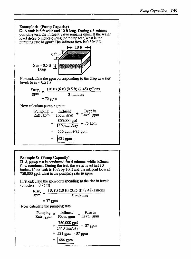
Pump Capacities 159
Example 4: (Pump Capacity) D A tank is 6 ft wide and 10 ft long. During a 3-minute pumping test, the influent valve remains open. If the water level drops 6 inches during the pump test, what is the pumping rate in gpm? The influent flow is 0.8 MGD.
loft +I
First calculate the gpm corresponding to the drop in water level: (6 in = 0.5 ft)
Drop, = (10 ft) (6 ft) (0.5 ft) (7.48) gallons mm 3 minutes
= 75 gprn
Now calculate pumping rate: Pumping = Influent Drop in Rate, gprn Flow, gpm + Level, gpm
= 556gprn+75 gprn
Example 5: (Pump Capacity) Q A pump test is conducted for 5 minutes while influent flow continues. During the test, the water level rises 3 inches. If the tank is 10 ft by 10 ft and the influent flow is 750,000 gpd, what is the pumping rate in gpm?
First calculate the gprn corresponding to the rise in level: (3 inches = 0.25 ft)
Rise, - - (10 ft) (10 ft) (0.25 ft) (7.48) gallons m m 5 minutes
= 37 gprn Now calculate the pumping rate:
Pumping = Influent - Rise in Rate, gprn Flow, gpm Level, gpm
- 750,000 gpd - 37 gprn 1440 midday
= 521 gprn - 37 gpm
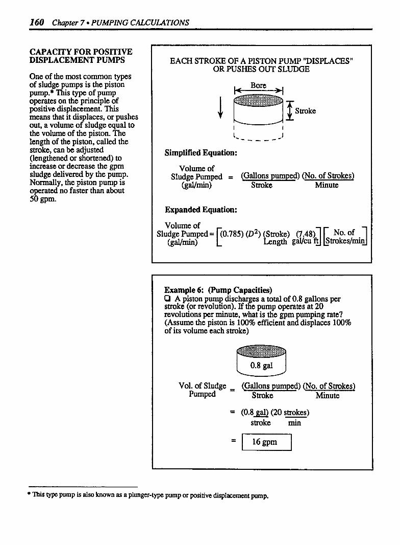
160 Chapter 7 PUMPING CALCULATIONS
CAPACITY FOR POSITIVE DISPLACEMENT PUMPS
One of the most common types of sludge pumps is the piston pump.* This type of pump operates on the principle of positive displacement. This means that it displaces, or pushes out, a volume of sludge equal to the volume of the piston. The length of the piston, called the stroke, can be adjusted (lengthened or shortened) to increase or decrease the gpm sludge delivered by the pump. Normally, the piston pump is operated no faster than about 50 gpm.
EACH STROKE OF A PISTON PUMP "DISPLACES" OR PUSHES OUT SLUDGE
Stroke
Simplified Equation:
Volume of Sludge Pumped = (Gallons pumped) (No. of Strokes)
( e b i n ) Stroke Minute
Expanded Equation:
Volume of Sludge Pumped = (02) (Stroke)
(gavmin) Length @/CU
Example 6: (Pump Capacities) P A piston pump discharges a total of 0.8 gallons per stroke (or revolution). If the pump operates at 20 revolutions per minute, what is the gpm pumping rate? (Assume the piston is 100% efficient and displaces 100% of its volume each stroke)
Vol. of Sludge - (Gallons pumped) (No. of Strokes) Pumped Stroke Minute
= (0.8pl) (20 strokes) stroke min
+ This type pump is also known as a plunger-type pump or positive displacement pump.

pump Capacities l61
Example 7: (Pump Capacities) O A slud e pump has a bore of 8 inches and a stroke length of 8 inches. If the pump operates at 50 strokes (or revolutions) per minute, how many gpm are pumped? (Assume the piston is 100% efficient and displaces 100% of its volume each stroke.)
l+ 0.67 ft 4 = 0.67 ft 8 in.
12 in./ft
vol. of sludge - - (Gallons pumped) (No. of Strokes) Pumped Stroke Minute
(D 2, (Stroke) Length gdcu
(0.67 ft) (0.67 ft) (0.25 ft) (7.48
- - (0.66 gal) (50 strokes) stroke min
Example 8: (Pump Capacities) C l A sludge ump has a bore of 6 inches and a stroke setting of 3 inches. h e pump operates at 45 revolutions per minute. If the pump operates a total of 80 minutes during a 24-hour period, what is the gpd pumping rate? (Assume the piston is 100% efficient.)
0.5 ft +l .; <E:$@;$@s@.$g@.: :+. 6 in. .:.~.~.~~.~,~Z9~~xr.:.::~Fs':~~w.. ............ ......... ...S,...,.. s.~.:.:...~.:.:~ ..+ ...... A........ .. - = 0.5 ft 1 3 h. 12 in./ft - = 0.25 ft
12 in&
F i t calculate the gpm pumping rate: Vol. Pumped = (Gallons pumped) (No. of Strokes)
mm Stroke Minute
(0.5 ft) (0.5 ft) (0.25 ft) (7.48 CU
= (0.37 gal) (45 strokes) stroke min
= 16.7 gprn Then convert gpm to gpd pumping rate, based on total minutes pumped during 24-hours:
(16.7 gpm) (80 rnin) = - day
CALCULATING GPD PUMPED
There are two methods to determine gpd pumping rate:
Calculate the gprn pumping rate, then multiply by the total minutes operation during the 24-hour period:
Pumping , (Pumping) (Total +) Rate, gpd Rate, gpm PUmPW
in 24 hrs
Calculate the gallons pumped each revolution, then multiply by the total revolutions during the 24-hour period:
Pumping = (Gallons) (T.otal Revol.) Rate, Revolution day

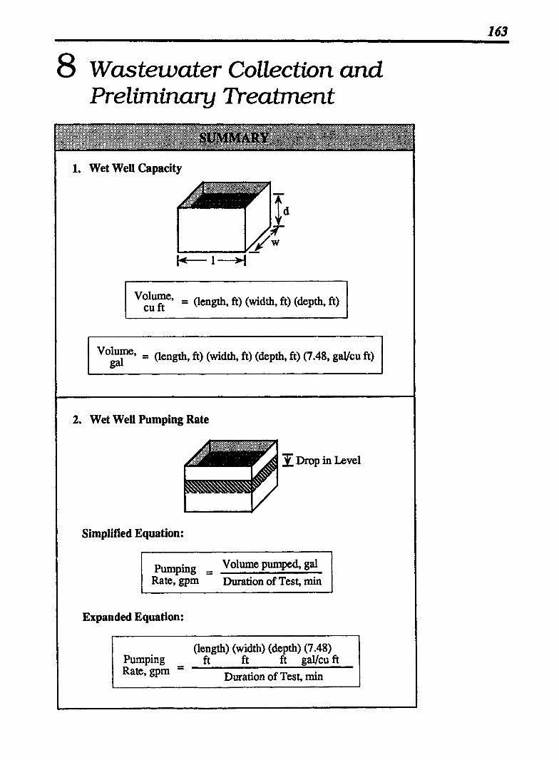
8 Wastewater Collection and Preliminary Treatment
1. Wet Well Capacity
vo1ume9 = (length, ft) (width, ft) (depth, ft) cu ft
= (length, ft) (width, ft) (depth, ft) (7.48, gucu ft) I 2. Wet Well Pumping Rate
Drop in Level
Simplified Equation:
pumping = Volume pumped, gal Rate, gpm Duration of Test, min
Expanded Equation:
(length) (width) (depth) (7.48) Pumping - ft ft ft gal/cu ft Rate, gpm - Duration of Test, min
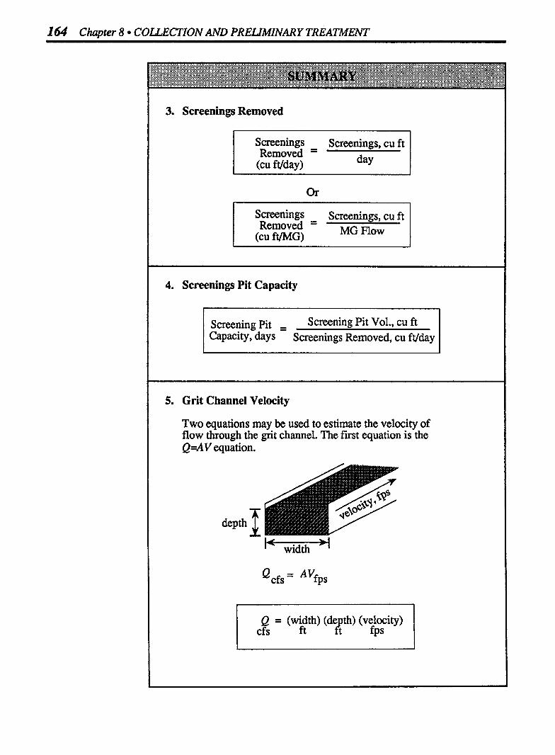
164 Chapter 8 COLLECTION AND PRELIMINARY TREATMENT
1 3. Screenings Removed
Screenings - Screenings, cu ft Removed -
(cu ft/MG) MG Flow
I 4. Screenings Pit Capacity
Screening Pit = Screening Pit Vol., cu ft Capacity, Screenings Removed, cu ft/day
5. Grit Channel Velocity
Two equations may be used to estimate the velocity of flow through the grit channel. The first equation is the Q=AV equation.
Q = (width) (de th) (velocity) cfs ft K fps

The second equation is necessary when using a float or dye to determine velocity.
Distance traveled, ft Velocity = Seconds of Test
Velocity = ,- ft l
I 6. Grit Removal
I Grit Removal Grit Volume, cu ft cu ft/MG Flow, MG
7. Flow measurement for a particular moment can be determined using the Q=AV equation. Metering devices often have instrumentation to read and record flow rates. However, charts, graphs and nomographs can also be used to estimate flow rates.
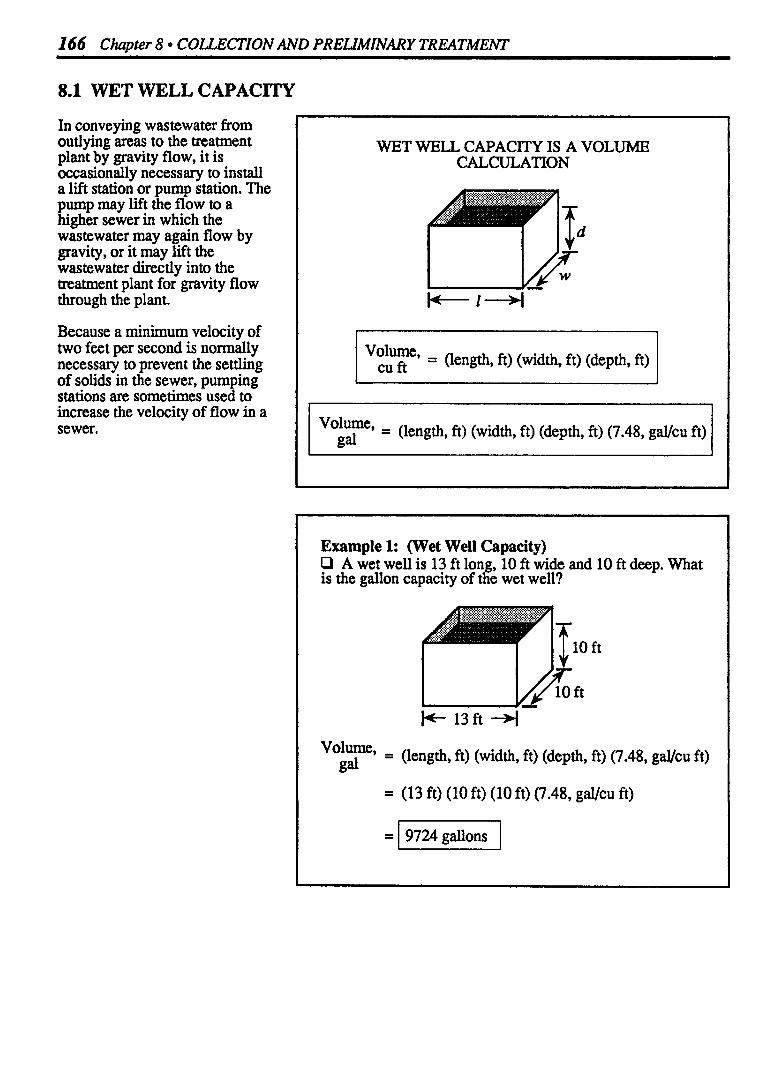
166 Chapter 8 COLLECTION AND PRELIMINARY TREATMENT
8.1 WET WELL CAPACITY
In conveying wastewater from outlying areas to the treatment plant by gravity flow, it is occasionally necessary to install a lift station or pump station. The pump may lift the flow to a higher sewer in which the wastewater may again flow by gravity, or it may lift the wastewater directly into the treatment plant for gravity flow through the plant.
Because a minimum velocity of two feet per second is normally necessary to prevent the settling of solids in the sewer, pumping stations are sometimes used to increase the velocity of flow in a sewer.
WET WELL CAPACITY IS A VOLUME CALCULATION
I vtuy' = (length, ft) (width, ft) (depth, ft) /
volume, = (length, ft) (width, ft) (depth, ft) (7.48, gal/cu ft) I gal
Example 1: (Wet Well Capacity) P A wet well is 13 ft long, 10 ft wide and 10 ft deep. What is the gallon capacity of the wet well?
I vo1ume9 = (length, ft) (width, ft) (depth, ft) (7.48, g a b ft) gal
= (13 ft) (10 ft) (10 ft) (7.48, gal/cu ft) l
= 1 9724 gallons I

Wet Well Capacity 167
Example 2: (Wet Well Capacity) D A wet well is 8 ft long, 6 ft wide and 6 ft deep. what is the gallon capacity of the wet well?
(length, ft) (width, ft) (depth, fi) (7.48, gaVcu ft)
(8 ft) (6 ft) (6 ft) (7.48, gaVcu ft)
1 2154 gallons I
Example 3: (Wet Well Capacity) O A wet well 12 ft long and 10 ft wide contains wastewater to a depth of 3.7 ft. How many gallons of wastewater are in the wet well?
volume, = (length, ft) (width, ft) (depth, ft) (7.48, gdcu ft) gal
= (12 ft) (10 ft) (3.7 ft) (7.48, gdcu ft)
= 1 3321 gallons I
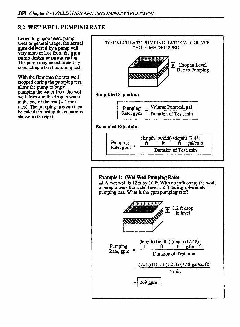
168 Chapter 8 COLLECTION AND PRELIMINARY TREATMENT
8.2 WET WELL PUMPING RATE
Depending upon head, pump wear or general usage, the actual gpm delivered by a pump will vary more or less from the gpm pump design or pump rating. The pump may be calibrated by conducting a brief pumping test.
With the flow into the wet well stopped during the pumping test, allow the pump to begin pumping the water from the wet well. Measure the drop in water at the end of the test (2-5 min- utes). The pumping rate can then be calculated using the equations shown to the right.
TO CALCULATE PUMPING RATE CALCULATE "VOLUME DROPPED"
Drop inLevel Due to Pumping
Simplified Equation:
pumping = volume Pumped, gal Rate, gpm Duration of Test, min
Expanded Equation:
(length) (width) (depth) (7.48) ft ft ft gal/cuft - I Rate;gpm -
Duration of Test, min
Example 1: (Wet Well Pumping Rate) Q A wet well is 12 ft by 10 ft. With no influent to the well, a pump lowers the water level 1.2 ft during a 4-minute pumping test. What is the gpm pumping rate?
1.2 ft drop in level
(length) (width) (depth) (7.48) Pumping ft ft ft aa4cu ft - - Rate, gprn - Duration of Test, min
(12 ft) (l0 ft) (1.2 ft) (7.48 gdcu ft) - 4 min
= 1 269 gprn I

Wet Well Pwnping Rate 169
Example 2: (Wet Well Pumping Rate) O A wet well is 8 ft by 10 ft. Durin a 2-minute pumping test (with no influent to the wet we& the water level dropped 5 inches. What is the gpm pumping rate?
5 in. drop in level due to pumping
5 in. = 0.42 ft
(length) (width) (depth) (7.48) Pumping - ft ft ft gaVcu ft Rate, gpm - Duration of Test, min
- (8 ft) (10 ft) (0.42 ft) (7.48 gal/cu ft) 2 min
Example 3: (Wet Well Pumping Rate) D The de th of wastewater in a wet well is sufficiently low K to allow S utting off all pumps. With a rod and a stopwatch, you are able to determine that the water level rises 1.5 ft in 2 minutes 30 seconds. The pumps are restarted. What is the gpm influent rate to the 8 ft long, 8 ft wide wet well?
8
1.5 ft rise in level
I I/
(length) (width) (Rise in Level) (7.48) -
Pumping - ft ft ft gdcu ft Rate, gpm - Duration of Test, min
- - (8 ft) (8 ft) (1.5 ft) (7.48 ga4cu ft) 2.5 rnin
GIVEN INCHES DROP IN LEVEL
When the drop in water level is measmd in inches, the inches must first be converted to feet before using the pumping rate equation. Example 2 illustrates such a calculation.
CALCULATING INFLUENT RATE
This same basic concept can be used to estimate the flow rate of the water entering the wet well. An example of this type of cal- culation is given in Example 3.

170 Chapter 8 COLLECTION A N ' PRELIMINARY TREATMENT
8.3 SCREENINGS REMOVED
Scnens are used in pretreatment to remove large debris such as rags, cans, cardboard, etc., h m the wastewater flow. A range of 0.5 to 12 cu ft screenings per million gallons of flow may be removed from a plant. The withdrawal rate may remain somewhat stable for a plant, &pending on sources of wastewater flow.
In order to plan properly for screenings disposal, it is important to keep a record of the amount of screenings removed from the wastewater flow. Two methods commonly used to calculate the volume of scntnings withdrawn are:
Scretnings Screenings, cu ft Removed = (CU Way) days
Smnings Screenings, cu ft Removed = (cu ft/MG) Flow, MG
Examples 1 and 2 illustrate the fmt calculation, and Examples 3 and 4 illustrate the second calculation.
Example 1: (Screenings Removed) P A total of U allons of screenings m removed from the wastewater ff ow during a 24-hour period What is the screenings removal reported as cu ft/day?
First, convert gallons screenings to cu ft:*
Now calculate screenings removed as cu ftlday:
7.4 c, ft Removed = (CU fmy) 1 &Y
Example 2: (Screenings Removed) 0 During one week, a total of 290 gallons of screenings were =moved h m the wastewater screens. What is the average screenings removal in cu ft/day?
First, gallons screenings must be converted to cu ft scncnings:
Now the screenings removal calculation can be completd
38.8 cu ft Removed = (cu ftfday) 7 days
* For a review of gal to cu ft conversions, refer to Chapter 8 in Bosic Math Concepts.

Screenings Removed 171
Example 3: (Screenings Removed) P The flow at a treatment plant is 3.6 MGD. If a total of 5.5 cu ft screenings are removed during the 24-hour period, what is the screenings removal reported as cu ft/MG?
Saeenings Screenings, cu ft Removed = (cu WMG) Flow, MG
- - 5.5 cu ft 3.6 MG
Example 4: (Screenings Removed) P On a articular day a treatment plant receives a flow of 3,850,008 gpd. If 80 gallons of screenings are removed that day, what is the screenings removal expressed as cu ft/MG?
First, convert gallons screening to cu ft:
Now calculate the desired screening rate. Remember that the flow must be expressed in million gallons:
Saeenings Screenings, cu ft Removed = (cu ft/MG) Flow, MG

172 Chapter 8 COLLECTION A N . PRELIMINARY TREATMENT
8.4 SCREENINGS PIT CAPACITY
Screenings pit capacity calcula- tions are actually detention time calculations.* Remember that detention time may be consid- ered the time required to flow through a tank or the time required to fill a tank or basin at a given flow rate. In screenings pit capacity problems, the time required to fill a screenings pit is being calculated.
Both the general fill time equa- tion and the specific equation to be used in screenings pit capacity problems are given below.
ill = volume of Tank, gal Time Flow Rate, gal/time
Screenings = Volume of Pit, CU ft Pit Fill Time, Screenings Removed,
Example 1: (Screenings Pit Capacity) P A screenings pit has a ca acity of 400 cu ft. (The pit is actually larger than 400 cu if to accommodate soil for covering.) If an average of 3.4 cu ft of screenings are removed daily from the wastewater flow, in how many days will the pit be full?
400 cu ft Volume
Fill Time, - - Volume of Pit, cu ft days Screenings Removed, cu ft/day
Example 2: (Screenings Pit Capacity) Q A lant has been averaging a screenings removal of P 2 cu t/MG. If the average dady flow is 1.6 MGD how many days will it take to fill the pit with an available capacity of 150 cu ft?
150 cu ft Volume
The filling rate must first be expressed as cu ft/day:
(2 cu ft) (1.6 MGD) = 3.2 cu ft/day - MG
Now calculate fill time:
Fill Time, - - 150 cu ft days 3.2 cu ft/day
* For a review of detention time calculations, refer to Chapter 5.

Example 3: (Screenings Pit Capacity) P A skenings it has a capacity of 1-0 cu yds available for screenings. Qthe plant removes an average of 2.4 cu ft of screenings per day, in how many days will the pit be filled?
10 cu yds Volume
Since the filling rate is expressed as cu Wday, the pit volume must be expressed as cu ft:**
(10 cu yds) (27 cu ft) = 270 cu ft cu yds
Now calculate fill time:
Fill Time, - - Volume of Pit, cu ft days Screenings Removed, cu ftlday
= 1 112.5 days I
Example 4: (Screenings Pit Capacity) Q Suppose you want to have a screenings pit capacity of 90 days (not including dirt for cover). If the scnenings removal rate is 4 cu ft/&y, what will the available volume of the screenings pit have to be (cu ft)?
Fill Time, , - Volume of Pit, cu ft days Screenings Removed, cu f t b y
CALCULATING OTHER UNKNOWN VALUES
In Examples 1 3 the unknown variable was fill time. However, other variables such as the required pit volume or the filling rate can also be the unknown variable. Example 4 illustrates this type of calculation.
* * To review cu yd to cu ft conversions, refer to Chapter 8 in Baric Math Concepts.

174 Chapter 8 COLLECTION AND PRELIMINARY TREATMENT
8.5 GRIT CHANNEL VELOCITY
Thc desired velocity in sewers is approximately 2 fps at peak flow, because this velocity will normally prevent solids from settling from the lines. However, when the flow naches the grit channel, the velocity is decreased to about l fps to permit settling of the heavy inorganic solids. These solids are =moved early in the treatment process because they produce an unnecessary load on biological processes and greater stress on mechanical equipment.
There are two methods used to estimate the velocity of flow in a grit channel-the Q=AV method and the float or dye method.
VELOCITY USING Q=AV
The Q=AV equation may be used to estimate the velocity of flow in a channel or pipeline. Write the equation, filling in the known data, then solve for the unknown factor (velocity in this case).
Be sure that the volume and time expressions match on both sides of the equation. For instance, if the velocity is desired in ftlsec, then the flow rate should be converted to cu ftfsec befon beginning the Q=AV calculation. Examples 1 and 2 illustrate a velocity estimate using the Q=AV equation.
Example l: (Grit Channel Velocity) Q A grit channel is 2.5 ft wide, with water flowing to a depth of 14 inches. If the flow meter indicates a flow rate of 1450 gpm, what is the velocity of flow through the channel?(fps)
Convert ern to cfs:
1450 gpm (7.48 gal) (60 sec)
7
tuft min = 3.2 cfs
3.2 cfs = (2.5 ft) (1.17 ft) (X @S)
1 1.1 fps 1 = X
Example 2: (Grit Channel Velocity) C) The total flow through both channels of a grit channel is 5.9 cfs. If each channel is 2 ft wide and water is flowing to a depth of 15 inches, what is the velocity of flow through the channels? (fps)
Qcfs = AV@,
5.9 cfs = (4 ft) (1.25 ft) (X @S)

Grit Channel Velocity 175
Example 3: (Grit Channel Velocity) P A stick travels 35 ft in 30 seconds in a grit channel. What is the estimated velocity in the channel (ft/sec)?
30 sec
Velocity - Distance, ft - ftfsec Time, sec
- 35 ft -- 30 sec
Example 4: (Grit Channel Velocity) O A stick is placed in a grit channel and flows 19 ft in 15 seconds. What is the estimated velocity in the channel
p a t
15 sec
Velocity - Distance, ft ft/sec Time, sec
19 ft -- 15 sec
VELOCITY USING THE FLOAT OR DYE METHOD
Velocities can also be estimated by the use of a float placed in the water. By timing the distance traveled by the float, the velocity can be determined:
velocity Distance, ft Time, sec I
Remember that these velocity calculations are estimates only. Since a float or stick tends to move along with the faster surface waters, the calculated velocity can be as much as 10 or 15 percent faster than the actual average flow rate.
Other flow patterns and currents through the channel can also affect the flow velocity of the float or stick, even slowing it somewhat.
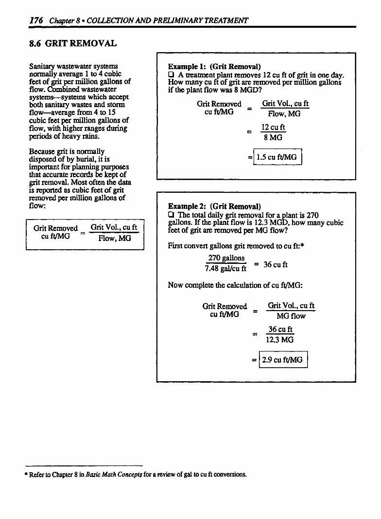
I76 Chapter 8 COLLECTION AND PRELIMINARY TREATMENT
8.6 GRIT REMOVAL
Sanitary wastewater systems nomally average 1 to 4 cubic feet of grit per million gallons of flow. Combined wastewater systems-systems which accept both sanitary wastes and storm flow-average from 4 to 15 cubic feet per million gallons of flow, with higher ranges during periods of heavy rains.
Because grit is normally disposed of by burial, it is important for planning purposes that accurate nxords be kept of grit removal. Most often the data is reported as cubic feet of grit removed per million gallons of flow:
Example 1: (Grit Removal) O A treatment plant removes 12 cu fi of grit in one day. How many cu ft of grit are removed per million gallons if the plant flow was 8 MGD?
Grit Removed - Grit Vol., cu ft cu ft/MG - Flow, MG
Example 2: (Grit Removal) C l The total daily grit removal for a lant is 270 g gallons. If the plant flow is 12.3 MG , how many cubic feet of grit are removed per MG flow?
First convert gallons grit removed to cu ft:*
270 gallons 7.48 gal/cu ft = 36cuft
Now complete the calculation of cu ft/MG:
Grit Removed - Grit Vol., cu ft cuft/MG MG flow
* Refer to Chapter 8 in Basic Math Comepts for a review of gal to cu ft conversions.

Grit Removal 177
Example 3: (Grit Removal) P The avera e 't removal at a particular treatment lant is 2.1 cu d ~ . % ? t h e monthly average daily flow is 8.5 MGD, how many cu yds of grit would be removed from the wastewater flow during one month? (Assume the month has 30 days.)
First calculate the cu ft grit removed from the average daily flow:
(2.1 cu ft) (4.5 MGD) MG = 9.45 cu ft
each day Then calculate the anticipated grit removed for the month:
(9.45 cu ft) (30 days) day
= 283.5 cu ft
And convert cu ft grit removed to cu yds grit:
283.5 cu ft 27 cu ft/cu yds
l
FORECASTING DISPOSAL NEEDS
Over a given time, the average grit removal rate at a plant (at least a seasonal average) can be determined and used for planning purposes. Oftem grit removal is calculated as cubic yards, since excavation is noxmally expnssed in terms of cubic yards. *
Total Grit, cu ft = cu yds grit
27 cu ft/cu yds
Example 4: (Grit Removal) P The monthly average 't removal is 3 cu W G . If the monthly average flow is &0,000 gpd, how many cu yds must be available for grit disposal if the disposal pit is to have a 90-day capacity?
First calculate the grit generated each day:
(3 cu ft) (2.8 MGD) - - - 8.4 cu ft MG each day
The cu ft grit generated for 90 days would be:
(8.4 cu ft) (90 days) day
= 756cuft
Converting cu ft grit to cu yds grit:
756 cu ft 27 cu ft/cu yds
* Cu ft to cu yds conversions are described in Chapter 8 of Basic Math Concepts.

178 Chapter 8 COLLECTION AND PRELlMINARY TREATMENT
8.7 FLOW MEASUREMENT
FLOW MEASUREMENT USING Q=AV
The flow rate through grit channels is normally measured by some type of flow metering &vice as described in the following pages. However, the flow rate for any particular moment can also be determined by using the Q=AV equation.
The flow rate (Q) is equal to the cross-sectional area (A) of the channel or pipeline multiplied by the velocity (V) through the channel.
FLOW MEASUREMENT USING Q=AV
BE SURE THAT VOLUME AND TlME TERMS MATCH ON
BOTH SIDES OF THE EQUATION
Example 1: (Flow Measurement) D A grit channel 2 ft wide has water flowin to a depth of 1.5 ft. If the velocity through the channel is f.2 fps, what is I the cfs flow rate thiough the channel?
Qcfs = Ahps
= (2 ft) (1.5 ft) (1.2 @S)
=l 3.6 cfs

Flow Measurement 179
Example 2: (Flow Measurement) Q A grit channel 30 inches wide has water flowing to a depth of 1 ft. If the velocity of the water is 1.3 @S, what is the cfs flow in the channel?
Qcfs = AVf*s
= (2.5 ft) (1 ft) (1.3 @S)
=l 3.25 cfs I
Example 3: (Flow Measurement) O A grit channel 2 ft wide has water flowing at a velocity of 0.9 fps. If the depth of water is 1.25 ft, what is the gpd flow rate through the channel? (Assume the flow is steady and continuou~)
1.25 f$
Qcfs = AVfps
= (2 ft) (1.25 ft) (0.9 fps)
= 2.25 cfs
Now convert cfs flow rate to gpd:
(2.25 cu ft) (60 sec) (7.48 gal) (1440 min) = 1,454,112 gpd - - - sec rnin cu ft day
DIMENSIONS SHOULD BE EXPRESSED AS FEET
The dimensions in a Q=AV calculation should always be expressed in feet because (ft) (ft) (ft) = cu ft. Therefore when dimensions are given as inches, first convert all dimensions to feet before beginning the &=AV calculation.
CALCULATING GPM OR GPD FLOW
If gpm or gpd flow rate is desired, simply calculate the cfs flow rate, as illustrated in Examples 1 and 2, then convert cfs flow to gpm or gpd flow rate.*
* To review flow conversions, refer to Chapter 8 in Basic Math Concepts.
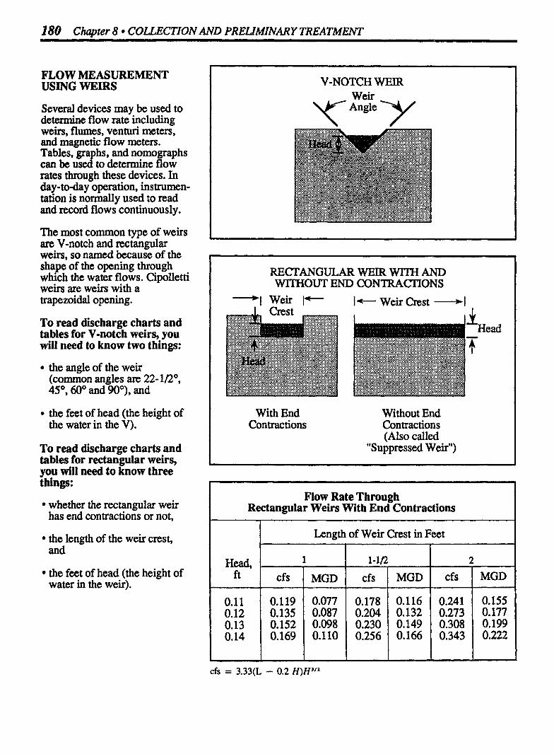
180 Chapter 8 COLLECTION AND PRELIMINARY TREATMENT
FLOW MEASUREMENT USING WEIRS
Several devices may be used to determine flow rate including weirs, flumes, venturi meters, and magnetic flow meters. Tables, graphs, and nornographs can be used to determine flow rates through these devices. In day-to-day operation, instrumen- tation is normally used to read and record flows continuously.
The most common type of weirs are V-notch and rectangular weirs, so named because of the shape of the opening through which the water flows. Cipolletti weirs are weirs with a trapezoidal opening.
To read discharge charts and tables for V-notch weirs, you will need to know two things:
the angle of the weir (common angles an 22- lnO, 4S0, 60° and WO), and
the feet of head (the height of the water in the V).
To read discharge charts and tables for rectangular weirs, you will need to know three things:
whether the rectangular weir has end contractions or not,
the length of the weir crest, and
the feet of head (the height of water in the weir).
V-NOTCH WEIR
RECTANGULAR WEIR WITH AND WITHOUT END CONTRACTIONS
-1 Weir b- Weir Crest -1
With End W~thout End Contractions Contractions
(Also called "Suppressed Weir")
Flow Rate Through Rectangular Weirs With End Contractions
Length of Weir Crest in Feet I 1

Flow Measurement I81
FLOW THROUGH A 90' V-NOTCH WEIR+=~.SH~/~
n w OM WEIR- FELT
Source: New York Manual of Instruction for Water Tmatment Plant Operators
Example 4: (Flow Measurement) P Use the flow table to detenaine the MGD flow rate through a rectangular weir with end contractions if the feet of head indicated at the staff gage is 0.14 ft and the length of the weir crest is 1 .S ft.
First find 0.14 ft in the "Head column. Then move to the right until you come under the column 1 112. The MGD reading is 0.166 MGD
Example 5: (Flow Measurement) O The head on a V-notch weir is 0.5 ft. What is the cfs flow through the weir? (Use the graph above to determine flow rate.)*
The bottom of the chart indicates flow rate in feet. Find 0.5 ft and follow the line upward to the diagonal line. Then move horizontally to the left scale. The line falls halfway between the 0.4 and 0.5. So the reading is about 0.45 cfs.
/ 0.45 cfs I C For a discussion of reading scales. refer to Chapter 12 in Basic Math Concepts.

182 Cha~ter 8 COLLECTION AND PRELlMINARY TREATMENT
FLOW MEASUREMENT USING PARSHALL FLUMES
One of the most commonly used flow measuring devices is the Parshall flume. A Parshall flume is a specially designed constriction in an open channel. The water flows into the converging section, then drops down through the throat section and out into the diverging section. Parshall flumes are classified according to throat width, W.
Parshall flumes are often favored over weirs for flow measurement since the flumes are self-cleaning (there are no places for debris to get lodged) 6 d there is very little head loss in this type of flow measurement device.
Flow measurement for a Parshall flume is based on the depth of water (head) measured at H, in the converging section. To use the flow charts or graphs, you must know whether there are free flow conditions or submerged flow conditions in the flume.
PARSHALL FLUME
I Section I Converging Diverging Section Section
Top View
Submerged Flow ll Conditions
for Ha and H b Free Flow Conditions
Side View
I DISCHARGE OF 6-INCH PARSHALL FLUME
Head ( cfs ft
cfs = 2.06H1-s8
gps I MGD Head 1 cfs I gps ft MGD

Example 6: (Flow Measurement) O The head measured at the upstream ga e on a 6-inch Parshall flume is 0.38 ft. What is the MG 8 flow through the channel? (Assume there are no submergence conditions in the channel.)
First, find 0.38 ft in the head column. Then move to the right to the MGD flow rate column:
Example 7: (Flow Measurement) 01 What is the cfs flow through a 6-inch Parshall flume if the upstream gage indicates a depth of 0.35 ft? (Assume no submergence condition exists.)
Find 0.35 ft in the head column. Then move to the right to the cfs column. The flow rate indicated is:
1 0.3922 cfs I
Example 8: (Flow Measurement) O The head measured at the upstream gage of a 6-inch Parshall flume is 0.45 ft. What is the gpm flow through the flume? (Assume no submergence condition exists.)
First determine the gps flow rate indicated:
4.364 gps
Then convert gps flow to @m:*
sec
PARSHALL FLUME-FREE FLOW CONDITIONS
Free flow conditions means there are no downstream conditions causing the water to "back up" or restrict the water flowing out of the flume.
For frec flow conditions, only the upstream depth measuremnt (& ) is needed to determine flow through the flume. Examples 6-8 illustrate calculations when free flow conditions exis to
The table shown on the previous page is a partial table of heads and corresponding flow rates for a 6-inch Parshall flume. Refer- ence handbooks contain tables for various throat widths and head conditions.
* For a review of flow conversions refer to Chapter 8 in Basic Math Concepts.

184 Chapter 8 COLLECTION AND PRWMINARY TREATMENT
PARSHALL FLUME 4UBMERGED CONDITIONS
Submerged flow conditions indicate that there are down- stream conditions which restrict the free flow of water and result in a false or inaccurate depth reading. Because the water is "backed up", the depth reading at Ha is higher than actual flow conditions would warrant.
To determine whether sub- merged flow conditions exist, calculate the percent submer- gence. Remember, percent equals "part over whole". Them fon since the downstream depth indicates the part submergence, percent submergence is calcu- lated as:
% Submerg. = Part Submerg. Total
This equation can be restated as:
% Submergence = - X 100 Ha Hb I
Submerged conditions exist when the percent submergence exceeds:
50% for flumes 1 in., 2 in. and 3 in. wide,
60% for flumes 6 in. and 9 in. wide,
70% for flumes 1 to 8 ft wide, and
80% for flumes 8 to 50 ft wide.
PARSHALL FLUME NOMOGRAPH
- a W 60 70 80 q(r l00
Submergence. HbIHs, in Percentage
Reprinted with permission of Public Works Magazine, Szptcmber, October, and November 1968 issues.

Example 9: (Flow Measurement) O What is the cfs flow through a Parshall flume with a throat width of 3 ft if the water depth at the upstream gage is 14 inches? The downstream depth (Hb) is 11 inches.
First determine the flow rate indicated by the nomograph. Place a straight-edge at the mark on the width scale to the left. Then while holding the top of the straight-edge on the 3 mark, rotate the straight-edge until it lines up with the 14 mark on the left side of the middle scale. Now draw a line from the 3 mark, through the 14 and on to the scale on the right side.
The flow rate scale is marked off for gpm on the left side and cfs on the right side. The cfs flow rate indicated is 15 cfs.
Now that the flow rate has been determined, we must detemine whether a correction factor is required. There- fore percent submergence must be determined:
Hb % Submergence = - X 100 H a
For a 3 ft Parshall flume, submergence exists when the percent exceeds 70%. Therefore the correction factor graph must be used to determine the appropriate correction factor.
First, find 79% on the bottom scale and move upward to the 3 ft throat width curve. Then move directly left to the scale. The comction factor indicated is 0.95. Multiply the flow rate determined from the nomograph (1 5 cfs) by the correction factor:
(15 cfs) (0.95) = 14.25 cfs El
Where submerged conditions exist, a correction factor must be used with values shown in the table or on a nomograph. Using the percent submergence, you use a graph to determine the correction factor needed. Then multiply the flow rate obtained in the table or on the nomo- graph by the correction factor. Example 9 illustrates the use of a nomograph in determining Parshall flume flow rate. The correction factor graph is also used in this example.
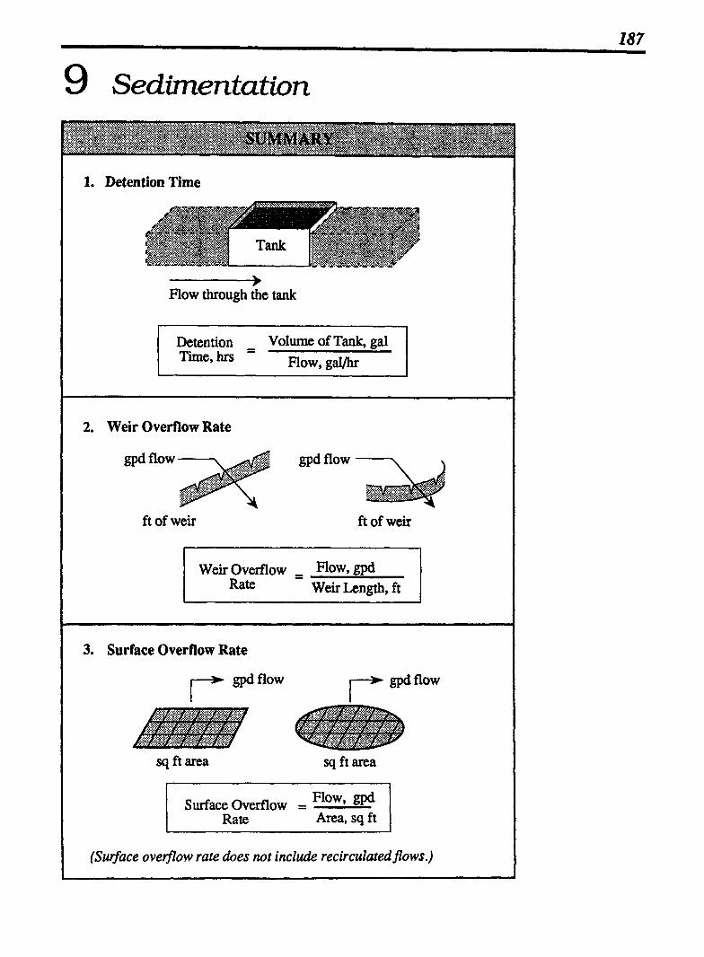
9 Sedimentation
1. Detention Time
Flow through the tank
Detention - Volume of Tank, gal Time, hrs
- mow, g m
2. Weir Overflow Rate
ft of weir ft of weir
Weir Overflow - - How, gpd Rate Weir Length, f't
3. Surface Overflow Rate
T' ppd flow
sq ft area sq ft area
Surface Overflow = Flow, gpd
Rate Area, sq ft
(Surface overfow rate does not include recirculated flows.)

188 Chapter 9 SEDIMENTATION
4. Solids Loading Rate (Secondary Clarifier) T
I I
P.E. Flow
r' I 8
P.E. Aeration I Tank I/*'
Simplified Equation:
"lids Solids Applied, lbs/day Loading = Rate Surface Area, sq ft
Expanded Equation:
I Rate (0.785) (02) I
5. BOD and Suspended Solids Removed, lbdday
BOD or SS Removed ( m m
First calculate BOD or SS removed. m&
Influent - Effluent = Removed BODorSS BODorSS BODorSS
mg/L mg/L mg/L
Then calculate lbs/day BOD or SS removed;
(mg/L) (MGD) (8.34) = lbs/day BODorSS flow lbs/gal BODorSS Removed Removed
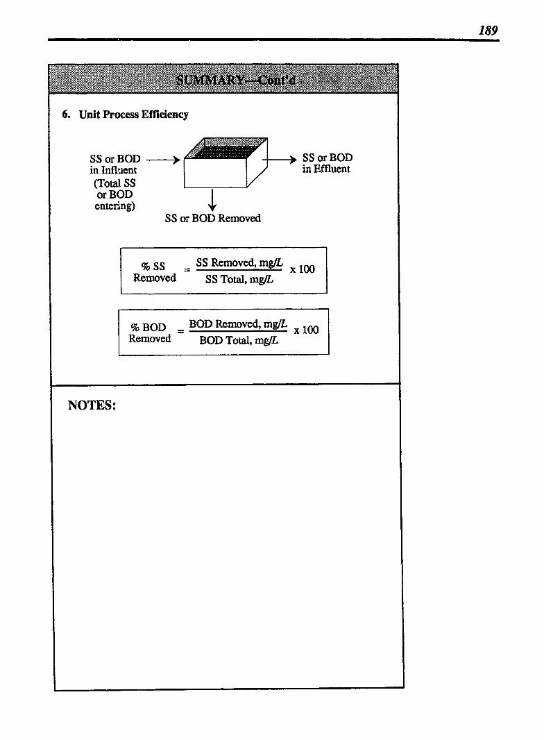
SS or BOD SS or BOD -
I I / in Influent in Effluent (Total SS or BOD
U entering) 4
SS or BOD Removed
% S S = SS Removed, mg/L Removed SS Total, mgll.
% BOD = BOD Removed, mglL 100 hnoved BOD Total, mglL

190 Chapter 9 SEDIMENTATION
9.1 DETENTION TIME
The detention time for clarifiers may vary from one to three hours. The equation used to calculate detention time is:
Detention = Volume of Tank, gal Time, hrs Flow Rate, gph
MATCHING UNITS
There are many possible ways of calculating detention time, depending on the time unit desired (seconds, minutes, hours, days) and the expression of volume and flow rate.
When calculating detention time, therefore, it is essential that the time and volume units used in the equation are consistent on both sides of the equation, as illustrated to the right.
The flow rate to the clarifier is normally expressed as MGD or gpd. However, since the detention time is desired in hours, it is important to express the flow rate in the same time frame-gal/hr (or @h):*
I - -
Flow, .= Flow, gph 24 hrsfday
DETENTION TIME IS FLOW-THROUGH TIME
D.T. - - Volume of Tank, gal hrs Flow Rate, gph
BE SURE YOUR TIME AND VOLUME UNITS MATCH
Detention Time = Volume of Tank, gal hrs A
I -.l
Time units match (W Volume units
match (gal)
Example 1: (Detention Time) P The flow to a sedimentation tank 70 ft long, 25 ft wide, and 10 ft dwp is 2.78 MGD. What is the detention time in the tank, in hours?
25 ft Tank Volume:
(70 ft) (25 ft) (10 ft) (7.48 gaVcu ft) 10 ft = 130,900 gal
First, MGD flow rate must be converted to gph so time units will match. (2,780,000 gpd + 24 hrdday = 115,833 gph.) Now fill in the equation and solve for the unknown.
Detention Time - - Volume of Tank, gal hrs Flow Rate, gph
- - 130,900 gal 115,833 gph
+ For a review of flow rate conversions, refer to Chapter 8 in Bosic Math Concepts.

Detention Time 191
Example 2: (Detention Time) O A circular clarifier receives a flow of 4,752,000 gpd. If the clarifier is 65 ft in diameter and 12 ft deep, what is the clarifier detention time? (Assume the flow is steady and continuous.)
l L L J = 297,700 gal
First, convert the flow rate from gpd to gph so that time units will match. (4,752,000 gpd t 24 hrs/day = 198,000 gph). Then calculate detention time:
- - 297,700 gal 198,000 gph
Example 3: (Detention Time) D A circular clarifier has a ca acit of 120,000 gallons. If the flow to the clarifier is 1,6&,dgpd, what is the clarifier detention time? (Assume the flow is steady and continuous.)
Volume B First, convert the flow rate from gpd to gph so that time units will match. (1,600,000 gpd + 24 hrs/day = 66,667 gph). Then calculate detention time:
Detention Time - Volume of Tank, gal hrs Flow Rate, gph
- - 120,000 gal 66,667 gph

192 Chapter 9 SEDIMENTATION
9.2 WEIR OVERFLOW RATE
The calculation of weir overflow rate is important in detecting high velocities near the weir which affixt the efficiency of the sedimentation process. With excessively high velocities near the weir, the settling solids are pulled over the weirs and into the effluent troughs, thus preventing desind settling.
Weir overflow rate is a measure of the gallons per day flowing over each foot of weir. (The weir overflow rate may be less for secondary clarifiers-5,000- 15,ooo gpd/ft).
WEIR OVERFLOW RATE
gpd flow . ..&, ;@p p j flow --&
..:?$#&.p. ..:&.&:;.:W. .,: yYYYYY.a 25.. . S:. y
-.v.. . . . ,: Y . *a.; .:>?:$.. .* ;;4$$5::F
$*P q@....$.+&$..:w +
ft of weir ft of weir
WEIR OVERFLOW WEIR OVERFLOW Rectangular Clarifier Circular Cldier
Weir Overflow - Flow, gpd I Rate -
Weir Length, ft
Example 1: (Weir Overflow Rate) P A rectangular clarifier has a total of 90 ft of weir. What is the weir overflow rate in gpd/ft when the flow is
....tf.
.......... ..:*.@:i.$w'- ..X..<~X~ .~.'.' .....S. x.:.;h .... &..... .,.& . . . . . .
$py>$~F :;::p'
90 ft weir
Weir Overflow , Flow, gpd Rate Weir Length, ft
- - 1,098,000 gpd 90 ft

Weir Gverfow Rate 193
Example 2: (Weir Overflow Rate) O A circular clarifier nxeives a flow of 3.6 MGD. If the diameter of the weir is 80 ft, what is the weir overflow rate in gpd/ft?
The total fi of weir is not given directly in this problem. However, weir diameter is given (80 ft) and from that information, the total ft of weir can be determined.
ft of weir: = (3.14) (80 ft) = 251 ft
Weir Overflow = Flow, gpd Rate Weir Length, ft
Example 3: (Weir Overflow Rate) CI A clarifier receives a flow of 1.87 MGD. If the diameter of the weir is 60 ft, what is the weir over flow rate in gpd/ft?
First calculate the gpd flow, then express the answer in I MGD.
Weiroverflow - - Flow, gpd Rate Weir Length, ft
- - 1,870,000 gpd (3.14) (60 ft)
CALCULATING WEIR CIRCUMFERENCE
In some calculations of weir overflow rate, you will have to calculate the total weir length, given the weir diameter. To calculate the length of weir around a circular clarifier, you need to know the relationship between the diameter and circumference of a circle. The distance around any circle (circumference) is about three times the distance across that circle (diameter). Or more precisely, the circurnfemce is 3.14 times the diameter. * Therefore, when you know the weir diameter, you can calculate the total feet of weir:
To'B.' Ft = (3.14) (Weir Diam.) of Welr in ft
* For a review of circumference calculations, refer to Chapter 9, "Linear Measurement", in Basic Math Concepts.
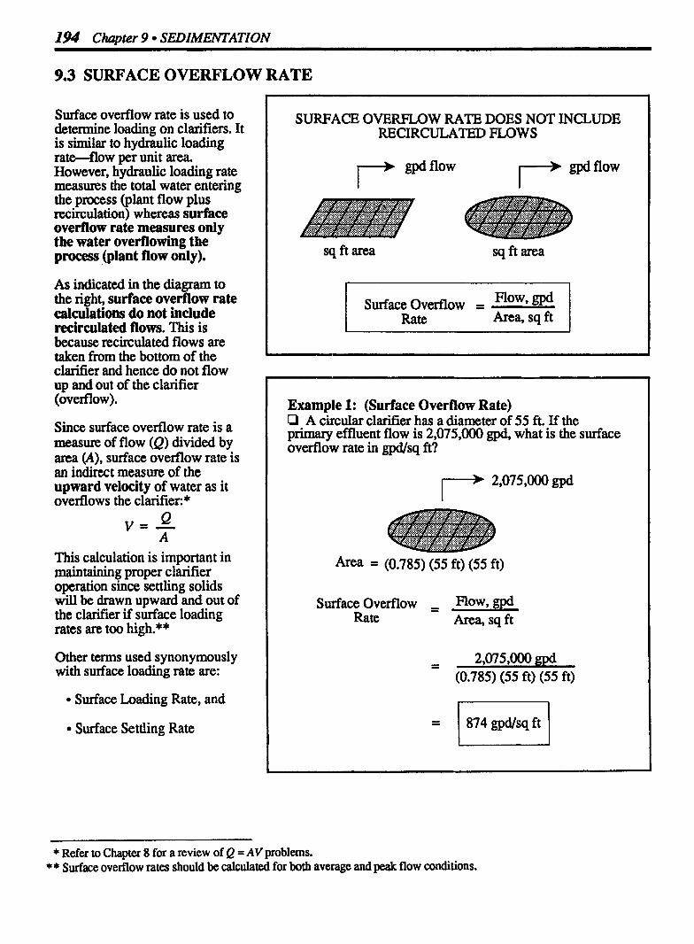
194 Chapter 9 SEDIMENTATION
9.3 SURFACE OVERFLOW RATE
Surface overflow rate is used to determine loading on clarifiers. It is similar to hydraulic loading rate-flow per unit area. However, hydraulic loading rate measures the total water entering the process (plant flow plus recirculation) whereas surface overflow rate measures only the water overflowing the process (plant flow only).
As indicated in the diagram to the right, surface overflow rate calculations do not include recirculated flows. This is because recirculated flows are taken from the bottom of the clarifier and hence do not flow up and out of the clarifier (overflow).
Since surface overflow rate is a measure of flow (Q) divided by area (A), surface overflow rate is an indirect measure of the upward velocity of water as it overflow S the clarifier: *
Q v = - A
This calculation is important in maintaining proper clarifier operation since settling solids will be drawn upward and out of the clarifier if surface loading rates are too high.**
Other terms used synonymously with surface loading rate are:
Surface Loading Rate, and
Surface Settling Rate
SURFACE OVERFLOW RATE DOES NOT INCLUDE RECIRCULATED FLOWS
sq ft area sq ft area
Surface Overflow = Rate Area, sq ft 1
Example 1: (Surface Overflow Rate) O A circular clarifier has a diameter of 55 ft. If the primary effluent flow is 2,075,000 gpd, what is the surface overflow rate in gpd/sq ft?
Area = (0.785) (55 ft) (55 ft)
SurfaceOverflow - ~ow,gpd Rate Area, sq ft
- - 2,075,000 gpd (0.785) (55 ft) (55 ft)
* Refer to Chapter 8 for a review of Q = AV problems. * * Surface ovefflow rates should be calculated for both average and peak flow conditions.
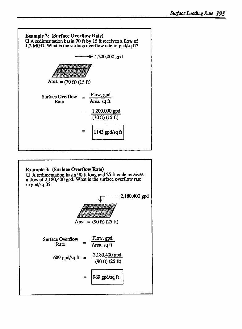
Swfoce b a d i n g Rate 195
Example 2: (Surface Overflow Rate) O A sedimentation basin 70 ft by 15 ft receives a flow of 1.2 MGD. What is the surface overflow rate in gpd/sq ft?
Area = (70 ft) (15 ft)
Surface Overflow = Flow, gpd Rate h sq ft
- 1,200,000 gpd - (70 ft) (15 ft)
Example 3: (Surface Overflow Rate) P A sedimentation basin 90 ft long and 25 ft wide receives a flow of 2J80.400 gpd What is the surface ovedlow rate in gpdjsq ft?
Area = (90 ft) (25 ft)
Surface Overflow - mow, gpd Rate - Area, sq ft
689 gpd/sq ft = 2,l 809400 gpd (90 ft) (25 ft)
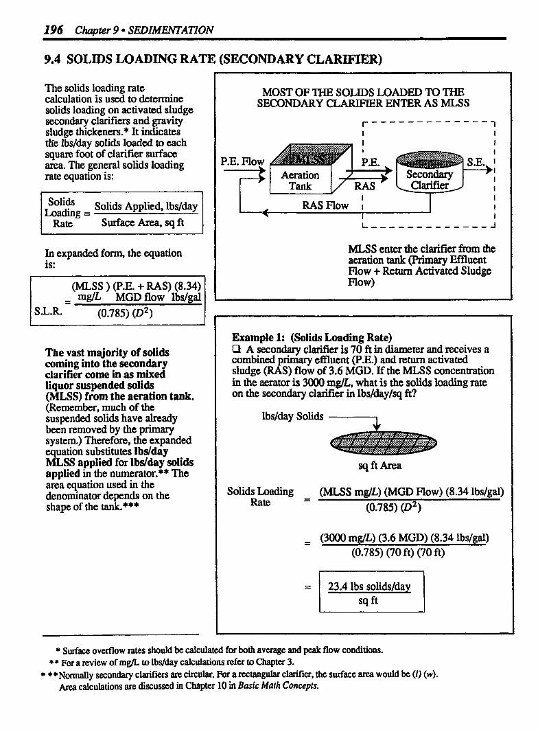
196 Chapter P SEDIMENTATION
9.4 SOLIDS LOADING RATE (SECONDARY CLARIFIER)
The solids loading rate calculation is used to determine solids loading on activated sludge secondary clarifiers and gravity sludge thickeners.* It indicates the ibs/&y solids loaded to each square foot of clarifier surface area. The general solids loading rate equation is:
Solids Applied, lbs/&y Loading = Rate Surface Area, sq ft
In expanded form, the equation is:
(MLSS ) (P.E. + RAS) (8.34) 1 - ' mglL 'MGD flow lbslgai
S.L.R. (0.785) (02)
The vast majority of solids coming into the secondary clarifier come in as mixed liquor suspended solids (MLSS) from the aeration tank. (Remember, much of the suspended solids have already been removed by the primary system.) Therefore, the expanded equation substitutes lbdday MLSS applied for Ibdday solids applied in the numerator. ** The area equation used in the denominator depends on the shape of the tank.***
MOST OF THE SOLIDS LOADED TO THE SECONDARY CLARIFIER ENTER AS MLSS
MLSS enter the clarifier f h m the aeration tank (Primary Effluent Flow + Return Activated Sludge Flow)
I RAS Flow I
Example 1: (Solids Loading Rate) P A secondary clarifier is 70 ft in diameter and receives a combined primary effluent (PE.) and return ac tivattd sludge (RAS) flow of 3.6 MGD. If the MLSS concentration in the aerator is 3000 m&, what is the solids loading rate on the secondary clarifier in lbs/day/sq fi?
I I
lbslday Solids 7
I I
sq ft Area
Solids Loading (MLSS mg/L) (MGD Flow) (8.34 lbslgal) Rate - -
(0.785) (D?)
( 3 0 mglL) (3.6 MGD) (8.34 lbslgal) (0.785) (70 ft) (70 ft)
23.4 lbs solidslday sq ft
+ Surface overtlow rates should be calculated for both average and peak flow conditions. * * For a review of mg/L to lbs/day calculations refer to Chapter 3.
* * *Normally sezondary clarifiers are circular. For a rectangular clarifier, the surface area would be (l) (W).
Area calculations are discussed in Chapter 10 in Basic Math Concepts.

Solidr h a d i n g Rate 197
Example 2: (Solids Loading Rate) P A secondary clarifier 85 ft in diameter receives a primary effluent flow of 2.8 MGD and a return sludge flow of 0.75 MOD. If the MLSS concentration is 35 10 m&, what is the solids loading rate on the clarifier?
lbs/day Solids ---
sq ft Area
Solids Loading - - Solids, lbsfday Rate Area, sq ft
- - (3510 mglL) (3.55 Tot. MGD) (8.34 lbs/gal) (0.785) (85 ft) (85 ft)
18.3 lbs solids/day
Example 3: (Solids Loading Rate) clarifier 75 ft in diameter receives a total
A =On% flow of 4,270, gpd (P.E. + RAS flows). If the MLSS concentration is 3100 mg/L, what is the solids loading rate on the clarifier?
lbs/day Solids -A
sq ft Area
Solids Loading Rate - - Solids, lbslday
-
Area, sq ft
- - (3 100 mglL) (4.27 MGD) (8.34 lbslgal) (0.785) (75 ft) (75 ft)
= l 25 lbs solids/day sq ft
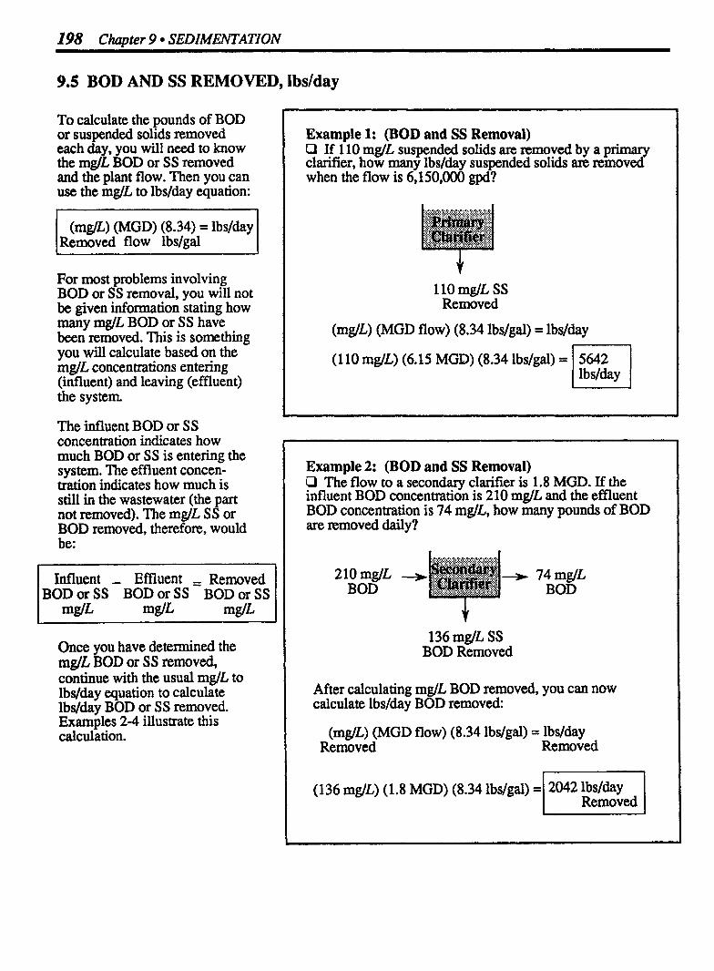
198 Chapter 9 SEDIMENTATION
9.5 BOD AND SS REMOVED, lbslday
To calculate the pounds of BOD or suspended solids removed each day, you will need to know the mglL BOD or SS removed and the plant flow. Then you can use the mg/L to lbslday equation:
I (mg/L) (MGD) (8.34) = lbslday Removed flow lbs/gal
For most problems involving BOD or SS removal, you will not be given information stating how many mg/L BOD or SS have been removed. This is something you will calculate based on the mglL concentrations entering (influent) and leaving (effluent) the system.
The influent BOD or SS concentration indicates how much BOD or SS is entering the system. The effluent concen- tration indicates how much is still in the wastewater (the part not removed). The mglL SS or BOD removed, therefore, would be:
Influent - Effluent = Removed BODorSS BODorSS BODorSS
mg/L mglL
Once you have determined the mglL BOD or SS removed, continue with the usual mglL to lbslday equation to calculate lbs/day BOD or SS removed. Examples 2-4 illustrate this calculation.
Example l: (BOD and SS Removal) D If 110 mglL suspended solids are removed by a primary clarifier, how many lbslday suspended solids an removed when the flow is 6,150,000 gpd?
l l0 mglL SS Removed
(mglL) (MGD flow) (8.34 lbs/gal) = lbs/day
(1 10 mglL) (6.15 MGD) (8.34 lbslgal) =
Example 2: (BOD and SS Removal) P The flow to a secondary clarifier is 1.8 MGD. If the influent BOD concentration is 2 10 mgll, and the effluent BOD concentration is 74 mglL, how many pounds of BOD are removed daily?
210 mg/L -, BOD
Y 136 mglL SS
BOD Removed
After calculating mglL BOD removed, you can now calculate lbs/day BOD removed:
(mglL) (MGD flow) (8.34 lbslgal) = lbslday Removed Removed
(136 mglL) (1.8 MGD) (8.34 lbslgal) = 2042 lbs/da~ / Removed 1
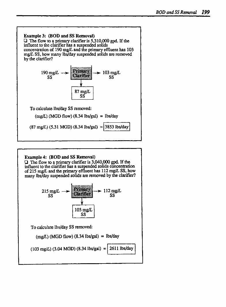
BOD and SS Removal 199
Example 3: (BOD and SS Removal) Q The flow to a primary clarifier is 5,310,000 gpd. If the influent to the clarifier has a suspended solids concentration of 190 mglL and the primary effluent has 103 mg/L SS, how many lbs/&y suspended solids are removed by the clarifier?
To calculate lbslday SS removed:
(mg/L) (MGD flow) (8.34 lbslgal) = lbslday
(87 mglL) (5.31 MGD) (8.34 lbs/gal) = 138531
Example 4: (BOD and SS Removal) P The flow to a primary clarifier is 3,040,000 gpd. If the influent to the clarifier has a suspended solids concentration of 2 15 mglL and the primary effluent has 1 12 mglL SS, how many ibs/day suspended solids are removed by the clarifier?
To calculate lbs/&y SS removed:
(mg/L) (MGD flow) (8.34 lbs/gd) = lbs/&y
(103 mg/L) (3.04 MGD) (8.34 lbs/gal) = 261 l lbs/&y c3

200 Chapter 9 SEDIMEIVZATION
9.6 UNIT PROCESS EFFICIENCY
The efficiency of a treatment process is its effectiveness in removing various constituents from the water or wastewater. Suspended solids and BOD removal are therefore the most common calculations of unit process efficiency.
The efficiency of a clarifier may be affected by such factors as the types of solids in the wastewater, the temperature of the waste- water, and the age of the solids. Typical removal efficiencies for a primary clarifier are as follows:
Settleable Solids----90-99%
Suspended So l id s40 -60%
Total Solids 10-15%
BOD 20-50%
UNIT PROCESS EFFICIENCY IS PERCENT REMOVAL
SS or BOD in influent SS or BOD in effluent (Total SS
SS or BOD Removed
%SS = SS Removed, mglL Removed SS Total, mglL
q, BOD = BOD Removed, mglL X 100
Removed BOD Total, mg/L
Example 1: (Unit Process Efficiency) Q The suspended solids entering a primary clarifier is 182 mglL. If the suspended solids in the primary clarifier effluent is 79 mglL, what is suspended solids removal efficiency of the primary clarifier?
Total Entering 33
103 &L SS Removed
%SS = SS Removed, mglL Removed SS Total, mglL X loo

Unit Process Efficiency 201
Example 2: (Unit Process Efficiency) Cl The influent to a primary clarifier has a BOD concentration of 245 mg/L. If the BOD content of the primary clarifier effluent is 140 mglL, what is the BOD removal efficiency of the primary clarifier?
245 mglL BOD * - 140 mglL
Total Entering BOD
l05 ingL BOD Removed
Example 3: (Unit Process Efficiency) O The suspended solids entering a primary clarif5er is 238 mglL. If the suspended solids in the primary clarifier effluent is 124 mg/L, what is the suspended solids removal efficiency of the primary clarifier?
238 mgfL SS - --p 124 mglL
Total Entering SS
4 114 mglL
SS Removed
% S S = SS Removed, mgL Removed SS Total, mglL


1 0 ?)-ickling Filters
I l. Hydraulic Loading Rate
Primary Ef£lutnt Flow
Recirculated Flow *l I Trickling Filter )
Hydraulic Loading , Total Flow Applied, gpd Rate sqftArea
I (Hydraulic loading rate calcuhtions include recirculatedflws.)
2. Organic Loading Rate
Simplified Equation:
I --p -
agmic Loading BOD, lbslday Rate, -
lbs/day/1000 cu ft - looocuft
Expanded Equation:
(mglL BOD) (MGD) (8.34 ibdgal) 1000 cu ft I

204 Chapter l0 TRICKLING FILTERS
3. BOD and SS Removal, lbdday
BOD or SS Removed (mg/L)
BOD or SS BOD or SS BOD or SS in Influent - in Effluent = Removed
(mglL.) (m*) (m!m
After calculating mglL BOD or SS removed, you can calculate lbs/day BOD or SS removed:
(mp/L) (MGD) (8.34) = lbs/day BOD or SS flow ibdgal BOD or SS Removed Removed
I 4. Unit Process or Overall Efficiency
Unit Process Efficiencv;
SS or BOD , SSorBOD in Influent Trickling Filter in Effluent (Total SS or BOD entering) J.
SS or BOD Removed
%SS = mglL SS Removed hnoved mglL SS Total
S, BOD = mUL BOD Removed 100
knoved mglL BOD Total
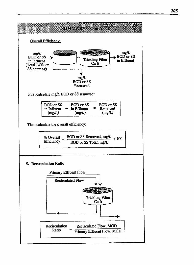
Overall Efficiencv:
m&'.. BOD or SS in Effluent
m%r, BOD or SS Removed
First calculate mg/L BOD or SS removed:
BODorSS BOD or SS - in Effluent = Removed
(m@)
Then calculate the overall efficiency:
% Overall - - BOD or SS Removed, mglL 100 Efficiency BOD or SS Total, mg/L
5. Recirculation Ratio
Primarv Effluent Flow
Recirculated Flow 41 Trickling Filter W
Recirculation Recirculated Flow, MGD Ratio = Primary Effluent Flow, MGD
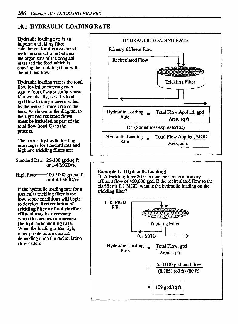
206 Chapter l0 TRICKLING FILTERS
10.1 HYDRAULIC LOADING RATE
Hydraulic loading rate is an important trickling fdter calculation, for it is associated with the contact time between the organisms of the zoogleal mass and the food which is entering the trickling filer with the influent flow.
Hydraulic loading rate is the total flow loaded or entering each squm foot of water surface area. Mathematically, it is the total gpd flow to the process divided by the water surface area of the tank. As shown in the diagnun to the right recirculated flows must be included as part of the total flow (total Q) to the process.
The normal hydraulic loading rate ranges for standard rate and high rate trickling filters are:
Standard Rate-25- 100 gpd/sq ft or 1-4 MGDIac
High Rate -100- 1000 gpd/sq ft or 4-40 MGD/ac
If the hydraulic loading rate for a particular trickling filter is too low, septic conditions will begin to develop. Recirculation of trickling filter or final clarifier effluent may be necessary when this occurs to increase the hydraulic loading rate. When the loading is too high, other problems are created depending upon the recirculation flow pattern.
HYDRAULIC LOADING RATE
Primary Effluent Flow
I Recirculated How J-1
I Trickling Filter 1
Hydraulic Loading = Total Flow Applied, gpd Rate Area, sq ft
pp- p-- -- -
Or (Sometimes expressed as) I 1
Hydraulic Loading = Total Flow Applied, MGD 1 Rate Area, acre
Example 1: (Hydraulic Loading) Q A trickling filter 80 ft in diameter treats a primary effluent flow of 450,000 gpd If the recirculated flow to the clarifier is 0.1 MGD, what is the hydraulic loading on the trickling fdter?
0.45 MGD I----l I P.E.
I Trickling Filter
-L 0.1 MGD
Hydraulic Loading = Total Flow, gpd Rate Area, sq ft
- - 550,000 gpd total flow (0.785) (80 ft) (80 ft)

Hydraulic Loading Rate 207
Example 2: (Hydraulic Loading) P A hi h rate trickling filter receives a flow of 2200 f loading onto the filter?
Pm- If the fi ter has a diameter of 95 ft, what is the hydrau c
(2,200 gpm) (1440 min/day) = 3,168,000 gpd
Hydraulic Loading - - Total Flow, gpd Rate Area, sq ft
- - 3,168,000 gpd (0.785) (95 ft) (95 ft)
Example 3: (Hydraulic Loading) P A hi h rate tricklin filter receives a dail flow of 1.6 a 'E the filter is 90 ft in diameter and 4 fi deep?
L MGD. hat is the hy aulic loading rate in GDIacre if
1.6 MGD 7
(0.785) (90 ft) (90 ft) = 6359 sq ft
First convert sq ft to acres:*
Then calculate hydraulic loading rate:
Hydraulic Loading - - 1.6 MGD Rate 0.146 acres
HYDRAULIC LOADING RATE AS MGDIACRE
Occasionally, the hydraulic loading rate is expressed as MGD per acre. However, this is still an expression of gallons flow over surface area of trickling filter.
* Refer to Chapter 8 in Basic Math Concepts for a discussion of sq ft to acres conversions.

208 Chapter 10 TRICKLING FILTERS
10.2 ORGANIC LOADING RATE
When calculating the lbs/&y BOD entering a wastewater process, you are calculating the organic load on the process-the food entering that process. Organic loading for trickling filters is most often calculated as lbs BODIday per 1000 cu ft media. However, it is sometimes calculated as lbslday BODIper cu ft or lbs BODIday per acre-foot.
In many cases, BOD will be expressed as a mglL concen- tration and must be converted to lbslday BOD,* as shown in the expanded equation.
Note that the "1000" in the denominator of organic loading equations is a unit of measure ("thousand cu ft") and is not part of the numerical calculation.
The normal organic loading rates for standard-rate and high-rate trickling filters are:
dard R a t e 5-25 lbs BOD/&y/1000 cu ft or 200- 1000 lbs BOD/day/ac-ft
Increasing the BOD loading does not have the same effect as increasing the hydraulic loading (which lessens the contact time between the food and organisms and may decnase the efficiency of the trickling filter). To a degree, increasing the BOD loading appears to increase the number of organisms (more food, more organisms).
ORGANIC LOADING RATE
lbs/day BOD -+ Entering
Trickling Filter
Simplified Equation:
Organic bading lbs BODIday I Bate - - loo0 cu ft
Expanded Equation:
Organic Loading @&(L BoD) (MGD) (8.34) Rate
- (0.785) ( D ~ ) (depth, ft)
Organic loading rate is sometimes calculated as:
Organic Loading- lbs BOD/&y Rate -
cu ft
Example l: (Organic Loading Rate) Q A trickling filter 80 ft in diameter with a media depth of 8 ft receives a flow of 950,000 gpd. If the BOD concentration of the primary effluent is 210 mglL, what is the organic loading on the trickling filter in lbs/day/1000 cu ft?
OR
- (2 10 mglL) (0.95 MGD) (8.34 lbs/gal) (0.785) (80 ft) (80 ft) (8 ft)
loo0
Organic Loading- lbs BODIday Rate -
acre-feet
- 1663.83 lbs BODlday 40.192 1000-cu ft
* For a review of mg/L to lbsjday BOD, refer to Chapter 3.

Organic Loadinn Rate 209
Example 2: (Organic Loading Rate) P A 75-ft diameter trickling filter with a media depth of 5 ft receives a primary effluent flow of 3.17 MGD wth a BOD of 107 m& What is the organic loading on the trickling filter in lbs/day/1000 cu ft?
lbslday -1
I Trickling Filter I Cu ft Volum~ (0.785) (75 ft) (75 ft) (5 ft) = 22,078 cu ft
Organic Loading - - lbs BODIday Rate loo0 cu ft
- - (107 mglL) (3.17 MGD) (8.34 lbslgal) 22.1 looecuft
Example 3: (Organic Loading Rate) O A standard rate tricklin filter has a diameter of 100 feet ii and an average media dep of 7 feet. If the 1.2 MGD primary effluent has a BOD concentration of 120 mglL, what is the organic loading in lbs per acre-feet?
Cu ft Volume
= (0.785) (100 ft) (100 ft) (7 ft)
Since organic loading is desired in lbs/&y BOD per acre foot, convert cu ft to acre feet:* (54,950 cu it + 43,560 cu ftlac-ft = 1.26 ac-ft) Now calculate organic loading rate:
Organic Loading - 1201 1bs BOD/&y Rate 1.26 ac-ft
= / 953 lbs BODlday I ac-ft
ORGANIC LOADING RATE AS Ibs BODfdayfac-ft
Although organic loading is most often expressed as lbs BODlday per cu ft or lbs BODlday per loo0 cu ft, it may also be expressed as lbs BODlday per acre-foot. This is still an expression of lbs BODIday per volume.
* For a review of cu ft to ac-ft conversions. refer to Chapter 8 in Bosic Math Concepts.

210 Chapter 10 TRICKLING FILTERS
10.3 BOD AM) SS REMOVED
To calculate the pounds of BOD or suspended solids removed each day, you will need to know the mg/L BOD or SS removed and the plant flow. Then you can use the mg/L to lbs/&y equation:
l (mg/L) (MGD) (8.34) = lbs/day Removed flow lbslgal
BOD AND SS REMOVED
mg/L BOD or SS Removed
First calculate mg/L BOD or SS removed:
BODorSS - BODorSS - - BODorSS in Influent in Effluent Removed
* (mglL) (m@") ( m m
Then calculate lbdday BOD or SS removed:
(mglL) (MGD) (8.34) = lbs/day BOD or SS BOD or SS flow lbs/gal Removed Removed
Example l: (BOD and SS Removal) P If 110 mglL suspended solids are removed by a trickling filter, how many lbs/day suspended solids axe removed when the flow is 4.2 MGD?
(mg/L) (MGD flow) (8.34 lbslgal) = lbslday
* To review mg/L to lbs/day conversions, refer to Chapter 3.

BOD and SS Removal 211
Example 2: (BOD and SS Removal) O The flow to a trickling filter is 4.6 MGD. If the primary effluent has a BOD concentration of 150 mglL and the trickling filter effluent has a BOD concentration of 25 m&, how many pounds of BOD are removed daily?
After calculating mg/L BOD removed, you can calculate lbslday BOD removed:
(mglL) (MGD flow) (8.34 lbdgal) = lbslday Removed Removed
(125 mgL) (4.6 MGD) (8.34 lbslgal) = 4796 lbslday 1 Removed
Example 3: (BOD and SS Removal) O The 3,700,000 d influent flow to a trickling filter has a BOD content of 'it; 5 mglL. If the trickling filter effluent has a BOD content of 68 mg/L, how many pounds of BOD are removed daily?
(mgLL) (MGD flow) (8.34 lbslgal) Removed
= lbslday Removed
(1 17 mglL) (3.7 MGD) (8.34 lbslgal) = ( 3610 lbslday / Removed
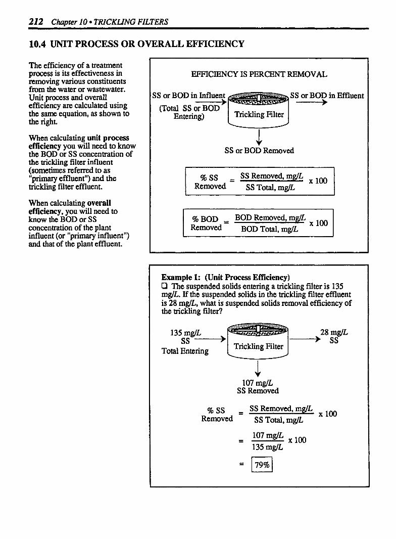
212 Chapter l0 TRICKUNG FILTERS
10.4 UNIT PROCESS OR OVERALL EFFICIENCY
The efficiency of a treatment process is its effectiveness in removing various constituents from the water or wastewater. Unit process and overall efficiency are calculated using the same equation, as shown to the right.
When calculating unit process efficiency you will need to know the BOD or SS concentration of the trickling filter influent (sometimes referred to as "primary effluent") and the trickling fdter effluent.
When calculating overall efficiency, you will need to know the BOD or SS concentration of the plant influent (or "primary influent ") and that of the plant effluent.
EFFICIENCY IS PERCENT REMOVAL
SS or BOD in Influent SS or BOD in Effluent
(Total SS or BOD' _____)
Entering) Trickling Filter
SS or BOD Removed
%SS = SS Removed, mglL b n ~ v e d SS Total, m@
% BOD = BOD Removed, mg/L &xmved BOD Total, mg/L
r lW I
Example 1: (Unit Process Efficiency) P The suspended solids entering a trickling filter is 135 mg/L. If the suspended solids in the trickling filter effluent is 28 mglL, what is suspended solids removal efficiency of the trickling filter?
135 mglL 28 mglL,
Trickling Filter -----+ SS
Total Entering
107 mglL SS Removed
%SS = SS Removed, mglL Removed X 100
SS Total, mglL

Unit Process Eficiency 213
Example 2: (Unit Process Efficiency) P The influent of a primary clarifier has a BOD content of 215 mglL. The trickling filter effluent BOD is 30 m g L What is the BOD removal efficiency of the txeatment ~ lan t?
18s mg/~ SS Removed
%BOD = BOD Removed, mg/L Removed BOD Total, mglL
Example 3: (Unit Process Efficiency) O The BOD concentration of a trickling filter influent is 210 mglL. If the trickling filter effluent flow has a BOD content of 38 m@', what is the BOD removal efficiency of the trickling filter?
210mdL , 38 mg/L BOD -----) BOD
172 mg/L BOD Removed
%BOD = BOD Removed, mg/L Removed BOD Total, mg/L
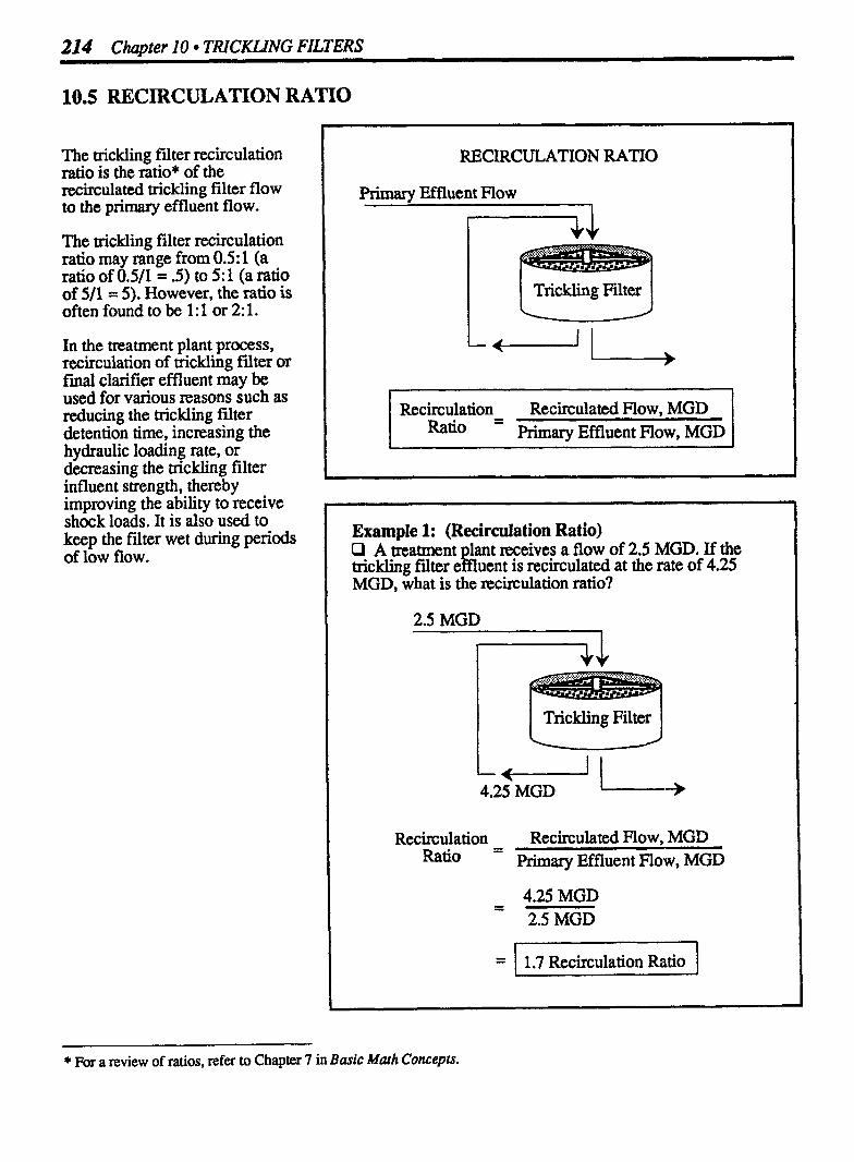
214 Cha~ter 10 TRICKLING FILTERS
10.5 RECIRCULATION RATIO
The trickling filter recirculation ratio is the ratio* of the recirculated trickling filter flow to the primary effluent flow.
The trickling filter recirculation ratio may range from 0.5: 1 (a ratio of 0.5/1 = -5) to 5: 1 (a ratio of 5/1 = 5). However, the ratio is often found to be 1 : 1 or 2: 1.
In the treatment plant process, recirculation of mckling filter or fmal clarifier effluent may be used for various reasons such as reducing the trickling filter detention time, increasing the hydraulic loading rate, or decreasing the trickling filter influent strength, thereby improving the ability to receive shock loads. It is also used to keep the filter wet during periods of low flow.
P P
RECIRCULATION RATIO
Primary Effluent Flow
I I Trickling Filter I
Recirculation - Recirculated Flow, MGD Ratio - Primary Effluent Flow, MGD
Example 1: (Recirculation Ratio) P A treatment lant meives a flow of 2.5 MGD. If the
El trickling filter e uent is recirculated at the rate of 4.25 MGD, what is the ncirculation ratio?
2.5 MGD
I Trickling Filter I
4.25 - MGD _ +
Recirculation - Recirculated Flow, MGD Ratio - Primary Effluent Flow, MGD
- 4.25 MGD 2.5 MGD
= 1 1.7 Recirculation Ratio 1
* For a review of ratios, refer to Chapter 7 in Basic Mufh Concepts.

Recirculation Ratio 215
Example 2: (Recirculation Ratio) P The influent to the trickling filter is 3 MGD. If the recirculated flow is 5.4 MGD, what is the recirculation ratio?
3 MGD 1
I Trickling Filter l
Recirculation - Recirculated Flow, MGD Ratio - Primary Effluent Flow, MGD
- - 5.4 MGD 3 MGD
= 1 1.8 Recirculation Ratio I
Example 3: (Recirculation Ratio) P A trickling filter receives a prim effluent flow of 4 MGD. If the recirculated flow is ~ M G D , what is the recirculation ratio?
4 MGD
I Trickling Filter I
Recirculation - Recirculated Flow, MGD Ratio - Primary Effluent Flow, MGD
- - 4.8 MGD 4 MGD
= I 1.2 Recirculation Ratio I


-
1 1 Rotating Biological Contactors
I 1. Hydraulic Loading Rate
Media Area MGD Flow W ft
Hydraulic Loading = Total Flow Applied, Rate sq ft Area
(Hydraulic loading rate calculations include recirculated flows.)
2. Soluble BOD, mglL
Total BOD = Particulate BOD + Soluble BOD mglL mglL
Obtain from lab (Use K-value* to This is dissolved data convert from BOD
suspended soli& to pm'cul te BOD) T
(SS) (K-valut) = Particulate mglL BOD, mglL
* The K-value for most domestic wastewaters is 0.5-0.7. Although this method allows estimation of soluble BOD, soluble BOD test results are preferred to vsing the K-value approach.

218 Chapter I 1 ROTATING BIOLOGICAL CONTACTORS
Ibs/day BOD -\
sq ft Media
I system Organic Loading = lbdday Soluble BOD I
1OO0 sq ft Total Stages I
I First Stage OrganicLoading = lbs/day Soluble BOD
1000 sq ft First Stage
220 Chapter I I ROTATNG BIOLOGICAL CONTACTORS
11.1 HYDRAULIC LOADING RATE
When calculating the hydraulic loading rate on a rotating biological contactor (RBC), use the sq ft area of the media rather than the sq ft area of the water surface, as in other hydraulic loading calculations. The RBC manufacturer provides media area information.
HYDRAULIC LOADING RATE INCLUDES RECIRCULATED FLOWS
Media Area MGD Flow .Ay J/ sq ft
Hydraulic Loading = Total Flow Applied, gpd Rate Area, sq ft
Example 1: (Hydraulic Loading) P A rotating biological contactor (RBC) treats a primary effluent flow of 1.85 MGD, If the media surface area is 600,000 sq ft, what is the hydraulic loading on the RBC?
Hydraulic Loading - - How, gpd Rate Area, sq ft
- - 1,850,000 gpd 600,000 sq ft
Hydrauric Lwding 221
Example 2: (Hydraulic Loading) C l A rotatin biological contactor treats a flow of 3.6 MGD. f i e manufacturer's data indicates a media surface area of 700,000 sq ft. What is the hydraulic loading rate on the RBC?
Hydraulic Loading - Flow, gpd Rate A=% sq ft
Example 3: (Hydraulic Loading) P A rotatin biological contactor treats a primary effluent flow of 1,278,000 gpd. The manufacturer's data indicates that the media surface area is 500,000 sq ft. What is the hydraulic loading rate on the filter? ,-h
- Media Area
1.27 MGD Flow 500,Ooo sq ft
Hydraulic Loading HOW, & Rate -
Area, sq ft

222 Chapter l l ROTATRVG BIOWGICAL CONTACTORS
11.2 SOLUBLE BOD, mglL
Organic loading on rotating biological contactors is based on lbs/day soluble BOD rather than lbs/day total BOD as in other calcul%ions of organic loading rate. Therefore, in order to calculate the organic loading rate for RBCs, you must first understand how to determine soluble BOD.
The BOD in wastewater can be categorized into two types:
BOD exerted by organic gusoended oartides in the wastewater (particulate BOD), and
BOD exerted by dissolved substances in the wastewater (soluble BOD).
The diagram to the right illus- trates these two components of total BOD.
Many labs do not test for soluble BOD. The BOD test normally conducted is for total BOD. However, there is a method to estimate soluble BOD using the equation shown to the right.*
If you know both total and particulate BOD, you can calculate soluble BOD using the equation shown to the right. Total BOD data is available as lab data. Particulate BOD must be estimated using a K-value.
The K-value indicates how much of the suspended solids is organic suspended solids (i.e., particulate BOD). For most domes tic was tewater, about 50-7096 of the suspended solids are organic suspended solids. (In other words, about 50-70% of the suspended solids are suspended BOD or particulate BOD.) The K-value is normally given as a decimal number rather than a percent (0.5-0.7).
DETERMINING SOLUBLE BOD
Suspended or *OD = Particulate BOD + Soluble BOD
mglL mglL m@
0 b tained from lab data
Use a K-value to convert fiom
suspended solids to
(SS) (K-value) r- Substituting the suspended solids and K-value calculation into the equation above:
Total BOD = (SS) (K-value) + Soluble BOD mglL mglL mglL
Example 1: (Soluble BOD) Q he suspended solids concentration of a wastewater is 260 mglL. If the normal K-value at the plant is 0.5, what is the estimated particulate BOD concentration of the waste- water?
The K-value of 0.5 indicates that about 50% of the suspended solids are organic suspended solids (or "particulate BOD"):
(260 mglL) (0.5) = SS K-value
* Although the K-value method allows estimation of soluble BOD, soluble BOD test results are preferred to using the K-value approach.
Soluble BOD 223
Example 2: (Soluble BOD) O The wastewater entering a rotating biological contactor has a BOD content of 205 mglL. The suspended solids content is 245 mglL. If the K-value is 0.5, what is the estimated soluble BOD (mglL) of the wastewater?
Total BOD = Particulate BOD + Soluble BOD mglL mglL mglL
205 mglL = (245 mglL) (0.5) + X mglL BOD SS Sol, BOD
205 rngl'L = 122.5 mg/L + X mglL Sol. BOD
Example 3: (Soluble BOD) Cl A mating biological contactor receives a flow of 2.3 MGD with a BOD content of 180 mg/L and SS concentra- tion of 150 m& If the K-value is 0.7, how many pounds soluble BOD enter the RBC daily?
Total BOD = Particulate BOD + Soluble BOD mgl ' mglL mglL
180 mglL , (150 mglL) (0.7) + mg/L BOD SS Sol. BOD
180mglL = 105mglL. + X mglL Sol. BOD
Soluble BOD l 7 5 m g K l = x Now lbslday soluble BOD may be determined:
(mglL Sol. BOD) (MGD flow ) (8.34 lbsfgal) = lbs/&y
(75 mglL) (2.3 MGD) (8.341bslgal) =
CALCULATING LBSfDAY SOLUBLE BOD
Once you have determined the soluble BOD in mg/L, you can then determine lbsfday soluble BOD using the mglL to lbs/day equation. *
(MGD) (8.34) = lbs/day flow lbslgal
BOD
* Refer to Chapter 3 for a discussion of mg'L to lbs/day calculations.
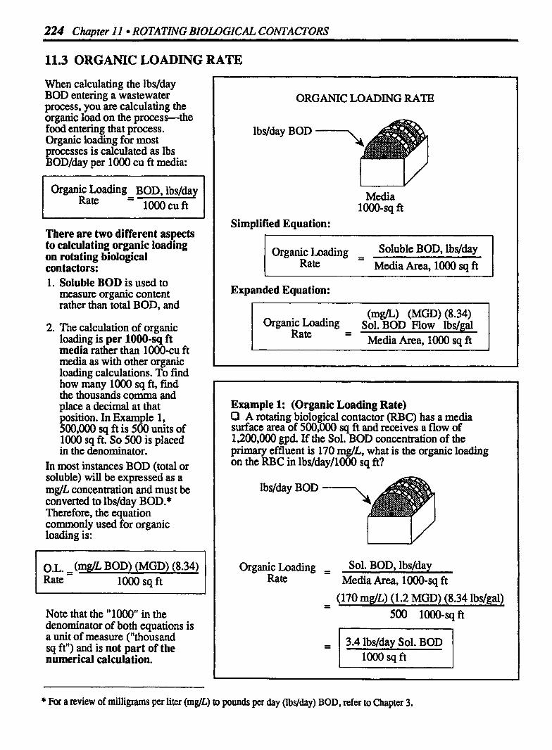
224 Chapter l I ROTATING BIOLOGICAL CONTACTORS
11.3 ORGANIC LOADING RATE
When calculating the lbslday BOD entering a wastewater process, you are calculating the organic load on the process-the food e n t e ~ g that process. Organic loading for most processes is calculated as lbs BOD/&y per loo0 cu ft media:
organic Loading BOD, lbslday Rate -
loo0 cu ft
There are two different aspects to calculating organic loading on rotating biological contactors: 1. Soluble BOD is used to
measure organic content rather than total BOD, and
2. The calculation of organic loading is per 1000-sq ft media rather than 1000-cu ft media as with other organic loading calculations. To find how many 1OOO sq ft, fmd the thousands comma and place a decimal at that position. In Example 1, 500,000 sq ft is 500 units of loo0 sq ft. So 500 is placed in the denominator.
In most instances BOD (total or soluble) will be expressed as a mglL concentration and must be converted to lbslday BOD .* Therefore, the equation commonly used for organic loading is:
Note that the " 1000" in the denominator of both equations is a unit of measure ("thousand sq ft") and is not part of the numerical calculation.
ORGANIC LOADING RATE
Media 1 m s q ft
Simplified Equation:
organic Loading - Soluble BOD, lbslday Rate -
Media Area, 1000 sq ft
Expanded Equation:
Example l: (Organic Loading Rate) O A rotating biological contactor (RBC) has a media surface area of 500,000 sq ft and receives a flow of 1,200,000 gpd. If the Sol. BOD concentration of the primary effluent is 170 mg/L, what is the organic loading on the RBC in lbs/day/1000 sq fi?
lbslday BOD
Organic Loading - - Sol. BOD, lbslday Rate Media Area, 1000-sq ft
- - (170 mglL) (1.2 MGD) (8.34 lbslgal) 500 1000-sqft
= 1 3.4 lbslday Sol. BOD loo0 sq ft
* For a review of milligrams per liter (mg/L) to pounds per day (lbs/day) BOD, refer to Chapter 3.

Organic Loading Rate 225
Example 2: (Organic Loading Rate) P The wastewater flow to an RBC is 3,110,000 gpd. The wastewater has a soluble BOD concentration of 122 mdL. The RBC consists of six shafts (each 100,000 sq ft), with two shafts comprising the Grst stage of the system. What is the organic loading rate lbs/dayl1000 sq ft on the first stage of the system?
Organic Loading - - Sol. BOD, lbslday Rate Media Area, 1OO0 sq ft
- - (122 mglL) (3.1 1 MGD) (8.34 lbdgal) 200 1000-sqft
= 1 15.8 lbs Sol. BOD/day/lOW sq ft I
Example 3: (Organic Loading Rate) 0 A rotatin biolo cal contactor (RBC) receives a flow of 2.4 MGD. &e Bogof the influent wastewater to the RBC is 170 mglL, and the surface area of the mdia is 700,000 sq ft. If the suspended solids concentration of the waste- water is 130 mg/L and the K-value is 0.5, what is the organic loading rate lbslday/lOOO sq ft?
First calculate mglL soluble BOD:
Total BOD , Particulate BOD + Soluble BOD mglL mglL
170 mglL = (130 mglL) (0.5) + X m& BOD SS Sol. BOD
170mglL = 65 mglL + xm& Sol. BOD
105mglL = X 1 Sol. BOD I Then calculate organic loading rate:
Organic Loading = Sol. BOD, lbslday Rate Media Area, 1OOO sq ft
- - (105 mg/L) (2.4 MGD) (8.34 lbs/gal) 700 1000-sq ft
= 1 3 lbs Sol. BOD/day loo0 sq ft
SYSTEM VS. SINGLE STAGE ORGANIC LOADING RATE
Typically, an RBC process includes several shafts of rotating media These shafts are often grouped as "stages". For example, a system comprised of six shafts may have a first stage which includes two shafts. The organic loading rate may be calculated for the entire RBC system or for a single stage.
In Example 1, the organic loading rate was calculated for the entire system. To calculate the organic loading rate for a single stage, include only the sq ft media for that stage. Example 2 illustrates this calculation.


1 2 Activated Sludge
1. Volume-Aera tion Tanks
Volume, cu ft = (length, ft) (width, ft) (depth, ft)
Voluxne-Circular Clarifiers Circular clarifier volume is n o d y calculated using the side wall depth, SWD. (The conkshaped bottom of the tank is not i k l u d )
-
volume, = (Area of Circle, sq ft) (depth, ft) cu ft
I v = (0.785) (D *) (depth ) I
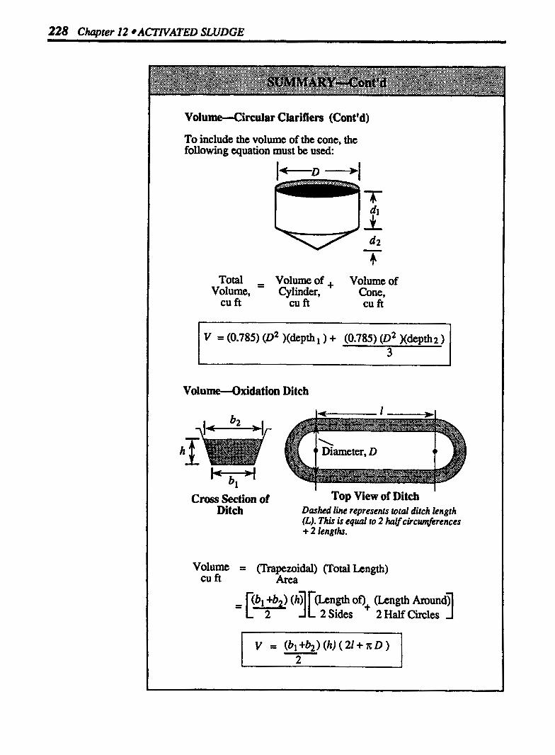
228 Chapter l2 ACTNATED SLUDGE
Volume43 rcular Clarifiers (Cont 'd)
To include the volume of the cone, the following equation must be usad.
Total - Volume of + Volume of Volume, - Cylindtr, Cone,
cu ft cu ft cu ft
Cross Section of Top View of Ditch Ditch Dashed line represents total ditch length
(L). This is equal to 2 halfcircmfirences + 2 lengths.
volume = (Trapezoidal) (Total Length) cu ft Area
of')+ (Length Around) 2 Sides 2 Half Circles l

l 2. BOD or COD Loading, i b s h y
BOD or COD, W h y --&
/ Aeration Tank l/ BOD Loading = (mg/L) (MGD) (8.34) I lbdday BOD flow lbs/gal I COD Loading = (mg/L) (MGD) (8.34) I lbdday COD flow lbs/gal I
I 3. Solids Inventory in the Aeration Tank
I Aeration Tank I /
( To determine the lbs MLSS in the aeration tank:
(mg/L) (Aer. Vol.) (8.34) = lbs MLSS MLSS MG lbs/gal
I To determine the lbs MLVSS in the aeration tank:
(mg/L) (Aer. Vol.) (8.34) (46 Volatile Sol.) = lbs MLVSS MLSS MG 100 1

230 Chapter 12 ACTWATED SLUDGE
4. Food/Microorganism Ratio
BOD or COD,* lbs/day
Ibs MLVSS in Aeration Tank
Simplified Equation:
BOD, lbslday F/M =
MLVSS, Ibs
Expanded Equation:
- -
(m@ BOD) (MGD Flow) (8.34 ibs/gal) = (mglL MLVSS) (Aer Vol. MG) (8.34 Ibslgal)
* COD may be used if there is generally a good correlation in BOD and COD characteristics of the wastewater.
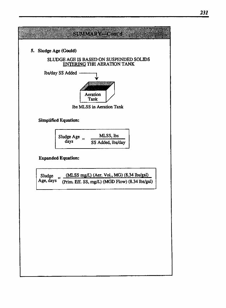
5. Sludge Age (Could)
SLUDGE AGE IS BASED ON SUSPENDED SOLIDS ENTERING THE AERATION TANK
lbs/day SS Added 7
lbs MLSS in Aeration Tank
Simplified Equation:
Sludge Age - - MLSS, lbs days SS Added, lbslday
Expanded Equation:
Sludge - (MLSS mgL) (Aer. Vol., MG) (8.34 lbslgal) Age* &ys - (Prim. Eff. SS, rnglL) (MGD Flow) (8.34 lbslgal)

232 Chapter 12 ACTIVATED SLUDGE
6. Solids Retention Time (SRT) (also called Mean Cell Residence Time, MCRT)
SOLIDS RETENTION TIME IS BASED ON SUSPENDED S O D S LEAVING THE AERATION SYSTEM
P.E. Flow
ving)
(SS leaving)
A RAS Flow .l
Simplified Equation:
WAS Flow
Solids Retention - - Suspended Solids in System, lbs Time, days Suspended Solids Leaving System, lbslday
Solids Retention , - Suspended Solids in System, Ibs Time, days WAS SS, lbslday + S E. SS, lbslday
Expanded Equation:*
(MISS ) (Aer. Vol. ) (8.34 ) + (CCSS ) (Fin. Clar. Vol.) (8.34) SRT, = m& MG lbs/gal mg/L MG lbdgal days (WAS SS) ( WAS Flow) (8.34) + (S.E. SS) (Plant Flow) (8.34)
m& MGD lbslgal mg/L MGD lbslgal
Note: There are four ways to account for system solids (represented by the numerator of the SRT equation). The most accurate calculation of system solids is given in the SRT equation above. The other three methods are described in Section 12.6 of this chapter.
CCSS is the average clarifier core SS concentration of the entire water column sampled by a core sampler.

7. Return Sludge Rate -Using Settleability
(Approximation of Settleorneter RAS flow, R)
The ratio of RAS flow to secondary influent flow can be estimated using the following equation:
R - - - Settled Sludge Volume, mVL Q loo0 ml/L - Settled Sludge Volume, ml/L
The WAS ratio can then be used to calculate RAS flow rate in MGD:
M S Flow Rate, MGD Q Secondary Influent Flow Rate, MGD
Return Sludge Rate - Using Secondary Clarifier Solids Balance
Simplified Equation:
Suspended Solids In = Suspended Solids Out
Expanded Equation:
Suspended Solids In, lbdday Suspended Solids Out, lbs/day* d F I r F -..I I L ( a s s ) (Q + R) 1 (8-34) = L (RAs SS) (R) + (WAS SS) (W)] (8.34) + lbs/gal
! ! lbs/gal
Solids entering from Solids leaving via Solids leaving via the aeration tank the RAS flow the WASflow
Where:
MLSS = mixed liquor suspended solids, mg/L WAS SS = waste activated sludge SS, mg/L Q = secondary influent flow, MGD W = waste sludge flow, MGD R = retm sludge flow, MGD R = return sludge flow, MGD RAS S S = return activated sludge SS, mg/L

234 Chapter I2 ACTNATED SLUDGE
Return Sludge Rate - Using Aeration Tank Solids Balance
Simplified Equation:
Suspended Solids In = Suspended Solids Out * Expanded Equation:**
Suspended Solids h, lbs/day Suspended Solids Out, lbs/&y I
The equation may be rearranged so that both R terms are on the same side of the equation. (Note that since the 834 factor is on both sides of the equation, it can be divided out.)
8. Wasting Rate--Using Constant F/M Ratio
Use the desired F/M ratio and BOD or COD applied (food) to calculate the desired lbs MLVSS:
- Desired lbs MLVSS I
Then determine the desired lbs MLSS using % volatile solids:
Desired - Desired lbs MLVSS MLSS,
- Ibs
% vs 100
Compare the actual and desired MLSS to determine lbs SS to be wasted:
Actual Desired - lbs SS to be lbs MLSS Ibs MLSS - Wasted
* For the aeration tank, this is true only when new cell growth in the tank is considezed negligible. ** Abbreviation of terms is the same as that given for the secondary clarifier solids balance equation.


236 Chapter 12 ACTIVATED SLUDGE
9. WAS Pumping Rate - Using the mdL to Iblday equation
(m@) (MGD) (8.34) = lbslday flow lbslgal
RASSS I Dry Suspended or WAS SS Solids Wasted
When the WAS pumping rate has been calculated in MGD, it can then be easily converted to gpm pumping rate:
(Pumping) (694 gpm/MGD) = Pumping rate, MGD rate, gpm
If the WAS pumping rate in MGD is fmt written as gpd, it may be converted to gprn as follows:
Pumping rate, gpd Pumping - 1440 min/day rate, gpm
WAS Pumping Rate - Using the SRT Equation*
(MISS ) (Aer. Vol. ) 8.34 ). + (CCSS ) (Fin. Clar. Vol.) (8.34 m@
SRT = MO ibslgal m@ MG lbslg
(WAS SS) ( WAS Flow) (8.34) + (S .E. SS) (Plant Flow) (8.34) J
m& MGD lbs/gal m@ MGD lbs/gal
WAS Pumping Rate
CCSS is the avaage clarifier core SS concentration of the entire water column sampled by a core sampler.

I 10. Oxidation Ditch Detention Time
Flow Through
Oxidation Ditch (Top View)
Detention - - Volume, gal Time, Flow, g m
NOTES:
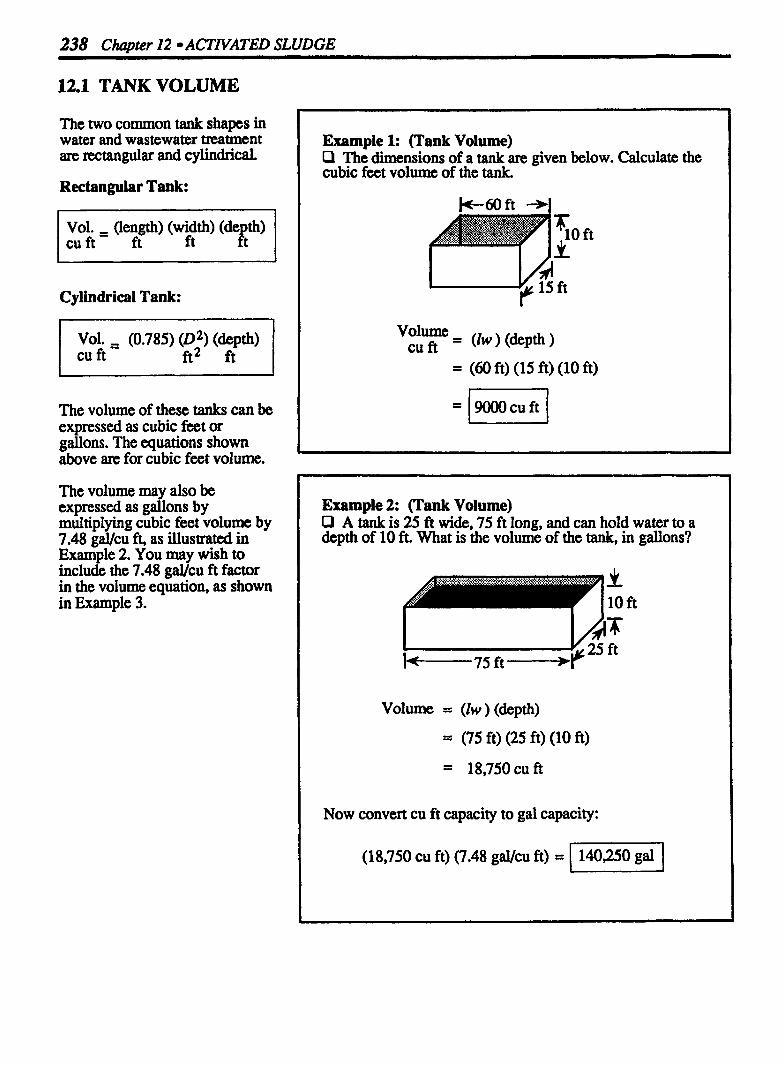
238 Chapter 12 ACTNATED SLUDGE
12.1 TANK VOLUME
The two common tank shapes in water and wastewater treatment are rectangular and cylindrical.
Rectangular Tank:
Vol. , (length) (width) (de th) ft ft Ft
Cylindrical Tank:
Vol. , (0.785) (D 2, (depth) cuft- ft2 ft
The volume of these tanks can be expressed as cubic fcet or gallons. The equations shown above are for cubic feet volume.
The volume may also be expressed as gallons by multiplying cubic feet volume by 7.48 gal/cu ft, as illustrated in Example 2. You may wish to include the 7.48 gucu ft factor in the volume equation, as shown in Example 3.
Example 1: (Tank Volume) 0 The dimensions of a tank are given below. Calculate the cubic feet volume of the tank.
volume = (lw ) (depth ) cu ft = (60 ft) (15 ft) (10 ft)
Example 2: (Tank Volume) Q A tank is 25 ft wide, 75 ft long, and can hold water to a depth of 10 ft. What is the volume of the tank, in gallons?
Volume = (lw ) (depth)
= (75 ft) (25 ft) (10 ft)
= 18,750 cu ft
Now convert cu ft capacity to gal capacity:
(18,750 cu ft) (7.48 gacu ft) = -1
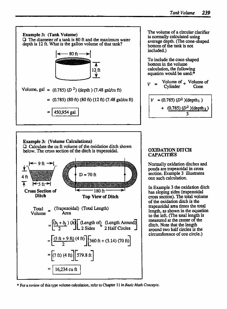
Example 3: (Tank Volume) Q The diameter of a tank is 80 ft and the maximum water depth is 12 ft. What is the gallon volume of that tank?
Volume, gal = (0.785) (D *) (depth ) (7.48 gaVcu ft)
= (0.785) (80 ft) (80 ft) (12 ft) (7.48 gucu ft)
= 1 450,954 gal I
Example 3: (Volume Calculations) Q Calculate the cu ft volume of the oxidation ditch shown below. The cross section of the ditch is trapezoidal.
Cross Section of Ditch Top View of Ditch
Total = (Trapezoidal) (Total Length) Volume Area
= p ft) (4 f t q k79.8 f;l
The volume of a circular clarifier is normally calculated using average depth. (The cone-shaped bottom of the tank is not included.)
To include the cone-shaped bottom in the volume calculation, the following equation would be used:*
Volume of + Volume of v = Cylinder Cone
OXIDATION DITCH CAPAClTlES
Normally oxidation ditches and ponds are trapezoidal in cross section. Example 3 illustrates one such calculation.
In Example 3 the oxidation ditch has sloping sides (trapezoidal cross section). The total volume of the oxidation ditch is the trapezoidal ana t b s the total length, as shown in the equation to the left. (The total length is measmd at the center of the ditch. Note that the length around two half circles is the circumference of one circle.)
* For a review of this type volume calculation, refer to Chapter 1 1 in Basic Math Concepts.

240 C b t e r l2 ACTNATED SLUDGE
12.2 BOD OR COD LOADING
When calculating BOD ), COD, or SS loading on a treatment system, the following equation is used:
l (mg/L) (MGD) (8.34) = lbslday Conc. flow lbs/gal
P-
Loading on a system is usually calculated as lbs/day. Given the BOD, COD, or SS mglL concentration and flow information, the lbs/day loading may be calculated as demonstrated in Examples 1-4.
BOD, COD AND SS LOADING
lbs/day BOD, COD, o r 7 4
BOD, COD, or SS = (mglL) (MGD) (8.34) Loading, lbslday BOD Flow lbs/gal
COD or SS
Example 1: (Loading Calculations) Q The BOD concentration of the wastewater entering an aerator is 215 mglL. If the flow to the aerator is 1,440,000 gpd, what is the lbslday BOD loading?
lbslday BOD '-4
lbslday = (mg/L) (MGD) (8.34) BOD BOD Flow lbs/gal
= (215 mglL) (1.44 MGD) (8.34 lbs/gal)
= 1 2582 lbsjday I BOD

BOD or COD Loading 241
Example 2: (Loading Calculations) P The flow to an aeration tank is 2850 gpm. If the BOD concentration of the wastewater is 130 mglL, how many pounds of BOD are applied to the aeration tank daily?
I Aeration I/ Tank
First convert the gpm flow to gpd flow:
Then calculate lbslday BOD:
(mglL /BOD) (MGD flow) (8.34 lbslgal) = lbslday
(130 mglL /BOD) (4.104 MGD) (8.34 lbslgal) $ 4450 lbs/dsy I BOD
Example 3: (Loading Calculations) P The flow to an aeration tank is 3400 gpm. If the COD concentration of the wastewater is 120 mg/L, how many pounds of COD are applied to the aeration tank daily?
Before the mg/L to lbslday equation can be used the gpm flow must be expressed as MGD flow:
or = 4.9 MGD
Now use the mg/L equation to calculate lbslday COD:
(mg/L COD) (MGD flow) (8.34 lbslgal) = lbslday
(120 mglL COD) (4.9 MGD) (8.34 lbslgal) =I I
Sometimes flow information is not given in the desired t~ms (MGD flow). When this is the case, convert the given flow rate (such as gpd, gpm, a cfs) to MGD flow.*
* Refer to Chapter 8 in Basic Math Concepts for a review of flow conversions.

242 Chapter 12 ACTIVATED SLUDGE
12.3 SOLIDS INVENTORY IN THE AERATION TANK
In any activated sludge system it is important to control the amount of solids under aeration. The suspended solids in an aeration tank are called Mixed Liquor Suspended Solids (MLSS). To calculate the pounds of solids in the aeration tank, you will need to know the mg/L MLSS concentration and the aeration tank volume. Then lbs MLSS can be calculated as follows:"
(mg/L) (MG) (8.34) = lbs MLSS MLSS Vol lbs/gal
Another important measure of solids in the aeration tank is the amount of volatile suspended solids. ** The volatile solids content of the aeration tank is used as an estimate of the microorganism population in the aeration tank . The Mixed Liquor Volatile Suspended Solids (MLVSS) usually comprises about 70% of the MLSS. The other 30% of the MLSS are fixed (inorganic) solids. To calculate the lbs MLVSS, use the following equation:
(mg/L) (MG) (8.34) = lbs MLVSS MLVSS Vol lbdgal
Example 1: (Solids Inventory in Aeration Tank) P If the mixed liquor suspended solids concentration is 1100 mglL, and the aeration tank has a volume of 525,000 gallons, how many pounds of suspended solids are in the aeration tank?
Vol = 0.525 MG
(mg/L) (MG Vol.) (8.34 lbslgal) = lbs
(1 100 mgLL) (0.525 MO) (8.34 lbslgal) 48 1 6 lbs G
Example 2: (Solids Inventory in Aeration Tank) Q The volume of an aeration tank is 175,000 gallons. If the MLVSS concentration is 3220 mg/L, how many pounds of volatile solids are under aeration?
Vol = 175,000 gal or = 0.175 MG
(3220 mglL) (0.175 MG Vol.) (8.34 lbs/gal) = 47001bs (MLVSS
* To review mg/L to lbs conversions, refer to Chapter 3. * * For a discussion of volatile suspended solids calculations, refer to Chapter 6, "Efficiency and Other Percent Calculations".

Soli& Inventory in the Aeration Tank 243
Example 3: (Solids Inventory in Aeration Tank) P The aeration tank of a conventional activated sludge plant has a mixed liquor volatile suspended solids concentration of 2980 mg/L. If the aeration tank is 100 ft long, 40 wide and has wastewater to a depth of 12 A, how many pounds of MLVSS are under aeration?
Vol = (100 ft) (40 ft) (12 ft) (7.48 gal/cu ft)
= 359,040 gal
or = 0.36 MG
Now calculate lbs MLVSS using the usual equation and fill in the given information:
(2980mdL) (0.36MG)(8.341bs/gal) = 89471bs I MLVSS I Example 4: (Solids Inventory in Aeration Tank) O The aeration tank of a conventional activated sludge plant has a mixed liquor suspended solids concentration of 2833 mg/L. with a volatile solids content of 72%. The aeration tank is 85 ft long, 35 wi& and has wastewater to a &pth of 15 ft. How many pounds of MLVSS m under aeration?
Vol = (85 ft) (35 ft) (15 ft) (7.48 gdcu ft)
= 333,795 gal
or = 0.33 MG
The lbs MLVSS can be calculated as follows:
(2833 mgJL) (0.33 MG) (8.34 lbs/gal) (0.72) = 5614 lbs L1

244 Chapter I2 ACTNATED SLUDGE
12.4 FOOD/MICROORGANISM RATIO
In order for the activated sludge process to operate properly, there must be a balance between food entering the system (as measured by BOD or COD) and micro- organisms in the aeration tank (as measured by the MLVSS). The best F/M ratio for a particular system depends on several factors including the type of activated sludge process and the characteristics of the wastewater entering the system.
COD is sometimes used as the measure of food entering the system. COD may be used if there is generally a good correlation in BOD and COD characteristics of the wastewater. The COD test can be completed in only a few hours compared with 5 days for a BOD test.
Note that the F/M equation is given in two forms-the sim- plified equation and the expanded equation. If BOD or COD data is given in lbsfday and MLVSS data is given in lbs, then the simplified equation should be used. In most instances, however, BOD, COD, and MLVSS data will be given as mglL and the expanded equation will be required.
FOOD SUPPLY (BOD OR COD) AND MICROORGANISMS (MLVSS)
MUST BE IN BALANCE
lbs/day BOD (food) or lbsfday COD*
I (Microorganisms) I/ lbs MLVSS in Aeration Tank
Simplified Equation:
F/M = BOD, lbslday MLVSS, lbs
Expanded Equation:
F M = (m@L BOD) (MGD Flow) (8.34 lbslgal) (mglL MLVSS) (Aer Vol, MG) (8.34 lbslgal)
Example 1: (F/M Ratio) P An activated sludge aeration tank receives a primary effluent flow of 2.42 MGD with a BOD of 170 mglL. The mixed liquor volatile suspended solids is 1980 mglL and the aeration tank volume is 350,000 gallons. What is the current F/M ratio?
Since BOD and MLVSS data are given as mglL, the expanded equation will be used. Note that the 8.34 factor can be divided out of the numerator and denominator:
(m@ BOD) (MGD) (8.34 lbslgal) F/M =
(m& MLVSS) (Aer Vol, MG) (8.34 lbslgal)
F/M = (170 mglL ) (2.42 MGD) @S lbslgal) (1980 mglL ) (0.35 MG) lbslgal)

FIM Ratio 245
Example 2: (F/M Ratio) P The flow to a 0.18-MG oxidation ditch is 300,000 gpd. The BOD concentration of the wastewater is 210 mglL. If the mixed liquor suspended solids is 3800 mglL with a volatile solids content of 68%, what is the F/' ratio?
First calculate the mgfL MLVS S:
(3800mglL) (0.68) = 2584 mglL MLSS Vol. Sol. MLVSS
Then calculate the F/M ratio:
F/M = (mglL BOD) (MGD flow) (8.34 lbslgal) (mglL MLVSS) (Ditch Vol. MG) (8.34 lbslgal)
- - (2 10 mglL ) (0.3 MGD) C&34 lbslgal) (2584 mglL ) (0.18 MGD) C&34 lbslgal)
Example 3: (F/M Ratio) O The desired F/M ratio at a particular activated sludge plant is 0.5 lbs COD11 lb mixed liquor volatile suspended solids. If the 3.6 MGD primary effluent flow has a COD of 165 mglL how many lbs of MLVSS should be maintained in the aeration tank?
F/M = COD, lbslday MLVSS, lbs
Fill in the equation with the known information. Since COD is given as mglL, the lbslday COD must be calculated using the expanded equation.*
0.5 = (1 65 mglL ) (3.6 MGD) (8.34 lbslgal)
x lbs MLVSS
Then solve for the unknown value:**
= 1 9908 lbs MLVSS I
* For a review of mglL to lbs/day calculations, refer to Chapter 3.
WHEN MLVSS IS NOT KNOWN
The denominator of the F/M calculation is the mixed liquor volatile suspended solids (MLVS S) concentration. Sometimes, however, you will not have MLVSS information.
The MLVSS concentration can be calculated if you know the MLSS concentration and, percent volatile solids content:
(MLSS) (% Vol. Sol.) = MLVSS 100 m@
CALCULATING DESIRED LBS MLVSS
The F/M ratio equation can be used to calculate desired pounds of MLVSS, given a desired F/h4 ratio. Use the same F/M equation, fill in the given information, then solve for the unknown value (desired lbs MLVSS), as illustrated in Example 3.
* * To review solving for the unknown value, refer to Chapter 2 in Basic Math Concepts.

246 Chapter 12 ACTNATED SLUDGE
12.5 SLUDGE AGE (GOULD)
Sludge age refers to the average number of days a particle of suspended solids remains under aeration. It is a calculation used to maintain the proper amount of activated sludge in the aeration tank. This calculation is sometimes referred to as Gould Sludge Age so that it is not confused with similar calcula- tions such as Solids Retention Time (or Mean Cell Residence Time).
When considering sludge age, in effect you are asking, "how many days of suspended solids are in the aeration tank?" For example, if 2000 lbs SS enter the aeration tank daily and the aeration tank contains 10,000 lbs of suspended solids, then 5 days of solids are in the aeration tank--a sludge age of 5 days.
Notice the similarity of this calculation to that of detention time-sludge age is solids re- tained calculated using units of lbs and lbslday; detention time is water retained, using units of gal and galltime or cu ft and cu ft/time.
Detention - Volume of Tank, gal - Time, min Flow Rate, gpm
SLUDGE AGE IS BASED ON SUSPENDED SOLIDS ENTERING THE AERATION TANK
lbslday SS Added 7
I Aeration I/ Tank
lbs MLSS in Aeration Tank
Simplified Equation:
MLSS, lbs SS Added, lbslday
Expanded Equation:
Sludge Age - (h+fLSS mgL) (Aer. Vol., MG) (8.34 lbslgal) days (P.E.* SS, rnglL) (Flow MGD) (8.34 lbslgal)
Example 1: (Sludge Age) P A total of 2640 lbslday sus ended solids enter an aeration tank in the primary e P fluent flow. If the aeration tank has a total of 13,700 lbs of mixed liquor suspended solids, what is the sludge age in the aeration tank?
2640 lbslday SS 7
13,700 lbs MLSS
Sludge Age - - MLSS, lbs days SS Added, lbs/day
- 13,700 lbs 2640 lbslday
* PE. refers to primary effluent.

Sludge Age 247
Example 2: (Sludge Age) 0 An aeration tank contains 450,000 gallons of wastewater with a MLSS concentration of 2430 m& If the primary effluent flow is 2.3 MGD with a suspended solids concentration of 105 mglL, what is the sludge age?
lbs/day SS Added '-1
Sludge Age - days
-
I Aeration I/ Tank
lbs MLSS in Aeration Tank
MLSS, lbs SS Added, lbslday (2430 m&) (0.45 MG) (8.34 lbs/gal) (105 mglL) (2.3 MGD) (8.34 lbdgal)
9120 lbs MLSS
Example 3: (Sludge Age) C3 An aeration tank is 80 ft lon ,25 ft wide with wastewater to a depth of 15 ft. ' h e mixed liquor suspended solids concentration is 2640 mglL. If the primary effluent flow is 1.73 MGD with a suspended solids concentration of 85 mglL, what is the sludge age in the aeration tank?
lbs/day SS Added -7
Aerator Volume (80 ft) (25 ft) (15 ft) (7.48 gaVcu ft) = 224,400 gal
= 14.0 days I

248 Chapter l 2 ACTIVATED SLUDGE
USING SLUDGE AGE TOCALCULATE DESIRED MLSS
The sludge age equation may be used to calculate the desired mg/L or pounds of MLSS to be maintained in the aeration tank.
In Examples 1-3, sludge age was the unknown variable. However, pounds MLSS (the denominator of the simplified sludge age equation) or mglL MLSS (in the denominator of the expanded sludge age equation) can also be the unknown variable. Examples 4 - 7 illustrate this type of calculation.
Example 4: (Sludge Age) P An oxidation ditch has a volume of 190,000 gallons. The 220,000-gpd flow to the oxidation ditch has a suspended solids concentration of 210 mglL. If the MLSS concentration is 3900 mg/L, what is the sludge age in the oxidation ditch?
lbslday SS Added -7
lbs MLSS
Sludge Age = MLSS, lbs days SS Added, lbslday
(3900 mglL) (0.19 MG) (H4 lbs/gal) (210 mglL) (0.22 MGD) (m lbslgal)
Example 5: (Sludge Age) Ll A slud e age of 5.5 days is desired. Assume 1500 lbslday 'F suspende solids enter the aeration tank in the primary effluent To maintain the desired sludge age, how many lbs of MLSS must be maintained in the aeration tank?
X lbs MLSS
Sludge Age MLSS, lbs days SS Added, lbslday
X lbs MLSS 5.5 days =
l500 lbslday SS Added
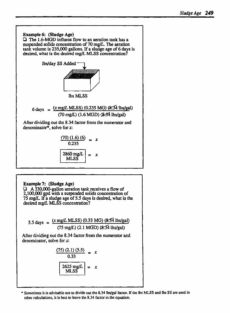
Sludge Age 249
Example 6: (Sludge Age) P The 1.6-MGD influent flow to an aeration tank has a suspended solids concentration of 70 mglL. The aeration tank volume is 235,000 gallons. If a sludge age of 6 days is desired, what is the desired mglL MLSS concentration?
lbs/day SS Added -J
U lbs MLSS
6days = (X mglL MLSS) (0.235 MG) M 4 lbs/gal) (70 mgt'L) (1.6 MGD) (m lbslgal)
After dividing out the 8.34 factor from the numerator and denominator*, solve for X:
2860mglL = X I MLSS I Example 7: (Sludge Age) Cl A 330,000-gallon aeration tank receives a flow of 2,100,000 gpd with a suspended solids concentration of 75 mglL. If a sludge age of 5.5 days is desired, what is the desired mg/L MLSS concentration?
5.5 days = (X m@ MLSS) (0.33 MG) (H4 lbslgal) (75 mg/L) (2.1 MGD) W4 lbslgal)
After dividing out the 8.34 factor from the numerator and denominator, solve for X:
* Sometimes it is advisable not to divide out thc 8.34 lbs/gal factor. If the lbs MLSS and lbs SS are used in other calculations, it is best to leave the 8.34 factor in the equation.

250 Chapter 12 ACTIVATED SLUDGE pp--- - P p- P p - -- P
12.6 SOLIDS RETENTION TIME Solids Retention Time (SRT), also called Mean Cell Residence Time (MCRT), is a calculation very similar to the sludge age calculation. There are two principal differences in calculating SRT: 1. The SRT calculation is
based on suspended solids leaving the system. (Sludge age is based on suspended solids entering the aeration tank.)
2. When calculating lbs MLSS, both the aeration tank and final clarifier volumes are normally used. (In sludge age calculations, only the aeration tank volume is used in calculating lbs MLSS.)
In making SRT calculations, you must determine the pounds suspended solids in the system (solids in the aeration tank and final clarifier). There are actually four different approaches to calculating lbs SS. Each approach results in a slightly different numerator for the SRT equation.
The most accurate method of determining system solids includes a measure of aeration tank solids (mglL MLSS) and a measure of final clarifier solids (mglL SS determined by a core sampler). This first method is given as the "expanded equa- tion", shown to the right.
SOLIDS RETENTION TIMJ3 IS BASED ON SUSPENDED SOLIDS LEAVING THE
AERATION SYSTEM.
P.E. Flow
--F I 1
RAS Flow
Simplified Equation:
WAS Flow (SS leaving)
Solids Retention = Suspended Solids in System, lbs Time Suspended Solids Leaving System, lbs/&y
Solids Retention = Suspended Solids in System lbs Time WAS SS, lbs/day + SE. SS, lbslday
Expanded Equation:
(MLSS ) (Aer. ) 8.34 ) + (CCSS ) (Fin. Clar.) (8.34) m@ Vol. b g a l m& Vol. lbslgal
CRT* MG MG I &ys (WAS SS) ( WAS) (8.34) + (S.E. SS) (Plant) (8.34) 1
mg/L MGD ibs/gal mg/L Flow lbslgal MGD
OTHER METHODS OF DETERMINING SYSTEM SOLIDS 2. To measure aeration tank solids and estimate clarifier solids:
(MLSS ) @ero Vol.) (8.34) + [MISS m a + RAS SS m a ) (Sludge Blanket Vol.) (8.34) = SS m& MG lbs/day 2 MG lbslgal lbs
3, To measure aeration tank solids and estimate clarifier solids; (MLSS mg/L ) (Aer. Vol., MG + Fin. Clar., MG) (8.34 lbslgd) = lbs MLSS
4. To measure aeration tank solids only (MLSS m&) (Aer. Vol., MG) (8.34 lbslgal) = lbs MLSS
* CCSS is the average clarifier core SS concentration of the entire water column sampled by a core sampler. S.E. is Secondary Effluent.
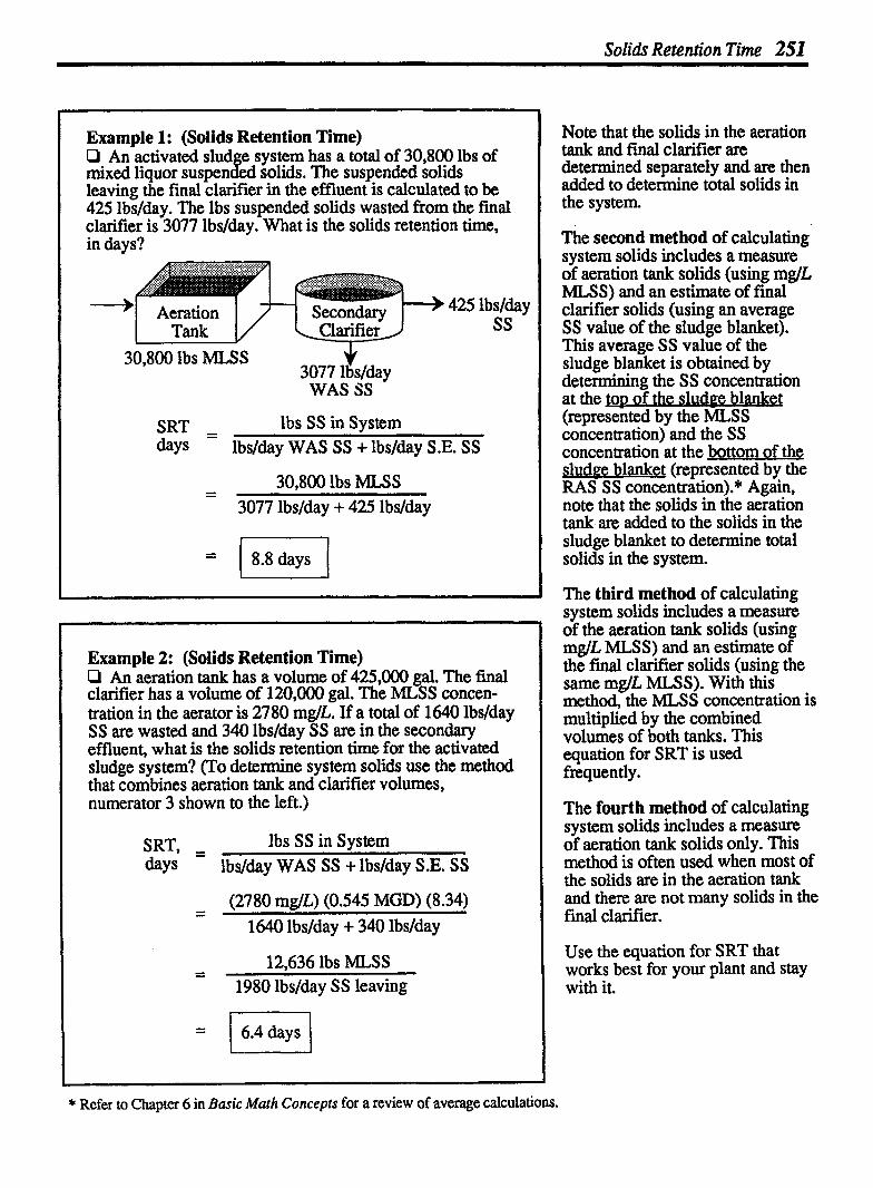
Solidi Retention Time 251
Example 1: (Solids Retention Time) O An activated slud e system has a total of 30,800 lbs of 8 mixed liquor suspen ed solids. The suspended solids leaving the final clarifier in the effluent is calculated to be 425 lbs/day. The lbs suspended solids wasted from the final clarifier is 3077 lbs/day. What is the solids retention time, in days?
-1 Aeration l/- Tank
lbslday SS
30,800 lbs MLSS v 3077 lbs/day WAS SS
SRT - - lbs SS in System days lbs/day WAS SS + lbslday S.E. SS
30.800 lbs MLSS 3077 lbs/day + 425 lbslday
Example 2: (Solids Retention Time) Cl An aeration tank has a volume of 425,000 gal. The final clarifier has a volume of 120,000 gal. The MLSS concen- tration in the aerator is 2780 mglL. If a total of 1640 lbslday SS are wasted and 340 lbslday SS are in the secondary effluent, what is the solids retention time for the activated sludge system? (To determine system solids use the method that combines aeration tank and cider volumes, numerator 3 shown to the left.)
SRT, - - lbs SS in System days lbslday WAS SS + lbslday S.E. SS
(2780 mglL) (0.545 MGD) (8.34) -
1640 lbslday + 340 lbslday
- - 12,636 lbs MLSS 1980 lbs/day SS leaving
= 1 6.4 days 1
Note that the solids in the aeration tank and final clarifier are determined separately and are then added to determine total solids in the system.
The second method of calculating system solids includes a measure of aeration tank solids (using mglL MLSS) and an estimate of final clarifier solids (using an average SS value of the sludge blanket). This average SS value of the sludge blanket is obtained by determining the SS concentration at the top of the sludge blanket (=presented by the MLSS concentration) and the SS concentration at the bottom of the sludge blanket (represented by the RAS SS concentration).* Again, note that the solids in the aeration tank are added to the solids in the sludge blanket to determine total solids in the system.
The third method of calculating system solids includes a measure of the aeration tank solids (using mglL MLSS) and an estimate of the final clarifier solids (using the same mglL MLSS). With this method, the MLSS concentration is multiplied by the combined volumes of both tanks. This equation for SRT is used frequently.
The fourth method of calculating system solids includes a measure of aeration tank solids only. This method is often used when most of the solids are in the aeration tank and there are not many solids in the final clarifier.
Use the equation for SRT that works best for your plant and stay with it.
* Refer to Chapter 6 in Basic Math Concepts for a review of average calculations.

Example 3: (Solids Retention Time) Q Determine the solids retention timc (SRT) given the following data: (Use the equation that includes core sampler suspended solids data, Equation 1 given on the previous page for the SRT numerator.)
Aer. Vol. - 1.5 MG MLSS - 2460 mglL Fin. Clar. Vol. - 0.1 1 MG WAS SS - 8040 mglL P.E. Flow - 3.4 MGD S.E. SS - 18 mg/L WAS Pumping Rate 60,000 gpd CCSS* - 1850 mglL
SRT , SS in System, lbs days SS leaving System, lbs/day
(2460) (1 S ) (8.34) + (1850) (0.1 1) (8.34) = mg/L MG lbslgal mg/L MG lbdgal
(8040) (0.06) (8.34) + (18) (3.4) (8.34) mg/L MGD lbdgal mg/L MGD lbslgal
30,775 lbs MLSS + 1697 1bs CCSS
Example 4: (Solids Retention Time) Cl Calculate the solids retention time (SRT) given the following data: (Use the SRT equation that includes CCSS.) Aer. Vol.- 525,000 gal MLSS -28 10 mglL Fin. Clar. Vol. -120,000 gal WAS SS -6900 mglL P.E. Flow -1.8 MGD S.E. SS -15 mg/L WAS Pumping Rate -24,000 gpd ccss* -1920 m@
S W , - SS in System, lbs days SS Leaving System, lbs/day
(28 10) (0.525) (8.34) + (1920) (0.12) (8.34) mglL MG lbslgal mglL MG lbslgal (6900) (0.024) (8.34)+ (15) (1.8) (8.34) mg/L MGD lbslgal mglL, MGD lbslgal
12,304 lbs MLSS + 1922 lbs CCSS
* CCSS is the average clarifier core SS concentration of the entire water column sampled by a core sampler.

Solids Retention Time 253
Example 5: (Solids Retention Time) P What WAS pumping rate, in MGD, will be re uired
that includes CCS S .) given the information listed below? (Use the SR equation
Aer. Vol.- 355,000 gal MLSS -2340 mkll; Fin. Clar. Vol. -100,000 gal WAS SS -6600 mg/L P.E. Flow -1.7 MGD S.E. SS -16 mglL WAS Pumping Rate -X MGD CCSS -1850 mg/L
Desired SRT - 7 days
___) S.E. SS I Tank W X mgfL MISS 0
WAS SS
SRT - - SS in System, lbs days SS Leaving System, lbslday
First fill in the SRT equation with the known information:
(2340) (0.355) (8.34) + (1850) (0.1) (8.34)
7 days = m& MG ibslgal mglL MG lbslgal
(6600) ( X ) (8.34) + (16) (1.7) (8.34) m@ MGD lbs/gal m& MGD lbs/gal
Next, simplify as many terns as possible before continuing with the calculation:
6928 lbs MLSS + 1543 lbs CCSS 7 days =
(6600) ( X ) (8.34) + 227 lbslday SS *Lr MGD lbslgal
8471 lbs SS 7 days =
(6600) ( X ) (8.34) + 227 lbslday SS mg/L MGD lbslgal
Then solve for the unknown value:*
x = ( 0.0179 MGD I
CALCULATING OTHER UNKNOWN FACTORS
The SRT equation incorporates several variables. In Examples 1-4, SRT was the unknown variable. Other variables can also be the unknown value, as shown below:
Desired MLSS. m@
Desired WAS SS, m@
WAS Pumping Rate, MGD
Regardless of which variable is unknown, use the same SRT equation, fill in the given data, then solve for the unknown value. *
* For a review of solving for the unknown value, refer to Chapter 2 in Basic Math Concepts.

254 Chapter I2 ACTIVATED SLUDGE
12.7 RETURN SLUDGE RATE
RETURN SLUDGE RATE -USING SETTLEABILITY A key aspect in the proper operation of an activated sludge system is maintaining a balance between the food entering the system (measured by BOD or COD) and the microorganisms within that system (measured by the MLSS). Since there is not much control in the amount of food entering the system, most of the control in an activated sludge system is focused on maintaining an adequate solids inventory. One calculation important in this consideration is determination of the return activated sludge (RAS) flow rate.
The most direct method of determining an appropriate return sludge rate is observation of the sludge blanket depth. Depending on whether the sludge blanket depth is rising or falling, the RAS rate is increased or decreased accordingly.
Another method of determining the return sludge rate (RAS pumping rate) is based on the settleability test after 30 minutes.
THE RATIO OF RAS RATE TO INFLUENT FLOW
- (Approximation of Settleorneter RAS flow, R)
The ratio of RAS flow to secondary influent flow can be estimated using the following equation:
R - - - Settled Sludge Volume, ml/L Q looOmVL - SettledSludgeVolume, ml/L
The RAS ratio can then be used to calculate RAS flow rate in MGD:
RAS Flow Rate, MGD Q Secondary Influent Flow Rate, MGD
Example 1: (Return Sludge Rate) O The settleability test after 30 minutes indicates a slud e
R, to the secondary influent flow, Q. Pi settling volume of 210 ml&. Calculate the ratio of RAS ow,
R - Settled Sludge Volume, ml/L Q lOOOml/L-SettledSludgeVolume,xnl/L I - -
W - 210 ml/L Settled Sludge lOOOml/L - 2 1 0 m Set. Sludge

R e m Sludge Rate 255
Example 2: (Return Sludge Rate) Q A total of 280 ml/L sludge settled during a settleability test after 30 minutes. Calculate the ratio of the RAS flow to the secondary influent flow.
R - = ml/L Settled Sludge
Q lOOO-mI/L - W L Settled Sludge
280 mVL Settled Sludge lOOO-mI/L - 280 mJ/L Settled Sludge
Example 3: (Return Sludge Rate) O The secondary influent flow to an aeration tank is 2.95 MGD. If the results of the settleability test after 30 minutes indicate that 3 18 ml/L sludge settled, what is the ratio of the RAS flow to the secondary influent flow? (b) What is the RAS flow expressed in MGD?
(a) R - - - W L Settled Sludge Q 1000-W - ml/L Settled Sludge
318 mVL Settled Sludge - 1000-mVL - 318 ml/L Settled Sludge
(b) R - - - RAS, MGD Q Secondary Influent Flow, MGD
X MGD = 2.95 MGD
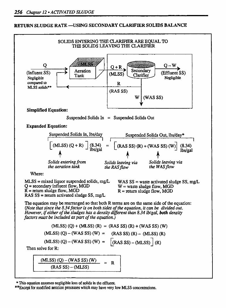
256 C b t e r I2 ACTNATED SLUDGE
RETURN SLUDGE RATE -USING SECONDARY CLARIFIER SOLIDS BALANCE
SOLIDS ENTERENG THE CLARIFIER ARE EQUAL TO THE SOLIDS LEAVING THE CLARIFIER
(Influent S S) Negligible compared to MLSS solids*' I
R
(RAS SS) W (WAS SS)
Simplified Equation: Suspended Solids In = Suspended Solids Out
Expanded Equation:
Suspended Solids In, lbs/day Suspended Solids Out, lbs/day* 1 I-- 7 I r 9 l
Solids entering from soli& leaving via Solids leaving via the aeration tank the RASflow the WASflow
Where:
MLS S = mixed liquor suspended solids, m@ WAS SS = waste activated sludge SS, m@ Q = secondary influent flow, MGD W = waste sludge flow, MGD R = return sludge flow, MGD R = return sludge flow, MGD RAS SS = return activated sludge SS, mg/L
The equation may be rearranged so that both R terms are on the same side of the equation: (Note that since the 8.34 factor is on both sides ofthe equation, it can be divided out. However, if either of the sludges has a dens i~ different than 8.34 lb/gal, both density factors must be included as part of the equation.)
(MLSS) (Q) + (MLSS) (R) = (RAS SS) (R) + (WAS SS) (W)
(MLSS) (Q) - (WAS SS) W) (RAS SS) (R) - (MLSS) (R)
(MLSS) (Q) - ONAS Ss) W) = ERAS s s ) - (MLSS)] (R) Then solve for R:
* This equation assumes negligible loss of solids in the effluent. **Except for modified aeration processes which may have very low MLSS concentrations.
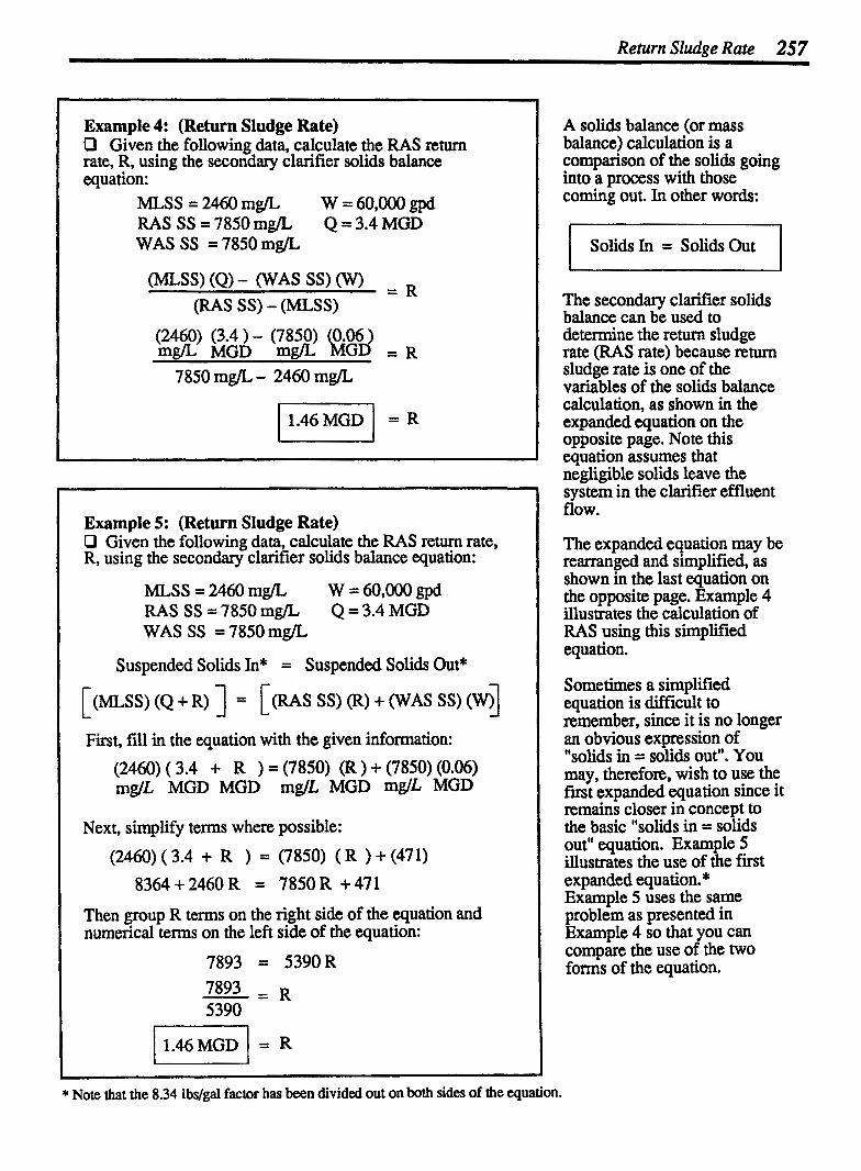
Return Sludge Rate 257
Example 4: (Return Sludge Rate) D Given the following data, calculate the RAS return rate, R, using the secondary clarifier solids balance equation:
MLSS = 2460 m@ W = 60,000 gpd RAS SS = 7850 m& Q = 3.4 MGD WAS SS = 7850 m@
(MLSS) (Q) - (WAS SS) (W) = R
(RAS SS) - (MLSS)
Example 5: (Return Sludge Rate) O Given the following data, calculate the RAS return rate, R, using the secondary clarifier solids balance equation:
MLSS = 2460 mg/L W = 60,000 gpd RAS SS = 7850 m& Q = 3.4 MGD WAS SS = 7850 mgL
Suspended Solids In* = Suspended Solids Out*
First, fill in the equation with the given information:
(2460) ( 3.4 + R ) = (7850) (R ) + (7850) (0.06) mglL MGD MGD mg/L MGD mg/L MGD
Next, simplify terms where possible:
(2460) (3.4 + R ) = (7850) ( R ) + (471)
8364+2460R = 7850R +471
Then group R terms on the right side of the equation and numerical terms on the left side of the equation:
A solids balance (or mass balance) calculation is a comparison of the solids going into a process with those c 0 6 out. In other words:
I Solids In = Solids Out
The secondary clarifier solids balance can be used to determine the return sludge rate (RAS rate) because Eturn sludge rate is one of the variables of the solids balance calculation, as shown in the expanded equation on the opposite page. Note this equation assumes that negligible solids leave the system in the clarifier effluent flow.
The expanded equation may be rearranged and simplified, as shown in the last equation on the opposite page. Example 4 illustrates the calculation of RAS using this simplified equation.
Sometimes a simplified equation is difficult to remember, since it is no longer an obvious expression of "solids in = solids out". You may, therefore, wish to use the first expanded equation since it remains closer in concept to the basic "solids in = solids out" equation. Example 5 illustrates the use of the first expanded equation.* Example 5 uses the same problem as presented in Example 4 so that you can compare the use of the two forms of the equation.
* Note that the 8.34 lbs/gal factor has been divided out on both sides of the equation.

258 Chapter l 2 ACTWATED SLUDGE
RETURN SLUDGE RATE -USING AERATION TANK SOLIDS BALANCE
SOLIDS ENTERING THE AERATION TANK ARE EQUAL TO THE SOLIDS LEAVING THE AERATION TANK
Negligible (InfluentSS) rj Aeration U
Simplified Equation:
compared to MLSS solids** I
Suspended Solids In = Suspended Solids Out*
Expanded Equation:**
R
(RAS SS) W
Suspended Solids In, lbs/da~ Suspended Solids Out, lbs/day I 1 1
(WASSS)
Solidi entering Solids leaving the the aeration tank aeration tank
Where:
MLSS = mixed liquor suspended solids, mg/L R = return sludge flow, MGD Q = secondary influent flow, MGD RAS SS = return activated sludge SS, mg/L
The equation may be rearranged so that both R terms are on the same side of the equation: (Note that since the 834 factor is on both sides of the equation, it can be dropped.)
Then solve for R: h 1
(MLSS) (Q (RAS SS) - (MLSS)
Note that this is the same equation as for the secondary clarifier solids balance except that the aeration tank equation has no WAS term in the numerator (because there is no wasting from the aeration tank), as illustrated in the diagram above.
* For the aeration tank, this is true only when new cell growth in the tank is considered negligible. ** Except for modified aeration processes which may have very low MLSS concentrations.
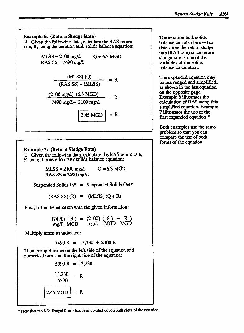
Return Sludge Rate 259
Example 6: (Return Sludge Rate) O Given the followin6 data, calculate the RAS return rate, R, using the aeraoon tank solids balance equation:
MLSS = 2100 mg/L Q = 6.3 MGD RAS SS = 7490 mglL
(2100 mglL) (6.3 MGD) = R
7490 mglL 2100 mglL
Example 7: (Return Sludge Rate) O Given the following data, calculate the RAS return rate, R, using the aeration tank solids balance equation:
MLSS = 2100 mglL Q = 6.3 MGD RAS SS = 7490 mglL
Suspended Solids In* = Suspended Solids Out*
First, fill in the equation with the given information:
(7490) ( R ) = (2100) ( 6.3 + R ) mg/L MGD mglL MGD MGD
Multiply terms as indicated:
Then group R terms on the left side of the equation and numerical terms on the right side of the equation:
5390 R = 13,230
The aeration tank solids balance can also be used to determine the return sludge rate (RAS rate) since nturn sludge rate is one of the variables of the solids balance calculation.
The expanded equation may be rcmanged and simplified, as shown in the last equation on the opposite page. Example 6 illustrates the calculation of RAS using this simplified equation. Exatnple 7 illustrates the use of the first expanded equation.*
Both examples use the same problem so that you can compare the use of both foms of the equation.
* Note that the 8.34 lbs/gal factor has been divided out on both sides of the equation.

260 Chapter 12 ACTNATED SLUDGE
12.8 WASTING RATE
One of the most critical aspects in the operation of an activated sludge treatment system is maintaining a proper balance between the food entering the system (measured by BOD or COD entering) and the microorganisms in the system (measured in a general way by the the mixed liquor suspended solids, MLSS, or more precisely by the mixed liquor volatile suspended solids, MLVSS).
Since there is not much control possible in the amount of food entering the treatment system (the wastewater coming in must be treated), much of th: control of an activated sludge system is focused on controlling (or adjusting) the amount of microorganisms in the system (MLVS S).
The size of the microorganism population naturally increases as food is consumed (measured by BOD or COD removed). Therefore, to maintain the same food-to-microorganism balance, a portion of the microorganism population must be removed or wasted periodically from the system. The question is-how much should be wasted?
Although the microorganism growth rate represents most of the increase in solids within an activated sludge system, another source of solids must also be considered-the suspended solids entering with the primary effluent flow. Wasting rate calculations should consider both sources of solids.
COMPARE DESIRED MLSS WIT33 ACTUAL MLSS TO DETERMINE EXCESS MLSS
Desired MLSS
First calculate desired lbs MLVSS (microorganisms) using the desired FIM ratio and BOD or COD applied @od):
Actual MLSS L
(mg/L) (MG) (8.34) MLSS Aer. Vol. lbs/gal = lbs MLSS
(BOD) (MGD) (8.34) 1 Desired - &,/L- -flow ibs/g& -
Desired lbs MLVSS
Next, determine desired lbs MLSS using % volatile solidr data:
Desired - Desired lbs MLVSS MLSS,
- .. % vs
Then compare the actual and desired MLSS to determine lbs SS to be wasted:
Actual Desired - lbssStobe Wasted 1
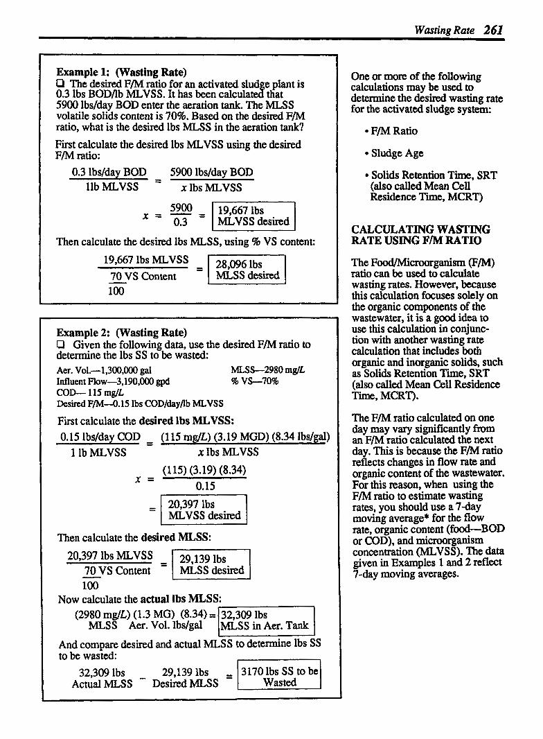
Wasting Rate 261
Example 1: (Wasting Rate) Cl The desired F/M ratio for an activated slud e plant is Ai 0.3 lbs BOD/lb MLVSS. It has been calculat that 5900 lbs/day BOD enter the aeration tank. The MLSS volatile solids content is 70%. Based on the desired F/M ratio, what is the desired lbs MLSS in the aeration tank?
First calculate the desired lbs MLVSS using the desired F/M ratio:
0.3 lbs/dav BOD 5900 lbsldav BOD llb MLVSS
- x lbs MLVSS
X = - - 0.3 MLVSS desired
I
Then calculate the desired lbs MLSS, using % VS content:
Example 2: (Wasting Rate) Q Given the following data, use the desired F/M ratio to determine the lbs SS to be wasted: Aer. Vol.-1,300,000 gal MLSS-2980 mg/L Influent Flow-3,190,000 gpd % VS-70% COD- 115 mg/L Desired FFI-O.15 lbs CODfdayflb MLVSS
First calculate the desired lbs MLVSS: 0.15lbs/dayCOD - - (115mg/L)(3.19MGD)(8.341bs/gal)
1 lb MLVSS x lbs MLVSS
= l 20,397 lbs MLVSS desired
Then calculate the desired MLSS:
70 VS Content MLSS desired
Now calculate the actual lbs MLSS: (2980 mg/L) (1.3 MG) (8.34) =
MLSS Aer. Vol. lbs/gal I I
And compare desired and actual MLSS to determine lbs SS to be wasted: 7
32,309 1bs - 29,139 lbs = / 3170g;lb2 be l Actual MLSS Desired MLSS
One or more of the following calculations may be used to determine the desired wasting rate for the activated sludge system:
F/M Ratio
Sludge Age
Solids Retention Time, SRT (also called Mean Cell Residence Time, MCRT)
CALCULATING WASTING RATE USING F/M RATIO
The Food/Microorganism (FfM) ratio can be used to calculate wasting rates. However, because this calculation focuses solely on the organic components of the wastewater, it is a good idea to use this calculation in conjunc- tion with another wasting rate calculation that includes both organic and inorganic solids, such as Solids Retention Time, SRT (also called Mean Cell Residence Time, MCRT).
The F/M ratio calculated on one day may vary significantly from an F/M ratio calculated the next day. This is because the F/M ratio reflects changes in flow rate and organic content of the was tewater. For this reason, when using the F/M ratio to estimate wasting rates, you should use a 7-day moving average* for the flow rate, organic content (f&BOD or COD), and microorganism concentration (MLVSS). The data given in Examples l and 2 reflect 7-day moving averages.
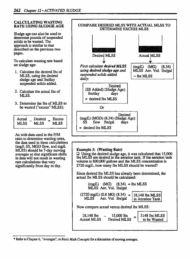
CALCULATING WASTING RATE USING SLUDGE AGE
Sludge age can also be used to determine pounds of suspended solids to be wasted. The approach is similar to that described on the previous two pages.
To calculate wasting rate based on sludge age:
1. Calculate the desired lbs of MLS S, using the desired sludge age and lbs/day suspended solids added.
2. Calculate the actual lbs of MLSS.
3. Determine the lbs of MLSS to be wasted ("excess" MLSS):
Actual - Desired - - Excess MLSS MLSS MLSS
As with data used in the F/M ratio to determine wasting rates, the data used in these calculations (mglL SS, MGD flow, and mglL MLSS) should be 7-day moving averages so that significant shifts in data will not result in wasting rate calculations that vary significantly from day to day.
COMPARE DESIRED MLSS WITH ACTUAL MLSS TO DETERMINE EXCESS MLSS
Desired MLSS Actual MLSS
First calculate desired M W (mg/L) (MG) (8.34) using desired sludge age and MLSS Aer. Vol. lbs/gal suspended solids added = lbs MLSS daily:
Desired (SS Added) (Sludge Age)
lbs/day days I = desired lbs MLSS I
Desired (mglL) (MGD) (8.34) (Sludge Age)
SS flow lbs/gal days I = desired lbs MLSS
Example 3: (Wasting Rate) P Usin the desired slud e age, it was calculated that 15,000 f lbs ML S are desired in t% e aeration tank. If the aeration tank volume is 800,000 gallons and the MLSS concentration is 2720 mglL, how many lbs MLSS should be wasted?
Since desired lbs MLSS has already been determined, the actual lbs MLSS should be calculated:
(mglL) (MG) (8.34) = lbs MLSS MLSS Aer. Vol. lbslgal
1 Now compare actual versus desired lbs MLSS:
(2720 mdL) (0.8 MG) (8-34) = MLss Aer. Vol. lbslgal
18,1481bs - 15,0001bs Actual MLSS Desired MLSS
18,148 lbs MLSS in Aeration Tank
* Refer to Chapter 6, "Averages", in Basic Math Concepts for a discussion of moving averages.

Wasting Rate 263
Example 4: (Wasting Rate) O The desired slud e age for a lant is 4 days. The aeration tank volume is 600, h gpd. If f 000 lbslday suspended solids enter the aeration tank and the MLSS concentration is 2800 m& how many lbs MISS (suspended solids) should be wasted?
First calculate the desired lbs MLSS, using desired sludge age and lbslday SS added:
(3000 lbsfday) (4 days) SS Added Desired '
Sludge Age
Then calculate the actual lbs MLSS:
(mg/L) (MG) (8.34) = lbs MLSS MLSS Aer. Vol. lbs/gal
(2800 mgL) (0.6 MG) (8.34) = MLSS Aer. Vol. lbslgal
And compare desired with actual lbs MLSS :
14,011 1bs - 12,000 lbs 201 1 lbs MLSS Actual MLSS Desired MLSS = I tobewasted I
Example 5: (Wasting Rate) P The desired slud e a e for a lant is 5 days. The aeration tank has a volume 0/75(f000 gz with a MLSS concentration of 2980 mglL. The flow to the aeration tank is 3.9 MGD with a suspended solids concentration of 105 mglL. Calculate the lbs MLSS to be wasted.
First determine the lbs MLSS desired ,using desired sludge age and lbslday SS added:
Then calculate the actual lbs MLSS: i
Now compare actual and desired lbs MLSS:
18,640 lbs - 17,076 lbs 1564 lbs MLSS Actual MLS S Desired MLSS

264 Cha~ter 12. ACTIVATED SLUDGE
CALCULATING WASTING RATE USING SRT
The calculation of lbslday suspended solids to be wasted using the SRT equation is a little different than the previous two methods. Since wasting rate is part of the SRT equation (WAS SS, lbslday), you can leave that factor as the unknown variable* in the SRT calculation and fill in all other terns. Examples 6-8 illustrate this calculation.**
As with the three other methods of wasting rate calculation, the data used in this calculation (MLSS mglL, S.E. SS mglL, and plant flow) should be 7-day moving averages.
USE THE SRT EQUATION TO DETERMINE WASTING RATE
Simplified Equation:
Solids Retention - Suspended Solids in System lbs Time WAS SS, lbslday + S.E. SS, lbs/day
l lbslday SS
Expanded Equation: to be Wasted
(MLSS mg/L) (Aer. + Fin. Clar. Vols., MG) (8.34 lbs/gal) SRT =
WAS SS, lbslday + (S.E. SS) (MGD) (8.34) mdL plant lbslgal
flow I lbslday SS to be Wasted
Example 6: (Wasting Rate) 0 The desired SRT for an activated sludge system is 8.5 days. There are a total of 30,000 lbs SS in the system. The secondary effluent flow has 690 lbs/day suspended solids. To maintain the desired SRT, how many lbsfday suspended solids should be removed?
Write the SRT equation, filling in all information GxceDg WAS SS, lbslday. The simplified equation cm be used in this calculation:
SRT = Suspended Solids in System, lbs WAS SS, lbslday + S.E. SS, lbsjday
8.5 days = 30,000 lbs SS in System x lbslday WAS SS + 690 SS, lbslday
X = 1 2839 lbslday / WAS SS
* For a review of solving for the unknown variable in calculations such as these, refer to Chapter 2 in Basic Math Concepts. ** As described in Section 12.6, the numerator of the SRT equation can be determined using any of four methods. In Section 12.6. the method of determining system solids using core sam~Ier was used primarily. In this discussion the ~ornbined volume method of determining system solids is utilized.

Wasting Rate 265
Example 7: (Wasting Rate) Q The desired SRT for an activated sludge plant is 8 days. There are a total of 28,700 lbs SS in the system. The secondary effluent flow is 3,420,000 gpd, with a suspended solids content of 18 mglL. How many lbslday WAS SS must be wasted to maintain the desired SRT?
Use a modified version of the simplified equation:
8 days = 28,700 lbs SS in System
X lbs/day WAS SS + (18 mglL) (3.42 MGD) (8.34) S.E. SS flow lbslgal
x = 3075 lbslday l WAS SS I
Example 8: (Wasting Rate) Q Given the following data, calculate the lbslday WAS SS to be wasted.
Desired SRT-9 days S.E. SS-16 mglL Clarifier + Aerator Vol.-1.2 MG Inf. Flow- 6.9 MGD
9 days = (3150 mg/L) (1.2 MG) (8.34 lbslgal)
x lbslday WAS SS + (16) (6.9) (8.34) mg/L MGD lbslgd
31,525 lbs SS in System 9 =
X lbslday WAS SS + 921 lbs S.E. SS
X = ( 2582 lbs/day / WAS SS
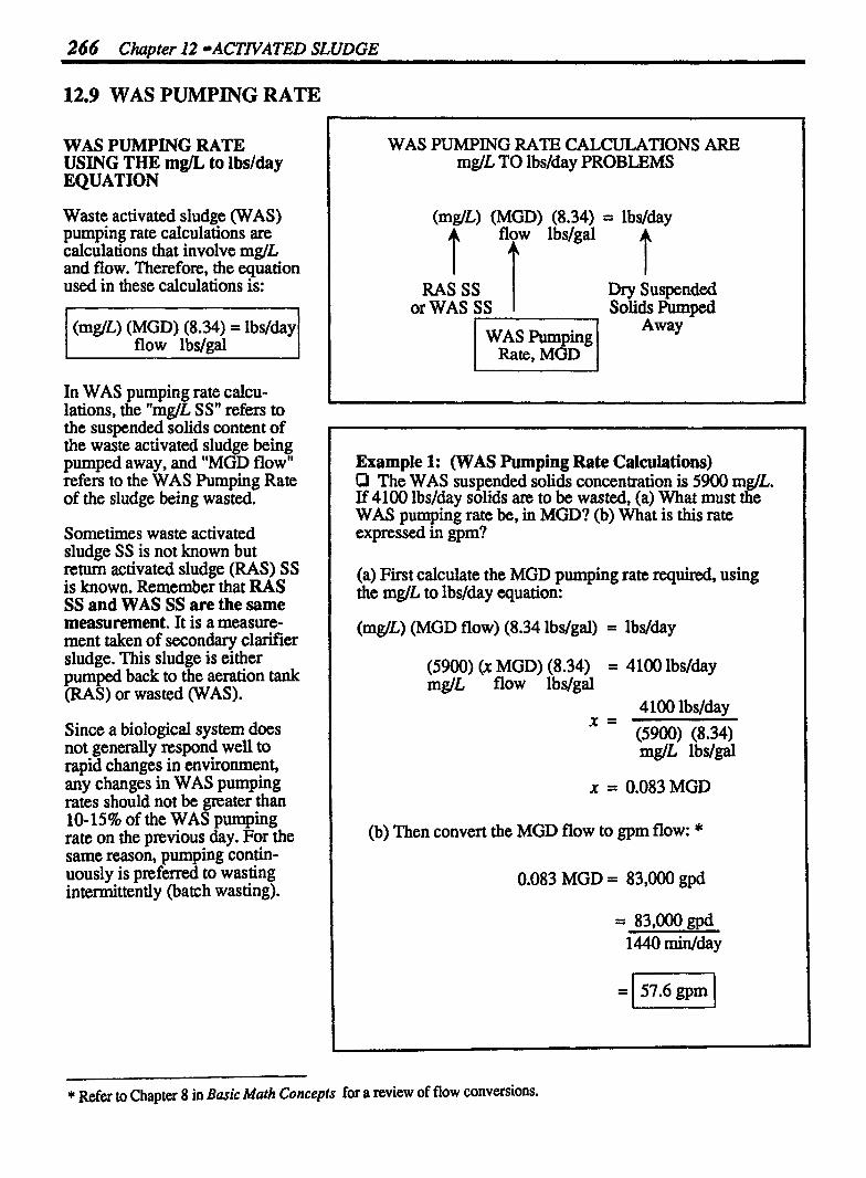
266 Chavter 12 ACTNATED SLUDGE
12.9 WAS PUMPING RATE
WAS PUMPING RATE USING THE m& to lbslday EQUATION
Waste activated sludge (WAS) pumping rate calculations are calculations that involve mglL and flow. Therefore, the equation used in these calculations is:
(m@) (MGD) (8.34) = lbs/day I flowlbdgal
In WAS pumping rate calcu- lations, the "mglL SS" refers to the suspended solids content of the waste activated sludge being pumped away, and "MGD flow" refers to the WAS Pumping Rate of the sludge being wasted.
Sometimes waste activated sludge SS is not known but retum activated sludge (RAS) SS is known. Remember that RAS SS and WAS SS are the same measurement. It is a measure- ment taken of secondary clarifier sludge. This sludge is either pumped back to the aeration tank (RAS) or wasted (WAS).
Since a biological system does not generally respond well to rapid changes in environment, any changes in WAS pumping rates should not be greater than 10- 15% of the WAS pumping rate on the previous day. For the same reason, pumping contin- uously is preferred to wasting intermittently (batch wasting).
WAS PUMPING RATE CALCULATIONS ARE mglL TO lbs/day PROBLEMS
(mg/L) (MGD) (8.34) = lbs/day flow lbs/gal
RAS SS t
Dry Suspended or WAS SS Solids h m ~ e d a
Away
Rate, MGD
Example 1: (WAS Pumping Rate Calculations) Q The WAS suspended solids concentration is 5900 mglL. If 4 1 0 ibs/day solids an to be wasted, (a) What must the WAS pumping rate be, in MGD? (b) What is this rate expressed in gpm?
(a) First calculate the MGD pumping rate required, using the m@ to lbs/&y equation:
(mg/L) (MGD flow) (8.34 lbs/gal) = lbs/&y
(5900) (X MGD) (8.34) = 4100 lbs/&y mgfL flow lbs/gal
X = 0.083 MGD
(b) Then convert the MGD flow to gpm flow: *
0.083 MGD = 83,000 gpd
= 83,000 gpd 1440 min/day
* Refer to Chapter 8 in Basic Math Concepts for a review of flow conversions.

WAS Pumping Rate 267
Example 2: (WAS Pumping Rate Calculations) Cl It has been determined that 5260 lbs/day of solids must be removed from the secondary system. If the RAS SS concentration is 6940 mglL, what must be the WAS pumping rate, in MGD?
Calculate the MGD pumping rate requimk (6940) (X MGD) (8.34) = 5260 lbs/day mglL flow lbs/gal
X = 1 0.0909 MGD I
Example 3: (WAS Pumping Rate Calculations) Q Given the followin data, calculate the WAS pumping rate required (in MGD?: (Use the combined volume method of determining sys tern solids.)
Desired SRT-10 days RAS SS-6290 mglL Clarifier + Aerator Vol.-1.8 MG SoE. S s 1 4 mdL MLSS-27 10 mglL hf. Flow- 4.7 MGD
Use the expanded SRT equation:*
10days = (2710 mglL) (1.8 MG) (8.34 lbs/gal)
(6290 mglL) (X ) (8.34) + (14 mglL) (4.7) (8.34) WAS SS MGD S.E.SS MGD
WAS Flow Plant Flow
- - 40.683 lbs ' - 10 days = (6290) (X MGD) (8.34) + 549 lbs
WAS Pumping Rate
WAS PUMPING RATE USING THE SRT EQUATION
When the lbs/day suspended solids to be wasted is calculated using the F/M ratio or sludge age methods (described in Section 12.8), the WAS pumping rate would be calculated as shown in Examples 1 and 2.
However, when the SRT method is used to determing solids wasting, the WAS pumping rate can be calculated directly, using the SRT equation. (WAS flow, MGD, is the unknown value.) Example 3 illustrates this calculation. To review this method of determining wasting rate, refer to Section 12.8.
review solving for the unknown value for calculations such as these, refer to Chapter Basic Math Concepts.
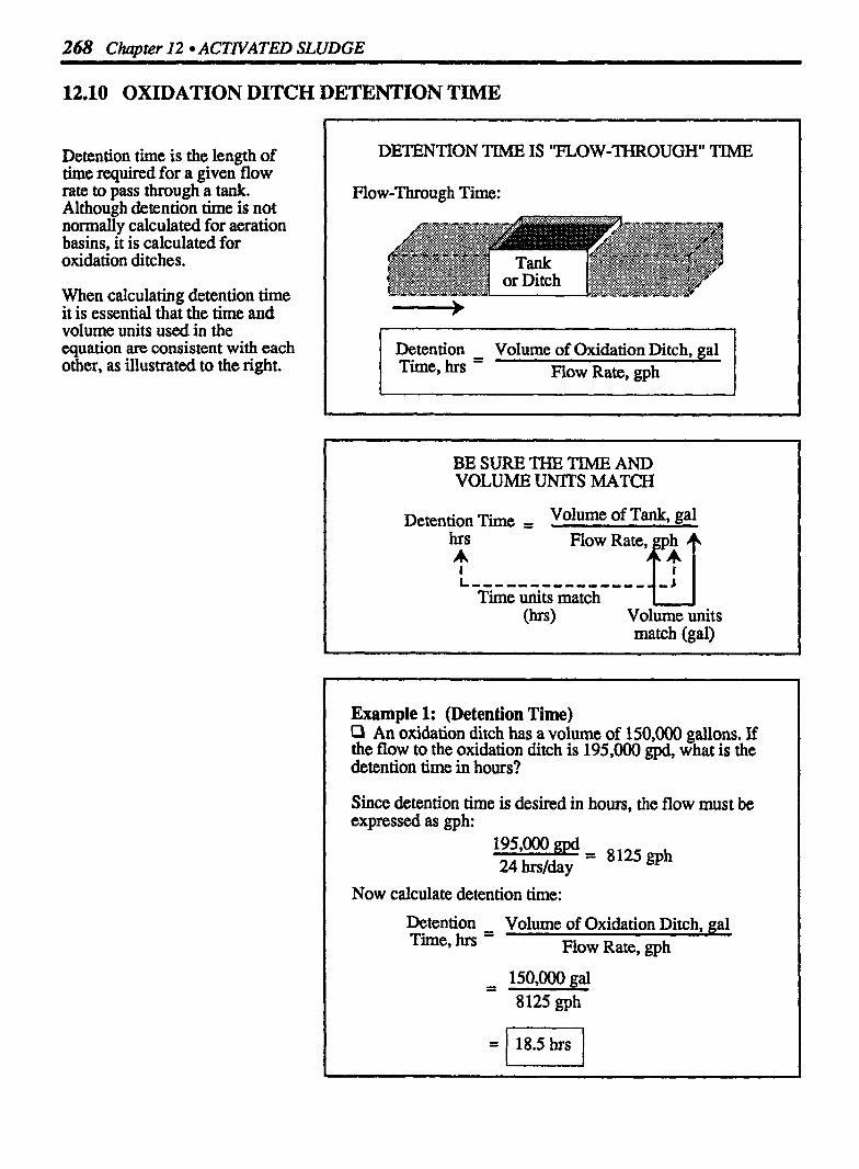
268 Chupter 12 ACTIVATED SLUDGE
12.10 OXIDATION DITCH DETENTION TIME
Detention time is the length of time required for a given flow rate to pass through a tank. Although detention time is not normally calculated for aeration basins, it is calculated for oxidation ditches.
When calculating detention time it is essential that the time and volume units used in the equation are consistent with each other, as illustrated to the right.
- p pp p --
DETENTION TIME IS "FLOW-THROUGH TIME
Flow-Through Time:
Detention - Volume of Oxidation Ditch, gal Time, hrs - Flow Rate, gph
BESIJRETHETIMEAND VOLUME UNITS MATCH
Detention Time = Volume of Tank, gal hrs A I
Time units match (W Volume units
match (gal)
Example 1: (Detention Time) P An oxidation ditch has a volume of 150,000 gallons. If the flow to the oxidation ditch is 195,000 gpd, what is the detention time in hours?
Since detention time is desired in hours, the flow must be expressed as gph:
Now calculate detention time:
Detention - Volume of Oxidation Ditch, gal Time, hrs - Flow Rate, gph
- - lS0,OOO gal 8125 gph
Oxidation Ditch Detention Time 269
Example 2: (Detention Time) O An oxidation ditch receives a flow of 150,000 gpd. If the volume of the oxidation ditch is 138,000 gallons, what is the detention time in hours?
Volume = 138,OOO gal
Detention Time - - Volume of Oxidation Ditch, gal hrs Flow Rate, gph
- - 138,OOO gal Volume 6250 gph
Example 3: (Detention Time) O An oxidation ditch receives a flow of 250,000 gpd. If the volume of the oxidation ditch is l87,OOO gallons, what is the detention time in hours?
Volume = X gal
Detention Time - Volume of Ditch, gal firs Flow Rate, gph
- 187,OOO gal Volume 10,417 gph
-
* Refer to Chapter 8 in Basic Math Concepts for a review of flow rate conversions.

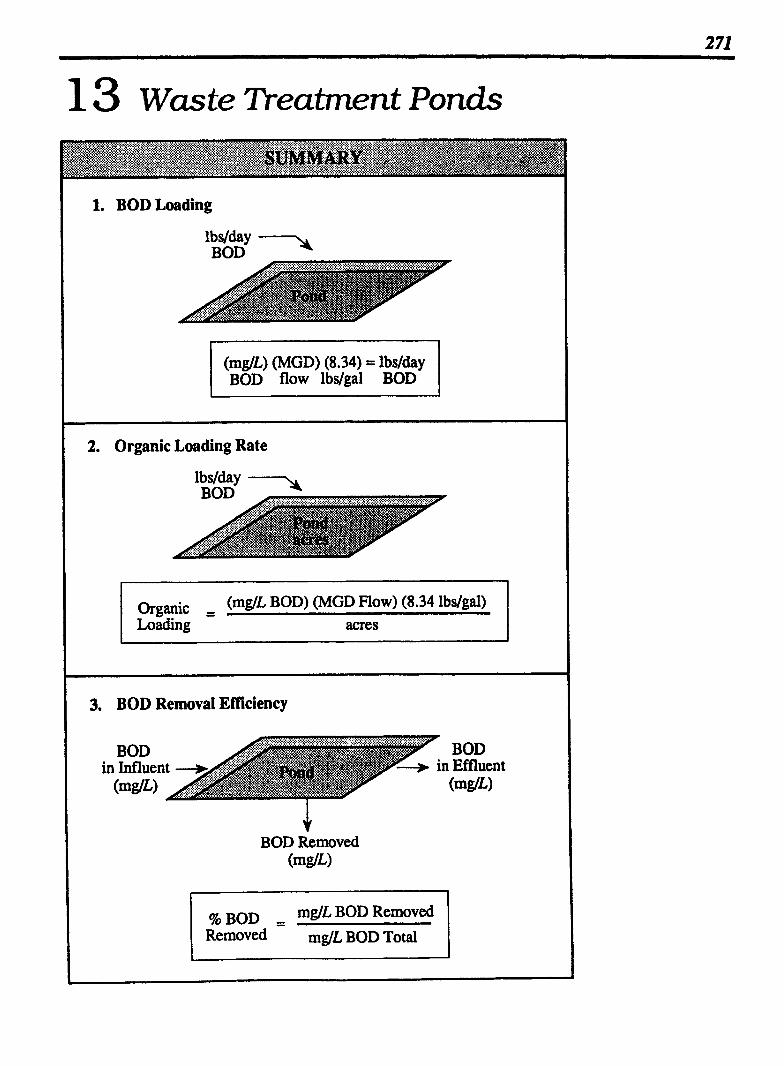
1 3 Waste Tkatrnent Ponds
I 1. BOD Loading
(mg/L) (MGD) (8.34) = lbslday BOD flow lbslgal BOD
1 2. Organic Loading Rate
Organic = (mglL BOD) (MGD How) (8.34 lbdgal) Loading acres
l 3. BOD Removal Eficiency
BOD in Influen (m@")
BOD Removed ( m m
272 Chapter I3 WASTE TREATMENT PONDS d
( 4. Hydraulic Loading Rate Hydraulic loading rate is often calculated as gpdfsq k However the common expression of hydraulic loading rate for ponds is W-ft/day/acre ur inJday.
I sq ft Area
Hydraulic Loading gpd flow Rate 0
sq ft Area
ac Area
Hydraulic Loading W ac-ft/day Rate -
ac
Hydraulic Loading = h- Rate
Population - Persons Loading - acre
5. Population Loading

Detention - Volume of Pond, gal Time, days - Flow Rate, gpd
6. Detention Time Depending on flow data, the detention time can be calculated using either equation shown below.
NOTES:
Detention - Volume of Pond, ac-ft - Flow Rate, ac-ft/day

274 Chapter I3 WASTE TREATMENT PONDS
13.1 BOD LOADING
When calculating BOD loading on a waste treatment pond, the following equation is used:
(mglL) (MGD) (8.34) = lbs/&y BOD flow lbs/gal
Loading on a system is usually calculated as lbslday. Given the BOD concentration and flow information, the lbs/day loading may be calculated as demon- strated in Examples 1-4.
Example 1: (BOD Loading) O Calculate the BOD loadin (lbs/day) on a pond if the influent flow is 0.2 MGD wi t% a BOD of 210 m&
210 m@ -X BOD
(mglL BOD) (MGD flow) (8.34 lbs/gal) = lbslday
(210 mglL) (0.2 MGD) (8.34 Wgal) = 1-1 BOD
Example 2: (BOD Loading) P The BOD concentration of the wastewater entering a pond is 195 mg/L. If the flow to the pond is 180,000 gpd, how many lbs/day BOD enter the pond?
(mglL) (MGD flow) (8.34 lbslgal) = lbslday BOD
(195 rnglL) (0.18 MGD) (8.34 lbslgal) = 293 lbslday 1 BOD I

Example 3: (BOD Loading) Q The flow to a waste treatment pond is 155 m. If the P BOD concentration of the water is 270 mg/L, ow many pounds of BOD are applied to the pond daily?
Before the mg/L to lbs/day equation can be used the gpm flow must be expressed in terms of MGD flow:*
( 1 5 5 H (1440 - rnin) = 223,200 gpd min &Y
or = 0.223 MGD
I Now use the mg/L equation to solve the problem:
I (mg/L) (MGD flow) (8.34 lbslgal) = lbs/day
(270 m@) (0.223 MGD) (8.34 lbs/gal) = 502 lbs/day BOD I BOD I
Example 4: (BOD Loading) O The daily flow to a pond is 310,000 gpd. If the BOD concentration of the wastewater is 410 m&, how many pounds of BOD are applied to the pond daily?
I (mglL) (MGD flow) (8.34 lbs/gal) = lbs/day -
(410 mglL) (0.31 MGD) (8.34 lbs/gal) = 1060 lbs/&y BOD 1 BOD (
Sometimes flow information will not be given in the desired terms (MGD flow). When this is the case, convert the flow rate given (such as gpd, gpm, or cfs) to MGD flow. *
* Refer to Chapter 8 in Basic Math Concepts for a review of flow conversions.

276 Chupter 13 WASTE TREATMENT PONDS
13.2 ORGANIC LOADING RATE
Organic loading rate is a calcu- lation which expresses BOD loading in lbs BOD/day per acre of pond area. Examples 1-3 illustrate this calculation.
ORGANIC LOADING RATE IS BOD LOADING PER ACRE OF POND
Simplified Equation:
Organic = Loading Rate Area, lbSlday acres l
Expanded Equation:
Organic - (mg/L BOD) (MGD Flow) (8.34 lbs/gal) Loading Rate Area, acres
Example 1: (Organic Loading Rate) P A 5.5-acre pond receives a flow of 170,000 gpd. If the influent flow has a BOD content of 160 mglL, what is the organic loading rate on the pond in lbs BOD/day/ac?
5.5-ac Pond
Organic - (160 mg/L BOD) (0.17 MGD) (8.34 lbslgal) Loading Rate - 5.5 ac

Organic Loading Rate 277
Example 2: (Organic Loading Rate) O A 22-acre pond receives a flow of 600,000 gpd. If the influent flow to the pond has a BOD concentranon of 220 mfl , what is the organic loading on the pond in lbs BOD/da y/ac ?
organic - (mgL BOD) (MGD Flow) (8.34 lbs/gal) Loading Rate - ac
- - (220 mglL BOD) (0.6 MGD) (8.34 lbs/gal) 22 ac
Example 3: (Organic Loading Rate) Q A pond has an average width of 380 ft and an average length of 620 ft. The flow to the pond is 121,000 gpd, with a BOD content of 185 mglL. What is the organic loading rate on the pond in lbs BOD/day/ac?
First calculate the pond area, in acres*:
(380 ft) (620 ft) = 235,600 sq ft 235,600 sq ft = 5.4 ac
43,560 sq ftfac
Now continue with the organic loading rate calculation:
Organic - (185 mg/L BOD) (0.121 MGD) (8.34 ibs/gal) Loading Rate - 5.4 ac
- - 1 35 lbs BOD/day ( ac
WHEN POND DIMENSIONS ARE GIVEN
The denominator of the organic loading rate calculation is acres. Therefore, if pond dimensions are given instead of acres, you will need to calculate the sq ft area for the pond and convert sq ft area to acm area.*
* To review the calculation of acres area, refer to Chapter 10 in Basic Math Concepts.

278 Chapter 13 WASTE TREATMENT PONDS
13.3 BOD REMOVAL EFFICIENCY
The efficiency of a treatment process is its effectiveness in removing various constituents from the water or wastewater. BOD removal efficiency is therefore a measure of the effectiveness of the waste txeatment pond in removing BOD from the wastewater.
BOD REMOVAL EFFICIENCY IS PERCENT BOD REMOVED
(Total BOD Entering)
BOD Removed
%BOD = BOD Removed, mgLL &moved BOD Total, mg/L
Example 1: (BOD Removal Efficiency) Q The BOD entering a waste treatment pond is 190 mg/L. If the BOD in the pond effluent is 47 mg/L, what is BOD removal efficiency of the pond?
D Total E
143 mg/L BOD Removed
%BOD = BOD Removed, mg/L Removed BOD Total, mglL

BOD Removal Eflcienqy 279
Example 2: (BOD Removal Efficiency) O The influent of a waste treatment pond has a BOD content of 250 mg/L. If the BOD content of the pond effluent is 70 mglL, what is the BOD removal efficiency of the pond?
0 mglL, BOD
180 mg/L BOD Removed
% BOD = BOD Removed, mglL Removed BOD Total, mglL
Example 3: (BOD Removal Efficiency) Cl The BOD entering a waste treatment pond is 220 mg/L. The BOD concentration of the pond effluent is 44 mglL. What is the BOD removal efficiency of the pond?
220 mglL 44 mglL BOD BOD
176 mglL BOD Removed
%BOD = BOD Removed, mglL Removed BOD Total, mg/L

280 Chapter 13 WASTE TREATMENT PONDS
13.4 HYDRAULIC LOADING RATE
Hydraulic loading rate is a term used to indicate the total flow, in gpd, loaded or entering each square foot of water surface area. It is the total gpd flow to the process divided by the water surface area of the pond. Recir- culated flows must be included as part of the total flow (total Q) to the pond.
When calculating hydraulic loading for wastewater ponds, the answer is often expressed as inJday rather than gpd/sq ft.
There are two ways to calculate inJday hydraulic loading, depending on how the flow to the pond is expressed.
If the flow to the pond is expressed in acre-feetlday:
1. Set up the hydraulic loading equation using acre-ft/day flow per acres area.
2. Canceling terms results in ft/day hydraulic loading.
3. Then convert ft/day to in./day:
( ft ) ( in. ) in. p--- - day ft day
HYDRAULIC LOADING RATE CAN BE CALCULATED USING THREE DIFFERENT
EQUATIONS, DEPENDING ON WHICH DATA IS GIVEN
Influent ,-h -
Hydraulic Loading - Flow, gpd Rate -
Area, sq ft
Hydraulic Loading - Flow, ac-ft/day Rate -
Acre, ac
Hydraulic Loading , i"., Rate day
Example 1: (Hydraulic Loading) P A 25-acre ond receives a flow of 6.2 ac-ft/day. What is P the hydraulic oading on the pond in inJday?
Use the equation for hydraulic loading that uses acre-ft/day flow:
Hydraulic Loading = 6.2 ac-ft/day Rate 25 ac
Then convert ft/day to in./day:

Hydraulic Loading 281
Example 2: (Hydraulic Loading) O A 25-acre ond receives a flow of 5.8 ac-ftfda . What is P 7 the hydraulic oading on the pond in ac-ft/day/ac.
Hydraulic Loading = Flow, gpd Rate Area, sq ft
Example 3: (Hydraulic Loading) Q A waste treatment pond receives a flow of 2,400,000 gpd. If the surface area of the pond is 15 acres, what is the hydraulic loading in in./day?
Area = 15 ac or (15 ac) (43,560 sq ft/ac)
= 653,400 sqft
Hydraulic Loading 2,400,000 gpd Rate - 653,400 sq ft
Convert gpd flow to ft 3/day flow (2,400,000 gpd + 7.48 gUcu ft = 320,856 ft 3/day):
- 320,856 ft 3/day 653,400 ft2
= 0.5 ftlday Then convert to idday:
* For a review of flow conversions, refer to Chapter 8 in Basic Math Concepts.
If the flow to the pond is expressed in gpd:
1. Set up the hydraulic loading equation as gpdfsq ft.
2. Convert gpd flow to cubic feet per day flow (cfd or ft3/day). This is done by dividing gpd by 7.48 gal/cu ft.*
3. Cancel terms to obtain ft/day hydraulic loading. **
f m ~ - - = ft/day sqft f t2
4. Then convert Wday to in./day (by multiplying by 12 inJft).
(Note: There is a shortcut method to determine in.l&y hydraulic loading using the conversion factor of l gpdfsq fr = l .6 in.lday. To use the shortcut method, first calculate the hydraulic loading rate in gpdlsq ft. Then multiply by the conversion factor of 1.6 to obtain hydraulic loading, in.1da-y.)
* * To review cancellation of terms, refer to Chapter IS, "Dimensional Analysis", in Basic Math Concepts.

282 Chapter 13 WASTE TREATMENT PONDS
13.5 POPULATION LOADING AND POPULATION EQUIVALENT
POPULATION LOADING
Population loading is a calcu- lation associated with wastewater tmatment by ponds. Population loading is an indirect measure of both water and solids loading to a system. It is calculated as the number of persons served per acre of pond:
Population - - Persons Loading Acre
Example 1: (Population Loading) O A 3.5-acre wastewater pond serves a population of 1500. What is the popula~on loading on the pond?
Population - - Persons Loading Acre
- - 1500 persons 3.5 acres
429 persons acre
Example 2: (Population Loading) O A wastewater pond serves a po ulation of 4000. If the pond is l6 acres, what is the pop ation loading on the pond?
J
Population - persons Loading acre
- 16 acres

Example 3: (Population Equivalent) O A 0.4-MGD wastewater flow has a BOD concentration of 1800 m@ BOD. Using an average of 0.2 lbs BOD/day/ person, what is the population equivalent of this wastewater flow?
Population - - BOD, Ibslday l bs BODIda y/person
Convert mglL BOD to lbs/day BOD* then divide by 0.2 lbs BOD/day/person:
Population - (1 800 mglL) (0.4 MGD) (8.34 lbslgal) Equivalent - 0.2 lbs BOD/day/person
= 1 30,024 people 1
Example 4: (Population Equivalent) O A 100,000-gpd wastewater flow has a BOD content of 2800 mglL. Using an average of 0.2 lbslday BODIperson, what is the population equivalent of this flow?
Population - - BOD, lbslday lbsBOD/day/person
(2800 mg,L) (0.1 MGD) (8.34 lbslgal) 0.2 lbs BOD/day/person
= 1 1 1,676 people I
POPULATION EQUIVALENT
Industrial or commercial waste- water generally has a higher organic content than domestic wastewater. Population equi- valent calculations equate these concentrated flows with the number of people that would produce a domestic wastewater with that organic load. For a domestic was tewater system, each person served by -the system contributes about 0.17 to 0.2 lbs BOD/day To determine the population equivalent of a wastewater flow, thexefore, divide the lbs BOD/day content by the ibs BOD/day contributed per person (e.g., 0.2 lbs BOD/day).
* For a review of mg/L to lbs/day calculations, refer to Chapter 3.

284 Chupter 13 WASTE TREATMENT PONDS
13.6 DETENTION TIME
There are many possible ways of writing the detention time equa- tion, depending on the time unit desired (seconds, minutes, hours, days) and the expression of volume and flow rate.
When calculating detention time, it is essential that the time and volume units used in thc equation are consistent with each other, as illustrated to the right.
TWO EQUATIONS FOR DETENTION TIME
Flow-Through Time:
Detention - Volume of Pond, gal - Time, days Flow Rate, gpd
Detention - Volume of Pond, ac-ft - Time, days Flow Rate, a c - f a y
BE SURE THE TIME AND VOLUME UNITS MATCH
Detention Time, = Volume of Tank, ac-ft days Flow Rate, ac-ftl
Time units match U (day) Volume units
match (ac-ft)
Example 1: (Detention Time) O A waste treatment ond has a total volume of 25 ac-ft. If the flow to the pon B is 0.58 ac-ftlday, what is the detention time of the pond (days)?
Detention - Volume of Pond, ac-ft - Time, days Flow Rate, ac-ft/day
- - 25 ac-ft 0.58 ac-ft/day

Detention Time 285
Example 2: (Detention Time) Cl A waste treatment pond is operated at a depth of 5 feet. The average width of the pond is 390 ft and the average length is 640 ft. If the flow to the pond is 540,000 gpd, what is the detention time, in days?
(640 ft) (390 ft) (5 ft) (7.48 gaVcu ft) = 9,335,040 gal Volume
Detention Time - - Volume of Pond, gal days Flow Rate, gpd
- 9,335,040 gal Volume 540,000 gpd
Example 3: (Detention Time) Cl A waste treatment ond has an avera e length of 650 ft, P di an average width of 4 0 ft, and a water epth of 4 ft. If the flow to the pond is 0.5 ac-ft/day what is the detention time for the pond in days?
First calculate cu ft volume then ac-ft volume:
(650 ft) (450 ft) (4 ft) = 1,170,000 cu ft
Then calculate detention time:
Detention - - 26.9 ac-ft Time* &YS 0.5 ac-ft/day
= 53.8 days D
CALCULATING ACRE-FEET VOLUME
Occasionally it will be necessary to calculate ac-ft volume of a pond in order to complete a detention time calculation. Once cu ft volume of the pond has been calculated,* ac-ft volume can be determined:
Volume, - Volume, W ft ac-ft 43,560 cu ft/ac ft
* Refer to Chapter l l in Basic Moth Concepts for a discussion of volume.

14 Chemical Dosage
I I
1. Chemical Feed Rate, Ibdday-Full-S trength Chemicals
7
I l (mgL Chem.) (MGD flow) (8.34 lbs/gal) , lbs/day Chemical
2. Chlorine Dose, Demand and Residual
Cl2 Dose = Cl2 Demand + Cl2 Residual
3. Chemical Feed Rate, lbslday-Less Than Full-S trength Chemicals
(mglL Chem.) (MGD flow) (8.34 lbslgal) Ibs,b,, - % Strength of Chemical Chemical
100
(mglL Chem.) (MG Tank Vol.) (8.34 lbs/gal) - lbs/&,, - % Strength of Chemical Chemical
1 4. Percent Strength of Solutions
l Percent strenmh using dry chemicals:
% Strength = Chemical, lbs , Solution, lbs
l percent strewth using liauid chemicals;
(Liquid Polymer) (% Stmgth) = (Polymer Solution) (%Strength) lbs of Liq. Poly . lbs of Poly. Soln.
100 100
288 Chapter 14 CHEMICAL DOSAGE
5. Mixing Solutions of Different Strength
% Sangth , lbs Chemical in M i x w of Mixture lbs Solution Mixture
Q& if target strength is desired: Higher 8 Sol'n Parts Higher % S o h
Lower % S o h Parts Lower % Sol'n
6. Solution Chemical Feeder Setting, gpd
Simplified Equation:
Desired Dose = Actual Dose lbsfday lbs/day
I Expanded Eouation:
(mg/L) (MGD Flow) (8.34) = (mglL) (MGD) (8.34) Dose Treated lbs/day Sol'n S o h lbs/gal
1 7. Chemical Feed Pump-% Stroke Setting
% Setting = Required Feed Pump, gpd Maximum Feed Pump, gpd

8. Solution Chemical Feeder Setting, W m i n
First calculate solution flow reauired;
Simplified Equation;
I Desired Dose, lbslday = Actual Dose, lbslday I Expanded Equation:
(mgl..) (MGD) (8.34) = (mg/L) (MGD) (8.34) Dose Flow lbs/gal S o h S o h lbs/gal
Treated Flow
Then convert W m i n solution flow rea-uired:
9. Dry Chemical Feeder Calibration
Chemical Feed , - Chemical Used, lbs Rate, lbslday Application Time, days
10. Solution Chemical Feeder Calibration (Given mL/rnin Flow)
First convert rn~lmin flow to p d flow:
Then calculate chemical dosape. lbsldav:
(mg/L Chem.) (MGD flow) (8.34 ibslgal) = chemical, lbs/day

290 Chapter 14 CHEMICAL DOSAGE
11. Solution Chemical Feeder Calibration (Given Drop in Solution Tank Level)
Diameter
Drop in J. solution Level, ft
How , Volume Pumped, gal gpm Duration of Test, min
Flow , - (0.785) (02) (Drop, fi) (7.48 g a b ft)
g . m Duration of Test, min
12. Average Use Calculations
First determine the average chemical use;
Average use - Total Chem. Used, lbs I 1bsld.y -
Number of Days
Average Use - - Total Chem. Used, gal Number of Days
Then calculate day's sup~lv in inventorv
Day's Supply - - Total Chea in InventoryJbs in Inventory Average Use, lbslday
Day's Supply = Total Chem. in Inventory, g in Inventory Average Use, gpd

292 Chapter I4 CHEMICAL DOSAGE
14.1 CHEMICAL FEED RATE-Qosing Full-Strength Chemicals)
In chemical dosing, a measured amount of chemical is added to the water or wastewater. The amount of chemical required depends on such factors as the type of chemical used, the reason for dosing, and the flow rate being treated.
The two expressions most often used to describe the amount of chlorine added or required are:
milligrams per liter (mglL)*, and
pounds per day (lbslday)
CHLORINE DOSAGE
Was tewater may be chlorinated during various stages of treatment. For example, chlorination in the early stages of treatment may be practiced for odor control. In other cases, chlorination may be used to aid in grease removal or BOD reduction. In the chlorination of secondary effluent, disinfection is the principal objective. Chlorine is added to kill the disease-causing organisms which are a potential health hazard if discharged into receiving waters used for human consumption or water contact sports such as swimming.
MILLIGRAMS PER LITER IS A MEASURE OF CONCENTRATION
Assume each liter below is divided into 1 million parts:
4 mg/L solids
- 8 mglL - solids
1 liter 1 liter = l,OOO,OOO mg = l,OOO,OOO mg
The mglL concentration expresses a ratio of the milligrams chemical in each liter of water. For example, if a concentration of 4 mglL is desired, then a total of 12 mg chemical would be required to treat 3 liters:
The amount of chlorine required therefore depends on two factors:
.The desired concentration (mglL), and The amount of water to be treated (normally expressed as MGD).
To convert from mglL to lbs/day, the following equation is used:
(mglL) (MGD) (8.34 ) Chem. flow lbslgal = lbslday
* For most water and wastewater calculations, mglL concentration and ppm concentration may be used interchangeably. That is, 1 mg/L = 1 ppm. Of the two expressions, mg/L is preferred.

Chemical Feed Rate 293
Example 1: (Chemical Feed Rate) P Determine the chlorinator setting (lbslday) needed to treat a flow of 3 MGD with a chlonne dose of 4 m&.
First write the equation. Then fd in the information given:
(mglL Cl2) (MGD flow) (8.34 lbs/gal) = lbs/day Cl2
(4 m@ Cl2) (3 MGD) (8.34 lbs/gal) = 1 100 lbs/&y cl2 1
Example 2: (Chemical Feed Rate) O The desired dosage for a dry polymer is 12 m& If the flow to be treated is 2,160,000 gpd, how many lbs/day polymer will be required?
(mglL Chem.) (MGD flow) (8.34 lbs/day ) = lbs/day Polymer
(12 mglL Polymer) (2.16 MGD) (8.34 lbs/day) =
Example 3: (Chemical Feet Rate) C3 To neutralize a sour digester, one und of lime is to be 8" added for every pound of volatile aci S in the digester sludge. If the digester contains 250,000 gal of sludge with a volatile acid (VA) level of 2,300 mglL, how many pounds of lime should be M?
Since the VA concentration is 2300 mglL, the lime concentration should also be 2300 mglL:
(mglL) (MO) (8.34) = lbs Lime Lime Dig.Vo1 lbs/gal Required
DOSAGE OF OTHER CHEMICALS
When calculating the dosage rate for other chemicals such as alum, polymer, or lime, the same equation is used as for chlorine dosage.
DOSAGE IN A TANK
To calculate chemical dose for tanks or pipelines, a slightly modified equation must be used. Instead of MGD flow, MG volume is used:
(mglL ) (MG) (8.34) = lbs Chem. Tank lbs/gal Chem.
Vol.

294 Chapter 14 CHEMICAL DOSAGE
14.2 CHLORINE DOSE, DEMAND AND RESIDUAL
CHLORINE DOSAGE, DEMAND, AND RESIDUAL
In some chlorination calcula- tions, the mg/L chlorine dose is not given directly but indirectly as chlorine demand and residual information.
Chlorine dose depends on two considerations-the chlorine demand and the desifed chlorine residual:
Dose = Demand + Resid. mg/L mg/L
The chlorine demand is the amount of chlorine used in reacting with various compon- ents of the water such as harmful organisms and other organic and inorganic substances. When the chlorine demand has been satisfied, these reactions stop.
In some cases, such as perhaps during pretreatment, chlorinating just to meet the chlorine demand is sufficient. In other cases, however, it is desirable to have an additional amount of chlorine in the water available for disinfection.
Example 1: (Chlorine Dose, Demand, Residual) Q The secondary effluent is tested and found to have a chlorine demand of 6 mg/L. If the desired chlorine residual is 0.8 mglL, what is the desired chlorine dose in mg/L?
C1 2 Dose I
Example 2: (Chlorine Dose, Demand, Residual) O The chlorine demand of a secondary effluent is 9.5 mglL. If a chlorine residual of 0.6 mglL is desired, what is the desired chlorine dosage in mg/L?
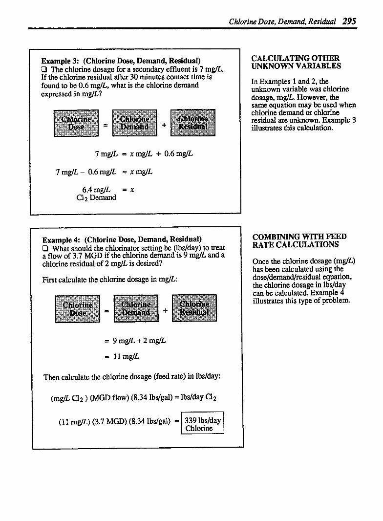
Chlorine Dose, Demand, Residual 295
Example 3: (Chlorine Dose, Demand, Residual) Q The chlorine dosage for a secondary effluent is 7 mglL. If the chlorine residual after 30 minutes contact time is found to be 0.6 mg/L, what is the chlorine demand expressed in mg/L?
6.4 mglL = X Cl2 Demand
Example 4: (Chlorine Dose, Demand, Residual) O What should the chlorinator setting be (lbs/day) to treat a flow of 3.7 MGD if the chlorine demand is 9 m& and a chlorine residual of 2 mglL is desired?
First calculate the chlorine dosage in mglL:
Then calculate the chlorine dosage (feed rate) in lbs/&y:
(mglL C12 ) (MGD flow) (8.34 lbs/gal) = lbs/&y Cl2
(11 mg/L) (3.7 MGD) (8.34 lbslgal) = 339 lbslday I Chlorine /
CALCULATING OTHER UNKNOWN VARIABLES
In Examples 1 and 2, the unknown variable was chlorine dosage, mglL. However, the same equation may be used when chlorine demand or chlorine residual are unknown. Example 3 illustrates this calculation.
COMBINING WITH FEED RATE CALCULATIONS
Once the chlorine dosage (mglL) has been calculated using the dose/demand/residual equation, the chlorine dosage in lbslday can bc calculated. Example 4 illustrates this type of problem.

296 Chapter 14. CHEMICAL DOSAGE
14.3 CHEMICAL FEED RATE--(Dosing Chemicals Less Than Full Strength)
HYPOCHLORITE COMPOUNDS
When chlorinating water or wastewater with chlorine gas, there is 100% available chlorine. Therefore, if the chlorine demand and residual require 50 lbslday chlorine, the chlorinator setting would be just that-50 lbsl24 hrs.
Many times, however, a chlorine compound called hypochlorite is used to chlorinate wastewater. Hypoc hlorite compounds contain chlorine and are similar to a strong bleach.
Because hypochlorites are not 100% pure chlorine more lbsfday must be fed into the system to obtain the same amount of chlorine for disinfection.
To calculate the lbslday hypo- chlorite required:
1. First calculate the lbslday chlorine required.
2. Then calculate the lbslday hypochlorite needed by dividing the lbslday chlorine by the percent available chlorine.
Hypochlorite - - lbslda~ Cl2 l bslday % Available Cl 2
100
Example l: (Chemical Feed Rate) P A total chlorine dosage of 12 mglL is uired to mat a particular water. If the flow is 1.2 MGD an 7 the hypo- chlorite has 65% available chlorine, how many lbslday of hypochlorite will be required?
First, calculate the lbslday chlorine required using the mg/L to lbslday equation:
(m@. C12 ) (MGD flow) (8.34 lbslgal) = lbslday Cl2
(12 mglL) (1.2 MGD) (8.34 lbslgal) = 1 120 lbslday I Then calculate the lbslday hypochlorite required. Since only 65% of the hypochlorite is chlorine, more than 120 lbsldav will be required:
Hyp~~hlorite - IbsIday C12 - l bslda y % Available C1 2
- 0.65 Avail. Cl2
- - 1 Hypochlorite 1851bs1day 1 Example 2: (Chemical Feed Rate) O A wastewater flow of 850,000 requires a chlorine dose of 25 mg/L. If hypochlorite ( % available chlorine) is to be used, how many lbslday of hypochlorite are required?
First, calculate the lbslday chlorine required:
(mglL C12 ) (MGD flow) (8.34 lbs/gal) = lbslday
(25 mglL) (0.85 MGD) (8.34 lbslgal) = I 17t:","h",y I Then calculate the lbslday hypochlorite:
Hypochlorite - lbslday Cl2 lbsIday - % Available C1 2
-
100 - - 177 lbs/day C1 2
0.65 Avail. C1 2
= ( 272 lbslday I Hypochlorite

Chemical Feed Rate 297
Example 3: (Chemical Feed Rate) Ll The desired dose of a polymer is 8 m& The polymer literature indicates that the polymer compound provided is 60% active polymer. If a flow of 4.4 MGD is to be treated, how many lbs/day of the polymer compound will be required?
First calculate the lbs/day polymer required:
(mglL Polymer) (MGD flow) (8.34 lbs/gal) = lbslday Polymer -
(8 mglL) (4.4 MGD) (8.34 lbslgal) = I 294 lbs/day I Polvmer
Then calculate the lbs/day polymer compound required:
Polymer Compound lbslda~ polymer l bs/day % Active Polvmer
Example 4: (Chemical Feed Rate) O A total of 695 lbs of 65% h ochlorite are used in a day. If the flow rate treated is 880,000 gpd, what is the chlorine dosage in mglL?
First calculate the 1bsJday chlorine dos age:
Hypochlorite , lbsIday cl2 lbslday % Available C1 2
100 695 lbs/day = lbs/day C1 2
H ypochlorite 0.65
Then calculate mglL Clz, using the mglL to lbs/&y equation and filling in the known information:*
(X mglL Cl2 ) (4.78 MGD) (8.34 lbslgal) = 452 lbslday Cl2
X = 452 lbs/day (4.78 MGD) (8.34 lbslgal)
OTHER CHEMICALS LESS THAN FULL STRENGTH
Other chemicals used in wastewater may be less than full strength, or less than 100% active. For example some polymers are less than 100% active. Be sure to check the chemical literature to determine whether or not it is 100% active. If a chemical is less than 100% "available chemical", calculate the lbslday dosing requirement using the same equation as a hypochlorite problem. Example 3 illustrates this calculation.
CALCULATING mglL CHLORINE GIVEN HYPOCHLOrnE
Occasionally you will know the lbs Jday hypoch1orite and will want to determine either the lbslday chlorine or the mglL chlorine. To calculate either of these unknown, begin with the hypochlorite equation and then, if needed, use the mglL to lbs/day equation. In effect, it is working the problem "backwards" from the problem shown in Example 2. Example 4 illustrates this type of calculation.
Refer to Chapter 2 in Basic Math Concepts for a review of solving for the unknown value.

298 Chapter 24 CHEMICAL DOSAGE
14.4 PERCENT STRENGTH OF SOLUTIONS
PERCENT STRENGTH USING DRY CHEMICALS
The strength of a solution is a measure of the amount of chemical (solute) dissolved in the solution. Since percent is calculated as "part over whole,"
percent strength is calculated as part chemical, in lbs, divided by the whole solution, in lbs:
% Strength = Chemical, lbs Solution, lbs
The denominator of the equation (lbs solution) includes both chemical (lbs) and water (lbs). Therefore the equation can be written in expanded form as:
% = Chemical, lbs
Strength Water + Chemical X loo
lbs lbs
As the two equations above illustrate, the chemical added must be expressed in pounds. If the chemical weight is expressed in ounces (as in Example 1) or grams (as in Example 2), it must f i t be converted to pounds (to correspond with the other units in the problem) before percent strength is calculated.
TWO PARTS OF A SOLUTION
@ SOLUTE Chemical to be added
dry liquid
@ SOLVENT
SOLUTION
Example 1: (Percent Strength) O If a total of 8 ounces of dry polymer are added to 10 gallons of water, what is the percent strength (by weight) of the polymer solution?
Before calculating percent strength, the ounces chemical must be converted to lbs chemical:*
8 ounces = 0.5lbschemical
16 ouncesJpound
Now calculate percent strength:
% Strength = Chemical, lbs X 100 Water, lbs + Chemical, lbs
- - 0.5 lbs Chemical X 100
(10 gal) (8.34 lbs/gal) + 0.5 lbs
- - 0.5 ibs Chemical 84 lbs Solution
* To review ounces to pounds conversions refer to Chapter 8 in Basic Math Concepts.

Percent Strength 299
Example 2: (Percent Strength) D If 100 grams of dry polymer are dissolved in 5 gallons of water, what percent strength is the solution? (1 gram = 0.0022 lbs)
F i t , convert grams chemical to pounds chemical. Since 1 gram equals 0.0022 lbs, 100 grams is 100 times 0.0022 lbs:
(100 grams) (0.0022 lbs/gram) = 0.22 lbs Chemical Chemical
Now calculate percent strength of the solution:
% Strength = lbs Chemical X 100
lbs Water + lbs Chemical
- - 0.22 lbs Chemical X 100
(5 gal) (8.34 lbs/gal) + 0.22 lbs
- - 0.22 lbs 41.92 lbs
Example 3: (Percent Strength) P How many pounds of ?P lymer must be added to 25 gallons of water to make a o polymer solution:
First, write the equation as usual and fill in the known infoxmation. Then solve for the unknown value.**
% Strength = lbs Chemical X 100
lbs Water + lbs Chemical
x lbs Chemical 1 = X 100
(25 gal) (8.34 lbslgal) + x lbs Chem.
/ 2.llbs ( = X Chernic a1
WHEN GRAMS CHEMICAL ARE USED
The chemical (solute) to be used in making a solution may be measund in grams rather than pounds or ounces. When this is the case, convert grams of chemical to pounds of chemical before calculating pexcent strength. The following relationship is used for the conversion:
SOLVING FOR OTHER UNKNOWN VARIABLES
In the percent strength equation there are three variables:
% Strength
lbs Chemical
lbs Water
In Examples 1 and 2, the unknown value was percent strength. However, the same equation can be used to determine either one of the other two variables. Example 3 illustrates this type of calculation.
Note that gallons water can also be the unknown variable in percent strength calculations. First set pounds water as the unknown variable in the equation. Then after the pounds water has been calculated convert pounds water to gallons water, using the 8.34 lbs/gd factor.*
* For a review of lbs to gallons conversions refer to Chapter 8 in Basic Moth Concepts. * * To review solving for the unknown value, refer to Chapter 2 in Basic Moth Concepts.

300 Chapter 14 CHEMICAL DOSAGE
PERCENT STRENGTH USING LIQUID CHEMICALS
When using a liquid chemical to make up a solution, such as liquid polymer, a different calculation is required.
The liquid chemical is shipped from the supplier at a certain percent strength-perhaps 10 or 12%. This chemical is then added to water to obtain a desired solution of lower percent polymer-such as 1 or 0.5%.
Percent strength calculations using liquid chemicals are very similar to sludge thickening calculations.* In sludge thickening problems, lbs solids are set equal to lbs solids. In these percent strength problems, lbs chemical are set equal to lbs chemical, as illustrated by the diagram to the right.
THE KEY TO THESE CALCULATIONS-POUNDS CHEMICAL REMAINS CONSTANT
(Liquid polymer is used to illustrate the concept.)
POLYMER SOLUTION
Simplified Equation:
I
(Liq. Poly.) (10.2) (% Strength) = (Poly. Soln) (8.34) (%Strength) gal lbs/gal of Liq. Poly. gal lbdgal of Poly. Soh.
loo loo
lbs Polymer - lbs Polymer in Liquid Polymer - in Polymer Solution
Expanded Equation:
(Liquid) (96 Strength) (Polymer) (%Strength) Polymer, of Liq- PO~Y . = Solution, of Poly. Soln.
lbs 100 lbs 100
Use mual density factor here. Use factor here. 1 Liquid polymer generally weighs Liquid polymer m& have a more than 8.34 lbslgal. Other density closer to or equal to 834 liquid chemicals may have the Ibs/gal since the heavy polymer - - .
same density ar wkr. has been diluted.
Example 4: (Percent Strength) P A 10% liquid polymer is to be used in making up a polymer solution. How many lbs of liquid polymer should be mixed with water to produce 150 lbs of a 0.8% polymer solution?
(Liquid Polymer) (% Strength) = (Pol . Soln.) (%Strength) lbs of Liq. Poly. 6s of Poly. Soh.
100 loo
(X lbs) ( 10 ) = (150 1bs) (0.8) - 100 loo
X = (150) (0.008)
0.1
* Refer to Chapter 15, Section 15.3.

Percent Strength 301
Example 5: (Percent Strength) 0 How many gallons of 8% liquid polymer should be mixed with water to produce 75 gallons of a 0.5% polymer solution? The density of the polymer liquid is 10.2 lbs/gal. Assume the density of the polymer solution is 8.34 lbsfgal.
Use the expanded form of the equation, filling in known idonnation:
(Liq. Po~Y.) (10.2) (% seen@) = (Poly. Soln) (8.34) (%Strength) gal lbs/gal of Liq. Poly. gal lbs/gal of Poly. Soln.
X ' 1 3.8 gallons I
Example 6: (Percent Strength) P A 10% liquid polymer will be used in makin up a P; solution. How many gallons of liquid polymer S odd be added to the water to make up 60 gallons of 0.4% polymer solution? The liquid polymer has a specific gravity of 1.1 Assume the polymer solution has a specific gravity of 1.0.
First, convert specific gravity information to density information. The density of the liquid polymer is (8.34 lbdgal) (1.1) = 9.2 lbs/gal. The density of the polymer solution is 8.34 lbs/gal, the same as water.
Poly.) (9.2) (% sangth) - (Poly. Soln) (8.34) (%Strength) gal lbslgal of Liq. Poly. gal lbdgal of Poly. Soln.
100 100
(X gal) (9.2) ( - 10 ) = (60 gal) (8.34) (0.4) - 100 100
X = (60) (8.34) (0.004) (9.2) (0.1)
DENSITY AND SPECIFIC GRAVITY CONSIDERATIONS
As shown in the second expanded equation on the opposite page, the density of the solution must be included. Density is the mass per unit volume.* In water and was tewater calculations, 8.34 lbs/gal is used as the density of water. However, the weight of a polymer solution can be as much as 10 or l l lbslgal. To obtain accurate results using the percent strength equation, it is important to use the appropriate density factor-ne for the solute (such as liquid polymer) and another for the solution. When the solution strength is very low, such as 0.5% or 0.196, the density of the solution is normally much closer to that of water-8.34 lbslgal.
Occasionally specific gravity data may be given for a liquid chemical rather than density information. In fact, density and specific gravity are closely related terms. Density is a measure of the mass per unit volume, and is measured in such terms as lbslgal. Specific gravity is a comparison of the density of a substance to a standard density. (For liquids, the standard is water. All other densities are compared to the density of water.) So, a specific gravity of 1.0 means the liquid has the same density as water (8.34 ibs/gal). A specific gravity of 0.5 means the liquid has a density half that of water, or 4.17 lbslgal. A specific gravity of 1.5 means the liquid has a density 1.5 times that of water, or 12.51 lbslgal. Example 6 illustrates a calculation including specific gravity data.
* Refer to Chapter 7, Section 7.1, "Density and Specific Gravity".

302 Chapter 14. CHEMICAL DOSAGE p- P p
14.5 MIXING SOLUTIONS OF DIFFERENT STRENGTH
There are two types of solution mixture calculations. In one type of calculation, two solutions of different strengths are mixed with no particular target solution strength. The calculation involves deter- mining the percent saength of the solution mixture.
The second type of solution mixture calculation includes a desired or target strength. This type of problem is described in the next section.
WHEN DDTERENT PERCENT STRENGTH SOLUTIONS ARE MIXED
10% Strength 1 % Strength Solution Mixture Solution Solution (% Strength somewhere
between 10% and 1% depending on the quantity
Simplified Equation: contributed by each.)
Strength = Chemical in Mixture, lbs I of Mixture Solution Mixture, Ibs
Expanded Equations:
lbs Chem. from lbs Chem. from % Strength Solution 1 + Solution 2 of Mixture - lbs Solution 1 + lbs Solution 2 X 100
(Sol'n 1) (% Smngth) (Sol'n 2) (% Strength) lbs ofSol'n1 + lbs ofSol'n2
% Strength = 100 of Mixture lbs Solution 1 + lbs Solution 2
loo X loo
Example 1: (Solution Mixtures) P If 20 lbs of a 10% strength solution are mixed with 50 lbs of 1% strength solution, what is the percent strength of the solution mixture?
(Sol'n 1) (% Strength) (Sol'n 2) (% Strength) lbs of S o h 1 + lbs of S o h 2
% Strength = 100 of Mixture
loo X loo lbs Solution 1 + lbs Solution 2
2 1bs + 0.5 1bs 100 70 lbs

Solution Mixtures 303
Example 2: (Solution Mixtures) P If 5 gallons of an 8% sangth solution are mixed with 40 gallons of a 0.5% strength solution, what is the percent strength of the solution mixture? (Assume the 8% solution weighs 9.5 lbslgal and the 0.5% solution weighs 8.34 lbs/gal.)
(Sol'n 1) (96 San@) (Soh 2) (% Strength) lbs ofSol'n1 + lbs ofSo11n2
% Smngth 100 of Mixture lbs Solution 1 + lbs Solution 2
loo X loo
- - (5 gal) (9.5 lbslgal) (0.08) + (40 gal) (8.34 lbslgal) (0.005) (5 gal) (9.5 lbslgal) + (40 gal) (8.34 lbslgal)
- - 3.8 lbs Chem. + 1.7 lbs Chem. 47.5 lbs Soln 1 + 333.6 lbs Soln 2
- - 5.51bsChemical xlOO 381 .l lbs Solution
= 11.4% Strength I
Example 3: (Solution Mixtures) D If 15 gallons of a 10% strength solution are added to 50 gallons of 0.8% strength solution, what is the percent strength of the solution mixture? (Assume the 10% strength solution weighs 10.2 lbslgal and the 0.8% strength solution weighs 8.8 lbslgal.)
(Sol'n 1) (96 Strength) (Soh 2) (% Strength) lbs of S o h 1 + lbs of Sol'n 2
% Strength = loo of Mixture lbs Solution 1 + lbs Solution 2
loo X loo
- - (15 gal) (10.2 lbdgal) (0.1) + (50 gal) (8.8 1bslp;al) (0.008) 100 (15 gal) (10.2 lbdgal) + (SO gal) (8.8 lbslgal)
- - 15.3 lbs Chem. + 3.5 lbs Chem. 100 153 lbs Soln 1 + 440 lbs Soln 2
- - 18.8lbsChemical 593 lbs Solution
= 1 3.2% Strength I
USE DIFFERENT DENSITY FACTORS WHEN APPROPRIATE
Percent strength should be expressed in terms of pounds chemical per pounds solution. Therefare, when solutions are expressed in terms of gallons, the gallons should be expressed as pounds befon continuing with the percent strength calculation.
It is important to know what density factor should be used to COnVeR from gallons to pounds. If the solution has a density the same as water. 8.34 lbs/gal is uscd If, however, the solution has a higher density, such as some polymer solutions, then the higher density factor should be used. When the density is unknown, it is sometimes possible to weigh the chemical solution to determine the density.

304 Chapter 14 CHEMICAL DOSAGE
SOLUTION MIXTURES TARGET PERCENT STRENGTH
In the previous section we examined the first type of solu- tion mixture calculation-a calculation where there is no target percent strength. In this type calculation, two solutions are mixed and the percent strength of the mixture is determined.
In the second type of solution mixture calculation, two dif- ferent percent strength solutions are mixed in order to obtain a desired quantity of solution and a target percent strength. These problems may be solved using the same equation shown in Examples 1-3. An illustration of this approach is given in Example 4.
Another and perhaps preferred approach in solving these pro- blems is by using the dilution rectangle. Although the fmt use of the dilution rectangle can be confusing, the effort to master its use is rewarded- solution mixture problems are quickly calculated. Example 5 uses the dilution rectangle to solve the problem stated in Example 4. Compare the two methods of calculating this type of mixture problem.
Example 4: (Dilution Rectangle) Q What weights of a 2% solution and a 7% solution must be mixed to make 850 lbs of a 4% solution? Use the same equation as shown for Examples 1-3 and fill in given information.* (Note that the lbs of Solution 1 is unknown, X. If lbs of Solution 1 is X, then the lbs of Solution 2 must be the balance of the 850 lbs, or 850-X.)
(Soh 1) (% Strength) (Soh 2) (% Strength) lbs of S o h 1 + lbs of Sol'n 2
% Strength - 100 of Mixture lbs Solution 1 + lbs Solution 2
loo X loo
(X lbs) (0.02) + (850 - X lbs) (0.07)x 4 =
850 lbs
Then 850 - 5 10 $ 340 1bs of 7% Solution l
0.05~ = 25.5
THE DILUTION RECTANGLE
X =
Higher % Solution
5 10 1bs of 2% Solution
Parts Higher % Solution
Lower % Parts Lower % Solution Solution
Steps in Using the Dilution Rectangle: 1. Place the % Strength numbers in positions A, B, and C.
2. Calculate parts higher % solution and parts lower % solution, subtracting as indicated.
3. Multiply fractional parts of each solution by the total lbs of solution desired.
* Refer to Chapter 2 in Bmic Math Concepts for a review of solving for the unknown value.

Dilution Rectangle 305
Example 5: (Dilution Rectangle) P What weights of a 2% solution and a 7% solution must be mixed to make 850 lbs of a 4% solution?
Use the Dilution Rectangle to solve this problem. First determine the parts required of each solution:
7 2 Parts of \ 7%soln
5 Parts Total
Thus, 2 parts of the total 5 parts (215) come from the 7% solution, and the other thnx parts (3/5) come from the 2% solution. Now calculate the lbs of 2% and 7% solution, using these fractions:
of 2 (850 lbs) = 7%Soln: 5
Amt. of 2 (850 lbs) = 2% Soln: c
Example 6: (Dilution Rectangle) O How many lbs of a 10% polymer solution and water should be mixed together to form 425 lbs of a 1% polymer solution?
First calculate the parts of each solution required:
1°\, f 1 Parts of 10% Soln
Parts of Water
10 Parts Total
Then calculate the actual lbs of each solution:
(1) Amto of - (425 lbs) = 10% Soln: 10
Amt* of (425 lbs) = Water: 10 Water
MIXING A SOLUTION AND WATER
In solution mixing Examples 1-5, two solutions of different strengths are blended. The solution mixing equation and dilution rectangle can also be used when only one solution and water are blended. (Water is considered a 096 strength solution.) Example 6 illustrates such a calculation using the dilution rectangle.
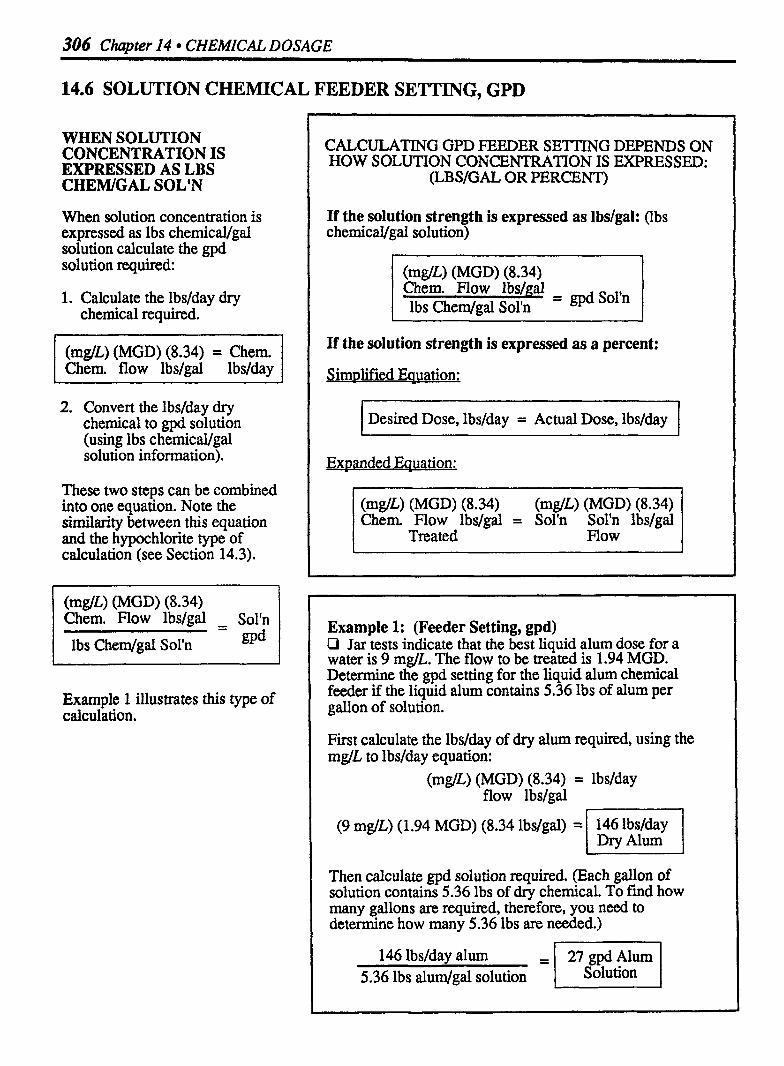
306 Chapter 14 CHEMICAL DOSAGE
14.6 SOLUTION CHEMICAL FEEDER SETTING, GPD
WHEN SOLUTION CONCENTRATION IS EXPRESSED AS LBS CHEWGAL SOL'N
When solution concentration is expressed as lbs chemicdgal solution calculate the gpd solution required:
1. Calculate the lbs/day dry chemical required.
(mglL) (MGD) (8.34) = Chem. Chem. flow lbs/gal lbs/day
2. Convert the lbs/day dry chemical to gpd solution (using ibs chernicaVga1 solution information).
These two steps can be combined into one equation. Note the similarity between this equation and the hypochlorite type of calculation (see Section 14.3).
(mglL) (MGD) (8.34) Chem. Flow lbslgal - Sol'n - lbs Chem/gal Sol'n g ~ d
Example 1 illustrates this type of calculation.
CALCULATING GPD FEEDER SETTING DEPENDS ON HOW SOLUTION CONCENTRATION IS EXPRESSED:
(LBS/GAL OR PERCENT)
If the solution strength is expressed as Ibsfgal: (lbs chemical/gal solution)
low ibs/gd lbs Chem/gal Sol'n = gpd Sol'n
If the solution strength is expressed as a percent:
simplified Eauation:
I Desired Dose, lbs/day = Actual Dose, lbs/dayI
Expanded Equation:
(mg/L) (MGD) (8.34) (rnglL) (MGD) (8.34) Chem. Flow lbs/gal = Sol'n Sol'n lbs/gal
Treated Flow
Example 1: (Feeder Setting, gpd) Cl Jar tests indicate that the best liquid alum dose for a water is 9 mglL. The flow to be treated is 1.94 MGD. Determine the gpd setting for the liquid alum chemical feeder if the liquid alum contains 5.36 lbs of alum per gallon of solution.
First calculate the lbslday of dry alum required, using the mgl . to lbslday equation:
(mg/L) (MGD) (8.34) = lbs/day flow lbs/gal
(9 mg/L) (1.94 MGD) (8.34 lbs/gal) = 146 lbdday ( Dry Alum 1 Then calculate gpd solution required. (Each gallon of solution contains 5.36 lbs of dry chemical. To find how many gallons m required, therefore, you need to determine how many 5.36 lbs are needed.)
146 lbs/day alum 5.36 lbs dudgal solution = / 27 Solution I
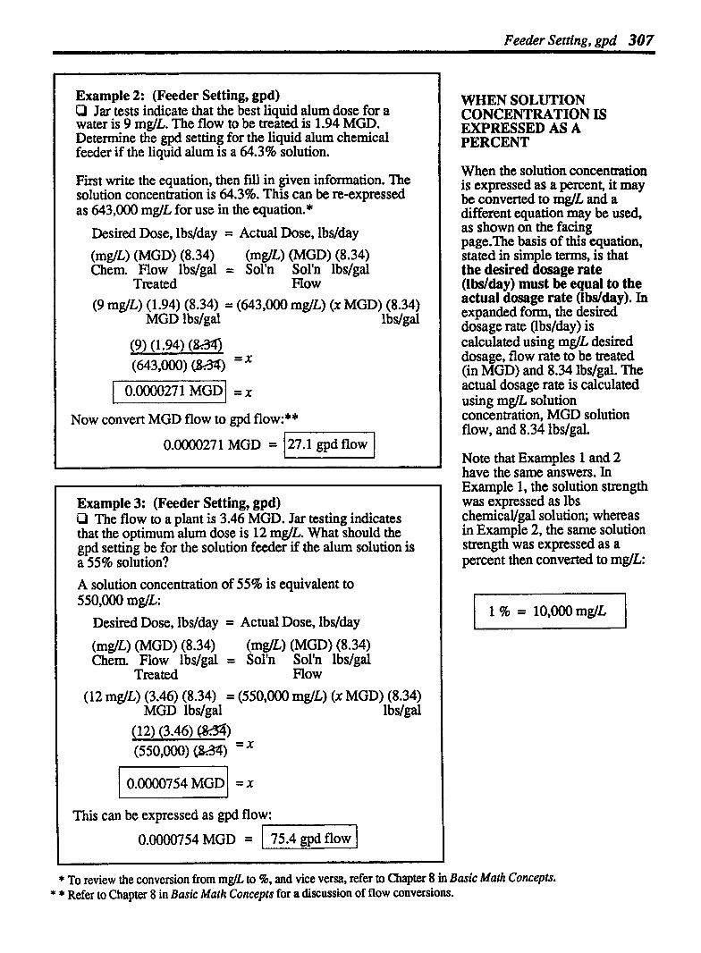
Feeder Setting, gpd 307
Example 2: (Feeder Setting, gpd) P Jar tests indicate that the best liquid alum dose for a water is 9 mglL. The flow to be treated is 1.94 MGD. Determine the gpd setting for the liquid alum chemical feeder if the liquid alum is a 64.3% solution.
F i t write the equation, then fill in given information. The solution concentration is 64.3%. This can be re-expressed as 643,000 mg/L for use in the equation.*
Desired Dose, lbs/day = Actual Dose, lbslday
(mg/L) (MGD) (8.34) (mglL) (MGD) (8.34) Chem. Flow lbs/gal = Sol'n S o h lbslgal
Treated How
(9 m@L) ( 1.94) (8.34) = (643,000 mglL) (X MGD) (8.34) MGD lbslgal lbslgal
Now convert MGD flow to gpd flow:**
O.OO27 1 MGD = 127.1 gpd flow I
Example 3: (Feeder Setting, gpd) P The flow to a plant is 3.46 MGD. Jar testing indicates that the optimum alum dose is 12 mg/L. What should the gpd setting be for the solution feeder if the alum solution is a 55% solution?
A solution concentration of 55% is equivalent to 550,000 mglL:
Desired Dose, lbslday = Actual Dose, lbslday
(mglL) (MGD) (8.34) (mglL) (MGD) (8.34) Chem. Flow lbs/gal = Sol'n S o h lbslgal
Treated How
(12 mdL) (3.46) (8.34) = (550,000 mglL) (X MGD) (8.34) MGD lbslgal l bslgal
This can be expressed as gpd flow:
0.0000754 MGD = 1 75.4 gpd flow I
WHEN SOLUTION CONCENTRATION IS EXPRESSED AS A PERCENT
When the solution concentration is expressed as a percent, it may be converted to mglL and a different equation may be used, as shown on the facing page.The basis of this equation, stated in simple terms, is that the desired dosage rate (lbdday) must be equal to the actual dosage rate (lbdday). I . expanded form, the desired dosage rate (lbslday) is calculated using mglL desired dosage, flow rate to be treated (in MGD) and 8.34 lbs/gal. The actual dosage rate is calculated using mglL solution concentration, MGD solution flow, and 8.34 lbslgal.
Note that Examples 1 and 2 have the same answers. In Example l, the solution strength was expressed as lbs chemical/gal solution; whereas in Example 2, the same solution strength was expressed as a percent then converted to mglL:
* To review the conversion from mglL to %, and vice versa, refer to Chapter 8 in Basic Math Concepts. * * Refer to Chapter 8 in Basic Math Concepts for a discussion of flow conversions.
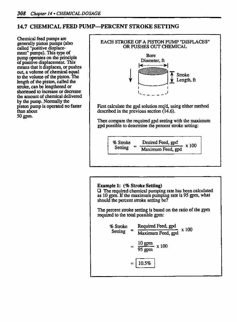
308 Chapter I4 CHEMICAL DOSAGE
14.7 CHEMICAL FEED PUMP-PERCENT STROKE SETTING
Chemical feed pumps are generally piston pumps (also called "positive displace- ment" pumps). This type of pump operates on the principle of positive displacement. This means that it displaces, or pushes out, a volume of chemical equal to the volume of the piston. The length of the piston, called the stroke, can be lengthened or shortened to increase or decrease the amount of chemical delivered by the pump. Nomally the piston pump is operated no faster than about 50 gpm.
EACH STROKE OF A PISTON PUMP "DISPLACES" OR PUSHES OUT CHEMICAL
Bore Diameter, ft
I r l
First calculate the gpd solution req'd, using either method described in the previous section (14.6).
Then compare the required gpd setting with the maximum gpd possible to determine the percent stroke setting:
% Stroke Desired Feed, gpd Setting = Maximum Feed, gpd
Example 1: (% Stroke Setting) Q The required chemical pumping rate has been calculated as 10 gpm. If the maximum pumpmg rate is 95 gpm, what should the percent stroke setting be?
The percent stroke setting is based on the ratio of the gpm required to the total possible gpm:
% Stmke Required Feed, gpd Setting = Maximum Feed, gpd
X 100
- - logpm X 1 0 0 95 gprn

% Stroke Setting 309
Example 2: (9% Stroke Setting) 0 The required chemical pumping rate has been calculated as 15 gpm. If the maximum pumping rate is 82 gpm, what should the percent stroke setting be?
% Stroke Required Feed, gpd Setting = Maximum Feed, gpd
- - = x loo 82 gpm
Example 3: (% Stroke Setting) Q The required chemical pumping rate has been determined to be 75 gpm. If the maximum pumping rate is 85 gpm, what should the percent stroke setting be?
% Stroke Required Feed, gpd Setting = Maximum Feed, gpd
- '5 X 100 85 gpm

310 Chapter 14 CHEMICAL DOSAGE
14.8 SOLUTION CHEMICAL FEEDER SETTING, d m i n
Some solution chemical feeders dispense chemical as milliliters per minute (mL/min). To calculate the d m i n solution required, first calculate the gpd feed rate, as described in Section 14.6. Then convert gpd flow rate to Wmin flow rate. The process, as shown in the equation to the right, involves the following conversions: * *
FIRST DETERMINE GPD FLOW THEN CALCULATE MIJMIN FLOW
Calculate gpd solution flow required:
Sim~Efied Equation:
Desired Dose, lbslday = Actual Dose, lbslday
Ex~anded Eauation:
(mg/L) (MGD) (8.34) = (mglL) (MGD) (8.34) Dose Flow lbslgal Sol'n Sol'n lbslgal
Treated Flow
Convert mUrnin solution flow required:*
(gal) (1 day) (3785 -
Or, simplified as:
Example 1: (Feeder Setting, mLJmin) P The desired solution feed rate was calculated to be 8 gpd. What is this feed rate expressed as mUmin?
Since the gpd flow has already been determined, the mL/min flow rate can be calculated directly:
* This equation is written in a form so that dimensional analysis may be used to check the units of the answer. Refer to Chapter 15 in Basic Math Concepts.
* * Refer to Chapter 8 in Basic Math Concepts for flow rate and metric conversions.

Feeder Setting, d m i n 311
Example 2: (Feeder Setting, mllmin) O The desired solution feed rate has been calculated to be 20 gpd. What is this feed rate expressed as mUmin?
Since the gpd solution feed rate has been determined, the ml/min may be calculated directly:
Example 3: (Feeder Setting, mllmin) Q The optimum polymer dose has been determined to be 12 m&. The flow to be treated is 980,000 gpd. If the solution to be used contains 60% active polymer, what should the solution chemical feeder setting be, in mZ,/min?
First calculate the -g@ feed rate required:
(mglL) (MGD) (8.34) = (mglL) (MGD) (8.34) Chem flow lbs/gal S o h Sol'n Ibs/gal Dose treated flow
(1 2 m@) (0.98 MGD) (8.34) = (600,000) (X MGD) (8.34) Pol y m. lbslgal mg/L lbslgal
(12) (0.98) M ( 6 0 0 , ~ ) M
= X MGD
0.0000196 MGD = x
Then convert gpd flow rate to m4min flow rate:
(gpd) (3785 mWgal) 1440 minjday = ml/Inin

312 Chapter 14 CHEMICAL DOSAGE
14.9 DRY CHEMICAL FEED CALIBRATION
Occasionally you will want to compare the actual chemical feed rate with the feed rate indicated by the instrumen- tation. This is called a calibra- tion calculation.
To calculate the actual chemical feed rate for a dry chemical feeder, place a bucket under the feeder, weigh the bucket when empty, then weigh the bucket again after a specified length of time, such as 30 minutes.
The actual chemical feed rate can then be determined as:
Chem. Faxi = Chem. Applied, lbs Rate, Length of Applic, min
lbslmin
The chemical feed rate can be converted to lbslday, if desired:
Example 1: (Dry Chemical Feed Calibration) Ll Calculate the actual chemical feed rate, lbslday, if a bucket is placed under a chemical feeder and a total of 1.5 lbs is collected during a 30-minute period.
First calculate the lbslmin feed rate:
Chem Feed - Chem. Applied, lbs Rate, lbslmin - Length of Application, min
- -- 1.5 lbs 30 min
= 1 0.05 lbs/min I Feed Rate
Then calculate the lbs/day f e d rate:
Chem. Feed = (0.05 lbslmin) (1440 midday) Rate, lbslday
Example 2: (Dry Chemical Feed Calibration) Q Calculate the actual chemical feed rate, lbslday , if a bucket is placed under a chemical feeder and a total of 1.3 lbs is collected during a 20-minute period.
First calculate the lbslmin feed rate:
Chem. Feed - Chem. Applied, lbs Rate, lbdfin Length of Application, min
- - 1.3 lbs 20 min
- 1 0.065 lbs/min ( Feed Rate
Then calculate the lbslday feed rate:
Chem Feed = (0.065 lbs/min) (1440 midday) Rate, lbs/day
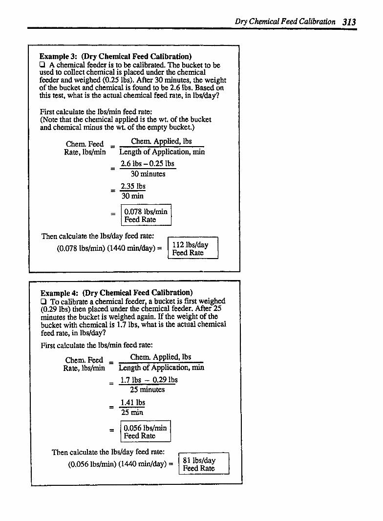
Dry Chemical Feed Calibration 313
Example 3: (Dry Chemical Feed Calibration) Q A chemical feeder is to be calibrated. The bucket to be used to collect chemical is placed under the chemical feeder and weighed (0.25 lbs). After 30 minutes, the weight of the bucket and chemical is found to be 2.6 lbs. Based on this test, what is the actual chemical feed rate, in lbs/day?
First calculate the lbs/rnin feed rate: (Note that the chemical applied is the wt. of the bucket and chemical minus the wt. of the empty bucket.)
Chem. Feed = Chem. Applied, lbs Rate, lbs/min Length of Application, min
30 minutes
- - 2.35 lbs 30 min
= 1 0.078 lbs/min 1 Feed Rate
Then calculate the lbs/day feed rate: ,-, (0.078 lbs/min) (1440 midday) = Feed Rate I 112 lbsfday l
Example 4: (Dry Chemical Feed Calibration) O To calibrate a chemical feeder, a bucket is first weighed (0.29 lbs) then placed under the chemical feeder. After 25 minutes the bucket is weighed again. If the weight of the bucket with chemical is 1.7 lbs, what is the actual chemical feed rate, in lbslday?
First calculate the lbs/min feed rate:
Chem. Feed , Chem. Applied, lbs Rate, lbs/min Length of Application, min
- - 1.7 1bs - 0.29 1bs 25 minutes
= / 0.056 lbs/min I Feed Rate
Then calculate the ibs/day feed rate:
(0.056 lbslmin) (1440 midday) = I Feed Rate *lLbsfday I

314 Chapter I4 CHEMICAL DOSAGE
14.10 SOLUTION FEED CALIBRATION (Given ~ d l m i n Flow)
The calibration calculation for a solution feeder is slightly more difficult than that for a dry chemical feeder.
As with other calibration calculations, the actual chemical feed rate is determined and then compared with the f e d rate indicated by the instrumenta- tion.
To calculate the actual chemical feed rate for a solution feeder, first express the solution feed rate in terms of MGD. (The equation for converting fiom N m i n to gpd is given to the right.) Once the MGD solution flow rate has been calculated, use the mglL, equation to determine chemical dosage in lbslday .
SOLUTION FEED CALIBRATION
First convert mLlmin flow rate to gpd flow rate
Then calculate chemical dosage, Wday
(m@, Chem.) (MGD Flow) (8.34 lbslday) = Chem., l bs/day
Example l: (Solution Chemical Feed Calibration) 01 A calibration test is conducted for a solution chemical feeder. During 5 minutes, a total of 750 m[, is delivered by the solution fteder. The polymer solution is a 1.2% solution. What is the lbslday feed rate? (Assume the polymer solution weighs 8.34 lbslgal.)
Normally the mg/L to lbslday equation* is used to determine the lbs/day fced rate. And in making these calculations, the flow rate must be expressed as MGD. Therefore, the m n flow rate must first be converted to gpd and then MGD. The a m i n flow rae is calculated as:
Then convert m4min flow rate to gpd flow rate:
3785 Wgal I flow rate I And calculate lbslday feed rate: ** (mg/L Qlem.) (MGD Flow) (8.34 lbslday) = lbslday Chem.
(12,000 mglL ) (0.000057 MGD) (8.34 lbs/day) = 5.7 lbs/day l Polymer l * A detailed discussion of the mg/L to Ibslday calculation is given in Chapter 3.
* * A solution of 1.2% strength is equivalent to a solution of 12,000 mg/L concentration. Refer to Chapter 8 in Baric Math Concepts for a discussion of mglL to % conversions.
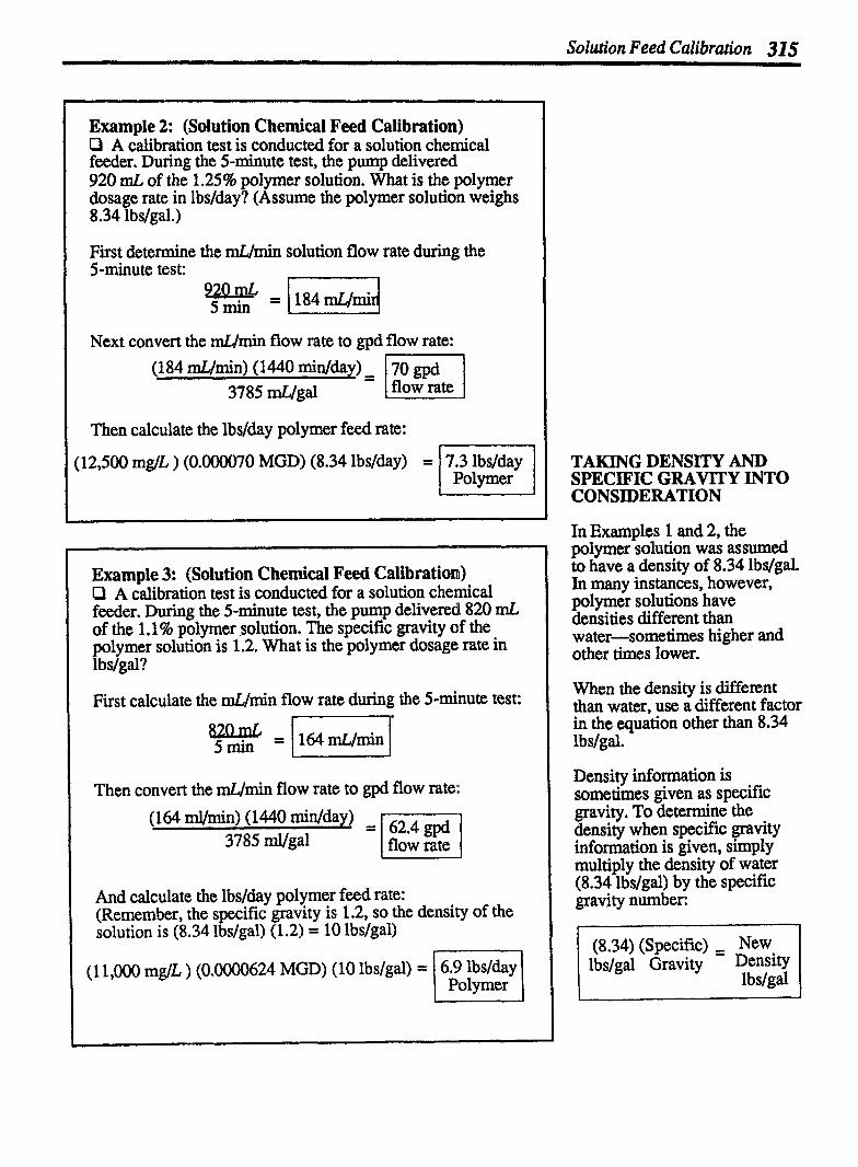
Solution Feed Calibration 31 5
Example 2: (Solution Chemical Feed Calibration) Cl A calibration test is conducted for a solution chemical feeder. During the 5-minute test, the pump delivered 920 mL of the 1.25% polymer solution. What is the polymer dosage rate in lbslday? (Assume the polymer solution weighs 8.34 lbslgal.)
First determine the mL/min solution flow rate during the 5-minute test: . 4
Next convert the mL/min flow rate to gpd flow rate: (184 mU/min) (1440 midday)
= 3785 &gal flow rate
Then calculate the lbslday polymer feed rate: I 1
(12,500 mg/L ) (0.000070 MGD) (8.34 lbs/day) 1 Polymer = 7*3 lbsIday I
Example 3: (Solution C hernial Feed Calibration) C l A calibration test is conducted for a solution chemical feeder. During the 5-minute test, the pump delivered 820 mL. of the 1.1 % polymer solution. The specific gravity of the polymer solution is 1.2. What is the polymer dosage rate in l bs/gal?
First calculate the mllmin flow rate during the 5-minute test:
= 1164mrJmin 1 5 min
Then convert the d m i n flow rate to gpd flow rate:
And calculate the lbslday polymer feed rate: (Remember, the specific gravity is 1.2, so the density of the solution is (8.34 lbslgal) (1.2) = 10 lbslgal)
(1 1,000 mg/L ) (0.0000624 MGD) (10 lbs/gal) = 6.9 lbs/day \ polymer l
TAKING DENSITY AND SPECIFIC GRAVITY INTO CONSIDERATION
In Examples 1 and 2, the polymer solution was assumed to have a density of 8.34 ibs/gal h many instances, however, polymer solutions have densities different than water-sometimes higher and other times lower.
When the density is different than water. use a different factor - - - . -
in the equation other than 8.34 lbslgal.
Density information is sometimes given as specific gravity. To determine the density when specific gravity information is given, simply multiply the density of water (8.34 lbs/gal) by the specific gravity number:
(8.34) (Specific) = New lbs/gal Gravity Density
lbslgal

316 Chapter 14 CHEMICAL DOSAGE
14.11 SOLUTION CHEMICAL FEED CALIBRATION (Given Drop in Solution Tank Level)
Actual pumping rates can be determined by calculating the volume pumped during a specified time frame. For example, if 50 gallons are pumped during a 10-minute test, the average pumping rate during the test is 5 gpm.
The gallons pumped can be determined by measuring the drop in water level during the timed test.
VOLUME PUMPED IS INDICATED BY DROP IN TANK LEVEL
Diameter, ft W D + l
J. Drop in Solution Level, ft
Simplified Equation:
Flow , - Volume Pumped, gal gpm Duration of Test, min
Expanded Equation:
~l~~ Rate - (0.785) ( D ~ ) m o p in Level, ft) (7.48 gucu ft) - Duration of Test, min
Example 1: (Solution Feeder Calibration) Q A pumping rate calibration test is conducted for a 5-minute period. The liquid level in the 3-ft diameter solution tank is measured before and after the test. If the level drops 1.2 ft during the 5-min test, what is the pumping rate in gpm?
J. 1.2 ft Drop
Flow Rate , - (0.785) (D 2, (Drop, ft) (7.48 gaVcu ft) @m Duration of Test, min
- (0.785) (3 ft) (3 ft) (1.2 ft) (7.48 gaVcu ft)
Pumping Rate =l 13gpm l

Solution Feeder Calibration 31 7
Example 2: (Solution Feeder Calibration) O A pumping rate calibration test is conducted for a 4-minute period. The liquid level in the 4-ft diameter tank is measured before and after the pumping test. If the level drop is 10 inches during the test, what is the pumping rate in gpm?
Flow Rate , - (0.785) (02) (Drop, ft) (7.48, gdcu ft) Duration of Test, min
- - (0.785) (4 ft) (4 ft) (0.83 ft) (7.48 gaVcu fi)
Example 3: (Solution Feeder Calibration) P A pump test indicates that a pump delivers 45 Frn during a 5-minute pumping test. The diameter oft e solution tank is 3 feet. What was the ft drop in solution level during the pumping test?
J. xft
Flow Rate , c. (0.785) (D*) (Drop, ft) (7.48 gal/cu ft) Duration of Test, min
45 = (0.785) (3 ft) (3 ft) (xft) (7.48 gdcu ft)
I .
Now solve for the unknown value*:
(45) (5) (0.785) (3) (3) (7.48)
= X ft Drop
CALCULATING OTHER UNKNOWN VARIABLES
In Examples 1 and 2, the unknown variable was gpm pumping rate. The same equation can be used to solve for any one of the other variables: gpm pumping rate, tank diameter, level drop, or duration of test. In Example 3, the level drop is the unknown variable.
* Refer to Chapter 2 in Basic Math Concepts for a review of solving for the unknown value.

318 Chapter 14 CHEMICAL DOSAGE
14.12 AVERAGE USE CALCULATIONS
The lbslday or gpd chemical use should be recorded each day. From this data, you can calculate the average daily use of the chemical or solution.
From this information you can forecast expected chemical use, compare it with chemical in inventory, and determine when additional chemical supplies will be required.
AVERAGE CHEMICAL USE
First determine the average chemical use:
Average Use Total Chem. Used, lbs I lbslday Number of Days
Then calculate day's supply in inventory:*
Day's Supply - Total Chem. in Inventory, lbs - in Inventory Average Use, lbs/day
Day's Supply = Total Chem in Inventory, gal in Inventory Average Use, gpd
Example 1: (Average Use) Q The chemical used for each day during a week is given below. Based on this data, what was the average lbslday chemical use during the week?
Monday-90 lbs/day Tuesday-96 lbslday Wednesday-92 lbslday Thursday-89 lbslday
Friday-98 lbslday S aturday-9 l lbslday Sunday-87 lbslday
Average Use Total Chem. Used, Ibs l bslday
- Number of Days
- - 643 lbs 7 days
= 91.9 lbslday I ~ v e r . Use I
* Note how similar these equations are to detention time equations.
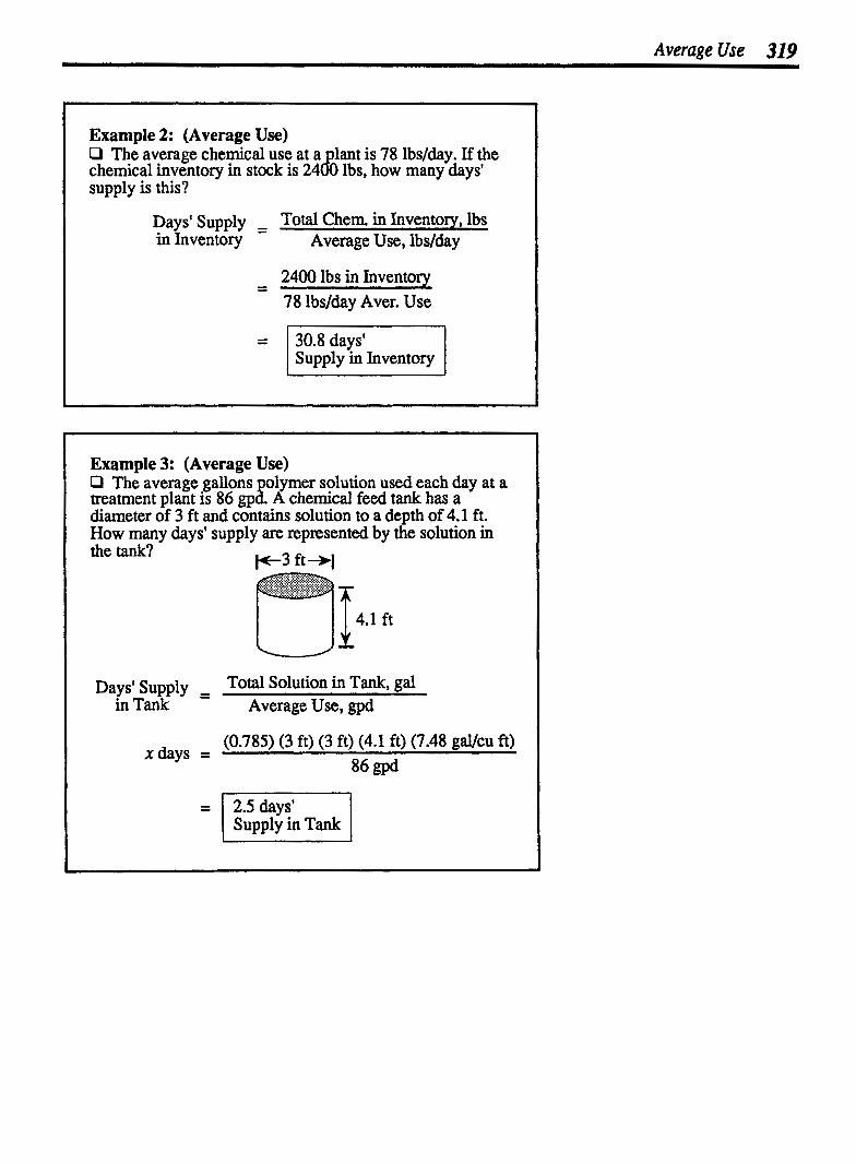
Average Use 319
Example 2: (Average Use) O The average chemical use at a lant is 78 lbs/day. If the chemical inventory in stock is 24 lbs, how many days' supply is this?
0 Days' Supply - Total Chem. in InventoryJbs in Inventory Average Use, lbslday
2400 lbs in Inventorv - 781bs/day AV&=. Use
Example 3: (Average Use) D The average gallons olymer solution used each day at a treatment plant is 86 gp8 A chemical feed tank has a diameter of 3 ft and contains solution to a depth of 4.1 ft. How many days' supply are represented by the solution in
=
the tank?
30.8 days' Supply in Inventory
Days1 supply - Total Solution in Tank, gal - in Tank Average Use, gpd
xdays = (0.785) (3 ft) (3 ft) (4.1 ft) (7.48 gaVcu ft)
86 gpd

1 5 Sludge Production and Thickening
1. Primary and Secondary Clarifier Solids Production
For R i m a ~ Clarifier;
For Secondarv C1
A Y-value, bacteria growth rate, is used to deternine SS produced in a secondary clarifier. The Y-value is the Zbslday of SS generated as a result of each lb of BOD conrwned, or removed, during treatment. Typical Y-values are established for each plant based on the average ratio of lbs SSilb BOD removed by the seconhy system . The equation below asswnes a Y-value, or growth rate, of 0.45 ibs SS producecillb BOD removed. The Y-value is established for each plant.
First calculate lbs/day BOD removed:
BOD Removed (mp/L)
(mg/L) (MGD) (8.34) = BOD BOD flow lbs/gal Removed
Removed lbdday
Then use the Y-value as a ratio to determine lbs/day SS produced:
0.45 lbs SS - x lbs SS 1 lb BOD Removed lbs/day BOD Removed
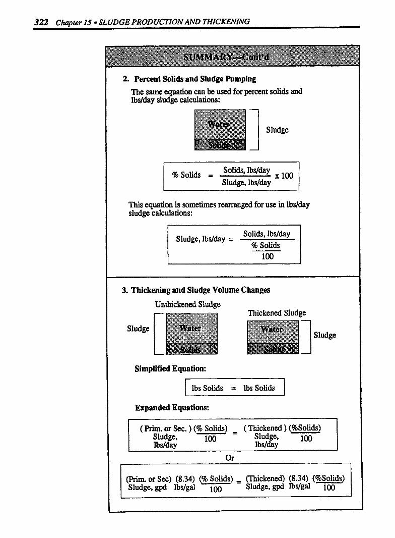
322 Clraoter IS SLUDGE PRODUCTION AND THICKENING
2. Percent Solids and Sludge Pumping The same equation can be used for percent solids and lbs/day sludge calculations:
% Solids = Solids, lbslday Sludge, lbs/day
This equation is sometimes rearranged for use in lbslday sludge calculations:
l Sludge, lbs/day = Solids, lbslday 1
% Solids
1 3. Thickening and Sludge Volume Changes
I Unthickened Sludge Thickened Sludge
Simplified Equation:
lbs Solids = Ibs Solids
I Expanded Equations:
( Prim. or Sec. ) (% Solids) - ( Thickened ) (%Solids) Sludge, 100 - Sludge, lbslday lbslday
100
l l (Prim. or Sec) (8.34) (46 Solids) = (Thickened) (8.34) (%Solids) Sludge, gpd lbslgal 100 Sludge, gpd lbsfgal 100 I
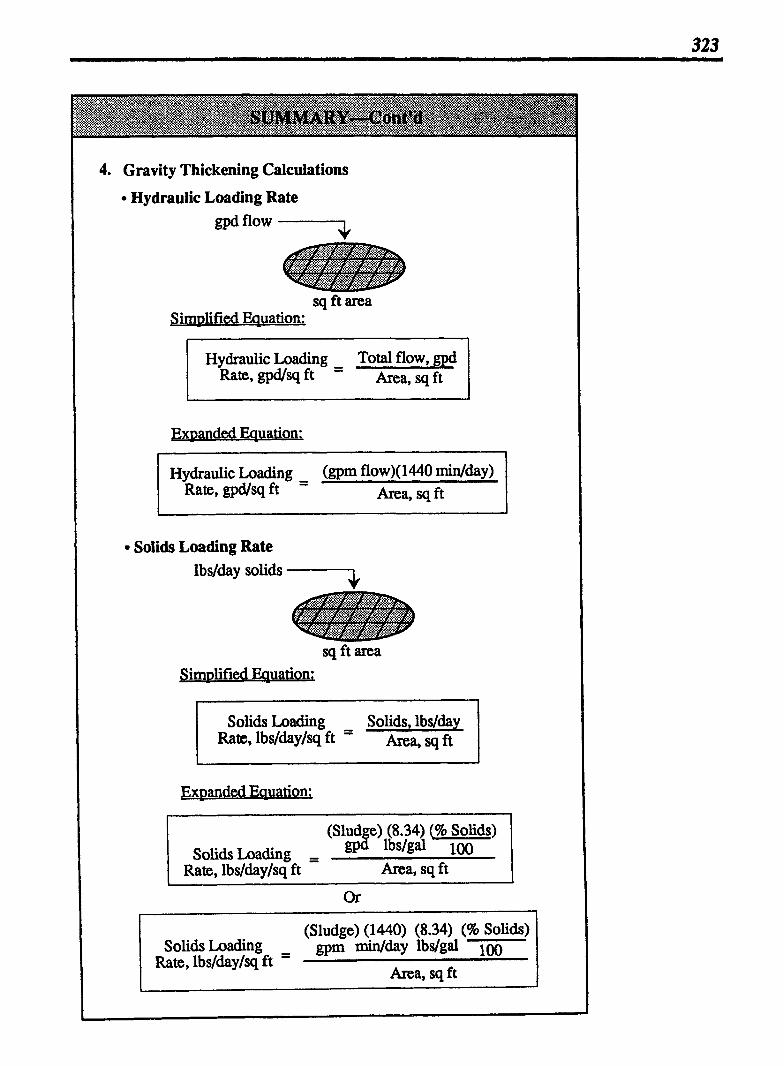
4. Gravity Thickening Calculations
Hydraulic Loading Rate
sq ft area Simplified Equation;
Hydraulic Loading - Total flow, gpd Rate, gpd/sq ft Area, sq ft
Ex~anded Eauation: I I
Solids Loading Rate lbs/day solids 7
sim~lified Equation:
Solids Loading - Solids, lbslday Rate, lbs/day/sq ft - Area, sq ft
Ex~anded Eauation:
(Slud e) (8.34) (% Solids) SolidsLoading = !d lbsml -
Rate, lbsldaylsq ft Area, sq ft
(Sludge) (1440) (8.34) (96 Solids) Solids Loading - gpm midday lbdgal 100
Rate, lbsldaylsq ft - Area, sq ft

324 Chapter I5 SLUDGE PRODUCTION AND THICKENING
Sludge Detention Time (Sludge-Volume Ratio)
I Gravity l'' voi;me, gal Thickener
v Sludge Flow Through the Thickener
Simplified Equation:
Sludge Detention - Sludge Blanket Vol., gal Time, days - Sludge Pumped from
1 Thicken&, gpd 1 Ex~anded Equation:
(0.785) (D2 ) (Blanket Depth) (7.48) Sludge Detention - ft g a b ft
Time, days - Sludge Pumped from Thickener, gpd
I (0.785) (D2 ) (Blanket Depth) (7.48) 1 -
Sludge Detention - ft gal/cu ft Time, days - (Sludge Pumped) (1440 min)
I from Thickener, gpm day
Gravity Thickener Efficiency
mg/L or +%SSin
Influent Effluent
mg/L or % SS Removed
Efficiency, % = SS Removed, % SS in Influent, %
Efficiency, % = SS Removed. mdL SS in Influent, mg/L

Concentration Factor
Concentration - Thickened Sludge, %J Factor - Influent Sludge, %
Solids Balance at the Thickener
Solids In, I bs/day
Underflow, lbslday
Solids In, Solids Out Solids Out Solids 1bs/day = in Underflow, + in Effluent, + S tored
lbslday lbs/day lbs/day
Time Required for Sludge Blanket Rise or Fall
Sludge Balnket Level
Sludge Blanket
Simplified Equation*:
Rise or Fall Solids in Rise or Fall, lbs Times - Solids Storage Rate, lbs/hr
Ex~anded Eauation:
(0.7 85)@ ) (Rise or Fall) 7.48 (8.34) (% Sol.) Rise or Fall Depth,ft g cu t lbdgal 100 Time,hrs =
& I Solids Storage Rate, l b s b
* This equation uses solids rather than sludge simply because solids data is genaally required for other thickener calculations. The rise or fall time could be calculated using lbs m in rise or fall divided by the &&g storage rate, lbs/hr.
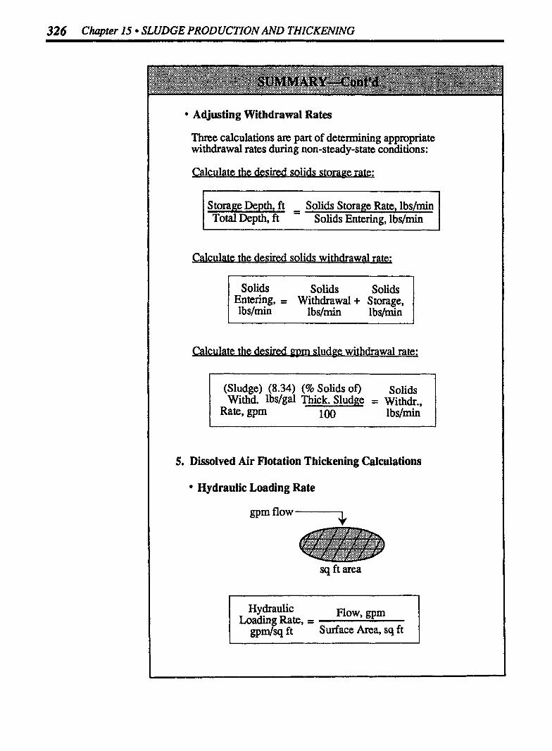
326 Chapter 15 SLUDGE PRODUCTION AND THICKENING
Adjusting Withdrawal Rates
Three calculations are part of determining appropriate withdrawal rates during non-S teady-S tate conditions:
Calculate the desired solids storage rate;
Storage Depth, ft - Solids Storage Rate, lbslmin - Total Depth, ft Solids Entering, lbs/min
l
Calculate the desired solids withdrawal rate; -
Solids Solids Solids Entering, = Withdrawal + Storage, l bs/min l bslrnin lbslmin
I Calculate the desired g m sludge withdrawal rate;
5. Dissolved Air Flotation Thickening Calculations
(Sludge) (8.34) (%I Solids of) Solids Withd. lbs/gal Thick. Sludge = With&,,
Rate, gpm 100 Ibs/min
Hydraulic Loading Rate
gpm flow 7
sq ft area
Hydraulic Flow, gpm Loading Rate, =
gpm/sq ft Surface Area, sq ft

Solids Loading Rate
lbs/hr solids ----If
sq ft area Sim~lified Eauation;
Ex~anded Eauation; I
(gpm) (60 min) (8.34) (%SS)
Solids Loading sludge 7 l b s f g a l x Rate, lbs/hr/sq ft = flow
Area, sq ft
Air Applied
Air, (Air, cfm)(60 rmn)(0.075 ibs) lbsfhr hr cu ft
AidSo1id.s Ratio
lifecl Equation;
Airjsolids Air, lbs/min Ratio - Solids, lbslmin
Expanded Eauation:
AirfSolids (cfm Air) (0.075 lbslcu ft) Ratio (gpm) (8.34) (% SS)
Sludge lbslgal 100
Percent Recycle Rate
Recycle Flow, gprn Recycle, % =
Sludge Flow to DAF-Unit, gpm I

328 Chapter I5 SLUDGE PRODUCTION AND THICKENING
Solids Removal Efficiency
v mglL Solids Removed
Solids Removal Solids Removed, mg/L % Solids in Influent, mglL
Concentration Factor
Concentration - - Thickened Sludge Conc., % Factor Influent Sludge Conc., %
6. Centrifuge Thickening Calculations Hydraulic Loading Rate- Scroll or Disc Centrifuges
Hydraulic - Flow, gpd Loading, @h - 24 hrdday
Hy&aulic = @W, gprn )(60 min) Loading, gph hr
Hydraulic Loading Rate- Basket Centrifuges
simplified Eauation:
Hydraulic - (gph) (Duration of Sludge Flow) I badin& @h flow Time in Operation
I Ex~anded Eauation:
Hydraulic - (gpm) (60 - min) @ur. of Sludge Flow) I b d n & - flow h, = h e in Operation
l - Hydraulic - - (gpd flow) (Dur. of Sludge HOW) Loading, g'Ph 24 hrs/day Time in Operation

Solids Loading Rate-Scroll or Disc Centrifuges
The equation used depends on how the flow rate is l expressed:
Solids Loading, = (8.34) (96 Solids) lbslhr sludge lbs/gal 1 0
flow
solids Loading, = (@m) (60 d n ) (8.34) (% Solids) lbs/hr sludge hr lbs/gal 1 0
flow
I . Solids Loading Rate-Basket Centrifuges Solids loading rates for basket centrifuges are calculated the same as for scroll or disc centrifuges except that the flow rate must be adiusted for the actual duration of sludge flow to the unit.
I Feed Time (Fill Time) for Basket Centrifuges
I Sim~lified Equation;
Fill Time, - S t o ~ d Solids Capacity, lbs Solids Entering, lbs fmin
I Expanded Eauation;
(Basket) (7.48) (8.34) (46 Basket Solids) Capac.; g&u ft lbslgal 1 Fill Time, cu ft loo . - -
(gpm) (8.34) (% Influent Solids) sludge lbs/gal 100
flow I
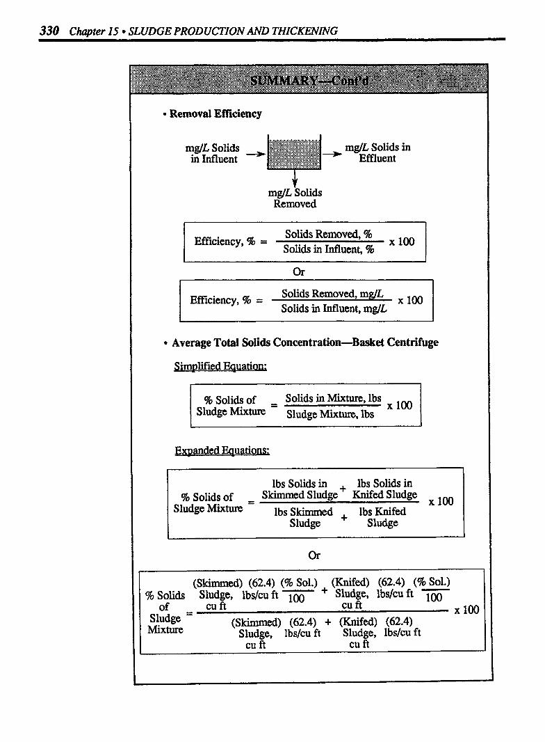
330 Chapter 15 SLUDGE PRODUCTION AND THICKENNG
Removal Effciency
mglL Solids Removed
Efficiency, % = Solids Removed, % Solids in Influent, %
x l M I Solids Removed, mglL Efficiency, % = Solids in Influent, mglL
Average Total Solids Concentration-Basket Centrifuge
Sim~lified Eauation;
% Solids of - Solids in Mixture, lbs Sludge Mixture Sludge Mixture, lbs
Ex~anded Eauations; P-
lbs Solids in , lbs Solids in I % Solids of - - Skimmed Sludge ' Knifed Sludge
Sludge Mixture lbs Skimmed . lbs Knifed
I Sludge Sludge I
(Skimmed) (62.4) (% Sol.) (Knifed) (62.4) (% Sol.) - % Solids Sludge, lbs/cu ft 100 + Sludge, lbslcu ft
of cu ft cu ft X l o o Sludge - Mixture (Skimmed) (62.4) + (Knifed) (62.4)
Sludge, lbslcuft Sludge, lbslcuft cu ft cu ft


332 Chapter 15 SLUDGE PRODUCTION AND THICKENING
15.1 PRIMARY & SECONDARY CLARIFIER SOLIDS PRODUCTION
CALCULATING SOLIDS PRODUCED- PRIMARY SYSTEM
The solids produced during primary treatment depends on the solids that settle in, or are removed by, the clarifier.
Use the mglL to lbs/day equation* to determine the lbs/day solids removed by the clarifier:
(mglL) (MGD) ( 8.34 ) = lbs/day SS flow lbslgal SS
Rem. Rem.
When making calculations pertaining to solids and sludge, remember that the term "solids" refers to dry solids and the term "sludge" refers to the solids and water.
Example 1: (Solids Production) Q A primary clarifier receives a flow of 1.82 MGD with a suspended solids concentration of 345 mglL. If the clarifier effluent has a suspended solids concentration of 190 mglL, how many pounds of solids are generated daily?
(mglL SS) (MGD flow) (8.34 lbs/gal) = lbs/day SS Removed Removed
(155 mglL) (1.82 MGD) (8.34 lbslgal) = 1 2353$:%&~ I
Example 2: (Solids Production) C3 The suspended solids content of the rim influent is 360 mglL and the primary effluent is 2 d' 8 mg/ ? How many pounds of solids are produced during a day that the flow is 4,220,000 gpd?
Complete the lbslday calculation:
(mg/L SS) (MGD flow) (8.34 lbslgal) = lbslday SS Removed Removed
I 5350 lbslday / (152 mglL) (4.22 MGD) (8.34 lbslgal) = Solids Removed
* Refer to Chapter 3 for a review of mg/L to lbs/day calculations.
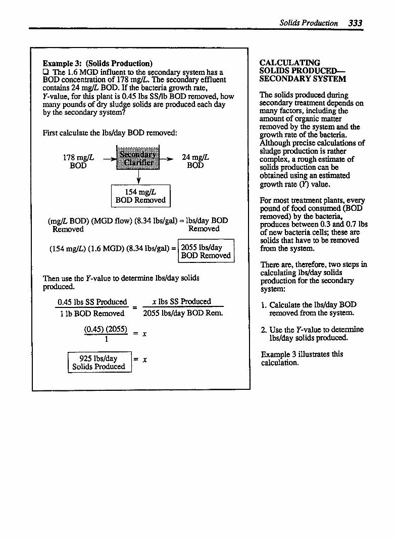
Solids Production 333
Example 3: (Solids Production) Ll The 1.6 MGD influent to the secondary system has a BOD concentration of 178 mglL. The secondary effluent contains 24 mglL BOD. If the bacteria growth rate, Y-value, for this plant is 0.45 lbs SS/lb BOD removed, how many pounds of dry sludge solids are produced each day by the secondary system?
First calculate the lbslday BOD removed:
(mg/L BOD) (MGD flow) (8.34 lbslgal) = lbslday BOD Removed Removed
(1 54 mg/L) (1.6 MGD) (8.34 lbslgal) = 2055 lbs/day I BOD Removed 1 Then use the Y-value to determine lbslday solids produced.
0.45 lbs SS Produced - - x lbs SS Produced 1 lb BOD Removed 2055 lbslday BOD Rem.
Solids Produced
CALCULATING SOLIDS PRODUCED- SECONDARY SYSTEM
The solids produced during secondary treatment depends on many factors, including the amount of organic matter removed by the system and the growth rate of the bacteria. Although precise calculations of sludge production is rather complex, a rough estimate of solids production can be obtained using an estimated growth rate (Y) value.
For most treatment plants, every pound of food consumed (BOD removed) by the bacteria, produces between 0.3 and 0.7 lbs of new bacteria cells; these are solids that have to be removed from the system.
There are, therefore, two steps in calculating lbsfday solids production for the secondary system:
1. Calculate the lbslday BOD removed from the system.
2. Use the Y-value to determine lbslday solids produced.
Example 3 illustrates this calculation.

334 Chapter 15 SLUDGE PRODUCTION AND THICKENMG
15.2 PERCENT SOLIDS AND SLUDGE PUMPING
PERCENT SOLIDS
Sludge is comprised of water and solids. The vast majority of sludge is water-usually in the range of 93% to 97%.
To determine the solids content of a sludge, a sample of sludge is dried overnight in an oven at 103'- 105' C. The solids that remain after drying represent the total solids content of the sludge. This solids content may be expressed as a percent or as a mglL concentration.** Two equations are used to calculate percent solids, depending on whether lab data or plant data is used in the calculation. In both cases, the calculation is on the basis of solids and sludge weight:
-
Total Solids, g % Solids =
Sludge Sample, g X 100
Solids, lbslday 96 Solids =
Sludge, lbslday
Example 1: (Percent Solids and Sludge Pumping) O The total weight of a sludge sam le is 20 grams. (Sludge sample only, not the dish.) P f the weight of the solids after drying is 0.58 grams, what is the percent total solids of the sludge?
% Solids = Total Solids, grams Sludge Sample, grams
- - 0.58 grams 20 grams
X loo
Example 2: (Percent Solids and Sludge Pumping) P A total of 4100 gallons of slud e is pumped to a digester daily. If the sludge has a 8 % solids content, how many lbslday solids are pumped to the digester? (Assume the sludge weighs 8.34 lbdgal.)
First, write the percent solids equation and fill in the given information:
% Solids = Solids,lbs/day Sludge, lbslday
- - X lbslday Solids (4 100 gal) (8.34 lbs/gal)
1710 lbslday Solids
* This graphic is to illustrate the composition of sludge. Under normal circumstances, of course, the solids and water are mixed.
** 1% solids = 10,000 mg/L. For a review of % to mg/L conversions, refer to Chapter 8.

56 Solids and Sludge Pumping 335
Example 3: (Percent Solids and Sludge Pumping) D A total of 8,700 lbslday SS are removed from a primary clarifier and pumped to a sludge thickener. If the sludge has a solids content of 2.596, how many lbs/day sludge are pumped to the thickener?
% Solids = Solids, lbs/&y 1100 Sludge, lbs/day
2.5 = 8,700 lbsfday Solids ,100 x lbs/day Sludge
Example 4: (Percent Solids and Sludge Pumping) O It is anticipated that 320 lbs/&y SS will be pumped from the primary clarifier of a new plant. If the primary clarifier sludge has a solids content of 4.5%, how many gpd sludge will be pumped from the clarZer? (Assume the sludge weighs 8.34 lbs/gal.)
First calculate lbs/day sludge to be pumped using the % solids equation, then convert lbslday sludge to gpd sludge:
lbs/day Sludge = Solids, lbs/day % Solids
x lbs/day Sludge = 320 lbs/&y Solids 0.045
Converting lbslday sludge to gpd sludge:
7llllbs/daySludge - 853 gpd 8.34 lbs/gal - / Sludge I
CALCULATING OTHER UNKNOWN VARIABLES
The three variables in percent solids calculations are percent solids, lbs/day solids, and lb-y sludge. In Example 1 percent solids was the unknown variable. Examples 2-4 illustrate calcu- lations when other variables are unknown. To solve these pro- blems, write the equation as usual, fill in the known infor- mation, then solve for the m- known value.*
SLUDGE TO BE PUMPED
As mentioned above, one of the variables in the percent solids calculation is lbs/day sludge. Example 3 illustrates a calculation of lbs/day sludge. Example 4 illustrates the calculation of gpd sludge to be pumped.
Because lbs/&y sludge is calculated relatively frequently, the percent solids equation is often rearranged as follows:
l Sludge, = Solids, lbs/dW lbslday % Solids
* Refer to Chapter 2 in Basic Math Concepts for a review of solving for the unknown factor.

336 Chapter 15 SLUDGE PRODUCTION AND THICKENING
15.3 THICKENING AND SLUDGE VOLUME CHANGES
Sludge thickening calculations are based on the concept that the solids in the primary or secondary sludge are equal to the solids in the thickened sludge. The solids are the same.* It is primarily water that has been removed in order to thicken the sludge and result in a higher percent solids. In the unthickened sludge, the solids might represent 1 or 4% of the total pounds of sludge. But when some of the water is removed, that same amount of solids might represent 5-7% of the total pounds of sludge.
Because the pounds of solids remain unchanged, when making sludge thickening calculations, the lbslday solids of the unthickened sludge may be set equal to the lbslday solids of the thickened sludge, as shown to the right.
Normally the lbs/day solids are not known directly but must be calculated, based on lbslday (or gpd) sludge and percent solids content of that sludge, as shown in the expanded equation.
Note that both the primary or secondary sludge and the thickened sludge are assumed to have a density of 8.34 lbslgal). The actual density of the sludge should be determined and used if it is different than 8.34 lbslgal. The density of the primary or secondary sludge may be different than the thickened sludge density. Refer to Chapter 7, Section 7.1, "Density and Specific Gravity".
THE KEY 'I0 SLUDGE THICKENING CALCULATIONS-SOLIDS REMALN CONSTANT*
Unthickened S ludee
l Sludge
Simplified Equation:
lbs Solids , lbs Solids in Unthickened Sludge in Thickened Sludge
Expanded Equations:
(Rim. or Sec) (% Solids) - (Thickened) (% Solids) - Sludge, 100 sludge, 100 lbsfday lbsfday
(Prim. or Sec.). (8.34) (95 Solids) = (Thickened) (8.34) (% Solids) sludge, gpd lbsfgal 100 Sludge, gpd lbslgal 100
Example 1: (Sludge Thickening) A primary clarifier sludge has a 3% solids content. A total
of 25,400 lbslday sludge is pumped to a thickener. If the sludge has been concentrated to 5% solids, what will be the expected lbslday sludge flow from the thickener?
(Primary) (% Solids) - - (Thickened) (% Solids) Sludge, 100 Sludge, lbslday l b slday
* This assumes a negligible amount of solids are lost in the thickener overflow.
15,240 lbs/day Thickened Sludge
- X

Sludge Thickening 337
Example 2: (Sludge Thickening) P A primary clarifier sludge has a 3.2% solids content. If 3140 gpd pnmary sludge is pumped to a thickener and the thickened sludge has a solids content of 5.896, what would be the expected gpd flow of thickened sludge? (Assume both sludges weigh 8.34 lbs/gal.)
Since sludge data is given as gpd, the second expanded equation is used:
(Prim. or Sec.) (8.34) (% Solids) - - (Thickened) (8.34) (% Solids) Sludge, gpd lbs/gal Sludge, gpd lbs/gal 100
Fill in the given information and solve for the unknown value:
Example 3: (Sludge Thickening) O The sludge from a primary clarifier has a solids content of 2.8%. The primary sludge is pumped at a rate of 45 10 gpd to a thickener. If the thickened sludge has a solids content of 5.2%, what is the anticipated gpd sludge flow from the thickener? (Assume both sludges weigh 8.34 lbslgal.)
1732 gpd Thickened Sludge
(Prim. or Sec.) (8.34) (% Solids) , (Thickened) (8.34) (% Solids) Sludge, gpd lbs/gal Sludge, gpd lbdgal
= X
(45 10 gpd) (m) (0.028) W) (0.052)
= X
2428 gpd Thickened Sludge = X
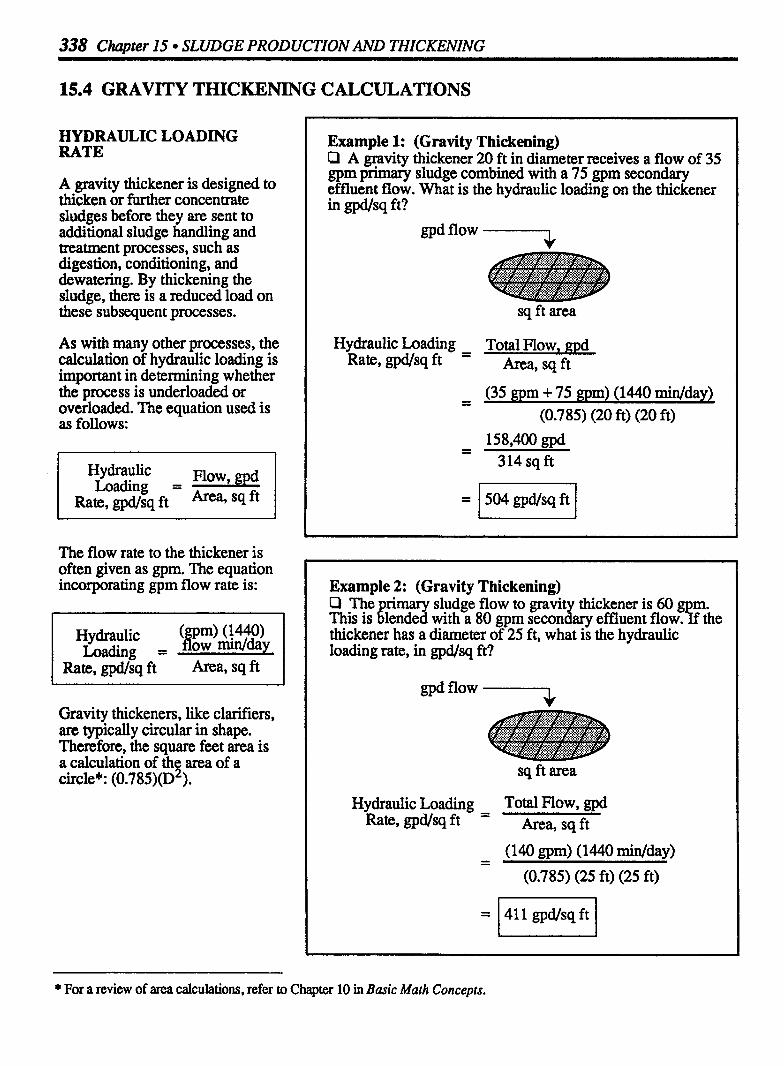
338 Chapter 15 SLUDGE PRODUCTION AND THICKENING
15.4 GRAVITY THICKENING CALCULATIONS
HYDRAULIC LOADING RATE
A gravity thickener is designed to thicken or further concentrate sludges before they are sent to additional sludge handling and treatment processes, such as digestion, conditioning, and dewatering. By thickening the sludge, there is a reduced load on these subsequent processes.
As with many other processes, the calculation of hydraulic loading is important in determining whether the process is underloaded or overloaded. The equation used is as follows:
H~haulic - Flow, gpd Loading -
Rate, gpd/sq ft Area, sq ft
The flow rate to the thickener is often given as gpm. The equation incorporating gprn flow rate is:
Hydraulic (prn) Loading = ow mdday
Gravity thickeners, like clarifiers, are typically circular in shape. Therefore, the square feet area is a calculation of thej area of a circle*: (0.785)@ ).
Example 1: (Gravity Thickening) P A gravity thickener 20 ft in diameter receives a flow of 35 gprn primary sludge combined with a 75 gpm secondary effluent flow. What is the hydraulic loading on the thickener in gpd/sq ft?
gpd flow 7
Hydraulic Loading - Rate,gpd/sqft -
sq ft area
Total Flow, gpd Area, sq ft
(35 gpm + 75 gpm) (1440 midday) (0.7 85) (20 ft) (20 ft)
158.400 md
Example 2: (Gravity Thickening) O The rimary sludge flow to gravit thickener is 60 n This is lended with a 80 gpm secon K ary effluent flow% the thickener has a diameter of 25 ft, what is the hydraulic loading rate, in gpd/sq ft?
gpd flow 7
sq ft area
Hydraulic Loading - Total Flow, Rate, gpd/sq ft - Area, sq ft
- - (140 gpm) (1440 midday)
(0.785) (25 ft) (25 ft)
* For a review of area calculations, refer to Chapter 10 in Basic Math Concepts.
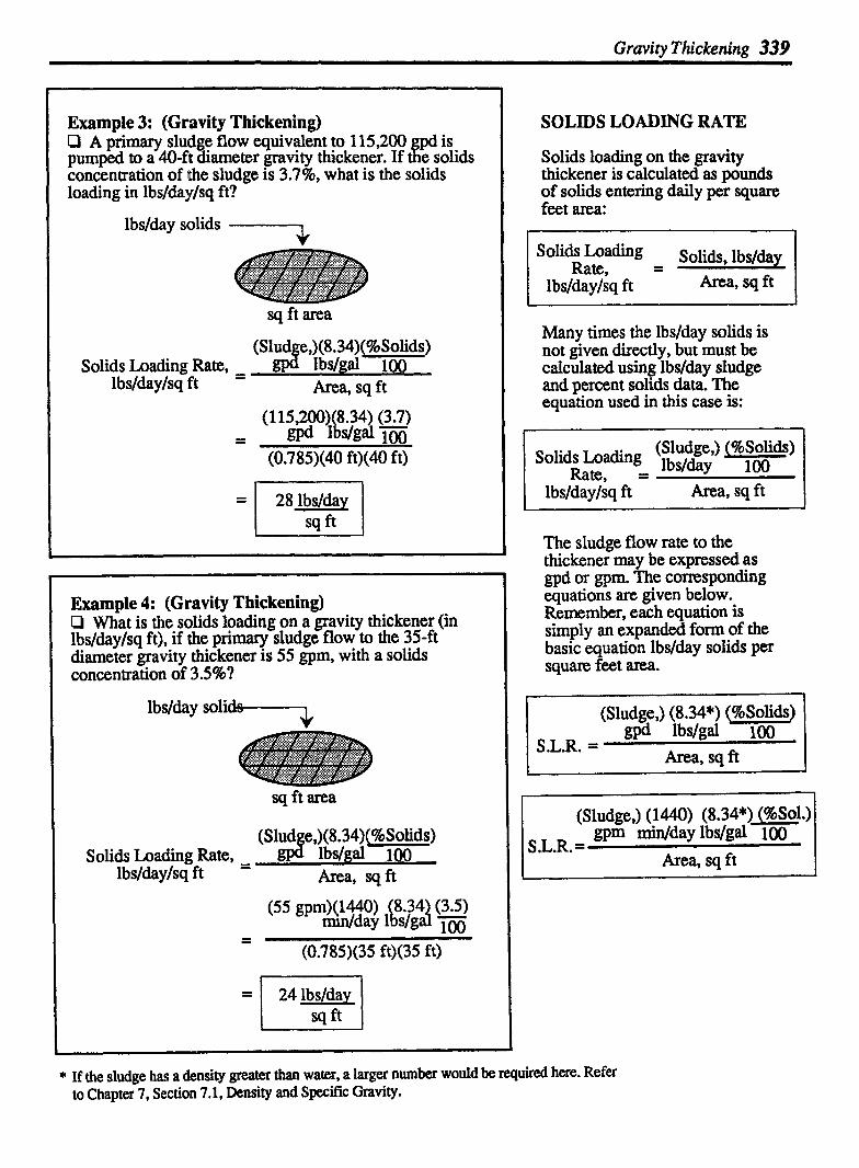
Graviry Thickening 339
Example 3: (Gravity Thickening) P A primary sludge flow equivalent to 115,200 pumped to a 40-ft diameter gravity thickener. If Fd e solids is concentration of the sludge is 3.796, what is the solids loading in lbs/&y/sq ft?
lbslday solids 7
sq ft area
(Slud e,)(8.34)(%Solids) Solids Loading Rate, -
lbs/&y/sq ft - lid Wgal 100
Area, sq ft
- - (0.785)(40 ft)(40 ft)
Example 4: (Gravity Thickening) P What is the solids loading on a gravity thickener (in Ibs/day/sq ft), if the primary sludge flow to the 35-ft diameter gravity thickener is 55 gpm, with a solids concentration of 3 S%?
sq ft area
(Slud e,)(8.34)(%Solids) Solids Loading Rate, - gP 8 Wgal 100
lbs/daylsq ft - Area, sq ft
- -
(0.785)(35 ft)(35 ft)
SOLIDS LOADING RATE
Solids loading on the gravity thickener is calculated as pounds of solids entering daily per square feet area:
lbsldaylsq ft Area, sq ft
Many times the lbslday solids is not given directly, but must be calculated using lbslday sludge and percent solids data. The equation used in this case is:
(Sludge,) (%Solids) Solids Loading lbs/day Rate, = 100
lbs/day/sq ft Area, sq ft
The sludge flow rate to the thickener may be expressed as gpd or gpm. The corresponding equations are given below. Remember, each equation is simply an expanded fonn of the basic equation lbslday solids per square feet area.
S.L.R. =
(Sludge,) (8.34*) (%Solids) gpd Wgal 100
Area, sq ft
(Sludge,) (1440) (8.34*) (%sol.) gpm min/day lbdgal
S.L.R. = Area, sq ft I
* If the sludge has a density greater than water, a larger number would be required here. Refer to Chapter 7. Section 7.1. Density and Specific Gravity.
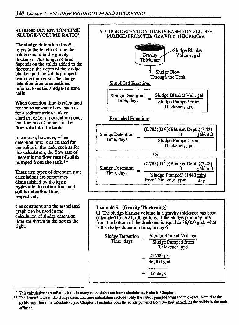
340 Chapter 15 SLUDGE PRODUCTION AND THICKENING
SLUDGE DETENTION TIME (SLUDGE-VOLUME RATIO)
The sludge detention time* refers to the length of time the solids remain in the gravity thickener. This length of time depends on the solids added to the thickener, the depth of the sludge blanket, and the solids pumped from the thickener. The sludge detention time is sometimes referred to as the sludge-volume ratio.
When detention time is calculated for the wastewater flow, such as for a sedimentation tank or clarifier, or for an oxidation pond, the flow rate of interest is the flow rate into the tank.
In contrast, however, when detention time is calculated for the solids in the tank, such as for this calculation, the flow rate of interest is the fiow rate of solids pumped from the tank.**
These two types of detention time calculations are sometimes distinguished by the terms hydraulic detention time and d i d s detention time, respectively . The equations and the associated graphic to be used in the calculation of sludge detention time are shown in the box to the right
SLUDGE DETENTION TIME IS BASED ON SLUDGE PUMPED FROM THE GRAVITY THICKENER
v Sludge Flow Through the Tank
simplified Eauation;
Sludge Detention - Sludge Blanket Vol., gal Time, days - Sludge Pumped from
Thickener, gpd
Expanded Equation;
(0.785)(D2 )(Blanket Depth)(7.48) Sludge Detention - ft gucu ft Time, days - Sludge Pumped from
Thickener, gpd
I Sludge Detention m:-- -l_---
- ft gucu ft I
I 1 me, aays (Sludge Pumped) (1440 min) I frc m Thickener, gpm by 1
Example 5: (Gravity Thickening) C l The sludge blanket volume in a vity thickener has been r calculated to be 21,700 gallons. If e sludge pumping rate from the bottom of the thickener is equal to 36,000 gpd, what is the sludge detention time, in days?
Sludge Detention - Time, days
Sludge Blanket Vol., gal Sludge Pumped from
Thickener, gpd
21,700 gal 36,000 gpd
10.6 days I
* This calculation is similar in form to many other detention time calculations. Refer to Chapter 5. ** The denominator of the sludge detention time calculation includes only the solids pumped from the thickener. Note that the
solids retention time calculation (see Chapter 5) includes both the solids pumped from the tank well the solids in the tank effluent .

Gravity Thickening 341
Example 6: (Gravity Thickening) Cl A gravity thickener 40-ft in diameter has a sludge blanket depth of 3.2 ft. If sludge is pumped from the bottom of the thickener at the rate of 20 gpm, what is the sludge detention time (in days) in the thickener? (Assume the pumping rate is continuous.*)
Sludge - Sludge Blanket Vol., gal Detention - Sludge Pumped fiom Time, days Thickener, gpd
- - (0.785)(40 ft)(40 ft)(3.2 ft)(7.48 gal/cu ft) (20 gpm)(1440 min/day)
30,064 gal - 28,800 gpd
= I 1.0 days I
Example 7: (Gravity Thickening) D A gravity thickener 35 ft in diameter has a sludge blanket depth of 3.8 ft. If the sludge is pumped from the bottom of the thickener at a rate of 25 gpm, what is the sludge detention time, in hours, in the thickener? (Assume the pumping rate is continuous.)
Sludge - Sludge Blanket Vol., gal Detention Sludge Pumped from Time, hrs Thickener, gph
- - 27,333 gal l500 gph
= 1 18.2 hrs I
SLUDGE DETENTION TIME EXPRESSED IN HOURS
For detention times less than one day, it may be desirable to express the detention time in hours. If so, the pumping rate must also be expressed in terms of gallons per hour:
I Sludge Blanket I Sludge - vol., gal
Detention Pumping Rate, Time, hours @h
Sludge Blanket Sludge Vol., gal
Detention - (Pumping)(60) Time, hours Rate, min/hr
Example 7 illustrates this type of calculation.
* If the pumping rate were not continuo~, you would use a different conversion factor than 1440 midday to convert to gpd pumped. The factor to be used would be the total number of minutes pumped during the day.

342 Chapter I5 SLUDGE PRODUCTION AND THICKENING
EFFICIENCY
The efficiency of a gravity thickener is a measure of the effectiveness in removing suspended solids from the flow. As with other calculations of efficiency*, the calculation includes amount removed divided by the total amount:
Total
In calculations of gravity thickener efficiency, the percent sludge solids (% SS) removed is determined using the equations given below.
1 % SS Removed 100
% SS in Influent
This equation can be simplified by dividing out the hundreds in the numerator and denominator of the fraction:
~f f ic . , = SS Removed, % I % SS in Influent, % 1001
The percent sludge solids may also be expressed as mg/L** to calculate efficiency:
Examples 8 and 9 illustrate efficiency calculations.
Example 8: (Gravity Thickening) O The sludge flow entering a gravity thickener contains 3.1 % solids. The effluent from the thickener contains 0.18% solids. What is the efficiency of the gravity thickener in removing solids?
t 2.92 % Solids
Removed
Efficiency, % = % SS Removed % SS in Influent
= - 2*92 X 100 3.1
Example 9: (Gravity Thickening) P What is the efficient of the gravi thickener if the influent flow to the thic l ener has a so TY ids concentration of 2.8%, and the effluent flow has a solids concentration of 0.7961 Calculate the efficiency using mg/L solids concentration.
First convert the data from percent to mglL (1% = 10,000 mg/L):
2.8% = 28,000 mg/L 0.7% = 7,000 mg/L
Efficiency, % = 21,000 mg,& 28,000 mg/L
* For a review of other types of efficiency calculations, refer to Chapter 6. ** For a discussion of m@ to percent conversions. refer to Chapter 8 in Bmic Moth Concepts.

Gravity Thickening 343
Example 10: (Gravity Thickening) O The sludge solids concentration of the influent flow to a gravity thickener is 3.2%. If the sludge withdrawn from the bottom of the thickener has a sludge solids concentration of 8%, what is the concentration factor?
Concentration - Thickened Sludge, % Factor Influent Sludge, %
Example 11: (Gravity Thickening) O The influent flow to a vity thickener has a sludge solids concentration of 3 r h h a t is the concentration factor if the sludge solids concentration of the sludge withdrawn from the thickener is 8.7%?
Concentration - Thickened Sludge, % Factor Influent Sludge, %
CONCENTRATION FACTOR
The concentration factor is another means of determining the effectiveness of the gravity thickening process.
The concentration factor indicates how much the sludge has been concentrated as a result of the thickening process. For example, a concentration factor of 2 means that after thickening the sludge is twice as concentrated as when it entered the thickener, a concen- tration factor of 3 indicates that the thickened sludge is three times as concentrated as when it entered the thickener, etc.
To determine the concentration factor, simply compare the thickened sludge concentration with the influent sludge concentration:
Concent. Thickened Sludge, % Factor - Influent Sludge, %

344 Chupter 15 SLUDGE PRODUCTION AND THICKENING
SOLIDS BALANCE AT THE THICKENER
Monitoring the solids entering and leaving the gravity thickener, as well as those retained in the thickener (sludge blanket) is essential in the effective operation of the process.
When determining the solids balance (mass balance) at the thickener, the solids entering the thickener are compared with those leaving the system (either through the underflow as thickened sludge, or in the effluent). The balance between incoming and outgoing solids determines whether the sludge blanket will increase, decrease, or stay the same.
If the solids going in equal the solids going out, the sludge blanket level wiU stay the same. For example, if 40,000 lbslday solids leave the thickener (in underflow and overflow), there are no additional solids being stored:
Solids = Solids + Solids In Out S tored
40,000 = 40,000 + 0 lbslday lbslday lbslday
If the solids going in are greater than the solids going out, the sludge blanket level will begin to rise. For example, if 40,000 lbslday solids enter the thickener and only 30,000 lbslday leave the thickener, then 10,000 lbslday will be stored in the sludge blanket:
Solids = Solids + Solids In Out S tored
40,000 , 30,000 + 10,000 lbs/day lbslday lbslday
SOLIDS BALANCE COMPARES SOLIDS IN WITH SOLIDS OUT AND SOLIDS STORED
Solids In, lbdday
solids Out in Underflow, lbs/day (Thickened Sludge)
Simplified Equation:
Solids In, = Solids Out Solids Out Solids in Underflow, + in Effluent,+ Stored lb 'lday (Thickened Sludge) lbslday lbs/day
lbs/dav
Expanded Equation:*
Solids In, = Solids Out Solids Out Solids lbs/day in Underflow, + in Effluent, + Stored
l l b slday lbslday lbsld I I I
(Sludge Pumped) (1440**) (8.34)(7 . I to thickener minfday ibslgal 100 OSol)l I
( Sludge ) (1440) (8.34) (% Sol.) Withdrawn min/day lbslgal 100
a?*
(Effluent) (1440) (8.34)W Flow,gpm min/day lbslgd 100
O s o l * I I P - 1 (0.785)@) (depth) (7.48) (8.34)
ft/day gaVcu ft lbs/gal I
* Note that each of these lbs/day quantities may be calculated using mg/L concentration rather than percent. In that case, the calculation would be (mglL solids)(MGD flow)(8.34 lbqgal). The result will be the same. Refer to Chapter 8 in Basic Math Concepts for a review of mg/L and percent conversions.
** If the pumping is not continuous, use the total number of minutes pumped per day rather than the 1440 midday factor.

Graviv Thickening 345
Example 12: (Gravity Thickening) O Given the data below, (a) determine whether the sludge blanket in the gravity thickener will increase, decrease, or remain the same; and (b) if there is an increase or decrease, how many lbslday solids change will this be?
Sludge Pumped to Thickener = l l0 gprn Thickened Sludge Pumped from Thickener = 50 gprn Primary Sludge Solids = 3% Thickened Sludge Solids = 8% Thickener Effluent Suspended Solids = 600 mglL
a) First, determine lbdday sludge solids entering the thickener. (1 10 gpm) (1440 midday) (8.34 lbslgal) ( - 3 ) = 39,632
loo lbsl&y
Next, calculate lbs/day sludge solids leaving the thickener via the underflow: (50 gpm) (1440 min/day) (8.34 lbslgal) ( - 8 ) = 48,038
100 lbs/&y
And the lbs/&y sludge solids leaving the thickener via the effluent flow:* (The effluent flow is l l0 gpm - 50 gprn = 60 gpm. Also, 600 m@L = 0.06%)
(60 gpm) (1440 midday) (8.34 lbslgal) (0.06) = 432 - 100 lbslday
To summarize the sludge solids entering and leaving:
39,632 432 lbslday l bs/day leaving via entering 7 Thickener effluent,
48,038 lbs/day leaving via underflow
As indicated by the diagram, there are more solids leaving the thickener than entering. Therefore the sludge blanket level will drop*
b) The lbs/day drop in level depends on the difference between solids entering and leaving the thickener:
48,470 Total - 39,632 lbslday = 1 1:; 1 lbs/day leaving entering lbslday
If the solids going in are less than the solids going out, the sludge blanket level will begin to fall. For example, if 35,000 lbs/day solids enter the thickener and 40,000 lbs/&y leave the thickener, then the sludge blanket will fall an equivalent of 5,000 lbs/day :
Solids In = Solids Out + Solids Stored
In Example 12, there is a comparison of solids entering and leaving the thickener. The effect on the sludge blanket level is also calculated.
Although the equation shown in Example 12 includes solids in the thickener effluent, these solids are sometimes considered negligible (that is, they have little effect on the overall calculation) provided the effluent contains a solids concentration less than 500 mglL and there is little solids carry over in the effluent.
* The lbslday solids may be calculated using the flow and percent solids, as shown in the calculation of solids entering the digester; or, the lbs/day solids may be calculated using mglL concentration-(mg/L)(Flow. MGDI(8.34 lbs/gal) = Ibs/day.

346 Chapter 15 SLUDGE PRODUCTION AND THICKENNG
TIME REQUIRED FOR SLUDGE BLANKET RISE OR FALL
Once you have determined the sludge storage rate, as illustrated in Example 12, you can determine the time nquired for the sludge blanket to reach a desired level.
This calculation is similar to a detention time or fill-time calcu- lation,* as shown to the right. As with all detention time calcula- tions, if the time is desired in hours, the flow rate (or storage rate in this calculation) must be expressed in corresponding time units-lbs~hr.
Flow conversions from one unit to another may be required in these calculations. For a review of flow conversions, refer to Chapter 8 in Basic Math Concepts.
RISE OR FALL TIME IS SIMILAR TO A DETENTION TIME CALCULATION
Desired Rise or Fall in Sludge Blanket Level
Sludge Blanket
For detention time, the volume and flow rate are generally expressed as gallons and gal/hr (or gal/min, etc.).-For rise or fall time, the solids and flow rate are expressed as lbs - and lbsfhr, respectively:
Simplified Equation:**
Rise or Fall Solids in Rise or Fall, lbs - Time, - Solids Storage Rate, lbs/hr
Expanded Equation:
(0.785)@2 )(Rise or Fall) 7.48 (8.34) (96 Sol.) I Rise or Fall Depth, ft g & cu 1 t lbsfgal ~IK) - - - v
Solids Storage Rate, lbs/hr
Example 13: (Gravity Thickening) O If solids are being stored at a rate of 8800 lbs/day in a 20-ft diameter gravity thickener, how many hours will it take the sludge blanket to rise two feet? The solids concentration of the thickened sludge is 7%.
Rise Time, (0.785)(D2)(Rise, ft) (7.48) (8.34) (% Sol.)
galfcu ft lbs/gal 100 - - -- - - hrs - Solids Storage Rate, lbsfhr
Before filling in the equation, the storage rate must be expressed as lbs/hr: 8800 lbsfday t 24 hrslday = 367 l b s h
(0.785) (20 ft) (20 ft) (2 ft) (7.48) (8.34) (7J Rise Time, 100
hrs = 367 lbs/hr
=l 7.5 hrs I
* For a review of detention time calculations, refer to Chapter 5. ** Note that the sludge blanket volume, rise or fall, must be expressed as pounds of solids
(rather than pounds of sludge) since the storage rate, lbsfmin or l b m is expressed in terms of solids.

Gravity Thickeninn 347
Example 14: (Gravity Thickening) P After several hours of startup of a gravit thickener, the sludge blanket level is mcasurul at 2.5 r t. The desired sludge blanket level is 6 ft. If the sludge solids are entering the thickener at a rate of 40 lbslmin, what is the desired sludge withdrawal rate, in gpm? The thickened sludge solids concentration is 6%.
First calculate the desired solids storage rate, using the ratio of stored (or current) to total sludge blanket depth:
Storage Depth, ft Solids Storage Rate, lbs/min -- -- p
Total Depth, ft solids Entering, lbsfrnin
Solids Storage Rate =L Next, calculate the solids withdrawal rate necessary to achieve the 17 lbslmin solids storage rate:
Solids - Solids + Solids Entering - Withdrawal, Storage, lbslmin lbs/rnin lbslmin
--
23 lbsfmin Solids Withdrawal Rate r
Then calculate the gpm sludge withdrawal rate that will result in withdrawing 23 lbs/min solids withdrawal:
(Sludge) (8.34) (% Sol. of) = Solids Withd., lbslgal Thickened S1. Withd., gPm 100 Ibs/min
(X gpm) (8.34) 6 ) = 23 lbslmin lbs/gal 100
ADJUSTING WITHDRAWAL RATES
Under continuous operation, the sludge blanket should be main- tained at a relatively constant level. The sludge withdrawal rates are generally not adjusted man than about 20% at a time.
During such times as startup, however, the withdrawal rate is sometimes adjusted significantly more than 20 percent to achieve an increase in sludge blanket depth. An appropriate sludge withdrawal rate in this situation may be determined using three steps: 1. Calculate the desired solids
storage rate, lbslmin, using the ratio* of the storage depth (current sludge blanket depth) to the total desired depth:
Storage Solids Storage Rate, Depth,= lbslmin
Total Solids Entering, Depth, ft lbslmin
2. Once the desired solids storage rate has been calculated, the desired soiids withdrawal rate, lbs/min, may be determined using the equation, solids in equal solids out plus solids stored:
Solids - Solids + Solids Withdrawal, Storage,
lbslmin lbslmin lbs/min -
3. This withdrawal rate may then be expressed as gpm sludge withdrawal rate:
(Sludge) (8.34) (% Sol. of) = Solids Withd., lbs/gal Thick. S1. Withd,
100 lbs/min
Withdrawal rate calculations m often made every few hours to verify sludge storage and sludge blanket changes.
* For a review of ratios and proportions, refer to Chapter 7 in Basic Math Concepts.

348 Chapter I5 SLUDGE PRODUCTION AND THICKENING
15.5 DISSOLVED AIR FLOTATION THICKENING CALCULATIONS
HYDRAULIC LOADING RATE
The hydraulic loading calculation for dissolved air flotation (DAF) thickeners is similar to other calculations of hydraulic loading-flow rate per surface area. For DAF thickeners, hydraulic loading is expressed as gpm/sq ft:
Hydraulic Loading Rate, = Flow, gprn
g~m/sq ft Surface Area, sq ft
Example l: (DAF Thickening) P A dissolved air flotation unit receives a sludge flow of 800 gprn. If the DAF unit is 50 ft in diameter, what is the hydraulic loading rate, in gpdsq ft?
gprn flow .1.
sq ft area
Hydraulic HOW, gprn Loading Rate, =
g p d q fi sq ft
- - 800 gprn (0.785)(50 ft)(50 ft)
Example 2: (DAF Thickening) Cl A dissolved air flotation unit is 45 ft lon and 15 ft 9 wide. If the unit receives a sludge flow of 1 0,000 gpd, what is the hydraulic loading, in gpm/sq ft?
sq ft area
Flow, gpm Loading Rate, =
g ~ d s 9 f t Area, sq ft
118 gprn - (45 ft)(15 ft)

DAF Thickening 349
Example 3: (DAF Thickening) P The sludge flow to a dissolved air flotation thickener is 120 gpm, with a suspended solids concentration of 0.75%. If the DAF unit is 50 ft long and 15 ft wide, what is the solids loading rate in lbs/hr/sq ft?
l b s b solids ---
sq ft area
(120 gpm) (60 min) (8.34) (0.75) - - hr lbs/gal 100
(50 ft)(15 ft)
Example 4: (DAF Thickening) P The 0.13-MGD sludge flow to a 30-ft diameter dissolved air thickener has a suspended solids concentration of 8200 mg/L, what is the solids loading rate in lbs/hr/sq ft?
1bs/hr solids 7
First
sq ft area
calculate lbs/day/sq ft solids loading:
Solids Loading - (8200 mg/L) (0.13 MGD) (8.34 lbs/gal) - Rate, lbs/day/sq ft (0.785) (30 ft) (30 ft)
Then convert to lbs/hr/sq ft solids loading:
SOLIDS LOADING RATE
The solids loading rate for gravity thickeners is expressed in lbs/day/sq ft. For DAF thickeners, however, the solids loading rate is expressed as lbs/hr/sq ft.
Simplified Equation:
Expanded Equation:
(gpm) (60 min) (8.34) (%SS) SLR' sludge hr lbslgal 100 l b s b = flow Isq ft
Area, sq ft
Example 3 illustrates this calculation.
If the suspended solids concen- tration is expressed as m&* rather than percent, the following equation may be used to calculate solids loading rate as lbsldayfsq ft:
m L) (MGD) (8.34) SLR, - (g fl ow lbs/gal
lbsldayfsq fi Area, sq ft I
The solids loading rate can then be converted to lbs&/sq ft as follow S:
Example 4 illustrates this calculation.
* For a review of mg/L to lbs/&y calculations refer to Chapter 3. For a discussion of mglL and pcrcent conversions. refer to Chapter 8 in Basic Math Concepts.
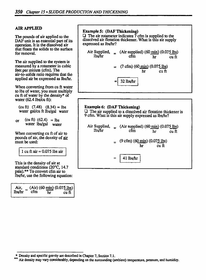
350 Chapter 15 SLUDGE PRODUCTION AND THICKENING
AIR APPLIED
The pounds of air applied to the DAF unit is an essential part of its operation. It is the dissolved air that floats the solids to the surface for removal.
The air supplied to the system is measured by a rotameter in cubic feet per minute (cfrn). The air-to-solids ratio requires that the applied air be expressed as lbs/hr.
When converting from cu ft water to lbs of water, you must multiply cu ft of water by the density* of water (62.4 lbslcu ft):
(cu ft) (7.48) (8.34) = lbs water gaVcu ft lbs/gal water
When converting cu ft of air to pounds of air, the density of & must be used:
1 1 cu ft air = 0.075 lbs air I This is the density of air at standard conditions (20°C, 14.7 psis).** To convert cfrn air to lbs/hr, use the following equation:
Air, (Ai.)(60min)(O.O751bs) lbs/hr = cfm h, cu ft
Example 5: (DAF Thickening) P The air rotameter indicates 7 cfm is su plied to the dissolved air flotation thickener. What is $S air supply expressed as lbs/hr?
Air Supplied, = (Air supplied) (60 min) (0.075 lbs) lbs/hr cfm hr cu ft
(7 cfm) (60 min) (0.075 lbs) hr cu ft
Example 6: (DAF Thickening) P The air supplied to a dissolved air flotation thickener is 9 cfm. What is this air supply expressed as lbs/hr?
Air Supplied, , (Air supplied) (60 min) (0.075 lbs) Ibs/hr cfm hr cu ft
- - (9 cfm) (60min) (0.075 lbs) hr cu ft
* Density and specific gravity are described in Chapter 7, Section 7.1. ** Air density may vary considerably, depending on the surrounding (ambient) temperature, pressure, and humidity.
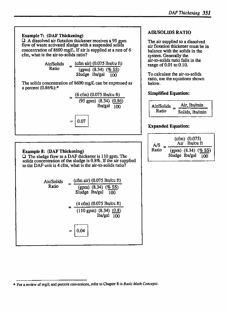
DAF Thickening 351
Example 7: (DAF Thickening) O A dissolved air flotation thickener receives a 95 m flow of waste activated sludge with a suspended soli 3 S concentration of 8600 mglL. If air is supplied at a rate of 6 cfm, what is the air-to-solids ratio?
Air/solids (cfm air) (0.075 lbslcu ft) - - Z
Ratio (gpm) (8.34) (% SS) Sludge lbslgal 100
The solids concentration of 8600 mglL can be expressed as a percent (0.86%):*
(6 cfm) (0.075 lbslcu ft) (95 gpm) (8.34) (0.86)
Wgal 100
Example 8: (DAF Thickening) P The sludge flow to a DAF thickener is 110 gpm. The solids concentration of the sludge is 0.8%. If the air supplied to the DAF unit is 4 cfm, what is the air-to-solids ratio?
Air/Soli& - - (cfm air) (0.075 ~ ~ S / C U ft) Ratio (gpm) (8.34) (% SS)
Sludge lbs/gal 100
(4 cfm) (0.075 lbs/cu ft) (1 10 gpm) (8.34) l0.8)
lbslgal
AIR/SOLIDS RATIO
The air supplied to a dissolved air flotation thickener must be in balance with the solids in the system. Generally the air-to-solids ratio falls in the range of 0.01 to 0.10.
To calculate the air-to-solids ratio, use the equations shown below.
Simplified Equation:
Air/Soli& - Air, lbs/min - Ratio Solids, lbslmin
Expanded Equation:
(cfm) (0.075) A/S = Air lbs/cu ft
Ratio (gprn) (8.34) (% SS) Sludge lbs/gal 100
* For a review of mg/L and percent conversions, refer to Chapter 8 in Basic Math Concepts.

352 Chapter l5 SLUDGE PRODUCTION AND THICKENING
PERCENT RECYCLE RATE
The recycle rate is one of the operation control techniques for the dissolved air flotation thickener,
The percent recycle is the recycle flow rate compared to the sludge flow rate to the thickener:
Recycle Flow, I Recycle, - gpm
% - Sludge Flow to unit, gprn
Example 9: OAF Thickening) Cl A dissolved air flotation thickener receives a sludge flow of 75 gpm. If the recycle rate is 80 gpm, what is the percent recycle rate?
Recycle Flow, Rpm , 100 % Recycle =
Sludge Flow, gpm
- 80 m --X100
75 gprn
Example 10: (DAF Thickening) D The desired percent recycle rate for a DAF unit is 125%. If the sludge flow to the thickener is 55 gpm, what should the recycle flow be, in MGD?
Recycle Flow, Rpm % Recycle =
Sludge Flow, gprn
125 = 55 gprn

DAF Thickening 353
Example 11: (DAF Thickening) D An 80-ft diameter DDAF thickener receives a sludge flow with a solids concentration of 7800 mglL. If the effluent solids concentration is 70 mg/L, what is the solids removal efficiency?
t 7730 mg/L Removed
Solids Removal - - Solids Removed, mg/L Efficiency, % Influent Solids, mglL
= 1 99.1% Solids Removal
Example 12: (DAF Thickening) P The solids concentration of the influent sludge to a dissolved air flotation unit is 8100 mg/L. If the thickened sludge solids concentration is 496, what is the concentration factor?
4 Concentration - Factor 0.8 1
SOLIDS REMOVAL EFFICIENCY AND CONCENTRATION FACTOR
The solids removal efficiency and concentration factor for the dissolved air flotation thickener are calculated the same as described for the gravity thickener. The equations to be used in these calculations are:
Solids Removed, Solids
Removal = mglL x100 Effic., % hfhent solids,
mgl'
Thickened Sludge Concentration - Conc., %
Factor - Influent Sludge Conc., %
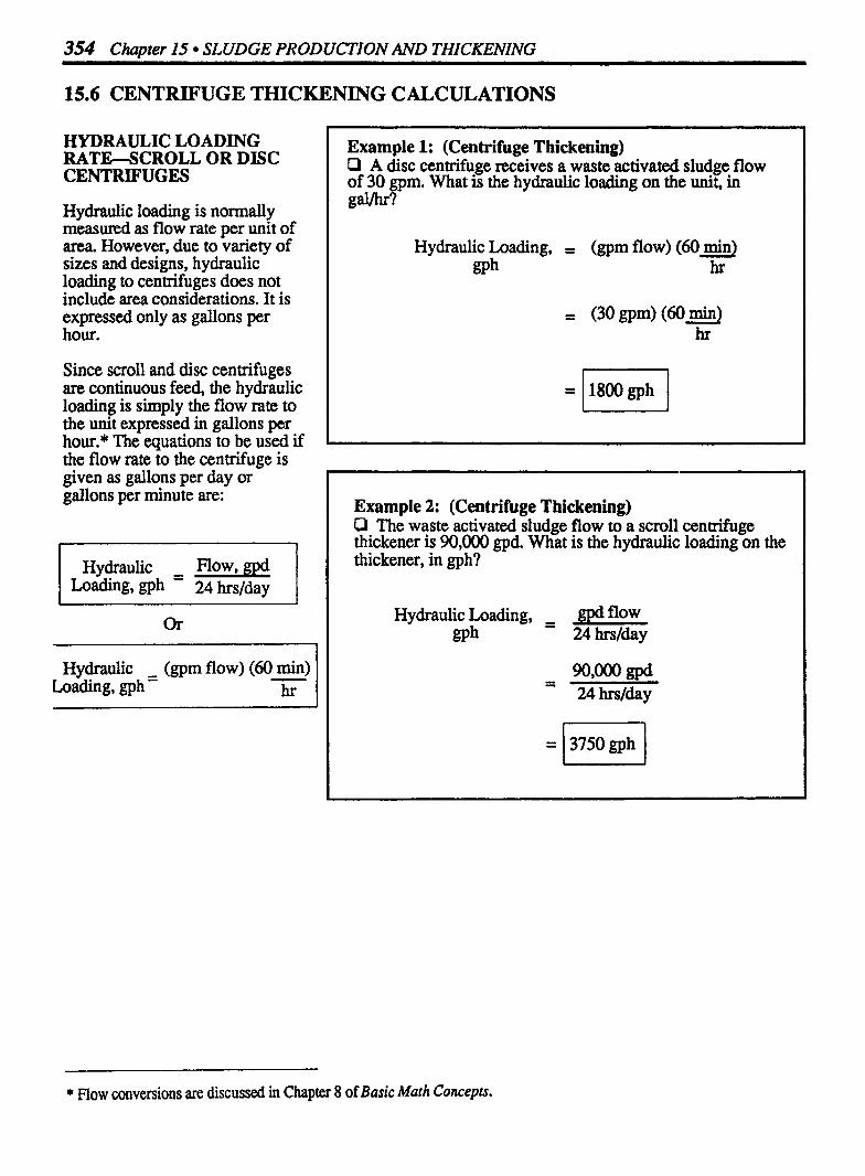
354 Chapter I5 SLUDGE PRODUCTION AND THICKENING
15.6 CENTRIFUGE THICKENING CALCULATIONS
HYDRAULIC LOADING RATE--SCROLL OR DISC CENTRIFUGES
Hydraulic loading is normally measured as flow rate per unit of area However, due to variety of sizes and designs, hydraulic loading to centrifuges does not include area considerations. It is expressed only as gallons per hour.
Since scroll and disc centrifuges are continuous feed, the hydraulic loading is simply the flow rate to the unit expressed in gallons per hour.* The equations to be used if the flow rate to the centrifuge is given as gallons per day or gallons per minute are:
Hydraulic - Flow, gpd Loading, - 24 hrs/day
Hydraulic (gpm flow) (60 min) Loading, gp h ' hr
Example 1: (Centrifuge Thickening) Q A disc centrifuge receives a waste activated sludge flow of 30 gpm. What is the hydraulic loading on the unit, in gal/hr?
Hydraulic Loading, = (gpm flow) (60 min) @h hr
= (30 gpm) (60 min) hr
Example 2: (Centrifuge Thickening) Q The waste activated sludge flow to a scroll ceneifuge thickener is 90,000 gpd. What is the hydraulic loading on the thickener, in gph?
Hydraulic Loading, gpd flow @h - 24 hrs/day
= 1 3750 gph I
* Flow conversions are discussed in Chapter 8 of Basic Moth Concepts.

Centnige Thickening 355
1 1 HYDRAULIC LOADING Example 3: (Centrifbge Thickening) O The waste activated sludge flow to a basket centrifu e is i 60 gpm The basket run time is 25 minutes until the bas et is full of solids. E it takes 142 minutes to skim the solids out of the unit, what is the hydraulic loading on the unit in g m ?
Hydraulic - (gpm) (60 min) (Duration of Sludge Flow, min) Loading, - flow - hr Time in Operation, min
- - (60 gpm) (60 min) (25 min) - hr 26.5 min
RATE--BASKET CENTRIFUGES
Hydraulic loading for basktt cenaifuges is calculated slightly differently than that for scroll or disc centrifuges.
Since scroll or disc centrifuges operate on a continuous feed basis, the hydraulic loading on the unit is simply the flow to the unit expressed as gallons per hour. Basket centrifuges, however, operate on a batch feed basis. Sludge is fed to the unit until the effluent (called centrate) begins to deteriorate. The flow is then stopped and the concentrated sludge is removed from the unit.
Example 4: (Centriluge Thickening) O The sludge flow to a basket centrifb e is 79,000 gpd The fi basket run tune is 22 minutes until the ow to the mt must be stopped for the sldmming operation. If skimming takes 1 - l/2 minutes, what is the hydraulic loading on the unit in gal/hr?
H~dradc - - (gpd flow) (Duration of Sludge Flow, min) Loading' 24 hrs/day Time in Operation, min
mh
- - (79,000 gpd) (22 min) 24 hrslday 23.5 min
During this "down time," therefore, the basket centrifuge is in operation but there is no flow (no hydraulic load) to the unit. You can calculate the hydraulic loading by simply adjusting the flow rate: multiply the flow rate by the fraction of the time sludge was flowing to the unit (the time sludge was fed divided by the total time in operation), as shown below.
Simplified Equation:
(gph) (Duration of ) H Y ~ L flow Sludge Flow
Loading, = Time in Operation
Expanded Equation:
Dur. of Hyd* (am) (60 min) (S1. Flow) Load.,= flow hr Time in-.
gph
Or
1 Dur. of I Hyd. @d flow) (Sl. Flow) Load.,= 24 hrslday Time in Op.
gph
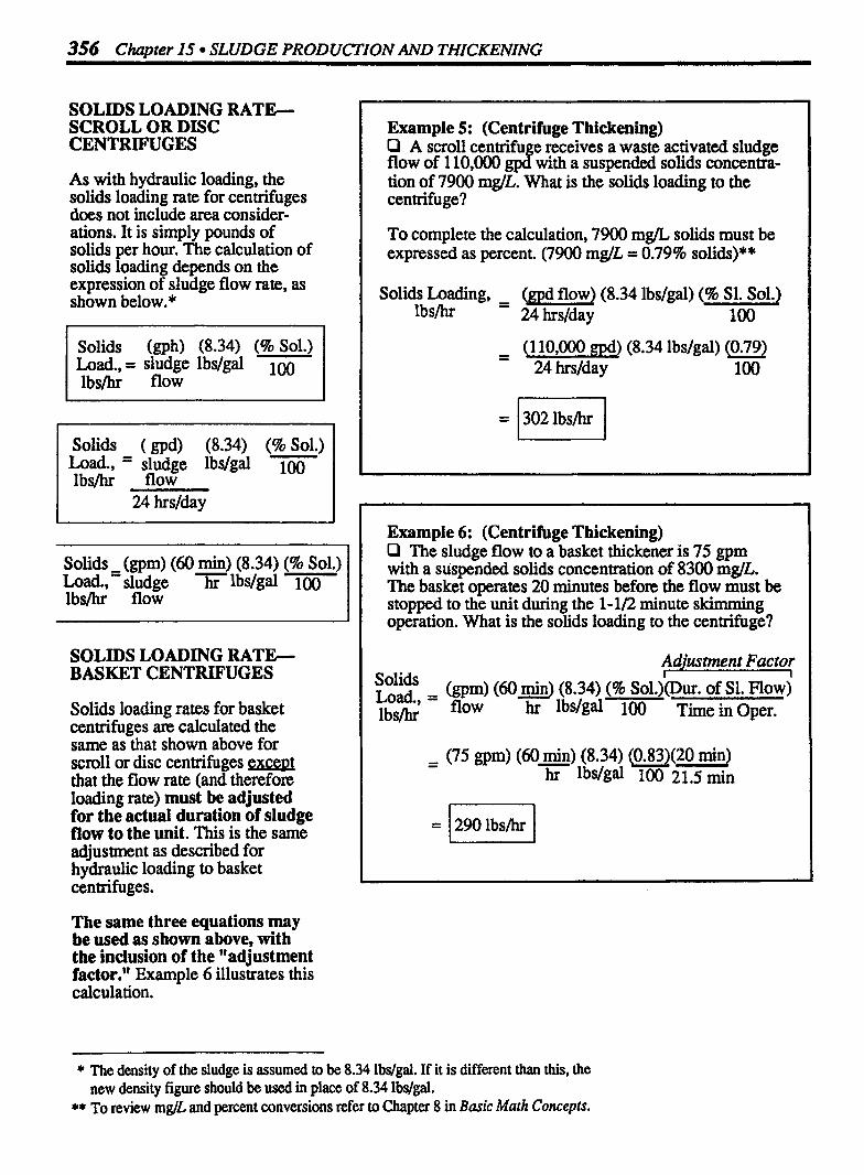
356 Chapter l5 SLUDGE PRODUCFION AND THICKENING
SOLIDS LOADING RATE-- SCROLL OR DISC CENTRIFUGES
As with hydraulic loading, the solids loading rate for centrifuges does not include area consider- ations. It is simply pounds of solids per hour. The calculation of solids loading depends on the expression of sludge flow rate, as shown below.*
Solids (gph) (8.34) (%Sol.) Load., = sludge lbslgal 100 lbs/hr flow
Solids ( a d ) (8.34) (%Sol.) Load., = sludge lbdgal 100 lbs/hr flow
Solids - (gpm) (60 min) (8.34) (% Sol.) Load., - sludge 73- Wgal 100 lbs/hr flow
SOLIDS LOADING RATE--- BASKET CENTRIFUGES
Solids loading rates for basket centrifuges are calculated the same as that shown above for scroll or disc centrifuges g x c a that the flow rate (and therefore loading rate) must be adjusted for the actual duration of sludge flow to the unit. This is the same adjustment as described for hydraulic loading to basket centrifuges.
The same three equations may be used as shown above, with the inclusion of the "adjustment factor." Example 6 illustrates this calculation.
Example 5: (Centrifuge Thickening) O A scroll centrifu e receives a waste activated sludge flow of 110,000 jg.3 with a suspended solids concentra- tion of 7900 mglL. What is the solids loading to the centrifuge?
To complete the calculation, 7900 m@ solids must be expressed as percent. (7900 m& = 0.79% solids)**
Solids Loading, (gpd flow) (8.34 lbslgal) (% Sl. Sol.) lbsjhr
- - 24 hrs/day 100
- - (1 10,000 gpd) (8.34 lbslgal) (0.79) 24 hr slda y 100
Example 6: (Centrifuge Thickening) O The sludge flow to a basket thickener is 75 gprn with a suspended solids concentration of 8300 mglL. The basket operates 20 minutes before the flow must be stopped to the unit during the 1-112 minute skimming operation. What is the solids loading to the ceneifuge?
- - Adjustment Factor
- - (75 gpm) (60 min) (8.34) (0.83)(20 min) hr lbdgal 100 21 .5 min
* The density of the sludge is assumed to be 8.34 lbslgal. If it is different than this, the new density figure should be used in place of 8.34 lbs/gal.
** To review mglL and percent conversions refer to Chapter 8 in Basic Math Concepts.

Centrifuge Thickening 357
Example 7: (Centrifuge Thickening) P A basket centrifuge with a 25 cu ft capacity receives a flow of 65 gprn with a suspended solids concentration of 7800 mg/L.. The average solids concentration within the basket is 7%. What is the feed time for the centrifuge?
(Basket) (7.48) 8.34) (% Bask. Sol.)
cu ft \ Capac., gal/cu ft bs/gal
Fill Time, loo - min - P m) (8.34) (% Inf. Sol.)
ow lbdgal 100
(25 cu ft) (7.48) (8.34) ( 7 ) gal/cu ft lbs/gal 100
= (65 gpm) 8.34) (0.78**) b flow 1 s/gal
Example 8: (Centrifuge Thickening) D A basket centrifuge thickener has a capacity of 16 cu ft. The 55 gprn sludge flow to the thickener has a solids concentration of 8 100 mg/L. The average solids concen- tration within the basket is 9%. What is the feed time for the centrifuge?
(Basket) (7.48) 8.34) (% Bask. Sol.) I Capac., gaVcu ft bslgal FillTime, cu ft 100
- - min (gprn) (8.34) (% Inf. Sol.)
flow lbslgal 100
(16 cu ft) (7.48) (8.34) ( 9 ) gaVcu ft lbslgal 100
(55 gpm) (8.34) (0.8 1) flow lbs/gal 100
FEED TIME (FILL TIME) FOR BASKET CENTRIFUGES
The time required for a batch-fed basket centrifuge to fill with solids depends on several factors:
.The cubic feet volume of the basket,
.The gprn flow to the thickener, and
.The solids concentration of the flow to the thickener.
The feed time (or fill time) calculation is a detention time type of problem. * Simplified Equation:
Expanded Equation:
-
(Bask.) (7.48) (8.34) (% Bask.)
stored sol. Capac., lbs Time, = min Sol. Entering, lbs/min
Fill - Time, - min
cap.; Ibs/gd Solids cu ft cu ft 100
(gprn) (8.34) (% Inf. Sol.) sludge lbslgal 10 flow
Examples 7 and 8 illustrate the calculation of feed time.
* Refer to Chapter 5. ** 7800 mglL is equivalent to 0.78%. For a review of mglL and percent conversions, refer to
Chapter 8, Basic Math Concepts.
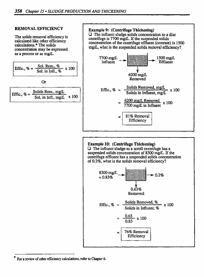
358 Chapter 15 SLUDGE PRODUCTION AND THICKENING
REMOVAL EFFICIENCY
The solids removal efficiency is calculated like other efficiency calculations. * The solids concentration may be expressed as a percent or as mg/L.
Sol. Rem., % Effic., % = Sol. in Infl., %
Solids Rem., mglL Effic., % =
Sol. in Infl., mglL X 100
Example 9: (Centrifuge Thickening) 0 The influent sludge solids concentration to a disc centrifuge is 7700 mglL. If the suspended solids concentration of the centrifuge effluent (centrate) is 1500 mg/L, what is the suspended solids removal efficiency?
6200 mg/L Removed
Effic., % = Solids Removed, mg/L Solids in Influent, mglL
X 100
- - 6200 mgJL Removed 100 7700 mglL in Influent
Efficiency = l 81%
Example 10: (Centrifuge Thickening) Cl The influent sludge to a scroll centrifuge has a suspended solids concentration of 8300 mglL. If the centrifuge effluent has a suspended solids concentration of 0.2%, what is the solids removal efficiency?
Y 0.63%
Removed
Solids Removed, % Effic., % = X 100 Solids in Influent, %
Efficiency = I Removal
* For a review of other efficiency calculations, refer to Chapter 6.
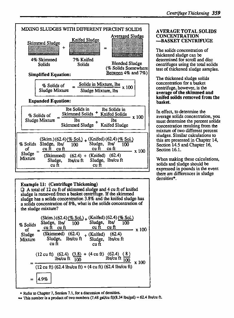
Cenrrifge Thickening 359
MIXING SLUDCES WITH DIFFERENT PERCENT SOLIDS
4% Skimmed Solids
Knifed Sludge
7% Knifed Solids Blended Sludge
(% Solids Somewher Simplified Equation: Between 4% and 7%
% Solids of = Solids in Mixture, lbs Sludge Mixture Sludge Mixture, lbs
Expanded Equation:
I-- lbs Solids in . lbs Solids in % solids of - Skimmed Solids + Knifed Solids
Sludge Mixture lbs + lbs S kifnmed Sludge Knifed Sludge
(Skim.) (62.4) (96 Sol.) + (Knifed) (62.4) (40 Sol.) % Solids Sludge, lbsl 100 Sludge, lbs/ 100
Sludge Mixture (Skimmed) (62.4) + (Knifed) (62.4)
Sludge, lbslcu ft Sludge, lbslcu ft
Example 11: (Centrifuge Thickening) O A total of 12 cu ft of skimmed sludge and 4 cu ft of knifed sludge is removed from a basket centrifuge. If the skimmed sludge has a solids concentration 3.8% and the knifed sludge has a solids concentration of B%, what is the solids concentration of the sludge mixture?
(Skim.) (62.4) (% Sol.) + (Knifed) (62.4) (% Sol.) Sludge lbsl 100 Sludge, lbsl 100 % Solids
cU cu fi of = cu ft cu ft X 100
(12 cu fi) (62.4) (3.8) + (4 cu ft) (62.4) ( 8 ) lbslcu ft 100 lbslcu ft 100
r X loo - -- - - - (12 cu ft) (62.4 ibslcu ft) + (4 cu ft) (62.4 lbslcu ft)
* Refer to Cha~ter 7, Section 7.1, for a discussion of densities.
AVERAGE TOTAL SOLIDS CONCENTRATION -BASKET CENTRIFUGE
The solids concentration of thickened sludge can be determined for scroll and disc centrifuges using the total solids test of thickened sludge samples.
The thickened sludge solids concentration for a basket centrifuge, however, is the average of the skimmed and knifed solids removed from the basket.
In effect, to determine the average solids concentration, you must determine the percent solids concentration resulting from the mixture of two different percent sludges. Similar calculations to this are presented in Chapter 14, Section 14.5 and Chapter 16, Section 16.1.
When making these calculations, solids and sludge should be expressed in pounds in the event there m differences in sludge densities*.
- - - - .
** This numberk a p&uct of t& numbers (7.48 gal/cu ft)(8.34 lbs/gal) = 62.4 lbdcu ft.


1 6 Slucige Digestion
1. Mixing Different Percent Solids Sludges
5% Primary 3% Thickened Blended Sludge Sludge Secondary (96 Solids Somewhere
Sludge &g-3% and 5%) Simplified Equation:
% Solids of = Solids in Mixture, lbdday la) I Sludge Mixture Sludge Mixture, lbslday
( ExpandedEquation:
% Solids of - Prim. Sol., lbslday + Sec. Sol., lbslday sludge Mixture Prim. Sludge, lbslday + Sec. Sludge, lbslday
I 2. Sludge Volume Pumped
Bore
I Simplified Equation:
Volume of Sludge Pumped = (Gallons pumped) (No. of Strokes)
(gavmin) each Stroke each Minute
Expanded Equation: . Volume of
Sludge Pumped = (D2) (Length) (gdmin) Stroke g

362 Chapter l6 SLUDGE DIGESTION
I 3. Sludge Pump Operating Time
I Simplified Equation:
Sludge Removed, lbs/&y = Sludge Pumped, lbs/day
Expanded Equation:
I 4. Volatile Solids to the Digester, Ibslday
r Sludge
If lbs/day solids have already been calculated, either of the following two equations may be used to calculate lbs/day volatile solids:
% Vol. Solids = Vol. Solids, lbs/day Tot. Solids, Ibs/&y
(Tot. Sol.) (96 Vol.) = Vol. Sol. Ibs/&y Solids lbs/day
loo
If lbslday solids have not been determined yet, the following equation can be used to calculate lbs/day volatile solids:
(Sludge) (96) Vol.) - Vol. Sol. lbs/day -- Solids Solids - lbs/day
100 100

I 5. Seed Sludge Based on Digester Capacity
% Seed = Sludge Total Digester Capacity, gal
6. Seed Sludge Based on Volatile Solids Loading
VOLATILE SOLIDS LOADING RATIO COMPARES VS ADDED WITH VS IN THE DIGESTER
lbs/day VS Added 7
Digester lbs VS
Simplified Equation:
Expanded Equation:
(Sludge Added, lbslday ) (% Sol) (% - VS)
VS Loading - - 100 100 Ratio (Sludge in Dig., lbs ) (% Sol) (% VS)
7
100 100
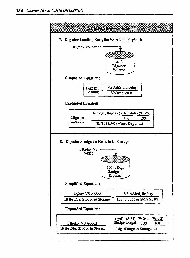
364 Chapter 16 SLUDGE DIGESTION
7. Digester Loading Rate, Ibs VS Added/day/cu ft
lbs/day VS Added -+
Digester
Simplified Equation:
Expanded Equation:
(Sludge, lbs/day ) (% Solids) (% VS) - Digester - - loo loo Loading (0.785) (D2) (Water Depth, ft)
8. Digester Sludge To Remain In Storage
1 lb/day VS Added '-L
10 lbs Dig. Sludge in
Simplified Equation:
I 1 Ib/dw VS Added VS Added, lbslday I - 1 10 lbs Dig. Sludge in Storage Dig. Sludge in Storage, lbs I - P - -
Expanded Equation:
(gpd) (8.34) (% Sol*) (96 VS) p-
1 lb/day VS Added Sludgelbs/gal 100 100 - 10 lbs Dig. Sludge in Storage Dig. Sludge in Storage, lbs

9. Volatile AciddAlkalinity Ratio
Volatile Acids/Alkalinity - - Volatile Acids, m@L Ratio Alkalinity, mg/L
10. Lime Required for Neutralization
Volatile Acids = Lime Required lbs lbs
(mgt") Pig. Vol.) (8.34) - Ibs Volatile Volatile MG W g d - Acids
Acids - - lbs Lime
Required
I 11. Percent Volatile Solids Reduction
When Volatile Solids Are Expressed as Pounds:
% VS = VS Reduced, lbs Reduction Total VS Entering, lbs
When Volatile Solids Are Expressed As Percents:
There are two equations that may be used to calculate percent volatile solids reduction.
% vs = (% VS In - % VS Out) X 100
Reduction % VS - (% VS) (% VS ) In In Out
In the equation shown below, the "In" and "Out" data are written as decimal fractions.
% vs = Reduction In - (In X Out) In - Out loo l

366 Chapter 16 SLUDGE DIGESTION
12. Volatile Solids Destroyed, lbs VSIdaylcu ft
lbs/day VS Reduction
Digester U I cu ft Volume
I Simplified Equation:
VS Destroyed, lbs/day Destroyed, =
lbs VS/day/cu ft Dig* Volume, cu ft
I Expanded Equation:
(gpd) (8.34) (% Sol.) (% VS)(% VS Red.) p-
Volatile Solids Sludge lbs/gal 100 100 100 Destroyed, =
lbs VS/day/cu ft (0.785)(D2)(depth, ft)
I 13. Digester Gas Production
Simplified Equation:
Expanded Equation:
1 Digester Gas Gas Produced, cu ft/day I I Pioduction (Vol. Sol. to Dig.) (% VS Reduction )
lbslday 100 I

14. Digester Solids Balance SOLIDS BALANCE FOR DIGESTER
'WHAT GOES IN, MUST COME OUT"
SLUDGE IN = SLUDGE OUT + GAS + H20
v Total Solids
Total Solids + Water = Total Solids +Water + Gas rl-1 rl-l
Vol. Solids Fixed Solids Vol. Solids Fixed Solids
Calculations 1-14 are applicable to anaerobic a aerobic digestion. (Calculation 13 is a calculation used for anaerobic digestion.) Calculations 15- 17 apply particularly to aerobic dieestion.
l
15. Digestion Time
Digester a d -kume J-
Sludge gallons Flow
I Simplified Equation:
Digestion - Digester Volume, gal Time, - Sludge Flow Rate, gpd
l Expanded Equation:
Digestion - - (0.785)@ )(depth, ft)(7.48 gdcu ft) Time, days Sludge Flow Rate, gpd

368 Chapter 16 SLUDGE DIGESTION
16. Air Requirements and Oxygen Uptake
Air Requirements:
Simdified Eauation;
0.02 cfm Air - Air Req., cfm 1 cu ft Dig. Vol Dig. Vol., cu ft
For circular digesters
0.02 cfm Air - I 1 cu ft - (0.785)(D2)(depth, ft)
I For rectangular digesters
Oxygen Uptake:
sim~lified Eauation;
mglL DO used 0 2 Uptake, - during Test 60 min -
mg/L/hr Min. during hr Measurement
Expanded Eauation;
I min min I
17. pH Adjustment Using Jar Tests
(mg/L) (MG) (8.34) = lbs Lime Lme or Dig- lbslgal or Caustic Caustic Vol.

370 Chapter l6 SLUDGE DIGESTION
16.1 MIXING DIFFERENT PERCENT SOLIDS SLUDGES
When sludges with different percent solids content are mixed, the resulting sludge has a percent solids content somewhe~ between the solids contents of the original sludges. For example, if a primary sludge with a 4% solids content were mixed with a secondary sludge with a 1% solids content, the resulting sludge might have a solids content of about 2 or 3%. The actual percent solids content will depend on how much (lbs) of each sludge is mixed together. If, in the example, most of the sludge was from the secondary sludge (1 % solids) and very little&-om the primary sludge (4% solids), then the resulting sludge would be closer to a 1 % sludge- perhaps a 1 .5 % sludge. If, on the other hand, most of the sludge was primary sludge and very little was secondary sludge, then the resulting sludge mixture might have a solids content closer to 4%-such as 3 or 3.5%.
The actual solids content of a mixture of two or more sludges depends on:
the pounds of sludge contributed from each source, and
the percent solids of each sludge.
As with the sludge thickening equation, remember that if the thickened sludge has a density different than 8.34 lbslgal, it should be used in the equation instead of 8.34 lbs/gal.*
WHEN SLUDGES ARE MIXED, THE MKXTURE HAS A % SOLIDS CONTENT BETWEEN THE TWO
ORIGINAL % SOLIDS VALUES
Rimary Sludge with Thickened Blended
5% Solids Secondary Sludge Sludge with (% Solids Somewhere 3% Solids ~etween 3% and 5%)
Simplified Equation:
% Solids of = Solids in Mixture, lbslday sludge Mixture Sludge Mixture, lbs/day
Expanded Equation:
%Solidsof Prim.Sol.,lbs/day+Sec.Sol.,lbs/day xlOO - Sludge - Prim. Sludge + Sec. Sludge Mixture lbslday lbslday
Example 1: (Mixing Sludges ) P A rimary slud e (5% solids) flow of 7540 gpd is mixed with a thicf:ened secon& sludge (3% solids) flow of 3220 gpd. What is the percent solids content of the mixed sludge flow?
% of Rim. SL sol., lbs/day + Sec. SI. sol., lbs/day 100 Sludge = Mixtwe Prim. Sludge, lbslday + Sec. Sludge, lbslday
(7540 gpd) (8.34) ( 5 ) + (3220 gpd) (8.34) ( 3 ) - - Prim. S1. lbslgal 1 0 Sec. S1. lbslgal 100
X 100 - - - - - (7540 gpd) (8.34) + (3220 gpd) (8.34)
Prim. lbslgal Sec. lbslgal Sludge Sludge
- - 3144lbsldayPrim Sol + 8061bs/&y Sec. Sol. 100
62,884 lbslday + 26,855 lbsjday
- - 3950 lbslday Solids 89,7 39 lbslday Sludge
* Refer to Chapter 7, Section 7.1, for a review of density and specific gravity.

Mixing Sludges 371
Example 2: (Mixing Sludges ) 0 Primary and thickened secondary sludges are to be mixed and sent to the digester. The 5930 gpd primary sludge has a solids content of 4.846; the 2660 gpd thickened secondary sludge has a solids content of 3.8%.What would be the percent solids content of the mixed sludge?
95 Solids of Prim. Sol., lbslday + Sec. Sol., lbslda X 100
'ludge = Prim. Sludge, lbslday + Sec. Sludge, lklday Mixture
(5930 gpd) (8.34) ( 4.8 + (2660 gpd) (8.34) ( 3.8 ) - Prim. S1. lbslgal 100 - Sec. S1. lbslgal 100
X 1 0 -- - - v
(5930 gpd) (8.34) + (2660 gpd) (8.34) Prim. lbslgal Sec. lbdgal Sludge Sludge
- - 2374 lbslday + 843 1bs 100 49,456 lbslday + 22,184
- - 3217 lbsfday Solids 100 7 1,640 lbslday
= 1 4.5% Solids l
Example 3: (Mixing Sludges ) Q A primary sludge flow (3.8% solids) of 6720 is mixed with a thickened secondary sludge flow (5% soli p ) of 3670 gpd. What is the percent solids of the combined sludge flow?
% solids of lbslday Prim. Sol. + lbslday Sec. Sol. X 100
' lbsfday Prim. Sludge + lbslday Sec. Sludge Mixture
(6720 gpd) (8.34) (3.8 ) + (3670) (8.34) ( 5 ) - - Prim. S1. lbslgal 100 Sec. S1. lbslgal 100 ,
(6720 gpd) (8.34 lbs/gal) + (3670) (8.34 lbslgal)
- 2130 lbs/day + 1530 lbslday 56,045 lbslday + 30,608 lbslday
- - 3660 lbslday Solids 86,653 lbslday Sludge
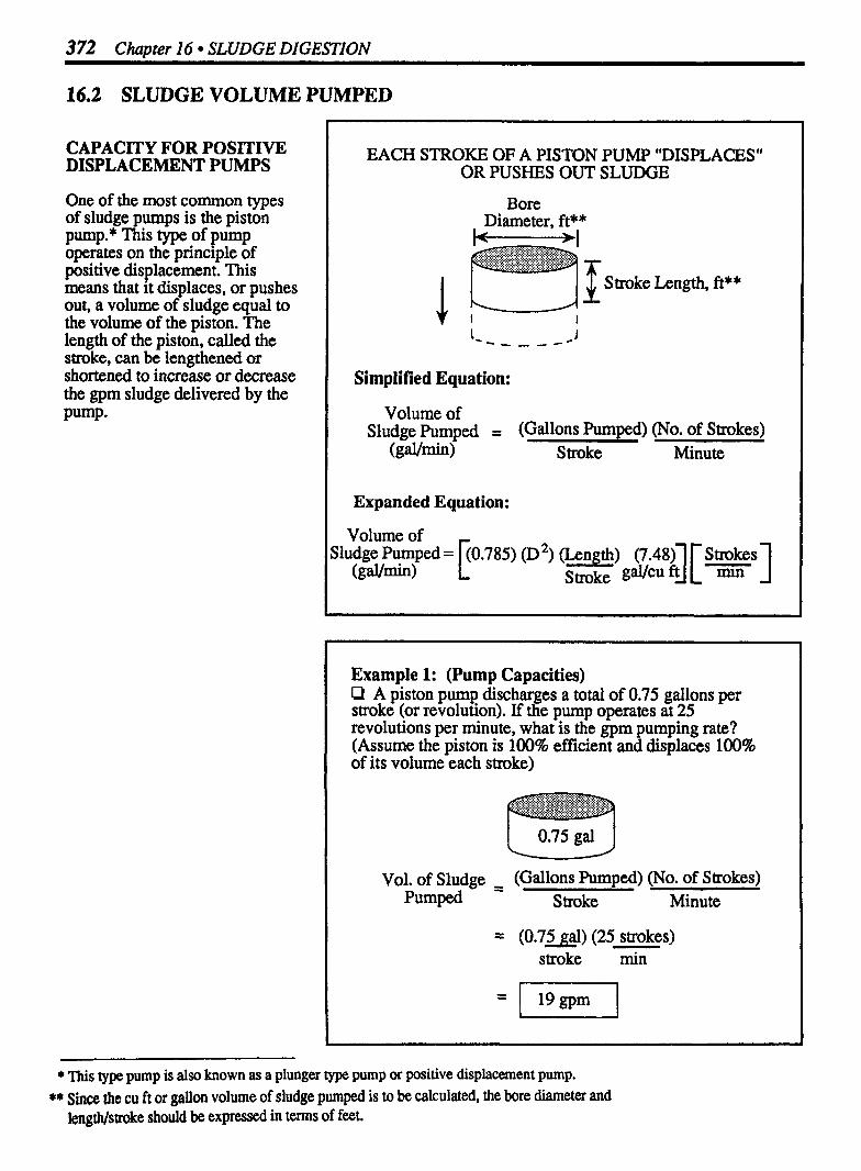
372 Chapter 16 SLUDGE DIGESTION
16.2 SLUDGE VOLUME PUMPED
CAPACITY FOR POSITIVE DISPLACEMENT PUMPS
One of the most common types of sludge pumps is the piston pump.* This type of pump operates on the principle of positive displacement. This means that it displaces, or pushes out, a volume of sludge equal to the volume of the piston. The length of the piston, called the stroke, can be lengthened or shortened to increase or decrease the gpm sludge delivered by the Pump-
EACH STROKE OF A PISTON PUMP "DISPLACES" OR PUSHES OUT SLUDGE
Bore
1 Stroke Length, ft**
Simplified Equation:
Volume of Sludge Pumped = (Gallons Pumped) (No. of Strokes)
Expanded Equation:
Volume of Sludge Pumped = p.785) (D2) (Length) (7.48)] [~trokes]
(gal/&) -
Stroke gdcuft m
Example 1: (Pump Capacities) Q A piston pump discharges a total of 0.75 gallons per stroke (or revolution). If the pump operates at 25 revolutions per minute, what is the gpm pumping rate? (Assume the piston is 100% efficient and displaces 100% of its volume each stroke)
Vol. of Sludge - - (Gallons Pumped) (No. of Strokes) Pumped Stroke Minute
= (0.75 gal) (25 strokes) stroke min
* This type pump is also known as a plunger type pump or positive displacement pump.
** Since the cu ft or gallon volume of sludge pumped is to be calculated, the bore diameter and IengthJstroke should be expressed in terms of feet.

Sludge Volume Pumped 373
Example 2: (Pump Capacities) P A sludge pump has abore of 10 inches and a stroke of 4 inches. If the pump operates at 35 strokes (or revolutions) per minute, how many gprn are pumped? (Assume the piston is 100% efficient and displaces 100% of its volume each stroke.)
Vol. of Sludge - - (Gallons Pumped) (No. of Strokes) Pumped Stroke Minute
= Stroke g
(0.83 ft) (0.83 ft) (0.33 ft) (7.48 Stroke
- - (1.33 gal) (35 Strokes) Stroke min
Example 3: (Pump Capacities) P A sludge ump has a bore of 8 inches and a stroke setting of 3 inches. h e pump operates at 50 revolutions per minute. If the pump operates a total of 90 minutes during a 24-hour period, what is the gpd pumping rate? (Assume the piston is 100% efficient.)
First calculate the gpm pumping rate: Vol. Pumped = (Gallons Pumped) (No. of Strokes)
Stroke Minute
(0.67 ft) (0.67 ft)
= (0.66 gal) (50 strokes) stroke min
= 33 gprn Then convert gprn to gpd pumping rate, based on total minutes pumped during 24-hours:
(33 gpm) (90 - min) =
day
CALCULATING GPD PUMPED
There are two methods to determine gpd pumping rate:
Calculate the gpm pumping rate, then multiply by the total minutes operation during the 24-hour period:
Pumping = (Pumping) (Total min) Rate, Rate, gprn pumping gpd in 24 hrs
Calculate the gallons pumped each revolution, then multiply by the total revolutions during the 24-hour period:
l Pumping = (Gallons) (Total Revol.) Ra% Revolution day I

374 Chiwter 16 SLUDGE DIGESTION
16.3 SLUDGE PUMP OPERATING TIME
The sludge pump operating time depends on the amount of sludge to be removed. As shown to the right, the basis of this calculation is simply-the lwday sludge to be removed is set equal to the lbs/day sludge to be pumped. Examples 1-3 illustrate this calculation.
REQUIRED SLUDGE PUMPING RATE DEPENDS ON SLUDGE REMOVED PER DAY
Simplified Equation:
I Sludge Removed, lbs/day = Sludge Pumped, lbs/day I Expanded Equation:
(mglL) (MGD) (8.34) SS Rem. flow lbs/gal
% Solids 100
(W@ (xmin) Sludge
Pumping day Rate -
Example 1: (Sludge Pump Operating Time) O The flow to a primary clarifier is 2 MGD. The influent suspended solids concentration is 210 mglL and the effluent suspended solids concentration is 108 mglL. If the sludge to be removed from the clarifier has a solids content of 3.5% and the sludge pumping rate is 30 gpm, how many minutes per hour should the pump operate?
First calculate min/day pumping rate ~quired:
Sludge Removed, lbs/&y = Sludge Pumped, lbs/day
(m@) (MGD) (8.34) (@m) (X min) (8.34) SS Rem. flow lbdgal - Sludge &y lbs/gal
% Solids - Pumping 100 Rate
194 rnin/day = X
Then convert minjday to min/hr:
* For a review of calculating lbs/day sludge to be removed (the left side of the equation), refer to Chapter 15, Section 15.2.

Sl@e Pump Operating Time 375
Example 2: (Sludge Pump Operating Time) O A primary c ld i e r receives a flow of 3,600,000 gpd with a suspended solids concentration of 225 mglL. The clarifier effluent has a suspended solids concentration of 95 mglL. If the sludge to be removed from the clarifier has a solids content of 4% and the sludge pumping rate is 45 gpm, how many minutes per hour should the pump operate?
First calculate min/day pumping rate required:
Sludge Removed, lbslday = Sludge Pumped, lbslday
Then convert midday to min/hr:
Example 3: (Sludge Pump Operating Time) Cl The flow to a primary clarifier is 1.7 MGD, with a suspended solids concentration of 205 mglL. The clarifier effluent suspended solids concentration is 90 mgIL. The sludge to be removed fiom the clarifier has a solids content of 3%. If the sludge pumping rate is 30 gpm, how many minutes per hour should the pump operate?
First determine the min/day pumping rate required:
Sludge Removed, lbs/day = Sludge Pumped, lbslday
(115 mg,L)(1.7 MGD) (8.34) lbskal - - (30 gpm)(x min) (8.34)
0.03 G lbslgal
Then convert min/day to min/hr:

376 Chapter 16 SLUDGE DIGESTON
16.4 VOLATILE SOLIDS TO THE DIGESTER
Sludge solids are comprised of organic matter (from plant or animal sources) and inorganic matter (material from mineral sources, such as sand and grit). The organic matter is called volatile solids, and the inorganic matter is called fixed solids. Together, the volatile solids and fixed solids make up the total solids.
When calculating percent volatile solids, it is essential to remember the general concept of percent:
Part Percent = -
Whole X100 /
When calculating percent vola- tile solids, the "part" of interest is the weight of thk volatile solids; the "whole" is the weight of total solids:
% Vol. - Vol. Sol., lbslday , "lids - Tot. Sol., lbslday
To calculate lbslday volatile solids to the digester, this equation is often rearranged as:
(Tot. Sol.) (% Vol. Sol.) - - vol. sol. lbslday 100 l b sjday
COMPARING % SOLIDS AND % VOLATILE SOLIDS CALCULATIONS
% Solids
Sludge
Using lab data:
Solids, grams Solids Sludge, grams
Using plant data:
% = Solids. lbs ,100 Solids Sludge, lbs
Or (Rearranged as)
(Sludge, lbs) (% Solids) = Solids 100 lbs
% Volatile Solids
Total Solids - Fixed Solids - Volatile
Solids
Using lab data: pp
Solids Tot. Sol., g
Using plant data:
% 0 . = Vol. Sol*, lbslda~ ,, I Solids Tot. Sol., lbs/day
Or (Rearrangedas)
(Tot. Sol.) (% Vol.) Vol. Sol* lbslday Sol. = lbsjday
100
Example 1: (% Volatile Solids) Q If 1480 lbslday solids are sent to the di ester, with a
solids are sent to the digester? f volatile solids content of 70%, how many bslday volatile
Write the equation, then fill in the known information:
(Total Solids) (% Vol. Solids) = Vol. Solids l bslday 100 l b slday
(1480 lbslday) ( 100 Vol. Solids
* The calculation of volatile solids using laboratory data described in greater detail in Chapter 18.

Volatile Solidr to the Digester 377
Example 2: (% Volatile Solids) O A total of 3240 gpd sludge is to be pumped to the digester. If the sludge has a 5% solids content with 68% volatile solids, how many lbs/day volatile solids are pumped to the digester?
(Sludge) (% Solids) (%Vol. Sol.) = Vol. Sol. Wday 1 0 100 lbs/day
Since sludge is given in gpd, it must be multiplied by 8.34 lbs/gal to convert gpd sludge to lbs/day sludge:*
lbslday Sludge I l
Vol. Sol. (% Vol. Sol.) = lbs/day loo
(3240) (8.34) (0.05) (0.68) = gpd lbs/gal Vol. Sol.
Example 3: (% Volatile Solids) P A total of 5480 gpd sludge is to be pumped to the digester. If the sludge has a total solids content of 4.5% and a volatile solids content of 72%, how many lbs/&y volatile solids are pumped to the digester? (Assume thc sludge weighs 8.34 lbs/gal.)**
lbs/&y Sludge - ?sludge) (8.343 (% Solids) (% Vol. Sol.) = Vol. Sol.
gpdlbskal 100 100 lbs/&y
(5480) (8.34 (0.045) (0.72) = ( 1481 lbs/&y ( gpd lbs/g a vol. Sol.
CALCULATING VOLATILE SOLIDS GIVEN SLUDGE DATA
Sometimes you will have lbs/day sludge information and will want to calculate lbs/day volatile solids. When this is the case, you must include the percent solids factor in the equation as well, shown in the equation below. In effect, you are calculating lbs/day solids fmt, (using the percent solids factor), then the lbs/day volatile solids (using the % volatile solids factor):
(Sludge) (%) (96 Vol.) lbs/&y Soh& Solids = --
loo loo
* For a review of flow conversions, refer to Chapter 8 in Baric Math Concepts. * * Remember, if the sludge has a density greater than than of water, a factor greater than 8.34 lbs/gal
must be used. Refer to Chapter 7 for a discussion of density and specific gravity.

378 Chapter 16 SLUDGE DIGESTION
16.5 SEED SLUDGE BASED ON DIGESTER CAPACITY
There are many methods to determine seed sludge required to start a new digester. One method is to calculate seed sludge required based on the volume of the digester. Examples 1-4 illustrate this calculation.
Most digesters have cone-shaped bottoms. For simplicity, however, the side water depth ( S W ) is commonly used to represent the average digester depth.
Although determining seed sludge requirements based on digester volume can give you a quick estimate of seed sludge required, it is not sensitive to the balance between the volatile solids in the seed sludge and the volatile solids in the incoming sludge. A calculation of seed sludge requirements based on volatile solids loading is given in the next section.
Example 1: (9% Seed Sludge) Q A digester has a capacity of 250,000 allons. If the digester seed sludge is to be 25% of the %I 'gester capacity, how many gallons of seed sludge will be required?*
_I gallons 25% 1
% Seed - Seed Sludge, gal - Total Digester Capacity, gal X loo
X gal Seed Sludge 25 = 250,000 gal Capacity
(250,000 gal) ( 25 ) = X
100
Example 2: (96 Seed Sludge) Q A 50-ft diameter digester has a t ical water depth of 20 ft. If the seed sludge to be used is 2 & o of the tank capacity, how many gallons of seed sludge will be required?*
% Seed = Seed Sludge, gal Sludge Total Digester Capacity, gal
20 = X gal Seed Sludge
X loo (0.785) (50 ft) (50 ft) (20 ft) (7.48 gaVcu ft)
(0.785) (50 ft) (SO ft) (20 ft) (7.48) (20) = X
100
* For a review of volume calculations, refer to Chapter 11 in Basic Math Concepts.

Seed Sludge Based on Digester Capacity 379
Example 3: (% Seed Sludge) P A digester 40 ft in diameter has a side water depth of 20 ft. If the digester seed sludge is to be 22% of the digester capacity, how many gallons of seed sludge will be required?
% Seed - , Seed Sludge, gal X 100 Sludge Total Digester Capacity, gal
x gal Seed Sludge 22 = X 100
(0.785) (40 ft) (40 ft) (20 ft) (7.48 gaVcu ft)
(0.785) (40 ft) (40 ft) (20 ft) (7.48) (22) = X
100
1 41,337gd 1 = X Seed Sludge
Example 4: (% Seed Sludge) Ll A 40-ft diameter digester has a typical side water depth of 18 ft. If 52,100 gallons seed sludge are to be used in starting up the digester what percent of the digester volume will be seed sludge?
% Seed , Seed Sluage, gal X 100 Sludge Total Digester Capacity, gal
X = 52,100 gal Seed Sludge
X 100 (0.785) (40 ft) (40 ft) (18 ft) (7.48 gaVcu ft)
CALCULATING OTHER UNKNOWN FACTORS
There are three variables in percent seed sludge calcula- tions: percent seed sludge, gallons seed sludge, and total gallons digester capacity.
In Examples 1-3, the unknown factor was seed sludge gallons. However, the same equation can be used to calculate either one of the other two variables. In Example 4 the variable is percent seed sludge.

380 Chapter 16 SLUDGE DIGESTION
16.6 SEED SLUDGE BASED ON VOLATILE SOLIDS LOADING
One way of calculating seed sludge requirements was dcscribtd in the previous section-seed sludge based on a percent of the digester volume. Another way to express digester loading is based on lbs/day volatile solids* added daily per each lb of volatile solids under digestion (in the digesters).
VOLATILE SOLIDS LOADING RATIO COMPARES VS ADDED DAILY WITH VS IN THE DIGESTER
VS Added 1
Digester I lbs VS
Simplified Equation: U
VS Loading - VS Added, Wday Ratio VS in Digester, lbs
Expanded Equation:
(Sludge Added, lbs/day ) (% Sol) (% VS) v-
VS Loading - - 100 100 Ratio (Sludge in Dig., lbs ) (% Sol) (% VS)
p-
loo 100
Example 1: (Volatile Solids Loading Ratio) P A total of 64,900 lbs/day slud e is pumped to a 100,000-gallon digester. The slu f ge being pumped to the digester has total solids content of 5.5% and volatile solids content of 67%. The sludge in the digester has a solids content of 6% with a 56% volatile solids content. What is the volatile solids loading on the digester in lbs VS added/day/lb VS in digester?
VS Loading - - VS Added, Wday Ratio VS in Digester, lbs
loo loo - - - -
, ( l ~ , o o O gal) (8.34 1bdga.l) ( 6 ) ( 56 ) I- -
I 'loo 100 This is lbs digester sludge
* For a review of calculating percent solids and percent volatile solids, refer to Chapters 6 (Section 6.4) and Chapter 18 (Section 18.6).
= 0.0851bs VS Addeaday lbs VS in Digester

Seed Sludge Based on VS Louding 381
Example 2: (Volatile Solids Loading Ratio) P A total of 20,700 gal of digested slud e is in a di ester. The digested sludge contains 6% total so % 'ds and 58 k volatile solids. If the desired VS loading ratio is 0.05 lbs VS added/day/lb VS under digestion, what is the & s k i lbs VS/day to enter the digester?
0.05 = x lbs VS A d d d a y
I (20,700 gal) (8.34 lbs/gal), ( 6 ) ( 58 ) --
L
This is lbs digester sludge 'loo 100
Now solve for the unknown value:*
Example 3: (Volatile Solids Loading Ratio) O A new di ester 50 ft in diameter is o rating at an average B depth of 25 t. The raw sludge flow to 8 e digester is expected to be 820 gpd. The raw sludge contains 6% solids and 72% volatile solids. ?he desired VS loading ratio is 0.07 lbs VSlday/lb VS in digester. How many gallons of seed sludge will be required if the seed sludge contains 9% solids with a 52% volatile solids content? (Assume the seed sludge weighs 9 lbs/gal.)
(Sludge Added, lbslday ) (% Sol) (% VS) VS Loading - - 100 100
Ratio (Seed Sludge in Dig., lbs S) (96 Sol) (% VS) 100 100
This is lbslday sludge added I
0.07 = (820 gpd) (8.34 1bslgal)'(0.06) (0.72)
I (X gal seed) (9 lbslgal) ,(0.09) (0.52) This is lbs seed sludge
Now solve for X*:
= 1 10,020 gal Seed sludgel
CALCULATING OTHER UNKNOWN VALUES
Volatile solids loading ratio calculations have three variables: VS loading ratio, lbs VS added daily, and lbs VS in the digester.
Given a desired VS loading ratio, you can calculate either of the other two variables, as shown in Examples 2 and 3.
* Refer to Chapter 2 in Basic Math Concepts for a review of solving for the unknown value.

382 Chapter 16 SLUDGE DIGESTION
16.7 DIGESTER LOADING RATE, Ibs VS Addedldaylcu ft
Sludge is sent to a digester in order to break down or stabilize the organic portion of the sludge. Therefore, it is the organic part of the sludge (the volatile solids) that are of interest when calcu- lating solids loading on a digester.
Digester loading rate is a measure of the lbs volatile solids/day* entering each cubic foot of digester volume, as illustrated in the diagram to the right.
DIGESTER LOADING RATE
VS Added -1
Digester Volume
L C U f t J Simplified Equation:
Expanded Equation:
(Sludge. l b s h Die Loaamg (0.785) (D2) (Water Depth, ft)
Example 1: (Digester Loading Rate) Cl A digester 40 ft in diameter with a water depth of 20 ft receives 84,000 lbs/day raw sludge. If the sludge contains 6.5% solids with 70% volatile matter, what is the digester loading in lbs VS addeaday /cu ft volume?
VS Added lbsldav '-&
(Sludge, lbs/day ) (% Solids) (% VS) Digester = 100 100 Loading (0.785) (D2) (Water Depth, ft)
- (84,000 lbs/day) (0.065) (0.70) (0.7 85) (40 ft) (40 ft) (20 ft)
= 1 0.15 lbs VS/day cu ft
* For a review of calculating percent solids and percent volatile solids, refer to Chapters 6 (Section 6.4) and Chapter 18, Section 18.6.

Digester Loading Rate 383
Example 2: (Digester Loading Rate) Cl A digester 50 ft in diameter with a liquid level of 20 ft receives 36,900 gpd sludge with 5.5% solids and 70% volatile solids. What is the digester loading in lbs VS addedlday /cu ft volume?
VS Added l b s/day
Digester cu ft Volume
(gpd sludge) (8.34 lbslgal) (% Sol) (% VS) Digester - - -. - 100 100 Loading - (0.785) (D2) (Water Depth, ft)
(36,900 gpd) (8.34 lbslgal) (0.055) (0.70) (0.785) (50 ft) (50 ft) (20 ft)
= I 0.30 lbs VS/day I cu ft
Example 3: (Digester Loading Rate) C1 A digester 40 ft in diameter with a li uid level of 18 ft receives 175,000 lbslday sludge with 5 9 o total solids and 72% volatile solids. What is the digester loading in lbs VS added/day per 1000 cu ft?
. :: .:.:.:.:.:.*.:::.:.:.:.:.:.: ...... . . ..>: :::k;;:;;~~~;:$>i<~i:3#:~.~: .,.. ....................................... ................................... volume . ....... . ..................... ... . . . . . . . . . . ........... ...:z.....'.'... ...... (0.785) (40 ft) (40 ft) (18 ft) = 22,608 cu ft
Volume = 22.6 Thousand cu ft
(lbslday Sludge) (% Solids) (% VS) Digester = 100 100 Loading (0.785) @2) (Water Depth, ft)
= 1 279 lbs VSIday 1 1000-cu ft
GIVEN GPD OR GPM SLUDGE PUMPED TO DIGESTER
In Example 1, sludge pumped to the digester was expressed as lbslday . Most times, however, sludge pumped to the digester will be expressed as gpd or gpm. When this is the case, convert the gpd or gpm pumping rate to lbslday* and continue as in Example 1. You can make the gpd to lbslday conversion a separate calculation, or you can incorporate it into the numerator of the equation as shown in Example 2.
DIGESTER LOADING RATE AS LBIDAY VS/1000 CU FT
Digester loading is sometimes expressed as lbs volatile solids added/day per 1 OOO cu ft digester volume:
Digester - VS Added, lbslday Loading - Volume, 1000-cu ft
When this is the case, express the cu ft volume as 1000 cu ft before using it in the denominator. For example, if the digester volume were 35,000 cu ft, then you would use 35 in the denominator of the equation. Remember that the " 1000", as part of the "1000-cu ft" in the denominator, is a unit of measure and is not part of the calculation. Example 3 illustrates this calculation.
* To review flow conversions, refer to Chapter 8 in Basic Math Concepts.
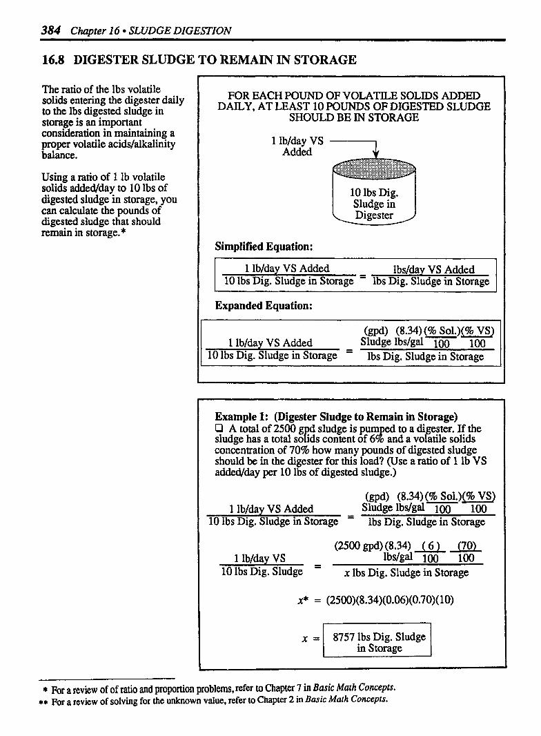
384 Chapter 16 SLUDGE DIGESTION
16.8 DIGESTER SLUDGE TO REMAIN IN STORAGE
The ratio of the lbs volatile solids entering the digester daily to the lbs digested sludge in storage is an important consideration in maintaining a proper volatile acids/alkalinity balance.
Using a ratio of 1 lb volatile solids added/day to 10 lbs of digested sludge in storage, you can calculate the pounds of digested sludge that should remain in storage.*
FOR EACH POUND OF VOLATILE SOLIDS ADDED DAILY, AT LEAST 10 POUNDS OF DIGESTED SLUDGE
SHOULD BE IN STORAGE
1 lb/day VS Added --l
10 lbs Dig. Sludge in
Simplified Equation:
1 lblday VS Added - lbslday VS Added 10 lbs Dig. Sludge in Storage - lbs Dig. Sludge in Storage
Expanded Equation:
(gpd) (8.34) (% Sol.)(% VS) 1 lb/day VS Added - Sludge l b s l g a l ~ 100
10 lbs Dig. Sludge in Storage - lbs Dig. Sludge in Storage
Example 1: (Digester Sludge to Remain in Storage) Q A total of 2500 sludge is pum ed to a digester. If the ppd sludge has a total so ids content of 6 ?if' o and a volatile solids concentration of 70% how many pounds of digested sludge should be in the digester for this load? (Use a ratio of 1 lb VS added/day per 10 lbs of digested sludge.)
(gpd) (8.34) (% Sol.)(% VS) 1 lb/day VS Added - Sludge lbs/gal-i@- 1 0
l0 lbs Dig. Sludge in Storage - lbs Dig. Sludge in Storage
(2500 gpd) (8.34) ( 6 ) (70) 1 lb/day VS - 100 100
10 lbs Dig. Sludge - x lbs Dig. Sludge in Storage
X = ( 8757 lbs Dig. Sludge in S torage
* For a review of of ratio and proportion problems, refer to Chapter 7 in Basic Math Concepts. ** For a review of solving for the unknown value, refer to Chapter 2 in Basic Math Concepts.

Digester Sludge to Remain in Storage 385
Example 2: (Digester Sludge to Remain in Storage) Q A total of 5000 gpd sludge is pum d to a digester. The sludge has a solids concentration of 8% and a volatile solids content of 67%. How many pounds of digested sludge should be in the digester for this load? (Use the ratio of 1 lb VS addeaday per 10 lbs digested sludge.)
(gpd) (8.34) (% Sol.)(% VS) 1 lblday VS Added Sludge l b s l g a l ~ 100
10 lbs Dig. Sludge in Storage - lbs Dig. Sludge in Storage
-- p
10 lbs Dig. Sludge -
x lbs Dig. Sludge in Storage
= I 1 8,160 lbs Digested Sludge 1
Example 3: (Digester Sludge to Remain in Storage) Cl A digester receives a flow of 3000 allons of sludge during a 24-hour period. If the sludge as a solids content of 7% solids and a volatile solids concentration of 72%, how many pounds of digested sludge should be in the digester for this load? (Use the ratio of 1 lb VS addeaday per 10 lbs digested sludge.)
(gpd) (8.34) (% Sol.)(% VS) l lblday VS Added - Sludge l b s l g a l ~ 10
10 lbs Dig. Sludge in Storage -
lbs Dig. Sludge in Storage
- 10 lbs Dig. Sludge X lbs Dig. Sludge in Storage
= 1 12,610 lbs Digested Sludge /

386 Chapter 16 SLUDGE DIGESTION
16.9 VOLATILE ACIDSIALKALINITY RATIO
The process of anaerobic digestion occurs in two basic stages, both of which are in intricate balance. The first phase of digestion is that of acid fermentation and is related to the fmt stage in the digestion of new volatile solids entering the digester. The second stage of digestion, methane fermentation, occurs in a more alkaline environment and is thus indicative of advanced stages of digestion.
The volatile acid/alkalinity ratio is therefore an indicator of the progress of digestion and the balance between the two stages. Though the ratio varies among different treatment plants, it is normally below 0.1. If the ratio begins to increase, due to an overabundance of acid fermen- ters, this is the fist indication of trouble in the digestion process. Because acid fermenters are associated with the digestion of new volatile solids entering the digester, an increase in the VA/Alkalinity ratio indicates a possible excessive feeding of raw sludge to the digester. It may also indicate a removal of too much digested sludge (the alkaline portion) thus leaving the digester with an overbalance of volatile acids.
VOLATILE ACIDS/ALKALINITY RATIO
I Digester I
VA/A&&nity - - Volatile Acids, mg/L Ratio Alkalinity, mg/L
Example 1: (VAIAlkalini ty Ratio) D The volatile acids concentration of the sludge in the anaerobic digester is 160 mglL. If the alkalinity is measured as 2280 mglL, what is the VA/Alkalinity ratio?
VA/Alkalinity - - Volatile Acids, mglL Ratio Alkalinity, mglL
- - 160 mglL Volatile Acids 2280 mglL Alkalinity
0.07 VA/AIlcalinity = I Ratio
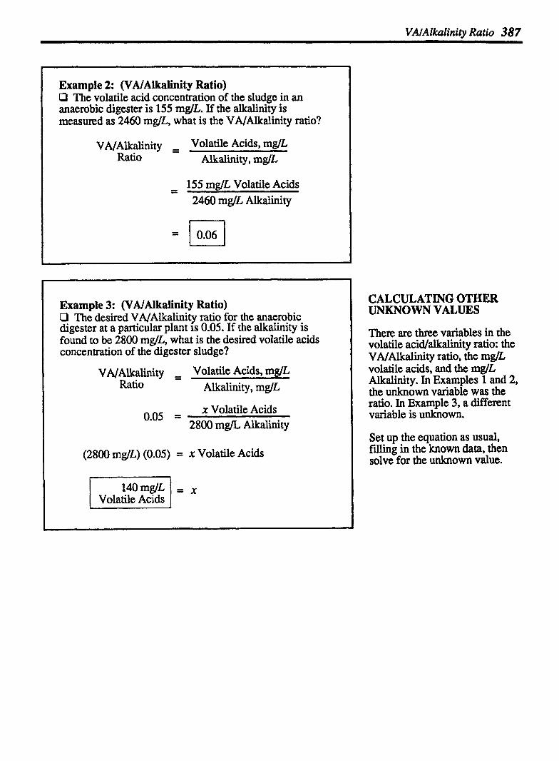
VAIAIkalinity Ratio 387
Example 2: (VA/Alkalinity Ratio) 0 The volatile acid concentration of the sludge in an anaerobic digester is 155 mg/L. If the alkalinity is measured as 2460 rnglL, what is the VA/Alkalinity ratio?
155 mg/L Volatile Acids 2460 mg/L Alkalinity
Example 3: (VNAlkalinity Ratio) 0 The desired VA/Alkalinity ratio for the anaerobic digester at a particular plant is 0.05. If the alkalinity is found to be 2800 m@, what is the desired volatile acids concentration of the digester sludge?
x Volatile Acids 0.05 =
2800 m& Alkalinity
(2800 mglL) (0.05) = x Volatile Acids
Volatile Acids
CALCULATING OTHER UNKNOWN VALUES
There are three variables in the volatile acid/alkalinity ratio: the VA/Alkalinity ratio, the mg/L volatile acids, and the mglL Alkalinity. In Examples 1 and 2, the unknown variable was the ratio. In Example 3, a different variable is unknown.
Set up the equation as usual, filling in the known data, then solve for the unknown value.
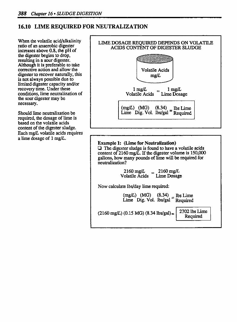
388 Chapter 16 SLUDGE DIGESTION
16.10 LIME REQUIRED FOR NEUTRALIZATION
When the volatile acid/alkalinity ratio of an anaerobic digester increases above 0.8, the pH of the digester begins to drop, resulting in a sour digester. Although it is preferable to take comctive action and allow the digester to recover naturally, this is not always possible due to limited digester capacity and/or recovery time. Under these conditions, lime neutralization of the sour digester may be necessary.
Should lime neutralization be required, the dosage of lime is based on the volatile acids content of the digester sludge. Each mglL volatile acids requires a lime dosage of 1 mglL.
LIME DOSAGE REQUIRED DEPENDS ON VOLATILE ACIDS CONTENT OF DIGESTER SLUDGE
I Volatile Acids I
l mg1L = 1 mg/L Volatile Acids Lime Dosage
Example l: (Lime for Neutralization) O The digester sludge is found to have a volatile acids content of 2160 mglL. If the digester volume is 150,000 gallons, how many pounds of lime will be required for neutralization?
2160mglL 2160mglL Volatile Acids Lime Dosage
Now calculate lbs/day lime required:
(2160 mglL) (0.15 MG) (8.34 lbs/gal)= I 270ig&ime 1
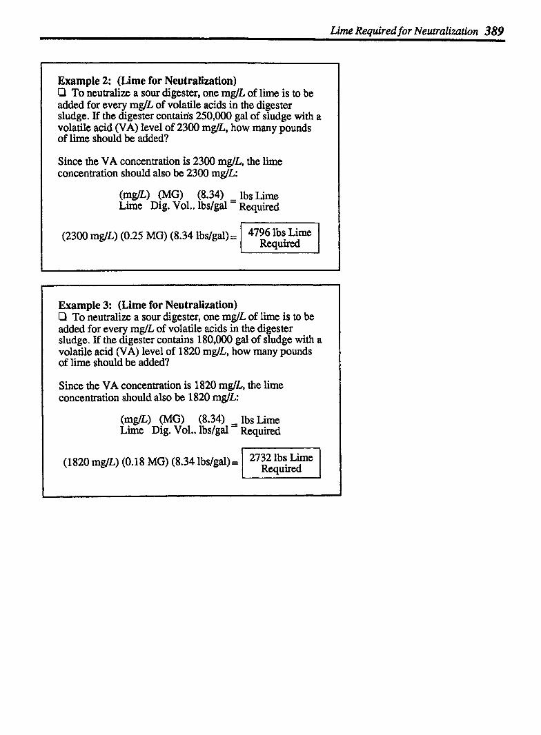
Lime Required for Neutralization 389
Example 2: (Lime for Neutralization) O To neutralize a sour digester, one mglL of lime is to be added for every mg/L of volatile acids in the digester sludge. If the digester contains 250,000 gal of sludge with a volatile acid (VA) level of 2300 mglL, how many pounds of lime should be added?
Since the VA concentration is 2300 mglL, the lime concentration should also be 2300 mdL:
(2300 mg/L) (0.25 MG) (8.34 lbslgal) = I 47y$!ne I
Example 3: (Lime for Neutralization) Cl To neutralize a sour digester, one mg/L of lime is to be added for every mglL of volatile acids in the digester sludge. If the digester contains 180,000 gal of sludge with a volatile acid (VA) level of 1820 mglL, how many pounds of lime should be added?
Since the VA concentration is 1820 mglL, the lime concentration should also be 1820 mglL:
(mg/L) (MG) (8.34) - lbs Lime Lime Dig. Vol.. lbs/gd - Required
(1820 mglL) (0.18 MG) (8.34 lbslgal) = I 2732Ekiime 1
390 Chapter 16 SLUDGE DIGESTION
16.11 PERCENT VOLATILE SOLIDS REDUCTION
One of the best indicators of the effectiveness of the digestion process is the volatile solids content of the digested sludge. This volatile content may be compared with the original volatile content of the influent sludge, and from the two values the percent volatile solids reduction due to digestion may be calculated. This reduction may be as high as 70%. When volatile solids data is given in lbs or lbs/da y, the percent volatile solids reduction calculation is similar to any other percent removal calculation:
% VS VS Removed, lbs 100 - Rem* VS Tot. Entering, lbs
In most volatile solids reduction calculations, however, the volatile solids data is given as percents. This creates a problem since the percents are based on different wholes (during digestion some of the volatile solids are converted to gases and water).
To remedy this problem, the equations shown to the right are used to calculate percent volatile solids reduction.
WHEN VOLATILE SOLIDS ARE EXPRESSED AS POUNDS, PERCENT VS REDUCTION IS A USUAL PERCENT CALC.
lbs VS , lbs VS Total Digester Leaving
Entering
lbs VS Reduced (or Destroyed)
% VS - - VS Reduced, lbs 100 Reduction Total VS Entering, lbs
WHEN VOLATILE SOLIDS ARE EXPRESSED AS PERCENTS A DIFFERENT EOUATION MUST BE USED
SOLIDS ENTERING SOLIDS LEAVING DIGESTION DIGESTION
If the VS entering the digester If the VS leaving the digester are 70%, the remaining solids are 40%, the remaining solidi W d solids) must be 30% Ifuced) must be 60%
Fixed solids normally remain relatively unchanged by digestion. Yet fixed solids are 30% in one case above and 60% in the other. This is because the percents are based on different wholes.
There are two equations that may be used to calculate percent volatile solids reduction when volatile solids are expressed as percents:.
% vs = (45 VS In - % VS Out) 100 Reduction % VS - (% VS) (% VS )
In In Out
In the equation shown below, the "In" and "Out" data are written as decimal fractions.*
% vs = In-Out x I W / Reduction In - (In X Out)
* For example, 70% VS entering the digester would be written as 0.70 and 56% VS leaving the digestex would be written as 0.56.
% VS Reduction 391
Example 1: (96 VS Reduction) O The sludge entering a digester has a volatile solids content of 70%. The sludge leaving the digester has a volatile solids content of 52%. What is the percent volatile solids reduction?
70% - Digester = 0.70 = 0.52
% VS = In-Out xlOO Reduction In - (In X Out)
To use this equation, express percents as decimal fkactions:
% vs = 0.70 - 0.52 X 100
Reduction 0.70 - (0.70 X 0.52)
= 1 54% VS Reduction 1
Example 2: (% VS Reduction) O The raw sludge to a di ester has a volatile solids content of 72%. The digested slu ge volatile solids content is 46%. What is the percent volatile solids reduction?
721 1 Digester I-* 46% = 0.72 = 0.46
% VS = In -Out Reduction In - (In X Out)
To use this equation, express percents as decimal fractions:
% vs = 0.72 - 0.46 X 100
Reduction 0.72 - (0.72 X 0.46)
= 1 67% VS Reduction I
392 Chapter l6 SLUDGE DIGESTION
16.12 VOLATILE SOLIDS DESTROYED, lbs VSIdaylcu ft
One measure of digester effectiveness is pounds of volatile solids reduced or destroyed per cubic feet of digester volume. The equations to be used in these calculations are shown to the right.
LBS/DAY VOLATILE SOLIDS DESTROYED PER CU FT DIGESTER VOLUME
lbs/day VS Reduction
Digester I volume I Simplified Equation:
VS Destroyed, lbs/day Destroyed, =
lbs VS/day /cu ft Dig* cu
Expanded Equation:
(gpd) (8.34) (% Sol.) (% VS)(% VS Red.)
Destroyed - 100 I lbs vs/day /cu ft - (0.785)(D2)(depth, ft) I
Example l: (Volatile Solids Destroyed) D A flow of 3300 gpd sludge is pumped to a 32,000 cu ft digester. The solids concentration of sludge is 6.3%, with a volatile solids content of 72%. If the volatile solids reduction during digestion is 5446, how many lbs/day volatile solids are destroyed per cu ft of digester capacity?
(gpd) (8.34) (% Sol.)(% VS)(% VS Red*) Sludge lbs/gal 100 Destroyed, 100
lbslday \iS/cu ft Digester Volume, cu ft
(3300 gpd) (8.34) (6.3) (72) (54) lbs/gal 100 100 100
- 0.021 lbs VS/day - l cu ft
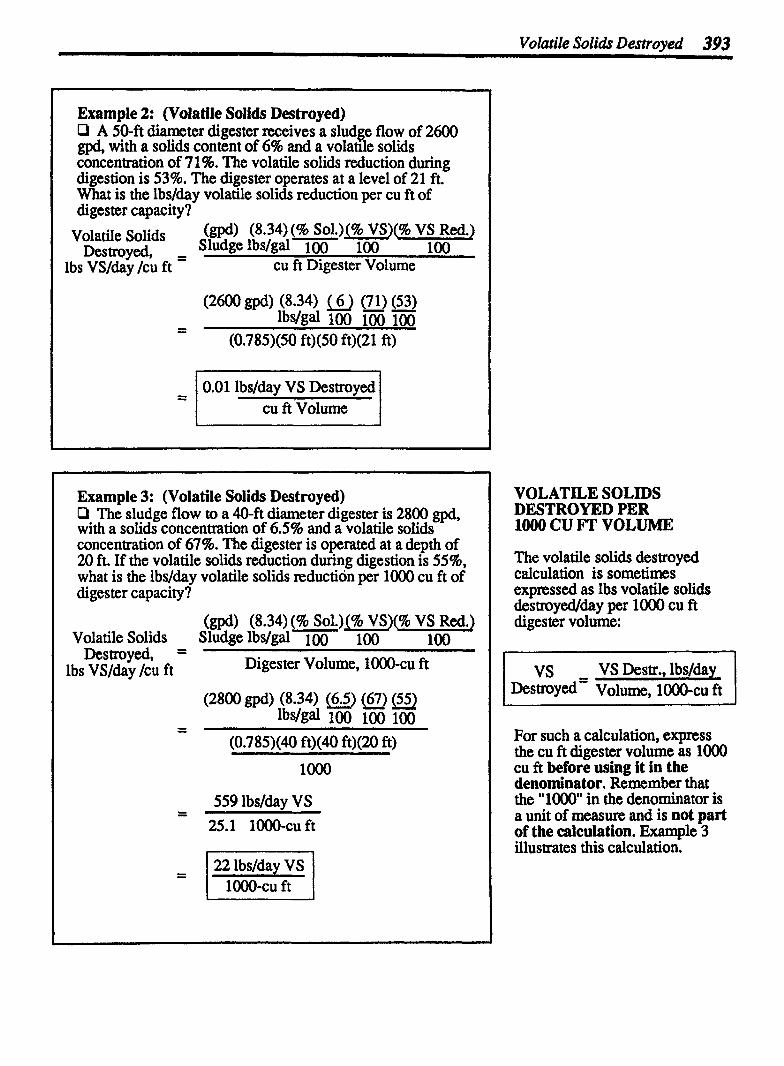
Volatile Solidr Destroyed 393
Example 2: (Volatile Solids Destroyed) O A 50-ft diamter digester receives a sludge flow of 2600 gpd, with a solids content of 6% and a volatlle solids concentration of 7 1 %. The volatile solids reduction during digestion is 53%. The digester operates at a level of 21 ft. What is the lbslday volatile solids reduction per cu ft of digester capacity?
(gpd) (8.34) (% Sol.) (% VS)(% VS Red.) "laae "lids Sludge lbslgal 100 Desbroved, - 100
lbs VS/&~ lcu ft - cu ft Digester Volume
- (0.785)(50 ft)(50 ft)(21 ft)
= 1 0.01 lbs/&y VS Destroyed cu ft Volume
Example 3: (Volatile Solids Destroyed) P The sludge flow to a 40-ft diameter digester is 2800 gpd, with a solids concentration of 6.5% and a volatile solids concentration of 67%. The digester is operated at a depth of 20 ft. If the volatile solids reduction during digestion is 55%. what is the lbs/day volatile solids reduction per 1000 cu ft of digester capacity?
(gpd) (8.34) (% Sol.) (% VS)(% VS Red.) Volatile Solids Sludge l b s / g a l ~ 10 100
Destroyed, = lbs VS/day /cu ft Digester Volume, 1000-cu ft
(2800 gpd) (8.34) ( 5 ) (67) (55) lbslgal 100 100 100 -
(0.785)(40 ft)(40 ft)(20 ft)
VOLATILE SOLIDS DESTROYED PER 1O00 CU FT VOLUME
The volatile solids destroyed calculation is sometimes expressed as lbs volatile solids destroyed/day per loo0 cu ft digester volume:
For such a calculation, express the cu ft digester volume as 1OO0 cu ft before using it in the denominator. Remember that the "1000 in the denominator is a unit of measure and is not part of the calculation. Example 3 illustrates this calculation.
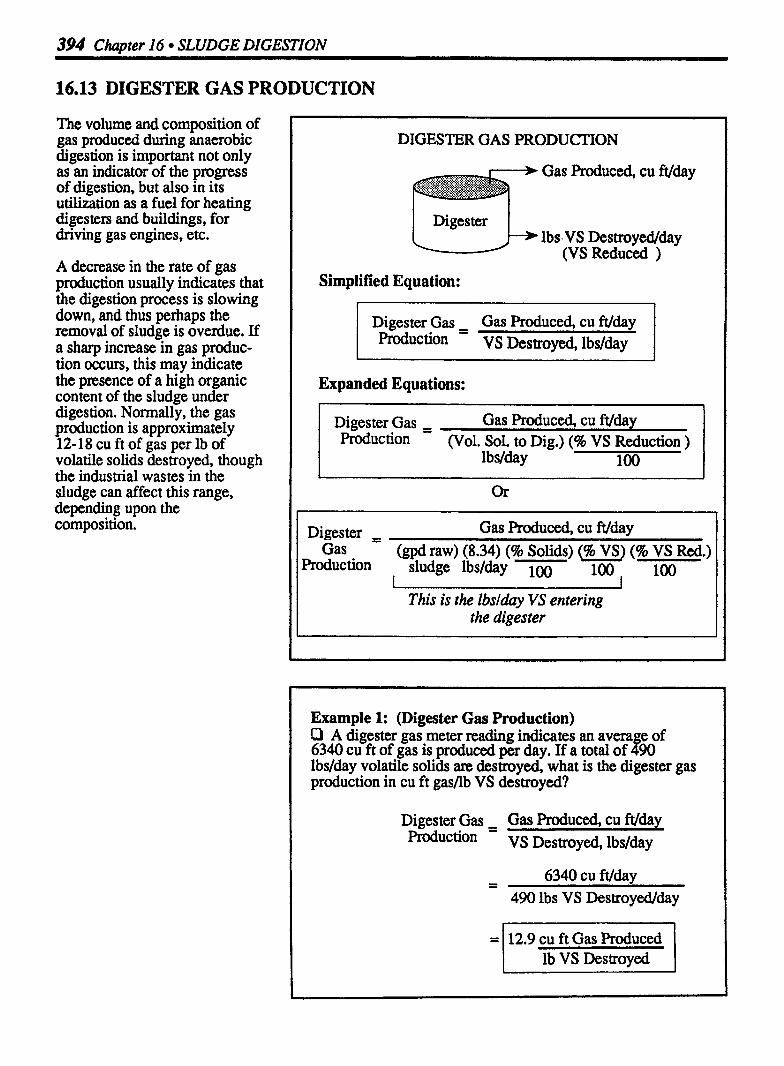
394 Chapter 16 SLUDGE DIGESTION
16.13 DIGESTER GAS PRODUCTION
The volume and composition of gas produced during anaerobic digestion is important not only as an indicator of the progress of digestion, but also in its utilization as a fuel for heating digesters and buildings, for driving gas engines, etc.
A decrease in the rate of gas production usually indicates that the digestion process is slowing down, and thus perhaps the removal of sludge is overdue. If a sharp increase in gas produc- tion occurs, this may indicate the presence of a high organic content of the sludge under digestion. Normally, the gas production is approximately 12-18 cu ft of gas per lb of volatile solids destroyed, though the industrial wastes in the sludge can affect this range, depending upon the composition.
DIGESTER GAS PRODUCTION
Simplified Equation:
Digester Gas - Gas Produced, cu ftlday - Pmiucti0* VS Destroyed, lbsfday
Expanded Equations:
I Digester Gas = Gas Produced, cu Wday I - production (Vol. Sol. to Dig.) (% VS Reduction )
lbs/day loo
Digester , - Gas Produced, cu Wday Gas (gpd raw) (8.34) (% Solids) (% VS) (96 VS Red.)
P-mduction sludge lbslday 100 100 , 100 - - -
This is the lbslday VS entering the digester
Example 1: (Digester Gas Production) P A digester gas meter reading indicates an avera e of f 6340 cu ft of gas is produced per day. If a total of 90 lbs/day volatile solids are destroyed, what is the digester gas production in cu ft gasfib VS destroyed?
Digester Gas - - Gas Produced, cu ft/day Production VS Destroyed, lbslday
-
490 lbs VS Destroyed/day - - P - - - P -
= 12.9 cu ft Gas Produced ( lb VS Destroyed

Digester Gas Production 395
Example 2: (Digester Gas Production) D A total of 1900 lbs of volatile solids are umped to the 9 digester daily. If the percent reduction of vo atile solids due to digestion is 60% and the average gas production for the day is 18,240 cu ft, what is the daily gas production in cu ft/lb VS destroyed daily?
Digester Gas - - Gas Produced, cu ft/day Production (Vol. Sol. to Dig.) (% VS Reduction )
18.240 cu ft Gas Producedldav
= 1 16 cu ft Gas Produced lb VS Destroyed
Example 3: (Digester Gas Production) O The anaerobic di ester at a plant receives a total of f 11,400 gpd of raw S udge. This sludge has a solids content of 5.496, of which 62% is volatile. If the digester yields a volatile solids reduction of 5846, and the average digester gas production is 25,850 cu ft, what is the daily gas production in cu frflb VS destroyed?
Digester , Gas Produced, cu ft/day -
Gas (gpd raw) (8.34) (46 Solids) (% VS) (% VS Red.) Production sludge lbslday 100 100 ,
I 100
This is the ibslday VS entering the digester
25,850 cu ft Gas Produced/da~ - (1 1,400 gpd) (8.34*) ( 5.4 ) ( 62 ) ( 58 ) raw sludge lbslgal l()() 100 100
14 cu ft Gas Produced lb VS Destroyed
* If the sludge has a higher density than water, a number greater than 8.34 lbs/gal should be used here. Refer to Chapter 7 for a discussion of density and specific gravity.
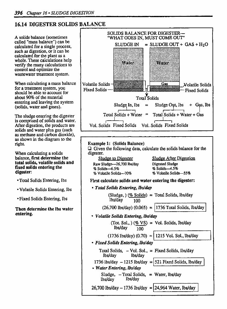
396 Cha~ter l6 SLUDGE DIGESTION
16.14 DIGESTER SOLIDS BALANCE
A solids balance (sometimes called "mass balance") can be calculated for a single process, such as digestion, or it can be calculated for the plant as a whole. These calculations help verify the many calculations to control and optimize the wastewater treatment system.
When calculating a mass balance for a treatment system, you should be able to account for about 90% of the material entering and leaving the system (solids, water and gases).
The sludge entering the digester is comprised of solids and water. After digestion, the products are solids and water plus gas (such as methane and carbon dioxide), as shown in the diagram to the right.
When calculating a solids balance, first determine the total solids, volatile solids and fixed solids entering the digester:
Total Solids Entering, lbs
Volatile Solids Entering, lbs
. Fixed Solids Entering, lbs
Then determine the Ibs water entering.
s o L m s BALANCE FOR DIGESTER- "WHAT GOES IN, MUST COME OUT"
SLUDGE IN = SLUDGE OUT + GAS + H20
v Total Solids
Sludge In, lbs = A
Total Solids + Water = Total Solids + Water + Gas 47 47
Vol. Solids Fixed Solids Vol. Solids Fixed Solids
Example 1: (Solids Balance) C1 Given the following data, calculate the solids balance for the digester.
Sludee to Digester Sludge After Digestion Raw S ludge-26,700 lbs/day Digested Sludge % S o l i d M S % % Sol iddS% % Volatile Solido70% % Volatile Solids-55%
First calculate solids and water entering the digester: Total Solids Entering, lbslday
(Sludge, ) (% Solids) = Total Solids, lbslday Wday 100
P 1
(26,700 lbslday) (0.065) = 11736 Total Solids, lbslday I Volatile Solids Entering, lbsldoy
(Tot. Sol., ) (% - VS) = Vol. Solids, lbs/day lbslday 100
I 1
I I
Fixed Solids Entering, lbslday
26,700 lbs/day - 1736 lbslday = 124,964 Water, lbs/day I
Total Solids, - Vol. Sol., = Fixed Solids, lbs/day l bslda y l bslday
1736 lbslday - 1215 lbslday = 521 Fixed Solids, lbslday Water Entering, ibs/&zy
L
Sludge, - Total Solids, = Water, lbslday lbs/da y lbsfday

Digester Solids Balance 397
Then calculate solids, water and gas leaving the digester: (To begin these calculations, you must first determine the percent volatile solids reduction during digestion.
% Volatile Solids Reduction* (Write percents as decimd fractbns)
% VS = In-Out xlOO Reduction In - (In X Out)
-
= 147.6% VS Reduction I Gas Produced, lbslday (VS destroyed or reduced = lbs gas produced)
(VS Entering Digester) (% VS Reduction) - - Gas Produced l bslday 100 l b slday
(1215 lbslday Vol. Sol.) (0.476) = I 578 lbslday Gas Produced
Volatile Solids in Digested Sludge, lbslday VS Entering Digester - VS Destroyed = VS Leaving
l b S/& y l b slda y Digester, lbs/day
12151bs1day- 5781bs/day =
Total Solids in Digested Sludge, lbslday Vol. Sol., lbslday
% vs = Total Solids, lbslday
100
Fixed Solids in Digested Sludge, lbsldny
637 lbsIday A C: VS =
Tot. Sol., lbslday - VS, lbslday = Fixed Solids, lbslday
1 158 lbslday Total Solids
Digested Sludge, lbslday
So'ids' lbs/day = Digested Sludge, lbslday % Solids
lbslday n n ~ c Tot* "l* = ' 25,733 lbslday Digested Sludge
Water in Digested Sludge, lbslday
Sludge, lbslday -Total Solids, lbslday = Water, lbslday
To account for solids leaving the digester, you will makc the same basic calculations but in a slightly different order. You must begin by determining the % volatile solids reduction, then calculate the solids, water, and gas, as shown in the example calculation.
Sludge Entering Sludge Leaving
Tot. Sol.-1736 1bs (VS-1215 lbs) (FS- 521 lbs)
* For a review of the percent volatile solids reduction calculation, refer to Section 16.1 1.
Tot. Sol.1158 lbs (VS--637 lbs) (FS- 521 lbs)
Water-24,964 1bs 26,700 1bs
Water-24,575 1bs Gas- 578 1bs
26,3 1 1 lbs
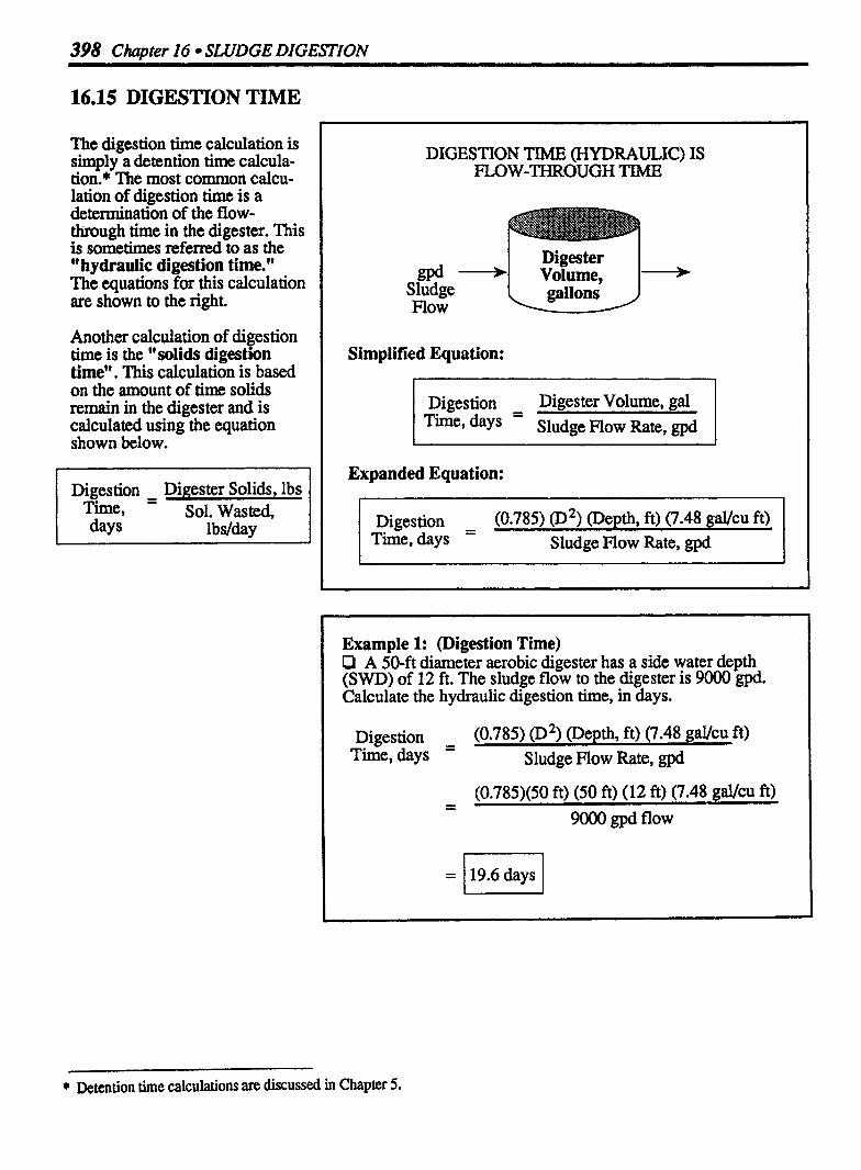
398 Chapter I6 SLUDGE DIGESTION
16.15 DIGESTION TIME
The digestion time calculation is simply a detention time calcula- tion.* The most common calcu- lation of digestion time is a determination of the flow- through time in the digester. This is sometimes r e f e d to as the l' hydraulic digestion time." The equations for this calculation are shown to the right.
Another calculation of digestion time is the " solids digestion time". This calculation is based on the amount of time solids remain in the digester and is calculated using the equation shown below.
Digestion - Digester Solids, lbs Time, - Sol. Wasted, days lbdday
DIGESTION TIME (HYDRAULIC) IS FLOW-THROUGH TIME
Digester
Sludge Flow
Simplified Equation:
Digestion Digester Volume, gal - - Sludge Flow Rate, gpd
Expanded Equation:
Digestion - - (0.785) (D2) (Depth, ft) (7.48 gaVcu ft) Time, days Sludge Flow Rate, gpd
Example 1: (Digestion Time) P A 50-ft diameter aerobic digester has a side water depth (SWD) of 12 ft. The sludge flow to the digester is 9000 gpd. Calculate the hydraulic digestion time, in days.
Digestion - - (0.785) (D 2, (Depth, ft) (7.48 gaVcu ft) Time, days Sludge Flow Rate, gpd
- - (0.785)(50 ft) (50 ft) (12 ft) (7.48 gUcu ft) 9000 gpd flow
= 1 19.6 days I
* Detention time calculations are discussed in Chapter 5.
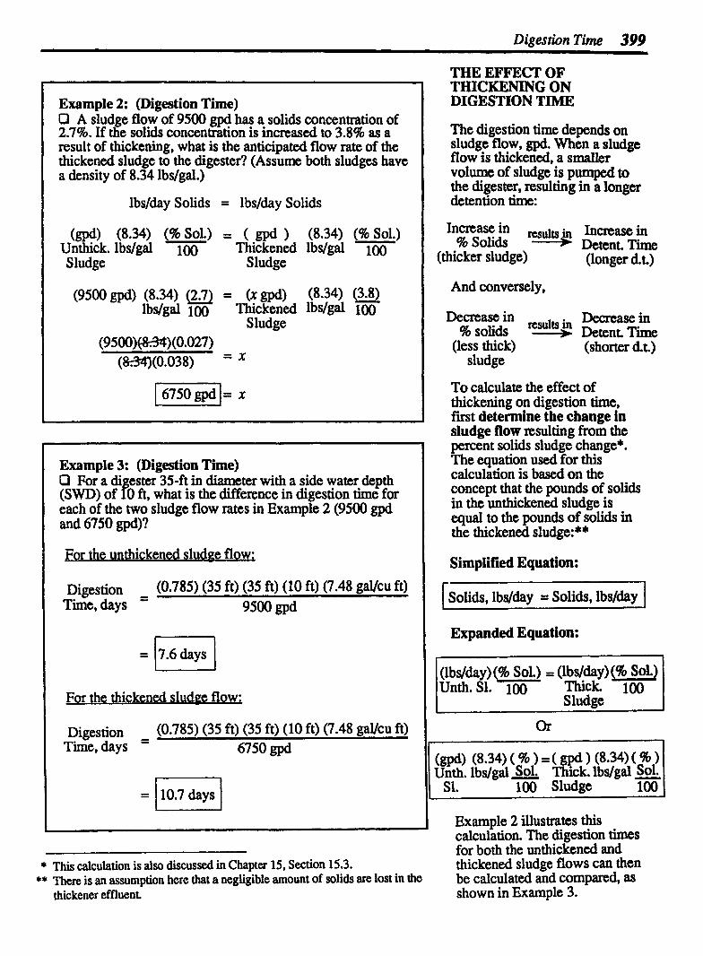
Digestion Time 399
Example 2: (Digestion Time) P A sludge flow of 9500 gpd has a solids concentration of 2.7%. If the solids concentration is increased to 3.8% as a
, result of thickening, what is the anticipated flow rate of the thickened sludge to the digester? (Assume both sludges have a density of 8.34 lbs/gal.)
lbs/day Solids = lbs/day Solids
(gpd) (8.34) = ( gpd ) (8.34) (% Sol.) Unthick. lbslgal 100 Thickened lbs/gal 100
I Sludge Sludge
l (9500 gpd) (8.34) (2.7) = (X gpd) (8.34) (3.8) lbs/gal 100 Thickened lbs/gal 100
l Sludge (9500)&34) (0.027)
(&34)(0.038) = X
Example 3: (Digestion Time) P For a di ester 35-ft in diameter with a side water depth (SWD) of f;O ft, what is the difference in digestion time for each of the two sludge flow rates in Example 2 (9500 gpd and 6750 gpd)? r
I For the unthickened sludge flow; I Digestion (0.785) (35 ft) (35 ft) (10 ft) (7.48 gaku ft) Time, days -
9500 gpd
I Forth e thickened sludge flow;
= 10.7 days I * This calculation is also discussed in Chapter 15, Section 15.3.
THE EFFECT OF THICKENING ON DIGESTION TIME
The digestion time depends on sludge flow, gpd. When a sludge flow is thickened, a smaller volume of sludge is pumped to the digester, resulting in a longer detention time:
And conversely,
in results in Decrease in % solids + Detent. Time (less thick) (shorter dt.)
sludge
To calculate the effect of thickening on digestion t h e , fust determine the change in sludge flow resulting from the percent solids sludge change*. The equation used for this calculation is based on the concept that the pounds of solids in the unthickened sludge is equal to the pounds of solids in the thickened sludge: * * Simplified Equation:
(S&&, lbs/day = Solids, lbs/day 1 Expanded Equation:
(lbdday) (% Sol.) (lbdday) (% SOL) Unth. S1. 100 Thick. 100
Sludge
Example 2 illustrates this calculation. The digestion times for both the unthickened and thickened sludge flows can then
** There is an assumption here that a negligible amount of solids are lost in the be calculated &d compared, as thickener effluent. shown in Example 3.
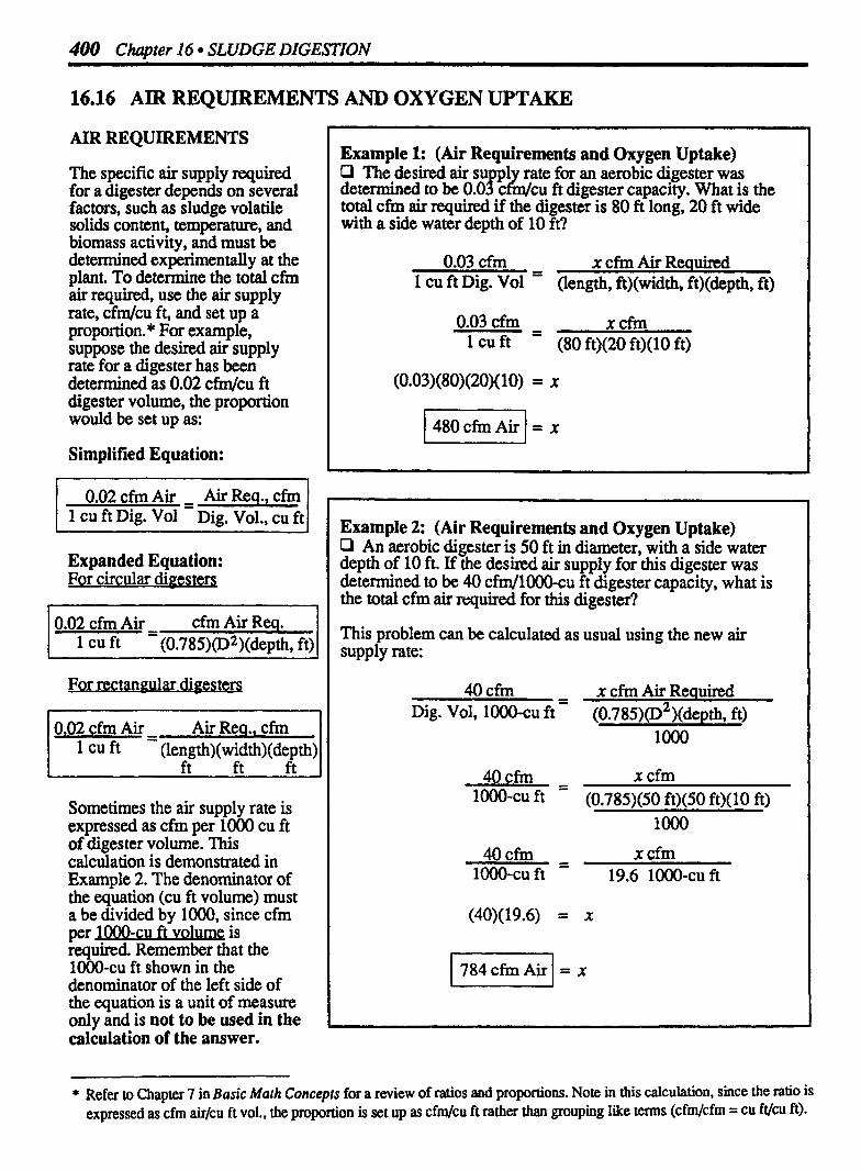
400 Chapter 16 SLUDGE DIGESTION
16.16 AIR REQUIREMENTS AND OXYGEN UPTAKE
AIR REQUIREMENTS
The specific air supply required for a digester depends on several factors, such as sludge volatile solids content, temperature, and biomass activity, and must be determined experimentally at the plant. To determine the total cfin air required, use the air supply rate, cfdcu ft, and set up a proponion. * For example, suppose the desired air supply rate for a digester has been determined as 0.02 c w c u ft digester volume, the proportion would be set up as:
Simplified Equation:
0.02 cfrn Air - Air Req., cfm 1 cu ft Dig. Vol - Dig. Vol., cu ft
Expanded Equation: For circular digesters
0.02 cfrn Air - - cfrn Air Req. 1 cu ft (Oe785)@2)(depth, ft) 1 or rectangular digesters
0.02 cfrn Air - - Air Req., cfrn 1 cu ft (length)(width)(depth)
ft ft ft
Sometimes the air supply rate is expressed as cfrn per 1000 cu ft of digester volume. This calculation is demonstrated in Example 2. The denominator of the equation (cu ft volume) must a be divided by 1000, since cfrn per m - c u ft volume is required. Remember that the 1000-cu ft shown in the denominator of the left side of the equation is a unit of measure only and is not to be used in the calculation of the answer.
Example l: (Air Requirements and Oxygen Uptake) O The desired at su p1 rate for an aerobic digester was determined to be 0.0 f & c cu ft digester capacity. What is the total cfm air required if the digester is 80 ft long, 20 ft wide with a side water depth of 10 ft?
0.03 cfrn - X cfrn Air Required l cu ft Dig. Vol - (length, ft)(width, ft)(depth, ft)
0.03 cfm X cfm 1 cu ft - (80 ft)(20 ft)(lO ft)
Example 2: (Air Requirements and Oxygen Uptake) Cl An aerobic digester is 50 ft in diameter, with a side watex depth of 10 ft. If the desired air supply for this digester was determined to be 40 cfm/1000cu ft digester capacity, what is the total cfrn air required for this digester?
This problem can be calculated as usual using the new air supply rate:
40 cfin x cfm Air Required Dig. Vol, 10OO-c~ ft - (0.785)(~~)(de~th, ft)
loo0
4 0 c h - - X cfrn 1OOo-cu ft (0.785)(50 ft)(50 ft)(lO ft)
4 0 c h - X cfm ~OOO-CU ft 19.6 1000-cu ft
* Refer to Chapter 7 in Basic Moth Concepts for a review of ratios and proportions. Note in this calculation, since the ratio is expressed as cfrn air/cu ft vol., the proportion is set up as c f d c u ft rather than grouping like terns (cfm/cfm = cu ft/cu ft).

Air Requirements and Oxynen Uvtake 401
Example 3: (Air Requirements and Oxygen Uptake) D The dissolved air concentrations recorded during a 5-minute test of an air-saturated sample of aerobic digester sludge are given below. Calculate the oxygen uptake, in mg/"/'r*
Elapsed Elapsed Time, min D.O., mdL Time, min D.O., m&
At Start 6.9 3 min 4.3 1 min 5.8 4 min 3.7 2 min 5 .O 5 min 2.9
- 0 2 uptake, - - at-2 min. at5 min. 60 min
m g L b 5 min - 2 min hr
- - 5.0 mgIL - 2.9 mglL 60 rnin - 3 min hr
Example 4: (Air Requirements and Oxygen Uptake) Q Dissolved air concentrations are taken at one-minute intervals on an air-saturated sample of digester sludge. Given the results below, calculate the oxygen uptake, in mg/L/hr-
Elapsed Elapsed Time, min D.O., mg/L Time, min D.O., mdL
At Start 7.3 3 min 4.9 1 min 6.4 4 min 4.1 2 min 5.6 5 min 3.2
mg/LDO - mglLD0 0 2 uptake, - at 2 min. at 5 min. ,60 min
mg/L/hr 5 min - 2 min hr
- 5.6 mglL - 3.2 mglL 60 min -. - 3 min hr
OXYGEN UPTAKE
Another measurement of the aerobic digestion system is oxygen air uptake. The oxygen uptake is an indication of microbiological (biomass) activity. Then is an inmase in oxygen uptake with increased microorganism activity ; and there is a decrease in oxygen uptake when the biomass activity slows (such as during upset conditions).
To determine oxygen uptake, a one-liter sample of digested sludge is tested for dissolved oxygen (DO) levels. The DO measurement is recorded at the start of the test and at one-minute intervals for the duration of the five-minute test.
The DO measurements at 2 minutes and 5 minutes are generally used to calculate the oxygen uptake.
Simplified Equation:
I mdL DO used I 0 2 Uptake, during Test 60 min 1 / -Min. during hr
I Measurement I
Expanded Equation:
For measurements taken at times other than 2 a d 5 minutes, use the following general equation:
Expanded Equation:
l min min
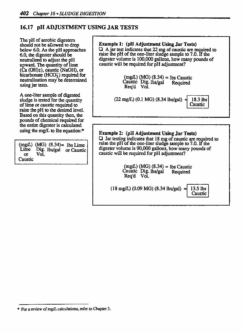
402 Chapter I6 SLUDGE DIGESTION
16.17 pH ADJUSTMENT USING JAR TESTS
The pH of aerobic digesters should not be allowed to drop below 6.0. As the pH approaches 6.0, the digester should be neutralized to adjust the pH upward. The quantity of lime (Ca (OH)?), caustic (NaOH), or bicarbonate WC%) required for neutralization may be determined using jar tests.
A one-liter sample of digested sludge is tested for the quantity of lime or caustic required to raise the pH to the desired level. Based on this quantity then, the pounds of chemical required for the entire digester is calculated using the mg/L to lbs equation:*
(m&) (MG) (8.34)= lbs Lime Lime Dig. lbslgal or Caustic
or Vol. Caustic
Example 1: (pH Adjustment Using Jar Tests) D A jar test indicates that 22 m of caustic are uired to raise the pH of the one-liter slu c f ge sample to 7 . 0 3 the digester volume is 100,000 gallons, how many pounds of caustic will be required for pH adjustment?
(22 mglL) (0.1 MG) (8.34 lbslgal) 1 8.3 lbs 1 Caustic I
Example 2: (pa Adjustment Using Jar Tests) P Jar testing indicates that 18 mg of caustic are raise the pH of the one-liter sludge sample to 7.0. ?F to digester volume is 90,000 gallons, how many pounds of caustic will be required for pH adjustment?
(m@) (MG) (8.34) = Ibs Caustic Caustic Dig. lbslgal Rquired Req'd Vol.
(18 mglL) (0.09 MG) (8.34 lbs/gal) = Caustic
* For a review of mg/L calculations, refer to Chapter 3.
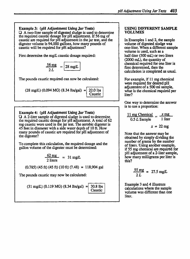
pH Adjustment Using Jar Tests 403
Example 3: (pH Adjustment Using Jar Tests) P A two-liter sample of digested sludge is used to determine the required caustic dosage for pH adjustment. If 56 mg of caustic are required for pH adjustment in the jar test, and the digester volume is 94,000 gallons, how many pounds of caustic will be required for pH adjustment?
First determine the mg/L caustic dosage requid:
The pounds caustic required can now be calculated:
(28 mglL) (0.094 MG) (8.34 lbslgal) = 22.0 lbs / caustic I
Example 4: (pH Adjustment Using Jar Tests) O A 2-liter sample of digested sludge is used to determine the required caustic dosage for pH adjustment. A total of 62 mg caustic were used in the jar test. The aerobic digester is 45 feet in diameter with a side water depth of 10 ft. How many pounds of caustic are required for pH adjustment of the digester?
To complete this calculation, the required dosage and the gallon volume of the digester must be determined:
62 mg = 31 mglL 2 liters
(0.785) (45 ft) (45 ft) (10 ft) (7.48) = 118,904 gal
The pounds caustic may now be calculated:
(31 mglL) (0.119 MG) (8.34 lbslgal) = Caustic
USING DIFFERENT SAMPLE VOLUMES
In Examples 1 and 2, the sample volume of digested sludge was one-liter. When a different sample volume is used, such as a half-liter (500 d) or two liters (2000 mL), the quantity of chemical required for one liter is first determined, then the calculation is completed as usual.
For example, if 11 mg chemical were required for desired pH adjustment of a 500 m1 sample, what is the chemical required per liter?
One way to determine the answer is to use a proportion:
l l mg Chemical - X mg - 0.5 L Sample 1 liter
Note that the answer may be obtained by simply dividing the number of grams by the number of liters. Using another example, if 55 mg chemical are required for pH adjustment of a 2-liter sample, how many milligrams per liter is this?
Example 3 and 4 illustrate calculations where the sample volume was different than one liter.


1 7 Sludge Dewatering and Disposal
1. Filter Press Dewatering
Solids Loading Rate-Plate and Frame Filter Press
Simolified Equation;
Solids Loading - Solids, lbs/hr Rate, lbslhr/sq ft - Plate Area, sq ft
Ex~anded Equation;
( e h ) (8.34) (% Sol.) Solids Loading - Sludge lbslgal 100
Rate, lbs/hr/sq ft - Plate Area, sq ft
Net Filter Press-Plate and Frame Filter Press
Sim~li fied Equation:
Net Filter Yield, - (lbs/hr Sol.) (Filtration Run Time, hrs) I lbs/hr/sq ft -
Sq ft Total Cycle Time, hrs
Expanded Eauation;
2. Belt Filter Press Dewatering
Hydraulic Loading Rate
Hydraulic Loading - Flow, gPm Rate, gpmlft Belt Width, ft

406 Chapter 17 SLUDGE DEWATERING AND DISPOSAL
Sludge Feed Rate
I Sludge Feed Sludge to be Dewatered, lbs/day Rate, lbs/hr - Operating Time, hrdday I
Solids Loading Rate
e TSS data is Piven as percent
Solids Loading = (Sludge) (60 min) (8 .34m (96 TSS) Rate, lbs/hr Feed, hr gal 100
H'm
If the TSS data is eiven as m-&
Solids Loading = (mg/L) (MGD) (8.34&) Rate, lbs/hr TSS Sludge - - gal
Feed 24 hrs/&y
Solids loadin e rate is sometimes ex yessed as tonsh;
(Sludge) (60 min) (8.34 lbs)(% TSS) Feed
Solids Loading hr gal 100
Rate, tons/hr
Flocculant Feed Rate --
Flocculant = (mg/L) (MGD) (8.34!bs) Feed, lbsfhr Flocc. Feed
Rate gal
24 hrs/&y
Total Suspended Wids
Total Residue, - Total Filterable = Total Non-Filterable Residue, m& Residue, mglL

3. Vacuum Filter Dewatering
Filter Loading
Simdified Equation;
Filter Loading - Solids to Filter, lbs/hr lbs/hr/sq ft - Surface Area, sq ft
Ex~anded Eauation;
Sol. to Filter, lbslday Filter Loading Filter Oper., hrslday
lbs/hr/sq ft ' (nD)(width, ft)
Filter Yield If lbshr wet cake flow, percent cake solids, and filter area are used to calculate filter yield:
simplified Equation;
Filter Yield Dry Solids in Cake, lbshr lbshrlsq ft = Filter Area, sq ft
Ex~anded Eauation;
(Wet Cake Flow, lbs/hr)(% Solids in Cake) I Filter Yield 1~ ( lbslhrlsq ft =
* V W
Filter Area, sq ft I If filter loading (lbs/hr/sq ft) and percent solids recovery are used to calculate filter yield:
S imdified Equation:
Filter Yield (Filter Loading,) 1% Recovery) lbshdsq ft = lbs/hr/sq ft 100
Ex~anded Eauation:
Filter Area, sq ft IW
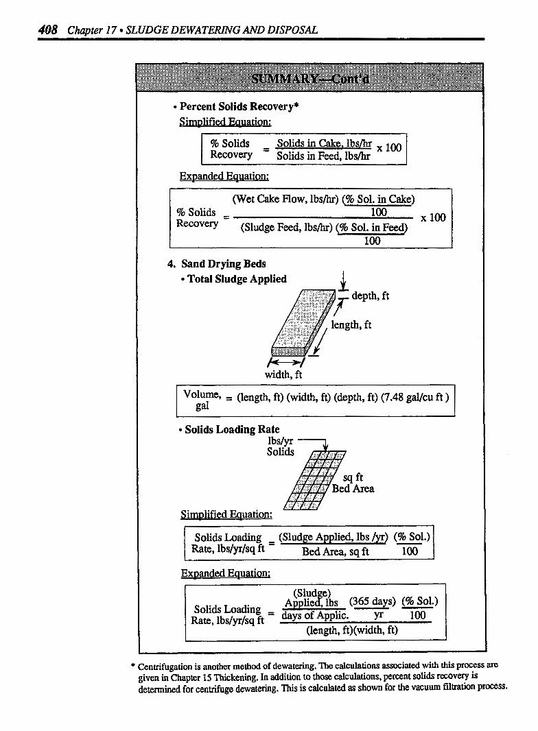
408 Chanter 17 SLUDGE DEWATERING AND DISPOSAL
Percent Solids Recovery* S im~lifed Equation:
% Solids - - Solids in Cake. lbs/hr 100 1 Recovery Solids in Feed, lbs/hr
Expanded Equation:
(Wet Cake Flow, Ibs/hr) (% Sol. in Cake) % Solids , - - 100
X 100 Kecovev (Sludge Feed, lbs/hr) (% Sol. in Feed)
4. Sand Drying Beds Total Sludge Applied
ength, ft
-/ width, ft
Solids Loading Rate
Sim~lified Equation:
, ft Area
Solids Loading - (Sludge Applied, lbs /yr) (95 Sol.) Rate, lbslyrlsq ft - Bed Area, sq ft 100 - l
Ex~anded Equation;
( s l u y ) ( Applie lbs 365 days) p (% $01.)
Solids Loading = days of ApPlic. Rate, lbs/yr/sq ft yr 100
(length, ft)(width, ft)
* Centrifugation is another method of dewatering. The calculations associated with this process are given in Chapter 15 Thickening. In addition to those calculations, percent solids recovery is determined for centrifuge dewatering. This is calculated as shown for the vacuum filtration process.
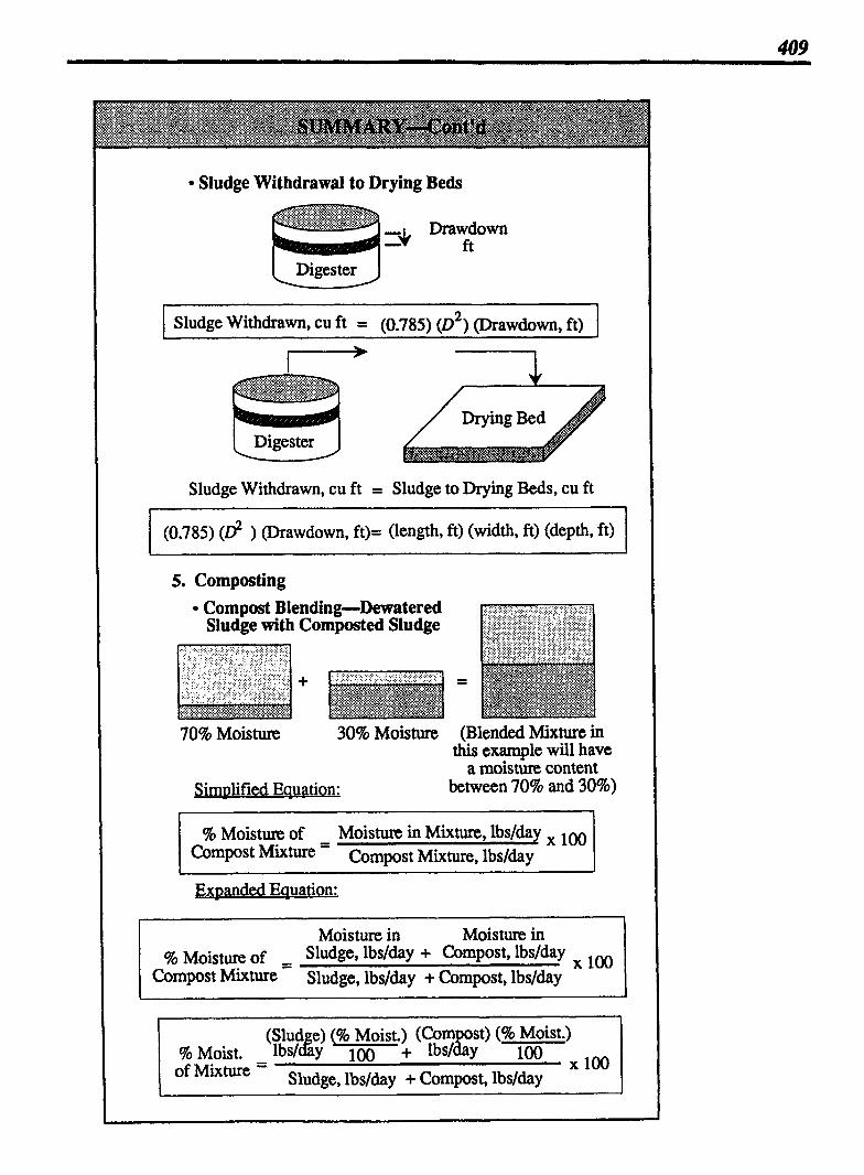
Sludge Withdrawal to Drying Beds
Sludge Withdrawn, cu ft = Sludge to Drying Beds, cu ft
l S. Cornposting
70% Moisture 30% Moisture (Blended Mixture in
Simplified Eauation:
this example will have a moisture content
between 70% and 30%)
% Moisture of Moisture in Mixture, lbslday 100 ComPOst = Compost Mixture, lbslday
Ex~anded Eauation:
(Slud c) (% Moist.) (Corn st) (% Moist.) - g %Moist. lbs/& 100 + l b ~ / y loo *loo of Mixture - Sludge, lbs/day + Compost, lbslday

41 0 Chapter 17 SLUDGE DEWATERING AND DISPOSAL
Compost Blending-Dewatered Sludge with Wood Chips
Simplified Equation:
% Solids of - Solids in Compost Blend, lbs 100 I -POSt Compost Blend, lbs
Expanded Equations:
% Solids Solids in + Solids in Wood of Compost = Sludge, lbs Chips, lbs
X 100
I Blend Sludge, lbs + Wood Chips, lbs I
% Solids of =
Compost 1 Blend
(Solids in) ( lbs ) (Solids in) ( lbs ) Sludge, - + wood chips, -=i cu yds cu yds
(Sludge,) ( lbs (Wood Chips,) ( lbs ) C U Y ~ c u d
- cu yds cu yd
(Sludge, )( lbs ) (%I Sol.) (Wood) ( lbs ) (96 Sol.) - -- % cu yds cu yd 100 + chips, cu yd 100 Solids cu yds of = X loo
compost (Sludge,) ( lbs k (Wood Chips,) ( - lbs Blend cu yds cu yd cu yds cu yd
Cu yds wood chips depends on the mix ratio* of wood chips to sludge
r------- I 1
(Sludge,) ( - lbs ) (96 Sol.) (Sludge,) (Mix) ( lbs ) (% Sol.) of + cu yds Ratio ,Yd
yds yd Sludge of
W.Chips % Solids
of = 100 loo X loo
Compost Blend
(Sludge) ( ) + (Sludge) ( Mix) ( lbs ) C U Y ~ cu yd cu yds Ratio cu yd
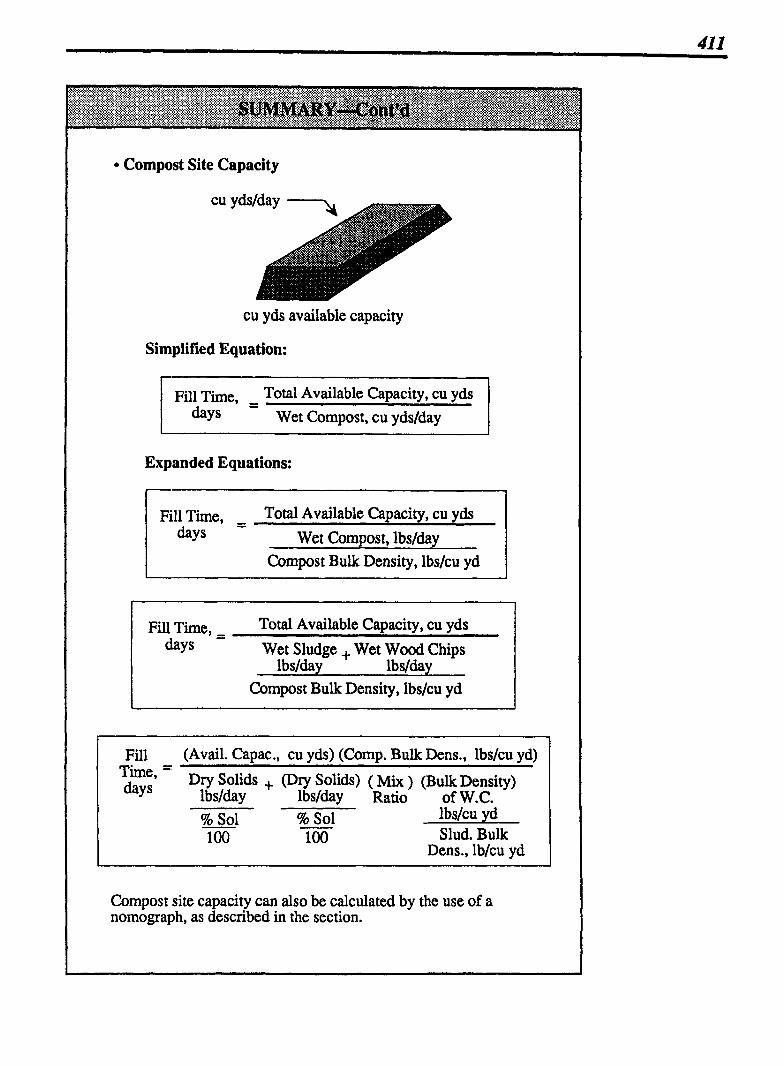
Compost Site Capacity
cu yds available capacity
Simplified Equation:
Fill Time, - Total Available Capacity, cu yds days
- Wet Compost, cu ydslday
Expanded Equations:
Fill Time, - - Total Available Capacity, cu yds days Wet Compost, lbs/day
Compost Bulk Density, lbs/cu yd
Fill Time, - - Total Available Capacity, cu yds days Wet Sludge + Wet Wood Chips
Ibslday lbslday Compost Bulk Density, lbs/cu yd
Fill (Avail. Capac., cu yds) (Comp. Bulk Dens., lbs/cu yd)
% Sol 100
% Sol 100
lbs/cu yd Slud. Bulk
Dens., lb/cu yd
Compost site capacity can also be calculated by the use of a nornograph, as described in the section.

412 Chapter 17 SLUDGE DEWATERING AND DISPOSAL
17.1 FILTER PRESS DEWATERING CALCULATIONS (PLATE AND FRAME FILTER PRESS)
SOLIDS LOADING RATE
The solids loading rate is an iniportant calculation in plate and frame fdter press operation. It is a measure of the lbs/hr solids applied per square foot of plate area, as shown in the box to the right.
Simplified Equation:
Solids Loading - Solids, lbs/hr Rate, lbs/hr/sq ft - Plate Area, sq ft
Expanded Equation:
,,-l (gph) (8.34) (% sol.)( I Sol*IUm Sludge lbslgal 100 1 Rate. -
Examples 1 and 2 illustrate this calculation.
Example 1: (Filter Press Dewatering) Cl A filter ress used to dewater digested primary sludge receives a 8 ow of 720 gallons during a 2-hr period. The sludge has a solids content of 3.5%. If the plate surface area is 125 sq ft, what is the solids loading rate in lbs/hr/sq ft?
The flow rate is given as gallons per 2 hours. First express this flow rate as gallons per hour 720 gU2 hrs = 360 gal/hr
(Sludge, gph) (8.34 lbslgal) (% Sol.) Solids Loading Rate, - - 100
lbs/hrlsq ft Plate Area, sq ft
(360 gph) (8.34 lbslgal) (3.5) 100
Example 2: (Filter Press Dewatering) O A filer ress used to dewater digested primary sludge K receives a ow of 800 gallons of sludge during a 2-hour period. The solids content of the sludge is 3.2%. If the plate surface area is 1 10 sq ft, what is the solids loading rate in lbs/hr/sq ft?
The flow rate is given as gallons per 2 hours. First express this flow rate as gallons per hour: 800 gall2 hrs = 400 g m
(Sludge, gph) (8.34 lbslgal) (% Sol.) Solids Loading Rate, -
lbs/hr/sa ft - 100 - - *
Plate Area, sq ft
(400 gph) (8.34 lbslgal) (3.2) - - - 100
l10 sqft

Filter Press Dewatering 41 3
Example 3: (Filter Press Dewatering) P A plate and fiame filter press receives a solids loading of 0.8 lbs/hr/sq ft. If the filtration time is 2 hours and the time required to remove the sludge cake and begin sludge feed to the press is 25 minutes, what is the net filter yield in lbs/hr/sq ft? (25 min + 60 min/hr = 0.42 hrs)
Net Filter Yield, - - - (lbsb) @gtration Run Time) lbs/hr/sq ft sq ft Total Cycle Time
- - (0.8 lbshr) (2 hrs) - sq ft 2.42 hrs
- - I 0.66 lbs/hr/sq h 1 Net Filter Yield
Example 4: (Filter Press Dewatering) O A plate and frame filter ress receives a flow of 680 gallons of sludge during a f-hour period. The solids concentration of the sludge is 3.496. The surface area of the plate is 100 sq ft. If the down time for sludge cake discharge is 20 minutes, what is the net filter yield?
A simple way to calculate net filter yield is to calculate solids loading rate then multiply that number by the corrected time factor:
(Sludge, gph) (8.34 lbslgal) (% Sol.) Solids Loading Rate, - 100
lbs/hr/sq ft - Plate Area, sq ft
Now calculate net filter yield, using the corrected time factor:
Net Filter Yield, (0.96 lbs/hr/sq ft) (2 hrs) lbslhrlsq ft 2.33 hrs
NET FILTER YIELD
The plate and frame filter press operates in a batch mode. Sludge is fed to the press until the space between the plates is completely f111ed with solids. The sludge flow to the press is then stopped and the plates are separated, allowing the sludge cake to fall into a hopper or conveyor below.
The solids loading rate measures the Ibs/hr of solids applied to each sq ft of plate surface area. However, this does not reflect the "down time," the time when sludge feed to the press is S topped.
The net filter yield, measured in lbs/hr/sq ft, reflects the run time as well as ihe down time of the plate and frame filter press.* To calculate the net filter yield, simply multiply the solids loading rate (in lbs/hr/sq ft) by the ratio of filter run time to total cycle time as follows:
Simplified Equation:
Net (lbslhr) (Filt. Run Time) Yield, = -
lbs/hr/sq ft sq ft Tot. Cycle Time
Expanded Equation:
(gph) (8.34) (% Sol.) (Filt.) Sludge lbslgal 100 Run Time
N.F.Y .= Plate Area, sq ft Tot. Cycle Time
* This same type of calculation, one that reflects run time as well as down time, is described for hydraulic and solids loading of a basket cenaifuge, Chapter 15, Section 15.6.

414 Chapter 17 SLUDGE DEWATERING AND DISPOSAL
17.2 BELT FILTER PRESS DEWATERING
HYDRAULIC LOADING RATE
Hydraulic loading for belt filters is a measurc of gpm flow per foot of belt width. The diagram and associated equation are shown to - the right.
HYDRAULIC LOADING IS GPM FLOW PER FOOT OF BELT WIDTH
Hydraulic Loading - Flow, gpm Rate, gpm/ft - Belt Width, ft
1 Example l: (Belt Filter Press Dewatering) O A 5-feet wide belt press receives a flow of 120 gpm of primary sludge. What is the hydraulic loading rate in gpdft?
Hydraulic Loading - Flow, gPm Rate, gpm/ft
- Belt Width, ft
- - 120 gpm 5 ft
I Example 2: (Belt Filter Press Dewatering) O A belt filter press 6 ft wide receives a primary sludge I flow of 155 gpm. What is the hydraulic loading rate in
Hydraulic Loading - - Flow, gPm Rate, gprn/ft Belt Width, ft
- - 155 gpm 6 ft
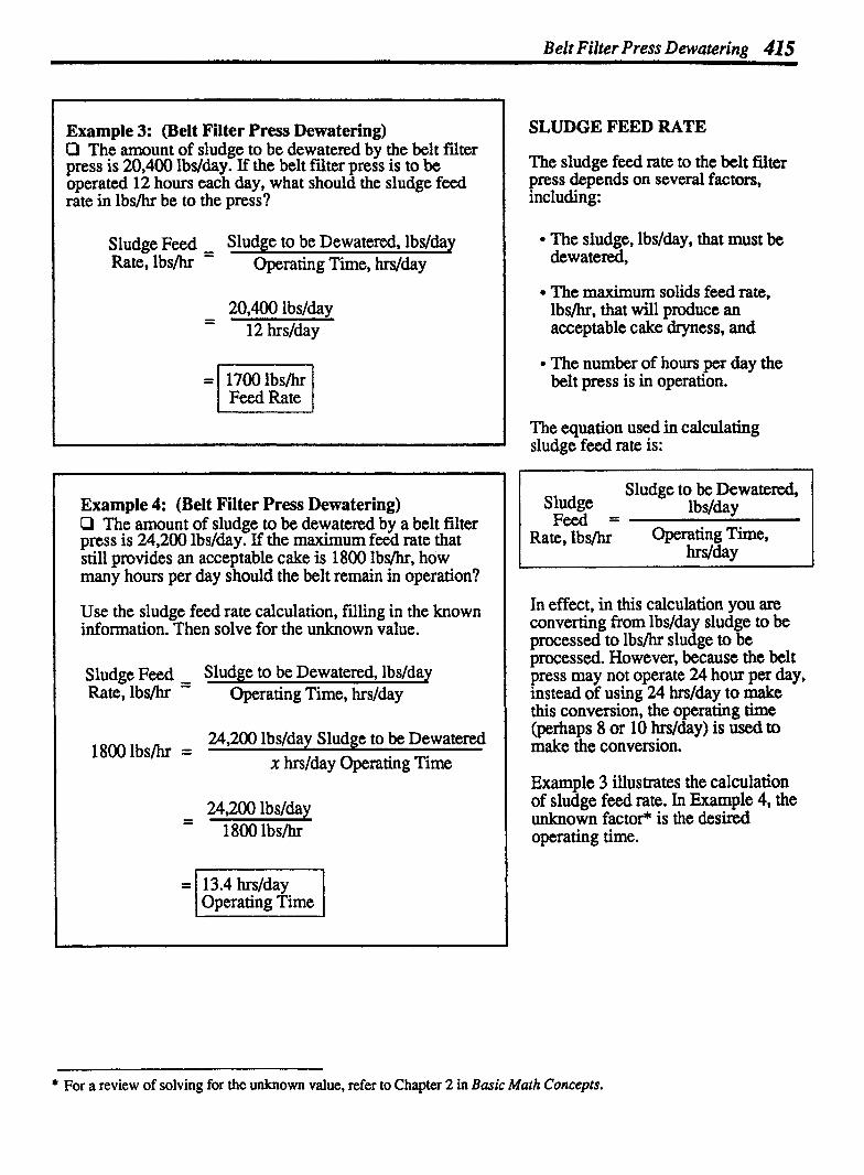
Belt Filter Press Dewatering 415
Example 3: (Belt Filter Press Dewatering) Q The amount of sludge to be dewatered by the belt filter press is 20,400 lbsfday. If the belt Nter press is to be bperated 12 hours each day, what should the sludge feed rate in lbs/h. be to the press?
Sludge Feed - Sludge to be Dewatered, lbs/da~ Rate, lbs/hr - Operating Time, hrslday
20,400 lbslday - 12 hrslday
Example 4: (Belt Filter Press Dewatering) C2 The amount of sludge to be dewatered by a belt filter press is 24,200 lbslday. If the maximum feed rate that still provides an acceptable cake is 1800 lbshr, how many hours per day should the belt remain in operation?
Use the sludge feed rate calculation, filling in the known information. Then solve for the unknown value.
Sludge Feed - Sludge to be Dewatered, lbslday Rate, lbs/hr - Operating Time, hrslday
24,200 lbs/day Sludge to be Dewatered lbs/hr =
X hrs/day Operating Time
- 24,200 lbslday - 1800 lbslhr
SLUDGE FEED RATE
=
The sludge feed rate to the belt filter press depends on several factors, including:
13.4 hrs/day Operating Time
The sludge, lbslday, that must be dew atered,
The maximum solids feed rate, lbs/hr, that will produce an acceptable cake dryness, and
The number of hours per day the belt press is in operation.
The equation used in calculating sludge feed rate is:
Sludge to be Dewatered, Sludge l b s/da y Feed =
Rate, lbs/hr Operating Time, hrslday
In effect, in this calculation you are converting from lbs/day sludge to be processed to lbs/hr sludge to be processed. However, because the belt press may not operate 24 hour per day, instead of using 24 hrslday to make this conversion, the operating time (perhaps 8 or 10 hrslday) is used to make the conversion.
Example 3 illustrates the calculation of sludge feed rate. In Example 4, the unknown factofl is the desired operating time.
* For a review of solving for the unknown value, refer to Chapter 2 in Basic Math Concepts.

41 6 Chapter 17 SLUDGE DEWATERNG AND DISPOSAL
SOLIDS LOADING RATE
The solids loading rate may be expressed as lbs/hr or as tons/hr, as desired. In either case, the calculation is based on sludge flow (or feed) to the belt press and percent or mglL concentration of total suspended solids (TSS) in the sludge.
SOL (Slud.) (60 - min) (8.34) (% TSS) LOad*=Fed, hr lbslgal 100 Rate, gpm l b s h
If the TSS infoxmation is given as mglL, the lbslday solids loading rate can be calculated as a mg/L to lbs/day problem, as shown below. By dividing by 24 hours/day, the lbslday solids loading is converted from lbslday to lbs/hr solids loading:
Solids (m&$) (MGD) (8.34 - lbs) Load. TSS Sludge Rate, = Feed
gal
l b s h 24 hrslday
To express the solids loading rate as tons/hr, simply convert lbslhr (as calculated using the equation above) to ton& solids loading rate:
Sol. Load. Rate,
tonsh
(Slud.) (60 min) (8.34) (% TS S) - F&, h, lbslgal I
= gpm 2000 lbs/ton
- - l
Example 5: (Belt Filter Press Dewatering) D The sludge feed to a belt filter press is 130 m. If the total suspended solids concentration of the fee is 4%, what is the solids loading rate, in lbs/hr?
F' Since TSS concentration is expressed as a percent, the equation using percents will be used:
Solids Loading = (Sludge) (60 min) (8.34 lbs)(% TSS) Rate, lbs/hr Feed hr gal 100
= (130 gpm) (60 min) (8.34 lbs)( 4 ) hr gal 100
I Solids Loading Rate ]
Example 6: (Belt Filter Press Dewatering) P The sludge feed to a belt filter press is 150 gpm, If the total suspended solids concentration of the feed is 45,000 mglL, what is the lbslhr solids loading rate on the belt filter press?
Since TSS concentration is expressed as mglL in this problem, the equation using mglL will be used:
(mg/L) (MGD) (8.34 lbs) TSS Sludge
Solids Loading = Feed gal
- - - -
Rate, lbslhr - 24 hrs/day
Note that the feed rate, 150 gpm, must be expressed in terms of MGD*: (1 50 gpm)(1440 midday) = 0.2 6 MGD
1 , ~ , 0 0 0
Solids Loading = (45,000 mglL) (0.2 16 MGD) (8.34 lbslgal) Rate, lbs/hr 24 hrslday
= I 3378 lbs/hr Solids Loading Rate
* Refer to Chapter 8 in Basic Mach Concepts for a review of flow conversions.
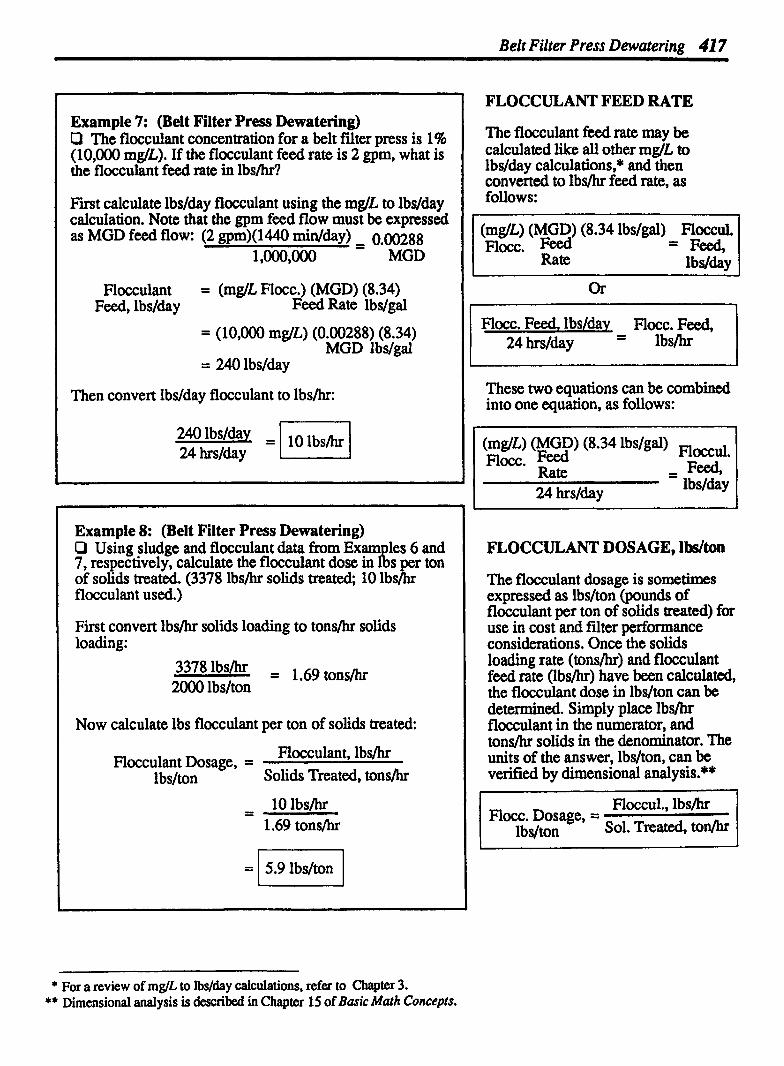
Belt Filter Press Dewaterina 41 7
Example 7: (Belt Filter Press Dewatering) P The flocculant concentration for a belt fdter prcss is 1% (10,000 mglL). If the flocculant feed rate is 2 gpm, what is the flocculant feed rate in lbs~hr?
First calculate lbslday flocculant using the mg/L to lbs/&y calculation. Note that the gpm feed flow must be expressed as MGD feed flow: (2 gpm)(1440 midday) 0.00288
l , ~ , ~ - MGD
Flocculant = (mglL Flocc.) (MGD) (8.34) Feed, lbslday Feed Rate lbslgal
= (l0,OOO mglL) (0.00288) (8.34) MGD Ibslgal
= 240 lbs/&y
Then convert lbslday flocculant to lbsb:
Example 8: (Belt Filter Press Dewatering) P Using sludge and flocculant data from Exam les 6 and it 7, respectively, calculate the flocculant dose in S per ton of solids treated. (3378 lbs/hr solids treated; 10 lbs/hr flocculant used.)
First convert lbs/hr solids loading to tons/hr solids loading:
3378 lbs* = 1.69 tons/hr 2000 lbslton
Now calculate lbs flocculant per ton of solids treated:
Flocculant Dosage, = Flocculant, l b s b
lbslton Solids Treated, tons/hr
FLOCCULANT FEED RATE
The flocculant feed rate may be calculated like a l l other mglL to l bs/day calculations,* and then converted to lbs/hr feed rate, as follows:
(mg/L) (MGD) (8.34 lbslgal) Floccul. Flocc. Feed = Feed,
Rate Wday
Flocc. Feed, lbsldq Flocc. Feed, 24 hrslday = lbslhr
These two equations can be combined into one equation, as follows:
Flocc. Rate
FLOCCULANT DOSAGE, Ibdton
The flocculant dosage is sometimes expressed as lbslton (pounds of fldcculant per ton of iolids treated) for use in cost and filter performance consi&rations. Once the solids loading rate (tons/hr) and flocculant feed rate (lbs/hr) have been calculated, the flocculant dose in lbslton can be determined. Simply place lbs/hr flocculant in the numerator, and ton* solids in the denominator. The units of the answer, lbslton, can be verified by dimensional analysis. * *
Floccul., lbslhr Flocc. Dosage, =
lbdton Sol. Treated, ton/hr
* For a review of mglL to lbs/day calculations, refer to Chapter 3. ** Dimensional analysis is described in Chapter 15 of Bacic Math Concepts.
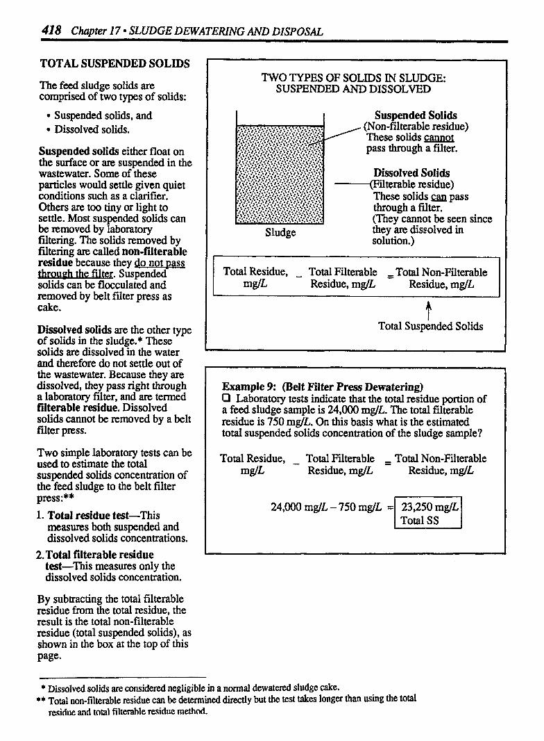
418 Chapter 17 SLUDGE DEWATERING AND DISPOSAL
TOTAL SUSPENDED SOLIDS
The feed sludge solids are comprised of two types of solids:
Suspended solids, and Dissolved solids.
Suspended solids either float on the surface or are suspended in the wastewater. Some of these particles would settle given quiet conditions such as a clarifier. Others are too tiny or light to settle. Most suspended solids can be removed by laboratory filtering. The solids removed by filtering are called non-filterable residue because they do not Dass through the filter. Suspended solids can be flocculated and removed by belt filter press as cake.
Dissolved solids are the other type of solids in the sludge.* These solids are dissolved in the water and therefore do not settle out of the wastewater. Because they are dissolved, they pass right through a laboratory filter, and are termed filterable residue. Dissolved solids cannot be removed by a belt fiter press.
Two simple laboratory tests can be used to estimate the total suspended solids concentration of the feed sludge to the belt filter press:**
1. Total residue test-This measms both suspended and dissolved solids concentrations.
2.Total filterable residue test-This measures only the dissolved solids concentration.
By subtracting the total filterable residue from the total residue, the result is the total non-filterable residue (total suspended solids), as shown in the box at the top of this Page-
TWO TYPES OF SOLIDS IN SLUDGE: SUSPENDED AND DISSOLVED
I I Suspended Solids
Sludge
on-filterable residue) These solids cannot pass through a filter.
Dissolved Solids -(Filterable residue)
These solids pass through a filter. (They cannot be seen they are dissolved in solution. )
since
Total Residue, - Total Filterable , Total Non-Filterable m@ Residue, m& Residue, mglL
A
Total Suspended Solids
Example 9: (Be1 t Filter Press Dewatering) D Laboratory tests indicate that the total residue portion of a feed sludge sample is 24,000 mglL. The total filterable residue is 750 mg/L. On this basis what is the estimated total suspended solids concentration of the sludge sample?
Total Residue, - Total Filterable - - Total Non-Filterable mdL Residue, mg/L Residue, mg/L
* Dissolved solids are considered negligible in a normal dewatered sludge cake. ** Total non-filterable residue can be determined directly but the test takes longer than using the total
residile and total filterable residue method.
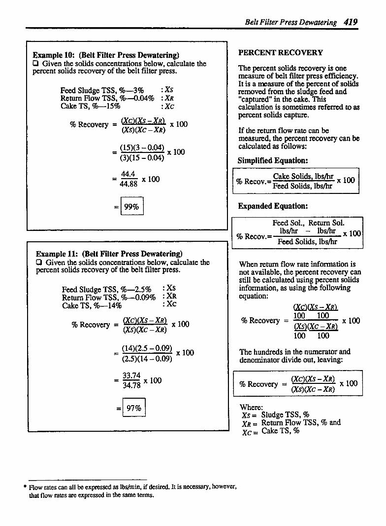
Belt Filter Press Dewaterinn 419
Example 10: (Be1 t Filter Press Dewa tering) Cl Given the solids concentrations below, calculate the percent solids recovery of the belt fdter press.
Feed Sludge TSS, 7-346 : XS Return Flow TSS, %-0.04% : XR Cake TS, 70-15% : XC
% Recovery = (Xc'CYs - X 100 (Xs)(Xc - XR)
PERCENT RECOVERY
The percent solids recovery is one measure of belt filter press efficiency. It is a measure of the percent of solids removed from the sludge feed and "captured" in the cake. This calculation is sometimes referred to as percent solids capture.
If the return flow rate can be measund, the percent recovery can be calculated as follows:
Simplified Equation:
= - 44*4 X loo 44.88
Cake Solids, lbs/hr % Recov.= Feed Solids, lbs/hr
Expanded Equation:
Example 11: (Belt Filter Press Dewatering) O Given the solids concentrations below, calculate the percent solids recovery of the belt filter press.
Feed Sludge TSS, 9s-2.5% : xs Return Flow TSS, Sb--0.09% : XR Cake TS, 40-14% : Xc
Xc)(Xs - XR) % Recovery = l (Xs)(Xc - XR)
I When return flow rate information is not available, the percent recovery can still be calculated using percent solids information, as using the following equation:
% Recovery = loo loo x100 (Xs)(Xc - XR)
The hundreds in the numerator and denominator divide out, leaving:
I Xc)(Xs - XR) % Recovery = I (Xs)(Xc - XR)
Where: Xs = Sludge TSS, % XR = Return Flow TSS, % and xc = Cake TS, %
* Flow rates can all be expressed as lbslmin. if desired. It is necessary, however, that flow rates are expressed in the same terms.
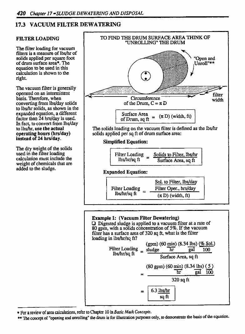
420 ChaDter 17 SLUDGE DEWATERING AND DISPOSAL
17.3 VACUUM FILTER DEWATERING
FILTER LOADING
The filter loading for vacuum filters is a measure of lbs/hr of solids applied per square foot of drum surface area*. The equation to be used in this calculation is shown to the right.
The vacuum frlter is generally operated on an intermittent basis. Therefore, when converting from lbslday solids to lbslhr solids, as shown in the expanded equation, a different factor than 24 hrslday is used. In fact, to convert from lbs/day to lbs/hr, use the actual operating hours (hrslday) instead of 24 hrdday.
The dry weight of the solids used in the filter loading calculation must include the weight of chemicals that are added to the sludge.
TO FIND THE DRUM SURFACE AREA THINK OF "UNROLLING" THE DRUM
Circumference width of the Drum, C = n: D
/ Surface Area - (n D) (width, ft) / of Drum, sq ft - The solids loading on the vacuum filter is defined as the lbs/hr solids applied per sq ft of drum surface area:
Simplified Equation:
Filter Loading Solids to Filter, l b s h lbs/hr/sq ft - Surface Area, sq ft
Expanded Equation:
1 Sol. to Filter, lbs/day I Filter Loading - Filter Oper., hrslday / lbs/hr/sqfi (n D) (width, ft)
Example 1: (Vacuum Filter Dewatering) P Digested sludge is applied to a vacuum filter at a rate of 80 gpm, with a solids concentration of 5%. If the vacuum filer has a surface area of 320 sq ft, what is the Nter loading in lbs/hr/sq ft?
Filter Loading lbs/hr/sq ft
(gpm) (60 min) (8.34 lbs) (% Sol.) - - sludge hr ad 100
Surface Area, sq ft
(80 gpm) (60 min) - (8.34 lbs) ( 5 ) - - hr 3 30
* For a review of area calculations, refer to Chapter 10 in Basic Math Concepts. ** The concept of "opening and unrolling" the drum is for illustration purposes only, U, demonstrate the basis of the equation.
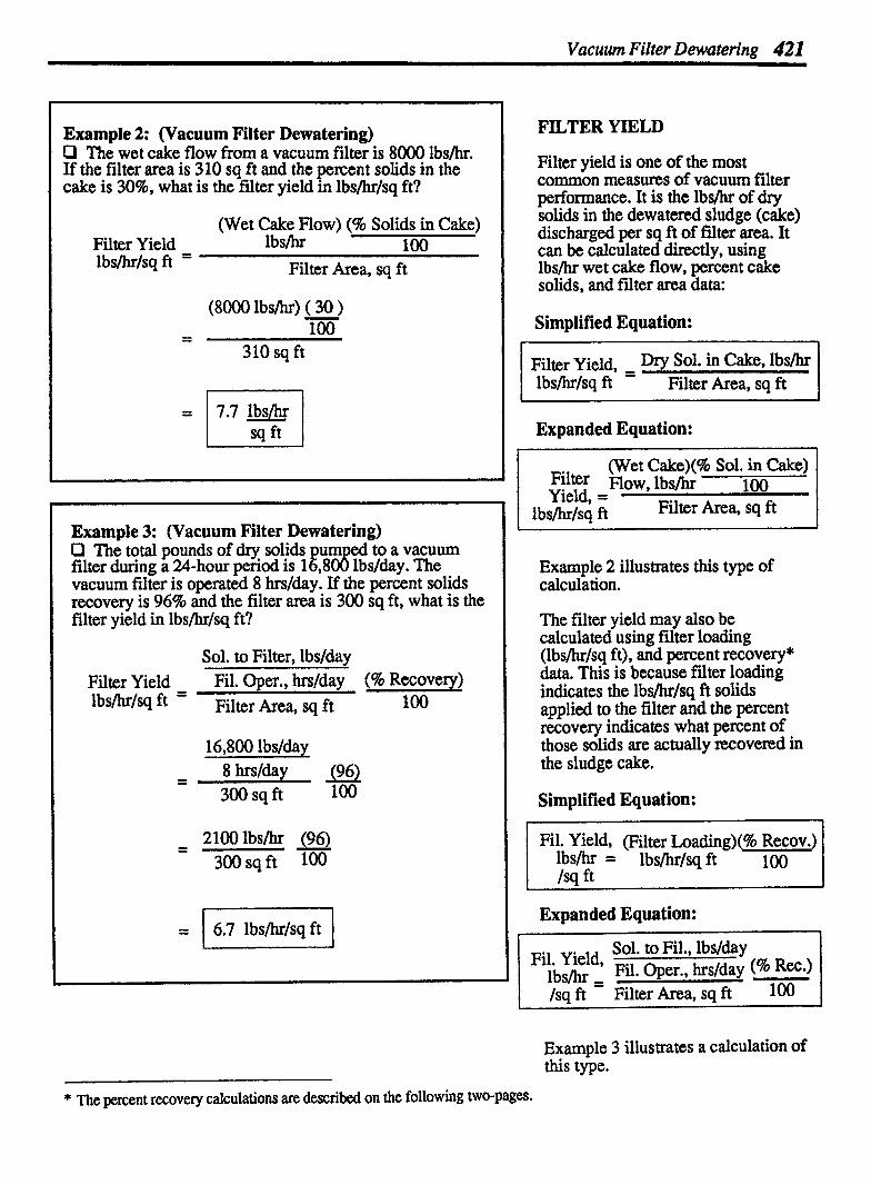
Vacuum Filter Dewatering 421
Example 2: (Vacuum Filter Dewatering) Q The wet cake flow from a vacuum filter is 8000 lbs/hr. If the filter area is 310 sq ft and the percent solids in the cake is 30%, what is the filter yield in lbs/hr/sq ft?
(Wet Cake Flow) (96 Solids in Cake) Filter Yield lbshr 100 lbs/hr/sq ft = Filter Area, sq ft
(8000 lbshr) ( 30 ) - 100
Example 3: (Vacuum Filter Dewatering) O The total pounds of dry solids urn to a vacuum ,:P filter during a 24-hour period is 1 ,8 lbslday. The vacuum filter is operated 8 hrdday. If the percent solids recovery is 9696 and the filter area is 300 sq ft, what is the filter yield in lbs/hr/sq ft?
Sol. to Filter, lbdday Filter Yield - Fil. Oper., hrs/day (96 Recovery) lbs/hr/SCl ft - Filter Area, sq ft 100
- - 21001bs/hr (96) 300 sqft 100
FILTER YIELD
Filter yield is one of the most common measures of vacuum filter performance. It is the lbs/hr of dry solids in the dewatered sludge (cake) discharged per sq ft of filter area. It can be calculated directly, using lbs/hr wet cake flow, percent cake solids, and fdter area data:
Simplified Equation:
Expanded Equation:
(Wet Cake)(% Sol. in Cake) Filter Flow, lbs/hr 100 Yield, =
lbshrlsq ft Filter Area, sq ft
Example 2 illustrates this type of calculation.
The filter yield may also be calculated using filter loading (lbslhrfsq ft), and percent recovery* data. This is because fdter loading indicates the lbs/hr/sq ft solids applied to the filter and the percent recovery indicates what percent of those solids are actually recovered in the sludge cake.
Simplified Equation:
Fil. Yield, (Filter Loading) (W l b s b = lbs/hr/sq ft 100 Isa ft
Expanded Equation: t 1
Fil. Yield, Sol. to Fil., lbs/day
lbslhr = Fil. Oper., hrs/day (% Rec.1 /sa ft Filter Area, sq ft 100
Example 3 illustrates a calculation of this type.
* The percent recovery calculations are described on the following two-pages.

422 Chapter 17 SLUDGE DEWATERING AND DISPOSAL
FILTER OPERATING TIME
The filter operating time required to process a given lbs/day solids can be calculated using the filter yield equation described on the previous page. Simply fi l l out the equation with the given data, leaving filter operation, hrs/day, as the unknown factor.* Examples 4 and 5 illustrate this calculation.
--p
Example 4: (Vacuum Filter Dewatering) Cl A total of 5000 lbslda primary sludge solids are to be fi processed by a vacuum ter. The vacuum filter yield is 2.1 lbs/hr/sq ft. The solids recovery is 96%. If the area of the filter is 200 sq ft, how many hours per day must the vacuum filter remain in operation to process these solids?
Sol. to Filter, lbslday Filter Yield Fil. Oper., hrslday (% Recovery) l b s m k ft = Filter Area, sq ft 100
5000 lbslday
2.1 lbs/hr/sq ft = X hrslday Oper. (96) 200 sq ft 100
Example 5: (Vacuum Filter Dewatering) O The total prim sludge solids to be processed b a % l' vacuum filter is 42 lbs/day. The vacuum filter yie d is 1.8 lbs/hr/sq ft. The solids recovery is 92%. If the area of the filter is 250 sq ft, how many hours per day must the vacuum filter remain in operation to process the primary sludge?
Sol. to Filter. lbs/dav Filter Yield ~ i c @er., hrdday (96 R ~ o v e r ~ ) lbsm/~q fi = Filter Area, sq ft 100
4200 lbslday
1.8 lbs~hrlsq ft = X hrslday Oper. (92) 250sqft 100
* For a review of solving for the unknown value, refer to Chapter 2 in Basic Math Concepts.

Vacuum Filter Dewaterina 423
Example 6: (Vacuum Filter Dewatering) Q The sludge feed to a vacuum filter is 3540 lbs/hr, with a solids content of S S % , If the wet cake flow is 625 lbs/hr with a 30% solids content, what is the percent solids recovery?
(Wet Cake Flow)(% Solids in Cake) % Solids - lbs/hr 100 Recovery - (Sludge Feed)(% Sol. in Feed)
X 100
- - loo X loo (3540 lbs/hr) ( 5.5 )
100
= 96% Solids I Recovery 1
Example 7: (Vacuum Filter Dewatering) P The sludge feed to a vacuum filter is 98,000 lbs/day, with a solids content of 6%. If the wet cake flow is 19,500 lbs/day, with a 28% solids content, what is the percent solids recovery?
Wet Cake Flow)(% Solids in Cake) . , . % Solids
,
- l bs/day 100 Recovery - (Sludge Feed)(% Sol. in Feed) X 100
(19,500 lbs/day)( 28 ) - - loo X loo
(98,000 lbs/day) ( 6 )
= 93%Solids I Recovery / * Note that the 100 in the numerator and denominator of the fraction can be
divided out. However the 100 shown to the right must not be cancelled. * * Operations Manual4ludge Handling and Conditioning. EPA. 1978.
PERCENT SOLIDS RECOVERY
The function of the vacuum filtration process is to separate the solids fiom the liquids in the sludge being processed. Therefore, the efficiency of the process is the percent of feed solids "recovered in the filter cake. This is sometimes referred to as the percent solids capture.
Simplified Equation:
% Sofia - Sol. in Cake, lbs/hr Recovery - Sol. in Feed, lbs/hr I Expanded Equation:*
(Wet Cake) (46 Sol. in Cake) 4% Sol,Flow, lbs/hr loo X loo Rec* - (Sl. Feed) (% Sol. in Feed)
When the wet cake flow rate is not known, another equation may be used This equation uses only suspended solids data to determine solids recovery:**
(Cake) (Feed - Filtrate) I % Sol.,% sol.,% Sol.,% 100 1
Recov ' (Feed) (Cake - Fil.)
If chemicals are added to the vacuum filter, filtrate solids must be corrected as shown below. This is because the filtrate has been diluted by additional water from the chemical and dilution water feeds. The measured filtrate solids, are actually less than they would have been had the additional water not been added.
First calculate the correction factor:
(Feed rate)+(Chem. Flow)+@ilution) lbdhr lbs/hr Wat., lbs/hr
Feed Rate, lbs/hr
Then multiply the measured fdtrate solids by the correction factor:
Corrected , (Meas. Filtrate) (Con.) Filtrate Sol. Solids Factor

424 Chapter 17 SLUDGE DEWATERING AND DISPOSAL
17.4 SAND DRYING BEDS CALCULATIONS
TOTAL SLUDGE APPLIED
The total gallons of sludge applied to sand drying beds may be calculated using the dimensions of the bed and depth of sludge applied, as shown in the diagram to the right.*
GALLONS DRYING BED VOLUME
J.
/-l - width, ft
Volume, = (len th) (width) (de th) (7.48 gal) ft 8 cu ft
Example 1: (Sand Drying Beds) Q A drying bed is 225 ft long and 25 ft wide. If slud e is
are applied to the drying bed? H applied to a depth of 4 inches, how many gallons of S udge
Volume, , gal
(1) (W) ( a (7.48 m cu ft
= (225 ft) (25 ft) (0.33 ft) (7.48 gal) cu ft
= 1 13,885 gal 1
* For a review of volume calculations, refer to Chapter 11 in Basic Math Concepts.

Sand Dryinn Beds 425
Example 2: (Sand Drying Beds) D A sludge bed is 200 ft lon and 20 ft wide. A total of
fi 17 1,600 lbs of sludge are app ed each application of the sand drying bed. The sludge has a solids content of 5%. If the drying and removal cycle requires 21 days, what is the solids loading rate in lbs/yr/sq ft?
Solids (Sludge Applied, lbs) (365 -- days) (96 Sol.) Loading - - Days of Applic. Yr 100 Rate, Bed Area, sq ft
lbs/yr/sq ft (171,600 lbs) (365 days) ( 5 ) - -
- - 21 days Yr 100 (200 ft)(20 ft)
Example 3: (Sand Drying Beds) C3 A sludge drying bed is 180 ft long and 25 ft wide. The sludge is applied to a depth of 8 inches. The solids concentration of the sludge is 4.5%. If the drying and removal cycle requires 18 days, what is the solids loading rate to the beds in lbs/yr/sq ft?
First calculate the lbs of sludge applied: (8 in. = 0.67 ft)
(180 ft) (25 ft) (0.67 ft) (7.48 - gal) ( 8 . 3 4 5 = 188,085 cu ft gal
Then determine the solids loading rate:
I lbs I Solids (1 88,085 lbs) (365 days) ( 4.5 ) -
Loading - 18 days 100 Rate, -
lbslyrlsq ft (180 ft)(25 ft)
SOLIDS LOADING RATE
The sludge loading rate may be expressed as lbdyrlsq ft. This loading rate is dependent on:
Sludge applied per application, lbs,
Percent solids concentration,
Cycle length, and
Square feet of sand bed area.
The equation for sludge loading rate is given below.
Simplified Equation:
Solids Loading -
Rate, - lbs/yr/sq ft
(Sludge Applied,) (% Sol.) lbslyr 100 Bed Area, sq ft
Expanded Equation:
Solids Loading
Rate, = lbslyrlsq ft
lbs Sludge I plied (365) (% Sol.)
Days of da~s/yr 100
(length, ft) (width,ft)
Note that the first term in the numerator of the expanded equation is simply lbslday sludge:
lbs Sludge , - lbs Sludge Days of Applic day
The lbslday sludge is then multiplied by 365 days per year and percent solids.
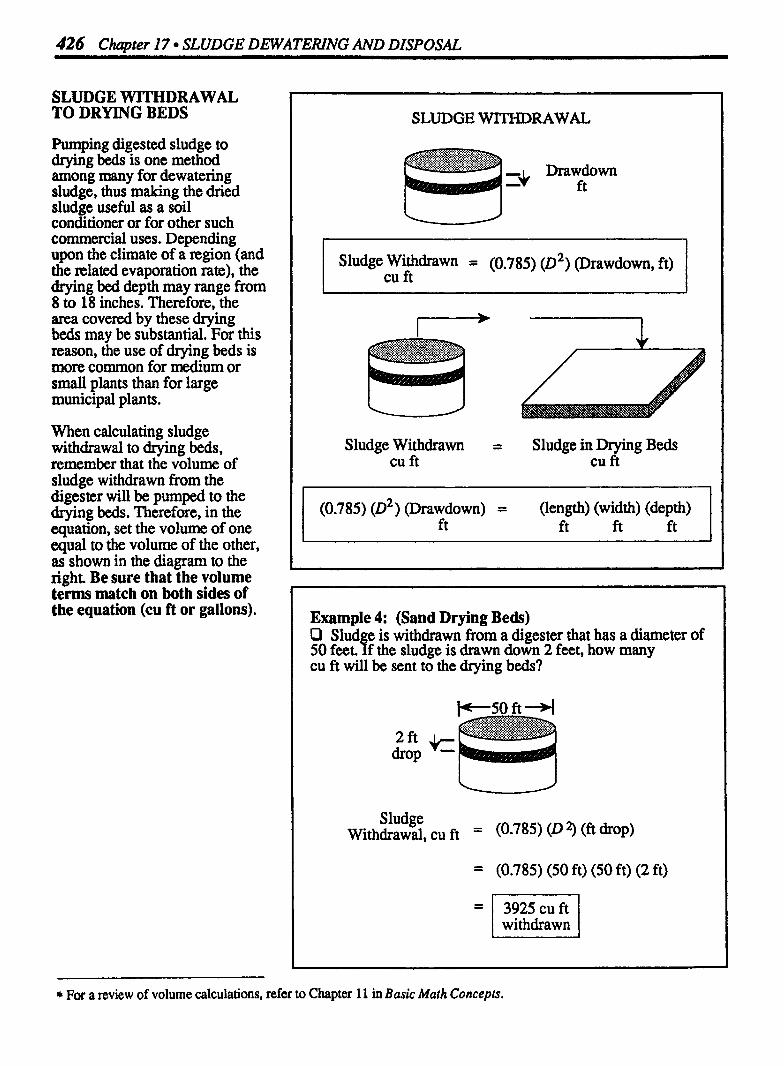
426 Chapter I7 SLUDGE DEWATERING AND DISPOSAL
SLUDGE WITHDRAWAL TO DRYING BEDS
Pumping digested sludge to drying beds is one method among many for dewatering sludge, thus making the dried sludge useful as a soil conditioner or for other such commercial uses. Depending upon the climate of a region (and the dated evaporation rate), the drying bed depth may range from 8 to 18 inches. Therefore, the area covered by these drying beds may be substantial. For this reason, the use of drying beds is more common for medium or small plants than for large municipal plants.
When calculating sludge withdrawal to drying beds, remember that the volume of sludge withdrawn from the digester will be pumped to the drying beds. Therefore, in the equation, set the volume of one equal to the volume of the other, as shown in the diagram to the right. Be sure that the volume terms match on both sides of the equation (cu ft or gallons).
SLUDGE WITHDRAWAL
sludge l W & ~ n = (0.785) (02) (Drawdown, ft) cu ft
Sludge Withdrawn = Sludge in Drying Beds cu ft cu ft
(0.785) (02) (Drawdown) = (length) (width) (depth) ft ft ft ft
Example 4: (Sand Drying Beds) O Slud e is withdrawn fiom a digester that has a diameter of 50 feet f the sludge is drawn down 2 feet, how many cu ft will be sent to the drying beds?
2ft * drop -
Sludge - (0.785) (D z) (ft drop) Withdrawal, cu ft - = (0.785) (50 ft) (Soft) (2ft)
= 1 3925 cu ft / withdrawn
* For a review of volume calculations, refer to Chapter 11 in Basic Math Concepts.
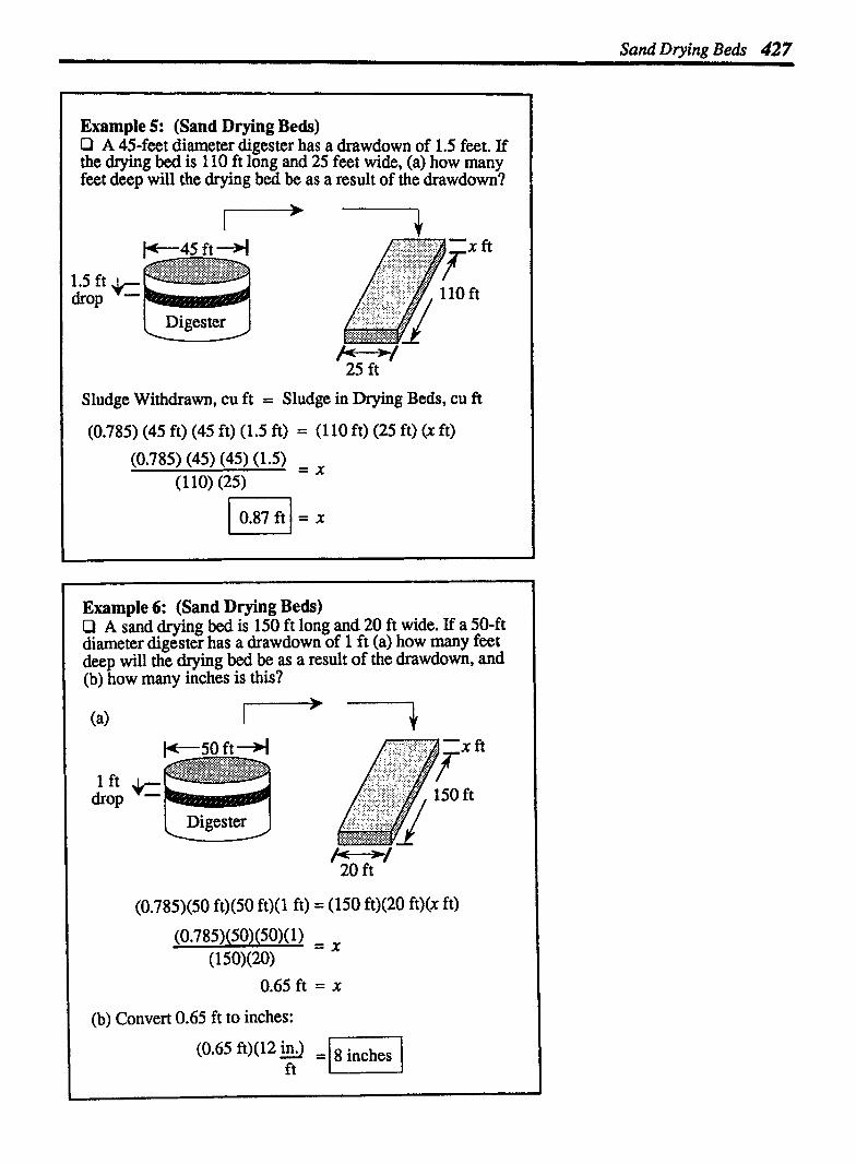
Sand Drvinn Be& 427
Example S: (Sand Drying Beds) O A 45-feet diameter digester has a drawdown of 1.5 feet. If the drying bed is l l0 ft long and 25 feet wide, (a) how many feet deep will the drying bed be as a result of the drawdown?
1.5 ft +- drop -
Sludge Withdrawn, cu ft = Sludge in Drying Beds, cu ft
(0.785) (45 ft) (45 ft) (1.5 ft) = (1 10 ft) (25 ft) (X ft)
Example 6: (Sand Drying Beds) O A sand drying bed is 150 ft long and 20 ft wide. If a 50-ft diameter digester has a drawdown of 1 ft (a) how many feet deep will the drying bed be as a result of the drawdown, and (b) how many inches is this?
l f t +- drop -
(0.785)(50 ft)(50 ft)(l ft) = (150 ft)(20 ft)(x ft)
(b) Convert 0.65 ft to inches:
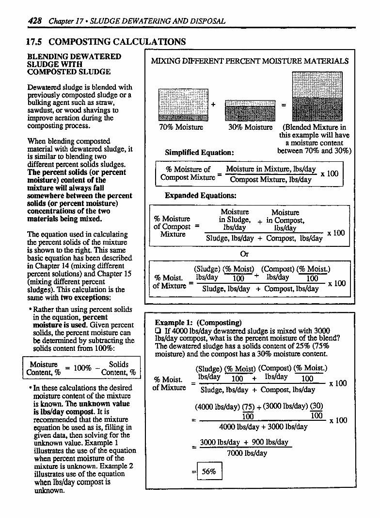
428 Chapter 17 SLUDGE DEWATERING AND DISPOSAL
17.5 COMPOSTING CALCULATIONS
BLENDING DEWATERED SLUDGE WITH COMPOSTED SLUDGE
Dewatered sludge is blended with previously composted sludge or a bulking agent such as straw, sawdust, or wood shavings to improve aeration during the cornposting process.
When blending composted material with dewatered sludge, it is similar to blending two different percent solids sludges. The percent solids (or percent moisture) content of the mixture will always fall somewhere between the percent solids (or percent moisture) concentrations of the two materials being mixed.
The equation used in calculating the percent solids of the mixture is shown to the right. This same basic equation has been described in Chapter 14 (mixing different percent solutions) and Chapter 15 (mixing different percent sludges). This calculation is the same with two exceptions:
Rather than using percent solids in the equation, percent moisture is used. Given percent solids, the percent moisture can be determined by subtracting the solids content from 100%:
Moisture Solids Content, 96 = '00% -content, %
In these calculations the desired moisture content of the mixture is known. The unknown value is lbdday compost. It is recommended that the mixture equation be used as is, filling in given data, then solving for the unknown value. Example 1 illustrates the use of the equation when percent moisture of the mixture is unknown. Example 2 illustrates use of the equation when lbslday compost is unknown.
MIXING DIFFERENT PERCENT MOISTURE MATERIALS
70% Moisture 30% Moisture (Blended Mixture in this example will have
a moisture content Simplified Equation: between 70% and 30%)
96 Moisture of Moisture in Mixture, lbsjday Compost Mixture ' Compost Mixture, lbsjday
Expanded Equations:
Moisture Moisture % Moisture in Sludge, + in Compost, of Compost = l bs/day l bs/da
Mixture Sludge, lbs/day + Compos: lbslday X 100
(Sludge) (% Moist) (Compost) (% Moist) % Moist. Wday 1 0 + lbdday
loo xloo of Mixture = Sludge, lbs/day + Compost, lbslday
Example 1: (Composting) P If 4000 lbslday dewatered sludge is mixed with 3000 lbdday compost, what is the percent moisture of the blend? The dewatered sludge has a solids content of 25% (75% moisture) and the compost has a 30% moisture content.
% Moist. - - Wday 100 + WdaY 100 of Mixture Sludge, lbslday + Compost, lbslday
(4000 lbslday) (75) + (3000 lbslday) (30) - - 100
4000 lbslday + 3000 lbslday loo X loo
- - 3000 lbslday + 900 lbslday 7000 lbsjday

Example 2: (Composting) O A treatment plant produces a total of 5500 lbslday of dewatered digested primary sludge. The dewatered sludge has a solids concentration of 28%. Final compost to be used in blending has a moisture content of 32%. How much compost (lbslday) must be blended with the dewatered sludge to produce a mixture with a moisture content of SO%?
The dewatered sludge has a solids content of 28%; therefore the moisture content is 72%.
(Sludge) (% Moist) (Compost) (96 Moist.) % Moist. - lbS/dBy 100 + W&Y 100 X of Mixture - Sludge , lbslday + Compost, lbs/day
First, move the 100 to the left side of the equation; then simplify terms before rearranging to solve for X*:
50 3960 lbslday + (X lbs/day)(0.32) m0 = 5500 lbslday + x lbs/day
Next, group X terns on the left side of the equation, and numbers on the right side:
X = 1 67221bslday I Compost Req'd
* For a review of solving for the unknown value, refer to Chapter 2 in Basic Math Concepts.

430 Chapter 17 SLUDGE DEWATERINC AND DISPOSAL
BLENDING DEWATERED SLUDGE WITH WOOD CHIPS
When blending dew atered sludge and wood chips, the same basic "mixing equation" may be used. The basis of the percent solids calculation is simply the pounds of solids in the blended compost divided by the total pounds of blended compost, as shown by the simplified equa- tion. The expanded equations are merely refinements of this basic concept.
The first expanded equation identifies the two sources of materials to be blended. Solids from the sludge and solids from the wood chips (numerator) constitute the solids in the blended product. The total pounds of compost blend is comprised of the pounds of sludge and the pounds of wood chips (denominator).
Since the sludge and compost is often mixed on the basis of volumes (cubic yards), the second expanded equation gives each component in terns of cubic yards. Then, because percent solids calculations should be made on the basis of weight, a lbs/cu yd factor must accompany each quantity of cubic yards. In this way, each component of the blend is still represented as pounds.
The lbslcu ft density of the sludge and wood chips (bulk density) is generally given for wet sludpe and wet wood chips, and not for dry solids, as shown in the second expanded equation. Therefore, the third expanded equation includes the sludge and wood chip data with the corresponding bulk density and percent solids factors.
MIXING SLUDGE AND WOOD CHIPS
Wood Chips
+ - -
17% Solids 55% Solids (Blended compost in this example will have
a solids content between 17% and 55%)
Simplified Equation:
% Solids of - Solids in Compost Blend, lbs I - Compost Blend, ibs
Expanded Equations:
% Solids Solids in Solids in Wood of Compost = Sludge, lbs + Chips, lbs
X 100 - - - - - I Blend Sludge, lbs + Wood Chips, lbs I
% Solids of =
I
t Bulk density of
? Bulk density of
Sludge Wood Chips
I
( cu yds ) ( lbs ) ( cu yds ) ( lbs ) Solids in ,Yd + Solids in Gd Sludge Wood Chips,
.
Bulk density of Bulk density of Slufge Woof Chips
% (cu yds) ( lbs ) (% Sol.) (cu yds) ( lbs ) (% Sol.) -- - Solids Sludge yd 100 + W-c- cu yd of = loo X loo
Compost (cu yds) ( lbs ) + (cu yds) ( lbs ) - Blend sludge c u d W. c- cu yd
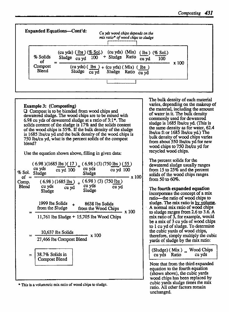
Composting 431
Expanded Equat iondont 'd: Cu ydr wood chips dependr on the -ratio* of wood chips to sludge
r----------- I 1
(CU yds) ( lbs ) (% Sol.) (cu yds) (Mix) ( lbs ) (% Sol.) % Solids Sludge cu yd 100 + Sludge Ratio Gd 100
of = Compost
X 100 (CU yds) ( lbs ) + (cu yds) ( Mix) ( lbs )
Blend - Sludge cu yd Sludge Ratio cu yd
Example 3: (Composting) Q Compost is to be blended from wood chips and dewatered sludge. The wood chips are to be mixed with 6.98 cu yds of dewatered sludge at a ratio of 3: l*. The solids content of the sludge is 17% and the solids content of the wood chips is 55%. If the bulk density of the sludge is 1685 lbs/cu yd and the bulk density of the wood chips is 750 lbslcu yd, what is the percent solids of the compost blend?
Use the equation shown above, filling in given data:
( 6.98 )(l685 lbs )( 17 ) + ( 6.98 ) (3) (750 lbs ) ( 55 ) -- - CU Y ~ S c, yd 100 CU Y ~ S cuyd 100
% sole Sludge Sludge of = X 100
cornp. ( 6.98 ) (1685 - lbs ) + ( 6-98 ) (3) (750 lbs ) Blend cu yds cu yd cu yds
Sludge c u d
Sludge
1999 lbs Solids + 8638 lbs Solids
- from the Sludge from the Wood Chips - X 100 11,761 lbs Sludge + 15,705 lbs Wood Chips
- - 10,637 lbs Solids X 100
27,466 lbs Compost Blend
* This is a volumetric mix ratio of wood chips to sludge.
=
The bulk density of each material varies, depending on the makeup of the material, including the amount of water in it. The bulk density commonly used for dewatered sludge is 1685 lbslcu yd. (This is the same density as for water, 62.4 lbs/cu ft or 1685 lbs/cu yd.) The bulk density of wood chips varies k m about 550 lbslcu yd for new wood chips to 750 lbslcu yd for recycled wood chips.
38.7% Solids in Compost Blend
The percent solids for the dewatered sludge usually ranges from 15 to 25% and the percent solids of the wood chips ranges from 50 to 60%.
The fourth expanded equation incorporates the concept of a mix ratio--the ratio of wood chips to sludge. Thc mix ratio is bv volume. A normal mix ratio of wood chips to sludge ranges from 2.6 to 3.6. A mix ratio of 3, for example, would be a mix of 3 cu yds of wood chips to 1 cu yd of sludge. To determine the cubic yards of wood chips, therefore, simply multiply the cubic yards of sludge by the mix ratio:
l (Sludge) ( Mix ) cu yds Ratio cu yds
Note that from the third expanded equation to the fourth equation (shown above), the cubic yards wood chips has been replaced by cubic yards sludge times the mix ratio. All other factors remain unchanged.

432 Chapter 17. SLUDGE DEWATERING AND DISPOSAL
COMPOST SITE CAPACITY CALCULATION
An important consideration in compost operation is the solids processing capability, lbslday or lbslwk.
This type of calculation is essentially a detention time or fill time problem*, as illustrated by the simplified equation shown to the right. Consistent with other fill time calculations, the volume is in the numerator of the equation and the fill rate is in the denominator.
The expanded equations replace wet compost, cu ydsl day with equivalent expressions. For example, in the first expanded equation, note that the denominator of the equation (wet compost, lbslday + compost bulk density, lbslcu yd) is equivalent to wet compost, cu ydslday.
There is substitution of terms in each succeedin expanded equation until lb sf day dry solids is included in the equation. This term is desirable since it is frequently the unknown variable in compost site capacity calculations.
THE SITE CAPACITY CALCULATION IS A DETENTION TIME OR "FILL TIME" CALCULATION*
cu yds available capacity Simplified Equation:
Fill Time, - Total Available Capacity, cu yds - days Wet Compost, cu yddday
Expanded Equation:
1 Fill Time, - - Total Available Capacity, cu yds I -
I days
Wet Compost, lbslday Compost Bulk Density, lbs/cu yd
Fill Time, - - Total Available Capacity, cu yds days Wet Sludge + Wet Wood Chips
lbslday l b slda y Compost Bullc Density, lbslcu yd
Fill Total Available Capacity, cu yds - - Time, - days Dry solids + @ry solids) ( Mix ) (Bulk Dens.)
l bs/day lbslday Ratio of % Sol loo
% Sol 100
Wood Chips, lbslcu yd
Slud. Bulk Dens., Ibslcu yd
Compost Bulk Density, lbslcu yd
The last equation is then rearranged as:
Fill (Avail. Capac., cu yds) (Comp. Bulk Dens., lbslcu yd)
% Sol % Sol lbslcu yd Slud. Bulk
Dens., lblcu yd
* Refer to Chapter 5 for a review of detention and retention time calculations.

Composting 433
Example 4 : (Composting) Q A composting facility has an available capacity of 7800 cu yds. If the composting cycle is 21 days, how many lbslday wet compost can be processed by this facility? Assume a compost bulk density of 1000 lbslcu yd. *
Fill Time, - - Total Available Capacity, cu yds days Wet Comwst, lbs/dw
Compost Bulk Density, lbslcu yd
7800 cu yds 21 days =
x lbs/day
21 days = (7800 cu yds) (1000 lbslcu yd)
x lbslday
x lbslday = (7800 cu yds) (1000 lbslcu yd) 21 days
Example 5 : (Composting) Cl A composting facility has an available capacity of 5500 cu yds. If the composting cycle is 21 days, how many lbslday wet compost can be processed by this facility? How many tonslday is this? Assume a compost bulk density of 950 lbslcu yd.*
5500 cu yds 21 days =
x lbslday 950 lbslcu yd
2ldays = (5500 cu yds) (950 lbslcu yd)
X lbslday
x lbslday = (5500 cu yds) (950 lbslcu yd)
21 days
The lbslday compost can now be converted to tonsiday:
* For a review of solving for the unknown value, refer to Chapter 2 in Basic Math Concepts.
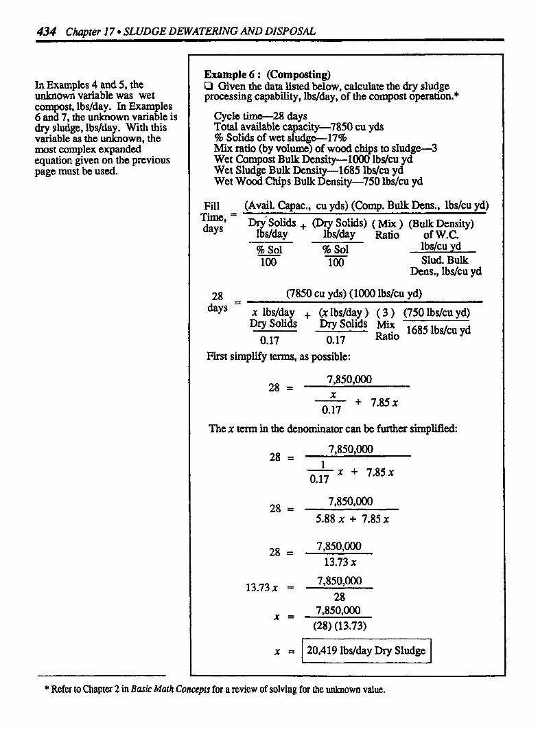
434 Chapter I7 SLUDGE DEWATERING AND DISPOSAL
In Examples 4 and 5, the unknown variable was wet compost, lbs/day . In Examples 6 and 7, the unknown variable is dry sludge, lbsfday. With this variable as the unknown, the most complex expanded equation given on the previous page must be used.
Example 6 : (Composting) 0 Given the data listed below, calculate the dry sludge processing capability, lbs/day, of the compost operation.*
Cycle thm-28 days Total available capacity-7850 cu yds % Solids of wet sludge-17% Mix ratio (by volume) of wood chips to sludge-3 Wet Compost Bulk Density-1000 lbs/cu yd Wet Sludge Bulk Density-1685 lbs/cu yd Wet Wood Chips Bulk Density-750 lbslcu yd
Fill (Avail. Capac., cu yds) (Comp. Bulk Dens., lbslcu yd)
% Sol 100
% Sol 100
lbslcu yd Slud. Bulk
Dens., lbslcu yd
7.R (7850 cu yds) (1000 lbslcu yd) dayS X lbslday + (X lbslday ) ( 3 ) (750 lbs/cu yd)
Solids Dry Solids Mix 1685 1bsfcu yd 0.17 0.17 Ratio
First simplify terms, as possible:
The x term in the denominator can be further simplified:
X = I 20,419 lbs/day Dry sludge I * Refer to Chapter 2 in Basic Marh Concepts for a review of solving for the unknown value.

Composting 435
Example 7 : (Composting) O Given the data listed below, calculate the dry sludge, lbsfday, that can be processed at the compost facility.
Cycle time-28 days Total available capacity-7850 cu yds % Solids of wet sludg+17% Mix ratio (by volume) of wood chips to sludge-3.45 Wet Compost Bulk Density-1000 lbs/cu yd Wet Sludge Bulk Density-1685 lbsfcu yd Wet Wood Chips Bulk Density-750 lbs/cu yd
Fill (Avail. Capac., cu yds) (Comp. Bulk Dens., lbs/cu yd)
% Sol % Sol 100 100
lbsfcu yd Slud. Bulk
Dens., lbsfcu yd
28 (7850 cu yds) (1000 lbslcu yd) - days x lbsfday + (X lbsfday ) (3.45) (750 lbs/cu yd)
Dry Solids - Dry Solids ~ i x Ratio 1685 lbs/cu yd 0.17 0.17
First simplify terms, as possible:
The x tern in the denominator can be further simplified
1 18,803 lbslday Dry Sludge /
* Expressed in terms of tons/day, this is 18.803 lbs/day + 2000 lbs/ton = 9.4 tons/day.
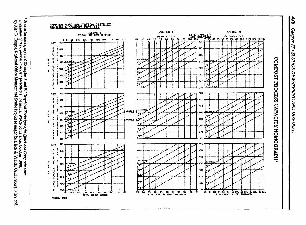
436 C
hapter 17 SLU
DG
E D
EWATERIN
G A
ND
DISPO
SAL
CO
MPO
ST PR
OC
ESS C
APA
CIT
Y N
OM
OG
RA
PH*
p-
* Source for nornograph and Exam
ples 8 and 9: "Graphical Techniques for Q
uick and Com
prehensive E
valuation of the Com
post Process," presented at the annual WPC
F conference, October, 1990,
by Alan B. C
ooper, Regional O
ffice Manager and Senior Project M
anager for Black & V
eatch, Gaithersburg, M
aryland.
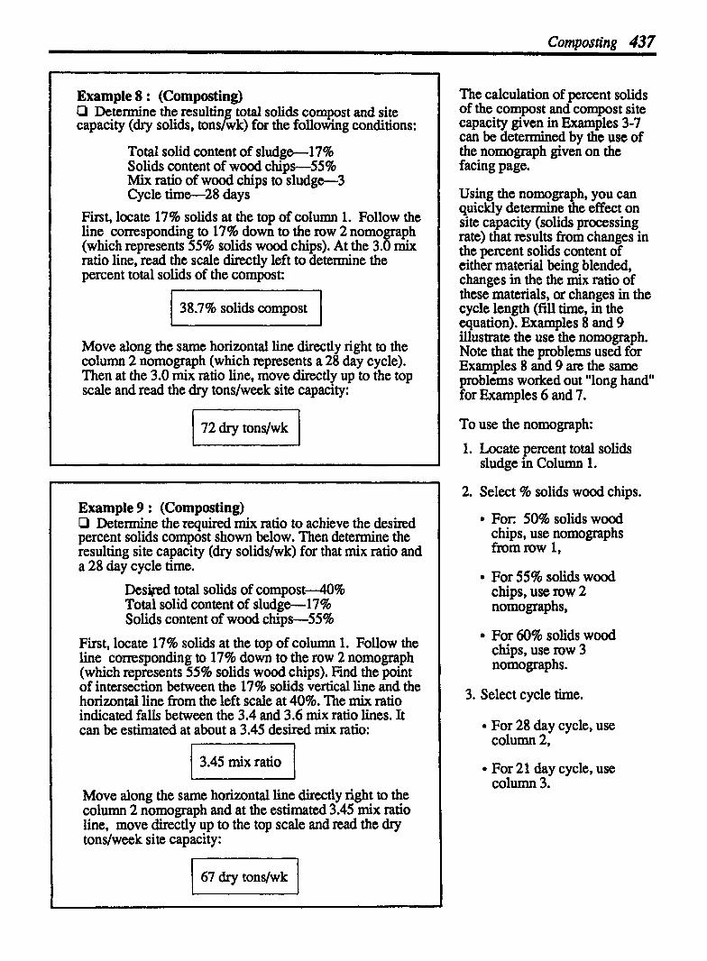
Composting 437
Example 8 : (Composting) O Determine the resultin total solids compost and site capacity (dry solids, tons B wk) for the following conditions:
Total solid content of sludgt+17% Solids content of wood chips-55% Mix ratio of wood chips to sludge-3 Cycle t i m e 2 8 days
First, locate 17% solids at the top of column 1. Follow the line comsponding to 17% down to the row 2 nomograph (which represents 55% solids wood chips). At the 3.0 mix ratio line, read the scale directly left to determine the percent total solids of the compost:
1 38.7% solids compost I Move along the same horizontal line directly right to the column 2 nomograph (which represents a 28 day cycle). Then at the 3.0 mix ratio line, move directly up to the top scale and read the dry tonslweek site capacity:
Example 9 : (Composting) P Determine the required mix ratio to achieve the desired percent solids compost shown below. Then determine the resulting site capacity (dry solidslwk) for that mix ratio and a 28 day cycle time.
Des- total solids of compos t4% Total solid content of sludg- 17% Solids content of wood chips-55%
First, locate 17% solids at the top of column 1. Follow the line corresponding to 17% down to the row 2 nomograph (which represents 55% solids wood chips). Find the point of intersection between the 17% solids vertical line and the horizontal line from the left scale at 40%. The mix ratio indicated falls between the 3.4 and 3.6 mix ratio lines. It can be estimated at about a 3.45 desired mix ratio: - 1 3.45 mix ratio I Move along the same horizontal line directly right to the column 2 nomograph and at the estimated 3.45 mix ratio line, move directly up to the top scale and read the dry tonslweek site capacity:
1 67 dry tonslwk I
The calculation of percent solids of the compost and compost site capacity given in Examples 3-7 can be determined by the use of the normgraph given on the facing page.
Using the nomograph, you can quickly determine the effect on site capacity (solids processing rate) that results from changes in the percent solids content of either material being blended, changes in the the mix ratio of these materials, or changes in the cycle length (fill time, in the equation). Examples 8 and 9 illustrate thc use the nomograph. Note that the problems used for Examples 8 and 9 are the same problems worked out "long hand for Examples 6 and 7.
To use the nornograph:
1. Locate percent total solids sludge in Column 1.
2. Select % solids wood chips.
For: 50% solids wood chips, use nornographs from row 1,
For 55% solids wood chips, use row 2 nomographs,
For 60% solids wood chips, use row 3 nomographs.
3. Select cycle time.
For 28 day cycle, use column 2,
For 21 day cycle, use column 3.


1 8 Laboratory Calculations
1. Biochemical Oxygen Demand (BOD)
Simplified Equation:
BOD DO Used During S-day Test, mglL % Dilution of Sample
Expanded Equation:
I BOD = Initial DO, mg/L DO After S-days, mg/L I Sample Volume, m1 I
I BOD Bottle Volume, m1 I
7-Day Average BOD:
BOD + BOD, BOD + BOD + BOD + BOD + BOD 7-&Y Day l Day 2 Day 3 Day 4 Day S Day 6 Day 7 A v e r -..
A = . w 1 . - - BOD

440 Chapter I8 LABORATORY CALCULATIONS
Moles
Liters Solution
Molarity = Moles Solute Liters Solution
Molarity = Grams of Chemical Formula Wt. of the Chemical
1 3. Normality and Equivalents
Normality= No. of Equivalents of Solute Liters of Solution
Equivalent - Formula Wt Weight Net Valence
4. Settleability*
% Settleable - - Settled Solids 100 2000 rnl Sample l
I * Using a Mallory Direct Reading Settleorneter.
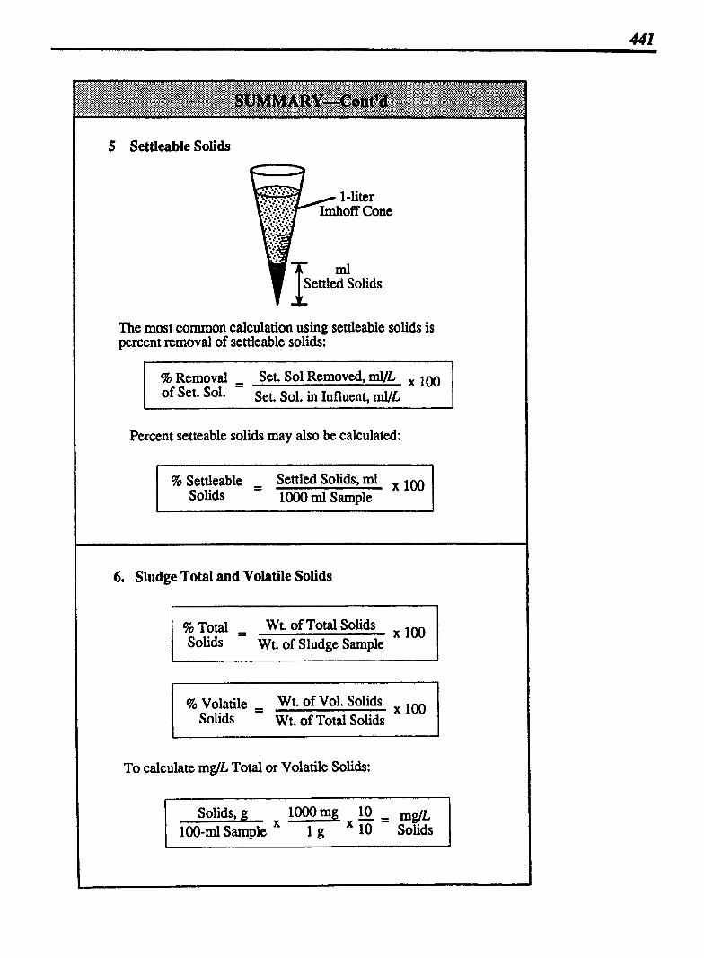
5 Settleable Solids
1 l-liter
I Settled Solids
The most common calculation using settleable solids is percent removal of settleable solids:
% Removal - Set. Sol Removed, mVL ,100 of Set* Set. Sol. in Influent, W L
Percent setteable solids may also be calculated:
% Settleable - - Settled Solids. lm l Solids lOOO m1 Sample
I 6. Sludge Total and Volatile Solids
% Total , - Wt.ofTotalSolids xlOO solids Wt. of Sludge Sample
% volatile , Wt. of Vol. Solids Solids Wt. of Total Solids
l To calculate mg/L Total or Volatile Solids:
Solids,g m g l ~ 100-m1 Sample l g Solids

442 Chapter 18 LABORATORY CALCULATIONS
7. Suspended Solids and Volatile Suspended Solids
To calculate mg/L SS, if a 25-d, sam~le is used:
To calculate mg/L SS, jf a 50-mC, S
grams SS lOOO*g x20 = mg SS = mglL 5 0 - m ~ Sample X l g 20 li ter SS
To cdcula te percent volatile suspended solids:
%VSS = Wt. of Volatile Solids
Wt. of Suspended Solids
8. Sludge Volume Index and Sludge Density Index
Density, g v SDI =
Volume, mC,

9. Temperature
Fahrenheit to Celsius : (Conventional Equation)
Celsius to Fa h renheit : (Conventional Equation)
3-Step Met hod: (Converting either direction)
1. Add 40'.
2. Multiply by 5/9 or 9/5. (Depends on the direction of conversion.)
3. Subtract 40'.
NOTES:
1

444 Chapter I8 LABORATORY CALCULATIONS
18.1 BIOCHEMICAL OXYGEN DEMAND (BOD) CALCULATIONS
The Biochemical Oxygen Demand (BOD) content of a wastewater is used as an indicator of the available food in the wastewater, and is therefore included in such calculations as organic loading and F M ratio.
The BOD test measures the amount of oxygen used by the microorganisms as they breakdown food (complex organic compounds) in the wastewater.
The dissolved oxygen (DO) content of the sample is tested just prior to beginning the test (initial DO) and at the end of the test. Then by subtracting the second DO reading from the initial DO, the amount of DO used during the test can be determined:
Initial 1 DO, m& DO After 5-day Test
mglL
DO Used = During
mglL
If the BOD test were conducted using a full-strength sample, the BOD content (mg/L) would be equal to the dissolved oxygen (DO) used or depleted during the 5-day test. For example, if the DO used during the 5-day BOD test was 75 mglL, then the BOD would be the same-75 mglL.
However, the BOD test is conducted on a diluted sample. Therefore, the percent dilution of the sample must be included in the calculation, as shown in the equations to the right.*
Depending on the percent dilution, the DO used in the diluted sample might represent only 1% to 10% of the DO used in the full-strength sample.
THE BOD TEST IS CONDUCTED ON A DILUTED SAMPLE
BOD - - DO Used During 5-day Test, mglL mdL Dilution Fraction of S ample
Expanded Equation:
BOD = Initial DO, mglL - DO After S days, mglL
m@ Sample Volume, ml, BOD Bottle Volume, mL
Example 1: (BOD) D Given the following information, determine the BOD of the wastewater:
Sample Volume4 mL BOD Bottle Volume-300 mL Initial DO of Diluted Sample7 mglL DO of Diluted Sample--4 mglL (After 5 days)
3 mg/L DO Used in 5 days
BOD = Initial DO, mg/L - DO After 5-days, mglL
mdL S ample Volume, mL. BOD Bottle Volume, mL
- - 7mglL - 4mglL 4 mL
300 mL - - 3mglL
0.0 13
* Note that this calculation is essentially a percent strength calculation-similar to a hypochlorite problem. Refer to Chapter 14, Section 14.3 to review similarities.
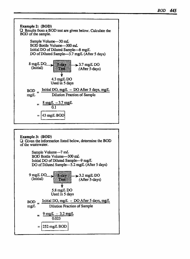
Example 2: (BOD) O Results from a BOD test are given below. Calculate the BOD of the sample.
Sample Volume-30 mL BOD Bottle Volume-300 mL Initial DO of Diluted S ample44 mg/L Do of Diluted Sample-3.7 mg/L (After 5 days)
4.3 mglL DO Used in 5 days
BOD = Initial DO, mg/L - DO After 5 days, mg/L mdL Dilution Fraction of Sample
Example 3: (BOD) C1 Given the information listed below, determine the BOD of the wastewater.
Sample Volume-7 mL BOD Bottle Volume-30 mL Initial DO of Diluted Sample+9 mg/L DO of Diluted Sample-3.2 mg/L (After 5 days)
5.8 mg,L DO Used in 5 days
BOD = Initial DO, mg/L - DO After 5 days, mg/L
mgL Dilution Fraction of S ample

446 Chapter 18 . LABORATORY CALCULATIONS
BOD 7-DAY MOVING AVERAGE
The BOD characteristic of wastewater varies from day to day, even hour-to-hour. However, operational control of the wastewater treatment system is most often accomplished based on trends in data rather than individual data points. The BOD 7-day moving average is a calculation of the BOD trend.
This calculation is called a moving average, since a new 7-day average is calculated each day, adding the new days value and the six previous days values.
BOD 7-DAY MOVING AVERAGE
Day Day Day Day Day Day Day Day Day
4th 7-day Aver.
BOD + BOD + BOD + BOD + BOD + BOD+ BOD 7-day Day 1 Day 2 Day 3 Day 4 Day 5 Day 6 Day 7 Aver. = BOD 7
Example 4: (7-day Moving Average) P Given the following primary effluent BOD test results, calculate the 7day average.
May 1-210 mglL May 5-224 mglL May 2-2 18 mglL May 6-21 6 mglL May 3-202 mglL May 7-220 mglL May 4-207 mglL
BOD + BOD + BOD + BOD+ BOD + BOD+ BOD 7-day Day 1 Day 2 Day 3 Day 4 Day S Day 6 Day 7 Aver. = BOD 7
I BOD I

BOD 447
Example 5: (7-day Moving Average) CI Given the BOD test results shown below, calculate the 7-day average for influent BOD.
BOD + BOD + BOD+ BOD + BOD + BOD + BOD 7-day Day l Day 2 Day 3 Day 4 Day S Day 6 Day 7 Aver. = BOD 7
304 mg/L = I BOD 1
Example 6: (7-day Moving Average) LI Calculate the 7-da average prim effluent BOD for
shown below. J "f; March 12th, 13th, an 14th, given the OD test results
Mar 1-180 Mar G 1 7 2 Mar 11-169 Mar 1 6 1 9 1 Mar 2-174 Mar 7-178 Mar 12-175 Mar 17-187 Mar3---l79 Mar8---l84 Mar13---l87 Mar18-172 Mar 4-185 Mar 9-195 Mar 14---l74 M a r 5 4 8 9 Mar10481 Mar15484
To calculate the 7day average BOD for March 12th, use the test result for March 12th and the 6 days previous (Mar 6-Mar 12):
7-day Aver. 172+ 178+ 184+ 195+ 181+ 169+ 175 BOD = 7
For the next day's average, keep the same string of numbers except drop the "oldest" value (Mar 6) and add the new value (Mar 13):
7-day Aver. l78+ l84 + 195+ 181+ l69+ l7S+ l87 BOD = 7
For the March 14th average, repeat the same process-drop the oldest value and add the new value:
7-day Aver. 184+ 195 + 181 + 169+ 175+ 187+ 174 BOD = 7
SHORTCUT METHOD FOR DETERMINING NEW TOTALS
If you keep track of th total of the 7 days BOD results (the numerator of the average calculation), you may use a shortcut in calculating a new total:
Previous Oldest + New - New 1 - Total Value Value - Total F -
In Example 6, the total in the numerator of the first 7-day average is 1254. To calculate the new total to be used for the next 7-day average:
1254 - 172 + 187 = 1269 Prev. Oldest New New Total Value Value Total

448 Chapter 18 LABORATORY CALCULATIONS
18.2 MOLARITY AND MOLES
A solution is comprised of two parts:
A solvent which is the dissolving medium (such as water), and
A solute which is the substance dissolved (such as dry hypochlorite).
A concentrated solution is one that contains a relatively small amount of solute (e.g., chemical) per unit volume of solution. A dilute solution is one that contains a relatively small amount of solute per unit volume of solution.
The principal methods of expressing the concentrations of solutions are percent strength (see Chapter 14, Section 14.4), molarity (described in this section) and normality (described in the next section). Of these three methods, molarity is perhaps used least often in the field of water and wastewater. However, it has been included here since it may be required occasionally.
Molarity is one method devised to compare solution concen- trations. For example, a solution of one molarity would be one mole of the solute dissolved in one liter. (The concept of "moles" will be discussed later in this section.) A one-molar solution (1M) might also be 2 moles of solute dissolved in 2 liters of solution; or 3 moles solute dissolved in 3 liters solution. It may also be a half mole solute dissolved in a half-liter solution (500 d). Normally, however, we do not fmd such optimum conditions of 1: 1,2:2, etc. Examples 1-3 illustrate how to calculate the molarity of a solution, given the moles solute and solution volume.
MOLARITY IS A WAY TO EXPRESS SOLUTION CONCENTRATION
Liters Solution
Molarity = Moles Solute Liters Solution
Example 1: (Molarity & Moles) P If 2.5 moles of solute are dissolved in 0.5 liters solution, what is the molarity of the solution?
Molarity = Moles Solute Liters Solution
2.5 moles 0.5 liters
= 5 Molarity or 5-Molar Solution
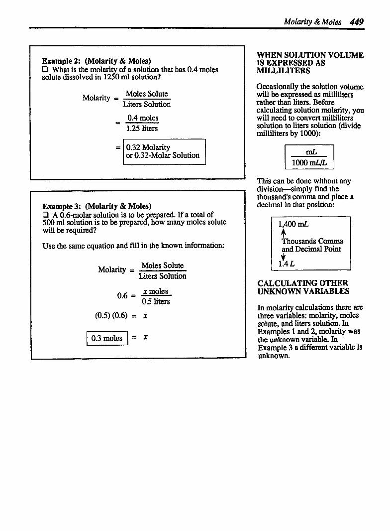
Molarin & Moles 449
Example 2: (Molarity & Moles) P What is the molari of a solution that has 0.4 moles solute dissolved in 12 !?' 0 m1 solution?
Molarity = Moles Solute Liters Solution
- - 0.4 moles 1.25 liters
Example 3: (Molarity & Moles) P A 0.6-molar solution is to be repared. If a total of 500 m1 solution is to be prepare how many moles solute will be required?
(II
=
Use the same equation and fill in the known information:
- - - -
0.32 Molarity or 0.32-Molar Solution
Molarity = Moles Solute Liters Solution
0.6 = X moles 0.5 liters
1 0.3 moles l = X
WHEN SOLUTION VOLUME IS EXPRESSED AS MILLILITERS
Occasionally the solution volume will be expressed as milliliters rather than liters. Before calculating solution molarity, you will need to convert milliliters solution to liters solution (divide milliliters by 1000):
This can be done without any division-simply find the thousand's comma and place a decimal in that position:
1 and Decimal Point I
CALCULATING OTHER UNKNOWN VARIABLES
In molarity calculations there are three variables: molarit y , moles solute, and liters solution. In Examples 1 and 2, molarity was the unknown variable. In Example 3 a different variable is unknown.

450 Chapter 18 . LABORATORY CALCULATIONS
MOLES
Every chemical listed on the Periodic Table of Elements has a corresponding atomic weight listed. The number shown as an atomic weight is an arbitrary number designed to compare the densities of different elements.
The relative densities of the atoms of each elements are more convenient quantities to use than their absolute densities in grams. These relative densities or relative weights are based on an assigned value of exactly 12.0000 for the atomic weight of carbon. From this basis, the atomic weight of each element was assigned by comparing its weight to that of carbon and thus assigning a number higher or lower than 12.
Since atomic weights are used for various calculations in chemistry, it is useful to assign a weight value (that is, grams, pounds, etc.) to the relative weights. A mole is a quantity of a compound equal in weight to its formula weight.
For example, 12 grams of carbon would be one gram-mole of carbon. And 12 pounds of carbon, is a pound-mole of carbon. In water and wastewater calcula- tions, we are primarily concerned with gram-moles. The term "mole" will be understood to mean "gram-mole ". To calculate the number of moles used in preparing a solution, use the following equation:
Molarit y Grams of Chemical = Formula Wt. of Chemical
A MOLE IS A QUANTITY OF A COMPOUND EQUAL IN WEIGHT IY) ITS FORMULA WEIGHT
For example, the formula weight for water (H20) can be determined using the Periodic Table of Elements:
Hydrogen (1.008) X 2 = 2.01 6 Oxygen = 16.000
Formula weight + 18.016 ofHzO
Since the formula weight of water is 18.0 16, a mole is 18.016 units of weight. A gram-mole is 18.016 grams of water. A pound-mole is 18.016 pounds of water.
Example 4: (Molarity & Moles) P The atomic weight of calcium is 40. If 65 grams of calcium are used in making up a one-liter solution, how many moles are used?
Moles = Grams of Chemical Formula wt.
- 65 grams 40 grams/mole

Molar@ & Moles 451
Example 5: (Molarity & Moles) P If magnesium has a listed atomic weight of 24, how many moles is represented by 62 grams of magnesium?
Moles = Grams of Chemical Formula wt.
- - 62 grams 24 grams/mole
= 1 2.6 moles I
Example 6: (Molarity & Moles) O The atomic weights listed for each element of sulfuric acid (&SO4) are given below. How many gnuns make up a mole of sulfuric acid?
To determine the formula weight of sulfuric acid, the total weight of each element must be calculated:
Atomic Number of Total Weight Element Weight Atoms Represented
H: 1.008 X 2 = 2.016
DETERMINING FORMULA WEXGHT OF A COMPOUND
To calculate the f o d a weight of a compound, first determine the total atomic weight represented by each element. Then total a l l these weights to obtain the formula weight. Example 6 illustrates this type of calculation.

452 Chapter 18 LABORATORY CALCULATIONS
18.3 NORMALITY AND EQUIVALENTS
The molarity of a solution refers to its concentration (the solute dissolved in the solution). The normality of the solution refers more specifically to the reacting power of the solution. One of the first concepts to be learned in a basic chemistry course is that the sharing or transfer of electrons is responsible for chemical activity or the reacting characteristics of an element or compound
The concept of equivalents parallels this concept by relating the number of electrons available to be transferred or shared (valence) and the atomic weight associated with each of these valence electn>ns.*
Since the concept of equivalents is based upon the "reacting power" of an element or compound, it follows that a specific number of equivalents of one substance will react with the same number of equivalents of another substance. For example, two equivalents of a substance will react with two equivalents of another substance. If, however, one equivalent of Substance A is mixed with two equivalents of Substance B, only one equivalent of each substance will react, leaving an excess of one equivalent of Substance B.
Practically speaking, if the concept of equivalents is ignored when making up solutions, most likely chemicals will be wasted as excess amounts.
NORMALITY IS A MEASURE OF THE "REACTING POWER" OF A SOLUTION
With
Normality = No. of Equivalents of Solute Liters of Solution
This equation may be rearranged as:
(Normality) (Liters) = Equivalents of Sol'n Sol'n in Solution
Example 1: (Normality and Equivalents) P If 2.5 uivalents of a chemical are dissolved in 1 .5 liters solution, "% W at is the normality of the solution?
Normality = No. of Equivalents of Solute Liters of Solution
- - 2.5 Equivalents 1.5 liters
* The valence number may be either positive or negative, depending upon whether electrons were added to or taken from the particular element or compound.

Normulity & Equivalents 453
Example 2: (Normality and Equivalents) O A 600-m1 solution contains 1.8 equivalents of a chemical. What is the nomality of the solution?
First convert 600 mL to liters:
Then calculate the normality of the solution:
Normality z No. of Equivalents of Solute
Liters of Solution
- - 1.8 Equivalents 0.6 Liters
Example 3: (Normality and Equivalents) O How man milliliters of 0.5 N NaOH will react with 500 m. of o.& N HCl?
Set the normality and volume of the first solution equal to the normality and volume of the second solution:
WHEN MILLILITERS VOLUME IS GIVEN
Many times the volume of solution is given as milliliters. To calculate normality, the volume must be expressed in liters. Therefore, convert the di l i ters volume to liters:
(mL) (l liters) = liters l 1WOmL.
NORMALITY AND TITRATIONS
The second equation, given on the previous page, indicates that the normality of a solution times the volume of the solution is equal to the number of equivalents in the solution:
l (Normality) (Volume) = No. of of S o h L Equiv. 1
Because chemicals react on the basis of equivalents, this relationship is of great importance in understanding titrations (such as used in the COD test) or acid/base neutralizations. In general, where N = normality of the solution and V = volume of the solution:
When using this equation, the so- lution volume may be expressed as liters or milliliters. However, whichever term (m1 or L) is used on one side of the equation, must also be used on the other side of the equation.

454 Chapter I8 LABORATORY CALCULATIONS
EQUIVALENT WEIGHT Example 4: (Normality and Equivalents) O If oxygen has an atomic weight of 16 and has 2 valence electrons, what is the equivalent weight of oxygen?
Equivalents relate the number of valence electrons (electrons that may be shared or transferred) with a corresponding atomic weight. Although knowing how to determine the number of valence electrons is not required in water and wastewater calculations, a general understanding of how equivalents are calculated will help you better understand the concept of normality. Examples 4-7 illustrate the calculation of equivalents.
v 1 Valence 1 Valence Electron Electron
16 Equivalent = - Weight 2
Equivalent - - Atomic Weight Weight Net Valence
Example 5: (Normality and Equivalents) P If aluminum has an atomic weight of 27 and has a valence of 3, what is the equivalent weight of aluminurn?
This equation may be stated in more general terms to include compounds:
Equivalent - Fornulaweight Weight - Net Valence
1 Valence 1 Valence 1 Valence Electron Electron Electron
Equivalent = 27 Weight 3

Normality and Equivalents 455
Example 6: (Normality and Equivalents) O The molecular weight of NazCQ is 106. The net valence is 2. If 90 grams of Na2C03 are dissolved in a solution, how many equivalents are dissolved in the solution?
The equivalent weight of Na2 C% is 106 + 2 = 53. Calculate the number of equivalents as follows:
Number of = of NIOH Equivalents Equivalent wt.
= 1 1.7 Equivalents I
Example 7: (Normality and Equivalents) C3 Given the atomic weights and net valence of NaOH, what is the normality of an 800-mL solution in which 45 grams of NaOH are dissolved?
.............. S odium (Na) .23 ............... Oxygen (0). 16
Hydrogen (H) ............... 1 Net Valence = 1
The equivalent weight of NaOH is 40 + 1 = 40. First calculate the number of equivalents dissolved in the solution:
Number of = MOH Equivalents Equivalent wt.
The normality of the solution can now be determined:
Normality = NO. of Equivalents of NaOH Liters of Solution
- l, f 25 Euuivalents 0.8 Liters
CALCULATING NUMBER OF EQUIVALENTS
To determine the number of equivalents used in a solution, you will need to know the grams of chemical used and the equivalent weight:
Number of , chemicals gramS Equivalents Equivalent wt.
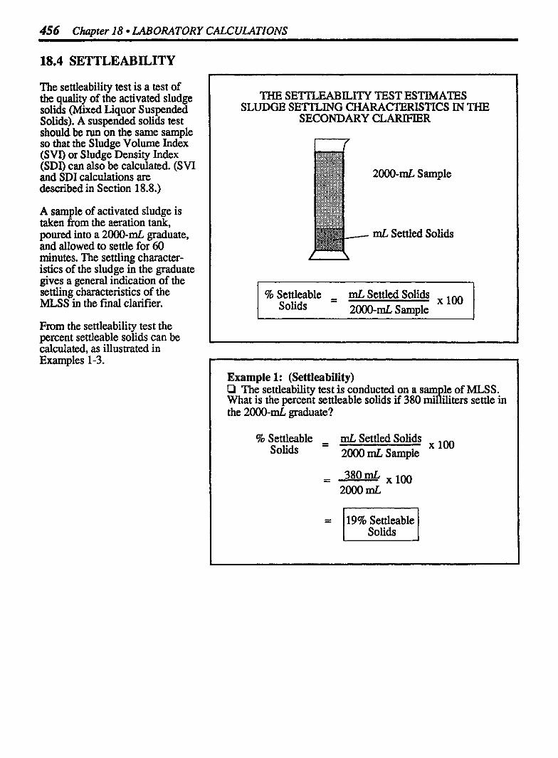
456 Chapter 18 LABORATORY CALCULATIONS
18.4 SETTLEABILITY
The settleability test is a test of the quality of the activated sludge solids (Mixed Liquor Suspended Solids). A suspended solids test should be run on the same sample so that the Sludge Volume Index (SVI) or Sludge Density Index (SDI) can also be calculated. (SW and SDI calculations are described in Section 1 8.8 .)
A sample of activated sludge is taken from the aeration tank, poured into a 2000-mL graduate, and allowed to settle for 60 minutes. The settling character- istics of the sludge in the graduate gives a general indication of the settling characteristics of the MLSS in the final clarifier.
From the settleability test the percent settleable solids can be calculated, as illustrated in Examples 1 -3.
THE SETTLEABILITY TEST ESTIMATES SLUDGE SE'ITLING CHARACTERISTICS IN THE
SECONDARY CLARIFIER
% Settleable - - mL Settled Solids Solids 2000-mL Sample
Example 1: (Settleability) Ll The settleability test is conducted on a sam le of MLSS. What is the percent settleable solids if 380 & ters settle in
the 2000-ml, graduate?
% Settleable - mL Settled Solids Solids 2000 mL. Sample
= 19%Settleable I Solids
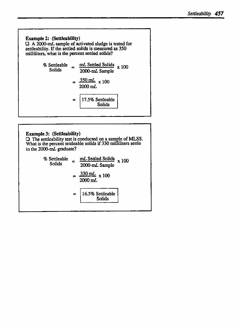
Settleability 457
Example 2: (Settleability) LI A 2000-mL sample of activated sludge is tested for settleability If the settled solids is measud as 350 milliliters, what is the percent settled solids?
% Settleable - mL Settled Solids 100 Solids 2000-11121 S ample
= I 17.5% Settleable / Solids
Example 3: (Settleability) O The settleability test is conducted on a sam le of MLSS.
in the 2000-mL graduate? Jo What is the percent settleable solids if 330 fiters settle
% Settleable - - mL Settled Solids Solids 2000-mL, Sample
= 16.5% Settleable 1 Solids 1

458 Chapter 18 LABORATORY CALCULATIONS
18.5 SETTLEABLE SOLIDS (IMHOFF CONE)
The settleable solids test, like the settleability test, measures the volume of solids that settle out from a wastewater sample during the 601minute test. This test differs from the settleability test in at least two respects:
The settleable solids test is conducted in a one-liter Imhoff Cone. (The settleability test or settled sludge volume test, is conducted in a one-liter or two-liter graduated cylinder.)
The settleable solids test is conducted on samples from sedimentation tank or clarifier influent and effluent. (The settleability test or settled sludge volume test is conducted on samples from the activated sludge aeration basin.)
This test indicates the volume of solids removed by sedimentation in sedimentation tanks, clarifiers, or ponds.
By running a settleable solids test on the wastewater influent and effluent, the settleable solids test can be used to estimate the percent removal of settleable solids.
THE SETTLEABLE SOLIDS TEST IS CONDUCTED IN A ONE-LITER IMHOFF CONE
THIS TEST IS CONDUCTED ON SEDIMENTATION TANK INFLUENT AND EFFLUENT TO DETERMINE
% REMOVAL OF SET SOL.
Influent Effluent Settleable + + Settleable
Solids Solids ( m u ) (mUL)
Removed Settleable Solids, mLIL
% Removal - Set. Sol Removed, &L 100 of Set. Sol. in Influent, mLJL
Example 1: (Settleable Solids) P Calculate the percent removal of settleable solids if the settleable solids of the sedimentation tank influent is 17 mUL and the settleable solids of the effluent is 0.3 N L .
16.7 mL/L Set. Sol. Removed
= 1 989 Set. Sol. I Removed
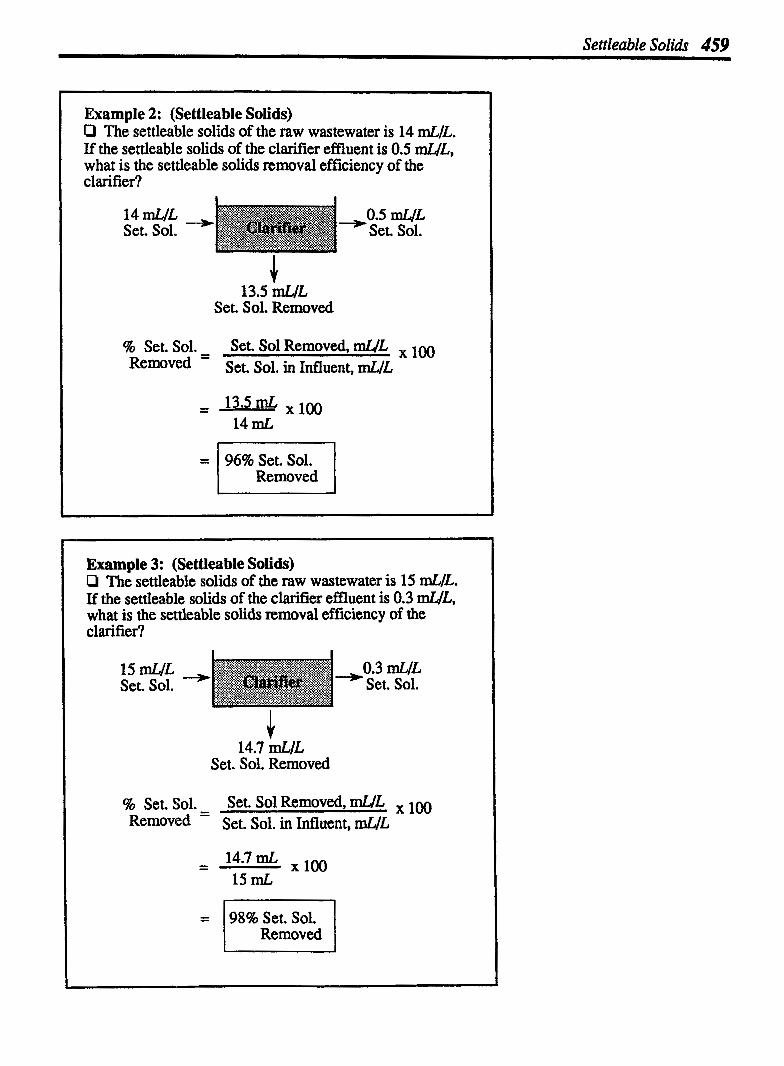
Settleable Solids 459
Example 2: (Settleable Solids) O The settleable solids of the raw wastewater is 14 mUL. If the settleable solids of the clarifier effluent is 0.5 mUL, what is the settleable solids removal efficiency of the clarifier?
13.5 mCJL Set. Sol. Removed
% Set. Sol. - Set. Sol Removed, mL/L , Removed - Set. Sol. in Influent, mLJL
Example 3: (Settleable Solids) 0 The settleable solids of the raw wastewater is 15 mLJL. If the settleable solids of the clarifier effluent is 0.3 mUL, what is the settleable solids removal efficiency of the clarifier?
=
14.7 &L Set. Sol. Removed
96% Set. Sol. Removed
% Set.So1. - Set.SolRemovedmL/L Fkmoved - Set. Sol. in Influent, mLJL
= 98% Set. Sol. l Removed

460 Chapter 18 LABORATORY CALCULATIONS
18.6 SLUDGE TOTAL SOLIDS AND VOLATILE SOLIDS
Wastewater is comprised of both water and solids. The total solids may be further classified as either volatile solids, representing the organics, or fixed solids, repre- senting the inorganics in the wastewater. This relationship must be clearly understood prior to any mathematical calculations regarding total solids content, fixed solids content, volatile solids content, or moisture content of any particular wastewater. These calculations may be expressed in terms of percent solids(b y weight) or mg/L concentrations. Normally, total solids and volatile solids are expressed as percents; whereas suspended solids are generally expressed as mglL.*
In calculating either percents or mglL concentrations, certain concepts must be understood:
Total Solids The solids remaining after drying wet sludge overnight at 103' - 105' C.
Fixed Solids The solids remaining after burning for 1 hour at 600' C.
Volatile Solids The solids which are destroyed or lost through the l-hour burning period.
This relationship may be expressed graphically as shown to the right. Percent total solids and volatile solids are calculated as follows:
% Volatile = Vol. Solids Wt. Solids Tot. Solids wt.
TOTAL AND VOLATILE SOLIDS
Fixed Solids (Inorganics)
Volatile Solids (Organic S)
Water
Total Solids
UNDERSTANDING THE TERMS IS ESSENTIAL
Volatile
ds
Solids (Remaining -
Ash)
When the word "sludge" is used, it may be understood to mean a semi-liquid mass composed of solids and water. The term "solids" is used to mean dry solids after the evaporation of water.
* For a review of mg/L to % conversions, refer to Chapter 8.

Sludge Total and Volatile Solids 461
Example 1: (Sludge Total and Volatile Solids) O Given the information below, (a) determine the
solids in the sludge sample: Ft total solids in the sample, and (b) the percent of vo atlle
Sludge After (Total After Burning
Sample) Drying (Ash)
Wt. of Sample & Dish 71.82 g 24.57 22.95 Wt. of Dish (tare wt.) 22.08 g 22.08 22.08
a) To calculate % total solids, the grams total solids (solids after drying) and grams sludge sample must be determined:
Total Solids Sludpe Sam~le 24.57 g Total Solids & Dish 71.82 g Sludge & Dish
- 22.08 g Wt of Dish - 22.08 g Dish 2.49 g Total Solids 49.74 g Sludge
% Total = Wt. of Total Solids 100 Wt.ofSludgeSample
- 2.49 grams - 49.74 grams
= 15% Total Solids I
b) To calculate the % volatile solids, the gram ,S total solids &d grams volatile solids must be determined. Since total solids has already been calculated in Part a, only volatile solids must be calculated:
Volatile Solids
24.57 g Sample and Dish Before Burning 22.95 g Sample and Dish After Burning
1.62 g Solids Lost in Burning
% Vol. Wt. of Volatile Solids Solids Wt. of Total Sample
= ( 65% Volatile Solids I

462 Chapter 18 LABORATORY CALCULATIONS
Example 2: (Sludge Total and Volatile Solids) P Given the information below, calculate (a) the percent total solids and (b) percent volatile solids of the sludge sample.
Sludge After (Total After Burning
Sample) Drying (Ash) Wt. of Sample & Dish 69.82 g 22.04 20.46 Wt. of Dish (tare wt.) 19.79 g 19.79 19.79
a) To calculate % total solids, the grams total solids (solids after drying) and grams sludge sample must be determined:
Total Soli& Sludge Sample 22.04 g Total Solids & Dish 69.82 g Sludge & Dish
- 19.79 g Wt of Dish - 19.79 g Dish 2.25 g Total Solids 50.03 g Sludge
% Total = Wt.ofTotalSolids Solids Wt. of Sludge Sample
- 2.25 grams 50.03 grams
b) To calculate the % volatile solids, the grams total solids and grams volatile solids must be determined. Since total solids has already been calculated in Part a, only volatile solids must be calculated:
Volatile Solids
22.04 g Sample and Dish B e f o ~ Burning - 20.46 g Sample and Dish Afhr Burning
1.58 g Solids Lost in Buming
qb ~ o t a l = Wt. of Volatile Solids Solids Wt. of Total Sample

Sludge Total and Volatile Solids 463
Example 3: (Sludge Total and Volatile Solids) P In Exam le 2, the 100-m1 sludge sample was found to contain 1.5 grams volatile solids. What is this expressed as mdL?
rP
Example 4: (Sludge Total and Volatile Solids) O A 100 m1 sludge sample has been dried and burned. Given the information below, a) determine the percent volatile solids content of the sample, and b) determine the mglL concentration of the volatile solids.
After After Drying Burning (Ash)
Wt. of S ample & Crucible 22.0 153 g 22.0067 g Wt. of Cruciblc (tare wt.) 22.0021 g 22.002 1 g
a) To calculate % volatile solids, you will first need to know grams volatile solids and grams total solids:
Total Solids 22.01 53 g Sample & Crucible After Drying
- 22.0021 g Crucible Wt 0.0132 g Total Solids
Volatile Solids 22.0153 g Sample & Crucible Before Burning
- 22.0067 g Sample & Crucible ,After Burning 0.0086 g Volatile Solids
% volatile , Wt. of volatile Solids Solids Wt. of Total Solids
= 1 65% Volatile Solids I b) Express the volatile solids content as mglL:
CALCULATING mglL TOTAL AND VOLATILE SOLIDS
The results of the total and volatile solids may be expressed as mglL. To do this, the grams total or volatile solids must be known as well as the volume of sludge sample (milliters). Since sludge samples are generally 100 milliliters, mg/L is calculated as shown below.
SteD 1 Step 2
In Step 1, grams solids (total or volatile) are converted to milli- grams solids. Note that only the numerator is multiplied by 1000 since grams are simply being reexpnssed as an equivalent number of milligrams. The numerator is now in the desired terms.
The denominator is desired in liters. To obtain liters, the deno- minator (100 ml) must be multi- plied by 10. Since this is not a conversion of terms, if the deno- minator is multiplied by 10, the numerator must also be multiplied by 10. (Multiplying by 10/10 does not change the overall value of the fraction because 10/10 = 1 .)
Examples 3 and 4 illustrate the calculation of mglL total or volatile solids using sludge sample data.

464 Chapter 18 LABORATORY CALCULATIONS
18.7 SUSPENDED SOLIDS AND VOLATILE SUSPENDED SOLIDS (OF WASTEWATER)
The total and volatile solids of sludge are generally expressed as percents, by weight. The sludge samples are 100 ml, and are unfiltered.
The suspended solids test is designed to measure the solids load or the strength of the wastewater by measuring the suspended particles in the water. Because the solids are filtered from the sample, often the sample is limited to 50 mL, to prevent clogging of the filter.
Except for the required drying time, the suspended solids and volatile suspended solids tests of wastewater are similar to those of the total and volatile solids perfomed for sludges (described in the previous section).
Suspended solids are normally reported as milligrams per liter (mglL) whereas volatile suspended solids are normally given as a percent (%). The equations for these calculations are described on the facing page. Note the similarity between these equations and those used in the previous section for sludge total solids and volatile solids.
SUSPENDED SOLIDS AND VOLATILE SUSPENDED SOLIDS
Volatile Suspended
s T &
- Ash)
Example 1: (SS & VSS) P Given the following information regarding a primary effluent sample, (a) calculate the mg/L suspended solids, and (b) the percent volatile suspended solids of the sample.
After Drying After Burning (Before Burning) (Ash)
Wt. of Sample & Dish 24.6862 g 24.6830 g Wt. of Dish (tare wt.) 24.6820 g 24.6820 g Sample Volume = 50 mZ.
a) To calculate the milligrams suspended solids per liter of sample (mglL), you must first detedne grams suspended solids:
24.6862 g Dish and Suspended Solids - 24.6820 g Dish
0.0042 g Suspended Solids
Now mglL suspended solids can be calculated:
b) To calculate percent volatile suspended solids, you must know the weight of both total suspended solids (calculated in part "a" above) and volatile suspended solids.
24.6862 g Dish & SS Before Burning - 24.6830 g Dish & SS After Burning
0.0032 g Solids Lost in Burning
Wt.ofVol.Solids xlOO %VSS =
Wt. of Susp. Solids
- - 0.0032 g VSS 0.0042 g SS
* Multiplication factor used to make the denominator equal to 1 liter (1000 d). This number will vam with sample volume.
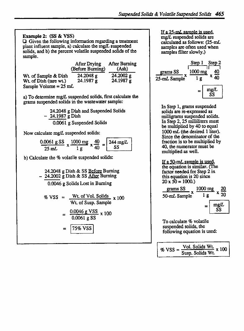
Suspended Solids & Volatile Suspended Solids 465
Example 2: (SS & VSS) O Given the following information regarding a treatment plant influent sample, a) calculate the mg/L suspended solids, and b) the percent volatile suspended solids of the sample.
After Drying After Burning (Before Burning) (Ash)
Wt. of Sample & Dish 24.2048 g 24.2002 g WtofDish(tarewt.) 24.1987g 24.1987 g Sample Volume = 25 mL,
a) To determine mglL suspended solids, fvst calculate the grams suspended solids in the wastewater sample:
24.2048 g Dish and Suspended Solids - 24.1987 g Dish
0.0061 g Suspended Solids
Now calculate mg/L suspended solids:
b) Calculate the % volatile suspended solids:
24.2048 g Dish & SS Before Buming - 24.2002 g Dish & SS ,After Burning
0.0046 g Solids Lost in Burning
% v s s = Wt.ofVol.Solids Wt. of Susp. Sample
- - 0.0046 g VSS ,100 0.0061 g SS
If a 25-mL, sample is used, mglL suspended solids are calculated as follows: (25-mL samples are often used when samples filter slowly.)
In Step 1, grams suspended solids are reexpressed as milligrams suspended solids. In Step 2,25 milliliters must be multiplied by 40 to equal loo0 mL, (the desired 1 liter). Since the denominator of the fraction is to be multiplied by 40, the numerator must be multiplied as well.
f a 50- le i Le equZo:YLdY&e factor needed for Step 2 in this equation is 20 since 20 X 50 = 1000.)
X 50-mL, Sample l g
To calculate % volatile suspended solids, the following equation is used:
Vol. Solids Wt. 100 % VSS =
Susp. Solids Wt.
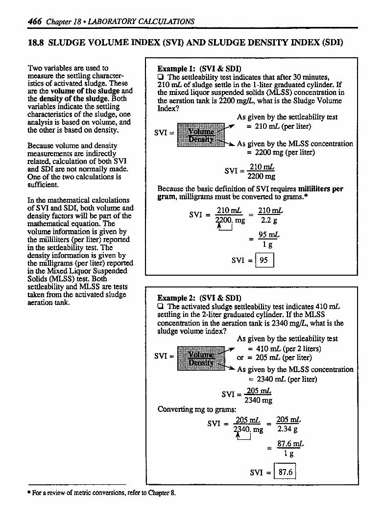
466 Chapter 18 LABORATORY CALCULATIONS
18.8 SLUDGE VOLUME INDEX (SW) AND SLUDGE DENSITY INDEX (SDI)
Two variables are used to measure the settling character- istics of activated sludge. These are the volume of the sludge and the density of the sludge. Both variables indicate the settling characteristics of the sludge, one analysis is based on volume, and the other is based on density.
Because volume and density measurements are indirectly related, calculation of both SVI and SDI are not normally made. One of the two calculations is sufficient.
In the mathematical calculations of SVI and SDI, both volume and density factors will be part of the mathematical equation. The volume information is given by the milliliters (per liter) reported in the settleability test. The density information is given by the milligrams (per liter) reported in the Mixed Liquor Suspended Solids (MLSS) test. Both settleability and MLSS are tests taken from the activated sludge aeration tank.
Example l: (SVI & SDI) Q The settleability test indicates that after 30 minutes, 2 10 mL of sludge settle in the l -1iter graduated cylinder. If the mixed liquor suspended solids (MLSS) concentration in the aeration tank is 2200 mglL, what is the Sludge Volume Index?
As given by the settleability test
= 2200 mg (per liter)
Because the basic definition of SVI requires milliliters per gram, milligrams must be converted to grams.*
SVI =
Example 2: (SVI & SDI) P The activated sludge settleability test indicates 410 mL, settling in the 2-liter graduated cylinder. If the MLSS concentration in the aeration tank is 2340 mglL, what is the sludge volume index?
As given by the settleability test
= 2340 rnL (per liter)
Converting mg to grams:
* For a review of metric conversions, refer to Chapter 8.

Sludge Volwne Index & Sludge Density Index 467
Example 3: (SVI & SDI) Cl The settleability test indicates that after 30 minutes, 390 mL of sludge settle in the 2-liter graduated cylinder. If the mixed liquor suspended solids (MLSS) concentration in the aeration tank is 2170 mglL, what is the sludge volume index?
As given by the settleability test
= 2 170 mg (per liter)
SVI = 195 mL
2170 mg
Because the basic definition of SVI requires milliliters per gram, milligrams must be converted to grams.**
SVI = 195 mL 195 = -
$l7Oi mg 2.17 g
SVI = 1 90 ]
Example 4: (SVI & SDI) P The activated sludge settleability test indicates 440 mL settling in the 2-liter graduated cylinder* If the MLSS concentration in the aeration tank is 2610 mglL, what is the sludge volume index?
As given by the settleability test = 440 mL (per 2 liters)
As given by the MLSS concentration = 26 10 mL (per liter)
SVI = 220 mL 2610 mg
Converting mg to grams:
SVI = 220 mL 220 mL = - 2610mg 2.61g A i
SVI = 1 84 1
SLUDGE VOLUME INDEX ( S W
In calculations of SVI, volumes are being compared and volume is in the numerator of the SVI equation:
SW = Volume, rnL Density, g
SVI is defined as the milli- liters volume occupied by 1 gram of activated sludge after a 30-minute settling period**
* Normally the SW of a good quality activated sludge will range from 50-100. As the Index increases to 200 or more, the sludge is considered to be bulked sludge.

468 Cha~ter 18 LABORATORY CALCULATIONS
SLUDGE DENSITY INDEX
The calculation of sludge density index (SDI) is different from that of sludge volume index (SW) in two respects:
The numerators and denomin- ators are "flipped". For SDI, the density data is in the numerator, whereas for SVI the volume data is in the numerator, and
The fraction must be multiplied by 100, since SDI is essentially a percent calculation.* This is reflected by the definition of SDI.
SDI is defined as the concentra- tion, in percent solids, which the activated sludge will assume after 30 minutes settling. Examples 5-8 illustrate the SDI calculation.
Density, g SDI = X 100
Volume, mL
To remember whether density or volume goes in the numerator of SVI and SDI, simply remember that volume goes in the numerator of sludge volume index (SVI), and density goes in the numerator for sludge density index (SDI).
Example 5: (SVI & SDI) Cl The MLSS concentration in the aeration tank is 2400 mgb. I€ the activated sludge settleability test indicates 215 mL, settled in the one-liter graduated cylinder, what is the sludge density index?
SDI = 2400mg .loo 215 mL
Convert the mg to grams:
U SDI = = - 2*4g X100
215mL 215mL
Example 5: (SVI & SDI) C] The MLSS concentration in the aeration tank is 1980 mglL. If the activated sludge settleability test indicates 175 ml. settled in the one-liter graduated cylinder, what is the sludge density index?
1980 m SDI = g X 100
175 mL Convert the mg to grams:
4-l 1.98 g SDI = = - x100 175 mL 175 mL
* For a review of percents, refer to Chapter 5 in Basic Math Concepts.

Sludge Volume Index & Sludge Density Index 469
Example 7: (SVI & SDI) LI The sludge volume index for a sludge is known to be 85. What is the sludge density index for that sludge?
loo SDI = - SW
Example 8: (SVI & SDI) Q The SVI for a sludge is 72. If the settleability test indicates that 195 mL of sludge settles in the l-liter graduated cylinder, what must be the MLSS concentration, in mglL?
Use the same equation as usual, filling in the known information. First solve for grams, then convert to milligrams (m& MLSS):
SW = Volume, mL Density, g
or = l 2 7 w m g l ~ I MLSS
If the SVI value is known, the SDI can be calculated as follows:
loo SDI = -
Example 7 illustrates this type of calculation.
CALCULATING OTHER UNKNOWN VALUES
SVI and SDI calculations involve three variables: SVI (or SDI), rnilliliters, and grams. In Examples 1-7, either SVI or SDI were the unknown variables. In fact, any one of the three variables can be the unknown factor, Example 8 illustrates calculations of this type.

470 Chapter 18 LABORATORY CALCULATIONS
18.9 TEMPERATURE
Since the temperature of the wastewater affects its general characteristics, this test is one of the most frequently performed tests. The formulas normally used to convert Fahrenheit (OF) to Celsius 'C, are as follows:
Fahrenheit to Celsius: "C = 5/9 (OF-32O)
Celsius to Fahrenheit: 'F = 915 ('C) + 32'
Because these formulas have parentheses around different terms, and one requires the addition of 32' while the other requires the subtraction of 32O, they are very difficult conversions to remember unless used constantly . Another method of converting these two terms is more easily remembered and can be used regardless of whether the conversion is from Fahrenheit to Celsius or vice versa. This method consists of three steps, as illustrated at the top of this page.
Step 2 involves the only variable in these conversions. The decision of whether to multiply by 5/9 or 915 is dependent whether a larger or smaller number is desired.
The Celsius temperature scale is a lower range scale than that of Fahrenheit. For example, the boiling point of water (at sea level) expressed in Fahrenheit is 2 12O; W hercas the boiling point expressed in Celsius is 100". Therefore, when converting O0 Celsius to Fahrenheit, the answer should be greater than 0'. W hen converting 80' Fahrenheit to Celsius, the answer should be less than 80'.
THE THREE-STEP METHOD OF TEMPERATURE CONVERSION
Step l: Add 40° Step 2: Multiply by 5/9 or 9/5
(Depending on direction of conversion.)
Step 3: Subtract 40'
THE EFFECT OF MULTIPLYING BY 5/9 OR 915
When multiplying by 519 (approximately 1/2), the answer will be less than the original number. For example:
Compare
When multiplying by 915 (approximately 2), the answer will be greater than the original number. For example:
Compare

Temperature 471
Example 1: (Temperature) P The influent to a treatment plant has a tern rature of 75' F. What is this temperature expressed in gees Celsius?
E Step 1: (Add 40')
Step 2: (Multiply by 5/9 or 915)
In this example the conversion is from Fahrenheit to Celsius. Since the answer should be a smaller number, multiply by 519:
Step 3: (Subtract 40')
Example 2: (Temperature) O The effluent of a treatment plant is 23' C. What is this expressed in degrees Fahrenheit?
Step 1: (Add 40') 23'
+ 40° - 63'
Step 2: (Multiply by 5/9 or 915)
In this example the conversion is from Celsius to Fahrenheit. Since the answer should be a larger number, multiply by 915:
= 113' Step 3: (Subtract 40')


p- P
Area and Volume Equations-Metric System
1. Areas
The equations for the four basic shapes most often used in area calculations are as follows:
Rectangle , where:
Triangle A -
Trapezoid
Circle
A = area, m2 I = length, m
W = width, m
where:
A = area, m 2
b = base, m h = height, m
where:
A = area, m2 b l = smaller base, m b 2 = larger base, m h = height, m
2. Volumes
The equations for the five basic shapes most often used in volume calculations are given below. The equation for oxidation ditch volume is also given.
Rectangular Prim I
V = Iwh
h V = volume. m3 l = length, & I V w - w = width, m
fl- h = height, m
Triangular Prism
b = base, m h = height, m l = length, m
Trapezoidal Prism
2 where:
V = volume, rn3 b 1 = smaller base, m b 2= larger base, m h = height, m l = length, m

VOLUME EQLIATIONS--METRlC SYSTEM 475
Cylinder
V = (0.785) (D ) (h.)
where:
V = volume, m 3
D = diameter, m h = height, m
Cone
where:
V = volume, m 3
D = diameter, m h = height, m
Oxidation Ditch
Top View Dashed line represents total ditch length (L) . This is equal to 2 half circmferences + 2 lengths
Cross-Section
volume, (Trapezoidal) (Total LRngth) cu ft Area
W here: 3 V = volume, m
b 1 = smaller base, m b 2= larger base, m h = height,m l = length, m

Preliminary Treatment - Metric System
Screenings Removed
Screenings screenings, m3 Removed = (d Iday day
Screenings - screenings, L Removed - (Um3
flow, m3
2. Screenings Pit Capacity
Screening pit - screening pit vol., m3 capacity, &Y S- screening removed, m 3/d
Grit Channel Velocity
Two equations may be used to estimate the velocity of flow through the grit channel. The first equation is the Q=AV equation.
Q = (width) (depth) (velocity) m3/s m m m/s
The second equation is required when using a float or dye to time the velocity of flow.
Velocity = distance traveled, m test time, S
4- Particle Settling Rate
Settling Rate, m/s = depth, m settling time, S
5. Water Depth, Velocity and Channel Length
The equation often used to determine required channel length to permit particle settling is:
(channel depth) (flow velocity) Length, - m
m m/sec
ill
Settling Rate, m/s
To make this equation easier to remember, it can be rearranged as shown below:
channel length, m - - flow velocity, m/s channel depth, m settling rate, m/s
6. Grit Removal
Grit Removal = ~ / m 3 flow, m3
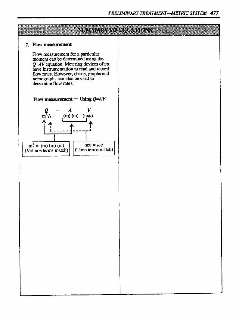
7. Flow measurement
Flow measurement for a particular moment can be determined using the Q=AV equation. Metering devices often have instrumentation to read and record flow rates. However, charts, graphs and nomographs can also be used to determine flow rates.
Flow measurement - Using Q=AV
sec = sec I (Time terns match)

Sedimentation- Metric System
1. Detention Time
Detention - tank volume, m Time, hrs -
flow, m3/h
2. Weir Overflow Rate
Weir Ovelnow Rate = floy, m3/d welr, m
3. Surface Overflow Rate
Surface Overflow - - flow, m3/d Rate area, m2
(Swface overjlow rate does not include recirculated jZo ws.)
4. Solids Loading Rate on Clarifier
Simplified Equation:
"lids solids applied, kg/d Loading = Rate surface area, m2
Expanded Equation:
(MLSS ) (Plant + RAS) mg/L flow, m3/d
Solids Loading = loo0
Rate (0.785) (D2 )
5. BOD and Suspended Solids Removed
First calculate BOD or SS removed. m&:
Influent - Effluent = Removed SSmg/L SSmg/L SSmgL
Then calculate kdd BOD or SS removed;
BOD or SS Removed
6. Dry Sludge Solids Produced, lbslday
7. Percent Solids and Clarifier Sludge Pumping
This equation is sometimes rearranged for use in kg/d sludge calculations:
Sludge, kg/d = solids, kg/d % solids

SEDIMENTATIONIIAETRIC SYSTEM 479
8. Unit Process Efficiency
%SS = SS removed, mg/L Removed SS total, m@
% BOD = BOD removed. m J L 1 ( Removed B o D total, m e

Trickling Filters - Metric System
1. Hydraulic Loading Rate
(Hydraulic loading rate calculations include recirculated flo ws .)
Organic Loading Rate
Simplified Equation:
Organic Loading - kdd BOD Rate -
m3
Expanded Equation:
1 (mg/L BOD) (m3/d flow)
3. BOD and SS Removal, lbslday
First calculate mg/L BOD or SS removed:
BODorSS BODorSS BODorSS in Influent - in Effluent = Removed
(m@) (m@) (ma)
Then calculate kg/d BOD or SS removed:
(m& BOD or SS) (m3/d flow) Removed kg/d
= BOD or 1 loo0 SS Rem.
4. Unit Process or Overall Efficiency
Unit Process Efficiencv;
% S S = m& SS Removed Removed m@ SS Total
% BOD = W!L BOD Removed 100 Removed mg/L BOD Total
Overall Efficiency:
First calculate m& BOD or SS removed:
BODorSS BODorSS BODorSS in Influent - in Effluent = Removed (m&) (m&) (m&)
Then calculate the overall efficiency:
% Overall - m@ BOD or SS Removed Efficiency - mg/L BOD or SS in Influent
5. Recirculation Ratio
Recirculation Recirculated Flow, m3 /d Ratio - Plant Influent Flow, m3/d
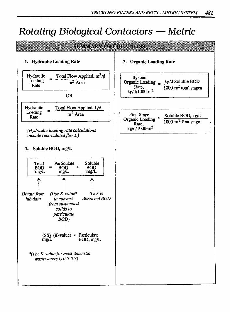
TRICKLING FILTERS AND RBCOMETRIC SYSTEM 481
Rotating Biological Contactors - Metric
I. Hydraulic Loading Rate
Hydraulic - Total Flow Applied, m3/d Loading -
Rate m2 Area
Hydraulic - Total Flow Applied, L/d Loading -
Rate m2 Area
(Hydraulic loading rate calculations include recirculated flows.)
2. Soluble BOD, m@
Total Particulate Soluble BOD = BOD + BOD
m g n mgf'L
Obtain from (Use K-value* This is i lab data to convert dissolved BOD I from suspended
solids to particulate
BUD)
I (SS (K-value) = Particulate m k BOD, mgn
*(The K-value for most domestic wastewaters is 0.5-0.7)
3. Organic Loading Rate
System organic Loading = kdd Soluble BOD I - -
Rate, 1000-m2 total stages I kg/~~im-1112
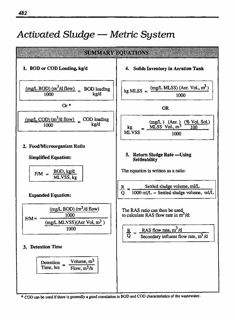
Activated Sludge - Metric System
1. BOD or COD Loading, kg/d
(m* BOD) (m3/d flow) - - BOD loading loo0 kg/d
Or*
( m a COD) (m3/d flow) - COD loading loo0 - kgld
2. Food/Microorganism Ratio
Simplified Equation:
BOD, kg/d MLVSS, kg
Expanded Equation:
I (m@ BOD) (m3/d flow) I loo0
(mg/L MLVSS)(Aer Vol, m3 )
3. Detention Time
Detention - Volume, m3 Time, - Flow, &/h
4. Solids Inventory in Aeration Tank
kg MLSS = (m& MLSS) (Aer. Vol., II? )
loo0
(m& ) (Aer. ) (95 Vol. Sol.) kg = MLSSVol.,m3 100
5. Return Sludge Rate -Using Settleability
The equation is written as a ratio:
R - - - Settled sludge volume, m Q 1000 ml/L - Settled sludge volume, mVL
The RAS ratio can then be used to calculate RAS flow rate in m3/d:
R - - - M S flow rate, m3/d Q Secondary influent flow rate, XI? /d
* COD can be used if there is generally a good correlation in BOD and COD characteristics of the wastewater.

ACTIVATED SLUDGE'ETRIC SYSTEM 483
6. Return Sludge Rate - Using Secondary Clarifier Mass Balance (Solids Balance)
Simplified Equation:
Suspended solids in = Suspended solids out
Expanded Equation:
Suspended solids in, kg/day Suspended solids out, kglday* I 1
[(MLSS) (Q + R) ] = [@AS SS) (R) + (WAS SS) m] l 100 100
Solids entering from Solidr leaving via Solidk leaving via the aeration tank the RASjIow the WASflow
Where:
MISS = mixed liquor suspendef solids, mgL WAS SS = waste activated sludge SS, m@ Q = secondary influent flow, m /d W = waste sludge flow, n$/d R = return sludge flow, m3/d R = return sludge flow, m Id RAS SS = return activated sludge SS, mg/L
The equation may be rearranged so that both R terms are on the same side of the equation: (Note that since the l00 factor is on both sides of the equation, it can be dropped. )
(MLSS) (Q) + (MLSS) (R) = (RAS SS) (R) + (WAS SS) (W)
(MLSS) (Q) - (WAS SS) (W) = ( U S SS) (R) - (MLSS) (R) - (MLSS) (Q) - (WAS SS) W) = [(MS SS) - (MLSS) j (R)
Then solve for R:
(Influent S S) Negligible comparedto MLSS solids**
(RAS SS) "lWAS -
* This equation assumes negligible loss of solids in the effluent. **Except for modified aeration processes which may have very low MLSS concentrations.

484 ACTIVATED SLUDGE
7. Return Sludge Rate - Using Aeration Tank Mass Balance (Solids Balance)
Simplified Equation:
Suspended solids in = Suspended solids out * Expanded Equation:**
Suspended solids in, kg/day Suspended solids out, kglday I I
7 I P I
The equation may be rearranged so that both R terms are on the same side of the equation: (Note that since the l00 factor is on both sides of the equation, it can be dropped.)
(RAS SS) (R) = (MLSS) (Q) + (MLSS) (R)
(RAS SS) (R) - (MLSS) (R) = (MLSS) (Q
Then solve for R:
(MLSS) (Q) (RAS SS) - (MLSS)
Note that this is the same equation as for the secondary clarifier mass balance except that the aeration tank equation has no WAS term in the numerator (since there is no wasting from the aeration tank, as illustrated in the diagram to the left.
L * For the aeration tank, this is true only when new cell growth in the tank is considered negligible. ** Abbreviation of tems is the same as that given for the secondary clarifier mass balance equation.

ACTIVATED SLUDGE-METRIC SYSTEM 485
8. Solids Retention Time (SRT) (also called Mean Cell Residence Time, MCRT)
Simplified Equation:
SS in System, kg SRT, = days SS Leaving System, kg/d
SS in System, kg SRT, = days WAS SS, kg/d + S.E. SS, kg,d
Expanded Equation:
(MLSS m&) (Aer. Vol., m3) + (CCSS m&) (Fin. Clar.Vol., m3)
SRT, = m m days (WAS SS m& ) ( WAS Flow, m3/d ) + (S.E. SS, m&) (Plant Flow, m3/d)
lsees m (Since 1000 is found in each denominator, it can be divided out, thus simpljfyng the equation.)
Note: There are four ways to account for system soli& in the SRT calculation. The preferred and most accurate calculation of system solids is given in the SRT equation above. The other three methods are shown below. Use the method which works best for your plant and stay with it.
I 2. To measure aeration tank solids and estimate clarifier solids:
(MISS) (Aer. Vol.) (MISS mrrR. + RAS SS mdL) (Sludge Blanket Vol.) m& m3 2 m3 = kg MLSS
3. To measure aeration tank solids and estimate clarifier solids:
(MLSS m& ) (Aer. Vol., m3 + Fin. Clar., m3) = kg MLSS loo0
( 4. To measure aeration tank solids onlv;
L * CCSS is the average clarifier SS concentration of the entire water column sampled by a core sampler.

486 ACTIVATED SLUDGE
9. Wasting Rate (kg/d)- Using Solids Retention Time, SRT (also called Mean Cell Residence Time)
(Use the SRT equation to determine the WAS SS kgld are the kgld SS to be wasted .)
Simplified Equation:
SRT, , Suspended Solids in System, kg - days WAS SS, kgld + S.E. SS, kgld
Expanded Equation:
l days WAS SS + (SE. SS,) (m3/d)
kdd m& plant flow
10. Wasting Rate &$day)- Using Constant F/M Ratio
Use the desired FIM taiio and BOD or COD applied flood) to calculate the desired kg MLVSS. :
(BOD m& ) (m3/d flow) Desired - - loo0
F/M kg MLVSS
Then determine the desired kg MLSS using % volatile solids:
Compare the desired and actual MLSS to determine kg SS to be wasted:
Desired kg MLSS .1
Actual kg MLSS
As calculated above I (m@) (m3)
MLSS Aer. Vol. loo
The kg SS to be wasted are therefore:

ACTIVATED SLUDGE--METRIC SYSTEM 487
11. Wasting Rate (kg1day)- Using Constant MLSS
Compare the desired and actual kg MLSS to determine kg SS to be wasted:
Desired kg MLSS I
(Desired m@ (n? MLsS Aer. Sol.
loo0
= Desired kg MLSS
Actual kg MLSS &
(Actual m&) (m3) MLSS Aer. Vol. I
loo0
= Actual kg MLSS
After calculating the desired and actual kg MLSS, subtract to determine kg SS to be wasted:
Actual Desired - kg SS to be I kgMLSS - LgMLSS ' Wasted
12. WAS Pumping Rate - Using the m@ to kgld equation
(m&) (m3/d flow) = kg/d r l * r t I
RAS SS Dry suspended or WAS SS Solids Wasted
W, WAS Pumping
Rate, a? /d
13. WAS Pumping Rate - Using the SRT Equation
WAS Pumping Rate, W
(Since 1000 is found in each denominator, it can be divided out, thus simplifying the equation.)

Waste Treatment Ponds - Metric System
1. BOD Loading
Organic Loading Rate
Simplified Equation:
Expanded Equation:
(m& BOD) (m5/d flow) Organic - Loading - loo0
A
3. BOD Removal Efficiency
% BOD = BOD Removed, mg/L Removed
X 100 BOD Total, m&
Q. Hydraulic Loading Rate
Hydraulic loading rate can be calculated three different ways depending on which units are desired.
Hydraulic Loading rn3/d flow Rate - -
m2 Area
The terms of the equation shown above can be simplifed as cm/day:
Hydraulic Loading = ,&L)
Hydraulic Loading , cm Rate day
Hydraulic Loading , of Pond, cm Rate Detention Time, days
5. Population Loading and Population Equivalent
Population - persons Loading m2
Population - - kg/d BOD kg/d BOD/person

WASTE TREATMENT PONDS-METRIC SYSTEM 489
Detention Time
Detention Volumc of Pond, m3 - Time, days - Flow Rate, m3/d

Chemical Dosage - Metric System
1. Chemical Feed Rate, lbdday
(m& Chem) (m3/d Flow) - kg/d loo0 Chemical
2. Chlorine Dose, Demand and Residual
I Cl2 Dose = Cl Demand + Cl2 Residual 2
3. Chemical Feed Rate, kg/day (Dosing hypochlorites and other chemicals less than full strength)
(m& Chem.) (m3/d Flow) loo0
% Strenrrth of Chemical
4. Percent Strength of Solutions
Percent strength using dry chemicals:
% Strength = Chemical, kg ,100 Solution, kg
Percent strength using liquid chemicals:
(Liquid ) (95 Strength) = (Polym.) (% Strength) Polymer, of S o h of kg Liq. Polym. kg Poly. Solh.
100 100
5. Mixing Solutions of Different Strength
% Strength , Chemical in Mix=, kg of Mkture Solution Mixture, kg
Q& if target strength is desired:
Parts Higher % S o h Higher % Sol'n
Lower % Sol'n Parts Lower % Sol'n
(Fraction of) (Total Desired) - wt of Higher Higher 46 S o h lbs of S o h - % Sol'n
(Fraction of) (Total Desired) w t of Lower Lower % Sol'n Ibs of S o h = % Sol'n
6. Solution Chemical Feeder Setting, kg/d
Sim~lified Equation:
I Desind Dose, kgld = Actual Dose, kg/d I Expanded Equation:
(m& ) (m3 /d Flow) (m@) (m3/d) Dose Treated - - S o h Sol'n

CHEMICAL, DOSAGlLMETRIC SYSTEM 491
1 7. Chemical Feed Pump-% Stroke Setting
% Required Feed Pump, ml/min Setting - Maximum Feed Pump, ml/min
L
I 80 Solution Chemical Feeder Setting, mllmin
l l First, calculate the m3/d flow rate using the
m@ to kg/d equation:
Then convert m3/d flow rate to Wmin flow rate:
9. Dry Chemical Feeder Calibration
Chemical Feed = Chemical Used, kg Application Time, days
10. Solution Chemical Feeder Calibration (Given mVmin Flow)
First convert d m i n flow to m3/d flow:
(rnl) - (1440 min) (1 L) (l m3) -p--
min day 1OOOml 1OOOL- m3 d / T l h ge. kg/dav:
(mg/L Chem.) (m3/d Flow ) - kg/d loo0 Chemical
11. Solution Chemical Feeder Calibration (Given Drop in Solution Tank Level)
First, calculate m3/min pumped:
Volume Pumped, E? m3/fin= Duration of Test, rnin I Flow
Then convert m3/min to ml/min pumping rate:
min 1 m3 1 L
12. Average Use Calculations
First determine the average chemical use:
Average Use _ Total them. used, kg 0
Number of Days
Average Use - Total used, I - Number of Days
D~~~~ supply , Total kg Chem. in Inventory in Inventory Average Use, kgld
Day's supply , Total ml Chem. in Inventory in Inventory Average Use, ml/d

Sludge Digestion & Solids Handling--Metic
1. Sludge Thickening
Simplified Equation:
I kg/d Solids = kg/d Solids I Expanded Equation:
I prim. or sec Thickened I (Sludge, ) (% Solids) = (Sludge, ) (%Solids)
m kg/d m
(Since the 100 factor is on both sides of the equation, it can be divided out, if desired.)
2. Mixing Different % Solids Sludge
Simplified Equation:
Expanded Equation:
kdd + kg/d % prim. SI. SOL sec. SI. SOL of Sludge =
kg/d + kg/d Prim. Sludge Sec. Sludge I
I Prim. sec. I (sludge) (% Sol.)+ (Sludge) (% Sol.) % Solids kgd 100
of Sludge = kdd loo ,100 Mixture Prim. Sludge + Sec. Sludge
kgld kg/d
3. Sludge Volume Pumped
Sludge Pumped = (m3 pumped) (No. of Strokes) (rn3 /rnin) eac Stroke each Minute
The pumping rate may be expressed as L/min or mVmin, if desired:
Sludge = (m31 (1000L) (1000ml) pumped (mvmin) min 1 m3 1 L
4. Volatile Solids to the Digester, kgld
If kg/d solids have already been calculated, either of the following two equations may be used to calculate kad vol&le solids: -
% Vol. Solids = kgld Vol. Solids , kg/d Tot. Solids
(Tot. Sol.) (96 Vol.) kg.d Solids Vol. SOL
100 = kg/d
If kg/d solids have not been determined yet, the following equation can be used to calculate kg/d volatile solids:
(Sludge) (%) (% Vol.) kg/d Solids Solids , vol. sol.
(loo) (1W kgld

SLUDGE DIGESTION & SOWDS HANDLINMETTRIC SYSTEM 493
5. Digester Loading Rate
Simplified Equation:
Digester - - kg/d vs k k k d Loading m3 Volume
Expanded Equation:
Digester - - (kg/d Sludge) (% Solids) (% VS) Loading 100 100
(0.785) (D~) (Water Depth, m3)
6. Digester Volatile Solids Loading Ratio
Simplified Equation:
VS Loading - kdd vs Added Ratio kg VS in Digester
Expanded Equation:
vs Loading =
(kg/d Sludge ) (% Sol) (% VS)
Ratio M X
(When 100's are shown in both the n w r a tor and the denominator of the equation, they may be divided out, if desired.)
7. Seed Sludge Based on Digester Capacity
% Seed - Seed Sludge, m3 X loo
'ludge - Total Digester Capacity, m3
8. Volatile AciddAIkalinity Ratio
9. Lime Required for Neutralization
Volatile Acids = Lime Required kg kg
10. Percent Volatile Solids Reduction
There are two equations that may be used to calculate percent volatile solids reduction.
% vs = (%VSIn-%VSOut) ,100 Reduction % g S - (46ZS) (% vuj
In the second equation, the "In" and "Out" data are written as decimal fractions. For example, 70% volatile solids entering the digester would be written as 0.70, and 52% leaving the digester would be written as 0.52
% vs = In - Out X lM /
Reduction In - (In X Out)

494 SLUDGE DIGESTION & SOLIDS HANDLING
11. Digester Gas Production
12. Sludge Withdrawal To Drying Beds
Sludge Withdrawn = Sludge to Drying Beds m3 m3
(0.785) (02) (Draw-)= (length) (width) (depth) down, m m m m

SLUDGE DIGESTON & SOLJDS HANDLING--METRIC SYSTEM 495


Index
Absolute pressure, 141 Acre-feet volume, 285 Air applied (DAF unit), 350 Air requirements (aerobic digester), 400 Airlsolids ratio @AF unit), 35 1 Atmospheric pressure, 141 Average
7day, 446 chemical use, 318 flow rates, 30 pressure, 180
Backwash rate, 64 Belt filter pmss dewatering, 414
flocculant feed rate, 4 17 hydraulic loading rate, 4 l4 percent recovery, 4 19 sludge feed rate, 415 solids loading rate, 41 6
Biochemical oxygen demand (BOD), 444 loading, 240,274 removal, 44,198,210,278 soluble, 222
Calibration, chemical feed 3 12.3 l4 Calibration, pump 156,316 Centrifuge thickening, 354
f&ed time (basket centrifuge), 357 hydraulic loading, 354 solids loading rate, 356
Chemical average use, 318 dosing in wells, tanks, reservoirs
and pipelines, 39, 293 feed calibration (dry chemical), 3 12 feed calibration (solutions), 3 l4 feeder setting (gpd), 306 feeder setting (mUrnin), 3 10 feed pump-% stroke setting, 308 feed rate, Cl2 dose, demand, resid., 294 feed rate, chem. less than full-strength, 296 feed rate, full-strength chemicals, 292
Circumference, 193 COD loading, 240 Collection, wastewater, l63 Compos ting
compost blending, 428 compost site capacity, 432
Concentration factor for gravity thickeners, 343 for DAF thickeners, 353
Concentration, mglL, 36 Demand, Cl 37 Density, 130,301 Density and percent strength, 1 17 Density and pressure, 136 Detention and retention time, 83
detention time, 86,190 oxidation ditch, 268 sludge age, 90 solids retention time (SRT), 94 waste treatment ponds, 284
Detention time, 86 Digester
air requirement and oxygen uptake, 400 digestion time (aerobic digestion), 398 gas production, 394 lime requirement, 38 8 loading rate, 76,382 percent volatile solids reduction, 390 pH adjustment, 402 seed sludge, 378,380 sludge to remain in storage, 384 solids balance, 396 volatile acid/alkalinity ratio, 386 volatile solids loading, 7 8,376 volatile solids destroyed, 392
Dilution rectangle, 304 Discharge head, 142 Dissolved air flotation (DAF) thickening
air applied, 350 air/solids ratio, 35 1 concentration factor, 353 hydraulic loading, 348 percent recycle rate, 352 solids loading, 349 solids removal efficiency, 353
Dynamic head, 144 Efficiency BOD removal, 278 centrifuge thickening, 35 8 DAF thickening, 353 gravity thickening, 342 pump and motor, 1 18 unit process, 104,200,212 wire-to-water, 1 19
Equivalents, 452,455 Equivalent weight, 454
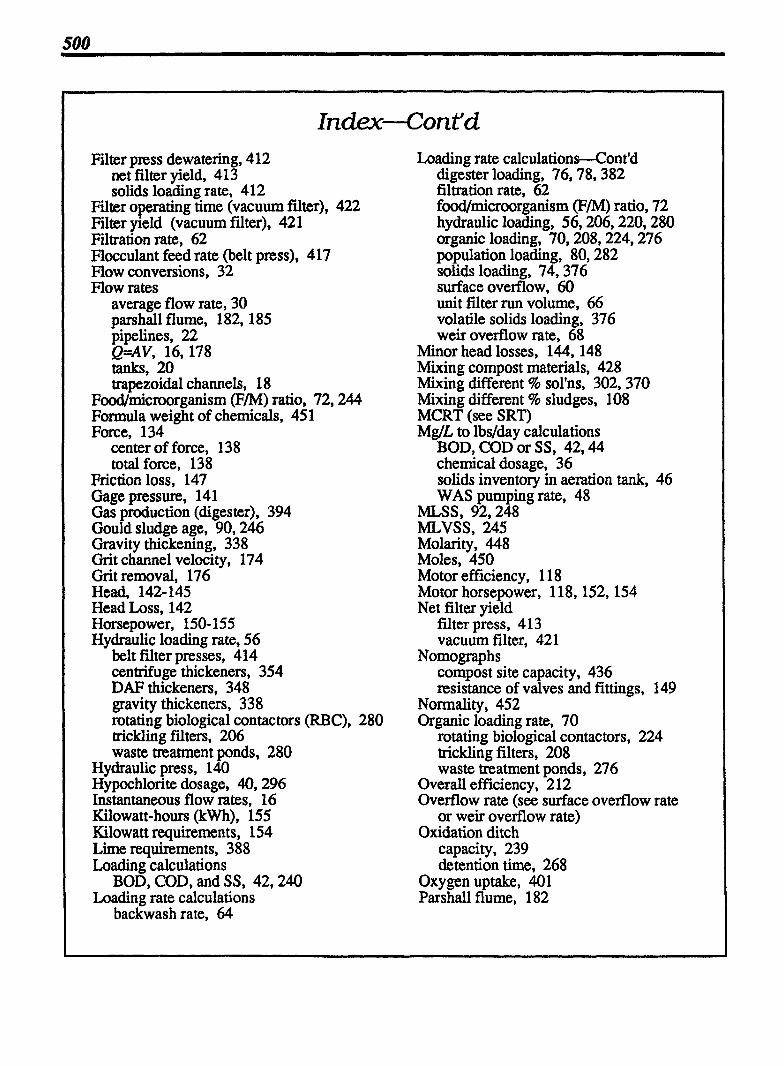
Filter press dewatering, 412 net film yield, 41 3 solids loading rate, 412
Filter operating time (vacuum fdter), 422 Filter yield (vacuum filter), 42 1 Filtration rate, 62 Flocculant feed rate (belt press), 417 mow conversions, 32 Flow rates
average flow rate, 30 parshall flume, 182,185 pipelines, 22 Q=AV, 16,178 tanks, 20 trapezoidal channels, 1 8
Food/micmrganism (F/M) ratio, 72,244 Formula weight of chemicals, 45 1 Force, 134
center of force, 138 total force, 138
Friction loss, 147 Gage pressure, 141 Gas production (digester), 394 Gould sludge age, 90,246 Gravity thickening, 338 Grit channel velocity, 174 Grit removal, 176 Head, 142- 145 Head Loss, 142 Horsepower, 150- 155 Hydraulic loading rate, 56
belt filter presses, 414 centrifuge thickeners, 354 DAF thickeners, 348 gravity thickeners, 33 8 rotating biological contactors (RBC), 280 trickling filters, 206 waste treatment ponds, 280
Hydraulic press, 140 Hypochlorite dosage, 40,296 Instantaneous flow rates, 16 Kilowatt-hours (kW), 155 Kilowatt requirements, 154 Lime requirements, 388 Loading calculations
BOD, COD, and SS, 42,240 Loading rate calculations
backwash rate, 64
Loading rate calculations-Cont'd digester loading, 76,78,382 filtration rate, 62 fOOd/microorganism (FM) ratio, 72 hydraulic loading, 56,206,220,280 organic loading, 70,208,224,276 population loading, 80,282 solids loading, 74,376 surface overflow, 60 unit filter run volume, 66 volatile solids loading, 376 weir overflow rate, 68
Minor head losses, 144,148 Mixing compost materials, 428 Mixing different % sol'ns, 302,370 Mixing different % sludges, 108 MCRT (see SRT) MgIL to lbs/da y calculations
BOD, COD or SS, 42,44 chemical dosage, 36 solids inventory in aeration tank, 46 WAS pumping rate, 48
MLSS, 92,248 MLVSS, 245 Molarity, 448 Moles, 450 Motor efficiency, 1 18 Motor horsepower, 1 18,152, 154 Net filter yield
filter press, 4 13 vacuum filter, 42 1
Nornographs compost site capacity, 436 resistance of valves and fittings, 149
Normality, 452 Organic loading rate, 70
rotating biological contactors, 224 trickling filters, 208 waste treatment ponds, 276
Overall efficiency, 212 Overflow rate (see surface overflow rate
or weir overflow rate) Oxidation ditch
capacity, 239 detention time, 268
Oxygen uptake, 401 Parshall flume, 182

Percent calculations, 99 recovery, 419,423 recycle rate, 352 seed sludge, 1 12 solids, 106,108,110,334 strength, 108,114,298,370 stroke setting, 308 volatile solids, 1 10 volatile solids reduction, 390
Plate and frame filter press (see filter press dewatering)
Population equivalent, 80,282 Population loading, 80,282 Positive displacement pumps, 160 Power, 150 Power costs, 155 Pressure, 141 psi, 137 Pumping
capacity, 156, 160 efficiency, 1 18 rate, 48, 11 1, 168,253,308,334
Q=AV, 16,174,178 RAS (see Return sludge rate) Recirculation ratio, 2 l4 Recycle rate, 352 Residual c hlorinc, 37 Return sludge rate, 254
using aeration tank solids balance, 258 using secondary clarifier solids bal., 256 using settleability, 254
Sand drying beds, 424 Screenings
pit capacity, 172 removed, 170
SDI, 468 Sedimentation, 1 87 Seed sludge, 112,378,380 Settleability , 456 Settleable solids, 458 Sludge
age, 90,246 blanket rise or fall, 346 density index, 468 digester storage, 384 feed rate, 415 pumping, 107,334,372 pump operating time, 374
Sludge-Cont'd thickening, 336 volume index, 466 withdrawal, 347,426
Solids balance, 344,396 inventory, 46,242 loading rate, 74,196,339,349,356,412,
416,420,425 percent, 44,106,198,210,334 retention time, 94,250 suspended, 464
Soluble BOD, 222 Solute, 114 Solutions
feeder calibration, 3 l4 mixing, 302,304 percent strength, 114,298,300
Solvent, 114 Specific gravity, 132, 137,154,301 SRT (see Solids, retention time) Suction lift and head, 142 Surface overflow rate, 60, 194 Suspended solids, 44,198,210,464 SVI, 466 Tank volumes, 238 Temperature, 470 Thickening, 336,338 Total dynamic head, 144 Total force, 138 Total solids, 460 Total suspended solids, 41 8 Triangular load, 139 Unit filter run volume, 66 Unit process efficiency, 104,200,210 Vacuum filer press dewatering
fdter loading, 420 filter operating time, 422 filter yield, 421 percent solids recovery, 423
Velocity grit channel, 174 using float or dye method, 27,175 using Q=AV, 26,174
Volatile acids/alkalinity ratio, 3 86 Volatile solids, 376,390,392,460,464 Volume, 1,4,6,8,9,238,239
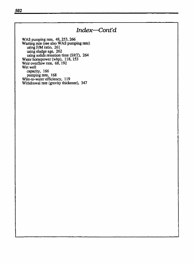
Index--Cont'd WAS pumping rate, 48,253,266 Wasting rate (see also WAS pumping rate)
using F/M ratio, 26 1 using sludge age, 262 using solids retention time (SW), 264
Water horsepower (whp), 1 18,153 Weir overflow rate, 68, 192 Wet well
capacity, 166 pumping rate, 168
Wire-to-water efficiency, 1 19 Withdrawal rate (gravity thickener), 347
Related Documents


