APPLICATIONS TO ECONOMICSsethi/Prosper/Control-Tex-Chapte11.pdf · APPLICATIONS TO ECONOMICS Optimal control theory has been extensively applied to the solution of economics problems

CHAPTER 11

APPLICATIONS TO ECONOMICS

Chapter 11 – p. 1/49

APPLICATIONS TO ECONOMICS

Optimal control theory has been extensively applied to the

solution of economics problems since the early papers that

appeared in Shell (1967) and the works of Arrow (1968)

and Shell (1969). The field is too vast to be surveyed in

detail here, however. Several books in the area are: Arrow

and Kurz (1970), Hadley and Kemp (1971), Takayama

(1974), Lesourne and Leban (1982), Seierstad and Sydsæter

(1987), Feichtinger (1988), Léonard and Long (1992), Van

Hilten, Kort, and Van Loon (1993), Kamien and Schwartz

(1998), and Dockner, Jørgensen, Long, and Sorger (2000).


11.1 MODELS OF OPTIMAL ECONOMIC GROWTH

The first model treated is a finite horizon fixed-end-pointmodel with stationary population. The problem is that ofmaximizing the present value of utility of consumption forsociety, and also accumulate a specified capital stock by theend of the horizon.

The second model incorporates an exogenously andexponentially growing population in the infinite horizonsetting. The method of phase diagrams is used to analyzethe model.

For related discussion and extensions of these models, seeArrow and Kurz (1970), Burmeister and Dobell (1970), andIntriligator (1971).


11.1.1 AN OPTIMAL CAPITAL ACCUMULATION MODEL

Consider a one-sector economy in which the stock ofcapital, denoted byK(t), is the only factor of production.Let F (K) be the output rate of the economy whenK is thecapital stock. AssumeF (0) = 0, F (K) > 0, F ′(K) > 0, andF ′′(K) < 0, for K > 0. The latter implies the diminishingmarginal productivity of capital. This output can either beconsumed or be reinvested for further accumulation ofcapital stock. LetC(t) be the amount of output allocated toconsumption, and letI(t) = F [K(t)] − C(t) be the amountinvested. Letδ be the constant rate of depreciation ofcapital. Then, the capital stock equation is

K = F (K) − C − δK, K(0) = K0. (1)


PROBLEM FORMULATION

Let U(C) be society’s utility of consumption, where weassumeU ′(0) = ∞, U ′(C) > 0, andU ′′(C) < 0, for C ≥ 0.Let ρ denote the social discount rate andT denote the finitehorizon. Then, a government which is elected for a term ofT years could consider the following problem:

max

{

J =

∫ T

0

e−ρtU [C(t)]dt

}

(2)

subject to (1) and the fixed-end-point condition

K(T ) = KT , (3)

whereKT is a given positive constant. It may be noted thatreplacing (3) byK(T ) ≥ KT would give the same solution.


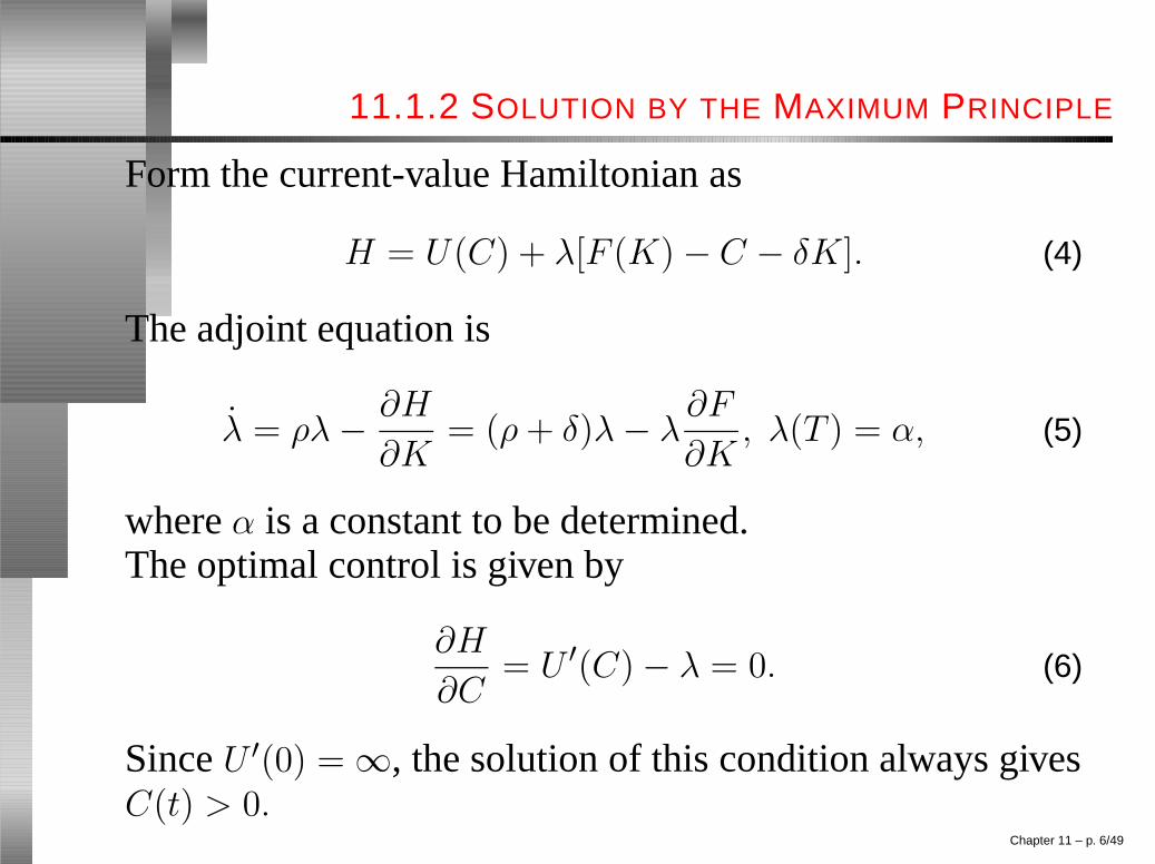
11.1.2 SOLUTION BY THE MAXIMUM PRINCIPLE

Form the current-value Hamiltonian as

H = U(C) + λ[F (K) − C − δK]. (4)

The adjoint equation is

λ = ρλ −∂H

∂K= (ρ + δ)λ − λ

∂F

∂K, λ(T ) = α, (5)

whereα is a constant to be determined.The optimal control is given by

∂H

∂C= U ′(C) − λ = 0. (6)

SinceU ′(0) = ∞, the solution of this condition always givesC(t) > 0.


SOLUTION BY THE MAXIMUM PRINCIPLE CONT.

The economic interpretation of the Hamiltonian is

straightforward: it consists of two terms, the first one gives

the utility of current consumption. The second term gives

the net investment evaluated by priceλ, which, from (6),

reflects the marginal utility of consumption.


CONDITIONS FOR OPTIMALITY

(a) The static efficiency condition (6) which maximizes thevalue of the Hamiltonian at each instant of time myopically,providedλ(t) is known.

(b) The dynamic efficiency condition (5) which forces thepriceλ of capital to change over time in such a way that thecapital stock always yields a net rate of return, which isequal to the social discount rateρ. That is,

dλ +∂H

∂Kdt = ρλdt.

(c) The long-run foresight condition, which establishes theterminal priceλ(T ) of capital in such a way that exactly theterminal capital stockKT is obtained atT .


SOLVING A TPBVP

Equations (1), (3), (5), and (6) form a two-point boundary

value problem which can be solved numerically. A

qualitative analysis of this system can also be carried out by

the phase diagram method of Chapter 7; see also Burmeister

and Dobell (1970). We do not give details here since a

similar analysis will be given for the infinite horizon version

of this model treated in Sections 11.1.3 and 11.1.4.

However, in Exercise 11.1 you are asked to solve a simple

version of the model in which the TPBVP can be solved

analytically.Chapter 11 – p. 9/49

10.1.3 A ONE-SECTOR MODEL

WITH A GROWING LABOR FORCE

We introduce a new factor labor (which for simplicity wetreat the same as the population), which is growingexponentially at a fixed rateg > 0. Let L(t) denote theamount of labor at timet. Then

L(t) = L(0)egt.

Let F (K,L) be the production function which is assumed tobe concave and homogeneous of degree one inK andL. Wedefinek = K/L and the per capita production functionf(k)

as

f(k) =F (K,L)

L= F (

K

L, 1) = F (k, 1). (7)

Chapter 11 – p. 10/49

THE STATE EQUATION

To derive the state equation fork, we note that

K = kL + kL = kL + kgL.

Substituting forK from (1) and defining per capita

consumptionc = C/L, we get

k = f(k) − c − γk, k(0) = k0, (8)

whereγ = g + δ.

Chapter 11 – p. 11/49

THE OBJECTIVE FUNCTION

Let u(c) be the utility of per capita consumption ofc, where

u is assumed to satisfy

u′(c) > 0 andu′′(c) < 0 for c > 0 andu′(0) = ∞. (9)

The objective is the total discounted per capita consumption

utilities over time. Thus, we

maximize{

J =

∫

∞

0

e−ρtu(c)dt

}

. (10)

Note that the optimal control model defined by (8) and (10)

is a generalization of Exercise 3.6.Chapter 11 – p. 12/49


The current-value Hamiltonian is

H = u(c) + λ[f(k) − c − γk]. (11)

The adjoint equation is

λ = ρλ −∂H

∂k= (ρ + γ)λ − f ′(k)λ. (12)

To obtain the optimal control, we differentiate (11) withrespect toc, set it to zero, and solve

u′(c) = λ. (13)

Let c = h(λ) = u′−1(λ) denote the solution of (13).

Chapter 11 – p. 13/49


To show that the maximum principle is sufficient for

optimality we will show that the derived Hamiltonian

H0(k, λ) is concave ink for anyλ solving (13); see Exercise

11.2. However, this follows immediately from the facts that

u′(c) is positive as assumed in (9) and thatf(k) is concave

because of the assumptions onF (K,L).

Equations (8), (12), and (13) now constitute a complete

autonomous system, since time does not enter explicitly in

these equations. Therefore, we can use the phase diagram

solution technique employed in Chapter 7.Chapter 11 – p. 14/49

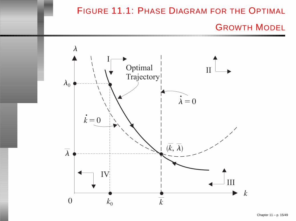
FIGURE 11.1: PHASE DIAGRAM FOR THE OPTIMAL

GROWTH MODEL

Chapter 11 – p. 15/49

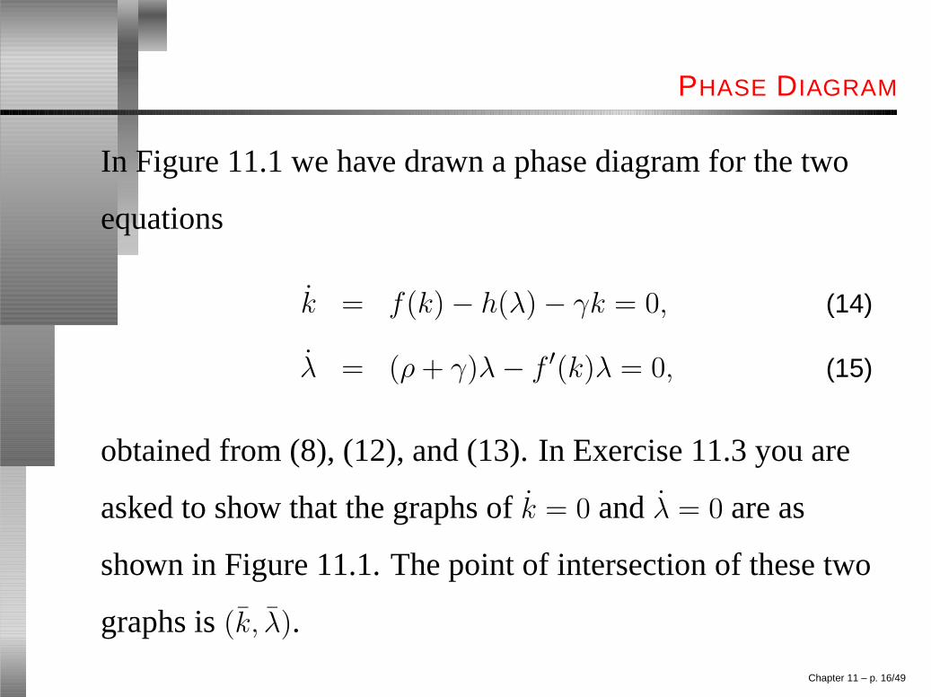
PHASE DIAGRAM

In Figure 11.1 we have drawn a phase diagram for the two

equations

k = f(k) − h(λ) − γk = 0, (14)

λ = (ρ + γ)λ − f ′(k)λ = 0, (15)

obtained from (8), (12), and (13). In Exercise 11.3 you are

asked to show that the graphs ofk = 0 andλ = 0 are as

shown in Figure 11.1. The point of intersection of these two

graphs is(k, λ).

Chapter 11 – p. 16/49

PHASE DIAGRAM CONT.

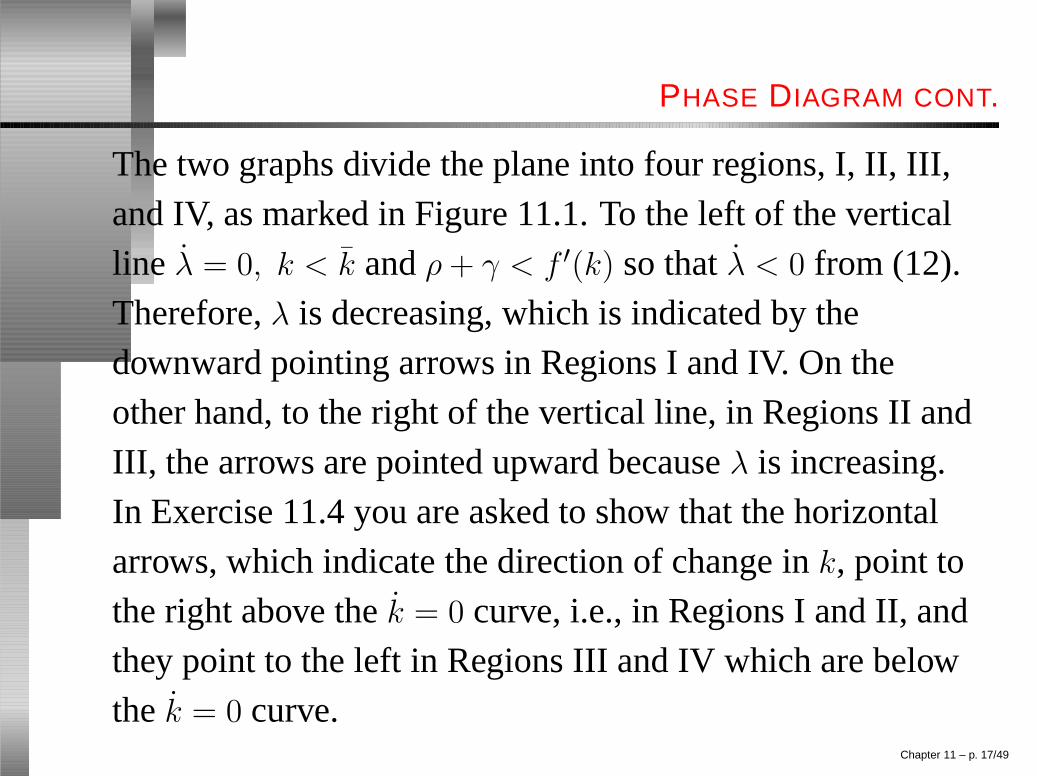
The two graphs divide the plane into four regions, I, II, III,and IV, as marked in Figure 11.1. To the left of the verticalline λ = 0, k < k andρ + γ < f ′(k) so thatλ < 0 from (12).Therefore,λ is decreasing, which is indicated by thedownward pointing arrows in Regions I and IV. On theother hand, to the right of the vertical line, in Regions II andIII, the arrows are pointed upward becauseλ is increasing.In Exercise 11.4 you are asked to show that the horizontalarrows, which indicate the direction of change ink, point tothe right above thek = 0 curve, i.e., in Regions I and II, andthey point to the left in Regions III and IV which are belowthe k = 0 curve.

Chapter 11 – p. 17/49

PHASE DIAGRAM CONT.

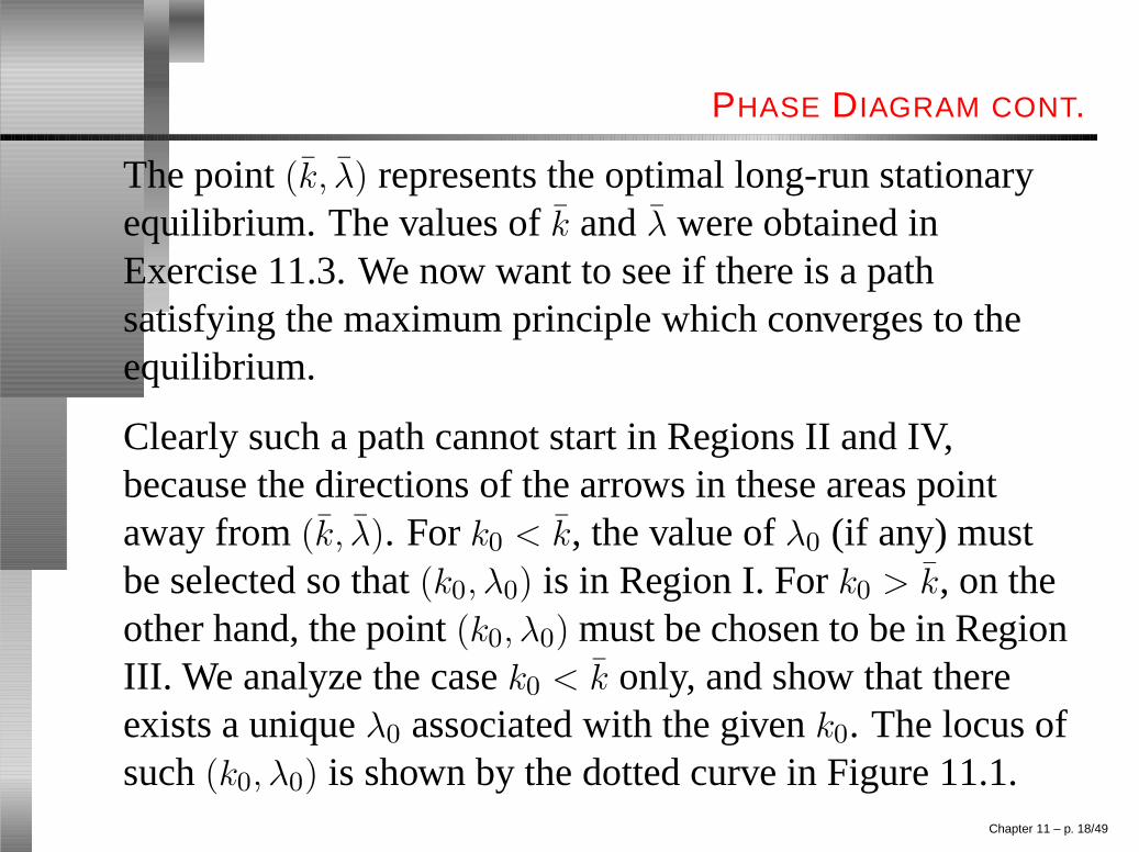
The point(k, λ) represents the optimal long-run stationaryequilibrium. The values ofk andλ were obtained inExercise 11.3. We now want to see if there is a pathsatisfying the maximum principle which converges to theequilibrium.

Clearly such a path cannot start in Regions II and IV,because the directions of the arrows in these areas pointaway from(k, λ). Fork0 < k, the value ofλ0 (if any) mustbe selected so that(k0, λ0) is in Region I. Fork0 > k, on theother hand, the point(k0, λ0) must be chosen to be in RegionIII. We analyze the casek0 < k only, and show that thereexists a uniqueλ0 associated with the givenk0. The locus ofsuch(k0, λ0) is shown by the dotted curve in Figure 11.1.

Chapter 11 – p. 18/49

PHASE DIAGRAM CONT.

In Region I,k(t) is an increasing function oft as indicated

by the horizontal right-directed arrow. Therefore, we can

replace the independent variablet by k as below, and then

use (14) and (15) to obtain

d(ln λ)

dk=

[

1

λ

dλ

dt

] /

dk

dt=

f ′(k) − (ρ + γ)

h(λ) + γk − f(k). (16)

Fork < k, the right-hand side of (16) is negative, and since

h(λ) decreases asλ increases, we haved(ln λ)/dk increasing

with λ.

Chapter 11 – p. 19/49

UNIQUENESS OF THE CONVERGENCE PATH

We show next that there can be at most one trajectory for aninitial capitalk0 < k. Assume to the contrary thatλ1(k) andλ2(k) are two paths leading to(k, λ) and are such that theselected initial values satisfyλ1(k0) > λ2(k0) > 0. Sinced(lnλ)/dk increases withλ,

d ln[λ1(k)/λ2(k)]

dk=

d ln λ1(k)

dk−

d ln λ2(k)

dk> 0,

wheneverλ1(k) > λ2(k). This inequality clearly holds atk0,and by (16),λ1(k)/λ2(k) increases atk0. This in turnimplies that the inequality holds atk0 + ε, whereε > 0 issmall. Now replacek0 by k0 + ε and repeat the argument.Thus, the ratioλ1(k)/λ2(k) increases ask increases so thatλ1(k) andλ2(k) cannot both converge toλ ask → k.

Chapter 11 – p. 20/49

EXISTENCE OF A CONVERGENCE PATH

To show that fork0 < k, there exists aλ0 such that the

trajectory converges to(k, λ), note that for some starting

values of the adjoint variable, the resulting trajectory(k, λ)

enters Region II and then diverges, while for others it enters

Region IV and diverges. By continuity, there exists a

starting valueλ0 such that the resulting trajectory(k, λ)

converges to(k, λ).

Similar arguments hold for the casek0 > k, which we

therefore omit.

Chapter 11 – p. 21/49

11.2 A MODEL OF OPTIMAL EPIDEMIC CONTROL

Certain infectious epidemic diseases are seasonal in nature.

Examples are the common cold, flu, and certain children’s

diseases. When it is beneficial to do so, control measures

are taken to alleviate the effects of these diseases. Here we

discuss a simple control model due to Sethi (1974c) for

analyzing the epidemic problem. Related problems have

been treated by Sethi and Staats (1978), Sethi (1978d), and

Francis (1997). See Wickwire (1977) for a good survey of

optimal control theory applied to the control of pest

infestations and epidemics, and Swan (1984) for

applications to biomedicine.Chapter 11 – p. 22/49

11.2.1 FORMULATION OF THE MODEL

Let N be the total fixed population. Letx(t) be the numberof infectives at timet so that the remainingN − x(t) is thenumber of susceptibles. Assume that no immunity isacquired so that when infected people are cured, theybecome susceptible again. The state equation governing thedynamics of the epidemic spread in the population is

x = βx(N − x) − vx, x(0) = x0, (17)

whereβ is a positive constant termedinfectivity of thedisease, andv is a control variable reflecting the level ofmedical program effort. Note thatx(t) is in [0, N ] for allt > 0 if x0 is in that interval.

Chapter 11 – p. 23/49

FORMULATION OF THE MODEL CONT.

The objective of the control problem is to minimize thepresent value of the cost stream up to a horizon timeT ,which marks the end of the season for that disease. LetCdenote the unit social cost per infective, letK denote thecost of control per unit level of program effort, and letQdenote the capability of the health care delivery systemproviding an upper bound onv. The optimal controlproblem is:

max

{

J =

∫ T

0

−(Cx + Kv)e−ρtdt

}

(18)

subject to (17), the terminal constraint thatx(T ) = xT , (19)

and the control constraint0 ≤ v ≤ Q.

Chapter 11 – p. 24/49

11.2.2 SOLUTION BY GREEN’S THEOREM

Rewriting (17) as

vdt = [βx(N − x)dt − dx]/x

and substituting into (18) yields the line integral

JΓ =

∫

Γ

−

{

[Cx + Kβ(N − x)]e−ρtdt −K

xe−ρtdx

}

, (20)

whereΓ is a path fromx0 to xT in the(t, x)-space.

Chapter 11 – p. 25/49

SOLUTION BY GREEN’S THEOREM CONT.

Let Γ1 andΓ2 be two such paths fromx0 to xT , and letR be

the region enclosed byΓ1 andΓ2. By Green’s theorem, we

can write

JΓ1−Γ2= JΓ1

− JΓ2=

∫ ∫

R

−

[

kρ

x− C + Kβ

]

e−ρtdtdx.

(21)

To obtain the singular control we set the integrand of (21)

equal to zero, as we did in Chapter 7. This yields

x =ρ

c/K − β=

ρ

θ, (22)

whereθ = C/K − β.

Chapter 11 – p. 26/49


Define the singular statexs as follows:

xs =

{

ρ/θ if 0 < ρ/θ < N,

N otherwise.(23)

The corresponding singular control level

vs = β(N − xs) =

{

β(N − ρ/θ) if 0 < ρ/θ < N,

0 otherwise.(24)

We will show thatxs is the turnpike level of infectives. It isinstructive to interpret (23) and (24) for the various cases. Ifρ/θ > 0, thenθ > 0 so thatC/K > β. Here the smaller theratioC/K, the larger the turnpike levelxs, and therefore,the smaller the medical program effort should be.

Chapter 11 – p. 27/49


Whenρ/θ < 0, you are asked to show in Exercise 11.6 that

xs = N in the caseC/K < β, which means the ratio of the

social cost to the treatment cost is smaller than the

infectivity coefficient. Therefore, in this case when thereis

no terminal constraint, the optimal trajectory involves no

treatment effort. An example of this case is the common

cold where the social cost is low and treatment cost is high.

Chapter 11 – p. 28/49


• The optimal control for the fortuitous case when

xT = xs is

v∗(x(t)) =

Q if x(t) > xs,

vs if x(t) = xs,

0 if x(t) < xs.

(25)

• WhenxT 6= xs, there are two cases to consider. For

simplicity of exposition we assumex0 > xs andT and

Q to be large.

(1) xT > xs: See Figure 11.2.

(2) xT < xs: See Figure 11.3. It can be shown thatx

goes asymptotically toN − Q/β if v = Q.

Chapter 11 – p. 29/49

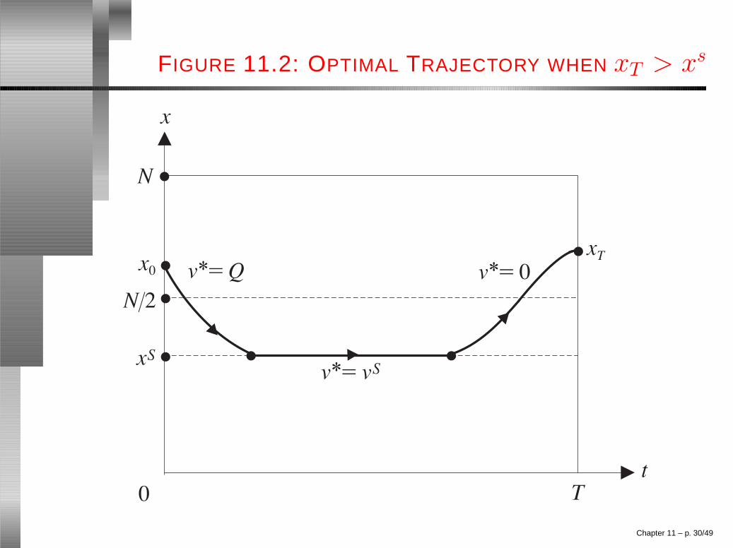
FIGURE 11.2: OPTIMAL TRAJECTORY WHEN xT > xs

Chapter 11 – p. 30/49

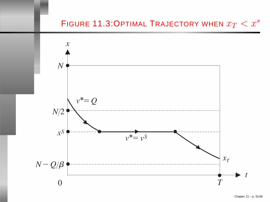
FIGURE 11.3:OPTIMAL TRAJECTORY WHEN xT < xs

Chapter 11 – p. 31/49

11.3 A POLLUTION CONTROL MODEL

We describe a simple pollution control model due to Keeler,

Spence, and Zeckhauser (1971). We shall describe this

model in terms of an economic system in which labor is the

only primary factor of production, which is allocated

between food production and DDT production. Once

produced (and used) DDT is a pollutant which can only be

reduced by natural decay. However, DDT is a secondary

factor of production which, along with labor, determines the

food output. The objective of the society is to maximize the

total present value of the utility of food less the disutility of

pollution due to the DDT use.

Chapter 11 – p. 32/49

11.3.1 MODEL FORMULATION

We introduce the following notation:

b = the total labor force, assumed to be constant forsimplicity,

v = the amount of labor used for DDT production,

b − v = the amount of labor used for food production,

P = the stock of pollution at timet,

a(v) = the rate of DDT output;a(0) = 0, a′ > 0, a′′ < 0,for v ≥ 0,

δ = the natural exponential decay rate of DDT pollu-tion,

Chapter 11 – p. 33/49

NOTATION CONT.

C(v) = f [b − v, a(v)] = the rate of food output;C(v) isconcave,C(0) > 0, C(b) = 0; C(v) attains aunique maximum atv = V > 0; see Figure 11.4.Note that a sufficient condition forC(v) to bestrictly concave isf12 ≥ 0 along with the usualconcavity and monotonicity conditions onf ,

g(C) = the utility of consumption;g′(0) = ∞, g′ ≥ 0,

g′′ < 0,

h(P ) = the disutility of pollution; h′(0) = 0, h′ ≥

0, h′′ > 0.

Chapter 11 – p. 34/49

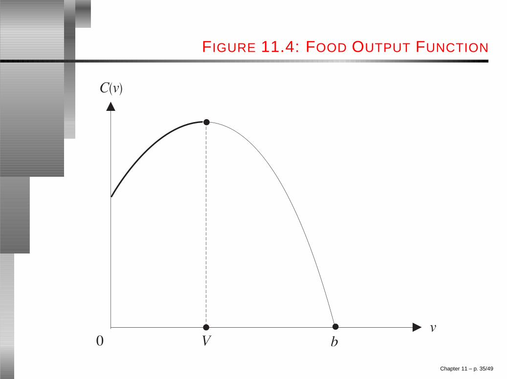
FIGURE 11.4: FOOD OUTPUT FUNCTION

Chapter 11 – p. 35/49

PROBLEM FORMULATION

The optimal control problem is:

max

{

J =

∫

∞

0

e−ρt[g(C(v)) − h(P )]dt

}

(26)

subject toP = a(v) − δP, P (0) = P0, (27)

0 ≤ v ≤ b. (28)

From Figure 11.4 it is obvious thatv is at mostV , since theproduction of DDT beyond that level decreases foodproduction as well as increases DDT pollution. Hence, (28)can be reduced to simply

v ≥ 0. (29)

Chapter 11 – p. 36/49


Form the current-value Lagrangian

L(P, v, λ, µ) = g[C(v)] − h(P ) + λ[a(v) − δP ] + µv (30)

using (26), (27) and (29), where

λ = (ρ + δ)λ + h′(P ), (31)

and

µ ≥ 0 and µv = 0. (32)

The optimal solution is given by

∂L

∂v= g′[C(v)]C ′(v) + λa′(v) + µ = 0. (33)

Chapter 11 – p. 37/49


Since the derived Hamiltonian is concave, conditions

(30)-(33) together with

limt→∞

λ(t) = λ = constant (34)

are sufficient for optimality; see Theorem 2.1 and Section

2.4. The phase diagram analysis presented below givesλ(t)

satisfying (34).

Chapter 11 – p. 38/49

11.3.3 PHASE DIAGRAM ANALYSIS

Sinceh′(0) = 0, g′(0) = ∞, andv > 0, it pays to producesome positive amount of DDT in equilibrium. Therefore,the equilibrium value of the Lagrange multiplier is zero, i.e.,µ = 0. From (27), (31) and (33), we get the equilibriumvaluesP , λ, andv as follows:

P =a(v)

δ, (35)

λ = −h′(P )

ρ + δ= −

g′[C(v)]C ′(v)

a′(v). (36)

From (36) and the assumptions on the derivatives ofg, C

anda, we know thatλ < 0. From this and (31), we concludethatλ(t) is always negative.

Chapter 11 – p. 39/49

PHASE DIAGRAM ANALYSIS CONT.

The economic interpretation ofλ is that−λ is the imputedcost of pollution. Letv = Φ(λ) denote the solution of (33)with µ = 0. On account of (29), define

v∗ = max[0,Φ(λ)]. (37)

We know from the interpretation ofλ that whenλ increases,the imputed cost of pollution decreases, which can justifyan increase in the DDT production to ensure an increasedfood output. Thus, it is reasonable to assume that

dΦ

dλ> 0,

and we will make this assumption. It follows that thereexists a uniqueλc such thatΦ(λc) = 0, Φ(λ) < 0 for λ < λc

andΦ(λ) > 0 for λ > λc.Chapter 11 – p. 40/49

DIAGRAM ANALYSIS CONT.

To construct the phase diagram, we must plotP = 0 andλ = 0. These are

P =a(v∗)

δ=

a[max{0,Φ(λ)}]

δ, (38)

h′(P ) = −(ρ + δ)λ. (39)

Observe that the assumptionh′(0) = 0 implies that the graphof (39) passes through the origin. Differentiating theseequations with respect toλ and using (37), we obtain

dP

dλ=

a′(v)

δ

dv

dλ> 0 (40)

anddP

dλ= −

(ρ + δ)

h′′(P )< 0. (41)

Chapter 11 – p. 41/49


The intersection point(λ, P ) of the curves (38) and (39)denotes the equilibrium levels for the adjoint variable andthe pollution stock, respectively. From arguments similartothose in Section 11.1.4, it can be shown that there exists anoptimal path (shown dotted in Figure 11.5) converging tothe equilibrium(λ, P ).

Givenλc as the intersection of theP = 0 curve and thehorizontal axis, the corresponding ordinateP c on theoptimal trajectory is the related pollution stock level. Thesignificance ofP c is that if the existing pollution stockP islarger thanP c, then the optimal control isv∗ = 0, meaningno DDT is produced.

Chapter 11 – p. 42/49

FIGURE 11.5: PHASE DIAGRAM FOR THE POLLUTION

CONTROL MODEL

Chapter 11 – p. 43/49


Given an initial level of pollutionP0, the optimal trajectorycurve in Figure 11.5 provides the initial valueλ0 of theadjoint variable. With these initial values, the optimaltrajectory is determined by (27), (31), and (37). IfP0 > P c,thenv∗ = 0 until such time that the natural decay ofpollution stock has reduced it toP c. At that time the adjointvariable has increased to the valueλc. The optimal controlis v∗ = φ(λ) from this time on, and the path converges to(λ, P ).

At equilibrium, v = Φ(λ) > 0, which implies that it isoptimal to produce some DDT forever in the long run. Theonly time when its production is not optimal is at thebeginning when the pollution stock is higher thanP c.

Chapter 11 – p. 44/49


It is important to examine the effects of changes in the

parameters on the optimal path. In particular, you are asked

in Exercise 11.7 to show that an increase in the natural rate

of decay of pollution,δ, will increaseP c. That is, the higher

is the rate of decay, the higher is the level of pollution stock

at which the pollutant’s production is banned. For DDT,δ is

small so that its complete ban, which has actually occurred,

may not be far from the optimal policy.

Chapter 11 – p. 45/49

11.4 MISCELLANEOUS APPLICATIONS

Control theory applications to economics:

• Optimal educational investments.

• Limit pricing and uncertain entry.

• Adjustment costs in the theory of competitive firms.

• International trade.

• Money demand with transaction costs.

• Design of an optimal insurance policy.

• Optimal training and heterogeneous labor.

• Population policy.

Chapter 11 – p. 46/49

MISCELLANEOUS APPLICATIONS CONT.

Control theory applications to economics (cont):

• Optimal income tax.

• Continuous expanding economies.

• Investment and marketing policies in a duopoly.

• Theory of firm under government regulations.

• Renumeration patterns for medical services.

• Dynamic shareholder behavior under personal taxation.

• Optimal input substitution in response to environmentalconstraints.

• Optimal crackdowns on a drug market.Chapter 11 – p. 47/49


Applications to management science and operationsresearch:

• Labor assignments.

• Distribution and transportation applications.

• Scheduling and network planning problems.

• Research and development.

• City congestion problems.

• Warfare models.

• National settlement planning.

• Pricing with dynamic demand and production costs.

• Accelerating diffusion of innovation.Chapter 11 – p. 48/49


Applications to management science and operationsresearch (cont):

• Optimal acquisition of new technology.

• Optimal pricing and/or advertising for monopolisticdiffusion model.

• Manpower planning.

• Optimal quality and advertising under asymmetricinformation.

• Optimal recycling of tailings for production of buildingmaterials.

• Planning for information technology.

Chapter 11 – p. 49/49

APPLICATIONS TO ECONOMICSsethi/Prosper/Control-Tex-Chapte11.pdf · APPLICATIONS TO ECONOMICS Optimal control theory has been extensively applied to the solution of economics problems

Documents