APPLICATIONS OF SYNCHROTRON RADIATION TECHNIQUES TO THE STUDY OF TAPHONOMIC ALTERATIONS AND PRESERVATION IN FOSSILS A Thesis Submitted to the Faculty of Graduate Studies and Research In Partial Fulfillment of the Requirements For the Degree of Doctor of Philosophy in Physics University of Regina by Anezka Popovski Kolaceke Regina, Saskatchewan February, 2019 Copyright 2019: A. P. Kolaceke

Welcome message from author
This document is posted to help you gain knowledge. Please leave a comment to let me know what you think about it! Share it to your friends and learn new things together.
Transcript

APPLICATIONS OF SYNCHROTRON RADIATION TECHNIQUES TO THE STUDY OF TAPHONOMIC ALTERATIONS AND PRESERVATION IN FOSSILS
A Thesis
Submitted to the Faculty of Graduate Studies and Research
In Partial Fulfillment of the Requirements
For the Degree of
Doctor of Philosophy
in
Physics
University of Regina
by
Anezka Popovski Kolaceke
Regina, Saskatchewan
February, 2019
Copyright 2019: A. P. Kolaceke
UNIVERSITY OF REGINA
FACULTY OF GRADUATE STUDIES AND RESEARCH
SUPERVISORY AND EXAMINING COMMITTEE
Anezka Popovski Kolaceke, candidate for the degree of Doctor of Philosophy in Physics, has presented a thesis titled, Applications of Synchrotron Radiation Techniques to the Study of Taphonomic Alterations and Preservations in Fossils, in an oral examination held on December 21, 2018. The following committee members have found the thesis acceptable in form and content, and that the candidate demonstrated satisfactory knowledge of the subject material. External Examiner: *Dr. Phil Bell, University of New England
Co-Supervisor: Dr. Mauricio Barbi, Department of Physics
Co-Supervisor: Dr. Ryan McKellar, Department of Physics
Committee Member: Dr. Josef Buttigieg, Department of Biology
Committee Member: **Dr. Maria Velez Caicedo, Department of Geology
Committee Member: Dr. Garth Huber, Department of Physics
Chair of Defense: Dr. Fanhua Zeng, Faclty of Graduate Studies & Research *via ZOOM Conferencing **Not present at defense

Abstract
Fossils have traditionally been seen as sedimentary rocks that preserve little of the
original composition of animals, except for their shapes, and perhaps some original
material from recalcitant mineralized structures, such as bones, and teeth. However,
recent studies have shown that not the case. Researchers have identified preserved
organic molecules, such as collagen and melanosomes, as well as mineralized soft
tissues, including feathers, muscle tissue and skin, tens of millions of years after the
animal’s death. These results have improved our understanding of extinct species,
and have been obtained using a variety of characterization techniques, including the
synchrotron-based approaches that are the focus of the research presented in this
thesis. The main goal of the research discussed in this thesis was the application of
synchrotron radiation techniques (X-ray fluorescence and X-ray absorption
spectroscopy, in particular) in order to determine the taphonomic alterations that
fossils experience, and examine how different materials are preserved.
In this thesis, I discuss the results of the chemical characterization on the
remains of the Tyrannosaurus rex known as “Scotty”, turtle shells, and a rare
specimen of fossilized hadrosaur skin. I also examine the applicability of X-ray
fluorescence to determine the composition and elemental distribution of insect
inclusions in amber. The results presented herein offer possible explanations on how
some of these specimens were preserved and the extent of the chemical alterations
they underwent during their taphonomic history.
Beyond the specific results for each specimen, the overall research presented in
this thesis shows that synchrotron radiation techniques have great potential to
advance palaeontological research, as it becomes necessary to evaluate the chemistry
of specimens in high resolution. These characterization techniques were able to
confirm that more original material is preserved after fossilization than would have
been believed possibly even a decade ago.
i

Acknowledgements
I would like to thank my supervisors, Mauricio Barbi and Ryan McKellar, for all the
help and advice during the development of this project, for the suggestions and
corrections on this thesis, and for all other learning opportunities I was offered. I
would also like to thank the members of my Ph. D. committee for all the
suggestions and comments throughout the last years. All the help and discussions
were fundamental for the development of this thesis.
I am grateful for the support from the Physics Department at the University of
Regina and all faculty members, students and staff, and the Faculty of Graduate
Studies and Research for the funding through a Graduate Research Fellowship,
teaching assistantships and other scholarships and awards I received during my
studies. I would also like to thank all the Royal Saskatchewan Museum staff who
helped in the selection and preparation of samples and received me so well every
time I visited, specially Wes Long.
The research described in this thesis was performed at the Canadian Light Source.
I would like to thank all the beamline scientists and CLS staff that were always so
helpful and friendly. I also acknowledge the receipt of support from the CLS Graduate
Student Travel Support Program.
I thank all the researchers that co-authored manuscripts with me for this research,
including Maria Velez, Ian Coulson, Tim Tokaryk, and my supervisors. I am also
grateful to all the comments by reviewers and editors from the submitted papers.
Finally, I would like to express my gratitude to my family and friends for their
patience and emotional support. You are part of the reason I was able to finish this
thesis.
ii
Contents
Contents iii
List of Tables viii
List of Figures ix
1 Introduction and thesis structure 1
2 Taphonomy 4
2.1 Abstract . . . . . . . . . . . . . . . . . . . . . . . . . . . . . . . . . . 4
2.2 Introduction . . . . . . . . . . . . . . . . . . . . . . . . . . . . . . . . 4
2.3 Taphonomy of vertebrates . . . . . . . . . . . . . . . . . . . . . . . . 5
2.3.1 Decay . . . . . . . . . . . . . . . . . . . . . . . . . . . . . . . 5
2.3.2 Physical processes . . . . . . . . . . . . . . . . . . . . . . . . . 6
Weathering . . . . . . . . . . . . . . . . . . . . . . . . . . . . 6
Transport . . . . . . . . . . . . . . . . . . . . . . . . . . . . . 8
Time-Averaging . . . . . . . . . . . . . . . . . . . . . . . . . . 12
Bioturbation . . . . . . . . . . . . . . . . . . . . . . . . . . . . 13
2.3.3 Chemical processes . . . . . . . . . . . . . . . . . . . . . . . . 14
Silicification . . . . . . . . . . . . . . . . . . . . . . . . . . . . 14
Pyritization . . . . . . . . . . . . . . . . . . . . . . . . . . . . 15
Phosphatization . . . . . . . . . . . . . . . . . . . . . . . . . . 17
2.4 Preservation in vertebrates . . . . . . . . . . . . . . . . . . . . . . . . 18
2.4.1 Bones . . . . . . . . . . . . . . . . . . . . . . . . . . . . . . . 18
2.4.2 Soft-tissues . . . . . . . . . . . . . . . . . . . . . . . . . . . . 19
2.4.3 Integument . . . . . . . . . . . . . . . . . . . . . . . . . . . . 20
2.5 Special preservation . . . . . . . . . . . . . . . . . . . . . . . . . . . . 22
iii

2.5.1 Konzentrat-Lagerstatten . . . . . . . . . . . . . . . . . . . . . 23
2.5.2 Konservat-Lagerstatten . . . . . . . . . . . . . . . . . . . . . . 23
Preservation in amber . . . . . . . . . . . . . . . . . . . . . . 25
2.6 Conclusions . . . . . . . . . . . . . . . . . . . . . . . . . . . . . . . . 29
3 Synchrotron light sources and techniques 31
3.1 Abstract . . . . . . . . . . . . . . . . . . . . . . . . . . . . . . . . . . 31
3.2 Introduction . . . . . . . . . . . . . . . . . . . . . . . . . . . . . . . . 31
3.3 Synchrotron light sources . . . . . . . . . . . . . . . . . . . . . . . . . 33
3.3.1 Acceleration . . . . . . . . . . . . . . . . . . . . . . . . . . . . 33
3.3.2 Beam focusing . . . . . . . . . . . . . . . . . . . . . . . . . . . 36
3.3.3 Generating radiation . . . . . . . . . . . . . . . . . . . . . . . 37
3.4 X-ray fluorescence (XRF) . . . . . . . . . . . . . . . . . . . . . . . . 40
3.4.1 Theory and techniques . . . . . . . . . . . . . . . . . . . . . . 40
Spatially resolved XRF . . . . . . . . . . . . . . . . . . . . . . 41
XRF mapping . . . . . . . . . . . . . . . . . . . . . . . . . . . 42
3.4.2 Quantitative analysis . . . . . . . . . . . . . . . . . . . . . . . 44
3.5 X-ray absorption fine structure (XAFS) . . . . . . . . . . . . . . . . . 46
3.5.1 The XANES spectra . . . . . . . . . . . . . . . . . . . . . . . 48
Edge . . . . . . . . . . . . . . . . . . . . . . . . . . . . . . . . 49
Pre-edge . . . . . . . . . . . . . . . . . . . . . . . . . . . . . . 49
Post-edge . . . . . . . . . . . . . . . . . . . . . . . . . . . . . 50
3.5.2 Qualitative and semi-quantitative analysis . . . . . . . . . . . 50
Edge shift . . . . . . . . . . . . . . . . . . . . . . . . . . . . . 50
Linear combination analysis (LCA) . . . . . . . . . . . . . . . 50
Principal component analysis (PCA) . . . . . . . . . . . . . . 51
Deconvolution of XANES features . . . . . . . . . . . . . . . . 51
3.5.3 Quantitative analysis . . . . . . . . . . . . . . . . . . . . . . . 51
iv
Theory . . . . . . . . . . . . . . . . . . . . . . . . . . . . . . . 51
Analysis options . . . . . . . . . . . . . . . . . . . . . . . . . . 54
3.6 Conclusions . . . . . . . . . . . . . . . . . . . . . . . . . . . . . . . . 56
4 Chemical diagenesis of Tyrannosaurus rex bones from the
Frenchman Formation 58
4.1 Abstract . . . . . . . . . . . . . . . . . . . . . . . . . . . . . . . . . . 58
4.2 Introduction . . . . . . . . . . . . . . . . . . . . . . . . . . . . . . . 59
4.2.1 Scotty, the Saskatchewan T. rex . . . . . . . . . . . . . . . . . 63
4.3 Material and methods . . . . . . . . . . . . . . . . . . . . . . . . . . 65
4.4 Results . . . . . . . . . . . . . . . . . . . . . . . . . . . . . . . . . . 67
4.5 Discussion . . . . . . . . . . . . . . . . . . . . . . . . . . . . . . . . . 75
4.6 Conclusions . . . . . . . . . . . . . . . . . . . . . . . . . . . . . . . . 79
5 Non-destructive chemical analysis of insect inclusions in amber 81
5.1 Abstract . . . . . . . . . . . . . . . . . . . . . . . . . . . . . . . . . . 81
5.2 Introduction . . . . . . . . . . . . . . . . . . . . . . . . . . . . . . . . 82
5.3 Material and methods . . . . . . . . . . . . . . . . . . . . . . . . . . 86
5.3.1 Specimens and preparation . . . . . . . . . . . . . . . . . . . . 86
5.3.2 Measurements and analyses . . . . . . . . . . . . . . . . . . . 88
5.4 Results . . . . . . . . . . . . . . . . . . . . . . . . . . . . . . . . . . . 91
5.4.1 XRF applied to insect inclusions . . . . . . . . . . . . . . . . . 91
5.4.2 Preservation of ant inclusions in Baltic amber . . . . . . . . . 95
5.5 Discussion . . . . . . . . . . . . . . . . . . . . . . . . . . . . . . . . . 102
5.5.1 XRF applied to insect inclusions . . . . . . . . . . . . . . . . 102
Modern ants . . . . . . . . . . . . . . . . . . . . . . . . . . . . 102
Baltic amber . . . . . . . . . . . . . . . . . . . . . . . . . . . 103
North Carolina amber . . . . . . . . . . . . . . . . . . . . . . 105
v

5.5.2 Preservation of ant inclusions in Baltic amber . . . . . . . . . 106
5.6 Conclusions . . . . . . . . . . . . . . . . . . . . . . . . . . . . . . . . 109
6 Chemical diagenesis of turtle shells 112
6.1 Abstract . . . . . . . . . . . . . . . . . . . . . . . . . . . . . . . . . . 112
6.2 Introduction . . . . . . . . . . . . . . . . . . . . . . . . . . . . . . . . 113
6.3 Material and methods . . . . . . . . . . . . . . . . . . . . . . . . . . 115
6.4 Results . . . . . . . . . . . . . . . . . . . . . . . . . . . . . . . . . . 117
6.5 Discussion . . . . . . . . . . . . . . . . . . . . . . . . . . . . . . . . . 127
6.6 Conclusions . . . . . . . . . . . . . . . . . . . . . . . . . . . . . . . . 132
7 Chemical diagenesis of individual structures in hadrosaurid skin
layer 134
7.1 Abstract . . . . . . . . . . . . . . . . . . . . . . . . . . . . . . . . . . 134
7.2 Introduction . . . . . . . . . . . . . . . . . . . . . . . . . . . . . . . . 135
7.3 Material and methods . . . . . . . . . . . . . . . . . . . . . . . . . . 138
7.3.1 Specimen and geological settings . . . . . . . . . . . . . . . . 138
7.3.2 Methodology . . . . . . . . . . . . . . . . . . . . . . . . . . . 139
7.4 Results . . . . . . . . . . . . . . . . . . . . . . . . . . . . . . . . . . 142
7.5 Discussion . . . . . . . . . . . . . . . . . . . . . . . . . . . . . . . . . 150
7.6 Conclusions . . . . . . . . . . . . . . . . . . . . . . . . . . . . . . . . 154
8 Synchrotron applied to taphonomic studies 155
8.1 Abstract . . . . . . . . . . . . . . . . . . . . . . . . . . . . . . . . . . 155
8.2 Introduction . . . . . . . . . . . . . . . . . . . . . . . . . . . . . . . . 155
8.3 Results . . . . . . . . . . . . . . . . . . . . . . . . . . . . . . . . . . . 155
8.4 Discussion . . . . . . . . . . . . . . . . . . . . . . . . . . . . . . . . . 163
8.4.1 Relative concentrations . . . . . . . . . . . . . . . . . . . . . . 163
8.4.2 Correlation plots . . . . . . . . . . . . . . . . . . . . . . . . . 165
vi

8.5 Conclusions . . . . . . . . . . . . . . . . . . . . . . . . . . . . . . . . 167
9 Conclusions 168
9.1 Summary of the findings . . . . . . . . . . . . . . . . . . . . . . . . . 168
9.2 Future work . . . . . . . . . . . . . . . . . . . . . . . . . . . . . . . . 170
References 173
A Electron focusing magnetic devices used in synchrotron light sources205
B Devices used to generate synchrotron light 208
B.1 Bending Magnets . . . . . . . . . . . . . . . . . . . . . . . . . . . . . 208
B.2 Wigglers . . . . . . . . . . . . . . . . . . . . . . . . . . . . . . . . . . 211
B.3 Undulators . . . . . . . . . . . . . . . . . . . . . . . . . . . . . . . . . 214
C X-ray interactions with matter and optics 217
C.1 Scattering . . . . . . . . . . . . . . . . . . . . . . . . . . . . . . . . . 217
C.2 Absorption . . . . . . . . . . . . . . . . . . . . . . . . . . . . . . . . . 221
C.3 Refraction . . . . . . . . . . . . . . . . . . . . . . . . . . . . . . . . . 222
C.4 Reflection . . . . . . . . . . . . . . . . . . . . . . . . . . . . . . . . . 226
C.5 Emission . . . . . . . . . . . . . . . . . . . . . . . . . . . . . . . . . . 227
C.6 Diffraction . . . . . . . . . . . . . . . . . . . . . . . . . . . . . . . . . 229
D Detectors and detector artifacts 230
D.1 Detector response function . . . . . . . . . . . . . . . . . . . . . . . . 231
D.2 Escape peak . . . . . . . . . . . . . . . . . . . . . . . . . . . . . . . . 232
D.3 Pile up peaks . . . . . . . . . . . . . . . . . . . . . . . . . . . . . . . 233
D.4 Scattering peaks . . . . . . . . . . . . . . . . . . . . . . . . . . . . . . 234
D.5 Diffraction peaks . . . . . . . . . . . . . . . . . . . . . . . . . . . . . 234
E Software used to reconstruct ant map 236
vii
List of Tables
1 List of specimens analyzed. . . . . . . . . . . . . . . . . . . . . . . . . 87
2 Data acquisition parameters for insect inclusion samples used in XRF
measurements. . . . . . . . . . . . . . . . . . . . . . . . . . . . . . . . 88
3 Elemental maps data acquisition parameters for turtle samples at the
VESPERS beamline. . . . . . . . . . . . . . . . . . . . . . . . . . . . 117
4 Energy range and dwell time for the STXM measurements of different
elements. . . . . . . . . . . . . . . . . . . . . . . . . . . . . . . . . . . 141
5 Calcium peaks for each spectrum in fig. 56. . . . . . . . . . . . . . . 146
6 Carbon peaks for each spectrum in fig. 58. . . . . . . . . . . . . . . . 148
7 Relative areas of Fe, Mn, Sr and Y relative to Ca for dinosaur bones
and turtle shells used in the research presented in previous chapters. . 156
viii

List of Figures
1 Principle of focusing. . . . . . . . . . . . . . . . . . . . . . . . . . . . 37
2 Energy levels in an atom. . . . . . . . . . . . . . . . . . . . . . . . . . 41
3 Strontium XAFS spectrum with XANES region selected. Also
represented the different regions in XANES spectrum: pre-edge, edge
and post-edge (multiple scattering region). (Original in colour) . . . . 48
4 “Bone anatomy”. Modified from [139]. Licenced under the terms and
conditions of the Creative Commons Attribution (CC BY). (Original
in colour). . . . . . . . . . . . . . . . . . . . . . . . . . . . . . . . . . 61
5 Miscroscope images of a) T. rex rib (RSKM P2523.8), b) T. rex rib
(RSKM P2523.8), c) T. rex vertebra (RSKM P2523.8), d) hadrosaur
tendon (RSKM P2610.1), and e) swan femur (RSKM A-8637). Braces
show the general region mapped in each sample, which corresponds in
all fossils to the region in the interface between bone and sedimentary
matrix. Blue arrows show the region with bone, while red arrows
shows regions with sedimentary matrix in the samples. The scale bars
correspond to 3 mm. (Original in colour) . . . . . . . . . . . . . . . . 68
6 XRF elemental maps of T. rex rib (RSKM P2523.8), showing
transition region from outer cortical bone (left side) to sediment
(right side), separated by Mn layer. These maps were measured in
steps of 5.0 x 5.0 µm (total area of 880.0 x 219.8 µm) and 2.0 s per
point. The colours representing each element are assigned to the right
of the respective maps. (Original in colour) . . . . . . . . . . . . . . . 69
ix
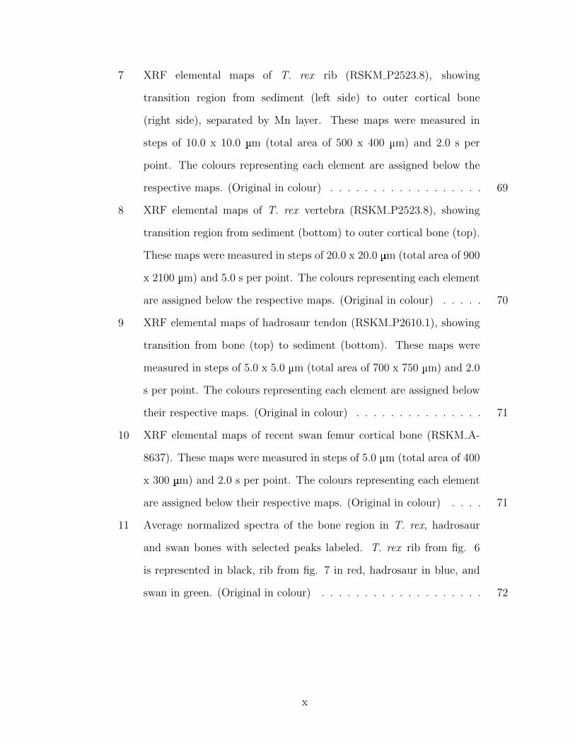
7 XRF elemental maps of T. rex rib (RSKM P2523.8), showing
transition region from sediment (left side) to outer cortical bone
(right side), separated by Mn layer. These maps were measured in
steps of 10.0 x 10.0 µm (total area of 500 x 400 µm) and 2.0 s per
point. The colours representing each element are assigned below the
respective maps. (Original in colour) . . . . . . . . . . . . . . . . . . 69
8 XRF elemental maps of T. rex vertebra (RSKM P2523.8), showing
transition region from sediment (bottom) to outer cortical bone (top).
These maps were measured in steps of 20.0 x 20.0 µm (total area of 900
x 2100 µm) and 5.0 s per point. The colours representing each element
are assigned below the respective maps. (Original in colour) . . . . . 70
9 XRF elemental maps of hadrosaur tendon (RSKM P2610.1), showing
transition from bone (top) to sediment (bottom). These maps were
measured in steps of 5.0 x 5.0 µm (total area of 700 x 750 µm) and 2.0
s per point. The colours representing each element are assigned below
their respective maps. (Original in colour) . . . . . . . . . . . . . . . 71
10 XRF elemental maps of recent swan femur cortical bone (RSKM A-
8637). These maps were measured in steps of 5.0 µm (total area of 400
x 300 µm) and 2.0 s per point. The colours representing each element
are assigned below their respective maps. (Original in colour) . . . . 71
11 Average normalized spectra of the bone region in T. rex, hadrosaur
and swan bones with selected peaks labeled. T. rex rib from fig. 6
is represented in black, rib from fig. 7 in red, hadrosaur in blue, and
swan in green. (Original in colour) . . . . . . . . . . . . . . . . . . . 72
x
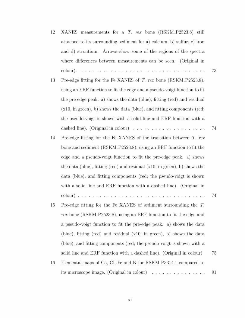
12 XANES measurements for a T. rex bone (RSKM P2523.8) still
attached to its surrounding sediment for a) calcium, b) sulfur, c) iron
and d) strontium. Arrows show some of the regions of the spectra
where differences between measurements can be seen. (Original in
colour). . . . . . . . . . . . . . . . . . . . . . . . . . . . . . . . . . . 73
13 Pre-edge fitting for the Fe XANES of T. rex bone (RSKM P2523.8),
using an ERF function to fit the edge and a pseudo-voigt function to fit
the pre-edge peak. a) shows the data (blue), fitting (red) and residual
(x10, in green), b) shows the data (blue), and fitting components (red;
the pseudo-voigt is shown with a solid line and ERF function with a
dashed line). (Original in colour) . . . . . . . . . . . . . . . . . . . . 74
14 Pre-edge fitting for the Fe XANES of the transition between T. rex
bone and sediment (RSKM P2523.8), using an ERF function to fit the
edge and a pseudo-voigt function to fit the pre-edge peak. a) shows
the data (blue), fitting (red) and residual (x10, in green), b) shows the
data (blue), and fitting components (red; the pseudo-voigt is shown
with a solid line and ERF function with a dashed line). (Original in
colour) . . . . . . . . . . . . . . . . . . . . . . . . . . . . . . . . . . . 74
15 Pre-edge fitting for the Fe XANES of sediment surrounding the T.
rex bone (RSKM P2523.8), using an ERF function to fit the edge and
a pseudo-voigt function to fit the pre-edge peak. a) shows the data
(blue), fitting (red) and residual (x10, in green), b) shows the data
(blue), and fitting components (red; the pseudo-voigt is shown with a
solid line and ERF function with a dashed line). (Original in colour) 75
16 Elemental maps of Ca, Cl, Fe and K for RSKM P3314.1 compared to
its microscope image. (Original in colour) . . . . . . . . . . . . . . . 91
xi

17 Elemental maps of Ca, Cl, Fe and K for RSKM P3314.2. (Original in
colour) . . . . . . . . . . . . . . . . . . . . . . . . . . . . . . . . . . . 91
18 Iron elemental distribution (top, split into two scans that correspond
to the head and thorax, and the abdomen) for Baltic amber ant RSKM
P3000.15 compared to its microscope image (bottom). Arrows show
examples of features that can be matched between elemental map and
microscope image. (Original in colour) . . . . . . . . . . . . . . . . . 93
19 Iron elemental distribution (left) for Baltic amber ant RSKM P3000.16
compared to its microscope image (right). White arrows show lines
with high amount of iron due to the infiltration of minerals in cracks
in the amber. (Original in colour) . . . . . . . . . . . . . . . . . . . . 93
20 Iron elemental distribution (left) for Baltic amber ant RSKM P3000.17
compared to its microscope image (right). (Original in colour) . . . . 94
21 Iron elemental map (left) for North Carolina amber SEMC NC
272-276 compared to its microscope image (right). In the elemental
map the scale goes from blue to red, representing lower to higher
concentrations of iron, respectively. White areas were not mapped.
(Original in colour) . . . . . . . . . . . . . . . . . . . . . . . . . . . 95
xii

22 a) CT rendering (ventral view) and b) XRF results for Baltic ant
P3000.15. The elemental maps show iron in red and calcium in green.
The overlay of the images can be seen in c). In a), the arrows show
the two surfaces visible in the image. The inner and outer surfaces
are represented by the blue and red arrows, respectively. In c), the
white arrow shows the regions where iron and calcium are present in
large quantity in the insect’s head. The orange arrows show areas
with higher iron concentrations in the insect’s abdomen. The blue
arrow shows the region with large quantity of calcium in the insect’s
abdomen. (Original in colour) . . . . . . . . . . . . . . . . . . . . . . 96
23 a) CT rendering (lateral view) and b) XRF results for Baltic ant
P3000.16. The elemental map shows iron in red and calcium in green.
The overlay of the images can be seen in c). (Original in colour) . . . 97
24 a) CT rendering (ventral view) and b) XRF results for Baltic ant
P3000.17. The elemental map shows iron in red and calcium in green.
The overlay of the images can be seen in c). (Original in colour) . . . 97
25 a) CT rendering of the head of Baltic amber ant RSKM P3000.15
(dorsal view) and b) the diagram of the preserved tissues observed in
the rendering. In b), the cuticle reinforcements of the tentorium are
represented in blue, mandibular muscles in pink, and traces of either
brain or digestive glands are in white. . . . . . . . . . . . . . . . . . . 98
xiii

26 Iron K-edge XANES results for measurements taken from the head
capsules of Baltic amber ants compared to a modern ant (RSKM
P3314.1). The spectra were normalized and are presented a) together
and b) stacked with 0.2 interval between different spectra. RSKM
P3000.15 is shown in blue, RSKM P3000.16 in purple, RSKM
P3000.17 in green, and RSKM P3314.1 in red. The arrows mark the
position of the edge. (Original in colour) . . . . . . . . . . . . . . . . 100
27 Iron pre-edge fit for Baltic ant specimen RSKM P3000.15, showing a)
fitting line and residual and b) a magnified image of the pre-edge region
and the individual functions used in the fitting. (Original in colour) . 100
28 Iron pre-edge fit for Baltic ant specimen RSKM P3000.16, showing a)
fitting line and residual and b) a magnified image of the pre-edge region
and the individual functions used in the fitting. (Original in colour) . 101
29 Iron pre-edge fit for Baltic ant specimen RSKM P3000.17, showing a)
fitting line and residual and b) a magnified image of the pre-edge region
and the individual functions used in the fitting. (Original in colour) . 101
30 Iron pre-edge fit for Baltic ant RSKM P3314.1, showing a) fitting line
and residual and b) a magnified image of the pre-edge region and the
individual functions used in the fitting. (Original in colour) . . . . . 102
31 Elemental maps for Ravenscrag Fm. turtle (RSKM P3314.1), which
includes part of the shell and of a rib bone. Orange arrows show
presence of strontium within marrow spaces in the shell. (Original in
colour) . . . . . . . . . . . . . . . . . . . . . . . . . . . . . . . . . . . 118
32 Elemental maps for Ravenscrag Fm. turtle (RSKM P3314.2), which
includes part of the shell and of a rib bone. (Original in colour) . . . 118
33 Elemental maps for Ravenscrag Fm. turtle (RSKM P3314.3), which
includes part of the shell and of a vertebra. (Original in colour) . . . 119
xiv
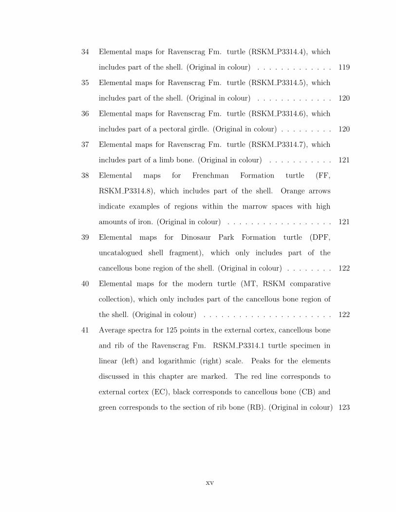
34 Elemental maps for Ravenscrag Fm. turtle (RSKM P3314.4), which
includes part of the shell. (Original in colour) . . . . . . . . . . . . . 119
35 Elemental maps for Ravenscrag Fm. turtle (RSKM P3314.5), which
includes part of the shell. (Original in colour) . . . . . . . . . . . . . 120
36 Elemental maps for Ravenscrag Fm. turtle (RSKM P3314.6), which
includes part of a pectoral girdle. (Original in colour) . . . . . . . . . 120
37 Elemental maps for Ravenscrag Fm. turtle (RSKM P3314.7), which
includes part of a limb bone. (Original in colour) . . . . . . . . . . . 121
38 Elemental maps for Frenchman Formation turtle (FF,
RSKM P3314.8), which includes part of the shell. Orange arrows
indicate examples of regions within the marrow spaces with high
amounts of iron. (Original in colour) . . . . . . . . . . . . . . . . . . 121
39 Elemental maps for Dinosaur Park Formation turtle (DPF,
uncatalogued shell fragment), which only includes part of the
cancellous bone region of the shell. (Original in colour) . . . . . . . . 122
40 Elemental maps for the modern turtle (MT, RSKM comparative
collection), which only includes part of the cancellous bone region of
the shell. (Original in colour) . . . . . . . . . . . . . . . . . . . . . . 122
41 Average spectra for 125 points in the external cortex, cancellous bone
and rib of the Ravenscrag Fm. RSKM P3314.1 turtle specimen in
linear (left) and logarithmic (right) scale. Peaks for the elements
discussed in this chapter are marked. The red line corresponds to
external cortex (EC), black corresponds to cancellous bone (CB) and
green corresponds to the section of rib bone (RB). (Original in colour) 123
xv

42 Average spectra for 125 points in the cancellous bone and vertebra
(Vert) of the Ravenscrag Fm. RSKM P3314.3 turtle specimen in linear
(left) and logarithmic (right) scale. Peaks for the elements discussed in
this chapter are marked. The black line corresponds to cancellous bone
(CB) and green corresponds to the section of vertebra bone (Vert).
(Original in colour) . . . . . . . . . . . . . . . . . . . . . . . . . . . . 124
43 Average spectra for 125 points in the external cortex, cancellous bone
and internal cortex of the Ravenscrag Fm. RSKM P3314.4 turtle
specimen in linear (left) and logarithmic (right) scale. Peaks for the
elements discussed in this chapter are marked. The red line
corresponds to external cortex (EC), black corresponds to cancellous
bone (CB) and blue corresponds to the internal cortex (IC). (Original
in colour) . . . . . . . . . . . . . . . . . . . . . . . . . . . . . . . . . 124
44 Average spectra for 125 points in the external cortex and cancellous
bone of the RSKM P3314.5 Ravenscrag Fm. turtle specimen in linear
(left) and logarithmic (right) scale. Peaks for the elements being
discussed in this chapter are marked. The red line corresponds to
external cortex (EC) and black corresponds to cancellous bone (CB).
(Original in colour) . . . . . . . . . . . . . . . . . . . . . . . . . . . . 125
45 Average spectra for 125 points in the external cortex and cancellous
bone of the FF turtle specimen (RSKM P3314.8) in linear (left) and
logarithmic (right) scale. Peaks for the elements being discussed in this
chapter are marked. The red line corresponds to external cortex (EC)
and black corresponds to cancellous bone (CB). (Original in colour) . 125
xvi

46 Average spectra for 125 points in the cancellous bone for a specimen
from each deposit and the modern turtle in linear (left) and
logarithmic (right) scale. Peaks for the elements being discussed in
this chapter are marked. The green line corresponds to the spectra of
the modern turtle (MT; RSKM comparative collection), cyan
corresponds to DPF (uncatalogued), orange corresponds to RF
(RSKM P3314.5), and purple corresponds to FF (RSKM P3314.8).
(Original in colour) . . . . . . . . . . . . . . . . . . . . . . . . . . . . 126
47 Average spectra for 125 points in the external cortex for a specimen
from Ravenscrag Formation (RSKM P3314.5) and the Frenchman
Formation (RSKM P3314.8) in linear (left) and logarithmic (right)
scale. Peaks for the elements being discussed in this chapter are
marked. The orange line corresponds to the spectra of
RSKM P3314.5 and purple corresponds to RSKM P3314.8. (Original
in colour) . . . . . . . . . . . . . . . . . . . . . . . . . . . . . . . . . 126
48 Elemental map for calcium and manganese for the Ravenscrag
Formation turtle RSKM P3314.5 with a) the same saturation for Mn
used in fig. 35 and b) the saturation changed so that the portion of
the distribution with lower intensity is shown in more detail.
(Original in colour) . . . . . . . . . . . . . . . . . . . . . . . . . . . . 128
49 Region (20 x 20 μm) of the skin sample associated with UALVP
53290 contaning a layer of approximately with substructures (left)
and the measured region (5 x 5 μm) containing one of these
substructures (inset and to right). The images were obtained in
transmission mode and, thus, dark areas correspond to detected
matter. The scale bar corresponds to 0.5 μm in the images. (Original
in colour) . . . . . . . . . . . . . . . . . . . . . . . . . . . . . . . . . 140
xvii
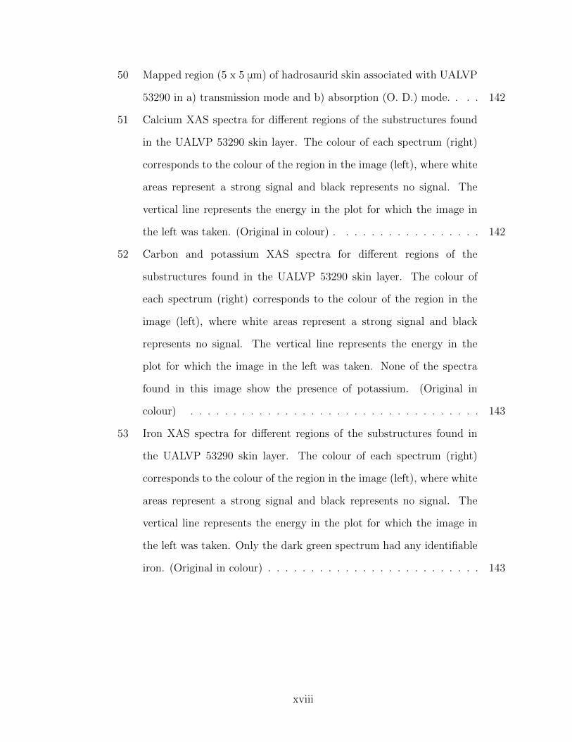
50 Mapped region (5 x 5 μm) of hadrosaurid skin associated with UALVP
53290 in a) transmission mode and b) absorption (O. D.) mode. . . . 142
51 Calcium XAS spectra for different regions of the substructures found
in the UALVP 53290 skin layer. The colour of each spectrum (right)
corresponds to the colour of the region in the image (left), where white
areas represent a strong signal and black represents no signal. The
vertical line represents the energy in the plot for which the image in
the left was taken. (Original in colour) . . . . . . . . . . . . . . . . . 142
52 Carbon and potassium XAS spectra for different regions of the
substructures found in the UALVP 53290 skin layer. The colour of
each spectrum (right) corresponds to the colour of the region in the
image (left), where white areas represent a strong signal and black
represents no signal. The vertical line represents the energy in the
plot for which the image in the left was taken. None of the spectra
found in this image show the presence of potassium. (Original in
colour) . . . . . . . . . . . . . . . . . . . . . . . . . . . . . . . . . . 143
53 Iron XAS spectra for different regions of the substructures found in
the UALVP 53290 skin layer. The colour of each spectrum (right)
corresponds to the colour of the region in the image (left), where white
areas represent a strong signal and black represents no signal. The
vertical line represents the energy in the plot for which the image in
the left was taken. Only the dark green spectrum had any identifiable
iron. (Original in colour) . . . . . . . . . . . . . . . . . . . . . . . . . 143
xviii
54 Manganese XAS spectra for different regions of the substructures found
in the UALVP 53290 skin layer. The colour of each spectrum (right)
corresponds to the colour of the region in the image (left), where white
areas represent a strong signal and black represents no signal. The
vertical line represents the energy in the plot for which the image in
the left was taken. Manganese was not found in any region of the
measured area. (Original in colour) . . . . . . . . . . . . . . . . . . . 144
55 Map showing the distribution of the two different states of calcium in
fossil skin associated with UALVP 53290, where a) shows the
distribution of the spectrum found in red in fig. 51 (calcium 1), b)
shows the distribution of the other spectrum (calcium 2) and c)
shows a combination of both distributions. The circle in a) shows the
approximated region where the substructure is believed to be. The
arrow shows the region of strong calcium 1. (Original in colour) . . . 145
56 Average spectra of calcium 1 (blue) and calcium 2 (red) in fossil skin
associated with UALVP 53290, calculated based on the regions where
the spectra are found. Blue arrows point at the main peaks of the
spectra, while black arrows point at the secondary peaks. The red
arrow points at detail at the second main peak, where two “bumps”
can be observed. (Original in colour) . . . . . . . . . . . . . . . . . . 145
57 Map showing the distribution of the three different states of carbon
in fossil skin associated with UALVP 53290, where a) shows the
distribution of carbon-1, b) shows the distribution of carbon-2, c)
shows the distribution of carbon-3 and d) shows a combination of all
distributions. (Original in colour) . . . . . . . . . . . . . . . . . . . . 147
xix
58 Average spectra of carbon 1, 2 and 3 in fossil skin associated with
UALVP 53290, calculated based on the regions where the spectra are
found. (Original in colour) . . . . . . . . . . . . . . . . . . . . . . . . 147
59 Map showing the distribution of the only measured state of iron in fossil
skin associated with UALVP 53290 as seen in the green spectrum of
fig. 53. (Original in colour) . . . . . . . . . . . . . . . . . . . . . . . 148
60 Average spectrum of iron in fossil skin associated with UALVP
53290, calculated based on the regions where the spectrum are found.
(Original in colour) . . . . . . . . . . . . . . . . . . . . . . . . . . . . 149
61 Maps comparing the distributions of carbon-1, iron and a) calcium-1
and b) calcium-2 in fossil skin associated with UALVP 53290. (Original
in colour) . . . . . . . . . . . . . . . . . . . . . . . . . . . . . . . . . 149
62 Maps comparing the distributions of carbon-2, iron and a) calcium-1
and b) calcium-2 in fossil skin associated with UALVP 53290. (Original
in colour) . . . . . . . . . . . . . . . . . . . . . . . . . . . . . . . . . 150
63 Distribution of the ratio iron/calcium for a) T. rex rib
RSKM P2523.8 (fig. 6), b) T. rex rib RSKM P2523.8 (fig. 7), c)
DPP turtle (uncatalogued) and d) RF turtle RSKM P3314.5. The
numbers on the axes correspond to the number of steps in each
direction. (Original in colour) . . . . . . . . . . . . . . . . . . . . . . 157
64 Distribution of the ratio manganese/calcium for a) T. rex rib
RSKM P2523.8 (fig. 6), b) T. rex rib RSKM P2523.8 (fig. 7), c)
DPP turtle (uncatalogued) and d) RF turtle RSKM P3314.5. The
numbers on the axes correspond to the number of steps in each
direction. (Original in colour) . . . . . . . . . . . . . . . . . . . . . . 158
xx

65 Distribution of the ratio strontium/calcium for a) T. rex rib
RSKM P2523.8 (fig. 6), b) T. rex rib RSKM P2523.8 (fig. 7), c)
DPP turtle (uncatalogued) and d) RF turtle RSKM P3314.5. The
numbers on the axes correspond to the number of steps in each
direction. (Original in colour) . . . . . . . . . . . . . . . . . . . . . . 159
66 Distribution of the ratio yttrium/calcium for a) T. rex rib
RSKM P2523.8 (fig. 6), b) T. rex rib RSKM P2523.8 (fig. 7), c)
DPP turtle (uncatalogued) and d) RF turtle RSKM P3314.5. The
numbers on the axes correspond to the number of steps in each
direction. (Original in colour) . . . . . . . . . . . . . . . . . . . . . . 160
67 Scatter plots relating calcium and iron for dinosaur bones. The
quantities are represented in arbitrary units, corresponding to the
number of counts under the peak associated to a given element,
corrected for variations in the electron beam current which affects the
X-ray beam intensity at the synchrotron facility. . . . . . . . . . . . 161
68 Scatter plots relating calcium and iron for turtle bones. The
quantities are represented in arbitrary units, corresponding to the
number of counts under the peak associated to a given element,
corrected for variations in the electron beam current which affects the
X-ray beam intensity at the synchrotron facility. . . . . . . . . . . . . 161
69 Scatter plots relating calcium and manganese for dinosaur bones.
The quantities are represented in arbitrary units, corresponding to
the number of counts under the peak associated to a given element,
corrected for variations in the electron beam current which affects the
X-ray beam intensity at the synchrotron facility. . . . . . . . . . . . 162
xxi

70 Scatter plots relating calcium and iron for dinosaur bones. The
quantities are represented in arbitrary units, corresponding to the
number of counts under the peak associated to a given element,
corrected for variations in the electron beam current which affects the
X-ray beam intensity at the synchrotron facility. . . . . . . . . . . . 162
71 Schematics of the magnetic field in a quadrupole magnet. . . . . . . 206
72 Simplified representation of the electron oscillations within a wiggler,
as well as the radiation produced by their acceleration. (Original in
colour) . . . . . . . . . . . . . . . . . . . . . . . . . . . . . . . . . . . 214
73 Schematic representation of incident light on a finite slab of material
and some of its possible reflections [113]. . . . . . . . . . . . . . . . . 226
xxii
List of Abbreviations
BMIT Bio-Medical Imaging and Therapy Facility
CB cancellous bone
CC Creative Commons
CLS Canadian Light Source
CLSM Confocal Laser Scanning Microscopy
CT Computed Tomography
DPF Dinosaur Park Formation
EC external cortex
EDS Energy Dispersive Spectrometer
EDX Energy Dispersive X-ray Spectroscopy
ERF error function
ESRF European Synchrotron Research Facility
eV electronvolt
EXAFS Extended X-ray Absoprtion Fine Structure
FEG-SEM Field Emission Gun Scanning Electron Microscopy
FF Frenchman Formation
FMS Full Multiple Scattering
FTIR Fourier-Transform Infrared Spectroscopy
IC internal cortex
IR Infrared
K Cretaceous
KB Kirkpatrick-Baez
MT modern turtle
NDF number of degrees of freedom
NEXAFS Near Edge X-ray Absorption Fine Structure
OD optical density
xxiii
Pg Paleogene
rf radio frequency
RGB red-green-blue
RF Ravenscrag Formation
ROI region of interest
RSM Royal Saskatchewan Museum
SEM Scanning Electron Microscopy
SM Soft X-ray Spectromicroscopy Beamline
SRS-XRF Synchrotron Rapid Scanning X-ray Fluorescence
STXM Scanning Transmission X-ray Microscopy
SXRMB Soft X-ray Microcharacterization Beamline
TEM Transmission Electron Microscopy
ToF-SIMS Time-of-Flight Secondary Ion Mass Spectroscopy
VERSPERS Very Sensitive Elemental and Structural Probe Employing Radiation
from a Synchrotron
XAFS X-ray Absorption Fine Structure
XANES X-ray Absorption Near Edge Structure
XAS X-ray Absoprtion Spectroscospy
XPS X-ray Photoelectron Spectroscopy
XRF X-ray Fluorescence
xxiv
1 Introduction and thesis structure
For many years, fossils were seen as lithified remains that mostly preserved the
shape of the original animal, and, in some cases, materials that were originally
mineralized, such as bones and teeth. That conception has changed in the past
decades due to several published results suggesting the presence of preserved
molecules and structures in fossils (e.g., [1, 2, 3, 4, 5]). These findings changed the
research goals and the types of analyses being performed in fossils. But, with the
changes in the type of studies developed in the field of palaeontology, the techniques
used for the analysis of specimens also have to change. Such changes include the
opportunity for multidisciplinary research with the application of techniques from
other disciplines to study preservation and taphonomic alterations in fossils.
Taphonomy is the study of the processes that remains undergo between the
animal’s death and discovery [6]. This includes physical effects, such as transport
and weathering, and chemical effects that alter how the remains are positioned,
where they are located, the way they look, and their composition [6]. The quality of
the preservation in fossils is determined by how the remains are affected by these
processes and when in their taphonomic history they occur. As an example, the
fossilization of soft tissues depends on the early mineralization of the remains, such
that they are preserved before significant decay occurs [6, 7].
The main goal of this thesis is to use synchrotron-based techniques (X-ray
fluorescence and X-ray absorption fine structure, in particular) to study the
taphonomy of different fossil specimens, including dinosaur bones and skin, turtle
bones and insect inclusions in amber. The objective is to study the extent to which
these techniques can be applied to different specimens to obtain information on
their preservation and taphonomic alterations. With the use of synchrotron
techniques, I want to be able to identify some of the possible mechanisms
responsible for the exceptional preservation of fossils (especially soft tissues), and to
1

understand some of the diagenetic changes the specimens undergo. This thesis is
primarily an application of high-energy physics to palaeontological samples. It
extends a new suite of techniques to a wide range of palaeontological samples to test
the limits of these techniques.
This thesis is divided into nine chapters, including this introduction. Chapters 2
and 3 provide the theoretical background for the discussions presented in the later
chapters. Chapter 2 introduces the main concept of taphonomy in general, and the
special conditions required to preserve vertebrates and invertebrates (specifically
those preserved in amber). It also includes the explanation of the main physical and
chemical alterations experienced by fossils. Chapter 3 discusses synchrotron light,
how it is produced, its properties, and the main techniques used in the analyses for
this thesis, X-ray fluorescence (XRF) and X-ray absorption fine structure (XAFS).
Chapters 4, 5, 6 and 7 each discuss the research developed based upon different sets
of specimens. The chapter structure contains a brief introduction and the theory
specific to the research being developed (if the topic has not been covered in chapter
2 or 3), as well as the methods employed, the results, discussions, and conclusions
relative to that particular topic. This is followed by chapter 8, which presents a
discussion combining data from the previous four chapters, and chapter 9 with the
conclusions for the thesis.
Chapter 4 presents results from the research developed on the Tyrannosaurus rex
(T. rex ) informally known as “Scotty”. In this study, I compared chemical maps of
the T. rex bones with those from a hadrosaur found in the same formation, and
from an extant swan, in order to identify diagenetic alterations and the specific
characteristics responsible for “Scotty’s” preservation. In chapter 5, I discuss the
application of synchrotron techniques to non-destructively characterize the chemical
composition of insect inclusions in amber. The goals of this research were to
understand the strengths and pitfalls of using XRF to chemically map inclusions
2

non-destructively, and to apply this technique to study ants in Baltic amber and
their preservation. Chapter 6 discusses the research I developed on turtle shells with
the intention of understanding how different bone tissue types, age, and depositional
environment are affected by taphonomic modifications. The research I developed to
characterize a very rare specimen of hadrosaur skin is discussed in chapter 7 (as
part of a larger effort involving other researchers) to characterize a rare specimen of
hadrosaur skin. Previous results have shown that the specimen preserved skin-like
(i.e., epidermal) layers composed of approximately round substructures. My
objective was to chemically characterize one of these single substructures in order to
find possible mechanisms responsible for the preservation of this specimen. Chapter
8 synthesizes some of the data from chapters 4 and 6. It also compares the results of
measurements in terms of the relative concentration between certain chemical
elements, and how they correlate to one another.
All the measurements, analyses and discussions described in this thesis were
developed by me, unless it is stated otherwise.
3
2 Taphonomy
2.1 Abstract
Taphonomy is the name given to the study of the processes remains go through
from death until their discovery. Taphonomic studies have been developed by
researchers for centuries. They are essencial for the understanding of how fossils are
changed and preserved, and how they relate to each other and their
palaeoenvironment. Taphonomic effects can be divided into physical and chemical
processes. Each of these processes will produce distinct types of modifications
within the fossil remains. The objective of this review is to provide an overall
introduction to the taphonomic process in general, and the details of these processes
in the context of vertebrate and insect remains. I will also comment on the
conditions that result on exceptional preservation scenarios, also known as
Lagerstatten. This review will be used as the background for all discussions in
subsequent chapters of this thesis. They will include studies on the taphonomic
alterations encountered by different specimens of dinosaurs, turtles, and insects (as
amber inclusions), some of which are exceptionally preserved.
2.2 Introduction
The term taphonomy was first proposed by Efremov in 1940 [8] as the science that uses
concepts from both geology and biology to study the history of specimens, from death
to diagenesis. This, however, was not the first time that taphonomy was studied.
In fact, taphonomic researches had been developed since Leonardo da Vinci in the
15th century, who used the observation of the remains of bivalves and their extant
counterparts to conclude that the remains found in Monferrato (Italy) mountains had
not been transported by the biblical deluge, but were originally from that location
[6].
4

By the end of the 19th and beginning of the 20th century, the study of
taphonomy was mostly centered around paleoenvironmental arguments. Efremov, in
particular, was a vertebrate paleontologist who focused on the loss of information
due to taphonomic processes, which associated the science of taphonomy with the
study of biases in the fossil record produced by these processes [6, 8]. Behrensmeyer
and Kidwell [9] were critics of this limited interpretation of taphonomy, as fossil
assemblages can also be changed over time due to the addition and alteration of
information. They saw the addition of certain chemical elements that were not
originally present in the remains, or changes in the location where the remains are
found as more than just a loss of information. Thus, they proposed a new definition
for this science: “the study of processes of preservation and how they affect
information in the fossil record”. In the most recent applications, taphonomy sets
methods to study palaeobiology [10]. These allow for better answers for questions
regarding trends in biodiversity, characteristics of major extinctions, and rates of
evolution, among others [10].
The modern study of taphonomy can be divided into two branches; 1)
biostratinomy, including events that occur following the death of the animal, and
extending until its burial, and 2) diagenesis, encompassing events that occur after
burial, extending until the remains are found [6]. Since some of the processes in
these two stages are continuous and the limits between the two are somewhat
blurred, the following discussion will treat them together.
2.3 Taphonomy of vertebrates
2.3.1 Decay
According to Weigelt [11], when an animal dies, the lower temperature of the body
causes the muscles to contract, limiting joint mobility. This process is called rigor
mortis and it sets, usually, around ten hours after death and lasts between ten and
5
eighteen hours. Once rigor mortis is over, the decay and putrefaction processes begin.
The decomposition of the remains is caused both by aerobic (external to the body) and
anaerobic (internal to the body) bacteria, with contributions from other organisms,
such as insects, which will lay their eggs in carcasses.
Weigelt [11] also proposed a very well-defined sequence for the disarticulation of
mammals. His observations suggested which parts of the body are more likely to
disarticulate first, such as the lower jaws (due to the way they are attached to the
body and the preference of predators and scavengers for attacking animals around
the head and neck). This hypothesis was challenged by Toots [12], who concluded
that, although rules can be established for the normal sequence of disarticulation of
carcasses, they depend on the taxonomic group being observed. For Toots, the
sequence of disarticulation depends on the type of joint and the interlocking
mechanisms keeping it together, and the amount of easily decomposable material
around the articulation. Therefore, aside from the activity of scavengers, bones that
are connected very strongly, such as the animal’s vertebral column, will be the last
to decay and disassociate. Meanwhile, body regions surrounded by a large amount
of easily decomposable material, such as the abdomen, will decompose very fast.
This is also true for tissues holding joints in vertebrates. The work of Hill and
Behrensmeyer [13], however, studying the disarticulation of African mammals,
showed that the process is very consistent among animals of different taxa. Hill and
Behrensmeyer [13] believe the differences observed by Toots [12] could be specific to
the animals he was studying, and that Weigelt’s [11] hypothesis was probably more
correct.
2.3.2 Physical processes
Weathering Weathering refers to the effects on remains caused by exposure to
environmental factors. The weathering of mammal bones subject to the natural
6

environment has been studied by Behrensmeyer [14] based on the observation of bones
in Amboseli Park, Kenya. She observed that the exposed side of bones exhibited more
weathering effects than the side touching the soil. These differences can be attributed
to variations in environmental temperature, and moisture (the bone parts in contact
with the soil would be less affected by these conditions). This idea was further
supported by the fact that buried bones, which are not affected by the variations
in the soil surface, did not show significant weathering. Moreover, parts of bones
extending more than 10 cm above the soil showed less weathering than lower bones.
In special cases, weathering may act differently. For example, when the soil is
alkaline and salt crystals form on the surface of bones, the part of a bone in contact
with the soil weathers faster than that of the exposed side [14]. The action of insects,
roots and bacteria can also cause different patterns of weathering [14, 10]. Weathering
can also be caused by physical oxidation, hydrolysis, UV light, and dissolution, among
other factors [10].
Behrensmeyer [14] suggested six weathering stages to be used in comparisons
between fossils and modern remains, and the corresponding exposure time that would
result in these stages, based on carcasses observations:
Stage 0: Bones do not present cracking or flaking caused by weathering. They
can also present other preserved structures, such as skin, muscle, ligaments or
marrow tissue. This corresponds to 0–1 years exposed.
Stage 1: Bones present cracks, usually, in the direction of the fiber structure.
Cracking can also be present in the articulation surface of bones. Sometimes,
other tissues are also present. This corresponds to 0–3 years exposed.
Stage 2: Initially, flaking occurs in the outermost bone layers, usually associated
with cracks. Eventually, the inner layers of the bone also show flaking until the
outer layers of bone are completely gone. Portions of ligament, cartilage and
7

skin tissues can also be present. This corresponds to 2–6 years exposed.
Stage 3: Patches to whole bones are uniformly covered by a rough and
homogeneously weathered layer of compact bone, which does not penetrate
more than 1.0–1.5 mm deep. Other tissue presevation at this stage is rare.
This corresponds to 4–15+ years exposed.
Stage 4: Overall, the bones present a rough and fibrous surface. Weathering can
penetrate to the bone’s inner cortical or medullary layers; splinters are formed
and can separate from the bone if it is moved. This corresponds to 6–15+ years
exposed.
Stage 5: Bones are falling apart with splinters around them. The bones’ original
shape can be difficult to determine and they become very fragile and easily
breakable. This corresponds to 6–15+ years exposed.
In case of heterogeneity, the patch with the most advanced stage is to be considered,
and, when possible, edges and damaged surfaces of bones should not be used in this
analysis.
These stages have been used with success over the years to characterize remains.
However, identifying weathering patterns from other features acquired after burial or
during diagenesis can sometimes be complicated [10].
Transport Transport is the effect of moving remains from one location to
another. The degree of transport will determine if fossils are autochtonous (found in
the same area where the animals died), parautochtonous (moved but not
transported to a different community1, which usually includes disarticulation or
reorientation), or allochthonous (found far from where the animal died, sometimes
1Community here refers to the set of populations sharing the same geographical area at the sametime.
8
mixed with other assemblages) [6, 15]. Both fresh remains and fossilized bones can
be transported, the latter is usually referred to as reworking.
Apart from predation and scavenging, a common transport means for animal
remains and sediments is water. The motion of the fluid may cause the transport
or reorientation of bones and the transport of sediments related to their burial. The
capacity of transport by a fluid depends on its properties of viscosity and density [6].
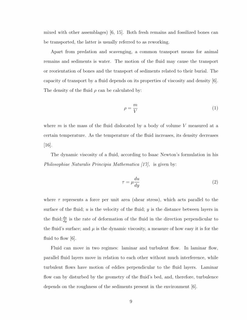
The density of the fluid ρ can be calculated by:
ρ =m
V(1)
where m is the mass of the fluid dislocated by a body of volume V measured at a
certain temperature. As the temperature of the fluid increases, its density decreases
[16].
The dynamic viscosity of a fluid, according to Isaac Newton’s formulation in his
Philosophiae Naturalis Principia Mathematica [17], is given by:
τ = µdu
dy(2)
where τ represents a force per unit area (shear stress), which acts parallel to the
surface of the fluid; u is the velocity of the fluid; y is the distance between layers in
the fluid;dudy
is the rate of deformation of the fluid in the direction perpendicular to
the fluid’s surface; and µ is the dynamic viscosity, a measure of how easy it is for the
fluid to flow [6].
Fluid can move in two regimes: laminar and turbulent flow. In laminar flow,
parallel fluid layers move in relation to each other without much interference, while
turbulent flows have motion of eddies perpendicular to the fluid layers. Laminar
flow can by disturbed by the geometry of the fluid’s bed, and, therefore, turbulence
depends on the roughness of the sediments present in the environment [6].
9

According to Reynolds [18], eddies are produced when the quantity, known as
Reynolds number, is above a certain threshold:
Re =cρU
µ(3)
where c is a linear parameter, such as the radius of a tube in which the fluid is moving;
ρ is the density of the fluid; U is the mean velocity of the fluid and µ is the dynamic
viscosity of the fluid.
A body will be moved by a fluid if the force acting on it is larger than the force
holding the body in place (usually friction). The former depends on the fluid velocity,
shear stress, fluid viscosity and body size, shape and density [6].
Many experiments have been performed to determine the behaviour of bones and
other remains when they are subjected to water currents. In his pioneering work,
Voorhies [19] used a 45-feet-long by 4-feet-wide stream table with a sand bed (particle
size between 0.25 and 0.50 mm) in which the velocity of the water could be controlled
to study how mammal bones behave under different conditions. The results showed
that long bones, such as the femur or tibia, tend to align parallel or perpendicular
to the current. The latter orientation was more common when the water levels were
shallow and part of the bone was exposed. The parallel alignment was more common
when the bone was completely submerged. They also tend to have their larger ends
oriented downstream.
Voorhies [19] also tested other types of bones with complex shapes, such as jaws,
which tend to align convex-up when higher fluid velocities are reached. Small bones
were more affected by the roughness of the bed than larger bones, and, in some
occasions, became trapped and were buried as the materials moved. Although the
velocities achieved in this experiment were not enough to move most heavier skulls,
when they moved, their long axes remained perpendicular to the current while they
10

rolled. The pelvis tended to align upside-down, with the ilia oriented downstream.
He did not notice patterns when looking at ribs and vertebrae.
In a second series of experiments, Voorhies [19] used the same setup on
disarticulated remains of coyote and sheep in order to evaluate the sequence in
which they are transported. He noted three groups of bones: in the first, the bones
moved immediately when subjected to a current, by saltation or flotation (e.g., ribs,
vertebrae); in the second, the bones tended to move some time after the bones in
group one, by traction (e.g., femur, tibia, pelvis); in the third, the bones tend to
resist the current and to stay in their original positions within the velocities tested
(e.g., skull, mandible). These groups are now referred to as “Voorhies’ groups”.
Later research by Behrensmeyer [20] and Hanson [21] showed that most transport
of bones in groups two and three occurs during floods, when the body of water moves
faster and has the force necessary to move these bones. More recently, Coard [22]
experimentally determined that articulated remains have a higher transport potential
than their disarticulated counterparts and the same can be said, to a lesser extent,
about dry bones in comparison to wet ones.
Dodson [23] was one of the first researchers to extend this type of analysis to fossil
reptile bones. When studying the Oldman Formation (Alberta, Canada), he placed
bones in eleven classes, according to how complete and articulated the remains were
when found. The specimens varied from complete and articulated skeletons, some
with fossilized integument, to isolated bones, reflecting different conditions of burial
and transport.
Experimental studies of the behaviour of dinosaur bones in fluvial environments
have been conducted by Peterson and Bigalke [24], using casts of pachycephalosaurid
domes with mass and density similar to non fossilized bones. Their research suggested
that, although the mammal models discussed before provide good approximations to
the behaviour of their specimens, the shape and size of the dome result in differences
11

in transport distances and orientations. Ultimately, their study indicated that more
research is necessary to better understand the transport of dinosaur remains and their
peculiarities.
Time-Averaging The time scales involved in biology (e.g., organisms’ lifespans)
are very short when compared to the geological timescale. Therefore, before large
geological changes take place, many organisms will usually live and die in a region.
The result is that many animals may die and have their remains accumulated over the
span of years before they are buried by sediments. The fossils later found will thus be
an average of the life in that space over many years (up to hundreds of thousands of
years, depending on the depositional environment). This is known as time-averaging
and must be considered when interpreting a fossil assemblage [6, 25]. Time-averaging
would not occur if, for example, a large catastrophic event occurred, immediately
burying the animals.
The effects of time-averaging in fossil assemblages are discussed in [6], and for
terrestrial settings more specifically in works such as [25]. One of these effects is
related to the abundance of fossils of a single species. For a long accumulation of
fossils in an area, more members from a single species will die in the region. This
means that species that are preserved easily, or that live in the same region for long
time intervals will have a disproportionate number of preserved individuals, even if
they were not dominant at the time of their deaths.
Time-averaging can also interfere in the estimated diversity of a paleoenvironment.
Depending on the duration of the averaging process, many communities can have
their members included in an assemblage, and these could be difficult to differentiate
from a community with a larger diversity living for a longer amount of time in the
region. Time-averaging also smooths out short-term variations in the local diversity,
causing problems in the interpretation of the local paleoecology, since species that
12

never coexisted would seem like they did [15].
Stratigraphic disorder can also be caused by time-averaging, where the
chronological order of the deposition of remains in relation to the stratigraphic
layers is not maintained due to reworking, or due to condensing of fossil horizons
through winnowing of sediments [15].
Bioturbation Bioturbation refers to the movement of sediments caused by the
action of living organisms, which can alter the chemistry and preservation of
remains. It will also modify the stratigraphic record by eliminating the short-term,
high-frequency events (e.g., occasional floods) while maintaining the long-term,
lower-frequency ones (e.g., formation of a lake in the region) [6]. While terrestrial
bioturbation has not been studied in depth (most research focuses on feeding traces
and trackways), many models have been developed to explain bioturbation in
aquatic systems. The diffusion models for bioturbation are the most famous, and
they are based on chemical and thermal mathematical diffusion models [6, 26].
As an example, a prominent diffusion model for deep-sea water was proposed by
Guinasso and Schink [27]. In this model, the concentration distribution of a tracer
material is studied both in terms of depth and time, according to the differential
equation:
∂c
∂t= D
∂2c
∂x2− v ∂c
∂x(4)
where c is the concentration (measured in cm−3), t is the time (measured in kiloyears),
D is the eddy diffusion coefficient (measured in cm2 kyr−1), v is the sedimentation
rate (measured in cm kyr−1) and x is the depth from the surface (measured in cm).
This model successfully describes the ranges known for some systems even though it
has simplifications (such as the fact that D, in this model, does not vary with depth).
The diffusion models have been successful in modeling in these conditions;
13

however, the assumption that thermochemical diffusion and bioturbation work in
the same way is not necessarily correct [6]. Diffusion models should only be applied
in cases in which the particles in the sediment move randomly across space and
time. The distance travelled by the particles are much smaller, on average, than the
scale of the process being considered, and the time considered for mixing events is
much smaller than the time necessary for reaction or for the introduction of the
tracer in the sediments [6].
2.3.3 Chemical processes
Apart from the physical processes discussed in section 2.3.2, animal remains also go
through chemical alterations over time. Some processes occur fairly early in the
diagenetic history of the fossil, but the interactions between animal tissue and
sediment persist over the years. Mineralization in fossils can produce detailed
structural preservation by 1) permineralization, when fluids with minerals infiltrate
the remains in sediments rich in organic matter, creating molds of the structures; 2)
petrification, when minerals are added to hardparts, usually when they are porous
enough to facilitate the process; 3) replacement, when minerals substitute other
materials [6, 28]. How quickly tissue mineralization occurs in relation to its decay is
a factor in its preservation. Early mineralization plays an important part in the
preservation of fossils [6, 29]. Therefore, this section will discuss the alterations
caused by chemical processes throughout the remains’ history, followed, in section
2.4, by a discussion on how different vertebrate structures are preserved in this
context, and the conditions necessary for preservation to occur.
Silicification Silicification is the process of permineralization, petrification or
replacement by silicon-based minerals, such as quartz and opal. These minerals can
form crystals of various sizes, influencing which features are preserved in this
14

process [6]. The source of silicon is found in saturated or near-saturated solutions,
in the form of silic acid (H4SiO4). This acid can eliminate water to form silica
(SiO2) and is usually deposited in animal remains via water with neutral or slightly
acidic pH. Several mechanisms can give origin to the diluted silicon, such as volcanic
and hydrothermal activities or biogenic activity [6, 30]. Some studies (e.g., [30, 31])
suggested that biogenic silicon might enhance, or even control the chances for
silicification to occur, introducing an important bias in the fossil record. According
to [30], organisms living in close proximity to siliceous sponges had a higher chance
of preservation through silicification. The number of silicified fossils in marine
environments may dramatically fall in geological periods when these sponges were
not as common [30].
In terrestrial settings, this method of preservation is more common for wood and
invertebrates. However, examples have been found of vertebrate preservation through
silicification. One of such discovery was reported by Channing et al [32], where a bird
from a Quaternary hot spring was found silicified with a remarkable preservation of
details, which was probably facilitated by the action of microbial organisms. Another
example is the Australian Cretaceous Griman Creek Formation, where terrestrial
faunas and floras were preserved in opal [33]. Among the animals found are dinosaurs
[34], molluscs [35], and mammals [36].
Pyritization Pyritization is the mineralization process by pyrite. In general,
pyritization occurs when sulfides (usually produced by the reduction of sulfates)
interact with dissolved iron. The iron is usually produced by one of the three
following processes:
H2S + 2FeOOH + 4H+ → S0 + 2Fe2+ + 4H2O (5)
CH2O + 4FeOOH + 8H+ → CO2 + 4Fe2+ + 7H2O (6)
15

7O2 + 2FeS2 + 2H2O → 2Fe2+ + 4SO2−4 + 4H+ (7)
These processes represent the reduction of iron oxides by sulfide, the reduction of
iron oxides by organic compounds, and the oxidation of iron sulfides, respectively
[6, 29, 28]. The resulting iron sulfides can take different shapes, but, framboidal
pyrite, for example, is obtained as follows:
18CH2O + 9SO2−4 → 18HCO−3 + 9H2S (8)
6FeOOH + 9H2S → 6FeS + 3S0 + 12HsO (9)
3FeS + S0 → Fe3S4 (10)
Fe3S4 + 2S0 → 3FeS2 (11)
These equations show the formation of pyrite as a process, where pyrite is just the
end product of the reaction [6, 28]. Also, since six FeS are formed in equation 9,
and only three can be converted into pyrite with elemental sulfur produced in this
reaction (see equations 10 and 11), another source of sulfur is necessary so that all
the FeS can be converted into pyrite. This source is still unknown [6, 28].
In practice, porewaters cannot contain a large concentration of both dissolved
sulfide and iron: when the concentration of one increases, the other decreases rapidly.
As a result, the mechanism that allows pyritization of fossil vertebrates is the decay
of organic matter [37]. In this case, the decay of the organics produce sulfur locally,
which can be combined with iron present in the water for pyrite formation. The
preservation of soft-tissue through pyritization will occur when decaying carcasses
are placed in organic-poor sediments and the concentration of dissolved Fe is much
higher than the concentration of sulfides being produced by decay [29]. That could
occur for example with the presence of another factor (such as low organic carbon
content) that limits sulfate reduction [29]. These sulfides can also be produced by
16

bacterial sulfate reduction when microbial mats are present in the specimen [38].
Phosphatization Phosphatization occurs when a large concentration of
phosphorus is available. This element usually belongs to the apatite group (i.e.,
with general formula Ca10(PO4, CO3)6(F,OH,Cl)≥2, where PO3−4 and CO2−
3 can
substitute one another) [6]. According to Briggs [29], the decay of organic matter
and the dissolution of bioapatite, the fixation in microbial mats, and adsorption of
Fe(II) ions produced by Fe(III) reduction are three agents that are the most
important when increasing the concentration of phosphorus in the environment.
Although the conditions allowing for the preservation of soft parts are localized,
when it occurs, the highest levels of preservation are possible in phosphatization,
including the preservation of cellular details [6].
Dissolved phosphorus usually combines with iron, but when in an anoxic
environment, the iron is reduced and the phosphate concentration increases.
Therefore, phosphatization occurs when the carcass remains at the oxic/anoxic
interface long enough for phosphorus to be liberated after the reduction of iron [39].
However, in some cases, the conditions local to a specimen can result in preferential
phosphatization of a single species. A good example of this phenomenon is when the
animal itself provides enough phosphorus and microbial activity responsible for its
decay provides the reducing environment [40]. In this case, the microbial activity
will determine the level of preservation: if the decay has been generally extensive,
most original features will be replaced by phosphatising microbes; while, if only
some parts of the animal have decayed, other parts can be preserved in great detail.
The precipitation of calcium carbonate or calcium phosphate (from apatite) is
controlled by local conditions (mainly the pH of pore waters) and can vary within
the same individual. Consequently, different parts of the animal can contain either
carbonates or phosphates [29]. The presence of microbial mats may contribute to
17

trapping phosphate and creating the reduced pH environment, which can promote
phosphatization.
2.4 Preservation in vertebrates
The physical and chemical taphonomic agents previously mentioned act differently
depending on the tissue being analyzed. In the next section, the most important of
these agents and how they affect each of the commonly preserved vertebrate tissues
will be discussed, with special attention to dinosaur remains.
2.4.1 Bones
Bones are mostly made of hydroxyapatite, water and organic compounds, of which
the most common is collagen. Skeletal remains can experience a series of processes
that will lead to their destruction or preservation during fossilization and diagenesis
[41]. Before burial, the most common source of damage to bones is predation or
scavenging. They can leave marks on the bones, such as scratches, punctures, and
fractures. Chemical alterations can also be caused by digestion, which can create
changes in the Ca/P ratios, or the concentration of elements such as Sr, Mn, Fe and
Zn, among others [42]. Additional pre-burial processes include weathering, which can
cause bone fragmentation, an increase in strontium levels, crystallographic alterations,
and protein degradation. Trampling, which can also cause bone fragmentation; and
transport, which can lead to the abrasion, dispersal, or artificial accumulation of
bones can also occur [43].
After burial, the bones may be subject to bioturbation, damages caused by plant
roots and lichens, or dissolution and corrosion of bone material by the surrounding
soil. The bones can also go through diagenetic chemical changes, which can cause an
increase in the amounts of Ca, Mg, S, Fe, Sr [41] and Y [44]. The types and degrees
of changes experienced are correlated more strongly with the nature of the sediments
18
around the bone than to the duration of the diagenetic process [41].
Apart from the mineral portion of the bones, many recent studies have focused
on the preservation of collagen, a protein that gives bones elasticity and resistance
to tensional forces [1, 41, 45]. Collagen belongs to a group of proteins that also
includes keratin and fibrinogen, which are more resistant to biodegradation due to
their repetitive structure (high crystallinity and chemical bonds between strands)
[46]. Although proteins are usually rapidly decomposed after death, they can be
preserved if they experience mineral replacement early in their diagenetic history
[46]. In fact, Avci et al. [45] have found great similarity in measurements comparing
the collagen from extant bones with their fossilized counterparts. In a study
involving exceptionally preserved embryonic bird bones from the Upper Cretaceous
Rio Colorado Formation, they found similar results for extant and fossil bones when
analyzing their immunological response, enzymatic degradation, and force-extension
distribution measured using Atomic Force Microscopy (AFM). This suggested that
the collagen found in the extinct birds may have preserved its functionality and
integrity. Furthermore, studies (e.g., [1, 2]) have claimed the measurement of
peptide sequences in preserved dinosaur collagen. This would suggest a very high
level of preservation at the molecular level and provide extensive information on
dinosaur biology. However, questions have been raised about these measurements,
suggesting that the possibility of laboratory contamination cannot be dismissed [47].
2.4.2 Soft-tissues
Soft tissues have been found in several dinosaur fossils, such as vessels and collagen
fibrils in a phalanx [48], and vessels and erythrocytes in a femur and phalanx [3] from
the Upper Cretaceous of the Gobi Desert, Mongolia. The preservation of tissues that
were not originally mineralized is rare and cannot be completely explained by the
current understanding of fossilization processes. Many theories have been proposed
19
to explain it, such as the presence of microbial stabilization, and early replacement
or mineralization of structures, among others [7, 29, 39, 49] . Experimental results,
however, have suggested that iron (goethite) particles may play an important role in
the preservation of soft-tissues, since the association of such particles and tissues has
been observed. Although the mechanism by which iron acts on the preservation of
remains is not understood, hypotheses have been made suggesting fixation mediated
by free-radicals and by anti-microbial activity [7]. Iron could be acting to direct
protect proteins by blocking sites where degradation enzimes act, or by indirectly
protecting them from oxidative damage by binding with oxygen, for example [7].
2.4.3 Integument
Although more rarely preserved than bones, many specimens of dinosaur integument
have been found over the years, including fossilized skin, external impressions of skin,
and integumentary structures such as feathers. The first impressions of dinosaur skin
were found in 1884 by J. L. Wortman and belonged to a hadrosaurid (Edmontosaurus
annectens) [50]. Since then, many other skin fossils have been found, with reports for
hadrosaurids being the most common [51]. Some early work includes that of Osborn
[52], who reported finding impressions that almost provide a complete picture of the
outer covering of the same hadrosaurid species. He compared the patterns of dermal
tubercles in different areas of the animal’s body and found that there were a greater
number of larger tubercles in the exposed parts of the dinosaur (back, limbs, and, to
some extent, sides of the body). Based on an analogy with modern lizards and snakes,
this skin patterning suggested a darker appearance in these areas when compared to
the rest of the body. Also, Lambe [53] described skin impressions from a Cretaceous
ceratopsian, which showed these animals were covered by small polygonal plates,
similar to those found in hadrosaurids. A review of hadrosaurid skin impressions can
be found in the work of Bell [50], with descriptions of the integument for different
20
species and their comparison. Although they are referred to as impressions in early
works, detailed study of specimens such as the one presented in the chapter 7 of this
thesis have shown that, at least in some cases they are actual fossilized skin. Not
only can these fossils preserve the three-dimensional structure of dinosaur skin, but
also chemical information, and biogenic molecules (e.g., [51, 54]). Specimens such
as Borealopelta have been analyzed for traces of the original integument, including
melanosomes (resistant pigment bodies). These integumentary components and the
outlines of soft tissues preserved around skeletons, have improved our understanding
of the appearance of dinosaurs, providing an indication of display structures (e.g.,
[55]) and integumentary colouration (e.g., [56]).
The majority of integumentary fossils suggest dinosaurs (including most
ornithischians, all sauropodomorphs and some theropods) had scaly skin [57].
However, some ornithischians presented quills, and some theropods had feathers or
“protofeathers” (although there is some uncertainty whether all known forms of
protofeathers are homologous to those of modern birds) [57, 58]. The first report of
a feathered dinosaur in [59]. Since then the preservation of dinosaur feathers in the
fossil record have been documented in several instances. For example, in the work of
Chen et al. [60], two almost complete skeletons belonging to the theropod
Sinosauropteryx were identified with the preservation of integumentary structures
like simple feathers surrounding them. These feathers are not believed to have
aerodynamic characteristics, but suggest a step in the evolution of birds. In fact,
the remarkable preservation of some specimens, with detailed structures such as
feathers, has helped reinforce the hypothesis that birds descended from theropod
dinosaurs [61]. On the other hand, the feathers in dinosaurs were not always
complex with multiple tiers of branching, as is typically seen in extant avians.
Instead, dinosaur feathers originated with a more simple form, comparable to
mammalian hairs [62]. These filament-like feathers were found in the
21

heterodontosaurid Tianyulong [63] and the ceratopsian Psittacosaurus [64]. Early
feathers with more complex branching patterns were present in other taxa, such as
1) Sinornithosaurus [65] and Anchiornis [66] (multiple filaments joined basally); 2)
Sinornithosaurus [65] (multiple filaments branching from a single filament); 3)
Sinornithosaurus [65] and Anchiornis [66] (filaments branching laterally from a
central shaft); 4) Epidexipteryx [67] (multiple parallel filaments origininating from a
membrane). Pennaceous feathers comparable to modern birds were present in some
non-avian theropods, such as Caudipteryx [68], Protarchaeopteryx [68], and
Microraptor [69]. A full review of feathers in dinosaurs can be found in [70].
Beyond examining structural evolution, preserved feathers can also be used to
study animal colouration if pigment structures (melanosomes) are preserved. The
shape of these intracellular structures can be associated with certain colours, as has
been done in studies such as by Clarke et al. [4] for an Eocene penguin, and by
Carney et al. [5] for the primitive Jurassic bird Archaeopteryx. Originally classified
as microorganisms [71], these round structures were later reinterpreted as
melanosomes [72, 73]. However, there are questions if this interpretation is correct.
Some reseachers believe the hypothesis that the structures are in fact
microorganisms have not been satisfactorily disproved [74, 75, 76], while others
question the distortion of the structures during fossilization and how this may affect
the colour interpretation based on these structures [77]. A review of the debate can
be found in [78].
2.5 Special preservation
In general, the preservation of remains as fossils is a rare event. Most organisms die
and their constituents are recycled by the environment. This fact brings extreme
importance to the rare cases where exceptional preservation is found, as in the
specimens studied in this thesis. Seilacher [110] named these special cases
22

Fossil-Lagerstatten, a term with origin in German mining tradition, used to refer to
rock bodies of economic interest [111]. In the same way, a Fossil-Lagerstatte is a
rock that has valuable fossils, justifying its exploration – either in terms of quantity
(Konzentrat-Lagerstatten), or in terms of the quality of the preservation
(Konservat-Lagerstatten). Among all the fossil deposits, the Lagerstatten would
represent the best case scenarios for concentration or preservation of fossils [6] (to
be discussed in the next sections).
2.5.1 Konzentrat-Lagerstatten
Konzentrat-Lagerstatten refer to sites with a large concentration of not necessarily
well-preserved remains. This type of assemblage can be caused by many factors,
including catastrophic events, resulting in mass mortality in a region; reworking of
sediments containing fossils, such that they end up in the same area; or in
concentration traps (e.g., cavities) that help protect remains and fossils from
mechanical damage or diagenetic effects [111]. The processes that lead to
preservation in Konzentrat-Lagerstatten are special cases of the physical processes
discussed in section 2.3.2, so they will not be discussed again here.
2.5.2 Konservat-Lagerstatten
Konservat-Lagerstatten are special because of the quality of fossil preservation, even
if fossils are not abundant. Exceptional preservation of animal remains is achieved
when the decay and necrolysis processes are stopped early on and the organic
components are not consumed by microbial activity [111]. Many sets of
characteristics can be in play to generate the circumstances necessary for this to
occur. This can include conservation traps, which involve localized preservational
conditions, such as the action of bacteria causing early phosphatization or
pyritization, permafrost, or the entrapment in resin, which matures into amber. It
23

can also include stratiform conservation deposits, which consist of larger areas in
which exceptional preservation is a more general trend, caused by larger-scale
factors, such as sediment smothering and anoxic conditions [111]. The discussion of
preservation in amber can be found in the following section, so here I will focus on
stratiform conservation deposits.
Sediment smothering (obrution) deposits are caused by rapid burial by
sediments, which can be important in preventing disarticulation and bioturbation
effects, depending on the thickness of the sediment layer [6]. Preservation related to
obrution is an episodic event, which is taxon dependent – animals belonging to
different taxa are more or less vulnerable to burial in these conditions [111]. An
example of a very vulnerable group is the echinoderms, with an ambulacral system
that is easily clogged by sediments, causing their death (and preservation). This
explains why this group is often overrepresented in obrution deposits [111]. This
mechanism usually results in the preservation of articulated hard parts, but, in most
cases, it is not responsible for the preservation of soft parts by itself [112].
Anoxic conditions (stagnation deposits) are related to areas with a low
concentration of oxygen, which helps retard decay, as well as disarticulation due to
scavenging and bioturbation. Although decay can still occur in anoxic
environments, the mineralization of soft parts also benefits from the lower oxygen
conditions [6]. Therefore, stagnation, much like obrution, favours the preservation of
articulated remains, but not, necessarily, of soft parts by itself [112].
Other factors can also contribute to the detailed preservation of animal remains,
such as the presence of microbial mats, which prevent organic decay, erosion,
bioturbation, and scavenging [6]. The presence of microbial mats can also be linked
to authigenic mineralization of soft parts by concentrating elements such as
phosphorus around the animal and favouring the phosphatization process [6].
In most cases, the preservation of soft parts is due to early mineralization of the
24
remains, which is controlled by environmental settings and conditions, such as the
levels of pH, Eh, organic content, salinity, rate of burial and oxygenation [112]. In
general, the characteristics of exceptional deposits include rapid mineralization, and
limited pre-burial decay. The latter process is influenced by the nature of the
decomposing carbon, the supply of oxidants to the bacteria responsible for
decomposition, and the sediment type [112]. Anoxic conditions, for example,
increase the precipitation of diagenetic minerals, by reducing the production of
reactive ionic species. These minerals can promote the preservation of soft parts by
three different modes: 1) permineralization, which is usually restricted to more
resistant tissues, such as cellulose and chitin, but can rarely occur in more labile
tissues, such as muscles, if the process starts early enough during diagenesis (in this
case, preservation is usually by phosphatization); 2) mineral coats, which use the
soft parts as a template for mineral formation, preserving tissue outlines; and 3)
tissue casts and molds, which involves coarser replacement and results in a two- or
three-dimensional mold of the soft tissue, involving a comparatively larger amount
of information loss [112].
Preservation in amber The oldest record of an insect is from the Early
Devonian, found at the Gaspe Peninsula (Quebec, Canada). This was a bristletail
(Archaeognatha) with bulging compound eyes, monocondylic mandibles and many
sensory setae [79]. The presence of this fossil at this time suggests that insect
diversification was nearly contemporary with the emergence of vascular plants in the
Silurian [79]. Since then, insects have grown to become the most diverse and
successful group among multicellular animals, being of the utmost importance to
many ecosystems [80]. The preservation potential of these organisms has strongly
influenced our understanding of their evolutionary history and distribution, because
they require exceptional preservation for detailed study [81].
25

The cuticle is one of the tissues in insects with the highest probability of
preservation, but preservation still depends on factors such as the composition of
the cuticle, the environment where it is deposited, and its diagenetic history [80].
Insects are usually considered along with soft-body organisms, because they require
exceptional conditions to be preserved in the fossil record. The best preservation in
sedimentary rocks occurs in fine-grained, laminated carbonates that are produced in
lacustrine and shallow marine settings [80]. These settings have been reviewed in
[80]. Entrapment in amber is another common condition for the preservation of
insects and is the focus of the current work. The taphonomy of amber is different
than in carbonates, starting with the types of insects preserved. Amber will
preserve any kind of insect, but is biased toward smaller insects, while preservation
in carbonates is correlated to the susceptibility to decay of the insects present [80].
Section 2.5.2 describes preservation in amber in greater detail.
The preservation of insects in amber has been recently reviewed by [80]. Amber is
fossilized resin, produced and secreted by multiple types of trees throughout the fossil
record [82]. The resin is made of terpenoid and phenolic compounds, which means that
it is soluble in alcohol, but not in water [83]. The detailed composition of most ambers
is not very well known, mostly due to its insolubility [80]. However, comparative
studies between amber and resins can be used to establish its tree producers (e.g.,
[84, 85]).
Many trees produce resin, but only some are responsible for the amber found in
the fossil record: the conifers Pinaceae, Araucariaceae and Taxodiaceae; and the
angiosperms Leguminosae, Bursaraceae, Dipterocarpaceae, Hamamelidaceae and
Combretaceae [80]. The oldest record of fossilized resin is from the Upper
Carboniferous in England, and is thought to have been produced by a pteridosperm
[86]. Amber only became more common after Araucariaceae became more abundant
in the Early Cretaceous, with the first insect inclusions dating back to the Lower
26

Cretaceous, in Jezzine and Hammana (Lebanon) [80].
The accumulation of resin can occur in different parts of the tree, including internal
channels and cracks inside the wood, within the bark, or on the outside of tree. These
locations may influence resin polymerization, due to different access to polymerizing
agents [80]. Also, resins can have different functions for the trees (e.g., antimicrobial
[87]) and its secretion can vary daily and seasonally [80]. The explanation for resin
production is not completely known and many theories have been proposed [80],
including: serving as a defense mechanism against insect and fungal attacks [88,
89], reaction to damage [90], storage of unnecessary compounds produced by cellular
metabolism and growth [91], protection against high temperatures and dehydration
[92], and to attract pollinators [93].
The chance of entrapment for insects in amber depends on a series of factors, one
of which is the viscosity of the resin [80]. The viscosity determines the amount of
time the resin will be able to function effectively as a trap, as well as the surface
tension, which, in turn, determines the force necessary for an insect to penetrate the
resin and get trapped [80]. The more viscous the resin, the larger the insect needs
to be in order to be able to penetrate it. However, the larger the insect, the more
chances it has of escaping the resin if other agents (such as predation, dessication,
or chemical interactions while trapped) are not considered [91]. Therefore, the fossil
record in amber is biased toward smaller taxa [80].
Another factor that contributes to an insect’s chance of being trapped in resin is
its behaviour [80]. Insects that depend on trees for living, such as for food or habitat,
are more likely to be trapped [94], so are insects that forage for resin [90]. Insects
that exhibit swarming behaviour, for example, have more chances of being trapped in
large numbers when compared to others [95]. The resin produced by a tree can also
attract or deter insects, which would increase or decrease, respectively, their chances
of being trapped [80].
27

Finally, environmental factors can also contribute to the insects’ chance of being
trapped [80]. These factors include the temperature (and season), which, as
mentioned before, changes the amount of secretion; as well as soil type, water
availability and amount of solar radiation, which are correlated with the amount of
resin produced by a tree. Catastrophic events, such as fires, and insect infestations
can also increase resin production [80, 96, 97, 98].
The insects usually die of asphyxia when they are trapped by amber, with the
exception of larger individuals, which need more than one layer of resin to be
completely covered. In this case, the insect may die of fatigue, chemical interactions,
or predation [80]. The amount of time necessary for the insect to be completely
covered by resin depends on the resin viscosity, quantity and how it is deposited
[99]. If more than one layer of resin is necessary, disarticulation may occur, while if
there was resin flow at the time of entrapment, the insect appendages may be
oriented accordingly [80].
Amber deposits are usually allochthonous and, therefore, have been transported
to some extent [80, 100, 101]. However, in some deposits, very fragile structures have
been preserved alongside the amber produced by ancient forests, suggesting that
transport distance was not long [102]. The fact that amber is only very rarely found
in association with fossil trees suggest that amber and fossil wood are not transported
together or that the resin within the trees is often destroyed during diagenesis [80].
Because it is not clear in insect inclusions which taphonomic processes occur
before or after burial, the diagenesis of insects is usually considered to start after
entrapment, while the diagenesis of the resin itself starts after burial [80].
Dehydration and carbonization are examples of processes that start before burial
[80, 103]. Also, since many kinds of resin possess antimicrobial and antifungal
properties, they protect the insect carcass from decay, providing the unique
opportunity to study the effects of diagenesis without considering the effects of
28
external agents [80, 104]. In this case, decay is usually the result of the action of
endogenous bacteria, which may be halted if early dehydration occurs [105]. While
in most cases the preserved remains of insect inclusions are limited to their cuticle,
sometimes other tissues, such as internal organs, can be preserved when early
dehydration occurs [104, 106].
Insects preserved in amber usually retain their three-dimensional appearance, due
to the action of the resin and its polymerization [80]. Interactions with the resin are
probably also responsible for the preservation of tissues that would commonly decay
quickly [103]. Although the exact mechanism that results in this preservation is not
known, some theories have been proposed (see e.g., [91]; [107]).
The reworking of amber deposits is possible and the ease with which amber
specimens can be transported depends on the amber characteristics, such as density,
and the transport medium characteristics, such as salinity [80]. Other factors can
also influence the diagenetic history of the specimen, such as the levels of oxygen
(amber easily oxidizes, which suggests preservation is better in anoxic sediments);
overburden pressure, which may result in distortion or fracturing of the amber,
especially when it is more brittle (more polymerized); and high temperature, which
can cause darkening of the amber and thermal cracking [80, 108, 109]. The
mineralization of insect inclusions is also possible: when conditions are favourable,
minerals can penetrate through cracks in the amber and reach the insect tissues [80].
2.6 Conclusions
Taphonomic process can significantly alter the characteristics of animal remains
between their death and their discovery. Physical changes can influence our
interpretation of the local palaeoenvironment and palaeoecology if not well
understood. Chemical alterations can provide information on the local
environmental conditions during fossilization and diagenesis, and on the factors that
29
favoured the preservation of fossils. It is for assessing the latter features that
synchrotron radiation techniques can be used more effectively. They provide means
to analyze in micro or macro scales the chemical composition and the spacial
distribution of different chemical species in the specimens. This could be used, for
example, to detect the presence of unexpected compounds (or the absence of
expected ones) that would suggest processes the fossil underwent. They could also
be used to identify compounds with organic origin in fossilized specimens and offer
further insight on the characteristics of extinct species.
30

3 Synchrotron light sources and techniques
3.1 Abstract
The characterization of taphonomic effects in fossils in this thesis was performed
using several techniques, most of which based on synchrotron light. Synchrotron
facilities provide radiation with high brightness, meaning that samples can be
analyzed with great resolution in a relatively short amount of time. This radiation
is the result of the changes in acceleration of charged particles (electrons) travelling
in a circular trajectory with the help of magnets. Synchrotron radiation can be used
in many characterization techniques, among them X-ray fluorescence (XRF) and
X-ray absorption fine structure (XAFS). XRF can be used to detect the presence,
quantity and distribution of different chemical elements in the sample. XAFS is
used to provide information on the chemical state of the elements present on the
sample. This chapter provides an introduction on synchrotron light sources and the
techniques used throughout this thesis.
3.2 Introduction
The theory of a synchrotron accelerator was first proposed by V. I. Veksler [113] in
1944 and, independently, by E. M. McMillan [114] in 1945, with the intention of
its application to the study of particle physics. Using these new ideas, the first large
synchrotron accelerator, which could reach energies of 300 MeV, was built and started
operating in 1949 at the University of California [115] to develop studies involving
the interactions between matter and X-rays or relativistic electrons.
Synchrotrons are circular particle accelerators, which usually operate using
electrons. The electrons’ circular path is created with the use of bending magnets,
which change the direction of motion for the charged particles, producing radiation
as a byproduct [116].
31

In the first years of research using synchrotron facilities, the radiation emitted
was considered an unavoidable problem, since it resulted in major energy losses for
the electron beam. After the 1960s, researchers realized that this radiation could
be used in condensed matter analyses and beamlines started being built, but still as
a secondary project on high energy physics facilities. These laboratories are called
“first generation” synchrotron radiation facilities [116].
In the mid-70s, facilities designed specifically for research using synchrotron light
were built, starting the second generation sources. In these laboratories, the radiation
was mostly produced using bending magnets, with some use of wigglers (see Appendix
B for more on these devices) [116].
Most recently, third and fourth generation light sources are considered most
desirable for research. The third generation sources differ from the second
generation in the more common use of insertion devices (wigglers and undulators)
to produce synchrotron radiation (see Appendix B) [116].
A synchrotron source is considered to be “fourth generation” if any important
property surpasses the third generation sources by one order of magnitude or more
[117]. The most common innovation to reach such status is the use of free electron
lasers (FELs), which offer short light pulses with high peak intensity and brightness
[116, 117].
For studies using synchrotron radiation, researchers would be interested in using
the facility with the highest brightness possible, which would allow for faster and
better results. The advances in technology between different generations of light
sources mean later generations see an increase of multiple orders of magnitude in the
brightness when compared to each previous generation.
32

3.3 Synchrotron light sources
3.3.1 Acceleration
Synchrotron light sources are typically composed of an electron gun, a linear
accelerator (linac), a booster ring, a storage ring, and the beamlines and work
stations used in research. The electron gun creates electrons that make up the
beam. These electrons are ejected from a heated metal (usually tungsten) when it is
under high voltage [118]. The free electrons then enter the linear accelerator.
Linear accelerators are used in synchrotron facilities to give the initial boost to
electrons, reaching energies on the order of millions of electron volts (MeV). The ones
in synchrotron facilities usually use RF-fields2 (radiofrequency fields) to accelerate
the particles, by making their phase velocity equal to the velocity of the particles,
with the former given by
vph =c√εµ≤ c (12)
where c is the speed of light, ε is the dielectric constant and µ is the magnetic
permeability [119].
The most common approach to adjust the phase velocity such that it is equal to
the velocity of the particles is through the insertion of metallic plates in the waveguide
that generates the RF-field. These metallic plates are positioned at periodic intervals
and allow the passage of the particle beam through apertures. By choosing the right
geometry, the plates will create magnetically coupled cavities, which filter out the
undesired frequencies and the phase velocity is adjusted to the necessary values. In
the case of most synchrotron light sources, the cavities are designed to produce a
phase velocity equal to the speed of light, because this is approximately the velocity
of the electrons [119].
2RF-fields are electromagnetic fields created by alternate currents.
33

Both the booster ring and the storage ring are synchrotron devices. In the former,
the electrons are accelerated to energies on the order of giga electron volts (GeV).
In storage rings, the electrons can also be accelerated, if necessary, but their main
function is to keep the energy of the electron beam constant in spite of the losses due
to the radiation emitted. In both cases, however, RF cavities are used to boost the
electrons [116].
Electrons receive energy from longitudinal electric fields present in the RF cavities.
Assuming a situation in which there are no losses of energy, the frequency of the field
would be such that an electron traveling at the exactly desired orbit would cross
the cavity when the electric field is zero [120]. If a particle crosses the cavity earlier
than the optimal electron (electron travelling at the desired orbit), the electric field
will have a non-zero value, which will accelerate it, giving it energy. The added
energy increases the relativistic mass of the particle and, therefore, its angular velocity
decreases. After each revolution, the particle’s phase will become closer to the desired,
until it crosses the cavity at zero electric field. However, this particle will still have
energy higher than the necessary to cross the cavity at the zero field and its tendency
in later revolution is to arrive at a time after the optimal electron. The electric field,
in this case, will act to decrease the particle’s energy towards the synchronous value.
Thus, the particles oscillate in phase and energy around the constant synchronous
values generating the so-called synchrotron oscillations. If the goal is to increase the
energy of the particles at each turn, one must increase the synchronous value, which,
in synchrotron facilities, is done by increasing the magnetic field of the magnets, while
the frenquency of the electric field remains constant [120].
Mathematically, following the derivation presented in [119], one can assume two
accelerating sections (which can be the same, if the particles are passing through it
in periodic intervals) separated by a distance L. To accelerate the particles, the field
is designed so that particles arriving in each accelerating section will be submitted
34
to the same phase, resulting in a total acceleration that is equal to the number of
sections times their individual acceleration. This is known as synchronous phase and
it is defined as:
ψs = ωt− kz = const. (13)
where ω is the frequency of oscillation of the electromagnetic field. The synchronicity
condition is given when the time derivative of ψs vanishes:
ψs = ω − kβc = 0 (14)
using dz/dt = βc. Setting
k =2π
L(15)
the condition is met and the frequency of the electromagnetic field is given by:
ω1 = k1βc =2π
Lβc =
2π
∆T(16)
where ω1is the lowest frequency that satisfies the synchronous condition (it can also
be satisfied by integer multiples of ω1) and ∆T is the time particles traveling at speed
βc take to travel between two accelerating sections. The last equation is known as
synchronicity condition [119].
When particles are accelerating one has the option to increase L or the frequency of
the electromagnetic field as the particle velocity β (or energy, in the case of electrons)
increases. In the case of synchrotrons, only the second option is feasible, since the
accelerating sections are fixed [119].
In the case of a storage ring, RF cavities are used to maintain the energy of
the beam, by compensating for losses due to the emission of synchrotron radiation.
35
However, only half of the field’s period causes the acceleration effect (the other half
would deaccelerate the particles) and, in order to maintain the stability of the orbit,
only a quarter of the period can be employed. This comes from the fact that not
all electrons will arrive at the cavity at the same time. Supposing that an electron
arrives at the moment when the electric field provides exactly the amount of energy
to compensate for the losses in the last turn, this electron will always reach the cavity
at the right moment (i.e., a synchronous electron). If one electron arrives before
the synchronous electron, it has to be met with a higher intensity field, in order to
approximate the orbits of the two electrons, otherwise it would just increase their
distance, which is the same mechanism presented before when the electrons are being
actively accelerated. The opposite would occur for an electron arriving after the
synchronous electron. Therefore only a quarter of the field’s period can be used [116].
More conditions must be applied to maintain the stability of the beam — as a
result only five to ten percent of the RF period can be used, and any electron that
does not arrive in this interval will be lost because it does not belong to the same
stable orbit as the others. For this reason, the electron beam in synchrotron facilities
travel in bunches with time length of 5–10% of the RF period. The minimum number
of bunches allowed in the ring is one (single bunch mode), in which case its time
interval is the revolution period for the electrons. More bunches can be placed in
the ring, as long as the time interval between them is an integer multiple of the RF
period. Since the time length of the bunches is limited, so is the number of electrons
in each bunch, which means that the more bunches injected into the ring, the higher
the beam current [116].
3.3.2 Beam focusing
The principle of focusing is that the angle through which the particles are deflected
by the focusing device increases as the distance to its axis increases (see fig. 1). The
36

same principle can be applied to focusing beam; however, instead of lenses, magnetic
devices must be used [119].
Figure 1: Principle of focusing.
The properties of the magnetic devices used to focus the electron beam in a
synchrotron light source are derived and discussed in Appendix A.
3.3.3 Generating radiation
The following discussion on the radiation emitted by accelerated charged particles is
based on [121], unless otherwise stated.
The relation between the electric and magnetic fields caused by a moving charged
particle is given by:
B = [n×E]ret (17)
E (x, t) = e
[n− β
γ2 (1− β · n)3R2
]ret
+e
c
n×
(n− β) × β
(1− β · n)3R
ret
(18)
37
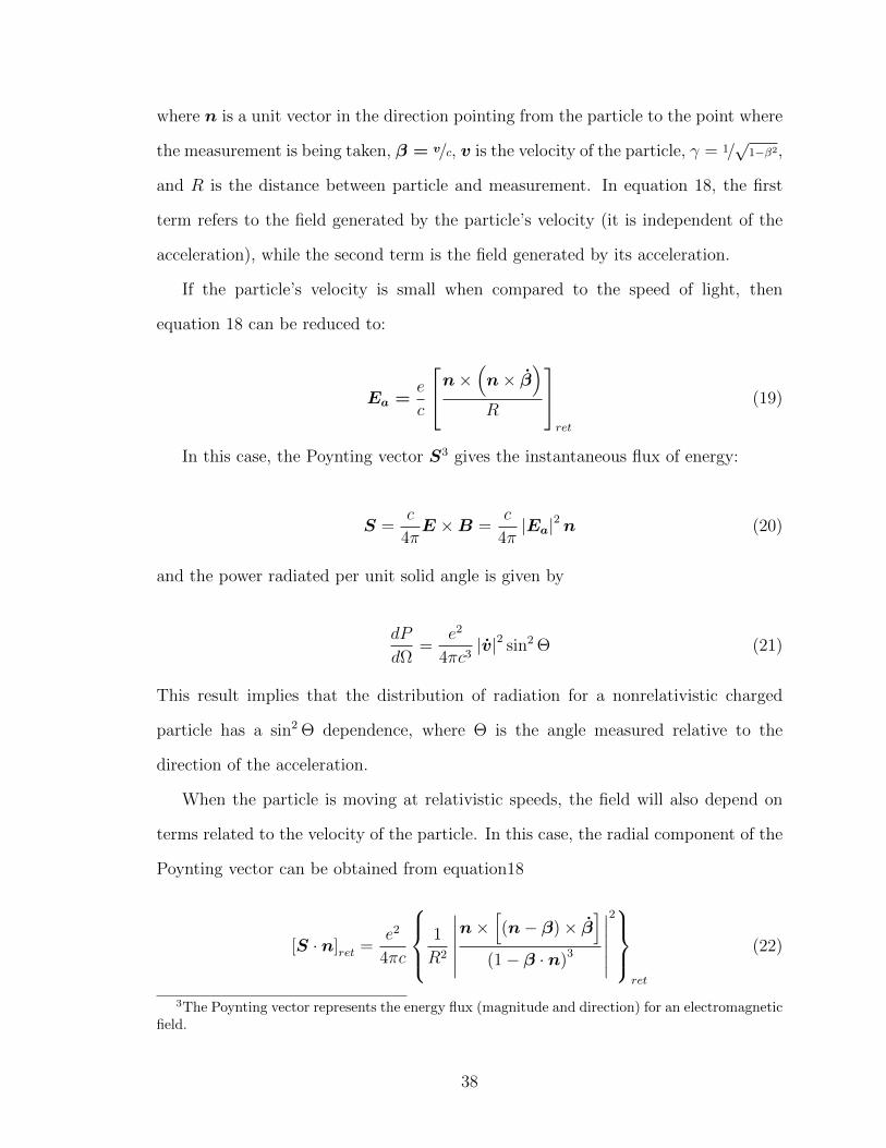
where n is a unit vector in the direction pointing from the particle to the point where
the measurement is being taken, β = v/c, v is the velocity of the particle, γ = 1/√
1−β2,
and R is the distance between particle and measurement. In equation 18, the first
term refers to the field generated by the particle’s velocity (it is independent of the
acceleration), while the second term is the field generated by its acceleration.
If the particle’s velocity is small when compared to the speed of light, then
equation 18 can be reduced to:
Ea =e
c
n×(n× β
)R
ret
(19)
In this case, the Poynting vector S3 gives the instantaneous flux of energy:
S =c
4πE ×B =
c
4π|Ea|2n (20)
and the power radiated per unit solid angle is given by
dP
dΩ=
e2
4πc3|v|2 sin2 Θ (21)
This result implies that the distribution of radiation for a nonrelativistic charged
particle has a sin2 Θ dependence, where Θ is the angle measured relative to the
direction of the acceleration.
When the particle is moving at relativistic speeds, the field will also depend on
terms related to the velocity of the particle. In this case, the radial component of the
Poynting vector can be obtained from equation18
[S · n]ret =e2
4πc
1
R2
∣∣∣∣∣∣n×
[(n− β)× β
](1− β · n)3
∣∣∣∣∣∣2ret
(22)
3The Poynting vector represents the energy flux (magnitude and direction) for an electromagneticfield.
38

while the power radiated per unit solid angle is defined as
dP (t′)
dΩ= R2S · n (1− β · n) (23)
Assuming that the particle is accelerated for only a small amount of time, such
that β and β can be considered constant in magnitude and direction, and that the
radiation is observed from far away, making n and R constant during the the particle
acceleration interval, then equation 23 can be rewritten as
dP (t′)
dΩ=
e2
4πc
∣∣∣n× (n− β)× β∣∣∣2
(1− n · β)5 (24)
where S · n was substituted from equation 22.
Taking the linear motion as an example (i.e., β and β are parallel), then
dP (t′)
dΩ=e2v2
4πc3
sin2 θ
(1− β cos θ)5 (25)
where θ is the angle measured from the direction of β and β. This result is the same
as the one in equation 21 for β 1 (i.e., for a nonrelativistic particle). If β → 1,
however, the angular distribution of the emitted radiation is tipped forward. The
radiation intensity is maximum at θmax, which is given by:
θmax = cos−1
[1
3β
(√1− 15β2 − 1
)](26)
This result shows that the angles at which most radiation is emitted by relativistic
particles are very small, and that the radiation is, thus, mostly emitted in a very
narrow cone around the direction of motion of the particles. It can be shown [121]
that this result is equivalent to the one for particles traveling in circular motion with
instantaneously constant speed, as is in the case of synchrotron sources.
In the case where β and β are perpendicular, such as in a synchrotron facility,
39

considering a coordinate system such that β is in the z direction and β is in the x
direction:
dP (t′)
dΩ=
e2
4πc3
|v|2
(1− β cos θ)3
[1− sin2 θ cos2 φ
γ2 (1− β cos θ)2
](27)
where θ and φ are the polar angles defining the direction of observation. In this case,
although the angular distribution is different than in the parallel case, the radiation
is also emitted in a narrow cone in the particle motion direction.
Appendix B explores the different devices used in synchrotron facilities to change
the direction of charged particles, causing their acceleration and the production of
synchrotron radiation. Appendix C discusses X-ray optics and interactions between
X-rays and matter, which are necessary to fully understand the techniques discussed
in sections 3.4 and 3.5.
3.4 X-ray fluorescence (XRF)
3.4.1 Theory and techniques
X-ray fluorescence measurements take into account the emission effects from the X-
ray interactions with matter to produce spectra (as discussed in Appendix C). The
energy of the peaks in the resulting spectrum can be associated with a chemical
element, according to their characteristic energy levels, and the peak intensity is
related to the quantity of the element in the sample [122].
In XRF analysis, the peaks are named according to the electron transition from
which they originate, as shown in fig. 2. Transitions to the K shell of the atom are
called Kα if the electron comes from the L shell, Kβ if the electron comes from the M
shell, and so on. Transitions to the L shell are called Lα (from M shell), Lβ (from the
N shell) and so on for other energy levels. In most XRF analysis, K and L transitions
are the most commonly visible [122].
40

Figure 2: Energy levels in an atom.
The next sections will discuss different ways of applying XRF in materials research,
such as spatially resolved XRF, XRF mapping and quantitative measurements.
Spatially resolved XRF Spatially resolved XRF refers to the control over the
area in the sample being measured in order to obtain the best conditions for the
experiment. Large excitation areas are usually used in homogeneous samples, when
there is no change in the element composition and concentration throughout the
sample. In this case, a large area in the sample is probed with limited need of
beam collimation, resulting in larger intensities and good statistics even for short
measurement times [123].
When using a smaller collimator, the probed area in the sample is smaller,
providing information on how the composition and concentration of elements change
spatially. The intensity of the beam is, however, lower in this case. Since the
intensity drops with the square of the spot diameter in collimators, there is a
limitation on how small the beam spot can be in order for enough statistics to be
41

obtained in a feasible amount of time [123].
If an even smaller beam spot is necessary, a different set of optics must be used.
An example is the polycapillary optics, which can provide a very small spot with
high flux. Very small spots are necessary to study very complex materials, such as
archaeological or geological samples [123].
In all the examples discussed so far, the size of the area studied depends on the
size of the beam spot on the sample. However, this is not the only way to control
how much of the sample is analyzed. A different approach is to shine radiation in a
large area of the sample and use a piece of X-ray optics (such as slits) between the
sample and the detector to select the fluorescence radiation produced in the desired
part of the sample. This approach requires that the incident radiation of very high
intensity, i.e., much higher than when using a collimated beam [123].
Another possible geometric arrangement for spatially resolved XRF involves the
use of the focusing optics. This can be used not only to collimate the beam, but
also to produce a confocal geometry. In this case, only the volume within the
intersection between both beam paths will be probed. Notice that, in the previous
examples, the collimation selects the area to be probed, but the depth is defined by
the characteristics of the radiation and sample material. In the confocal approach,
the method provides depth resolution as well, since it chooses a volume to be
probed [123].
A very common application of spatially resolved XRF is μ-XRF, where the beam
spot in the sample is on the order of micrometers. This technique can be used for
either single point measurements or to map larger areas in the sample [123].
XRF mapping XRF maps are single point measurements made in a grid, such
that the space between points either in the horizontal (x) or vertical (y) directions are
always the same (the distances do not need to be equal between the two directions).
42

In this case horizontal and vertical directions are perpendicular to each other and to
the direction of the beam propagation (z). The number of points in each direction,
and the space in between them (which will ultimately define the size of the map), are
decided according to the structure that is being measured [123].
A typical XRF map contains thousands of points. Even with very short
measurement times at each point, the time necessary to measure a complete map is
in the range of hours and depends on the experimental setup of the beamline: in
“stop-measure-go” setups, where the sample has to completely stop before data are
collected, the time consumed is much larger than in “on-the-fly” setups, where the
data are collected while the sample moves (and, therefore, the sample never stops)
[113]. The very short time spent in each point means that the intensity of the data
collected is very low, which necessitates very high beam intensity in experiments of
this kind [123].
The resulting data set provides information on the position of the measurement
(x and y in case a bidimensional map), on the energy E of the fluorescence photons,
and on the intensity I of fluorescence photons at a given energy by means of recording
a complete spectrum for each point (x, y) [123].
The data collected in a map is represented by a series of spectra, one for each
scanned point with fixed x and y coordinates. This allows to chemically characterize
spots and regions in the map. For example, specific regions of each spectrum,
representing a given chemical element, can be selected. The map can then be
showed applying this selection so that the distribution of this particular element can
be observed in the sample. Bidimensional distributions (x, y) of single or multiple
elements, or simply the selection of any given energy range, can be displayed this
way. In these distributions, a single chemical element map can be represented using
a colour scheme, where each colour corresponds to an intensity (obtained from the
integration under the area in the spectrum corresponding to this particular
43

element). If multiple elements are shown, they are usually each represented by a
different colour, while the intensity is represented by the colour’s brightness [123].
In order to analyze the data obtained in XRF maps, one must take into account the
experimental setup used and the possible detector artifacts that would influence the
element distribution in the map. The detectors normally used in XRF experiments,
as well as the possible detector artifacts present in the data collected, are discussed
in Appendix D.
3.4.2 Quantitative analysis
Qualitative analysis of XRF measurements can provide information on which elements
are present in the sample through simple visual analysis of the spectra. Another
qualitative method is the positive material identification (PMI), which compares the
measured spectrum with the spectra of known materials measured under the same
conditions for a fast identification [123].
Even though the qualitative analysis can provide valuable information about the
sample analyzed, quantitative analysis is also possible and often very accurate.
X-ray fluorescence has a very strong dependence on the sample’s matrix (i.e.,
measured intensities depend not only on the element concentration and
measurement conditions, but also on the other elements and geometry in the
sample). Therefore, calibration properties have to be changed for each sample, but
all the parameters are very well described by physical models [123]. The basic
physical model to describe how measured intensity is related to the weight fraction
is given by the Sherman equation:
Ii = G
ˆ
E
wiτi(E)S−1Spiωi
µ(E)sinψein
+ µ(i)sinψaus
I0(E)dE (28)
where Ii is the intensity of element i, G is a factor related to the geometry, w is
44
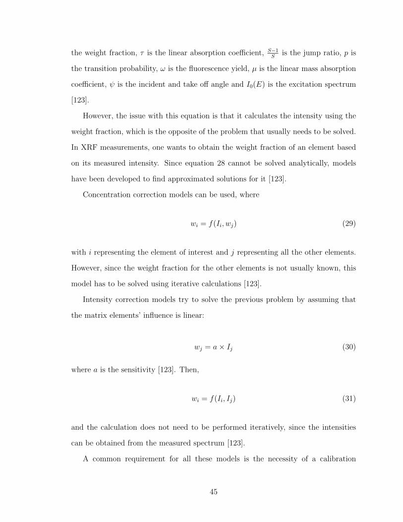
the weight fraction, τ is the linear absorption coefficient, S−1S
is the jump ratio, p is
the transition probability, ω is the fluorescence yield, µ is the linear mass absorption
coefficient, ψ is the incident and take off angle and I0(E) is the excitation spectrum
[123].
However, the issue with this equation is that it calculates the intensity using the
weight fraction, which is the opposite of the problem that usually needs to be solved.
In XRF measurements, one wants to obtain the weight fraction of an element based
on its measured intensity. Since equation 28 cannot be solved analytically, models
have been developed to find approximated solutions for it [123].
Concentration correction models can be used, where
wi = f(Ii, wj) (29)
with i representing the element of interest and j representing all the other elements.
However, since the weight fraction for the other elements is not usually known, this
model has to be solved using iterative calculations [123].
Intensity correction models try to solve the previous problem by assuming that
the matrix elements’ influence is linear:
wj = a× Ij (30)
where a is the sensitivity [123]. Then,
wi = f(Ii, Ij) (31)
and the calculation does not need to be performed iteratively, since the intensities
can be obtained from the measured spectrum [123].
A common requirement for all these models is the necessity of a calibration
45

procedure, which is used to find specific parameters of the measurement, such as
characteristics of the detector and beamline. The calibration is usually performed
using a sample with known weight fraction [123].
3.5 X-ray absorption fine structure (XAFS)
The X-ray Absorption Fine Structure (XAFS) spectrum provides information of the
local properties of the material being analyzed [116]. These spectra show a sharp
increase in the absorption when the energy of the incident X-rays correspond to
specific values characteristic for each element [124]. The energy values are determined
by the energy necessary for an electron in the atomic core to be ejected. The increases
in absorption are called edges and are named according to the original electronic level
of the ejected electron. In this way, the K-edge corresponds to electrons originating
from a 1s level and a L-edge corresponds to electrons originating from a 2s or 2p level
[124].
An incident X-ray beam is attenuated as it goes through a sample, which is given
by an exponential equation:
Φ = Φ0e−µ(ω)x (32)
where Φ and Φ0 are the beam flux (number of photons per unit time per unit
cross-section) after and before going through the sample, respectively, µ (ω)is the
attenuation coefficient as a function of the energy of the photons hω, and x is the
sample thickness [116]. As the energy of the incident photons increases, the
attenuation coefficient decreases and, thus, the resulting flux increases smoothly.
This behaviour is only different when the energy of the X-rays becomes high enough
that a core electron can be ejected and the absorption edge appears. Since the
energy necessary to eject a photoelectron from a determined shell increases with the
atom’s atomic number, its value is characteristic for each atomic species [116].
46

The edges present in the X-ray absorption fine structure provide information on
the local structure of the atom. In the case of isolated atoms, such as noble gases,
the fine structure is contained within a few eV around the edge and is the result
of the multiple allowed transitions to other bound levels in the atom, each with a
characteristic energy [116]. In more complex systems, however, the fine structure can
extend for hundreds of eV above the edge energy and it is influenced by the atoms
surrounding the absorber [116]. In this case, the XAFS can be divided into three
different regions, which provide different information about the absorber:
Pre-edge and edge. Limited to the region within a few eV from the edge. The
pre-edge is mostly the result of dipole allowed transitions to other bound states
and is most evident in oxides. It shows differences in the local structure well,
even if the atoms are in the same valence state [116]. The edge energy is related
to the oxidation state of the absorber (the higher the oxidation state, the higher
the edge energy). The shape of the edge is related to the geometry of the ligand
and can be used to identify specific chemical species [116, 124].
X-ray Absorption Near Edge Structure (XANES) or Near Edge X-ray
Absorption Fine Structure (NEXAFS). This is the region within ∼50 eV of
the edge and provides information on the electronic and geometric structures
around the absorber [116].
Extended X-ray Absorption Fine Structure (EXAFS). It is the region that
extends from the XANES region up to around a thousand eV above it. This
region provides information about the geometrical structure around the
atomic species being analyzed [116]. In this thesis, however, only the XANES
portion of the XAS spectrum was used and, therefore, the discussions that
follow will concentrate on this topic.
Although the interpretation of results obtained in the XANES region is more difficult
47

than the ones from the EXAFS region, the use of this technique has been increasing
in the past decades. This is due to several factors (when comparing to EXAFS),
such as the stronger spectral features, which makes interpretation less dependent on
statistics (and, therefore, beam intensity and quality of the sample). Consequently,
XANES is a very interesting choice for natural samples, which are very heterogenous,
or diluted samples. Other advantages are that XANES is subject to less temperature
effects than EXAFS, and that data acquisition is faster, which makes this technique
appropriate for time resolved measurements [116].
3.5.1 The XANES spectra
The analysis of XANES spectra, which typically includes the pre-edge, edge and post-
edge regions (fig. 3), provide information on the oxidation state and the environment
of the atoms [124], including their coordination chemistry, local structure and ligand
symmetry [116]. The different regions within XANES will be examined in more detail
in what follows.
Figure 3: Strontium XAFS spectrum with XANES region selected. Also representedthe different regions in XANES spectrum: pre-edge, edge and post-edge (multiplescattering region). (Original in colour) .
48

Edge The position of the edge provides information on the oxidation state of the
atom [116, 124]. This is due to the change in the energy necessary to excite an
electron when the total number of electrons in the atom changes. If the oxidation
state is higher, and, therefore, the number of electrons in the atom is smaller, the
overall charge of the atom is more positive and an electron will require more energy
to be excited away from its orbital [124]. Therefore, the higher the oxidation, the
higher the energy at which the edge appears [116, 124].
Pre-edge The pre-edge features are, mainly, the result of dipole allowed transitions
to other bound states in the atom [116]. For the K-edge in particular, the pre-edge is
mostly due to transitions from the 1s level to a level with p-symmetry (usually the first
available), which is a transition allowed by quantum mechanics (∆l = 1). Transitions
to levels with d-symmetry are not allowed (∆l = 2) and are rarer [116, 124]. They
can be detected in some cases, however, mainly when there is hybridization of p-d
levels [116].
Three types of transitions can be used to explain the features of pre-edges:
local electric quadrupole transitions (1s→ 3d);
non-local electric dipole transitions (1s → p), where the empty p states of the
absorber are hybridized with the empty d states of the neighbouring atoms;
local electric dipole transitions (1s → p), where the empty p states of the
absorber are hybridized with its empty d states.
Calculations can be used to determine the contribution of each type of transition to
the measured pre-edge [125].
Also, the position of the pre-edge can be used to fingerprint oxidation states for
some elements, such as iron, vanadium and chromium [125].
49

Post-edge The post-edge signal is the result of photoelectrons being excited to the
continuum states. The long mean free path for low energy electrons results in the
enhancement of multiple scattering terms (full multiple scattering, FMS), in contrast
to the EXAFS spectrum, which can be sufficiently explained using a single scattering
approximation (see section 3) [116]. By means of fittings and modeling, information
on local structure and coordination geometry can be obtained [116].
3.5.2 Qualitative and semi-quantitative analysis
The ab-initio calculation for XANES spectra can be very time consuming and requires
a very extensive knowledge of its theoretical background. Even though these methods
exist, others (qualitative and semi-quantitative) can be used to extract important
information without the need for a completely quantitative approach [116]. In the
next sections, some of these approaches will be explored.
Edge shift The edge shift method uses the position of the edge (or, in some cases,
pre-edge) to rapidly establish the oxidation state of a material. The energy of the
edge is compared to the energy of edges of known reference samples and the oxidation
state can be easily found [116].
Linear combination analysis (LCA) The linear combination analysis method
provides information on the relative amounts of different chemical species in a sample.
In order to do that, the normalized spectrum of the unknown sample µexp is fitted
with a linear combination of the spectra of reference compounds µth:
µexp =∑j
αjµth (33)
where aj represents the fraction of absorbers in the jth chemical state [116]. The
success of this method depends on having good-quality measurements for the
50

reference materials. Preferably, these measurements would be gathered as part of
the same experimental run as the measurements of the unknown sample, to prevent
measurement artifacts from interfering with the results [116].
This method is especially useful for heterogeneous samples, such as objects of
cultural relevance, biological specimens, and environmental science samples [116].
Principal component analysis (PCA) In the principal component analysis
approach, statistical considerations are used to select a set of spectra (principal
components) out of an ensemble of reference spectra, in order to perform a linear fit
on the data. This method is valuable for routine checks in large data sets, such as
for environment monitoring. However, one must be careful while selecting the
reference samples and check the final results so as to avoid non-physical answers
[116].
Deconvolution of XANES features The features seen around the edge region
on a XANES spectrum are due to very sharp peaks as a result of transitions to other
bound states in the atom over a smooth background of transitions to the continuum.
The distribution of peaks is related to the local symmetry and binding geometry in
the material. The analysis of these peaks, usually in comparison to references, can
be used to obtain information on coordination number and valence state of absorbers
[116].
3.5.3 Quantitative analysis
Theory The discussions in this section will follow reference [116].
X-ray absorption spectroscopy is studied in terms of the transitions between a core
state and an occupied level in an atom. The absorption coefficient µ (E)is written as
51

a function of the photon beam energy, and is given by
µ (E) = naσ (E) (34)
where na is the density of absorbers in the sample, and σ (E) is the local absorption
cross section, which can be calculated using Fermi’s “golden rule” with the dipole
approximation:
σ (ω) = 4π2α0~ω∑f
∣∣∣∣∣⟨
ΨNf
∣∣∣∣∣εN∑i=1
ri
∣∣∣∣∣ΨNg
⟩∣∣∣∣∣2
δ(~ω − EN
f + ENg
)(35)
where ε is the polarization vector for the incoming photon, ri indicates the position of
the ith electron and the initial and final states are many-body functions. This equation
considers all the possible excitations taking place in the atom and the creation of a
hole in the level φcL0with angular momentum L0 = (l0,m0).
The initial and final states can be approximately written, when spin variables are
omitted (i.e., for non-magnetic systems), as:
ΨNf (r, r1, ..., rN−1) =
√N !A
∑α
φfα (r) ΨN−1α (r1, ..., rN−1) (36)
where A is the anti-symmetrization operator, φfα are functions that describe the
excited photoelectron, and ΨN−1α are eigenstates of the Hamiltonian HN−1, which
describes the remaining N − 1 electrons and has eigenvalues EN−1α :
HN−1ΨN−1α = EN−1
α ΨN−1α . (37)
The tilde works as a reminder that the relaxed states around the core of the atom
are dominant in the expansion presented in equation 36.
Also, the eigenstate ΨNf of the total Hamiltonian HN has eigenvalues EN
f = ENg +
52
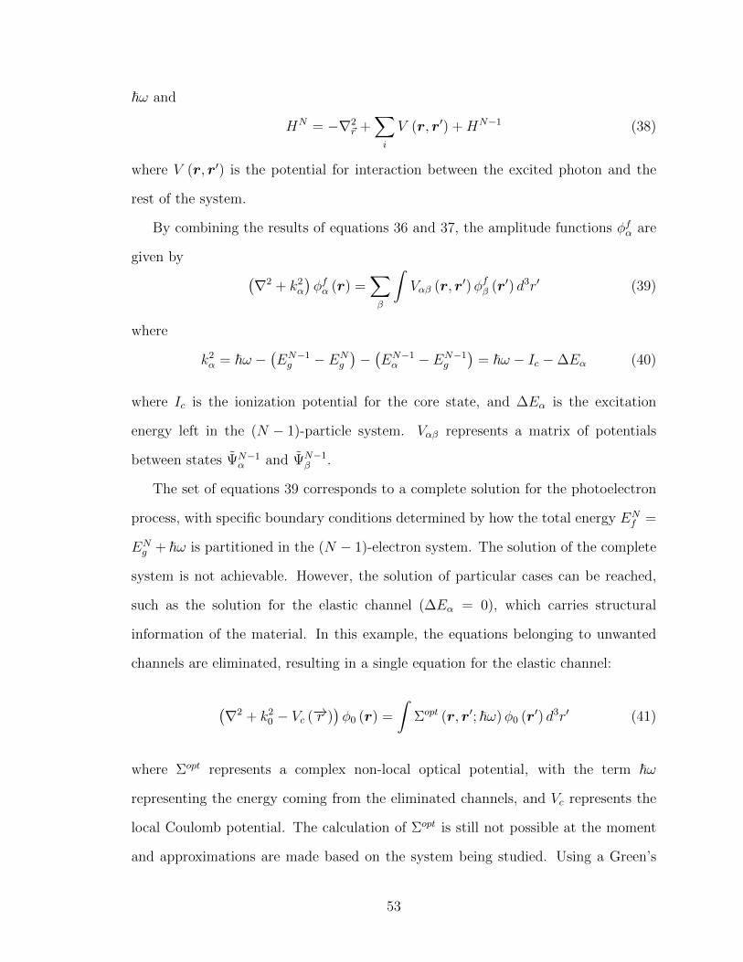
~ω and
HN = −∇2~r +
∑i
V (r, r′) +HN−1 (38)
where V (r, r′) is the potential for interaction between the excited photon and the
rest of the system.
By combining the results of equations 36 and 37, the amplitude functions φfα are
given by (∇2 + k2
α
)φfα (r) =
∑β
ˆVαβ (r, r′)φfβ (r′) d3r′ (39)
where
k2α = ~ω −
(EN−1g − EN
g
)−(EN−1α − EN−1
g
)= ~ω − Ic −∆Eα (40)
where Ic is the ionization potential for the core state, and ∆Eα is the excitation
energy left in the (N − 1)-particle system. Vαβ represents a matrix of potentials
between states ΨN−1α and ΨN−1
β .
The set of equations 39 corresponds to a complete solution for the photoelectron
process, with specific boundary conditions determined by how the total energy ENf =
ENg + ~ω is partitioned in the (N − 1)-electron system. The solution of the complete
system is not achievable. However, the solution of particular cases can be reached,
such as the solution for the elastic channel (∆Eα = 0), which carries structural
information of the material. In this example, the equations belonging to unwanted
channels are eliminated, resulting in a single equation for the elastic channel:
(∇2 + k2
0 − Vc (−→r ))φ0 (r) =
ˆΣopt (r, r′; ~ω)φ0 (r′) d3r′ (41)
where Σopt represents a complex non-local optical potential, with the term ~ω
representing the energy coming from the eliminated channels, and Vc represents the
local Coulomb potential. The calculation of Σopt is still not possible at the moment
and approximations are made based on the system being studied. Using a Green’s
53
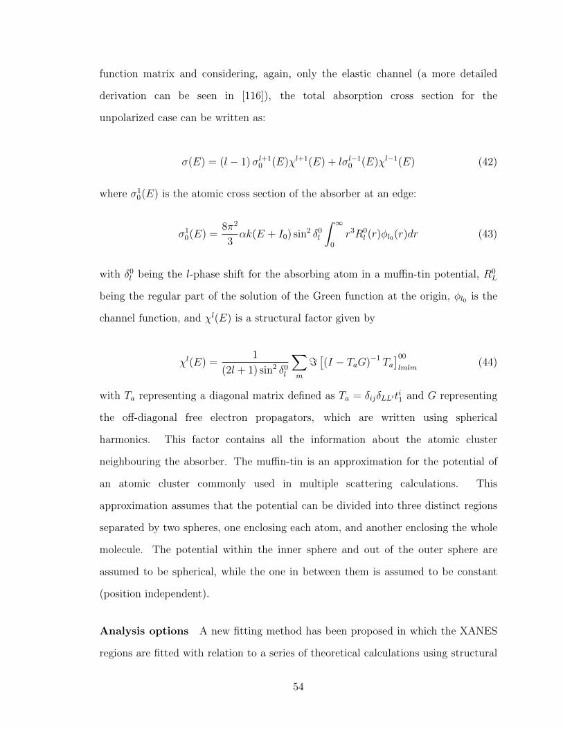
function matrix and considering, again, only the elastic channel (a more detailed
derivation can be seen in [116]), the total absorption cross section for the
unpolarized case can be written as:
σ(E) = (l − 1)σl+10 (E)χl+1(E) + lσl−1
0 (E)χl−1(E) (42)
where σ10(E) is the atomic cross section of the absorber at an edge:
σ10(E) =
8π2
3αk(E + I0) sin2 δ0
l
ˆ ∞0
r3R0l (r)φl0(r)dr (43)
with δ0l being the l-phase shift for the absorbing atom in a muffin-tin potential, R0
L
being the regular part of the solution of the Green function at the origin, φl0 is the
channel function, and χl(E) is a structural factor given by
χl(E) =1
(2l + 1) sin2 δ0l
∑m
=[(I − TaG)−1 Ta
]00
lmlm(44)
with Ta representing a diagonal matrix defined as Ta = δijδLL′ti1 and G representing
the off-diagonal free electron propagators, which are written using spherical
harmonics. This factor contains all the information about the atomic cluster
neighbouring the absorber. The muffin-tin is an approximation for the potential of
an atomic cluster commonly used in multiple scattering calculations. This
approximation assumes that the potential can be divided into three distinct regions
separated by two spheres, one enclosing each atom, and another enclosing the whole
molecule. The potential within the inner sphere and out of the outer sphere are
assumed to be spherical, while the one in between them is assumed to be constant
(position independent).
Analysis options A new fitting method has been proposed in which the XANES
regions are fitted with relation to a series of theoretical calculations using structural
54
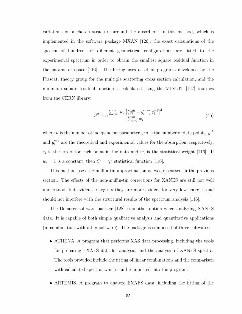
variations on a chosen structure around the absorber. In this method, which is
implemented in the software package MXAN [126], the exact calculations of the
spectra of hundreds of different geometrical configurations are fitted to the
experimental spectrum in order to obtain the smallest square residual function in
the parameter space [116]. The fitting uses a set of programs developed by the
Frascati theory group for the multiple scattering cross section calculation, and the
minimum square residual function is calculated using the MINUIT [127] routines
from the CERN library:
S2 = n
∑mi=1 wi
[(ythi − y
expi
)ε−1i
]2∑mi=1wi
(45)
where n is the number of independent parameters, m is the number of data points, ythi
and yexpi are the theoretical and experimental values for the absorption, respectively,
εi is the errors for each point in the data and wi is the statistical weight [116]. If
wi = 1 is a constant, then S2 = χ2 statistical function [116].
This method uses the muffin-tin approximation as was discussed in the previous
section. The effects of the non-muffin-tin corrections for XANES are still not well
understood, but evidence suggests they are more evident for very low energies and
should not interfere with the structural results of the spectrum analysis [116].
The Demeter software package [128] is another option when analyzing XANES
data. It is capable of both simple qualitative analysis and quantitative applications
(in combination with other software). The package is composed of three softwares:
ATHENA. A program that performs XAS data processing, including the tools
for preparing EXAFS data for analysis, and the analysis of XANES spectra.
The tools provided include the fitting of linear combinations and the comparison
with calculated spectra, which can be imported into the program.
ARTEMIS. A program to analyze EXAFS data, including the fitting of the
55
spectra.
HEPHAESTUS. A program that contains tools based on the periodic table
and absorption cross sections for various elements. Among other tools, it can
display absorption and fluorescence line energies and other relevant chemical
information for the elements and show charts containing the transitions
associated with absorption lines [128].
The FEFF9 [129] is a code with user interface used to calculate XAS spectra using
Green’s functions. Details of how the calculations are performed as well as examples
can be seen in [129].
3.6 Conclusions
The use of synchrotron radiation in characterization techniques provides results with
high resolution and statistics, and requires short acquisition times when compared
to other light sources. This characteristic is essential to the application of such
techniques to palaeontology due to the heterogeneity in the composition of specimens.
Palaeontological samples have a large quantity of different elemental or molecular
species, some of which appear in very low concentrations.
Synchrotron XRF can be used to detect heterogeneities and the distribution of
elements at microscopic level. This makes the detailed analysis of the chemical
composition and of correlations between elements in fossils possible. XRF can also
be used to detect the presence of trace elements. However, the information obtained
in most palaeontologic situations is qualitative. Although quantitative
measurements can be done with this technique, these become particularly difficult
to apply to fossils. Among other factors, fossils usually present irregular surfaces
(e.g., due to the presence of canals in bones), resulting in geometric effects on the
measurements, which would have to be considered in a quantitative analysis. Even
56

with these limitations, the technique is very useful to study chemical properties of
fossils, such as diagenetic alterations, in the specimens.
While XRF provides information about different chemical elements, XAFS studies
their speciation into different compounds and chemical states. This technique can be
used to identify characteristics such as the oxidation state, the compound the element
belongs to, and mixtures of states. The application of XAFS to palaeontology can be
used to suggest the origin of different elements in samples (i.e., biologic or diagenetic),
or the path that led to the specimen’s preservation.
57

4 Chemical diagenesis of Tyrannosaurus rex
bones from the Frenchman Formation
4.1 Abstract
Tyrannosaurus rex is one of the most widely recognised dinosaur species, probably
because of its large size and strength. Among the fossils found for members of this
species, there is a relatively complete skeleton (informally known as “Scotty”) that
was found in the Frenchman River Valley (Saskatchewan, Canada) in 1991
[140].“Scotty” is noteworthy because of the large percentage of bones found, which
represent approximately 65% of the skeleton. These have preserved microstructures
visible, for instance, using optical microscopes, among other techniques; and some of
its features can be analyzed through petrographic techniques, such as the one to be
discussed in section 4.4.
The goals of this study include the exploration of diagenetic changes and
taphonomic history of this specimen. This is accomplished by comparing the
chemical analysis of its bones to other bones found in the same stratigraphic
interval and geographic region, and a modern (extant) swan is used as a control
sample. Another goal is the establishment of a hypothesis to partially explain its
preservation.
The results obtained (section 4.4) show that the T. rex bones were considerably
altered diagenetically, mainly by the addition of yttrium and strontium in the bone
tissue, and the presence of a layer of manganese in the transition region between the
bone surface and the associated sediment matrix. The manganese layer indicates that
the T. rex ’s tissues were exposed to an aquatic environment where manganese was
present, probably as oxides or hydrates. The presence of Fe(III) in the bone tissue
offers hints about why this specimen was preserved (see section 2.4.2), and fine details
of the diagenetic changes observed.
58
4.2 Introduction
The first members of the clade Dinosauria probably appeared during Early to
Middle Triassic. However, the oldest known specimens date back to the Late
Triassic, during the Carnian age (˜228 to ˜216.5 Ma) [141]. The members of this
clade can be classified into two orders: Saurischia and Ornithischia, named after
differences in their hip structures. The dinosaurs belonging to the order Saurischia
can be divided into two suborders: Sauropodomorpha, which will not be described
here (see [143] and [144]) and Theropoda (“beast-footed ones”) [145]. The
Theropoda are widely known for containing large predators, such as Spinosaurus,
Giganotosaurus and Tyrannosaurus. However, the group also contained species of
omnivores and herbivores, as well as dinosaurs among the smallest present in the
Mesozoic, such as Epidendrosaurus, Microraptor and Mei [145]. Theropods can be
considered the most successful group of dinosaurs, as they were the only dinosaurs
to survive the catastrophic extinction event at the end of the Cretaceous, in the
form of birds (Aves) [145]. They were strict bipeds and most of them were
characterized by ziphodont teeth, long grasping hands with recurved claws (that
were usually sharp), chambers and openings in the skull bones associated with air
sacs and hollow limb bones and vertebrae [145].
Tyrannosauroidea (tyrant dinosaurs) are a group of theropods best known for
their Late Cretaceous members found in Asia and North America, belonging to the
family Tyrannosauridae. The early members of Tyrannosauroidea evolved fused
nasals, which allowed for a stronger bite, incisiform premaxillary teeth, and a
narrow metacarpal III [145]. Tyrannosauridae, in particular, appeared in the Late
Cretaceous and were the largest predators in their environments, with most species
reaching at least 10 m in length. They were characterized by having large and wide
skulls, which allowed for forward-facing eyes (binocular vision); a thick maxillary,
and teeth with long roots (which were probably capable of crushing through bone);
59

large neck muscle attachments; and short forelimbs with didactyl hands [145].
Tyrannosaurids probably depended on their jaws as a primary tool for hunting, and
their long legs allowed for fast running — at least for the lighter members of the
group and juveniles. Among tyrannosaurids, one can find the genus Tyrannosaurus
and the species Tyrannosaurus rex, which represented the largest predator in
western North America in its time [145].
As organs, bones are responsible for the support and protection of the organs
and tissues in the body, metabolic control of mineral homeostasis, and housing the
bone marrow, which is involved in the production of blood cells. Bones also provide
attachment points for muscles, ligaments and tendons, and store calcium and
phosphate in the body [146].
Bones are composed of organic and mineral components [147]. The organic
components form a framework for the mineralization to occur, and provide tensile
strength and elasticity to the bone. The main organic component of bone is type I
collagen, a triple helix-shaped protein made of two collagen α1 (I) peptide chains
and one collagen α2 (I) peptide chain [147]. Bones also contain other types of
collagen, non-collagenous proteins (e.g., fibronectin, osteocalcin), and other organic
molecules [147]. The mineralization of the bone confers its mechanical rigidity. The
main mineral components are calcium and phosphate in the form of hydroxyapatite
(Ca10(PO4)6(OH2)) crystals [147], although other elements chemically similar to
calcium such as strontium and barium can also be found in bone apatite [148].
Bone tissue can be classified into compacta or spongiosa, according to its porosity.
The tissue is considered compacta when its mineral volume is larger than the empty
volume found in its pores, and spongiosa otherwise [146]. In general, compacta tissue
can be found in the outer cortex of bones and spongiosa tissue can be found in its
center (although that is not always the case) [146]. Bones (except their joints) are
usually covered by the periosteum [149, 150]. This membrane is important to the
60

modelling and remodelling of bone, particularly when repairing fractures [149, 151].
Bone tissues can also be classified according to their structural patterns. These
patterns include: lamellar bone, where the tissue consists of thin layers with high
density of collagen fibers; woven-fiber bone, where the tissue is composed of
disorganized collagen fibers of different sizes with varying orientations; and
parallel-fibered bone, where the tissue is composed of a parallel arrangement of
tightly packed collagen fibers [146].
The bones are supplied with blood through Harvesian canals, which run the length
of the bone (fig. 4), and Volkmann’s canals, which exhibit radial orientation and
connect different Havesian canals [146]. When bone is formed or grows, the blood
vessels are incorporated in large canals formed by the deposition of matrix around
them. These canals can be later filled by concentric deposition of lamellar tissue and
these structures (i.e., blood vessels surrounded by lamellar tissue) form what is known
as primary osteons (fig. 4). Secondary osteons are the result of changes in the bone
during the animal’s life, where bone tissue can be reabsorbed and re-metabolized
around a blood vessel, which is, then, surrounded by concentric layers of lamellar
tissue [146].
Figure 4: “Bone anatomy”. Modified from [139]. Licenced under the terms andconditions of the Creative Commons Attribution (CC BY). (Original in colour).
The application of synchrotron techniques such as the ones used in this research to
61
the study of fossils is a relatively recent advancement. It has only become more widely
known and used after results were obtained for the primitive bird Archaeopteryx [152]
in the early 2010s. In that study [152], synchrotron rapid scanning X-ray fluorescence
was used to chemically analyze feathers. It showed that these feathers were not just
impressions, as it was once believed, but instead were fossilized structures with a
chemical composition different from the surrounding material. The use of synchrotron
techniques in paleontology (and archeology) studies has been reviewed in [153].
In general, synchrotron X-ray techniques are applied to fossils with the goals of 1)
restoring lost information, such as the behaviour and biology of extinct animals; 2)
understanding the taphonimic processes that fossils go through, so that it is possible
to recreate the original (and lost) information about the material; and 3) predicting
the chemical pathways similar objects would follow, making it possible to prevent
further damages to the specimens already in collection [153, 154]. These techniques
have shown that the materials found in fossil bones are chemically different from the
sedimentary matrix where they are found, suggesting that although altered, their
chemical information is not completely lost due to diagenesis [155].
Some examples of work developed using synchrotron techniques to study dinosaur
bones include the use of synchrotron XRF to map chemical difference between healthy
and pathological bone for extant and extinct archosaurs (see section 2.4.1 for bone
preservation studies that do not involve synchrotron radiation). This work showed
specific features in the regions between different types of bone, like compact and
spongy bone, as well as the presence of zinc as a possible biomarker for ossification
processes [156]. Another study used a combination of synchrotron XRF for high
atomic number (Z) elements, and energy-dispersive X-ray spectroscopy (EDX) for low
Z elements, to chemically map the distribution of trace elements in sauropod bones in
order to identify the effects of diagenesis. This research showed that even bones that
did not show considerable changes at the histological level presented a considerable
62

degree of diagenetic alteration, including cracks and the presence of mineral filling in
pores and canals [157]. Synchrotron XRF, scanning electron microscopy (SEM), and
XAFS were also used in [158] to study bones of an artiodactyl and a perissodactyl from
Greece. They mapped the distribution of bone apatite using the presence of calcium
and phosphorous, and identified oxides with iron filling cavities in the bones. Goethite
and pyrite were detected in the samples, and strontium was found to substitute for
calcium in the bone apatite. Manganese was also detected in considerable amounts
close to cracks, and contaminating the periosteum and medullar cavity.
XRF (not using synchrotron radiation), in combination with other techniques
(X-ray diffraction and Fourier transform infrared spectroscopy), have also been used
to characterize diagenetic alterations in the bones of Upper Jurassic/Lower
Cretaceous to Upper Cretaceous dinosaurs from Spain in [159]. This study detected
large amounts of calcium, phosphorus, iron and strontium in the bones, along with
the presence of goethite (FeOOH) and celestite (SrSO4) phases. This study was also
able to identify elements with higher atomic number (Y, As, Pb, Ti, Mn, Cr, Cu,
Zn) in trace amounts.
4.2.1 Scotty, the Saskatchewan T. rex
The Tyrannosaurus rex specimen (RSKM P2523.8) analyzed herein is informally
known as “Scotty”, and was found in the Frenchman River Valley, close to the town
of Eastend in Saskatchewan (Canada), in 1991. However, it was only fully identified
in 1994, in the same year that large-scale excavations started [140]. The skeleton
was not articulated and was partially encased in a mixture of ironstone and very
well-cemented sandstone. Both these matrices made the excavation process more
laborious, necessitating two complete summers of fieldwork to extract the specimen
[140].
“Scotty” was found in the Frenchman Formation, the youngest Cretaceous
63

formation in southwestern Saskatchewan [160], dated to the Late Maastrichtian
[161]. The formation is a sedimentary succession stratigraphically located between
the underlying Battle Formation and the overlying Ravenscrag Formation
[162, 163, 164]. Due to the Battle Formation having been eroded in some areas, or
not deposited at all in other areas [161], the Frenchman Formation can appear on
top of the Bearpaw, Eastend or Whitemud formations in different regions of
Saskatchewan [165, 166, 167]. The contact between the Frenchman and Ravenscrag
formations is usually conformable, presenting a continuous deposit over the
Cretaceous-Paleogene boundary [161]. This transition is rich in iridium and has
been interpreted as a result of the meteorite impact event linked to the K-Pg mass
extinction [168, 169, 170].
The thickness of the Frenchman Formation varies from 8.5 m to more than 67.7 m,
increasing in thickness heading outward from the town of Eastend in both northern
and eastern directions [167]. The formation is composed of laterally discontinuous
layers of two different facies, one of these is mostly composed of sand, and the other
is mostly composed of clay [161, 163, 167]. The sandy facies are predominantly
formed by medium-to-fine grained subgreywackes cemented by calcium carbonate
[163], forming large sandstone masses in some regions [167]. The clay facies, however,
are composed of bentonitic clays, which exhibit a popcorn-like surface when dry [163].
The T. rex skeleton found in the Frenchman Formation and described in the next
section was found in sediments of the sandy facies [161].
The RSKM P2523.8 skeleton discussed in this thesis is one of the most massive
specimens found to date, measuring almost 12 metres in length and 4 metres in height,
with an estimated weight of 6 tonnes [171]. The specimen is also unique in having
been found in association with preserved seeds, leaves, fruits and other plant remains
[161]. The presence of plant and animal fossils in the same area is a rare taphonomic
event due to differences in conditions required for the preservation of bone and plant
64
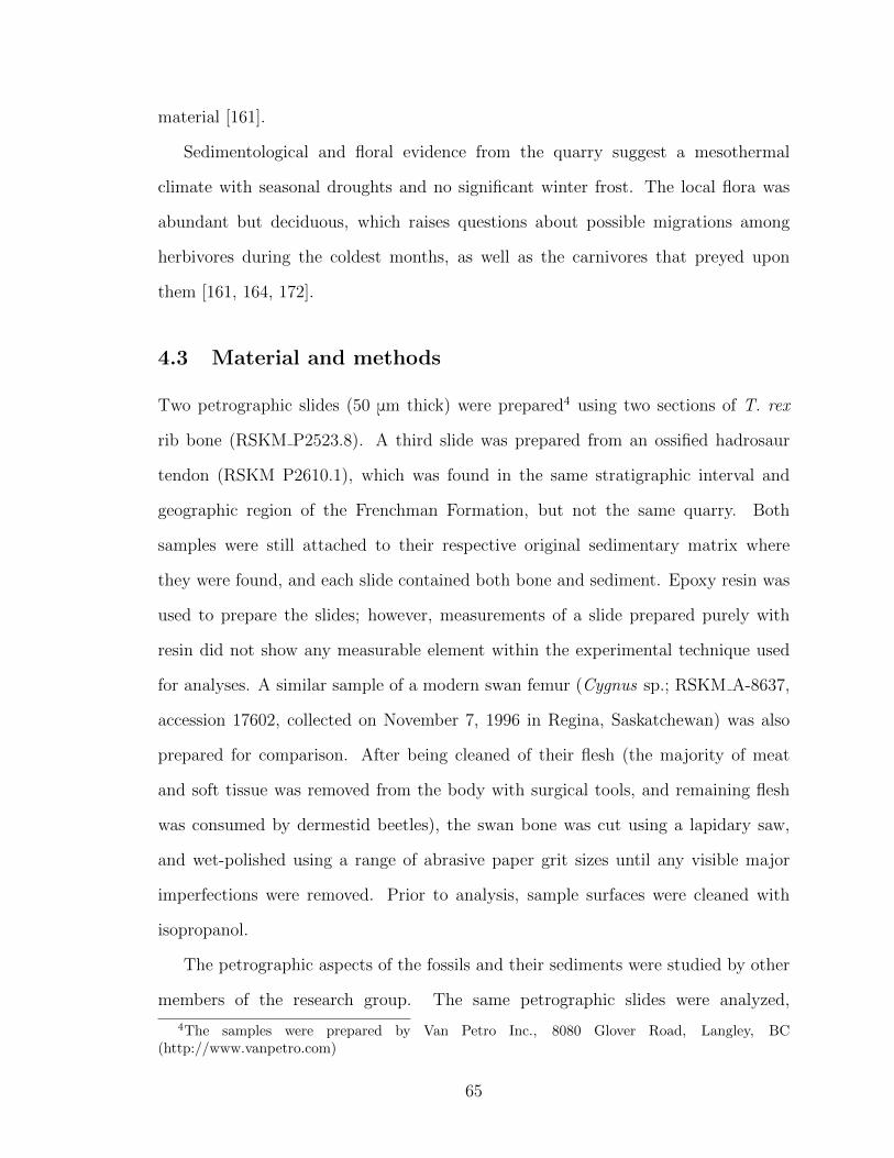
material [161].
Sedimentological and floral evidence from the quarry suggest a mesothermal
climate with seasonal droughts and no significant winter frost. The local flora was
abundant but deciduous, which raises questions about possible migrations among
herbivores during the coldest months, as well as the carnivores that preyed upon
them [161, 164, 172].
4.3 Material and methods
Two petrographic slides (50 μm thick) were prepared4 using two sections of T. rex
rib bone (RSKM P2523.8). A third slide was prepared from an ossified hadrosaur
tendon (RSKM P2610.1), which was found in the same stratigraphic interval and
geographic region of the Frenchman Formation, but not the same quarry. Both
samples were still attached to their respective original sedimentary matrix where
they were found, and each slide contained both bone and sediment. Epoxy resin was
used to prepare the slides; however, measurements of a slide prepared purely with
resin did not show any measurable element within the experimental technique used
for analyses. A similar sample of a modern swan femur (Cygnus sp.; RSKM A-8637,
accession 17602, collected on November 7, 1996 in Regina, Saskatchewan) was also
prepared for comparison. After being cleaned of their flesh (the majority of meat
and soft tissue was removed from the body with surgical tools, and remaining flesh
was consumed by dermestid beetles), the swan bone was cut using a lapidary saw,
and wet-polished using a range of abrasive paper grit sizes until any visible major
imperfections were removed. Prior to analysis, sample surfaces were cleaned with
isopropanol.
The petrographic aspects of the fossils and their sediments were studied by other
members of the research group. The same petrographic slides were analyzed,
4The samples were prepared by Van Petro Inc., 8080 Glover Road, Langley, BC(http://www.vanpetro.com)
65

alongside the other dinosaur sample and the swan sample, at the VESPERS (Very
Sensitive Elemental and Structural Probe Employing Radiation from a Synchrotron)
beamline at the Canadian Light Source (CLS) using micro-XRF mapping and
XANES techniques [173]. VESPERS is a bending magnet beamline, with an energy
ranging between 6 and 30 keV and spot size of 2 to 4 μm, produced by KB mirrors
[173]. The XRF measurements were taken using a polychromatic beam, while
XANES measurements for strontium were collected in fluorescence mode using a
monochromatic beam produced by a crystal and multilayer monochromator.
Data previously taken by other members of the research group from a vertebra
of RSKM P2523.8 were also analyzed. The vertebra sample was prepared by cutting
with a water-cooled saw to expose a section of the bone, and cleaned with ethanol.
The measurements were also performed at the VESPERS (XRF) and SXRMB
(XANES in fluorescence mode for iron, sulfur and calcium) [174] beamlines at the
CLS. SXRMB (Soft X-ray Microcharacterization Beamline) is also a bending
magnet beamline providing medium energy X-rays (1.7 to 10 keV) that can be used
for X-ray photoelectron spectroscopy (XPS), X-ray absorption spectroscopy (XAS)
and elemental mapping using XRF. The photon beam energy is selected using a
double crystal monochromator with InSb(111) crystals for energies below 3.7 keV
and Si(111) crystals for higher energies. The beam collimation is achieved by a
sagittal cylindrical mirror with a carbon and platinum bi-layer coating.
The elements calcium, iron, manganese, strontium and yttrium were chosen for
the analysis using XRF because they are present in non-negligible amounts in all
fossil samples studied. These elements have also been previously researched in the
context of fossil bones (see section 4.2). The XRF data were analyzed using PyMCA
software [175], developed by scientists from the European Synchrotron Radiation
Facility (ESRF). This software allows for peak finding and fitting, and chemical
element map reconstruction based on the selection of regions of interest (ROIs) for
66

each element, once energy calibration is performed. The maps are produced in RGB
(red - green - blue) colours and can be plotted together in the same picture for
comparison. The average spectra for the bone regions in each of the samples was
also computed. For that, 800 pixels of the compact bone region in each sample were
selected, their spectra were averaged, and then normalized (for each spectrum, each
point was divided by the highest count value in the spectrum, ynorm = yymax
).
PyMCA was also used to open and convert XANES data to a format that the
software Athena could read for data analysis. This software is present in the Demeter
package [176], which contains three programs related to XAS analysis. The data were,
then, normalized using the standard method in Athena to eliminate the influence of
factors such as sample thickness and detector settings. In the case of iron XANES
K-edge measurements, the pre-edge was later fitted using the software Larch [177],
with an error function given by:
erf(x) =1√π
xˆ
−x
e−t2
dt =2√π
xˆ
0
e−t2
dt, (46)
to fit the edge component and a pseudo-voigt function to fit the pre-edge. The
pseudo-voigt function is defined as
f(x;A, µ, σ, α) =(1− α)A
σg√
2πe
[−(x−µ)2
2σ2g
]+αA
π
[σ
(x− µ)2 + σ2
], (47)
which is a weighted sum of a Gaussian and a Lorentzian distribution (weight given by
α) sharing the same amplitude, A, center, µ, and the same full width at half maximum,
thus constraining the parameter σ. For the fittings presented here, α = 0.5.
4.4 Results
The petrographic description of the slides containing T. rex (RSKM P2523.8) and
hadrosaur (RSKM P2610.1) shows significant of quartz and plagioclase in the
67

sediment surrounding all three samples. Both T. rex slides present lithic grains and
muscovite. The bone in the T. rex samples contains osteons with preserved
diameters between 0.5 and 1 mm, and with areas that exhibit a silver sheen due to
alterations around fractures and between the circular patterns of osteons. The
hadrosaur ossified tendon presents osteons with Harvesian canals of 0.1 to 0.5 mm
in diameter, with alterations around the perimeter of bone and osteons. All
measurements presented in this chapter were taken on regions of compact bone (fig.
5) showing microscope images of the samples studied herein, and the general regions
mapped.
Figure 5: Miscroscope images of a) T. rex rib (RSKM P2523.8), b) T. rexrib (RSKM P2523.8), c) T. rex vertebra (RSKM P2523.8), d) hadrosaur tendon(RSKM P2610.1), and e) swan femur (RSKM A-8637). Braces show the generalregion mapped in each sample, which corresponds in all fossils to the region in theinterface between bone and sedimentary matrix. Blue arrows show the region withbone, while red arrows shows regions with sedimentary matrix in the samples. Thescale bars correspond to 3 mm. (Original in colour)
XRF maps of two slides of RSKM P2523.8 T. rex rib bones and vertebra are
presented in fig. 6, 7 and 8, respectively. In all samples, the bone region is still
68
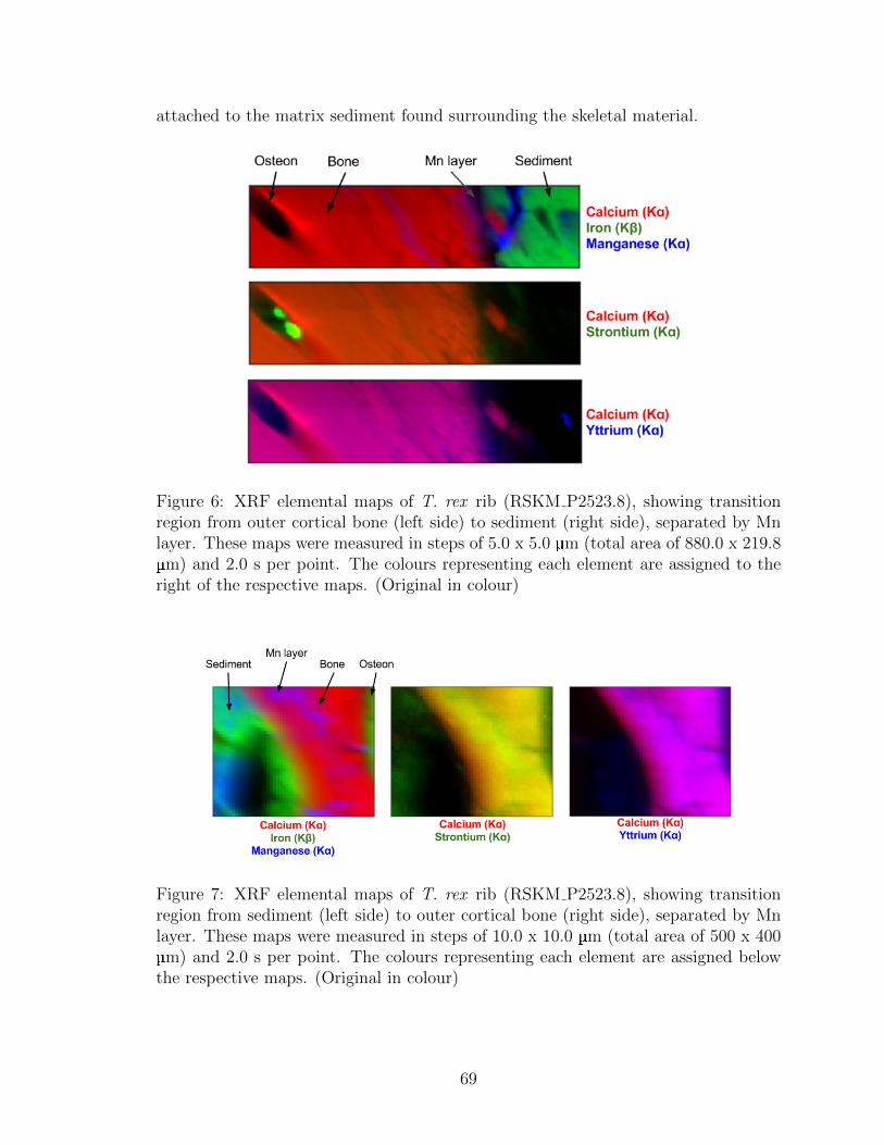
attached to the matrix sediment found surrounding the skeletal material.
Figure 6: XRF elemental maps of T. rex rib (RSKM P2523.8), showing transitionregion from outer cortical bone (left side) to sediment (right side), separated by Mnlayer. These maps were measured in steps of 5.0 x 5.0 µm (total area of 880.0 x 219.8µm) and 2.0 s per point. The colours representing each element are assigned to theright of the respective maps. (Original in colour)
Figure 7: XRF elemental maps of T. rex rib (RSKM P2523.8), showing transitionregion from sediment (left side) to outer cortical bone (right side), separated by Mnlayer. These maps were measured in steps of 10.0 x 10.0 µm (total area of 500 x 400µm) and 2.0 s per point. The colours representing each element are assigned belowthe respective maps. (Original in colour)
69

Figure 8: XRF elemental maps of T. rex vertebra (RSKM P2523.8), showingtransition region from sediment (bottom) to outer cortical bone (top). These mapswere measured in steps of 20.0 x 20.0 µm (total area of 900 x 2100 µm) and 5.0 s perpoint. The colours representing each element are assigned below the respective maps.(Original in colour)
The elemental maps in figs. 6-8 show a very similar pattern in the distribution of
the elements for the three specimens. Calcium appears mostly in the region where
bone is present, marking even some of its microstructure (see Harvesian canal in
fig. 6). Strontium and yttrium are distributed in the same general region where
calcium is present, but also in the areas immediately surrounding these regions, and
in cracks and canals (e.g., fig. 8). Iron is present mostly in the regions corresponding
to sedimentary matrix and within the osteon canal in fig. 7. Manganese appears in
the transition between bone and sedimentary matrix.
The results of the data analysis for the hadrosaur tendon and extant swan bone
are presented in figs. 9 and 10, respectively.
70

Figure 9: XRF elemental maps of hadrosaur tendon (RSKM P2610.1), showingtransition from bone (top) to sediment (bottom). These maps were measured insteps of 5.0 x 5.0 µm (total area of 700 x 750 µm) and 2.0 s per point. The coloursrepresenting each element are assigned below their respective maps. (Original incolour)
Figure 10: XRF elemental maps of recent swan femur cortical bone (RSKM A-8637).These maps were measured in steps of 5.0 µm (total area of 400 x 300 µm) and 2.0 sper point. The colours representing each element are assigned below their respectivemaps. (Original in colour)
The distributions of calcium, iron, strontium, and yttrium observed for
RSKM P2610.1 in fig. 9 are very similar to what was observed in the Tyrannosaurus
bones. The main difference is the manganese distribution, which instead of marking
71
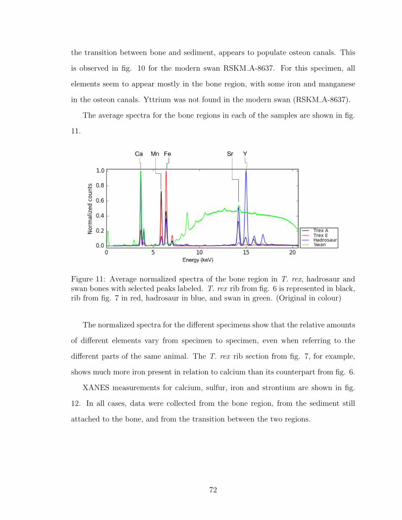
the transition between bone and sediment, appears to populate osteon canals. This
is observed in fig. 10 for the modern swan RSKM A-8637. For this specimen, all
elements seem to appear mostly in the bone region, with some iron and manganese
in the osteon canals. Yttrium was not found in the modern swan (RSKM A-8637).
The average spectra for the bone regions in each of the samples are shown in fig.
11.
Figure 11: Average normalized spectra of the bone region in T. rex, hadrosaur andswan bones with selected peaks labeled. T. rex rib from fig. 6 is represented in black,rib from fig. 7 in red, hadrosaur in blue, and swan in green. (Original in colour)
The normalized spectra for the different specimens show that the relative amounts
of different elements vary from specimen to specimen, even when referring to the
different parts of the same animal. The T. rex rib section from fig. 7, for example,
shows much more iron present in relation to calcium than its counterpart from fig. 6.
XANES measurements for calcium, sulfur, iron and strontium are shown in fig.
12. In all cases, data were collected from the bone region, from the sediment still
attached to the bone, and from the transition between the two regions.
72

Figure 12: XANES measurements for a T. rex bone (RSKM P2523.8) still attachedto its surrounding sediment for a) calcium, b) sulfur, c) iron and d) strontium. Arrowsshow some of the regions of the spectra where differences between measurements canbe seen. (Original in colour).
The measurements for calcium (fig. 12-a) show that two very distinct chemical
states for this element are present in the bone and sediment, with an intermediate
state in the transition region. This difference is best seen in the plot areas marked by
the arrows in fig. 12. The spectra for sulfur in fig. 12-b shows the peak position for
all measurements at ∼ 2481.7 eV. However, the chemical state does not seem to be
the same for all regions (see feature marked by the arrow in the pre-edge region, for
example). The spectra for strontium (fig. 12-d) are slightly different for the different
regions in the sample.
The iron K-edge measurements (fig. 12-c) show very different spectra for bone and
sediment. The results of the fitting in the pre-edge portions of these spectra can be
seen in figs. 13, 14, and 15, for the bone, transition area, and sediment, respectively.
73

The fitting of the spectra resulted in the pre-edge peak positions of 7115.24± 0.15eV
for the bone region, 7114.94± 0.15eV for the sediment region, and 7114.18± 0.17eV
for the transition between the two.
Figure 13: Pre-edge fitting for the Fe XANES of T. rex bone (RSKM P2523.8), usingan ERF function to fit the edge and a pseudo-voigt function to fit the pre-edge peak.a) shows the data (blue), fitting (red) and residual (x10, in green), b) shows the data(blue), and fitting components (red; the pseudo-voigt is shown with a solid line andERF function with a dashed line). (Original in colour)
Figure 14: Pre-edge fitting for the Fe XANES of the transition between T. rexbone and sediment (RSKM P2523.8), using an ERF function to fit the edge anda pseudo-voigt function to fit the pre-edge peak. a) shows the data (blue), fitting(red) and residual (x10, in green), b) shows the data (blue), and fitting components(red; the pseudo-voigt is shown with a solid line and ERF function with a dashedline). (Original in colour)
74

Figure 15: Pre-edge fitting for the Fe XANES of sediment surrounding the T. rexbone (RSKM P2523.8), using an ERF function to fit the edge and a pseudo-voigtfunction to fit the pre-edge peak. a) shows the data (blue), fitting (red) and residual(x10, in green), b) shows the data (blue), and fitting components (red; the pseudo-voigt is shown with a solid line and ERF function with a dashed line). (Original incolour)
4.5 Discussion
The three-dimensional aspects of the samples measured can generate geometric
artifacts in the elemental maps. Even after being polished, the porosity of bone can
cause distortions in the surrounding measurements due to differences in the beam
penetration depth (if the canals are at an angle with respect to the surface or the
incident beam). Other optical effects include differences in the amount of light
reflected due to different incident beam angles. In practice, elemental maps will
show geometric effects such as the ones seen in fig. 6, in the region below the osteon
canal, where all elements seem to present a lower concentration. These are
interpreted as purely artifacts of the measurements and do not represent chemical
characteristics of the sample.
The first aspect of the analytical data that is worth mentioning is that the swan
specimen does not seem to contain any significant amount of yttrium. In the fossil
specimens, on the other hand, yttrium was measured in significant amounts. The
presence of yttrium in fossil bones can be understood as a result of diagenetic processes
75
[178]. As observed in figs. 6 and 7, yttrium seems to be associated with calcium and
strontium distributions. However, yttrium is also identified in regions such as inside
the Harvesian canals (e.g., fig. 6), which are probably infiltration pathways into bone
tissue. Consequently, the presence of yttrium in margins of the osteons canals support
previous claims that this element is not original to dinosaur bone tissue [44].
The same general effect can also be observed for strontium. Strontium is also
identified inside osteon Haversian canals for dinosaurs. On the other hand, for the
swan, strontium is not present in these canals. This supports the hypothesis that
strontium in fossils are at least partly the result of diagenetic processes. Strontium in
the bone tissue associated with calcium is likely, at least in part, original to the animal,
as strontium is known to replace calcium in bone apatite in living vertebrates[179]
(strontium is also visible in the swan; fig. 10). In general, these results corroborate
previous findings that strontium is added to the bone during diagenesis [41]. A
consequence of this diagenetic overprinting is that studies relying on the strontium-
to-calcium ratio or strontium isotopes to asses dietary habits of extinct animals will
have to take diagenetic strontium into consideration.
The results previously described for yttrium and strontium are possibly related
to the alterations (silver sheen) observed around the perimeter of the osteons in the
petrographic description of the slides. These perimeter effects can also be seen when
comparing the average spectra for the bone regions in each of the samples (fig. 11).
The most interesting feature present in the elemental maps shown in figs. 6, 7
and 8 is the way that manganese appears to form a layer around the transition region
between bone and sediment. This layer does not appear in either the hadrosaur or the
swan specimens, even though the hadrosaur was found in the same general region and
strata as the T. rex and, thus, should have experienced similar taphonomic conditions.
For the hadrosaur, manganese seems to be present within the Harvesian canals, and it
is probably a diagenetic contaminant [158]. In the case of RSKM P2523.8, manganese
76
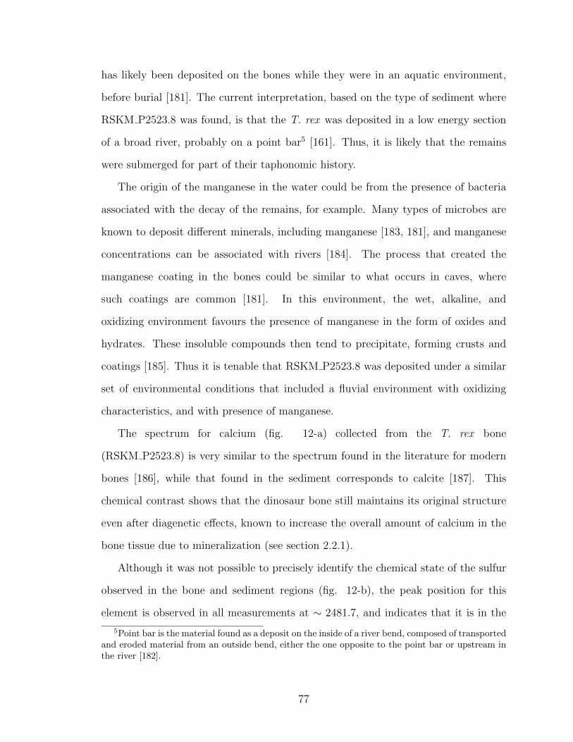
has likely been deposited on the bones while they were in an aquatic environment,
before burial [181]. The current interpretation, based on the type of sediment where
RSKM P2523.8 was found, is that the T. rex was deposited in a low energy section
of a broad river, probably on a point bar5 [161]. Thus, it is likely that the remains
were submerged for part of their taphonomic history.
The origin of the manganese in the water could be from the presence of bacteria
associated with the decay of the remains, for example. Many types of microbes are
known to deposit different minerals, including manganese [183, 181], and manganese
concentrations can be associated with rivers [184]. The process that created the
manganese coating in the bones could be similar to what occurs in caves, where
such coatings are common [181]. In this environment, the wet, alkaline, and
oxidizing environment favours the presence of manganese in the form of oxides and
hydrates. These insoluble compounds then tend to precipitate, forming crusts and
coatings [185]. Thus it is tenable that RSKM P2523.8 was deposited under a similar
set of environmental conditions that included a fluvial environment with oxidizing
characteristics, and with presence of manganese.
The spectrum for calcium (fig. 12-a) collected from the T. rex bone
(RSKM P2523.8) is very similar to the spectrum found in the literature for modern
bones [186], while that found in the sediment corresponds to calcite [187]. This
chemical contrast shows that the dinosaur bone still maintains its original structure
even after diagenetic effects, known to increase the overall amount of calcium in the
bone tissue due to mineralization (see section 2.2.1).
Although it was not possible to precisely identify the chemical state of the sulfur
observed in the bone and sediment regions (fig. 12-b), the peak position for this
element is observed in all measurements at ∼ 2481.7, and indicates that it is in the
5Point bar is the material found as a deposit on the inside of a river bend, composed of transportedand eroded material from an outside bend, either the one opposite to the point bar or upstream inthe river [182].
77

form of sulfate [188].
The data collected for iron also show different iron states for all measured
regions (fig. 12-c). For iron, I was not able to identify the specific compounds
present. However, the most interesting aspect of the iron observations is related to
the transition region between bone and sediment. Here, the chemical state of iron
cannot be explained as a linear combination of the states observed in the bone and
sediment region, which seems to be the case for the other elements analyzed. This
different state in the transition zone could potentially be related to the manganese
layer observed in the region.
Also, the position of the pre-edge peaks in the iron XANES measurements (see
arrow in fig. 12-c) can be related to iron’s oxidation state in the compound. In
the case presented, the pre-edge centroid for the transition was measured (using a
fitting method, see fig. 14) to be at 7114.18 ± 0.17eV, indicating the presence of
Fe(III) [189]. The presence of Fe(III) has been associated with the preservation of
dinosaur remains, including soft tissues in previous studies (see [7]). In [7], it was
determined the iron was in the form of goethite, which could also be the case for
this specimen. For the other measurements in the bone and sediment, the centroid
was found at 7115.24± 0.15eV (fig. 13) and 7114.94± 0.15eV (fig. 15), respectively,
which does not provide information on the oxidation state of the iron, but suggests
a transition between the 1s level to 3d level6. This transition is also observed in
corroded archaeological ferrous objects containing chlorine (see [190] for example).
The chemical state of strontium shown in fig. 12-d could not be measured with
the same accuracy achieved for the other elements, resulting in a noisier spectrum.
Due to this fact, I was unable to accurately identify the chemical states of strontium
in bone and sediment. However, it seems like this chemical state is different between
these two regions as it is suggested based on the position of the edge, which is located
61s and 3d levels refer to the atomic orbitals, i.e., the possible energy states in an atom.
78

at slightly different positions in the bone and sediment, and that the sediment edge
peak (red arrow in the figure) seems narrower than that measured in bone tissue.
The oxidation state is probably the same in both cases, since the strontium measured
seems to be Sr2+, due to the observed edge peak located at the energy ∼ 16113 eV
[191].
4.6 Conclusions
RSKM P2523.8 still maintains intact its bone microstructure. This microstructure
can be observed both using optical microscopy and chemical mapping of bone
samples such as calcium, strontium and yttrium. The findings, presented in this
research, show a manganese coating in RSKM P2523.8 bones. The presence of this
coating in the T. rex, but not in the hadrosaur specimen studied, may be related to
the environment where the dinosaur died, since it is known from sediment analysis
that RSKM P2523.8 died in an aquatic environment, by a river. No other previous
mentions of a manganese coating were found for North American dinosaur remains,
although the general preservation pattern of RSKM P2523.8 has been suggested to
be similar to that of other Tyrannosaurus discoveries [140].
The series of observations developed also points to few modifications of the
skeleton as a result of diagenetic effects, including: 1) an increase in the amount of
strontium and iron in relation to the amount of calcium; and 2) the appearance of
yttrium, which is not found in bones of extant animals. The elemental distributions
of strontium (and yttrium, in some cases) show a significant concentration of this
element restricted to the walls of canals within the bone. These canals are usually
filled with minerals that infiltrate the bone during fossilization and diagenesis, and
are also a source for the exchange of materials with the bone tissue.
The XANES measurements indicate that there are clear differences between
materials in bones and associated sediments. This includes the fact that the calcium
79
present in the bone region appears chemically similar to the calcium in extant
bones, while it appears as calcite in the surrounding sediment.
Together with the other results discussed above, it is clear that these T. rex bones
have more original characteristics preserved than just their general morphology. They
also present preserved microstructures and chemical aspects that have been maintened
in great details, even after millions of years of burial.
80

5 Non-destructive chemical analysis of insect
inclusions in amber
5.1 Abstract
Amber is polymerized tree resin, and can be responsible for exceptional preservation
of trapped biota. It provides protection to insect remains from predation, microbial
decay and other environmental factors, favouring their preservation. Previous
research has shown detailed morphological preservation in insect inclusions,
including soft tissues. However, the chemical analysis of these specimens usually
results in their destruction, because the amber must be cracked to remove the insect
material for testing. The aim of this study is to apply synchrotron radiation
techniques to the non-destructive chemical analysis of insect inclusions in amber;
specifically, ants (Hymenoptera: Formicidae) in Baltic amber. The results obtained
for iron (section 5.5.1) show that X-ray fluorescence can be used to chemically map
the insects while still encased within amber, providing information on the presence
of different elements, such as iron and calcium (as long as concentrations are high
enough) as well as their distribution in the specimen. The success of the
measurements is dependent on the quality of preservation of the insects, and on
preparing the samples to guarantee a consistent and thin amber layer on top of the
inclusion. The combination of chemical mapping with X-ray micro-CT (as imaging
technique), and XANES to define the chemical state of the iron found in the
specimens (section 5.5.2) resulted in a more complete study of the preservation of
these ants, showing the association between the chemical distribution of elements
and preserved tissues within the insects’ bodies. As a result, I was able to determine
that all ants studied had soft tissues preserved and that they were associated with
the presence of iron or calcium in the corresponding chemical maps. Specifically the
iron species was identifed as Fe(III) using XANES, which has previously been
81

associated with the preservation of soft tissues in fossils. A version of this paper has
been published in [192].
5.2 Introduction
The main subjects of the research presented in this chapter are three specimens of ant
inclusions in Baltic amber. Baltic amber is the name given to the amber found in a
series of deposits in Europe, mostly in the coastal region close to the Baltic Sea [193].
It is believed to have originated in a European forest that covered a large continental
area. The resin producers have not yet been completely established: although some
results suggest the producer to be a pine relative, the chemical analysis of the resin
in the amber suggests a composition much closer to that of the resin from extant
Araucariaceae or Sciadopityaceae [193, 194]. In chemical terms, Baltic amber can be
characterized by a specific feature present in infrared spectra known as the “Baltic
Shoulder”. It appears as an absorption band between 1250 and 1175 cm-1 that is not
seen in any other type of European amber [193].
The amber deposits found today are a result of many transport events. The first
transport is believed to have taken place shortly after the resin production occurred
near seasonal rivers. This transport took part of the material produced in the forest
to depositional environments that offered protection against weathering [193]. The
dating of these secondary deposits gives a minimum of 50 million years of age to these
amber deposits [193, 195]. Another large transport event occurred in the Pleistocene,
around 2 million years ago, when glacial movements transported rocks and debris
(including amber pieces) into Northern Europe [193, 195].
Baltic amber, though predominantly yellow, can be found in 200 different colour
varieties. The yellow tone ranges from a light yellow to orange and dark yellow and
even brown [195]. The animal inclusions found within are mostly from the Arthropoda
(98% of inclusions), but other invertebrates, including Protozoa, Nematoda, Annelida
82

and Mollusca can also be found (0.5%), as well as vertebrate-related material (0.5%)
such as bird feathers, mammal hairs and small reptiles. Plants are mostly found
as “stellate hairs”, which are predominantly branched epidermal trichomes that are
associated with oak tree leaves and flower buds [195]. Trichomes can be found in
more than half of all inclusion-bearing specimens, although occasionally other plant
types of fragments can also be found. The presence of microorganisms and fungi in
Baltic amber is rare [195].
Insects are arthropods characterized by the presence of three major tagmata:
head, thorax and abdomen, with the thorax bearing six legs [81]. The head is
responsible for sensory input, feeding and neural integration, but it is mostly
composed of muscle tissue, leaving little space for the brain, which is usually small.
The thorax is used primarily for locomotion and is dominated by muscle tissue,
while the abdomen is responsible for digestion, mating, and also some sensory input
[81]. As in all arthropods, insects are encased in a chitinized cuticle that provides
protection and support for their bodies. The exoskeleton helps in locomotion and
communication, prevents water loss, provides a site for waste deposition and offers
protection [81]. With this basic body structure, there are no calcified hard parts in
insects, and the plates (sclerites) that make up each body region are bound by
flexible membranes, so they scatter or decay in many preservational settings (e.g.,
[197]). Amber is one of the few means of detailed preservation for insects, but the
roles of differing amber chemistries, and the sequence of taphonomic events needed
to preserve details such as soft tissues are still being investigated [80, 198, 199].
This debate is relevant to the current study, because insects have an open
respiratory system, and it is unclear whether soft tissues are more likely to preserve
when resin is drawn into the body cavity [199].
The ants belong to the order Hymenoptera together with bees and wasps. This
order is characterized by the presence of mandibulate mouthparts and a generalized
83

ovipositor that can be used to inject eggs in spaces otherwise inaccessible, or in hosts.
Within this order, ants belong to the Aculeata, a group with a well-developed ‘waist’,
in which the ovipositor was modified to become a stinger. The family Formicidae is
thought to have had its origin at approximately 120 million years ago [81]. Based
upon the abundance and diversity of inclusions preserved in amber, formicids are only
thought to have become a dominant group approximately 70 million years ago. While
the focus of the research presented herein is in the Baltic amber specimens, some of
the insect inclusions used for comparison specimens in this chapter are from North
Carolina amber. This deposit is approximately 83.6 to 72.1 million years old, and
it has been recently reviewed [196]. Although Cretaceous ants with the same degree
of preservation as the Baltic amber specimens were not available for preparation
and analysis as part of this study, comparisons to North Carolina amber specimens
provided an opportunity to test whether the same preservational features were present
in a much older amber deposit.
Ants are relatively rare as inclusions in Cretaceous amber, and usually belong to
the exclusively Cretaceous subfamily Sphecomyrminae [200]. Recent work on Burmese
Late Cretaceous amber has demonstrated that members of this extinct subfamily are
more abundant and have a more extensive social structure than once thought, but that
ants do not occur in the same diversity and abundance that is characteristic of amber
deposits in the Eocene and Miocene [201]. The subfamilies that characterize modern
ecosystems only appear to have gained ecological dominance by the time that Eocene
Baltic amber was produced, and they figure more prominently in Miocene Dominican
amber [202]. The genera analyzed in the present study are Ctenobethylus Brues
(RSKM P3001.16 and RSKM P3000.17) and Nylanderia Emery (RSKM P3000.15).
The former genus belongs to the subfamily Dolichoderinae and is known exclusively
from Baltic amber, while the latter genus belongs to Formicinae and has modern
representatives [203]. Comparisons were also made to significantly older specimens
84
with poorer preservation, from Late Cretaceous North Carolina amber (SEMC NC
272-276; Sphecomyrminae: Baikuris Dlussky), and modern formicids.
The focal point for previous soft tissue studies in amber has been larger inclusions
of Hymenoptera and Diptera (e.g., [204]; [104]), and these early studies have utilized
destructive sampling to analyze tissues preserved within the body cavity. In fact,
most chemical analysis of amber inclusions is destructive (i.e., the insect inclusion
is deliberately damaged so that measurements can be taken). More recently, non-
destructive techniques have been employed more often in amber studies. The most
commonly used to characterize amber inclusion compositions has been Confocal Laser
Scanning Microscopy (CLSM), which has provided successful results for fungi and
plant trichomes (e.g., [205]). Because this technique measures the autofluorescence
of the preserved tissues, it is not suitable to be applied to a wide range of inclusions,
due to its dependence on their autofluorescence properties [205]. Moreover, the types
of molecules studied are limited by the wavelengths (and, therefore, energies) of the
laser light available and, in some deposits, the amber also autofluoresces, causing a
masking effect on the results (e.g., [206]).
Synchrotron light has been used more commonly as a tool to obtain
morphological information on inclusions, using techniques such as synchrotron
radiation X-ray microtomography (SR X-ray μCT) as can be seen in [207, 208], for
example. This technique is especially useful when studying inclusion within opaque
amber, where more conventional techniques (such as optical microscopy) cannot be
applied [209]. French Cretaceous amber specimens were the first to be studied using
synchrotron μCT [207, 210], but subsequently many others have been imaged [209].
Among the results obtained are larval stages for several groups of insects [209]; and
anatomical details of the oldest representative of the beetle family Monotomidae
[208]. Other examples of anatomical studies of insect inclusions using synchrotron
μCT can be found in [211, 212, 213]. The only taphonomic studies to make use of
85

synchrotron observations are those of McCoy et al. [198, 199], where the extent of
soft tissue preservation visible in CT data is tied to resin type. McCoy also used
bubbles within the body cavity are to estimate extent of decay.
As a tool for obtaining chemical information from fossils, synchrotron light has
usually been applied to larger specimens in sedimentary rocks, such as the remains of
avian and non-avian theropods and reptiles (e.g., [152, 215]). The primary technique
for these analyses has been Synchrotron Rapid Scanning X-ray Fluorescence (SRS-
XRF), which has been reviewed in [153]. This technique has been used to study the
extinct bird Archaeopteryx. The phosphorus distribution, for example, was used to
identify teeth that were not apparent in measurements using visible light, and also
showed that its feathers were preserved structures instead of impressions [153, 152].
The chemical information from smaller fossils is usually obtained using Scanning
Electron Microscopy (SEM) and Energy Dispersive Spectrometry (EDS) (e.g., [216,
217]), but these forms of analysis require exposures that are seldom available in amber
without cracking specimens open.
This study investigates the application of synchrotron X-ray fluorescence as a non-
destructive technique to obtain chemical information of insect inclusions in amber.
The first goal of this research was to understand the potential and limitations of the
use of this technique for different amber specimens. In the second portion of this
study XRF is used in combination with synchrotron μCT and XANES to study ants
in Baltic amber, and how their chemistry is related to their preserved tissues.
5.3 Material and methods
5.3.1 Specimens and preparation
Four ant (Hymenoptera: Formicidae) inclusions in amber and two modern ants were
selected for this research. The amber specimens (listed in table 1) were embedded in
mineralogical-grade epoxy (Epo-Tek 301) and cut with a water-cooled lapidary saw.
86

The cuts were made in order to reduce the width of the amber layer on top of the
insect inclusion as much as possible, which, in practical terms, was on the order of 1 to
2 mm thick. The cut specimens were polished with lapidary wheels and wet sanding
baths to further reduce the thickness of the amber layer. This procedure follows [218]
for the preparation of fragile amber pieces and it is a common preparation procedure
for obtaining proper anatomical views, and studying amber specimens using light
microscopy (e.g., [219, 220]). The final samples (amber blocks) were approximately
2 mm thick in total, including the size of the inclusion. The overlying amber layer
in these samples varied between tens to hundreds of micrometers, depending on the
specimen and limb orientation. Since polishing to the point of exposing any part of
the insect, including appendages, would result in damaging the inclusion, the polished
surfaces toward which the appendages were oriented ended up thicker than the others
in relation to the insect’s main body. Once this process was finished, the samples were
cleaned with isopropanol to remove surface contaminants from handling.
Type Number of specimens Specimen names
Modern ants 2 RSKM P3314.2, RSKMP3314.1
Baltic amber 3 RSKM P3000.15, RSKMP3000.16, RSKM P3000.17
North Carolina amber 1 SEMC NC 272-276
Table 1: List of specimens analyzed.
Samples of modern ant specimens were also prepared in order to compare with the
results obtained from fossils, and provide a control for some of the materials being
examined. In this case, two ants were inserted into the same epoxy resin used in
preparing the amber specimens. One of the ants was added to the resin once dead
(RSKM P3314.2), while the other was added while still alive (RSKM P3314.1), in
order to observe if resin infilling the body cavity due to movement would have an
effect on the results, and if observable differences in the fossil specimens could be
87
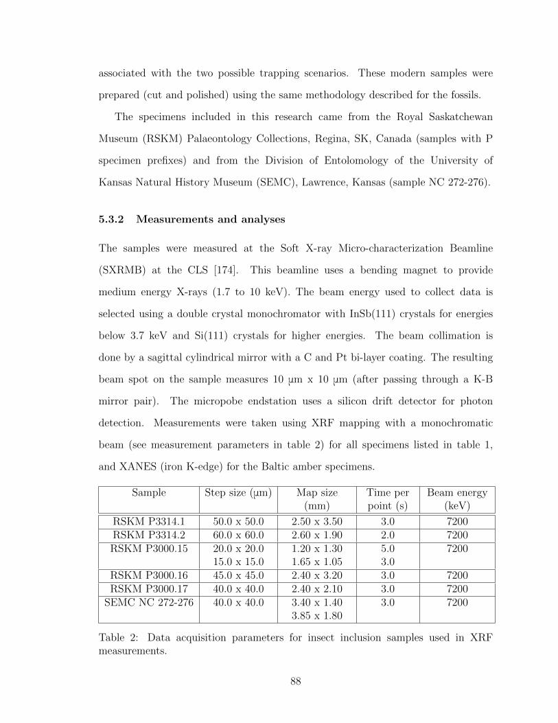
associated with the two possible trapping scenarios. These modern samples were
prepared (cut and polished) using the same methodology described for the fossils.
The specimens included in this research came from the Royal Saskatchewan
Museum (RSKM) Palaeontology Collections, Regina, SK, Canada (samples with P
specimen prefixes) and from the Division of Entolomology of the University of
Kansas Natural History Museum (SEMC), Lawrence, Kansas (sample NC 272-276).
5.3.2 Measurements and analyses
The samples were measured at the Soft X-ray Micro-characterization Beamline
(SXRMB) at the CLS [174]. This beamline uses a bending magnet to provide
medium energy X-rays (1.7 to 10 keV). The beam energy used to collect data is
selected using a double crystal monochromator with InSb(111) crystals for energies
below 3.7 keV and Si(111) crystals for higher energies. The beam collimation is
done by a sagittal cylindrical mirror with a C and Pt bi-layer coating. The resulting
beam spot on the sample measures 10 μm x 10 μm (after passing through a K-B
mirror pair). The micropobe endstation uses a silicon drift detector for photon
detection. Measurements were taken using XRF mapping with a monochromatic
beam (see measurement parameters in table 2) for all specimens listed in table 1,
and XANES (iron K-edge) for the Baltic amber specimens.
Sample Step size (μm) Map size(mm)
Time perpoint (s)
Beam energy(keV)
RSKM P3314.1 50.0 x 50.0 2.50 x 3.50 3.0 7200RSKM P3314.2 60.0 x 60.0 2.60 x 1.90 2.0 7200RSKM P3000.15 20.0 x 20.0
15.0 x 15.01.20 x 1.301.65 x 1.05
5.03.0
7200
RSKM P3000.16 45.0 x 45.0 2.40 x 3.20 3.0 7200RSKM P3000.17 40.0 x 40.0 2.40 x 2.10 3.0 7200
SEMC NC 272-276 40.0 x 40.0 3.40 x 1.403.85 x 1.80
3.0 7200
Table 2: Data acquisition parameters for insect inclusion samples used in XRFmeasurements.
88
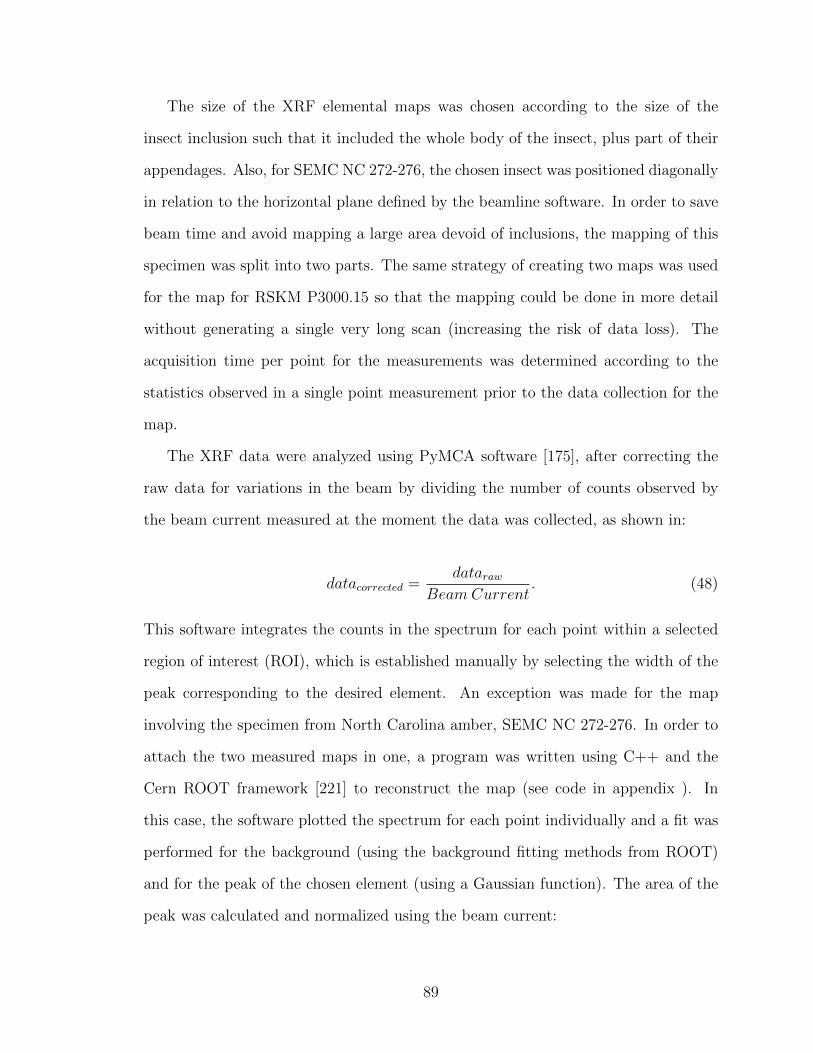
The size of the XRF elemental maps was chosen according to the size of the
insect inclusion such that it included the whole body of the insect, plus part of their
appendages. Also, for SEMC NC 272-276, the chosen insect was positioned diagonally
in relation to the horizontal plane defined by the beamline software. In order to save
beam time and avoid mapping a large area devoid of inclusions, the mapping of this
specimen was split into two parts. The same strategy of creating two maps was used
for the map for RSKM P3000.15 so that the mapping could be done in more detail
without generating a single very long scan (increasing the risk of data loss). The
acquisition time per point for the measurements was determined according to the
statistics observed in a single point measurement prior to the data collection for the
map.
The XRF data were analyzed using PyMCA software [175], after correcting the
raw data for variations in the beam by dividing the number of counts observed by
the beam current measured at the moment the data was collected, as shown in:
datacorrected =dataraw
Beam Current. (48)
This software integrates the counts in the spectrum for each point within a selected
region of interest (ROI), which is established manually by selecting the width of the
peak corresponding to the desired element. An exception was made for the map
involving the specimen from North Carolina amber, SEMC NC 272-276. In order to
attach the two measured maps in one, a program was written using C++ and the
Cern ROOT framework [221] to reconstruct the map (see code in appendix ). In
this case, the software plotted the spectrum for each point individually and a fit was
performed for the background (using the background fitting methods from ROOT)
and for the peak of the chosen element (using a Gaussian function). The area of the
peak was calculated and normalized using the beam current:
89

Areaplotted =Areapeak − Areabackground
Beam Current(49)
The resulting value was used for each pixel in the map.
The elemental maps of the specimens from Baltic amber were combined with
their respective tomography images in order to match the features observed using
the two techniques. The tomography measurements were taken at the BioMedical
and Imaging Therapy (BMIT) Insertion Device (ID) beamline at the CLS [222] by
Ryan C. McKellar. The images were reconstructed by Gavin King using the AMIRA
software pratform (ver 6.3) and the Z-Brush software (ver. 4R7 P3) (more details can
be found in [223]). Interpretive drawings of tissues within the tomography data sets
were created using AMIRA translucent volume renderings, and then tracing tissue
outlines on still images using Adobe Photoshop (ver. CS5) and Autodesk Sketchbook
Pro (ver. 6.0.1) software. The final images were combined using the software ImageJ
[224] by creating an overlay of the elemental maps (at 80% transparency) on the
tomography images. The elemental maps were adjusted in size and angle to match
the tomography image.
The XANES data were analyzed using Athena software [128]. The pre-edge region
was fitted using an error function (equation 46) to describe the sharp rise of the edge,
combined with one or two Gaussian functions to describe the pre-edge structures in
the spectrum. The choice of these functions was based on a set that resulted the
lowest χ2/NDF for the fit, with the error function and arctan describing the K-edge
and with the Gaussian and pseudo-voigt options for the peaks, which are the curves
commonly used for such fittings in previous experiments [189].
90

5.4 Results
5.4.1 XRF applied to insect inclusions
The elemental maps produced using XRF for the modern ants are presented in fig.
16 for RSKM P3314.1, and in fig. 17 for RSKM P3314.2. Only the elements showing
an informative distribution were included in the plots presented. Additional elements
in the same energy range were also analyzed, but their maps only resulted in noise
with no discernible patterns.
Figure 16: Elemental maps of Ca, Cl, Fe and K for RSKM P3314.1 compared to itsmicroscope image. (Original in colour)
Figure 17: Elemental maps of Ca, Cl, Fe and K for RSKM P3314.2. (Original incolour)
91

Fig. 16 shows that the amount of calcium, iron and potassium seem to be higher
in the region of the insect’s head. The distribution of chlorine is the negative of the
distributions of the other elements (i.e., it shows a high amount everywhere but on
the region of the insect’s head). Fig. 17 exhibits a similar pattern, but in this case
calcium and potassium appear in larger quantities in the abdomen of the insect, while
iron appears in the whole body. Again chlorine appears everywhere but in the regions
where the other elements are abundant.
Three specimens of ant inclusions in Baltic amber were mapped using XRF: RSKM
P3000.15, RSKM P3000.16 and RSKM P3000.17 (figs. 18, 19 and 20, respectively).
Iron was the only detectable common element present with a distribution correlated
to the inclusion for all specimens studied (including also modern specimens and the
Cretaceous North Carolina amber). This element has also been linked to soft tissue
preservation in sedimentary settings [7]. Thus, it was the element chosen as the focal
point for the study on the applicability of this technique.
92
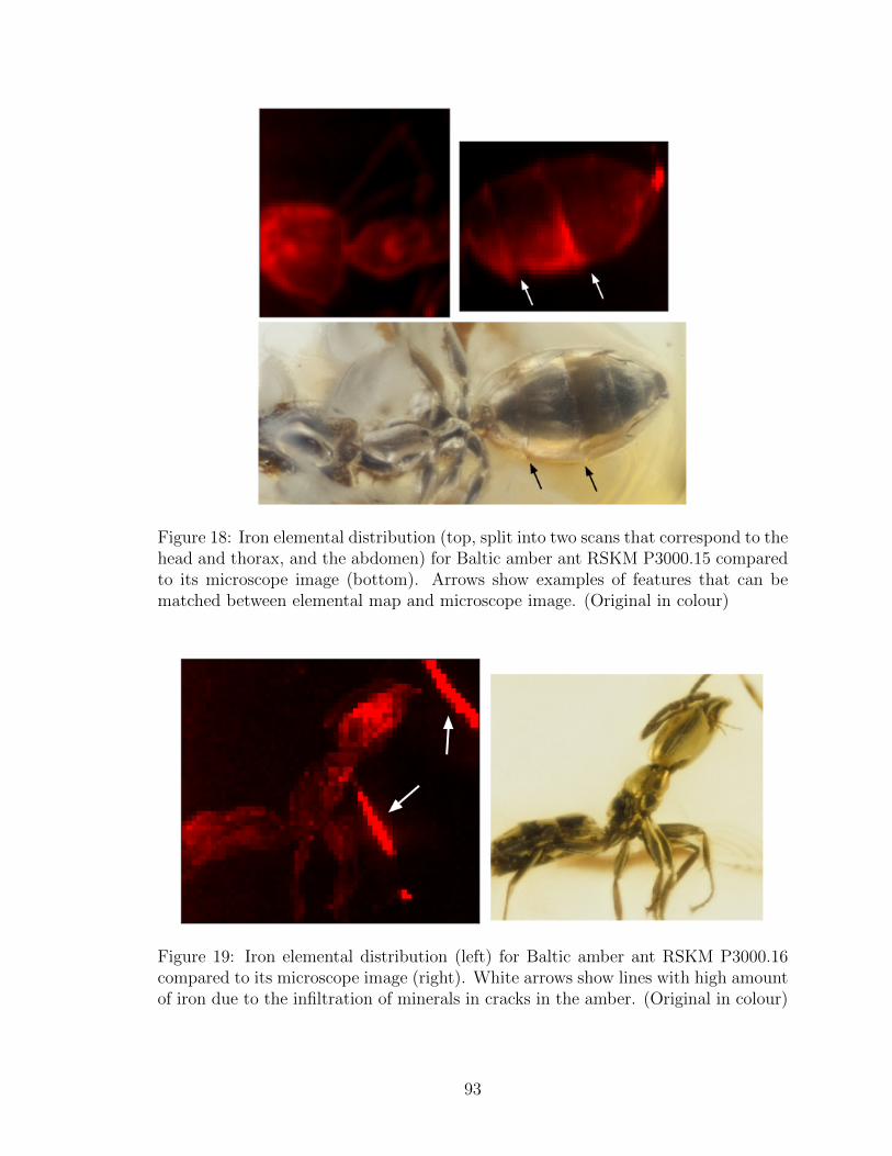
Figure 18: Iron elemental distribution (top, split into two scans that correspond to thehead and thorax, and the abdomen) for Baltic amber ant RSKM P3000.15 comparedto its microscope image (bottom). Arrows show examples of features that can bematched between elemental map and microscope image. (Original in colour)
Figure 19: Iron elemental distribution (left) for Baltic amber ant RSKM P3000.16compared to its microscope image (right). White arrows show lines with high amountof iron due to the infiltration of minerals in cracks in the amber. (Original in colour)
93

.
Figure 20: Iron elemental distribution (left) for Baltic amber ant RSKM P3000.17compared to its microscope image (right). (Original in colour)
All three specimens from Baltic amber exhibit iron distribution following the
region where the insect is located, with the highest iron levels in the region of their
heads and thoracic muscles. Some features of the distribution seem to match with
features in the microscope images, corresponding to the boundaries of sclerites and
following the outlines of the exoskeleton, such as the joints in the abdomen of
RSKM P3000.15 in fig. 18. Other characteristics of the distribution do not
correspond to any feature visible in the external images. Fig. 19 also shows lines
with large amounts of iron (marked by arrows), which are the result of infiltration of
minerals in cracks in the amber.
The specimen from North Carolina amber SEMC NC 272-276 contains five partial
ant inclusions, of which two were mapped (fig. 21). The area to be mapped was
selected based on previous results obtained at the Dr. David Cooper’s Lab (University
of Saskatchewan)7 using preliminary scan data obtained from X-rays imaging in a
benchtop μCT scanner.
7Cooper Lab: 3D30.3 Health Sciences, 107 Wiggins Rd, Saskatoon, SK S7N 5E5
94

Figure 21: Iron elemental map (left) for North Carolina amber SEMC NC 272-276compared to its microscope image (right). In the elemental map the scale goes fromblue to red, representing lower to higher concentrations of iron, respectively. Whiteareas were not mapped. (Original in colour)
The iron distribution shown in fig. 21 also follows the shape of the insect inclusion,
although not as well as the previous specimens. The contour of the ant in the right-
hand side is clearly visible in green in the map, showing it presents more iron than
the surrounding amber. The insect on the left side is not as clearly represented in
the map as the one on the right, and preservation of the cuticle in this specimen
is sporadic. The insect’s body shows elevated levels of iron in comparison to the
surrounding material. However, the contours are not as clear, and iron is also present
in the regions surrounding the insect.
5.4.2 Preservation of ant inclusions in Baltic amber
It is useful to combine the XRF results with a 3D imaging technique, so that it is
possible to match the chemical distribution to physical structures identified in the
inclusion at a finer level of detail. In this section, elemental maps for Baltic amber
ants, measured using XRF mapping, are combined with results from synchrotron X-
ray micro-CT results obtained from the same insects at the Bio-Medical Imaging
and Therapy Facility (BMIT) beamline at the CLS. The goal of this data
95
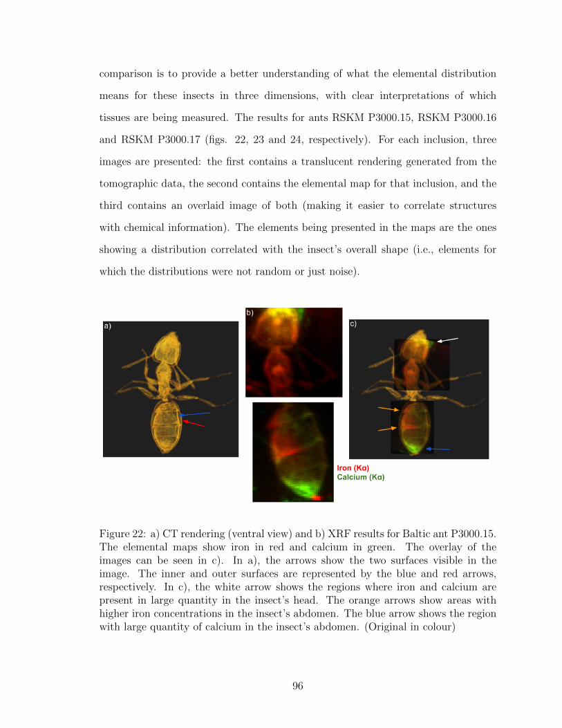
comparison is to provide a better understanding of what the elemental distribution
means for these insects in three dimensions, with clear interpretations of which
tissues are being measured. The results for ants RSKM P3000.15, RSKM P3000.16
and RSKM P3000.17 (figs. 22, 23 and 24, respectively). For each inclusion, three
images are presented: the first contains a translucent rendering generated from the
tomographic data, the second contains the elemental map for that inclusion, and the
third contains an overlaid image of both (making it easier to correlate structures
with chemical information). The elements being presented in the maps are the ones
showing a distribution correlated with the insect’s overall shape (i.e., elements for
which the distributions were not random or just noise).
Figure 22: a) CT rendering (ventral view) and b) XRF results for Baltic ant P3000.15.The elemental maps show iron in red and calcium in green. The overlay of theimages can be seen in c). In a), the arrows show the two surfaces visible in theimage. The inner and outer surfaces are represented by the blue and red arrows,respectively. In c), the white arrow shows the regions where iron and calcium arepresent in large quantity in the insect’s head. The orange arrows show areas withhigher iron concentrations in the insect’s abdomen. The blue arrow shows the regionwith large quantity of calcium in the insect’s abdomen. (Original in colour)
96
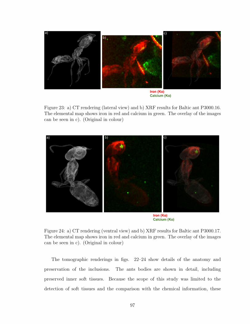
Figure 23: a) CT rendering (lateral view) and b) XRF results for Baltic ant P3000.16.The elemental map shows iron in red and calcium in green. The overlay of the imagescan be seen in c). (Original in colour)
Figure 24: a) CT rendering (ventral view) and b) XRF results for Baltic ant P3000.17.The elemental map shows iron in red and calcium in green. The overlay of the imagescan be seen in c). (Original in colour)
The tomographic renderings in figs. 22–24 show details of the anatomy and
preservation of the inclusions. The ants bodies are shown in detail, including
preserved inner soft tissues. Because the scope of this study was limited to the
detection of soft tissues and the comparison with the chemical information, these
97

structures were not characterized in detail. However, as an example, fig. 25 shows in
more detail the head of RSKM P3000.15 and the corresponding diagram for the
preserved tissues made by Ryan McKellar. In this image, it is possible to see the
preserved cuticle reinforcements (in blue, the tentorium), and traces of what could
be either the brain or digestive glands (in white). The pink area in the right side of
25-b likely represents preserved mandibular muscles. The tomographic renderings
also show two surfaces for all insects (marked with arrows in fig. 22-a, as an
example), where the external impression of the exoskeleton is recorded in the
amber, and the shrivelled remains of the exoskeleton. This means that several parts
of the insect are no longer in contact with the amber surface.
Figure 25: a) CT rendering of the head of Baltic amber ant RSKM P3000.15 (dorsalview) and b) the diagram of the preserved tissues observed in the rendering. In b), thecuticle reinforcements of the tentorium are represented in blue, mandibular musclesin pink, and traces of either brain or digestive glands are in white.
The elemental map for RSKM P3000.15 (fig. 22-b) shows iron and calcium
distributed along the ant’s body. Iron is more concentrated in the insect’s head,
middle of thorax, and parts of the abdomen (mostly in the lines in the cuticle, but
98

at higher concentrations within the areas that contains shrivelled tissues inside the
abdomen, and a bubble of purge fluid that has escaped the posterior end). The
same patterns are observed for RSKM P3000.16 and RSKM P3000.17, except for
the abdomen of the latter, which appears to have low amounts of all elements. This
apparent low concentration is likely influenced by the angle the insect was
positioned within the amber (i.e., the abdomen was farther from the amber surface).
The calcium distribution in fig. 22-b seems to be more concentrated in the head and
abdomen of the ant. As was the case for iron, calcium is present in larger quantities
along the margins of the abdominal sclerites, but it is also found in its much higher
concentrations within the posterior region. The other specimens do not present such
a clear calcium distribution as RSKM P3000.15, but they also show this element is
present. RSKM P3000.16 (fig. 23-b) shows high concentractions of calcium in the
region of amber outside of the inclusion, and this appears to trace decay products
trapped on a flow line in the amber. The structures present in the elemental maps
are shown to match structures present in the tomographic renderings in the overlay
images (figs. 22-c, 23-c, and 24-c).
Although low, the statistics collected in the SXRMB beamline were sufficient to
provide significant iron K-edge XANES measurements for the insects’ heads. Areas
of high iron concentration were investigated for all insects in these measurements.
The results obtained for the amber insects, as well as for the modern ant depicted
in fig. 16, can be seen in fig. 26. The spectra in fig. 26 were normalized following
the Athena software package standard parameters. The amounts of calcium found in
these samples were not enough to obtain the corresponding spectra for this material.
99

Figure 26: Iron K-edge XANES results for measurements taken from the head capsulesof Baltic amber ants compared to a modern ant (RSKM P3314.1). The spectra werenormalized and are presented a) together and b) stacked with 0.2 interval betweendifferent spectra. RSKM P3000.15 is shown in blue, RSKM P3000.16 in purple,RSKM P3000.17 in green, and RSKM P3314.1 in red. The arrows mark the positionof the edge. (Original in colour)
These measurements (fig. 26) show similar spectra for all samples, with some
differences. The position of the K-edge (see arrows) seems to be constant for all
samples. However, the pre-edge region seems to match for all the specimens except
RSKM P3000.15. These pre-edge peaks were fitted using an arctan function to
describe the edge and Gaussian curves for the pre-edge peaks (as many as necessary
to describe the data) and the results can be seen in figs. 27, 28, 29 and 30.
Figure 27: Iron pre-edge fit for Baltic ant specimen RSKM P3000.15, showing a)fitting line and residual and b) a magnified image of the pre-edge region and theindividual functions used in the fitting. (Original in colour)
100
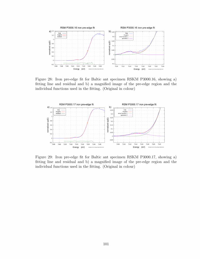
Figure 28: Iron pre-edge fit for Baltic ant specimen RSKM P3000.16, showing a)fitting line and residual and b) a magnified image of the pre-edge region and theindividual functions used in the fitting. (Original in colour)
Figure 29: Iron pre-edge fit for Baltic ant specimen RSKM P3000.17, showing a)fitting line and residual and b) a magnified image of the pre-edge region and theindividual functions used in the fitting. (Original in colour)
101

Figure 30: Iron pre-edge fit for Baltic ant RSKM P3314.1, showing a) fitting line andresidual and b) a magnified image of the pre-edge region and the individual functionsused in the fitting. (Original in colour)
The pre-edge Gaussian peaks were found at 7114 eV for all samples (the exact
values for RSKM P3000.15, RSKM P3000.16, RSKM P3000.17 and RSKM P3314.1
are 7114.00 eV, 7114.04 eV, 7114.77 eV and 7114.26 eV, respectively). Specimen
RSKM P3000.15 needed a second Gaussian to fit the pre-edge, resulting in another
peak at 7119.70 eV.
5.5 Discussion
5.5.1 XRF applied to insect inclusions
Modern ants Single point measurements8 obtained from the epoxy resin areas of
the samples (without insect contents) showed that out of the elements in the energy
range measured, only chlorine was present. This can also be observed in the elemental
map for this element, where Cl shows a higher concentration in all points measured
except for the ones on top of the insect (figs. 16 and 17). Within these regions, the
resin layer is thinner due to the presence of the inclusion. Thus, chlorine cannot be
studied using this characterization technique if this type of epoxy resin is used as
8Single point measurements are taken at a single position in the sample. The data for thesemeasurements could not be saved, because the software used at the SXRMB beamline at the timeof the experiment did not offer this option.
102
a mountant or amber support. The result of this measurement also shows that the
composition of the resin should not interfere with the measurements for iron discussed
later in this section, but could be used to investigate possible cracks in the amber. If
such cracks are present in the sample, the resin will infiltrate and these will appear
as regions with high chlorine concentration on the chemical maps.
Although the epoxy resin composition does not affect the results of the
measurements, the same cannot be said about its thickness. The thickness of resin
layer (or amber, for it has a similar effect) causes attenuation of the signal both
when the X-ray beam is traveling through the material before reaching the inclusion,
and in the fluorescence photons that are travelling in the direction of the detector.
As a result, areas where the resin or amber layer is thicker will show an apparent
lower concentration of the element being measured than other parts of the insect,
despite the same real concentration in the specimen itself. Thus, geometric aspects
of the insect, such as its shape and angle in relation to the measured surface, may
introduce differences in the measured signal. Although inevitable, the attenuation
effects discussed can be minimized during sample preparation by positioning the
insect as close as possible to a parallel direction relative to the measured surface.
Apart from geometric effects caused by differences in the positioning of the two
ant specimens, no significant differences were observed between the ant that was
embedded in the resin alive compared to the one that was dead. The measured
distributions include the same elements for both samples. Also, comparable chemical
patterns detected in both modern ants show that there are no detectable differences
in measured elemental composition, based on the way the insect died and interacted
with the surrounding resin.
Baltic amber The presence of iron as the only detectable element may be the result
of the attenuation effects imposed by the amber layer between insect and detector.
103
Since elements with lower atomic numbers predominantly emit fluorescence photons
with lower energy and the penetration depth of light in a material depends on its
energy, it is logical that measurements involving elements with a low atomic number
will be subject to larger attenuation effects. Thus, the techniques employed here are
not suitable to ascertain if lighter elements are absent in these specimens, or if the lack
of signal is a result of light attenuation in the sample, or a combination of both factors
(e.g., if the insect had initially a very low concentration of an element that cannot
be measured due to attenuation effects). This question could possibly be answered
after careful calculations involving the properties of amber and the thickness of the
layer present. However, such values are difficult to obtain due to the irregular surface
of the insect inclusion. Elements with higher atomic numbers than iron could not be
detected due to the achievable beam energy range at the SXRMB beamline, which
sits outside the energy region needed to excite the atoms of these elements.
Light attenuation effects are also present in the iron measurements. This
attenuation effect could lead to differences in the measured concentrations that are
independent of the actual composition of the inclusion. Consequently, the maps
present the locations where iron is found in the insect, but differences in the
attenuation caused by variations in the thickness of the amber overlying the insect
could lead to apparent variations in the relative concentration of iron within the
inclusion. In order to obtain more conclusive results, it would be useful to include
an additional three-dimensional imaging measurement. This could present visual
information on the insect’s structures and their positioning and better account for
such geometric effects (see section 5.5.2).
The qualitative interpretation of these results provides valuable distribution
information, which is not attainable through conventional characterization
techniques. Apart from the surrounding amber being shaped and prepared, it is a
non-destructive and non-invasive measurement that leaves the insect inclusion
104

intact. Iron is an element of biological relevance for virtually all organisms,
including insects [225]. It is found in significant amounts in insects while they are
still alive, but iron is also produced as a result of soft tissue decay after their death
[226]. The careful study of iron could, therefore, provide more taphonomic
information about the preservation of insect inclusions in amber. Although XRF
can be used in a quantitative fashion, it is improbable that such an approach could
be taken in the context of the specimens studied here, due to effects such as the
ones introduced by the thickness of the amber layer on the sample, insect
orientation and shape, and the chemical heterogeneity present in these specimens.
North Carolina amber It is possible to faintly see the outline of the inclusions
in the iron distribution present in the map, in fig. 21. However, its definition is not
nearly as clear as those observed in the maps of Baltic amber ants (figs. 18 to 20).
This can be explained by differences in the preservation of these insects. Baltic amber
is known for the exceptional quality of preservation of its inclusions [81], while the
North Carolina amber specimens are also much older [227] and visibly not as well
preserved, at least at the exoskeleton level. In these specimens, the exoskeleton has
become carbonized and broken up into sheets of cuticle [80], leading to a decrease in
the amount of tissue preservation and iron remaining in the specimen. Nevertheless,
some iron content seems to have been preserved within the highly altered SEMC NC
272-276 remains as can be observed from the iron distribution shown in the elemental
map. This trace of iron suggests that the technique could be successfully applied to
a wider range of inclusions, as far back in time as the Cretaceous.
SEMC NC 272-276 could not be mapped with the same quality as the specimens
discussed previously, because the amber surface on top of the insects had a round
shape that could not be cut or polished without destroying the inclusions. This
meant that the thickness of the amber layer was variable during data acquisition,
105

causing possible beam focusing issues9 that can impact the overall quality of the
measurements obtained here. The general correspondence between cuticle presence
and iron concentrations seems to match the patterns observed in younger specimens,
but a wider range of Cretaceous samples prepared for this form of analysis are required
to make detailed inferences.
5.5.2 Preservation of ant inclusions in Baltic amber
The tomographic renderings of the three Baltic amber ants show that all of them
present preserved internal tissues (see fig. 25, for detailed example), which appear to
be correlated with areas that exhibit higher concentrations of iron or calcium in the
maps. Preserved soft tissues in amber inclusions have been previously identified in
several specimens (e.g., [104, 229, 198]). For Baltic amber especifically, a summary
from 2017 showed that out of 27 specimens studied using techniques that would allow
for identification of soft tissues, 11 of them had preserved internal structures [198].
Iron is expected to be found in large quantities in insect tissues, since it is
present in their vascular system [230] and is important to their metabolism [231].
This can be observed in the images provided such as in fig. 22-c that shows iron
preserved in large quantities in the ant’s head (white arrow in fig. 22), which is
correlated with the preserved mandible muscles visible in the CT data. The same
figure also shows areas with higher iron concentrations in the insect’s thorax,
correlated with the thoracic muscles (bright area in middle of thorax in fig. 22).
Elevated concentrations in the insect’s abdomen are correlated with regions of the
cuticle and shriveled organs (orange arrows in fig. 22). The iron measured in the
insects, therefore, is almost certainly original to the insects or, perhaps, a result of a
taphonomic process responsible for the preservation of soft tissue structures (as
9If the beam is not properly focused, the beam spot in the sample becomes larger and moredispersed than what it should be. Thus, the measurements would be performed over an area largerthan expected. The practical result of this is that the resulting image loses definition and becomesmore blurry.
106

opposed to iron that has infiltrated). If iron had been introduced, it would probably
be more evenly distributed within the insects, and exhibit a clear path from an
infiltration point, instead of correlating to just the preserved remains of organs and
cuticle. In fig. 23, iron also appears in the region of amber outside of the insect in
diagonal line close to the insect’s head. This is line is most likely caused by a crack
in the amber, resulting on infiltration of minerals, which are not related to the
inclusion.
In RSKM P3000.15 (fig. 22), the calcium distribution is mainly correlated with
iron in areas where the mandible tissues appear preserved (white arrow in fig. 22)
and in the posterior portion of the ant’s abdomen where the concentration of iron is
not high (blue arrow in fig. 22). Calcium in modern insects can be found as part of
the haemolymph, and is distributed in lower concentrations within their soft tissues
[232]. Figs. 16 and 17, for example, show calcium distributed in the insect’s body.
In the mandibles in particular, insects are known to accumulate metals, such as the
iron and calcium to increase the strength and reduce wear on these structures [233].
This would explain the presence of calcium in the area where muscle tissues were
preserved. Calcium is also deposited in insects’ midguts [232], which could suggest
that the high concentration observed in the abdomen could be related to a collapsed
midgut in the insect. This is corroborated by the presence of preserved internal tissue
visible in the tomographic images that exactly match the distribution of calcium in
the area.
The calcium distribution seems to be more consistent with insect soft tissue
structures in the RSKM P3000.15 (fig. 22) than in the other specimens examined.
In the case of RSKM P3000.17 (fig. 24) the distribution could be due to the fact
that the insect is at an angle relative to the surface of the amber, with its abdomen
farther from the surface than its head. This orientation causes an attenuation effect
in the iron distribution compared to other parts of the insect, an effect that is
107

intensified for calcium due the lower energy of the photons emitted from these
atoms. Since the abdomen is where most of the Ca is located in RSKM P3000.15, I
cannot conclude from these measurements whether RSKM P3000.17 actually
possesses a comparable distribution of this element or, if I am simply unable to
measure such a distribution due to sample geometry differences. From what the
measurements show, it seems Ca in RSKM P3000.17 is a taphonomic product of the
decay and expulsion of the ant’s digestive system. In the case of RSKM P3000.16
(fig. 23), however, the calcium distribution seems to be completely outside of the
insect, as vesicles within the surrounding amber. This external distribution could
have been caused by haemolymph or decay products leaking out into the resin, or
by infiltration from surrounding minerals with carbonate content.
Another common characteristic for all analyzed Baltic amber inclusions (although
more visible in RSKM P3000.15 and RSKM P3000.17) is that two surfaces can be
seen in the tomographic renderings. The outmost surface corresponds to the original
outline of the insect, while the inner surface corresponds to the shriveled remains
of the cuticle. These two surfaces are preserved by solidification of the resin into
amber before the insect underwent dehydration and loss of volume. This feature
suggests that the insect was trapped in the resin and completely encased before it
had time to undergo significant decay, or to dehydrate due to exposure. Thus, the
taphonomic changes observed were reduced by the presence of a surrounding amber
layer, resulting in excellent preservation. In turn, the level of preservation found in
these insects is what makes it possible to obtain high quality synchrotron data —
which means that observing the inclusion withdrawn from its original outline in the
surrounding amber can be used as a way to estimate which samples are more likely
to yield better defined elemental map scans using synchrotron light. Since beam time
at synchrotron facilities is limited, this taphonomic feature can be used to reduce
wasted time with insects that will not provide clear results.
108

The iron spectra in fig. 26 show that all samples have slightly different curves,
although the position of the edge (black arrows in the figure) is maintained for all
of them. In particular, RSKM P3314.1 has an edge with a very different shape (red
spectra in the figure) compared to the other samples. Although the compounds to
which the iron belongs in each specimen could not be identified with confidence, the
iron oxidation state can be obtained based on the position of the pre-edge peak. This
peak seems to be the same for all samples (considering the noise in the measurements),
except for sample RSKM P3000.15.
The results for pre-edge energies (figs. 27-30) at around 7114 eV suggests that the
iron is in a Fe(III) state, while the peak at 7119.70 eV does not provide information on
the oxidation state of the iron [189]. It is important to notice that the iron in the fossil
ants is found in the same oxidation state as the iron in the modern ant, suggesting that
the materials measured are originally from the insects, or a slightly modified version
of this original material. Moreover, ferric iron in insects is linked to the presence of
proteins such as transferrin and ferritin [228], and, thus, the measurements presented
could be the result of preserved or partially-preserved structures that were parts of
proteins in these animals.
5.6 Conclusions
XRF mapping can be used to study insect inclusions in amber in a non-destructive
and non-invasive way. This provides not only compositional information (limited by
concentration levels within the sample and possible attenuation factors), but also
the elemental distribution in the insect’s body. These results can, then, be combined
with imaging techniques to provide insights about preservation without destroying the
specimen. Potential applications include determining if the iron found is associated
to a particular structure that has been well preserved. However, the quality of the
measurements obtained depends on the quality of the preservation of the insects, but
109

also on preparing the amber pieces so that only a thin and relatively consistent layer
of amber remains over the insects.
These measurements showed that the Baltic amber specimens presented much
more defined iron elemental distributions than the North Carolina specimen. This
is most likely due to the latter being so much older and not as well preserved as
the former. The results also showed that there is no detectable difference in the
elemental distribution of iron for insects that died before or after being trapped in
the resin when using the technique discussed herein. Therefore, the distribution of
iron and preserved soft tissues in insect inclusions probably does not depend on how
they are trapped, as long as significant drying and decay does not occur before the
specimen is completely covered by resin.
The results discussed in section 5.5.2 show that the measured iron and calcium
distributions are strongly correlated with preserved insect tissues visible in the
tomography images. Iron seems to be correlated to muscles, thicker or reinforced
sections of the cuticle, and other soft tissues present in the abdomen and thorax of
ants. On the other hand, results from XANES measurements show that iron in the
fossil and modern ants are in the same oxidation state (Fe(III)), a state that can
possibly be related to proteins. Together, all these measurements suggest that the
insects are preserved with tissue that retains traces of its original composition,
indicating a very high level of preservation for fossils that are approximately 50
million years old. Although no extra information was acquired for calcium, the
location of high concentration in the preserved mandible muscles and what could be
a collapsed midgut also suggest that this element is original to the insects (except in
specimen RSKM P3000.16, which presents calcium in drying lines and bubbles in
the surrounding amber that can be the result of infiltrations from the environment).
Although more research is necessary to confirm these findings, the initial results
here suggest that synchrotron techniques can be used to non-destructively study
110

preserved internal structures and their composition in insects. With detailed
comparisons to modern species, it may be possible to determine differences and
similarities among extant and extinct species.
This study has also provided some possible strategies to facilitate specimen
selection. All measured specimens that exhibited cuticle withdrawn from the
surrounding amber also presented exceptional soft tissue preservation. This feature
allows us to suggest that insects that underwent dehydration in the amber, instead
of decay, have a particular preservational appearance that allows us to select
specimens with a higher probability of yielding high quality results in future
analyses.
111

6 Chemical diagenesis of turtle shells
6.1 Abstract
Turtles and their relatives have existed at least since the Late Triassic. These
animals are mainly known for their shells (used for protection), and their ability to
retract into this shelter. Many studies to understand their fossil exemplars have
been developed, but most of this work has focused on morphological aspects of the
shells and how they are related to the group’s evolutionary history. However, some
of the few studies on the chemistry of turtle fossils have shown interesting outcomes
that resulted in more information about extinct species of turtles and the diagenetic
alterations their bones experience. The goal of the research presented herein is to
understand aspects of turtle taphonomy, by comparing the diagenetic chemical
alterations in the different layers of bone tissues in their shells, as well as by
comparing specimens separated by time and in differing depositional conditions,
including material from: the Ravencrag Formation (Paleocene), Frenchman
Formation (Cretaceous) and Dinosaur Park Formation (Cretaceous). The results
(section 6.4) show that, within the same sample, the cancellous bone undergoes the
highest amount of diagenetic alteration, likely due to porosity, and thus favouring
exchanges with the environment. Many differences were detected between different
deposits, but, also, among specimens found in the same formation, which suggests
that localized environmental differences play a more important role in the diagenetic
alterations endured by turtle bones than differences in age and geographic locality.
Finally, chemical maps have shown that an effect of diagenetic alterations in turtle
bones is the accumulation of manganese within the walls. This accumulation may
be a possible criterion to qualitatively compare the levels of alteration experienced
by different specimens.
112

6.2 Introduction
Turtles are reptiles known for their shells, and their ability to retract into this shelter
[234]. The oldest known turtle fossil with a complete shell belongs to the genus
Proganochelys from the Late Triassic of Germany [235]. Although this turtle had
a complete shell, it could not retract into it. It was about a metre in length, had
protective spines along its neck, and had a spiked tail with a clubbed end. For a
long time, understanding of turtle evolution was limited, because transitional fossils
were not known. This changed when an even older fossil from the Late Triassic of
southwestern China, the Odontochelys semitestacea [236], was found. This specimen
is approximately ten million years older than Proganochelys and presents a completely
formed plastron (bottom shell), while the carapace is poorly developed, consisting of,
only, neural plates [236]. Odontochelys semitestacea (which means toothed turtle
with half-shell) had expanded ribs and some bony plates along the spinal cord, but
not osteoderms, and, thus, represents an evolutionary stage prior to the development
of turtles as we know them today. The species shows that in evolutionary terms the
plastron formed first, while the carapace formed later, from the broadening of ribs
and ossification of the neural plates [236].
Turtle shells are made of plates of bone that envelop the turtle’s internal organs,
and can be divided into two parts: the plastron, which is the bottom (ventral) part of
the shell; and the carapace, which is the top (dorsal) part [234]. They are connected to
one another by a bridge of bone present along each side of the turtle body. The shell
also incorporates the ribs and the central region of the spinal column bones. These
are fused to the carapace, and surround the turtle’s pectoral girdle [234]. The bones
in the shell are composed of three different layers: the external cortex, cancellous
bone, and internal cortex. This structure is similar in both the plastron and carapace
[237].
Besides providing a successful defense strategy for these organisms, the shell also
113

provides muscle attachment sites and functions as a mineral reserve for elements such
as calcium, phosphorus, magnesium and sodium [234]. The turtle skeleton constitutes
a very high percentage of their body mass when compared to other animals. Bones
can reach values close to 40% of the whole animal’s weight for the painted turtle
(Chrysemys picta), for example, with 32% of the body weight corresponding only to
the shell [234]. In terms of composition, the turtle shell is composed of both dermal
bones (resulting from ossification within the skin) and endochondrial bones (resulting
from the ossification of cartilage). The bones of the shell are made of crystals of
calcium phosphate bound in a collagen matrix, and they behave as a living organ
that can grow and remodel, exhibiting living cells, nerves and blood vessels [234].
There are 348 [238] known living species of turtles, including aquatic and terrestrial
species (sometimes called tortoises), belonging to the order Testudines. Differences in
environment and shell type is a determining factor in the shape of the shell for each
of the major groups of turtles. Tortoises possess a heavy, dome-shaped shell that is
very hard to crush and offers considerable protection against predators, due to its
shape and strength. Aquatic turtles, on the other hand, have flatter shells for easier
swimming. There are also soft-shelled turtles living in muddy regions with flatter
shells and a reduced amount of bone, providing the animals with more flexibility to
move in their environment [234].
Most studies of fossil turtles focus upon their most unique characteristic: the shell.
The majority of these studies focus on morphological aspects of the shells that relate
to the group’s evolutionary history [239, 240] or the taxonomy of the fossils involved
(e.g., [241]).
Chemical studies of fossil turtles are uncommon, but some show very promising
and informative results. In [242], which investigated the chemical composition of the
skin of a 55-million-year-old leatherback turtle (Eosphargis) using Time-of-Flight
Secondary Ion Mass Spectroscopy (ToF-SIMS), Scanning Electron Microscopy
114

(SEM) and Energy-Dispersive X-ray Spectroscopy (EDX), researchers found
evidence of organic residues in ovoid bodies present in the layer. These bodies were
consistent in shape and size with the melanosomes present in extant lizards and bird
feathers, and were also associated with measurements of ToF-SIMS that closely
match those for eumelanin. Together, these data, suggest that the turtle presented
dark dorsal colouring [242]. Another study involving the use of Field Emission Gun
Scanning Electron Microscopy (FEG-SEM), Transmission Electron Microscopy
(TEM), in site immunohistochemistry, ToF-SIMS and Infrared (IR)
Microspectroscopy examined a juvenile sea turtle (Tabacka danica) from the Eocene
[243]. It also showed evidence of eumelanin overlying the carapace bones, as well as
other molecules of possible organic nature. Despite the interest in pigmentation,
none of these studies focused on the composition of the underlying carapace bones.
In terms of synchrotron techniques, [244] used Near-Edge X-ray Absorption Fine
Structure (NEXAFS) and X-ray Photoelectron Spectroscopy (XPS) to analyze the
calcium content in the external cortex and cancellous bone in the shell of a gigantic
tortoise (Titanochelon bacharidisi) from the Pliocene from Greece. They found that
although the external cortex, like in extant exemplars, is composed of hydroxyapatite
(partially transformed into chlorapatite), the cancellous bone was subjected to more
extensive diagenetic changes and show a concentration of ˜35% calcite. Not only do
these results suggest that cancellous bone is possibly more vulnerable to chemical
alterations, but also that synchrotron NEXAFS and XPS techniques can be used to
answer taphonomic questions and study bone alteration in turtles [244].
6.3 Material and methods
Fossilized turtle shell and bone fragments were chosen from the Paleocene
Ravenscrag Formation (RF), the Late Cretaceous Frenchman Formation (FF) and
the Late Cretaceous Dinosaur Park Formation (DPF). A shell fragment from a
115

modern (extant; deaccessioned RSM specimen, Trionyx sp.) turtle (MT) was used
for reference. From the RF, seven specimens were prepared, including: two sections
of costal elements (i.e., shell with rib bone attached; RSKM P3314.1,
RSKM P3314.2), a section of nuchals (i.e., shell with a vertebra attached;
RSKM P3314.3), two sections of shell (RSKM P3314.4, RSKM P3314.5), a section
of the pectoral girdle (RSKM P3314.6) and a section of a humerus
(RSKM P3314.7). One section of plain turtle shell was chosen from FF
(RSKM P3314.8), DPF (uncatalogued shell fragment) and the modern turtle. All
specimens were cut using a water-cooled lapidary saw and polished using a series of
lapidary wheels, except for the DPF specimen (because it was very brittle and could
not be polished). After cutting and polishing and before measurements, all samples
were cleaned with isopropanol with no further chemical treatment to the fossil
samples. In addition to the steps described above, the modern turtle shell was
already bleached before being cut (bleaching with the goal of whitening the bones
and removing lipids had already been performed, before I had access to the
specimen).
The VESPERS beamline at the Canadian Light Source [173] was used for micro-
X-ray fluorescence (µXRF) measurements with a polychromatic beam. The data
collection parameters are shown in Table 3. For the chemical maps presented herein,
the individual spectra were normalized to the beam current as the measurements
were being taken, and were then analyzed using the PyMCA software [175] in order
to generate elemental maps for each sample (see eq. 48). Some of the maps produced
were chosen to compare the average spectra of different regions of the shell. For
these analyses, 125 points from the map in the region of interest were manually
selected (to avoid the presence of Haversian canals or spaces between trabeculae),
and their spectra were averaged to produce a single spectrum for the specimen or
region of the shell. The spectra were normalized to the beam current, the same
116

amount of points was selected in each area and the data acquisition time per point
was always the same (except for RSKM P3314.4). This approach generated spectra
with the same acquisition time, same conditions relative to background rate, and
same intensity of the incident beam. Under these conditions, the intensity of the
peaks in the spectra can be used to qualitatively compare elemental concentrations
between different regions.
Sample Step size (μm) Map size (mm) Time per point (s)
Ravenscrag - RSKM P3314.1 15 x 15 0.84 x 3.39 2.0Ravenscrag - RSKM P3314.2 15 x 15 1.32 x 3.52 1.0Ravenscrag - RSKM P3314.3 15 x 15 0.75 x 1.50 1.0Ravenscrag - RSKM P3314.4 15 x 15 0.44 x 2.09 1.0Ravenscrag - RSKM P3314.5 15 x 15 0.77 x 2.42 1.0Ravenscrag - RSKM P3314.6 15 x 15 0.99 x 1.10 1.0Ravenscrag - RSKM P3314.7 15 x 15 1.10 x 1.54 1.0Frenchman - RSKM P3314.8 10 x 10 0.80 x 0.87 1.0
Dinosaur Park - DPF 10 x 10 0.84 x 0.42 1.0Modern - MT 10 x 10 0.33 x 0.44 1.0
Table 3: Elemental maps data acquisition parameters for turtle samples at theVESPERS beamline.
6.4 Results
The elemental distributions for calcium, iron, manganese, strontium and yttrium
are presented in figs. 31–37, for the Ravenscrag Formation turtles; fig. 38 for the
Frenchman Formation turtle; fig. 39 for the Dinosaur Park Formation turtle; and fig.
40 for the modern turtle specimen. The choice of these chemical elements was based
on the general chemical elements observed in the spectrum from each of the samples,
known bone composition (which should include Ca, Mn, Fe and Sr, for example), and
known effects of bone diagenesis (e.g., increase of strontium concentration [41] and
the appearance of yttrium [44]; see also section 2.4.1).
117

Figure 31: Elemental maps for Ravenscrag Fm. turtle (RSKM P3314.1), whichincludes part of the shell and of a rib bone. Orange arrows show presence of strontiumwithin marrow spaces in the shell. (Original in colour)
Figure 32: Elemental maps for Ravenscrag Fm. turtle (RSKM P3314.2), whichincludes part of the shell and of a rib bone. (Original in colour)
118
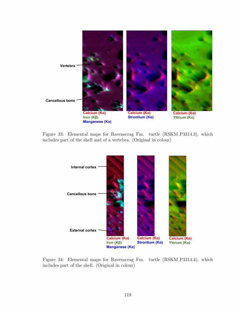
Figure 33: Elemental maps for Ravenscrag Fm. turtle (RSKM P3314.3), whichincludes part of the shell and of a vertebra. (Original in colour)
Figure 34: Elemental maps for Ravenscrag Fm. turtle (RSKM P3314.4), whichincludes part of the shell. (Original in colour)
119
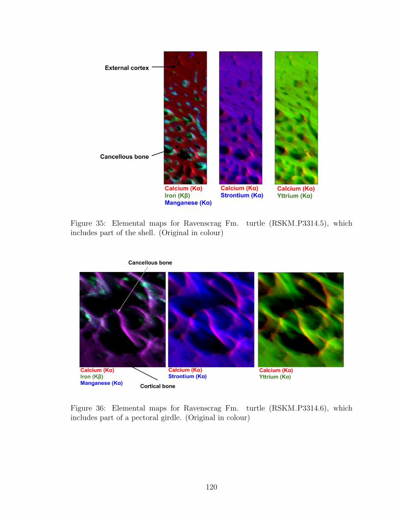
Figure 35: Elemental maps for Ravenscrag Fm. turtle (RSKM P3314.5), whichincludes part of the shell. (Original in colour)
Figure 36: Elemental maps for Ravenscrag Fm. turtle (RSKM P3314.6), whichincludes part of a pectoral girdle. (Original in colour)
120

Figure 37: Elemental maps for Ravenscrag Fm. turtle (RSKM P3314.7), whichincludes part of a limb bone. (Original in colour)
Figure 38: Elemental maps for Frenchman Formation turtle (FF, RSKM P3314.8),which includes part of the shell. Orange arrows indicate examples of regions withinthe marrow spaces with high amounts of iron. (Original in colour)
121
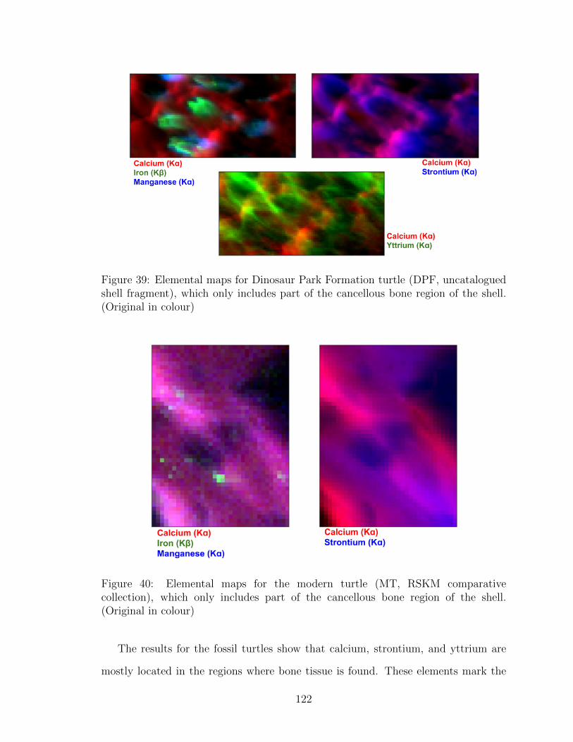
Figure 39: Elemental maps for Dinosaur Park Formation turtle (DPF, uncataloguedshell fragment), which only includes part of the cancellous bone region of the shell.(Original in colour)
Figure 40: Elemental maps for the modern turtle (MT, RSKM comparativecollection), which only includes part of the cancellous bone region of the shell.(Original in colour)
The results for the fossil turtles show that calcium, strontium, and yttrium are
mostly located in the regions where bone tissue is found. These elements mark the
122

details in the microstructure of the bones, such as their Haversian canals and marrow
spaces. Meanwhile, iron and manganese appear mostly within the canals (except for
RSKM P3314.6). In the case of the modern turtle, manganese and calcium seem to
appear in the same regions, with iron particles present in some locations. Although
strontium and calcium appear in the same regions for the modern turtle, the areas
with the highest amount of each of these elements do not correspond to one another.
Yttrium was not detected in the modern turtle specimen.
Using the calcium distribution as a reference, 125 points in each region of the
samples (exterior and interior cortex and cancellous bone, depending on what was
present in each measurement) were selected and their spectra combined and
averaged. The selected regions did not contain osteons canals, marrow spaces, or
areas with abnormally high concentrations of calcium. Figs. 41 to 45 show the
spectra for turtles RSKM P3314.1, RSKM P3314.3, RSKM P3314.4,
RSKM P3314.5 and RSKM P3314.8, with representatives of each mappable shell
region, in order to compare the element quantities among them.
Figure 41: Average spectra for 125 points in the external cortex, cancellous boneand rib of the Ravenscrag Fm. RSKM P3314.1 turtle specimen in linear (left) andlogarithmic (right) scale. Peaks for the elements discussed in this chapter are marked.The red line corresponds to external cortex (EC), black corresponds to cancellous bone(CB) and green corresponds to the section of rib bone (RB). (Original in colour)
123
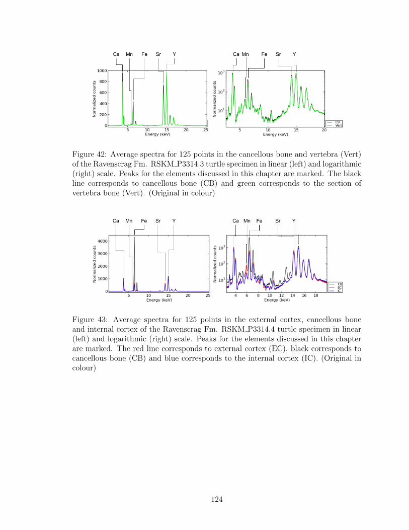
Figure 42: Average spectra for 125 points in the cancellous bone and vertebra (Vert)of the Ravenscrag Fm. RSKM P3314.3 turtle specimen in linear (left) and logarithmic(right) scale. Peaks for the elements discussed in this chapter are marked. The blackline corresponds to cancellous bone (CB) and green corresponds to the section ofvertebra bone (Vert). (Original in colour)
Figure 43: Average spectra for 125 points in the external cortex, cancellous boneand internal cortex of the Ravenscrag Fm. RSKM P3314.4 turtle specimen in linear(left) and logarithmic (right) scale. Peaks for the elements discussed in this chapterare marked. The red line corresponds to external cortex (EC), black corresponds tocancellous bone (CB) and blue corresponds to the internal cortex (IC). (Original incolour)
124

Figure 44: Average spectra for 125 points in the external cortex and cancellous boneof the RSKM P3314.5 Ravenscrag Fm. turtle specimen in linear (left) and logarithmic(right) scale. Peaks for the elements being discussed in this chapter are marked. Thered line corresponds to external cortex (EC) and black corresponds to cancellous bone(CB). (Original in colour)
Figure 45: Average spectra for 125 points in the external cortex and cancellous boneof the FF turtle specimen (RSKM P3314.8) in linear (left) and logarithmic (right)scale. Peaks for the elements being discussed in this chapter are marked. The redline corresponds to external cortex (EC) and black corresponds to cancellous bone(CB). (Original in colour)
The comparison of the spectra with respect to a single region of the bone across
different specimens is shown in figs. 46 and 47 for the cancellous bone and external
cortex, respectively. In these plots, RSKM P3314.5 was chosen to represent the turtles
from RF, because it consists of a similar shell section (without rib bone) to specimens
from the other formations, and unlike RSKM P3314.4, the acquisition time per point
was consistent with that used for the other shells. A comparison including the internal
cortex was not attainable because this region was only mapped in one of the specimens
125
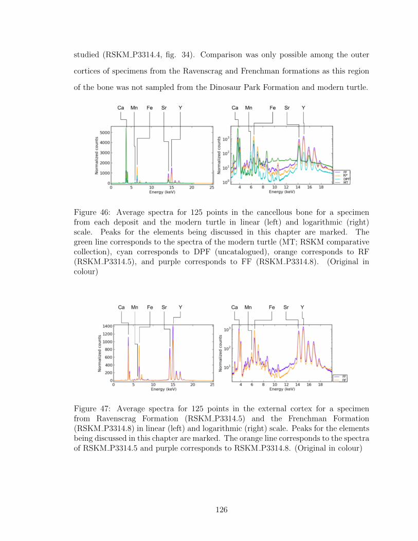
studied (RSKM P3314.4, fig. 34). Comparison was only possible among the outer
cortices of specimens from the Ravenscrag and Frenchman formations as this region
of the bone was not sampled from the Dinosaur Park Formation and modern turtle.
Figure 46: Average spectra for 125 points in the cancellous bone for a specimenfrom each deposit and the modern turtle in linear (left) and logarithmic (right)scale. Peaks for the elements being discussed in this chapter are marked. Thegreen line corresponds to the spectra of the modern turtle (MT; RSKM comparativecollection), cyan corresponds to DPF (uncatalogued), orange corresponds to RF(RSKM P3314.5), and purple corresponds to FF (RSKM P3314.8). (Original incolour)
Figure 47: Average spectra for 125 points in the external cortex for a specimenfrom Ravenscrag Formation (RSKM P3314.5) and the Frenchman Formation(RSKM P3314.8) in linear (left) and logarithmic (right) scale. Peaks for the elementsbeing discussed in this chapter are marked. The orange line corresponds to the spectraof RSKM P3314.5 and purple corresponds to RSKM P3314.8. (Original in colour)
126
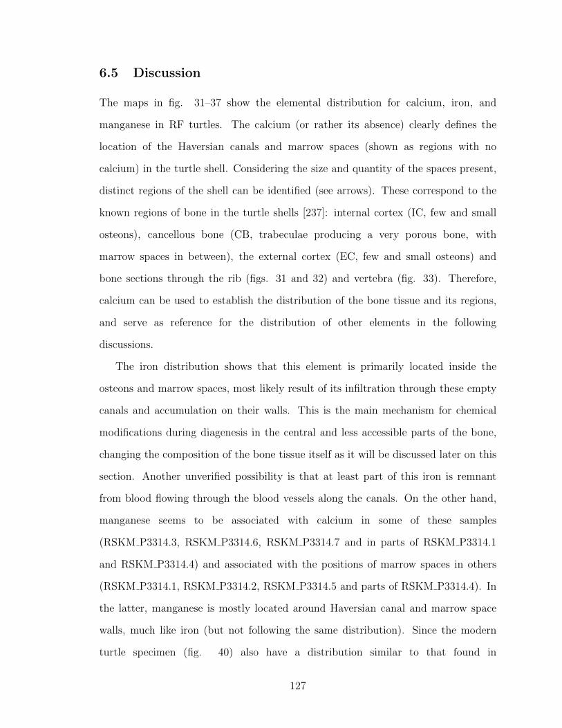
6.5 Discussion
The maps in fig. 31–37 show the elemental distribution for calcium, iron, and
manganese in RF turtles. The calcium (or rather its absence) clearly defines the
location of the Haversian canals and marrow spaces (shown as regions with no
calcium) in the turtle shell. Considering the size and quantity of the spaces present,
distinct regions of the shell can be identified (see arrows). These correspond to the
known regions of bone in the turtle shells [237]: internal cortex (IC, few and small
osteons), cancellous bone (CB, trabeculae producing a very porous bone, with
marrow spaces in between), the external cortex (EC, few and small osteons) and
bone sections through the rib (figs. 31 and 32) and vertebra (fig. 33). Therefore,
calcium can be used to establish the distribution of the bone tissue and its regions,
and serve as reference for the distribution of other elements in the following
discussions.
The iron distribution shows that this element is primarily located inside the
osteons and marrow spaces, most likely result of its infiltration through these empty
canals and accumulation on their walls. This is the main mechanism for chemical
modifications during diagenesis in the central and less accessible parts of the bone,
changing the composition of the bone tissue itself as it will be discussed later on this
section. Another unverified possibility is that at least part of this iron is remnant
from blood flowing through the blood vessels along the canals. On the other hand,
manganese seems to be associated with calcium in some of these samples
(RSKM P3314.3, RSKM P3314.6, RSKM P3314.7 and in parts of RSKM P3314.1
and RSKM P3314.4) and associated with the positions of marrow spaces in others
(RSKM P3314.1, RSKM P3314.2, RSKM P3314.5 and parts of RSKM P3314.4). In
the latter, manganese is mostly located around Haversian canal and marrow space
walls, much like iron (but not following the same distribution). Since the modern
turtle specimen (fig. 40) also have a distribution similar to that found in
127

RSKM P3314.3, RSKM P3314.6 and RSKM P3314.7, and, also, the FF turtle
RSKM P3314.8 (fig. 38) to some extent, the results suggest that specimens
RSKM P3314.1, RSKM P3314.2 and RSKM P3314.5 had a larger Mn intake during
diagenesis. One would expect the infiltrated manganese to accumulate in the osteon
and marrow space walls and, if this concentration is large enough, it would overprint
the original distribution present in the bone tissue, as seen in the modern specimen.
This is confirmed by adjusting the saturation in order to properly view the lower
intensity portion of the distribution (fig. 48). Compared to the saturation used
before (fig. 48-a), the changes in saturation seen in fig. 48-b show that manganese
is, in fact, distributed in the same region where calcium is found, but in a much
smaller quantity than that found in the osteons and marrow spaces. The same effect
is observed in the DPF turtle specimen (fig. 39).
Figure 48: Elemental map for calcium and manganese for the Ravenscrag Formationturtle RSKM P3314.5 with a) the same saturation for Mn used in fig. 35 and b)the saturation changed so that the portion of the distribution with lower intensity isshown in more detail. (Original in colour)
The data provided were not enough to explain the reason(s) for such differences in
the manganese absorption by different specimens. Considering that specimens found
128

in the same formation have very different distributions for this element, one could
establish that differences in age or general location play a less important role than local
variations in the deposit site. For example, animal remains deposited in water would
have a higher probability of absorbing minerals from the neighbouring sediments.
Variations in the remains themselves may also have had a strong influence (e.g., a
shell with cracks and exposed canals early in its diagenetic history would probably
experience more of these changes than intact shell). The fossils in this study were all
found as fragments, but there is no information regarding when in the fossil’s history
such fragmentation took place. The effects of local environment and fossil history are
unique to each specimen, and make it difficult to draw general conclusions
Strontium shows a distribution very similar to that of calcium, since it can
substitute for the latter in bone apatite [179]. In living animals, strontium is mainly
acquired through diet and, thus, its abundance in bones depends on the animals
dietary habits [180]. In fossils, strontium is typically added to the bone during
diagenesis [41], and thus it can also be seen within some Haversian canals and
marrow spaces, where calcium is not present in measurable quantities (it appears as
a blue outline around the canals and spaces; e.g., see orange arrows in fig. 31).
However, when considering the modern turtle strontium distribution (fig. 40), one
can see that, although it also appears in the same areas where calcium is found,
strontium also seems to appear in the osteons, marrow spaces, and other bone areas
where the amount of calcium is smaller. This does not invalidate the previous
discussion about strontium distribution in the fossils being partly controlled by
diagenetic processes, but suggests that there could be a contribution from the
original material in the strontium present inside the Haversian canals and marrow
spaces. This is expected because the blood going through the canals is the main
transport of strontium into the bones. However the relative quantities of strontium
when compared to calcium in fossils is much higher than in the extant turtle shell.
129

This feature is discussed in greater detail later in this chapter, and it suggests that
diagenetic processes are most likely the dominant explanation for the distribution
observed here.
The last maps for the RF turtles show the distribution of yttrium compared to
the distributions of calcium. It is possible to observe in these maps that yttrium has
a behaviour very similar to the one seen for strontium, matching the distribution of
calcium, but it is also present within the osteons and marrow spaces, usually closer
to their walls. While yttrium was detected in all the other samples, no yttrium was
observed in the modern turtle (fig. 40). This results from the fact that yttrium is an
element with a purely diagenetic origin [44]. The maps for the FF RSKM P3314.8
(fig. 38) and DPF (fig. 39) turtles show a similar distribution of yttrium as those for
RF turtles, except for a smaller amount of this element in the bottom half of the DPF
turtle, which is probably due to differences in the deposit and sediment conditions in
these regions during diagenesis.
The maps for the DPF specimen (fig. 39) present distributions very similar to
the RF turtles (figs. 31-37), with calcium and strontium marking the distribution
of bone tissue, while iron is present in larger quantities inside osteons and marrow
spaces. The maps for the FF specimen (fig. 38) indicate what seems to be a very
different distribution, with iron present in the same regions as calcium and strontium.
This is probably due to a smaller amount of diagenetic iron in the fossil, which is not
enough to hide the original distribution in the bone of the animal (i.e., the opposite
effect of what was discussed previously for manganese). In the FF specimen, most
of the osteons and marrow spaces are depleted of iron, with this element distributed
in trace amounts within the bone tissue. Regions with higher concentrations of iron
are present inside some marrow spaces as indicated by the orange arrows in fig. 38.
A similar distribution can be observed for the modern turtle. Iron is present in the
same regions where calcium is present, but it is not exactly correlated and appears
130

in small clusters with higher concentration in some parts of the bones.
Although these measurements were taken with a polychromatic beam, and,
therefore, cannot be easily interpreted in a quantitative fashion, a qualitative
comparison between spectra is still possible. The plots in figs. 41-45 compare
different regions within the same specimen. In all plots, the cancellous bone region
presents a higher amount of iron when compared to the other regions of the shell
(external and internal cortex). This strongly suggests that a large amount of iron
found in these samples is of diagenetic origin and accumulated due to increased
porosity of cancellous bone. The spongy bone in this region increases the surface
area available for exchanges between bone and environment during diagenesis,
increasing the amount of iron absorbed by the bone tissue in this region of the shell.
The only measured region that present a higher iron concentration than the
cancellous bone is the rib section in RSKM P3314.1 (fig. 41), which is also very
porous (as can be seen in its elemental map, fig. 31). The other elements are much
more similar between different bone regions than iron — even for other
diagenetically controlled materials, such as strontium and yttrium. However, the
cancellous bone region still seems to show a slightly larger (or at least equal)
amount of diagenetic elements when compared to external and internal cortices.
The same is true for the calcium concentration.
One can also compare the spectra with respect to a single region of the bone
across different specimens (figs. 46 and 47). The comparison between the cancellous
bone for different turtle specimens (DPF, FF, modern, and the RSKM P3314.5
representative for RF; fig. 46), shows how the relative concentration of calcium in
relation to other elements is overwhelmingly higher for the modern turtle shell. For
the modern specimen, the amount of calcium present is much higher than any other
element, while for the fossils the amount of calcium is comparable to the amounts of
strontium and yttrium, for example. If the modern turtle is taken as a reference,
131

this result suggests that the fossils lost calcium during diagenesis, mostly through
yttrium and strontium replacement. On the other hand, yttrium and strontium
seem to appear in larger relative amounts in the fossil shells.
Another difference between the modern turtle and fossils is the amount of iron
present. It is much higher in the number of counts in the fossils (fig. 46-right, for the
peak corresponding to iron). This suggests that most of the iron measured in these
fossils is the result of diagenetic processes. The RF turtle in particular presents a much
higher iron concentration even with respect to the other fossils, both in its cancellous
bone (fig. 46) and in its external cortex (fig. 47). Since the peaks for the other
elements (Ca, Sr and Y) are fairly similar, this suggests that sedimentary deposits
with certain characteristics favoured iron absorption by this shell when compared to
the other fossils.
6.6 Conclusions
The results presented in this chapter show maps comparing different specimens of
turtles from the Ravenscrag Formation, Frenchman Formation, and the Dinosaur
Park Formation with material from a modern turtle. The elemental maps and XRF
spectra show clear differences not only between deposits, but also among specimens
from the same formation, and between different bone layers in the same specimen.
Here, it is shown that the cancellous bone in turtle shells undergoes more chemical
taphonomic alterations than the more compact bone layers (external and internal
cortices), due to its higher porosity. It is also shown that local differences in the
deposit’s environment can some times have similar or greater effects than those found
between specimens from different formations and ages. The results seen here for
the turtles suggest that the same is possibly true for fossils from other species. The
characteristics of fossils are difficult to generalize, because they depend strongly on
the local conditions of the deposit. As a result, fossils found very close to one another
132

with the same approximately the same age can have completely different taphonomic
alterations.
Furthermore, the manganese distribution results show that all fossil bones start
with a distribution of manganese consistent with the bone tissue distribution in
modern turtle shell (i.e., there is strong potential that original manganese can still
be found in the fossils). This was shown for the Ravenscrag Formation turtle
RSKM P3314.5 (fig. 48), for example. During diagenesis, infiltration of minerals
through the canals in the shells causes the accumulation of manganese in the osteon
and marrow space walls, as well as the increase of its amount in the bone tissue due
to absorption effects (see fig. 46 for a comparison between the amount of manganese
in the modern turtle and the fossils). Thus, the presence of large amounts of
manganese in the osteon and marrow space walls can be used as a criterion to
qualitatively compare the levels of alteration or replacement between different
bones. If there is a large quantity of manganese, then the bone has potentially
endured significant chemical changes during diagenesis.
133

7 Chemical diagenesis of individual structures in
hadrosaurid skin layer
7.1 Abstract
Most fossils from deep time are preserved remains of animals’ hard parts (i.e.,
tissues already mineralized while the animals are alive, such as bones, and teeth).
Rarely, the conditions are such that the preservation of soft tissues (such as muscle
and integument) is possible. Here, I study the chemistry of a fossilized hadrosaurid
(Edmontosaurus sp.) skin with detailed anatomical preservation, as part of a larger
project involving other researchers. The research previously performed in this
specimen had shown skin-like layers formed by substructures [245]. My goal, in
particular, was to tentatively study the chemistry of a single example of the
substructures in order to hypothesize on the mechanisms behind their preservation.
The results (section 7.4) show the presence of carbon, calcium and iron within the
substructure. Calcium, in the form of carbonate, was found in large quantity in the
region surrounding the substructure. This occurrence was probably a result of
mineral infiltration, and calcium is also present in smaller amounts within the
structure. This could be the result of an early mineralization process that outpaced
microbial decay. The mineralization process contributed to the highly-detailed
preservation of the skin specimen and for the potential entrapment of molecules
with biological origin. The extent of this preservation is observed through the
analysis of the carbon form identified in the skin. Iron (in Fe(III) oxidation state)
was found, oddly, only in the middle of the substructure, and may also be part of
the mechanism that resulted in the preservation of this specimen.
134
7.2 Introduction
Hadrosaurids are members of the clade Ornithopoda. This clade includes all
ornithischian dinosaurs that are more closely related to the hadrosaurid
Edmontosaurus than to the ceratopsian Triceratops [246]. Ornithopoda was once
used to group all dinosaurs that did not belong to one of the known groups, but this
is not the case anymore. Most ornithopods possess kinetic skulls, ventrally offset
premaxillary and jaw joints relative to the maxillary tooth row, a mandibular
fenestra that is closed or reduced, and a rectangular obturator process on the
ischium [246]. The most primitive members of this clade are the hypsilophodontids
known to have lived in the Late Jurassic, but believed to exist since the Middle
Jurassic at least. This group included the genera Hypsilophodon and Thescelosaurus
and existed until the end of the Cretaceous [246].
Within Ornithopoda, hadrosaurids are part of the clade Iguanodontia, which
included ornithopods more closely related to Edmontosaurus than to
Thescelosaurus. Iguanodontia is characterized by a transversely expanded
premaxilla lacking teeth, a deep dentary with parallel dorsal and ventral margins, a
missing phalanx from digit III in their hands and a deep and transversely
compressed anterior process in the pubis [246]. The earliest evidence of a member of
the Iguanodontia is a single femur from the Middle Jurassic in Europe [246].
More specifically, hadrosaurids are members of the clade Hadrosauroidea, which
is part of Iguanodontia and includes the family Hadrosauridae. This clade includes
the subfamilies Hadrosaurinae and Lambeosaurinae as well as other basal taxa [246].
hadrosaurids are members of the Hadrosaurinae subclade and are a very well-known
group, with fossils having been found in many regions of the world, including nearly
complete skeletons, skin fossils, remains of eggs, embryos, hatchlings and coprolites
[54, 247, 248, 249, 250]. They were large animals, estimated to be between 7 and 12
metres long and having an average mass of 3 tons, with some species that were much
135

heavier. They were characterized by using both bipedal and quadrupedal postures
and by highly modified tooth rows of dental batteries with as many as sixty teeth
organized in files of 3 to 5 closely packed teeth each [246].
The most commonly preserved fossils are structures that were mineralized when
the animal was alive, such as the teeth and bones. However, soft-tissues are also
rarely preserved. The most common soft-tissue preservation is of structures made
of more durable materials such as the protein keratin, which is the main component
of external skin layers (scales), claws and feathers [251]. Animal skin has roles that
include protection (it must be able to resist abrasion), defense against microbial
invasion, and maintaining water balance. This is achieved through the presence of
keratin (present as alpha and beta forms in dinosaurs [251]) as the main structure of
the skin external layers. Keratin possesses great durability and is insoluble in water,
making it resistant to decay through hydrolytic damage [251].
Even though dinosaur skin has properties that can lead to preservation in the
fossil record, most specimens found have been classified as only skin impressions in
sediments (e.g. [252] and references therein). This can still lead to an understanding
of how dinosaur skin dealt with dermal pathology [253], and the establishment of
a set of criteria to identify skin impressions from other phenomena that can mimic
these impressions [254]. However, rare occurrences of actual fossilized skins have also
been documented. These specimens have been used to provide insights on dinosaur
behaviour and physiology.
A deep cross section through the dermis of a Psittacosaurus found in the Jehol
Group, China, showed visible collagenous fiber layers [255]. The study of this
specimen indicates that 25 well-preserved and 15 poorly-preserved fiber layers were
estimated to be present, suggesting a very thick skin. Also, the fibers in the layers
were organized into left- and right-handed geodesic helices, which would have
improved the skin’s resistance to stresses and strains. This suggests that this
136

dinosaur’s skin was highly adapted for protection [255].
Another example of fossilized skin was found in an exceptionally preserved three-
dimensional specimen of nodosaurid ankylosaur (Borealopelta markmitchelli) from
the Early Cretaceous in Alberta, Canada [56]. Mass spectroscopy studies of this
specimen showed the preservation of melanin, revealing a lighter pigmentation on the
animal’s parascapular spines and a pattern of countershading on the animal’s body.
This pigmentation suggested that the spines were probably used for display while the
larger-scale color patterns were an adaptation against predation [56].
The most relevant previous fossil discovery to the specimen described herein is a
hadrosaurid (Edmontosaurus sp.) skin fossil from the Hell Creek Formation (North
Dakota, U. S. A.) [54]. This specimen was described as containing partially
preserved epidermal microstructures, including the mineralized skin cell boundaries.
FTIR measurements suggested the presence of compounds with amide groups [54].
The exceptional preservation was explained by the rapid burial and mineralization,
which outpaced tissue decay and preserved structures with high fidelity. The
mineralization was assisted by the presence of bicarbonate in the system due to an
anoxic environment with high methanogenesis, and by the dissolved reduced iron
and rock fragments (caused by reducing porewaters resulting from the decay of
plant material). The reduced iron-rich solution rapidly replaced soft tissues with
carbonate minerals [54].
Previous measurements collected from the hadrosaurid under study by other
members of the research team indicated the presence of carbon-rich layers that
appear to be composed of substructures with layering patterns similar to those
found in epithelial tissue of chicken leg skin. Assuming this to be true, I tentatively
selected one of these supposed substrutures for further studies. The aim was to
chemically characterize a single substructure in order to possibly obtain information
relevant to its preservation mechanism. This is the focus of the work discussed in
137

this chapter.
7.3 Material and methods
The measurements described in this chapter are part of a series of measurements
taken on samples of the same hadrosaurid skin, and performed by different members
of the research group, including myself, using several different techniques. The results
presented here are based on the measurements performed as part of my thesis research
and developed by me, but will also include some of the other results, where they
are relevant to the discussion. Section 7.3.1 provides a description of the specimen
used in this study along with some information concerning the location where it was
discovered. The methodology used for the measurements discussed in this chapter is
described in section 7.3.2.
7.3.1 Specimen and geological settings
The specimen used in this study is a sheet of fossilized integument (skin) found
associated with UALVP 53290 [245]. UALVP 53290 is an incomplete
articulated-to-associated hadrosaurid skeleton, tentatively classified as
Edmontosaurus cf. regalis (the only hadrosaurid species known from this
stratigraphic interval) [245]. The skeleton was found in the Red Willows Fall
locality of the Upper Cretaceous Wapiti Formation near Grande Prairie (Alberta,
Canada), and consists of most of the thoracic region, forelimb and pelvic elements,
among other bones. The integument was associated with the forelimbs of UALVP
53290, presumably from the dorsal and anterior surface of the forearm [245]. The
skin presented scales identical to the ones found in the upper arm regions of other
Edmontosaurus specimens (e.g., [54]) [245].
The Wapiti Formation is a nonmarine deposit of interbedded fluvial sandstone,
siltstone and mudstone deposited during the early Campanian to the Late
138

Maastrichtian [256]. The formation can be divided into five stratigraphic units, as
described in [256], unit 4 being the one where the hadrosaurid specimen was found
[245]. Unit 4 deposits consist of repeating sequences of crevasse-splay, muddy and
organic-rich overbank deposits, and minor sandy channel fills [256]. The stacking
pattern suggests a fluvial environment, and together with common coal seams, it
indicates the presence of high-water table conditions and highly vegetated, poorly
drained grounds [257]. Many fossils have been found in the carbonaceous mudstone
layers of this unit, including duck-billed and horned dinosaurs (remains and tracks),
and insects in amber (see [256] and references therein).
7.3.2 Methodology
A piece of a pristine fossilized hadrosaurid skin (from skeleton UALVP 53290) with
the attached sediment matrix was sectioned using a microtome (Leica EM UC7) in
a water bath with the goal of obtaining a slice of 100 nm thickness. However, due
to the brittleness of the specimen, this process resulted in flakes and debris of the
sample. These fragments were collected and deposited on a silicon nitride membrane
and air-dried at room temperature before the measurements.
Scanning transmission X-ray microscopy (STXM) measurements were taken at
the Soft X-ray Spectromicroscopy Beamline (SM) [258, 259] at the Canadian Light
Source. This technique, as the name suggests, is performed in transmission mode and
results in a series of XAS spectra: one for each pixel measured in the selected region
of the sample. This beamline uses a beam produced by a 75 mm generalized Apple
II Elliptically Polarizing Undulator, with energy range between 130 and 2700 eV and
spot size on the sample for STXM measurements of 30 nm, with wavelength selected
by a slit-less plane grating monochromator with single grating substrate with three
stripes.
A carbonyl map of the region with the skin layer (fig. 49-left) was used to
139
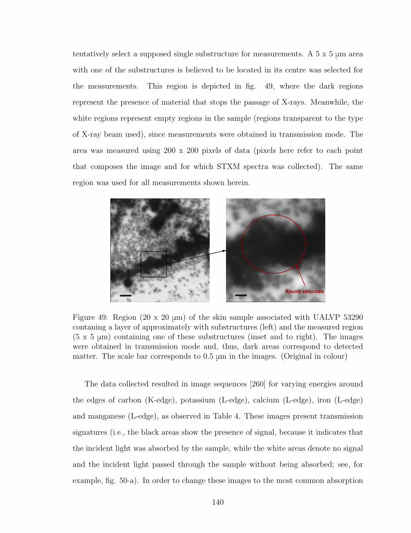
tentatively select a supposed single substructure for measurements. A 5 x 5 μm area
with one of the substructures is believed to be located in its centre was selected for
the measurements. This region is depicted in fig. 49, where the dark regions
represent the presence of material that stops the passage of X-rays. Meanwhile, the
white regions represent empty regions in the sample (regions transparent to the type
of X-ray beam used), since measurements were obtained in transmission mode. The
area was measured using 200 x 200 pixels of data (pixels here refer to each point
that composes the image and for which STXM spectra was collected). The same
region was used for all measurements shown herein.
Figure 49: Region (20 x 20 μm) of the skin sample associated with UALVP 53290contaning a layer of approximately with substructures (left) and the measured region(5 x 5 μm) containing one of these substructures (inset and to right). The imageswere obtained in transmission mode and, thus, dark areas correspond to detectedmatter. The scale bar corresponds to 0.5 μm in the images. (Original in colour)
The data collected resulted in image sequences [260] for varying energies around
the edges of carbon (K-edge), potassium (L-edge), calcium (L-edge), iron (L-edge)
and manganese (L-edge), as observed in Table 4. These images present transmission
signatures (i.e., the black areas show the presence of signal, because it indicates that
the incident light was absorbed by the sample, while the white areas denote no signal
and the incident light passed through the sample without being absorbed; see, for
example, fig. 50-a). In order to change these images to the most common absorption
140
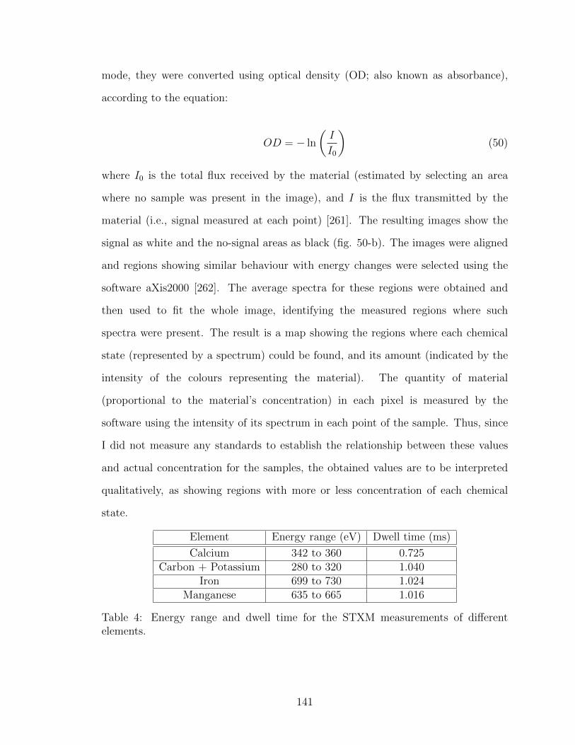
mode, they were converted using optical density (OD; also known as absorbance),
according to the equation:
OD = − ln
(I
I0
)(50)
where I0 is the total flux received by the material (estimated by selecting an area
where no sample was present in the image), and I is the flux transmitted by the
material (i.e., signal measured at each point) [261]. The resulting images show the
signal as white and the no-signal areas as black (fig. 50-b). The images were aligned
and regions showing similar behaviour with energy changes were selected using the
software aXis2000 [262]. The average spectra for these regions were obtained and
then used to fit the whole image, identifying the measured regions where such
spectra were present. The result is a map showing the regions where each chemical
state (represented by a spectrum) could be found, and its amount (indicated by the
intensity of the colours representing the material). The quantity of material
(proportional to the material’s concentration) in each pixel is measured by the
software using the intensity of its spectrum in each point of the sample. Thus, since
I did not measure any standards to establish the relationship between these values
and actual concentration for the samples, the obtained values are to be interpreted
qualitatively, as showing regions with more or less concentration of each chemical
state.
Element Energy range (eV) Dwell time (ms)
Calcium 342 to 360 0.725Carbon + Potassium 280 to 320 1.040
Iron 699 to 730 1.024Manganese 635 to 665 1.016
Table 4: Energy range and dwell time for the STXM measurements of differentelements.
141

Figure 50: Mapped region (5 x 5 μm) of hadrosaurid skin associated with UALVP53290 in a) transmission mode and b) absorption (O. D.) mode. .
7.4 Results
In the region of interest, STXM measurements were taken in the energy regions
corresponding to the edges for calcium, carbon and potassium, iron and manganese
(see table 4). The stacks of images were then analyzed for each element and the
different XAS spectra were obtained for different regions in the measured area (figs.
51, 52, 53 and 54, for calcium, carbon, iron and manganese, respectively). Manganese
and potassium could not be detected in the measured region.
Figure 51: Calcium XAS spectra for different regions of the substructures found inthe UALVP 53290 skin layer. The colour of each spectrum (right) corresponds to thecolour of the region in the image (left), where white areas represent a strong signaland black represents no signal. The vertical line represents the energy in the plot forwhich the image in the left was taken. (Original in colour) .
142
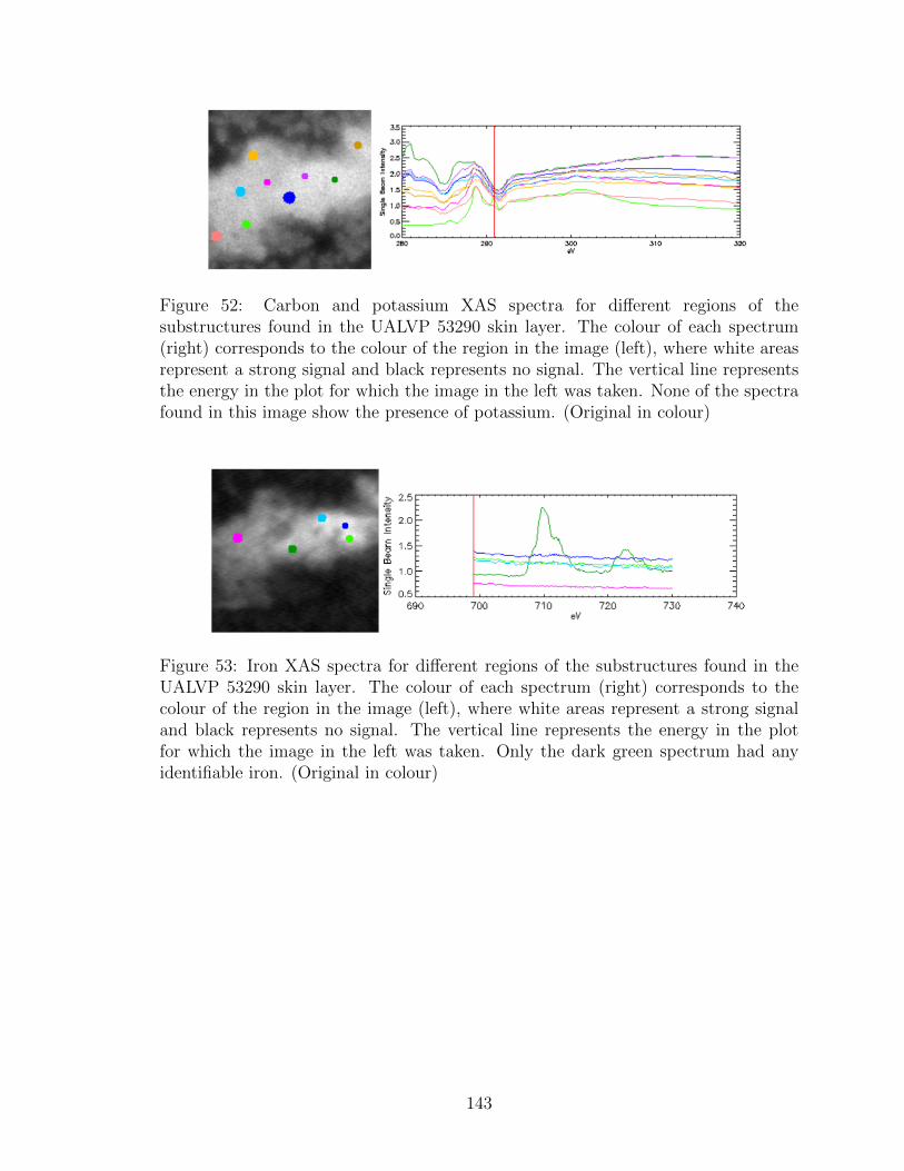
Figure 52: Carbon and potassium XAS spectra for different regions of thesubstructures found in the UALVP 53290 skin layer. The colour of each spectrum(right) corresponds to the colour of the region in the image (left), where white areasrepresent a strong signal and black represents no signal. The vertical line representsthe energy in the plot for which the image in the left was taken. None of the spectrafound in this image show the presence of potassium. (Original in colour)
Figure 53: Iron XAS spectra for different regions of the substructures found in theUALVP 53290 skin layer. The colour of each spectrum (right) corresponds to thecolour of the region in the image (left), where white areas represent a strong signaland black represents no signal. The vertical line represents the energy in the plotfor which the image in the left was taken. Only the dark green spectrum had anyidentifiable iron. (Original in colour)
143

Figure 54: Manganese XAS spectra for different regions of the substructures found inthe UALVP 53290 skin layer. The colour of each spectrum (right) corresponds to thecolour of the region in the image (left), where white areas represent a strong signaland black represents no signal. The vertical line represents the energy in the plot forwhich the image in the left was taken. Manganese was not found in any region of themeasured area. (Original in colour)
In fig. 51 the presence of two different chemical states for calcium are apparent
within the sample: the one in red (referred to as calcium-1 hereafter), and the other
corresponding to the other colours (calcium-2 hereafter). These spectra can be used
to fit the spectra for each point in the image, assuming each point’s spectrum is a
linear combination of the individual spectra for each chemical state. The fitting is
done in order to identify the specific areas in the sample where each state can be
found (fig. 55). These regions were used to create a mask and select the areas in the
sample where each of the spectra are stronger, thus calculating the average spectrum
for each of these areas. Details can be seen in fig. 56, and the peaks from each
spectrum are listed in table 5.
144

Figure 55: Map showing the distribution of the two different states of calcium in fossilskin associated with UALVP 53290, where a) shows the distribution of the spectrumfound in red in fig. 51 (calcium 1), b) shows the distribution of the other spectrum(calcium 2) and c) shows a combination of both distributions. The circle in a) showsthe approximated region where the substructure is believed to be. The arrow showsthe region of strong calcium 1. (Original in colour)
Figure 56: Average spectra of calcium 1 (blue) and calcium 2 (red) in fossil skinassociated with UALVP 53290, calculated based on the regions where the spectra arefound. Blue arrows point at the main peaks of the spectra, while black arrows pointat the secondary peaks. The red arrow points at detail at the second main peak,where two “bumps” can be observed. (Original in colour)
145

Spectrum Peaks (eV)
Calcium 1 347.7, 348.2, 348.8, 350.1, 352.2, 353.4Calcium 2 347.8, 349.0, 349.9, 350.1, 352.3, 353.1, 353.4
Table 5: Calcium peaks for each spectrum in fig. 56.
Fig. 55 shows that the distribution of the two states of calcium are different from
one another. Even though both seem to be present in small quantities in the whole
measured region, the areas where they are in larger quantities are different depending
on the state. For calcium 1, the highest amounts can be found in a “lens” in the
bottom, left corner of the mapped region (see white arrow), followed by some presence
in the area where the substructure is found. Meanwhile, the calcium 2 distribution
shows its highest amounts approximately in the middle and in the surrounding areas
of the structure. The fact that these two states of calcium are different is also visible
when comparing their spectra in fig. 56. In this image, the position and relative
intensity of the peaks (also seen in table 5) for the two spectra are clearly different.
Fig. 52 shows the presence of three types of carbon spectra present in the mapped
region, exemplified by the spectrum in dark green (referred to as carbon-1 hereafter),
the one in pink (carbon-2 hereafter) and the one in light green (carbon-3 hereafter).
The distribution of these three states can be seen in fig. 57 and the average spectrum
for each distribution is shown in fig. 58. Table 6 shows the position of the peaks
identified in the spectra shown in fig. 58.
146

Figure 57: Map showing the distribution of the three different states of carbon infossil skin associated with UALVP 53290, where a) shows the distribution of carbon-1, b) shows the distribution of carbon-2, c) shows the distribution of carbon-3 and d)shows a combination of all distributions. (Original in colour)
Figure 58: Average spectra of carbon 1, 2 and 3 in fossil skin associated with UALVP53290, calculated based on the regions where the spectra are found. (Original incolour)
147

Spectrum Peaks (eV)
Carbon 1 288.5Carbon 2 288.6Carbon 3 285.6, 288.6, 290.7
Table 6: Carbon peaks for each spectrum in fig. 58.
The three states of carbon detected show very different distributions in the
measured region, as seen in fig. 57. Carbon 1 appears mostly in the region close to
the border of the substructure and in small zones between them. Carbon 2 appears
with higher intensity in the middle of the substructure, while carbon 3 seems to
have a more homogeneous distribution, with some higher amounts in the areas
surrounding the substructure. These carbon states are clearly different from each
other, as can be seen in fig. 58.
Fig. 53 shows that only one spectrum of iron seems to be present in the mapped
regions. The corresponding map showing its distribution can be seen in fig. 59 and
the average iron spectrum based on this distribution is presented in fig 60. Iron is
only present in one state in the mapped region, and it is only present in a small area
approximately in the middle of the substructure (fig. 59).
Figure 59: Map showing the distribution of the only measured state of iron in fossilskin associated with UALVP 53290 as seen in the green spectrum of fig. 53. (Originalin colour)
148

Figure 60: Average spectrum of iron in fossil skin associated with UALVP 53290,calculated based on the regions where the spectrum are found. (Original in colour)
Maps comparing the distribution of different identified elements in the regions
under study can be observed in figs. 61 and 62, using carbon-1 and carbon-2,
respectively. A similar map for carbon-3 was not produced because its distribution
covers most of the map and the only visible feature is an increase in intensity in the
same region where the calcium is abundant.
Figure 61: Maps comparing the distributions of carbon-1, iron and a) calcium-1 andb) calcium-2 in fossil skin associated with UALVP 53290. (Original in colour)
149

Figure 62: Maps comparing the distributions of carbon-2, iron and a) calcium-1 andb) calcium-2 in fossil skin associated with UALVP 53290. (Original in colour)
7.5 Discussion
The main peak of L3-edge calcite (at 350.1 eV) was arbitrarily set at the energy of
349.3 eV, as was done in [263], in order to compare the peak positions with the
standards described in this reference. Using the information displayed in table 5,
this results in peaks at positions (in eV): 346.9, 347.4, 348.0, 349.3, 351.4 and 352.6
for calcium-1, being a perfect match for the described calcite (CaCO3) spectrum.
Therefore, the material so far called calcium-1 can be identified as calcite, and is
likely associated with sedimentary materials surrounding the skin. Fig. 55 shows
that calcite distribution sits in larger quantities outside the substructure, forming
an egg-shaped structure encapsulating it (see white outline in the figure). It is
probably a calcite-rich crystal from the sedimentary rock. The distribution also
shows that calcite is present within the substructure in smaller quantities. The
presence of calcite within the substructure could be the result of an
early-mineralization process, which may have contributed to the preservation of
these structures [7]. However, calcium carbonates are not often known for detailed
preservation of soft-tissues in taphonomic studies: this preservation is usually a
result of calcium phosphate deposition (phosphatization) [39]. The two processes
150
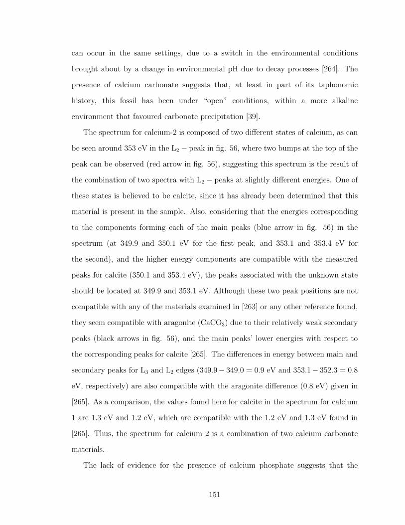
can occur in the same settings, due to a switch in the environmental conditions
brought about by a change in environmental pH due to decay processes [264]. The
presence of calcium carbonate suggests that, at least in part of its taphonomic
history, this fossil has been under “open” conditions, within a more alkaline
environment that favoured carbonate precipitation [39].
The spectrum for calcium-2 is composed of two different states of calcium, as can
be seen around 353 eV in the L2 − peak in fig. 56, where two bumps at the top of the
peak can be observed (red arrow in fig. 56), suggesting this spectrum is the result of
the combination of two spectra with L2 − peaks at slightly different energies. One of
these states is believed to be calcite, since it has already been determined that this
material is present in the sample. Also, considering that the energies corresponding
to the components forming each of the main peaks (blue arrow in fig. 56) in the
spectrum (at 349.9 and 350.1 eV for the first peak, and 353.1 and 353.4 eV for
the second), and the higher energy components are compatible with the measured
peaks for calcite (350.1 and 353.4 eV), the peaks associated with the unknown state
should be located at 349.9 and 353.1 eV. Although these two peak positions are not
compatible with any of the materials examined in [263] or any other reference found,
they seem compatible with aragonite (CaCO3) due to their relatively weak secondary
peaks (black arrows in fig. 56), and the main peaks’ lower energies with respect to
the corresponding peaks for calcite [265]. The differences in energy between main and
secondary peaks for L3 and L2 edges (349.9− 349.0 = 0.9 eV and 353.1− 352.3 = 0.8
eV, respectively) are also compatible with the aragonite difference (0.8 eV) given in
[265]. As a comparison, the values found here for calcite in the spectrum for calcium
1 are 1.3 eV and 1.2 eV, which are compatible with the 1.2 eV and 1.3 eV found in
[265]. Thus, the spectrum for calcium 2 is a combination of two calcium carbonate
materials.
The lack of evidence for the presence of calcium phosphate suggests that the
151

preservation of skin layers in the hadrosaurid specimen is not a result of
phosphatization, and that the presence of calcium carbonate cannot be explained by
the pH switch described previously and discussed in [264]. The precipitation of
phosphates would be favoured over that of carbonates if the conditions were
“closed”, resulting in an anoxic environment with an acidic pH. The absence of
phosphatization in spite of the presence of a nearby source of phosphorous (the
animal’s carcass), and the presence of calcium carbonate instead, indicates different
taphonomic conditions during its mineralization stage. The skin specimen was
found in an area believed to have exhibited freshwater conditions, with a high water
table, high amount of vegetation and poorly drained soils [257]. This was an “open”
environment, with presence of water and decaying vegetation, creating conditions
similar to the ones described in [54] (see also section 7.1.2). The setting would
favour the rapid replacement of soft tissue with carbonate minerals. The presence of
substructures believed to be remnants of the original tissues suggest the
replacement was faster than microbial decay. The rapid mineralization resulted in
the high-fidelity preservation of skin substructures. As discussed in the following
paragraphs, rapid mineralization ensured that products from organic molecules were
preserved within the fossil.
The position of the peaks measured in the spectra for carbon-1 and 2 are
compatible to the ones attributed to the carboxyl group, which should appear
between 288.0 and 288.7 eV [266]. These are organic forms of carbon. The presence
of organic carbon in the hadrosaurid skin layer suggests that I could be measuring
the remains of original organic material from the dinosaur, or material from the
decay process, or maybe subsequent biological activity. However, with the use of the
techniques attempted here alone, it is not possible to determine exactly which
compound is being measured and, therefore, it is not possible to exactly determine
its source.
152

For carbon-3, the spectrum shows the presence of the same peak discussed in
the previous paragraph, corresponding to the presence of the carboxyl group. The
peak at lower energies (285.6 eV) is compatible with an aromatic (C = C) functional
group that could potentially have originated from an biological process. The peak at
290.7 eV is most likely indicative of carbonates [267], as suggested by the previous
observation of calcite in the sample. In fact, the region in the map shown in fig. 57-c
with the highest concentration of this carbon state matches the area where calcite
was predominant in the sample (fig. 55-a).
Although not presented in this thesis, other measurements have been performed
on this specimen by other members of the research team using other techniques such
as Fourier-transform infrared spectroscopy (FTIR). The measurements through this
technique also strongly support the evidence for the presence of organic material in
the regions of the specimen where the skin layer is located [245]. The unpublished
data further corroborates the discussion presented here. Ultimately, it supports the
idea that the observed carbon is the result of some biological process experienced by
the animal after its death.
The main peak in the spectrum shown in fig. 60 is found at 709.8 eV, indicating
iron in Fe(III) oxidation state [260]. Although the mechanism that led to this form
of iron in the sample is not understood, the presence of Fe(III) has been associated
with exceptional preservation of fossils in the past, especially with preservation of
soft-tissues in dinosaurs [7]. The fact that its distribution indicates a concentration
of this compound in the skin layer substructures, and nowhere else in the mapped
region, seems to strongly corroborate this hypothesis.
The maps in figs. 61 and 62 show that the presence of Fe(III) is concentrated
within the region in the center of the substructure, which also corresponds to the
highest concentrations of organic carbon in both images. In all the maps it is
possible to see that calcium carbonate is also present in small quantities within the
153

substructure, but is present in higher amount in the regions surrounding the
structure. This calcium carbonate distribution is probably the result of infiltration
of cementing minerals through voids in the layer.
7.6 Conclusions
The results shown here suggest that the exceptional preservation of the skin layers
from a hadrosaurid is the result of an unknown mechanism involving the presence of
Fe(III) in combination with the rapid mineralization caused by the replacement of
soft tissues with carbonate minerals. The effect of this iron state has already been
described in the literature as being related to the preservation of dinosaur soft
tissues. Mineralization outpacing microbial decay was responsible for a highly
detailed preservation of the morphological structure of the skin layer. It was also
responsible for the preservation of molecules of biological origin identified by the
presence of organic carbon groups in the region where one of the substructures that
make up the skin layer is found. Although these organic compounds cannot be
precisely identified, they strongly suggest the presence of preserved tissues when
combined with the structured distributions observed.
Regardless of the processes involved, the findings described here present evidence
that the layers of material identified in the hadrosaurid skin retain structure that
reflect the preservation of fossilized skin layers. This is backed by both the physical
structure of these layers, similar to those found in skins of living avian species, and
its chemical composition.
154
8 Synchrotron applied to taphonomic studies
8.1 Abstract
The previous chapters discuss the results of the research involving the application
of synchrotron-based techniques to taphonomic studies concerning different animal
groups, types of fossils and different types of fossilized tissues. The goal of this
chapter is to combine these results and analyses to obtain information about fossils
in general, their differences and similarities, and the possible associations they may
have that can be explored using these techniques.
8.2 Introduction
Several different specimens were studied in the previous sections. Here I present
comparative analyses involving the bones and tendon previously discussed with
respect to the relative concentration of the elements of interest and their
correlations. Please, refer to these sections for specifics of individual projects,
specimens, and techniques covered in this synthesis.
8.3 Results
The peak area of iron, manganese, strontium and yttrium relative to calcium was
calculated for the bone specimens mentioned in the previous chapters, namely T. rex,
hadrosaur, swan, and turtle (extant and fossil) bones, using the equation
Relamount =AreaelementAreacalcium
(51)
where Areaelement refers to integrated counts under the peak of the element being
calculated (iron, manganese, strontium, or yttrium), and Areacalcium is the integrated
counts under the peak correponding to calcium. These areas for turtle shells and
155

dinosaur bones are listed on table 7. They were calculated based on a selected area
of the map containing only bone tissue. It is important to notice, however, that
what is being computed here is not the relative concentration, but the relative area of
the peaks. This distinction is necessary because the concentration for each element
was not obtained and the integrations under the peaks identified in each spectrum
are only proportional to the actual element concentration and do not give the real
concentrations. The values used for the calculations include the Ca K-alpha and K-
beta peaks (3,691.68 eV and 4,012.7 eV) for the area of calcium, Fe K-beta (7,057.98
eV) for iron and K-alpha peaks for the other elements (5,898.75 eV for manganese,
14.165 eV for strontium and 14,958.4 eV for yttrium). The Fe K-alpha peak was not
used because it is located at the same energy as the Mn K-beta peak. Therefore, since
K-alpha and K-beta peak intensities are proportional, there is no loss of information
by selecting one or the other. In this way, the results obtained for the area of iron
are independent of the area of manganese present in the sample.
Sample Iron Manganese Strontium Yttrium
Swan femur 0.112043 0.0392676 1.62247 -Extant turtle 0.00350424 0.00228511 0.105049 -
Hadrosaur tendon 0.339417 0.151169 0.667739 1.56149T. rex rib (fig. ) 0.0779487 0.83652 0.530047 0.221752T. rex rib (fig. ) 0.412866 2.61926 0.381296 0.224441T. rex vertebra 0.109736 0.26276 0.457367 0.37145
Turtle DPP 0.344965 0.579493 1.03543 0.365736Turtle FF 0.093124 0.0407651 1.18513 1.99849Turtle T1 0.210233 0.0718282 1.22575 1.57938
Turtle RF RSKM P3314.5 1.36944 0.256526 0.798125 1.24094
Table 7: Relative areas of Fe, Mn, Sr and Y relative to Ca for dinosaur bones andturtle shells used in the research presented in previous chapters.
The distribution of the ratio between iron, manganese, strontium, and yttrium in
relation to calcium are shown in figs. 63-66. For these plots, only four specimens (T.
rex rib (fig. 6), T. rex rib (fig. 7), DPP turtle and RF RSKM P3314.5 turtle) were
chosen as representative of the other samples.
156
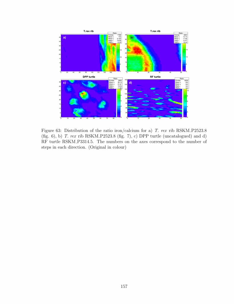
Figure 63: Distribution of the ratio iron/calcium for a) T. rex rib RSKM P2523.8(fig. 6), b) T. rex rib RSKM P2523.8 (fig. 7), c) DPP turtle (uncatalogued) and d)RF turtle RSKM P3314.5. The numbers on the axes correspond to the number ofsteps in each direction. (Original in colour)
157
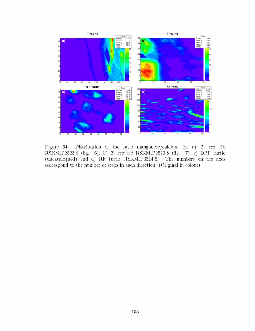
Figure 64: Distribution of the ratio manganese/calcium for a) T. rex ribRSKM P2523.8 (fig. 6), b) T. rex rib RSKM P2523.8 (fig. 7), c) DPP turtle(uncatalogued) and d) RF turtle RSKM P3314.5. The numbers on the axescorrespond to the number of steps in each direction. (Original in colour)
158
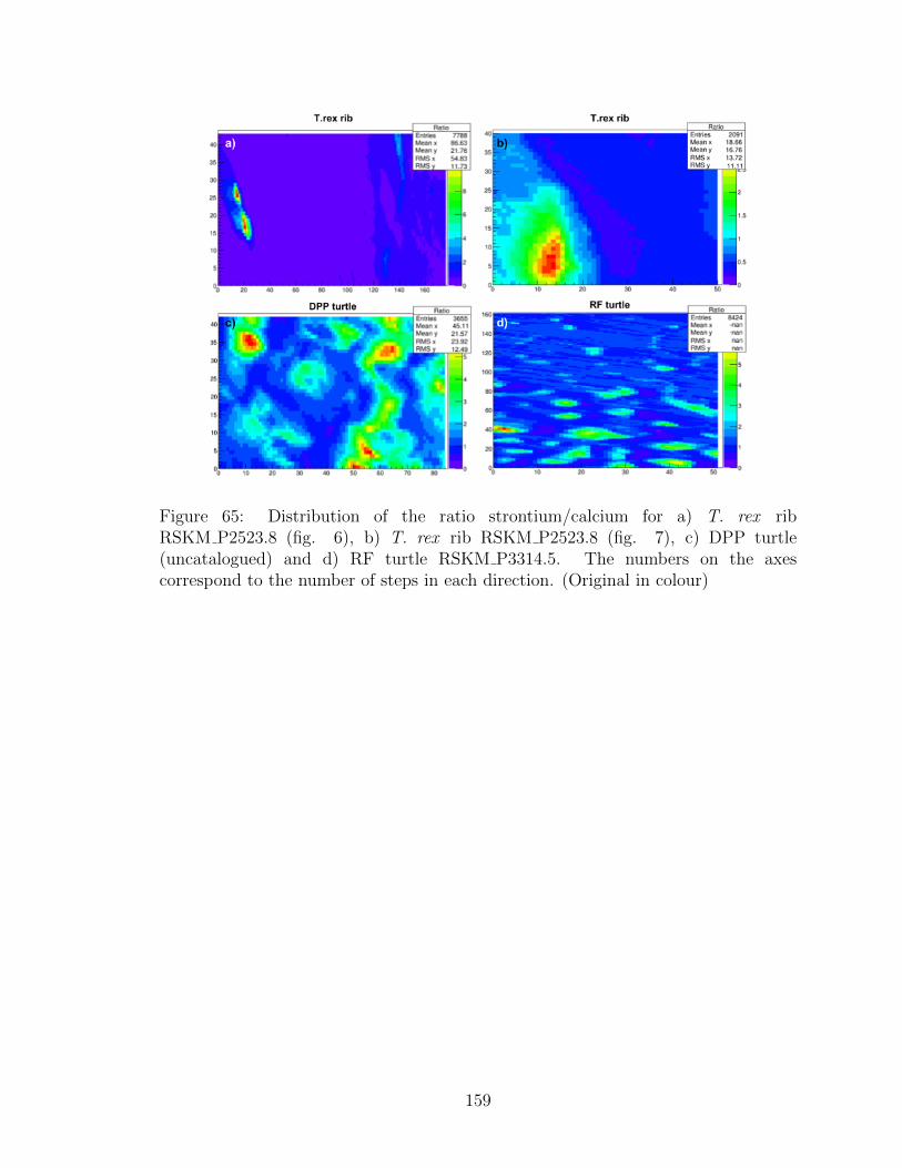
Figure 65: Distribution of the ratio strontium/calcium for a) T. rex ribRSKM P2523.8 (fig. 6), b) T. rex rib RSKM P2523.8 (fig. 7), c) DPP turtle(uncatalogued) and d) RF turtle RSKM P3314.5. The numbers on the axescorrespond to the number of steps in each direction. (Original in colour)
159

Figure 66: Distribution of the ratio yttrium/calcium for a) T. rex rib RSKM P2523.8(fig. 6), b) T. rex rib RSKM P2523.8 (fig. 7), c) DPP turtle (uncatalogued) and d)RF turtle RSKM P3314.5. The numbers on the axes correspond to the number ofsteps in each direction. (Original in colour)
Fig. 67 and 68 show the correlation plots for calcium and iron for the dinosaur
(T. rex and hadrosaur) and turtle bones studied in chapters 4 and 6, respectively.
The correlation plots for calcium and manganese for the T. rex and hadrosaur, and
the turtle bones can be seen in fig. 69 and 70, respectively.
160

Figure 67: Scatter plots relating calcium and iron for dinosaur bones. The quantitiesare represented in arbitrary units, corresponding to the number of counts under thepeak associated to a given element, corrected for variations in the electron beamcurrent which affects the X-ray beam intensity at the synchrotron facility.
Figure 68: Scatter plots relating calcium and iron for turtle bones. The quantities arerepresented in arbitrary units, corresponding to the number of counts under the peakassociated to a given element, corrected for variations in the electron beam currentwhich affects the X-ray beam intensity at the synchrotron facility.
161
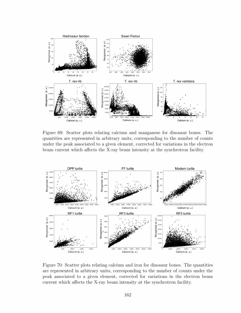
Figure 69: Scatter plots relating calcium and manganese for dinosaur bones. Thequantities are represented in arbitrary units, corresponding to the number of countsunder the peak associated to a given element, corrected for variations in the electronbeam current which affects the X-ray beam intensity at the synchrotron facility.
Figure 70: Scatter plots relating calcium and iron for dinosaur bones. The quantitiesare represented in arbitrary units, corresponding to the number of counts under thepeak associated to a given element, corrected for variations in the electron beamcurrent which affects the X-ray beam intensity at the synchrotron facility.
162

8.4 Discussion
8.4.1 Relative concentrations
The technique used to map the elemental distribution in the different types of fossils,
XRF, as used here, cannot easily generate quantitative results for the concentrations
of different elements. This is due to the use of a polychromatic beam with an unknown
spectrum and, also, due to geometric aspects of the samples used. Geometric aspects
can include, for example, the fact that bones have cavities and other irregularities
on their surface, so that the angle between the incident synchrotron radiation beam
and sample is not the same across the mapped regions. If the angle changes, so does
the beam spot size in the sample, which changes the area being probed as well as
the beam intensity per unit area. This variation makes the final image blurry and
causes a false variation in the measured concentration, respectively. The cavities in
the bone can also change the beam focus, by changing the distance between sample
and beam source. This effect is similar to what is observed when using an optical
microscope to examine a sample with an irregular surface: the focus setting that
works well for some parts of the sample causes blurry images for others, and needs
to be adjusted according to what is being visualized. Also to be considered is the
fact that differences in composition of the bones, after fossilization, may change the
depth of penetration of the incident radiation. However, some of these factors cancel
out when computing relative areas. This is because the same effects are present for
all the different chemical elements identified in each measured point on the sample.
The results in table 7 show a very large variation in the relative areas of the
elements even when the same animal is considered, as, for example, in the case when
comparing the T. rex vertebra and rib results. This is probably due to the high
influence of very local environmental conditions and the specific characteristics of
each bone. The local environmental conditions could include factors such as the
163

animal being only partially under water or buried, which could alter completely the
early taphonomic changes the fossil undergoes, even within the same piece of bone.
The changes can also be very different if a bone is broken or cracked, or between a
more dense or porous tissue. With that in mind, it becomes very difficult to interpret
such results without the knowledge of the full history of what has occurred to the
bones since the animal’s death. The large differences seen in the table above could
be explained by many different phenomena that cannot be accurately or completely
tested for (such as the ones just mentioned). Thus, the differences seen in the numbers
cannot be explained with certainty.
Some characteristics seem to be consistent between the specimens such as the
higher areas of yttrium and strontium in the turtle shell fossils when compared to
the T. rex bones. This is true even for the Frenchman Formation turtle, a specimen
coming from the same formation as the T. rex skeleton. This is indicative that the
turtle shell specimens were more readily altered than the T. rex bones, which could
be an effect of the presence of a large microbial population protecting the tissues of
the T. rex from alterations, as proposed in chapter 3. Also, the areas of iron and
manganese in the bones of most specimens are lower than those of strontium and
yttrium, probably due to association of the latter with the structure of bone apatite.
Both strontium and yttrium seem to be concentrated in the lamellae and trabeculae
(solid regions of bone) within the samples, selected for these calculations, distributed
differently from manganese and iron (usually present in higher quantities within the
osteon canals).
Although the quantitative differences between specimens is obvious (table 7), the
ratios between the areas of these elements to calcium follow a very similar qualitative
distribution in all specimens (see fig. 63 for iron). These figures show a very similar
pattern in the ratio distribution, yielding smaller ratios in the bone regions and higher
ratios inside osteons and in the sediment. The same type of pattern across different
164
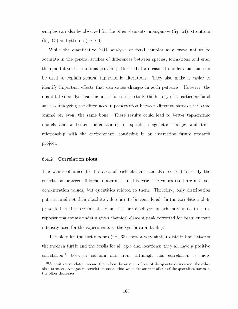
samples can also be observed for the other elements: manganese (fig. 64), strontium
(fig. 65) and yttrium (fig. 66).
While the quantitative XRF analysis of fossil samples may prove not to be
accurate in the general studies of differences between species, formations and eras,
the qualitative distributions provide patterns that are easier to understand and can
be used to explain general taphonomic alterations. They also make it easier to
identify important effects that can cause changes in such patterns. However, the
quantitative analysis can be an useful tool to study the history of a particular fossil
such as analyzing the differences in preservation between different parts of the same
animal or, even, the same bone. These results could lead to better taphonomic
models and a better understanding of specific diagenetic changes and their
relationship with the environment, consisting in an interesting future research
project.
8.4.2 Correlation plots
The values obtained for the area of each element can also be used to study the
correlation between different materials. In this case, the values used are also not
concentration values, but quantities related to them. Therefore, only distribution
patterns and not their absolute values are to be considered. In the correlation plots
presented in this section, the quantities are displayed in arbitrary units (a. u.),
representing counts under a given chemical element peak corrected for beam current
intensity used for the experiments at the synchrotron facility.
The plots for the turtle bones (fig. 68) show a very similar distribution between
the modern turtle and the fossils for all ages and locations: they all have a positive
correlation10 between calcium and iron, although this correlation is more
10A positive correlation means that when the amount of one of the quantities increase, the otheralso increases. A negative correlation means that when the amount of one of the quantities increase,the other decreases.
165
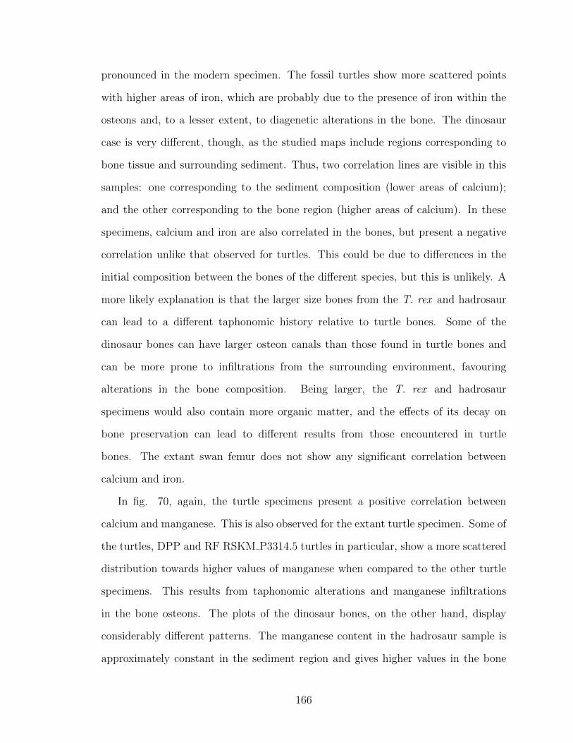
pronounced in the modern specimen. The fossil turtles show more scattered points
with higher areas of iron, which are probably due to the presence of iron within the
osteons and, to a lesser extent, to diagenetic alterations in the bone. The dinosaur
case is very different, though, as the studied maps include regions corresponding to
bone tissue and surrounding sediment. Thus, two correlation lines are visible in this
samples: one corresponding to the sediment composition (lower areas of calcium);
and the other corresponding to the bone region (higher areas of calcium). In these
specimens, calcium and iron are also correlated in the bones, but present a negative
correlation unlike that observed for turtles. This could be due to differences in the
initial composition between the bones of the different species, but this is unlikely. A
more likely explanation is that the larger size bones from the T. rex and hadrosaur
can lead to a different taphonomic history relative to turtle bones. Some of the
dinosaur bones can have larger osteon canals than those found in turtle bones and
can be more prone to infiltrations from the surrounding environment, favouring
alterations in the bone composition. Being larger, the T. rex and hadrosaur
specimens would also contain more organic matter, and the effects of its decay on
bone preservation can lead to different results from those encountered in turtle
bones. The extant swan femur does not show any significant correlation between
calcium and iron.
In fig. 70, again, the turtle specimens present a positive correlation between
calcium and manganese. This is also observed for the extant turtle specimen. Some of
the turtles, DPP and RF RSKM P3314.5 turtles in particular, show a more scattered
distribution towards higher values of manganese when compared to the other turtle
specimens. This results from taphonomic alterations and manganese infiltrations
in the bone osteons. The plots of the dinosaur bones, on the other hand, display
considerably different patterns. The manganese content in the hadrosaur sample is
approximately constant in the sediment region and gives higher values in the bone
166

area in a way that is not directly correlated to the area of calcium. In the T. rex
samples, again, two correlated distributions can be seen, one for the sediment region
and another for the bone region. However, the higher areas of manganese appear to
be associated with moderate values of calcium, which is a result of the manganese
layer found in the transition zone between bone and sediment as described in chapter
4 (section 4.5). Again, in this case, the swan femur does not show any correlation
between calcium and manganese.
Although the images are not depicted here, calcium and strontium and calcium
and yttrium appear positively correlated for all specimens of turtle and dinosaur
bones, except for the swan femur. Since these two elements seem to substitute calcium
in the bone apatite, it makes sense that where apatite is present in larger quantities
(i.e., more calcium is present), the areas of strontium and yttrium would also increase.
8.5 Conclusions
Although these plots confirm some of the observations made in the previous chapters
for specific specimens (see, for example, sections 4.4 and 6.3), a general pattern
for different animals, different formations, or different ages of fossils has not been
observed. This lack of an over-arching pattern seems to suggest that local effects
and characteristics of environment and specimens such as bone size exert a stronger
control over the final results of taphonomic alterations than the general aspects, such
as the type of animal and the stratigraphic formation of burial and preservation.
167

9 Conclusions
9.1 Summary of the findings
The work presented in this thesis represents one more step in a broader use of
synchrotron radiation and other multidisciplinary techniques in palaeontology.
Although these techniques have been used in the past, they have only recently
become more common, and there are still limited results obtained from synchrotron
radiation applications for many taxa or fossil types, such as turtles or amber
inclusions. However, the work developed here has shown that these techniques can
be very powerful to obtain chemical data that can help identify taphonomic changes
and preservation mechanisms. More than the specific results from each group of
specimens, this research has shown the potential of multidisciplinary studies of
fossils to resolve previous issues in palaeontolgy, and to extract new information
from specimens.
Some of these analyses showed a manganese layer covering T. rex bones, with
the conclusion that this layer is likely related to deposition within a fluvial
environment. They have also showed that these bones have undergone extensive
chemical changes during diagenesis, although significant preservation of bone
microstructure can still be observed. Overall, some of the results have indicated
potential preservation mechanisms for the dinosaur fossils, such as the presence of
calcium carbonates in the hadrosaur skin. This feature could be the result of early
mineralization processes that would have been key to the preservation of the
specimen involved.
I was also able to non-destructively study elemental distributions in insect
inclusions, combining these with data from synchrotron microtomography. This
method can provide a better understanding of the different types of preserved tissue
without exposing or modifying the insects, and, therefore, damaging the inclusions.
168
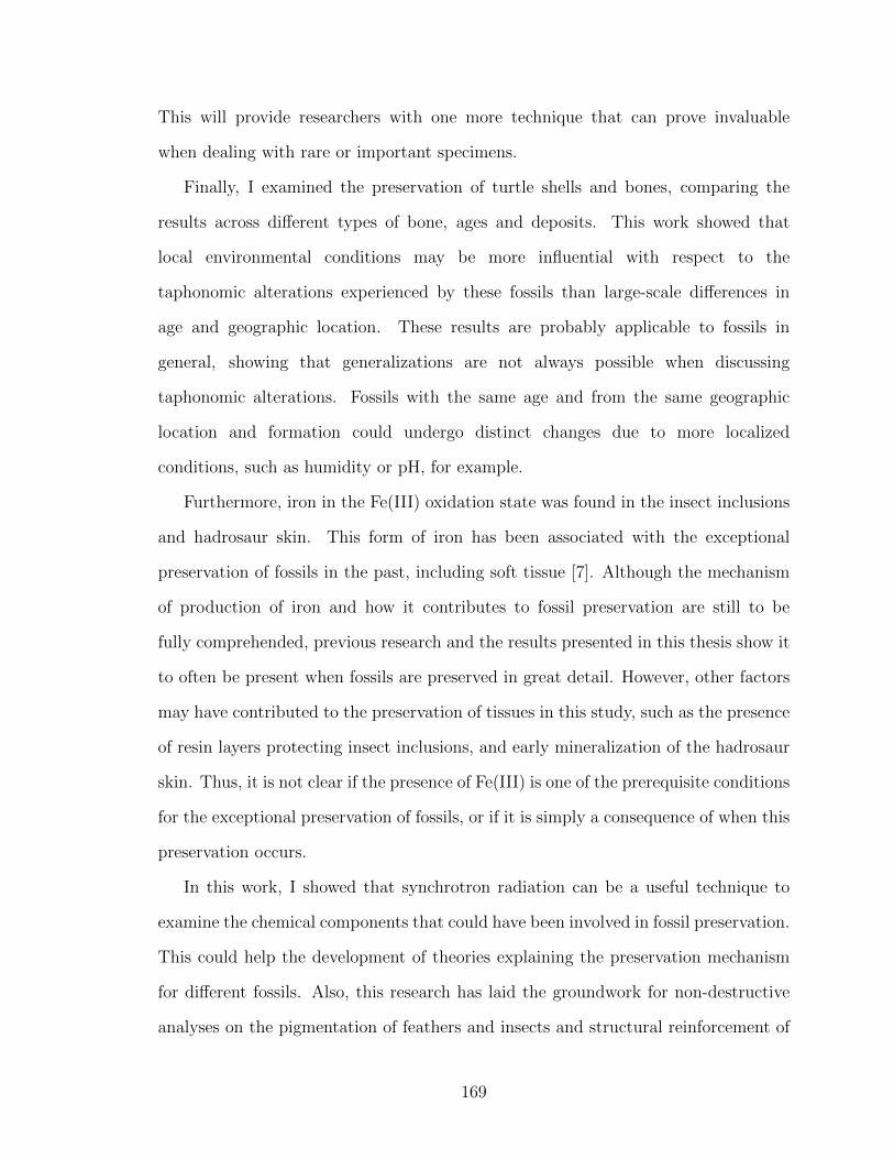
This will provide researchers with one more technique that can prove invaluable
when dealing with rare or important specimens.
Finally, I examined the preservation of turtle shells and bones, comparing the
results across different types of bone, ages and deposits. This work showed that
local environmental conditions may be more influential with respect to the
taphonomic alterations experienced by these fossils than large-scale differences in
age and geographic location. These results are probably applicable to fossils in
general, showing that generalizations are not always possible when discussing
taphonomic alterations. Fossils with the same age and from the same geographic
location and formation could undergo distinct changes due to more localized
conditions, such as humidity or pH, for example.
Furthermore, iron in the Fe(III) oxidation state was found in the insect inclusions
and hadrosaur skin. This form of iron has been associated with the exceptional
preservation of fossils in the past, including soft tissue [7]. Although the mechanism
of production of iron and how it contributes to fossil preservation are still to be
fully comprehended, previous research and the results presented in this thesis show it
to often be present when fossils are preserved in great detail. However, other factors
may have contributed to the preservation of tissues in this study, such as the presence
of resin layers protecting insect inclusions, and early mineralization of the hadrosaur
skin. Thus, it is not clear if the presence of Fe(III) is one of the prerequisite conditions
for the exceptional preservation of fossils, or if it is simply a consequence of when this
preservation occurs.
In this work, I showed that synchrotron radiation can be a useful technique to
examine the chemical components that could have been involved in fossil preservation.
This could help the development of theories explaining the preservation mechanism
for different fossils. Also, this research has laid the groundwork for non-destructive
analyses on the pigmentation of feathers and insects and structural reinforcement of
169
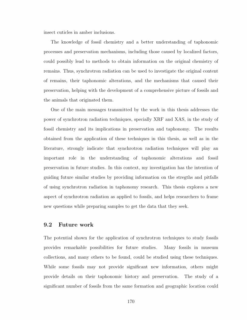
insect cuticles in amber inclusions.
The knowledge of fossil chemistry and a better understanding of taphonomic
processes and preservation mechanisms, including those caused by localized factors,
could possibly lead to methods to obtain information on the original chemistry of
remains. Thus, synchrotron radiation can be used to investigate the original content
of remains, their taphonomic alterations, and the mechanisms that caused their
preservation, helping with the development of a comprehensive picture of fossils and
the animals that originated them.
One of the main messages transmitted by the work in this thesis addresses the
power of synchrotron radiation techniques, specially XRF and XAS, in the study of
fossil chemistry and its implications in preservation and taphonomy. The results
obtained from the application of these techniques in this thesis, as well as in the
literature, strongly indicate that synchrotron radiation techniques will play an
important role in the understanding of taphonomic alterations and fossil
preservation in future studies. In this context, my investigation has the intention of
guiding future similar studies by providing information on the stregths and pitfalls
of using synchrotron radiation in taphonomy research. This thesis explores a new
aspect of synchrotron radiation as applied to fossils, and helps researchers to frame
new questions while preparing samples to get the data that they seek.
9.2 Future work
The potential shown for the application of synchrotron techniques to study fossils
provides remarkable possibilities for future studies. Many fossils in museum
collections, and many others to be found, could be studied using these techniques.
While some fossils may not provide significant new information, others might
provide details on their taphonomic history and preservation. The study of a
significant number of fossils from the same formation and geographic location could
170

also be used to better understand environmental factors associated with their
taphonomy, and how these factors affect different specimens variably. Ultimately,
detailed chemical data from fossils from several different formations could be used
to “fingerprint” a specific location in world, as has been done Mongolia [268]. This
could be done with the construction of a large database identifying the
characteristics of each location (or formation), which then could be compared to the
chemical results from an unknown fossil. Not only could this be a tool for
identifying specimens in museums of unknown origin, it could also be used to
prevent poachers from selling fossils from location where this practice is illegal. An
algorithm, such as likelihood function, could be developed to match the chemical
signature of a fossil to that of a certain location listed in the database.
For the work presented in this thesis, the next logical steps on the research into
T. rex bones would likely involve measurements of chemical standards and other
sediment pieces, to identify the state of the elements measured using XAFS. It would
also be interesting to map bones from other parts of the body of the animal to
investigate if manganese coating is also present elsewhere (or in the whole specimen).
Assuming that manganese was deposited due to the fluvial environment surrounding
the bones, measuring this layer in different parts of the dinosaur body could tell if
the whole animal was submerged or only some parts of it were.
For the insect inclusions, the next steps would include measurements of other
insect types in Baltic amber to explore if the observed preservation of soft tissues is
peculiar to certain taxon. The chemical mapping could also be used to identify
elements that characterize specific structures in insects. Together with a
three-dimensional imaging technique, this could be used to study the preservation of
determined structures in the insects. These techniques could also be used for
dedicated studies of amber types could be performed to verify how important
specific resin properties are in specimen preservation. Another possible application
171

could be examining vertebrate amber inclusions that do not present an exposed
surface, applying the same strategies used here for insects to bones and soft tissues.
In the case of the turtle shells, the measurement of the composition of the
sedimentary matrix could be used to possibly explain the origin of the differences in
the chemistry of fossils from the same formation. Variations in the surrounding
environment could have led to different availability of minerals during their
mineralization and diagenesis. The study of the sediments could also provide
information on environment at the time the remains were deposited (i.e., fluvial,
marine, or terrestrial, among others). This could also lead to explanations of those
differences related to depositional environments and a better understanding of the
fossils’ taphonomy.
For the hadrosaur skin, one of the next steps would be to accurately identify all
the chemical states of the elements detected in the sample that could not be identified
in this research. This would require the measurement of standards and comparative
samples. It would also be very useful to develop micro-tomography images of the skin
area and associate it with the chemical map, as was done for the insect inclusions.
With these results, I would be able to better determine what was preserved, and
maybe identify the structures from which the preserved carbon originated. To help
with this, other techniques could also be used, such as mass spectroscopy.
Although this work has shown that the generalization of taphonomic alterations
is not always easy (or even possible) even for fossil from the same formation and
geographic area, a deeper understanding on how local characteristics of the deposits
alter fossil chemistry could be obtained. This could be used to better understand
the history of the remains and perhaps allow for more information on their original
chemistry. One of the possible applications of this knowledge would be the
investigation of animals’ diet habits using strontium/calcium ratios, for example.
172

References
[1] Schroeter E. R., DeHart C. J., Cleland T. P., Zheng W., Thomas P. M., Kelleher
N. L., Bern M., Schweitzer M. H. 2017. Expansion for the Brachylophosaurus
canadensis Collagen I Sequence and Additional Evidence of the Preservation of
Cretaceous Protein. J. Proteome Res. 16 (2):920–932
[2] Organ, C. L., Schweitzer, M. H., Zheng, W., Freimark, L. M., Cantley, L. C.,
Asara, J. M. 2008. Molecular Phylogenetics of Mastodon and Tyrannosaurus
rex. Science 320: 499–499.
[3] Pawlicki, R., Nowogrodzka·Zagoiska, M. 1998. Blood. vessels and red blood cells
preserved in dinosaur bones. Ann Anat 180:73-77.
[4] Clarke, J. A., Ksepka, D. T., Salas-Gismondi, R., Altamirano, A. J., Shawkey,
M. D., D’Alba, L., Vinther, J., DeVries, T. J., Baby, P. 2010. Fossil Evidence for
Evolution of the Shape and Color of Penguin Feathers. Science 330 (6006):954-
957.
[5] Carney, R. M., Vinther, J., Shawkey, M. D., D’Alba, L., Ackermann, J. 2012.
New evidence on the colour and nature of the isolated Archaeopteryx feather.
Nature Communications 3:637.
[6] Martin, R. E. Taphonomy: A Process Approach. Cambridge Paleobiology Series
4. Cambridge University Press, 1999.
[7] Schweitzer, M. H., Zheng, W., Cleland, T. P., Goodwin, M. B., Boatman, E.,
Theil, E., Marcus, M. A., Fakra, S. C. 2014. A role for iron and oxygen chemistry
in preserving soft tissues, cells and molecules from deep time. Proc. R. Soc. B
281:20132741.
173

[8] Efremov, I. 1940. Taphonomy: new branch of paleontology. Pan-American
Geologist 74: 81–93.
[9] Behrensmeyer, A. K., Kidwell, S. M. 1985. Taphonomy’s Contributions to
Paleobiology. Paleobiology 11:105-119.
[10] Behrensmeyer, A. K., Kidwell, S. M., Gastaldo, R. A. 2000. Taphonomy and
paleobiology. Paleobiology 26: 103–147.
[11] Weigelt, J. 1989. Recent Vertebrate Carcasses and Their Paleobiological
Implications. University of Chicago Press.
[12] Toots, H. 1965. Sequence of disarticulation in mammalian skeletons. University
of Wyoming Contributions to Geology 4:37-39.
[13] Hill, A., Behrensmeyer, A. K. 1984. Disarticulation patterns of some modern
East African mammals. Paleobiology, 10(3): 366–376.
[14] Behrensmeier A. K. 1978. Taphonomic and ecologic information from bone
weathering. Paleobiology 4(2):150-162.
[15] Wilson, M. V. 1988. Paleoscene# 9. Taphonomic processes: information loss
and information gain. Geoscience Canada 15(2).
[16] Nussenzveig H. M. Curso de Fısica Basica - Fluidos, Oscilacoes e Ondas de
Calor. Vol. 2. 4ª Edicao. Blucher, 2008.
[17] Newton, I. 1687. Philosophiae naturalis principia mathematica. Londini, Jussu
Societatis Regiæ ac Typis Josephi Streater. Prostat apud plures Bibliopolas.
[18] Reynolds O. 1883. An Experiemental Investigation of the Circumstances Which
Determine Whether the Motion of Water Shall Be Direct or Sinuous, and of the
Law of Resistance in Parallel Channels. Phil. Trans. R. Soc. Lond. 174:935-982.
174

[19] Voorhies, MR. 1969. Taphonomy and population dynamics of an early
Pliocene vertebrate fauna, Knox County, Nebraska. University of Wyoming
Contributions to Geology Special Paper 1:1-69.
[20] Behrensmeyer AK. 1975. The taphonomy and paleoecology of Plio-Pleistocene
vertebrate assemblages east of Lake Rudolf, Kenya. Bulletin of the Museum of
Comparative Zoology 146:473-578.
[21] Hanson CB. 1980. Fluvial taphonomic processes: models and experiments. In:
Behrensmeyer AK, Hill AP (eds.) Fossils in the Making: Vertebrate Taphonomy
and Paleoecology. University of Chicago Press.
[22] Coard R. 1999. One Bone, Two Bones, Wet Bones, Dry Bones: Transport
Potentials Under Experimental Conditions. Journal of Archaeological Science
26:1369-1375.
[23] Dodson P. 1971. Sedimentology and Taphonomy of the Oldman Formation
(Campanian), Dinosaur Provincial Park, Alberta (Canada). Palaeogeography,
Palaeoclimatol., Palaeoecol. 10:21-74.
[24] Peterson JE, Bigalke, CL. 2013. Hydrodynamic Behaviours of
Pachycephalosaurid Domes in Controlled Fluvial Settings: a Case Study
in Experimenral Dinosaur Taphonomy. PALAIOS 28:285-292.
[25] Behrensmeyer, A. K. 1982. Time resolution in fluvial vertebrate assemblages.
Paleobiology 8(3): 211–227.
[26] Aquino, T., Roche, K. R., Aubenaeau, A., Packman, A. I., Bolster, D. 2017.
A Process-Based Model for Bioturbation-Induced Mixing. Scientific Reports 7:
14287.
175

[27] Guinasso NL, Jr., Schink DR. 1975. Quantitative Estimates of Biological Mixing
Rates in Abyssal Sediments. Journal of Geophysical Research 80 (21):3032-3043.
[28] Canfield DE, Raiswell R. 1991. Pyrite formation and fossil preservation. In:
Allison PA, Briggs DEG (eds.) Taphonomy: Releasing the Data Locked in the
Fossil Record, pp. 338-387. New York: Plenum Press.
[29] Briggs DEG. 2003. The Role of Decay and Mineralization in the Preservation
of Soft-Bodied Fossils. Annu. Rev. Earth Planet. Sci. 31:275-301.
[30] Schubert JK, Kidder DL, Erwin DH. 1997. Silica-replaced fossils through the
Phanerozoic. Geology 25, 11:1031-1034.
[31] Kidder, D. L., & Erwin, D. H. 2001. Secular distribution of biogenic silica
through the Phanerozoic: comparison of silica-replaced fossils and bedded cherts
at the series level. The Journal of Geology 109(4): 509–522.
[32] Channing A, Schweitzer, MH, Horner JR, McEneaney T. 2005. A silicified bird
from Quaternary hot spring deposits. Proc. R. Soc. B 272:905-911.
[33] Dettmann, M. E., Molnar, R. E., Douglas, J. G., Burger, D., Fielding, C.,
Clifford, H. T., Francis, J., Jell, P., Rich, T., Wade, M., Rich, P. V., Pledge,
N., Kemp, A., Rozefelds, A. 1992. Australian Cretaceous terrestrial faunas and
floras: biostratigraphic and biogeographic implications. Cretaceous Research 13:
207-262.
[34] Molnar, R. E. 2011. Sauropod (Saurischia: Dinosauria) material from the Early
Cretaceous Griman Creek Formation of the Surat Basin, Queensland, Australia.
Alcheringa: An Australasian Journal of Palaeontology 35(2): 303-307
[35] Hamilton-bruce, R. J., Kear, B. P. 2010. A possible succineid land snail from
the Lower Cretaceous non-marine deposits of the Griman Creek Formation at
176

Lightning Ridge, New South Wales. Alcheringa: An Australasian Journal of
Palaeontology 34(3): 325–331.
[36] Archer, M., Flannery, T. F., Molnar, R. E. 1985. First Mesozoic mammal from
Australia—an early Cretaceous monotreme. Nature 318: 363–366.
[37] Raiswell R. 1997. A geochemical framework for the application of stable sulphur
isotopes to fossil pyritization. Journal of the Geological Society 154:343-356.
[38] Xiao, S., Schiffbauer, J. D., McFadden, K. A., & Hunter, J. 2010.
Petrographic and SIMS pyrite sulfur isotope analyses of Ediacaran chert
nodules: Implications for microbial processes in pyrite rim formation,
silicification, and exceptional fossil preservation. Earth and Planetary Science
Letters,297(3-4): 481–495.
[39] Briggs DEG, Kear AJ, Martill DM, Wilby PR. 1993. Phosphatization of soft-
tissue in experiments and fossils. Journal of the Geological Society of London
150:1035-1038.
[40] Wilby PR, Whyte MA. 1995. Phosphatized soft tissues in bivalves from the
Portland Roach of Dorset (Upper Jurassic). Geol. Mag. 132:117-120.
[41] Denys C. 2001. Bones. In: Briggs DEG, Crowther PR (eds.) Paleobiology II.
Blackwell Publishing.
[42] Dauphin, T., Denys, C. and Kowalski, K. 1997. Analysis of rodent remains
accumulations: role of the chemical composition of skeletal elements. Neues
Jahrbuch fur Geologie und Palaontologie Abhandlungen 203: 295–315.
[43] Andrews, P. 1990. Owls, caves and fossils. Natural History Museum
Publications, London.
177

[44] Parker R. B., Toots H. 1980. Trace Elements in Bones as Paleobiological
Indicators. In. Behrensmeyer AK, Hill AP (eds.) Fossils in the Making:
Vertebrate Taphonomy and Paleoecology. University of Chicago Press.
[45] Avci R, Schweitzer M. H., Boyd R. D., Wittmeyer J. L., Teran Arce F, Calvo
J. O. 2005. Preservation of Bone Collagen from the Late Cretaceous Period
Studied by Immunological Techniques and Atomic Force Microscopy. Langmuir
21(8):3584-90.
[46] Collins M. J., Gernaey A. M. 2001. Proteins. In: Briggs DEG, Crowther PR
(eds.) Paleobiology II. Blackwell Publishing.
[47] Buckley, M., Warwood, S., van Dongen, B., Kitchener, A. C., Manning, P. L.
2017. A fossil protein chimera; difficulties in discriminating dinosaur peptide
sequences from modern cross-contamination. Proc. R. Soc. B 284: 20170544.
[48] Pawlicki R, Korbel A, Kubiak, H. 1966. Cells, Collagen Fibrils and Vessels in
Dinosaur Bone. Nature 211:655-657.
[49] Butterfield, N. J. 2003. Exceptional fossil preservation and the Cambrian
explosion. Integr. Comp. Biol. 43: 166–177.
[50] Bell, P. R. 2014. A Review of Hadrosaurid Skin Impressions. In Eberth DA,
Evans DC (eds). Hadrosaurs, pp. 572-590. Indiana University Press.
[51] Davis, M. 2014. Census of dinosaur skin reveals lithology may not be the
most important factor in increased preservation of hadrosaurid skin. Acta
Paleontologica Polonica 59 (3): 601–605.
[52] Osborn HF. 1911. A Dinosaur Mummy. The American Museum Journal 11:7-
11.
178
[53] Lambe LM. 1914. On the fore-limb of a carnivorous dinosaur from the Belly
River Formation of Alberta, and a new genus of Ceratopsia from the same
horizon, with remarks on the integument of some Cretaceous herbivorous
dinosaurs. The Ottawa Naturalist XXVII (10):129-135.
[54] Manning, P. L., Morris, P. M., McMahon, A., Jones, E., Gize, A., Macquaker, J.
H. S., Wolff, G., Thompson, A., Marshall, J., Taylor, K. G., Lyson, T., Gaskell,
S., Reamtong, O., Sellers, W. I., van Dongen, B. E., Buckley, M., Wogelius,
R. A. 2009. Mineralized soft-tissue structure and chemistry in a mummified
hadrosaur from the Hell Creek Formation, North Dakota (USA). Proc. R. Soc.
B 276: 3429–3437.
[55] Bell, P. R., Fanti, F., Currie, P. J., Arbour, V. M. 2014. A Mummified Duck-
Billed Dinosaur with a Soft-Tissue Cock’s Comb. Current Biology 24: 70–75.
[56] Brown, C. M., Henderson, D. M., Vinther, J., Fletcher, I., Sistiaga, A., Herrera,
J., Summons, R. E. 2017. An Exceptionally Preserved Three-Dimensional
Armored Dinosaur Reveals Insights into Coloration and Cretaceous Predator-
Prey Dynamics. Current Biology 27: 2514–2521.
[57] Barrett, P. M., Evans, D. C., Campione, N. E. 2015. Evolution of dinosaur
epidermal structures. Biol. Lett. 11: 20150229.
[58] Persons IV, W. S., Currie, P. J. 2015. Bristles before down: A new perspective
on the functional origin of feathers. Evolution (69-4):857–862.
[59] Ji, Q., Ji, S. A. 1996. On the Discovery of the earliest fossil bird in
China (Sinosauropteryx gen. nov.) and the origin of birds. Chinese Geology
(233):30–33.
[60] Chen P-j, Dong Z-m, Zhen S-n. 1998. An exceptionally well-preserved theropod
dinosaur from the Yixian Formation of China. Nature 391:147-152.
179

[61] Xu X, Zhou Z, Dudley R, Macken S, Chuong CM, Erickson GM, Varricchio
DJ. 2014. An integrative approach to understanding bird origins. Science 346
(6215):1341-1253293-10.
[62] Persons IV, W. S., Currie, P. J. 2015. Bristles before down: A new perspective
on the functional origin of feathers. Evolution 69(4): 857–862.
[63] Zheng, X. T., You, H. L., Xu, X., Dong, Z. M. 2009. An Early Cretaceous
heterodontosaurid dinosaur with filamentous integumentary structures. Nature
458: 333–336.
[64] Mayr, G., Peters, D. S., Plodowski, G., Vogel, O. 2002. Bristle-like
integumentary structures at the tail of the horned dinosaur Psittacosaurus.
Naturwissenschaften 89: 361–365
[65] Xu, X., Zhou, Z., Prum, R. O. 2001. Branched integumental structures in
Sinornithosaurus and the origin of feathers. Nature 410: 200–204.
[66] Hu, D., Hou, L., Zhang, L., Xu, X. 2009. A pre-Archaeopteryx troodontid
theropod from China with long feathers on the metatarsus. Nature 461:
640–643.
[67] Zhang F. C., Zhou Z. H., Xu X., Wang, X., Sullivan, C. 2008. A bizarre
Jurassic maniraptoran from China with elongate ribbon-like feathers. Nature
455: 1105–1108.
[68] Ji, Q., Currie, P. J., Norell, M. A., Ji, S. A. 1998. Two feathered dinosaurs from
northeastern China. Nature 393: 753–761.
[69] Xu, X., Zhou, Z., Wang, X., Kuang, X., Zhang, F., Du, X. 2003. Four-winged
dinosaurs from China. Nature 421: 335–340
180
[70] Xu, X., Guo, Y. 2009. The origin and early evolution of feathers: insights
from recent paleontological and neontological data. Vertebrata PalAsiatica 10:
311–329.
[71] Davis, P. G., Briggs, D. E. G. 1995. Fossilization of feathers. Geology 23(9):
783–786.
[72] Vinther, J., Briggs, D. E. G., Prum, R. O., Saranathan, V. 2008. The colour of
fossil feathers. Biol. Lett. 4: 522–525.
[73] Vinther, J. 2015. A guide to the field of palaeo colour. Bioessays 37: 643–656.
[74] Moyer, A. E., Zheng, W., Johnson, E. A., Lamanna, M. C., Li, D., Lacovara, K.
J., Schweitzer, M. H. 2014. Melanosomes or Microbes: Testing an Alternative
Hypothesis for the Origin of Microbodies in Fossil Feathers. Scientific Reports
4: 4233.
[75] Lindgren, J., Moyer, A., Schweitzer, M. H., Sjovall, P., Uvdal, P., Nilsson, D.
E., Heimdal, J., Engdahl, A., Gren, J. A., Schultz, B. P., Kear, B. P. 2015.
Interpreting melanin-based coloration through deep time: a critical review.
Proc. R. Soc. B 282: 20150614.
[76] Schweitzer, M. H., Lindgren, J., Moyer, A. E. 2015. Melanosomes
and ancient coloration re-examined: A response to Vinther 2015 (DOI
10.1002/bies.201500018). Bioessays 37(11): 1174–1183.
[77] McNamara M. E., Briggs, D. E. G., Orr, P. J., Field, D. J., Wang, Z. 2013.
Experimental maturation of feathers: implications for reconstructions of fossil
feather colour. Biology Letters 9(3): 20130184.
[78] Vinther, J. 2015. Fossil melanosomes or bacteria? A wealth of findings favours
melanosomes. Bioessays 38(3): 220–225.
181

[79] Labandeira CC, Beall BS, Hueber FM. 1988. Early Insect Diversification:
Evidence from a Lower Devonian Bristletail from Quebec. Science 242:913-916.
[80] Martınez-Delclos X, Briggs DEG, Penalver E. 2004. Taphonomy of insects
in carbonates and amber. Palaeogeography, Palaeoclimatology, Palaeoecology
203:19-64.
[81] Grimaldi, D., Engel, M. S. 2005. Evolution of Insects. Cambridge University
Press, 755 pages.
[82] Poinar, G.O. Jr., 1992. Life in Amber. Stanford University Press, Stanford, 350
pp.
[83] Anderson, K. B., Crelling, J. C. 1995. Introduction. In: Anderson, K.G.,
Crelling, J.C., (Eds.), Amber, Resinite and Fossil Resins. American Chemical
Society Symposium Series 617, Washington, DC, pp. 11–17.
[84] Beck, C.W. 1999. The Chemistry of Amber. Estudios Museo Ciencias Naturales
de Alava 14 (2): 33–48.
[85] Kosmowska-Ceranowicz, B. 1999. Succinite and some other fossil resins in
Poland and Europe (Deposits, finds, features and differences in IRS). Estudios
Museo Ciencias Naturales de Alava 14 (2): 73–117.
[86] van Bergen, P. F., Collinson, M. E., Scott, A. C., de Leeuw, J. W. 1995.
Unusual resin chemistry from Upper Carboniferous pteridosperm resin rodlets.
In: Anderson, K.G., Crelling, J.C. (Eds.), Amber, Resinite and Fossil Resins.
American Chemical Society Symposium Series 617, Washington, DC, pp.
149–169.
[87] Langenheim, J. H. 1995. Biology of amber-producing trees: Focus on case
studies of Hymenaea and Agathis. In: Anderson, K.G., Crelling, J.C. (Eds.),
182

Amber, Resinite and Fossil Resins. American Chemical Society Symposium
Series 617, Washington, DC, pp. 1–31.
[88] True, R. P., Snow, A. G., 1949. Gum flow from turpentine pines inoculated
with the pitch-canker Fusarium. J. For. 47: 894–899.
[89] Farrell, B. D., Dussourd, D. E., Mitter, C. 1991. Escalation of plant defense:
Do latex/resin canals spur plant diversification? Am. Nat. 138: 881–900.
[90] Henwood, A., 1992. Insect Taphonomy from Tertiary Amber of the Dominican
Republic. Ph.D. Thesis, University of Cambridge, 166 pp.
[91] Henwood A. 1993. Recent plant resins and the taphonomy of organisms in
amber: A review. Mod. Geol. 19: 35-59.
[92] Dell, B., McComb, A. B. 1978. Plant resins – their formation, secretion and
possible functions. Adv. Bot. Res. 6: 275–316.
[93] Langenheim, J. H. 1994. Higher plant terpenoids: A phytocentric overview of
their ecological roles. J. Chem. Ecol. 20: 1223–1280.
[94] Poinar, G.O. Jr., Poinar, R. 1999. The Amber Forest: A Reconstruction of a
Vanished World. Princeton University Press, 239 pp.
[95] Koteja, J. 1996. Syninclusions. Inclusion–Wrostek 22: 10–12.
[96] Langenheim, J. H. 1995. Biology of amber-producing trees: Focus on case
studies of Hymenaea and Agathis. In: Anderson, K.G., Crelling, J.C. (Eds.),
Amber, Resinite and Fossil Resins. American Chemical Society Symposium
Series 617, Washington, DC, pp. 1–31.
[97] Alencar, J.C. 1982. Estudos silviculturais de uma populacao natural de
Copaifera multijuga Hayne – Leguminosae, na Amazonia Central. 2 – Producao
de oleoresina. Acta Amazonica 12: 75–89.
183

[98] Hillis, W. E. 1987. Heartwood and Tree Exudates. Springer.
[99] Wagensberg, J., Brandao, C. R. F., Baroni-Urbani, C. 1996. Le mystere de la
chambre jaune. Recherche 288: 54–59.
[100] Grimaldi, D. A. 1996. Amber: window to the past. Harry N. Abrams,
Publishers, in association with the American Museum of Natural History.
[101] Poinar, G. O. 1992. Life in amber. Stanford University Press.
[102] Grimaldi, D., Shedrinsky, A., Wampler, T. P. 2000. A remarkable deposit
of fossiliferous amber from the Upper Cretaceous (Turonian) of New Jersey.
Studies on fossils in amber, with particular reference to the Cretaceous of New
Jersey, 1, 76.
[103] Briggs, D. E., Crowther, P. R. (Eds.). 2008. Palaeobiology II. John Wiley &
Sons.
[104] Grimaldi, D., Bonwich, E., Delannoy, M., Doberstein, S. 1994. Electron
Microscopic Studies of Mummified Tissues in Amber Fossils. In American
Museum Novitates, Number 3097. American Museum of Natural History, 31
pages.
[105] Allison, P. A., Briggs, D. E. G. 1991. The taphonomy of softbodied animals. In:
Donovan, S.K. (Ed.), The Processes of Fossilization. Belhaven Press, London,
pp. 120–140.
[106] Henwood, A. 1992. Exceptional preservation of dipteran flight muscle and the
taphonomy of insects in amber. Palaios 7: 203–212.
[107] Stankiewicz, B. A., Poinar, H. N., Briggs, D. E. G., Evershed, R. P., Poinar,
G. O., Jr. 1998. Chemical preservation of plants and insects in natural resins.
Proc. R. Soc. Lond. B 265:641-647.
184
[108] Poinar, G. O., Jr. 1991. Resinites, with examples from New Zealand and
Australia. Fuel Proc. Technol. 28: 135–148.
[109] Zherikhin, V. V., Eskov, K. Y. 1999. Mesozoic and Lower Tertiary Resins in
Former USSR. Estudios del Museo de Ciencias Naturales de Alava 14 (spec. no.
2): 119–131.
[110] Seilacher, A. 1970. Begriff und Bedeutung der Fossil-Lagerstatten. Neues
Jahrbuch fur Geologie und Palaontologie, Monatshefte 1970:34–39.
[111] Seilacher, A. 1990. Taphonomy of Fossil-Lagerstatten. In Briggs DEK, Crowther
PR (eds.) Palaeobiology: a Synthesis. Blackwell, pp. 266–270.
[112] Allison PA. 1988. Konservat-Lagerstatten: cause and classification. Paleobiology
14(4):331-344.
[113] Veksler, V. I. 1944. A new method of accelerating relativistic particles. Comptes
Rendus (Dokaldy) de l’Academie Sciences de l’URSS 43(8): 329–331.
[114] McMillan, E. M. 1945. The Synchrotron - A Proposed High Energy Particle
Accelerator. Phys. Rev. 68:143.
[115] Salsig Jr., W. W. 1949. First Large Synchrotron Placed in Operation.
United States Atomic Energy Commission. University of California Radiation
Laboratory.
[116] Mobilio, S., Boscherini, F., Meneghini, C. 2015. Synchrotron Radiation: Basics,
Methods and Applications. Springer-Verlag Berlin Heidelberg.
[117] Winick, H. 1997. Fourth Generation Light Sources. 1997 Particle
Accelerator Conference Proceedings, Vancouver. Available at:
http://accelconf.web.cern.ch/AccelConf/pac97/papers/pdf/FBC003.PDF
(accessed on September/2016).
185

[118] Canadian Light Source. Inside the Synchrotron. Available at
http://www.lightsource.ca/pages/inside the synchrotron (accessed on
October/2016).
[119] Wiedemann, H. 2007. Particle Accelerator Physics. Springer-Verlag Berlin
Heidelberg.
[120] Sundaresan, M. K. 2001. Handbook of Particle Physics. CRC Press.
[121] Jackson, J. D. 1999. Classical Electrodynamics. Third Edition. John Wiley &
Sons.
[122] Shackley, M. S. 2011. X-Ray Fluorescence Spectrometry (XRF) in
Geoarchaeology. Springer-Verlag New York.
[123] Haschke, M. 2014. Laboratory Micro-X-Ray Fluorescence Spectroscopy:
Instrumentation and Applications. Springer.
[124] Yano, J., Yachandra, V. K. 2009. X-ray absorption spectroscopy. Photosynth
Res 102:241-254.
[125] Cabaret, D. et al. 2010. First-principles calculations of X-ray absorption spectra
at the K-edge of ed transition metals: an electronic structure analysis of the
pre-edge. Phys. Chem. Chem. Phys. 12:5619-5633.
[126] Benfatto, M., Congiu-Castellano, A., Daniele, A., Della Longa, S. 2001. MXAN:
a new software procedure to perform geometrical fitting of experiemental
XANES spectra. J. Synchrotron Rad. 8:267-269.
[127] CERN. Minuit. Available at: https://seal.web.cern.ch/seal/snapshot/work-
packages/mathlibs/minuit/ (ccessedetailsd on November/2016).
186
[128] Ravel, B., Newville, M. 2005. ATHENA, ARTMEIS, HEPHAESTUS: data
analysis for X-ray absorption spectroscopy using IFEFFIT. J. Synchrotron Rad.
12:537-541.
[129] Rehr, J. J. et al. 2010. Parameter-free calculations of X-ray spectra with FEFF9.
Phys. Chem. Chem. Phys. 12:5503-5513
[130] Winick, H., Brown G., Halbach, K., Harris, J. 1981. Wiggler and Undulator
Magnets. Physics Today, 34, 5, p. 50-63.
[131] Hofman, A., et al. 1967. Design and Performance of the Damping System
for Beam Storage in the Cambridge Electron Accelerator. Proceeedings
6th International Conference on High Energy Accelerators CEAL-2000,
p.123.studies
[132] Photon Science - DESY. What is SR, how is it generated
and are its properties? Available at http://photon-
science.desy.de/research/studentsteaching/primers/synchrotron radiation/index eng.html
(accessed on September/2016).
[133] Ginzberg, V. L. 1947. Izv. Akad nauk. SSSR, Ser. Fiz., II, 165.
[134] Motz, H., Thon, W., Whitehurst, R. N. 1953. Experiments on Radiation by
Fast Electron Beams. Journal of Applied Physics 24, 7:826.
[135] Als-Nielsen, J., McMorrow, D. 2001. Elements of Modern X-ray Physics. John
Wiley & Sons Ltd.
[136] Moller, K. D. 1988. Optics. University Science Book.
[137] Duller, G. et al. A High Precision, High Stability, Four
Bounce Monochromator for Diamond Beamline I20. Available at:
187

https://medsi.lbl.gov/SysIncludes/retrieve.php?url=https://medsi.lbl.gov/files/page 137/Presentations Papers/High Precision Positioning Mechanisms/A High Precision High Stability Four-
Bounce X-ray Monochromator for Diamond Beamline I20 - G. Duller -
PAPER.pdf (accessed on October, 2016).
[138] Bunker, G. 2010. Introduction to XAFS. Cambridge University Press.
[139] Le, B. Q., Nurcombe, V., Cool, S. M., van Blitterswijk, C. A., de Boer, J.,
LaPointe, V. L. S. 2017. The Components of Bone and What They Can Teach
Us about Regeneration. Materials 11(1): E14.
[140] Tokaryk, T. T. 1997. A rex with a new home. Geology Today September-
October:190-193.
[141] Benton, M. J. 2012. Origin and Early Evolution of Dinosaurs. In Brett-Surman
M. K., Holtz, Jr., T. R., Farlow, J. O., (eds.) The Complete Dinosaur. Indiana
University Press, Second Edition, pp: 330-345.
[142] Holtz Jr., T. R., Brett-Surman, M.K. 2012. The Osteology of the Dinosaurs.
In Brett-Surman M. K., Holtz, Jr., T. R., Farlow, J. O., (eds.) The Complete
Dinosaur. Indiana University Press, Second Edition, pp: 134-149.
[143] Yates, A. M. 2012. Basal Sauropodomorpha: The “Prosauropods”. In Brett-
Surman M. K., Holtz, Jr., T. R., Farlow, J. O., (eds.) The Complete Dinosaur.
Indiana University Press, Second Edition, pp: 424-443.
[144] Wilson, J. A., Rogers, K. C. 2012. Sauropoda. In Brett-Surman M. K., Holtz,
Jr., T. R., Farlow, J. O., (eds.) The Complete Dinosaur. Indiana University
Press, Second Edition, pp: 444-481.
[145] Holtz Jr., T. R. 2012. Theropods. In Brett-Surman M. K., Holtz, Jr., T. R.,
Farlow, J. O., (eds.) The Complete Dinosaur. Indiana University Press, Second
Edition, pp: 346-423.
188

[146] Huttenlocker, A. K., Woodward, H. N., Hall B. K. 2013.The Biology of Bone.
In Padian, K, Lamm, E-T. (eds.) Bone Histology of Fossil Tetrapods. University
of California Press, pp:13-34.
[147] Ralston, S. H. 2017. Bone structure and metabolism. Medicine 45(9): 560–564.
[148] Schroeder, H. A., Tipton, I. H., Nason, A. P. 1972. Trace metals in man:
strontium and barium. J. Chron. Dis. 25: 491–517.
[149] Wang, Q., Xu, J., Jin, H., Zheng, W., Zhang, X., Huang, Y., Qian, Z. 2017.
Artificial periosteum in bone defect repair—A review. Chinese Chemical Letters
28(9): 1801–1807.
[150] Allen, M. R., Hock, J. M., Burr, D. B. 2004. Periosteum: biology, regulation,
and response to osteoporosis therapies. Bone 35: 1003–1012.
[151] Seeman, E. 2007. The periosteum – a surface for all seasons. Osteoporos. Int.
18: 123–128.
[152] Bergmann, U., Morton, R. W., Manning, P. L., Sellers, W. I., Farrar, S.,
Huntley, K. G., Wogelius, R. A., Larson, P. 2010. Archaeopteryx feathers and
bone chemistry fully revealed via synchroyron imaging. PNAS 107 (20):9060-
9065.
[153] Bergmann, U., Manning, P. L., Wogelius, R. A. 2012. Chemical Mapping of
Paleontological and Archeological Artifacts with Synchrotron X-Rays. Annu.
Rev. Anal. Chem. 5:361-89.
[154] Tolhurst, T., M. Barbi, and T. Tokaryk. 2015. Effective beam method for
element concentrations. Journal of Synchrotron Radiation 22: 393–399.
[155] Barbi, M., Tokaryk, T., Tolhurst, T. 2014. Synchrotron Radiation as a Tool in
Paleontology. Physics in Canada 70(1): 8–12.
189
[156] Anne, J., Edwards, N. P., Wogelius, R. A., Tumarkin-Deratzian, A. R., Sellers,
W. I., van Veelen, A., Bergmann, U., Sokaras, D., Alonso-Mori, R., Ignatyev,
K., Egerton, V. M., Manning R., L. 2014. Synchrotron imaging reveals bone
healing and remodelling strategies in extinct and extant vertebrates. J. R. Soc.
Interface 11:20140277.
[157] Dumont, M., Zoeger, N., Streli, C., Wobrauschek, P., Falkenberg, G., Sander,
P. M., Pyzalla, A. R. 2009. Synchrotron XRF Analyses of Element Distribution
in Fossilized Sauropod Dinosaur Bones. Internacional Centre for Diffraction
Data, Denver X-ray Conference (DXC) on Applications of X ray Analysis.
[158] Zougrou, I. M., Katsikini, M., Pinakidou, F., Paloura, E. C., Papadopoulou,
L., Tsoukala, E. 2013. Study of fossil bones by synchrotron radiation micro-
spectroscopic techniques and scanning electron microscopy. J. Synchrotron Rad.
21: 149–160.
[159] Brunetti, A., Piga, G., Lasio, B., Golosio, B., Oliva, P., Stegel, G., Enzo, S.
2013. Elemental investigation on Spanish dinosaur bones by x-ray fluorescence.
Physica Scripta 88(1): 015802.
[160] Brown, C. M., Boyd, C. A., Russell Fls, A. P. 2011. A new basal ornithopod
dinosaur (Frenchman Formation, Saskatchewan, Canada), and implications for
late Maastrichtian ornithischian diversity in North America. Zoological Journal
of the Linnean Society 163: 1157-1198.
[161] McIver, E. E. 2002. The paleoenvironment of Tyrannosaurus rex from
southwestern Saskatchewan, Canada. Can. J. Earth. Sci. 39: 207-221.
[162] Furnival, G. M. 1946. Cypress Lake Map Area, Saskatchewan. Memoir 242.
Geological Survey of Canada, Ottawa, 161 pp.
190
[163] Kupsch, W. O. 1956. Geology of eastern Cypress Hills Saskatchewan.
Saskatchewan Department of Mineral Resources. Report No. 20, 30 p.
[164] Kolaceke, A. Velez, M. I., Coulson, I. M., Barbi, M. and Tokaryk, T. 2018.
Lithostratigraphy of sections surrounding a nearly complete Tyrannosaurus
rex (“Scotty”) excavation in southwestern Saskatchewan, Canada. Manuscript
submitted for publication.
[165] Storer, J. E. 1991. The mammals of the Gryde Local Fauna, Frenchman
Formation (Maastrichtian: Lancian), Saskatchewan. Journal of Vertebrate
Paleontology 11(3): 350-369.
[166] Fraser, F. J. McLearn, F.D., Russell, L.S., Warren, P.S., Wickenden, R.T.D.,
1935. Geology of southern Saskatchewan. Geological Survey of Canada, Memoir
176: 1-137.
[167] Kupsch, W. O. 1957. Frenchman Formation of Eastern Cypress Hills,
Saskatchewan, Canada. Bulletin of the Geological Society of America 68: 413-
420.
[168] Nichols, D. J., Jarzen, D. M., Orth, C. J., Oliver, P. Q. 1986. Palynological and
iridium anomalies at cretaceous-tertiary boundary, South-central Saskatchewan.
Science 231(4739): 714-717.
[169] Lerbekmo, J. F., Sweet, A. R., Louis, R. M. St. 1987. The relationship between
the iridium anomaly and palynological floral events at three Cretaceous-Tertiary
boundary localities in western Canada. Geological Society of America Bulletin
99: 325-330.
[170] Kamo, S. L., Krogh, T. E. 1995. Chicxulub crater source for shocked zircon
crystals from the Cretaceous-Tertiary boundary layer, Saskatchewan: Evidence
from new U-Pb data. Geology 23(3): 281-284.
191

[171] Royal Saskatchewan Museum. “Scotty” The T. rex. Available at:
http://royalsaskmuseum.ca/pub/Fossil%20Video%20Contest/Trex english.pdf.
Acessed on June, 2018.
[172] Fricke, H. C., Rogers, R. R., Gates, T. A. 2009. Hadrosaurid migration:
inferences based on stable isotope comparisons among Late Cretaceous dinosaur
localities. Paleobiology 35(2): 270–288.
[173] Feng, R., Gerson, A., Ice, G., Reininger, R., Yates, B., McIntyre,
S. 2007. VESPERS: A Beamline for Combined XRF and XRD
Measurements. Synchrotron Radiation Instrumentation: Nineth International
Conference. Available at: https://www.ornl.gov/directorate/psdmst/x-
ray/pdf/pubs/2007/Feng Vespers07.pdf. Acessed on October, 2016.
[174] Hu, Y. F., Coulthard, I., Chevrier, D., Wright, G., Igarashi, R., Sitnikov, A.,
Yates, B. W., Hallin, T. K., Sham, T. K., and Reininger, R. 2010. Preliminary
commissioning and performance of the Soft X-ray Micro-characterization
Beamline at the Canadian Light Source. AIP Conference Proceedings 1234:
343–346.
[175] Sole, V. A., Papillon, E., Cotte, M., Walter, Ph., Susini, J. 2007. A
multiplatform code for the analysis of energy-dispersive X-ray fluorescence
spectra. Spectrochim. Acta Part B 62: 63-68.
[176] Ravel, B., Newville, M. 2005. ATHENA, ARTEMIS, HEPHAESTUS: data
analysis for X-ray absorption spectroscopy using IFEFFIT. Journal of
Synchrotron Radiation 12: 537–541.
[177] Newville, M. 2013. Larch: An Analysis Package for XAFS and Related
Spectroscopies. J. Phys.: Conf. Ser. (430):012007.
192
[178] Parker, R. B., Toots, H. 1980. Trace Elements in Bones as Paleobiological
Indicators. In Behrensmeyer, A. K., Hill, A. P., (eds.) Fossils in the Making:
Vertebrate Taphonomy and Paleoecology. University of Chicago Press, pp. 199.
[179] Boivin, G., Deloffre, P., Perrat, B., Panczer, G., Boudeulle, M., Mauras, Y.,
Allain, P., Tsouderos, Y., Meunier, P. J. 1996. Strontium distribution and
interactions with bone mineral in monkey iliac bone after strontium salt (S
12911) administration. J Bone Miner Res. 11(9):1302-11.
[180] Sillen, A., Sealy, J. C. 1995. Diagenesis of Strontium in Fossil Bone: A
Reconsideration of Nelson et al. (1986). Journal of Archaeological Science
22:313–320.
[181] Lopez-Gonzalez, F., Grandal-d’Anglade, A., Vidal-Romanı, J. R. 2006.
Deciphering bone depositional sequences in caves through the study of
manganese coatings. Journal of Archaeological Science 33: 707–717.
[182] Allaby, Michael (ed.). 2015. A Dictionary of Geology and Earth Sciences. Oxford
University Press (online).
[183] Muir, M. D. 1978. Microenvironments of Some Modern and Fossil Iron- and
Manganese-Oxidizing Bacteria. In Krumbein, W. E., (ed.) Environmental
Biogeochemistry and Geomicrobiology. Ann Arbor Science, vol. 3, p. 937.
[184] Potter, R. M., Rossman, G. R. 1979. Mineralogy of manganese dendrites and
coatings. American Mineralogist 64: 26–30.
[185] White, W. B. 1976. Cave minerals and speleothems. In Ford, T. D., Cullingford,
C. H. D. (Eds.), The Science of Speleology, Academic Press, London, pp.
267–327.
193
[186] Keenan, S. W., Engel, A. S., Roy, A., Bovenkamp-Langlois, G. 2015. Evaluating
the consequences of diagenesis and fossilization on bioapatite lattice structure
and composition. Chemical Geology 413:18-27.
[187] Brinza, L., Schofield, P. F., Hodson, M. E., Weller, S., Ignatyev, K., Geraki,
K., Quinn, P. D., Mosselmans, J. F. W. 2014. Combining μXANES and μXRD
mapping to analyse the heterogeneity in calcium carbonate granules excreted
by the earthworm Lumbricus terrestris. J. Synchrotron Rad. 21:235-241.
[188] Li, D., Bancroft, G. M., Kasrai, M. 1995. S K- and L-edge X-ray absorption
spectroscopy of metal sulfides and sulfates: applications in mineralogy and
geochemistry. The Canadian Mineralogist 33:949-960.
[189] Petit, P.-E., Farges, F., Wilke, M., Sole, V. A. 2001. Determination of the
iron oxidation state in Earth materials using XANES pre-edge information. J.
Synchrotron Rad. 8:952-954.
[190] Reguer, S., Mirambet, F., Remazeilles, C., Vantelon, D., Kergourlay, F., Neff,
D., Dillmann, P. 2015. Iron corrosion in archaeological context: Structural
refinement of the ferrous hydroxychloride β-Fe2(OH)3Cl. Corrosion Science
(100):589-598.
[191] Bazin, D., Dessombz, A., Nguyen, C., Ea, H. K., Liote, F., Rehr, J.,
Chappard, C., Rouziere, S., Thiaudiere, D., Reguer, S., Daudon, M. 2014. The
status of strontium in biological apatites: an XANES/EXAFS investigation. J.
Synchrotron Rad. 21:136-142.
[192] Kolaceke, A. P., McKellar, R. C., Barbi, M. 2018. A non-destructive
technique for chemical mapping of insect inclusions in amber. PalZ.
https://doi.org/10.1007/s12542-018-0412-x
194

[193] Weitschat, W., Wichard, W. 2002. Atlas of Plants and Animals in Baltic Amber.
Verlag Dr. Friedrich Pfeil.
[194] Wolfe, A. P., Tappert, R., Muehlenbachs, K., Boudreau, M., McKellar, R.
C., Basinger, J. F., Garrett, A. 2009. A new proposal concerning the botanical
origin of Baltic amber. Proceedings of the Royal Society B 276 (1672):3403-3412
[195] Weitschat, W., Wichard, W. 2010. Baltic Amber. In: Penney, D. (ed.)
Biodiversity of fossils in amber from the major world deposits. Siri Scientific
Press.
[196] Krynicki V. E. 2013. Primitive ants (Hymenoptera: Sphecomyrminae) in the
Campanian (LateCretaceous) of North Carolina (USA). Life: The Excitement
of Biology 1:156-165.
[197] Duncan, I. J., Titchener, F., Briggs, D. E. G. 2003. Decay and Disarticulation
of the Cockroach: Implications for Preservation of the Blattoids of Writhlington
(Upper Carboniferous), UK. PALAIOS 18: 256–265
[198] McCoy, V. E., Soriano, C., Gabbott, S. E. 2017. A review of preservational
variation of fossil inclusions in amber of different chemical groups. Earth and
Environmental Science Transactions of the Royal Society of Edinburgh: 1–9.
[199] McCoy, V. E., Soriano, C., Pegoraro, M., Luo, T., Boom, A., Foxman, B.,
Gabbott, S. E. 2018. Unlocking preservation bias in the amber insect fossil
record through experimental decay. decay. PLoS ONE 13(4): e0195482.
[200] Perrichot V., Lacau, S., Neraudeau, D., Nel, A. 2007. Fossil evidence for the
early ant evolution. Naturwissenschaften 95: 85–90.
[201] Barden, P., Grimaldi, D. A. 2016. Adaptive Radiation in Socially Advanced
Stem-Group Ants from the Cretaceous. Current Biology 26: 515–521.
195

[202] LaPolla J. S., Dlussky, G. M., Perrichot, V. 2013. Ants and the Fossil Record.
Annu. Rev. Entomol. 58: 609–30.
[203] Bolton, B. 1994. Identification guide to the ant genera of the world. Harvard
University Press, 222 pages.
[204] Poinar, Jr., G. O., Hess, R. 1982. Ultrastructure of 40-Million-Year-Old Insect
Tissue. Science 215: 1241–1242.
[205] Speranza, M., Wierzchos, J., Alonso, J., Bettuchi, L., Martın-Gonzalez, A.,
Ascaso, C. 2010. Traditional and new microscopy techniques applied to the
study of microscopic fungi included in amber. Microscopy: Science, Technology,
Application and Education 2: 1135–1145.
[206] McKellar, R.C., Chatterton, B. D. E., Wolfe, A. P., Currie, P. J. 2011. A diverse
assemblage of Late Cretaceous dinosaur and bird feathers from Canadian amber.
Science 333(6049): 1619–1622.
[207] Lak, M., Neraudeau, D., Nel, A., Cloetens, P., Perrichot, V., Tafforeau, P. 2008.
Phase contrast X-ray synchrotron imaging: opening access to fossil inclusions
in opaque amber. Microscopy and Microanalysis. 14: 251–259.
[208] Kirejtshuk, A.G., Azar, D., Tafforeau, P., Boistel, R., Fernandez, V. 2009. New
beetles of Polyphaga (Coleoptera, Polyphaga) from Lower Cretaceous Lebanese
amber. Denisia 26: 119–130.
[209] Soriano, C., Archer, M., Azar, D., Creaser, P., Delclos, X., Godthelp, H., Hand,
S., Jones, A., Nel, A., Neraudeau, D., Ortega-Blanco, J. 2010. Synchrotron X-
ray imaging of inclusions in amber. Comptes Rendus Palevol 9(6): 361–368.
[210] Tafforeau, P., Boistel, R., Boller, E., Bravin, A., Brunet, M., Chaimanee, Y.,
Cloetens, P., Feist, M., Hoszowska, J., Jaeger, J. J., Kay, R. F., Lazzari,
196

V., Marivaux, L., Nel, A., Nemoz, C., Thibault, X., Vignaud, P., Zabler, S.
2006. Applications of X-ray synchrotron microtomography for nondestructive
3D studies of paleontological specimens. Appl. Phys. A Mater. 83: 195–202.
[211] Riedel, A., dos Santos Rolo, T., Cecilia, A., van de Kamp, T. 2012.
Sayrevilleinae Legalov, a new subfamily of fossil weevils (Coleoptera,
Curculionoidea, Attelabidae) and the use of synchrotron microtomography to
examine inclusions in amber. Zoological Journal of the Linnean Society 165:
773-794.
[212] van de Kamp, T., dos Santos Rolo, T., Baumbach, T., Krogmann, L. 2014.
Scanning the Past – Synchrotron X-Ray Microtomography of Fossil Wasps in
Amber. Entomologie heute 26: 151–160.
[213] Henderickx, H., Tafforeau, P., Soriano, C. 2012. Phase-contrast synchrotron
microtomography reveals the morphology of a partially visible new
Pseudogarypus in Baltic amber (Pseudoscorpiones: Pseudogarypidae).
Palaeontologia Electronica 15(2): 17A.
[214] (7) Scanning the past - synchrotron X-ray microtomography
of fossil wasps in amber | Request PDF. Available from:
https://www.researchgate.net/publication/268504916 Scanning the past -
synchrotron X-ray microtomography of fossil wasps in amber [accessed Oct
20 2018].
[215] Xing, L., McKellar, R. C., Xu, X., Li, G., Bai, M., Persons IV, W. S., Miyashita,
T., Benton, M. J., Zhang, J., Wolfe, A. P., Yi, Q., Tseng, K., Ran, H., and P.J.
Currie. 2016. A feathered dinosaur tail with primitive plumage trapped in mid-
Cretaceous amber. Current Biology 26: 1–9.
197
[216] Greenwalt, D.E., Goreva, Y. S., Siljestrom, S. M., Rose, T., Harbach, R. E.
2013. Hemoglobin-derived porphyrins preserved in a Middle Eocene blood-
engorged mosquito. Proceedings of the National Academy of Sciences USA
110(1849): 18496–18500.
[217] Barling, N., Martill, D. M., Heads, S. W., Gallien, S. 2015. High fidelity
preservation of fossil insects from the Crato Formation (Lower Cretaceous) of
Brazil. Cretaceous Research 52: 605–622.
[218] Nascimbene, P., and Silverstein, H. 2000. The preparation of fragile Cretaceous
ambers for conservation and study of organismal inclusions. In Studies of fossils
in amber, with particular reference to the Cretaceous of New Jersey. Edited by
D. Grimaldi. Backhuys Publishers, Leiden, the Netherlands. pp. 93–102.
[219] McKellar, R. C., Engel, M. S. 2011. First Mesozoic Microphysidae (Hemiptera):
a new genus and species in Late Cretaceous amber from Canada. Can. Entomol.
143: 349–357.
[220] Engel, M. S., Thomas, J. C., Alqarni, A. S. 2017. A new genus of protorhyssaline
wasps in Raritan amber (Hymenoptera, Braconidae). Zookeys 711: 103–111.
[221] Brun, R., Rademakers, F. 1997. ROOT - An Object Oriented Data Analysis
Framework. Proceedings AIHENP’96 Workshop, Lausanne, Sep. 1996, Nuclear
Instruments and Methods in Physics Research A 389: 81–86. See also
http://root.cern.ch/.
[222] Wysokinski, T. W., Chapman, D., Adams, G., Renier, M., Suortti, P.,
Thomlinson W. 2015. Beamlines of the biomedical imaging and therapy facility
at the Canadian Light Source-Part 3. Nuclear Instruments and Methods in
Physics Research A 775(1): 1–4.
198

[223] Bukejs, A., Alekseev, V. I., Cooper, D. M. L., King, G. A., McKellar, R. C.
2017. Contributions to the palaeofauna of Ptinidae (Coleptera) known from
Baltic amber. Zootaxa 4344 (1): 181–188.
[224] Schneider, C. A., Rasband, W. S., Eliceiri, K. W. 2012. NIH Image to ImageJ:
25 years of image analysis. Nature methods 9(7): 671-675.
[225] Nichol, H., Law, J. H., Winzerling, J. J. 2002. Iron metabolism in insects.
Annual Review of Entomology 47: 535–559.
[226] Schweitzer, M. H., Zheng, W., Cleland, T. P., Goodwin, M. B., Boatman, E.,
Theil, E., Marcus, M. A., Fakra, S. C. 2013. A role for iron and oxygen chemistry
in preserving soft tissues, cells and molecules from deep time. Proceedings of the
Royal Society of London B: Biological Sciences 281(1775): 20132741.
[227] Krynicki, V. E. 2013. Primitive ants (Hymenoptera: Sphecomyrminae) in the
Campanian (Late Cretaceous) of North Carolina (USA). Life: The Excitement
of Biology 1: 156–165
[228] Law, J. H. 2002. Insects, Oxigen, and Iron. Biochemical and Biophysical
Research Communications 292: 1191–1195.
[229] Tanaka, G., Parker, A. R., Siveter, D. J., Maeda, H., Furutani, M. 2009.
An exceptionally well-preserved Eocene dolichopodid fly eye: function and
evolutionary significance. Proc. R. Soc. B 276: 1015–1019
[230] Nichol, H., Locke, M. 1989. The characterization of ferritin in an insect. Insect
Biochemistry 19: 587–602.
[231] Nichol, H., Law, J. H., Winzerling, J. J. 2002. Iron Metabolism in Insects.
Annual Review of Entomology 47: 535–559.
199
[232] Taylor, C. W. 1986. Calcium Regulation in Insects. Advances in Insect
Physiology 19: 155–186.
[233] Barden, P., Herhold, H. W., Grimaldi, D. A. 2017. A new genus of hell ants
from the Cretaceous (Hymenoptera:Fromicidae:Haidomyrmecini) with a novel
head structure. Systematic Entomology 42: 837–846.
[234] Jackson, D. C. 2011. Life in a shell. Harvard University Press.
[235] Gaffney, E. S. 1990. The comparative osteology of the Triassic turtle
Proganochelys. Bull. Am. Mus. Nat. Hist. 194: 1–263.
[236] Li, C., Wu, X. C., Rieppel, O., Wang, L. T., Zhao, L. J. 2008. An ancertral
turtle from the Late Triassic of southwestern China. Nature 456: 497–501.
[237] Cadena, E. A., Schweitzer, M. H. 2012. Variation in osteocytes morphology vs
bone type in turtle shell and their exceptional preservation from the Jurassic
to the present. Bone 51: 614–620.
[238] Rhodin, A. G. J., Iverson, J. B., Bour, R., Fritz, U., Georges, A., Shaffer, H.
B, van Dijk, P. P. (Turtle Taxonomy Working Group). 2017. Turtles of the
World: Annotated Checklist and Atlas of Taxonomy, Synonymy, Distribution,
and Conservation Status (8th Ed.). Chelonian Research Monographs, number
7. Chelonian Research Foundation and Turtle Conservancy.
[239] Lyson, T. R., Rubidge, B. S., Scheyer, T. M., de Queiroz, K., Schachner, E. R.,
Smith, R. M. H., Botha-Brink, J., Bever, G. S. 2016. Fossorial Origin of the
Turtle Shell. Current Biology 26(14): 1887–1894.
[240] Lyson, T. R., Bever, G. S., Scheyer T. M., Hsiang, A. Y., Gauthier, J. A. 2013.
Evolutionary Origin of the Turtle Shell. Current Biology 23(12): 1113–1119.
200

[241] Joyce, W. G., Lyson, T. R. 2017. The shell morphology of the latest Cretaceous
(Maastrichtian) trionychid turtle Helopanoplia distincta. PeerJ 5: e4169.
[242] Lindgren, J., Sjovall, P., Carney, R. M., Uvdal, P., Gren, J. A., Dyke, G.,
Schultz, B. P., Shawkey, M. D., Barnes, K. R., Polcyn, M. J. 2014. Skin
pigmentation provides evidence of convergent melanism in extinct marine
reptiles. Nature 506: 484–488.
[243] Lindgren, J., Kuriyama, T., Madsen, H., Sjovall, P., Zheng, W., Uvdal, P.,
Engdahl, A., Moyer, A. E., Gren, J. A., Kamezaki, N., Ueno, S., Schweitzer, M.
H. 2017. Biochemistry and adaptive colouration of an exceptionally preserved
juvenile fossil sea turtle. Scientific Reports 7: 13324.
[244] Zougrou, I. M., Katsikini, M., Pinakidou, F., Brzhezinskaya, M., Papadopoulou,
L., Vlachos, E., Tsoukala, E., Paloura, E. C. 2016. Characterization of fossil
remains using XRF, XPS and XAFS spectroscopies. J. Phys.: Conf. Ser. 712:
012090.
[245] Barbi, M., Bell, P. R., Fanti, F., Dynes, J. J., Buttigieg, J., Kolaceke, A., Currie,
P. J. Epidermal cell layers in exceptionally preserved hadrosaur (Dinosauria:
Ornithischia) skin. Unpublished manuscript.
[246] Butler, R. J., Barrett, P. M. 2012. Ornithopods. In Brett-Surman M. K., Holtz,
Jr., T. R., Farlow, J. O., (eds.) The Complete Dinosaur. Indiana University
Press, Second Edition, pp: 550–566.
[247] Lull, R. S., Wright, N. E. 1942. Hadrosaurian Dinosaurs of North America.
Hadrosaurian Dinosaurs of North America 40: 1–272.
[248] Horner, J. R. 1999. Egg clutches and embryos of two hadrosaurian dinosaurs.
Journal of Vertebrate Paleontology 19(4): 607–611.
201

[249] Sullivan, R. M., Lucas, S. G., Jasinski, S. 2011. The humerus of a hatchling
lambeosaurine (Dinosauria: Hadrosauridae) referable to cf. Parasaurolophus
tubicen from the Upper Cretaceous Kirtland Formation (De-na-zin Member),
San Juan Basin, New Mexico. New Mexico Museum of Natural History and
Science Bullentin 53: 472–474.
[250] Chin, K. 2007. The Paleobiological Implications of Herbivorous Dinosaur
Coprolites from the Upper Cretaceous Two Medicine Formation of Montana:
Why Eat Wood? PALAIOS 22: 554–566.
[251] Schweitzer, M. H., Marshall, M. 2012. Claws, Scales, Beaks, and Feathers:
Molecular Traces in the Fossil Record. In Brett-Surman M. K., Holtz, Jr., T.
R., Farlow, J. O., (eds.) The Complete Dinosaur. Indiana University Press,
Second Edition, pp: 273–284.
[252] Paik, I. S., Kim, H. J., Huh, M. 2010. Impressions of dinosaur skin from the
Cretaceous Haman Formation In Korea. Journal of Asian Earth Sciences 39:
270–274.
[253] Rothschild, B. M., Depalma, R. 2013. Skin pathology in the Creatceous:
Evidence for probable failed predation in a dinosaur. Cretaceous Research 42:
44–47.
[254] Kim, J. Y., Kim, K. S., Lockley, M. G., Seo, S. J. 2010. Dinosaur skin
impressions from the Cretaceous of Korea: New insights into modes of
preservation. Palaeogeography, Palaeoclimatology, Palaeoecology 293: 167–174.
[255] Lingham-Soliar, T. 2008. A unique cross section through the skin of the dinosaur
Psittacosaurus from China showing a complex fibre architecture. Proc. R. Soc.
B 275: 775–780.
202

[256] Fanti, F., Catuneanu, O. 2009. Stratigraphy of the Upper Cretaceous Wapiti
Formation, west-central Alberta, Canada. Can. J. Earth Sci. 46:263–286.
[257] Bell, P. R., Fanti, F., Acorn, J., Sissons, R. S. 2013. Fossil mayfly
larvae (Ephemeroptera, cf. Heptageniidae) from the Late Cretaceous Wapiti
Formation, Alberta, Canada. Journal of Paleontology 87, 146–149.
[258] Kaznacheyev, K., Blomqvist, I., Hallin, E., Urquhart, S., Loken, D., Tyliszczak,
T., Warwick, T., Hitchcock, A. P. 2004. Principles of optical design of the SM
beamline at the CLS. A.I.P. Conf. Proc. 705: 1303–1307.
[259] Kaznatcheev, K. V., Karunakaran, Ch., Lanke, U. D., Urquhart, S. G., Obst,
M., Hitchcock, A. P. 2007. Soft X-ray Spectromicroscopy Beamline at the CLS:
commissioning results. Nucl. Inst. Meth. A582: 96–99.
[260] Dynes, J. J., Tyliszczak, T., Araki, T., Lawrence, J. R., Swerhone, G. D. W.,
Leppard, G. G., Hitchcock, A. P. 2006. Speciation and Quantitative Mapping
of Metal Species in Microbial Biofilms Using Scanning Transmission X-ray
Microscopy. Environ. Sci. Technol. 40: 1556–1565.
[261] IUPAC. Compendium of Chemical Terminology, 2nd ed. (the ”Gold
Book”). Compiled by A. D. McNaught and A.Wilkinson. Blackwell
Scientific Publications, Oxford (1997). XML on-line corrected version:
http://goldbook.iupac.org (2006-) created by M. Nic, J. Jirat, B. Kosata;
updates compiled by A. Jenkins.
[262] aXis2000. Available at http://unicorn.mcmaster.ca/axis/aXis2000-
IDLVM.html (accessed on May/2018).
[263] Benzerara, K., Yoon, T. H., Tyliszczak, T., Constantz, B., Spormann, A.
M., Brown, Jr., G. E. 2004. Scanning transmission X-ray microscopy study
of microbial calcification. Geobiology 2: 249–259.
203

[264] Briggs, D. E. G., Wilby, P. R. 1996. The role of the calcium carbonate-calcium
phosphate switch in the mineralization of soft-bodied fossils. Journal of the
Geological Society, London 153: 665–668.
[265] Fleet, M. E., Liu, X. 2009. Calcium L2,3-edge XANES of carbonates, carbonate
apatite, and oldhamite (CaS). American Mineralogist 94: 1235–1241.
[266] Lehmann, J., Solomon, D., Brandes, J., Fleckenstein, H., Jacobsen, C., Thieme,
J. 2009. Synchrotron-based near-edge X-ray spectroscopy of natural organic
matter in soils and sediments. In. Senesi, N., Xing, B., Huang, P. M. (eds.)
Biophysico-Chemical Processes Involving Natural Nonliving Organic Matter in
Environmental Systems. John Wiley & Sons, Inc., pp. 723–775.
[267] Bassim, N. D., de Gregorio, B. T., Kilcoyne, A. L. D., Scott, K., Chou, T.,
Wirick, S., Cody, G., Stroud, R. M. 2012. Minimizing damage during FIB
sample preparation of soft materials. Journal of Microscopy 245(3): 288–301.
[268] Fanti, F., Bell, P. R., Tighe, M., Milan, L. A, Dinelli, E. 2018. Geochemical
fingerprinting as a tool for repatriating poached dinosaur fossils in Mongolia:
A case study for the Nemegt Locality, Gobi Desert. Palaeogeography,
Palaeoclimatology, Palaeoecology 494(1): 51–64.
204

A Electron focusing magnetic devices used in
synchrotron light sources
The following derivations, definitions and discussions can be found on [119].
The deflection angle, α, in optics, is given by:
α = − rf
(52)
where r is the distance between the light ray incidence point and the centre of the lens
and f is the focal length, as shown in figure 1. Similarly, one can write the equation
for an azimuthal magnetic field acting on charged particles:
α = − `ρ
= − e
βEBϕ` =
e
βEgr` (53)
where ρ is the bending radius of the trajectory,` is the path length of the particle’s
trajectory in the azimuthal magnetic field Bϕ, g = dBϕ/dr or Bϕ = gr is the magnetic
field gradient, e is the charge of the electron, β = v/c is the electron velocity and E is
the electric field. This calculation assumes the length ` to be short when compared
to the focal length, so that changes in r within the magnetic field are negligible.
For this magnetic lens to behave as desired, a linear dependence in r is necessary,
which can come either from Bϕor `, while the other remains constant. In general,
the choice is the magnetic field, which, then, has to vary linearly with the distance r.
The most common choice of device which respects this property, while, at the same
time, providing an aperture in which the particles can pass through, is the quadrupole
magnet. The scalar potential for it, in cartesian coordinates, is given by
V = −gxy (54)
which can be used to determine the magnetic fields
205
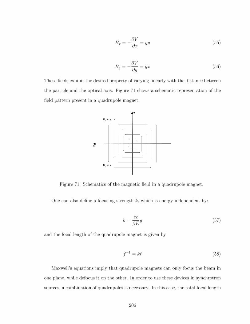
Bx = −∂V∂x
= gy (55)
By = −∂V∂y
= gx (56)
These fields exhibit the desired property of varying linearly with the distance between
the particle and the optical axis. Figure 71 shows a schematic representation of the
field pattern present in a quadrupole magnet.
Figure 71: Schematics of the magnetic field in a quadrupole magnet.
One can also define a focusing strength k, which is energy independent by:
k =ec
βEg (57)
and the focal length of the quadrupole magnet is given by
f−1 = k` (58)
Maxwell’s equations imply that quadrupole magnets can only focus the beam in
one plane, while defocus it on the other. In order to use these devices in synchrotron
sources, a combination of quadrupoles is necessary. In this case, the total focal length
206

f resulting from the combination of two lenses with two different focal lengths f1 and
f2 is
1
f=
1
f1
+1
f2
+d
f1f2
(59)
where d is the distance between the two lenses.
207
B Devices used to generate synchrotron light
B.1 Bending Magnets
The known circular trajectory electrons describe in synchrotron accelerators is
achieved with the use of magnets. If not for their action, the electrons would,
according to inertia laws, move in a straight line. The Lorentz force resulting of the
interaction between magnets and charged particles in the accelerator acts as a
centripetal force causing a circular trajectory (which connects stretches of straight
trajectories to generate the trajectory observed in accelerators) according to the
equation
mγv2κ+ e [v ×B] = 0 (60)
where κ = (κx, κy, 0) is the local curvature vector in the trajectory:
κx,y =1
ρx,y(61)
with ρx,y is the local radius of the trajectory [119].
In order to simplify the calculations for the particle beam dynamics, it is
considered that only the transverse component of the magnetic field (the component
normal to the velocity of the particles) acts on the particles. Considering that the
velocity components normal to the trajectory of the beam are negligible compared
to the total particle velocity, using equation 60, the bending radius for the electron
trajectory is given by
1
ρ=
∣∣∣∣epB∣∣∣∣ =
∣∣∣∣ ecβEB∣∣∣∣ (62)
where p = γmv and the so-called cyclotron or Larmor frequency, which represents
the frequency of revolution of a particle in its orbit, is [119]
208

ωL =
∣∣∣∣ec2
EB
∣∣∣∣ . (63)
When going through the bending magnets the two effects discussed previously
happen: the electron beam is bent into a curved trajectory and radiation is emitted
as the charged particles travel in a curved path [116].
Since radiation is emitted during the whole curved trajectory the beam goes
through, the collimation around narrow angle is lost in the horizontal direction, but
maintained in the direction perpendicular to the particle beam plane. A slit is used
in experiments to select the size of the horizontal radiation beam desired. The
radiation is, then, collected and summed incoherently in the collection angle given
by
4θ =w
D ψ (64)
where w is the width of the slit used, D is the distance from the electron orbit and
the slit and ψ is the vertical angle in which the radiation is distributed [116].
The power radiated in the synchrotron when relativistic electrons travel at a
circular orbit is given by the Schwinger’s formula:
Pe =
¨P (λ, ψ)dλdψ =
2
3
e2c
R2
[E
mc2
]4
(65)
where λ is the wavelength of the radiation emitted and R is the curvature radius in
the particles’ trajectory. This equation shows that Pe ∝ E4/R2, which means that, if
one wants to increase the energy in the storage rings, while maintaining the necessary
radiated power, one must also increase the radius of the ring. This equation also
shows that Pe ∝ m−4 and, therefore, electrons, due to their lower mass, will produce
more power radiated than more massive particles, such as protons, and that is the
reason most synchrotron facilities choose electrons to compose their particle beams
209
[116].
The radiation emitted by using a bending magnet has a broad spectrum, going
from x-rays to infrared, for which the describing function is called universal
synchrotron radiation function (G1). The synchrotron radiation spectral
distribution can be characterized by the critical wavelength λc, which is given by
λc =4
3πRγ−3 (66)
where γ = ψ−1. The critical wavelength determines the point in the radiation
spectrum that divides the radiation power emitted in half, i.e. 50% of the power is
emitted in wavelengths below the critical value, while the other 50% is emitted in
wavelengths above it [116].
This wide and continuous distribution spectrum can be explained by statistical
fluctuations on the energy of the electrons in the beam and around their orbit. They
are also influenced by the statistical nature of the light emission itself [116].
The number of photons with wavelength band of width ∆λ/λ, centered at λ, and
emitted by each electron moving in an arc with length R∆θ is given by
N(λ) =31/2
2π
e2
hRγG1
∆λ
λ∆θ (67)
where h is Planck’s constant and G1 is the universal synchrotron radiation function.
Thus, the total number of photons emitted by a storage ring is given by equation 67
multiplied by the number of electrons traveling in the ring, which is:
Ne =I (2πR)
ec(68)
where I is the beam current. Then,
Ntotal(λ) =31/2
hceγIG1
∆λ
λ∆θ (69)
210

This equation describes the spectral distribution of the universal synchrotron
radiation function, where it is noticeable that the distribution falls exponentially
when λ λc and falls slowly for λ λc, being, in this last case, mostly determined
by the electron beam current [116].
Another important parameter used to characterize a synchrotron source is the
critical energy, which is given by
εc =3hcγ3
4πR(70)
The radiation energy achievable by a synchrotron source is typically a few times the
critical energy [116].
The radiation emitted using bending magnets is mostly linearly polarized. The
polarization direction varies with respect to the angle in relation to the beam plane.
On the horizontal plane, the radiation emitted is completely polarized on the
horizontal direction (parallel to the beam plane). As one moves above or below such
plane, a perpendicular component appears [116].
B.2 Wigglers
Bending magnets must always be present in synchrotron rings, since they are
responsible for generating its circular trajectory. However, after the first generation
sources, insertion devices started being used to generate radiation. These devices do
not interfere with the overall circular trajectory of the beam and, therefore, can be
inserted in the ring along its straight pieces. They generate radiation by creating
small oscillations in the electron beam, using alternating magnets, maintaining,
however, the beam’s direction of movement along the ring. These devices not only
increase the amount of beamlines allowed in the facility, since they can be inserted
anywhere along the trajectory, but also allow for higher radiation energies (due to
211

the possibility of smaller angles of curvature); for higher radiation intensities, by
increasing the amount of oscillations (and, thus, magnetic poles present in the
device) the beam goes through; and for the increase in spectral brightness [116].
Wigglers were the first insertion devices developed to be used in synchrotron
sources, since their second generation. K. W. Robinson was the first to theorize the
use of such a device to generate radiation in synchrotron facilities in an unpublished
report in 1956 [130]. The first wiggler was built a decade later, in 1966, at the
Cambridge Electron Accelerator (CEA-14) [131] as a damping system for their beam
storage system. In 1979, the first wiggler was used in a synchrotron source at the
Stanford Synchrotron Radiation Lightsource (SSRL) and its success prompted other
synchrotron across the world to develop similar devices [130].
Wigglers are built as a set of magnets with alternating poles, which cause the
electrons to wiggle around a straight line. The magnetic field applied is usually
perpendicular to the beam plane, which results in the horizontal oscillation of the
electrons. Since these magnets are not being used to maintain the electron beam in
their orbit, they can be tuned to obtain a smaller radius of curvature when compared
to bending magnets, which results in the emission of radiation with higher energy
[116].
In commonly used units, the instantaneous radius of curvature of a charged
particle under the effect of magnetic field is
R(m) =3.34E[GeV ]
B[T ](71)
where E is the electron energy given in GeV and B is the intensity of the magnetic
field given in teslas. Using equation 70, also substituting the constants by their values,
and the previous result, the critical energy for a wiggler is given by
εc(keV ) = 0.665E2[GeV ]B[T ]. (72)
212
This result shows that the critical energy, and therefore the maximum photon energy
that can be reached at the storage ring, can be tuned according to the intensity of
the magnetic field chosen, independently of the energy of the electrons in the beam
[116].
The amount of magnetic poles, and, consequently, electron oscillations, present
in the wiggler will determine the gain in intensity compared to a bending magnet.
However, the construction of a wiggler must be such that the beam trajectory is not
changed once it goes through the device. For this to be possible, the first and last
magnets must have their effects mirrored and the magnetic field of each must be half
of that present in the intermediary magnets so the electrons will only complete half
of an oscillation [130].
One can see a wiggler device as a series of bending magnets, and, therefore, they
both produce radiation with the same spectral characteristics of a broad wavelength
bandwidth. However, since the radiation in the wiggler is produced by multiple beam
oscillations, it appears as a series of short pulses, instead of the single pulse produced
by a bending magnet. That is the cause for the device’s increase in radiation intensity
when compared to bending magnets [116]
In order to mathematically differentiate wigglers and undulators, one can use the
dimensionless parameter K, which is defined as “the ratio between the wiggling angle
of the trajectory, α and the natural aperture of synchrotron radiation 1/γ” [116]. Both
variables are defined in figure 72, which shows the electron oscillations in a wiggler
as well as the path described by the emitted radiation. The parameter K is, then,
written as
K = αγ (73)
which means that an electron moving in a sinusoidal trajectory will have K given by
213

K =e
2πmcλuB = 0.934λu[cm]B[T ] (74)
where λu is the period of the device.
Figure 72: Simplified representation of the electron oscillations within a wiggler, aswell as the radiation produced by their acceleration. (Original in colour)
In wigglers, the angle of trajectory is much larger than the opening angle ψ = 1/γ,
which means that K 1. In this case, the effects caused by interference between
radiation emitted in different poles can be neglected and the intensity of the radiation
produced can be obtained by integrating over the contributions of each oscillation
[116].
B.3 Undulators
The theoretical idea of undulators was first proposed by V. L. Ginzburg, in 1947 [133]
and they were first built by Hans Motz and coworkers in 1953 [134]. Soviet scientists
installed undulators in two synchrotrons in the 1970s for tests and gathered most
of the initial information on the properties of synchrotron light produced by these
devices [130].
Undulators have similar technology to that of wigglers, with the difference that the
magnetic field generated by each pole is designed such that the angle of the trajectory
α is smaller than, or close to, the opening angle ψ, in a way that the emission cone
remains within the device. In consequence, instead of the series of short pulses of
214
radiation seen with the use of wigglers, undulators produce a single long pulse. Also,
for undulators, K < 1 [116].
Since the emission angle is small in undulators, the interference between radiation
produced in different oscillations must be taken into account and the wavelength for
which the interference is constructive is given by the following equation when the
radiation is observed at an angle θ in relation to the undulator axis:
λ =λu2γ2
(1 +
K2
2+ γ2θ2
). (75)
As consequence of the interference, the spectrum of the radiation produced has a
very narrow wavelength bandwidth, centered on the peak photon energy hvc, which
is given by (derivation can be found on [116]):
hvc ≈2γ2hnc
Lu(76)
where Lu is the period of the undulator, γ is obtained with the use of Lorentz
contraction and Doppler effect arguments and can be written as
(c+ v
c− v
)1/2
=
[(c+ v)2
(c2 − v2)
]1/2
=(
1 +v
c
)[ 1
1− v2
c2
]1/2
≈ 2γ (77)
and n is an integer that corresponds to the n-th harmonic of the wavelength that suffer
constructive interference λn = λ/n [116]. The amount and intensity of the harmonics
increase with K, while when θ = 0, i.e. on the undulator axis, only odd harmonics
can be produced [116].
Since K ∝ B (equation 74), the wavelength λ ∝ B2. Therefore, one can tune
undulators to produce the desired wavelength by changing their magnetic field. And
while in wigglers the radiation emitted in each period adds up, increasing with 2N ,
where N is the number of periods, in undulators the radiation adds coherently,
increasing with N2 [116].
215

The small emission angle together with the increase in intensity with N2 mean
that the brightness reached with undulators is much higher than what can be
achieved with any other devices [116]. The choice of the method to produce
radiation, however, depends on the experiment intended: if brightness is the most
important characteristic, undulators are the best choice, but if a broad spectrum is
necessary, wigglers should be used.
216
C X-ray interactions with matter and optics
Interactions between X-rays and matter are particularly interesting in the study of
materials due to the characteristics of this type of electromagnetic radiation, since it
has wavelengths in the same order of magnitude as the distance between atoms in
solids and liquids and it has a relatively large penetration depth in samples.
Different kinds of interactions include absorption, scattering or diffraction,
refraction and emission and they will be explained in more detail in the next
sections [123].
C.1 Scattering
Classically, the scattering of an X-ray by a single electron is described as the
interaction between the incident wave and the electron, which suffers the action of
electromagnetic force causing its acceleration and consequent emission of a scattered
wave with the same wavelength as the incident one. Therefore, classically, this
process is always elastic. Considering quantum aspects, the scattering may be
inelastic, since the photon can transfer energy to the electron, resulting on a
scattered photon with energy smaller than the incident one. This phenomenon is
known as Compton effect. Considering the elastic case and the fact that momentum
can be transferred to the electron, in this case, as well, one can define
~Q = ~k − ~k′ (78)
where ~k and ~k′represent the initial and final momenta for the photon, respectively,
and the vector Q is the wavevector transfer or scattering vector, which is commonly
used to describe scattering processes [135].
According to classical principles, in the simplest scattering case, the interaction
of an X-ray with a single electron would make it vibrate, making it act like a dipole
217

antenna, emitting radiation. The radiated field at a point X at a distance R from
the electron and at angle ψ with respect to the direction of the incident light can be
derived using Maxwell’s equation (see [135] for derivation):
Erad(R, t) = − −e4πε0c2R
aX(t′) (79)
where −e is the charge of an electron, c is the speed of light, ε0 is the vacuum
permittivity and aX(t′) is the acceleration seen by the observer at X, measured at a
time t′ before the observation time t, given by t′ = t− R/c [135].
The acceleration aX(t′) is measured from the observer, which means that if ψ = π/2,
aX(t′) = 0, while it reaches its maximum value when ψ = 0. This behaviour is explicit
in the equation for the acceleration:
aX(t′) =−emEx0e
−iωt′ cosψ =−emEine
iω(Rc ) cosψ (80)
where Ein = Ex0e−iωt′ is the electric field of the incident X-ray. Using this result,
equation 79 can be rewritten as
Erad(R, t) = − −e4πε0c2R
−emEine
iω(Rc ) cosψ (81)
and the ratio between radiation emitted and incident is given by:
Erad(R, t)
Ein= −
(e2
4πε0mc2
)eikR
Rcosψ (82)
where k = ω/c, eikR/R represents a spherical wave and the term in brackets that precedes
it is called Thomson scattering length (or classical electron radius):s
r0 =
(e2
4πε0mc2
)= 2.82× 10⁻⁴nm (83)
This scattering length determines the ability an electron has to scatter an incident
218

wave [135].
An important result of equation 82 is related to the negative symbol, which means
that the two waves, incident and radiated, have a phase difference of 180 or, in radians,
π [135].
This classical description of the interaction between the X-ray and the electrons
is called Rayleigh-scattering. For incident radiation with electric field randomly
distributed in direction:
Iscat = I01
r2
(e2
m0c2
)2 (1 + cos2 θ
)(84)
where Iscat is the intensity of the scattered radiation, I0 is the intensity of the incident
light, r is the distance to the observation position, e is the charge of the electron, m0
is the mass of the electron and θ is the scatter angle. According to this equation,
then, the energy of the scattered light is not different from the energy of the incident
light, however its intensity depends on the scatter angle [123].
If the X-ray is interacting with an atom instead, the binding energy between the
electron and the atom must be considered. If the incident energy is approximately the
same as the binding energy of the electron to the atom, then one would expect that the
scattering length to decrease considerably. The length increases as the incident beam
energy increases or as the binding energy decreases (i.e., if the electron is farther from
the nucleus). For beam energies much higher than the binding energy, the electrons
can be treated as free [135].
In the case of a single molecule, the scattering length is much smaller than for
an atom and measurements cannot be taken using any X-ray source available today.
In order to measure molecules, they must be organized into crystals to amplify the
signal. In this case, the scattering only happens in determined angles, according to
Bragg’s law:
219
mλ = 2d sin θ (85)
where m is an integer, d is the distance between planes in the crystal, and θ is the
incidence angle. When on the Bragg angle, the light interferes constructively and the
signal gets stronger than for a single molecule. For all other angles the interference
is destructive and a signal cannot be measured [135].
The previous discussion is based on elastic scattering of light by electrons,
which, as already mentioned, is the classical description of the interaction. However,
quantum mechanics allow for inelastic collisions. For these conditions one must
assume the incoming X-ray is composed of a beam of photons. In this case, energy
can be transferred from the incoming photon to the electron and, therefore, the
scattered photon will have an energy smaller than the initial one [135, 136]. This is
the Compton effect and it is mathematically described by the following equation
[136]:
λ2 − λ1 =h
mc(1− cos θ) . (86)
This equation shows that the change in the energy of the scattered radiation depends
on the scatter angle, such that it is minimum when θ = 0, i.e. there is no collision,
and maximum at θ = 180, i.e. when the collision is head-on [123].
While both types of interaction happen in a sample, the relative intensity
between inelastic and elastic scatterings depends on the composition of the sample.
While elastic scattering is mostly independent on the sample matrix, the inelastic
portion depends on the atomic number of the elements present in it. The intensity
of the inelastic scattering is large for low atomic numbers and decreases as the
atomic number increases. This relationship can also be used to estimate the average
atomic number in the sample matrix [123].
220

C.2 Absorption
When a photon interacts with an atom, it can also be absorbed. The photon’s energy
is, then, transferred to an electron, which will either move to a higher energy level
within the atom or, if the energy is enough, will leave the atom completely, becoming
a free electron and leaving the atom ionized. This mechanism is mathematically
described by the linear absorption coefficient µ. The intensity of radiation going
through a sample is given by
−dI = I(z)ρadzσa = I(z)µdz (87)
where µdz corresponds to the attenuation of the beam through a sample of thickness
dz and the intensity is measured at a distance z from the surface of the material [135].
The attenuation coefficient can be written as:
µ = ρaσa =
(ρmNA
A
)σa (88)
where NA is Avogadro’s number, ρm is the mass density and A is the atomic number
of the element in the sample [135].
The solution of this equation is
I(z) = I0e−µz (89)
where I0 is the intensity of the beam at z = 0. That means µcan be obtained
experimentally by measuring the intensity of the beam with and without going
through a sample [135].
The mass attenuation coefficient for a compound material is given by the average
µcompound =∑
wiµi (90)
221

where wi is the mass fraction of element i and µi is the mass attenuation coefficient
for element i [123].
Analyses using X-ray absorption were the first to be developed, virtually at the
same time that X-rays themselves were discovered by Roentgen. The most famous
X-ray image, of his hand with a ring, is an example of the use of X-ray absorption
to visualize internal structures in people, which is still, probably, the most common
application of X-rays. Since people’s bodies are made up of different tissues, with
different attenuation coefficients, the amount of radiation able to go through the
body depends on the kind of tissue it finds in its way, which generate patterns related
to the disposition of tissues in the body [123].
Using the same absorption principle, but taking images from different directions
of the sample, one can reconstruct the whole sample in three dimensions, including
internal structures. This technique is called X-ray tomography and it is another
application of X-ray absorption to characterize materials [123].
A common requirement for all absorption techniques, however, is the choice of
radiation energy. The energy should be such that X-rays can pass through the
sample chosen, while, at the same time, providing enough contrast between different
structures, i.e. it must provide attenuation coefficients different enough for each
studied structure [123].
C.3 Refraction
There are two ways that a scattered wave can interact with the incident wave,
depending on their phase difference: when there is no phase shift between them, the
refractive index n > 1; and when there is a phase shift of π between them, the
refractive index n < 1. In the case of incident x-rays, the phase difference is π [135],
as previously discussed.
Assuming there is no absorption by the material and the interface between a
222
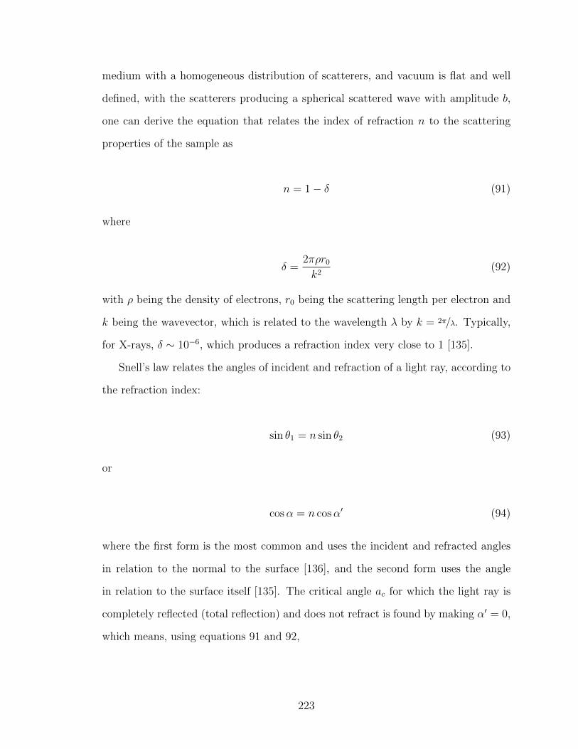
medium with a homogeneous distribution of scatterers, and vacuum is flat and well
defined, with the scatterers producing a spherical scattered wave with amplitude b,
one can derive the equation that relates the index of refraction n to the scattering
properties of the sample as
n = 1− δ (91)
where
δ =2πρr0
k2(92)
with ρ being the density of electrons, r0 being the scattering length per electron and
k being the wavevector, which is related to the wavelength λ by k = 2π/λ. Typically,
for X-rays, δ ∼ 10−6, which produces a refraction index very close to 1 [135].
Snell’s law relates the angles of incident and refraction of a light ray, according to
the refraction index:
sin θ1 = n sin θ2 (93)
or
cosα = n cosα′ (94)
where the first form is the most common and uses the incident and refracted angles
in relation to the normal to the surface [136], and the second form uses the angle
in relation to the surface itself [135]. The critical angle ac for which the light ray is
completely reflected (total reflection) and does not refract is found by making α′ = 0,
which means, using equations 91 and 92,
223
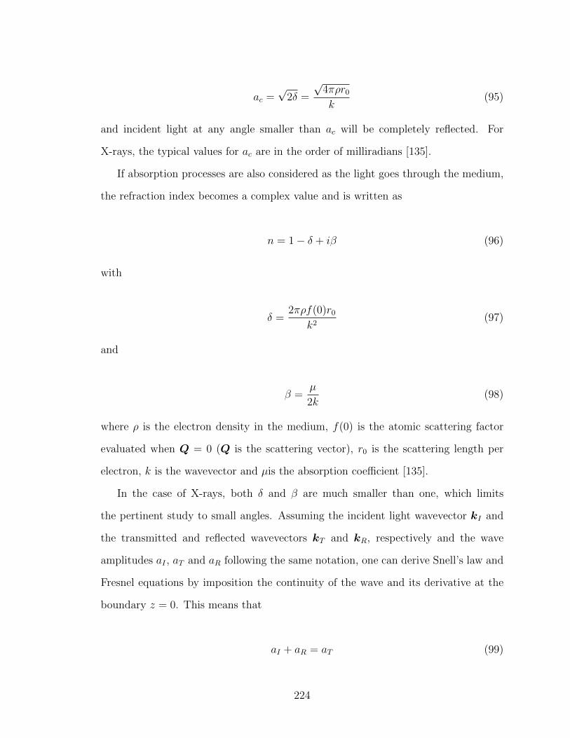
ac =√
2δ =
√4πρr0
k(95)
and incident light at any angle smaller than ac will be completely reflected. For
X-rays, the typical values for ac are in the order of milliradians [135].
If absorption processes are also considered as the light goes through the medium,
the refraction index becomes a complex value and is written as
n = 1− δ + iβ (96)
with
δ =2πρf(0)r0
k2(97)
and
β =µ
2k(98)
where ρ is the electron density in the medium, f(0) is the atomic scattering factor
evaluated when Q = 0 (Q is the scattering vector), r0 is the scattering length per
electron, k is the wavevector and µis the absorption coefficient [135].
In the case of X-rays, both δ and β are much smaller than one, which limits
the pertinent study to small angles. Assuming the incident light wavevector kI and
the transmitted and reflected wavevectors kT and kR, respectively and the wave
amplitudes aI , aT and aR following the same notation, one can derive Snell’s law and
Fresnel equations by imposition the continuity of the wave and its derivative at the
boundary z = 0. This means that
aI + aR = aT (99)
224

and
aIkI + aRkR = aTkT (100)
where in vacuum, |kI | = |kR| = k and in the material |kT | = nk [135]. Separating
the previous equation in components perpendicular and parallel to the surface of the
medium:
− (aI − aR) k sinα = −aT (nk) sinα′ (101)
aIk cosα + aRk cosα = aT (nk) cosα′. (102)
where α is the incident and reflected angle and α′ is the transmitted angle. Then,
combining the results from equations 99 and 102:
cosα = n cosα′ (103)
which is Snell’s law [135].
One can also combine the results of equations 99 and 101, resulting in
aI − aRaI + aR
= nsinα′
sinαuα′
α(104)
for small angles. From this relation, the Fresnel equations can be obtained:
r ≡ aRaI
=α− α′
α + α′(105)
t ≡ aTaI
=2α
α + α′(106)
where r and t are the amplitude reflectivity and transmittivity, respectively [135].
225

C.4 Reflection
The reflected amplitude discussed in the previous section using Fresnel equations is
valid when X-rays are shone onto an infinite slab of material, i.e., there is only one
interface to be crossed (usually, between vacuum and medium). This result changes
when the material is finite, since, in this case, multiple interfaces exist, resulting in
infinite possible reflections (figure 73) [135].
Figure 73: Schematic representation of incident light on a finite slab of material andsome of its possible reflections [113].
As can be seen in figure 73, a reflection can happen directly at the first interface
between vacuum and material, which is the same being considered on a infinite slab.
However, others are possible: the light can be transmitted through the material,
reflected on the interface between material and vacuum, transmitted again through
the material and pass through the vacuum-material interface again. In this case,
the final reflected amplitude must be made of a series of transmitted and reflected
amplitudes to describe the light’s path and interactions. It must also contain a phase
factor p2 = eiQ∆ [135]. Since infinite series of transmissions and reflections are allowed,
the total reflectivity amplitude must be given by
rslab = r01 + t01t10r12p2 + t01t10r10r
212p
4 + t01t10r210r
312p
6 . . . (107)
226

rslab = r01 + t01t10r12p2
∞∑m=0
(r10r12p
2)m
(108)
where the index 01 means interface 0 to 1 and so on [135].
Equation 108 is a geometric series, which can be summed to result on
rslab = r01 + t01t10r12p2 1
1− r10r12p2(109)
which can be simplified using equations 105 and 106 resulting on
rslab =r01 + r12p
2
1 + r01r12p2(110)
where p2 = eiQ1∆ and Q1 = 2k1 sinα1.
C.5 Emission
The absorption phenomenon discussed in the previous section can also generate the
emission of photons. When the photon is absorbed by an electron (considering the
energy of X-rays, this electron can even belong to the atom inner shells), this electron
will move to a higher energy level or leave the atom. This will leave a hole that must
be filled by an electron in a higher energy level, which will emit a photon with the
corresponding energy difference. The emitted photon is also, typically, in the X-ray
energy range. This process is called X-ray fluorescence and the energy of the emitted
photon E is related to the atomic number N of the atom according to Moseley’s law
E = C1 (Z − C2)2 (111)
where C1 and C2 are constants, which depend on the energy shells involved in the
process [123].
The intensity of the radiation emitted depends on the intensity of the incident
227

radiation, on the mass attenuation coefficient for the material and on the probability
of the specific transition of the electron in a higher energy level to the lower level.
Also, it depends on the probability that an Auger electron is emitted. That happens
when instead of the excess energy being released as a photon, it is transferred to
another electron of the atom, giving it energy to leave [123]. Fluorescence yield ω is
what the probability of the X-ray emission is also called, and it depends on the atomic
number of the atom and on the electron transition involved, and it is mathematically
given by
ω =Xs
Xs + As(112)
where Xs i s the emission probability of a fluorescence photon and As is the emission
probability of a Auger electron [116].
The total de-exitation probability (i.e., emission of a fluorescence photon or Auger
electron added) is inversely proportional to the core-hole lifetime τh, which is smaller
for atoms with higher atomic number and, consequently, larger number of upper
energy levels and options of electrons, which can occupy the hole. This value is
related to the energy width of the excited state Γh due to the uncertainty principle
by Γhτh ' h, which is related to the resolution of absorption peaks. For a fixed edge,
the larger the atomic number, the smaller the core-hole lifetime and the larger the
energy width [116].
X-ray fluorescence can be used in materials characterization, as will be discussed
in the next sections of this paper (see section 2.6), to determine the composition of
samples. It can be used in qualitative way, in order to determine which elements are
present, and also in a quantitative way, since the number of photons detected for a
certain energy depends on the concentration of the element in sample [123].
228
C.6 Diffraction
When the X-ray scattering happens in a periodic crystal, the scattered light from
different planes in the crystal interfere such that the resulting light can only be
measured in some angles, where the interference is constructive. This angle depends
on the energy of the radiation and it is given by Bragg’s law:
nλ = 2d sin θ (113)
where n is an integer, λ is the wavelength of the scattered light, d is the interplanar
distance for the crystal and θ is the scatter angle [123].
Bragg’s law for X-ray diffraction offers the possibility of using different techniques
for materials characterization. The law presents only three parameters, making it
possible to design experiments such that one parameter is fixed, one is measured and,
then, the other can be calculated. One of these techniques is X-ray diffraction (XRD),
where, typically, the wavelength is fixed, the angle is measured and the interplanar
distance is calculated providing information on the lattice structure of the material
being measured [123].
229
D Detectors and detector artifacts
Energy dispersive detectors (i.e., detectors capable of obtaining information on a
photon’s energy) are necessary for X-ray fluorescence measurements. The different
types of these detectors can be classified into gas filled detectors and semiconductor
detectors.
Gas filled detectors use the ionization of the gas resulting of the interaction with
the incident X-rays to detect the photons. They are filled with an inert gas, which will
not react with the radiation, such as argon, kryptonium or xenon and a quench gas,
responsible for avoiding avalanche processes in the gas. Since quench gases can change
chemically during the detection, they are consumed with the use of the detector and,
therefore, in a sealed detector, they determine the detector’s lifetime. A way to
prevent that is to use a flow counter, which introduces gas in the detector as necessary
to maintain a constant level. This last kind of detector is specially used when detecting
elements with low atomic number, since the detector in this case must have a very
thin entrance window, which does not avoid completely atmospheric contamination
and, therefore, the continuous flow of quench gas is necessary for maintaining the
detecting properties of the detector [123].
The proportional scintillation counter is a combination of gas and scintillation
detectors. In this case, the detector uses the recombination energy (i.e., when the free
electrons recombine with the ions from the gas after being ionized by the radiation),
typically in the order of 20 to 40 eV. These photons are captured and amplified by the
scintillator, which improves the energy resolution of the detector. However, due to
the difficulty in producing these detectors, they are not available commercially [123].
The most common detectors for X-ray fluorescence measurements, however, are
semiconductor detectors. These detectors can be built using a series of materials,
but the most common choice is silicon, because it provides a good combination of
parameters important for an efficient detection, such as a small amount of energy
230

necessary for the creation of a charge carrier pair, which has a relatively long lifetime,
resistance against radiation damage and facility in production [123].
Silicon-based detectors have a better energy resolution than gas filled detectors,
typically in the range of 120 to 200 eV, but they lose in terms of count rate capabilities
and detection areas, which are usually in the order of a few 10 mm2 [123].
In energy dispersive detectors, the number of charge carriers produced is
proportional to the energy of the photon detected:
N =E
ε(114)
where N is the number of charges, E is the energy of the absorbed radiation and ε is
the amount of energy necessary to produce each charge. Therefore, for each detection,
the charge carrier pulse heights are measured and assigned to an energy channel. Since
photons with the exact same energy can be affected by different noises, the height
of peaks from photons with the same energy will differ slightly and, as result, the
heights corresponding to each energy are given by a Gaussian distribution [123].
The detected energy spectrum from a sample can show structures, which are not
the result of fluorescence emissions, but are caused by other factors [123]. They
will be discussed in the following sections, which are based on reference [123], unless
otherwise marked.
D.1 Detector response function
The detector response function influences the spectrum intensity distribution,
according to various factors, such as the broadening of the measured peaks
discussed above, due to the statistical fluctuations in the energy detected caused by
noise in the detector.
Another factor that may contribute to the response function is incomplete charge
231

collection, which can be caused by the recombination of charges along the path from
where they are generated until they reach the cathodes/. This effect would decrease
the amount of measured charges, causing a continuous contribution to the lower
energies of a peak called shelf; and by the impossibility of measuring all the charges
created by a photon when its absorption happens very close to the detector entrance
window (some of the charges end up in the window), which causes a tail also on the
low energy side of the peak that depends on the energy of the incident photon due
to the fact that lower energy photons have an increased probability to be absorbed
close to the entrance window when compared to higher energy ones. The first effect
can be reduced by using a detector material with better quality and the second can
be reduced by using special window materials.
D.2 Escape peak
Escape peaks are peaks produced when the incident photon produces a fluorescence
photon in the detector material, which, then, leaves the detector. When this happens,
the peak measure by the detector appears to have an energy smaller than it should,
considering the energy of the absorbed photon:
Eesc = Einc − Efluor (115)
where Eesc is the energy where the escape peak appears, Einc is the energy of the
incident photon and Efluor is the energy of the fluorescence photon produced in the
detector.
The probability of an escape peak being formed depends on the energy of the
incident photon. If the photon has energy below the edge of the detector material,
the probability is zero, since this photon will not be able to cause the excitation of the
atom’s electrons. If the energy is above the edge energy for the material, then lower
232

energy photons will have a larger probability to generate escape peaks, since they
are usually absorbed closer to the surface of the detector when comparing to higher
energy photons. When the photon is absorbed farther from the detector surface, it
has to travel a larger distance to escape the detector, increasing the probability that
the produced fluorescence photon will still be absorbed by the detector and will not
escape.
D.3 Pile up peaks
When two photons are detected at the same time (i.e., when the time interval between
them is smaller than the time resolution of the detector) the signal from the two pulses
may be added. The result is a peak at the energy corresponding to the sum of the
energy of the two detected photons.
The probability of such an overlap increases for more intense energy peaks, since
they are result of more photons being detected at such energy. The pile up peak
intensity, therefore, is given by
ISum = IMother1IMother2P (116)
where IMother1 and IMother2 refer to the intensity of the mother peaks (i.e., peaks with
the same energy as the photon being overlapped) and P is the probability for sum
peak as a function of shaping time and energy.
The pile up peaks need to be identified as such so that they are not assigned to
an element in the spectrum analysis. One way of doing so is by changing the
excitation intensity and plotting the results normalized in relation to a peak, which
is surely identified as an element’s spectral line. In this case, as the excitation
intensity increases or decreases, the intensity of the elemental peaks will also
increase or decrease proportionally, maintaining a constant ratio. However, since
233

pile up peak intensities are the result of a multiplication of the intensities of two
other peaks, their change with excitation intensity will be squared. Thus, when
comparing the normalized spectra, all the peaks will look the same, except the pile
up peaks, which will have increased or decreased in intensity much more than the
elemental peaks.
Pile up peaks can also be handled mathematically, using equation 116 to calculate
their intensity and applying these values to the spectrum fitting. This approach is
necessary when a pile up peak coincides with the spectral line of an element measured
and it is a way to isolate their intensities.
D.4 Scattering peaks
Scattering peaks are usually a small effect, but can still cause misidentifications in
the spectrum analysis. They are the result of X-rays being scattered in the
spectrometer and are not a result of sample measurement. Some common effects
include the excitation of the argon in the atmosphere, resulting on a peak in its
corresponding energy in the final spectrum (this can happen when the measurement
is not taken under vacuum conditions); the scattering of fluorescence radiation at
the detector’s collimator or envelope, which usually generates small peaks for
uncommon elements, such as zirconium; and scattered radiation form the sample,
which excites parts of the spectrometer, resulting on small peaks, which can be
misconstrued as trace elements.
D.5 Diffraction peaks
If the sample is crystalline or has crystalline areas, the appearance of diffraction peaks
is possible. The energy of the radiation diffracted is given by
E = 1, 242n
2dsin θ (117)
234

where n is an integer, d is the interplanar distance in the crystal and θ is the angle
between beam and sample.
For polycrystalline samples (i.e., samples in which the crystals are oriented in
many different directions), a large energy range can be diffracted in small quantities.
These diffractions, however, involve a small portion of the beam and do not have
large intensity. In this case, the result is an overall increase of the background for the
energy range in question. In micro-XRF, however, since the beam shines in a very
small region, not all directions of crystals are present, resulting in higher intensity
peaks with very specific energies, which do not correspond to elemental spectral lines.
It is difficult to correct the measured spectra for diffraction peaks, so the best
procedure is to try to avoid them at the time of the measurement or to find
experimental ways to identify them. These techniques can include measuring the
same sample in different scatter angles, which would also change the energy of the
diffraction peaks, but not the energy of the fluorescence peaks; identifying the
peaks, using the fact that diffraction peaks may not correspond to any element or,
when it does, they will not present the other lines in the element series, or that
diffraction peaks are usually not Gaussian in shape; and using filters to reduce the
radiation in the continuous part of the spectrum.
235

E Software used to reconstruct ant map
This is the code used to reconstruct the map for the North Carolina amber inclusion
(NC 272-276) from chapter 5. The software was written in C++ using the Cern
ROOT framework.
/***** Program deve loped to f i t s p e c t ra from SXRMB beamline from CLS −
map recons t ruc t i on , g l u i n g two maps . Using f i t t i n g background
methods from TSpectrum and f i t t i n g peaks wi th Gausians .
******/
#include<s t d i o . h>
#include<fstream>
#include<iostream>
#include<s t r i n g . h>
#include<TApplicat ion . h>
#include<TCanvas . h>
#include<TSpectrum . h>
#include<TMath . h>
#include<TH1. h>
#include<TLegend . h>
#include<TF1 . h>
#include<TH2. h>
#include<TH2F. h>
#include<TFile . h>
#include<TPolyMarker . h>
TApplicat ion myapp( ”myapp” , 0 , 0 , 0 , 0 ) ;
using namespace std ;
int s i z e =2048;
int nElement ;
int po intsx1 ;
236

int po intsy1 ;
f loat lowx1 ;
f loat highx1 ;
f loat lowy1 ;
f loat highy1 ;
int add1 ;
int po intsx2 ;
int po intsy2 ;
f loat lowx2 ;
f loat highx2 ;
f loat lowy2 ;
f loat highy2 ;
int add2 ;
char kind [ 4 ] ;
f loat cur rent ;
char nameElement [ 2 0 ] ;
f loat posElement ;
f loat areaError ;
f loat area ;
F l o a t t *pSpec=new float [ s i z e ] ;
TH1 * rawSpec ; //raw spectrum
TH1 *backSpec ; // spectrum wi thout the background
TH1 *background ; // background
TH1 * concent ra t i on=new TH1F( ” Concentrat ion ” , ” Concentrat ion ” , 1000 , 0 ,
2) ;
TH2 *map ;
TCanvas *c=new TCanvas ( ) ;
TCanvas *cBack=new TCanvas ( ) ;
TCanvas *cMap=new TCanvas ( ) ;
TCanvas *cConc=new TCanvas ( ) ;
237

TF1 *gaus1 ;
TList * f u n c t i o n s ;
TPolyMarker *tpm ;
TSpectrum * sp ;
i f s t r e a m input1 ;
i f s t r e a m input2 ;
i f s t r e a m elementData ;
i f s t r e a m c o r r F i l e 1 ;
i f s t r e a m c o r r F i l e 2 ;
TFile * f i l e ;
// openFi le opens the input F i l e
bool openFi l e (char inDir [ ] , char inName1 [ ] , char inName2 [ ] , char outDir
[ ] , char name [ ] )
input1 . open (Form( ”%s%s Bruker 1 . mca” , inDir , inName1 ) ) ;
i f ( ! input1 )
std : : cout << ”ERROR − Input 1 f i l e does not e x i s t ” << std : : endl ;
return fa l se ;
input1 . c l e a r ( ) ;
input1 . seekg (0 , i o s : : beg ) ;
input2 . open (Form( ”%s%s Bruker 1 . mca” , inDir , inName2 ) ) ;
i f ( ! input2 )
std : : cout << ”ERROR − Input 2 f i l e does not e x i s t ” << std : : endl ;
return fa l se ;
input2 . c l e a r ( ) ;
input2 . seekg (0 , i o s : : beg ) ;
f i l e=new TFile (Form( ”%s%s %s . root ” , outDir , inName1 , name) , ”RECREATE”
) ;
i f ( ! f i l e )
std : : cout << ”ERROR − Could not c r e a t e output f i l e ” << std : : endl ;
238
return fa l se ;
elementData . open ( ” ListElements . dat ” ) ;
i f ( ! elementData )
std : : cout << ”ERROR − Element data f i l e does not e x i s t ” << std : : endl ;
return fa l se ;
elementData . c l e a r ( ) ;
elementData . seekg (0 , i o s : : beg ) ;
c o r r F i l e 1 . open (Form( ”%s%s 1 . dat ” , inDir , inName1 ) ) ;
i f ( ! c o r r F i l e 1 )
std : : cout << ”ERROR − Correc t ion f i l e ” << inDir << inName1 << ” does
not e x i s t ” << std : : endl ;
return fa l se ;
c o r r F i l e 1 . c l e a r ( ) ;
c o r r F i l e 1 . seekg (0 , i o s : : beg ) ;
c o r r F i l e 2 . open (Form( ”%s%s 1 . dat ” , inDir , inName2 ) ) ;
i f ( ! c o r r F i l e 2 )
std : : cout << ”ERROR − Correc t ion f i l e ” << inDir << inName2 << ” does
not e x i s t ” << std : : endl ;
return fa l se ;
c o r r F i l e 2 . c l e a r ( ) ;
c o r r F i l e 2 . seekg (0 , i o s : : beg ) ;
return true ;
bool i n i t i a t e V a r ( int nx1 , f loat lx1 , f loat hx1 , int ny1 , f loat ly1 , f loat
hy1 , int ad1 , int nx2 , f loat lx2 , f loat hx2 , int ny2 , f loat ly2 ,
f loat hy2 , int ad2 , char name [ ] , char type [ ] )
po intsx1=nx1 ;
po intsy1=ny1 ;
239

lowx1=lx1 ;
highx1=hx1 ;
lowy1=ly1 ;
highy1=hy1 ;
add1=ad1 ;
po intsx2=nx2 ;
po intsy2=ny2 ;
lowx2=lx2 ;
highx2=hx2 ;
lowy2=ly2 ;
highy2=hy2 ;
add2=ad2 ;
s t r cpy ( nameElement , name) ;
s t r cpy ( kind , type ) ;
i f ( ( strcmp ( kind , ” l i n ” ) !=0)&&(strcmp ( kind , ” l og ” ) !=0) )
std : : cout << ”Parameter f o r kind o f map i n v a l i d . Options : l og and l i n ”
<< std : : endl ;
return fa l se ;
for ( int i =0; i <36 ; i++)
s t r i n g l i n e ;
g e t l i n e ( co r rF i l e 1 , l i n e ) ;
for ( int i =0; i <36 ; i++)
s t r i n g l i n e ;
g e t l i n e ( co r rF i l e 2 , l i n e ) ;
std : : cout << ” I n i t i a t i n g v a r i a b l e s ” << std : : endl ;
s td : : cout << ”Map s i z e : ” << ( po intsx1+add1 ) << ” X ” << ( po intsy1+
pointsy2 −1) << std : : endl ;
map=new TH2F( ”Map” , Form( ”Map − %s ” , nameElement ) , ( po intsx1+add1 ) ,
lowx1 , highx2 , ( po intsy1+pointsy2 ) , lowy1 , highy2 ) ;
240

return true ;
bool r e a d F i l e ( int mapN)
char temp [ 2 0 ] ;
int vbin ;
int bin =0;
i f (mapN==1)
input1 >> temp ;
do
input1 >> temp ;
vbin=a t o i ( temp ) ;
rawSpec−>F i l l ( bin +1, vbin ) ;
pSpec [ bin ]= vbin ;
bin++;
while ( bin<s i z e ) ;
char pars [ 2 1 ] [ 2 1 ] ;
c o r r F i l e 1 >> pars [ 0 ] >> pars [ 1 ] >> cur rent >> pars [ 2 ] >> pars [ 3 ] >>
pars [ 4 ] >> pars [ 5 ] >> pars [ 6 ] >> pars [ 7 ] >> pars [ 8 ] >> pars [ 9 ]
>> pars [ 1 0 ] >> pars [ 1 1 ] >> pars [ 1 2 ] >> pars [ 1 3 ] >> pars [ 1 4 ] >>
pars [ 1 5 ] >> pars [ 1 6 ] >> pars [ 1 7 ] >> pars [ 1 8 ] >> pars [ 1 9 ] >> pars
[ 2 0 ] ;
else
input2 >> temp ;
do
input2 >> temp ;
vbin=a t o i ( temp ) ;
rawSpec−>F i l l ( bin +1, vbin ) ;
pSpec [ bin ]= vbin ;
bin++;
while ( bin<s i z e ) ;
241

char pars [ 2 1 ] [ 2 1 ] ;
c o r r F i l e 2 >> pars [ 0 ] >> pars [ 1 ] >> cur rent >> pars [ 2 ] >> pars [ 3 ] >>
pars [ 4 ] >> pars [ 5 ] >> pars [ 6 ] >> pars [ 7 ] >> pars [ 8 ] >> pars [ 9 ]
>> pars [ 1 0 ] >> pars [ 1 1 ] >> pars [ 1 2 ] >> pars [ 1 3 ] >> pars [ 1 4 ] >>
pars [ 1 5 ] >> pars [ 1 6 ] >> pars [ 1 7 ] >> pars [ 1 8 ] >> pars [ 1 9 ] >> pars
[ 2 0 ] ;
char pars [ 2 1 ] [ 2 1 ] ;
s td : : cout << ”Beam current ( c o r r e c t i o n ) : ” << cur rent << std : : endl ;
s td : : cout << ”************************** F i l e
******************************” << std : : endl ;
return true ;
bool c l o s e F i l e ( )
elementData . c l o s e ( ) ;
input1 . c l o s e ( ) ;
input2 . c l o s e ( ) ;
c o r r F i l e 1 . c l o s e ( ) ;
c o r r F i l e 2 . c l o s e ( ) ;
return true ;
// fitRawData draws and f i t s the h is tograms and save f i t t i n g parameters .
I t a l s o c a l c u l a t e s the area under the f i t t e d peaks boo l dra=f a l s e ;
bool fitRawData ( ) // draw histogram
elementData . c l e a r ( ) ;
elementData . seekg (0 , i o s : : beg ) ;
c−>cd ( ) ;
c−>SetLogy (1 ) ;
242

rawSpec−>Draw ( ) ;
sp−>Background ( pSpec , 2048 , 20 , TSpectrum : : kBackDecreasingWindow ,
TSpectrum : : kBackOrder2 , kFALSE, TSpectrum : : kBackSmoothing3 , kTRUE) ;
for ( int i =0; i<s i z e ; i++)
background−>F i l l ( i +1,pSpec [ i ] ) ;
background−>SetLineColor (2 ) ;
background−>Draw( ”SAME L” ) ;
cBack−>cd ( ) ;
for ( int i =0; i<s i z e ; i++)
backSpec−>F i l l ( i +1, rawSpec−>GetBinContent ( i +1)−background−>
GetBinContent ( i +1) ) ;
backSpec−>Draw ( ) ;
std : : cout << ”Background removal . . . DONE” << std : : endl ;
sp−>Search ( backSpec , 2 . 5 , ”nobackground” , 0 . 008 ) ;
f u n c t i o n s=backSpec−>GetListOfFunct ions ( ) ;
/******* I f automatic a l gor i thm cou ld f i nd peaks , i t w i l l i d e n t i f y
the de s i r ed peak by comparing i t to the expec ted energy and use
the energy from the peak f i n d e r to f i t and c a l c u l a t e the area .
In case the a l gor i thm cannot f i nd the de s i r e d peak , the
t h e o r e t i c a l va lue f o r the p o s i t i o n w i l l be used in s t ead *******/
i f ( funct i ons−>FindObject ( ”TPolyMarker” ) )
tpm=(TPolyMarker *) funct i ons−>FindObject ( ”TPolyMarker” ) ;
tpm−>SetMarkerSize ( 1 . 5 ) ;
tpm−>SetMarkerColor ( kGreen ) ;
Double t * posPeak=tpm−>GetX ( ) ;
int nPeaks=tpm−>GetN ( ) ;
std : : cout << nPeaks << ” peaks found” << std : : endl ;
nElement=nPeaks ;
char name [ 2 0 ] ;
char tEnergy [ 1 0 ] ;
f loat fEnergy ;
243

int foundPeaks [ 3 0 ] ;
int pCount=0;
do
elementData >> name >> tEnergy ;
fEnergy=a t o f ( tEnergy ) ;
i f ( strcmp ( nameElement , name)==0)
posElement=fEnergy /5+95;
i f ( strcmp (name , ”***” )==0)
continue ;
for ( int cnt =0; cnt<nPeaks ; cnt++)
i f ( ( ( posPeak [ cnt ]−95)*5 < fEnergy +50) && ( ( posPeak [ cnt ]−95)*5 >
fEnergy−50) )
std : : cout << ”Element : ” << name << ” − Energy : ” << ( posPeak [ cnt
]−95)*5 << ” eV” << std : : endl ; i f ( strcmp (
nameElement , name)==0)
posElement=posPeak [ cnt ] ;
foundPeaks [ pCount]= cnt ;
pCount++;
while ( strcmp (name , ”***” ) !=0) ;
for ( int i =0; i<nPeaks ; i++)
bool unk=true ;
for ( int t =0; t<pCount ; t++)
i f ( i==foundPeaks [ t ] )
unk=fa l se ;
i f ( unk )
std : : cout << ”Unknown peak − Energy : ” << posPeak [ i ]*10/2 << ” eV”
<< std : : endl ;
else
std : : cout << ”Peaks could not be found” << std : : endl ;
244

std : : cout << ”Using t h e o r e t i c a l va lue s f o r c a l c u l a t i n g area ” << std : :
endl ;
char name [ 2 0 ] ;
char tEnergy [ 1 0 ] ;
f loat fEnergy ;
do
elementData >> name >> tEnergy ;
fEnergy=a t o f ( tEnergy ) ;
i f ( strcmp ( nameElement , name)==0)
posElement=fEnergy /5+95;
std : : cout << ”Element : ” << name << ” − Energy : ” << fEnergy << ” eV
” << std : : endl ;
i f ( strcmp (name , ”***” )==0)
continue ;
while ( strcmp (name , ”***” ) !=0) ;
// f i t peaks
i f ( strcmp ( nameElement , ” Nikalpha ” )==0)
std : : cout << ” F i t t i n g . . . ” << nameElement << std : : endl ;
backSpec−>Fit ( gaus1 , ”Q” , ”” , posElement−20, posElement+30) ;
area=gaus1−>I n t e g r a l ( posElement−20, posElement+30) ;
areaError=gaus1−>I n t e g r a l E r r o r ( posElement−20, posElement+30) ;
else i f ( strcmp ( nameElement , ”Kkalpha” )==0)
std : : cout << ” F i t t i n g . . . ” << nameElement << std : : endl ;
backSpec−>Fit ( gaus1 , ”Q” , ”” , posElement−20, posElement+20) ;
area=gaus1−>I n t e g r a l ( posElement−20, posElement+20) ;
areaError=gaus1−>I n t e g r a l E r r o r ( posElement−20, posElement+20) ;
else i f ( strcmp ( nameElement , ”Cakalpha” )==0)
std : : cout << ” F i t t i n g . . . ” << nameElement << std : : endl ;
backSpec−>Fit ( gaus1 , ”Q” , ”” , posElement−40, posElement+20) ;
area=gaus1−>I n t e g r a l ( posElement−30, posElement+20) ;
245

areaError=gaus1−>I n t e g r a l E r r o r ( posElement−30, posElement+20) ;
else
std : : cout << ” F i t t i n g . . . ” << nameElement << std : : endl ;
backSpec−>Fit ( gaus1 , ”Q” , ”” , posElement−30, posElement+30) ;
area=gaus1−>I n t e g r a l ( posElement−30, posElement+30) ;
areaError=gaus1−>I n t e g r a l E r r o r ( posElement−30, posElement+30) ;
return true ;
bool plotMap ( int xpos , int ypos )
i f ( strcmp ( kind , ” l i n ” )==0)
i f ( area / cur rent *100<1)
map−>SetBinContent ( xpos , ypos , area / cur rent *100) ;
else
map−>SetBinContent ( xpos , ypos , 0) ;
i f ( strcmp ( kind , ” l og ” )==0)
map−>SetBinContent ( xpos , ypos , TMath : : Log10 ( area / cur rent ) ) ;
s td : : cout << ” Current : ” << cur rent << std : : endl ;
s td : : cout << nameElement << ” area : ” << xpos << ” , ” << ypos << ” = ”
<< area << std : : endl ;
s td : : cout << nameElement << ” normal ized area : ”<< map−>GetBinContent (
xpos , ypos ) << std : : endl ;
i f ( area !=0)
concentrat ion−>F i l l ( area / cur rent *100) ;
return true ;
bool MakeMap(char outDir [ ] , char inName1 [ ] , char opt [ ] )
for ( int j 1 =0; j1<po intsy1 ; j 1++)
for ( int i 1 =0; i1<po intsx1 ; i 1++)
rawSpec=new TH1F( ”Raw Spectrum” , ”Raw Spectrum” , 2048 , 0 , 2047) ; //
raw spectrum
246

backSpec=new TH1F( ”Spectrum ( no background ) ” , Form( ”Spectrum ( no
background ) − %i ,% i ” , i 1 +1, j 1 +1) , 2048 , 0 , 2047) ; // spectrum
wi thout the background
background =new TH1F( ”Background” , ”Background” , 2048 , 0 , 2047) ; //
background
gaus1=new TF1( ” gaus1 ” , ” gaus ” , 0 , 2048) ;
sp=new TSpectrum (100) ;
i f ( ! r e a d F i l e (1 ) )
std : : cout << ” Error read ing f i l e 1” << std : : endl ;
return fa l se ;
i f ( fitRawData ( ) )
std : : cout << ”Area c a l c u l a t e d s u c c e s s f u l l y ! ”<< std : : endl ;
else
std : : cout << ” F i t t i n g could not be performed ” << std : : endl ;
return fa l se ;
f i l e −>cd ( ) ;
rawSpec−>Write ( ) ;
backSpec−>Write ( ) ;
i f ( plotMap ( i 1 +1, j 1 +1) )
std : : cout << ”Map p lo t t ed ” << std : : endl ;
else
std : : cout << ” Error p l o t i n g map” << std : : endl ;
for ( int b=0; b<add1 ; b++)
area =0;
i f ( plotMap ( po intsx1+b+1, j 1 +1) )
std : : cout << ”Map p lo t t ed ” << std : : endl ;
else
std : : cout << ” Error p l o t i n g map” << std : : endl ;
247

rawSpec−>Delete ( ) ;
backSpec−>Delete ( ) ;
background−>Delete ( ) ;
gaus1−>Delete ( ) ;
sp−>Delete ( ) ;
for ( int j 2 =0; j2<po intsy2 ; j 2++)
for ( int b=0; b<add2 ; b++)
area =0;
i f ( plotMap (b+1, po intsy1+j2 +1) )
std : : cout << ”Map p lo t t ed ” << std : : endl ;
else
std : : cout << ” Error p l o t i n g map” << std : : endl ;
for ( int i 2 =0; i2<po intsx2 ; i 2++)
rawSpec=new TH1F( ”Raw Spectrum” , ”Raw Spectrum” , 2048 , 0 , 2047) ; //
raw spectrum
backSpec=new TH1F( ”Spectrum ( no background ) ” , Form( ”Spectrum ( no
background ) − %i ,% i ” , i 2 +1, j 2 +1) , 2048 , 0 , 2047) ; // spectrum
wi thout the background
background =new TH1F( ”Background” , ”Background” , 2048 , 0 , 2047) ; //
background
gaus1=new TF1( ” gaus1 ” , ” gaus ” , 0 , 2048) ;
sp=new TSpectrum (100) ;
i f ( ! r e a d F i l e (2 ) )
std : : cout << ” Error read ing f i l e 1” << std : : endl ;
return fa l se ;
i f ( fitRawData ( ) )
std : : cout << ”Area c a l c u l a t e d s u c c e s s f u l l y ! ”<< std : : endl ;
else
248
std : : cout << ” F i t t i n g could not be performed ” << std : : endl ;
return fa l se ;
f i l e −>cd ( ) ;
rawSpec−>Write ( ) ;
backSpec−>Write ( ) ;
i f ( plotMap ( add2+i 2 +1, po intsy1+j2 +1) )
std : : cout << ”Map p lo t t ed ” << std : : endl ;
else
std : : cout << ” Error p l o t i n g map” << std : : endl ;
rawSpec−>Delete ( ) ;
backSpec−>Delete ( ) ;
background−>Delete ( ) ;
gaus1−>Delete ( ) ;
sp−>Delete ( ) ;
f i l e −>cd ( ) ;
map−>Write ( ) ;
cMap−>cd ( ) ;
map−>SetSta t s (0 ) ;
map−>Draw( ”COLZ” ) ;
cConc−>cd ( ) ;
concentrat ion−>S e t T i t l e ( ” Concentrat ion ” ) ;
concentrat ion−>Draw ( ) ;
i f ( strcmp ( opt , ”no” )==0)
cMap−>SaveAs (Form( ”%s%s %s map−complete . png” , outDir , inName1 ,
nameElement ) ) ;
cConc−>SaveAs (Form( ”%s%s %s conc−complete . png” , outDir , inName1 ,
nameElement ) ) ;
else
249

cMap−>SaveAs (Form( ”%s%s %s %s map−complete . png” , outDir , inName1 ,
nameElement , opt ) ) ;
cConc−>SaveAs (Form( ”%s%s %s %s conc−complete . png” , outDir , inName1 ,
nameElement , opt ) ) ;
c l o s e F i l e ( ) ;
return true ;
// Main func t i on c a l l i n g a l l the ac t i on . Stops program i f anyth ing goes
wrong
int main ( int argc , char* argv [ ] )
std : : cout << ” Parameters : ” << argc << std : : endl ;
s td : : cout << ”Element : ” << argv [ 1 6 ] << std : : endl ;
i f ( argc !=22)
std : : cout << ” I n v a l i d number o f parameters \nProgram w i l l be c l o s e d ” <<
std : : endl ;
return 0 ;
i f ( openFi l e ( argv [ 1 ] , argv [ 2 ] , argv [ 9 ] , argv [ 1 8 ] , argv [ 1 6 ] ) )
std : : cout << ” F i l e s opened s u c c e s s f u l l y ” << std : : endl ;
else
std : : cout << ” I n v a l i d input f i l e ” << std : : endl ;
return 0 ;
i n i t i a t e V a r ( a t o i ( argv [ 3 ] ) , a t o f ( argv [ 4 ] ) , a t o f ( argv [ 5 ] ) , a t o i ( argv [ 6 ] ) ,
a t o f ( argv [ 7 ] ) , a t o f ( argv [ 8 ] ) , a t o i ( argv [ 2 0 ] ) , a t o i ( argv [ 1 0 ] ) , a t o f
( argv [ 1 1 ] ) , a t o f ( argv [ 1 2 ] ) , a t o i ( argv [ 1 3 ] ) , a t o f ( argv [ 1 4 ] ) , a t o f (
argv [ 1 5 ] ) , a t o i ( argv [ 2 1 ] ) , argv [ 1 6 ] , argv [ 1 7 ] ) ;
s td : : cout << ”Making map” << std : : endl ;
i f (MakeMap( argv [ 1 8 ] , argv [ 2 ] , argv [ 1 9 ] ) )
std : : cout << ”Map made s u c c e s s f u l l y ” << std : : endl ;
else
250

std : : cout << ” Error in map” << std : : endl ;
return 0 ;
std : : cout << ”**************END PROGRAM**************” << std : : endl ;
myapp . Run(1) ;
251
Related Documents
![METROLOGY WITH SYNCHROTRON RADIATION · 3 METROLOGY WITH SYNCHROTRON RADIATION When synchrotron radiation began to be utilized for spectroscopic investigations in the 1950s [1], the](https://static.cupdf.com/doc/110x72/5d4f2a0288c993720d8bc765/metrology-with-synchrotron-radiation-3-metrology-with-synchrotron-radiation.jpg)