Applications of permanent- magnet sources and arrays Francis F. Chen INER, February 24, 2009.

Applications of permanent-magnet sources and arrays

Francis F. Chen

INER, February 24, 2009

Helicon sources are ICPs with a DC B0

This is a commercial helicon source made by PMT, Inc. and successfully used to etch semiconductor wafers. It required two large and heavy electromagnets and their power supplies.

Computer chips are now etched with simpler sources without a DC B-field.

New applications require larger area coverage.

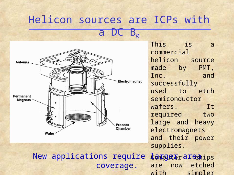
Possible uses of large-area plasma processing

Roll-to-roll plastic sheets

Smart windowsOLED displays

Solar cells, mass production Solar cells, advanced

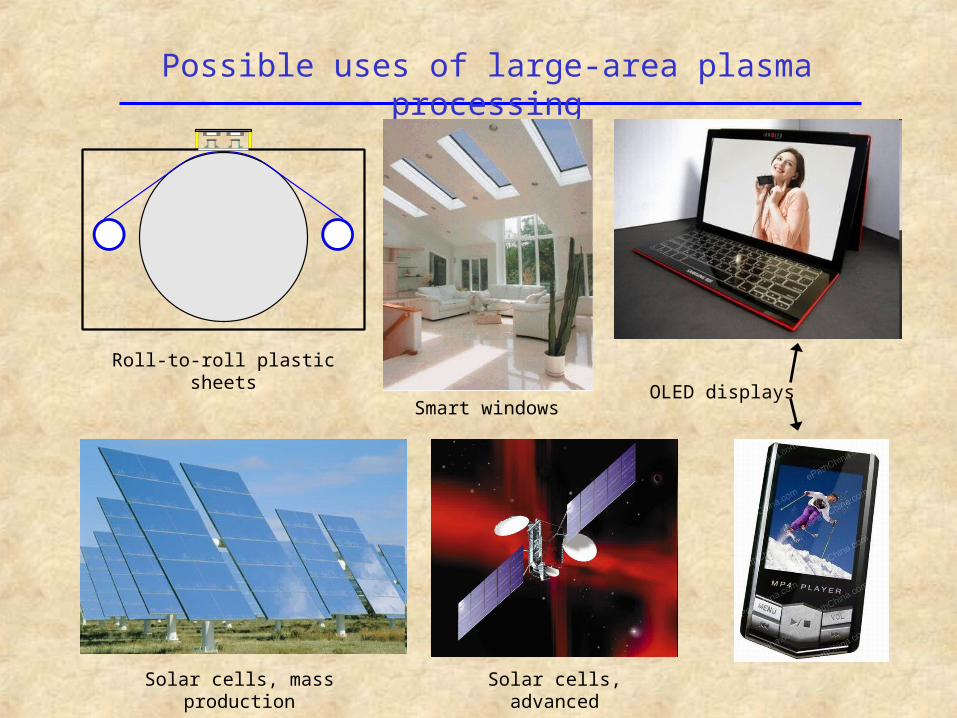
Distributed helicon source: proof of principle

ROTATING PROBE ARRAY

PERMANENT MAGNETS

3"

DC MAGNET COIL

18"

Power scan at z = 7 cm, 5 mT A, 20 G, 13.56 MHz,

0.0

0.5

1.0

1.5

2.0

0 5 10 15 20 25 30R (cm)

N (

101

2 cm

-3) 3.0

2.5

2.0

1.5

1.0

P(kW)

7-tube m=0 array

ARGON

PROBE

Achieved n > 1.7 x 1012 cm-3, uniform to 3%, but large magnet is required.F.F. Chen, J.D. Evans, and G.R. Tynan, Plasma Sources Sci. Technol. 10, 236 (2001)

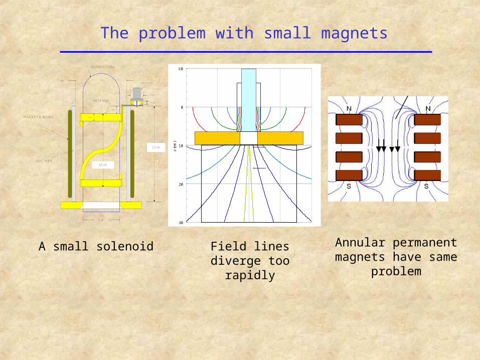
The problem with small magnets

-10

0

10

20

30

z (c

m)

QUARTZ TUBE

PVC PIPE

ANTENNA

MAGNET WINDING

7 cm

5 cm

13 cm

BNC connector

5 mm

17 mm

1 cm

1 cm

10 cm

Internal field

External field

Internal field

External fieldA small solenoid Field lines diverge

too rapidly

Annular permanent magnets have same

problem

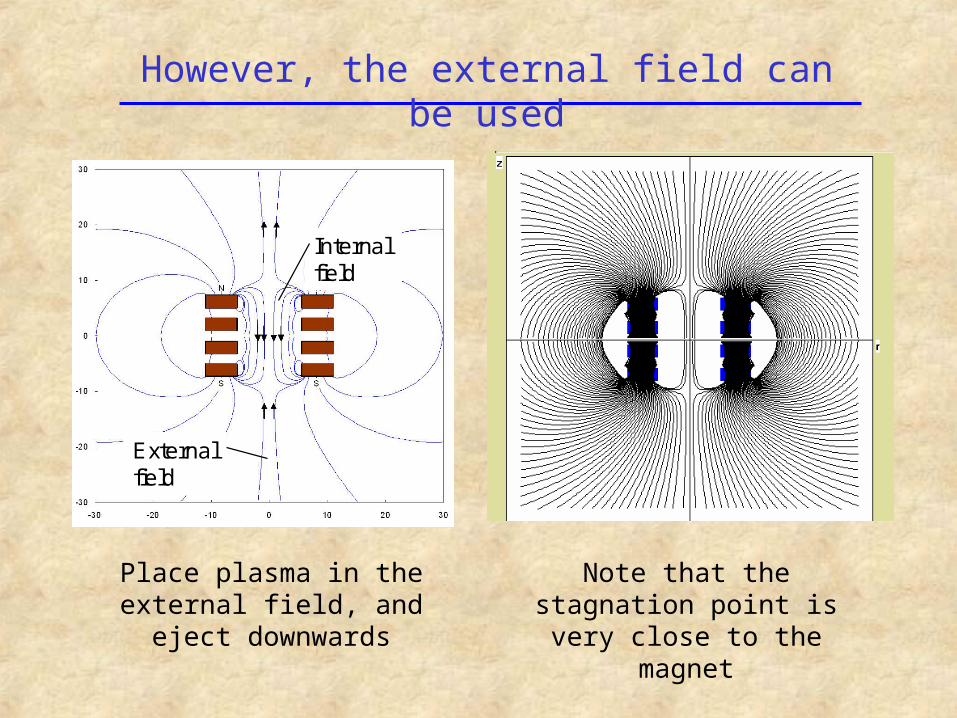
However, the external field can be used

Note that the stagnation point is very close to the magnet

Place plasma in the external field, and eject downwards

Internal field

External field

Internal field

External field

Gate Valve

To Turbo Pump

34 cm

36 cm

D

Z1

Z2

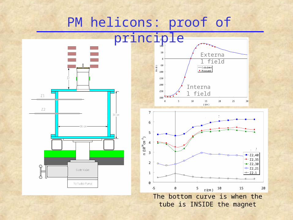
-300

-250

-200

-150

-100

-50

0

50

100

150

0 5 10 15 20 25 30

z (cm)

Bz

(G)

Calculated

Measured

External field

Internal field

0

1

2

3

4

5

6

7

-5 0 5 10 15 20r (cm)

n (

101

0cm

-3)

Z2, 40

Z2, 35

Z2, 30

Z2, 21

Z2, 1

D (cm)

500W, 1 mTorr

The bottom curve is when the tube is INSIDE the magnet

PM helicons: proof of principle

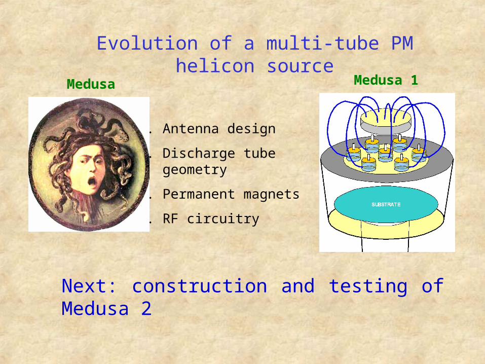
Evolution of a multi-tube PM helicon source

1. Antenna design

2. Discharge tube geometry

3. Permanent magnets

4. RF circuitry

Next: construction and testing of Medusa 2

Medusa Medusa 1

Helicon m = 1 antennas

--

+

E

B

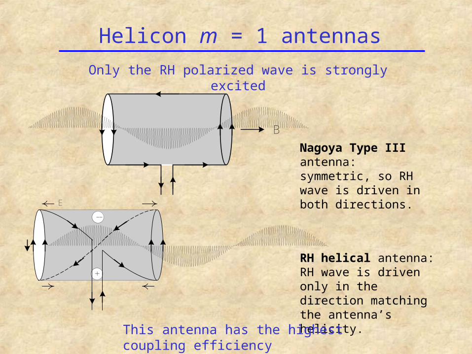
Only the RH polarized wave is strongly excited

Nagoya Type III antenna:symmetric, so RH wave is driven in both directions.

RH helical antenna:RH wave is driven only in the direction matching the antenna’s helicity.

This antenna has the highest coupling efficiency

Why we use an m = 0 antenna

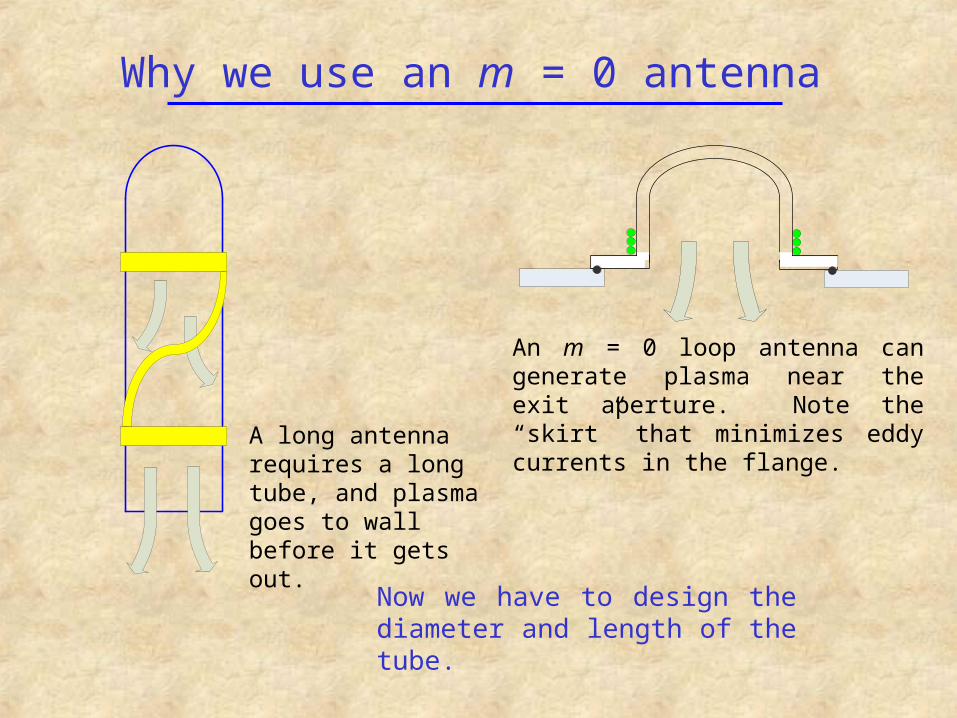
A long antenna requires a long tube, and plasma goes to wall before it gets out.

An m = 0 loop antenna can generate plasma near the exit aperture. Note the “skirt” that minimizes eddy currents in the flange.

Now we have to design the diameter and length of the tube.

The low-field peak: an essential feature

0.0

0.2

0.4

0.6

0.8

1.0

1.2

1.4

1E+11 1E+12 1E+13n (cm-3)

R (

oh

ms)

100.0

63.1

39.8

25.1

15.8

10.0

B(G) L=2", 1mTorr, conducting

Low-field peak

0.0

0.2

0.4

0.6

0.8

1.0

1.2

1.4

1E+11 1E+12 1E+13n (cm-3)

R (

oh

ms)

100.0

63.1

39.8

25.1

15.8

10.0

B(G) L=2", 1mTorr, conducting

Low-field peak

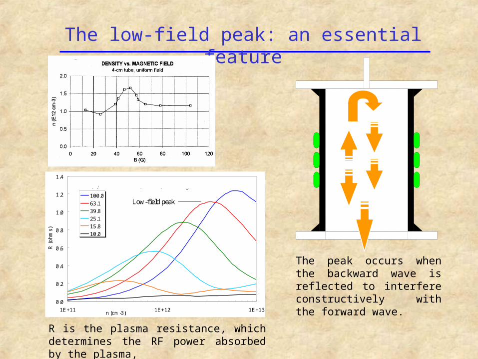
The peak occurs when the backward wave is reflected to interfere constructively with the forward wave.

R is the plasma resistance, which determines the RF power absorbed by the plasma,

Designing the tube geometry

H

2a

CONDUCTING ORINSULATING ENDPLATE

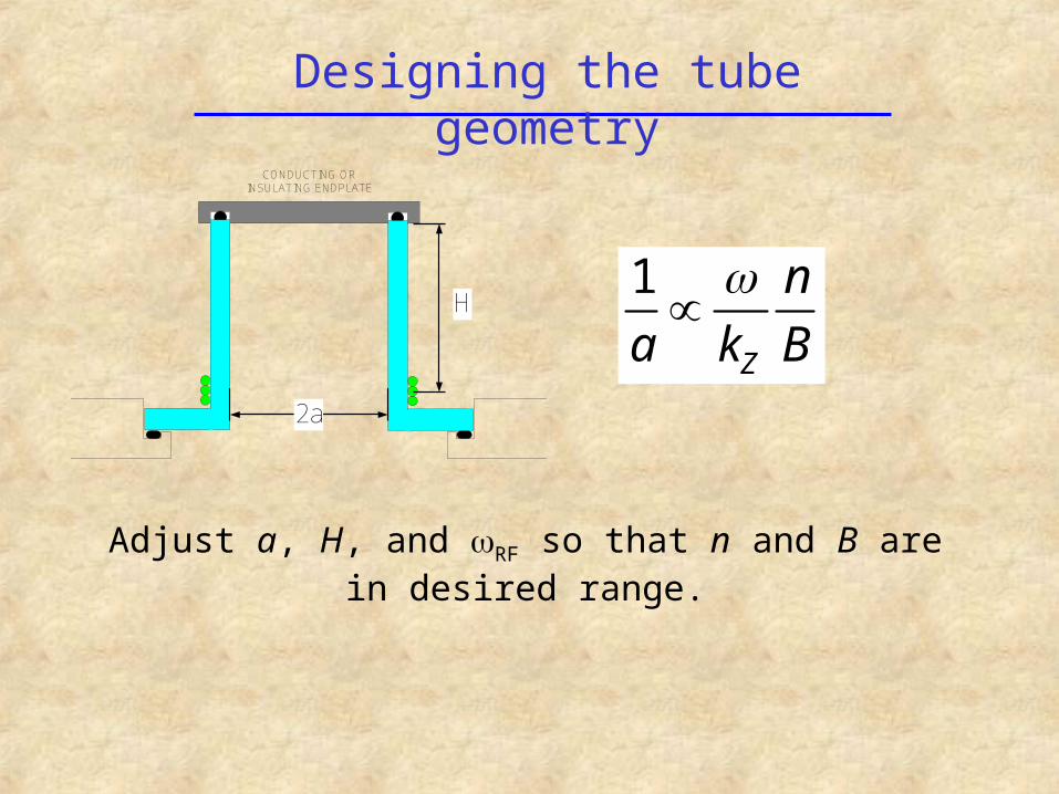
1

Z

n

a k B

Adjust a, H, and RF so that n and B are in desired range.

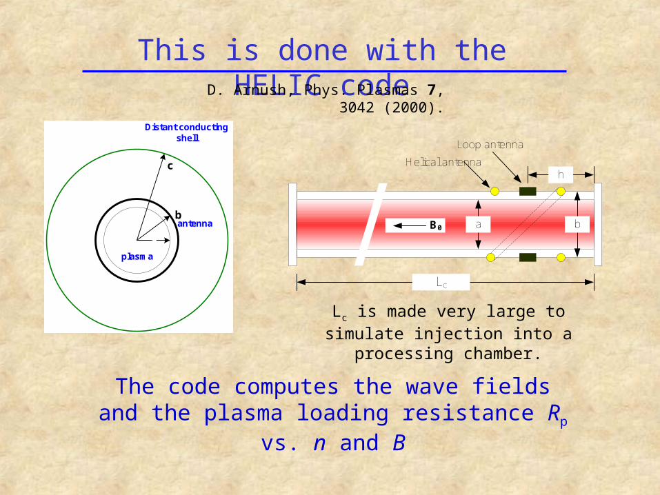
This is done with the HELIC codeD. Arnush, Phys. Plasmas 7, 3042 (2000).

a

b

c

Distant conducting shell

antenna

plasma

Lc

a b

h

Loop antenna

Helical antenna

B0

Lc is made very large to simulate injection into a processing chamber.

The code computes the wave fields and the plasma loading resistance Rp vs. n and B

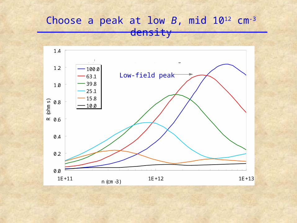
Choose a peak at low B, mid 1012 cm-3 density

0.0

0.2

0.4

0.6

0.8

1.0

1.2

1.4

1E+11 1E+12 1E+13n (cm-3)

R (

oh

ms)

100.0

63.1

39.8

25.1

15.8

10.0

B(G) L=2", 1mTorr, conducting

Low-field peak

0.0

0.5

1.0

1.5

2.0

2.5

1E+11 1E+12 1E+13n (cm-3)

R (

oh

ms)

1000

464

215

100

46

22

10

B (G) d = 3", H = 2", 13.56MHz

0.0

0.5

1.0

1.5

2.0

2.5

3.0

3.5

1E+11 1E+12 1E+13n (cm-3)

R (

oh

ms)

d = 4 in.

d = 3 in.

d = 2 in.

100G, H = 2", 13.56 MHzTube diameter

0.0

0.5

1.0

1.5

2.0

2.5

1E+11 1E+12 1E+13n (cm-3)

R (

oh

ms)

H = 3 in.

H = 2 in.

H = 1 in.

100G, d = 3", 13.56 MHz

0.0

0.5

1.0

1.5

2.0

2.5

3.0

3.5

1E+11 1E+12 1E+13n (cm-3)

R (

oh

ms)

f = 27.12 MHz

f = 13.56 MHz

f = 2 MHz

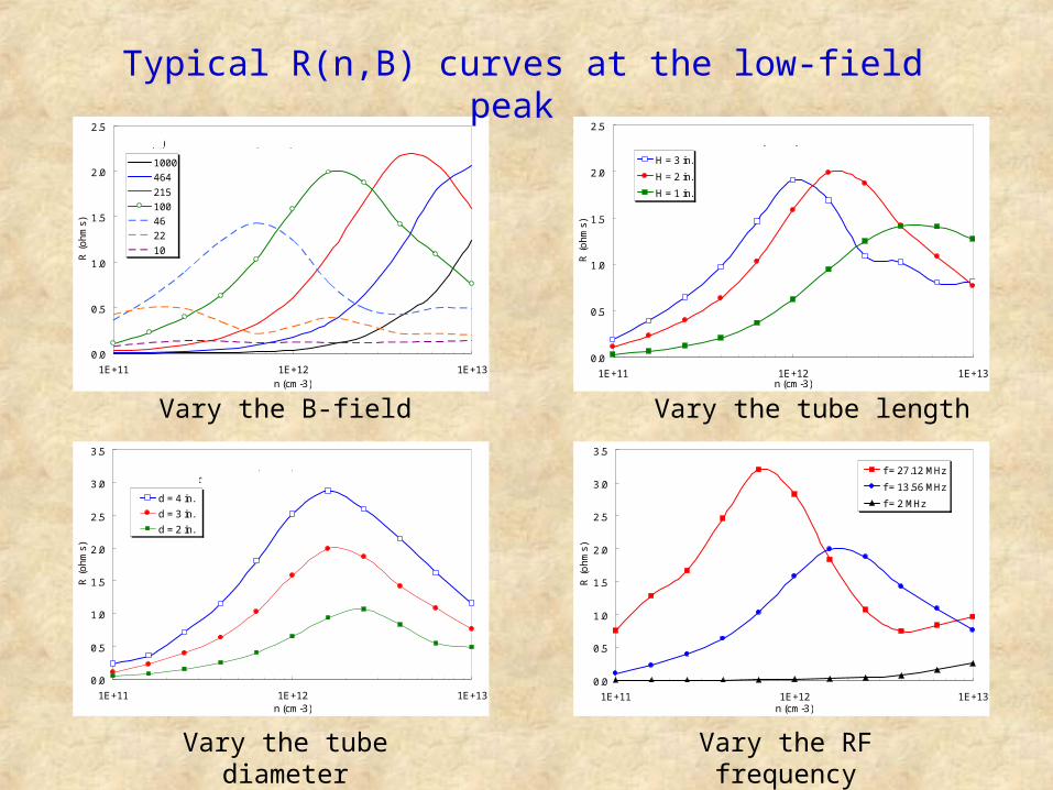
Typical R(n,B) curves at the low-field peak

Vary the B-field Vary the tube length

Vary the tube diameter Vary the RF frequency

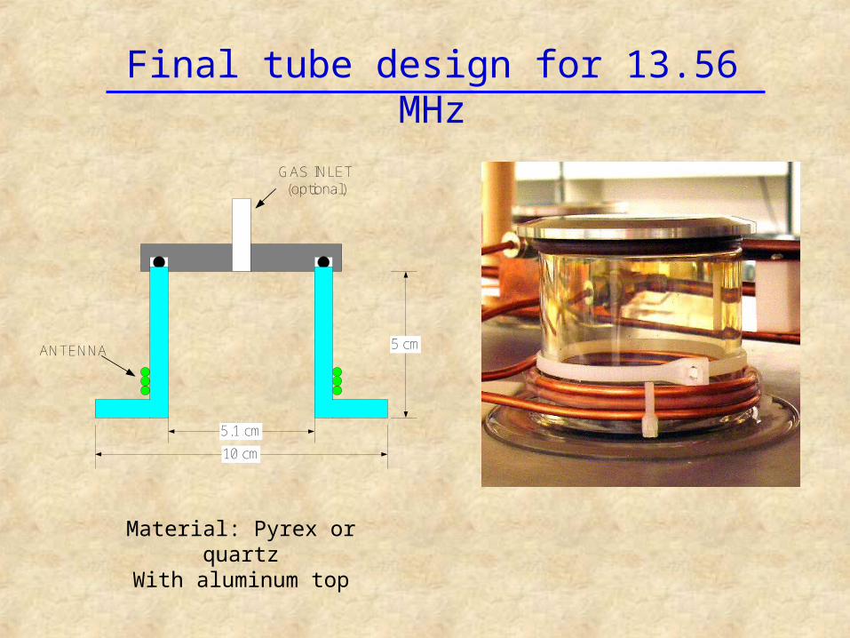
Final tube design for 13.56 MHz

5.1 cm

10 cm

5 cmANTENNA

GAS INLET (optional)

Material: Pyrex or quartzWith aluminum top

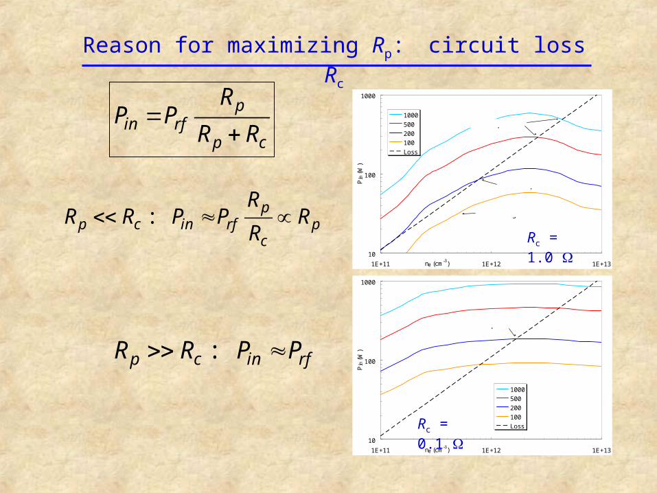
Reason for maximizing Rp: circuit loss Rc

pin rf

p c

RP P

R R

: pp c in rf p

c

RR R P P R

R

:p c in rfR R P P

10

100

1000

1E+11 1E+12 1E+13n0 (cm-3)

Pin

(W

)

1000

500

200

100

Loss

Prf (W)

No helicon ignition

Unstable equilibrium

Stable equilibrium

Rc = 1.0

10

100

1000

1E+11 1E+12 1E+13n0 (cm-3)

Pin

(W

)

1000

500

200

100

Loss

Prf (W)

Stable equilibria

Rc = 0.1

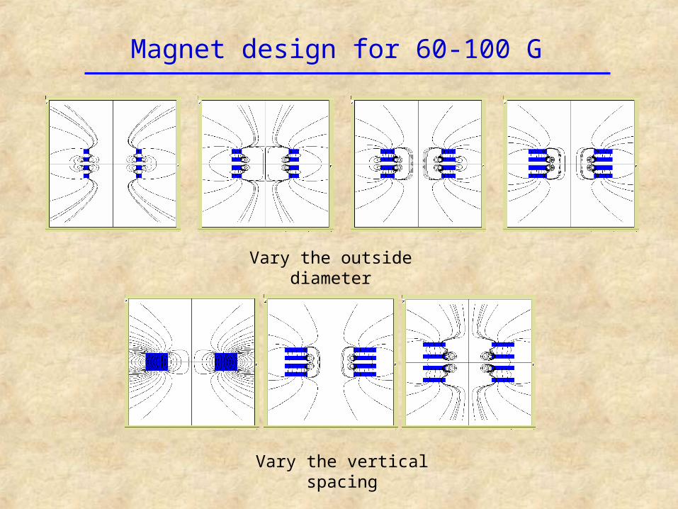
Magnet design for 60-100 G

Vary the outside diameter

Vary the vertical spacing

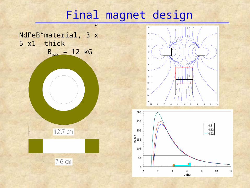
Final magnet design

12.7 cm

7.6 cm

PLASMA

NdFeB material, 3”x 5”x1” thickBmax = 12 kG

-16

-14

-12

-10

-8

-6

-4

-2

0

2

4

6

8

-10 -8 -6 -4 -2 0 2 4 6 8 10

0

50

100

150

200

250

300

0 2 4 6 8 10 12z (in.)

Bz (G

)

0.0

0.52

0.92

r (in.)

D

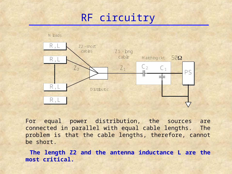
RF circuitry

R, L

R, L

R, L

R, L

PS

N loads

Z2 - short cables

Distributor

Z1Z2

Z1 - long cable

C1C2

Matching ckt. 50

For equal power distribution, the sources are connected in parallel with equal cable lengths. The problem is that the cable lengths, therefore, cannot be short.

The length Z2 and the antenna inductance L are the most critical.

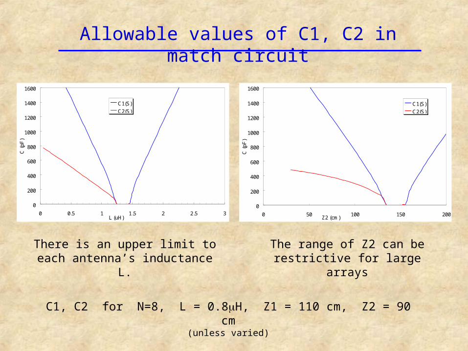
C1, C2 for N=8, L = 0.8H, Z1 = 110 cm, Z2 = 90 cm(unless varied)

0

200

400

600

800

1000

1200

1400

1600

0 50 100 150 200Z2 (cm)

C (

pF)

C1(S)

C2(S)

0

200

400

600

800

1000

1200

1400

1600

0 0.5 1 1.5 2 2.5 3L (uH)

C (

pF)

C1(S)

C2(S)

Allowable values of C1, C2 in match circuit

There is an upper limit to each antenna’s inductance L.

The range of Z2 can be restrictive for large arrays

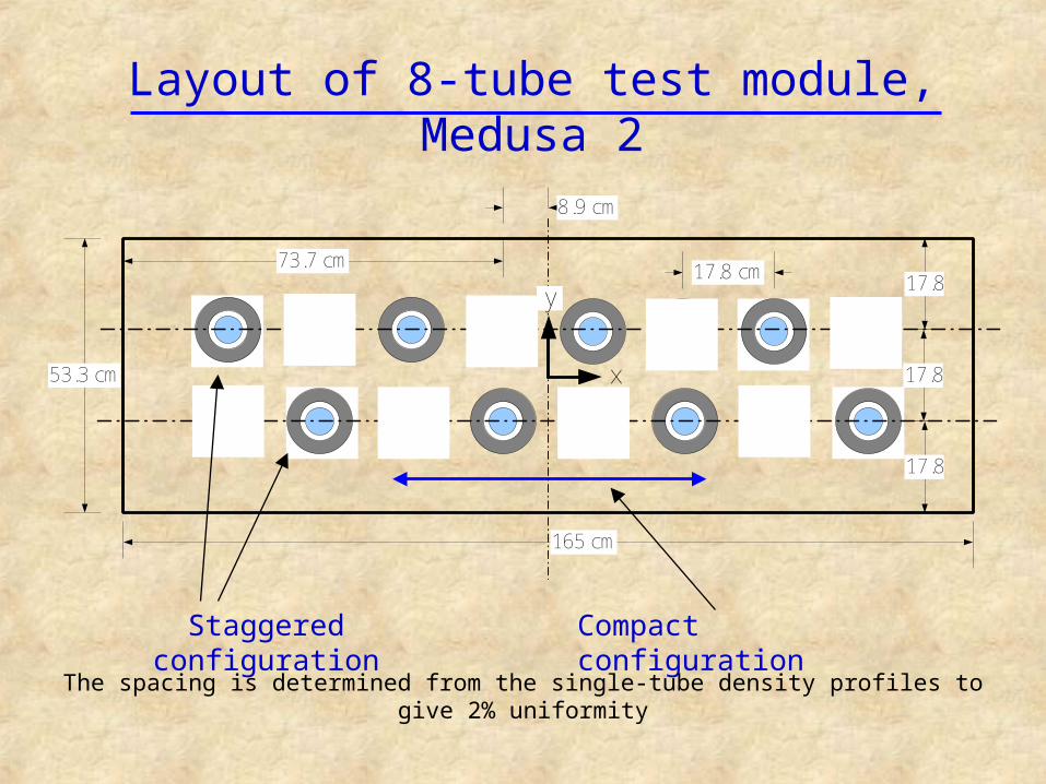
Layout of 8-tube test module, Medusa 2

165 cm

53.3 cm

17.8

17.8

17.8

17.8 cm73.7 cm

8.9 cm

x

y

Compact configurationStaggered configuration

The spacing is determined from the single-tube density profiles to give 2% uniformity

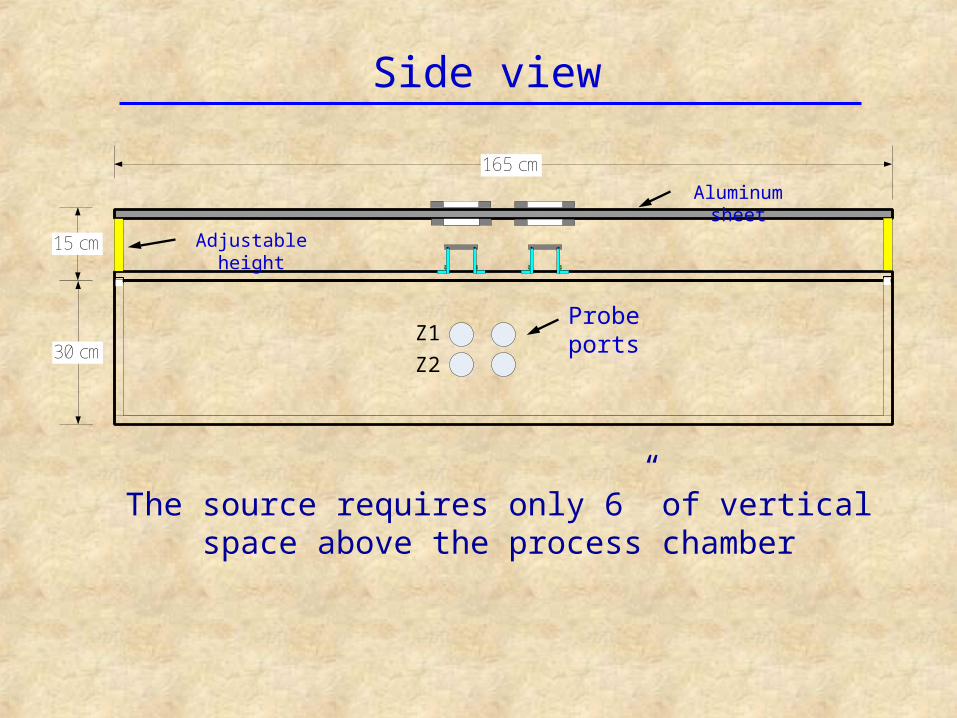
Side view

165 cm

30 cm

15 cm

Probe ports

Aluminum sheet

Adjustable height

The source requires only 6” of vertical space above the process chamber

Z1

Z2

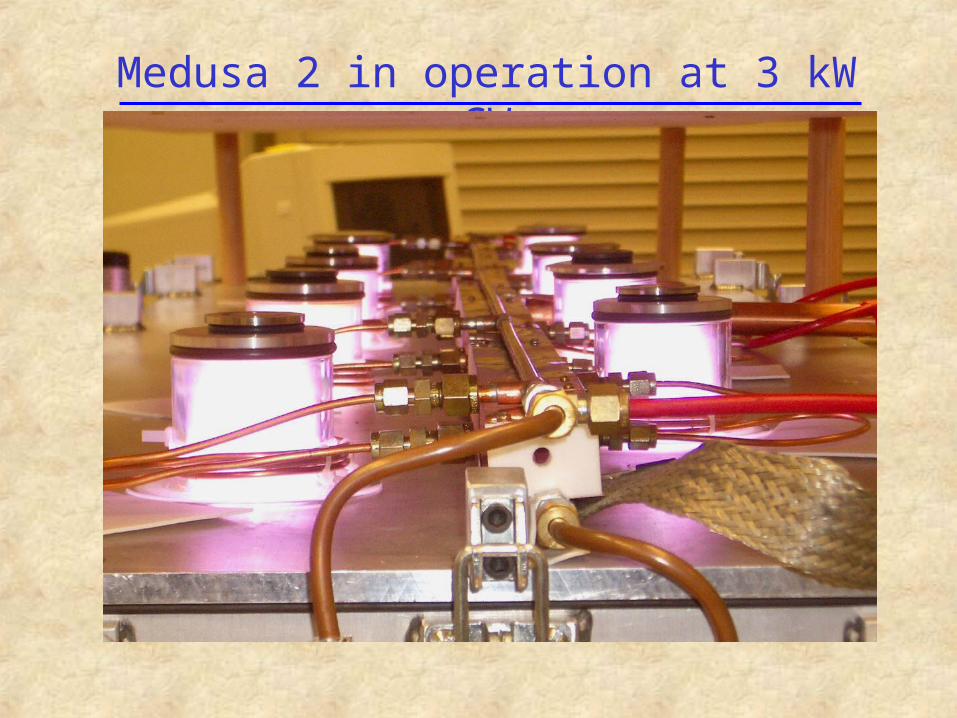
Medusa 2 in operation at 3 kW CW

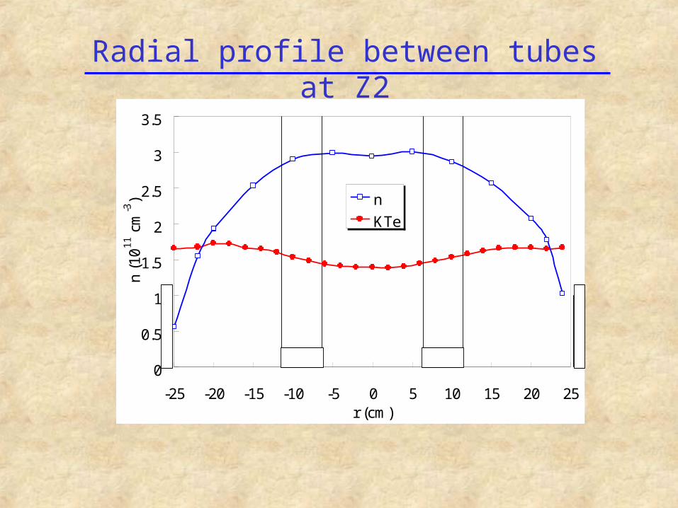
Radial profile between tubes at Z2

0

0.5

1

1.5

2

2.5

3

3.5

-25 -20 -15 -10 -5 0 5 10 15 20 25r (cm)

n (1

01

1 c

m-3

) n

KTe

UCLA

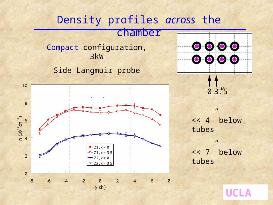
0 3.5”

Compact configuration, 3kW

Side Langmuir probe

Density profiles across the chamber

<< 4” below tubes

<< 7” below tubes

0

2

4

6

8

10

-8 -6 -4 -2 0 2 4 6 8y (in)

n (1

01

1cm

-3)

Z1, x = 0

Z1, x = 3.5

Z2, x = 0

Z2, x = 3.5

Compact 3kW, D=7", 20mTorr

UCLA

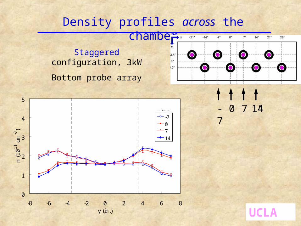
Density profiles across the chamber

0 7-7 14”

Staggered configuration, 3kW

Bottom probe array

0

1

2

3

4

5

-8 -6 -4 -2 0 2 4 6 8y (in.)

n (

10

11 c

m-3

)

-7

07

14

x (in.)Staggered3kW, D=7",

20mTorr

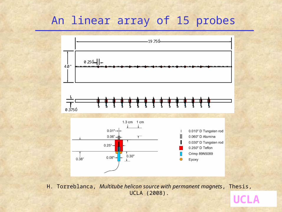
An linear array of 15 probes

UCLA

0.375Ó

19.75Ó

4.0"0.25Ó

H. Torreblanca, Multitube helicon source with permanent magnets, Thesis, UCLA (2008).

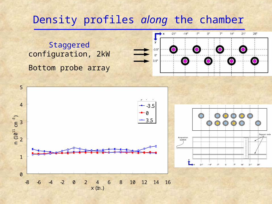
Density profiles along the chamber

Staggered configuration, 2kW

Bottom probe array

0

1

2

3

4

5

-8 -6 -4 -2 0 2 4 6 8 10 12 14 16x (in.)

n (1

011 c

m-3

)

-3.5

0

3.5

Staggered, 2kW, D=7", 20mTorr

y (in.)

UCLA

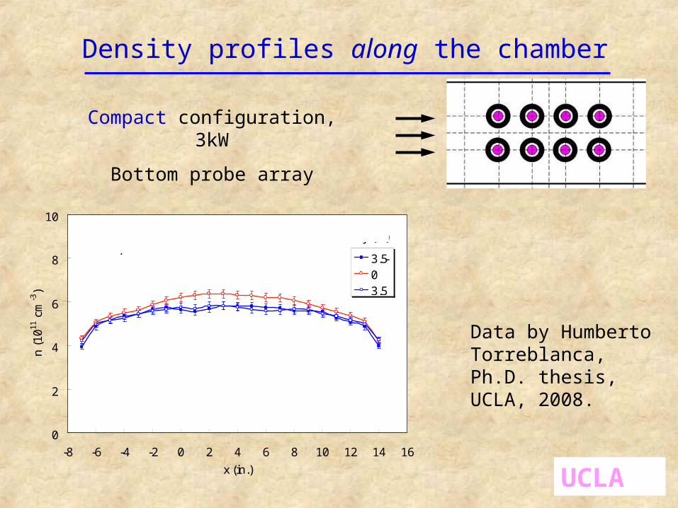
Density profiles along the chamber

Compact configuration, 3kW

Bottom probe array

0

2

4

6

8

10

-8 -6 -4 -2 0 2 4 6 8 10 12 14 16

x (in.)

n (

10

11 c

m-3

)

3.5-03.5

Compact, 3kW, D=7", 20mTorr

y (in)

Data by Humberto Torreblanca, Ph.D. thesis, UCLA, 2008.

Application to light gases,

like hydrogen

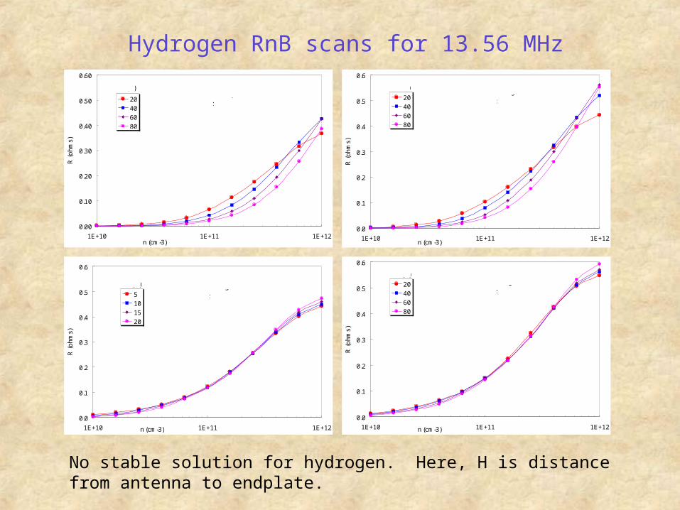
Hydrogen RnB scans for 13.56 MHz

0.00

0.10

0.20

0.30

0.40

0.50

0.60

1E+10 1E+11 1E+12n (cm-3)

R (

oh

ms)

20

40

60

80

B (G)H = 1.0 in. conducting

13.56 MHz

0.0

0.1

0.2

0.3

0.4

0.5

0.6

1E+10 1E+11 1E+12n (cm-3)

R (

oh

ms)

20

40

60

80

B (G)H = 1.5 in. conducting

13.56 MHz

0.0

0.1

0.2

0.3

0.4

0.5

0.6

1E+10 1E+11 1E+12n (cm-3)

R (

oh

ms)

20

40

60

80

H = 1.5 in. insulatingB (G)

13.56 MHz

0.0

0.1

0.2

0.3

0.4

0.5

0.6

1E+10 1E+11 1E+12n (cm-3)

R (

oh

ms)

5

10

15

20

B (G) H = 2.0 in. conducting

13.56 MHz

No stable solution for hydrogen. Here, H is distance from antenna to endplate.

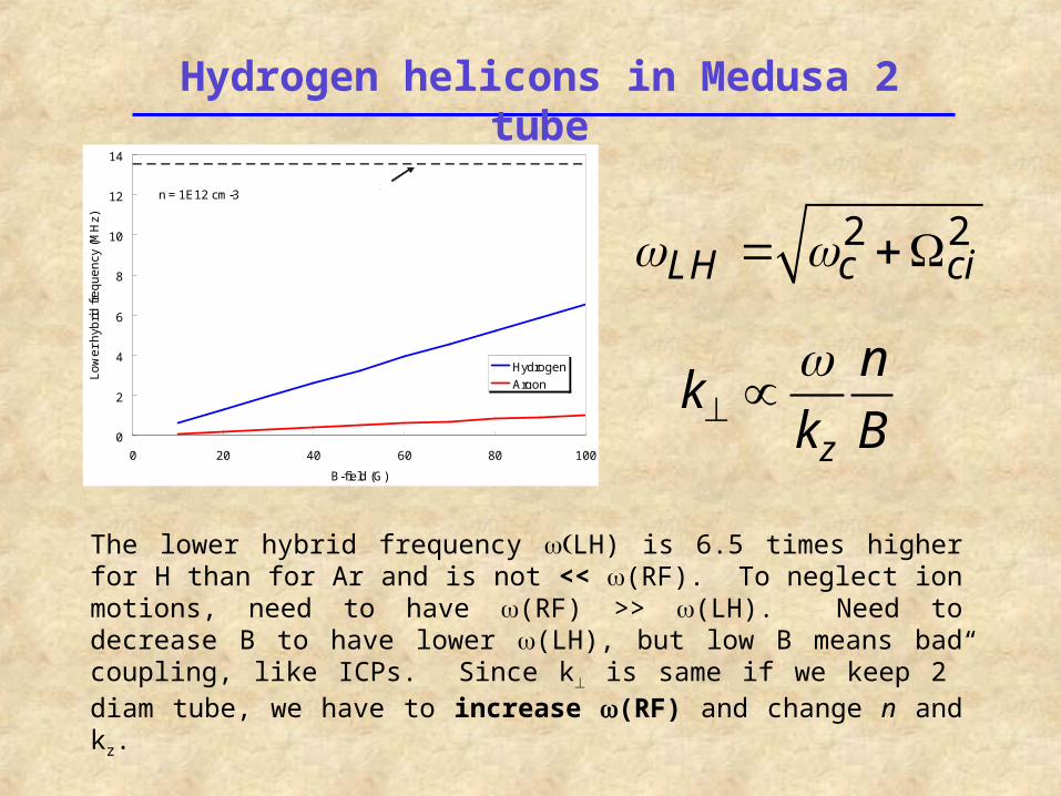
Hydrogen helicons in Medusa 2 tube

0

2

4

6

8

10

12

14

0 20 40 60 80 100

B-field (G)

Lo

we

r h

ybrid

fre

qu

en

cy (

MH

z)

Hydrogen

Argon

13.56 MHzn = 1E12 cm-3

z

nk

k B

The lower hybrid frequency LH) is 6.5 times higher for H than for Ar and is not << (RF). To neglect ion motions, need to have (RF) >> (LH). Need to decrease B to have lower (LH), but low B means bad coupling, like ICPs. Since k is same if we keep 2” diam tube, we have to increase (RF) and change n and kz.

2 2LH c ci

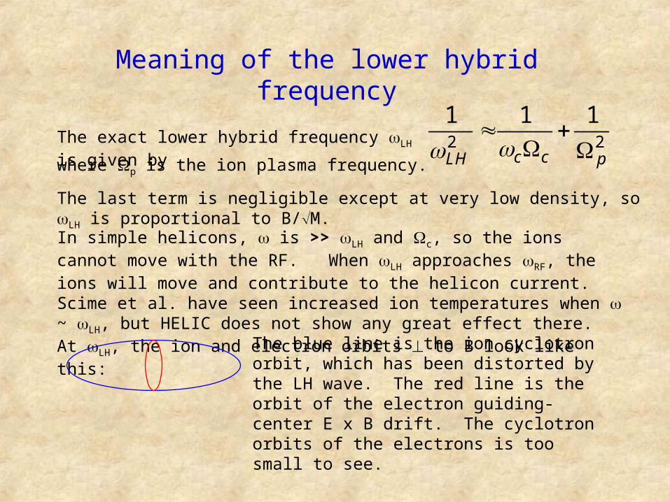
Meaning of the lower hybrid frequency

The exact lower hybrid frequency LH is given by

where p is the ion plasma frequency.

The last term is negligible except at very low density, so LH is proportional to B/M.

In simple helicons, is >> LH and c, so the ions cannot move with the RF. When LH approaches RF, the ions will move and contribute to the helicon current. Scime et al. have seen increased ion temperatures when ~ LH, but HELIC does not show any great effect there. At LH, the ion and electron orbits to B look like this:

The blue line is the ion cyclotron orbit, which has been distorted by the LH wave. The red line is the orbit of the electron guiding-center E x B drift. The cyclotron orbits of the electrons is too small to see.

2 2

1 1 1

c cLH p

0.0

0.2

0.4

0.6

0.8

1.0

1.2

1E+11 1E+12 1E+13n (cm-3)

R (

oh

ms)

10

30

50

70

90

H = 1.0" conductingB (G)

27.12 MHz

0.0

0.2

0.4

0.6

0.8

1.0

1.2

1E+11 1E+12 1E+13n (cm-3)

R (

oh

ms)

20

40

60

80

H = 1.5" conducting

B (G)

27.12 MHz

0.0

0.2

0.4

0.6

0.8

1.0

1.2

1E+11 1E+12 1E+13n (cm-3)

R (

oh

ms)

20

40

60

80

B (G)

H = 1.5 in. insulating

27.12 MHz

0.0

0.2

0.4

0.6

0.8

1.0

1.2

1E+11 1E+12 1E+13n (cm-3)

R (

oh

ms)

20

40

60

80

100

H = 3.0 in. conducting27.12 MHz

B (G)

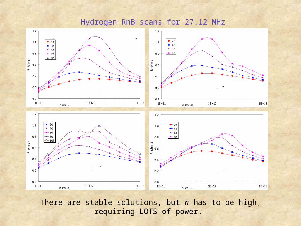
There are stable solutions, but n has to be high, requiring LOTS of power.

Hydrogen RnB scans for 27.12 MHz

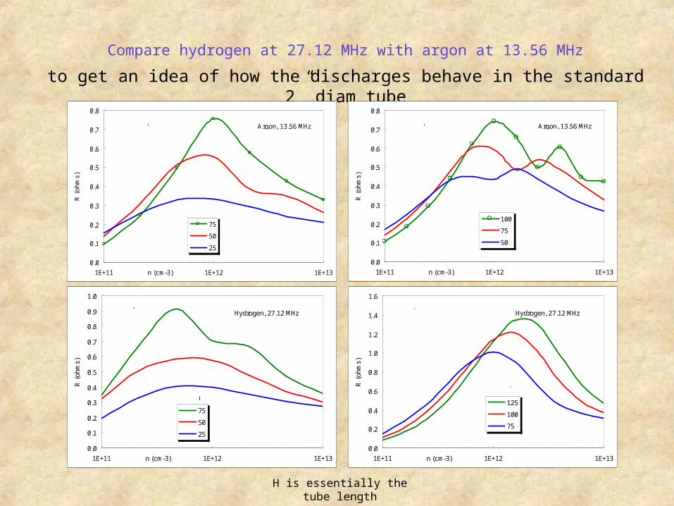
Compare hydrogen at 27.12 MHz with argon at 13.56 MHz

to get an idea of how the discharges behave in the standard 2” diam tube

0.0

0.1

0.2

0.3

0.4

0.5

0.6

0.7

0.8

1E+11 1E+12 1E+13n (cm-3)

R (

ohm

s)

75

50

25

Argon, 13.56 MHzH = 2"

B (G)

0.0

0.1

0.2

0.3

0.4

0.5

0.6

0.7

0.8

0.9

1.0

1E+11 1E+12 1E+13n (cm-3)

R (

ohm

s)

75

50

25

Hydrogen, 27.12 MHzH = 2"

B (G)

0.0

0.1

0.2

0.3

0.4

0.5

0.6

0.7

0.8

1E+11 1E+12 1E+13n (cm-3)

R (

ohm

s)

100

75

50

Argon, 13.56 MHzH = 3"

B (G)

0.0

0.2

0.4

0.6

0.8

1.0

1.2

1.4

1.6

1E+11 1E+12 1E+13n (cm-3)

R (

ohm

s)

125

100

75

Hydrogen, 27.12 MHzH = 3"

B (G)

H is essentially the tube length

0.0

0.1

0.2

0.3

0.4

0.5

0.6

0.7

0.8

0.9

1.0

1E+11 1E+12 1E+13n (cm-3)

R (

ohm

s)

100

80

60

40

20

Argon, 13.56 MHzB (G)

0

1000

2000

3000

4000

0.000 0.005 0.010 0.015 0.020 0.025r (m)

P(r

) (a

rb.)

100G, 1.6E1240 G, 6.3E11

Argon @ 13.56 MHz

0

1

2

3

4

-1.00 -0.95 -0.90 -0.85z(m)

P(z

) (a

rb.)

100G, 1.6E12

40 G, 6.3E11

Argon @ 13.56

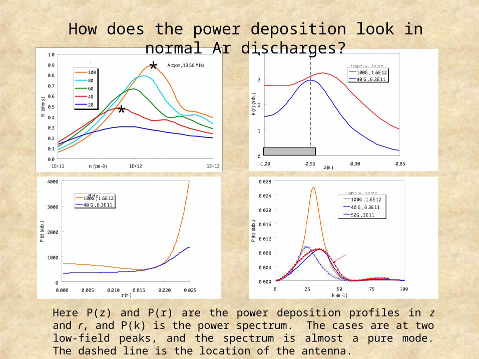
How does the power deposition look in normal Ar discharges?

Here P(z) and P(r) are the power deposition profiles in z and r, and P(k) is the power spectrum. The cases are at two low-field peaks, and the spectrum is almost a pure mode. The dashed line is the location of the antenna.

0.000

0.004

0.008

0.012

0.016

0.020

0.024

0.028

0 25 50 75 100k (m-1)

P(k

) (a

rb.)

100G, 1.6E12

40 G, 6.3E11

50G, 3E11

Argon @ 13.56

Hydrogen, 50G, 3E11 @ 27.12 MHz

*

*

0

200

400

600

800

1000

1200

1400

0.000 0.005 0.010 0.015 0.020 0.025r (m)

P(r

) (a

rb.)

Hydrogen

ArgonR = 0.564R = 0.397

0

1

2

3

4

-1.00 -0.95 -0.90 -0.85z(m)

P(z

) (a

rb.)

Hydrogen

Argon

0.000

0.002

0.004

0.006

0.008

0.010

0 20 40 60 80 100k(m-1)

P(k

) (a

rb.)

Argon

Hydrogen

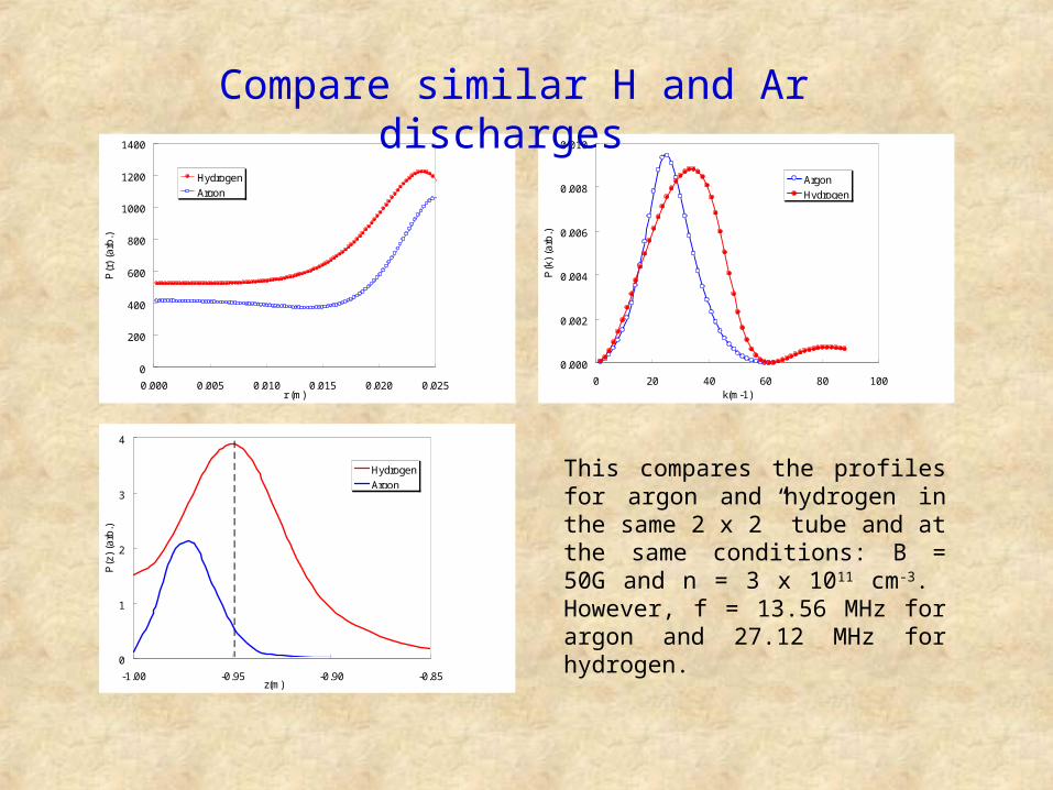
This compares the profiles for argon and hydrogen in the same 2 x 2” tube and at the same conditions: B = 50G and n = 3 x 1011 cm-3. However, f = 13.56 MHz for argon and 27.12 MHz for hydrogen.

Compare similar H and Ar discharges

0

2000

4000

6000

8000

0 0.005 0.01 0.015 0.02 0.025r (m)

P(r

)

1.5", conduct.

3.5", insul.

140G, 1.3E12H (in.), endplate

0

0.01

0.02

0.03

0.04

0.05

0 20 40 60 80 100 120 140k (m-1)

P(k

)

1.5", conduct.

3.5", insul.

140G, 1.3E12 H (in.), endplate

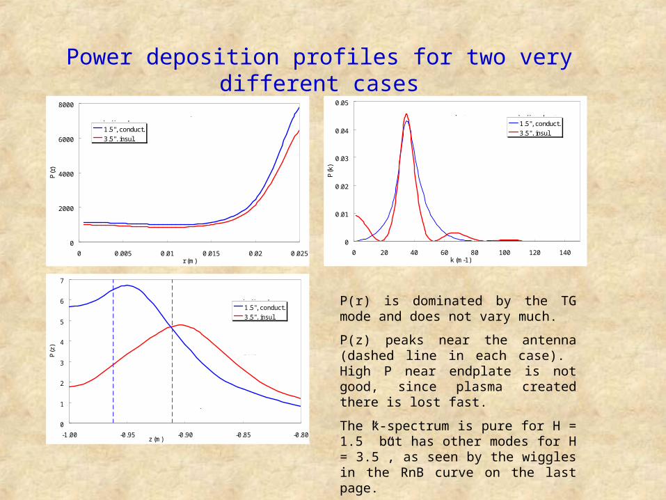
Both are near density peak, but conducting case has pure mode.

Power deposition profiles for two very different cases

P(r) is dominated by the TG mode and does not vary much.

P(z) peaks near the antenna (dashed line in each case). High P near endplate is not good, since plasma created there is lost fast.

The k-spectrum is pure for H = 1.5” but has other modes for H = 3.5”, as seen by the wiggles in the RnB curve on the last page.0

1

2

3

4

5

6

7

-1.00 -0.95 -0.90 -0.85 -0.80z (m)

P(z

)

1.5", conduct.

3.5", insul.

140G, 1.3E12

H (in.), endplate

R = 1.41

R = 1.67

0

1

2

3

4

5

6

-1.00 -0.95 -0.90 -0.85 -0.80z (m)

|Ez|

(z)

H = 1.5"

H = 3"

140G, 1.4E12, conducting

R = 1.67

R = 0.87

140G, 1.3E12, conducting

0

1

2

3

4

5

6

7

-1.00 -0.95 -0.90 -0.85 -0.80z (m)

P(z

)

H = 1.5 in.

H = 3 in.

140G, 1.3E12, conducting

140G, 1.4E12, conducting R = 1.67

R = 0.87

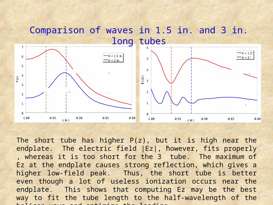
Comparison of waves in 1.5 in. and 3 in. long tubes

The short tube has higher P(z), but it is high near the endplate. The electric field |Ez|, however, fits properly , whereas it is too short for the 3” tube. The maximum of Ez at the endplate causes strong reflection, which gives a higher low-field peak. Thus, the short tube is better even though a lot of useless ionization occurs near the endplate. This shows that computing Ez may be the best way to fit the tube length to the half-wavelength of the helicon wave and optimize the loading.

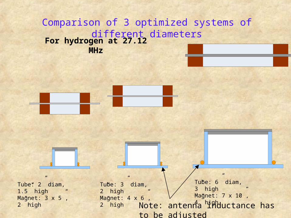
Comparison of 3 optimized systems of different diameters

For hydrogen at 27.12 MHz

Tube: 2” diam, 1.5” highMagnet: 3 x 5”, 2” high

Tube: 3” diam, 2” highMagnet: 4 x 6”, 2” high

Tube: 6” diam, 3” highMagnet: 7 x 10”, 4” high

Note: antenna inductance has to be adjusted

Application to

spacecraft thrusters

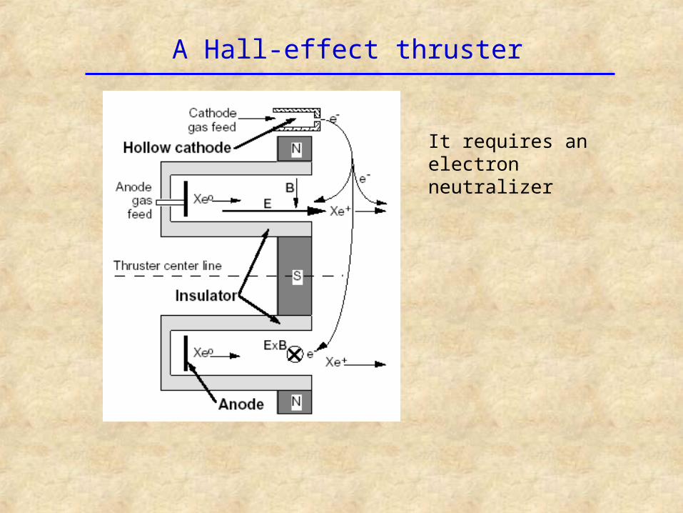
A Hall-effect thruster

It requires an electron neutralizer

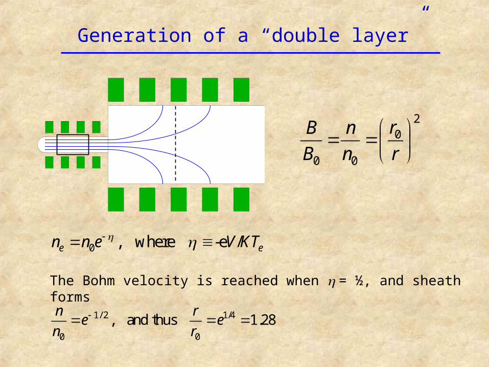
Generation of a “double layer”

20

0 0

rB n

B n r

0 , where -e /e en n e V KT

1/ 2 1/4

0 0

, and thus 1.28n r

e en r

The Bohm velocity is reached when = ½, and sheath forms

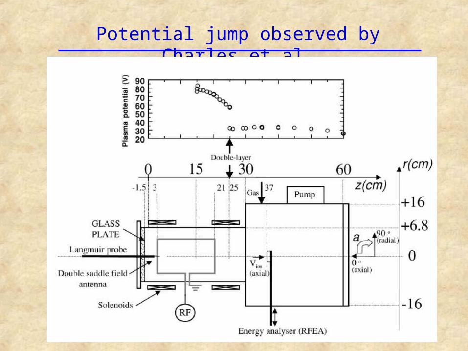
Potential jump observed by Charles et al.

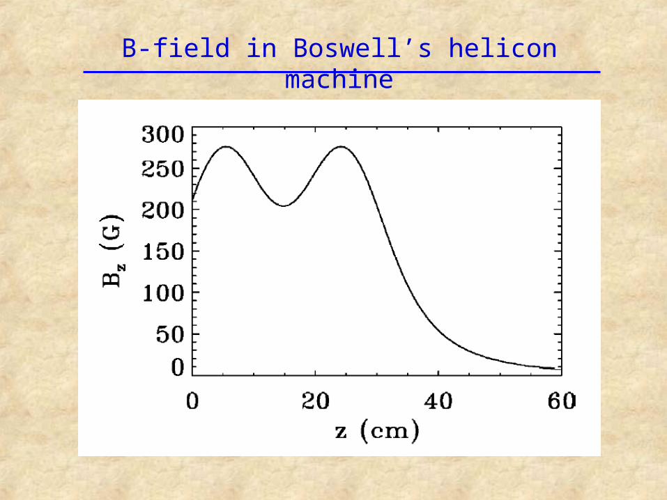
B-field in Boswell’s helicon machine

Medusa source adapted to VASIMR

9 11

5

D

16

The optimized 9-cm diam source is shown with dimensions in cm, together with a NdFeB magnet designed for 400G at the antenna. D is the distance from the midplane of the magnet to the midplane of the antenna. The magnet is made in two pieces supported by a non-ferrous metal plate. The B-field can be adjusted by changing D either by hand or remotely with a motor.

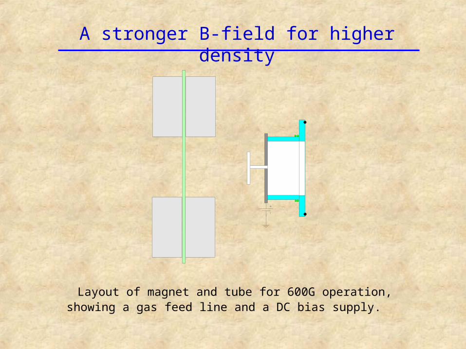
A stronger B-field for higher density

Layout of magnet and tube for 600G operation,showing a gas feed line and a DC bias supply.

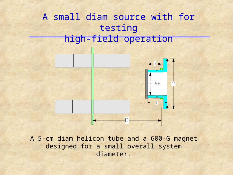
A small diam source with for testinghigh-field operation

5 11

3

D

6.6

L

A 5-cm diam helicon tube and a 600-G magnet designed for a small overall system diameter.

Conclusion on spacecraft thrusters

• “Ambipolar” sources can eject ions with automatic space-charge neutralization.

• Helicon sources can generate ions efficiently.

• Permanent magnets can reduce the complexity of helicon sources.

• However, for the fields and densities considered for the VASIMR project, the magnet may be too large to be practical.