APPLICATIONS OF DIFFERENTIATION 4. 4.1 Maximum and Minimum Values In this section, we will learn: How to find the maximum and minimum values of a function.

APPLICATIONS OF DIFFERENTIATIONAPPLICATIONS OF DIFFERENTIATION

4

4.1Maximum and

Minimum Values

In this section, we will learn:

How to find the maximum

and minimum values of a function.

APPLICATIONS OF DIFFERENTIATION

MAXIMUM & MINIMUM VALUES

A function f has an absolute maximum

(or global maximum) at c if f(c) ≥ f(x) for

all x in D, where D is the domain of f.

The number f(c) is called the maximum value

of f on D.

Definition 1


Similarly, f has an absolute minimum at c

if f(c) ≤ f(x) for all x in D and the number f(c)

is called the minimum value of f on D.

The maximum and minimum values of f

are called the extreme values of f.

Definition 1


The figure shows the graph of a function f

with absolute maximum at d and absolute

minimum at a.

Note that (d, f(d)) is the highest point on the graph and (a, f(a)) is the lowest point.

Figure 4.1.1, p. 205

LOCAL MAXIMUM VALUE

If we consider only values of x near b—for

instance, if we restrict our attention to the

interval (a, c)—then f(b) is the largest of those

values of f(x).

It is called a local maximum value of f.

Figure 4.1.1, p. 205

Likewise, f(c) is called a local minimum value

of f because f(c) ≤ f(x) for x near c—for

instance, in the interval (b, d).

The function f also has a local minimum at e.

LOCAL MINIMUM VALUE

Figure 4.1.1, p. 205


In general, we have the following definition.

A function f has a local maximum (or relative

maximum) at c if f(c) ≥ f(x) when x is near c.

This means that f(c) ≥ f(x) for all x in some open interval containing c.

Similarly, f has a local minimum at c if f(c) ≤

f(x)

when x is near c.

Definition 2


The function f(x) = cos x takes on its (local

and absolute) maximum value of 1 infinitely

many times—since cos 2nπ = 1 for any

integer n and -1 ≤ cos x ≤ 1 for all x.

Likewise, cos (2n + 1)π = -1 is its minimum

value—where n is any integer.

Example 1


If f(x) = x2, then f(x) ≥ f(0) because

x2 ≥ 0 for all x.

Therefore, f(0) = 0 is the absolute (and local) minimum value of f.

Example 2


This corresponds to the fact that the origin

is the lowest point on the parabola y = x2.

However, there is no highest point on the parabola. So, this function has no maximum value.

Example 2

Figure 4.1.2, p. 205


From the graph of the function f(x) = x3,

we see that this function has neither

an absolute maximum value nor an absolute

minimum value.

In fact, it has no localextreme values either.

Example 3

Figure 4.1.3, p. 205


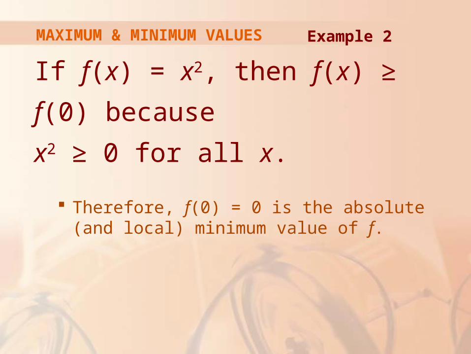
The graph of the function

f(x) = 3x4 – 16x3 + 18x2 -1 ≤ x ≤ 4

is shown here.

Example 4

Figure 4.1.4, p. 206


You can see that f(1) = 5 is a local

maximum, whereas the absolute maximum

is f(-1) = 37.

This absolute maximum is not a local maximum because it occurs at an endpoint.

Example 4

Figure 4.1.4, p. 206


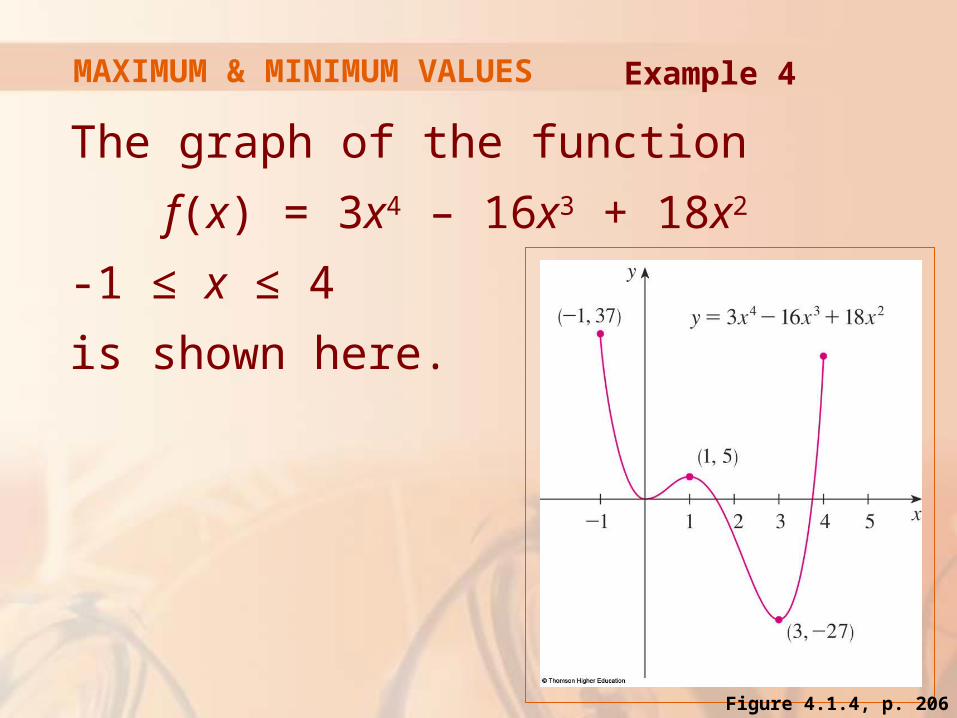
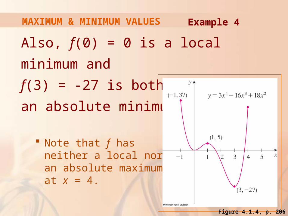
Also, f(0) = 0 is a local minimum and

f(3) = -27 is both a local and an absolute

minimum.

Note that f has neither a local nor an absolute maximumat x = 4.

Example 4

Figure 4.1.4, p. 206


We have seen that some functions have

extreme values, whereas others do not.

The following theorem gives conditions

under which a function is guaranteed to

possess extreme values.

EXTREME VALUE THEOREM

If f is continuous on a closed interval [a, b],

then f attains an absolute maximum value f(c)

and an absolute minimum value f(d) at some

numbers c and d in [a, b].

Theorem 3

The theorem is illustrated

in the figures.

Note that an extreme value can be taken on more than once.


Figure 4.1.5, p. 206

Although the theorem is intuitively

very plausible, it is difficult to prove

and so we omit the proof.


The figures show that a function need not

possess extreme values if either hypothesis

(continuity or closed interval) is omitted from

the theorem.


Figure 4.1.6, p. 206 Figure 4.1.7, p. 206

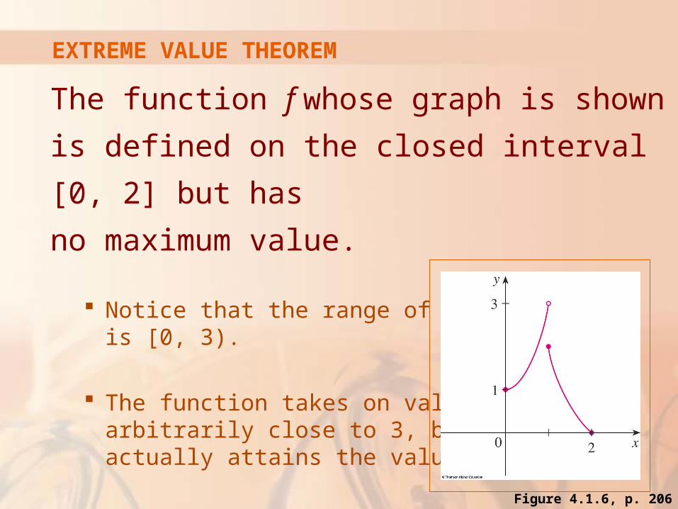
The function f whose graph is shown is

defined on the closed interval [0, 2] but has

no maximum value.

Notice that the range of f is [0, 3).

The function takes on values arbitrarily close to 3, but never actually attains the value 3.


Figure 4.1.6, p. 206

This does not contradict the theorem

because f is not continuous.

Nonetheless, a discontinuous function could have maximum and minimum values.


Figure 4.1.6, p. 206

The function g shown here is continuous

on the open interval (0, 2) but has neither

a maximum nor a minimum value.

The range of g is (1, ∞). The function takes on

arbitrarily large values. This does not contradict

the theorem because the interval (0, 2) is not closed.


Figure 4.1.7, p. 206

The theorem says that a continuous function

on a closed interval has a maximum value

and a minimum value.

However, it does not tell us how to find these

extreme values. We start by looking for local extreme values.


LOCAL EXTREME VALUES

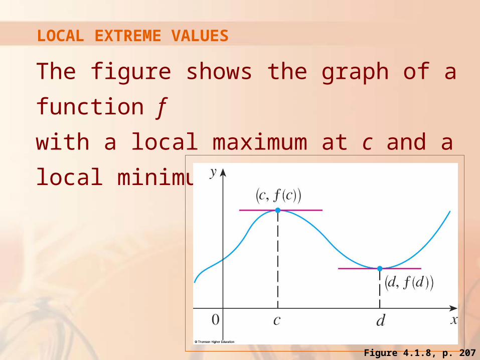
The figure shows the graph of a function f

with a local maximum at c and a local

minimum at d.

Figure 4.1.8, p. 207

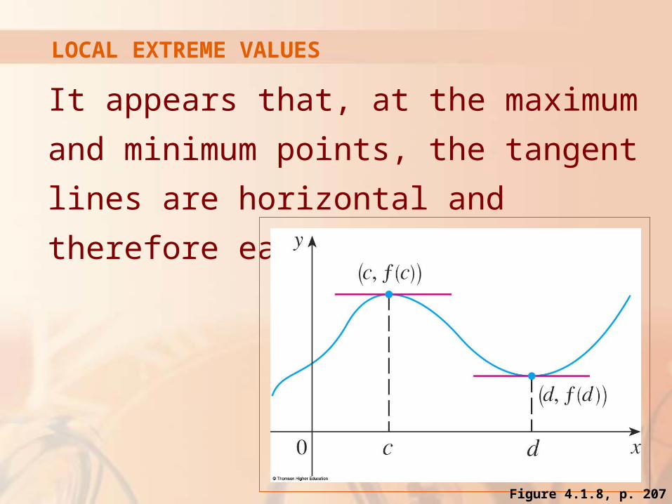
It appears that, at the maximum and

minimum points, the tangent lines are

horizontal and therefore each has slope 0.


Figure 4.1.8, p. 207

We know that the derivative is the slope

of the tangent line. So, it appears that f ’(c) = 0 and f ’(d) = 0.


Figure 4.1.8, p. 207

The following theorem says that

this is always true for differentiable

functions.


FERMAT’S THEOREM

If f has a local maximum or

minimum at c, and if f ’(c) exists, then

f ’(c) = 0.

Theorem 4

Suppose, for the sake of definiteness, that f

has a local maximum at c.

Then, according to Definition 2, f(c) ≥ f(x)

if x is sufficiently close to c.

ProofFERMAT’S THEOREM

This implies that, if h is sufficiently close to 0,

with h being positive or negative, then

f(c) ≥ f(c + h)

and therefore

f(c + h) – f(c) ≤ 0

Proof (Equation 5)FERMAT’S THEOREM

We can divide both sides of an inequality

by a positive number.

Thus, if h > 0 and h is sufficiently small, we have:

( ) ( )0

f c h f c

h


Taking the right-hand limit of both sides

of this inequality (using Theorem 2 in

Section 2.3), we get:

0 0

( ) ( )lim lim 0 0h h

f c h f c

h


However, since f ’(c) exists,

we have:

So, we have shown that f ’(c) ≤ 0.

0

0

( ) ( )'( ) lim

( ) ( )lim

h

h

f c h f cf c

hf c h f c

h


If h < 0, then the direction of the inequality

in Equation 5 is reversed when we divide by

h:

( ) ( )0 0

f c h f ch

h


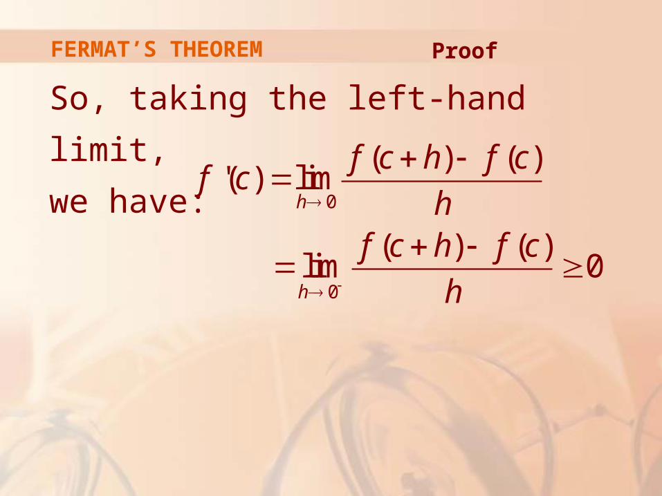
So, taking the left-hand limit,

we have:

0

0

( ) ( )'( ) lim

( ) ( )lim 0

h

h

f c h f cf c

hf c h f c

h


We have shown that f ’(c) ≥ 0 and also

that f ’(c) ≤ 0.

Since both these inequalities must be true,

the only possibility is that f ’(c) = 0.


We have proved the theorem for

the case of a local maximum.

The case of a local minimum can be proved in a similar manner.

Alternatively, we could use Exercise 76 to deduce it from the case we have just proved.

FERMAT’S THEOREM Proof

The following examples caution us

against reading too much into the theorem.

We can’t expect to locate extreme values simply by setting f ’(x) = 0 and solving for x.

FERMAT’S THEOREM

If f(x) = x3, then f ’(x) = 3x2, so f ’(0) = 0.

However, f has no maximum or minimum at 0—as you can see from the graph.

Alternatively, observe that x3 > 0 for x > 0 but x3 < 0 for x < 0.

Example 5FERMAT’S THEOREM

Figure 4.1.9, p. 208

The fact that f ’(0) = 0 simply means that

the curve y = x3 has a horizontal tangent

at (0, 0).

Instead of having a maximum or minimum at (0, 0), the curve crosses its horizontal tangent there.


Figure 4.1.9, p. 208

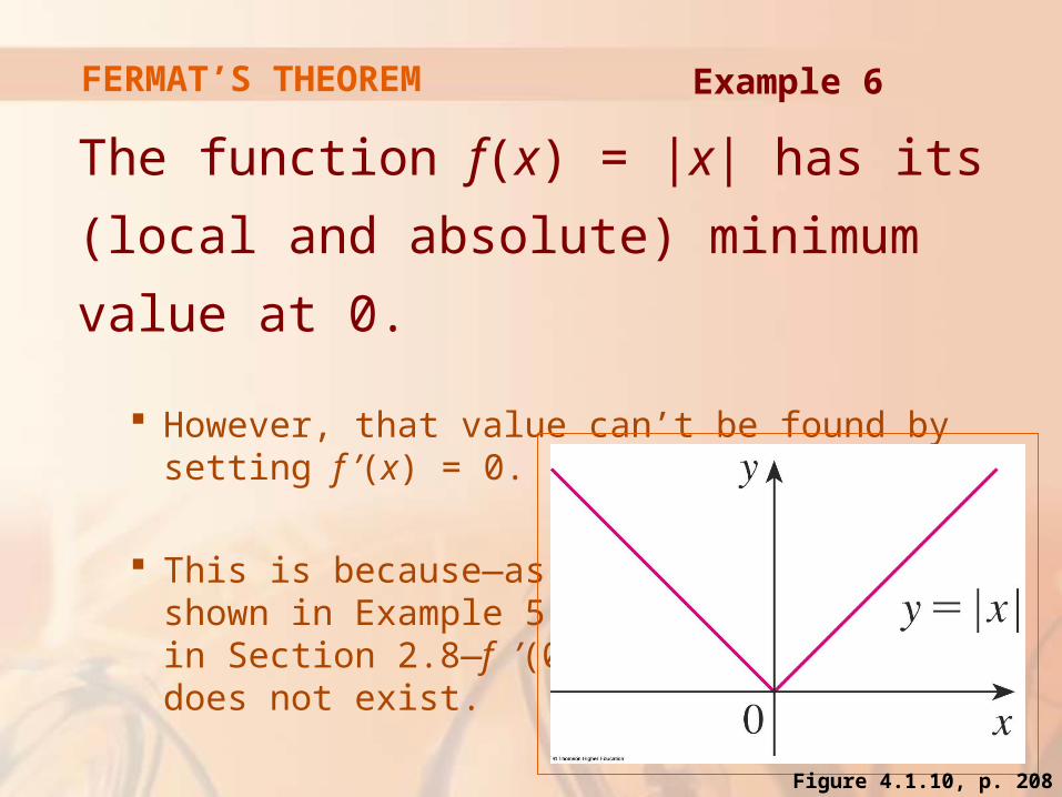
The function f(x) = |x| has its (local and

absolute) minimum value at 0.

However, that value can’t be found by setting f ’(x) = 0.

This is because—as shown in Example 5 in Section 2.8—f ’(0) does not exist.


Figure 4.1.10, p. 208

WARNING

Examples 5 and 6 show that we must

be careful when using the theorem.

Example 5 demonstrates that, even when f ’(c) = 0, there need not be a maximum or minimum at c.

In other words, the converse of the theorem is false in general.

Furthermore, there may be an extreme value even when f ’(c) does not exist (as in Example 6).

The theorem does suggest that we should

at least start looking for extreme values of f

at the numbers c where either:

f ’(c) = 0

f ’(c) does not exist

FERMAT’S THEOREM

Such numbers are given a

special name—critical numbers.

FERMAT’S THEOREM

CRITICAL NUMBERS

A critical number of a function f is

a number c in the domain of f such that

either f ’(c) = 0 or f ’(c) does not exist.

Definition 6

Find the critical numbers of

f(x) = x3/5(4 - x). The Product Rule gives:

3/5 2/535

3/52/5

2/5 2/5

'( ) ( 1) (4 )( )

3(4 )

55 3(4 ) 12 8

5 5

f x x x x

xx

xx x x

x x

Example 7CRITICAL NUMBERS

Figure 4.1.11, p. 208

The same result could be obtained by first writing f(x) = 4x3/5 – x8/5.

Therefore, f ’(x) = 0 if 12 – 8x = 0.

That is, x = , and f ’(x) does not exist when x = 0.

Thus, the critical numbers are and 0.

Example 7CRITICAL NUMBERS

32

32

In terms of critical numbers, Fermat’s

Theorem can be rephrased as follows

(compare Definition 6 with Theorem 4).

CRITICAL NUMBERS

If f has a local maximum or

minimum at c, then c is a critical

number of f.

CRITICAL NUMBERS Theorem 7

CLOSED INTERVALS

To find an absolute maximum or minimum

of a continuous function on a closed interval,

we note that either:

It is local (in which case, it occurs at a critical number by Theorem 7).

It occurs at an endpoint of the interval.

Therefore, the following

three-step procedure always

works.

CLOSED INTERVALS

CLOSED INTERVAL METHOD

To find the absolute maximum and minimum

values of a continuous function f on a closed

interval [a, b]:

1. Find the values of f at the critical numbers of f in (a, b).

2. Find the values of f at the endpoints of the interval.

3. The largest value from 1 and 2 is the absolute maximum value. The smallest is the absolute minimum value.


Find the absolute maximum

and minimum values of the function

f(x) = x3 – 3x2 + 1 -½ ≤ x ≤ 4

Example 8

As f is continuous on [-½, 4], we

can use the Closed Interval Method:

f(x) = x3 – 3x2 + 1

f ’(x) = 3x2 – 6x = 3x(x – 2)

CLOSED INTERVAL METHOD Example 8


As f ’(x) exists for all x, the only critical

numbers of f occur when f ’(x) = 0, that is,

x = 0 or x = 2.

Notice that each of these numbers lies in

the interval (-½, 4).

Example 8


The values of f at these critical numbers

are: f(0) = 1 f(2) = -3

The values of f at the endpoints of the interval

are: f(-½) = 1/8 f(4) = 17

Comparing these four numbers, we see that the absolute maximum value is f(4) = 17 and the absolute minimum value is f(2) = -3.

Example 8


Note that the absolute maximum occurs

at an endpoint, whereas the absolute

minimum occurs at a critical number.

Example 8


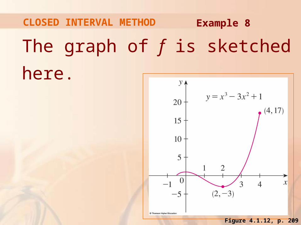
The graph of f is sketched here.

Example 8

Figure 4.1.12, p. 209

If you have a graphing calculator or

a computer with graphing software, it is

possible to estimate maximum and minimum

values very easily.

However, as the next example shows, calculus is needed to find the exact values.

EXACT VALUES

a.Use a graphing device to estimate

the absolute minimum and maximum values

of the function f(x) = x – 2 sin x, 0 ≤ x ≤ 2π.

b.Use calculus to find the exact minimum

and maximum values.

Example 9EXACT VALUES

The figure shows a graph of f in

the viewing rectangle [0, 2π] by [-1, 8].

Example 9 aEXACT VALUES

Figure 4.1.13, p. 209

By moving the cursor close to the maximum

point, we see the y-coordinates don’t change

very much in the vicinity of the maximum.

The absolute maximum value is about 6.97

It occurs when x ≈ 5.2


Figure 4.1.13, p. 209

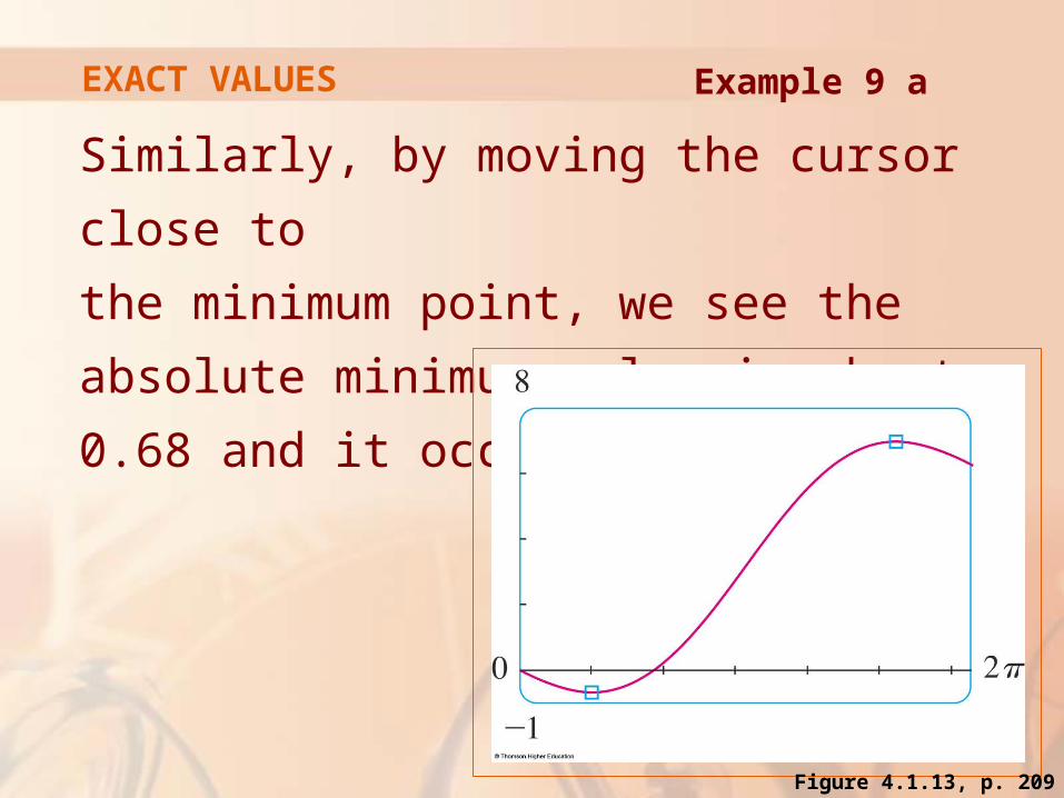
Similarly, by moving the cursor close to

the minimum point, we see the absolute

minimum value is about –0.68 and it occurs

when x ≈ 1.0


Figure 4.1.13, p. 209

It is possible to get more accurate

estimates by zooming in toward

the maximum and minimum points.

However, instead, let’s use calculus.


The function f(x) = x – 2 sin x is continuous

on [0, 2π].

As f ’(x) = 1 – 2 cos x, we have f ’(x) = 0

when cos x = ½. This occurs when x = π/3 or 5π/3.

Example 9 bEXACT VALUES

The values of f at these critical points

are

and

( / 3) 2sin 3 0.6848533 3 3

f


5 5 5(5 / 3) 2sin 3 6.968039

3 3 3f

The values of f at the endpoints

are

f(0) = 0

and

f(2π) = 2π ≈ 6.28


Comparing these four numbers and

using the Closed Interval Method, we see

the absolute minimum value is

f(π/3) = π/3 -

and the absolute maximum value is

f(5π/3) = 5π/3 +

The values from (a) serve as a check on our work.

3


3

The Hubble Space Telescope was

deployed on April 24, 1990, by the space

shuttle Discovery.

Example 10MAXIMUM & MINIMUM VALUES

A model for the velocity of the shuttle

during this mission—from liftoff at t = 0

until the solid rocket boosters were jettisoned

at t = 126 s—is given by:

v(t) = 0.001302t3 – 0.09029t2 + 23.61t – 3.083

(in feet per second)


Using this model, estimate the absolute

maximum and minimum values of

the acceleration of the shuttle between

liftoff and the jettisoning of the boosters.


We are asked for the extreme values

not of the given velocity function,

but rather of the acceleration function.


So, we first need to differentiate to find

the acceleration:

3 2

2

( ) '( )

(0.001302 0.09029

23.61 3.083)

0.003906 0.18058 23.61

a t v t

dt t

dtt

t t


We now apply the Closed Interval Method

to the continuous function a on the interval

0 ≤ t ≤ 126.

Its derivative is:

a’(t) = 0.007812t – 0.18058


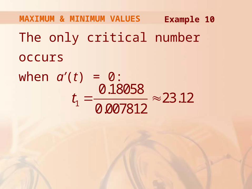
The only critical number occurs

when a’(t) = 0:

1

0.1805823.12

0.007812t


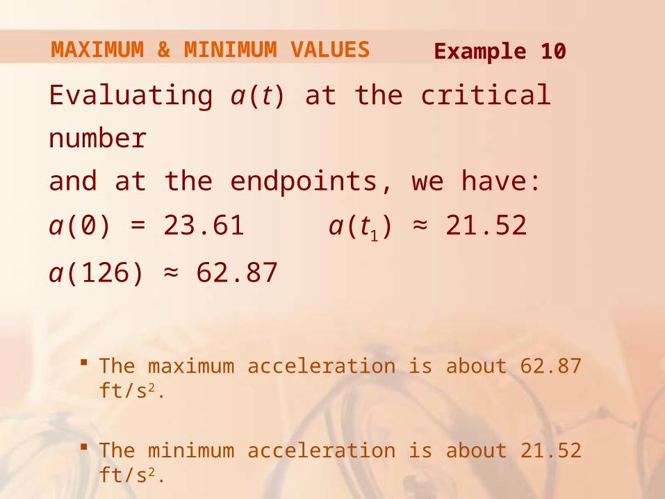
Evaluating a(t) at the critical number

and at the endpoints, we have:

a(0) = 23.61 a(t1) ≈ 21.52 a(126) ≈ 62.87

The maximum acceleration is about 62.87 ft/s2.

The minimum acceleration is about 21.52 ft/s2.


APPLICATIONS OF DIFFERENTIATION 4. 4.1 Maximum and Minimum Values In this section, we will learn: How to find the maximum and minimum values of a function.

Documents