Applications of Contaminant Fate and Bioaccumulation Models in Assessing Ecological Risks of Chemicals:  A Case Study for Gasoline Hydrocarbons

eScholarship provides open access, scholarly publishingservices to the University of California and delivers a dynamicresearch platform to scholars worldwide.

Lawrence Berkeley National Laboratory

Peer Reviewed

Title:Applications of contaminant fate and bioaccumulation models in assessing ecological risks ofchemicals: A case study for gasoline hydrocarbons

Author:MacLeod, MatthewMcKone, Thomas E.Foster, Karen L.Maddalena, Randy L.Parkerton, Thomas F.Mackay, Don

Publication Date:02-01-2004

Publication Info:Lawrence Berkeley National Laboratory

Permalink:http://escholarship.org/uc/item/89v33474

Applications of Contaminant Fate and Bioaccumulation Models in Assessing

Ecological Risks of Chemicals: A Case Study for Gasoline Hydrocarbons

Matthew MacLeod1, Thomas E. McKone2, Karen L. Foster3, Randy L. Maddalena1,

Thomas F. Parkerton4 and Don Mackay3*

*-Corresponding author

1 – Lawrence Berkeley National Laboratory, One Cyclotron Road 90R-3058, Berkeley,

CA, 94720-8132

2 - University of California School of Public Health and Lawrence Berkeley National

Laboratory, One Cyclotron Road, 90R-3058, Berkeley, CA 94720-8132

3 – Trent University Canadian Environmental Modelling Centre, 1600 West Bank Drive,

Peterborough, ON, K9J 7B8. Phone: (705) 748-1011 x 1489 FAX: (705) 748-1080

Email: [email protected]

4 - ExxonMobil Biomedical Sciences, Inc., 1545 Route 22 East, Annandale, NJ,

08801-0971

1

Abstract

Mass balance models of chemical fate and transport can be applied in ecological risk

assessments for quantitative estimation of concentrations in air, water, soil and sediment.

These concentrations can, in turn, be used to estimate organism exposures and ultimately

internal tissue concentrations that can be compared to mode-of-action-based critical body

residues that correspond to toxic effects. From this comparison, risks to the exposed

organism can be evaluated. To illustrate the practical utility of fate models in ecological

risk assessments of commercial products, the EQC model and a simple screening level

biouptake model including three organisms, (a bird, a mammal and a fish) is applied to

gasoline. In this analysis, gasoline is divided into 24 components or "blocks" with

similar environmental fate properties that are assumed to elicit ecotoxicity via a narcotic

mode of action. Results demonstrate that differences in chemical properties and mode of

entry into the environment lead to profound differences in the efficiency of transport

from emission to target biota. We discuss the implications of these results and insights

gained into the regional fate and ecological risks associated with gasoline. This approach

is particularly suitable for assessing mixtures of components that have similar modes of

action. We conclude that the model-based methodologies presented are widely

applicable for screening level ecological risk assessments that support effective chemicals

management.

2

Introduction

Reliable assessment of the potential impact of chemical releases on ecosystems is

essential in fields such as ecological risk assessment (1), life-cycle impact assessment (2),

pre-market chemical analysis, and green engineering (3). In these applications, the

potential ecological impact of chemicals must be evaluated by assessing the likelihood

that adverse effects may result from environmental exposure to the chemical. A

comprehensive treatment requires an assessment that links chemical releases,

environmental concentrations, target organism exposures, tissue concentrations, and

likelihood of adverse effects. Constructing these linkages requires information from a

variety of disciplines, including chemical fate modeling, toxicology, and aquatic and

terrestrial ecology.

Faced with such a complex challenge, environmental scientists must develop, test and

apply transparent, quantitative tools that describe the essential features of the interactions

between chemicals and the abiotic and biotic environment. Transparent and rapid

assessment methods are particularly required for conducting comparative screening-level

risk assessments of large groups of chemicals, such as those listed on Pollutant Release

and Transfer Registries (PRTRs). In these applications the goal of the assessment is

usually to identify chemicals that pose the highest potential ecological risk so that

resources can be effectively prioritized on substances that warrant further study and

possible risk reduction measures.

Differences in potential impacts among a large set of chemical contaminants depend on

how much and where the chemicals are released, how they are transported in the

environment, how long they survive or persist, and how much toxic stress they place on

ecosystems. Multimedia transport and transformation models can be used to evaluate (i)

how and where chemicals will partition in the environment, (ii) how long they persist,

and (iii) estimated concentrations in the air, water and food that directly contact

organisms. These concentrations can be used to estimate exposure or dose with

subsequent evaluation of the likelihood of toxic effects. In human health risk

3

assessments, exposure and dose-response are often evaluated separately and then

combined to determine risk. MacLeod and McKone (4) have shown that for human

populations the source-to-dose relationship expressed as the fraction of the emitted

molecules contacting a target population (the “intake fraction”, iF) is strongly correlated

with overall multimedia persistence (Pov). Pov can be deduced from chemical properties

and media-specific degradation half-lives using a multimedia fate model, providing a

quantitative link between releases and exposure. Unfortunately, analogs to the iF

approach are not currently available for assessing aquatic or terrestrial ecosystem

impacts.

Much of ecological risk assessment has been focused on defining environmental

concentrations that protect the majority of individuals or species (5, 6). This process

requires significant input of chemical- and species-specific concentration-response data.

These data are available for many chemicals for some aquatic species, but for only a very

limited number of terrestrial species. One common approach to overcome this lack of

data is the use of a species sensitivity distribution (SSD) that assumes the dose-response

function follows a logistic shape with respect to variation in species sensitivity (1).

This allows laboratory or ecosystem-scale dose-response functions to be constructed from

species-specific toxicity data. The resulting relationship extrapolates empirical

information about variations in species sensitivity, but it does not consider the underlying

mechanistic relationship between exposure and internal dose that may help to explain the

shape and spread of the distribution.

Adverse impacts that may result from chemical exposure concentrations in water,

sediment or soil show significant variation among chemicals and species. These

variations depend on a number of factors, notably, dose to the organism, the relationship

between dose and tissue concentrations, and the target tissue-specific toxic impact. The

dose of chemical derived from ingested food and water depends on (i) the quantity of

chemical ingested by the organism, (ii) retention time of food in the gut of the organism

(iii) rate of uptake from the gut, and (iv) the reverse rate of elimination of chemical

4

across the gut. Analogous factors determine the dose obtained from respired air, or in the

case of fish, respired water. The linkage between dose and tissue concentrations depends

on (i) the relative solubility of the chemical in the target tissue (ii) the kinetics of delivery

of the chemical to the target tissue in the body, and (iii) rates of metabolism. It is

important to recognize that the dose into the body and concentration at a particular target

tissue depend on chemical properties that also determine environmental fate. With the

exception of metabolism rates, all of the above processes can be generically estimated

from fugacity-type mass balance models and physico-chemical properties that are

required for the environmental fate portion of the risk assessment.

Toxicologists recognize that the concentration of chemical at the specific target site and

the mode of action at that site are what combine to determine the likelihood of toxic

effects on an organism. A major effort has been made to interpret environmental

toxicology data in terms of internal “critical residue concentrations” that induce toxic

effects by various modes of action (7-10). This approach offers several practical

advantages over assessments based on external concentrations in exposure media.

Critical residue concentrations provide an intensive metric of toxicity that can be used in

comparative ecological risk assessments to translate exposures into risk estimates (11), as

well as in the evaluation of chemical mixtures that are comprised of components sharing

a similar mode of toxicological action (12). At present the whole-body “critical body

residue” (CBR) for lethal effects of non-specific acting narcotics (~2 mmol/kg) is the

most well established and agreed upon example of a toxicological endpoint based on an

internal dose (11).

Goals of this paper

Human activities not directly related to chemical exposure can also impact plant and

animal species (1, 13). For example, changing land-use patterns disrupt or destroy

habitat. Although interactions between chemical and non-chemical stressors are likely,

here we consider only direct impacts of chemical emissions on ecosystem protection.

5

Specifically, we address methods for developing combined source-to-dose and dose-

response models for ecosystem food webs.

Our goal is to illustrate how multimedia contaminant fate models can be coupled to

evaluative bioaccumulation models to estimate internal concentrations that serve as input

to screening ecological risk assessments.

We do this using a case study of gasoline discharged into various environmental

compartments. Gasoline has been selected since the component hydrocarbons

comprising this complex substance exhibit a common ecotoxicological endpoint

(narcosis) that can be assessed relative to effects-based critical body residues. Given this

common mode of toxic action, our premise is that environmental fate, bioaccumulation,

and metabolism are the key factors that distinguish potential impacts among these

components. Further we assume that the component hydrocarbons comprising this

complex substance additively contribute to toxicity. Ecological risk assessments based

on source-to-target models using chemical properties data have the potential to account

for variations in tissue concentrations across chemicals and species.

Methods and Data

Our proposed risk assessment methodology requires sequentially modeling the

relationships between (i) emissions and environmental concentrations, (ii) environmental

concentrations and intake/uptake by organisms, and (iii) chemical uptake and

concentration for a specific target tissue in the body. This tissue concentration can be

compared to critical tissue residue values to assess risk. Models and data used in the case

study to assemble these linkages are discussed below.

Our illustrative case study considers gasoline released into a generic regional

environment. Modern industrialized economies depend on efficient production and

distribution of gasoline. In the United States approximately 1.4 x 109 liters of gasoline

are consumed per day (14), and discharges to the environment are possible at every step

6

of the supply line from refinery to consumer. Gasoline is a mixture of many individual

chemicals. Our assessment strategy relies on grouping this mixture into a set of 24

“blocks” of hydrocarbon compounds that have similar physico-chemical properties and

degradation rates, as described by Foster et al. (15) and illustrated in Table 1. These

blocks were selected on the basis of carbon number, chemical structure (i.e., alkanes,

aromatics, alkenes) and properties. In some cases, such as benzene and toluene, the block

consists of a single substance. Gasoline additives are not considered in the assessment.

1. Estimation of environmental concentrations from emissions

A wide variety of multimedia fate models are currently available that treat the

environment-chemical system on different spatial and temporal scales, and at different

levels of complexity. For our illustrative case study we selected the Level III

EQuilibrium Criterion (EQC) model (16) to represent the fate and transport of gasoline

hydrocarbons on a regional scale. The EQC model was developed to provide a standard

reference model for conducting multimedia assessments of new and existing chemicals.

The model calculates chemical inventories, fugacities and concentrations in air, water,

soil and sediment under steady-state conditions for a defined emission scenario under a

set of standard reference environmental conditions.

The physico-chemical properties required by the EQC model include partition

coefficients between air, water and octanol and estimated degradation rate constants in

the primary environmental media. Properties used as inputs to the model to represent the

24 hydrocarbon blocks are shown in Table 2 (15). Details of the data sources and

methods used to compile this data are provided in the supporting information.

Emissions to air, water and soil are treated separately but the results can be scaled and

combined later to evaluate the total effect. For this illustrative case study we arbitrarily

assume that each “unit” emission rate of the gasoline mixture in the EQC model region is

100 kg/h. The releases are treated as area sources that are evenly distributed throughout

the region. Evaluation of localized sources and impacts are beyond the scope of this

7

study. Figure 1 shows the representative molar composition of gasoline used to calculate

emissions of each hydrocarbon block. Gasoline formulations vary between locations and

with season and octane rating. The gasoline mixture composition used here is based on

formulations used in Western Europe and is assumed to be broadly illustrative of gasoline

used in most industrialized countries (15). We have further made the simplifying

assumption that gasoline entering air, water or soil has the same composition. In reality,

gasoline vapor lost to air during transfer and storage is likely to have a higher fraction of

the more volatile components.

The results from the EQC model include three sets of predicted regional concentrations

of each gasoline hydrocarbon block in air, water, soil and sediments resulting from

emission to air, water and soil.

2. Estimation of intake of environmental contaminants by organisms

Wildlife are exposed to chemicals in the environment through contact with air, water and

food. Dermal exposure is not treated. Intake of chemicals into an organism is therefore

based on concentrations in relevant exposure media including respired air (or in the case

of fish, respired water) and ingested food. The resulting chemical intake rate or dose is

obtained by multiplying the contact concentrations in air, water or food by the

corresponding intake rates for respiration, water and food ingestion.

In our case study, exposure concentrations in air and water are taken directly from the

EQC model results for these media. Exposure concentrations in foods are calculated

from a specified environment-to-food accumulation factor. For initial screening

purposes, we assume equilibrium partitioning between foods and a selected reference

environmental medium (Table 3).

Generalized respiration and feeding rates for the three species selected for the case study

are calculated from allometric equations. Allometric models are widely available for

estimating a variety of physiological parameters for various taxa, usually as a function of

8

body mass. The text by Peters (17) includes a compilation of such relationships for rates

of metabolism, feeding, respiration, locomotion and reproduction. The relationships are

usually expressed in the form

Log(P) = A + B Log(Body Mass).

Where P is the physiological parameter of interest and A and B are empirical constants.

Specific parameters for describing breathing rates of mammals and birds in the case study

were taken from Frappell et al. (18). Details of parameters and equations used are given

in Table 3 and the supporting information.

These calculations relate environmental concentrations to exposure media concentrations

in air, water and food, and estimate the resulting chemical exposure and intake by the

organism through respiration and ingestion routes.

3. Estimation of uptake and target tissue concentrations

While intake brings contaminants into the gut or lung, uptake by the organism across the

biological barriers into the body is determined by the efficiency of chemical assimilation

or absorption across these barriers. A considerable literature has developed in recent

years on models describing the bioconcentration, bioaccumulation and biomagnification

of contaminants by a variety of organisms and in food webs comprising several trophic

levels (19-23). Although most models apply to fish, recent models include birds and

mammals (24). These models have the common feature that they calculate uptake from

food and respired air or water and loss by respiration, metabolism, egestion, growth

dilution and possibly reproduction. A steady-state concentration can be calculated by

balancing input and loss rates in the organism. More complex dynamic models can be

used when appropriate.

For this illustrative case study, a generalized two-compartment evaluative model of

chemical uptake was developed based on the FISH model of Mackay (25) and

9

parameterized for three generic species by specifying the respired medium (air or water)

and the composition of the organism’s diet. The two-compartment model represents the

gastrointestinal tract and the entire remaining internal body volume of the organism.

The 24 gasoline hydrocarbon blocks in our case study are assumed to have a narcotic

mode of action. Narcotics cause depression of locomotion and sensory functions by non-

specific interactions with cellular proteins and lipids (26). Because the target tissues for

narcotics are located throughout the body, the whole-body internal concentration

calculated by the model is appropriate for comparison with the critical concentration of 2

mmol/kg, which has been estimated as the approximate toxic threshold for narcotics (7,

8). Critical concentrations corresponding to chronic effects for narcotic chemicals are

expected to be less than an order of magnitude below this value (27).

In cases where chemicals of interest have other tissue-specific modes of action,

physiologically based pharmacokinetic (PBPK) models can be applied to estimate the

distribution of contaminants within the body, and to calculate tissue concentrations at the

site of toxic action. For example, Cahill et al. (28) recently described a general PBPK

model that can be parameterized to represent a variety of species and calculates

contaminant concentrations in different tissues either under steady-state conditions or as a

function of changing physiological and uptake parameters.

In addition to being a recognized narcotic, benzene is also a human carcinogen (29).

However, because cancer is typically not a population relevant endpoint used in

ecological risk assessments we consider benzene as contributing only to the total narcotic

tissue burden of the organism.

For some organisms and chemicals, metabolism is an important process for

transformation and subsequent removal of chemicals from the body following uptake.

The current dearth of data on species- and chemical-specific metabolism rates can

introduce uncertainty at this stage of the assessment. In the current case study we ignore

metabolism as a mechanism for removal of chemical from the body. We justify this by

10

noting that ignoring metabolic losses will conservatively over-estimate the concentration

of narcotic substances in the whole body of the organism. If metabolic rate data or

empirical bioaccumulation factors are available they can be used in preference to the

conservative assumption of zero metabolism. We also do not explicitly account for

metabolized dose or metabolite concentrations. Instead, we estimate the risk of toxic

effects by comparing total organism concentrations of narcotic molecules to the critical

body residue value. Including metabolism will significantly alter the results of the

assessment if metabolism followed by excretion of metabolites is a dominant loss

mechanism relative to the rates of egestion, respiration losses and growth dilution.

Results

The results of the environmental fate modeling include concentrations and fugacities

calculated for each of the 24 hydrocarbon blocks in air, water, soil and sediment for each

of the modes of release to the environment, i.e., emissions to air, water and soil. The

results from the organism exposure and biouptake modeling include concentrations and

fugacities in the three species, expressed as whole-body internal concentration in units of

mmol/kg (wet weight). These internal body concentrations are a function of the emission

rate for each hydrocarbon block, which depend on the total emission rate of gasoline (100

kg/h) and the fraction of each block in the gasoline mixture (Figure 1). The full results

are presented in the Supporting Information.

In addition to calculating the concentration of the individual blocks, the total

concentration of the mixture of hydrocarbons is also calculated for the environmental

media and the organisms. Assuming additive toxicity of narcotics, the total body or lipid

concentration can be compared with critical values to provide an estimate of the ratio of

the calculated levels to those that are likely to cause effects, in a manner analogous to a

Predicted Environmental Concentration to Predicted No Effect Concentration or

PEC/PNEC ratio. This also shows which components of the mixture contribute most to

the toxic burden. It would not be meaningful to add the concentrations for the different

individual chemicals or blocks if the modes of toxic action differed.

11

Figures 2, 3 and 4 summarize the results for emissions to air, water, and soil,

respectively. Displaying the results of these calculations succinctly is challenging, but

these figures illustrate where gasoline partitions, the regional inventory, the overall

residence time (which depends on the degradation half-lives, partitioning, and advection

rates of air and water), the uptake routes for the three organisms and the corresponding

internal body residues.

Discussion

The results of the case study clearly demonstrate that environmental concentrations and

body residues for both the individual blocks and the overall gasoline mixture differ

considerably depending on target species and the mode of release to the environment.

Differences in transfer efficiencies for the individual blocks result in significant

differences between the compositions of the gasoline hydrocarbons in the target organism

tissue and that of the emitted mixture. In the following paragraphs, we examine in

sequence the transfer pathways from emission to internal tissue concentration for each

mode of release.

Emissions to air

At steady-state, almost all of the gasoline components that are released to air remain in

the air compartment (Figure 2). As a result, exposure pathways for birds and mammals

are dominated by inhalation, and the body residues in these species represent near-

equilibrium partitioning between the atmosphere and the animal. The internal body

burden for birds and mammals is dominated by components of the mixture such as

xylenes (Block 19) and other alkylated aromatic compounds (Blocks 21 - 24) that have

relatively high octanol-air partition coefficients (KOA). The composition of hydrocarbons

in the water compartment is skewed toward those with low air-water partition coefficients

(KAW or Henry’s Law constant), which partition in higher proportion from the

atmosphere to water. Fish have a lower body burden than birds or mammals under this

release scenario. The internal concentration is determined by near equilibrium

12

partitioning across the gills between water and lipids of the fish, and thus the tissue

concentration is dominated by components of the mixture that exhibit both low KAW and

high octanol-water partition coefficient (KOW).

Emissions to water

Releases of gasoline to water (Figure 3) result in fish accumulating the highest calculated

internal body residue concentration of any of the release scenarios examined. Under this

scenario the composition of the gasoline mixture in water is very similar to that of the

emitted mixture. Linear and branched paraffins (Blocks 3 – 7), which are hydrophobic

but did not partition to water in the emission to air scenario because of relatively high

KAW, are now present in water and bioconcentrate into fish across the gills. Exposure

pathways and composition of internal residue for birds and mammals are similar to the

results from the emissions to air scenario, but are reduced by approximately a factor of

three due to resistance to volatilization from water to air.

Emissions to soil

Gasoline emissions to soil (Figure 4) result in relatively high internal body residue

concentrations in birds because 50% of their diet is comprised of soil-dwelling insects

and worms. Thus under this scenario, ingestion is the dominant route of exposure and

intake for birds, and composition of the internal body burden is highly skewed toward

hydrocarbon blocks that exhibit high KOW and low KAW or high KOA and thereby

accumulating in soil and soil-dwelling organisms. In contrast, the mammal is an

herbivore that consumes vegetation assumed to be in equilibrium with atmospheric

concentrations of the gasoline components. Concentrations and fugacities in air under

this release scenario are a fraction of those for direct emissions to air, however inhalation

is again the most important exposure route for mammals and the composition of the

internal dose represents near-equilibrium partitioning between the animal and air. As

compared to the emission to air scenario, the internal body burden is lower by a factor of

approximately four and composed of a lower fraction of naphthalenes (Blocks 23 and

24), which are not efficiently volatilized from the soil. Body burdens in fish under this

scenario are higher than for releases to air because run-off is more efficient at transferring

the intermediate KOW components of the mixture into water than air-water exchange. As

13

in the other scenarios, uptake from water by fish is dominated by exchange across the

gills.

Considering the fate, transport and accumulation pathways illustrated in Figures 2-4 it is

clear that understanding and evaluating the possible ecological impacts of individual

chemicals and chemical mixtures is a complex and demanding task. In this case study the

same emission rate of 100 kg/h translates into internal body residues that vary over

several orders of magnitude depending on whether emissions are to air, water or soil and

on the characteristics of the receptor. Internal tissue concentrations are often dominated

by a relatively small number of blocks that comprise the original substance (i.e. gasoline).

The composition and total concentration depend on the release scenario and

characteristics of the receptor species. Quantitative modeling frameworks illustrated in

this study are necessary to explore and gain insight into the complex relationships

between chemical releases into the environment and target concentrations in ecological

receptor populations.

We emphasize that this is a screening level model and there is considerable uncertainty

about many of the parameters used in the calculations. The model calculations presented

here are not designed to describe local effects caused by point releases to a particular

environmental medium. Given the generic description of environmental conditions and

the ecological species, the present model is unlikely to yield concentrations that can be

meaningfully compared with monitoring data. However, model insights can be valuable

in guiding the development of monitoring strategies to refine model predictions for key

pathways/receptor populations. Further definition of site-specific, emission, chemical

and ecosystem property data should allow future work to evaluate the reliability of the

model predictions.

Although the current screening-level results do not explicitly apply to any real

environmental conditions, the combined fate, exposure and biouptake models can reveal

the dominant pathways for exposure and uptake and identify the most sensitive

parameters. These results can therefore assist efforts to conduct the ecological risk

14

assessment with greater accuracy by guiding further studies that incorporate realistic

estimates of emission scenarios and environmental conditions to allow informative

comparisons between modeled concentrations and observations of contaminant

concentrations in the environment and wildlife.

Ecological risk assessments are often plagued by lack of emission data. This is

unfortunate, but it does not preclude model application. The model can be run for unit

emissions and corresponding environmental and organism concentrations can be

deduced. The relative efficiency of transport from emission to target concentration in the

ecological receptor (i.e. fish, bird, mammal) for different chemicals can be assessed. As

emission data become available the results can be scaled to include these data since the

model equations are linear, i.e., a factor of 100 increase in emission rate to a given

environmental compartment causes a corresponding factor of 100 increase in the body

residue attributable to that source. The linear relationship between source and internal

tissue concentration is valid as long as the emissions do not saturate the environmental

system, i.e., the fugacity of the chemical in the environment is lower than its vapor

pressure. The unit emission assessment facilitates comparison of the relative risks

associated with emissions to air, water and soil.

It can be informative to deduce the body or tissue residue resulting from a unit emission,

and then determine the factor by which the residue is lower than the critical level. This

factor can then be used to estimate a “critical emission rate” that produces the

corresponding critical tissue level. The critical emission rate can then be compared to

order-of-magnitude estimates of actual emissions to identify situations that warrant more

detailed analysis. While production, usage and emission data are often unavailable for a

specific region or industrial facility for reasons of commercial confidentiality, estimates

of aggregate national or per capita are often available.

Similarly, when there is a lack of empirical toxicity data but the molecular structure

suggests a specific mode of action, it is possible to assign a target tissue or whole body

concentration to that mode of action, considering appropriate uncertainty limits. While

15

toxicity classifications that take mode of action into consideration are available (30, 31),

future work is needed for translating these framework schemes into critical internal

concentrations that are protective of adverse effects.

In the extreme case in which the mode of action is uncertain or unknown, a worst

plausible case scenario can be assumed. The corresponding critical emission rate that

will produce that concentration can de deduced and compared with likely ranges of actual

emissions. If these rates or ranges in rates are comparable there is an incentive to

conduct experimental tests or monitoring programs to better characterize the substance’s

toxicity and/or environmental exposure.

We believe that it is preferable to use internal tissue concentrations representing the

“delivered dose” to a target site rather than external concentrations when assessing the

likelihood of an adverse effect. When risks of toxic effects are assessed using external

concentrations the relationships are confounded by factors that influence the efficiency or

rate of uptake. While future research is needed to better define tissue concentrations that

correspond to adverse effects for various modes of toxic action, addressing the uptake

process separately makes it possible to obtain more generalized relationships between

toxicity and molecular structure. It is probable that at least some of the variability among

species susceptibility is attributable to the predictable differences in uptake sources and

rates as influenced by chemical properties.

The models described in this study are best suited to screening level assessments such as

comparative assessments between the same chemicals released in different environments

or with different species, or between chemicals with different modes of toxic action.

These models are valuable to make estimates of expected chemical concentrations and

associated risks and to develop an understanding of key processes, but there are

limitations and potential pitfalls in extrapolating the results across chemicals and

chemical classes or to specific regions or sites. Modeling tools are constantly being

improved and evaluated against monitoring and exposure data, and new models are likely

to emerge with enhanced capability to track chemicals quantitatively from point of

16

release through partitioning and fate in the environment, entrance into exposure pathways

and migration into and within the receptor organism. As models improve, are tested

against monitoring data and become more credible they can be applied with greater

confidence to site specific and region specific situations resulting in more accurate and

detailed ecological risk assessments.

Whereas the present focus has been on ecological risk assessment using critical body

residues as the endpoint, an analogous methodology could in principle be applied to

human health risk assessment. Not only can individual or population-level intakes of

chemical, in units such as milligrams per kilogram body weight per day, be assessed but

it should also be possible to calculate “biomarkers of exposure” such as internal

concentrations of parent substances or metabolites in specific body fluids or tissues. The

use of such a model framework would allow the linkages between emissions and human

population exposures to be quantitatively assessed and reconciled with measured human

biomonitoring data.

Acknowledgments

This work was supported by the Natural Sciences and Engineering Research Council of

Canada (NSERC) and by the US Environmental Protection Agency National Exposure

Research Laboratory through Interagency Agreement # DW-988-38190-01-0, carried out

at Lawrence Berkeley National Laboratory through the US Department of Energy under

Contract Grant No. DE-AC03-76SF00098. The authors are grateful to Agnes Lobscheid

for a critical review.

17

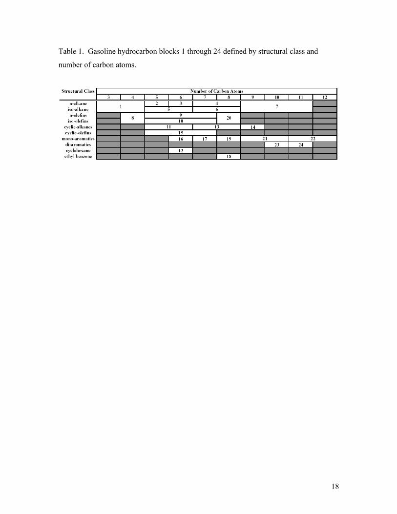
Table 1. Gasoline hydrocarbon blocks 1 through 24 defined by structural class and

number of carbon atoms.

18

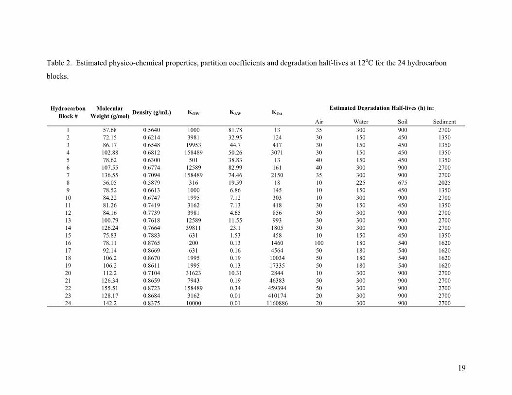
Table 2. Estimated physico-chemical properties, partition coefficients and degradation half-lives at 12oC for the 24 hydrocarbon

blocks.

Air Water Soil Sediment1 57.68 0.5640 1000 81.78 13 35 300 900 27002 72.15 0.6214 3981 32.95 124 30 150 450 13503 86.17 0.6548 19953 44.7 417 30 150 450 13504 102.88 0.6812 158489 50.26 3071 30 150 450 13505 78.62 0.6300 501 38.83 13 40 150 450 13506 107.55 0.6774 12589 82.99 161 40 300 900 27007 136.55 0.7094 158489 74.46 2150 35 300 900 27008 56.05 0.5879 316 19.59 18 10 225 675 20259 78.52 0.6613 1000 6.86 145 10 150 450 1350

10 84.22 0.6747 1995 7.12 303 10 300 900 270011 81.26 0.7419 3162 7.13 418 30 150 450 135012 84.16 0.7739 3981 4.65 856 30 300 900 270013 100.79 0.7618 12589 11.55 993 30 300 900 270014 126.24 0.7664 39811 23.1 1805 30 300 900 270015 75.83 0.7883 631 1.53 458 10 150 450 135016 78.11 0.8765 200 0.13 1460 100 180 540 162017 92.14 0.8669 631 0.16 4564 50 180 540 162018 106.2 0.8670 1995 0.19 10034 50 180 540 162019 106.2 0.8611 1995 0.13 17335 50 180 540 162020 112.2 0.7104 31623 10.31 2844 10 300 900 270021 126.34 0.8659 7943 0.19 46383 50 300 900 270022 155.51 0.8723 158489 0.34 459394 50 300 900 270023 128.17 0.8684 3162 0.01 410174 20 300 900 270024 142.2 0.8375 10000 0.01 1160886 20 300 900 2700

KAW KOAEstimated Degradation Half-lives (h) in:Hydrocarbon

Block #Molecular

Weight (g/mol) Density (g/mL) KOW

19

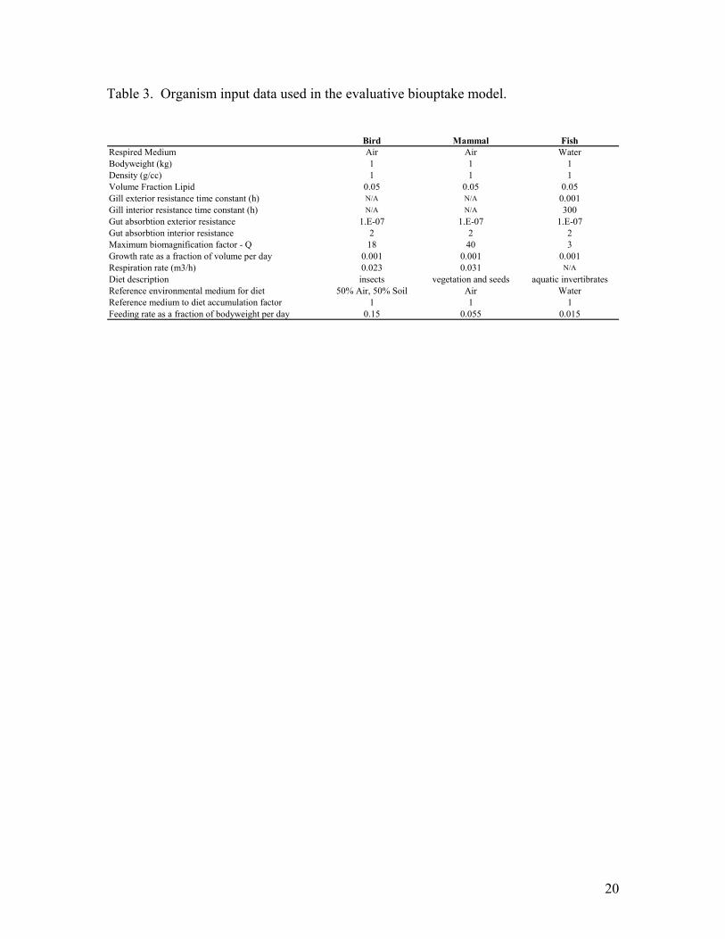
Table 3. Organism input data used in the evaluative biouptake model.

Bird Mammal Fish

Respired Medium Air Air WaterBodyweight (kg) 1 1 1Density (g/cc) 1 1 1Volume Fraction Lipid 0.05 0.05 0.05Gill exterior resistance time constant (h) N/A N/A 0.001Gill interior resistance time constant (h) N/A N/A 300Gut absorbtion exterior resistance 1.E-07 1.E-07 1.E-07Gut absorbtion interior resistance 2 2 2Maximum biomagnification factor - Q 18 40 3Growth rate as a fraction of volume per day 0.001 0.001 0.001Respiration rate (m3/h) 0.023 0.031 N/ADiet description insects vegetation and seeds aquatic invertibratesReference environmental medium for diet 50% Air, 50% Soil Air WaterReference medium to diet accumulation factor 1 1 1Feeding rate as a fraction of bodyweight per day 0.15 0.055 0.015

20

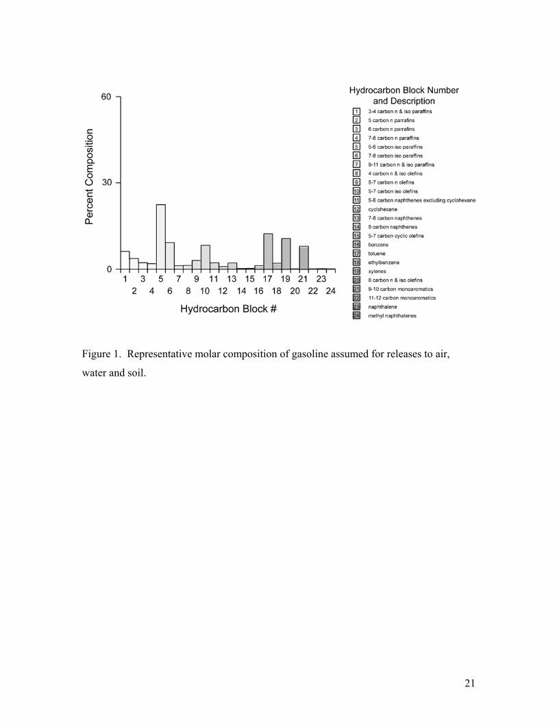
Figure 1. Representative molar composition of gasoline assumed for releases to air,

water and soil.

21

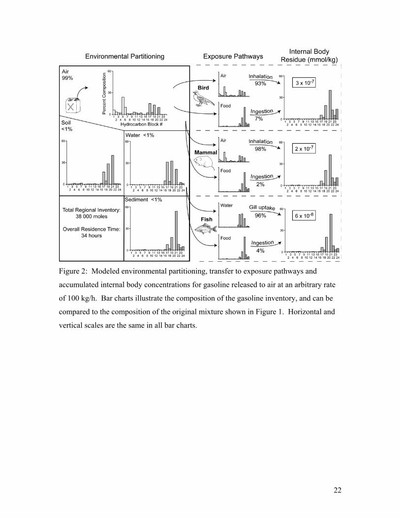
Figure 2: Modeled environmental partitioning, transfer to exposure pathways and

accumulated internal body concentrations for gasoline released to air at an arbitrary rate

of 100 kg/h. Bar charts illustrate the composition of the gasoline inventory, and can be

compared to the composition of the original mixture shown in Figure 1. Horizontal and

vertical scales are the same in all bar charts.

22

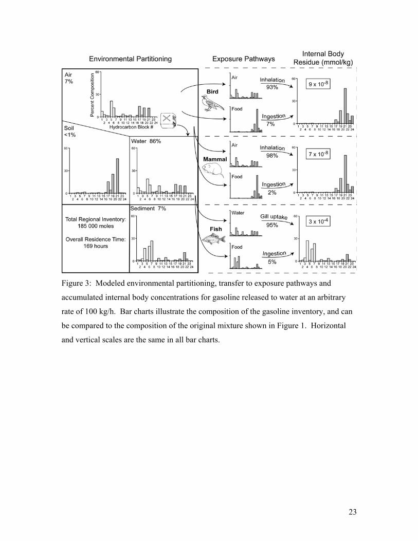
Figure 3: Modeled environmental partitioning, transfer to exposure pathways and

accumulated internal body concentrations for gasoline released to water at an arbitrary

rate of 100 kg/h. Bar charts illustrate the composition of the gasoline inventory, and can

be compared to the composition of the original mixture shown in Figure 1. Horizontal

and vertical scales are the same in all bar charts.

23

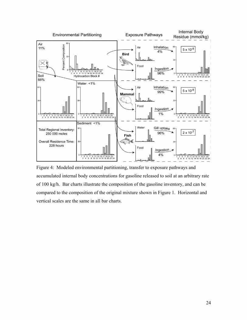
Figure 4: Modeled environmental partitioning, transfer to exposure pathways and

accumulated internal body concentrations for gasoline released to soil at an arbitrary rate

of 100 kg/h. Bar charts illustrate the composition of the gasoline inventory, and can be

compared to the composition of the original mixture shown in Figure 1. Horizontal and

vertical scales are the same in all bar charts.

24

References

(1) Posthuma, L.; Traas, T.R.; Suter, G.W. In: Species Sensitivity Distributions in

Ecotoxicology; Posthuma, L.; Suter, G.W.; Trass, T. P., Eds.; Lewis Publishers:

Boca Raton, 2002.

(2) Udo de Haes, H. A.; Finnveden, G.; Goedkoop, M.; Hauschild, M.; Hertwich, E.;

Hofstetter, P.; Jolliet, O.; Klöpffer, W.; Krewitt, W.; Lindeijer, E.; Mueller-Wenk,

R.; Olsen, I.; Pennington, D.; Potting, J.; Steen, B. Life-cycle impact assessment:

Striving towards best practice; Society of Environmental Toxicology and

Chemistry Press: Pensacola, FL, 2002.

(3) McDonough, W.; Braungart, M.; Anastas, P. T.; Zimmerman, J. B. Environmental

Science & Technology 2003, 37, 434A-441A.

(4) MacLeod, M.; McKone, T. E. Environmental Toxicology and Chemistry 2004, (in

press).

(5) Hill, R. A.; Chapman, P. M.; Mann, G. S.; Lawrence, G. S. Marine Pollution

Bulletin 2000, 40, 471-477.

(6) Suter, G. W.; Bartell, S. In Ecological risk assessment; Suter, G. W., Ed.; Lewis

Publishers: Boca Raton, FL, 1993, pp 275 -310.

(7) McCarty, L. S.; Mackay, D. Environmental Science & Technology 1993, 27,

1719-1728.

(8) Barron, M. G.; Hansen, J. A.; Lipton, J. Reviews Of Environmental

Contamination And Toxicology 2002, 173, 1-37.

(9) Escher, B. I.; Hermens, J. L. M. Environmental Science & Technology 2002, 36,

4201-4217.

(10) Jarvinen, A. W.; Ankley, G. T. Linkage of effects to tissue residues: Development

of a comprehensive database for aquatic organisms exposed to inorganic and

organic chemicals; Society of Environmental Toxicology and Chemistry Press:

Pensacola, FL, 1999.

(11) Mackay, D.; McCarty, L. S.; MacLeod, M. Environmental Toxicology &

Chemistry 2001, 20, 1491-1498.

25

(12) Dyer, S. D.; White-Hull, C. E.; Shephard, B. K. Environmental Science &

Technology 2000, 34, 2518-2524.

(13) USEPA (United States Environmental Protection Agency). Guidlines for

ecological risk assessment; United States Environmental Protection Agency

(http://www.erg.com/portfolio/elearn/ecorisk/html/resource/guidelines.pdf):

Washington, DC, 1998.

(14) DOE. Petroleum quick stats; United States Department of Energy Energy

Information Administration (http://www.eia.doe.gov/): Washington, DC, 2004.

(15) Foster, K.; Mackay, D.; Milford, L.; Webster, E. Multimedia modeling and

exposure assessment for gasoline; Trent University: Peterborough, ON, Canada,

2003.

(16) Mackay, D.; Diguardo, A.; Paterson, S.; Cowan, C. E. Environmental Toxicology

& Chemistry 1996, 15, 1627-1637.

(17) Peters, R. H. The ecological implications of body size; Cambridge University

Press: Cambridge, UK, 1983.

(18) Frappell, P. B.; Hinds, D. S.; Boggs, D. F. Physiological & Biochemical Zoology

2001, 74, 75-89.

(19) Mackay, D.; Fraser, A. Environmental Pollution 2000, 110, 375-391.

(20) Gobas, F. A. P. C.; Morrison, H. A. In Handbook of property estimation methods

for chemicals; Boethling, R. S., Mackay, D., Eds.; Lewis Publishers: Boca Raton,

2000.

(21) Gobas, F. Ecological Modelling 1993, 69, 1-17.

(22) Thomann, R. V. Environmental Science & Technology 1989, 18, 65-71.

(23) Paquin, P. R.; Farley, K.; Santore, R. C.; Kavvadas, C. D.; Mooney, K. G.;

Winfield, R. P.; Wu, K.-B.; DiToro, D. M. Metal in aquatic systems: A review of

exposure, bioaccumulation and toxicity models; Society of Environmental

Toxicology and Chemistry: Pensacola, FL, 2003.

(24) Kelly, B. C.; Gobas, F. Environmental Science & Technology 2003, 37, 2966-

2974.

(25) Mackay, D. Multimedia environmental models: The fugacity approach.; Lewis

Publishers: Boca Raton, Florida, 2001.

26

27

(26) Vanwezel, A. P.; Opperhuizen, A. Critical Reviews in Toxicology 1995, 25, 255-

279.

(27) DiToro, D.M.; McGrath, J.A.; Hansen, D.J. Environ. Toxicol. Chem 2000, 19,

1951-1970.

(28) Cahill, T. M.; Cousins, I.; MacKay, D. Environmental Toxicology and Chemistry

2003, 22, 26-34.

(29) USEPA (United States Environmental Protection Agency). Integrated risk

information system (IRIS); United States Environmental Protection Agency

(http://www.epa.gov/iris/): Washington, DC, 2004.

(30) Russom, C.; Bradbury, S.P.; Broderius, S.J. Env. Tox. Chem. 1997, 16, 5, 948-

967.

(31) Verhaar, H.J.M; Solbe, J.; Speksnijden, J.; van Leeuwen, C.J.; Hermens, J.L.M.

Chemosphere 2000, 40, 875-883.