Application of Total Least Squares to the Derivation of Closed-Form Green's Functions for Planar Layered Media

268 IEEE TRANSACTIONS ON MICROWAVE THEORY AND TECHNIQUES, VOL. 55, NO. 2, FEBRUARY 2007

Application of Total Least Squares to theDerivation of Closed-Form Green’sFunctions for Planar Layered Media

Rafael R. Boix, Member, IEEE, Francisco Mesa, Member, IEEE, and Francisco Medina, Senior Member, IEEE

Abstract—A new technique is presented for the numericalderivation of closed-form expressions of spatial-domain Green’sfunctions for multilayered media. In the new technique, thespectral-domain Green’s functions are approximated by anasymptotic term plus a ratio of two polynomials, the coefficientsof these two polynomials being determined via the method oftotal least squares. The approximation makes it possible to obtainclosed-form expressions of the spatial-domain Green’s functionsconsisting of a term containing the near-field singularities plusa finite sum of Hankel functions. A judicious choice of the coef-ficients of the spectral-domain polynomials prevents the Hankelfunctions from introducing nonphysical singularities as the hor-izontal separation between source and field points goes to zero.The new numerical technique requires very few computationalresources, and it has the merit of providing single closed-formapproximations for the Green’s functions that are accurate bothin the near and far fields. A very good agreement has been foundwhen comparing the results obtained with the new techniquewith those obtained via a numerically intensive computation ofSommerfeld integrals.

Index Terms—Green’s functions, layered media, Sommerfeld in-tegrals.

I. INTRODUCTION

THE application of the method of moments to the solutionof mixed-potential integral equations has proven to be a

powerful numerical tool in the analysis of planar circuits andantennas [1], [2], as well as in the study of the scattering prop-erties of objects that are partially/completely buried in earth [3],[4]. In fact, current commercial software products that are exten-sively used in the design of planar circuits and antennas (such asAnsoft’s Ensemble, Zeland’s IE3D, and Agilent’s Momentum)are based on a mixed-potential integral-equation approach. Onecrucial step in the application of the method of moments tomixed-potential integral equations is the numerical computationof spatial-domain Green’s functions for the scalar and vectorpotentials in multilayered media [5], [6]. These Green’s func-tions can be expressed as infinite integrals of spectral-domain

Manuscript received May 15, 2006; revised September 27, 2006. This workwas supported by the Spanish Ministerio de Educación y Ciencia and EuropeanUnion FEDER funds under Project TEC2004-03214 and by the Junta de An-dalucía under Project TIC-253.

R. R. Boix and F. Medina are with the Microwaves Group, Department ofElectronics and Electromagnetism, College of Physics, University of Seville,41012 Seville, Spain (e-mail: [email protected]).

F. Mesa is with the Microwaves Group, Department of Applied Physics 1, Es-cuela Técnica Superior de Ingeniería Informática, University of Seville, 41012Seville, Spain (e-mail: [email protected]).

Digital Object Identifier 10.1109/TMTT.2006.889336

Green’s functions that are commonly known as Sommerfeld in-tegrals. Owing to the slowly decaying and highly oscillating be-havior of the functions to be integrated, the brute-force numer-ical computation of Sommerfeld integrals is a time-consumingprocess. Therefore, in order to save CPU time in the solutionof mixed-potential integral equations, an extensive research hasbeen carried out over the last two decades to accelerate the com-putation of Sommerfeld integrals.

Some of the methods proposed for the fast computation ofSommerfeld integrals are based on tailor-made numerical inte-gration techniques. These techniques include the weighted-av-erage algorithm [5], [7] and related extrapolation algorithms [8],the integration along the imaginary axis of the spectral com-plex plane [7], [9], the integration along the steepest descentpath [10], and the integration with a window function as a con-volution kernel [11]. Although these techniques are all pow-erful numerical tools for the computation of Sommerfeld inte-grals, they have to be repeatedly used in the application of themethod of moments as the distance between source and fieldpoints changes, which limits their numerical efficiency. One al-ternative, which partially alleviates this problem, is to combinenumerical integration with the use of the fast Hankel transform[12]. A different approach to the computation of Sommerfeld in-tegrals is based on the application of asymptotic methods suchas the steepest descent method and the stationary phase method.These methods lead to asymptotic closed-form expressions ofGreen’s functions that are valid in a wide range of distances be-tween source and field points (typically above one wavelength)[10], [13], [14]. However, these expressions have been obtainedonly for simple layered media containing two or three differentmaterials, and extension of the methods to layered media withan arbitrary number of materials seems to be a difficult task.

One method that has reached a prominent position in thecomputation of Green’s functions for multilayered media is thediscrete complex image method [15]–[31]. In this method, thespectral-domain Green’s functions are approximated in termsof certain functions for which Sommerfeld integrals can be ob-tained in closed form. The method avoids numerical integrationand provides results that are valid in a wide range of distancesbetween source and field points. However, there is no commonagreement in the functions that should be used in the approxi-mation of the spectral-domain Green’s functions. For some re-searchers, the spectral-domain Green’s functions should be ex-clusively approximated in terms of complex exponentials thatare fitted by means of the generalized pencil of functions or ma-trix pencil method [18], [19], [25], [26], [28], [30], [31]. One

0018-9480/$25.00 © 2007 IEEE

BOIX et al.: APPLICATION OF TOTAL LEAST SQUARES TO DERIVATION OF CLOSED-FORM GREEN’S FUNCTIONS FOR PLANAR LAYERED MEDIA 269

drawback of this approach is that unpredictable large errors arisein the far-field computation of the spatial-domain Green’s func-tions [27], [30]–[32]. Recently, Yuan et al. [31] have found thatthe value of (horizontal separation between source and fieldpoints) marking the onset of far-field numerical errors can bemade much larger by increasing the number of complex expo-nentials used in the approximations, but it may lead to a consid-erable CPU time consumption (see [31, Table I]). In accordancewith the results shown in [27] and [29], the discrete compleximage method improves its stability when the complex expo-nentials used in the approximations of the spectral Green’s func-tions are accompanied by both a quasi-static term contributingthe near field and a surface-waves term accounting for the farfield. This is the approach originally proposed in [16] and fol-lowed in [17], [20]–[24], [27], and [29]. The drawback of thisapproach is that the surface-waves term contains poles of thespectral-domain Green’s functions, as well as residues of theGreen’s functions at these poles, and the accurate determina-tion of both the poles and the residues requires time-consumingalgorithms [24], [29]. It has also been stated that the Hankelfunctions of the surface-waves term introduce near-field singu-larities in the spatial-domain Green’s functions that do not existwhen source and field points are placed in different horizontalplanes of a multilayered media (i.e., when ) [20], [23],[24]. Fortunately, this latter problem can be solved by using theerror analysis technique proposed in [29].

A few years ago, Okhmatovski and Cangellaris introduceda new numerical method for the derivation of closed-form ex-pressions for multilayered media Green’s functions [32]. In theirproposal, the spectral-domain Green’s functions are representedin pole-residue form, and the poles and residues are numericallycomputed by means of a finite-difference approximation of theboundary value equations in the spectral domain. As a result ofthis, the spatial-domain Green’s functions are expressed as fi-nite series of Hankel functions representing cylindrical waves.The main drawback of this method is that the computational costbecomes very high in the near-field region since the number ofterms required for the accurate approximation of the Green’sfunctions grows very quickly as . More recently, Can-gellaris and his collaborators proposed an alternative formula-tion of the method where the poles and residues of the spec-tral-domain Green’s functions are computed by means of an it-erative algorithm called the vector-fitting algorithm [33], [34].Although this new approach makes it possible to reduce thenumber of Hankel functions used in the approximation of thespatial-domain Green’s functions, the vector-fitting algorithmis computationally demanding and does not suffice to eliminatethe near-field numerical problems of the original method, as rec-ognized in [34].

In this paper, a new numerical technique is presented for thederivation of closed-form Green’s functions both in the spec-tral and spatial domains. The technique borrows several ideasfrom [32]–[34], but it does not share the drawbacks of the ap-proaches followed in these papers. In the new technique, everyspectral-domain Green’s function is approximated in terms ofan asymptotic term plus a fraction of two polynomials. Theasymptotic terms are chosen in such a way that their spatial-do-main counterparts account for the singular or quasi-singular be-

havior of the spatial-domain Green’s functions as [34],[35]. Concerning the coefficients of the polynomials of the ap-proximation, they are computed via the method of total leastsquares following an approach similar to that reported in [36].Once an explicit expression for the fraction of polynomials isavailable, this expression is converted into a partial fraction ex-pansion (pole-residue form), which makes it possible to write itsspatial counterpart as a short series of Hankel functions. TheseHankel functions introduce nonexisting singularities as ,but these singularities are eliminated by suppressing some ofthe polynomials coefficients. As a result, our technique leads tosingle closed-form expressions of the spatial Green’s functionsthat are accurate both in the near and far fields (i.e., in the wholerange of values of ), as it happens with the expressions of [29].However, the CPU time required by the new technique is muchsmaller than that required in [29] for the following two mainreasons.

• Although a singular-value decomposition is carried out byboth the method of total least squares in the new tech-nique and the matrix pencil method in the discrete compleximage technique, the size of the matrix required by totalleast squares in the new technique is much smaller thanthat handled by the matrix pencil method in the discretecomplex image technique, which considerably reduces thenumber of operations.

• The new technique only requires to compute the poles andresidues of a fraction of polynomials, which is much sim-pler than computing the poles and residues of the spec-tral-domain Green’s functions of an arbitrary multilayeredmedia [29].

This paper is organized as follows. The derivation ofclosed-form expressions of multilayered media Green’s func-tions is presented in Section II, which also describes in detailthe strategies followed for eliminating nonexisting singulari-ties both in the spectral- and spatial-domain approximations.Section III provides numerical results for the spatial-domainGreen’s functions of scalar and vector potentials both in thenear and far fields. These results are compared with resultsobtained via numerical computation of Sommerfeld integrals,and good agreement is found in all cases. Conclusions aresummarized in Section IV.

II. THEORY

Let be the coordinates of an arbitrary field point ina multilayered substrate, and let be the coordinatesof an infinitesimal electric dipole source embedded in the mul-tilayered substrate (since the treatment of magnetic sources isanalogous to that of electric sources by virtue of the duality prin-ciple [6], only electric sources will be considered in this study).With respect to a reference frame centered at the source point,the radial and angular cylindrical coordinates of the field pointwill be (see [6, eq. (36)])

(1)

(2)

270 IEEE TRANSACTIONS ON MICROWAVE THEORY AND TECHNIQUES, VOL. 55, NO. 2, FEBRUARY 2007

Among the different mixed-potential integral-equation for-mulations [6], it will be the formulation C of Michalski andZheng [37] what will be used in this study. For the aforemen-tioned electric source in a multilayered substrate, let bea generic function representing either the corrected scalar po-tential Green’s function of [37] or any of the diagonal ele-ments of the corrected dyadic vector-potential Green’s function

of [37] ( is defined in terms of the traditional vector-po-tential Green’s function and the so-called correction factor

). In the frame of formulation C, the functionscan be written as Sommerfeld integrals of the type [37]

(3)

where is the spectral-domain counterpart of ,is the Bessel function of first kind and order zero, and

is an integration path in the first quadrant of the complex-plane that detours around the poles and branch points of

(see [8, Fig. 1]).Let be a generic function representing any of the

off-diagonal elements of . In formulation C, the functionscan be all expressed in terms of Sommerfeld integrals

of the type [37]

(4)

where is the spectral-domain counterpart of ,or are multiplying factors ( appears in

and , and appears in and ), and is theBessel function of first kind and order 1.

In [32], Okhmatovski and Cangellaris used a finite-differencescheme to prove that the spectral-domain functions and

can be approximately written as pole-residue finite se-ries of the form

(5)

When (5) is introduced in (3) and (4), closed-form expres-sions of and are obtained in terms of finite sumsof Hankel functions [32]. The problem with these finite sumsis that they require a very large value of for obtaining accu-rate values of and as [32]. In an attemptto overcome this problem, Kourkoulos and Cangellaris have re-cently suggested that the Hankel functions series should be com-bined with a closed-form quasi-static term accounting for thenear-field contributions to the Green’s functions [34]. Unfortu-nately, the introduction of this quasi-static term does not alwayssuffice to solve the near-field convergence problems reported in[32]. The origin of these numerical problems is that the Hankel

functions used in [32] and [34] introduce nonphysical singular-ities as , which is a well-known phenomenon [20], [23],[24], [29], [34]. If a quasi-static term is added to the Hankelfunctions, as in [34], the near-field problems are only eliminatedin the particular cases where the Green’s functions are singularas (e.g., shows this behavior when the source andfield points are in the same horizontal plane, i.e., when )since, in those cases, the quasi-static term is also singular, andthis singularity dominates over the Hankel functions singulari-ties [29]. However, when the Green’s functions are not singularas (e.g., when the source and field points are in differenthorizontal planes, i.e., when ), the quasi-static term is notsingular either and, therefore, it cannot mask the nonphysicalsingularities introduced by the Hankel functions.

In the following, a new approach is proposed for calculatingclosed-form spatial-domain Green’s functions. Our proposal issimilar to that of [34], but does not suffer from inaccuraciesrelated to Hankel functions singularities. In the new approach,the spectral-domain Green’s functions and arewritten as

(6)

where denotes the asymptotic behaviorsof for large values of . Note that, in (6),every spectral-domain Green’s function is approximated bymeans of the pole-residue representation of (5) plus one asymp-totic term. In accordance with the explanations of [38], theasymptotic terms and determine the behaviorof and in the vicinity of , respectively.If (6) is to provide an accurate closed-form representation ofthe spatial-domain Green’s functions, the asymptotic terms

have to satisfy the following conditions.• They must have closed-form inverse Hankel transforms,

i.e., the Sommerfeld integrals arising from the introductionof in (3) and (4) must have closed-formexpressions.

• Their spatial-domain counterpart should reproduce the sin-gular or quasi-singular behavior of and as

.• They should not have spectral-domain singularities dif-

ferent from those of and .The asymptotic expressions defined in [34] and [35] for the

spectral-domain Green’s functions of a source in a multilayeredsubstrate are good candidates for since theyfulfill the first two conditions (they have a closed-form inverseHankel transform and they account for spatial-domain near-fieldsingularities). However, they do not satisfy the third condition.In fact, the spectral asymptotic expressions proposed in [34]and [35] have “additional” singularities (either at orat , where is the free-space wavenumber and

and are the relative permittivity and permeability of thesource layer) that are not present in and . Thus,the direct use of the spectral asymptotic expressions of [34] and[35] in (6) would raise numerical inaccuracies. Demuynck et al.addressed a possible solution to the problem of singularities inthe spectral asymptotic expressions. Their solution consists of

BOIX et al.: APPLICATION OF TOTAL LEAST SQUARES TO DERIVATION OF CLOSED-FORM GREEN’S FUNCTIONS FOR PLANAR LAYERED MEDIA 271

multiplying these expressions by a factor that cancels out the“additional” singularities and, at the same time, keeps the sameasymptotic behavior for large [38]. In this paper, we haveapplied the cancellation technique of [38] to the asymptotic ex-pressions of [35], and the new resulting asymptotic expressionshave been adopted for playing the role ofin (6). These new asymptotic expressions are no longer singularand satisfy the aforementioned three conditions. In Appendix I,the expressions of are presented in theparticular case of the spectral-domain Green’s functions for asimple one-layer microstrip structure.

Once the asymptotic terms of (6) havebeen chosen, the coefficients and ( ;

) have to be obtained. In [32], these coefficients arecomputed by means of a quasi-analytical method resulting froma finite-difference scheme. However, Kourkoulos and Cangel-laris [34] employ an iterative numerical algorithm (the vector-fitting algorithm) based on pole relocation of complex startingpoles [39]. In this paper, the approach used for the computa-tion of and is also numerical, and it is based on themethod of total least squares. In order to apply this method, thepole-residue term of (6) must be written as a fraction of twopolynomials [36] as follows:

(7)

where and are polynomials in the vari-able of degrees and , respectively. These two poly-nomials can be written as

(8)

(9)

where and are unknown coefficients that are relatedto the coefficients and of (6). When (8) and (9) areintroduced in (7), and the resulting expression is multiplied by

, it is obtained after some rearrangements that

(10)

Each of the equations of (10) poses one problem of linear pa-rameter estimation with unknown parameters and , andfor each of these problems, there is a best solution in the totalleast squares sense. In order to obtain that solution, the approx-imate expression of (10) is enforced to be exactly satisfied at

different values of the complex variable ,, which yields an overdetermined system

of linear equations. As explained in [40], this linear system of

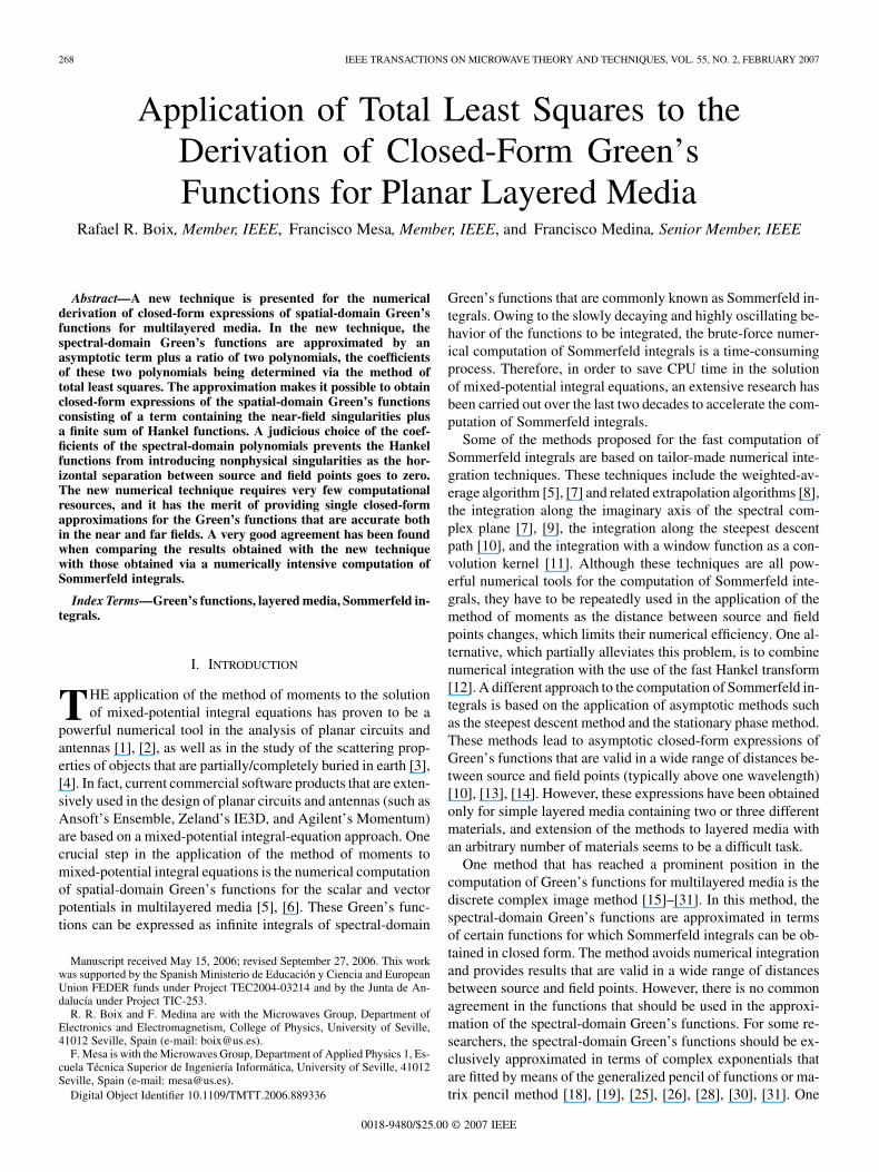
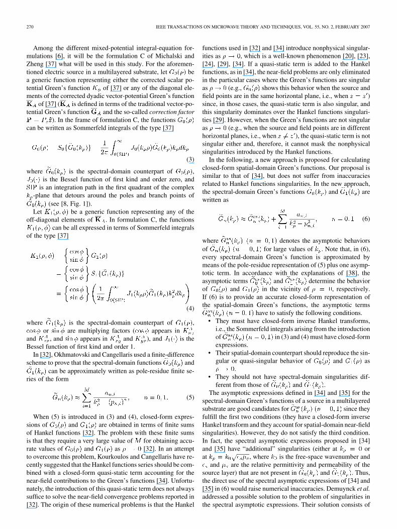
Fig. 1. Path chosen in the complex k =k -plane when applying the method oftotal least squares to (10).

equations can be solved via a singular-value decomposition forobtaining the minimum total least squares solution. Since thespectral-domain Green’s functions of lossless multilayered sub-strates have surface-wave singularities and branch-point singu-larities along the real axis of the complex -plane [5], in theapplication of the method of total least squares, it is convenientto sample (10) along a path in the complex -plane that detoursaround the singularities [16]. In this study, we have chosen apath, i.e., , that satisfies this last condition and that asymptot-ically approaches the real axis of the -plane; specifically

(11)

where determines the maximum imaginary value taken by thepath. The path defined by (11) is shown in Fig. 1. In our expe-rience, a good choice is to take andin (11), where is the maximum wavenumber among thelayers of the multilayered substrate. Anyway, numerical simu-lations have proven that the results obtained via the method oftotal least squares (see Section III) are not appreciably sensitiveto slight variations in the aforementioned values of and .

Once a total least squares solution has been obtained for thecoefficients and of (10), the coefficients of (6) (i.e.,the squared poles of the pole-residue term) can be determined asthe complex roots of the polynomial . These roots canbe readily extracted from the polynomial coefficients by com-puting the eigenvalues of the companion matrix, as explained in[41]. The coefficients can also be obtained in terms ofby using the standard residue definition

(12)

Regarding the computation of the coefficients and of(6), the application of the method of total least squares has twoadvantages over the vector-fitting algorithm [34]. First, whereasthe method of total least squares generates the poles and residuesin one step, the vector-fitting algorithm carries out an iterativesearch, the computation time required by each iteration beingcomparable to that required by the method of total least squaresas a whole. The second advantage is that the method of totalleast squares gives an estimate for (the number of terms re-tained in the pole-residue series) from the number of nonzero

272 IEEE TRANSACTIONS ON MICROWAVE THEORY AND TECHNIQUES, VOL. 55, NO. 2, FEBRUARY 2007

singular values obtained in the singular-value decomposition[36]. In Section III, it will be shown that values of lower than13 have always been found sufficient to obtain accurate approxi-mations of . These values of are certainlysmaller than those handled in [33] and [34], and considerablysmaller than those reported in [32].

When the approximation proposed in (6) is introduced in (3)and (4), and the Sommerfeld integrals are calculated [42], thefollowing expressions are obtained:

(13)

(14)

where are Hankel functions of the secondkind and order , and and can be written inclosed form in terms of functions of the type shown in (45) and(47). As mentioned above, the complex roots of the polynomial

provide the numerical values of ( ;

). Since the complex numbers and

( ; ) are all poles of [see (6)], thesign of the poles used in (13) and (14) has to be chosen insuch a way that , which ensures that thesolution obtained for and fulfills the causalityand radiation conditions [34].

As commented above, the functions and of(13) and (14) reproduce the behavior of and as

. In fact, and may have singularities as, and these singularities coincide with those of

and (as stated above, the singularities may be presentwhen the source and field points are in the same horizontal plane

, but they never appear when the source and field pointsare in different horizontal planes ). The Hankel functions

and of (13) and (14) also have singu-larities as , but these singularities are not shared byand , and this may have a detrimental effect on the accu-racy of (13) and (14) as [20], [23], [24]. In the remainderof this section, it will be shown that the coefficients canbe chosen in such a way that the sums of Hankel functions of(13) and (14) have a nonsingular smooth behavior in the vicinityof . In that case, the series of Hankel functions will notmask the correct behavior of and as , whichis provided by and .

In order to show the problem of Hankel functions singularitiesin the case of (13), the following expansion of as

[43] is used:

(15)

where is Euler’s constant [43]. If (15) is introduced in (13),the following expansion of as is obtained:

(16)

Equation (16) shows that the Hankel functions of (13) introducea logarithmic singularity as . However, note that this log-arithmic singularity can be suppressed if is en-forced. Looking at (6) and (7), the sum can be re-lated to the coefficients of the polynomial in thefollowing way:

(17)

Therefore, if is enforced, the coefficientof must be set to zero. According to this result,in order to avoid the effect of Hankel functions singularities as

in (13), a polynomial in of degree should beused in the numerator of the approximation (7) of . Thus,it is convenient to approximate as

(18)

where

(19)

The procedure designed for avoiding the effect of Hankel func-tions singularities in (13) can also be applied to (14). In thislatter case, the analysis of the singularities suggests to use thefollowing expansion of the functions as[43]:

(20)

BOIX et al.: APPLICATION OF TOTAL LEAST SQUARES TO DERIVATION OF CLOSED-FORM GREEN’S FUNCTIONS FOR PLANAR LAYERED MEDIA 273

Equation (20) must then be introduced in (14) in order to obtainthe expansion of as

(21)

Equation (21) shows that the Hankel functions of (14) introducea singularity of the type as . This singularity canbe eliminated provided that is enforced. How-ever, this condition does not always suffice to ensure that theHankel functions of (14) do not mask the behavior ofas . In fact, since as and(see [21, eq. (24)]) andas and , may tend tozero faster than as . If

has to go to zero faster than(or at least with the same decay rate), it is then necessary thatnot only in (21), but also .The two finite sums and can berelated to the coefficients of the polynomial inthe following way:

(22)

(23)

Therefore, if and are bothenforced, the coefficients and ofmust be set to zero. In conclusion, in order to avoid the effectof Hankel functions singularities in the approximation (14) of

as , the polynomial of the numerator in theapproximation (7) of has to be a polynomial in of

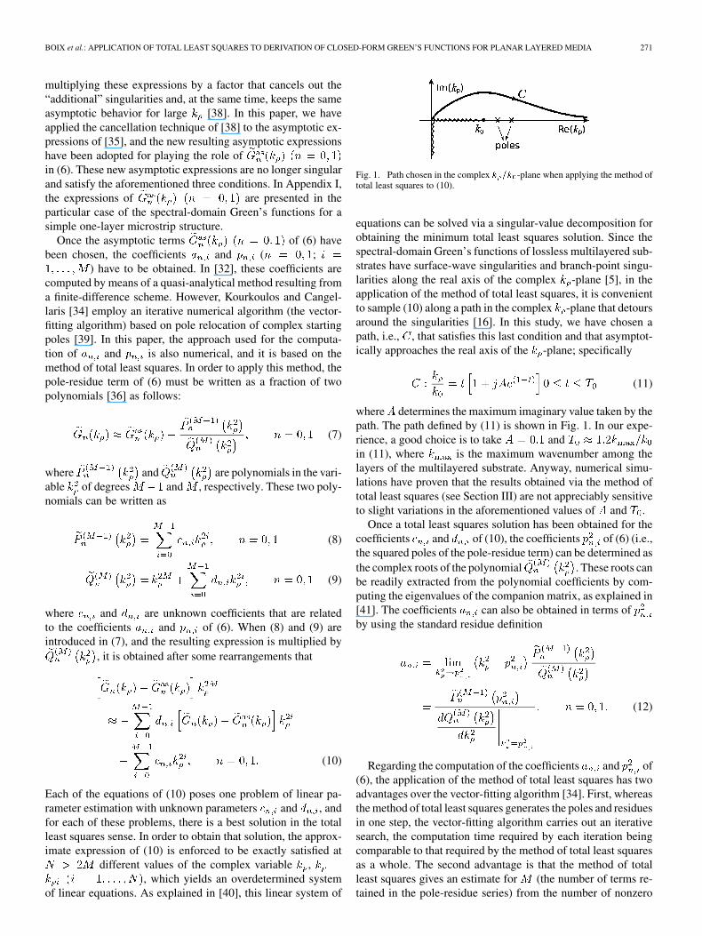
Fig. 2. One-layer substrate microstrip structure studied in this paper. Thesource point is in the air.

degree . Thus, the approximation of should bewritten as

(24)

where

(25)

It should be noted that the pole-residue terms of (6) and (7) wereoriginally proposed to decay at a rate for large . How-ever, in order to avoid problems in the approximation of the spa-tial-domain Green’s functions as , it has now been proventhat the pole-residue term of should decay at a ratefor large , and the pole-residue term of at a rate .This conclusion can be connected with the error analysis car-ried out in [29] where it was shown that singularity problemsencountered for in the application of the discrete com-plex image method can be solved when the surface-wave term of

decays at a rate for large , and the surface-waveterm of decays at a rate . Whereas the former resultis coherent with that obtained in this paper, there is a discrep-ancy in the latter result. In our opinion, the decay rate imposedin [29] to the surface-wave term of may be stricter thannecessary. In fact, if that surface-wave term is enforced to decayat a rate , this may probably suffice to eliminate the singu-larity problems discussed in [29].

III. NUMERICAL RESULTS

For demonstrative purposes, the method of Section II hasbeen applied to the computation of the Green’s functions of thesimple microstrip structure of Fig. 2 when the value of the rela-tive permittivity is and the value of the substrate thick-ness is mm. The results are presented in Figs. 3–11.

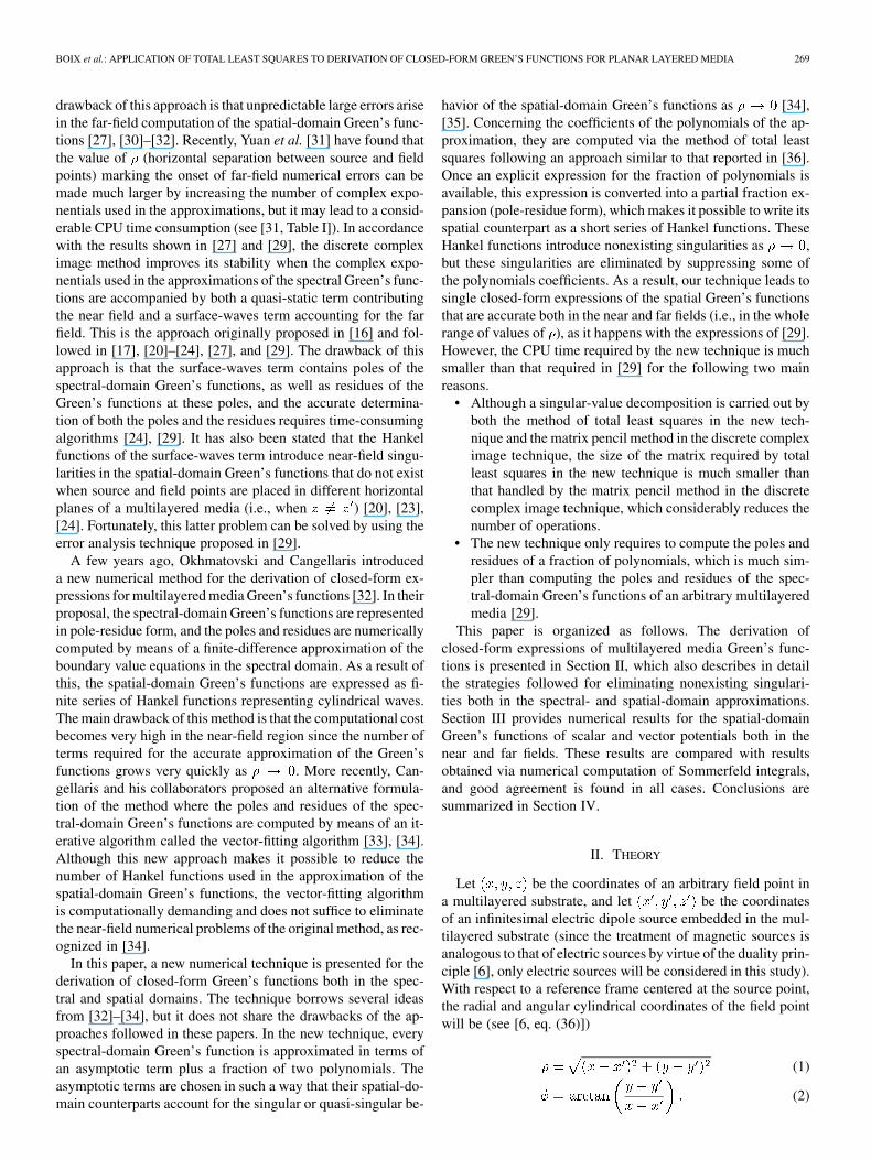
Fig. 3 shows results for the spectral-domain scalar potentialGreen’s function along the path of Fig. 1. An excellent agree-ment is found when the exact values of the spectral-domainGreen’s function are compared with the values arising from theapplication of the method of total least squares (18) (in all thefigures in this section, the results obtained via the method of totalleast squares will be denoted as TLS). The differences betweenthe two sets of results are always found to be below 0.03%.Since the approximation provided by the spectral-domain ex-pression (18) is very accurate, the approximation provided byits spatial-domain counterpart (13) should also be very accu-rate. This is verified in Fig. 4 where the results obtained with theclosed-form expression (13) are compared with results obtainedvia numerical integration of Sommerfeld integrals. Again, the

274 IEEE TRANSACTIONS ON MICROWAVE THEORY AND TECHNIQUES, VOL. 55, NO. 2, FEBRUARY 2007

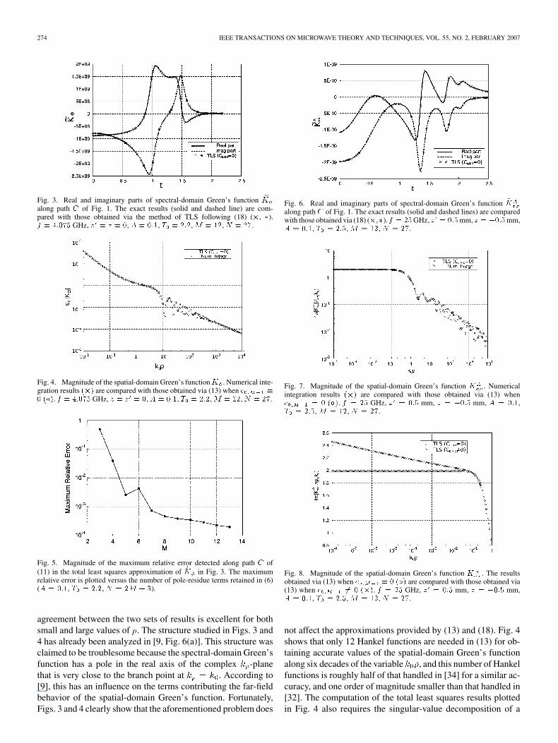
Fig. 3. Real and imaginary parts of spectral-domain Green’s function Kalong path C of Fig. 1. The exact results (solid and dashed line) are com-pared with those obtained via the method of TLS following (18) (�, �).f = 4:075 GHz, z = z = 0, A = 0:1, T = 2:2,M = 12,N = 27.

Fig. 4. Magnitude of the spatial-domain Green’s functionK . Numerical inte-gration results (�) are compared with those obtained via (13) when c =0 (�). f = 4:075GHz, z = z = 0, A = 0:1, T = 2:2,M = 12,N = 27.

Fig. 5. Magnitude of the maximum relative error detected along path C of(11) in the total least squares approximation of K in Fig. 3. The maximumrelative error is plotted versus the number of pole-residue terms retained in (6)(A = 0:1, T = 2:2, N = 2M + 3).

agreement between the two sets of results is excellent for bothsmall and large values of . The structure studied in Figs. 3 and4 has already been analyzed in [9, Fig. 6(a)]. This structure wasclaimed to be troublesome because the spectral-domain Green’sfunction has a pole in the real axis of the complex -planethat is very close to the branch point at . According to[9], this has an influence on the terms contributing the far-fieldbehavior of the spatial-domain Green’s function. Fortunately,Figs. 3 and 4 clearly show that the aforementioned problem does

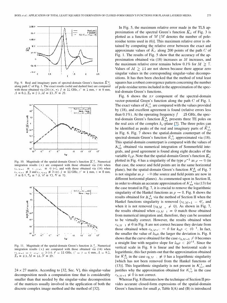
Fig. 6. Real and imaginary parts of spectral-domain Green’s function Kalong path C of Fig. 1. The exact results (solid and dashed lines) are comparedwith those obtained via (18) (�,�). f = 25GHz, z = 0:5mm, z = �0:5mm,A = 0:1, T = 2:5, M = 12, N = 27.

Fig. 7. Magnitude of the spatial-domain Green’s function K . Numericalintegration results (�) are compared with those obtained via (13) whenc = 0 (�). f = 25 GHz, z = 0:5 mm, z = �0:5 mm, A = 0:1,T = 2:5, M = 12, N = 27.

Fig. 8. Magnitude of the spatial-domain Green’s function K . The resultsobtained via (13) when c = 0 (�) are compared with those obtained via(13) when c 6= 0 (�). f = 25 GHz, z = 0:5 mm, z = �0:5 mm,A = 0:1, T = 2:5, M = 12, N = 27.

not affect the approximations provided by (13) and (18). Fig. 4shows that only 12 Hankel functions are needed in (13) for ob-taining accurate values of the spatial-domain Green’s functionalong six decades of the variable , and this number of Hankelfunctions is roughly half of that handled in [34] for a similar ac-curacy, and one order of magnitude smaller than that handled in[32]. The computation of the total least squares results plottedin Fig. 4 also requires the singular-value decomposition of a

BOIX et al.: APPLICATION OF TOTAL LEAST SQUARES TO DERIVATION OF CLOSED-FORM GREEN’S FUNCTIONS FOR PLANAR LAYERED MEDIA 275

Fig. 9. Real and imaginary parts of spectral-domain Green’s function Kalong path C of Fig. 1. The exact results (solid and dashed line) are comparedwith those obtained via (24) (�, �). f = 11 GHz, z = 1 mm, z = 0 mm,A = 0:1, T = 2:3, M = 13, N = 29.

Fig. 10. Magnitude of the spatial-domain Green’s function K . Numericalintegration results (�) are compared with those obtained via (14) whenc = c = 0 (�), and with those obtained via (14) whenc 6= 0 and c 6= 0 (�). f = 11 GHz, z = 1 mm, z = 0 mm,A = 0:1, T = 2:3, M = 13, N = 29.

Fig. 11. Magnitude of the spatial-domain Green’s function K . Numericalintegration results (�) are compared with those obtained via (14) whenc = c = 0 (�). f = 11 GHz, z = z = 0 mm, A = 0:1,T = 2:3, M = 13, N = 29.

24 27 matrix. According to [32, Sec. V], this singular-valuedecomposition needs a computation time that is considerablysmaller than that needed by the singular-value decompositionof the matrices usually involved in the application of both thediscrete complex image method and the method of [32].

In Fig. 5, the maximum relative error made in the TLS ap-proximation of the spectral Green’s function of Fig. 3 isplotted as a function of [ denotes the number of pole-residue terms used in (6)]. This maximum relative error is ob-tained by computing the relative error between the exact andapproximate values of along 200 points of the path ofFig. 1. The results of Fig. 5 show that the accuracy of the ap-proximation obtained via (18) increases as increases, andthe maximum relative error remains below 0.1% for .Values of are not shown because there appear zerosingular values in the corresponding singular-value decompo-sitions. It has then been checked that the method of total leastsquares has a robust convergence pattern concerning the numberof pole-residue terms included in the approximation of the spec-tral-domain Green’s functions.

Fig. 6 shows the component of the spectral-domainvector-potential Green’s function along the path of Fig. 1.The exact values of are compared with the values providedby (18), and excellent agreement is found (relative errors lessthan 0.1%). At the operating frequency GHz, the spec-tral-domain Green’s function presents three TE poles onthe real axis of the complex -plane [7]. The three poles canbe identified as peaks of the real and imaginary parts ofin Fig. 6. Fig. 7 shows the spatial-domain counterpart of thespectral-domain Green’s function approximated via (18).This spatial-domain counterpart is compared with the values of

obtained via numerical integration of Sommerfeld inte-grals, and good agreement is found along eight decades of thevariable . Note that the spatial-domain Green’s functionplotted in Fig. 4 has a singularity of the type as (inthat case, the source and field points are in the same horizontalplane), but the spatial-domain Green’s function of Fig. 7is not singular as (the source and field points are now indifferent horizontal planes). As commented upon in Section II,in order to obtain an accurate approximation of via (13) forthe case treated in Fig. 7, it is crucial to remove the logarithmicsingularity of the Hankel functions as . Fig. 8 shows theresults obtained for via the method of Section II when theHankel functions singularity is removed , andwhen it is not removed . As shown in Fig. 7,the results obtained when match those obtainedfrom numerical integration and, therefore, they can be assumedto be virtually correct. However, the results obtained when

in Fig. 8 are not correct because they deviate fromthose obtained when for . In fact,the smaller the value of , the larger the deviation is. Fig. 8shows that the curve obtained for the case becomesa straight line with negative slope for . Since thevertical scale in Fig. 8 is linear and the horizontal scale islogarithmic, this fact points out that the approximation obtainedfor in the case has a logarithmic singularity[which has not been removed from the Hankel functions of(13)]. This logarithmic singularity is not present in , andjustifies why the approximation obtained for in the case

is not correct.Whereas Fig. 8 illustrates how the technique of Section II pro-

vides accurate closed-form expressions of the spatial-domainGreen’s functions for small , Table I(A) and (B) is introduced

276 IEEE TRANSACTIONS ON MICROWAVE THEORY AND TECHNIQUES, VOL. 55, NO. 2, FEBRUARY 2007

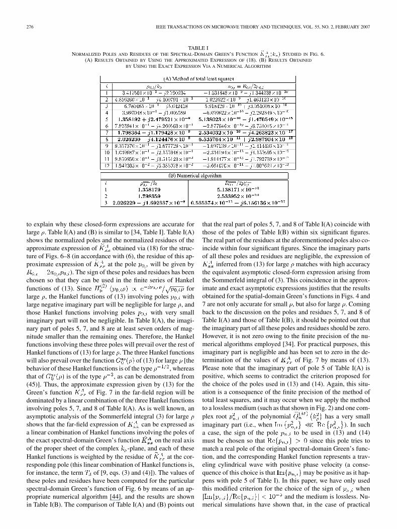
TABLE INORMALIZED POLES AND RESIDUES OF THE SPECTRAL-DOMAIN GREEN’S FUNCTION K (k ) STUDIED IN FIG. 6.

(A) RESULTS OBTAINED BY USING THE APPROXIMATED EXPRESSION OF (18). (B) RESULTS OBTAINED

BY USING THE EXACT EXPRESSION VIA A NUMERICAL ALGORITHM

to explain why these closed-form expressions are accurate forlarge . Table I(A) and (B) is similar to [34, Table I]. Table I(A)shows the normalized poles and the normalized residues of theapproximate expression of obtained via (18) for the struc-ture of Figs. 6–8 (in accordance with (6), the residue of this ap-proximate expression of at the pole will be given by

). The sign of these poles and residues has beenchosen so that they can be used in the finite series of Hankelfunctions of (13). Since forlarge , the Hankel functions of (13) involving poles withlarge negative imaginary part will be negligible for large , andthose Hankel functions involving poles with very smallimaginary part will not be negligible. In Table I(A), the imagi-nary part of poles 5, 7, and 8 are at least seven orders of mag-nitude smaller than the remaining ones. Therefore, the Hankelfunctions involving these three poles will prevail over the rest ofHankel functions of (13) for large . The three Hankel functionswill also prevail over the function of (13) for large [thebehavior of these Hankel functions is of the type , whereasthat of is of the type , as can be demonstrated from(45)]. Thus, the approximate expression given by (13) for theGreen’s function of Fig. 7 in the far-field region will bedominated by a linear combination of the three Hankel functionsinvolving poles 5, 7, and 8 of Table I(A). As is well known, anasymptotic analysis of the Sommerfeld integral (3) for largeshows that the far-field expression of can be expressed asa linear combination of Hankel functions involving the poles ofthe exact spectral-domain Green’s function on the real axisof the proper sheet of the complex -plane, and each of theseHankel functions is weighted by the residue of at the cor-responding pole (this linear combination of Hankel functions is,for instance, the term of [9, eqs. (3) and (4)]). The values ofthese poles and residues have been computed for the particularspectral-domain Green’s function of Fig. 6 by means of an ap-propriate numerical algorithm [44], and the results are shownin Table I(B). The comparison of Table I(A) and (B) points out

that the real part of poles 5, 7, and 8 of Table I(A) coincide withthose of the poles of Table I(B) within six significant figures.The real part of the residues at the aforementioned poles also co-incide within four significant figures. Since the imaginary partsof all these poles and residues are negligible, the expression of

inferred from (13) for large matches with high accuracythe equivalent asymptotic closed-form expression arising fromthe Sommerfeld integral of (3). This coincidence in the approx-imate and exact asymptotic expressions justifies that the resultsobtained for the spatial-domain Green’s functions in Figs. 4 and7 are not only accurate for small , but also for large . Comingback to the discussion on the poles and residues 5, 7, and 8 ofTable I(A) and those of Table I(B), it should be pointed out thatthe imaginary part of all these poles and residues should be zero.However, it is not zero owing to the finite precision of the nu-merical algorithms employed [34]. For practical purposes, thisimaginary part is negligible and has been set to zero in the de-termination of the values of of Fig. 7 by means of (13).Please note that the imaginary part of pole 5 of Table I(A) ispositive, which seems to contradict the criterion proposed forthe choice of the poles used in (13) and (14). Again, this situ-ation is a consequence of the finite precision of the method oftotal least squares, and it may occur when we apply the methodto a lossless medium (such as that shown in Fig. 2) and one com-plex root of the polynomial has a very smallimaginary part (i.e., when ). In sucha case, the sign of the pole to be used in (13) and (14)must be chosen so that since this pole tries tomatch a real pole of the original spectral-domain Green’s func-tion, and the corresponding Hankel function represents a trav-eling cylindrical wave with positive phase velocity (a conse-quence of this choice is that may be positive as it hap-pens with pole 5 of Table I). In this paper, we have only usedthis modified criterion for the choice of the sign of when

and the medium is lossless. Nu-merical simulations have shown that, in the case of practical

BOIX et al.: APPLICATION OF TOTAL LEAST SQUARES TO DERIVATION OF CLOSED-FORM GREEN’S FUNCTIONS FOR PLANAR LAYERED MEDIA 277

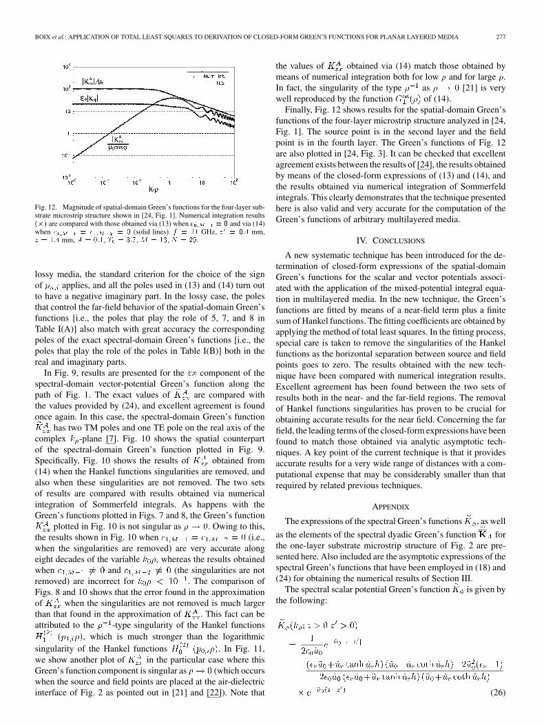
Fig. 12. Magnitude of spatial-domain Green’s functions for the four-layer sub-strate microstrip structure shown in [24, Fig. 1]. Numerical integration results(�) are compared with those obtained via (13) when c = 0 and via (14)when c = c = 0 (solid lines). f = 11 GHz, z = 0:4 mm,z = 1:4 mm, A = 0:1, T = 3:7, M = 13, N = 29.

lossy media, the standard criterion for the choice of the signof applies, and all the poles used in (13) and (14) turn outto have a negative imaginary part. In the lossy case, the polesthat control the far-field behavior of the spatial-domain Green’sfunctions [i.e., the poles that play the role of 5, 7, and 8 inTable I(A)] also match with great accuracy the correspondingpoles of the exact spectral-domain Green’s functions [i.e., thepoles that play the role of the poles in Table I(B)] both in thereal and imaginary parts.

In Fig. 9, results are presented for the component of thespectral-domain vector-potential Green’s function along thepath of Fig. 1. The exact values of are compared withthe values provided by (24), and excellent agreement is foundonce again. In this case, the spectral-domain Green’s function

has two TM poles and one TE pole on the real axis of thecomplex -plane [7]. Fig. 10 shows the spatial counterpartof the spectral-domain Green’s function plotted in Fig. 9.Specifically, Fig. 10 shows the results of obtained from(14) when the Hankel functions singularities are removed, andalso when these singularities are not removed. The two setsof results are compared with results obtained via numericalintegration of Sommerfeld integrals. As happens with theGreen’s functions plotted in Figs. 7 and 8, the Green’s function

plotted in Fig. 10 is not singular as . Owing to this,the results shown in Fig. 10 when (i.e.,when the singularities are removed) are very accurate alongeight decades of the variable , whereas the results obtainedwhen and (the singularities are notremoved) are incorrect for . The comparison ofFigs. 8 and 10 shows that the error found in the approximationof when the singularities are not removed is much largerthan that found in the approximation of . This fact can beattributed to the -type singularity of the Hankel functions

, which is much stronger than the logarithmicsingularity of the Hankel functions . In Fig. 11,we show another plot of in the particular case where thisGreen’s function component is singular as (which occurswhen the source and field points are placed at the air-dielectricinterface of Fig. 2 as pointed out in [21] and [22]). Note that

the values of obtained via (14) match those obtained bymeans of numerical integration both for low and for large .In fact, the singularity of the type as [21] is verywell reproduced by the function of (14).

Finally, Fig. 12 shows results for the spatial-domain Green’sfunctions of the four-layer microstrip structure analyzed in [24,Fig. 1]. The source point is in the second layer and the fieldpoint is in the fourth layer. The Green’s functions of Fig. 12are also plotted in [24, Fig. 3]. It can be checked that excellentagreement exists between the results of [24], the results obtainedby means of the closed-form expressions of (13) and (14), andthe results obtained via numerical integration of Sommerfeldintegrals. This clearly demonstrates that the technique presentedhere is also valid and very accurate for the computation of theGreen’s functions of arbitrary multilayered media.

IV. CONCLUSIONS

A new systematic technique has been introduced for the de-termination of closed-form expressions of the spatial-domainGreen’s functions for the scalar and vector potentials associ-ated with the application of the mixed-potential integral equa-tion in multilayered media. In the new technique, the Green’sfunctions are fitted by means of a near-field term plus a finitesum of Hankel functions. The fitting coefficients are obtained byapplying the method of total least squares. In the fitting process,special care is taken to remove the singularities of the Hankelfunctions as the horizontal separation between source and fieldpoints goes to zero. The results obtained with the new tech-nique have been compared with numerical integration results.Excellent agreement has been found between the two sets ofresults both in the near- and the far-field regions. The removalof Hankel functions singularities has proven to be crucial forobtaining accurate results for the near field. Concerning the farfield, the leading terms of the closed-form expressions have beenfound to match those obtained via analytic asymptotic tech-niques. A key point of the current technique is that it providesaccurate results for a very wide range of distances with a com-putational expense that may be considerably smaller than thatrequired by related previous techniques.

APPENDIX

The expressions of the spectral Green’s functions , as well

as the elements of the spectral dyadic Green’s function forthe one-layer substrate microstrip structure of Fig. 2 are pre-sented here. Also included are the asymptotic expressions of thespectral Green’s functions that have been employed in (18) and(24) for obtaining the numerical results of Section III.

The spectral scalar potential Green’s function is given bythe following:

(26)

278 IEEE TRANSACTIONS ON MICROWAVE THEORY AND TECHNIQUES, VOL. 55, NO. 2, FEBRUARY 2007

(27)

where and . The asymptotic

expressions of can then be written as

(28)

(29)

where (in an arbitrary multilayered mediumshould be taken as , with being the max-

imum wavenumber among the layers of the medium [38]). Notethat the factor has been deliberately introduced in(28) and (29) in order to avoid the singularity of the function

when [38]. Since the function is not singularwhen , the function should not be singular either

[remember that is involved in the approximation of , asshown in (6)].

The diagonal elements of are and [37]. Theexpressions of can be written as

(30)

(31)

and the asymptotic expressions of are given by

(32)

(33)

The expressions of are

(34)

(35)

and the asymptotic expressions of are

(36)

(37)

The off-diagonal elements of are , , , and[37]. The expressions of and are

(38)

(39)

where and are the Cartesian spectral variables associ-ated with and , respectively (and related to via

). The asymptotic expressions of and are

(40)

(41)

BOIX et al.: APPLICATION OF TOTAL LEAST SQUARES TO DERIVATION OF CLOSED-FORM GREEN’S FUNCTIONS FOR PLANAR LAYERED MEDIA 279

Once again, the factor has been introduced in (40)and (41) to avoid that and are singular when

[38]. Finally, and are relatedto and by means of

(42)

(43)

and, as a consequence of these relations, and.

Looking at (28), (29), (32), (33), (36), and (37), it can be ob-served that the functions denoted in this paper by (i.e.,

, and ) are all linear combinations of functionsof the type

(44)

where . It means that the functions of (13) willall be linear combinations of functions of the type [42]

(45)

If , the functions show a singularity of the typeas . In accordance with (28), (29), (32), (33), (36), and(37), this means that, in the case , the functionswill show the same singularity as . According to (3) and(13), the singularity will also be present in , which is inagreement with the near-field behavior of described in[20].

According to (40) and (41), the functions denotedin this paper by (i.e., and

) are functions of the type

(46)

where . Therefore, the functions of (14) will be

functions of the type [42]

(47)

It can be shown that as and , butas and . Looking at (40) and (41),

this means that in the case (i.e., the source andfield and points are placed at the interface between the air andthe dielectric layer in Fig. 2), the functions will showa singularity of the type as . According to (4) and(14), this singularity will be reproduced in , which is inagreement with the behavior of predicted in [21].

REFERENCES

[1] J. R. Mosig, “Arbitrarily shaped microstrip structures and their analysiswith a mixed potential integral equation,” IEEE Trans. Microw. TheoryTech., vol. 36, no. 2, pp. 314–323, Feb. 1988.

[2] R. C. Hall and J. R. Mosig, “The analysis of arbitrarily shaped aperture-coupled patch antennas via a mixed-potential integral equation,” IEEETrans. Antennas Propag., vol. 44, no. 5, pp. 608–614, May 1996.

[3] K. A. Michalski and D. Zheng, “Electromagnetic scattering and ra-diation by surfaces of arbitrary shape in layered media—Part II: Im-plementation and results for contiguous half-spaces,” IEEE Trans. An-tennas Propag., vol. 38, no. 3, pp. 345–352, Mar. 1990.

[4] S. Vitebskiy, K. Sturgess, and L. Carin, “Short-pulse plane-wave scat-tering from buried perfectly conducting bodies of revolution,” IEEETrans. Antennas Propag., vol. 44, no. 2, pp. 143–151, Feb. 1996.

[5] J. R. Mosig, “Integral equation technique,” in Numerical Techniquesfor Microwave and Millimeter-Wave Passive Structures, T. Itoh, Ed.New York: Wiley, 1989, pp. 133–213.

[6] K. A. Michalski and J. R. Mosig, “Multilayered media Green’sfunctions in integral equation formulations,” IEEE Trans. AntennasPropag., vol. 45, no. 3, pp. 508–519, Mar. 1997.

[7] J. R. Mosig and F. E. Gardiol, “Analytical and numerical techniques inthe Green’s function treatment of microstrip antennas and scatterers,”Proc. Inst. Elect. Eng., vol. 130, no. 2, pt. H, pp. 175–182, Mar. 1983.

[8] K. A. Michalski, “Extrapolation methods for Sommerfeld integraltails,” IEEE Trans. Antennas Propag., vol. 46, no. 10, pp. 1405–1418,Oct. 1998.

[9] J. R. Mosig and Álvarez-Melcón, “Green’s functions in lossy layeredmedia: Integration along the imaginary axis and asymptotic behavior,”IEEE Trans. Antennas Propag., vol. 51, no. 12, pp. 3200–3208, Dec.2003.

[10] T. J. Cui and W. C. Chew, “Fast evaluation of Sommerfeld integralsfor EM scattering and radiation by three-dimensional buried objects,”IEEE Trans. Geosci. Remote Sens., vol. 37, no. 3, pp. 887–900, Mar.1999.

[11] W. Cai and T. Yu, “Fast calculations of dyadic Green’s functions forelectromagnetic scattering in a multilayer medium,” J. Comput. Phys.,vol. 165, pp. 1–21, 2000.

[12] L. Tsang, C. J. Ong, C. C. Huang, and V. Jandhyala, “Evaluation ofthe Green’s function for the mixed potential integral equation (MPIE)method in the time domain for layered media,” IEEE Trans. AntennasPropag., vol. 51, no. 7, pp. 1559–1571, Jul. 2003.

[13] S. Barkeshli, P. H. Pathak, and M. Marin, “An asymptotic closed-formmicrostrip surface Green’s function for the efficient moment methodanalysis of mutual coupling in microstrip antennas,” IEEE Trans. An-tennas Propag., vol. 38, no. 9, pp. 1374–1383, Sep. 1990.

[14] Y. Brand, A. Álvarez-Melcón, J. R. Mosig, and R. C. Hall, “Large dis-tance behavior of stratified media spatial Green’s functions,” in IEEEAP-S Int. Symp. Dig., Montreal, QC, Canada, Jul. 1997, pp. 2334–2337.

[15] D. G. Fang, J. J. Yang, and G. Y. Delisle, “Discrete image theory forhorizontal electric dipoles in a multilayered medium,” Proc. Inst. Elect.Eng., vol. 135, no. 5, pt. H, pp. 297–303, Oct. 1988.

[16] Y. L. Chow, J. J. Yang, D. G. Fang, and G. E. Howard, “A closed-formspatial Green’s function for the thick microstrip substrate,” IEEE Trans.Microw. Theory Tech., vol. 39, no. 3, pp. 588–592, Mar. 1991.

280 IEEE TRANSACTIONS ON MICROWAVE THEORY AND TECHNIQUES, VOL. 55, NO. 2, FEBRUARY 2007

[17] R. A. Kipp and C. H. Chan, “Complex image method for sources inbounded regions of multilayer structures,” IEEE Trans. Microw. TheoryTech., vol. 42, no. 5, pp. 860–865, May 1994.

[18] M. I. Aksun, “A robust approach for the derivation of closed-formGreen’s functions,” IEEE Trans. Microw. Theory Tech., vol. 44, no. 5,pp. 651–658, May 1996.

[19] N. Kinayman and M. I. Aksun, “Efficient use of closed-form Green’sfunctions for the analysis of planar geometries with vertical connec-tions,” IEEE Trans. Microw. Theory Tech., vol. 45, no. 5, pp. 593–603,May 1997.

[20] C. H. Chan and R. A. Kipp, “Application of the complex image methodto multilevel, multiconductor microstrip lines,” Int. J. Microw. Mil-limeter-Wave Comput.-Aided Eng., vol. 7, no. 5, pp. 359–367, 1997.

[21] ——, “Application of the complex image method to characterization ofmicrostrip vias,” Int. J. Microw. Millimeter-Wave Comput.-Aided Eng.,vol. 7, no. 5, pp. 368–379, 1997.

[22] N. Hojjat, S. Safavi-Naeini, R. Faraji-Dana, and Y. L. Chow, “Fastcomputation of the nonsymmetrical components of the Green’s func-tion for multilayer media using complex images,” Proc. Inst. Elect.Eng.—Microw. Antennas Propag., vol. 145, no. 4, pp. 285–288, Aug.1998.

[23] N. Hojjat, S. Safavi-Naeini, and Y. L. Chow, “Numerical computationof complex image Green’s functions for multilayer dielectric media:Near-field zone and the interface region,” Proc. Inst. Elect. Eng.–Mi-crow. Antennas Propag., vol. 145, no. 6, pp. 449–454, Dec. 1998.

[24] F. Ling and J. M. Jin, “Discrete complex image method for Green’sfunctions of general multilayer media,” IEEE Microw. Guided WaveLett., vol. 10, no. 10, pp. 400–402, Oct. 2000.

[25] Y. Liu, L. W. Li, T. S. Yeo, and M. S. Leong, “Application of DCIMto MPIE–MoM analysis of 3-D PEC objects in multilayered media,”IEEE Trans. Antennas Propag., vol. 50, no. 2, pp. 157–162, Feb. 2002.

[26] Y. Ge and K. P. Esselle, “New closed-form Green’s functions for mi-crostrip structures-theory and results,” IEEE Trans. Microw. TheoryTech., vol. 50, no. 6, pp. 1556–1560, Jun. 2002.

[27] N. V. Shuley, R. R. Boix, F. Medina, and M. Horno, “On the fast ap-proximation of Green’s functions in MPIE formulations for planar-lay-ered media,” IEEE Trans. Microw. Theory Tech., vol. 50, no. 9, pp.2185–2192, Sep. 2002.

[28] P. Yla-Oijala and M. Taskinen, “Efficient formulation of closed-formGreen’s functions for general electric and magnetic sources in mul-tilayered media,” IEEE Trans. Antennas Propag., vol. 51, no. 8, pp.2106–2115, Aug. 2003.

[29] S. A. Teo, S. T. Chew, and M. S. Leong, “Error analysis of the dis-crete complex image method and pole extraction,” IEEE Trans. Mi-crow. Theory Tech., vol. 51, no. 2, pp. 406–413, Feb. 2003.

[30] M. I. Aksun and G. Dural, “Clarification of issues on the closed-formGreen’s functions in stratified media,” IEEE Trans. Antennas Propag.,vol. 53, no. 11, pp. 3644–3653, Nov. 2005.

[31] M. Yuan, T. K. Sarkar, and M. Salazar-Palma, “A direct discrete com-plex image method from the closed-form Green’s functions in multi-layered media,” IEEE Trans. Microw. Theory Tech., vol. 54, no. 3, pp.1025–1032, Mar. 2006.

[32] V. I. Okhmatovski and A. C. Cangellaris, “A new technique for thederivation of closed-form electromagnetic Green’s functions for un-bounded planar layered media,” IEEE Trans. Antennas Propag., vol.50, no. 7, pp. 1005–1016, Jul. 2002.

[33] ——, “Evaluation of layered media Green’s functions via rational func-tion fitting,” IEEE Microw. Wireless Compon. Lett., vol. 14, no. 1, pp.22–24, Jan. 2004.

[34] V. N. Kourkoulos and A. C. Cangellaris, “Accurate approximation ofGreen’s functions in planar stratified media in terms of a finite sum ofspherical and cylindrical waves,” IEEE Trans. Antennas Propag., vol.54, no. 5, pp. 1568–1576, May 2006.

[35] E. Simsek, Q. H. Liu, and B. Wei, “Singularity subtraction for evalua-tion of Green’s functions for multilayer media,” IEEE Trans. Microw.Theory Tech., vol. 54, no. 1, pp. 216–225, Jan. 2006.

[36] R. S. Adve, T. K. Sarkar, S. M. Rao, E. K. Miller, and D. R. Pflug, “Ap-plication of the Cauchy method for extrapolating/interpolating narrow-band system responses,” IEEE Trans. Microw. Theory Tech., vol. 45,no. 5, pp. 837–845, May 1997.

[37] K. A. Michalski and D. Zheng, “Electromagnetic scattering and radia-tion by surfaces of arbitrary shape in layered media—Part I: Theory,”IEEE Trans. Antennas Propag., vol. 38, no. 3, pp. 335–344, Mar. 1990.

[38] F. J. Demuynck, G. A. E. Vandenbosch, and A. R. Van de Capelle,“The expansion wave concept—Part I: Efficient calculation of spatialGreen’s functions in a stratified dielectric medium,” IEEE Trans. An-tennas Propag., vol. 46, no. 3, pp. 397–406, Mar. 1998.

[39] B. Gustavsen and A. Semylen, “Rational approximation of frequencydomain responses by vector fitting,” IEEE Trans. Power Del., vol. 14,no. 3, pp. 1052–1061, Jul. 1999.

[40] J. Rahman and T. K. Sarkar, “Deconvolution and total least squaresin finding the impulse response of an electromagnetic system frommeasured data,” IEEE Trans. Microw. Theory Tech., vol. 54, no. 4, pp.416–421, Apr. 1995.

[41] A. Edelman and H. Murakami, “Polynomial roots from companion ma-trix eigenvalues,” Math. Comput., vol. 64, no. 210, pp. 763–776, 1995.

[42] L. S. Gradshteyn and L. M. Ryzhik, Table of Integrals, Series and Prod-ucts, 6th ed. San Diego, CA: Academic, 2000.

[43] M. Abramowitz and I. Stegun, Handbook of Mathematical Functions,9th ed. New York: Dover, 1970.

[44] R. Rodríguez-Berral, F. Mesa, and F. Medina, “Systematic and efficientroot finder for computing the modal spectrum of planar layered wave-guides,” Int. J. Microw. Millimeter-Wave Comput.-Aided Eng., vol. 14,pp. 73–83, Jan. 2004.

Rafael R. Boix (M’96) received the Licenciado andDoctor degrees in physics from the University ofSeville, Seville, Spain, in 1985 and 1990 respectively.

Since 1986, he has been with the Electronics andElectromagnetism Department, University of Seville,where, in 1994, he became an Associate Professor.His current research interests are focused on the nu-merical analysis of periodic electromagnetic struc-tures with applications to the design of frequency-se-lective surfaces and electromagnetic bandgap passivecircuits.

Francisco Mesa (M’93) was born in Cádiz, Spain, onApril1965.Hereceived the LicenciadoandDoctorde-grees inphysics fromtheUniversityofSeville,Seville,Spain, in 1989 and 1991, respectively.

He is currently an Associate Professor with theDepartment of Applied Physics 1, University ofSeville. His research interest is focused on electro-magnetic propagation/radiation in planar lines withgeneral anisotropic materials.

Francisco Medina (M’90–SM’01)was born inPuerto Real, Cádiz, Spain, in November 1960.He received the Licenciado and Doctor degreesin physics from the University of Seville, Seville,Spain, in 1983 and 1987 respectively.

From 1986 to 1987, he spent the academic yearwith the Laboratoire de Microondes de l’ENSEEIHT,Toulouse, France. From 1985 to 1989, he was an As-sistant Professor with the Department of Electronicsand Electromagnetism, University of Seville, where,since 1990, he has been an Associate Professor of

electromagnetism. He is also currently Head of the Microwaves Group, Depart-ment of Electronics and Electromagnetism, University of Seville. He is on theEditorial Board of the International Journal of RF and Microwave Computer-Aided Engineering. He is also a reviewer for the Institution of Electrical En-gineers (IEE), U.K., and American Physics Association journals. His researchinterest includes analytical and numerical methods for guiding, resonant, andradiating structures, passive planar circuits, periodic structures, and the influ-ence of anisotropic materials (including microwave ferrites) on such systems.He is also interested in artificial media modeling and design.

Dr. Medina was a member of the Technical Programme Committees(TPC) of the 23rd European Microwave Conference, Madrid, Spain (1993),ISRAMT’99, Málaga, Spain (1999), and Microwaves Symposium’00, Tetouan,Morocco (2000). He was co-organizer of the “New Trends on ComputationalElectromagnetics for Open and Boxed Microwave Structures” Workshop,Madrid, Spain (1993). He is a member of the Massachusetts Institute ofTechnology (MIT) Electromagnetics Academy. He is on the review boardof the IEEE TRANSACTIONS ON MICROWAVE THEORY AND TECHNIQUES. Healso acts as a reviewer for other IEEE publications. He was the recipient of a1983 research scholarship presented by the Spanish Ministerio de Educacióny Ciencia (MEC). He was also the recipient of a scholarship presented by theFrench Ministère de la Recherche et la Technologie.