Application of the minimum transport velocity model for drag-reducing polymers

www.elsevier.com/locate/petrol

Journal of Petroleum Science and Engineering 44 (2004) 303–316

Application of the minimum transport velocity model for

drag-reducing polymers

A. Ramadana,*, A. Saasenb, P. Skallec

aUniversity of Tulsa, NCDB, 2450 E. Marshall, Tulsa, OK 74110, USAbStatoil, NO-4035, Stavanger, Norway

cDepartment of Petroleum Engineering Applied Geophysics, NTNU, NO-7491, Trondheim, Norway

Received 26 May 2003; accepted 12 March 2004

Abstract

The objective of this work is to acquire further insight into the procedure for predicting the minimum fluid velocity, which is

required to transport cuttings from a directional well. The minimum transport velocity model (MTV) was used for drag-

reducing polymers such as xanthan gum (XG). A series of experiments to evaluate the predictions of the model were conducted

using water, aqueous solutions of polyanionic celluose (PAC) and xanthan gum (XG). The experiments conducted in a 4-m-long

and 8-cm-diameter test section with recirculation facilities. The tests were carried out by measuring critical velocities, which are

required to initiate the motion of sand bed particles. Four sand beds with different particle size ranges were used in the

experiments. The model predictions were compared to the experimental results. The model predictions of critical velocity show

satisfactory agreement with the measured data.

D 2004 Elsevier B.V. All rights reserved.

Keywords: Drag reduction; Particles; Hydrodynamics forces; Cuttings transport; Modeling; Polymers

1. Introduction draulic energy to drilling tools and the bit. Because of

Borehole cleaning is an important consideration

when designing drilling fluids for horizontal and in-

clinedwells. Successful drilling of a deviated section is,

to a large extent, dependent upon the ability of the

drilling fluid to clean the hole by conveying the cuttings

to the surface. Often, drilling practices require enhance-

ment of the cuttings transport ability of drilling fluids.

Shear thinning drilling fluids with drag-reducing

characteristics are more efficient at transmitting hy-

0920-4105/$ - see front matter D 2004 Elsevier B.V. All rights reserved.

doi:10.1016/j.petrol.2004.03.002

* Corresponding author. Tel.: +1-918-631-5174; fax: +1-918-

631-5009.

E-mail address: [email protected] (A. Ramadan).

its unique rheological properties, xanthan gum (XG)

is a commonly used drag-reducing agent that is

utilized extensively to modify the viscosity of drilling

fluids. It provides viscosity, gel strength and fluid loss

control in a variety of brines and facilitates the

maintenance of low-solids mud.

Addition of a small amount of a drag-reducing agent

to a drilling mud can cause a drastic reduction in the

friction drag in turbulent flows (Sohn et al., 2001). The

additive also affects the flow characteristics (velocity

profile and flow regime) of turbulent flows (Escudier et

al., 1999). The cuttings transport of a drilling fluid

depends on the flow parameters, rheological properties

of the fluid and properties of cuttings.

A. Ramadan et al. / Journal of Petroleum Science and Engineering 44 (2004) 303–316304

In deviated and horizontal wells, drilling fluids must

suspend the drill cuttings under a wide range of con-

ditions. Drill cuttings that settle during drilling can

cause bridges, fill or develop cuttings beds in deviated

and horizontal wells; this can cause stuck pipe or lost

circulation. The transport velocity (defined for vertical

wells) does not apply to wells because the cuttings

settle to the low side of the hole across the fluid flow

path rather than the direction opposite to the flow.

Experiments have been conducted to study the

effects of various parameters on cuttings bed forma-

tion. Several borehole cleaning correlations have been

developed to predict the critical velocity which is

required to initiate the motion of cuttings bed particles.

The correlations and models provide methods to ana-

lyze cuttings transport as a function of operating con-

ditions (flow rate, penetration rate and rotation speed),

mud properties (density and rheology), well configu-

ration (angle, hole size and pipe size) and cuttings size.

Clark and Bickham (1994) presented one of the

most widely used minimum transport velocity (MTV)

models. The model is developed by creating a me-

chanical relationship between the fluid and the cut-

tings bed particles. It requires an accurate near-bed

velocity profile to evaluate the hydrodynamic lift and

drag forces acting on a protruding bed particle.

Recent studies (Escudier et al., 1999; Hoyer and

Gry, 1996) of drag-reducing polymers suggested that

Fig. 1. Upper and lower critical velocities measured using 1-l sand

the flow regime and velocity profile can be influenced

significantly by the drag-reducing behaviors of the

fluid. Thus, the objective of this study is to determine

how and on what level the drag-reducing agent such

as xanthan gum affects the predictions of the mech-

anistic model.

2. Critical flow conditions

The critical flow condition for solid beds, like

many other threshold conditions, cannot be defined

with absolute precision. As the velocity of the flow

over an initially stationary bed of solids particles is

increased, there is no clear-cut point at which particle

movement suddenly occurs. There is, however, a

condition in which a particle is detached from the

bed every few seconds; the movement may be caused

by unstable initial positions of each grain. As the

velocity is increased, particle movement gradually

becomes more frequent, until it becomes universal

throughout the bed. In spite of the apparent variability,

the critical flow condition can be considered to be a

well-founded concept (Henderson, 1966).

Accidental and sporadic dislodging of particles

occurs due to (1) unstable orientation and rearrange-

ment; (2) size variation within bed particles; (3)

variation in physical properties of the particles, such

bed (dp = 0.5–1.2 mm) with water in horizontal test section.

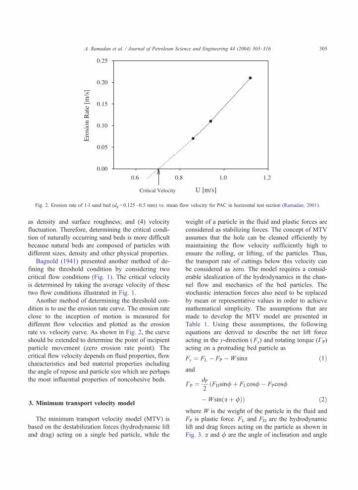
Fig. 2. Erosion rate of 1-l sand bed (dp = 0.125–0.5 mm) vs. mean flow velocity for PAC in horizontal test section (Ramadan, 2001).

A. Ramadan et al. / Journal of Petroleum Science and Engineering 44 (2004) 303–316 305

as density and surface roughness; and (4) velocity

fluctuation. Therefore, determining the critical condi-

tion of naturally occurring sand beds is more difficult

because natural beds are composed of particles with

different sizes, density and other physical properties.

Bagnold (1941) presented another method of de-

fining the threshold condition by considering two

critical flow conditions (Fig. 1). The critical velocity

is determined by taking the average velocity of these

two flow conditions illustrated in Fig. 1.

Another method of determining the threshold con-

dition is to use the erosion rate curve. The erosion rate

close to the inception of motion is measured for

different flow velocities and plotted as the erosion

rate vs. velocity curve. As shown in Fig. 2, the curve

should be extended to determine the point of incipient

particle movement (zero erosion rate point). The

critical flow velocity depends on fluid properties, flow

characteristics and bed material properties including

the angle of repose and particle size which are perhaps

the most influential properties of noncohesive beds.

3. Minimum transport velocity model

The minimum transport velocity model (MTV) is

based on the destabilization forces (hydrodynamic lift

and drag) acting on a single bed particle, while the

weight of a particle in the fluid and plastic forces are

considered as stabilizing forces. The concept of MTV

assumes that the hole can be cleaned efficiently by

maintaining the flow velocity sufficiently high to

ensure the rolling, or lifting, of the particles. Thus,

the transport rate of cuttings below this velocity can

be considered as zero. The model requires a consid-

erable idealization of the hydrodynamics in the chan-

nel flow and mechanics of the bed particles. The

stochastic interaction forces also need to be replaced

by mean or representative values in order to achieve

mathematical simplicity. The assumptions that are

made to develop the MTV model are presented in

Table 1. Using these assumptions, the following

equations are derived to describe the net lift force

acting in the y-direction (Fy) and rotating torque (CP)

acting on a protruding bed particle as

Fy ¼ FL � FP �W sina ð1Þand

CP ¼ dP

2ðFDsin/ þ FLcos/ � FPcos/

�W sinða þ /ÞÞ ð2Þwhere W is the weight of the particle in the fluid and

FP is plastic force. FL and FD are the hydrodynamic

lift and drag forces acting on the particle as shown in

Fig. 3. a and / are the angle of inclination and angle

Table 1

Basic assumption in the MTV model

Bed Particles Fluid velocity

Uniform thickness uniform size no fluctuation

Void-free collision-free

Stationary uniform density

spherical


of repose, respectively. P is a contact point with a

neighboring particle and considered as the axis of

rotation during rolling. Rolling is not the only mech-

anism for initiating the movement of the bed particles.

A bed particle may start its motion in the direction

normal to the bed plane depending on the flow

condition, bed properties and geometric parameters.

The lifting of bed particles occurs when the lift

force overcomes the plastic force and gravity in the

direction of lift. Consequently, the critical condition

for initiating particle lifting is when the net lift force is

zero (Fy= 0). Similarly, the net rotating torque must be

zero to initiate rolling of the bed particles. Therefore, it

is necessary to model forces involved in dislodging the

protruding particle in order to determine the critical

Fig. 3. Forces acting on a single bed particle at an active erosion site.

velocity. The modeling equations for these forces are

listed in Table 2. Details of these model equations and

the factors ( fL and fD) used in the lift and drag force

equations were published by Ramadan et al. (2001).

The influence of drag reduction on the drag coeffi-

cient (CD) must be considered for drag-reducing fluids.

Therefore, the drag coefficient must be modified to

account for drag reduction when the particles Reynolds

number is greater than 0.1. Choi and John (1996)

presented an empirical relationship between the drag-

reduction efficiency and polymer solution properties

for both water- and oil-soluble polymers. Thus, the

universal correlation between the polymer concentra-

tion, C, and drag reduction (DR) in percent is

C

DR¼ KC*

DRmax

þ C

DRmax

ð3Þ

where C*, K and DRmax are empirical constants that

depend on the polymer–solvent system.

Several studies have been conducted to determine

the extent of drag reduction for different polymers.

Sohn et al. (2001) studied drag reduction properties of

xanthan gum using a rotating disk apparatus. The

dependency of drag reduction on various factors,

including polymer molecular weight, polymer concen-

tration and temperature, were investigated. The result

indicated that the polymer concentration significantly

affects the drag reduction behavior of xanthan gum

solutions at low concentrations ( < 100 ppm). In addi-

tion, they found the empirical constants for Eq. 3.

Using their constants, the equation for drag reduction is

DR ¼ C

0:0354C þ 4� 10�5ð4Þ

where DR is drag reduction in percent, and C is the

mass fraction of the polymer.

Table 2

Model equations used in Eqs. 1 and 2

Force Equation

Lift FL ¼ 1:615l ud2p

m0:5fL

du

dy

� �0:5

¼ KLu2

Drag FD ¼ 1

2CDq u2ApfD ¼ KDu

2

Weight W ¼ p6d3pðqs � qf Þg

Plastic FP ¼pd2psy2

/ þ ðp=2� /Þsin2/ � cos/sin/� �


Using the estimates for the drag and lift forces,

equations in Table 2 may be substituted into Eqs. 1

and 2 to obtain the two critical velocities of a cuttings

bed as

uL ¼

ffiffiffiffiffiffiffiffiffiffiffiffiffiffiffiffiffiffiffiffiffiffiffiffiffiffiffiffiFP þW sinðaÞ

KL

sð5Þ

and

uR ¼

ffiffiffiffiffiffiffiffiffiffiffiffiffiffiffiffiffiffiffiffiffiffiffiffiffiffiffiffiffiffiffiffiffiffiffiffiffiffiffiffiffiffiffiffiffiffiffiffiffiffiFPcosð/Þ þW sinða þ /Þ

KDDRsinð/Þ þ KL

sð6Þ

where uL and uR are critical velocities for lifting and

rolling, respectively. An iterative procedure is neces-

sary to solve Eqs. 5 and 6, because KL is a function of

the local velocity (u). The calculated velocities are the

local velocities at the center of a bed particle. If the

two calculated values are different, the lower value is

the critical velocity. Using the velocity profile, the

mean flow velocity can be determined from the local

velocity. In turbulent flow, the near-bed velocity

profile is often described by the law of the wall (See

Appendix A). Several forms of this law have been

suggested; however, the law is often represented by

different expressions in different flow regions that are

presented in Fig. 4.

Fig. 4. Dimensionless velocity profiles of water and 0.2%

To apply the law of the wall to a Bingham fluid, it

is necessary to use the effective viscosity instead of

the Newtonian viscosity. In the case of power-law

fluids, use of the effective viscosity in the calculation

of near-bed velocity profiles does not yield accurate

result. Therefore, the law of the wall has to be

modified for power-law fluids. Szilas et al. (1981)

developed the law of the wall for power-law fluids.

Nonetheless, the law of the wall, which is obtained

from regular fluids, cannot be used for solutions of

drag-reducing polymers; experimental studies on fully

developed turbulent pipe flow of drag-reducing poly-

mer solutions indicated that the velocity profile is

significantly affected by drag reduction (Escudier et

al., 1999; Hoyer and Gry, 1996).

Fig. 4 compares dimensionless velocity profiles of

a 0.2 % xanthan gum solution to water (Escudier et

al., 1999). The figures indicate that drag-reducing

polymers significantly affect the law of the wall. It

is apparent from the figures that the velocity profile in

the viscous sublayer ( y+ < 5) is not influenced by the

addition of the polymer; however, the buffer zone and

logarithmic layer are considerably affected. The buffer

zone increases in thickness with increasing levels of

drag reduction. This results in high flow velocity in

the logarithmic layer, which is responsible for the

increase in the flow rate with the introduction of drag-

xanthan gum solution (from Escudier et al., 1999).


reducing polymers (Virk, 1975). The measured velo-

city profile roughly matches Virk’s curve.

The change in velocity profile significantly alters

the turbulent friction factor. According to Escudier et

al. (1999), the reduction in the turbulent friction factor

is as high as 50% for Reynolds numbers between

4000 and 50,000. Shenoy and Mashelkar (1983)

developed a specific friction factor correlation for

drag-reducing fluids as f = a/Reb, where a = 0.42 and

b = 0.55 (Shenoy, 1986).

Flow regime is another factor in determining the

critical flow velocity of drag-reducing fluids; since the

drag reduction phenomena is restricted to turbulent

flow. Therefore, it is important to accurately deter-

mine the critical Reynolds number. Hanks and Pratt

(1967) presented commonly used turbulent criteria for

Bingham fluids; they found that the Hedstrom number

(NHe) could roughly be correlated with the critical

Reynolds number, Rec by (Bourgoyne et al., 1986)

logRec ¼ 0:027ðlogNHeÞ2 þ 0:045logNHe þ 2:93

ð7Þ

where the Hedstrom number (NHe) is given as qfsyD2/

lp2. Although this method is a promising turbulent

criterion for Bingham fluids, it may not be applied to

drag-reducing fluids. Escudier et al. (1999) provided

extensive sets of experimental data for turbulent pipe

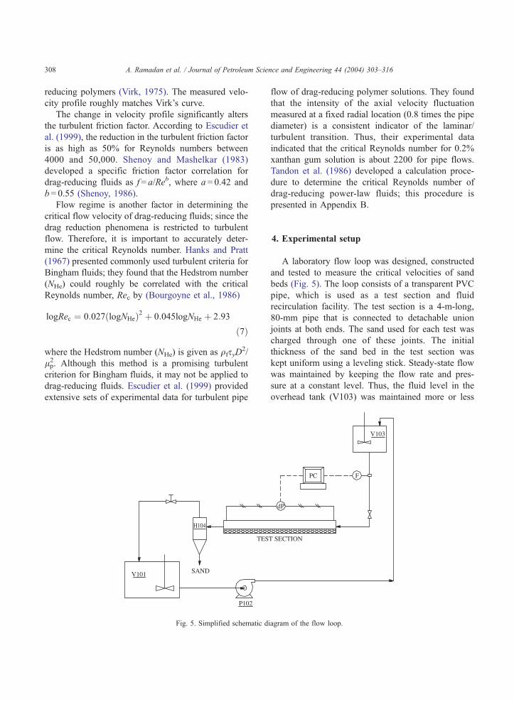
Fig. 5. Simplified schematic d

flow of drag-reducing polymer solutions. They found

that the intensity of the axial velocity fluctuation

measured at a fixed radial location (0.8 times the pipe

diameter) is a consistent indicator of the laminar/

turbulent transition. Thus, their experimental data

indicated that the critical Reynolds number for 0.2%

xanthan gum solution is about 2200 for pipe flows.

Tandon et al. (1986) developed a calculation proce-

dure to determine the critical Reynolds number of

drag-reducing power-law fluids; this procedure is

presented in Appendix B.

4. Experimental setup

A laboratory flow loop was designed, constructed

and tested to measure the critical velocities of sand

beds (Fig. 5). The loop consists of a transparent PVC

pipe, which is used as a test section and fluid

recirculation facility. The test section is a 4-m-long,

80-mm pipe that is connected to detachable union

joints at both ends. The sand used for each test was

charged through one of these joints. The initial

thickness of the sand bed in the test section was

kept uniform using a leveling stick. Steady-state flow

was maintained by keeping the flow rate and pres-

sure at a constant level. Thus, the fluid level in the

overhead tank (V103) was maintained more or less

iagram of the flow loop.

Fig. 6. Relationship between apparent viscosity and shear rate for PAC and 0.2% xanthan gum solutions.

Table 3

Average critical velocities for water tests in a horizontal pipe

Particle size

range (mm)

Average

particle

size (mm)

Sand

volume (l)

Critical

velocity

(m/s)

0.125–0.5 0.31 1.00 0.2567

0.5–1.2 0.85 1.00 0.3157

2.0–3.5 2.75 1.00 0.5057

4.5–5.5 5.00 1.00 0.5675

0.125–0.5 0.31 2.50 0.2700

0.5–1.2 0.85 2.50 0.3133

2.0–3.5 2.75 2.50 0.5000

0.125–0.5 0.31 4.00 0.2500

0.5–1.2 0.85 4.00 0.2850

2.0–3.5 2.75 4.00 0.5000


constant during the test runs. This was achieved with

a centrifugal pump (P102) that was used to recycle

the fluid from the circulation tank (V101) to the

overhead tank (V103). The regulated pump operated

between maximum and minimum levels of the over-

head tank.

The magnetic flowmeter (F) and differential pres-

sure transmitter (dP) were used to measure the flow

rate and pressure drop across the test section. Both

were connected to a PC to display and record the data.

The hydrocyclone (H104) was placed downstream of

the test section to separate sand from the fluid and

thus avoid sand recirculation.

Aqueous solutions of 0.1% polyanionic celluose

(PAC) and 0.2% xanthan gum (XG) were prepared in

the circulation tank. A variable speed agitator was

used to maintain the homogeneity of the solution. The

temperature of the fluid was maintained at 20 jC with

electric heaters at the bottom of the vessel. A manu-

ally operated valve downstream of the test section was

used to regulate the flow rate.

The critical velocities of the sand beds were

measured using the Bagnold’s threshold criteria.

The subjectivities of the measurements were mini-

mized by isolating the person who detected the

critical conditions from the operator. Each experi-

ment involved the following procedures: (1) filling

of the test section with the sand sample; (2) keeping

a uniform bed thickness across the length of the

channel; and (3) measuring the rheology and tem-

perature of the fluid. The rheologies of the solutions

are presented in Fig. 6.

5. Test result

The experimental test runs indicated that the

most exposed particles to the flow begin to vibrate

and move when the flow velocity reaches the

critical velocity. As the flow velocity increases, the

hydrodynamic forces drag the bed particles along.

Table 4

Critical velocities for water tests in a 78j inclined pipe

Particle size

range (mm)

Average

particle

size (mm)

Sand

volume (l)

Critical

velocity

(m/s)

0.125–0.5 0.31 1.00 0.2800

0.125–0.5 0.31 1.00 0.2500

0.5–1.2 0.85 1.00 0.3000

0.5–1.2 0.85 1.00 0.3200

2.0–3.5 2.75 1.00 0.5300

2.0–3.5 2.75 1.00 0.5100

Table 6

Measured critical velocities for XG tests in a horizontal pipe

Particle size

range (mm)

Average

particle

size (mm)

Sand

volume (l)

Critical

velocity

(m/s)

0.125–0.5 0.31 6.00 0.48

0.5–1.2 0.85 4.00 1.00

0.5–1.2 0.85 6.00 1.01

2.0–3.5 2.75 4.00 0.77

2.0–3.5 2.75 6.00 0.93

4.5–5.5 5.0 4.00 0.89


As a result, the particles start moving mostly by

rolling over the surface the bed. Moreover, it was

apparent that there exists a unique critical velocity

above which bed particles can be kept in full

suspension.

Tables 3 and 4 present critical velocities of water

test runs at 90j (horizontal) and 78j of inclinations.

The tests were conducted using different bed size

ranges and bed thickness. The result indicates that

the critical velocity increases as particle size

increases and slightly decreases as the sand volume

(bed thickness) increases. The critical velocity is

sensitive to particle diameter for fine particles. The

critical velocities presented in Table 3 are average

critical velocities. The average critical velocity is

defined as the mean value of critical velocities

Table 5

Measured critical velocities for PAC test in a horizontal pipe

Particle size

range (mm)

Average

particle

size (mm)

Sand

volume (l)

Critical

velocity

(m/s)

0.125–0.5 0.31 1.00 0.53

0.125–0.5 0.31 1.00 0.51

0.125–0.5 0.31 1.00 0.49

0.5–1.2 0.85 1.00 0.65

0.5–1.2 0.85 1.00 0.74

0.5–1.2 0.85 1.00 0.62

0.5–1.2 0.85 1.00 0.70

2.0–3.5 2.75 1.00 0.51

2.0–3.5 2.75 1.00 0.56

2.0–3.5 2.75 1.00 0.56

2.0–3.5 2.75 1.00 0.53

2.0–3.5 2.75 1.00 0.56

4.5–5.5 5.00 1.00 0.55

4.5–5.5 5.00 1.00 0.55

4.5–5.5 5.00 1.00 0.52

4.5–5.5 5.00 1.00 0.53

measured under identical test conditions. This was

done to determine the accuracy and reproducibility

of measurements. Statistical analysis indicated that

the measurements are reproducible within F 3% at

90% degree of confidence.

As it is anticipated, the critical velocity of the beds

increases slightly with the angle of inclination. Com-

parison of the results in Tables 3 and 4 shows that the

effect of angle of inclination is negligible at angles

close to horizontal. Similarly the results of the PAC

test are presented in Table 5. All of the tests were

performed using 1 liter of sand bed.

The critical velocity result of xanthan gum is

shown in Table 6. Unlike the water and PAC tests,

the test runs using xanthan gum were conducted with

higher sand volumes, because the critical velocity for

1 l of sand bed is more than the maximum velocity

obtained by a gravity flow. As a result, xanthan gum

tests were conducted with 4 and 6 l of sand in the

beds.

6. Comparison of experimental result with model

predictions

Figs. 7 and 8 compare the model predictions

with the test result for water in horizontal and

inclined test sections. There is no significant dif-

ference in the critical velocity values between the

horizontal and inclined cases. It is apparent from

Fig. 8 that the model predictions for the inclined

test section show satisfactory agreement with the

measured data. However, the model predictions

indicate change in pattern of critical velocity curve

as the particle size approaches 0.8 mm, which is

the result of the interaction between the bed

Fig. 7. Comparison of model predictions with measured data for

water tests in a horizontal pipe.


particles and the velocity field. As shown in Fig. 4,

the velocity profile near the bed has three different

layers: (1) the viscous sublayer; (2) the buffer

zone; and (3) the logarithmic layer. The bed

particles have the chance to be inside any of these

layers depending on the hydrodynamics of the flow

and the size of the particle. As a result, when a

particle is in the viscous sublayer, the local veloc-

ity becomes too small to initiate the movement of

the particles. Detailed result from the model indi-

Fig. 8. Comparison of model predictions with the m

cated that particles larger than 0.8 mm are not fully

submerged in the viscous sublayer. Instead, they

get the chance of being dragged by the action of

the strong local velocity. Hence, for particles larger

than the viscous sublayer thickness, as the particle

size increases, the change in the local velocity

becomes relatively little and does not compensate

for simultaneous inertial variation (change in the

mass of the particle). Consequently, the critical

velocity rises with increasing particle size. For

particles less than 0.8 mm, the model predictions

show that the critical velocity decreases as the

particle size increases. Pervious experimental stud-

ies (Hjulstrom, 1935) on critical velocity of fine

sand also supports this prediction.

The critical velocity test results and predictions of

the model for PAC are presented in Fig. 9. The

model predictions show satisfactory agreement with

the measured data. The pattern of the test data for

water is significantly different from that of the PAC

solution. For PAC test runs, the critical velocity

decreases, as the particles become coarser, beginning

approximately from 0.8 mm. As stated previously,

the existence of such patterns in the critical velocity

curves has a hydrodynamic explanation. The viscous

sublayer thickness in the case of PAC is much thicker

than that of water. As a result, the protruding

easured data for water in a 78j inclined pipe.

Fig. 9. Model prediction and measured critical velocities in a horizontal pipe for PAC.


particles are inside the viscous sublayer where the

velocity gradient is high enough to compensate for

the inertial change that arises from the coarsening of

the particles. Consequently, a lower critical velocity

is required when the particles become coarser within

the viscous sublayer. When bed particles become too

Fig. 10. Model prediction and measured critical velocities in a h

small (i.e. less than 0.5 mm), increasing the particle

size does increase the critical velocity. This is prin-

cipally due to the weakening of the pressure drag for

noninertial particles. As a result, the increase in local

velocity does not compensate for the inertial change.

For such small bed particles, the movement is initi-

orizontal pipe for xanthan gum, assuming turbulent flow.

Fig. 11. Model prediction and measured critical velocities in a horizontal pipe for xanthan gum, assuming laminar flow.


ated by the shearing action of the fluid. Therefore,

the tiny particles need a lower mean critical velocity

than the coarse ones in this range.

Experimentally measured critical velocities for

xanthan gum solution are shown in Fig. 10 together

Fig. 12. Model prediction and measured critical vel

with the model predictions, which are obtained by

assuming that the flow is turbulent. The pattern of

critical velocity curves for xanthan gum and PAC

solutions is very similar; however, the discrepancies

between the model predictions and the measured ones

ocities in a horizontal pipe for xanthan gum.


are relatively high. This variation may be due to the

turbulent flow assumption, because both critical ve-

locity curves are almost below the constant velocity

lines that correspond to the critical Reynolds numbers.

The critical Reynolds numbers for the test runs were

about 1500 using Hanks criteria; however, Escudier et

al. (1999) found that the critical Reynolds number for

0.2 % xanthan gum solution in pipe flow is about

2200. Hence, the result must be searched by assuming

the flow to be laminar flow.

Fig. 11 shows the model predictions based on

laminar flow together with the measured result. In

this case, the model predictions show better agree-

ment with the measured data. Nevertheless, the

laminar assumption is not exact, because the curves

are not completely below the constant velocity lines

that correspond to the critical Reynolds numbers.

Both the critical velocity curves are above the

constant velocity lines obtained from Hanks correla-

tion. This implies that applying Hanks correlation

reduces the predicted critical velocities by about

20%. More reasonable values of critical velocity

predictions can be obtained by using a measured

critical Reynolds number or appropriate correlation.

If the critical Reynolds number is assumed to be

2200, the critical velocity curve for the 4-l case has

to follow the constant velocity curve for particles

greater than 1 mm, because the flow beyond 0.77 m/

s is no longer laminar. Hence, it is necessary to use

the critical velocity obtained by assuming turbulent

flow; however, the model-predicted critical velocity

for turbulent flow actually does not give turbulent

flow as shown in Fig. 10. Understandably, the

critical velocity has to satisfy the model equations

and the flow regime assumption. The constant ve-

locity line (Rec = 2200) simultaneously satisfies these

two conditions for particles greater than 1 mm. This

means that keeping the flow regime in a turbulent

condition is sufficient to transport particles greater

than 1 mm for this case.

The model prediction assuming Rec = 2200 and

adopting the model for flow regime inconsistency

is presented in Fig. 12. The figures indicate that

the model prediction curves follow the pattern of

the experimental data with a maximum deviation of

about 25%. For the 4-l case, model predictions

indicate that the particles with diameters less than 5

mm are completely in the viscous sublayer.

7. Conclusions

� Model predictions of critical velocities are in

good agreement with experimentally measured

data. The existence of different patterns in the

critical velocity curves is the result of the

interaction of the bed particles with the velocity

field, which is highly dependent on the location

of a protruding bed particle relative to the

hydrodynamic layers.� The mechanistic transport velocity model can be

used to analyze cuttings transport abilities of drag-

reducing drilling fluids; however, it is necessary to

account for the change in (1) velocity profile, (2)

friction factor, (3) drag coefficient and (4) critical

Reynolds number.� In turbulent flows, the actual critical velocity is

the maximum of the critical velocity obtained

using the traditional MTV model and the

velocity required to attain the turbulent flow

regime.� Small diameter wells require a lower critical

transport velocity than the large ones; however,

this variation in critical velocity is insignificant for

fluids with low viscosity.

Nomenclature

C concentration

CD drag coefficient

C* empirical constant

dp particle diameter

DR drag reduction in percent

DRmax maximum drag reduction

fD drag coefficient correction factor

fL lift coefficient correction factor

FP plastic force

FD drag force

FL lift force

Fy net force on the particle acting in the

direction of y-axis

k consistency index

n power-law exponent

K empirical constant

NHe Hedstrom number

PAC polyanionic celluose

Re pipe Reynolds number

Rep particle Reynolds number


Rec critical Reynolds number

t time

u local flow velocity

U mean flow velocity of the fluid

Uc,1 upper critical flow velocity of the fluid

Uc,2 lower critical flow velocity of the fluid

us friction velocity

u+ dimensionless local velocity

uR critical local flow velocity for rotating bed

particles

uL critical local flow velocity for lifting bed

particles

W weight of the particle in the fluid

x axial coordinate

XG xanthan gum

y coordinate normal to the flow

y+ dimensionless distance from the wall

Greek Symbols

a angle of inclination

/ angle of repose

l apparent viscosity

lp plastic viscosity

lw viscosity of water

qf density of the fluid

qs density of the particle

qw density of water

sw wall shear stress

sy yield strength of the fluid

m kinematic viscosity

CP rotating torque on a particle

Acknowledgements

The authors express their appreciation to the staff

of the workshop and the laboratory at the Department

of Petroleum Engineering and Applied Geophysics,

NTNU for their assistance in building the flow loop.

The work was financed by Statoil, and we thank them

for their support.

Appendix A. Law of the Wall

A formulation of the law of the wall that is valid

throughout the viscous sublayer as well as through the

turbulent boundary layer was published by Launder

and Spalding (1974):

yþ ¼ uþ þ Aðej uþ � 1� j uþ � 1

2ðj uþÞ2

� 1

6ðj uþÞ3 � 1

24ðj uþÞ4 ðA-1Þ

where A is 0.1108, j is 0.4, y+ is the dimensionless

distance from the wall and u+ is dimensionless local

velocity. Dimensionless distance and velocity are

calculated as follows:

yþ ¼ yus

mðA-2Þ

uþ ¼ u

usðA-3Þ

where y is the distance from the wall, u is local velocity

and us is friction velocity given by (sw/qf)0.5, where

sw is the wall shear stress.

Using an elastic sublayer model, Virk (1975)

developed an expression for the velocity profile of

drag-reducing fluids. The elastic sublayer is assumed

to exist between the viscous and logarithmic layers.

Thus, the formulation of the law of the wall for a drag-

reducing fluid is

uþ ¼ yþ; for viscous subplayer ð0VyþV10Þ ðA-4aÞ

uþ ¼ 11:7lnyþ � 17;

for elastic subplayer ð10VyþV50Þ ðA-4bÞ

uþ ¼ 2:5lnyþ þ 20:3;

for logarithmic layer ðyþz50Þ ðA-4cÞ

Appendix B. Critical Reynolds number

The critical Reynolds number of drag-reducing

power-law fluids is given by ReC = u*qfD, where u*

is given by (Tandon et al., 1986)

u* ¼ 1

3nþ 1b

D

2

� �1�n2�n

u1

2�no ðA-5Þ


where b is given by

b ¼ wn1�nðnþ 2Þnþ2nþ1

h i1=ð2�nÞðA-6Þ

where w = 4qf k/(31.5qwlw) and uo denotes the mean

flow velocity at the critical Reynolds number for

water.

References

Bagnold, R.A., 1941. The Physics of Blow Sand and Desert Dunes.

Chapman and Hall, Methuen, pp. 200–256.

Bourgoyne, A.T., Millheim, K.K., Chenvert, M.E., Young,

F.S., 1986. Applied Drilling Engineering. SPE Text book,

Richardnson, pp. 144–160.

Choi, H.J., John, M.S., 1996. Polymer-induced turbulent drag re-

duction. Ind. Eng. Chem. Res. 35, 2993–2998.

Clark, R.K., Bickham, K.L., 1994. A Mechanistic model for cut-

tings transportation. SPE 28306, 69th Ann. Tech. Conf., New

Orleans.

Escudier, M.P., Presti, F., Smith, S., 1999. Drag reduction in the

turbulent pipe flow of polymers. J. Non-Newton. Fluid Mech.

81, 197–213.

Hanks, R.W., Pratt, D.R., 1967. On the flow of bingham plastic

slurries in pipes and between parallel plates. Trans. AIME 240,

342–346.

Henderson, F.M., 1966. Open Channel Flow. Macmillan Series,

New York, pp. 405–485.

Hjulstrom, F., 1935. Studies of the morphological activity of

river Fyris. Geological Institute of Uppsala Bulletin, XXV,

pp. 221–527.

Hoyer, K., Gry, A., 1996. Turbulent velocity field in heterogeneous-

ly drag reduced pipe flow. J. Non-Newton. Fluid Mech. 65,

221–240.

Launder, B.E., Spalding, D.B., 1974. The numerical computation

of turbulent flows. Comput. Methods Appl. Mech. Eng. 3,

269–289.

Ramadan, A., 2001. Mathematical modelling and experimental in-

vestigation of solids and cuttings transport. PhD Thesis, Norwe-

gian University of Science and Technology, Trondheim.

Ramadan, A., Skalle, P., Johansen, S.T., Sveen, J., Saasen, A.,

2001. Mechanistic model for cuttings removal from solid bed

in inclined channels. J. Pet. Sci. Eng. 30, 3–4.

Shenoy, A.V., 1986. Turbulent flow velocity profile in drag-re-

ducing fluids. Encyclopedia of Fluid Mechanics, vol. 7. Gulf

Publishing, Houston, pp. 479–503.

Shenoy, A.V., Mashelkar, R.A., 1983. Engineering estimate of hy-

drodynamic entrance lengths in non-Newtonian turbulent flow.

Ind. Eng. Chem. Process Des. Dev. 22, 165–168.

Sohn, J.I., Kim, C.A., Choi, H.J., John, M.S., 2001. Drag reduction

effectiveness of xanthan gum in a rotating disk apparatus. Car-

bohydr. Polym. 45, 61–68.

Szilas, A.P., Bobok, E., Navratil, L., 1981. Determination of turbu-

lent pressure loss of non-Newtonian oil flow in rough pipes.

Rheol. Acta 20 (5), 487–496.

Tandon, P.N., Kulshreshtha, A.K., Agarwal, R., 1986. Rheology

study of laminar-turbulent transition in drag-reducing polymeric

solutions. Encycl. Fluid Mech. 5, 459–477.

Virk, P.S., 1975. Drag reduction fundamentals, journal review.

AIChE J. 21, 625–656.

Application of the minimum transport velocity model for drag-reducing polymers

Documents