Chapter 2 Application of MATLAB/SIMULINK in Solar PV Systems Learning Objectives On completion of this chapter, the reader will have knowledge on: • Basic components of Solar PV system and its merits and demerits. • Involvement of power electronic devices in Solar PV components. • MATLAB/SIMULINK model of different control strategies of power conditioning unit. • Importance of MATLAB/SIMULINK model in improving the efficiency of the overall solar PV system. • Characteristics of Solar PV panel and its MATLAB/SIMULINK model. • Characteristics and MATLAB/SIMULINK model of Solar PV power conditioning unit. MATLAB and Power electronics application ranges from power supplies to robotic controls, industrial automation, automotive, industrial drives, power quality, and renewable energy systems. In particular, before the installation of power plant, MATLAB finds applications in selecting the system based on the requirements and to choose particular components for the Solar PV application. This chapter is to explore the role and possibility of MATLAB along with its tool boxes in Solar PV Systems to promote Modeling, and Simulation with emphasis on Analysis, and Design. In renewable energy systems applications, MATLAB helps for selecting the matrix manipulations in the converters to grid inverter, plotting of functions and data, implementation of MPPT algorithms, creation of user interfaces for monitor- ing the Solar PV modules and for interfacing with inverters and converters, wherein which control algorithms would be written in other languages. As a result of the MATLAB simulation of the components of the solar PV system one can benefit from this model as a photovoltaic generator in the framework of the MATLAB/ SIMULINK toolbox in the field of solar PV power conversion systems. In addition, © Springer International Publishing Switzerland 2015 S. Sumathi et al., Solar PV and Wind Energy Conversion Systems, Green Energy and Technology, DOI 10.1007/978-3-319-14941-7_2 59

Welcome message from author
This document is posted to help you gain knowledge. Please leave a comment to let me know what you think about it! Share it to your friends and learn new things together.
Transcript

Chapter 2
Application of MATLAB/SIMULINKin Solar PV Systems
Learning Objectives
On completion of this chapter, the reader will have knowledge on:
• Basic components of Solar PV system and its merits and demerits.
• Involvement of power electronic devices in Solar PV components.
• MATLAB/SIMULINK model of different control strategies of power
conditioning unit.
• Importance of MATLAB/SIMULINK model in improving the efficiency
of the overall solar PV system.
• Characteristics of Solar PV panel and its MATLAB/SIMULINK model.
• Characteristics and MATLAB/SIMULINK model of Solar PV power
conditioning unit.
MATLAB and Power electronics application ranges from power supplies to robotic
controls, industrial automation, automotive, industrial drives, power quality, and
renewable energy systems. In particular, before the installation of power plant,
MATLAB finds applications in selecting the system based on the requirements and
to choose particular components for the Solar PV application. This chapter is to
explore the role and possibility of MATLAB along with its tool boxes in Solar PV
Systems to promote Modeling, and Simulation with emphasis on Analysis, and
Design. In renewable energy systems applications, MATLAB helps for selecting
the matrix manipulations in the converters to grid inverter, plotting of functions and
data, implementation of MPPT algorithms, creation of user interfaces for monitor-
ing the Solar PV modules and for interfacing with inverters and converters, wherein
which control algorithms would be written in other languages. As a result of the
MATLAB simulation of the components of the solar PV system one can benefit
from this model as a photovoltaic generator in the framework of the MATLAB/
SIMULINK toolbox in the field of solar PV power conversion systems. In addition,
© Springer International Publishing Switzerland 2015
S. Sumathi et al., Solar PV and Wind Energy Conversion Systems,Green Energy and Technology, DOI 10.1007/978-3-319-14941-7_2
59

such models discussed in this chapter would provide a tool to predict the behavior
of solar PV cell, module and array, charge controller, SOC battery, inverter, and
MPPT, under climate and physical parameters changes.
2.1 Basics of Solar PV
A photovoltaic system is made up of several photovoltaic solar cells. An individual
small PV cell is capable of generating about 1 or 2 W of power approximately
depends of the type of material used. For higher power output, PV cells can be
connected together to form higher power modules. In the market the maximum
power capacity of the module is 1 kW, even though higher capacity is possible to
manufacture, it will become cumbersome to handle more than 1 kW module.
Depending upon the power plant capacity or based on the power generation,
group of modules can be connected together to form an array.
Solar PV systems are usually consists of numerous solar arrays, although the
modules are from the same manufactures or from the same materials, the module
performance characteristics varies and on the whole the entire system performance
is based on the efficiency or the performance of the individual components.
Apart from the solar PV module the system components comprises a battery
charge controller, an inverter, MPPT controller and some of the low voltage
switchgear components. Presently in the market, power conditioning unit consists
of charge controller, inverter and MPPT controller. A Balance-of-System (BoS)
includes components and equipments that convert DC supply from the solar PV
module to AC grid supply. In general, BOS of the solar PV system includes all
the components of the system except the Solar PV modules. In addition to
inverters, this includes the cables/wires, switches, enclosures, fuses, ground fault
detectors, surge protectors, etc. BOS applies to all types of solar applications
(i.e. commercial, residential, agricultural, public facilities, and solar parks).
In many systems, the cost of BOS equipment can equal or exceed the cost of the
PV modules. When examining the costs of PV modules, these costs do not include
the cost of BOS equipment. In a typical battery based solar PV system the cost of
the modules is 20–30 % of the total while the remaining 70 % is the balance of
systems (BOS). Apart from the 50 % of the system BOS costs a lot more mainte-
nance expense is also required for proper maintenance of the BOS. By controlling
the balance-of-system components, increase efficiency, and modernize solar PV
systems can be maintained. BOS components include the majority of the pieces,
which make up roughly 10–50 % of solar purchasing and installation costs, and
account for the majority of maintenance requirements. Thus, suitable integration of
the BOS is vital for the proper functionality and the reliability of the solar PV
system. However it is often completely overlooked and poorly integrated. Costs are
steadily decreasing with regard to solar panels and inverters.
As per the statistics, the Solar PV module world market is steadily growing at
the rate of 30 % per year. The reasons behind this growth are that the reliable
60 2 Application of MATLAB/SIMULINK in Solar PV Systems

production of electricity without fuel consumption anywhere there is light and the
flexibility of PV systems. Also the solar PV systems using modular technology and
the components of Solar PV can be configured for varying capacity, ranging from
watts to megawatts. Earlier, large variety of solar PV applications found to be in
industries but now it is being used for commercial as well as for domestic needs.
One of the hindrance factor is the efficiency of the solar PV cell, in the
commercial market a cell efficiency of up to 18.3 % is currently obtained,
depending on the technology that is used. When it is related to the module
efficiency, it is slightly lower than the cell efficiency. This is due to the blank
spaces between the arrays of solar cells in the module. The overall system efficiency
includes the efficiency and the performance of the entire components in the system
and also depends on the solar installation. Here there is another numerical drop in
value when compared to the module efficiency, this being due to conductance
losses, e.g., in cables. In the case of inverter, it converts the DC output from the
Solar PV module to the AC grid voltage with a certain degree of efficiency. It
depends upon conversion efficiency and the precision and quickness of the MPP
tracking called tracking efficiency. MPP tracking which is having an efficiency of
98–99 % is available in the market, each and every MPPT is based on a particular
tracking algorithm.
Current research states that all materials have physical limits on the electricity
that they can generate. For example, the maximum efficiency of crystalline silicon
is only 28 %. But tandem cells provide immense scope for development in coming
years. Efficiency of existing laboratory cells has already achieved efficiency values
of over 25 %. PV Modules with BOS components known as an entire PV system.
This system is usually sufficient to meet a particular energy demand, such as
powering a water pump, the appliances and lights in a home, and electrical
requirements of a community.
In the cost of PV systems and in consumer acceptance, reliability of PV arrays is
a crucial factor. With the help of fault-tolerant circuit design, reliability can be
improved using various redundant features in the circuit to control the effect of
partial failure on overall module yield and array power degradation. Degradation
can be limited by dividing the modules into a number of parallel solar cell networks.
This type of design can also improve module losses caused by broken cells. The
hot-spots in the Solar PV module can be avoided by having diodes across each cell
and that is called as bypass diodes. Practically a solar PV module consists of one
bypass diode for 18 cells to mitigate the effects of local cell hot-spots.
2.2 PV Module Performance Measurements
Peak watt rating is a key performance measurement of PV module. The peak watt
(Wp) rating is determined by measuring the maximum power of a PV module under
laboratory Standard Test Conditions (STC). These conditions related to the maxi-
mum power of the PV module are not practical. Hence, researchers must use the
2.2 PV Module Performance Measurements 61
NOCT (Nominal Operating Cell Temperature) rating. In reality, either of the
methods is designed to indicate the performance of a solar module under realistic
operating conditions. Another method is to consider the whole day rather than
“peak” sunshine hours and it is based on some of the factors like light levels,
ambient temperature, and air mass and also based on a particular application.
Solar arrays can provide specific amount of electricity under certain conditions.
In order to determine array performance, following factors to be considered:
(i) characterization of solar cell electrical performance (ii) degradation factors
related to array design (iii) assembly, conversion of environmental considerations
into solar cell operating temperatures and (iv) array power output capability. The
following performance criteria determines the amount of PV output.
Power Output Power output is represented in watts and it is the power available at
the charge controller/regulator specified either as peak power or average power
produced during one day.
Energy Output Energy Output indicates the amount of energy produced during a
certain period of time and it is represented in Wh/m2.
Conversion Efficiency It is defined as energy output from array to the energy
input from sun. It is also referred as power efficiency and it is equal to power output
from array to the power input from sun. Power is typically given in units of watts
(W), and energy is typical in units of watt-hours (Wh).
To ensure the consistency, safety and quality of Solar PV system components
and to increase consumer confidence in system performance IEEE, Underwriters
Laboratories (UL), International Electrotechnical Commission (IEC), AM0 Spec-
trum (ASTM) are working on standards and performance criteria for PV systems.
2.2.1 Balance of System and Applicable Standards
The market access requirements for PV equipment are segmented into safety and
performance. UL is a global leader in energy product testing and certification. The
focus of the UL standards is in providing requirements for materials, construction
and the evaluation of the potential electrical shock, fire safety hazard and also
testing and certification according to the appropriate energy standard. UL certifies
that PV equipment complies with the safety, environmental and other performance
requirements of the appropriate standards.
IEC focus on the requirements in terms and symbols, testing, design qualifica-
tion and type approval. UL supports manufacturers with the compliance to both the
UL and the IEC requirements. In addition, UL provides balance of systems equip-
ment certification to the standards identified in the diagram. These certifications
include materials (such as polymeric used for back sheets, encapsulates, and
adhesives), components (like junction boxes and connectors) and end-products
(for example, inverters and meters). Even though the design of solar PV system
62 2 Application of MATLAB/SIMULINK in Solar PV Systems
components can be done with the help of mathematical calculations or by using
dedicated software, there are certain protocols and standards in selecting the BOS
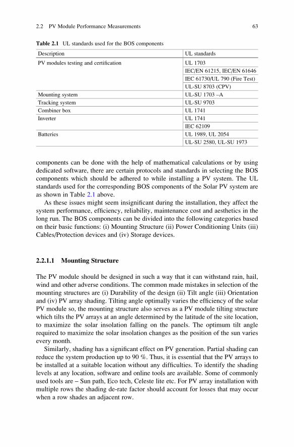
components which should be adhered to while installing a PV system. The UL
standards used for the corresponding BOS components of the Solar PV system are
as shown in Table 2.1 above.
As these issues might seem insignificant during the installation, they affect the
system performance, efficiency, reliability, maintenance cost and aesthetics in the
long run. The BOS components can be divided into the following categories based
on their basic functions: (i) Mounting Structure (ii) Power Conditioning Units (iii)
Cables/Protection devices and (iv) Storage devices.
2.2.1.1 Mounting Structure
The PV module should be designed in such a way that it can withstand rain, hail,
wind and other adverse conditions. The common made mistakes in selection of the
mounting structures are (i) Durability of the design (ii) Tilt angle (iii) Orientation
and (iv) PV array shading. Tilting angle optimally varies the efficiency of the solar
PV module so, the mounting structure also serves as a PV module tilting structure
which tilts the PV arrays at an angle determined by the latitude of the site location,
to maximize the solar insolation falling on the panels. The optimum tilt angle
required to maximize the solar insolation changes as the position of the sun varies
every month.
Similarly, shading has a significant effect on PV generation. Partial shading can
reduce the system production up to 90 %. Thus, it is essential that the PV arrays to
be installed at a suitable location without any difficulties. To identify the shading
levels at any location, software and online tools are available. Some of commonly
used tools are – Sun path, Eco tech, Celeste lite etc. For PV array installation with
multiple rows the shading de-rate factor should account for losses that may occur
when a row shades an adjacent row.
Table 2.1 UL standards used for the BOS components
Description UL standards
PV modules testing and certification UL 1703
IEC/EN 61215, IEC/EN 61646
IEC 61730/UL 790 (Fire Test)
UL-SU 8703 (CPV)
Mounting system UL-SU 1703 –A
Tracking system UL-SU 9703
Combiner box UL 1741
Inverter UL 1741
IEC 62109
Batteries UL 1989, UL 2054
UL-SU 2580, UL-SU 1973
2.2 PV Module Performance Measurements 63
2.2.1.2 Power Conditioners
In the off-grid inverter in a battery based PV system, it is important to review the
efficiency and the self-power consumption of the inverter along with the capacity,
power quality and surge rating. Generally inverter is normally sized to support the
load, power factor and surge. For the efficient operation of the inverter, it should
have low self consumption to increase the battery life. A high self consumption
inverter, continuously drains the battery which results in lower back up and
decrease the battery life cycle due to increased discharge. Further, as the efficiency
of the inverter changes with respect to the load, it is good practice to design the load
on average efficiency rather than the peak efficiency. In a typical inverter, the peak
efficiency is mostly between 20 % and 30 % of the total capacity.
2.2.1.3 Cables and Protection Devices
The main purpose of cabling is to allow a safe passage of current. Appropriate cable
sizing allows the current to be transferred within an acceptable loss limit to ensure
optimal system performance. In order to establish connection between solar PV
modules, charge controller, battery etc., cables are needed. The size of the cable
determined based on the transmission length, voltage, flowing current and the
conductor. The commonly found mistakes in installation sites are the undersized
or inappropriate selection of cables. The cables can be appropriately sized with the
help of several tools – such as mathematical formula, voltage drop tables and online
calculators. In addition to the appropriate sizing, selection of relevant type of wire is
also important in the case of solar PV application. For outdoor applications UV
stabilized cable must be used, while normal residential cables can be used in
indoors. This ensures the long term functioning of the cable and hence reduction
in the system ongoing maintenance.
2.2.1.4 Storage
For off-grid and critical applications, storage systems are required, the most
common medium of storage are the lead acid batteries. Presently researches are
going on in the field of Li-ion batteries and to implement the concept of fuel cells in
Solar PV Systems. One of the most expensive components in the PV system is the
battery. Under sizing the batteries will become more costly as the battery life cycle
is significantly reduced at higher Depth of Discharge (DOD%). At a higher depth of
discharge, expected average number of charge–discharge cycles of a battery
reduced. Further, a higher current discharge than the rating will dramatically reduce
the battery life. This can be avoided by carefully sizing of the battery according
to the ‘C-rating’ during the system design. It signifies the maximum amount of
current that can be safely withdrawn from the battery to provide adequate back up
and without causing any damage. A discharge more than the C-ratings, may cause
64 2 Application of MATLAB/SIMULINK in Solar PV Systems
irreversible capacity loss due to the fact that the rate of chemical reactions taking
place in the batteries cannot keep pace with the current being drawn from them.
The de-rating factor of the BOS plays a significance role in boosting up the
overall efficiency of the solar PV system. The de-rating factor can be calculated by
multiplying the BOS components de-rate factor. As per the survey, the overall
de-rating factor is 84.5 % at STC. With good selection and installation practice the
overall losses from BOS can be limited to 15.5 % at STC. With poor practice the
overall de-rate factor can be 54.7 % or even less, which means the losses can
account for more than 46 %.
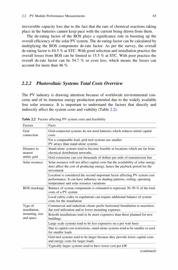
2.2.2 Photovoltaic Systems Total Costs Overview
The PV industry is drawing attention because of worldwide environmental con-
cerns and of its immense energy production potential due to the widely available
free solar resource. It is important to understand the factors that directly and
indirectly affect the system costs and viability (Table 2.2).
Table 2.2 Factors affecting PV system costs and feasibility
Factors Facts
Grid
connection
Grid-connected systems do not need batteries which reduces initial capital
costs
For a comparable load, grid-tied systems use smaller
PV arrays than stand-alone systems
Distance to
nearest
utility grid
Stand-alone systems tend to become feasible in locations which are far from
electrical distribution networks
Grid extensions can cost thousands of dollars per mile of transmission line
Solar resource Solar resource will not affect capital costs but the availability of solar energy
does affect the cost of producing energy, hence the payback period for the
investment
Location is considered the second important factor affecting PV system cost
performance. It can have influence on shading patterns, soiling, operating
temperature and solar resource variations
BOS (tracking) Balance of system components is estimated to represent 30–50 % of the total
costs of a PV system
Local safety codes or regulations can require additional balance of system
costs for the installation
Type of
installation,
mounting, size
and space
Commercial and industrial clients prefer horizontal Installation to maximize
flat roof utilization and to lower mounting expenses
Retrofit installations tend to be more expensive than those planned for new
buildings
Large scale systems tend to be less expensive on a per watt basis
Due to capital cost restrictions, stand-alone systems tend to be smaller or used
for smaller loads
Grid-tied systems tend to be larger because they provide lower capital costs
and energy costs for larger loads
Typically larger systems tend to have lower cost per kW
(continued)
2.2 PV Module Performance Measurements 65
2.3 Types of PV Systems
Based on the electric energy production, PV modules can be arranged into arrays to
increase electric output. Solar PV systems are generally classified based on their
functional and operational requirements, their component configurations. It can be
classified into grid-connected and stand-alone systems.
2.3.1 Grid-Connected Solar PV System
The primary component of grid-connected PV systems is power conditioning
unit (PCU). The PCU converts the DC power produced by the PV array into AC
power as per the voltage and power quality requirements of the utility grid.
A bi-directional interface is made between the PV system AC output circuits and
the electric utility network, typically at an on-site distribution panel or service
entrance. This allows the AC power produced by the PV system to either supply
on-site electrical loads or to back-feed the grid when the PV system output is greater
than the on-site load demand. This safety feature is required in all grid-connected
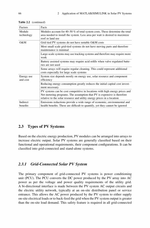
Table 2.2 (continued)
Factors Facts
Module
technology
Modules account for 40–50 % of total system costs. These determine the total
area needed to install the system. Less area per watt is desired to maximize
roof or land use
O&M Grid tied PV systems do not have notable O&M costs
Most small scale grid-tied systems do not have moving parts and therefore
maintenance is minimal
Large-scale systems may use tracking systems and therefore may require more
work
Battery assisted systems may require acid refills when valve regulated batte-
ries are not used
Some arrays will require regular cleaning. This could represent additional
costs especially for large scale systems
Energy use
and cost
System size depends mostly on energy use, solar resource and component
efficiency
Reducing energy consumption greatly reduces the initial capital cost invest-
ment necessary
PV systems can be cost competitive in locations with high energy prices and
Net metering programs. The assumption that PV is expensive is therefore
relative to the solar resource and utility energy prices in a location
Indirect
benefits
Emissions reductions provide a wide range of economic, environmental and
health benefits. These are difficult to quantify, yet they cannot be ignored
66 2 Application of MATLAB/SIMULINK in Solar PV Systems

PV systems, and ensures that the PV system will not continue to operate and
feed back into the utility grid when the grid is down for maintenance or during
grid failure state. Figure 2.1 shows the general block diagram of the grid connected
solar PV system. In grid-connected systems, switching of AC power from the
standby generator and the inverter to the service bus or the connected load is
accomplished by internal or external automatic transfer switches.
One of the important components of a grid-connected system is net metering.Standard service meters are odometer-type counting wheels that record power
consumption at a service point by means of a rotating disc, which is connected
to the counting mechanism. The rotating discs operate by an electro physical
principle called eddy current. Digital electric meters make use of digital electronic
technology that registers power measurement by solid-state current and voltage-
sensing devices that convert analog measured values into binary values that are
displayed on the meter using liquid crystal display (LCD) readouts.
Inverters are the main difference between a grid-connected system and a stand-
alone system. Inverters must have line frequency synchronization capability to
deliver the excess power to the grid. Net meters have a capability to record
consumed or generated power in an exclusive summation format. The recorded
power registration is the net amount of power consumed—the total power used
minus the amount of power that is produced by the solar power cogeneration
system. Net meters are supplied and installed by utility companies that provide
grid-connection service systems. Net metered solar PV power plants are subject to
specific contractual agreements and are subsidized by state and municipal govern-
mental agencies.
2.3.2 Stand-Alone Solar PV System
Stand-alone PV systems or direct coupled PV systems are designed and sized to
supply DC and/or AC electrical loads. It is called direct coupled systems because,
the DC output of a PV module or array is directly connected to a DC load. There is
no electrical energy storage (batteries) in direct-coupled systems as because of that,
the load only operates during sunlight hours. The maximum power point tracker
AC Load
Grid
Solar PVModule
DistributionPanel
PowerConditioning
Unit
Fig. 2.1 Bock diagram
of grid-connected solar
PV system
2.3 Types of PV Systems 67

(MPPT) is used between the array and load to help better utilize the available array
maximum power output and also for matching the impedance of the electrical load
to the maximum power output of the PV array. Figure 2.2 shows the general block
diagram of the stand alone solar PV system.
An example of direct coupled solar PV systems is in agriculture applications,
solar PV module can be directly connected to run the pump. Depending upon the
capacity of the pump, the module can be connected in series/parallel configurations.
In such application, surge protector is needed to be connected between the positive
and negative supply provides protection against lightning surges. Batteries are used
for energy storage in many stand-alone PV systems. Figure 2.3 shows the block
diagram of a typical stand-alone PV system powering DC and AC loads with
battery storage option.
The solar PV array configuration, a DC load with battery backup, is essentially
the same as the one without the battery except that there are a few additional
components that are required to provide battery charge stability. PV panels are
connected in series to obtain the desired increase in DC voltage, such as 12, 24, or
48 V. The charge controller regulates the current output and prevents the voltage
level from exceeding the maximum value for charging the batteries. The output of
the charge controller is connected to the battery bank by means of a dual DC cutoff
disconnect. Apart from this a cutoff switch can be provided, when turned off for
safety measures, disconnects the load and the PV arrays simultaneously.
During the sunshine hours, the load is supplied with DC power while simulta-
neously charging the battery. The controller will ensure that the DC power output
Solar PVModule DC / AC Load
Fig. 2.2 Direct coupled
solar PV system
Solar PV Array DC LoadCharge
Controller
Battery Inverter
AC Load
Fig. 2.3 Block diagram of stand-alone PV system with battery storage
68 2 Application of MATLAB/SIMULINK in Solar PV Systems

from the PV arrays should be adequate to sustain the connected load while sizing
the batteries. Battery bank sizing depends on a number of factors, such as the
duration of an uninterrupted power supply to the load when there is less or no
radiation from the sun. The battery bank produces a 20–30 % power loss due to heat
when in operation, which also must be taken into consideration. When designing a
solar PV system with a battery backup, the designer must determine the appropriate
location for the battery racks and room ventilation.
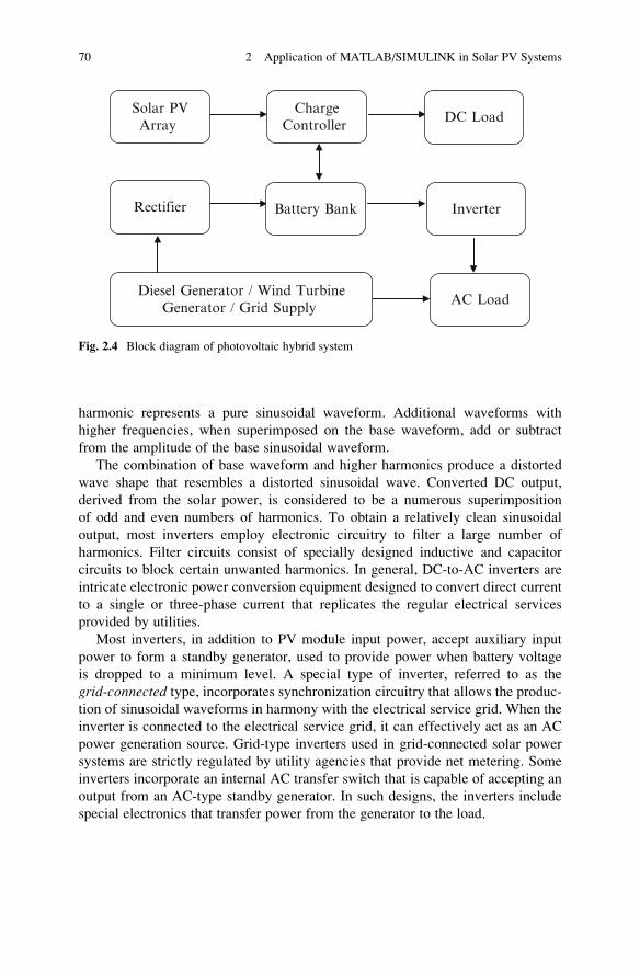
2.3.3 PV-Hybrid Systems
Hybrid systems generally refers to the combination of any two input sources, here
solar PV can be integrated with Diesel Generator, Wind Turbines, Bio-mass or any
other renewable on non-renewable energy sources. Solar PV systems will generally
use battery bank to store energy output from the panels to accommodate a
pre-defined period of insufficient sunshine, there may still be exceptional periods
of poor weather when an alternative source is required to guarantee power produc-
tion. PV-hybrid systems combine a PV module with another power sources -
typically a diesel generator, but occasionally another renewable supply such as a
wing turbine. The PV generator would usually be sized to meet the base load
demand, with the alternate supply being called into action only when essential.
This arrangement offers all the benefits of PV in respect of low operation and
maintenance costs, but additionally ensures a secure supply.
Hybrid systems can also be sensible approach in situations where occasional
demand peaks are significantly higher than the base load demand. It makes
little sense to size a system to be able to meet demand entirely with PV if, for
example, the normal load is only 10 % of the peak demand. By the same token, a
diesel generator-set sized to meet the peak demand would be operating at ineffi-
cient part-load for most of the time. In such a situation a PV-diesel hybrid would
be a good compromise. Figure 2.4 shows the block diagram of Solar PV hybrid
system.
2.3.4 Stand-Alone Hybrid AC Solar Power Systemwith Generator and Battery Backup
A stand-alone hybrid solar PV configuration is essentially identical to the DC solar
power system. In this alternating current inverters are used to convert DC into
AC. The output of inverter is square waves, which are filtered and shaped into
sinusoidal AC waveforms. Any waveform, when analyzed, essentially consists of
the superimposition of many sinusoidal waveforms known as harmonics. The first
2.3 Types of PV Systems 69
harmonic represents a pure sinusoidal waveform. Additional waveforms with
higher frequencies, when superimposed on the base waveform, add or subtract
from the amplitude of the base sinusoidal waveform.
The combination of base waveform and higher harmonics produce a distorted
wave shape that resembles a distorted sinusoidal wave. Converted DC output,
derived from the solar power, is considered to be a numerous superimposition
of odd and even numbers of harmonics. To obtain a relatively clean sinusoidal
output, most inverters employ electronic circuitry to filter a large number of
harmonics. Filter circuits consist of specially designed inductive and capacitor
circuits to block certain unwanted harmonics. In general, DC-to-AC inverters are
intricate electronic power conversion equipment designed to convert direct current
to a single or three-phase current that replicates the regular electrical services
provided by utilities.
Most inverters, in addition to PV module input power, accept auxiliary input
power to form a standby generator, used to provide power when battery voltage
is dropped to a minimum level. A special type of inverter, referred to as the
grid-connected type, incorporates synchronization circuitry that allows the produc-
tion of sinusoidal waveforms in harmony with the electrical service grid. When the
inverter is connected to the electrical service grid, it can effectively act as an AC
power generation source. Grid-type inverters used in grid-connected solar power
systems are strictly regulated by utility agencies that provide net metering. Some
inverters incorporate an internal AC transfer switch that is capable of accepting an
output from an AC-type standby generator. In such designs, the inverters include
special electronics that transfer power from the generator to the load.
Solar PVArray
Rectifier Battery Bank Inverter
DC LoadCharge
Controller
AC LoadDiesel Generator / Wind Turbine
Generator / Grid Supply
Fig. 2.4 Block diagram of photovoltaic hybrid system
70 2 Application of MATLAB/SIMULINK in Solar PV Systems

2.4 MATLAB Model of Solar PV
As shown in Fig. 2.5, the solar system configuration consists of a required number
of solar photovoltaic cells, commonly referred to as PV modules, connected in
series or in parallel to attain the required voltage output.
The basic equation from the theory of semiconductors that mathematically
describes the I–V characteristic of the ideal PV cell is
I ¼ Ipv,cell � I0,cell expqV
αkT
� �� 1
� �ð2:1Þ
The basic (2.1) of the elementary PV cell does not represent the I–V characteristic
of a practical PV array. Cells connected in parallel increase the current and cells
connected in series provide greater output voltages. Practical arrays are composed
of several connected PV cells and the observation of the characteristics at the
Fig. 2.5 Solar array diagram
2.4 MATLAB Model of Solar PV 71
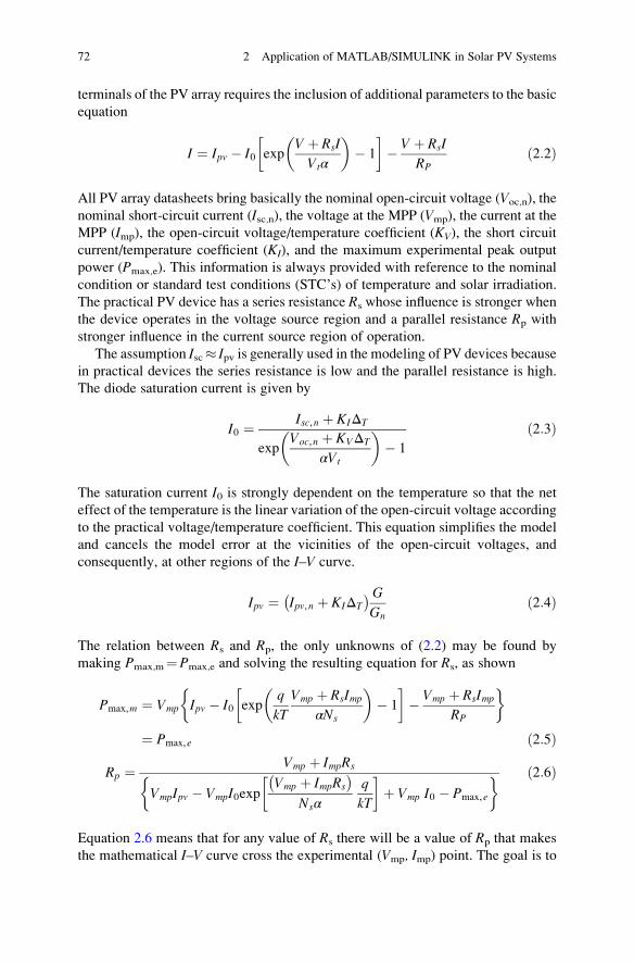
terminals of the PV array requires the inclusion of additional parameters to the basic
equation
I ¼ Ipv � I0 expV þ RsI
Vtα
� �� 1
� �� V þ RsI
RPð2:2Þ
All PV array datasheets bring basically the nominal open-circuit voltage (Voc,n), the
nominal short-circuit current (Isc,n), the voltage at the MPP (Vmp), the current at the
MPP (Imp), the open-circuit voltage/temperature coefficient (KV), the short circuit
current/temperature coefficient (KI), and the maximum experimental peak output
power (Pmax,e). This information is always provided with reference to the nominal
condition or standard test conditions (STC’s) of temperature and solar irradiation.
The practical PV device has a series resistance Rs whose influence is stronger when
the device operates in the voltage source region and a parallel resistance Rp with
stronger influence in the current source region of operation.
The assumption Isc� Ipv is generally used in the modeling of PV devices because
in practical devices the series resistance is low and the parallel resistance is high.
The diode saturation current is given by
I0 ¼ Isc,n þ KIΔT
expVoc,n þ KVΔT
αVt
� �� 1
ð2:3Þ
The saturation current I0 is strongly dependent on the temperature so that the net
effect of the temperature is the linear variation of the open-circuit voltage according
to the practical voltage/temperature coefficient. This equation simplifies the model
and cancels the model error at the vicinities of the open-circuit voltages, and
consequently, at other regions of the I–V curve.
Ipv ¼ Ipv,n þ KIΔT
� �GGn
ð2:4Þ
The relation between Rs and Rp, the only unknowns of (2.2) may be found by
making Pmax,m¼Pmax,e and solving the resulting equation for Rs, as shown
Pmax,m ¼ Vmp Ipv � I0 expq
kT
Vmp þ RsImpαNs
� �� 1
� �� Vmp þ RsImp
RP
�
¼ Pmax,e ð2:5Þ
Rp ¼ Vmp þ ImpRs
VmpIpv � VmpI0expVmp þ ImpRs
� �Nsα
q
kT
� �þ Vmp I0 � Pmax,e
� ð2:6Þ
Equation 2.6 means that for any value of Rs there will be a value of Rp that makes
the mathematical I–V curve cross the experimental (Vmp, Imp) point. The goal is to
72 2 Application of MATLAB/SIMULINK in Solar PV Systems
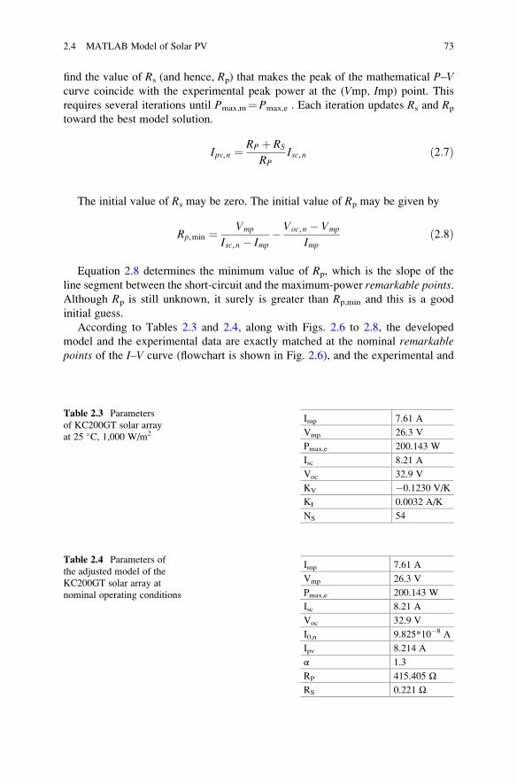
find the value of Rs (and hence, Rp) that makes the peak of the mathematical P–Vcurve coincide with the experimental peak power at the (Vmp, Imp) point. This
requires several iterations until Pmax,m¼Pmax,e . Each iteration updates Rs and Rp
toward the best model solution.
Ipv,n ¼ RP þ RS
RPIsc,n ð2:7Þ
The initial value of Rs may be zero. The initial value of Rp may be given by
Rp,min ¼ Vmp
Isc,n � Imp� Voc,n � Vmp
Impð2:8Þ
Equation 2.8 determines the minimum value of Rp, which is the slope of the
line segment between the short-circuit and the maximum-power remarkable points.Although Rp is still unknown, it surely is greater than Rp,min and this is a good
initial guess.
According to Tables 2.3 and 2.4, along with Figs. 2.6 to 2.8, the developed
model and the experimental data are exactly matched at the nominal remarkablepoints of the I–V curve (flowchart is shown in Fig. 2.6), and the experimental and
Table 2.3 Parameters
of KC200GT solar array
at 25 �C, 1,000 W/m2
Imp 7.61 A
Vmp 26.3 V
Pmax,e 200.143 W
Isc 8.21 A
Voc 32.9 V
KV �0.1230 V/K
KI 0.0032 A/K
NS 54
Table 2.4 Parameters of
the adjusted model of the
KC200GT solar array at
nominal operating conditions
Imp 7.61 A
Vmp 26.3 V
Pmax,e 200.143 W
Isc 8.21 A
Voc 32.9 V
I0,n 9.825*10�8 A
Ipv 8.214 A
α 1.3
RP 415.405 ΩRS 0.221 Ω
2.4 MATLAB Model of Solar PV 73
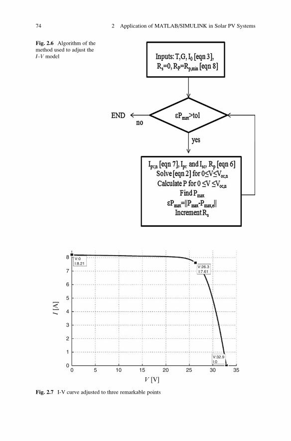
Fig. 2.6 Algorithm of the
method used to adjust the
I–V model
8
7
6
5
4
3
2
1
00 5 10 15 20 3025 35
V:26.3I:7.61
V:0I:8.21
V:32.9I:0
V [V]
I [A
]
Fig. 2.7 I-V curve adjusted to three remarkable points
74 2 Application of MATLAB/SIMULINK in Solar PV Systems
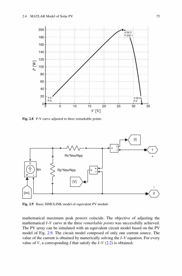
mathematical maximum peak powers coincide. The objective of adjusting the
mathematical I–V curve at the three remarkable points was successfully achieved.
The PV array can be simulated with an equivalent circuit model based on the PV
model of Fig. 2.9. The circuit model composed of only one current source. The
value of the current is obtained by numerically solving the I–V equation. For every
value of V, a corresponding I that satisfy the I–V (2.2) is obtained.
200
180
160
140
120
100
80
60
40
20
00 5 10 15 20 3025 35
V:26.3P:200.1
V:0P:0
V:32.9P:0
V [V]
P [W
]
Fig. 2.8 P-V curve adjusted to three remarkable points
Ipv
[Im]
[V]
[I]
1
2
–
+
+–i
Rp*Nss/Npp
Rs*Nss/Npp
s
+
+v
–
–
Fig. 2.9 Basic SIMULINK model of equivalent PV module
2.4 MATLAB Model of Solar PV 75

The model of the PV array was designed and the calculation of Im, Ipv and Io are
presented as separate sub-systems in Fig. 2.10.
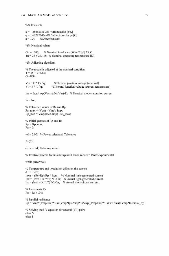
The parameters required for simulation are initialized by the following script file
Calculation of Im = Ipv-Id (Nss x Npp modules):
Calculation of lpv (single module):
Calculation of lo (single module):
[V]
[I]
[T]
[T]
Rs
XX eu
eu
X[Vta]
q/(a*k*Ns)
++
1
[Io]
+–
+
++
++
++
–
+–
+–
[Ipv]
X
[Im]
÷
÷Ki
Kv
Tn
X
X
÷X
X
X
[dT]
[dT]
Ipvn
[Ipv]
Gn
[G]
Vocn
[dT]
XX
[Vta]
1
Ki
Iscn [Io]
Fig. 2.10 SIMULINK model of the PV equations
76 2 Application of MATLAB/SIMULINK in Solar PV Systems
(continued)
2.4 MATLAB Model of Solar PV 77
(continued)
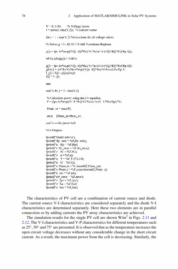
The characteristics of PV cell are a combination of current source and diode.
The current source V-I characteristics are considered separately and the diode V-I
characteristics are determined separately. Here these two elements are in parallel
connection so by adding currents the PV array characteristics are achieved.
The simulation results for the single PV cell are shown W/m2 in Figs. 2.11 and
2.12. The V-I characteristics and V-P characteristics for different temperatures such
as 25�, 50� and 75� are presented. It is observed that as the temperature increases the
open circuit voltage decreases without any considerable change in the short circuit
current. As a result, the maximum power from the cell is decreasing. Similarly, the
78 2 Application of MATLAB/SIMULINK in Solar PV Systems

V-I and V-P characteristics for radiations 500, 800, and 100 W/m2 are given.
For low values of solar radiations the short circuit current is reducing considerably
but the change in open circuit voltage is very less, thus proving that the maximum
power from the module is dropping.
2.4.1 SIMULINK Model of PV Module
This model contains an external control block permitting an uncomplicated varia-
tion of the models’ parameters. In this model, 36 PV cells are interconnected in
series to form one module. As a result, the module voltage is obtained by multi-
plying the cell voltage by the cells number while the total module current is the
same as the cell’s current.
4
3
2
1
00 5 10 V [Volts]
I [Amps] P [Watts]
1000 W/m2
800 W/m2
500 W/m2
1000 W/m2
800 W/m2
500 W/m2|
15 5 10 V [Volts] 15
5 100
80
60
40
20
00
Fig. 2.12 V-I and V-P characteristics to the variation in solar radiations
4
3
2
1
00 5 10 V [Volts]
25 deg
I [Amps] P [Watts]
50 deg 75 deg25 deg
50 deg
75 deg+
15 5 10 V [Volts] 15
5 100
80
60
40
20
00
Y A
xis
Y A
xis
Fig. 2.11 V-I and V-P characteristics to the variation in temperature
2.4 MATLAB Model of Solar PV 79
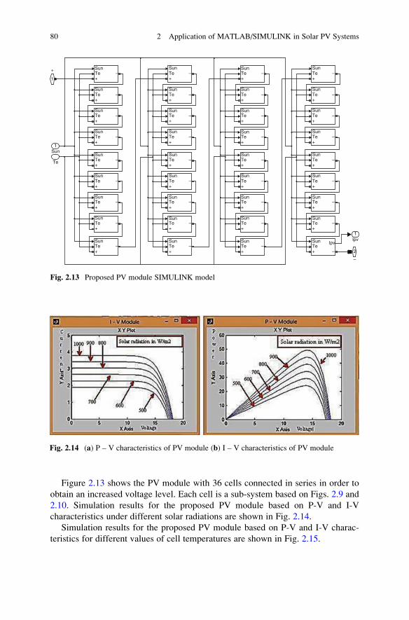
Figure 2.13 shows the PV module with 36 cells connected in series in order to
obtain an increased voltage level. Each cell is a sub-system based on Figs. 2.9 and
2.10. Simulation results for the proposed PV module based on P-V and I-V
characteristics under different solar radiations are shown in Fig. 2.14.
Simulation results for the proposed PV module based on P-V and I-V charac-
teristics for different values of cell temperatures are shown in Fig. 2.15.
SunTe+
–
SunTe+
–
SunTe+
–
SunTe+
–
SunTe+
–
SunTe+
–
SunTe+
–
SunTe+
–
SunTe+
–
SunTe+
–
SunTe+
–
SunTe+
–
SunTe+
–
SunTe+
–
SunTe+
–
SunTe+
–
SunTe+
–
SunTe+
–
SunTe+
–
SunTe+
–
SunTe+
–
SunTe+
–
SunTe+
–
SunTe+
–
SunTe+
–
SunTe+
–
SunTe+
–
SunTe+
–
SunTe+
–
SunTe+
–
SunTe+
–
SunTe+
–
SunTe+
–
SunTe+
–
SunTe+
–
SunTe+ –
–
1
2
lpvlpv
1Sun
Te
+
1
Fig. 2.13 Proposed PV module SIMULINK model
Fig. 2.14 (a) P – V characteristics of PV module (b) I – V characteristics of PV module
80 2 Application of MATLAB/SIMULINK in Solar PV Systems
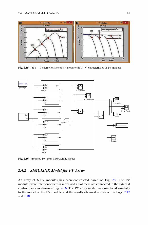
2.4.2 SIMULINK Model for PV Array
An array of 6 PV modules has been constructed based on Fig. 2.9. The PV
modules were interconnected in series and all of them are connected to the external
control block as shown in Fig. 2.16. The PV array model was simulated similarly
to the model of the PV module and the results obtained are shown in Figs. 2.17
and 2.18.
powergui
Continuous
Sun
Te
Sun
Te
+
Sun
Te
+
–
–
Sun
Te
+
–
Sun
Te
+
––
+
Sun
Te
+
–
Sun
Te
+
–
lpv
v
–
+v
X
X
I- V Module
P - V Module
I - V Panel
P - V Panel
Scope
Fig. 2.16 Proposed PV array SIMULINK model
Fig. 2.15 (a) P – V characteristics of PV module (b) I – V characteristics of PV module
2.4 MATLAB Model of Solar PV 81

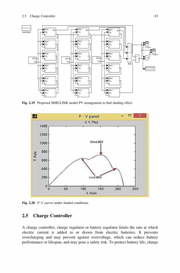
2.4.3 SIMULINK Model to Find Shading Effect
This section describes the procedure used for simulating the I–V and P–V charac-
teristics of a partially shaded PV array. It is important to understand how the
shading pattern and the PV array structure are defined in MATLAB (Fig. 2.19)
using the proposed scheme. The PV array is configured as a combination of six
series of PV modules connected in three parallel connections. Each set of PV
modules operate under different solar radiations and different cell temperatures.
The first set is under solar radiation of 800 W/m2 and cell temperature of 750 �C,second set is under solar radiation of 600 W/m2 and cell temperature of 250 �C, andthird set is under solar radiation of 700 W/m2 and cell temperature of 500 �C. Basedon these conditions the simulations illustrating the PV characteristics is shown in
Fig. 2.20 with three different multiple peaks. The maximum peak is called as global
peak and the remaining two peaks are called as the local peaks.
Fig. 2.17 (a) P – V characteristics of PV array (b) I – V characteristics of PV array
Fig. 2.18 (a) P – V characteristics for PV array (b) I – V characteristics for PV array
82 2 Application of MATLAB/SIMULINK in Solar PV Systems
2.5 Charge Controller
A charge controller, charge regulator or battery regulator limits the rate at which
electric current is added to or drawn from electric batteries. It prevents
overcharging and may prevent against overvoltage, which can reduce battery
performance or lifespan, and may pose a safety risk. To protect battery life, charge
Fig. 2.20 P–V curves under shaded conditions
Continuous
powergui
Sun
Sun
Te
Te+ –
lpv SunTe+ –
lpv
SunTe+
–SunTe+
–
SunTe+ –
lpv
SunTe+ +
+
++
v x
–
SunTe+
–
–
SunTe+
–
SunTe+
–
SunTe+
–
SunTe+
–
SunTe+
–
SunTe+
–
SunTe+
–
Sun
SunTe
Te
Sun
Te+
–
SunTe+
–
SunTe+
–
SunTe+
–
P - V panel
I - V panel
Add
Fig. 2.19 Proposed SIMULINK model PV arrangement to find shading effect
2.5 Charge Controller 83

controller may prevent battery from deep discharging or it will perform controlled
discharges, depending on the battery technology. The terms “charge controller” or
“charge regulator” may refer to either a stand-alone device, or to control circuitry
integrated within a battery pack, battery-powered device, or battery recharger.
Solar Charge Controllers are the controllers which regulate the power output or the
DC output voltage of the solar PV panels to the batteries. Charge controllers take the
DC output voltage as the input voltage converts it into same DC voltage required for
battery charging. These are mostly used in off grid scenario and uses Maximum
Power Point Tracking scheme which maximizes the output efficiency of the Solar PV
Panel. In battery charging system, the output voltage regulation is an important factor
as batteries require specific charging method with various voltage and current levels
for specific stage. These charging processes enhance battery performance and battery
life. Standard Charge controllers are used where the solar panel voltage used as input
are higher than the output voltage. Thus keeping the current constant, the voltage will
be reduced by the controller but it results in loss of power. MPPT based solar charge
controllers use microcontrollers based techniques to compute highest possible power
output at any given time i.e. voltage will be monitored and regulated without power
loss. The Controller will lower the voltage simultaneously increase the current,
thereby increasing the power transfer efficiency. To know much about the charge
controller, it is better to discuss about the batteries used in the PV system.
2.5.1 Batteries in PV Systems
Selecting the suitable battery for a PV application depends on many factors.
Specific decisions on battery selection depend on physical properties, while other
decisions will be much more difficult and may involve making tradeoffs between
desirable and undesirable battery features. With the proper application of this
knowledge, designers should be able to differentiate among battery types and
gain some application experience with batteries they are familiar with. Consider-
ations in battery subsystem design include the number of batteries is series and
parallel, over-current and disconnect requirements, and selection of the proper wire
sizes and types.
The energy output from the Solar PV systems is generally stored in a battery or in
a battery bank deepening upon the requirements of the system. Mostly batteries or
used in the stand-alone system and in the case of grid connected system, batteries are
used as a backup system. The primary functions of the battery in a PV system are:
(a) Energy Storage Capability and Autonomy: to store electrical energy when
it is produced by the PV array and to supply energy to electrical loads as
needed or on demand.
(b) Voltage and Current Stabilization: to supply power to electrical loads at
stable voltages and currents, by suppressing or ‘smoothing out’ transients thatmay occur in PV systems.
(c) Supply Surge Currents: to supply surge or high peak operating currents to
electrical loads or appliances.
84 2 Application of MATLAB/SIMULINK in Solar PV Systems
2.5.2 Battery Types and Classifications
Even batteries from the same manufactures differ in their performance and its
characteristics. Different manufacturers have variations in the details of their
battery construction, but some common construction features can be described for
almost all batteries. Batteries are generally mass produced; it consists of several
sequential and parallel processes to construct a complete battery unit. The
manufacturing is an intensive, heavy industrial process involving the use of haz-
ardous and toxic materials. After production, initial charge and discharge cycles are
conducted on batteries before they are shipped to distributors and consumers.
Different types of batteries are manufactured today, each with specific design for
particular applications. Each battery type or design has its individual strengths and
weaknesses. In solar PV system predominantly, lead-acid batteries are used due to
their wide availability in many sizes, low cost and well determined performance
characteristics. For low temperature applications nickel-cadmium cells are used, but
their high initial cost limits their use in most PV systems. The selection of the suitable
battery depends upon the application and the designer. In general, electrical storage
batteries can be divided into two major categories, primary and secondary batteries.
2.5.2.1 Primary Batteries
Primary batteries are non rechargeable but they can store and deliver electrical
energy. Typical carbon-zinc and lithium batteries commonly used primary batte-
ries. Primary batteries are not used in PV systems because they cannot be
recharged.
2.5.2.2 Secondary Batteries
Secondary batteries are rechargeable and they can store and deliver electrical
energy. Common lead-acid batteries used in automobiles and PV systems are
secondary batteries.
The batteries can be selected based on their design and performance character-
istics. The PV designer should consider the advantages and disadvantages of the
batteries based on its characteristics and with respect to the requirements of a
particular application. Some of the important parameters to be considered for the
selection of battery are lifetime, deep cycle performance, tolerance to high temper-
atures and overcharge, maintenance and many others.
2.5.3 Battery Charging
In a stand-alone PV system, the ways in which a battery is charged are generally
much different from the charging methods battery manufacturers use to rate battery
2.5 Charge Controller 85
performance. The battery charging in PV systems consists of three modes of battery
charging; normal or bulk charge, finishing or float charge and equalizing charge.
Bulk or Normal Charge: It is the initial portion of a charging cycle performed at
any charge rate and it occurs between 80 % and 90 % state of charge. This will
not allow the cell voltage to exceed the gassing voltage.
Float or Finishing Charge: It is usually conducted at low to medium charge rates.When the battery is fully charged, most of the active material in the battery has
been converted to its original form, generally voltage/current regulation are
required to limit the overcharge supplied to the battery.
Equalizing Charge: It consists of a current-limited charge to higher voltage limits
than set for the finishing or float charge. It is done periodically to maintain
consistency among individual cells. An equalizing charge is typically maintained
until the cell voltages and specific gravities remain consistent for a few hours.
2.5.4 Battery Discharging
Depth of Discharge (DOD): The battery DOD is defined as the percentage of
capacity that has been withdrawn from a battery compared to the total fully
charged capacity. The two common qualifiers for depth of discharge in PV
systems are the allowable or maximum DOD and the average daily DOD and
are described as follows:
Allowable DOD: The maximum percentage of full-rated capacity that can be
withdrawn from a battery is known as its allowable depth of discharge. The
allowable DOD is the maximum discharge limit for a battery, generally dictated
by the cut off voltage and discharge rate. In standalone PV systems, the lowvoltage load disconnect (LVD) set point of the battery charge controller dictatesthe allowable DOD limit at a given discharge rate.
Depending on the type of battery used in a PV system, the design allowable
depth of discharge may be as high as 80 % for deep cycle, motive power
batteries, to as low as 15–25 %. The allowable DOD is related to the autonomy,in terms of the capacity required to operate the system loads for a given number
of days without energy from the PV array.
Average Daily DOD: The average daily depth of discharge is the percentage of the
full-rated capacity that is withdrawn from a battery with the average daily loadprofile. If the load varies seasonally, the average daily DOD will be greater in the
winter months due to the longer nightly load operation period. For PV systems
with a constant daily load, the average daily DOD is generally greater in the
winter due to lower battery temperature and lower rated capacity. Depending on
the rated capacity and the average daily load energy, the average daily DOD
may vary between only a few percent in systems designed with a lot of auton-
omy, or as high as 50 % for marginally sized battery systems. The average daily
DOD is inversely related to autonomy; meaning that systems designed for longer
autonomy periods (more capacity) have a lower average daily DOD.
86 2 Application of MATLAB/SIMULINK in Solar PV Systems
State of Charge (SOC): The state of charge (SOC) is defined as the amount of energy
as a percentage of the energy stored in a fully charged battery. Discharging a
battery results in a decrease in state of charge, while charging results in an increase
in state of charge. A battery that has had three quarters of its capacity removed, or
been discharged 75 %, is said to be at 25 % state of charge.
Autonomy: Generally autonomy refers to the time a fully charged battery can
supply energy to the systems loads when there is no energy supplied by the
PV array. Longer autonomy periods generally result in a lower average daily
DOD and lower the probability that the allowable (maximum) DOD or minimum
load voltage is reached.
Self-Discharge Rate: In open-circuit mode without any charge or discharge current,
a battery undergoes a reduction in state of charge, due to internal mechanisms
and losses within the battery. Different battery types have different self-
discharge rates, the most significant factor being the active materials and grid
alloying elements used in the design.
Battery Lifetime: Battery lifetime is dependent upon a number of design and
operational factors, including the components and materials of battery construc-
tion, temperature, frequency, depth of discharges, and average state of charge
and charging methods.
Temperature Effects: For an electrochemical cell such as a battery, temperature has
important effects on performance. As the temperature increases by 10 �C, therate of an electrochemical reaction doubles, resulting in statements from battery
manufacturers that battery life decreases by a factor of two for every 10 �Cincrease in average operating temperature. Higher operating temperatures
accelerate corrosion of the positive plate grids, resulting in greater gassing and
electrolyte loss. Lower operating temperatures generally increase battery life.
However, the capacity is reduced significantly at lower temperatures, particu-
larly for lead-acid batteries. When severe temperature variations from room
temperatures exist, batteries are located in an insulated or other temperature-
regulated enclosure to minimize battery.
Effects of Discharge Rates: The higher the discharge rate or current, the lower the
capacity that can bewithdrawn from a battery to a specific allowableDODor cut off
voltage. Higher discharge rates also result in the voltage under load to be lower than
with lower discharge rates, sometimes affecting the selection of the low voltage
load disconnects set point. At the same battery voltage the lower the discharge rates,
the lower the battery state of charge compared to higher discharge rates.
Corrosion: The electrochemical activity resulting from the immersion of two
dissimilar metals in an electrolyte, or the direct contact of two dissimilar metals
causing one material to undergo oxidation or lose electrons and causing the
other material to undergo reduction, or gain electrons. Corrosion of the grids
supporting the active material in a battery is an ongoing process and may
ultimately dictate the battery’s useful lifetime. Battery terminals may also
experience corrosion due to the action of electrolyte gassing from the battery,
and generally require periodic cleaning and tightening in flooded lead-acid
types. Higher temperatures and the flow of electrical current between two
dissimilar metals accelerate the corrosion process.
2.5 Charge Controller 87

2.5.5 Battery Gassing and Overcharge Reaction
When the battery is nearly fully charged gassing occurs in a battery during
charging. At this point, essentially all of the active materials have been converted
to their fully charged composition and the cell voltage rises sharply. The gas
products are either recombined internal to the cell as in sealed or valve regulated
batteries, or released through the cell vents in flooded batteries. In battery, the
overcharge or gassing reaction is irreversible and it results in water loss. All gassing
reactions consume a portion of the charge current which cannot be delivered on the
subsequent discharge, thereby reducing the battery charging efficiency.
2.5.6 Charge Controller Types
There are two basic charge controller (i) Shunt Controller and (ii) Series Controller
2.5.6.1 Shunt Controller
Shunt controllers consists of a blocking diode in series between the battery and the
shunt element to prevent the battery from short-circuiting when the module is
regulating. This type of charge controllers are limited to use in Solar PV systems
with PV module currents less than 20 A. Shunt controller require a heat sink to
dissipate the power because of the voltage drop between the module and controller
and due to wiring and resistance of the shunt element, the module is never
entirely short circuited, resulting in some power dissipation within the controller.
Figure 2.21 below shows the diagram of shunt controller.
Fig. 2.21 Diagram of shunt controller
88 2 Application of MATLAB/SIMULINK in Solar PV Systems
2.5.6.2 Shunt-Interrupting Design
The shunt-interrupting controller completely disconnects the array current in an
interrupting or on-off fashion when the battery reaches the voltage regulation set
point. When the battery decreases to the array reconnect voltage, the controller
connects the array to resume charging the battery. This cycling between the
regulation voltage and array reconnect voltage is why these controllers are often
called on-off or pulsing controllers. Shunt-interrupting controllers are widely avail-
able and are low cost, however they are generally limited to use in systems with
array currents less than 20 A due to heat dissipation requirements. In general, on-off
shunt controllers consume less power than series type controllers that use relays, so
they are best suited for small systems where even minor parasitic losses become a
significant part of the system load. Shunt-interrupting charge controllers can be
used on all battery types; however the way in which they apply power to the battery
may not be optimal for all battery designs. In general, constant-voltage, PWM or
linear controller designs are recommended by manufacturers of gelled and AGM
lead-acid batteries. However, shunt-interrupting controllers are simple, low cost
and perform well in most small stand-alone PV systems.
2.5.6.3 Shunt-Linear Design
Once a battery becomes nearly fully charged, a shunt-linear controller maintains the
battery at near a fixed voltage by gradually shunting the array through a semicon-
ductor regulation element. In some designs, a comparator circuit in the controller
senses the battery voltage, and makes corresponding adjustments to the impedance
of the shunt element, thus regulating the array current. In other designs, simple
Zener power diodes are used, which are the limiting factor in the cost and power
ratings for these controllers. There is generally more heat dissipation in a shunt-
linear controller than in shunt-interrupting types. Shunt-linear controllers are
popular for use with sealed VRLA batteries. This algorithm applies power to the
battery in a preferential method for these types of batteries, by limiting the current
while holding the battery at the regulation voltage.
2.5.6.4 Series Controller
In a series controller, a relay or solid-state switch either opens the circuit between
the module and the battery to discontinuing charging, or limits the current in a
series-linear manner to hold the battery voltage at a high value. In the simpler series
interrupting design, the controller reconnects the module to the battery once
the battery falls to the module reconnect voltage set point. Figure 2.22 shows the
diagram of series controller.
2.5 Charge Controller 89

2.5.6.5 Series-Interrupting Design
The most simple series controller is the series-interrupting type, involving a
one-step control, turning the array charging current either on or off. The charge
controller constantly monitors battery voltage, and disconnects or open-circuits
the array in series once the battery reaches the regulation voltage set point.
After a pre-set period of time, or when battery voltage drops to the array
reconnect voltage set point, the array and battery are reconnected, and the cycle
repeats. As the battery becomes more fully charged, the time for the battery voltage
to reach the regulation voltage becomes shorter each cycle, so the amount of array
current passed through to the battery becomes less each time. In this way, full charge
is approached gradually in small steps or pulses, similar in operation to the shunt-
interrupting type controller. The principle difference is the series or shunt mode by
which the array is regulated. Similar to the shunt-interrupting type controller, the
series-interrupting type designs are best suited for use with flooded batteries rather
than the sealed VRLA types due to the way power is applied to the battery.
2.5.6.6 Series-Interrupting, 2-Step, Constant-Current Design
This type of controller is similar to the series-interrupting type, however when the
voltage regulation set point is reached, instead of totally interrupting the array
current, a limited constant current remains applied to the battery. This “trickle
charging” continues either for a pre-set period of time, or until the voltage drops to
the array reconnect voltage due to load demand. Then full array current is once
again allowed to flow, and the cycle repeats. Full charge is approached in a
continuous fashion, instead of smaller steps as described above for the on-off
type controllers. A load pulls down some two-stage controls increase array current
immediately as battery voltage. Others keep the current at the small trickle charge
level until the battery voltage has been pulled down below some intermediate value
(usually 12.5–12.8 V) before they allow full array current to resume.
Fig. 2.22 Diagram of series controller
90 2 Application of MATLAB/SIMULINK in Solar PV Systems
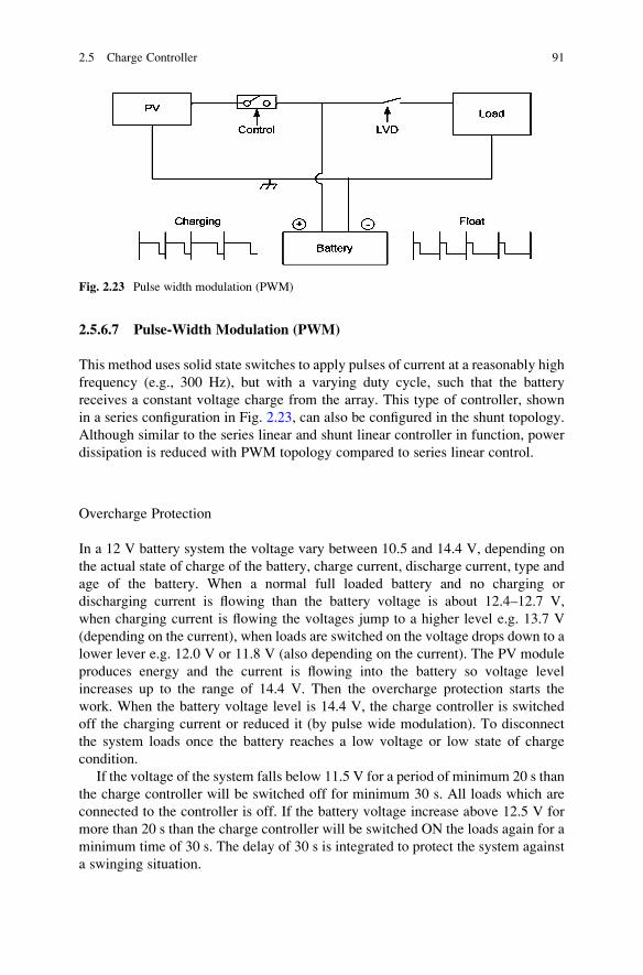
2.5.6.7 Pulse-Width Modulation (PWM)
This method uses solid state switches to apply pulses of current at a reasonably high
frequency (e.g., 300 Hz), but with a varying duty cycle, such that the battery
receives a constant voltage charge from the array. This type of controller, shown
in a series configuration in Fig. 2.23, can also be configured in the shunt topology.
Although similar to the series linear and shunt linear controller in function, power
dissipation is reduced with PWM topology compared to series linear control.
Overcharge Protection
In a 12 V battery system the voltage vary between 10.5 and 14.4 V, depending on
the actual state of charge of the battery, charge current, discharge current, type and
age of the battery. When a normal full loaded battery and no charging or
discharging current is flowing than the battery voltage is about 12.4–12.7 V,
when charging current is flowing the voltages jump to a higher level e.g. 13.7 V
(depending on the current), when loads are switched on the voltage drops down to a
lower lever e.g. 12.0 V or 11.8 V (also depending on the current). The PV module
produces energy and the current is flowing into the battery so voltage level
increases up to the range of 14.4 V. Then the overcharge protection starts the
work. When the battery voltage level is 14.4 V, the charge controller is switched
off the charging current or reduced it (by pulse wide modulation). To disconnect
the system loads once the battery reaches a low voltage or low state of charge
condition.
If the voltage of the system falls below 11.5 V for a period of minimum 20 s than
the charge controller will be switched off for minimum 30 s. All loads which are
connected to the controller is off. If the battery voltage increase above 12.5 V for
more than 20 s than the charge controller will be switched ON the loads again for a
minimum time of 30 s. The delay of 30 s is integrated to protect the system against
a swinging situation.
Fig. 2.23 Pulse width modulation (PWM)
2.5 Charge Controller 91
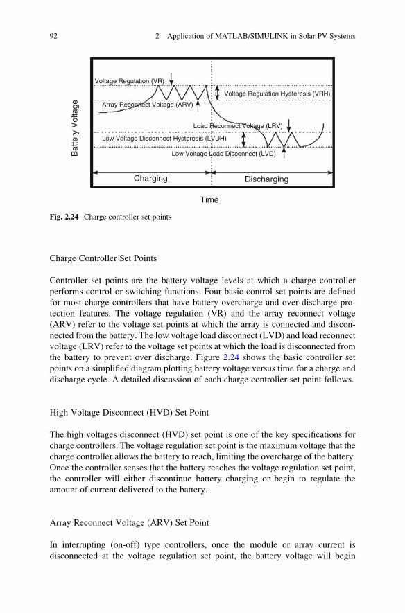
Charge Controller Set Points
Controller set points are the battery voltage levels at which a charge controller
performs control or switching functions. Four basic control set points are defined
for most charge controllers that have battery overcharge and over-discharge pro-
tection features. The voltage regulation (VR) and the array reconnect voltage
(ARV) refer to the voltage set points at which the array is connected and discon-
nected from the battery. The low voltage load disconnect (LVD) and load reconnect
voltage (LRV) refer to the voltage set points at which the load is disconnected from
the battery to prevent over discharge. Figure 2.24 shows the basic controller set
points on a simplified diagram plotting battery voltage versus time for a charge and
discharge cycle. A detailed discussion of each charge controller set point follows.
High Voltage Disconnect (HVD) Set Point
The high voltages disconnect (HVD) set point is one of the key specifications for
charge controllers. The voltage regulation set point is the maximum voltage that the
charge controller allows the battery to reach, limiting the overcharge of the battery.
Once the controller senses that the battery reaches the voltage regulation set point,
the controller will either discontinue battery charging or begin to regulate the
amount of current delivered to the battery.
Array Reconnect Voltage (ARV) Set Point
In interrupting (on-off) type controllers, once the module or array current is
disconnected at the voltage regulation set point, the battery voltage will begin
Low Voltage Disconnect Hysteresis (LVDH)
Low Voltage Load Disconnect (LVD)
Voltage Regulation (VR)
Voltage Regulation Hysteresis (VRH)
Array Reconnect Voltage (ARV)
Load Reconnect Voltage (LRV)
Charging Discharging
Time
Bat
tery
Vol
tage
Fig. 2.24 Charge controller set points
92 2 Application of MATLAB/SIMULINK in Solar PV Systems
to decrease. If the charge and discharge rates are high, the battery voltage will
decrease at a greater rate when the battery voltage decreases to a predefined voltage,
the module is again reconnected to the battery for charging. The voltage at
which the module is reconnected is defined as the array reconnects voltage
(ARV) set point.
Deep Discharge Protection
When a battery is deeply discharged, the reaction in the battery occurs close to the
grids, and weakens the bond between the active materials and the grids. When we
deep discharge the battery repeatedly, loss of capacity and life will eventually
occur. To protect battery from deep discharge, most charge controllers include an
optional feature.
2.5.6.8 Voltage Regulation Hysteresis (VRH)
The voltage differences between the high voltages disconnect set point and
the array reconnect voltage is often called the voltage regulation hysteresis
(VRH). The VRH is a major factor which determines the effectiveness of battery
recharging for interrupting (on-off) type controller. If the hysteresis is too big, the
module current remains disconnected for long periods, effectively lowering
the module energy utilization and making it very difficult to fully recharge the
battery. If the regulation hysteresis is too small, the module will cycle on and off
rapidly. Most interrupting (on-off) type controllers have hysteresis values between
0.4 and 1.4 V for nominal 12 V systems.
2.5.6.9 Low Voltage Load Disconnect (LVD) Set Point
Deep discharging the battery can make it susceptible to freezing and shorten its
operating life. If battery voltage drops too low, due to prolonged bad weather or
certain non-essential loads are connected the charge controller disconnected the
load from the battery to prevent further discharge. This can be done using a low
voltage load disconnect (LVD) device is connected between the battery and
non-essential loads. The LVD is either a relay or a solid-state switch that interrupts
the current from the battery to the load.
2.5.6.10 Load Reconnect Voltage (LRV) Set Point
The battery voltage at which a controller allows the load to be reconnected to the
battery is called the load reconnect voltage (LRV). After the controller disconnects
the load from the battery at the LVD set point, the battery voltage rises to its
2.5 Charge Controller 93
open-circuit voltage. When the PV module connected for charging, the battery
voltage rises even more. At some point, the controller senses that the battery voltage
and state of charge are high enough to reconnect the load, called the load reconnect
voltage set point. LRV should be 0.08 V/cell (or 0.5 V per 12 V) higher than the
load-disconnection voltage. Typically LVD set points used in small PV systems are
between 12.5 and 13.0 V for most nominal 12 V lead-acid battery. If the LRV set
point is selected too low, the load may be reconnected before the battery has been
charged.
2.5.6.11 Low Voltage Load Disconnect Hysteresis (LVLH)
The voltage difference between the low voltage disconnect set point and the load
reconnect voltage is called the low voltage disconnect hysteresis. If the low voltage
disconnect hysteresis is too small, the load may cycle on and off rapidly at low
battery state-of-charge (SOC), possibly damaging the load or controller, and
extending the time it required to charge the battery fully. If the low voltage
disconnect hysteresis is too large the load may remain off for extended periods
until the array fully recharges the battery.
2.5.7 Charge Controller Selection
Charge controllers are used in Solar PV systems to allow high rates of charging
up to the gassing point, and then limit or disconnect the PV current to prevent
overcharge. The highest voltage that batteries are allowed to reach depends on how
much gassing occurs. To limit gassing, proper selection of the charge controller
voltage regulation set point is critical in PV systems. Both under and overcharging
will result in premature battery failure and loss of load in stand-alone PV systems.
The selection and sizing of charge controllers in PV systems involves the consid-
eration of several factors, depending on the complexity and control options
required. While the primary function is to prevent battery overcharge, many other
functions may also be used, including low voltage load disconnect, load regulation
and control, control of backup energy sources, diversion of energy to and auxiliary
load, and system monitoring. The designer must decide which options are needed to
satisfy the requirements of a specific application.
The charge controller must not only be able to handle typical or rated voltages
and currents, but must also be sized to handle expected peak or surge conditions
from the PV array or required by the electrical loads that may be connected to the
controller. It is extremely important that the controller be adequately sized for the
intended application. The sizing of the charge controller can be determined by
multiplying the short-circuit current of the solar PV module and the safety factor.
94 2 Application of MATLAB/SIMULINK in Solar PV Systems
2.5.8 Operating Without a Charge Controller
Charge controller is an essential part in stand-alone PV systems. However there
are special circumstances where a charge controller may not be needed in small
systems with well-defined loads. By eliminating the need for the sensitive elec-
tronic charge controller, the design is simplified, at lower cost and with improved
reliability. There are two cases where battery charge regulation may not be
required: (1) when a low voltage “self-regulating module” is used in the proper
climate; and (2) when the battery is very large compared to the array. Each of these
cases are discussed next.
2.5.9 Using Low-Voltage “Self-Regulating” Modules
A Self-regulating system consists of a low voltage solar PV module, battery and
load. Solar PV module is used to charge a 12 V battery. In the case self-regulating
modules without battery charge regulation, the array current falls off sharply as
the voltage increases above the maximum power point. In a “self-regulating” low
voltage PV module, there are generally only 28–30 silicon cells connected in series,
resulting in an open-circuit voltage of about 18 V and a maximum power voltage of
about 15 V at 25 �C. For every 1 �C increase in temperature, module voltage
decreases by 2.3 mV. For self-regulation and no battery overcharge to occur, the
following three conditions must be met:
1. The load must be used daily. Every day the battery will receive excessive
charge, even if the module is forced to operate beyond the “knee” at current
levels lower than its Imp. If the load is used daily, then the amp-hours produced
by the module are removed from the battery, and this energy can be safely
replaced the next day without overcharging the battery. So for a system to be
“self-regulating”, the load must be consistent and predictable.
2. The climate cannot be too cold. If the module stays very cool, the “knee” of the
IV curve will not move down in voltage enough, and the expected drop off
in current will not occur, even if the battery voltage rises as expected.
Often “self-regulating modules” are used in arctic climates for lighting for
remote cabins for example, because they are the smallest and therefore least
expensive of the power modules, but they are combined with a charge controller
or voltage dropping diodes to prevent battery overcharge.
3. The climate cannot be too warm. If the module heats up too much, then the drop
off in current will be too extreme, and the battery may never be properly
recharged. The battery will sulfate, and the loads will not be able to operate.
A “self-regulating system” design can greatly simplify the design by eliminating
the need for a charge controller, however these type of designs are only appro-
priate for certain applications and conditions. In most common stand-alone PV
system designs, a battery charge controller is required.
2.5 Charge Controller 95

2.5.10 Using a Large Battery or Small Array
A charge controller may not be needed if the charge rates delivered by the array to the
battery are small enough to prevent the battery voltage from exceeding the gassing
voltage limit when the battery is fully charged and the full array current is applied. In
certain applications, a long autonomy period may be used, resulting in a large amount
of battery storage capacity. In these cases, the charge rates from the array may be very
low, and can be accepted by the battery at any time without overcharging. These
situations are common in critical application requiring large battery storage, such as
telecommunications repeaters in alpine conditions or remote navigational aids. It
might also be the case when a very small load and array are combined with a large
battery, as in remote telemetry systems. In general a charging rate of C/100 or less is
considered low enough to be tolerated for long periods even when the battery is fully
charged. This means that even during the peak of the day, the array is charging the
battery bank at the 100 h rate or slower, equivalent to the typical trickle charge rate
that a controller would produce anyway.
2.6 MATLAB Model of SOC
The implementation of State of charge battery using MATLAB/SIMULINK is
presented in this section. This simulation focuses on knowing the state of charge
of a battery by connecting it to a load with constant charging and discharging.
Assumptions
• The internal resistance is maintained constant during the charge and the
discharge cycles and does not vary with the amplitude of the current.
• The parameters of the model are deduced from discharge characteristics and
assumed to be the same for charging.
• The capacity of the battery doesn’t change with the amplitude of current
(No Peukert effect).
• The model doesn’t take the temperature into account.
• The Self-Discharge of the battery is not represented. It can be represented by
adding a large resistance in parallel with the battery terminals.
• The battery has no memory effect.
Limitations
Theminimum no-load battery voltage is 0 V and themaximum battery voltage is equal
to 2*E0. The minimum capacity of the battery is 0 Ah and the maximum capacity is
Qmax. The equivalent circuit of a generic dynamic battery model parameterized to
represent most popular types of rechargeable batteries is shown in Fig. 2.25.
In this section, Nickel-Cadmium and Nickel-Metal-Hydride model is
implemented using SIMULINK. The corresponding equations for charge and
discharge model are represented according to the following equations.
96 2 Application of MATLAB/SIMULINK in Solar PV Systems
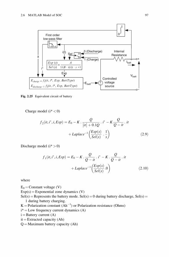
Charge model (i*< 0)
f 2 it, i�, i,Expð Þ ¼ E0 � K :Qitþ 0:1Q
: i� � K:Q
Q� it: it
þ Laplace�1 Exp sð ÞSel sð Þ :
1
s
� �ð2:9Þ
Discharge model (i*> 0)
f 1 it, i�, i,Expð Þ ¼ E0 � K :Q
Q� it: i� � K :
Q
Q� it: it
þ Laplace�1 Exp sð ÞSel sð Þ :0
� �ð2:10Þ
where
E0¼Constant voltage (V)
Exp(s)¼Exponential zone dynamics (V)
Sel(s)¼Represents the battery mode. Sel(s)¼ 0 during battery discharge, Sel(s)¼1 during battery charging.
K¼ Polarization constant (Ah�1) or Polarization resistance (Ohms)
i*¼Low frequency current dynamics (A)
i¼Battery current (A)
it¼Extracted capacity (Ah)
Q¼Maximum battery capacity (Ah)
Sel
=
First orderlow-pass filter
0 (Discharge)
1 (Charge)
Controlledvoltagesource
InternalResistance
Vbatt
Ebatt
Ibatt
it
i(t)
0
t
+
+
–
–
Exp
i*
Exp (s)
Edischarge = f2(it, i*, Exp, BattType)
Echarge = f1(it, i*, Exp, BattType)
A
Sel (s) 1/(B . i(t)) . s +1
Fig. 2.25 Equivalent circuit of battery
2.6 MATLAB Model of SOC 97
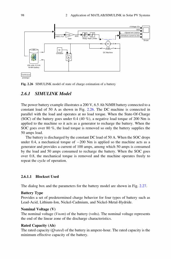
2.6.1 SIMULINK Model
The power battery example illustrates a 200 V, 6.5 Ah NiMH battery connected to a
constant load of 50 A as shown in Fig. 2.26. The DC machine is connected in
parallel with the load and operates at no load torque. When the State-Of-Charge
(SOC) of the battery goes under 0.4 (40 %), a negative load torque of 200 Nm is
applied to the machine so it acts as a generator to recharge the battery. When the
SOC goes over 80 %, the load torque is removed so only the battery supplies the
50 amps load.
The battery is discharged by the constant DC load of 50 A. When the SOC drops
under 0.4, a mechanical torque of �200 Nm is applied so the machine acts as a
generator and provides a current of 100 amps, among which 50 amps is consumed
by the load and 50 amps consumed to recharge the battery. When the SOC goes
over 0.8, the mechanical torque is removed and the machine operates freely to
repeat the cycle of operation.
2.6.1.1 Blockset Used
The dialog box and the parameters for the battery model are shown in Fig. 2.27.
Battery Type
Provides a set of predetermined charge behavior for four types of battery such as
Lead-Acid, Lithium-Ion, Nickel-Cadmium, and Nickel-Metal-Hydride.
Nominal Voltage (V)
The nominal voltage (Vnom) of the battery (volts). The nominal voltage represents
the end of the linear zone of the discharge characteristics.
Rated Capacity (Ah)
The rated capacity (Qrated) of the battery in ampere-hour. The rated capacity is the
minimum effective capacity of the battery.
Continuous
powergui
200 volts, 6.5 AhNi-MH battery
Constant
50+
–
GainSOC
Relay Rate Limiter
1/100<SOC (%)>
m
s
+
–
DC Machine
A+
F+
A–
F–
TL m
DC
<Voltage (V)>
<Speed wm (rad/s)>
<Armature current ia (A)>
SOC
Scope
Fig. 2.26 SIMULINK model of state of charge estimation of a battery
98 2 Application of MATLAB/SIMULINK in Solar PV Systems
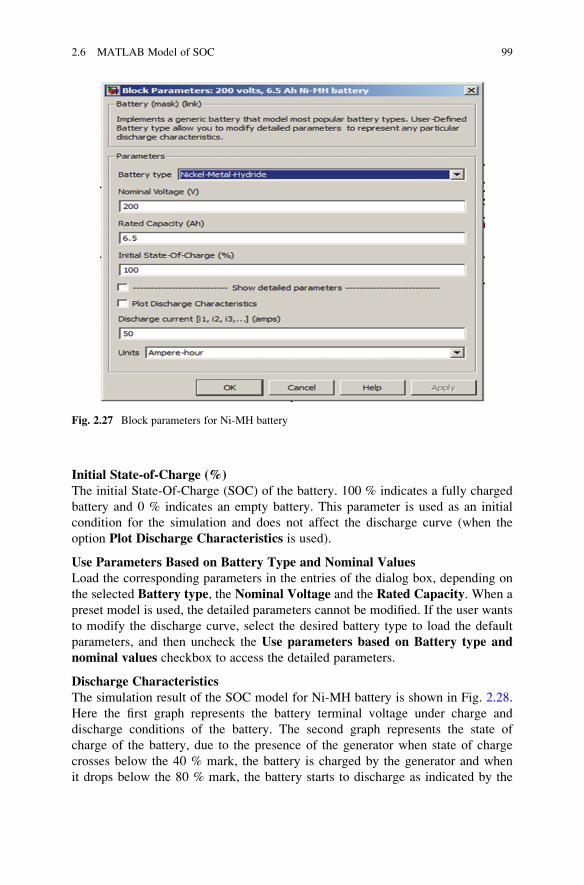
Initial State-of-Charge (%)
The initial State-Of-Charge (SOC) of the battery. 100 % indicates a fully charged
battery and 0 % indicates an empty battery. This parameter is used as an initial
condition for the simulation and does not affect the discharge curve (when the
option Plot Discharge Characteristics is used).
Use Parameters Based on Battery Type and Nominal ValuesLoad the corresponding parameters in the entries of the dialog box, depending on
the selected Battery type, the Nominal Voltage and the Rated Capacity. When a
preset model is used, the detailed parameters cannot be modified. If the user wants
to modify the discharge curve, select the desired battery type to load the default
parameters, and then uncheck the Use parameters based on Battery type and
nominal values checkbox to access the detailed parameters.
Discharge Characteristics
The simulation result of the SOC model for Ni-MH battery is shown in Fig. 2.28.
Here the first graph represents the battery terminal voltage under charge and
discharge conditions of the battery. The second graph represents the state of
charge of the battery, due to the presence of the generator when state of charge
crosses below the 40 % mark, the battery is charged by the generator and when
it drops below the 80 % mark, the battery starts to discharge as indicated by the
Fig. 2.27 Block parameters for Ni-MH battery
2.6 MATLAB Model of SOC 99
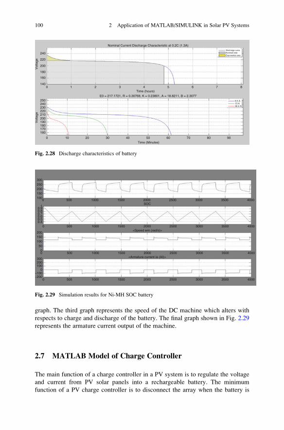
graph. The third graph represents the speed of the DC machine which alters with
respects to charge and discharge of the battery. The final graph shown in Fig. 2.29
represents the armature current output of the machine.
2.7 MATLAB Model of Charge Controller
The main function of a charge controller in a PV system is to regulate the voltage
and current from PV solar panels into a rechargeable battery. The minimum
function of a PV charge controller is to disconnect the array when the battery is
300
200250
150100
200
200
–200
300
150100
100
–100
500
0
10.90.80.70.60.50.4
0 500 1000 1500 2000SOC
<Speed wm (rad/s)>
<Armature current ia (AI)>
2500 3000 3500 4000
0 500 1000 1500 2000 2500 3000 3500 4000
0 500 1000 1500 2000 2500 3000 3500 4000
0 500 1000 1500 2000 2500 3000 3500 4000
Fig. 2.29 Simulation results for Ni-MH SOC battery
240
220
200
180
160
1400
0 10 20 30 40 50Time (Minutes)
60 70 80 90
1
Vol
tage
Vol
tage
2 3 4Time (hours)
Nominal Current Discharge Characteristic at 0.2C (1.3A)
E0 = 217.1721, R = 0.30769, K = 0.23801, A = 18.8211, B = 2.3077
5 6 7 8
250240230220210200190180170160
Discharge curve
6.5 A
32.5 A13 A
Exponential areaNominal area
Fig. 2.28 Discharge characteristics of battery
100 2 Application of MATLAB/SIMULINK in Solar PV Systems
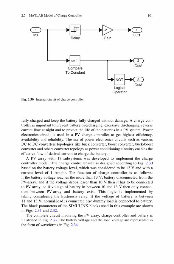
fully charged and keep the battery fully charged without damage. A charge con-
troller is important to prevent battery overcharging, excessive discharging, reverse
current flow at night and to protect the life of the batteries in a PV system. Power
electronics circuit is used in a PV charge-controller to get highest efficiency,
availability and reliability. The use of power electronics circuits such as various
DC to DC converters topologies like buck converter, boost converter, buck-boost
converter and others converter topology as power conditioning circuitry enables the
effective flow of desired current to charge the battery.
A PV array with 17 subsystems was developed to implement the charge
controller model. The charge controller unit is designed according to Fig. 2.30
based on the battery voltage level, which was considered to be 12 V and with a
current level of 1 Amphr. The function of charge controller is as follows:
if the battery voltage reaches the more than 13 V, battery disconnected from the
PV-array, and if the voltage drops lesser than 10 V then it has to be connected
to PV array, so if voltage of battery in between 10 and 13 V then only connec-
tion between PV-array and battery exist. This logic is implemented by
taking considering the hysteresis relay. If the voltage of battery is between
11 and 13 V, normal load is connected else dummy load is connected to battery.
The block parameters of the SIMULINK blocks used in this example are shown
in Figs. 2.31 and 2.32.
The complete circuit involving the PV array, charge controller and battery is
illustrated in Fig. 2.33. The battery voltage and the load voltage are represented in
the form of waveforms in Fig. 2.34.
1
In1Relay Gain
CompareTo Constant
LogicalOperator
Out1
Out2
Out3NOT 3
2
1-2
<= 11
Fig. 2.30 Internal circuit of charge controller
2.7 MATLAB Model of Charge Controller 101

Fig. 2.32 Block parameters of ideal switch
Fig. 2.31 Block parameters of Ni-MH battery
102 2 Application of MATLAB/SIMULINK in Solar PV Systems
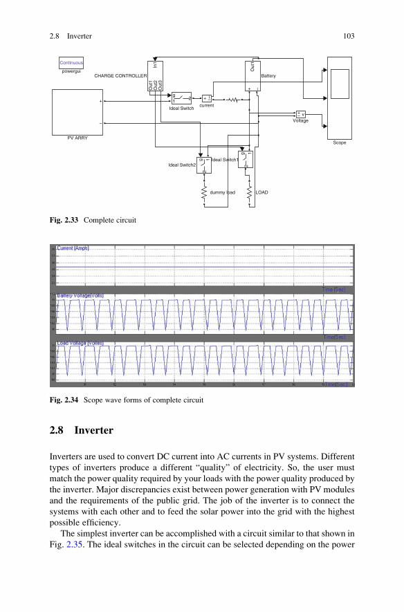
2.8 Inverter
Inverters are used to convert DC current into AC currents in PV systems. Different
types of inverters produce a different “quality” of electricity. So, the user must
match the power quality required by your loads with the power quality produced by
the inverter. Major discrepancies exist between power generation with PV modules
and the requirements of the public grid. The job of the inverter is to connect the
systems with each other and to feed the solar power into the grid with the highest
possible efficiency.
The simplest inverter can be accomplished with a circuit similar to that shown in
Fig. 2.35. The ideal switches in the circuit can be selected depending on the power
Fig. 2.34 Scope wave forms of complete circuit
Continuous
powergui
PV ARRY
+
–
CHARGE CONTROLLER
Ideal Switch
Ideal Switch2Ideal Switch1
current
g
g
g
1+2
1
1
2
2
i–
Out
1O
ut2
Out
3In
1
+
+
–
–
vVoltage
Battery
Out
1
Scope
LOADdummy load
Fig. 2.33 Complete circuit
2.8 Inverter 103
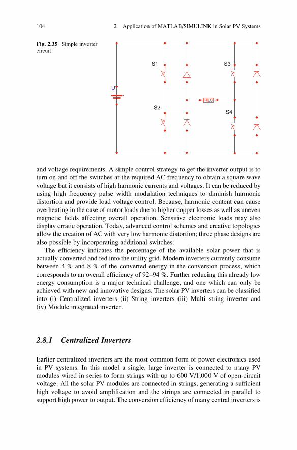
and voltage requirements. A simple control strategy to get the inverter output is to
turn on and off the switches at the required AC frequency to obtain a square wave
voltage but it consists of high harmonic currents and voltages. It can be reduced by
using high frequency pulse width modulation techniques to diminish harmonic
distortion and provide load voltage control. Because, harmonic content can cause
overheating in the case of motor loads due to higher copper losses as well as uneven
magnetic fields affecting overall operation. Sensitive electronic loads may also
display erratic operation. Today, advanced control schemes and creative topologies
allow the creation of AC with very low harmonic distortion; three phase designs are
also possible by incorporating additional switches.
The efficiency indicates the percentage of the available solar power that is
actually converted and fed into the utility grid. Modern inverters currently consume
between 4 % and 8 % of the converted energy in the conversion process, which
corresponds to an overall efficiency of 92–94 %. Further reducing this already low
energy consumption is a major technical challenge, and one which can only be
achieved with new and innovative designs. The solar PV inverters can be classified
into (i) Centralized inverters (ii) String inverters (iii) Multi string inverter and
(iv) Module integrated inverter.
2.8.1 Centralized Inverters
Earlier centralized inverters are the most common form of power electronics used
in PV systems. In this model a single, large inverter is connected to many PV
modules wired in series to form strings with up to 600 V/1,000 V of open-circuit
voltage. All the solar PV modules are connected in strings, generating a sufficient
high voltage to avoid amplification and the strings are connected in parallel to
support high power to output. The conversion efficiency of many central inverters is
RLC
S1 S3
S4S2
U
Fig. 2.35 Simple inverter
circuit
104 2 Application of MATLAB/SIMULINK in Solar PV Systems
95 % or higher, and they feature a relatively low unit cost per watt. However,
central inverters have multiple drawbacks.
This main disadvantage of this topology is the involvement of high voltage DC
cable from the strings to the inverter and losses in string diodes. This structure is
also limited from Maximum Power Point (MPP) Tracking and controlling
mismatch between strings so individual PVs, resulting in low efficiency and
reliability. This topology is not flexible and this makes it less appealing in mass
production. With all these issues, this technology is not used in new solar PV
systems installation. Central inverters (Fig. 2.36) cannot monitor the performance
of individual PVmodules, so damaged or otherwise compromised modules often go
undetected. Finally, central inverters limit the design and site selection of PV
systems, particularly in residential applications. They require co-planar module
layouts and a lack of partial shading from chimneys, trees, vent pipes, etc. PV
installers may opt out of half or more of potential sites due to these restrictions.
The conversion efficiency of many central inverters is 95 % or higher, and they
feature a relatively low unit cost per watt. Generally for high voltage PV systems
central inverters are preferred mainly because for systems ranging from 5 kW to
1 MW, incentives are provided by government agencies. Certain centralized
inverters uses common MPPT and IGBT based topology for enhancing power
quality. In some power plants, central inverters were arranged in master slave
configurations in order to use the most efficient combination of inverters according
to total PV array output. Presently central inverters can be installed along with
the DC-DC Optimizers. DC-DC optimizers supplement a central inverter with
individual DC-DC converters installed for each PV module (Fig. 2.37). DC-DC
optimizers can be wired serially in strings and also it can be wired in parallel.
The central inverter still converts the combined DC output from across the array to
grid-compatible AC power, but the DC-DC optimizers perform MPPT at the
module level. This allows each module to produce its full output without being
held back by any under-performing modules in the array. DC-DC optimizers also
permit module-level communications and performance monitoring. However,
DC-DC optimizers retain a key disadvantage of central inverters–a failure of the
central inverter still results in a complete loss of system output. Furthermore, some
DC-DC optimizer systems also require a separate command-and-control device to
operate, creating one more point of potential system failure in addition to the central
To Grid
PV Module PV Module
PV Module PV Module
Inverter
Fig. 2.36 Centralized inverters
2.8 Inverter 105
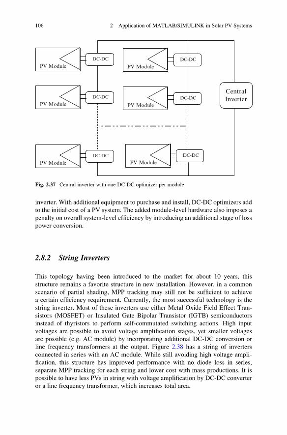
inverter. With additional equipment to purchase and install, DC-DC optimizers add
to the initial cost of a PV system. The added module-level hardware also imposes a
penalty on overall system-level efficiency by introducing an additional stage of loss
power conversion.
2.8.2 String Inverters
This topology having been introduced to the market for about 10 years, this
structure remains a favorite structure in new installation. However, in a common
scenario of partial shading, MPP tracking may still not be sufficient to achieve
a certain efficiency requirement. Currently, the most successful technology is the
string inverter. Most of these inverters use either Metal Oxide Field Effect Tran-
sistors (MOSFET) or Insulated Gate Bipolar Transistor (IGTB) semiconductors
instead of thyristors to perform self-commutated switching actions. High input
voltages are possible to avoid voltage amplification stages, yet smaller voltages
are possible (e.g. AC module) by incorporating additional DC-DC conversion or
line frequency transformers at the output. Figure 2.38 has a string of inverters
connected in series with an AC module. While still avoiding high voltage ampli-
fication, this structure has improved performance with no diode loss in series,
separate MPP tracking for each string and lower cost with mass productions. It is
possible to have less PVs in string with voltage amplification by DC-DC converter
or a line frequency transformer, which increases total area.
CentralInverter
PV ModuleDC-DC
PV ModuleDC-DC
PV ModuleDC-DC
PV ModuleDC-DC
PV ModuleDC-DC
PV ModuleDC-DC
Fig. 2.37 Central inverter with one DC-DC optimizer per module
106 2 Application of MATLAB/SIMULINK in Solar PV Systems

2.8.3 Multi-string Inverters
In this structure as shown in Fig. 2.39, DC-DC converter is implemented for
each string for MPP tracking and power combination of different string to a
DC bus. Multi-string inverter features the optimal MPP tracking for a single string
of PVs. A big power stage works as a grid connected half bridge inverter without
transformer. The multi-string inverter is useful when PV strings of different rated
power, different orientation are combined. The DC-DC part can be implemented
with high-frequency pulse width modulation (PWM) converter to reduce imple-
mentation area.
2.8.4 Module Integrated Inverter/Micro-inverters
Micro inverters (Fig. 2.40) are a complete, environmentally protected unit
consisting of solar cells, optics, inverter, and other components, designed to
generate AC power when exposed to sunlight. Module-level micro-inverters were
first introduced to the PV market in the 1990s but now they progressed to the point
and it became the alternative solution to the central inverters most commonly used
today in PV systems. It is predicted that within a few years most PV modules will
feature some form of module-level power electronics. The micro-inverter,
To Grid
CentralInverter
PV ModulePV Module
Inverter
PV Module
Inverter
PV Module
Control Unit
Fig. 2.39 Multi-string inverters
PV Module
Inverter
PV Module
Fig. 2.38 String inverters
2.8 Inverter 107
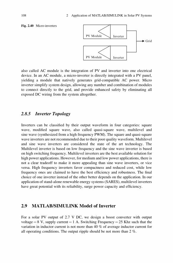
also called AC module is the integration of PV and inverter into one electrical
device. In an AC module, a micro-inverter is directly integrated with a PV panel,
yielding a module that natively generates grid-compatible AC power. Micro
inverter simplify system design, allowing any number and combination of modules
to connect directly to the grid, and provide enhanced safety by eliminating all
exposed DC wiring from the system altogether.
2.8.5 Inverter Topology
Inverters can be classified by their output waveform in four categories: square
wave, modified square wave, also called quasi-square wave, multilevel and
sine wave (synthesized from a high frequency PWM). The square and quasi-square
wave inverters are not recommended due to their poor quality waveform. Multilevel
and sine wave inverters are considered the state of the art technology. The
Multilevel inverter is based on low frequency and the sine wave inverter is based
on high switching frequency. Multilevel inverters are the best available solution for
high power applications. However, for medium and low power applications, there is
not a clear tradeoff to make it more appealing than sine wave inverters, or vice
versa. High frequency inverters favor compactness and reduced cost, while low
frequency ones are claimed to have the best efficiency and robustness. The final
choice of one inverter instead of the other better depends on the application. In our
application of stand-alone renewable energy systems (SARES), multilevel inverters
have great potential with its reliability, surge power capacity and efficiency.
2.9 MATLAB/SIMULINK Model of Inverter
For a solar PV output of 2.7 V DC, we design a boost converter with output
voltage¼ 8 V, supply current¼ 1 A. Switching Frequency¼ 25 Khz such that the
variation in inductor current is not more than 40 % of average inductor current for
all operating conditions. The output ripple should be not more than 2 %.
Grid
PV Module Inverter
PV Module Inverter
Fig. 2.40 Micro-inverters
108 2 Application of MATLAB/SIMULINK in Solar PV Systems

DC-DC Converter (Boost)
In a boost converter, the output voltage is related to input voltage by the formula
vo ¼ VIN
1� kð Þ
Switching frequency¼ 25 kHz
Vin¼ 2.7 V To obtain an output of 8 V and load current of 1 A,
8 ¼ 2:7
1� kð Þ K ¼ 0:6
ΔVC¼IOK
CFΔI ¼ VS �K
LF
The tolerable limits of voltage and current ripple are 20 % and 40 %
respectively.
I0 ¼ 0:44 A ΔVC ¼ 0:02 � 8 ¼ 0:16, ΔI ¼ 0:40
c ¼ Io �KΔVC �F ¼ 0:44 �0:66
16 �25K ¼ 72:6 μF L ¼ VS �KΔI �F ¼ 2:7 �0:66
0:40 �25K ¼ 0:2 mH
Single-Phase Inverter
Input Voltage¼ 8 V DC
Reference Wave:
Amplitude¼ 1 V
Frequency ¼ 50 Hz
¼ 2*3.14*50
¼ 314 radians
Carrier Wave:
Time period¼ [0 0.25e-4 0.5e-4 0.75e-4 1e-4]
Amplitude¼ [0 1.2 0–1.2 0]
2.9.1 SIMULINK Model
For inverter development, the power system blockset provides the required
components such as a full-bridge, batteries, resistors, inductors, capacitors etc.
The pulse generation circuit is modeled as shown in Fig. 2.41.
The single phase inverter designed using IGBT, diode and ideal switch is presented
in Fig. 2.42. The block parameters used in this SIMULINK implementation are
illustrated in Figs. 2.43, 2.44, 2.45, and 2.46. The input voltage was set to 2.7 V based
on the design specifications in the DC voltage source block. The internal resistance of
the ideal switch was set to 0.001Ω with the initial state ‘open’. The diode’s internalresistance was also maintained at 0.001Ω with a forward voltage of 0.8 V.
2.9 MATLAB/SIMULINK Model of Inverter 109
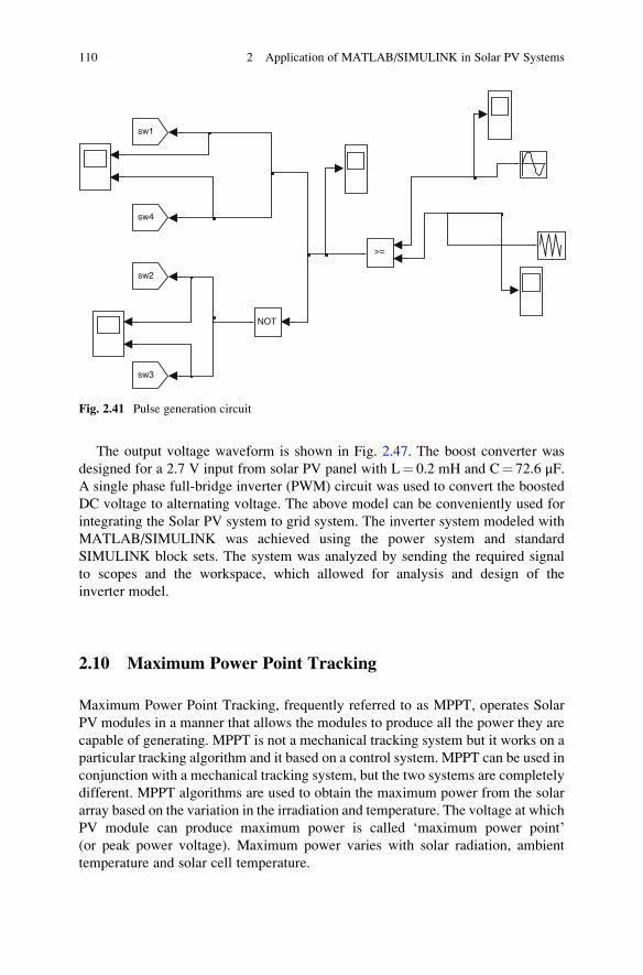
The output voltage waveform is shown in Fig. 2.47. The boost converter was
designed for a 2.7 V input from solar PV panel with L¼ 0.2 mH and C¼ 72.6 μF.A single phase full-bridge inverter (PWM) circuit was used to convert the boosted
DC voltage to alternating voltage. The above model can be conveniently used for
integrating the Solar PV system to grid system. The inverter system modeled with
MATLAB/SIMULINK was achieved using the power system and standard
SIMULINK block sets. The system was analyzed by sending the required signal
to scopes and the workspace, which allowed for analysis and design of the
inverter model.
2.10 Maximum Power Point Tracking
Maximum Power Point Tracking, frequently referred to as MPPT, operates Solar
PV modules in a manner that allows the modules to produce all the power they are
capable of generating. MPPT is not a mechanical tracking system but it works on a
particular tracking algorithm and it based on a control system. MPPT can be used in
conjunction with a mechanical tracking system, but the two systems are completely
different. MPPT algorithms are used to obtain the maximum power from the solar
array based on the variation in the irradiation and temperature. The voltage at which
PV module can produce maximum power is called ‘maximum power point’(or peak power voltage). Maximum power varies with solar radiation, ambient
temperature and solar cell temperature.
>=
NOT
sw3
sw2
sw1
sw4
Fig. 2.41 Pulse generation circuit
110 2 Application of MATLAB/SIMULINK in Solar PV Systems
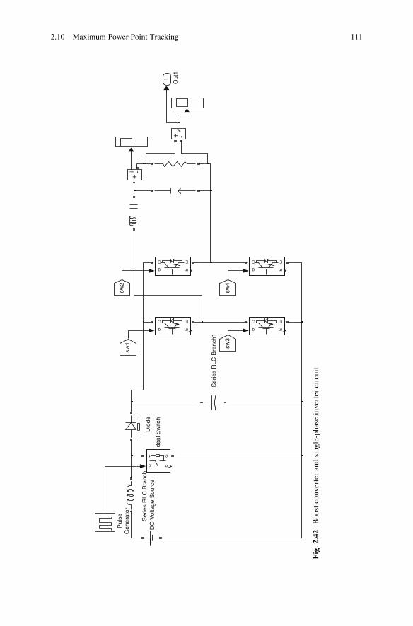
1 Out
1v
+ -
Ser
ies
RLC
Bra
nch1
Ser
ies
RLC
Bra
nch
Pul
seG
ener
ator
g m
1 2
Idea
l Sw
itch
g m
C E
g m
C E
g m
C E
g m
C E
sw3
sw4
sw2
sw1
Dio
deD
C V
olta
ge S
ourc
e
i+-
Fig.2.42
Boostconverterandsingle-phaseinvertercircuit
2.10 Maximum Power Point Tracking 111
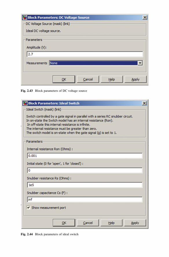
Fig. 2.43 Block parameters of DC voltage source
Fig. 2.44 Block parameters of ideal switch

Typical PV module produces power with maximum power voltage of around
17 V when measured at a cell temperature of 25 �C, it can drop to around 15 V on a
very hot day and it can also rise to 18 V on a very cold day. The major principle of
MPPT is to extract the maximum available power from PV module by making them
operate at the most efficient voltage. MPPT Algorithm is based on the simple logic
that, MPPT calculates the output of PV module, compares it to battery voltage then
Fig. 2.45 Block parameters of diode
2.10 Maximum Power Point Tracking 113
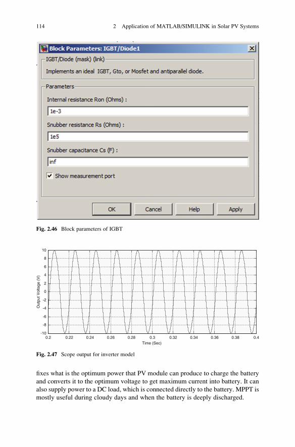
fixes what is the optimum power that PV module can produce to charge the battery
and converts it to the optimum voltage to get maximum current into battery. It can
also supply power to a DC load, which is connected directly to the battery. MPPT is
mostly useful during cloudy days and when the battery is deeply discharged.
Fig. 2.46 Block parameters of IGBT
0.2 0.22 0.24 0.26 0.28 0.3 0.32 0.34 0.36 0.38 0.4-10
-8
-6
-4
-2
0
2
4
6
8
10
Time (Sec)
Out
put V
olta
ge (
V)
Fig. 2.47 Scope output for inverter model
114 2 Application of MATLAB/SIMULINK in Solar PV Systems

2.10.1 MPPT Techniques
Over the past decades many methods to find the MPP have been developed. These
techniques differ in many aspects such as required sensors, complexity, cost, range
of effectiveness, convergence speed, correct tracking when irradiation and/or
temperature change, hardware needed for the implementation or popularity,
among others. Some of the most popular MPPT techniques are:
1. Perturb and Observe (hill climbing method).
2. Incremental Conductance method.
3. Fractional short circuit current.
4. Fractional open circuit voltage.
5. Fuzzy logic.
6. Neural networks.
7. Ripple Correlation Control.
8. Current Sweep.
9. DC-link capacitor droop control.
10. Load current or load voltage maximization.
11. dP/dV or dP/dI Feedback control.
Among several techniques mentioned, the Perturb and Observe (P&O) method
and the Incremental Conductance (InCond) algorithms are the most commonly
applied algorithms. Other techniques based on different principles include fuzzy
logic control, neural network, fractional open circuit voltage or short circuit current,
current sweep, etc. Most of these methods yield a local maximum and some, like the
fractional open circuit voltage or short circuit current, give an approximated MPP,
rather than an exact output. In normal conditions the V-P curve has only one
maximum. However, if the PV array is partially shaded, there are multiple maxima
in these curves. Both P&O and InCond algorithms are based on the “hill-climbing”
principle, which consists of moving the operation point of the PV array in the
direction in which the power increases. Hill-climbing techniques are the most
popular MPPT methods due to their ease of implementation and good performance
when the irradiation is constant. The advantages of both methods are simplicity and
requirement of low computational power. The drawbacks are: oscillations occur
around the MPP and they get lost and track the MPP in the wrong direction during
rapidly changing atmospheric conditions.
2.10.1.1 Perturb and Observe
In the P&O method only one voltage sensor is used to sense the PV array voltage
and hence the cost of implementation is less. The algorithm involves a perturbation
on the duty cycle of the power converter and a perturbation in the operating voltage
of the DC-link between the PV array and the power converter. Perturbing the
duty cycle of the power converter implies modifying the voltage of the DC-link
2.10 Maximum Power Point Tracking 115
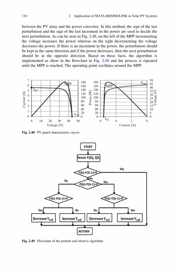
between the PV array and the power converter. In this method, the sign of the last
perturbation and the sign of the last increment in the power are used to decide the
next perturbation. As can be seen in Fig. 2.48, on the left of the MPP incrementing
the voltage increases the power whereas on the right decrementing the voltage
decreases the power. If there is an increment in the power, the perturbation should
be kept in the same direction and if the power decreases, then the next perturbation
should be in the opposite direction. Based on these facts, the algorithm is
implemented as show in the flowchart in Fig. 2.49 and the process is repeated
until the MPP is reached. The operating point oscillates around the MPP.
7 180160140120100806040200
1805045
35
25
15
50
10
20
30
40160140120100806040200
6
5
4
3
2
1
00 10 20 30
Voltage [V] Current [A]
Cur
rent
[A
]
Pow
er [W
]
Vol
tage
[V
]
40 50 6 4ISC
ISC
MPPMPP
VOC
VOC
2 0
Fig. 2.48 PV panel characteristic curves
Fig. 2.49 Flowchart of the perturb and observe algorithm
116 2 Application of MATLAB/SIMULINK in Solar PV Systems

The time complexity of this algorithm is very less but on reaching very close
to the MPP it doesn’t stop at the MPP and keeps on perturbing on both the
directions. To avoid such a condition, an appropriate error limit can be set or a
wait function can be used to stop the increase in time complexity of the algorithm.
However the method does not take account of the rapid change of irradiation level
(due to which MPPT changes) and considers it as a change in MPP due to
perturbation and ends up calculating the wrong MPP. To avoid this problem we
can use incremental conductance method.
2.10.1.2 Incremental Conductance
The incremental conductance algorithm uses two voltage and current sensors
to sense the output voltage and current of the PV array. In incremental conduc-
tance method the array terminal voltage is always adjusted according to the MPP
voltage it is based on the incremental and instantaneous conductance of the
PV module.
Figure 2.50 shows that the slope of the P-V array power curve is zero at
The MPP, increasing on the left of the MPP and decreasing on the Right hand
side of the MPP. The basic equations of this method are as follows.
dI
dV¼ � I
VAt MPP
dI
dV> � I
VLeft of MPP
dI
dV< � I
VRight of MPP
ð2:11Þ
where I and V are P-V array output current and voltage respectively. The left hand
side of equations represents incremental conductance of P-V module and the right
hand side represents the instantaneous conductance. When the ratio of change
in output conductance is equal to the negative output conductance, the solar array
Left
P
dPdV
>0
dPMPP
Right
dV=0
dPdV
V
<0
Fig. 2.50 Basic idea of
incremental conductance
method on a P-V curve of
solar module
2.10 Maximum Power Point Tracking 117

will operate at the maximum power point. This method exploits the assumption
of the ratio of change in output conductance is equal to the negative output
Instantaneous conductance. We have,
P ¼ VI
Applying the chain rule for the derivative of products yields to
∂P=∂V ¼ ∂ VIð Þ½ �=∂V ð2:12Þ
At MPP, as ∂P=∂V ¼ 0
The above equation could be written in terms of array voltage V and array
current I as
∂P=∂V ¼ �I=V ð2:13Þ
The MPPT regulates the PWM control signal of the DC – to – DC boost converter
until the condition: (∂I/∂V) + (I/V)¼ 0 is satisfied. In this method the peak power
of the module lies at above 98 % of its incremental conductance. The Flow chart of
incremental conductance MPPT is shown in Fig. 2.51.
In both P&O and InCond schemes, the speed of occurrence of MPP depends
on the size of the increment of the reference voltage. The drawbacks of these
Fig. 2.51 Flow chart for incremental conductance algorithm
118 2 Application of MATLAB/SIMULINK in Solar PV Systems
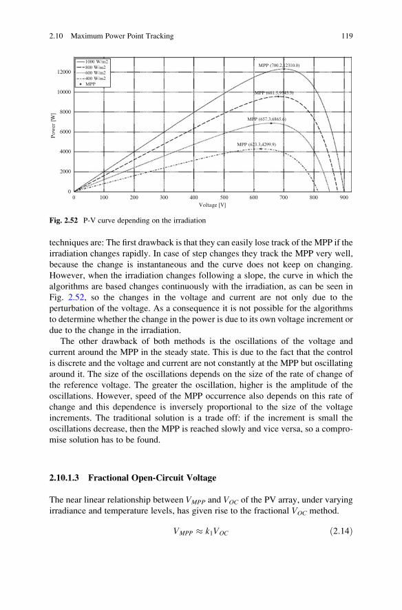
techniques are: The first drawback is that they can easily lose track of the MPP if the
irradiation changes rapidly. In case of step changes they track the MPP very well,
because the change is instantaneous and the curve does not keep on changing.
However, when the irradiation changes following a slope, the curve in which the
algorithms are based changes continuously with the irradiation, as can be seen in
Fig. 2.52, so the changes in the voltage and current are not only due to the
perturbation of the voltage. As a consequence it is not possible for the algorithms
to determine whether the change in the power is due to its own voltage increment or
due to the change in the irradiation.
The other drawback of both methods is the oscillations of the voltage and
current around the MPP in the steady state. This is due to the fact that the control
is discrete and the voltage and current are not constantly at the MPP but oscillating
around it. The size of the oscillations depends on the size of the rate of change of
the reference voltage. The greater the oscillation, higher is the amplitude of the
oscillations. However, speed of the MPP occurrence also depends on this rate of
change and this dependence is inversely proportional to the size of the voltage
increments. The traditional solution is a trade off: if the increment is small the
oscillations decrease, then the MPP is reached slowly and vice versa, so a compro-
mise solution has to be found.
2.10.1.3 Fractional Open-Circuit Voltage
The near linear relationship between VMPP and VOC of the PV array, under varying
irradiance and temperature levels, has given rise to the fractional VOC method.
VMPP � k1VOC ð2:14Þ
12000
10000
8000
6000
4000
2000
00 100 200 300 400 500
Voltage [V]
Pow
er [W
]
600 700 800 900
1000 W/m2800 W/m2600 W/m2400 W/m2MPP
MPP (681.5,9545.3)
MPP (657.3,6865.6)
MPP (623.3,4299.9)
MPP (700.2,12310.0)
Fig. 2.52 P-V curve depending on the irradiation
2.10 Maximum Power Point Tracking 119

where k1 is a constant of proportionality. Since k1 is dependent on the characteris-
tics of the PV array being used, it usually has to be computed beforehand by
empirically determining VMPP and VOC for the specific PV array at different
irradiance and temperature levels. The factor k1 has been reported to be between
0.71 and 0.78. Once k1 is known, VMPP can be computed using (2.14) with VOC
measured periodically by momentarily shutting down the power converter.
However, this incurs some disadvantages, including temporary loss of power.
To prevent this, pilot cells are used from which VOC can be obtained. These pilot
cells must be carefully chosen to closely represent the characteristics of the PV
array. Once VMPP has been approximated, a closed loop control on the array power
converter can be used to asymptotically reach this desired voltage. Since (2.14) is
only an approximation, the PV array technically never operates at the MPP.
Depending on the application of the PV system, this can sometimes be adequate.
Even if fractional VOC is not a true MPPT technique, it is very easy and cheap to
implement as it does not necessarily require DSP or microcontroller control.
However, k1 is no more valid in the presence of partial shading (which causes
multiple local maxima) of the PV array and proposes sweeping the PV array voltage
to update k1. This obviously adds to the implementation complexity and incurs
more power loss.
2.10.1.4 Fractional Short-Circuit Current
Fractional ISC results from the fact that, under varying atmospheric conditions, IMPP
is approximately linearly related to the ISC of the PV array.
IMPP � k2ISC ð2:15Þ
where k2 is a proportionality constant. Just like in the fractional VOC technique, k2has to be determined according to the PV array in use. The constant k2 is generallyfound to be between 0.78 and 0.92. Measuring ISC during operation is pro-
blematic. An additional switch usually has to be added to the power converter
to periodically short the PV array so that ISC can be measured using a current
sensor. This increases the number of components and cost. Power output is not
only reduced when finding ISC but also because the MPP is never perfectly
matched as suggested by (2.15). The variable k2 can be compensated such that
the MPP is better tracked while atmospheric conditions change. To guarantee
proper MPPT in the presence of multiple local maxima, the PV array voltage from
open-circuit to short-circuit periodically sweeps to update k2. Most of the PV
systems using fractional ISC in the literature use a DSP, while a few systems use a
simple current feedback control loop instead.
120 2 Application of MATLAB/SIMULINK in Solar PV Systems
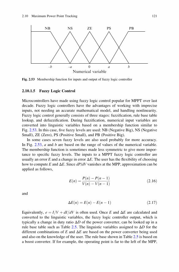
2.10.1.5 Fuzzy Logic Control
Microcontrollers have made using fuzzy logic control popular for MPPT over last
decade. Fuzzy logic controllers have the advantages of working with imprecise
inputs, not needing an accurate mathematical model, and handling nonlinearity.
Fuzzy logic control generally consists of three stages: fuzzification, rule base table
lookup, and defuzzification. During fuzzification, numerical input variables are
converted into linguistic variables based on a membership function similar to
Fig. 2.53. In this case, five fuzzy levels are used: NB (Negative Big), NS (Negative
Small), ZE (Zero), PS (Positive Small), and PB (Positive Big).
In some cases seven fuzzy levels are also used probably for more accuracy.
In Fig. 2.53, a and b are based on the range of values of the numerical variable.
The membership function is sometimes made less symmetric to give more impor-
tance to specific fuzzy levels. The inputs to a MPPT fuzzy logic controller are
usually an error E and a change in error ΔE. The user has the flexibility of choosinghow to compute E and ΔE. Since dP/dV vanishes at the MPP, approximation can be
applied as follows,
E nð Þ ¼ P nð Þ � P n� 1ð ÞV nð Þ � V n� 1ð Þ ð2:16Þ
and
ΔE nð Þ ¼ E nð Þ � E n� 1ð Þ ð2:17Þ
Equivalently, e ¼ I=V þ dI=dV is often used. Once E and ΔE are calculated and
converted to the linguistic variables, the fuzzy logic controller output, which is
typically a change in duty ratio ΔD of the power converter, can be looked up in a
rule base table such as Table 2.5. The linguistic variables assigned to ΔD for the
different combinations of E and ΔE are based on the power converter being used
and also on the knowledge of the user. The rule base shown in Table 2.5 is based on
a boost converter. If for example, the operating point is far to the left of the MPP,
Numerical variable
NB NS ZE PS PB
0–a a–b b
Fig. 2.53 Membership function for inputs and output of fuzzy logic controller
2.10 Maximum Power Point Tracking 121
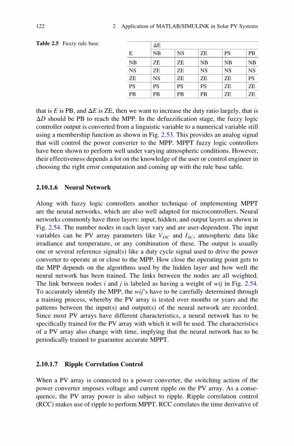
that is E is PB, and ΔE is ZE, then we want to increase the duty ratio largely, that is
ΔD should be PB to reach the MPP. In the defuzzification stage, the fuzzy logic
controller output is converted from a linguistic variable to a numerical variable still
using a membership function as shown in Fig. 2.53. This provides an analog signal
that will control the power converter to the MPP. MPPT fuzzy logic controllers
have been shown to perform well under varying atmospheric conditions. However,
their effectiveness depends a lot on the knowledge of the user or control engineer in
choosing the right error computation and coming up with the rule base table.
2.10.1.6 Neural Network
Along with fuzzy logic controllers another technique of implementing MPPT
are the neural networks, which are also well adapted for microcontrollers. Neural
networks commonly have three layers: input, hidden, and output layers as shown in
Fig. 2.54. The number nodes in each layer vary and are user-dependent. The input
variables can be PV array parameters like VOC and ISC, atmospheric data like
irradiance and temperature, or any combination of these. The output is usually
one or several reference signal(s) like a duty cycle signal used to drive the power
converter to operate at or close to the MPP. How close the operating point gets to
the MPP depends on the algorithms used by the hidden layer and how well the
neural network has been trained. The links between the nodes are all weighted.
The link between nodes i and j is labeled as having a weight of wij in Fig. 2.54.
To accurately identify the MPP, the wij’s have to be carefully determined through
a training process, whereby the PV array is tested over months or years and the
patterns between the input(s) and output(s) of the neural network are recorded.
Since most PV arrays have different characteristics, a neural network has to be
specifically trained for the PV array with which it will be used. The characteristics
of a PV array also change with time, implying that the neural network has to be
periodically trained to guarantee accurate MPPT.
2.10.1.7 Ripple Correlation Control
When a PV array is connected to a power converter, the switching action of the
power converter imposes voltage and current ripple on the PV array. As a conse-
quence, the PV array power is also subject to ripple. Ripple correlation control
(RCC) makes use of ripple to performMPPT. RCC correlates the time derivative of
Table 2.5 Fuzzy rule base
E
ΔENB NS ZE PS PB
NB ZE ZE NB NB NB
NS ZE ZE NS NS NS
ZE NS ZE ZE ZE PS
PS PS PS PS ZE ZE
PB PB PB PB ZE ZE
122 2 Application of MATLAB/SIMULINK in Solar PV Systems
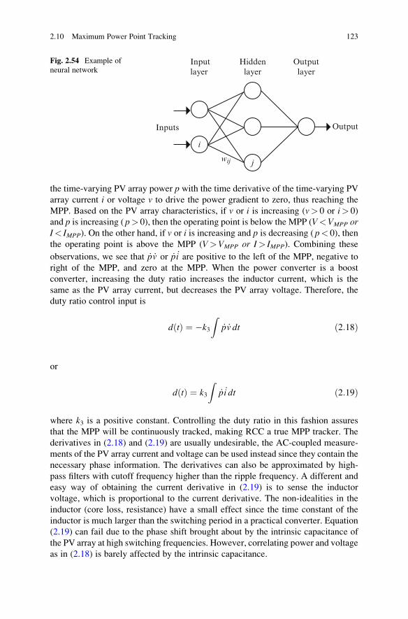
the time-varying PV array power p with the time derivative of the time-varying PV
array current i or voltage v to drive the power gradient to zero, thus reaching the
MPP. Based on the PV array characteristics, if v or i is increasing (v> 0 or i> 0)
and p is increasing ( p> 0), then the operating point is below the MPP (V<VMPP orI< IMPP). On the other hand, if v or i is increasing and p is decreasing ( p< 0), then
the operating point is above the MPP (V>VMPP or I> IMPP). Combining these
observations, we see that _p _v or _p _i are positive to the left of the MPP, negative to
right of the MPP, and zero at the MPP. When the power converter is a boost
converter, increasing the duty ratio increases the inductor current, which is the
same as the PV array current, but decreases the PV array voltage. Therefore, the
duty ratio control input is
d tð Þ ¼ �k3
Z_p _v dt ð2:18Þ
or
d tð Þ ¼ k3
Z_p _i dt ð2:19Þ
where k3 is a positive constant. Controlling the duty ratio in this fashion assures
that the MPP will be continuously tracked, making RCC a true MPP tracker. The
derivatives in (2.18) and (2.19) are usually undesirable, the AC-coupled measure-
ments of the PV array current and voltage can be used instead since they contain the
necessary phase information. The derivatives can also be approximated by high-
pass filters with cutoff frequency higher than the ripple frequency. A different and
easy way of obtaining the current derivative in (2.19) is to sense the inductor
voltage, which is proportional to the current derivative. The non-idealities in the
inductor (core loss, resistance) have a small effect since the time constant of the
inductor is much larger than the switching period in a practical converter. Equation
(2.19) can fail due to the phase shift brought about by the intrinsic capacitance of
the PV array at high switching frequencies. However, correlating power and voltage
as in (2.18) is barely affected by the intrinsic capacitance.
Inputlayer
Hiddenlayer
Outputlayer
OutputInputs
i
jwij
Fig. 2.54 Example of
neural network
2.10 Maximum Power Point Tracking 123
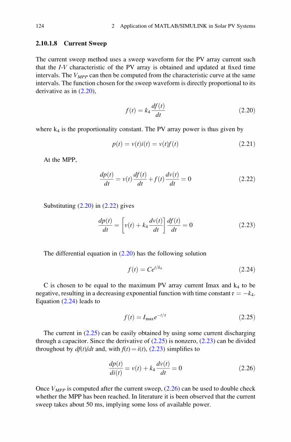
2.10.1.8 Current Sweep
The current sweep method uses a sweep waveform for the PV array current such
that the I-V characteristic of the PV array is obtained and updated at fixed time
intervals. The VMPP can then be computed from the characteristic curve at the same
intervals. The function chosen for the sweep waveform is directly proportional to its
derivative as in (2.20),
f tð Þ ¼ k4df tð Þdt
ð2:20Þ
where k4 is the proportionality constant. The PV array power is thus given by
p tð Þ ¼ v tð Þi tð Þ ¼ v tð Þf tð Þ ð2:21Þ
At the MPP,
dp tð Þdt
¼ v tð Þ df tð Þdt
þ f tð Þ dv tð Þdt
¼ 0 ð2:22Þ
Substituting (2.20) in (2.22) gives
dp tð Þdt
¼ v tð Þ þ k4dv tð Þdt
� �df tð Þdt
¼ 0 ð2:23Þ
The differential equation in (2.20) has the following solution
f tð Þ ¼ Cet=k4 ð2:24Þ
C is chosen to be equal to the maximum PV array current Imax and k4 to be
negative, resulting in a decreasing exponential function with time constant τ ¼ �k4.Equation (2.24) leads to
f tð Þ ¼ Imaxe�t=τ ð2:25Þ
The current in (2.25) can be easily obtained by using some current discharging
through a capacitor. Since the derivative of (2.25) is nonzero, (2.23) can be divided
throughout by df(t)/dt and, with f(t)¼ i(t), (2.23) simplifies to
dp tð Þdi tð Þ ¼ v tð Þ þ k4
dv tð Þdt
¼ 0 ð2:26Þ
Once VMPP is computed after the current sweep, (2.26) can be used to double check
whether the MPP has been reached. In literature it is been observed that the current
sweep takes about 50 ms, implying some loss of available power.
124 2 Application of MATLAB/SIMULINK in Solar PV Systems

2.10.1.9 DC Link Capacitor Droop Control
DC-link capacitor droop control is a MPPT technique that is specifically designed
to work with a PV system that is connected in parallel with an AC system line as
shown in Fig. 2.55. The duty ratio of an ideal boost converter is given by
d ¼ 1� V=Vlink ð2:27Þ
where V is the voltage across the PV array and Vlink is the voltage across the DC-
link. If Vlink is kept constant, increasing the current going in the inverter increases
the power coming out of the boost converter and consequently increases the power
coming out of the PV array. While the current is increasing, the voltage Vlink can be
kept constant as long as the power required by the inverter does not exceed the
maximum power available from the PV array. If that is not the case, Vlink starts
drooping. Right before that point, the current control command Ipeak of the inverteris at its maximum and the PV array operates at the MPP. The AC system line
current is feedback to prevent Vlink from drooping and d is optimized to bring Ipeakto its maximum, thus achieving MPPT. DC-link capacitor droop control does not
require the computation of the PV array power, but its response deteriorates when
compared to a method that detects the power directly; this is because its response
directly depends on the response of the DC voltage control loop of the inverter. This
control scheme can be easily implemented with analog operational amplifiers and
decision making logic units.
2.10.1.10 Load Current or Load Voltage Maximization
The purpose of MPPT techniques is to maximize the power coming out of
a PV array. When the PV array is connected to a power converter, maximizing
Inverter
ControlMPPT
BoostConverter
PV Array DC Link AC System Line
d
V
Vlink
Ipeak
Fig. 2.55 Topology for DC-link capacitor droop control
2.10 Maximum Power Point Tracking 125
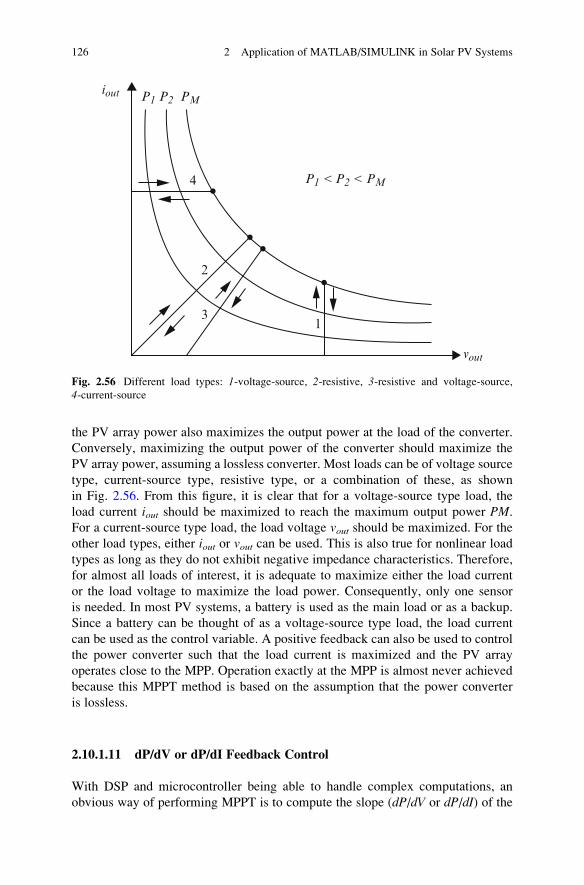
the PV array power also maximizes the output power at the load of the converter.
Conversely, maximizing the output power of the converter should maximize the
PV array power, assuming a lossless converter. Most loads can be of voltage source
type, current-source type, resistive type, or a combination of these, as shown
in Fig. 2.56. From this figure, it is clear that for a voltage-source type load, the
load current iout should be maximized to reach the maximum output power PM.
For a current-source type load, the load voltage vout should be maximized. For the
other load types, either iout or vout can be used. This is also true for nonlinear load
types as long as they do not exhibit negative impedance characteristics. Therefore,
for almost all loads of interest, it is adequate to maximize either the load current
or the load voltage to maximize the load power. Consequently, only one sensor
is needed. In most PV systems, a battery is used as the main load or as a backup.
Since a battery can be thought of as a voltage-source type load, the load current
can be used as the control variable. A positive feedback can also be used to control
the power converter such that the load current is maximized and the PV array
operates close to the MPP. Operation exactly at the MPP is almost never achieved
because this MPPT method is based on the assumption that the power converter
is lossless.
2.10.1.11 dP/dV or dP/dI Feedback Control
With DSP and microcontroller being able to handle complex computations, an
obvious way of performing MPPT is to compute the slope (dP/dV or dP/dI) of the
13
2
4 P1
P1iout
vout
P2
P2
PM
PM
< <
Fig. 2.56 Different load types: 1-voltage-source, 2-resistive, 3-resistive and voltage-source,
4-current-source
126 2 Application of MATLAB/SIMULINK in Solar PV Systems

PV power curve and feed it back to the power converter with some control to drive
it to zero. There are several methods to compute the slope. dP/dV can be computed
and its sign can be stored for the past few cycles. Based on these signs, the duty ratio
of the power converter is either incremented or decremented to reach the voltage-
source, 4-current-source. A dynamic step size is used to improve the transient
response of the system. Linearization based method can also be used to compute
dP/dV. Sometimes sampling and data conversion with subsequent digital division
of power and voltage are also applied to approximate dP/dV. dP/dI can then be
integrated together with an adaptive gain to improve the transient response. The PV
array voltage is periodically incremented or decremented and ΔP/ΔV is compared
to a marginal error until the MPP is reached. Convergence to the MPP was shown to
occur in tens of milliseconds.
With so many MPPT techniques available to PV system users, it might not
be obvious for the latter to choose which one better suits their application needs.
The main aspects of the MPPT techniques to be taken into consideration are
highlighted in the following subsections.
Implementation
The ease of implementation is an important factor in deciding which MPPT
technique to use. However, this greatly depends on the end-users’ knowledge.
Some might be more familiar with analog circuitry, in which case, fractional ISCor VOC, RCC, and load current or voltage maximization are good options. Others
might be willing to work with digital circuitry, even if that may require the use of
software and programming. Then, their selection should include hill-climbing/
P&O, IncCond, fuzzy logic control, neural network, and dP/dV or dP/dI feedbackcontrol. Furthermore, a few of the MPPT techniques only apply to specific topol-
ogies. For example, the DC-link capacitor droop control works with the system
shown in Fig. 2.55 and the OCC MPPT works with a single-stage inverter.
Sensors
The number of sensors required to implement MPPT also affects the decision
process. Most of the time, it is easier and more reliable to measure voltage than
current. Moreover, current sensors are usually expensive and bulky. This might be
inconvenient in systems that consist of several PV arrays with separate MPP
trackers. In such cases, it might be wise to use MPPT methods that require only
one sensor or that can estimate the current from the voltage. It is also uncommon to
find sensors that measure irradiance levels, as needed in the linear current control
and the IMPP and VMPP computation methods.
2.10 Maximum Power Point Tracking 127

Multiple Local Maxima
The occurrence of multiple local maxima due to partial shading of the PV array
(s) can be a real hindrance to the proper functioning of a MPP tracker. Considerable
power loss can be incurred if a local maximum is tracked instead of the real MPP.
As mentioned previously, the current sweep and the state-based methods should
track the true MPP even in the presence of multiple local maxima. However, the
other methods require an additional initial stage to bypass the unwanted local
maxima and bring operation to close the real MPP.
Costs
It is hard to mention the monetary costs of every single MPPT technique unless it is
built and implemented. However, a good costs comparison can be made by know-
ing whether the technique is analog or digital, whether it requires software and
programming, and the number of sensors. Analog implementation is generally
cheaper than digital, which normally involves a microcontroller that needs to be
programmed. Eliminating current sensors considerably drops the costs.
Applications
Different MPPT techniques discussed above will suit different applications.
For example, in space satellites and orbital stations that involve large amount of
money, the costs and complexity of the MPP tracker are not as important as its
performance and reliability. The tracker should be able to continuously track
the true MPP in minimum amount of time and should not require periodic tuning.
In this case, hill climbing/P&O, IncCond, and RCC are appropriate. Solar vehicles
would mostly require fast convergence to the MPP. Fuzzy logic control, neural
network, and RCC are good options in this case. Since the load in solar vehicles
consists mainly of batteries, load current or voltage maximization should also be
considered. The goal when using PV arrays in residential areas is to minimize the
payback time and to do so, it is essential to constantly and quickly track the MPP.
Since partial shading (from trees and other buildings) can be an issue, the MPPT
should be capable of bypassing multiple local maxima. Therefore, the two-stage
IncCond and the current sweep methods are suitable. Since a residential system
might also include an inverter, the OCC MPPT can also be used. PV systems used
for street lighting only consist in charging up batteries during the day. They do not
necessarily need tight constraints; easy and cheap implementation might be more
important, making fractional VOC or ISC viable. Table 2.6 summarizes the major
characteristics of all the MPPT techniques.
128 2 Application of MATLAB/SIMULINK in Solar PV Systems
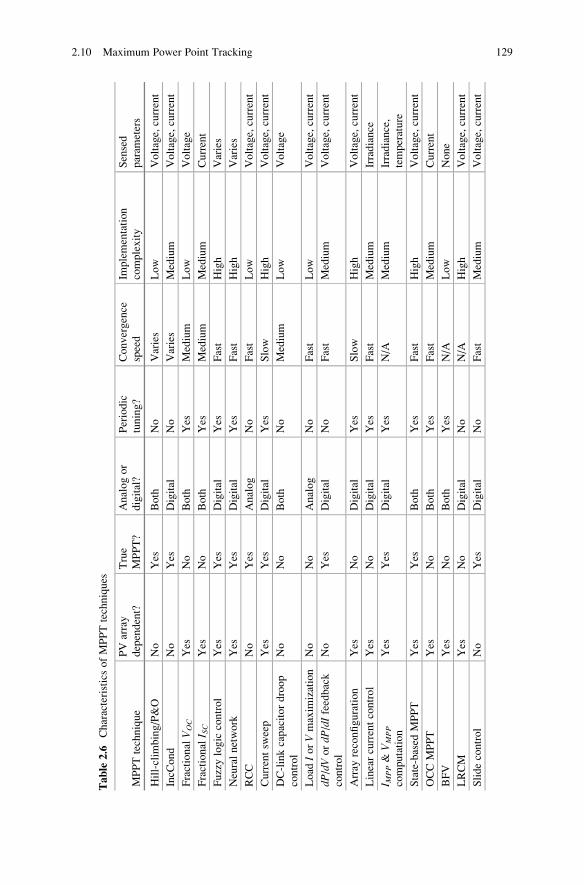
Table
2.6
CharacteristicsofMPPTtechniques
MPPTtechnique
PVarray
dependent?
True
MPPT?
Analogor
digital?
Periodic
tuning?
Convergence
speed
Implementation
complexity
Sensed
param
eters
Hill-clim
bing/P&O
No
Yes
Both
No
Varies
Low
Voltage,current
IncC
ond
No
Yes
Digital
No
Varies
Medium
Voltage,current
Fractional
VOC
Yes
No
Both
Yes
Medium
Low
Voltage
Fractional
I SC
Yes
No
Both
Yes
Medium
Medium
Current
Fuzzylogic
control
Yes
Yes
Digital
Yes
Fast
High
Varies
Neuralnetwork
Yes
Yes
Digital
Yes
Fast
High
Varies
RCC
No
Yes
Analog
No
Fast
Low
Voltage,current
Currentsw
eep
Yes
Yes
Digital
Yes
Slow
High
Voltage,current
DC-linkcapacitordroop
control
No
No
Both
No
Medium
Low
Voltage
Load
IorVmaxim
ization
No
No
Analog
No
Fast
Low
Voltage,current
dP/dVordP/dIfeedback
control
No
Yes
Digital
No
Fast
Medium
Voltage,current
Array
reconfiguration
Yes
No
Digital
Yes
Slow
High
Voltage,current
Linearcurrentcontrol
Yes
No
Digital
Yes
Fast
Medium
Irradiance
I MPP&
VMPP
computation
Yes
Yes
Digital
Yes
N/A
Medium
Irradiance,
temperature
State-based
MPPT
Yes
Yes
Both
Yes
Fast
High
Voltage,current
OCCMPPT
Yes
No
Both
Yes
Fast
Medium
Current
BFV
Yes
No
Both
Yes
N/A
Low
None
LRCM
Yes
No
Digital
No
N/A
High
Voltage,current
Slidecontrol
No
Yes
Digital
No
Fast
Medium
Voltage,current
2.10 Maximum Power Point Tracking 129

2.10.2 MATLAB/SIMULINK Implementationof Perturb and Observe Method
The detailed block diagram of the P&O algorithm mentioned above is constructed
using MATLAB/SIMULINK and the model is shown in Fig. 2.57. Here the voltage
and current inputs are sensed to compute power as shown. A saturation limit is set
to monitor the increase or decrease in voltage in order to avoid oscillations in
the MPP.
2.10.3 MATLAB/SIMULINK Model of the IncrementalConductance Method
The MATLAB/SIMULINK model of the incremental conductance method is
shown in Fig. 2.58.
The duty cycle in both P&O and the InCond algorithms can be adjusted as shown
in Fig. 2.59.
2.10.4 PV Module with MPPT Techniques
The SIMULINK model for the MPPT algorithm using incremental conductance
(If P&O algorithm is required the block can be replaced accordingly) is shown in
Fig. 2.60. The PV module is added from Fig. 2.9.
130 2 Application of MATLAB/SIMULINK in Solar PV Systems
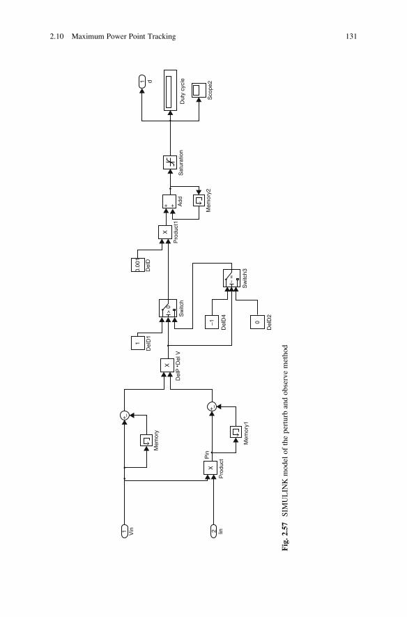
Vin1
1
–1 0
2 lin
Mem
ory
Pin
X
XX
Pro
duct
Mem
ory1
+
+
–
–
Del
D1
Del
D
0.00
1
Del
D4
Del
D2
Del
P •
Del
VS
witc
h
> 0
~ =
Pro
duct
1A
ddS
atur
atio
n
Sw
itch3
Mem
ory2
1 d
Dut
y cy
cle
Sco
pe2
+ +
Fig.2.57
SIM
ULIN
Kmodel
oftheperturb
andobservemethod
2.10 Maximum Power Point Tracking 131

1 2Vin lin
Mem
ory
Mem
ory2
Mem
ory3
Mem
ory1
X
x
x+ +
÷ ÷x
delP
Del
D1
–10.
001
Del
D4
Del
D2
Del
D
+ –+
+
–
–
Sw
itch
Sw
itch3P
rodu
ct1
Add
delV
/del
P
delI/
delP
01
~=
>0
Sat
urat
ion1
Dut
y cy
cle
Sco
pe2d1
Fig.2.58
SIM
ULIN
Kmodel
ofincrem
entalconductance
method
132 2 Application of MATLAB/SIMULINK in Solar PV Systems
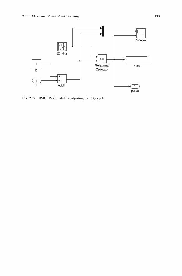
20 kHz
Add1d
D
1
+–1
RelationalOperator
Scope
duty
1
>=
pulse
Fig. 2.59 SIMULINK model for adjusting the duty cycle
2.10 Maximum Power Point Tracking 133
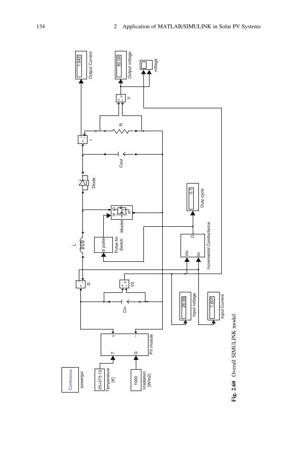
pow
ergu
i
Con
tinuo
us
25+
273.
15
Tem
pera
ture
[K]
1000
Irra
diat
ion
[W/m
2]P
V m
odul
e
GT+ –
Cin
V2v
+ –
Inpu
t vol
tage
26.5
6
7.60
7
Inpu
t Cur
rent
Incr
emen
tal C
ondu
ctan
ce
Vin
linD
uty
cycl
e
0.7
Pul
se fo
rS
witc
hM
osfe
t
puls
ed
Dio
de
Cou
t
+
+
–
–
i
I
R
Vv
Out
put v
olta
ge
82.0
9
volta
ge
Out
put C
urre
nt
1.64
2
Sg
D
L
I2
–+
i
D
Fig.2.60
OverallSIM
ULIN
Kmodel
134 2 Application of MATLAB/SIMULINK in Solar PV Systems
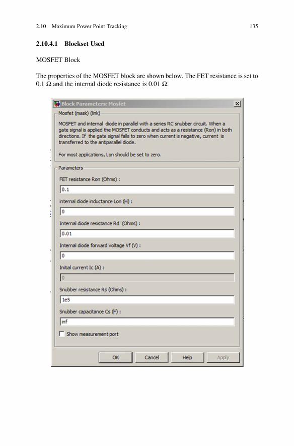
2.10.4.1 Blockset Used
MOSFET Block
The properties of the MOSFET block are shown below. The FET resistance is set to
0.1 Ω and the internal diode resistance is 0.01 Ω.
2.10 Maximum Power Point Tracking 135
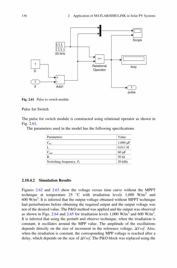
Pulse for Switch
The pulse for switch module is constructed using relational operator as shown in
Fig. 2.61.
The parameters used in the model has the following specifications
Parameters Value
Cin 1,000 μFL 0.011 H
Cout 60 μFR 50 ΩSwitching frequency, Fs 20 kHz
2.10.4.2 Simulation Results
Figures 2.62 and 2.63 show the voltage versus time curve without the MPPT
technique at temperature 25 �C with irradiation levels 1,000 W/m2 and
600 W/m2. It is inferred that the output voltage obtained without MPPT technique
had perturbations before obtaining the required output and the output voltage was
not of the desired value. The P&O method was applied and the output was observed
as shown in Figs. 2.64 and 2.65 for irradiation levels 1,000 W/m2 and 600 W/m2.
It is inferred that using the perturb and observe technique, when the irradiation is
constant, it oscillates around the MPP value. The amplitude of the oscillations
depends directly on the size of increment in the reference voltage, ΔVref. Also,when the irradiation is constant, the corresponding MPP voltage is reached after a
delay, which depends on the size of ΔVref. The P&O block was replaced using the
1
1
D
d Add1
+–
20 kHz
RelationalOperator
Scope
duty
1
pulse
>=
Fig. 2.61 Pulse to switch module
136 2 Application of MATLAB/SIMULINK in Solar PV Systems

Fig. 2.63 Voltage versus time curve without MPPT technique at temperature 25 �C and irradiance
600 W/m2
Fig. 2.62 Voltage versus time curve without MPPT technique at temperature 25 �C and irradiance
1,000 W/m2
Fig. 2.64 Voltage versus time curve with P&O MPPT technique with temperature 25 �C and
irradiance 1,000 W/m2

InCond technique and the output was observed as shown in Figs. 2.66 and 2.67.
The results are almost practically the same. Simulations were carried out by varying
the irradiation levels from 1,000W/m2 to 600W/m2. Figure 2.68 shows the Voltage
versus Time curve with P&O MPPT technique and Fig. 2.69 shows the Voltage
versus Time curve with In Cond MPPT technique. In this case the tracking is
adequate, which demonstrates that irradiation step changes do not pose a challenge
to the hill-climbing algorithms and are not suitable for testing MPPT. As expected,
the convergence speed, i.e. how fast the steady state is reached, and the amplitude
of the oscillations are a trade off, as both cannot be improved at the same time: if
one is reduced the other increases, because both depend directly on the size of the
voltage increment.
Fig. 2.65 Voltage versus time curve with P&O MPPT technique with temperature 25 �C and
irradiance 600 W/m2
Fig. 2.66 Voltage versus time curve with In Cond MPPT technique with temperature 25 �C and
irradiance 1,000 W/m2
138 2 Application of MATLAB/SIMULINK in Solar PV Systems
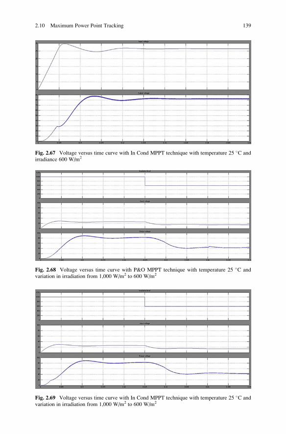
Fig. 2.67 Voltage versus time curve with In Cond MPPT technique with temperature 25 �C and
irradiance 600 W/m2
Fig. 2.68 Voltage versus time curve with P&O MPPT technique with temperature 25 �C and
variation in irradiation from 1,000 W/m2 to 600 W/m2
Fig. 2.69 Voltage versus time curve with In Cond MPPT technique with temperature 25 �C and
variation in irradiation from 1,000 W/m2 to 600 W/m2
2.10 Maximum Power Point Tracking 139

2.11 Summary
Solar PV is used primarily for grid-connected electricity to operate residential
appliances, commercial equipment, lighting and air conditioning for all types of
buildings. Through stand-alone systems and the use of batteries, it is also well
suited for remote regions where there is no electricity source. Solar PV panels can
be ground mounted, installed on building rooftops or designed into building
materials at the point of manufacturing. This chapter discussed the solar PV
array, batteries, charge controllers, inverters, power conditioning unit and MPPT
techniques along with their MATLAB/SIMULINK modules. The future will see
everyday objects such as clothing, the rooftops of cars and even roads themselves
turned into power-generating solar collectors.
Review Questions1. Mention the major components of a PV system.
2. Differentiate between grid connected and stand-alone PV systems.
3. What is the need for batteries in stand-alone PV systems?
4. What are the considerations for installing PV arrays on rooftops?
5. List the consequences of shading in PV arrays.
6. How are stand-alone PV systems sized?
7. Differentiate between PWM charge controller and MPPT charge controller.
8. Develop a MATLAB/SIMULINK model for a PV system using micro
inverters.
9. Design a full bridge inverter using MATLAB/SIMULINK.
10. Design and simulate a PV module using fuzzy based MPPT algorithm using
MATLAB/SIMULINK.
Bibliography
Ahmed MM, Sulaiman M (2003) Design and proper sizing of solar energy schemes for electricity
production in Malaysia. National Power and Energy Conference 2003, pp 268–271
Akhter R, Hoque A (2008) Analysis of a PWM boost inverter for solar home application. World
Acad Sci Eng Technol 23
Anegawa T (2010) Characteristics of CHAdeMO quick charging system. In: Proceedings of the
EVS-25 Shenzhen, 5–9 Nov 2010
Ardente F, Beccali G, Cellura M (2004) Life cycle assessment of a solar thermal collector. Science
Direct
Atlas H, Sharaf AM (2007) A photovoltaic array simulation model for matlab-simulink GUI
environment. In: Proceeedings of IEEE international conference on clean electrical power,
ICCEP 2007, Capri
AVA Solar website (2008) IEEE standard for interconnecting distributed resources with electric
power systems, New York: IEEE, IEEE Std.1547–2003. http://www.avasolar.com. Accessed
June 2008.
140 2 Application of MATLAB/SIMULINK in Solar PV Systems
Ayob SM, Yee CH, Muhamad ND, Jusoh A (2005) A new hybrid multilevel inverter topology with
harmonics profile improvement. IEEE Trans Power Electron Drives Syst, ISSN: 0-7803-9296-
5/05, pp 999–1002
Baldsing et al (1991) Lead-acid batteries for remote area energy storage. CSIRO Australia, Jan
1991
Banerjee S, Jeevananathan (2010) Modeling of PV array and performance enhancement by MPPT
algorithm. Int J Comput Appl 7:35–39 (0975–8887)
Bechtel National (1980) Handbook for battery energy storage in photovoltaic power systems, Final
report, SAND80-7022, Feb 1980
Borowy BS, Salameh ZM (1996) Methodology for optimally sizing the combination of a battery
bank and PV array in a wind/PV hybrid system. IEEE Trans Energy Conv 11(2):367–375
“Buck Converter Design Example”, Microchip WebSeminor, Microchip Technology Incorpo-
rated. All Rights Reserved (2006). Microchip Web Sites: www.microchip.com/smps
Calais M, Agelidis V (1998) Multilevel converters for single phase grid connected photovoltaic
systems, an overview. IEEE Int Symp Ind Electron 7–10:224–229
Cavalcanti MC, de Oliveira KC, Neves FAS, Azevedo GMS (2010) Modulation techniques to
eliminate leakage currents in transformer less three-phase photovoltaic systems. IEEE Trans
Ind Electron 57(4)
Chang HC, Liaw CM (2009) Development of compact switched reluctance motor drive for EV
propulsion with voltage-boosting and PFC charging capabilities. IEEE Trans Veh Technol
58:3198–3215
Chen A, He X (2006) Research on hybrid-clamped multilevel inverter topologies. IEEE Trans Ind
Electron 53(6):1898–1906
Chowdhury AA, Koval DO (2005) Impact of photovoltaic power sources on a power system’scapacity reliability levels. I&CPS
Chowdhury BH, Rahman S (1988) Is central power station photovoltaic power dispatchable? IEEE
Trans Energy Convers 3(42):747–754
Conti S, Raiti S, Tina G, Vagliasindi U (2003) Integration of multiple PV units in urban power
distribution systems. Sol Energy 75:87–94
Corzine KA, Wielebski MW, Peng FZ, Wang J (2004) Control of cascaded multilevel inverter.
IEEE Trans Power Electron 19(3):732–738
Davidson J, The new solar electric home, 20th printing 2001
Duffie JA, Beckman WA (2006) Solar engineering of thermal processes, 3rd edn. Wiley, New
York
Dunlop JP (1997) Batteries and charge control in stand alone photovoltaic systems, Jan 1997
Dunlop J, Bower W, Harrington S (1991) Performance of batter charge controllers: first year test
report. In: Proceedings of the 22nd IEEE photovoltaic specialists conference, Las Vegas,
Nevada, 7–11 Oct 1991
Egan MG, O’Sullivan DL, Hayes JG (2007) Power-factor-corrected single-stage inductive charger
for electric vehicle batteries. IEEE Trans Ind Electron 54:1217–1226
Enslin JHR, Snyman DB (1991) Combined low-cost, high-efficient inverter, peak power tracker
and regulator for PV applications. IEEE Tran Power Electron 6(1):73–82
Esram T, Chapman PL (2007) Comparison of photovoltaic array maximum power point tracking
techniques. IEEE Trans Energy Convers 22(2):439–449
Exide Management and Technology Company (1981) Handbook of secondary storage batteries
and charge controllers in photovoltaic systems – final report, for Sandia National Laboratories,
SAND81-7135, Aug 1981
Ghani ZA, Hannan MA, Mohamed A (2012) Simulation model linked PV inverter implementation
utilizing dSPACE DS1104 controller. Elsevier
Gounden NA, Peter SA, Nallandula H, Krithiga S (2009) Fuzzy logic controller with MPPT using
line-communicated inverter for three-phase grid-connected photovoltaic systems. Renew
Energy 34:909–915
Bibliography 141
Haghbin S, Khan K (2010) Integrated chargers for EV’s and PHEV’s: examples and new solutions.
In: Proceedings of ICEM, pp 1–6, Sept 2010
Haiwen Liu, Leon M Tolbert, Surin Khomfoi, Burak Ozpineci, Zhong Du (2008) Hybrid cascaded
multievel inverter with PWM control method. IEEE, pp 162–166
Harrington S, Dunlop J (1992) Battery charge controller characteristics in photovoltaic systems.
In: Proceedings of the 7th annual battery conference on advances and applications. Long
Beach, California, 21 Jan 1992
Hart DW (1997) Introduction to power electronics. Prentice Hall, New Jersey
http://inventors.about.com/od/pstartinventions/ss/photovoltic_cel_8.htm
http://www.solarbuzz.com/Technologies.htm
http://www.ren21.net. Accessed June 2008
Huan-Liang Tsai, Ci-Siang Tu, Yi-Jie Su Member, IAENG (2008) Development of generalized
photovoltaic model using MATLAB/SIMULINK. In: Proceedings of the world congress on
engineering and computer science 2008 WCECS, 22–24 Oct 2008
Hussein KH, Muta I, Hoshino T, Osakada M (1995) Maximum photovoltaic power tracking: an
algorithm for rapidly changing atmospheric conditions. IEE Proc Gener Trans Distrib 142
(1):59
IEEE recommended practice for utility interface of photovoltaic system, IEEE Std. 929–2000
Institute of Electrical and Electronics Engineers (1987) IEEE recommended practice for installa-
tion and operation of lead-acid batteries for photovoltaic (PV) systems. ANSI/IEEE Std. 937–
1987, New York
Institute of Electrical and Electronics Engineers (1990) IEEE recommended practice for installa-
tion and operation of nickel-cadmium batteries for photovoltaic (PV) systems. ANSI/IEEE Std.
1145–1990, New York
International Rectifier Application Note AN-978
IR2112 Datasheet
Jager-Waldau A (2007) PV status report 2007: research, solar cell production and market imple-
mentation of photovoltaics. European Commission Directorate General Joint Research Center.
http://re.jrc.ec.europa.eu/refsys/pdf/PV_StatusReport_2007.pdf. Accessed June 2008
Jenkins N (1995) Photovoltaic systems for small scale remote power supplies. Power Eng J 9
(2):89–96
Jewell WT, Uaruh TD (1990) Limits on cloud-induced fluctuations in photovoltaic generation.
IEEE Trans Energy Convers 5(1):8–14
Jiang A et al (2005) Maximum power tracking for photovoltaic power systems. Tamkang J Sci Eng
8(2):147–153
Jianye Rao, Yongdong Li (2008) High-performance control strategies and applications of a new
hybrid cascaded multilevel inverter. ISSN: 978-14244-2279-1/08, pp 1–5
Kannan R, Leong K, Osman R (2005) “Life Cycle Assessment” study of solar PV systems: an
example of a 2.7 kWp distributed solar PV system in Singapore. Science Direct
Kern EC, Gulachenski EM, Kern GA (1989) Cloud effects on distributed photovoltaic generation:
slow transients at the Gardner, Massachusetts photovoltaic experiment. IEEE Trans Energy
Convers 4(2):184–190
Khomfoi S, Aimsaard C (2009) A 5-level cascaded hybrid multilevel inverter for interfacing with
renewable energy resources. IEEE, 978-1-4244-3388-9
Khomfoi S, Praisuwanna N (2010) A hybrid cascaded multilevel inverter for interfacing with
renewable energy resources. IEEE, 978-1-4244-5393-1/10/2010
Kiehne HA (1989) Battery technology handbook. Marcel Dekker, New York
Kleinkauf W, Cramer G, Ibrahim M (2005) PV systems technology: state of the art developments
and trends in remote electrification. SMA Technologies AG
Koutroulis E et al (2001) Development of a microcontroller-based photovoltaic maximum power
tracking control system. IEEE Trans Power Electron 16(1):46–54
Kutkut NH, Divan DM, Novotny DW, Marion RH (1998) Design considerations and topology
selection for a 120-kW IGBT converter for EV fast charging. IEEE Trans Power Electron
13:169–178
142 2 Application of MATLAB/SIMULINK in Solar PV Systems

Ladner-Garcia HP, O’Neill-Carrillo E(2008) Demonstrative PV systems for an isolated system. In:
Proceedings of the 10th IASTED international conference on power and energy systems
Liang TJ, Kuo YC, Chen JF (2001) Single-stage photovoltaic energy conversion system. Proc Inst
Elect Eng 148(4):339–344
Linden D (1984) Handbook of batteries and fuel cells. McGraw Hill, New York
Luque A, Hegedus S (2003) Handbook of photovoltaic science and engineering. Wiley, New York
Maimone G (2010) Application note. Selecting L and C components in the power stage of the
MC34700 switching regulators. Freescale Semiconductor, AN4067 Rev. 1.0, 11/2010
Markvart T, Castaner L (2003) Practical handbook of photovoltaics: fundamentals and applica-
tions. Elsevier Advanced Technology, Oxford
Musavi F, Eberle W, Dunford WG (2010) Efficiency evaluation of single-phase solutions for AC-
DC PFC boost converters for plug-inhybrid electric vehicle battery chargers. In: Proceedings of
IEEE VPPC, pp 1–6, Sept 2010
Navigant Consulting (2006) A review of PV inverter technology cost and performance projections
NREL/SR-620-38771, Jan 2006. www.nrel.gov. Accessed June 2008
Orosco R, Vazquez N (2000) Discrete sliding mode control for DC/DC converters. Power
Electronics Congress 231–236
Ozpineci B, Chinthavali MS, Tolbert LM, Kashyap A, Mantooth HA (2009) A 55 kW three-phase
inverter with Si IGBTs and SiC Schottky diodes. IEEE Trans Ind Appl 45(1):278–285
Qin YC, Mohan N, West R, Bonn R (2002) Status and needs of power electronics for photovoltaic
inverters. SAND2002-1535, Unlimited Release, June 2002
Ramakumar R (1993) Photovoltaic systems. Proc IEEE 81(3):365–376
Rashid MH (2006) Power electronics devices, circuits and applications. Academic Press, San
Diego
Saravana Ilango G, Srinivasa Rao P, Karthikeyan A, Nagamani C Single-stage sine-wave inverter
for an autonomous operation of solar Photo voltaic energconversion system
Solero L (2001) Nonconventional on-board charger for electric vehicle propulsion batteries. IEEE
Trans Veh Technol 50:144–149
Teodorescu R, Blaabjerg F, Pedersen JK, Cengelci E, Enjeti PN (2002) Multilevel inverter by
cascaded industrial VSI. IEEE Trans Ind Electron 49(4):832–834
Vinal GW (1954) Storage batteries, 4th edn. Wiley, New York
Waldau A (2007) PV status report 2007_Research, solar cell production and market implementa-
tion of photovoltaics
Xue Y, Chang L, Kjaer S, Bordonau J, Shiminizu T (2004) Topologies of single-phase inverters
for small distributed power generators: an overview. IEEE Trans Power Electron 19(5):1305–
1314
Bibliography 143

http://www.springer.com/978-3-319-14940-0
Related Documents