Application of Mathematical Signal Processing Techniques to ...

■ Z 111 ■ o I-

RTO-EN-7 AC/323(SCI)TP/16

NORTH ATLANTIC TREATY ORGANIZATION

RESEARCH AND TECHNOLOGY ORGANIZATION

BP 25, 7 RUE ANCELLE, F-92201 NEUILLY-SUR-SEINE CEDEX, FRANCE

RTO LECTURE SERIES 216

Application of Mathematical Signal Processing Techniques to Mission Systems (1'Application des techniques mathematiques du traitement du signal aux systemes de conduite des missions)

The material in this publication was assembled to support a Lecture Series under the sponsorship of the Systems Concepts and Integration Panel (SCI) presented, on 1-2 November 1999 in Köln, Germany, on 4-5 November 1999 in Paris, France, and on 9-10 November 1999 in Monterey, USA.

DISTRIBUTION STATEMENT A Approved for Public Release

Distribution Unlimited 20000110 112

Published November 1999

Distribution and Availability on Back Cover

The Research and Technology Organization (RTO) of NATO

RTO is the single focus in NATO for Defence Research and Technology activities. Its mission is to conduct and promote cooperative research and information exchange. The objective is to support the development and effective use of national defence research and technology and to meet the military needs of the Alliance, to maintain a technological lead, and to provide advice to NATO and national decision makers. The RTO performs its mission with the support of an extensive network of national experts. It also ensures effective coordination with other NATO bodies involved in R&T activities.

RTO reports both to the Military Committee of NATO and to the Conference of National Armament Directors. It comprises a Research and Technology Board (RTB) as the highest level of national representation and the Research and Technology Agency (RTA), a dedicated staff with its headquarters in Neuilly, near Paris, France. In order to facilitate contacts with the military users and other NATO activities, a small part of the RTA staff is located in NATO Headquarters in Brussels. The Brussels staff also coordinates RTO's cooperation with nations in Middle and Eastern Europe, to which RTO attaches particular importance especially as working together in the field of research is one of the more promising areas of initial cooperation.

The total spectrum of R&T activities is covered by 7 Panels, dealing with:

• SAS Studies, Analysis and Simulation

• SCI Systems Concepts and Integration

• SET Sensors and Electronics Technology

• 1ST Information Systems Technology

• AVT Applied Vehicle Technology

• HFM Human Factors and Medicine

• MSG Modelling and Simulation

These Panels are made up of national representatives as well as generally recognised 'world class' scientists. The Panels also provide a communication link to military users and other NATO bodies. RTO's scientific and technological work is carried out by Technical Teams, created for specific activities and with a specific duration. Such Technical Teams can organise workshops, symposia, field trials, lecture series and training courses. An important function of these Technical Teams is to ensure the continuity of the expert networks.

RTO builds upon earlier cooperation in defence research and technology as set-up under the Advisory Group for Aerospace Research and Development (AGARD) and the Defence Research Group (DRG). AGARD and the DRG share common roots in that they were both established at the initiative of Dr Theodore von Kärmän, a leading aerospace scientist, who early on recognised the importance of scientific support for the Allied Armed Forces. RTO is capitalising on these common roots in order to provide the Alliance and the NATO nations with a strong scientific and technological basis that will guarantee a solid base for the future.

The content of this publication has been reproduced directly from material supplied by RTO or the authors.

® Printed on recycled paper

Published November 1999

Copyright © RTO/NATO1999 All Rights Reserved

ISBN 92-837-1021-5

Printed by Canada Communication Group Inc. (A St. Joseph Corporation Company)

45 Sacre-Cceur Blvd., Hull (Quebec), Canada K1A 0S7

Application of Mathematical Signal Processing Techniques to Mission Systems

(RTO EN-7)

Executive Summary

Signal processing techniques must develop substantially, on the one hand in order to respond in a more relevant way to more demanding operational requirements, and on the other to obtain maximum benefit from improvements in the technologies on which they are based, whether it be for the sensors which supply them, or the data processing techniques which enable their implementation.

With regard to sensors in particular, the trend is to use the signal for imaging, at increasingly fine resolution, with generally much larger fields. Moreover, processing commonly concerns sequences of images, with close integration of spatial and temporal dimensions. Present day systems in fact tend to multiply the number of sensors and frequency bands operated in close synergy, leading to multi-resolution and non-uniform data (reference systems, reliability,...). The data available are thus increasing in volume, in density and in irregularity, and as a result are becoming more difficult to use.

Operational situations require the generation of increasingly accurate, undeformable and summarised information, to be generated under more and more difficult conditions with shorter and shorter reaction times. The data and the interconnections which result from it, must therefore be treated with care, while at the same time attempting to ensure the highest possible level of automaticity.

There are a number of emerging techniques which could meet these requirements, mostly originating in mathematical theories as diverse as wavelets, variational methods or the theory of evidence. These techniques cover the whole processing chain fairly evenly, and in particular signal compression and transmission, data extraction and interpretation, and decision-making aids.

JUSTIFICATION: The complementarity of the different emerging techniques, presented in the most varied mathematical frameworks, so as to respond to what is a critical development in sensor system integration requirements, should produce a series of tools capable of meeting the needs expressed at all levels of the processing chain.

SUBJECTS EXAMINED: This Lecture Series presents a whole range of perspectives for different levels of processing, based on some of the most promising techniques. Particular attention will be paid to the following subjects: - Wavelet analysis: summary of the possibilities; application to detection in natural background radiation

and extraction of primitive invariants. - The concept of Multirate Filter Banks in conjunction with the various transforms which this technique

enables; applications to compressed video image and sequence transmission, to noise rejection, to jamming and to encoding.

- Variational methods based on partial derivative equations for image processing and multi-scale video sequences; presentation of different image segmentation approaches.

- Multi-sensor processing based on the theory of evidence: processing of the functions of detection, classification, matching of ambiguous observations, or tracking, with the aim of solving problems such as data modelling, decision making, the management of non-uniform reference systems, or the integration of contextual knowledge.

The material in this publication was assembled to support a Lecture Series under the sponsorship of the Systems Concepts and Integration Panel (SCI) and the Consultant and Exchange Programme of RTA presented on 1-2 November 1999 at DLR Köln, Germany, on 4-5 November 1999 at ONERA, Paris, France, and 9-10 November 1999 at the Naval Post Graduate School, Monterey, United States.

L'application des techniques mathematiques du traitement du signal aux systemes

de conduite des missions (RTOEN-7)

Synthese

Les techniques de traitement du signal doivent evoluer de facon substantielle, d'une part pour repondre d'une facon pertinente ä des besoins operationnels de plus en plus exigeants, et d'autre part pour tirer tout le benefice de l'amelioration des technologies sur lesquelles elles reposent, qu'il s'agisse des senseurs qui les alimentent ou des moyens informatiques qui permettent leur mise en oeuvre.

Au niveau des senseurs en particulier, le signal evolue de plus en plus vers rimagerie dont la resolution est de plus en plus fine pour des champs generalement plus importants. n faut traiter le plus souvent, des sequences d'images et ceci en integrant etroitement leurs dimensions temporelle et spatiale. Les systemes actuels multiplient de plus le nombre de senseurs et de bandes de frequence qu'il convient d'exploiter en etroite synergie, conduisant notamment ä des problemes de multi-resolutions et d'het6rogeneite des donn6es (referentiels, fiabilite,...). Les donnees disponibles croissent done en volume, en richesse, en heterogeneite, et en difficulte d'exploitation.

Les besoins operationnels requierent par ailleurs l'elaboration d'informations de plus en plus precises, robustes, synthetiques, ceci dans des conditions adverses souvent plus difficiles et avec des delais de reaction de plus en plus courts. II convient done d'exploiter de facon d'autant plus rigoureuse les donnees et leurs synergies, tout en cherchant un niveau d'automatisation le plus eleve possible.

Pour faire face ä ces besoins, un certain nombre de techniques emergentes et porteuses ont pu etre degagees ä partir de theories mathematiques aussi variees que les ondelettes, les methodes variationnelles ou la theorie de l'evidence. Ces techniques couvrent de facon assez homogene l'ensemble de la chalne de traitement, notamment la compression et la transmission des signaux, l'extraction d'information, Interpretation, et l'aide ä la decision.

JUSTIFICATION : Les complementarites de differentes techniques emergentes et porteuses, elaborees dans des cadres mathematiques les plus varies pour repondre ä une evolution critique des besoins en matiere d'integration de systemes de senseurs, permettent d'envisager un ensemble d'outils propres ä satisfaire tous les maillons de la chalne de traitement.

SUJETS A TRAITER : Le cycle de conferences propose vise ä presenter un eventail des perspectives offertes aux differents niveaux du processus de traitement, en s'appuyant sur quelques techniques parmi les plus prometteuses. Les sujets suivants seront notamment abordes :

- Analyse par ondelettes : synthese des possibilites offertes ; application ä la detection dans des fonds naturels structures et ä l'extraction de primitives invariantes ;

- Concept de "Multirate Filter Banks" en liaison avec les differentes transformees qu'il permet de mettre en ceuvre ; applications dans le domaine des transmissions ä la compression d'images et de sequences video, ä la rejection de bruit, au brouillage, et au codage ;

- Methodes variationnelles basees sur les equations aux derivees partielles pour le traitement d'images et de sequences video multi-echelles ; presentation de differentes approches en segmentation d'images ;

- Traitements multi-senseurs bases sur la theorie de l'evidence: traitement des functions de detection, classification, mise en correspondance d'observations ambigues, ou pistage, visant ä resoudre des problemes tels que la modelisation des donnees, la prise de decision, la gestion de referentiels het6rogenes, ou l'integration de connaissances contextuelles.

Cette publication a ete redigee pour servir de support de cours pour le Cycle de conferences 216, organise par la Commission RTO sur les (SCI) du 1-2 novembre 1999, DLR, (Allemagne) et du 4 au 5 novembre 1999 ä l'ONERA, (France), et du 9 au 10 novembre 1999 ä Naval Post Graduate School, Monterey (Etats-Unis).

Contents

Page

Executive Summary iii

Synthese iv

List of Authors/Speakers vi

Reference

Introduction to Wavelet Analysis 1 by G.H. Watson

The Detection of Unusual Events in Cluttered Natural Backgrounds 2 by G.H. Watson

Invariant Feature Extraction in Wavelet Spaces 3 by G.H. Watson

Multirate Filter Banks and their Use in Communications Systems 4 by CD. Creusere

Multisensor Signal Processing in the Framework of the Theory of Evidence 5 by A. Appriou

Partial Differential Equations for Multiscale Image and Video Processing 6 by G. Hewer and C. Kenney

List of Authors/Speakers

Lecture Series Director: Mr Robert W. CAMPBELL Deputy, Weapons and Targets Dept. Code 47 A Navairwarcenwpndiv 1 Administration Circle China Lake CA 93556-6100

" USA

AUTHORS/LECTURERS

Dr Charles CREUSERE Dr Gary HEWER Code 4T4400D Code 471600D Naval Air Warfare Center Weapons Division Naval Air Warfare Center 1 Administration Circle 1 Administration Circle China Lake CA 93555-6100 China Lake CA 93555-6100 UNITED STATES UNITED STATES

Mr Alain APPRIOU Mr Graham WATSON ONERA-DTTM Room 1052, A2 Building 29 Av de la Division Leclerc DERA Farnborough 92322 Chatillon Cedex Ively Road FRANCE GU14 0LX

UNITED KINGDOM

CO-AUTHORS

Mr Charles KENNEY ECE Department University of California Santa Barbara, CA 93106 UNITED STATES

1-1

Introduction to Wavelet Analysis

G.H.Watson

Room 1052, A2 Building, DERA Farnborough, Ively Road, Farnborough, Hants, GU14 OLX, UK

1. Introduction

This paper introduces the concepts of wavelet analysis and gives an overview of the numerous wavelet analysis techniques in existence. The principal aim of this paper is to promote an awareness of wavelet analysis, not to provide technical details, as the latter are available in many textbooks, for example [1,2]. Most of the underlying principles are applicable to 1-dimensional signal analysis, and there are straightforward methods to adapt ID wavelet analysis to higher-dimensional data, also covered in this paper. Hence, much of this paper is concerned with 1-dimensional signal analysis, even though higher-dimensional data is of equal importance. Major topics covered in this paper are the continuous wavelet transform and its inverse, the discrete wavelet transform and its relation to multiresolution filter banks, orthonormal and biorthogonal wavelets, image wavelet analysis and wavelet packets.

We begin in this section with an overview of what wavelet analysis is, why it is useful, and present some common applications. Throughout this paper, key words and phrases are highlighted in bold text.

Wavelet analysis is the extraction of signal or image information at different positions and scales. The idea is to treat all positions and scales on an equal footing, so that an object will be analysed in the same way, regardless of whether it is translated or dilated. This approach is useful because translation and dilation are natural symmetries that occur very often in nature, and in signal and image processing. If we are looking for an object, we generally don't know where it will be, and in many surveillance applications it is equally likely to be anywhere in the signal or image. The statistics of the signal or image are thus translation-invariant, otherwise known as being stationary. Similarly, if we're analysing signals over time, we don't know when an event will occur, for example a transient sound in an acoustic signal.

Scale invariance is also important in signal and image processing, but the reasons are sometimes less obvious. Sometimes scale-invariant processing is required because the objects being analysed could be at any range, and therefore of unknown apparent size, or the camera may have a zoom facility which also dilates the image. Similarly, sounds such as musical notes may have variable duration, but in other respects are similar. What is more subtle and interesting is the invariance of

many natural processes and scenes to dilation. Scenes such as sky, clouds, mountains and forests are of interest as backgrounds in surveillance and detection. It should be obvious that such backgrounds are statistically independent of translation, as there is no concept of "absolute" position. This is similar to the underlying principle of relativity, although the latter concerns the laws of physics and also invariance to constant velocity changes.

What is less obvious is that many natural scenes are scale-invariant; when we observe such scenes as images, the range or magnification are difficult to discern, unless there are reference objects of known size. Even many artefacts, such as roads and buildings, are difficult to scale. Self-similar objects are known as fractals, and the study of fractal geometry has been an important topic of research in recent decades [3], in which scale-invariance is known as self-similarity. There are many physical processes which are self-similar, for example turbulence in fluids, and wavelet analysis has been an important tool in the analysis of such processes.

There are natural symmetries other than translation and dilation, which will be mentioned in Sections 7 and 8. Downward-looking imagery is often statistically rotation-invariant, there being no bias in orientation. Frequency shifts are a natural symmetry for some types of noise, for example Gaussian white noise.

Another important requirement of wavelet analysis is resolution in position and scale, so that objects at different positions and scales can be analysed independently, with minimal interference. To achieve this, an appropriate basis of functions is required for the analysis. The most primitive basis comprises the delta functions which return the sample or grey-scale values at each point or pixel in the signal or image. Delta functions are best at resolving position but cannot resolve scale or frequency. Conversely, a Fourier basis, comprising sinusoids or complex exponentials, is best at resolving frequency, but cannot resolve position. Neither of these bases is scale-invariant, which is where wavelet bases come in, discussed in Section 2.

We conclude this section with some applications of wavelet analysis, to demonstrate the practical importance of translation- and scale-invariant processing.

Paper presented at the RTO SCI Lecture Series on "Application of Mathematical Signal Processing Techniques to Mission Systems", held in Köln, Germany, 1-2 November 1999; Paris, France, 4-5 November 1999;

Monterey, USA, 9-10 November 1999, and published in RTO EN-7.

1-2

1.1 Data Compression

Data compression is perhaps the most widely used application of wavelet analysis. Most real-life images have strong phase correlation, like edges, and are intermittent, with some parts being smooth and other parts rough, or with sharp edges. With the delta function basis there is considerable redundancy in the smooth parts, as the function values (sample values) are similar, so smooth regions require a basis of smooth functions to be encoded efficiently. There is a lot of low-frequency energy in smooth signals, which suggests that a Fourier Transform might be more efficient, but sharp edges are a problem, because they have energy over a wide range of frequency. Thus we would need to partition the image into regions each with separate frequency decomposition, which leads to windowed Fourier (or cosine) transforms, for example the discrete cosine transform (DCT) used in JPEG image compression [4]. A similar technique is used in encoding audio signals in the form of the Gabor transform or spectrogram [5]. Thus edges can decomposed separately, leaving smooth regions to be encoded more efficiently.

The windowed Fourier technique is quite effective, but this type of coding is still limited because a fixed window size is used. If a large window is used, edges and high frequency energy are coded badly, because there is significant leakage into smooth regions, as windows of fixed size and regular spacing do not usually fit edges well. If small windows are used, low frequency smooth regions are coded badly, as there are too many windows replicating information. What we need is a variable-scale window, which is where the wavelet transform comes in. The above coding problems are caused by a lack of scale invariance, as a fixed window does not treat different scales alike.

If we use the wavelet transform, the signal or image is decomposed into a pyramid, each layer having information at a different scale and level of detail. Each layer comprises a regular grid, where at each point there is a wavelet coefficient encoding the information within the image at that particular position and scale. The grid spacing is proportional to scale, so a small number of coefficients is required at large scale and low resolution. Thus smooth parts of the image are encoded efficiently. At small scales a large number of coefficients is required, but in smooth areas these will be low in magnitude, and can be ignored with minimal loss of information. Thus we are getting what we want: smooth regions are encoded with a small number of coefficients, and other regions, such as edges, are encoded with a larger number of coefficients. Fig. A gives an example of image compression using symmetrical Daubechies wavelets.

Fig. A. Example of wavelet image compression on 'Lena'

(a) Original image

(b) Image at 27:1 compression

1.2 De-Noising

If a signal or image is corrupted with noise, we wish to recover as much of the original information as possible We cannot do a perfect job, because some parts of the signal will be indistinguishable from noise; they could have arisen with some probability from the random process generating the noise. The usual method is to decompose the signal into a set of functions using a prescribed basis (in our case using a wavelet basis), distinguish the components that come from noise from those that don't (to some level of confidence), remove the former, and reconstruct the signal or image from the latter. The role of the basis is to do the best possible job of separating the original signal and noise. The best choice of basis depends both on what we expect to find in the uncorrupted signal, and on the statistical properties of the noise.

1-3

When the expected signal is self-similar both in position and scale, the wavelet transform is the obvious method of decomposition. If we have Gaussian white noise then it turns out that the resulting wavelet coefficients all have the same Gaussian distribution, so the natural way of de-noising is to set a threshold on the amplitudes of the wavelet coefficients, and to reject (set to zero) all those below this threshold. If, say, the probability of the wavelet coefficients from the noise exceeding this threshold is only 1/1000, then anything remaining is more than 99.9% likely to come from the signal. There is a trade-off between missing too much of the signal and leaving too much of the noise, and the required balance affects the value of the threshold. Fig. B gives an example of signal de-noising using wavelet analysis.

Original signal

Noisy signal (SNR=3)

',*X/*%^ De-nolsed signal

-1 1 r

0 200 400 600 800 1000 1200 1400 1600 1800 2000

Fig. B. Example of de-noising of a 1-dimensional signal using wavelet analysis

1.3 Detection

Finally we briefly consider target and anomaly detection, which is covered in more detail in [6]. Detection is very similar to de-noising, except now we may not need to reconstruct the uncorrupted data. It is therefore often sufficient to record the position, scale and amplitude of the wavelet components, and so an inverse to the wavelet transform is not necessary. This gives us more flexibility in the choice of the wavelet (or other) basis, not just in the shape of the functions, but also in their spacing in positions and scale. Typically we can afford to choose a higher threshold on the wavelet coefficients, and to use a denser pyramid, thus over-sampling the wavelet transform. This extra processing, discussed in the last two sections, allows better target discrimination, but can also introduce redundancy in the representation of the target.

2. Fundamentals: the Continuous Wavelet Transform

This section introduces wavelet analysis for continuous functions, where the concepts of translation and dilation

are clearest. Sections 3-5 cover the analysis of discretely sampled signals.

2.1 Convolution

The wavelet transform is essentially a multi-scale convolution of a signal with a filter, called the analysing wavelet or mother wavelet. First we briefly review single-scale convolution. Convolution of a signal/with a filter g is defined as follows:

h = f*g ; h{x)=\f{u)g{x-u)du (!)

where integration is over the space on which the functions / and g are defined. If / is a function of one variable, e.g. an acoustic signal is a function of time, then so must be the filter g, and the integral is one- dimensional, i.e. on the real line. The convolution output h is also a function of one variable: x is a scalar quantity. For image processing / is a function of two variables, so x and u are vectors, each with two scalar components. The integral is two-dimensional, i.e. over the image plane. Convolution can also be done in higher dimensions, for example when analysing time-sequenced imagery or medical tomography.

In both cases the underlying principle is the same: we take a filter function g, reverse it in space or time, and slide it over the signal / over all positions x, which is done by translating g, and is why the argument of g

■ under the integral is x-u, not u. For images the translation is a vector, allowing the filter to be positioned anywhere within the image. The value of the convolution output h at x tells us how the signal or image interacts with the filter at that particular position x.

Convolution is translation invariant; if the signal is shifted, then the convolution output is shifted by the same amount. Thus convolution is a natural precursor to wavelet analysis, suitable for analysing signals with translation invariance, where the information sought is equally likely to occur at any position (or time). However, convolution does not treat scales on an equal footing; if the signal is dilated, the convolution output is not dilated or simply related in any other way. Table 1 shows some simple examples of convolution filters.

The top hat is a local average, so it integrates the signal over an interval of unit length, and the output of h depends on the starting point. This will be good at identifying regions in the signal with high (or low) local average, for example a pulse, but will also respond well to signals with a high global average, for example a constant non-zero function. Thus it will be good at discriminating pulses from the background so long as the local mean of the latter is always small, which requires the background to be uncorrelated over lengths comparable to the scale of the filter, for example zero- mean white noise. In this case it will be better at picking

1-4

up pulses of approximately unit length than of much smaller or longer lengths because the signal to noise ratio is higher. This is the principle behind matched filters. The important point is that the effectiveness of the filter depends on the scale of the object it is trying to detect.

The Gaussian pulse is similar to the top hat, but being smoother it is less sensitive to high frequencies, and thus better at picking up smoother objects. The edge detector is rather different, as it only responds to changes or gradients within the signal, because anything constant is cancelled out by the up and down pulses: the filter has zero-mean. Thus this is a good edge detector, especially if the background is highly correlated, e.g. Brownian noise, because, looking for differences only, it ignores highly correlated regions. The same thing goes for the Mexican hat or Difference of Gaussian (DoG) filter, except it is symmetrical, and responds best to 2-sided edges (filaments in images). Again, there is a scale- dependence; in Brownian noise these filters respond best to smooth ramps whose width is approximately unity.

2.2 The Wavelet Transform

The wavelet transform removes this scale-dependence by repeating the convolution of Equation (1) at multiple scales, producing a function of position and scale:

w(x,s)= s 2 jf(u)g\ ^—^- ]du (2)

so that the filter is dilated by a factor s as well as translated by an offset x. The power of scale in front of the integral is a normalisation factor similar to the

factors involving n used in the Fourier transform. One useful property of this normalisation factor, discussed in Section 8, is that the expected wavelet transform of white noise is independent of scale. Now all information is treated similarly, regardless of position and scale. Any translation and dilation of the signal or image will result in a similar translation and dilation of the wavelet transform. The filter g is known as the analysing wavelet or mother wavelet, and depending on its shape (e.g. Table 1), the wavelet transform will be good at detecting top hats, pulses and edges at all positions and scales.

2.3 Inverse Wavelet Transform and Admissibility

As you would expect for a useful transform, there is an inversion formula:

f \ in ' x — u * s 2 duds f(x)=C~l j w(u,s)g

where C is a normalisation constant given by:

(3)

(4)

where the hat denotes a Fourier transform and co is Fourier frequency. This formula is analogous to the continuous Fourier transform inverse, in that both transforms look very similar to their inverses, and indeed, the wavelet inverse is easiest to derive in the Fourier domain, using the Fourier inversion theorem. The wavelet transform inverse is more powerful, because it works for a large family of mother wavelets, in fact any function g for which the normalisation

Table 1. Example convolution filter functions.

Name Function Approximate shape

Top hat n Jl 0<JC<1-

|0 otherwise

Gaussian pulse g(x)=exp(-x2) -^~^-

Simple edge detector dx

~^\^-

Mexican hat (DOG) «W=Tr(exp(-^2)) dx ^V^

1-5

constant C is finite, whereas the continuous Fourier transform involves convolution with complex exponentials only. The finiteness of C imposes a significant constraint on g however, called the admissibility condition, in particular requiring g to have zero mean. Thus the inversion formula (3) does not work with the top hat and Gaussian pulse functions in Table 1. Many practitioners of wavelet analysis require the admissibility condition as part of the definition of a wavelet. However, the wavelet transform (2) still has meaning, and translation and dilation invariance, even without this condition; it is mainly when using the inversion formula (3) that the admissibility condition is required.

3. Discrete Wavelets and Filter Banks

3.1 The Effects of Sampling

The continuous wavelet transform is sound theoretically, but it not applicable to signal and image analysis with digital computers, which require discretely sampled data, discrete filters, and where integration is replaced with finite summation. The same argument applies to Fourier analysis, which is why in practice the discrete Fourier transform is used, often implemented as the fast Fourier transform (FFT). Similar implementations have been developed for wavelet analysis, and there is an elegant relationship between the continuous and discrete cases, described in Section 4.

We require discrete equivalents for the operations shown in Table 2. Dilation is the main cause of difficulty, and the reason for various complications in the theory of the discrete wavelet transform, because downsampling and upsampling are not invertible even though they appear superficially to be inverses of each other. It is true that upsampling followed by downsampling is the identity, leaving the signal unchanged, but if these operations are applied in the reverse order all the samples whose index k is not divisible by p are set to zero, and thus information is lost.

3.2 Filter Banks and Perfect Reconstruction

We need to avoid losing information, otherwise the discrete wavelet transform will not be invertible, and the signal or image would not be fully represented. For this reason it is necessary to apply more than one discrete filter to the data, in fact p filters, where p is the resampling factor. Thus discrete wavelet analysis involves the application of filter banks. Fig. 1 shows the process, involving a single dilation and its inverse, in diagrammatic form.

Analysis Synthesis

-S—&^ —dE]—&- —»[HÜ >|TPJ—> Transformed —{til {^7]—»

signal . .

-HD—&

. Fig. 1. Signal analysis and synthesis

If the reconstructed signal coming from the synthesis channel is identical, barring a delay, to the input to the analysis channel, the filter bank is called a perfect reconstruction (PR) filter bank. H* are called analysis filters and F* are called synthesis filters. Both are discrete, linear and translation invariant (to a resolution of one sample), and in general are implemented recursively:

A(«)=Xfl(*M«-*)+X^Mn-0 (5)

where the coefficients a{k) and b{l) are finite and their number defines the order of the filter. All such filters can be implemented by discrete convolution, where there are no recursive coefficients a(k), but there may be infinitely many b(l). The latter may be obtained by applying the filter to a delta function, or impulse, and hence are

Table 2. Continuous and discrete operation analogues

Continuous Discrete Discrete Formula

Integration Summation *

Translation Shift to left or right by integer p

f(k)->f(k-p)

Dilation Downsampling or upsampling by integer factor

P f(k)-+{rtk,p} klp integer

| 0 otherwise

1-6

denoted the impulse response. Where the response is infinite, the filter is known as infinite impulse response (IIR), otherwise finite impulse response (FIR).

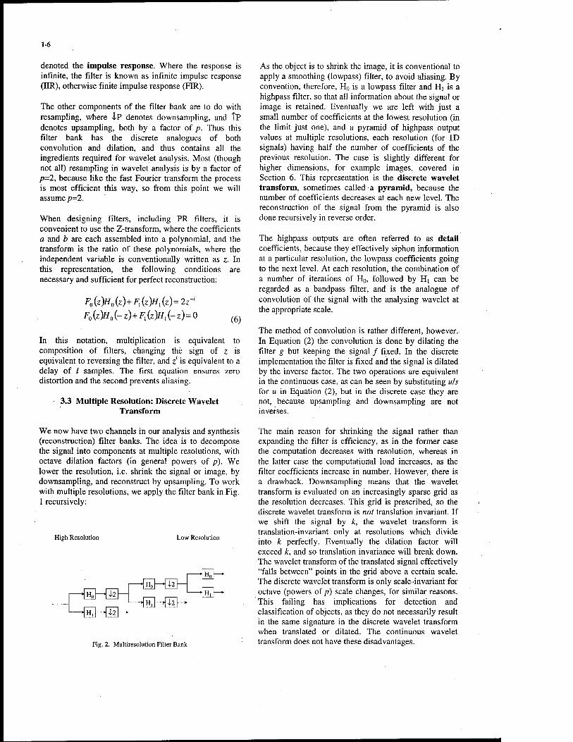
The other components of the filter bank are to do with resampling, where 4P denotes downsampling, and TP denotes upsampling, both by a factor of p. Thus this filter bank has the discrete analogues of both convolution and dilation, and thus contains all the ingredients required for wavelet analysis. Most (though not all) resampling in wavelet analysis is by a factor of p-2, because like the fast Fourier transform the process is most efficient this way, so from this point we will assume p=2.

When designing filters, including PR filters, it is convenient to use the Z-transform, where the coefficients a and b are each assembled into a polynomial, and the transform is the ratio of these polynomials, where the independent variable is conventionally written as z. In this representation, the following conditions are necessary and sufficient for perfect reconstruction:

F0(z)Htt(z)+F](z)H1(z)=2z-1

F{)(z)H0(-z)+Fl(z)Hl(-z)=0 (6)

In this notation, multiplication is equivalent to composition of filters, changing the sign of z is equivalent to reversing the filter, and zl is equivalent to a delay of / samples. The first equation ensures zero distortion and the second prevents aliasing.

3.3 Multiple Resolution: Discrete Wavelet Transform

As the object is to shrink the image, it is conventional to apply a smoothing (lowpass) filter, to avoid aliasing. By convention, therefore, H() is a lowpass filter and Hi is a highpass filter, so that all information about the signal or image is retained. Eventually we are left with just a small number of coefficients at the lowest resolution (in the limit just one), and a pyramid of highpass output values at multiple resolutions, each resolution (for ID signals) having half the number of coefficients of the previous resolution. The case is slightly different for higher dimensions, for example images, covered in Section 6. This representation is the discrete wavelet transform, sometimes called a pyramid, because the number of coefficients decreases at each new level. The reconstruction of the signal from the pyramid is also done recursively in reverse order.

The highpass outputs are often referred to as detail coefficients, because they effectively siphon information at a particular resolution, the lowpass coefficients going to the next level. At each resolution, the combination of a number of iterations of H0, followed by H] can be regarded as a bandpass filter, and is the analogue of convolution of the signal with the analysing wavelet at the appropriate scale.

The method of convolution is rather different, however. In Equation (2) the convolution is done by dilating the filter g but keeping the signal / fixed. In the discrete implementation the filter is fixed and the signal is dilated by the inverse factor. The two operations are equivalent in the continuous case, as can be seen by substituting uls for u in Equation (2), but in the discrete case they are not, because upsampling and downsampling are not inverses.

We now have two channels in our analysis and synthesis (reconstruction) filter banks. The idea is to decompose the signal into components at multiple resolutions, with octave dilation factors (in general powers of p). We lower the resolution, i.e. shrink the signal or image, by downsampling, and reconstruct by upsampling. To work with multiple resolutions, we apply the filter bank in Fig. 1 recursively:

High Resolution Low Resolution

Fig. 2. Multiresolution Filter Bank

The main reason for shrinking the signal rather than expanding the filter is efficiency, as in the former case the computation decreases with resolution, whereas in the latter case the computational load increases, as the filter coefficients increase in number. However, there is a drawback. Downsampling means that the wavelet transform is evaluated on an increasingly sparse grid as the resolution decreases. This grid is prescribed, so the discrete wavelet transform is not translation invariant. If we shift the signal by k, the wavelet transform is translation-invariant only at resolutions which divide into k perfectly. Eventually the dilation factor will exceed k, and so translation invariance will break down. The wavelet transform of the translated signal effectively "falls between" points in the grid above a certain scale. The discrete wavelet transform is only scale-invariant for octave (powers of p) scale changes, for similar reasons. This failing has implications for detection and classification of objects, as they do not necessarily result in the same signature in the discrete wavelet transform when translated or dilated. The continuous wavelet transform does not have these disadvantages.

1-7

4. The Dilation and Wavelet Equations

4.1 Wavelets and Filter Banks

The multiresolution filter bank of Fig. 2 is essentially how the discrete wavelet transform is implemented, but the relationship with the continuous wavelet transform is rather loose, based on the analogue between dilation and resampling. Under certain conditions however, described in this section, there is a much stronger link between wavelets and filter banks, discovered by Stephane Mallat, summarised next. It is based on a construction which allows continuous wavelet transform coefficients to be computed using multiresolution filter banks. This is done using two equations: the dilation equation:

k

and the wavelet equation:

w(jc)=X2A,(*>(2jt-*)

(7)

(8)

where h0 and hi are the impulse response coefficients of the filters H0 and Hj respectively (the equivalent of the coefficients b in Equation (5) if the coefficients a are all zero). <j> is called the scaling function and w is the analysing wavelet which has the same role as g in Equation (2). When convolved with the signal, <j> acts as a lowpass filter (in much the same way as the discrete filter H0) and w is a bandpass filter (analogous to HO- Equations (7) and (8) allow the wavelet transform at one scale to be calculated from the same transform at half this scale, without direct convolution, using the discrete filters Ho and H). To see how this works, substitute <p and w for g in equation (2) to produce two functions wQ(x,s) and W)(x,s), and then sample these functions on a discrete grid with octave scales and position spacing proportional to scale (pyramid sampling):

a(p,q)=w0(2",p) .

b{p,q)=wX2\p) ' p, q integers

We then have the following recurrence relations for a and b:

a(p,q)=YJ^ha(k-2pXk,q + l) k

b{p,q)=Jj^h1(k-2p)i(l,q + l) (10)

which is identical to using the coefficients a(p,q) as input data into the filter bank of Fig. 1 to produce a(p,q+\) and b{p,q+\) as outputs. The multiresolution filter bank of Fig. 2 will therefore produce the values of the wavelet transform function W\ on the pyramid grid, but much more efficiently than by direct convolution.

The filter bank in Fig. 2 works because the scaling function and analysing wavelet are carefully designed so that these functions can be dilated by translation, scalar multiplication and summation, using equations (7) and (8). This is a delicate process, as we require linear combinations of the function <j) and a number of translated replicas to combine to produce the same profile, but dilated. It is a bit like a self-similar jigsaw puzzle: the jigsaw pieces at one scale have to fit together perfectly to produce the same jigsaw piece doubled in size.

4.2 Haar Wavelets

We demonstrate the use of the scaling and wavelet equations with the Haar scaling function and wavelet, which until the 1980's was the only example of a function of compact support known to solve these equations. We begin with the very crude lowpass and highpass filters H0 = [1/2,1/2] and H, = [1/2,-1/2]. We now have the following dilation and wavelet equations:

<t>{x)=<j)(lx)+<t>(?.x-\) w(x)=(t>(2x)-<t>(2x-l) (ID

(9)

which have the Haar scaling function and wavelet as solutions, shown in Table 3.

In this simple case it is obvious how the Haar scaling function (top hat) solves the dilation equation, as the

Table 3. Haar scaling function and wavelet

Name Function Shape Haar scaling function , . (1 0<x<l

[0 otherwise

Haar wavelet

*(*)=•

1 Q<x<\

-1 ±<x<\

0 otherwise

1-8

summands on the right hand side do not overlap, but the existence of other, less trivial solutions (with different filters H0 and Hi) which are smooth and do overlap is much more interesting and useful. The Haar wavelet has some good properties; it is very compact, has a very simple two-point filter and its pyramid translations and dilations form an orthogonal basis. It is not smooth, however, and thus has very poor localisation of Fourier frequency. A major advance was made in the mid 1980's by Ingrid Daubechies, who discovered a family of smooth wavelets which also solve the dilation and wavelet equations. These are now widely used in signal and image compression.

4.3 Existence and Construction of Wavelets

The obvious remaining issue is knowing when there are solutions to the dilation and wavelet equations, are how to find them. Existence and uniqueness depend on the following Toeplitz matrix:

T(H0) =

(Ao(l) h0(2) Äo(3) ha(4)

h0(\) hQ{2) fc(1(3)

h0(l) hB(2)

*b(0

(12)

derived from the lowpass filter H0. We derive another matrix, called the transition matrix:

T0=2T((l2)H0)r(Ha) (13)

The dilation and wavelet equations have a unique solution if the eigenvalues of the transition matrix are less than unity, except for a single eigenvector with unit eigenvalue. Moreover, when this happens we have a simple recursive recipe for calculating the scaling function (j>; it is the limit of the following convergent sequences of functions:

&+,to=I>»(*k(2*-*) (14)

whose resemblance to the dilation equation (7) is obvious. The wavelet function can be derived directly from the scaling function using equation (8).

To summarise, we have achieved a huge gain in efficiency by calculating the wavelet transform using a discrete multiresolution filter bank, but at a price, as we have imposed a constraint on the wavelet function w in the form of the dilation and wavelet equations. For many applications the shape of the wavelet is not critical, as long as it has the required compactness in space or frequency, but there are some applications, for example target detection, where the shape is more important. We have also constrained the evaluation of the wavelet

transform to a discrete pyramid grid, which is also be unsuitable for applications where translation and scale invariance are important.

5. Wavelet Varieties

As with filter design, there are various, sometimes conflicting requirements of wavelet analysis, so there are different types of wavelets which are suitable for different applications, discussed in this section.

Although the scaling and wavelet functions are uniquely determined by Equations (7) and (8), they can still be controlled by the coefficients of the filter H0. The typical approach to wavelet design, therefore, is to design this filter first, along with Hi. The reconstruction filter is then derived from the perfect reconstruction equations (6), which provides the inverse to the discrete wavelet transform. In this section we review briefly some of the many varieties of wavelets and filter banks that are available for ID signal analysis. Higher-dimensional signals, including images, are considered in Section 6.

5.1 Orthonormal Wavelets

The most well known type of wavelet are the orthonormal wavelets discovered by Ingrid Daubechies. Here the filter H() is designed such that the analysing wavelet and all its translations and dilations on the pyramid grid are mutually orthogonal and have unit energy:

jw^.'x + k\>^"x+ p}lx = k = p,l = q

otherwise k,l,p,q integers

(15)

Orthonormal functions are liked by mathematicians because transforms which use these functions are very stable, and trivial to invert, so reconstruction of the signal or image is very easy and efficient. In the case of the wavelet transform the inverse is given by:

/(•*)= JJb(P,q)w{2" x+ p)+Jja(p,g0)w(2'h x + p) p.q«io P

(16)

so the wavelet coefficients on the pyramid are the weighting factors required to reconstruct the signal or image /. A necessary and sufficient condition for orthonormal wavelets is that the filter H0 is double-shift orthogonal, which means that when convolved with its transpose, all the even coefficients are zero except at zero, where the coefficient is two. The odd coefficients do not affect orthogonality of the wavelets. In the Fourier domain these filters are known as half-band, because the power spectrum added to a mirror image about half the Nyquist adds to unity at all frequencies:

1-9

\H(O)] +#(fl) + jrl =1 (17)

The highpass filter Hi is thus derived from H0 by changing the signs of the odd coefficients and then transposing. The synthesis part of the filter bank is identical to the analysis part except for a transpose: h0(k) = f0(-k)andh1(k) = f,(-k).

The remaining task is to design the coefficients of H0 to satisfy Equation (17). This is a complicated process, so only an outline of one method to derive orthogonal wavelets will be given here. First a power spectrum

\H(CO} is found satisfying Equation (17), which for FIR

filters means finding a finite symmetric polynomial satisfying:

P(x)+P(l-x)=l (18)

but where for smooth, band-limited wavelets it is also desirable to have P and as many derivatives as possible zero at JC=0 and x=l, except P(0)=1. The family of solutions, called maxflat filters, is given by:

p^-*y%p+krl\ (19)

Next the coefficients of H0 are derived from P; P is the autocorrelation of H0:

P(z)=H0(z)H0(Z-1) (20)

and solving this equation is known as spectral factorisation. One method is to find all the complex roots of P, which because it is real and symmetric, has roots which come in pairs which are mutually reciprocal. The polynomial H0 is derived by gathering together one root from each pair whose modulus is less than or equal to unity. Fig. 3 shows the Daubechies' wavelets with p-5 and p=&, which become smoother and more band- limited with higher p.

Fig. 3. Daubechies' wavelets DB5 and DB8

7 8 9

(b) p=8

Orthonormal wavelets and filter banks are very convenient, but the constraint imposed by Equation (17) is very restrictive. For example, except for the trivial case of the Haar scaling function, none of the scaling functions, wavelets or filters are symmetrical. It is tempting to use orthogonal wavelets because of their simple inversion formula, but in many cases this is unnecessary, as we often do not require the same coefficients for the analysis and synthesis filters. An analogue is the use of matrices to solve simultaneous linear equations. A matrix with a simple, sparse inverse permits us to solve simultaneous equations easily, but efficient inversion does not require the additional constraint of the inverse being equal to the transpose, as required of orthogonal matrices.

5.2 Biorthogonal and Semi-orthogonal Wavelets

Orthonormal wavelets are the analogue of orthogonal matrices. Likewise biorthogonal wavelets are the analogue of invertible matrices. The inverse of the filter bank is perfect reconstruction, so we still require Equations (6) to be solved, but now the synthesis filters F0 and Fj can be very different to the analysis filters H0

and H|. We also have to work with two types of scaling and wavelet function: one pair for analysis, to calculate the wavelet coefficients using Equation (2), and a different pair for synthesis, to reconstruct the signal or image, using Equation (16). The wavelets and filter banks are still related by the dilation and wavelet equations (7,8), but now the analysis functions are generated by the analysis filters H0 and Hlt and the synthesis wavelets are generated by the synthesis filters F0 and Fj. The perfect reconstruction equations (6) ensure that these wavelets are biorthogonal, which means that in Equation (15) one of the wavelets in the integrand is an analysis wavelet, and the other is a synthesis wavelet, but otherwise the formula is the same.

Semi-orthogonal wavelets are another important variety, where wavelets of different scales are orthogonal, but wavelets of different position are not always orthogonal. These are useful for interpolation and approximation of functions. A popular a simple choice are the spline wavelets, whose scaling functions

1-10

are the Haar scaling function (top hat) convolved with itself n times, and whose lowpass filter has binomial coefficients. The orthogonality across scale ensures that the accuracy of approximation for smooth functions increases with maximum rapidity as scale decreases, but orthogonality between wavelets of the same scale imposes undesirable constraints which degrade approximation

A useful tool which has gained a lot of attention recently is lifting, which is a systematic and flexible method of constructing biorthogonal wavelets and filter banks. The idea is to change H0 to meet application-specific design requirements, whilst still satisfying the perfect reconstruction of Equation (6). It turns out that any change to H0 of the following form will achieve this:

HB(z)^H0(z)+F0(-z)s{z2) (21)

for any filter S(z). We can do a similar operation on the synthesis filter F0, which is called dual lifting. Typically the process of filter design starts with a simple filter, for example a delta function or top hat, called a "Lazy filter", and then the processes of lifting and dual lifting are iterated with suitable choices of S, until the design requirements are met.

5.3 Wavelet Frames

Lastly, we briefly mention wavelet frames. The discrete wavelet transform and filter banks mentioned so far are fully invertible transforms, so there is a one-to-one correspondence between the signal and the output of the wavelet transform or filter bank. This is equivalent to the translations and dilations of the mother wavelet on the pyramid grid being a basis; they are linearly independent and span the space of signals. In wavelet frames the requirement for independence is dropped, which typically involves oversampling the continuous wavelet transform by adding extra points to the pyramid, for example by doubling the resolution in position or by halving scales between octaves. The wavelets still span the signal space, so any signal can be recovered from the wavelet transform. Not all such functions of position and scale are wavelet transforms, however, so wavelet frame transforms only have one-sided inverses.

Wavelet frames are generally more computationally intensive, as there are additional coefficients to calculate, but objects such as targets can be characterised more flexibly at intermediate positions and scales. Wavelet frames become more translation-invariant as the sampling density increases, as they are better approximations to the continuous wavelet transform.

To summarise, there is a wide variety of wavelets and filter banks available for signal analysis, each with its own strengths and weaknesses. Although it is tempting to use the first family of wavelets that springs to mind,

for example the popular Daubechies wavelets, there may be others more suitable for the application. There are also design techniques, such as lifting, to customise wavelets, should off-the-shelf varieties not suffice.

6. Wavelet Analysis in Higher Dimensions

The techniques described in Sections 3-5 are applicable to 1-dimensional signals. In higher dimensions there are two approaches to wavelet analysis: either to use separable filters which can be derived easily from ID filters using exterior products, or non-separable filters, which have to be designed from scratch, which is more difficult.

6.1 Separable Wavelets

Separable functions of several variables are Cartesian products of functions of fewer variables:

f(xl,x2,...,xn)=fl(xl)f2(x2)...f,Xx„) (22)

where in general the arguments xk can be vectors as well as scalars. Exterior products of scaling functions and wavelets make effective higher-dimensional wavelets, inheriting all the properties of their lower-dimensional components. To simplify the notation, we will consider exterior products of two 1-dimensional wavelets to facilitate image wavelet analysis, but the principles behind higher-dimensional wavelet analysis are identical.

Image wavelet analysis involves one lowpass filter H0

and three highpass filters, Hi, H2, H3, each of which is the exterior product of 1-dimensional lowpass or highpass filters:

h0(m,n)= ha(m\{n) hl(m,n)=h0(m)h1(n) ^3)

h2(m,n)=hl{m)ha(n) h3(m,n)= ^(mfain)

Similarly there is one scaling function and three wavelet functions formed as exterior products of their 1- dimensional counterparts:

</>2(x,y)=w(x)t>(y) <p3(x,y)=w(x)w(y) (24)

The multiresolution filter bank has four outputs at each scale; the lowpass output is downsampled and goes to the next resolution, and the other 3 outputs are the detail or wavelet coefficients, as for the 1-dimensional case. The three types of wavelet are usually regarded as having horizontal, vertical and diagonal orientation.

The discrete wavelet transform is usually displayed as shown in Fig. 4, though this representation can be misleading. In this representation the density of wavelet

1-11

coefficients is kept constant, with larger regions required to store information at high resolution (low scale). The wavelet coefficients at any scale are three times the number at all larger scales, because there are three highpass filters to one lowpass filter. The regions are designated LL (lowest resolution only) HL, LH and HH according to Which combination of 1-dimensional filters is used in the Cartesian product. This representation is convenient, because the transform has the same shape and number of pixels as the original image, an example shown in Fig. 5, but the larger scales are portrayed as being smaller in size! It is true that the downsampling operator has this effect, but a more natural interpretation is that the wavelet filters increase in scale.

LH HH

LH HH

HL LH HH

HL LL HL

Fig. 4. Image wavelet display

m & ■

, %%&L ........... ...,

yard pi V^S? fky :;%:%??:•" i

t '^MWM'nWti'V'ySf^^-\-'' «--:'•:;•> ;■■ ->^' !

-Z ■«*«/•->iE • w-r.■I*«JII*L« • ' • mmmmmm

Fig. 5. Wavelet decomposition of 'Lena' - 2 levels

6.2 Non-Separable Wavelets

The alternative approach to image wavelet analysis is to use non-separable wavelets. Although more difficult to design, these can be more flexible, especially in orientation. The image pyramid grids and resampling do not need to be rectangular or separable, either. An example is given in Fig. 6, where the small and large dots comprise the grid at one resolution, and the large dots only comprise a sub-grid at the next lowest resolution.

• •

I •

• I

Fig. 6. Non-separable grid

In this example the change in area and the resampling factor between scales is not 4 as it would be in the separable case, but 2, so there is only one highpass filter required, as for the 1-dimensional signal case. In this case resampling causes a rotation through 45°. This is known as quincunx resampling. Hexagonal grids can also be used, which permits wavelets with 60° orientation intervals to be constructed. Even more exotic wavelet grids have become popular in the interpolation of complex geometric surfaces [7], which is a very active research topic.

7. Wavelet Packets

In conventional wavelet analysis the main source of variety in the transform is in translation and dilation. One or a very small number of filters is involved, except for differences in position and scale. This limits the variety of information that individual wavelet coefficients represent. Another approach that has gained popularity in recent years is that of wavelet packets, where the functions used to represent the signal or image vary in shape also. Typically frames are used instead of bases, initially providing redundancy, but then a subset of the coefficients are selected to derive a basis which is adapted to fit the incoming data.

One way to do this is the extend the sub-band coding to encompass any dyadic tree structure. In conventional wavelet analysis it is only the lowpass filter that is split further by downsampling and bandpass filtering; the

1-12

output from the highpass filter is left alone. In a more general dyadic tree, the decision to split the channel is applied more arbitrarily, to yield a wide variety of transforms. Fig. 7 shows some examples of dyadic trees.

Lowpass

r£

HI 4:

Highpass

Wavelet tree Complete tree Wavelet

packet tree

Fig. 7. Dyadic tree structures

The complete dyadic tree divides all branches, resulting in an equal partition in the Fourier domain, analogous to the short-time Fourier transform which divides the signal into a set of time-frequency cells of identical duration and frequency bandwidth. If we apply the complete tree to the Haar filter, for example, we get the Walsh functions, shown in Fig. 8.

Fig. 8. Walsh functions

In general the aim of wavelet packet analysis is to approximate the signal or image by a series of functions chosen from a large set, called a dictionary, for example the functions generated by all dyadic trees. The functions are chosen to give the best approximation with the smallest number of components. The larger the dictionary, the more computation required, but also the greater the potential for an efficient representation. An alternative approach is to extend the transformations which generate the wavelet basis beyond translation and dilation to include shape changes, for example frequency shifts and chirp angles (chirplets [8]), or in the case of image wavelets, affine transformations (ridgelets [9]).

There are also different approaches to choosing the functions from the dictionary to approximate the signal or image. One method is the best basis algorithm [10] which selects functions from a union of several bases. Another is matching pursuit [11], where wavelets are

selected from a large dictionary (e.g. generated by translation, dilation and frequency shifts) in the order that most rapidly decreases the approximation error, and at each stage subtracts the chosen function from the signal or image. Another method [12] is selection from a continuum of functions analogous to the continuous wavelet transform, searching for local maxima in correlation with the signal or image, but where parameters are not limited to position and scale, or to a discrete grid. A conjugate gradient search is used to refine the wavelet parameters after an initial grid search, enabling the wavelets to fit the signal or image data more accurately, and achieving invariance with respect to translation, dilation and related operations.

9. References

1. G. Strang and T. Nguyen, Wavelets and Filter Banks, Wellesley-Cambridge Press, Rev. Ed., 1997.

2. Y. Meyer, Wavelets, Algorithms and Applications, Siam, Philadelphia, 1993.

3. Feder J., Fractals, Plenum Press, 1988.

4. A.K.Jain, "Image Data Compression: A Review", Proc. IEEE, 69, pp.349-389, 1981.

5. T.H. Koornwinder (ed), Wavelets: An Elementary Treatment of Theory and Applications, World Scientific, 1993.

6. G.H.Watson, "The Detection of Unusual Events in Cluttered Natural Backgrounds", NATO RTA lecture series 216, Application of Mathematical Signal Processing Techniques to Mission Systems, 1999.

7. A.W.F.Lee et al, "MAPS: Multiresolution Adaptive Parameterisation of Surfaces", Computer Graphics Proceedings (SIGGRAPH 98), pp.95-104,1998.

8. S.Mann and S.Haykin, "The Chirplet Transform: Physical Considerations", IEEE Trans, on Signal Processing, 43(11), Nov 1995.

9. EJ.Candes, "Ridgelets: Theory and Applications", PhD Thesis, Dept of Statistics, Stamford University, 1998.

10. R.R.Coifman and M.V.Wickerhauser, "Entropy- Based Algorithms for Best Basis Selection", IEEE Trans, on Information Theory, 38, pp.713-8, 1992.

11. S.G.Mallat, "A Theory of Multi-Resolution Signal Decomposition: Wavelet Decomposition", IEEE PAML, Vol. 1, pp. 674-693, 1989.

12. G.H.Watson and K.Gilholm, "Signal and image feature extraction from local maxima of generalised correlation", Pattern Recognition 31(11) pp.1733- 1745, Nov 1998.

© British Crown copyright 1999. Published with the permission of the Defence Evaluation and Research Agency on behalf of the Controller of HMSO.

2-1

The Detection of Unusual Events in Cluttered Natural Backgrounds

G.H.Watson


1. Introduction

This paper is concerned with the use of wavelet analysis and statistical models of natural backgrounds as a means of detecting unusual events within, in particular targets of military interest. The underlying principle is to detect targets as objects that stand out from the background, and hence are unusual, rather than searching for objects with prescribed characteristics and dealing with clutter as an afterthought. First a method of feature extraction is described based on wavelet analysis which is used to characterise both backgrounds and unusual events. Then the statistics of these features for natural backgrounds are considered, making use of fractal geometry, from which basic clutter rejection can be implemented. More advanced clutter rejection methods are then considered, based on the multivariate statistics of additional measurements. Three cases are considered in detail: the wavelet analysis of multispectral data, the use of local variance to reject clutter in intermittent backgrounds, and the use of temporal variability to reject clutter in image sequences.

The approach of modelling the background, rather than the target, has the advantage that little or no prior knowledge of the latter is required, leading to greater flexibility and robustness. Target prior can be added at a later stage, if available, for further discrimination and clutter rejection. In some military circumstances early warning of targets is required before any detailed structure can be resolved, the limiting case being point targets with a single-pixel signature. In such cases target prior is of little use in recognition, being limited to the time signature of a single pixel, so the use of background context can be critical to early detection.

The method to be described comprises the following stages:

(a) Decompose the signal or image data into a set of discrete features which are suitable as an ensemble for characterising both targets and the background. These features are generally simple geometric shapes to facilitate their extraction, such as blobs and bars in images, but which can be combined to characterise more complex objects, such as roads and cloud edges. These features are usually extracted at multiple scales, using wavelet analysis.

(b) Construct a statistical model of the background based on the above feature decomposition. Most natural backgrounds are difficult to model, having strongly non-Gaussian statistics and phase correlation, for example in the form of strong edges. In general the joint statistics of feature parameters such as brightness, position, scale and orientation need to be calibrated, resulting in multidimensional probability distributions. However, most natural backgrounds are stationary and exhibit fractal geometry, which simplifies the statistical modelling.

(c) Extract potential targets as statistical outliers, that is at the edges or tails of the background distribution. Each object is assigned a prior probability that it belongs to the background, and hence not a target.

(d) If additional target prior is available, use Bayes' formula to combine the prior distributions of targets and the background to estimate the a posteriori probability (likelihood) of there being a target. This topic is not covered in this paper.

This method can be applied to a wide variety of data, including 1-dimensional signals (e.g. acoustic data), 2- dimensional images (including multispectral imagery), 3- dimensional images (e.g. medical tomography), and time-sequenced imagery, where movement is part of the feature characterisation. The method is only limited by the methods of feature extraction available, and the accuracy of the background statistical models.

The remainder of this paper is organised as follows. Section 2 describes methods of feature extraction, based on searching for local extrema in the wavelet transform and analogous correlation, and explains the relationship between this and matched filtering. Section 3 describes how the statistics of these wavelet features are calibrated with the aid of fractal geometry. Section 4 explains how improved clutter rejection can be implemented by introducing additional random variables, and gives three examples: multispectral imagery, strongly intermittent backgrounds, and image sequence clutter rejection based on space-time filters.

2. Feature Extraction

As explained in Section 1, the purpose of feature extraction is to decompose the signal or image into a set



2-2

of discrete geometric components which are sufficient to characterise both targets and background sufficiently well that the former can be recognised as unusual events. This involves making measurements of the data for which targets might have unusual values, which in signal processing parlance means applying filters to the data. The most well understood filters are linear, which will be considered in this section; Sections 4.2 and 4.3 give examples of non-linear filters which provide further discrimination of targets and clutter.

2.1 Features from Matched Filters

Matched filter theory [1,2] can be used to derive the optimum linear filter (matched filter) to detect any prescribed object, in the sense that signal to noise ratio (SNR) is maximised. If/ is the filter, x is the target then SNR is defined to be:

\m W»f)

(i)

where E denotes expectation. In this section it will also be assumed that the signal or image data is stationary, that is statistically translation-invariant. This is usually the case for time-varying signals and imagery projected as a plan view, but there is often a statistical dependence on the vertical image co-ordinate for forward-looking imagery. The latter situation is considered in Section 4.3. For translation-invariant data the filters should be translation-invariant to avoid statistical bias, which implies linear filtering is equivalent to convolution. In such cases the Fourier transform of the matched filter F((o) is given by:

F(co)-- N(co)

(2)

where X is the Fourier transform of the target, the bar denotes complex conjugation, and N is the power spectral density (PSD) of the background. The inverse Fourier transform can be used to derive the convolution kernel in the signal or image space.

Matched filters are simple and effective when the target configuration is simple, for example a point target, as the number of possible target configurations may be small. Where the target is more complex, either because spatial structure can be resolved or because its trajectory is varied, the number or complexity of matched filters makes their implementation more difficult. For example, an aircraft may be viewed from many ranges and aspects, each requiring a different matched filter. In this paper matched filters are designed instead to detect simple geometric structures which are suitable for characterising parts of targets or backgrounds. For example, if the target is a missile, we may choose a bar shaped

component; this will not fit the missile exactly, but gives a fairly good approximation to the missile body and the plume. If we choose very simple, generic components, we will be able to pick up a wide variety of objects, but there will be some loss in detection sensitivity when the SNR is very low.

2.2 Translation and Dilation Invariance

Convolution involves correlating the kernel with the data and repeating this operation over all translations of the kernel. Translation is usually required because there is little or no knowledge of where the target is located in space or time prior to its detection. It is fortunate that many backgrounds are also statistically translation- invariant, otherwise translation of the filter kernel would not give consistent answers. Non-stationary backgrounds, such as in forward-looking imagery are a common source of false alarms for this reason.

In many situations the scale of the target signature is also not known a priori, primarily because it is affected by the distance to the sensor. Thus multiresolution analysis is required, where the filtering is repeated over varying scale as well as varying position. This is why wavelet analysis is a useful tool in target recognition. Even when there is prior knowledge of target size, the geometric features used in its analysis may be of varying scale, for example a missile's guidance fins are usually much smaller than its fuselage.

Many backgrounds are statistically scale-invariant, though this is not as intuitively obvious as translation- invariance. In many images of familiar scenes, such as natural terrain, the scale or magnification is hard to discern unless there is a reference object of known size, such as an adult human. This phenomenon is the subject of fractal geometry [3,4], where scale-invariance is known as self-similarity. Strictly speaking self-similarity means that there is a scaling transformation under which the signal of image is identical to a subset of itself, where the scaling transformation is given by:

W fix) (3)

where/is the signal or image being transformed, s is the scale or dilation factor and the constant h is sometimes called the self-similarity parameter. When modelling natural backgrounds the equality of equation (3) is replaced by statistical invariance. The response of statistically self-similar backgrounds to filters at different scales can be normalised by dividing by sh [5], allowing the same threshold to result in the same false alarm rate over a range of scales. We will return to the use of fractal geometry in modelling the statistics of backgrounds in Section 3.

2-3

2.3 The Wavelet Transform

So far we have established that correlation should be combined with translation and dilation, resulting in wavelet analysis, and that the background is often translation and scale invariant, which means that the statistics of the wavelet transform should be uniform. However, care must be taken to employ the correct scale normalisation factor s'h, to ensure uniformity. The standard definition of the continuous wavelet transform is consistent with h=-Vi, the self-similarity parameter for uncorrelated backgrounds (white noise):

T(p,s) = s []f(x)g 'x-p^

dx (4)

but in general, for constant false alarm rate (CFAR) detection, the formula should be modified to:

T(p,s) = s-i-h]f(x)g 'x-p^

dx (5)

The shape of the analysing wavelet g can be derived as the matched filter of the geometric feature which will be used to characterise the signal or image data, at a chosen position and scale. If more than one type of feature is used, for example radial basis functions and oriented bars, then more than one analysing wavelet is required, and more than one wavelet transform calculated.

The use of matched filter theory to derive appropriate analysing wavelets shows that the latter depend on both the shape of the geometric features used to characterise the data, and on the properties of the background, in particular its PSD. For uncorrelated backgrounds the matched filter is the same as the geometric feature, except for a reversal in space and time (a mirror image). For most correlated backgrounds the PSD decreases with frequency, so the matched filter is similar to the feature, except higher frequencies are emphasised, which has the effect of introducing side-lobes. For self-similar backgrounds the PSD is a (usually negative) power of frequency [5], and the matched filter is thus a fractional derivative [6] of the feature. For example, in Brownian noise the matched filter is the time-reversed second derivative of the feature, and the equivalent operator for rotationally-symmetric image backgrounds is the Laplacian operator. In the latter case the matched filter for a Gaussian radial basis function is its second derivative, which is similar to the Difference of Gaussian (DoG) filter so popular in target detection.

2.4 Local Maxima

The final stage in feature extraction is searching for local maxima in the absolute value of the wavelet transform, as this enables the data to be decomposed into a discrete set of objects, and reduces redundancy. Restricting

measurements to local maxima, rather than at all points above a threshold, prevents redundant features being generated from the same object in its neighbourhood. At each local maximum, its location in wavelet space (position and scale), and the type of analysing wavelet (e.g. matched to a blob or bar) are recorded, as well as the wavelet transform value itself. These values provide a lot of information about targets and backgrounds, for example the location, scale, orientation and grey-level contrast of edges and bars, and an approximate reconstruction is available by linear superposition of the features whose parameters match the local maxima. In the context of target detection, it is more useful to retain only those features whose amplitude (wavelet transform value) exceed a threshold corresponding to a prescribed probability (Section 3). These features provide concise information about the target and effective clutter rejection, from which a partial reconstruction of the target can be obtained. Examples of feature extraction and partial reconstruction are given in Fig. 1, demonstrating the ability to represent artefacts such as roads and buildings, whilst rejecting most clutter.

The method of searching for local maxima depends on the application. A search restricted to the positions and scales of the discrete wavelet transform is quick to implement, but the resulting features are limited by the poor resolution of the pyramid grid of positions and scales. This type of feature extraction is also not truly translation and scale invariant, because most shifts in position and scale cause the wavelet grid to change. This drawback is mitigated if a wavelet frame is used with a higher resolution in position and scale, which is equivalent to interpolating the wavelet transform. Better still, but more costly, is to refine the positions and scales of the features thus found by evaluating the continuous wavelet transform explicitly using expanded filters instead of downsampling the signal or image, and then optimising this function using a local search, for example a conjugate gradient search [7]. This method results in true translation and scale invariance.

3. Background Statistics and Fractal Geometry

3.1 Threshold Exceedance Model

Once geometric features have been extracted from the data (Section 2), the next stage is to discriminate between potential targets and the background, based on the statistics of the latter. First we describe a simple statistical model for backgrounds with fractal geometry which predicts the rate at which feature amplitude (wavelet transform value) exceeds any prescribed threshold y as a function of scale s. Jones [8,9,10] has shown that amplitude threshold exceedance rates are proportional to a power of scale, s'D, where D is a fractal dimension describing the self-similarity of feature

2-4

population, which is different to h (Section 2), describing the self-similarity of feature amplitude. This self- similarity enables a single scale-independent distribution to represent the joint statistics of amplitude and scale:

NysD=F(y) (6)

where A^ is the threshold exceedance rate (number of features whose amplitude exceeds the threshold y), and F is a scale-independent function defining the shape of the distribution.

whereas c=2 represents a Gaussian distribution with weak tails.

Equation (7) can be used to assign an a priori probability that a geometric feature arises from the background, and by setting a threshold on this probability, driven by the highest acceptable false alarm rate, the detection of targets as unusual events is possible. For backgrounds with translation and rotation invariance, we thus have a simple method of target detection with no bias in position, scale or orientation.

The threshold exceedance statistics in [8] and for the data analysed in this paper are approximated well by the generalised exponential function F(y) = yc/ß where c and ß are constants. This leads to the following model for threshold exceedance statistics:

where:

log f \T „D\ ( \ Nys

L

a \ J V

(7)

• N is the number of local extrema at scale s whose amplitude T(p,s) exceeds the threshold value v. N as a function of y is closely related to the cumulative probability distribution of wavelet amplitude T at the local extrema.

• D is a fractal dimension, and represents the scaling behaviour of the population density of local extrema with respect to position. For statistically stationary signals the fractal dimension is equal to the topological dimension, that is 1 for signals, 2 for images and 3 for image sequences or tomography. For intermittent self-similar data the fractal dimension can be less than the topological dimension because of the hierarchical clustering of local extrema, where at any scale a cluster is formed of several smaller clusters with intervening gaps. The Cantor set is an example of a ID signal with a fractal dimension of less than unity.

• or is called lacunarity, which is a measure of overall population density of local extrema in a fractal.

• ß is a measure of overall intensity, which in a stationary process would be proportional to the standard deviation of the signal or image.

• c is an inverse measure of the strength of the tails in the distribution of wavelet amplitude. For example c-\ represents an exponential distribution with moderately strong tails,

3.2 Calibration of the Model

To use equation (7) we need to know the values of the parameters D, a, ß, c and the self-similarity parameter h (Section 2). In some cases there is prior knowledge of some or all of these parameters, for example there are theoretical reasons for assuming a self-similarity parameter of h=\ß for fully-developed turbulent flow [11]. More often it is better to estimate these parameters from the signal or image data. This can be done off-line as a separate training process, with the advantage that there will probably be independent assurance that targets are missing from the data. On-line calibration has the advantage that the resulting detection algorithm can adapt to changing background conditions, for example caused by changes to the weather.

We now describe a simple and efficient method of estimating D, a, ß, c and h, making frequent use of linear least-squares regression. The data used in this statistical estimation is assumed to be a set of feature amplitudes and scales (yk, sk). First, an approximate value of self- similarity ha is used to calculate the modified wavelet transform of equation (5). This can be estimated with reasonable accuracy from the slope of the PSD plotted in log-log co-ordinates; in theory the PSD should be proportional to s

<2h+)) [5]. The self-similarity parameter will be refined based on estimation from feature amplitudes and scales. The initial guess only weakly affects the location and density of local extrema in the wavelet transform, so high accuracy is not required.

Next, threshold exceedance counts Ny are derived, conditioned by scale, for a range of scales s and amplitudes y. The conditioning of scale depends on the method of searching for local extrema in the wavelet transform. If the search is limited to values of scale on a discrete grid, then these values are used to partition the data, and threshold exceedance counts are computed for each partition set. On the other hand, if scales are refined, for example using a gradient search, it is necessary to partition scales into a set of intervals. Threshold exceedance counts Ny are derived for a range of values y for each scale or scale interval. An efficient way of doing this for every value of y in the geometric feature set is to sort the amplitudes of the latter into

2-5

descending order; the value Ny for each y is then its index in the sorted array.

The next step is to assign a weight to each pair of (y, A^.) which reflects its relative importance when fitting the model given by equation (7). The weights depend on the confidence in the data at the tails of the distribution where y is large and Ny is small. Where we are sure that there are no targets, i.e. the background is "pure", it is appropriate to assign relatively large weights at the tails, as it is the latter which are important in discriminating targets from clutter. In this case assigning weights which have uniform density in amplitude y, or even density which increases with y, is appropriate, which can be done by setting each weight to be the difference between y and the next lowest value of y in the same scale partition. Alternatively, where there may be targets present, for example during on-line calibration, it is better to give the tails low weighting, and rely on the model in equation (7) to extrapolate these. This can be done by assigning equal weights to each pair (y, A^,), as the number of target features is almost always orders of magnitude lower than the number of background features.

The parameters D, a, ß, c and h, are now estimated using linear least-squares regression with the weights described above. First we need to rewrite equation (7) to allow for the difference between the approximate self-similarity parameter h0 and the actual self-similarity h:

log iNys°] = - ( Y

y

a v J

s"-"°ß (8)

The tail strength c is estimated by fitting a linear model to (log(y), log(log(Ay)) and measuring the slope. Next a linear model is fitted to (-yc, \og{Ny)) for each scale partition, as follows:

log(ATy)=A,-B, y (9)

where the slopes and intercepts As and Bs depend on scale s. Then linear models are fitted to the following data: (log(s), As) and (log(s), -log(fi.v)) resulting in:

and

A, =P,+/>2log(j)

-log(B,) = P3+P4logM

Substituting (10) and (11) into (9) we obtain:

( log

A7. -y exp^V2 ' exp(P3)y''4

(10)

(11)

(12)

Comparing equations (8) and (12), the parameters D, or, ß, and h, are derived straightforwardly from the slopes and intercepts Pu P2, P3 and P4.

4. Clutter Rejection from Joint Statistics

For some backgrounds, for example where clutter is intermittent, detection sensitivity can be increased by taking additional measurements into account, thus introducing additional criteria for discriminating targets and the background. In this section we describe a method of doing this based on the modelling of the joint statistics of wavelet amplitude and other variables describing the background.

4.1 Vector Fields

The most straightforward example of additional measurements is the analysis of vector fields rather than scalar data, in which each sample pixel has a vector value. Examples of vector fields are fluid flow velocity, electromagnetic fields, and multispectral imagery. In this case the joint statistics of wavelet amplitudes of each component of the vector (treated as a scalar field) are modelled. These wavelet amplitudes are the components of a multiresolution vector field which is a vector analogue of the wavelet transform:

T(p,s) = s-l-"]f(x)g fx-p^ dx (13)

where correlation now involves pointwise multiplication of the vector field f by the scalar filter g and integration is vector summation. Matched filter theory can still be used to design analysing wavelets, but now the power spectrum contains information about the cross correlation of the vector components at each frequency, as well as their autocorrelation.

There is no direct analogue of the feature extraction of Section 2 for vector fields, because local maxima of the wavelet transform are not defined, being vector valued. If the probability density function (PDF) of the wavelet transform were known a priori and easy to compute, then we could derive a scalar-valued function of the wavelet space by composing the above vector wavelet transform (which maps wavelets to a vector space) with the PDF (which maps the same vector space to the real line). It makes sense to search for local minima in the composite function, as these correspond to locally unusual events. There are two drawbacks to this:

• Joint PDFs are difficult to estimate accurately, with the difficulty increasing rapidly with the number of vector components. Over-fitting the PDF to the training data is a common problem [12].

• Not all outcomes of low PDF correspond to likely targets. For example, when based on local maxima, most distributions of wavelet amplitude have low PDF near the origin, corresponding to very low

2-6

feature brightness or contrast. These features are not usually target related.

In view of the above problems, the usual approach is to search for local maxima of a derived scalar quantity, the Mahalanobis distance [13]:

D(T)=(T-juJC-l(T-ju) (14)

where fi is the vector mean of the wavelet transform values T, and C is the multivariate covariance matrix of T. For Gaussian distributions D is proportional to the negative logarithm of the PDF, and so is an unbiased measure of rarity. This measure is also only high for unusually high wavelet amplitudes (relative to the mean) at the external boundary of the distribution, so ignores very faint features. Like principal component analysis, this method is very effective at extracting features with unusual vector direction as well as amplitude, especially when there is a high level of correlation in vector direction. This situation is common in multispectral imagery when the spectral bands of the background are close in radiation frequency, resulting in a limited range of "colour". Objects which have an unusual radiation spectrum (colour) often generate wavelet amplitudes with a large Mahalanobis distance, even when none of the vector components is unusually large regarded in isolation.

The example in Fig. 2 concerns 5-band AVHRR (Advanced Very High Resolution Radiometer) satellite imagery of sea surface background. This data is a fusion of two visible bands (0.6 and 0.8 |xm) and three infrared bands (3.7, 11 and 12 u.m). The objects of interest are tracks which arise from ship plumes altering the spectral properties of the cloud. These tracks are visible in Band 3 (3.7 |xm), and are generally absent or very faint in the other bands. Figs. 2a and 2b show an example of such a track against cloud clutter in Bands 1 and 3 respectively: the local SNR of the track is greatest in Band 3, but not sufficient to be easily distinguished from the cloud edges, especially towards the top of the picture. We base our analysis on these two bands because the other bands are either very similar in frequency or contain little new information.

Figs. 2c and 2d illustrate the advantage of basing the Mahalanobis distance on the wavelet transform T (Fig. 2c) rather than the raw pixel values (Fig. 2d); the ship track stands out much more clearly in the former case.

4.2 Intermittent Backgrounds

Another example of the use of additional random variables concerns the modelling of strongly intermittent backgrounds, in which some regions are energetic (highly cluttered) and others are relatively quiescent. Statistical translation-invariance does not rule out this

kind of variability with respect to position; it implies only that global statistics are invariant. Local statistics, such as standard deviation over a neighbourhood of the signal or image, may still be position-dependent, and often are for natural backgrounds. Variation in local statistics happens either because the image background comprises more than one texture, for example associated with woodland, mountains and sea, or because a single texture type is spatially intermittent, in which some regions are more energetic than others.

Intermittency is represented implicitly in the statistical model of Section 3 by the fractal dimension D and the lacunarity a, but no account is taken of the dependence of the average amplitude or population density of the geometric features on their position, i.e. their tendency to cluster. Thus whilst the effect of clustering on global population densities is accounted for, the variation in local density with position is not. If position dependence is not modelled, the same thresholds will be applied to energetic and quiescent regions alike, resulting in either a loss of sensitivity in the latter or too many false alarms in the former. We now show how the joint statistics of wavelet amplitude and a non-linear function, local energy, is used to rectify the above limitation. Further detail is given in [14].

The most obvious method of allowing for spatial variations in background activity is to condition the background model given by equation (7) with respect to position. This approach would require statistical distributions to be measured over neighbourhoods of the signal or image and then the model parameters fitted in each case separately. This approach is not effective because the fractal model parameter estimation only works well with large images (at least 64x64 and usually much larger) as filter statistics need to be compiled over a number of scales and in sufficiently large numbers to estimate a cumulative distribution function. The fractal model has the advantage of realism when applied to large images but at the cost of a rapid decrease in accuracy for images much below 128x128 pixels, and is thus unsuitable for the representation of local statistics.

In any model of the background which is conditioned by position, there is an inevitable conflict between the accuracy of the estimation of statistical parameters on the one hand, and spatial resolution of background intensity levels on the other. For the purposes of target detection, good spatial resolution is important because the threat, for example an incoming missile, may be very close to clutter, such as cloud edges, which could lead to incorrect thresholds being used by the detection process. The advantages of measuring background activity levels with spatial resolutions of less than 64 pixels in such cases are obvious. It follows that in the choice of the representation of local statistics, spatial resolution should be given a high priority. To achieve high spatial resolution, local background activity needs to be

2-7

represented by a robust statistic which requires a small amount of image data to compute reasonably accurately. This is why a simple non-linear measure, local energy, has been chosen for the spatial conditioning of the background statistics.

Local energy is a measure of local background activity which is computed over neighbourhoods of varying size surrounding each geometric feature extracted from the data (Section 2). Local energy E(x, L) is defined to be the variance of the signal or image over a region centred on x and of size L. For ID signals this region is a subset of the real line, for example an interval of length L, for 2D images it is a subset of the real plane, for example a square, and for 3D image sequences a subset of space- time. Detection sensitivity is generally improved if the support of the geometric feature is subtracted from this region, so that the wavelet amplitude and local energy are less mutually dependent.

The region size L is defined relative to the scale s of each extracted feature and is not to be confused with the scale of the feature itself. Local energy measurements over variable size L are required to achieve the best balance between spatial resolution and accuracy of local energy measurement. In cases where a potential target is close to but not within an energetic region, a small local energy region gives the best probability of detection. In cases where the background activity is more uniform, however, fainter targets can be detected with greater sensitivity where background levels have been measured over an extended region. The following region sizes L have been considered in this paper: 2, 4, 8, 16 and 32. We now describe how the joint statistics of local energy at each size L and wavelet amplitude T are used to model spatially intermittent backgrounds and improve the discrimination between targets and clutter, illustrating the technique on infrared imagery of the celestial background (Fig. 3) in which some simulated point targets have been inserted.

Fig. 4 shows the joint statistics of T and E in the form of a scatter plot, where L is set to 8, background data are presented by points, and the targets by crosses. The scatter plot resembles the joint PDF of these random variables, as regions of high population density in the scatter plot correspond to regions of high PDF. The embedded targets are mostly separate from the background distribution, that is in a region where the background joint PDF is low. Thus in this case most of the targets can be distinguished from the background as statistical outliers, but they are not outliers with respect to wavelet amplitude alone. Some of the target crosses are located within regions of high background density, but these all have high local energy and thus correspond to targets embedded in strong clutter, in this case IR cirrus, where the targets are very difficult to identify by visual inspection. When in regions of low local energy,

the targets are bright relative to the local background and are thus perceived more easily.

The modelling of the joint distribution of y and E is done along similar lines to the joint distribution of T and 5 in Section 3, to avoid the disadvantages of estimating the joint PDF of more than one random variable mentioned in Section 4.1. Once the self-similarity parameter h has been estimated, y is independent of scale, so the dependence on s can be ignored. Details of the modelling of Tand E are given in [14], an outline of which is given here. The idea is to predict the conditional cumulative probability distribution of T given E. Observation of real and simulated intermittent data (e.g. Fig. 3 for the IR celestial background) has shown that this conditional distribution is self-similar, being only dependent on an energy-dependent dilation factor, which can be estimated by calculating the conditional standard deviation of T as a function of E. It has been found that a power-law fits this function quite well, so the following model of conditional threshold exceedance probability has been used:

Pr(y'>;ylE'=.E) = exp ( y V

I W ) (15)

The parameter r is another measure of intermittency of the background, and can be estimated by linear least squares regression of the logarithm of conditional standard deviation versus the logarithm of local energy. The following energy-normalised wavelet amplitude

I=TE'r (16)

is an energy-independent measure of rarity, and targets and clutter can be discriminated more effectively based on / instead of the un-normalised y. Fig 5 shows the joint statistics of / and E, where it can be seen that the dependence on E is greatly diminished compared with T (Fig. 4), and that a single threshold on / is sufficient to detect most targets with very few false alarms.

The last step is to combine the rarity measures I(L) over multiple regions sizes L. The idea is to select the "best" region size L given the local distribution of clutter. If the object in question is completely embedded in relatively strong clutter then detection will be difficult for any size L. If the object is close to but not embedded in strong clutter then a small L will give the best detection sensitivity, but a larger value is better otherwise. The "best" size corresponds to the largest region not overlapping strong clutter, in which local statistics are most accurately represented.

An overall measure of rarity is therefore defined as follows. First I(L) is normalised by dividing by its standard deviation over all wavelets. Then for each

2-8

feature the largest region size L is selected for which the function l'(L) given by:

l'(Ln) = I(Ln)-I(Ln_1), n>2 (17)

is less than 3.5 for all lower scales:

Lmax = max{L„: l\Lk) < 3.5ö V/t: 2 < k < n} (18)

Sudden decreases in /(L) are considered because these correspond to a step increase in local energy, which occurs when a region of clutter is encountered, as required. Decreases of less than 3.5 standard deviations are ignored on the grounds that they are not strong enough to correspond to large changes in background statistics. An overall measure of unusualness is then defined as the mean value of / of size not exceeding»

'oPl= X/ao/Xi (19)

Maximum and minimum values of /(L) were also investigated but were found to be less robust discriminators between targets and the background.

Figs. 6a and 6b compare the target detection performance of the original scale-normalised wavelet amplitude T and the new energy-normalised measure /, where in both cases the threshold has been set at 2 standard deviations (of Tor /). The use of Tresults in 21 targets being detected along with 19 false alarms, compared with 29 targets and only 1 false alarm when / is used. The improvement in performance is due to the ability to take local background conditions into account in the neighbourhood of each target.

4.3 Image Sequence Analysis: Track Before Detect

The final example of the use of additional random variables is to aid the detection of targets in time- sequenced imagery, where target motion and the evolution of clutter in time need to be taken into account. Many target detection methods, including most earlier ones [15], are based on "track after detect", in which initial processing is limited to single frames, and track association algorithms are employed subsequently to characterise movement. These methods are not effective when there is insufficient information in single frames to discriminate targets from a large number of clutter objects, typically when the target is amongst clutter of equal of greater edge contrast, or of similar texture, such as roads, buildings, cloud edges and sea glint. Human vision has the same limitation; objects which cannot be recognised in still frames can often be detected subliminally in a movie by virtue of movement or other distinguishing temporal behaviour.

We consider instead a "track before detect" (TBD) method, which combines image data from different frames prior to detection, treating the data as a single 3- dimensional set, and applying 3D filters. In this context, movement is inherent in the 3D orientation of geometric features within the data, and directly affects the response of 3D filters. MFT is applicable to the analysis of 3D image sequence data [16,17], using the same underlying principles as for ID signals and 2D images. The PSD is a 3D function, providing information about both spatial and temporal correlation of the background.

In the case of point targets against a bland background, where uncorrelated sensor noise dominates, MFT results in a classic velocity-tuned filter which integrates image intensity along the trajectory of the target. A very different filter is required for scenes with strong static clutter but little sensor noise. The background is usually correlated in space (e.g. with a 1/f PSD) and very strongly correlated in time (nearly constant), so MFT leads to mean subtraction over time and a decorrelation filter in space, e.g. a (fractional) Laplacian filter [16]. Additional spatial smoothing is required for larger targets. For both types of background, however, the matched filter is strongly dependent on velocity for small targets, so often a large number of filters are required for low targets with low SNR.

We have been able to take advantages of symmetry in static downward-looking imagery to simplify the background statistical models, using invariance with respect to translation, rotation and scale. Unfortunately, the statistics of space-time structure in image sequences are often much more complex, with less natural symmetry. Whereas the two spatial dimensions often have an equal footing and similar statistics, the time dimension is generally different, for example a scene may be very highly correlated in time but much less so in space. The space-time equivalent of rotation is (approximately) a Galileian transformation, i.e. a velocity shift. The statistics of space-time structure are usually strongly dependent on velocity shifts, unlike spatial rotation. The effect of time dilation is usually quite different from spatial dilation, and both usually affects the statistics of movement dramatically, as can be seen when a movie is played at the wrong speed. In forward-looking imagery the situation is even worse, as there is no longer invariance with respect to the vertical image co-ordinate, or to spatial orientation.

The complexity of space-time image structure can be seen with forward-looking imagery of sea glint (Fig. 7). A bank of simple 3x3x3 space-time bar filters has been applied to pick out bars with 13 different orientations. Their statistics are very complex for sea glint, as shown by Fig. 8, where the thresholds for an exceedance probability of 10% are compared. These filters have been normalised to give identical exceedance rates in Gaussian white noise. With this forward-looking imagery

2-9

much of the spatial symmetry is lost also, as the clutter strength is strongly dependent on the vertical image co- ordinate y and also on spatial orientation, with stronger returns from horizontal bars and edges than vertical ones.

The wavelet transform has fewer advantages when applied to time-sequence imagery than to static images because of the above lack of symmetry. The conventional 3D wavelet transform applies a single dilation operator, whereas space and time should be scaled independently. It is possible, however, to employ a non-homogenous form of 3D wavelet analysis [18] to scale space and time independently.

The approach of using a bank of matched filters involves looking for unusually strong responses from each filter, regardless of the responses from the other filters, and so requires knowledge only of the univariate statistics of single filter ' responses. Instead, we consider the multivariate statistics of a small number of filters which individually are not as good discriminators of targets and cutter, but when considered jointly can be more effective at this task. As with static imagery, we consider a small number of simple geometric features, oriented bars in space-time, which in this case represent moving blobs, where 3D orientation corresponds to the velocity of motion. The aspect ratio of these bars (ratio of length to width) is small, about 3, so the resolution in velocity is low.

We now consider what additional filtering will aid clutter rejection, in the same way that local energy was used for intermittent static backgrounds (Section 4.2). Conventional target detection methods [19] perform poorly on sea glint compared to human vision, because the target detection filters also respond well to sea glint, not recognising its transience. It is easier to recognise the target because it doesn't respond well to a transient detection filter, than because it triggers a filter tuned to the target. This leads us to consider the joint statistics of 3D bar filters, weakly tuned to velocity, and simple nonlinear filters measuring the variability in brightness along the length of each bar:

V =max *

ied(x^ -med (20)

where xk are the pixel values along the central axis of the 3D bar. This filter will give a strong response to intermittent sea glint (flashes) but usually a much weaker response to a moving target.

The joint statistics of a pair of these filters are shown in Fig. 9a for sea glint, where an incoming point target has been simulated which is significantly fainter than the glint. The target has been marked in Fig. 9a with a cross, and lies well outside the background distribution, but like local energy (Section'4.2) it is only by considering the joint statistics of these filters that discrimination

between the target and clutter is possible. In some situations only targets coming head-on, with no apparent motion, will be of interest. Where lateral motion is also expected, the above joint statistics could be studied independently for filter pairs, each tuned to a different velocity. However, with the extra discrimination provided by the variability filter, only a low resolution in velocity is required, and hence a small number of filter pairs.

Additional discrimination is available by adding a third measurement to the joint statistics, the vertical image co- ordinate Y, to take account of the reduction in sea glint strength nearer the horizon, and also the very different space-time structure above the horizon (Fig. 9b). The joint statistics of the bar filter, variability and Y are not well suited to a parametric model like that involving local energy (Section 4.2), partly because there are arbitrary discontinuities, for example at the horizon. Instead a non-parametric method of conditional threshold exceedänce probability estimation is used, described briefly next. Details are available in [19].

The idea is to estimate the conditional threshold exceedance probability of a single target-related measurement T given a set of background-related measurements B. In our case the target measurement is the bar filter output, and the background measurements are V and Y. This method is.also applicable to Section 4.2, where the background measurement is local energy E. The conditional probability can be written:

Pr(T>Tn\B = B0) (21)

We consider conditional rather than joint probability because the marginal probability density of the background measurements are assumed not to be of interest; for example if V is unusually large, this does not imply that a target is very likely, only that a transient glint of unusual strength occurs. If, on the other hand, the bar filter is unusually strong given a measured level of glint, a target is more likely. The values of B are of no significance, other than in conditioning the value of T.

Estimating the probability given by equation (21) requires some sort of local averaging in B, using a window, assuming the latter has a continuous distribution. The following is a simple estimator of this probability:

5>pM|Bt-fl0|) 2>p(-%-B0|)

(22)

where the exponential function is a Parzen window which gives greater weighting to points which are close to Bo than those further away, and A is the reciprocal of the radius of the window. As with probability density

2-10

estimation, when selecting A there is a trade-off between high resolution (A is small) and statistical accuracy (A is large). We adapt A according to the density of values B in the neighbourhood of BQ, so that a large radius is used in sparse regions and a small radius in dense regions. This is achieved by choosing A such that the denominator of equation (22) is a prescribed value which can be thought of as the number of measurements being taken into account when estimating the conditional probability.

Equation (22) is an unbiased estimator of equation (21) only if the true density is independent of B within the region of influence of the Parzen window. Where there is global independence, there is no need for a window function; estimates of unconditional exceedance probability will suffice. If there is dependence on B, then at most points the gradient of exceedance probability will be non-zero, and thus linear dependence will be a better model than a constant value (local independence). This can be seen clearly in the example of Fig. 9a, where contours of constant density are not parallel to the vertical axis, but appear to be smooth, implying a linear model would be a major improvement over a constant model.

A linear model is defined using the following formula:

5>(r - T0 + L(Bk - B0 ))exp(- A\\Bk - B0

5>pMIB*-fio (23)

numerator of equation (23), so whilst uncertainty in the background random variables Y and V is taken into account in the Parzen window, there is as yet no analogous uncertainty in the target variable T. If there happen to be no sample values to the right of the linear decision boundary, the current estimate of exceedance probability is therefore zero. This limitation could be rectified by using a soft decision boundary, for example using the logistic function instead of %.

As with many detection methods, temporal consistency can be used as an additional criterion to improve performance further. Although in this example the target has been detected successfully from just a single snapshot of 5 frames, if the SCR was much less, the exceedance probabilities of the most intense sea glint could be as low as that of the target. When the above analysis is repeated on later groups of frames, the target continues to have a very low exceedance probability, whereas the locations of the other low-probability events within the sea change. Fig. 11 shows the top 40 detections superimposed from each of four successive time intervals, in which it can be seen that the only persistent events are the target, a few points on the land (which are unchanging), plus 3 points within the sky (which are known to be dead pixels and therefore constant). Out of these persistent events, the estimated target probability (ranging between 10s and 10"29) is much lower than that of the other events (typically 10"3 to 10"5).

where L is a linear function of the random variables in B and % is the function which returns 0 if the input is less than 0 and 1 otherwise. The coefficients of the function L are estimated from the data using linear least squares regression but where the data values are weighted according to the similarity of B to Z?0 and the magnitude of T, where there is a bias towards large values of T, so that attention is given to the tails of the distribution. Once L is estimated, equation (23) is used to estimate the conditional threshold exceedance probability.

Figs. 10a and 10b show the 10 events with the lowest threshold exceedance probability, estimated using the above method, both on the scatter plot of T against V, and their corresponding locations within the image. The sea target is the 2nd most unusual event, with an extremely low estimated exceedance probability of 1.7xl0"29. Without the conditioning with respect to the background variables, the target exceedance probability would have been much higher, with the sea glint dominating the results. From a visual inspection of the scatter plots (Figs 9a and 9b), the target appears to be the least probable event, but the point with greatest rod filter output has been assigned an exceedance probability of zero. This is a technical failing of the estimation algorithm; a hard decision boundary is used in the

7. References

1. V. Cappellini, A.G. Constantinides, P. Emiliani, Digital Filters and their Applications, Academic Press, 1978.

2. W.B. Davenport, W.L. Root, An Introduction to the Theory of Random Signals and Noise McGraw-Hill, 1958.

3. B.B. Mandelbrot, The Fractal Geometry of Nature, Freeman, San Francisco, 1982.

4. J. Feder, Fractals, Plenum Press, 1988.

5. R.F. Voss, "Fractals in Nature: From Characterisation to Simulation", Chap. 2 in The Science of Fractal Images, H.O.Peitgen and D. Saupe, eds., Springer-Verlag, New York, 1988.

6. V.S.Vladimirov, Generalised Functions in Mathematical Physics, Mir Publishers, Moscow, 1979.

7. W.H.Press, Numerical Recipes in C: the Art of Scientific Computing, Cambridge University Press, 1992.

8. J.G. Jones, R.W. Thomas, P.G. Earwicker, "Multiresolution Analysis of Remotely Sensed

2-11

Imagery", International Journal of Remote Sensing, 12(1), pp. 107-124, 1991.

9. J.G. Jones, G.W. Foster, A. Haynes, "Fractal Properties of Inertial-Range Turbulence with Implications for Aircraft Response", Aeronautical Journal, pp.301-308, Oct 1988.

10. J.G. Jones, R.W. Thomas, P.G. Earwicker, S. Addison, "Multiresolution Statistical Analysis of Computer-Generated Fractal Imagery", CVGIP: Graphical Models and Image Processing, 53(4), pp. 349-363, 1991.

11. A.N. Kolmogorov, "A refinement of previous hypotheses concerning the local structure of turbulence in a viscous incompressible flow at high Reynolds number", J.Fluid Mech., 13(82), 1962.

12. V.N.Vapnik, Statistical Learning Theory, Wiley, 1998.

13. B.S.Everitt, Cluster Analysis, Wiley, New York, 1974.

14. G.H.Watson and S.K.Watson, "Detection of unusual events in intermittent non-Gaussian images using multiresolution background models", Optical Engineering, 35(11) pp.3159-3171, Nov 1996.

15. B.Bhanu, "Automatic Target Recognition: State of the art survey", IEEE Trans, on Aerospace and Electronic Systems, 22(4), pp.364-379, July 1986.

16. I.S.Reed, R.M.Gagliardi and H.M.Shao, "Application of Three-Dimensional Filtering to Moving Target Detection", IEEE Trans, on Aerospace and Electronic Systems, 19(6), pp.898- 905, Nov 1983.

17. I.S.Reed, R.M.Gagliardi and L.Stotts, "Optical Moving Target Detection with 3-D Matched Filtering", IEEE Trans, on Aerospace and Electronic Systems, 24(4), pp.327-335, July 1988.

18. T.J.Burns, S.K.Rogers, M.E.Oxley, D.W.Ruck, "A Wavelet Multiresolution Analysis for Spatio- Temporal Signals", IEEE Trans, on Aerospace and Electronic Systems, 32(2), pp. 628-649, April 1996.

19. G.H.Watson and S.K.Watson, "Detection and Clutter Rejection in Image Sequences based on Multivariate Conditional Probability", SPIE Proceedings, vol 3809, 1999.


2-12

. is«* »*& . «St.* • ,

gif!*

Fig la: TIMS image with roads and buildings

Fig lb: Feature characterisation and reconstruction at high amplitude threshold

Fig lc: Feature characterisation and reconstruction at low amplitude threshold

2-13

(a) Band 1 (visible)

Fig. 2: Detection of ship track in AVHRR imagery using vector wavelets

Ml

&\

(b) Band 3 (near IR), with ship track

(c) Detections using wavelet-based Mahalanobis distance

(d) Detections using pixel-based Mahalanobis distance

2-14

Fig. 3: IRAS image of celestial background imagery with simulated point targets embedded

'«' f • + Targets

■ Background

-20 -15 -10 0 5 10 Wavslet Intensity

15 20 25 30

Fig. 4: Joint distribution of wavelet

intensity (T) and local energy (E)

+ ••:'■ '+'-; .

It t .i. 4.

•f" V + n *♦ f

+ + + + + ++ +

+ ■ •

+

-t-Targets :

■ Background

0 10 20 30 Normalised filter output, T/E°,42

Fig. 5: Joint distribution of energy-normalised wavelet intensity (T/E"-42) an(j iocai energy (E)

Fig. 6a: Detections at a threshold of 2o based on wavelet intensity (T)

Fig. 6b: Detections at a threshold of 2o based on energy-normalised wavelet intensity (I)

Squares = embedded targets, diamonds = false alarms

2-15

Fig. 7: Sea glint data Single-pixel slowly-moving target (arrowed) artificially embedded in sea clutter

250

Oriented bar filters

Fig. 8: Statistics of responses of simple 3x3x3 space-time bar filters

2-16

.55 05 >

>♦ ♦♦ «* ♦♦

x Target

MB* 2-1 0 12 3 4

Rod filter output

Fig. 9a: Joint statistics of rod filter output (T) and variability measure (V)

50

100 -

J-150

200

250 -

300

1

•"♦

1 i i —1

B*

i » - * H +

*£ x Target

*9 «♦Tu»* ♦ St***» * ♦

ET * ♦ *♦ * * * * Sü.** €♦ ♦ ♦ fQc*L** ♦♦ ♦ ♦ &*»«* *' ** * MFjr ♦ ♦ ♦ ♦ *

1 -_I 1

♦

♦ ♦

1 2 Rod filter output

5 .,4

Fig. 9b: Joint statistics of rod filter output (T) and vertical position (Y)

2-17

7

6

5 >-. +->

I4 >

3

2

1

1 1 1 i

+

1

♦ 1 - ♦ ♦

♦ ♦ ♦ ♦

t* "

♦ ?♦ ♦♦*.** - # _ *

* ♦ ♦ vai -

■f^**7 - f^S

*^| H gh *2 *?4^V«

♦ "iiiwr

1— i in 1

-2-101234 Rod filter output „ in

Fig 10a: The 10 most unusual events as a result of 3-D statistical analysis, shown within the joint statistics of rod filter output (T) and variability measure (V)

Fig 10b: Locations of the 10 most unusual events from 3-D statistical analysis

2-18

*

iBHrii ÄIHlSllsllBllB! * if +

o

% o

A

A

illÄilllsllllISlli

x A °

9 + ° ■# 4. X

A. A * 9 TLL, "r

A garget ^ A +

^ c * °o A 0

iiiiiiiiiiiMilillllsiiiiiSllii 0 + * +

A A A

O A

X

A +

X

^lillll^llIllllBlllilii lilllliiSlllliBiiilSilil lllllSIIllililii fllii! lliiilillllllliS 11 X + 8+

+ Ao 0 0

llllllilllllllliiill O

X A ^X lllll(lll||lllil|ll -A

OA

A O* liliiiiiliiiilll IffiSiiiiaipiiiiiBii A

Fig. 11: Demonstration of lack of persistency of sea glint Top 40 detections within 4 successive time intervals superimposed Detections marked with plus, cross, circle and triangle respectively

3-1

Invariant Feature Extraction in Wavelet Spaces

G.H.Watson


1. Introduction

This paper is concerned with the extraction of geometric information from signals and images which is suitable for pattern recognition, but which is as insensitive as possible to the conditions of data collection, in particular sensor noise, background clutter and changes in the geometric relationship between the sensor and the scene (e.g. 3D viewing aspect). We describe a method of feature extraction which involves extending wavelet analysis beyond translation and dilation, leading to invariance to a greater variety of transformations, as well as insensitivity to noise and clutter. Feature extraction involves searching for local maxima in a generalisation of the continuous wavelet transform, and we describe how Riemannian geometry is used to aid this process. Additional topics covered are signal and image reconstruction, redundancy removal and application to 3D aspect-invariant target recognition.

The analysis of any data, including signals and images, involves the extraction of application-specific information and the rejection of other less relevant data. Transforming the data into a form where the information of interest is easier to obtain often facilitates the analysis. Clearly, general-purpose transformations are more useful if they transform the data into a form of information that is relevant to many applications. This is the case with the Fourier transform because many phenomena of interest to scientists and engineers are more simply described in terms of sinusoids than the raw data samples. The wavelet transform [1,2] is another example, which has become increasingly popular in recent years because of its ability to identify both position and scale, and hence the role it plays in multiresolution signal and image processing.

The motivation behind the material covered in this paper is,the desire to recognise objects of interest, but to ignore other information not of interest, and to segregate the two as efficiently as possible. However, as with the Fourier and wavelet transforms, we wish the method of analysis to be as generic as possible, so rather than attempting a high-level characterisation of the sensor data, for example the classification of military targets, a lower-level characterisation in terms of simple geometric features such as sine waves or compact wavelets is sought. The aim is to represent application-specific data as combinations of these lower-level features.

There are two categories of data which we wish to ignore, or at least separate from the object of interest:

• Noise and clutter. We aim to ignore this by selecting a subset of the above geometric features, related to the information of interest, and rejecting the remainder. The feature decomposition should be designed to facilitate this selection.

• Information describing the geometric relationship between the sensor and the information of interest, not the information itself. For imaging sensors this comprises range, bearing and 3D orientation of the objects being viewed. For acoustic and radar sensors this comprises range, time of arrival, multipath, Doppler shift and possibly other effects such as distortion. These variables are sometimes called nuisance parameters. We aim to reject this information by constructing canonical forms (Section 6) which do not depend on this geometrical relationship.

We thus conceptually segregate the signal or image data into information of interest, the foreground, and the remainder, the background. The extraction of information from the data is now analogous to the detection and characterisation of the foreground and the rejection of the background, where a detection occurs when a foreground feature is extracted from the data. The extracted features can therefore be interpreted as the output from a set, or dictionary, of detection filters applied to the signal or image. This dictionary depends on the application; the foreground and background should be easy to segregate based on the outputs of the filters it comprises. The Fourier dictionary, sines and cosines (or complex exponentials), is suitable for foregrounds with strong harmonics, and has the additional advantage that the amplitudes of the Fourier coefficients are translation-invariant. The wavelet dictionary comprises all translations and dilations of the mother wavelet, and so is suitable if the position and scale of the foreground objects in the signal or image are not known a priori.

In general, an economical but complete representation of the signal or image is sought in order that the information of interest is easily extracted but still fully represented. A conventional approach to achieving economy and completeness is to use a fixed basis for the



3-2

dictionary so that the component functions span the signal space and are linearly independent, as with the discrete Fourier and wavelet transforms. However, the use of a fixed basis constrains the size of the dictionary, limiting the scope and sensitivity of the signal or image representation.

More recent developments have therefore considered adapting the dictionary functions separately to each signal or image rather than using a fixed dictionary for all signals. In Coifman and Wickerhauser [3], the master dictionary is a specially constructed library of orthonormal bases. An orthonormal dictionary is adapted from this library in order to minimise the information content in the representation of the signal. More generally [4,5], the master dictionary is non-orthogonal, but a smaller subset is similarly adapted to the signal to maximise the efficiency of the representation. This approach is aimed at resolving the conflict between flexibility, where a large dictionary would ordinarily be required, and economy, and has been adopted both in the Wavelet Packet Transform of Coifman et al [4] and also in the Matching Pursuit algorithm of Mallat et al [5], where in both cases the functions are chosen or generated to give the best approximation to the signal or structures within the signal.

This paper considers a variant of the Matching Pursuit algorithm, in which the master dictionary is a manifold of infinitely many functions. Like Matching Pursuit, the idea is to generalise the wavelet transform, so that the dictionary is generated from a mother wavelet, but includes transformations other than translation and dilation. This enables the efficient and invariant representation of a greater variety of foreground information, for example with variable orientations, affine transformations, frequency shifts and chirp angles. Because the dictionary is generated by the action of a continuous group of transformations on a mother wavelet, for convenience the method is denoted shape adaptive wavelet analysis, the dictionary is called a wavelet space, the constituent functions are called wavelets, and correlation of the signal or image with these functions is called the shape adaptive wavelet transform (SAWT).

We adapt the wavelets to the signal or image data by select only those whose SAWT are local maxima, in a manner analogous to Mallat and Hwang [6]. We show that these functions have three useful properties:

• They are the best local approximations to the signal or image [6], thus enhancing the quality of the representation and reconstruction of the original data (Section 2.4).

• They represent structures with locally maximal signal-to-noise ratio (SNR), and are thus well suited to represent foreground information (Sections 2.3 and 2.4).

• The features extracted from local maxima are invariant under the transformations associated with the wavelet space, for example translation, rotation and dilation. This property aids sensor-invariant pattern recognition (Section 6).

The selected wavelets are not in general orthogonal, but a method of redundancy removal is presented (Section 5) which increases parsimony and also simplifies the process of reconstructing the foreground.

The remainder of this paper is laid out as follows. Section 2 describes the underlying principles of the wavelet space, the extraction of geometric features at local maxima in the SAWT, and how these are related to matched filters. Section 3 gives an overview of the methods covered in this paper, including feature extraction, signal or image reconstruction and sensor- invariant representation. Section 4 gives details of feature extraction, including the use of Riemannian geometry and local co-ordinate transformations to improve efficiency, and the use of shape-adaptive wavelets for characterising foreground objects. Section 5 discusses redundancy removal and signal or image reconstruction. Section 6 describes how canonical forms are constructed from the above feature decompositions, which are independent of viewing aspect and related sensor settings, and their use in aspect-invariant recognition of aircraft viewed from an imaging sensor.

2. Shape Adaptive Wavelet Analysis

2.1. Matched filters and dictionaries

In this paper we assume all signals and images are real or complex valued functions defined on the real line (e.g. acoustic signals), a 2D plane (e.g. grey-level images), or a higher-dimensional space (e.g. image sequences). We will develop the theory for complex functions, but the theory of real-valued functions is very similar. Expressed formally, we consider functions which are members of the Hubert space F„ of Lebesgue square- integrable functions |/:R" —> CJ with the inner product

{fiJi)= jfM)f2(u)du R"

(1)

for any two functions /,, /2 e Fn and « e R". We are

interested in a dictionary of filters which respond well to foreground information. Here we consider linear filters only, each of which can be written as the following inner product:

(/. w) = jR„ f(u)w(u)du (2)

3-3

where f e Fn is the signal or image, w e Fn is the filter, n is the dimension of the signal or image and (/, vv) is

the output of the filter. We use matched filter theory [7] to derive linear filters vv which will optimally detect a given foreground signal/when embedded in background noise with power spectral density N:

W(m) = P(ffl) N(G>)

(3)

where F and W are the Fourier Transforms of / and vv respectively. The matched filter vv is, however, as specific in position, scale and shape as /. To detect (i.e. distinguish from the background) a wide variety of foreground structures requires a large dictionary of filters {w}, so in this paper we consider dictionaries

with a manifold structure, where the dimension is typically 3 or more.

• The continuous Wavelet Transform [1,2], where the wavelets {w} are translated and scaled versions of the mother wavelet, parameterised by position and scale:

w (t) = s 2w t-p (5)

The Short Term Fourier (Gabor) Transform [1,2], where the wavelets are truncated sinusoids, typically multiplied by a windowing function h, and are parameterised by position and frequency:

wpf(t) = h(t-p)e zmt-p) (6)

The Hough Transform [9] for images, where the wavelets are traditionally taken to be lines parameterised by gradient and intercept.

2.2. The wavelet space and SAWT

Shape adaptive wavelet analysis transforms a signal or image into a linear combination of dictionary functions, in common with the Fourier, Wavelet and Wavelet Packet Transforms. The dictionary, called the wavelet space, is a C2 manifold (continuously differentiable to second order) of infinitely many functions called wavelets which are chosen to enable us to detect structures in the signal or image which provide information of interest. Because the wavelet space is a manifold, for each wavelet w in the wavelet space there is a chart (co-ordinate system) c: W -» R" which maps the wavelet to a vector x = c{w) where the elements in this vector are the wavelet's co-ordinates with respect to the chart c. We have a lot of freedom of choice of the chart, and as we shall see in Section 4, carefully constructed charts benefit feature extraction.

We use the inner product given in equation (2) to define the following real- or complex-valued function on the wavelet space,

Tf(w) = (f,w), (4)

which in the context of this paper is called the Shape Adaptive Wavelet Transform (SAWT). This function, analogous to the continuous wavelet transform, represents, at least in principle, the action of the entire dictionary of filters in the wavelet space W on the signal or image/.

Examples of transforms and 'wavelets' in common use are:

• The continuous Fourier Transform [8], where the 'wavelets' {vv} are (untruncated) sinusoids

parameterised by frequency.

2.3. Whitening

Each of the above transforms can be used to optimally detect signal structures which approximate the respective dictionary functions when embedded in uncorrelated (white) noise, because for this type of background the matched filter is identical to the signal or image structure being sought. Thus the Fourier Transform is an optimal detector of sinusoids, the Wavelet Transform is an optimal multi-resolution detector for the mother wavelet, the Gabor Transform is an optimal detector for truncated sinusoids and the Hough Transform is an optimal detector for linear features in images. Where the background is correlated (not white) the wavelet filters {w} can be interpreted as the optimal detectors (matched

filters) for the related signal or image components {v} given by:

V(co) = W(03)N(a) (7)

where W and V are the Fourier Transforms of w and v respectively, and N is the power spectral density of the noise. In practice it is much easier to apply an invertible spectral transformation to the signal or image to whiten the noise before applying the shape adaptive wavelet transform. In the Fourier domain, such spectral transformations have the form

F'{w) = M{a)

(8)

where F is the unwhitened signal or image, F' is the whitened version of F and where M is chosen to satisfy \M(CO\

2 =N(CO) with N the background noise.

Henceforth, we therefore assume that the background is pre-whitened.

3-4

2.4. SAWT, SNR and approximation error 2.5. Approximation with the SAWT

We now explain how the wavelet space and the SAWT are used to extract foreground information from a given signal or image. Suppose our given signal or image is a Gaussian white noise random process. For a given point (wavelet) w in the wavelet space, the variation of the SAWT at that point will also be Gaussian with zero mean, so the statistics of the response are characterised entirely by standard deviation. This in turn is proportional to the L2 norm of w:

ff(N)c VR"

du (9)

If all the wavelets in the wavelet space have the same L2

norm, then those wavelets hvk} at the local maxima in

the modulus of the SAWT are seen to represent the signal components with the locally highest SNR, which can be interpreted as being most likely to belong to the 'foreground' of interest and not to the 'background' if the statistical distribution of the SNR values is being considered. We therefore normalise all the wavelets in the wavelet spaces considered in this paper to unit L2

norm. This is why there is a scale factor s dividing the conventional position-scale wavelet transform.

Not only do the local maxima represent signal components most likely to be foreground, but, as we show next, they are also the best local approximations to the signal data. In considering such approximations we need to define an appropriate measure of approximation error. We require the approximation of the signal represented by the wavelet expansion to be stable with respect to the background. Differences between signals should therefore be measured in terms of their likelihood of arising at random from the background, so that "small" errors can be disregarded as being of little significance. In the case of Gaussian white noise the L2

norm of the difference between two signals is such a measure of error, and the one that we will adopt in the remainder of this paper. For correlated backgrounds the approximation error is derived by whitening the difference between the signals prior to the calculation of the L2 norm. This error is also the maximum signal-to- noise ratio of the residual when regarded as a signal embedded in unit energy noise. Suppose any filter w is employed to detect the residual /. Then the signal to noise ratio is given by:

SNR = _fc 11/1 (10)

where we have used the Cauchy-Schwarz inequality. Thus the L2 norm is a measure of the difficulty of detection of the residual using a matched linear filter. If this quantity is small, it is natural to regard the residual as being small, and the signals as being similar.

We now show that the best local approximation to the signal or image is given by the wavelet at a local maximum in the SAWT multiplied by the value of the SAWT. First we consider the best approximation of the signal / with a wavelet w multiplied by the complex amplitude A, where the approximation error is given by:

Ef(w,A)= j\f(u)-Aw(ufdu- (H)

We temporarily fix w and consider the minimum of Ef (w, A) with respect to A.

Expanding equation (11) we obtain:

Ef(w,A) = \\ff2+\A\2\\wf2-2Rc(ÄTf(w))- (12)

We recall \\w\\ = 1, because the wavelets are normalised

to unit L2 norm, and we write A - ae'e and Tf{w) = beilf'•

Equation (12) then reduces to

E, (w, A) = \\f\\: +\A\ - lab cos(0 - (j>). (13)

We require a minimum of EAw, A) with respect to both

a and 9.

For 6, we see by inspection that 6 = (j)(±2n7i) and (13)

then becomes

EAw,A) = \\ft+a2-2ab. (14)

For a, we partially differentiate EAw, A) with respect

to a and equate to zero to get:

a = b; A = Tf(w); Ef(w,A) = \\f(2-\Tf(w)\2-(15)

Thus the local minima of EAw,A) occur at the same

locations in the wavelet space as the local maxima of the modulus of the SAWT, and the optimal amplitude A is then given by the SAWT value at this point.

The equivalence between local maxima of the SAWT and local minima of the error measure is of considerable benefit when searching for local approximations of the signal. Our local approximation to/is given by Aw, so to find the best wavelet Aw directly, we would need to search over the whole space C x W; however, the equivalence of local maxima of the SAWT and local minima of the error measure allows us to search merely for the best wavelet w. The amplitude A is then given by the value of the SAWT at this point. We can thus search over a space with dimension dim(W) instead of 2 + dim(W), and as search times increase exponentially with dimension, this is of considerable benefit.

3-5

3. An overview of the method

The first stage in shape adaptive wavelet analysis is the search for local maxima of the SAWT. This search is conducted as follows:

• Conduct a grid search for local maxima of the SAWT over a low-dimensional sub-manifold of the wavelet space.

• Locally optimise in the full wavelet space each of the local maxima found above.

• Record the amplitudes and positions in the wavelet space of the local maxima as discrete features, for application-specific analysis.

• If background rejection is required, select only the features that belong to the foreground. With L2

normalisation, the simplest method is to set a threshold on the SAWT; this is best for Gaussian noise. For more intermittent backgrounds the selection criteria are more complex, and covered in [10].

• If sensor-invariant recognition is required, convert the discrete features into a canonical form in which 'nuisance parameters' are removed.

We describe the first two stages in detail in Section 4 and show how consideration of the geometry of the wavelet space enhances the efficiency of the search. The fifth stage is covered in Section 6. If accurate reconstruction of the signal or image data is required, the following additional stages are also involved (Section 5):

• Redundancy removal. The wavelets at the local maxima in the SAWT are not always orthogonal, so in general there is redundancy in the SAWT at the local maxima. Although redundancy removal is required for accurate signal reconstructions, it is often not required in further analysis, for example in detection and sensor-invariant recognition.

• . Wavelet subtraction. This method extends the wavelet representation to represent the signal or image to any required accuracy, allowing full inversion of the transform in the limit. This step is usually not necessary when background rejection is involved.

4. Feature extraction

We now describe how the signal or image is decomposes into a discrete set of features, each a function from the wavelet space located at a local maximum in the SAWT. There are two stages:

• Conduct a grid search for local maxima of the SAWT restricted to a low-dimensional sub-manifold V of the wavelet space W. This sub-manifold could be the entire wavelet space if sufficient computation is available, but in higher dimensions this is generally not the case.

• For each local maximum above a given threshold (usually dictated by ambient noise) in the above grid conduct a local search for the nearest local maxima of the SAWT in the full space W.

This method, of course, will not guarantee the detection of all the local maxima of the SAWT, but this guarantee would necessitate limiting the dimension of the wavelet space for reasons of computational feasibility, which is no better. The local search provides the opportunity of improving the approximation to the signal or image without increasing the search time exponentially.

A truly global search over any non-trivial sub-manifold is not possible (unless the SAWT is band-limited) because there are an infinite number of SAWT values to calculate; hence, a finite grid is chosen in such a way that the SAWT at other points can be predicted approximately. To do this efficiently, however, we first endow the wavelet space with a Riemannian metric that quantifies the expected variability of the SAWT. We then construct such a metric and show how it can be used to determine the size of the grid (Section 4.3) and also aid the subsequent local optimisation, considered next.

4.1. Local optimisation

There are numerous "off-the-shelf local optimisation methods reported in the open literature [11,12] and implemented in computer software, whose effectiveness depend strongly on the type of cost function to be optimised. We take advantage of the second-order differentiability of the wavelet space (Section 2) to use a differential search method which is similar to the method of conjugate gradients [11], but where we take account of the above Riemannian metric. Not only is the SAWT smooth, but its partial derivatives can be computed analytically by differentiation of equation (2):

dTf(w) 9 (r —— \ f sdw(u) ; = T— II f(u)w(u)du )= I f(uy——du öx, 3*, VR JR dx. (16)

where the differentiation is done under the integral sign with respect to the wavelet co-ordinates xt, not the independent variable u of the wavelet functions. This method can be more efficient than using approximation by finite differences, although sometimes analytic differentiation of the integrand is messy.

Local search methods based on partial derivatives tend to operate more efficiently if the variations in the SAWT

3-6

in each direction are of similar magnitude. For example, the conventional wavelet transform applied to 1-dimensional signals is a function of two variables: position and scale. At small scales the variability of this function is much greater with respect to position than scale and at large scales the opposite is true. This asymmetric behaviour results in narrow ridges and valleys in the cost function and reduces the efficiency of search methods, which navigate these irregularities using expensive calculations of the cost function. The Riemannian metric, defined next, quantifies this asymmetry, the latter being co-ordinate dependent, so we choose local co-ordinates for which this metric is spherically symmetric.

4.2. Wavelet space metrics

We define the following metric rf:lfxW-> [0,1]:

d(wi,w2)=l-\(w],w2)\, (17)

for all wl,w2€W■ We show below that this choice of

metric describes the variability of the SAWT, both statistically in white noise and deterministically. First we consider the deterministic case. Let w\ be a wavelet in the wavelet space. We define a metric ball B(wl,e)

centred at this wavelet to be given by:

B(wl,e) = {v2eW:d(wl,w2)<e}- (18)

Because |(/,w)| = |(/,eiew)| for all 6. we can choose 0

for any particular choice of W\ and w2 so that

<Wl>W2HWpW2)K. (i9)

Using the Cauchy-Schwarz inequality it then follows that:

7>(w, )| - \Tf(w2)\\ = ||(/, e-gWl)\ - \{f, w2

<\(f,e-ieWl-w2"

(20) *|/|,K>-W4 "1 rv2

vi-w1

HI/llW2-2Re((e"'v.'^» HI/IW2-2K^)I <V27 ||/||2.

Not only does (20) give an upper bound on the variability of the SAWT within a metric ball, it also shows that if the wavelets in the wavelet space vary smoothly with respect to a chart or co-ordinate systems, then their SAWT values will also vary smoothly.

We now take the SAWT to be real-valued and consider the statistical case. Let n be a Gaussian white noise random process. The difference in the SAWT values of

the wavelets w, and w2eB{wl,e) is given by

(n,wl -w2) which has a mean of zero and a standard

deviation proportional to the L2 norm of wl-w2- The

later is given by

llWl - W2 L = V2 _ 2<W1' W2) (21)

which for 1 > £ > 0 gives |Wl - w2| < «Jle ■

Our choice of metric is in general expensive to compute, involving the construction of the wavelets from their co- ordinates and then integration over their common support to evaluate the inner product. We therefore employ a less expensive metric, which has similar properties. We define a Riemannian metric [13] Rahdxadxh at the wavelet w to be half the second co-

variant tensor derivative of metric (17) where the first wavelet is fixed at w, and differentiation is with respect to the second wavelet. In practice, this metric is a second order local approximation of (17) because the first partial derivatives are zero, and thus

Rtthdx"dx" =l-\(wx,wI+dx) + o{dx2) (22)

4.3. Wavelet grids

Before explaining how to calculate Rab efficiently, we show how it can be used to construct global search grids. Suppose that a grid consisting of wavelets -Tv^} in the

sub-manifold I'cW is chosen whose metric balls {B(vk,e)} cover that part of the sub-manifold to be

searched. From (20), we know that by choosing e > 0 small enough, we can conduct a global search for SAWT values above a given threshold, T say, by evaluating the SAWT once in each of the metric balls {B(vk,£)\ and

testing against a slightly lower threshold of T\[ — 42£)-

The Riemannian metric determines to first order in local co-ordinates the size of the metric balls {B{vk,ej\, and

thus the resolution required for the initial grid used in the global search. It is therefore sufficient to construct a grid whose spacings dx are to second order constrained by:

Rahdxadx" < £ . (23)

4.4. Local co-ordinates and group actions

In general the Hessian (matrix of second derivatives) and thus the Riemannian tensor are expensive to compute, being different at each point in the wavelet space, but by augmenting the manifold with additional group structure, we can derive the Hessian at any point in the wavelet space from the Hessian at a single point. The additional structure comes by considering group actions on wavelets. We now consider wavelet spaces which are the

3-7

orbit of a single (mother) wavelet w0 (analogous to the mother wavelets used in Meyer [1]),

W = G.w0 = {g.w0:geG} (24)

under a group G. All the examples of wavelet spaces considered in Section 2 have this group structure: Fourier transforms involve frequency shifts, wavelet transforms involve translation and dilation, and Hough transforms involve translation and rotation, In order to maintain the normalisation of the wavelets, we also require that G is isometric, that is it preserves inner products. As we now show, the group action provides us with a means of deriving a local co-ordinate system at each wavelet w in the wavelet space in which the Riemannian tensor at w is identical to the Riemannian tensor at the mother wavelet.

We define the function p; G -> W from the group to the

wavelet space by

p:g\->g.w0- (25)

Because G. w0 spans the wavelet space, we can choose a canonical function q:W ->G from the wavelet space to

the group to be a right inverse of p, i.e. p o q is the

identity map on W. We then have

where P.W,, = W, (26) q:wH> g

i.e., q is chosen to canonically map the wavelet w to a group element whose action on the mother wavelet produces w.

For any two wavelets wj,w2eW we consider the

following combination:

w= p(q(wt)q(w2)), (27)

which allows us to define an isometric transformation between local co-ordinate systems which preserves the co-ordinates of the Riemannian tensor. Let c,:W —> R"

be a local co-ordinate system for which the Riemannian tensor is equal to R at the mother wavelet w0 and let w'eW be any other wavelet, then the local chart which makes the co-ordinates of the Riemannian tensor equal to R at w' is given by

c : w i-> c, o p(q(w')q(w))- (28)

To see that this

wx = c_1 (x) and H

transformation is isometric, let

~ci'l(y) ôr tne two cnarts given

above, and choose any two wavelets vv,, w2 e W ■ From

equations (25) and (28) and the isometric nature of G, it follows that

= {^')q{wy)w0,q(w')q(wy2)w0) (29)

(?Wwo.?(wÄ)wo)

(w},,,wÄ).

We thus need only evaluate the Riemannian tensor from the Hessian matrix at one point in the wavelet space, and use equation (28) to derive this tensor at any other point. If we design a local co-ordinate system which has "good behaviour" at any point, then this co-ordinate transformation provides us with a means to transport this behaviour to any other wavelet in the wavelet space. In our case (Section 2.4) we would like the Riemannian metric to be spherically symmetric, which is done by designing a local chart for which the Riemannian tensor R„b is the identity matrix. It is always possible to do this because the tensor is symmetric positive definite, so an orthogonal set of eigenvectors can be found and normalised so that the diagonal elements of this matrix are unity. If Rah has the following diagonal decomposition

R = UDU' (30)

with respect to the chart c% where D is diagonal and U is unitary, then the required local co-ordinate system C\ is given by solving

c2=D/'2Ucl(w)- (31)

4.5. ID example: Acoustic signals

To characterise acoustic signals, we consider the Hubert space F\ of 1-dimensional signals, a mother wavelet w(16 Ft and a 4-dimensional group G of signal

transformations defined by

[(p,s,a,b}flt): 1

V^' zpymÛ

and parameterised by translation p, dilation s, frequency shift a and chirp shift b, where a and b are normalised with respect to dilation. Examples of these wavelets are shown in Fig. 1. Group multiplication is defined to be the composition of these mappings, and in the above co- ordinate system is given by:

rp\ ( Pi

s2

a2

(

\

P\ + P2S\

sxs2

(a, +2blp2)s2 +a2

b^l + b2

(33)

The wavelet space W is defined to be the orbit of w0

when acted upon by G, and is thus the set of translations, dilations, frequency and chirp shifts of the mother wavelet wQ. These functions are sometimes called chirplets. In this particular case there is a one-to-one

3-8

correspondence between G and W, so it is possible to identify each wavelet with its group action on the mother wavelet, and use the same co-ordinate system for both.

This chirp wavelet space W = G.w0 is a superset of the

dictionaries used in the Fourier, Wavelet and Gabor Transforms. Any section of the SAWT restricted to constant a and b is a conventional Wavelet Transform parameterised by position p and scale s. The parameters a and b determine the shape of the mother wavelet in each of these sub-manifolds.

The initial search for local maxima in the SAWT is restricted to the 3-dimensional sub-manifold where the chirp angle b is zero. This subspace can be parameterised by position, scale and ordinary frequency a =als. The Riemannian tensor with respect to these co-ordinates is given by:

R-.

As~

0

0

0

Bs'

0

0

Cs2

(34)

where A,B,C are constants which depend on the mother wavelet. An approximately Gaussian envelope was chosen for the mother wavelet which is of compact support and continuously second differentiable, ensuring that the SAWT is equally smooth. We require a search grid for which the Riemannian metric is as even as possible for an even coverage of the wavelet space. Equations (20) and (23) imply that the spacings dp and ds should be proportional to scale s and the spacing da should be inversely proportional to scale where the constants of proportionality are given by the reciprocals of the square roots of A,B and C. A grid meeting these requirements is obtained by dividing the sub-manifold into sections of constant scale, and in each section defining a regular rectangular grid where the spacing in position is proportional to scale and that of frequency inversely proportional to scale, so that different grids are used at different scales. The scales themselves need to be a geometric sequence to generate the correct spacings ds.

The SAWT at each fixed scale, essentially a Gabor Transform, is computed efficiently as a set of windowed FFT's. With a Gaussian envelope a low resolution in scale is required, with powers of 2 usually being sufficient, in which case a scale range of 1000:1 is covered with only 10 scale intervals and 11 Gabor Transforms. The complex exponential wavelets are better suited to characterising an analytic signal, where there is no energy at negative frequencies in the Fourier Transform, than a real-valued signal, which has equal energy at positive and negative frequencies. For real- valued signals the Hubert Transform is applied first to create an analytic signal, where sinusoids are converted to complex exponentials.

The use of complex exponentials in the wavelet has a number of advantages over real sinusoids. The phase of the sinusoid is controlled by wavelet amplitude and so is not required as an additional parameter in the search space, making the search more efficient. A single wavelet in the signal data results in a single local maximum in the SAWT in the complex case, whereas there are usually many local maxima in the real case, caused by the sinusoid in the signal being alternatively in and out of phase with the filter. The lack of "side-lobes" in the complex case greatly reduces the redundancy of the wavelet characterisation. The smoother SAWT also enables the local search for local maxima to work more efficiently. The group G is also easier to define in the complex case.

Fig. 2 demonstrates the chirp wavelet representation on an example of an underwater acoustic signal attributed to dolphins. Fig 2a shows a spectrogram (Gabor Transform) of the signal data, showing the variation of signal energy with time and frequency, in which several coherent structures can be perceived against a noisy background. Fig 2b shows the corresponding spectrogram of a signal reconstruction from a chirp wavelet decomposition, which has extracted most of the interesting structure. Only 15 chirp wavelets are used in the characterisation, demonstrating the economy of the method. The wavelets cover a wide range of frequency, scale and chirp angle, and it would not be possible to characterise this data as efficiently with more limited dictionaries such as the Gabor or Wavelet dictionaries.

4.6. 2D example: Sea surface imagery

To characterise 2D imagery, we consider the Hubert space F2 of images, and we take our wavelet space W to consist of the Gaussian ellipses:

w(w,s.„)(M>v) = exP

( fu2 ,2 W

2 2 2 s ana s \ ° JJ

where

fV\ fcos0 -sinOYu-x

sinö cos0 \v~yj KVJ

(35)

Our wavelets thus have a chart to R5, where (x, y) is the position of the centre of the wavelet relative to some origin, s is the scale of the wavelet, a is its aspect ratio and 9 is its orientation with respect to the y-axis. We choose the constant a() to be larger than unity to remove a co-ordinate system singularity which occurs because of the lack of effect rotation has upon wavelets with aspect ratio one.

The natural choice of image transformations for this wavelet space would contain translation (for position), dilation (for scale), rotation (for orientation) and stretching (for aspect ratio); however, the smallest group

3-9

containing these transformations is the affine group, which is six-dimensional, , and includes skew transformations. We parameterise this group G as {(A,b)} where A is a 2x2 matrix composed of rotation, dilation, stretching and skew transformations, and where b is a column vector representing translation. We define group multiplication to be given by

(A,fo,XA2,fc2) = (AA2,A1fc2+fe,)> (36)

and the inner product preserving group action on F2 to be given by

lA,bywlu)=-^-w{A-\u-b)\ 07) Vdet(A)

for all w e F2 ■

Unlike the previous example, the parameter spaces of the wavelet space and the group can now no longer be directly identified with one another by judicious choice of charts. Indeed, while the group G can only be charted to 6-dimensional Euclidean space, the wavelet space W has been charted to 5-dimensional space. This means that the co-ordinate versions of the functions p:G^W and q: W —> G used in the chart transformation (28) are no longer trivial. We could have removed this difficulty by choosing a chart mapping the wavelet space to R6, but this would have increased the dimension and thus the difficulty of searching for local maxima in the SAWT.

The initial search for local maxima is restricted to a 4- dimensional sub-manifold with the bar aspect ratio fixed to 3, that is fairly broad bars. In most wavelet spaces four dimensions is too computationally demanding, but for broad bars the SAWT is insensitive to orientation and scale, so only a small number of combinations of these parameters is required in the search grid. Where there are long narrow objects, such as the ship wakes in Fig. 2, the local search for unconstrained local maxima in the SAWT extends the broad bars along these structures. The SAWT is much more sensitive to orientation for narrow bars than broad bars, but this and other dependencies on location in the wavelet space are removed by the local co-ordinate systems defined in Section 4.4.

Fig. 3 illustrates the use of bar wavelets to detect and characterise ships and their wakes from electro-optic imagery of the sea surface. Both extended structures, the wakes, and a more compact structure, the ship, are characterised efficiently by this method. The ship's course, including speed and direction, can be accurately inferred from the wavelet parameters, including the change in course half way along the wake.

5. Removing redundancy and reconstruction

In general the wavelets fwk\ detected as local maxima

in the SAWT are not mutually orthogonal. This has two undesirable effects:

• More wavelets than necessary may be required to represent a given signal or image (or the foreground) with a given level of accuracy.

• Optimal reconstruction is no longer obtained by the linear superposition of single wavelet reconstructions.

Traditionally these problems are avoided by designing the wavelet basis functions to be orthogonal, for example using the wavelets of Daubechies [2]. This approach is fundamentally incompatible with optimisation in a differentiable manifold of dictionary functions because there is an open neighbourhood B(wlt£) of each wavelet W\ in which l/w,,^)! is greater than zero. The

inherent flexibility of the local search method, where local approximations to the signal or image are optimised, and where there is potential for fine adjustments to the wavelet parameters, is incompatible with the necessary constraints required for orthogonality.

5.1. Gram-Schmidt orthogonalisation

We therefore remove the constraint of orthogonality in the wavelet decomposition and instead remove redundancy either by excluding wavelets or by adjusting the coefficients in the wavelet series expansion, initially given by the SAWT. The process is based on Gram- Schmidt orthogonalisation, where a temporary orthonormal basis le\ is constructed as linear

combinations of wavelets {wt} extracted as local maxima in the SAWT. The new basis functions are given by:

*. = w„-5>..«>t • «.-if1! (38) *=i IF» II

where/is the signal or image data. Instead of calculating the signal or image functions {En} and {en} directly, we calculate recursively the coefficients of the linear combinations of fwk\ from which they are constructed

using equation (38).

Unlike ordinary Gram-Schmidt orthogonalisation, the order in which the wavelets tyk ]• are chosen is not fixed

but is adapted to maximise the rate of decrease of the residual sum-of-squares error. This is achieved by choosing wn to maximise the inner product:

H(/>*»>l (39)

3-10

which in turn minimises the residual sum-of-squares error given by:

/-X(/>e>* 11-1

■X *=1

/-X</^H-'2- (40)

The process stops when the values of / for all the remaining wavelets {w'k\ are below the amplitude

threshold for unusual objects, that is when none of the wavelets contributes sufficient information about the signal data / which is independent of the wavelets already included in the expansion. The value / for each remaining candidate wavelet wn is derived from the inner products (f,w\ and (wm,w\, where the former is

given by the SAWT (4) and the latter are independent of the signal and depend solely on the wavelet parameters. The following recurrence relations are used to derive /:

(/.«-> = • </.^>-X(/'e*Xc*-w.> (41)

(w..«i> = -

i-XM i-i

(w«.w/)-X(w«'e*Xe*'M'«) (42)

i-Xf

5.2. Wavelet subtraction

The above wavelet expansion is generally a good approximation to the signal or image, but is not usually an exact representation, and therefore not in general invertible. In cases in which the background is not of interest and its rejection is required, the incompleteness of the representation is usually not a drawback as the residual error is dominated by information which is not of interest. In situations where the accuracy of the wavelet reconstruction is not sufficient, however, a process called wavelet subtraction is employed which adds further wavelets to the expansion to achieve an arbitrarily small residual.

The wavelet subtraction process starts with a wavelet expansion from local maxima in the original SAWT with redundancy removed using Gram-Schmidt orthogonalisation. The signal reconstruction from this expansion is then subtracted from the original signal to leave the residual fr. A new wavelet expansion is then computed for the residual fr, in which local maxima of a new SAWT are computed. The new wavelets are then added to the original set and redundancy removal is repeated for this union. This process is repeated until the required level of accuracy is obtained.

6. Sensor invariant representation

We now consider how to represent foreground information, with the aid of the wavelet features extracted using shape adaptive wavelet analysis, in a manner which depends as little as possible on the relationship between the objects being viewed and the sensor. A frequently encountered example of this [14] is the dependence of the relative 3D position and orientation of the object and an imaging sensor. This example will be considered in this paper to illustrate the method. Another example is the effect of range and relative velocity on acoustic data, where range affects amplitude and timing of acoustic transients, and changes in velocity cause a Doppler frequency shift.

6.1. Sensor-related transformations

In general we represent sensor-related effects as a set of possible transformations G acting on the signal or image data. The objective is to derive from the wavelet features a set of numbers which does not change under the action of any transformation in G, but from which all other attributes of the ensemble of features can be determined uniquely. If this objective can be met, these numbers can be used to classify objects in a sensor-invariant manner.

Given a set of image features {w,- J , that represent some

real-world object, and a transformation geG, we can

form another set of features "jg-w,-J, where g.wt denotes

the action of the transformation g on the wavelet feature Wj. (We encountered a similar situation in Section 4.4, where the wavelet space itself was generated as the orbit of a group of transformations acting on the mother wavelet.) These feature sets are considered equivalent because they may represent the same target from a different viewpoint.

6.2. Canonical forms and alignment functions

Wavelet sets which are linked in this way by a transformation in G form an equivalence class, and our approach is to define a unique member for each such equivalence class, which we call a canonical form. The parameters of the image features in the canonical form are the sensor-invariant numbers we require. Our aim is to derive this canonical form from any wavelet set belonging to the same equivalence class, because then we can characterise the real-world object in the same way, no matter what the sensor configuration is when the object is detected. We do this by finding an element g in

G which will transform any given feature set {vv,.J to

the canonical form {ff.w,-J = £,-J . The transformation

g will depend on the set yw,]- but will transform

equivalent feature sets to the same canonical form £. J .

To find g, we introduce an alignment function m that

3-11

returns a vector of measurements for a given set of features,

f(wt,...,wn)=w[ (49)

m:^vl,...,wn]^x = (xl,...,xN) (43)

where N is the dimension of the transformation group G. The purpose of the alignment function is to provide enough constraints on the feature set to fix g. First we take an alignment measurement of the canonical form,

m(cl,...,cK)=m0 (44)

We now find the transformation g that satisfies

m(g.wl,...,g.wn)=m{) (45)

This involves solving a set of simultaneous equations, and we choose the alignment function such these equations are non-singular, and ideally easy to solve, for example by being linear. The transformation g will then also satisfy

{?->"i gwn}={cl,...,c„} (46)

To see that the canonical forms are invariant under group transformation, suppose we have another set of features from the same equivalence class

fy.Wi,...,h.w„} (4?)

The transformation which ensures that the alignment function applied to these features matches the canonical alignment measurement m0 is then gh~]. When applied to the new features we once again produce the canonical set

]gh xh.wit...,gh xh.wn] = \g.wl,...,g.wn} {c,,...,c„}

(48)

6.3. Example alignment functions

We now consider three examples of alignment functions, each requiring a choice of features from the set comprising the foreground, which we call anchor features. The choice of anchor feature(s) leaves an ambiguity in the canonical form; however, for a small number of anchor features and a moderate number of foreground features, the number of permutations is manageable. In the examples given in Section 7.2, the number of wavelets is of the order 5 and the number of anchor wavelets no more than 3, so the number of permutations typically 20 or less.

The first example is applicable to any wavelet decomposition for which the sensor-related transformations are the same as the group generating the wavelet space from the mother wavelet (Section 4.4). In this case we consider the alignment function which returns the co-ordinates of one of the features in the set:

where w\ are the co-ordinates of the chosen wavelet w, . for some co-ordinate system. We choose the anchor wavelet to be the mother wavelet. The canonical alignment measurement then becomes c\ = w'0. We now make use of the mapping q defined in equation (26) of Section 4.4 which associates group actions with wavelets. In the case where there is a one-to-one correspondence between the wavelet space and the group generating it, q is bijective, and the group transformation which satisfies equation (45) for our particular alignment function is q(wt)~ . The canonical wavelets are then

produced through application of q(w{)~ to each wavelet in the set

y(wiy.wl,...,q(wiy.wH] (50)

The values in Equation (50) represent the relationships between each image feature and the anchor feature, and these relationships, being group quotients, are invariant under the action of the group.

There are many examples of wavelet group actions where q is bijective, for example any group spanned by any combination of translation, dilation, and frequency shift, including the wavelet and Gabor transforms. The above technique applied to features generated by the Gabor transform is therefore useful for acoustic transient recognition, being invariant to time of arrival, range and Doppler shifts.

The next two examples concern aspect-invariant recognition of objects in 3D space viewed at long range, where we follow the commonly adopted approach of modelling changes in viewing aspect as affine transformations in the image of the scene [14]. We use the wavelet space generated from the affine group acting on a Gaussian radial basis function (Section 7.2). Unfortunately the mapping q is not bijective, as there affine group has 6 dimensions and the wavelet space only 5, so the alignment measurement is insufficient to uniquely specify the transformation satisfying equation (45). Instead, we require alignment functions which return a 6-element vector, as in the remaining two examples.

The second alignment function returns the positions of three anchor wavelets within the set,

/(wi wn)=(xK.,yWi,xW2,yW2,xKi,ywJ. <51)

With this particular case it is usually possible to identify uniquely the transformation satisfying equation (45). Suppose that the canonical alignment measurement is [x , y,., x,. , y,. , x,., y,. ), and the affine transformation to

be determined is given by (a,b,c,d,e,f), where

3-12

is the composite matrix of scaling, aspect

change, skewness and rotation, and f)

is the

translation offset. The transformation is then determined by the linear system

0 f.

0

0

0

0

y n>2

0

0

0

0 0

x v

0 0

oY l

o l

0

1 A-w

xc

XH

y^ (52)

If the feature centres are not collinear, the system is non- singular and therefore has a unique solution. Collinearity can be detected prior to the derivation of the canonical form and such cases rejected at an earlier stage in the recognition process. Anchor features in known target types can be chosen to be strongly non-collinear, unless the target has a particularly simple structure, in which case it should be easy to recognise anyway.

The third alignment function returns the positions and orientations of two anchor wavelets

/(*"i O^-V^.^'^'^'O (53)

The transformation satisfying equation (45) is determined in a similar manner to the previous example. First, three sets of positions are produced from the measurement, where the first two correspond to the positions of the anchor wavelets, and the third set is the position of the intersection of the major axes of the two anchor wavelets. Once more there are singularities within the alignment function, in this case when the two anchor wavelets are parallel. As in the previous case in most cases judicious choices of image features in the canonical form should avoid this type of singularity.

6.4. Examples of 3D Aspect-Invariant recognition

We now present results for example aircraft appearing in infrared imagery. We first illustrate the uniqueness of the canonical forms for different aircraft, demonstrating their potential for class discrimination. Fig. 4 shows infrared images of the Sukhoi-30 fighter, the B2 Stealth Bomber and a transporter plane. Fig. 5 shows a wavelet approximation of each of the aircraft. Notice how the Sukhoi-30 and B2 have been approximated by wavelets along the edges of the aircraft outlines, whereas the transporter plane has had wavelets fitted to the main fuselage and wings. The canonical forms for these aircraft are shown in Fig. 6, and their dissimilarity clearly demonstrates the potential ease with which different types of aircraft can be distinguished.

In figures 7 and 8 we demonstrate the invariance of the canonical form to different viewing aspects. Fig. 7 shows four different views of the transporter plane. In Fig. 8 we show different canonical forms of these images superimposed to illustrate their similarity. The three wavelets chosen to be the anchors are the fuselage, the tail wing and one of the engines. In Fig. 8(a) we compare the canonical forms extracted from Fig 7(a) and Fig. 7(b), and in Fig. 8(b) we compare the canonical forms extracted from Fig 7(c) and Fig. 7(d). Most of the image feature parameters have changed very little, indicating that a template classifier would have little difficulty in recognising the similarity of the aircraft from this type of representation. This similarity has been observed for real data, in spite of the limitations of the affine transformation model, which does not take account of pixel aliasing, occlusion, non-planarity and sensor distortion.

In figures 9 and 10 we demonstrate the stability of the canonical representations of the transporter plane to the addition of simulated noise to investigate likely performance caused either by a degraded sensor, or atmospheric obscuration. There is already some noise in the original image data, but this data is of higher quality than could be encountered in poor weather. Each canonical form been generated using the second alignment function of Section 6.3, where the anchor wavelets are chosen to be the fuselage, the tail wing and one of the engines. Fig. 9(a) shows the image with Gaussian noise added and Fig 10(a) compares the canonical form generated by from this image with that of the original image. Figs. 9(b) and 10(b) show similar results with a lower SNR, where it can be seen that even in this case the canonical forms are still very similar.

7. References

1. Y.Meyer, Wavelets: Algorithms and Applications, SIAM, Philadelphia, 1993.

2. G.Strang and T.Nguyen, Wavelets and Filter Banks, Wellesley-Cambridge press, Wellesley, MA, 1996.

3. R.R.Coifman and M.V.Wickerhauser, "Entropy- Based Algorithms for Best Basis Selection", IEEE Trans, on Information Theory, 38, pp.713-718, 1992.

4. R.R.Coifman, Y.Meyer, S.Quake and M.V.Wickerhauser, "Signal processing and Compression with Wave Packets", Numerical Algorithms Research Group, New Haven, CT, Yale University, 1990. Available from anonymous internet ftp site at ceres.math.yale.edu ([130.132.23.22]) in /pub/wavelets/cmqw.tex

5. S.G.Mallat, "A Theory of Multi-Resolution Signal Decomposition: Wavelet Decomposition", IEEE Trans. Patt. Anal. Mach. Intell., 1, pp.674-693, 1989.

3-13

6. S.G.Mallat and W.L.Hwang, "Singularity Detection and Processing with Wavelets", IEEE Trans, on Information Theory, 37, pp.617-643.

7. W.B.Davenport and W.L.Root, An Introduction to the Theory of Random Signals and Noise, McGraw- Hill, New York, 1958,

8. R.N.Bracewell, The Fourier Transform and its applications, McGraw-Hill, 1986.

9. J.Illingworth and J.Kittler, "A Survey of the Hough Transform", Computer Vision, Graphics and Image Processing, 44, pp.87-116, 1988.

10. G.H.Watson and S.K.Watson, "Detection of unusual events in intermittent non-Gaussian images using multiresolution background models", Optical Engineering, 35(11) pp.3159-3171, Nov 1996.

11. W.H.Press, Numerical Recipes in C: the Art of Scientific Computing, Cambridge University Press, 1992.

12. R.Fletcher, Practical Methods of Optimisation: Unconstrained Optimisation, Wiley-Interscience, New York, 1980.

13. C.T.J.Dodson and T.Potson, Tensor Geometry, Springer-Verlag, New York, 1991.

14. R.O. Duda and P.E. Hart, Pattern Classification and Scene Analysis, Wiley, New York, 1973.


(a) Mother wavelet (b) Different position and scale

(c) Different frequency (d) Different chirp angle

Fig. 1: Examples of 1D wavelets

3-14

original spectrogram wavelet reconstruction spectrogram

1000 2000 3000 4000 5000 6000 7000 8000 9000 time (samples)

1000 2000 3000 4000 5000 6000 7000 8000 9000 time (samples)

Fig. 2a: Spectrogram of underwater acoustic signal

Fig. 2b: Chirp wavelet reconstruction of dolphin sounds

tirtf? ** «"kitfe*

Fig. 3a: Satellite image of sea surface Fig 3b: Bar wavelet reconstuction

3-15

(a) Sukhoi-30 (b) B2 Bomber (c) Transporter

'»■V, ■;<• • -«V/^.^.¥?*Wi!

(a) Sukhoi-30

(a) Sukhoi-30

Fig. 4: Aircraft images (Infrared)

(b) B2 Bomber (c) Transporter

Fig. 5: Bar wavelet representations of aircraft images

(b) B2 Bomber (c) Transporter

Fig. 6: Comparison of canonical forms from different aircrafts

3-16

(a) (b)

(c) (d)

Fig. 7: Transporter images

(a) Comparison of Fig 7(a) and 7(b) (b) Comparison of Fig 7(c) and 7(d)

Fig. 8: Comparison of transporter canonical representations

3-17

(a) Medium noise (b) High noise

i« :•»:

it..;.- ... . y- u, .:: : . .•; . :-•....

I :."r;.,-^v^'V--.-:. \

Fig. 9: Transporter image with extra gaussian noise

(a) Medium noise (b) High noise

Fig. 10: Canonical forms with alignment function 2

4-1

Multirate filter banks and their use in communications system^

email

Charles D. Creusere

Code 4T4400D Naval Air Warfare Center China Lake, CA 93555

[email protected]

Abstract

Multirate filter banks are the fundamental building blocks of efficient wavelet and wavelet- packet implementations and are thus an important part of the current generation of image compression algorithms. In addition, multirate concepts also form the basis of local cosine transforms (LCTs) and lapped orthogonal transforms (LOTs) which are used in audio compression and noise removal applications. In this paper, we first discuss the fundamentals of multirate filter banks, both theory and implementation. Next, we focus on applications. In particular, we highlight wavelet-based image compression because research in this area has been very productive in recent years. We consider in particular embedded algorithms such as embedded zerotree wavelet (EZW) and set partitioning in hierarchical trees (SPIHT) because of the valuable capabilities they provide in a variety of military applications. Fi- nally, we also discuss additional areas in which multirate filter banks play a roll including interference excision, signal scrambling, and code orthogonal frequency division multiplexing (COFDM) for data transmission.

1. Introduction

The theory of multirate signal processing has proven itself useful in a variety of applications over the last ten years. It is in communications, however, that multirate systems have thus far had the most impact. For example, the transforms used today in state-of-the-art image and video compression algorithms are themselves multirate systems. The discrete cosine transform (DCT) used in JPEG and MPEG can be viewed as a maximally decimated 2-dimensional 64-band multirate filter bank [1], [2]. Furthermore, the wavelet transforms used in the best still image compression algorithms (such as the upcoming JPEG 2000 standard) are themselves implemented as multirate filter banks [3]. Multirate filter banks are also at the center of all of the existing algorithms for wideband audio compression [4]. For example, the popular MPEG audio layers 1,

2, and 3 (the latter called MP3 by many) all use a 32-band cosine modulated multirate filter bank at their cores. Other algorithms such as Dolby AC- 3 (now called Dolby Digital) and MPEG AAC (advanced audio coder) use lapped orthogonal transforms (LOTs) which are simply a special case of the general cosine modulated filter bank.

While multirate theory has had its greatest impact on compression systems, it has also influ- enced other areas of the communications field. In particular, multirate systems form the basis of time-frequency scrambling methods for secure voice communications [5] and they are now also being used to generate broadcast waveforms for code orthogonal frequency division multiple ac- cess (COFDM) [6]. Such systems are currently being used to broadcast digital radio in Europe and are likely to be used in the future for the broadcast of digital television as well.

This paper is organized as follows. Section 2 discuss the fundamentals of multirate signal processing, introducing the concepts of upsamplers and downsamplers. In Section 3, we introduce perfect reconstruction filter banks, and in Section 4 we discuss the application of such filter banks to image compression, wideband audio compression, noise removal, code orthogonal frequency division multiplexing, and signal scrambling. Conclusions are then presented in Section 5.

2. Fundamentals

To describe a digital filter, we use here three different representations [7]. In the time (or spatial) domain, a 1-dimensional (ID) digital filter is given by its impulse response h(n) for n e (Nls N2). If N, and N2 are finite, then h(n) is a finite impulse response (FIR) filter; otherwise, it is an infinite impulse response (IIR) filter. We can also uniquely characterize this filter in the frequency domain by its Fourier transform as

H(eJM) = £h(n)e-jran

or in the z-domain by

(1)

f Approved for public release, distribution unlimited



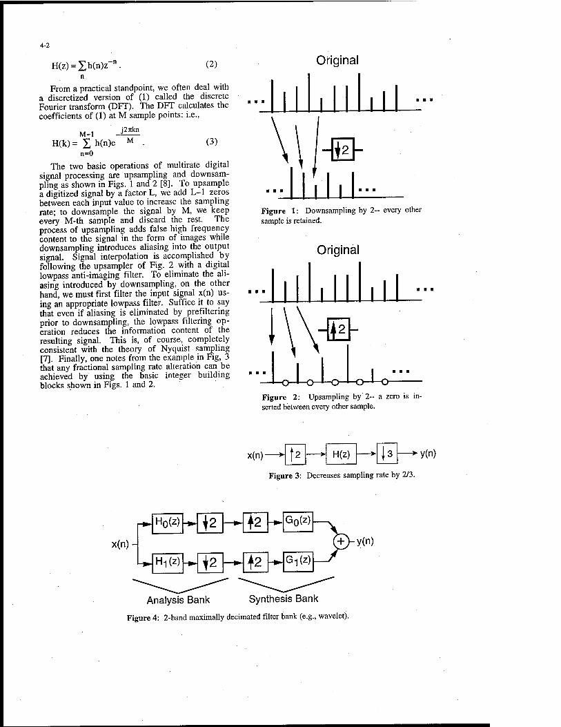
4-2

H(z) = Xh(n)z" (2)

From a practical standpoint, we often deal with a discretized version of (1) called the discrete Fourier transform (DFT). The DFT calculates the coefficients of (1) at M sample points: i.e.,

j27rkn M-l

H(k)= X h(n)e M

n=0 (3)

The two basic operations of multirate digital signal processing are upsampling and downsampling as shown in Figs. 1 and 2 [8]. To upsample a digitized signal by a factor L, we add L-l zeros between each input value to increase the sampling rate; to downsample the signal by M, we keep every M-th sample and discard the rest. The process of upsampling adds false high frequency content to the signal in the form of images while downsampling introduces aliasing into the output signal. Signal interpolation is accomplished by following the upsampler of Fig. 2 with a digital lowpass anti-imaging filter. To eliminate the aliasing introduced by downsampling, on the other hand, we must first filter the input signal x(n) using an appropriate lowpass filter. Suffice it to say that even if aliasing is eliminated by prefiltering prior to downsampling, the lowpass filtering operation reduces the information content of the resulting signal. This is, of course, completely consistent with the theory of Nyquist sampling [7]. Finally, one notes from the example in Fig, 3 that any fractional sampling rate alteration can be achieved by using the basic integer building blocks shown in Figs. 1 and 2.

Original

ü

Figure 1: Downsampling by 2~ every other sample is retained.

Original

Figure 2: Upsampling by 2- a zero is inserted between every other sample.

x(n)- t* H(z) 13 y(n)

Figure 3: Decreases sampling rate by 2/3.

r*. Ho(z) -► \2 -► +2 -*-Go(z) -

x(n)-

LHI(Z)* \2 -M2 -►Gi(z)-

Analysis Bank Synthesis Bank

Figure 4: 2-band maximally decimated filter bank (e.g., wavelet).

4-3

3. Maximally decimated filter banks

3.1 2-band Systems

Using the multirate operators introduced in Section 2, we can now describe the maximally decimated filter bank. A 2-band analysis/synthesis system is shown in Fig. 4 where H„(z) is a lowpass filter and H,(z) is highpass. Note that because of the downsampling operations performed in the analysis filter bank, the sampling density in the transform or subband domain is exactly the same as it was in the original temporal domain. This is especially important for compression applications because each of the transform coefficients must be quantized and coded (i.e., converted into bits) for transmission. This property is also quite useful in other applications as well like pattern classification and signal scrambling [9], [5].

Using basic multirate identities and a little bit of algebraic manipulation on the system of Fig. 3, we find that

H1(z) = z-NH0(-z). (9)

(4) Y(z) = i[H0(z)G0(z) + H1(z)G1(z)] • X(z)

+-[H0(-z)G0(z) + H1(-z)G1(z)]-X(-z)

[8]. The first term in (4) represents the linear time invariant (LTI) response of the combined analysis/synthesis system while the second represents the aliasing introduced into the system by downsampling. This aliasing can be completely canceled, however, if we select

G0(z) = H1(-z), G!(z) = -H0(-z). (5)

Substituting (5) into (4), we see that

Y(z) = T(z)X(z) (6)

where

T(z) = iptto^HjC-z) - H!(z)Ho(-z)] (7)

is the LTI transfer function of the system. In general, T(z) may introduce both amplitude and phase distortion into the reconstructed signal. To achieve perfect reconstruction, T(z) must have the form c-z~n0 for constant c and integer nO.

Perfect reconstruction can be achieved with the appropriate choice of filters H„(z) and H,(z). In particular, assume that H(l(z) is power symmetric. This implies that

■ \ (8) Ho(z)H0(z) + H0(-z)Ho(-z):

where H(z) = H*(z-1], indicating that the filter

coefficients are first time reversed and then con- jugated. To force T(z) to have the desired form

■"" we can thus select

For odd N, (6) reduces to Y(z) = 0.5z NX(z) and perfect reconstruction is achieved! Substituting (9) into (5), the two synthesis filters are now given by

G1(z) = z-NH1(z). (10) G0(z) = z-NH0(z),

Note that all four filters in the system are completely determined by just one of them! The filter bank shown in Fig. 3 was first called the Con- jugate Quadrature Filter Bank when described by Smith and Barn well in [10]. It was not truly popularized, however, until Daubechies showed that such filter banks could be used to build discrete orthogonal wavelet transforms [11].

While the constraint given by (9) must be satisfied if one is to create perfect reconstruction (PR) orthogonal filter banks and wavelets, it does not affect the creation to create non-orthogonal PR systems. In fact, if one wishes to construct a linear phase PR filter bank (or, equivalently, a symmetric wavelet), one must give generally give up orthogonality and equation (9). By doing so one can create instead a biorthogonal system such that

H0(z)Go(z) + Ho(-z)G0(-z) = l. (11)

Two different filters must now be designed such that (11) is satisfied- the remaining two filters are still determined by (5). If we define P(z) = H0(z)G„(z), then (11) becomes

-z) = l (12) P(z) + P(-

which can be satisfied by a half-band or Nyquist filter. Thus, one need only design such a filter and then factor it to create the desired orthogonal or biorthogonal system [8].

{M » G0("z2) 1

T

/

Z"1l r

-1, —i {M 1 G/-Z2) 1

z y r z u {M 1 G (-z2)

2M-1 1

Figure 5: Polyphase implementation of cosine modulated M-band filter bank.

cz

4-4

"0 0.5 1 1.5 2 2.5 3 FREQUENCY

Figure 6: 8-band pseudo QMF bank. Note that only the transition bands of adjacent filters overlap.

1 1.5 2 FREQUENCY

Figure 7: Frequency response of the 8-band analysis/synthesis system whose analysis bank is given by Fig. 6.

4-5

3.2 M-Band Systems

Often it is desirable to split a signal into more than 2 frequency bands. While one can implement an M-band decomposition by successively applying the 2-band filter bank discussed in the last section, it is often more efficient to implement it directly. In fact, the most efficient maximally decimated M-band filter bank capable of achieving good frequency discrimination is the cosine modulated filter bank [8]. Here, one designs a single lowpass prototype filter and then implements the remaining filters by using cosine waveforms to modulate this prototype to higher frequency bands. Figure 5 shows the computationally efficient polyphase implementation of an M- band cosine modulated filter bank (the powers of z"1 denote delay elements or shift registers). Note that the filter coefficients belonging to the lowpass prototype filter H(z) are uniformly distributed amongst the polyphase subfilters Gk(z

2). Thus, the complexity of implementing all M filters is equal to that of the original prototype filter H(z) plus the cost of implementing the Mx2M transform T. The elements of the transform matrix T are given by

tkn = 2 cos(-^ (k + 0.5)(n - ^) + 9k), M 2

(13)

where 6k =(-1) rc/4 and N is the order of H(z). This transform can be implemented very efficiently using a 2M-point FFT plus a few additional operations.

1 1 ■■■! T \

g

1

0 91 92M-1

z-1 z-1 z-1

T T — T T \

=

Audio In-*" BUFFER (2M)

Figure 8: Relationship between LOT and modulated cosine filter bank.

The first filter banks designed along the lines of Fig. 5 were called pseudo-QMF or generalize QMF banks, and they did not achieve perfect reconstruction. Instead, they only cancel aliasing between adjacent frequency subbands, and they introduce a small amount of amplitude distortion into the reconstructed output. Figure 6 shows the analysis filters of an 8-band pseudo QMF bank. Note that only the transition bands of adjacent filters overlap-- the passbands and transition bands of all non-adjacent filters are in the stop- band. Thus, it really is sufficient just to cancel aliasing between adjacent bands. Figure 7 shows the frequency response of the combined analysis/synthesis system. While there is some amplitude distortion, its magnitude is extremely small. Thus, despite its minor flaws, the pseudo-QMF bank has been widely used in a variety of applications, most notably MPEG (motion picture experts group) audio Layers 1, 2, and^. 3 (MP3). More recently, various authors have found ways of designing the prototype filter H(z) so that perfect reconstruction can also be achieved within the framework of Fig. 5 [12].

u ■

H„

Hv

Hh

— low-low band

♦ low-high band

| 2 — high- low band

high-high band

Figure 9: 4-band 2D multirate filter bank- one level of wavelet decomposition.

4-6

It should also be noted that the cosine modulated filter bank of Fig. 5 can be specialized to the lapped orthogonal transform (LOT) or Local Cosine Transform (LCT). To see this, consider Fig. 8. Here, the polyphase subfilters have been replaced by single scalar coefficients. These coefficients are simply the window weights required to implement a LOT having a 50% overlap between adjacent windows. In the figure, the polyphase network acts exactly like a shift register in which half of the samples are replaced with new samples every clocking cycle.

4. Applications

4.1 Wavelet-Based Image Compression

The current standards for image and video compression, JPEG (joint photographies experts group) and MPEG, are both transform coders centered around an 8x8 blocked DCT [1], [2]. More recently, image compression algorithms based on the wavelet transform have gained prominence in both research and development because of their ability to operate effectively over a wide range of compression ratios [13]. [14]. In fact, a single wavelet-based algorithm can be constructed which operates efficiently for both lossless and highly lossy compression [15], [16]. The basic 2-dimensional (2D) wavelet transform used for image compression is constructed by cascading two ID filter banks of the type shown in Fig. 4 so that the first one operates in the vertical direction and the second in the horizontal direction. The 4-band 2D filter bank thus created is shown in Fig. 9 where the subscripts denote the direction of operation of the low (L) and high (H) pass filters. To create a complete wavelet transform, we iterate the filter bank shown in Fig. 9, successively decomposing the low-low band. Figure 10 shows the subband or wavelet coefficient mapping which results from 3 such iterations. To further illustrate this point, Figure 11 shows the wavelet decomposition of an actual image.

The process of wavelet-based compression is illustrated in generic terms by Fig. 12. First the image is transformed and then the transform coefficients are appropriately quantized (eliminating information content) and coded (eliminating redundancy and converting into bits). To reconstruct an approximation of the image, we decode the bit stream and perform an inverse wavelet transform (IDWT) which is simply the synthesis filter bank corresponding to the analysis bank of Fig- 9.

Of particular interest is a class of wavelet-based image compression algorithms called 'embedded' coders [13]-[16]. In an embedded coder, a bit stream is generated and transmitted in order of importance-- i.e., the most important bits are sent first. Figure 13 illustrates this concept. Embed- ded bit streams are useful in a number of ways: 1) if transmission terminates prematurely, we can still reconstruct an image of the best possible quality with the bits we received, 2) unequal error protection coding is easily achieved in a dynamic fashion, and 3) communications channels with fixed bit rates are easily supported. All of these traits are useful in military applications because the communications channels of interest are primarily RF and are likely to be operated in an un- stable and noisy environment.

CD

f LL2 LH2

LH! LH0

HL2 HH£

HL-! HH!

HL0 HH0

Figure 10: Wavelet coefficient or subband mapping.

Figure 11: Wavelet decomposed image.

While a number of embedded coding algorithms have been developed [13]-[15], we describe here the embedded zerotree wavelet (EZW) approach which was the first developed and is still one of the best [13]. The fundamental observation around which this coding algorithm is centered is that there is a strong correlation between insignificant coefficients at the same spatial locations in different wavelet scales— i.e., if a wavelet coefficient at a coarser scale is zero, then it is more likely that the corresponding wavelet coefficients at finer scales will also be zero. Figure 14 shows a 3-level, 2D wavelet decomposition and the links which define a single zerotree structure. If the wavelet coefficient at a given scale is zero along with all of its descendants (as shown in Fig. 14), then a special symbol indicating a zerotree root (ZTR) is transmitted, eliminating the need to transmit the values of the descendants. Thus, the correlation of insignificance across scales results in a net decrease in the number of bits transmitted.

Image 2D Wavelet Transform Quantize Code

4-7

-bits

(a)

bits- Decode IDWT Reconstructed Image

(b)

Figure 12: Wavelet compression and decom- pression.

D «

<Nfl. krrrp

Figure 14: Parent-child relationships amongst zerotree coefficients.

4S|st^'.2it!

i;v IöL;^W Mtf4' * t lEfi^^n -""" "V .>;'?"'"• • [m <<'"J$2b!k.-~' l*wj«BBitt.-îiTt ̂ .IlL^.uüi^^^^

TRANSMITTER

5242 bytes

RECEIVER

Bits Received

Figure 13: Embedded image compression.

4-8

lnput_ Image

Wavelet Analysis

Encoder Create

Dominant Symbols

T=T/2

{Repeat until \ out of bits j

Create Refinement

Symbols

Bits Out

Bits In"

Lossless Decoder

Decoder Decode

Dominant Symbols

T=T/2

{Repeat until stopped

Decode Refinement

Symbols

Wavelet Synthesis

JDutput Image

Figure 15: Encoder and decoder for an embedded image compression algorithm.

In order to generate an embedded code (where information is transmitted in order of importance), Shapiro's EZW algorithm scans the wavelet coefficients in a bit-plane fashion. Starting with a threshold determined from the magnitude of the largest coefficient, the algorithm sweeps through the coefficients, transmitting the sign (+ or -) if a coefficient's magnitude is greater than the threshold (i.e., it is significant), a ZTR if it is less than the threshold but the root of a zerotree at the coarsest possible scale, or a 0 otherwise— this is the dominant pass. Next, for the subordinate pass all coefficients deemed significant in the dominant pass are added to a second subordinate list which is itself scanned, adding one bit of resolution to the decoder's representation of each significant coefficient. Symbols generated by these two passes are then passed through a lossless arithmetic coder to extract further statistical redundancy. After this, the threshold is halved and the two passes are repeated with those coefficients having been found significant previously being replaced by zeros in the dominant pass (so that they do not inhibit the formation of zerotrees in subsequent iterations). The process continues until the bit budget is exhausted; at this point, the encoder transmits a stop symbol and its operation is terminated.

The decoder, on the other hand, simply accepts the bit stream coming from the encoder, progressively building up the significance map and

the subordinate list in the exact same way as they were created by the encoder. Because of this precise synchronization, the resolution enhancement bits transmitted during the subordinate pass do not need any location specifiers— the decoder knows the exact transmission order of these bits because it has reconstructed the same subordinate list as the encoder had at that point in the process. The encoding and decoding processes described here are illustrated by the block diagrams shown in Fig. 15. Figure 16 illustrates the advantages of wavelet-based compression over JPEG at high compression ratios.

4-9

JPEG CR = 51:1 Wavelet

PSNR = 23.8 dB PSNR = 24.5 dB

Figure 16: JPEG versus EZW at a compression ratio of 51:1. Objective comparison metric is peak signal to noise ratio (PSNR).

(a) (b)

Figure 17: (a) Reconstruction of image compressed by 160:1 ratio. Again, squares have been added to highlight enhanced regions, (b) Error residual between reconstructed and original images where white areas in residual denote large errors.

(a) (b)

Figure 18: (a) Compressed with space-frequency weighting by 32:1 ratio; (b) Compressed without weighting. Note that our texture detection algorithm is designed to be selective- it only identified the orchard in the upper left-hand corner of the image but not the one in the lower right-hand corner.

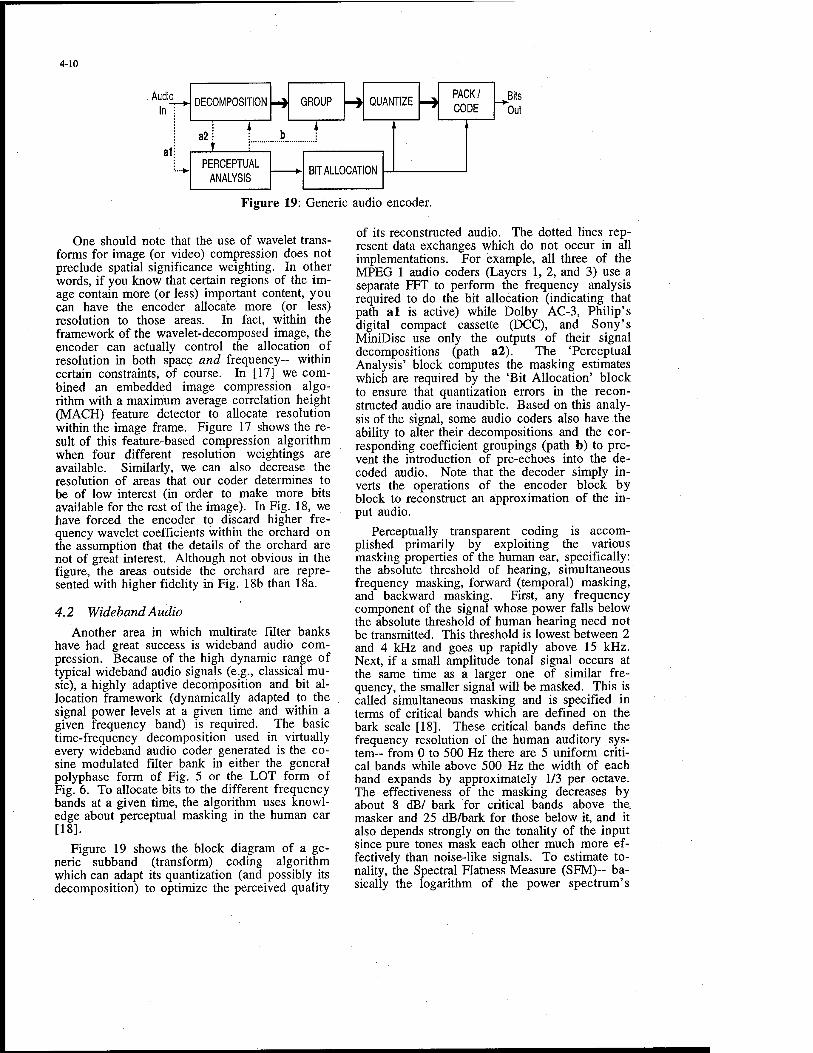
4-10

udio

InT^ DECOMPOSITION -* GROUP QUANTIZE

PACK/ CODE

alj a2; b

i i , ,

t ;

PERCEPTUAL ANALYSIS

RIT Al 1 nPATIHM

^Bits Out

Figure 19: Generic audio encoder.

One should note that the use of wavelet transforms for image (or video) compression does not preclude spatial significance weighting. In other words, if you know that certain regions of the image contain more (or less) important content, you can have the encoder allocate more (or less) resolution to those areas. In fact, within the framework of the wavelet-decomposed image, the encoder can actually control the allocation of resolution in both space and frequency- within certain constraints, of course. In [17] we combined an embedded image compression algorithm with a maximum average correlation height (MACH) feature detector to allocate resolution within the image frame. Figure 17 shows the result of this feature-based compression algorithm when four different resolution weightings are available. Similarly, we can also decrease the resolution of areas that our coder determines to be of low interest (in order to make more bits available for the rest of the image). In Fig. 18, we have forced the encoder to discard higher frequency wavelet coefficients within the orchard on the assumption that the details of the orchard are not of great interest. Although not obvious in the figure, the areas outside the orchard are represented with higher fidelity in Fig. 18b than 18a.

4.2 Wideband Audio

Another area in which multirate filter banks have had great success is wideband audio compression. Because of the high dynamic range of typical wideband audio signals (e.g., classical mu- sic), a highly adaptive decomposition and bit allocation framework (dynamically adapted to the signal power levels at a given time and within a given frequency band) is required. The basic time-frequency decomposition used in virtually every wideband audio coder generated is the cosine modulated filter bank in either the general polyphase form of Fig. 5 or the LOT form of Fig. 6. To allocate bits to the different frequency bands at a given time, the algorithm uses knowledge about perceptual masking in the human ear [18].

Figure 19 shows the block diagram of a generic subband (transform) coding algorithm which can adapt its quantization (and possibly its decomposition) to optimize the perceived quality

of its reconstructed audio. The dotted lines represent data exchanges which do not occur in all implementations. For example, all three of the MPEG 1 audio coders (Layers 1, 2, and 3) use a separate FFT to perform the frequency analysis required to do the bit allocation (indicating that path al is active) while Dolby AC-3, Philip's digital compact cassette (DCC), and Sony's MiniDisc use only the outputs of their signal decompositions (path a2). The 'Perceptual Analysis' block computes the masking estimates which are required by the 'Bit Allocation' block to ensure that quantization errors in the reconstructed audio are inaudible. Based on this analysis of the signal, some audio coders also have.the ability to alter their decompositions and the corresponding coefficient groupings (path b) to prevent the introduction of pre-echoes into the de- coded audio. Note that the decoder simply in- verts the operations of the encoder block by block to reconstruct an approximation of the input audio.

Perceptually transparent coding is accomplished primarily by exploiting the various masking properties of the human ear, specifically: the absolute threshold of hearing, simultaneous frequency masking, forward (temporal) masking, and backward masking. First, any frequency component of the signal whose power falls below the absolute threshold of human hearing need not be transmitted. This threshold is lowest between 2 and 4 kHz and goes up rapidly above 15 kHz. Next, if a small amplitude tonal signal occurs at the same time as a larger one of similar frequency, the smaller signal will be masked. This is called simultaneous masking and is specified in terms of critical bands which are defined on the bark scale [18]. These critical bands define the frequency resolution of the human auditory system- from 0 to 500 Hz there are 5 uniform critical bands while above 500 Hz the width of each band expands by approximately 1/3 per octave. The effectiveness of the masking decreases by about 8 dB/ bark for critical bands above the masker and 25 dB/bark for those below it, and it also depends strongly on the tonality of the input since pure tones mask each other much more effectively than noise-like signals. To estimate tonality, the Spectral Flatness Measure (SFM)~ ba- sically the logarithm of the power spectrum's

4-11

L

c

I" i: i,

■So

fli! TH

|

Spread Spectrum

Signal

K+>-K+)

noise interference

Spread Spectrum Correlator Bit stream

Time- Frequency Transform

Interference Excision

Inverse Transform

Spread Spectrum Correlator Bit stream

Figure 20: Time-frequency based interference excision. Original signal enters noisy communications channel at left. Signal output (to the right) at the top is the bit stream produced if interference is not excised while the one at the bottom has been denoised. Note the clear correlation spike in the bottom signal (indicating a good signal lock) and the lack of such a spike in the upper signal.

4-12

geometric mean divided by its arithmetic mean- is generally employed [19]. Specifically, a ratio of the current SFM to the SFM of a maximally tonal input is used to compute the tonality of the current block of samples, and this tonality coefficient biases the masking threshold upward for highly tonal signals or downward for noise-like signals.

The final perceptual effects which must be considered in the design of the coding algorithm are forward and backward temporal masking. Forward masking occurs when the masking signal ends before the masked signal begins while backward masking is the exact opposite. Per- ceptual studies have shown that forward masking is the more effective of the two by a wide margin [18]. While most of the currently available coding algorithms claim to 'exploit' forward and backward masking, this statement is somewhat misleading. Explicitly, they exploit simultaneous masking to achieve bit rate reductions through adaptive bit allocation while implicitly exploiting forward masking to conceal the effects of time- frequency blocking on the quantized coefficients. In other words, if the masking signal contained within the block of coefficients ends prematurely, the quantization noise will still be concealed. The situation with backward masking, however, is entirely different since this phenomenon is highly localized around the leading edge of the masker. If blocks of coefficients representing a fixed time-frequency subdivision of the signal are jointly coded, then it is possible for pre-echo to be introduced into the reconstructed audio by the occurrence of a large masker in latter parts of a block. Thus, the goal of the coding algorithm is not so much to exploit backward masking as to compensate for its limitations. In fact, the entire motivation for using temporally adaptive transformations in the encoder (path b in Fig. 19) comes from the need for increased time localization of the quantization errors during sharp at- tacks (i.e., sudden increases in the short time power spectrum of the audio input).

4.3 Time-Frequency Interference Excision

The same transforms we applied in the last section to the rather non-military application of wideband audio compression can also be applied to the problem of removing narrow band interference from a wideband signal [20]. To do this, we first transform the signal using the LOT of Fig. 6 and then analyze the frequency subband, looking for any large concentrations of energy. Since our desired signal is wideband, its energy will not be particularly concentrated in any given band. The energy from a narrowband interference, on the other hand, will be concentrated into certain bands, even if its frequency is hopping or chirping (within certain bounds). Once a band containing a potential interference source is detected, we alter its transform coefficients so as to suppress the interference without introducing new types of distortions into the signal. Note that this is more complicated than simply zeroing the of- fending coefficients since these zeros themselves can introduce false information into the output signal. Finally, the transform coefficients— possibly modified- are inverted, and the denoised signal is then sent on for detection or further processing. A block diagram of the complete system is shown in Fig. 20.

Superimposed on the excision system in Fig. 20 is an example illustrating the advantages of excision. The input spread spectrum signal enters from the left and is corrupted by noise and narrowband interference (effects of the communications channel). The upper branch outputting the signal to the right simply correlates the corrupted signal with the original without denoising. Note that the correlation peak is totally obscured by noise. The signal coming out of the lower correlator, on the other hand, has had its interference detected and removed using time-frequency methods [21]. Here, the correlation peak at the output is highly pronounced, indicting that we can easily decode the information bits modulated onto this waveform.

One can also use a windowed Fourier transform in this application. The disadvantage of doing this, however, is summarized by the Balian-

x0(n)

x,(n)

xM-i(n)-

H0 (2) ^M

Hi(z) ^M

HM-I (Z) ^M

- yo(n)

- Yi(n)

-yM-i(n)

Figure 21: COFDM transmission system.

4-13

Low Theorem: it is impossible to design a windowed Fourier transform which simultaneously achieves good time and frequency localization but does not expand the sampling rate of the signal in the transform domain. Thus, to prevent the excision process from introducing artifacts into the reconstructed signal, one must generate and process approximately 50% more transform domain coefficients using a Fourier transform than with the lapped orthogonal cosine transform.

4.4 Code Orthogonal Frequency Division Multiplexing (COFDM)

The basic idea of COFDM is to combine a large number of low bandwidth information sources into a single wide bandwidth signal for transmission [6]. This can be accomplished using the dual structure to the PR filter bank- the perfect transmultiplex. Such a system is shown in Fig. 21 where M narrow bandwidth signals are combined into one signal having M-times more bandwidth. Note that while each of the M input signals is mostly confined to a specific frequency band within the combined signal, there is some overlap because the digital filter are not ideal. Despite this, if the filters Fk(z) and Hk(z) are designed correctly, all cross-talk will be cancelled and no amplitude or phase distortion will be introduced into the output signals: i.e., yk(n) = xk(n) for all k. It is easily shown that if filters Fk(z) are the synthesis filters for an M-band PR filter bank and Hk(z) are the corresponding analysis filters, then the outputs of Fig. 21 will exactly equal its inputs, resulting in a perfect transmultiplexer.

If the impulse responses of the set of filters {fk(n)} are all mutually orthogonal to each other, then the system illustrated by Fig. 21 is truly COFDM. Note that orthogonality of the synthesis filter set {fk(n)} also guarantees orthogonality of the analysis filter set {hk(n)}. If a PR cosine modulated filter bank of the type shown in Fig. 5 is used here, then the filter set {fk(n)} is indeed orthogonal. Higher order filters results in better frequency confinement of the original signal

xk(n) within the composite signal, but they also increase the complexity of the system. To make M as large as possible for a given implementation complexity, the LOT of Fig. 6 is often used. This results in relatively poor frequency localization of a given narrowband input within the broadband composite signal but does not appear to cause any serious problems within the context of this application.

Europe has already selected this modulation scheme for Digital radio broadcasting and will likely select it for digital television as well. Why? A major advantage is that it is much more robust to multipath phenomena and other forms of frequency dependent interference. Specifically, one can adjust the information flow rate going into each of the M input channels so that every channel operates at exactly its maximum capacity. Thus, a channel that is subject to a great deal of interference would have much less data capacity than one which is not. The data rate for each channel can be adjusted by altering the amount of error correction used in it- i.e., the low rate, interference prone channel expends most of its raw capacity on error protection while the high rate, interference free channel uses more of its capacity to transmit actual data bits. In some cases, there might also be a feedback path from the receiver to the transmitter, allowing the system to adapt to the changing RF environment. Note that numerous variations on this concept have been proposed including wavelet modulation and discrete tone modulations. Both of these use the same basic concept as COFDM, but with different modulation kernels [22].

4.5 Time-Frequency Scrambling

It has been shown in [5] how multirate filter banks can be used very effectively to implement voice scrambling systems based on time- frequency permutation. The most general form of such a system is shown in Fig. 22 where P(z) is the permuter (it is a function of z because it has, in general, memory). Since the subband coefficients are only reordered by P(z) and not, in the-

H(z) \u.

H/z^M

4o*H^

P(z)

Encoder Decoder

Figure 22: Time-frequency scrambling.

4-14

ory, quantized, any perfect reconstruction filter bank can be used for the analysis and synthesis operations in Fig. 22 without loss in the quality of the reconstructed signal. If the signal input to the encoder, x(n), has a frequency distribution which is known to the pirate (e.g., mostly lowpass), then the pirate will be able to use this knowledge to more easily break the permuter's scrambling algorithm. This liability can be eliminated at con- siderably higher cost by passing the permuted signal from P(z) through the synthesis bank and transmitting the output. In this case, the decoder must first pass its received signal through an analysis bank, process it with the inverse permuter, P(z)_*, and, finally, reconstruct the un- scrambled signal. If the filter banks used in the process are perfect reconstruction, the unscram- bled signal will still match the original at the end of this process (barring multiplication roundoff and coefficient quantization errors).

Time-frequency scrambling using maximally decimated multirate filter banks has a number of advantageous properties. Obviously, it obscures the signal in both time and frequency, making it very difficult to decode it even if your opponent has a priori knowledge about the statistics of the signal (at least as long as the filters and synchronization intervals are not know exactly). Fur- thermore, since the filter bank is maximally decimated, the scrambler does not increase the bit rate of the signal. On the minus side, the delay introduced by the permuter P(z) for any given sample must be limited to some maximum value for real-time applications. With 2-way voice communications, for example, it becomes impossible to carry on a conversation if the throughput delay or latency grows too large. If little system latency is allowed, the delay constraint on P(z) permits an opponent to limit his key search and thus decode the data more quickly. Time- frequency scrambling systems are most useful for protecting data whose importance is highly time dependent— i.e., data which is immediately useful but has little long term value. For other kinds of sensitive data,, such time-frequency systems probably do not provide adequate protection.

5. Conclusions

We have discussed some of the basic concepts behind digital multirate systems, focusing on the area of maximally decimated filter banks and wavelets. In particular, we have analyzed the 2- band PR filter bank which implements orthogonal and biorthogonal wavelets. We have also considered the important cosine modulated filter bank, a special case of which is the lapped orthogonal transform or local cosine transform. Finally, we have summarized a number of communications- related applications for such filter banks including wavelet-based image compression, wideband audio compression, noise excision, modulation,

and scrambling. Of course, many other applications for such multirate systems also exist including adaptive filtering, pattern recognition, and channel equalization. In short, multirate digital signal processing plays an important role in modern communications systems, and it will likely become even more critical as digital connectivity increases in the future.

Acknowledgement

The author would like to thank Dr. Grant Han- son for contributing material on time-frequency noise excision and the sponsors at the Office of Naval Research who have facilitated this research.

References

[I] G.K. Walleye, "Overview of the JPEG (ISO/CHIT) still image compression -standard," Proc. of the SPIE, Vol. 1244, pp. 220-33, 1990.

[2] DJ. LeGall, "The MPEG video compression algorithm: a review," Proc. of the SPIE, Vol. 1452, pp. 444-57, 1991.

[3] M. Vetterli and J. Kovacevic, Wavelets and Subband Coding, Prentice Hall PTR, Englewood Cliffs, NJ, 1995.

[4] P. Noll, "MPEG digital audio coding," IEEE Signal Processing Magazine, pp. 59-81, Sept. 1997.

[5] R.V. Cox, D.E. Bock, K.B. Bauer, J.D. Johnston, and J.H. Synder, "The analog voice privacy system," AT&T Technical Journal, Vol. 66, No. 1, Jan.-Feb. 1987, pp. 119-131.

[6] W.Y. Zou and Y. Wu, "COFDM: an overview," IEEE Trans, on Broadcasting, Vol. 41, No. 1, pp. 1-8, March 1995.

[7] A.V. Oppenheim and R.W. Schäfer, Dis- crete-Time Signal Processing, Prentice Hall, Englewood Cliffs, NJ, 1989.

[8] P.P. Vaidyanathan, Multirate Systems and Filter Banks, Prentice Hall, Englewood Cliffs, NJ, 1993.

[9] CD. Creusere and G. Hewer, "Wavelet- based nearest neighbor pattern classification using scale sequential matching," Proc. Asilomar Conf. Signals, Systems and Computers, Pacific Grove, CA, Nov. 1994, pp. 1123-1127.

[10] M.J.T. Smith and T.P. Barnwell, "Exact reconstruction techniques for tree-structured subband coders," IEEE Trans, on Acoustics, Speech, and Signal Processing, Vol. ASSP-34, No. 3, June 1986, pp. 434-440.

[II] I. Daubechies, "Orthonormal bases of compactly supported wavelets," Comm. on Pure

4-15

and Applied Math., Vol. XLI, 1988, pp. 909- 996.

[12] H.S. Malvar, "Modulated QMF banks with perfect reconstruction," Electronics Letters, vol. 26, pp. 906-7, June 1990.

[13] J.M. Shapiro, "Embedded zerotree image coding using zerotrees of wavelet coefficients," IEEE Trans, on Signal Processing, Vol. 41, No. 12, Dec. 1993, pp. 3445-3462.

[14] A. Said and W.A. Pearlman, "An image multiresolutional representation for lossless and lossy compression," IEEE Trans, on Image Proc, Vol. 5, No. 9, Sept. 1996, pp. 1303-1310.

[15] A. Zandi, J.D. Allen, E.L. Schwartz, and M. Boliek, "CREW: Compression with reversible embedded wavelets," Proc. Data Compression Conference, 1995, pp. 212-221.

[16] CD. Creusere, "Spatially partitioned lossless image compression in an embedded framework," Conf. Rec. 31st Asilomar Conf. on Signals, Systems, and Computers, Pacific Grove, CA, Nov. 1997, pp. 1455-59.

[17] CD. Creusere and A. Van Nevel, "Auto- matic target recognition directed image compression," to appear in the Journal of Aircraft.

[18] E. Zwicker and H. Fasti, Psychoacoustics. Berlin: Springer-Verlag, 1990, pp. 141-147.

[19] J.D. Johnston, "Transform coding of audio signals using perceptual noise criteria," IEEE J. Select. Areas Commun., vol. 6, pp. 314-23, Feb. 1988.

[20] J.H. Young and J.S. Lehnert, "Performance metrics for windows used in real-time DFT-based multiple-tone frequency excision," IEEE Trans, on Signal Processing, vol. 47, No. 3, pp. 800-12, March 1999.

[21] G. Hanson, "Adaptive time-frequency jammer excision using local cosine transforms," Proc. 1999 National Technical Meeting & 19th Biennial Guidance Test Symposium (classified volume), Jan. 1999, San Diego, CA.

[22] A.N. Akansu and X. Lin, "A comparative evaluation of DMT (OFDM) and DWMT (DSBMT) based DSL communications systems for single and multitone interference," Proc. Int. Conf. on Acoustics, Speech, and Signal Proc, Vol. 6, pp. 3269-72, 1998.

5-1

Multisensor Signal Processing in the Framework of the Theory of Evidence

Alain Appriou

ONERA BP 72, 92322 Chätillon Cedex, France

Tel.: +33 1 46 73 49 19 ; Fax : +33 1 46 73 41 67 E-mail: [email protected]

Summary: In most of the requirements met in situation assessment, multisensor analysis has to be able to recognize in adverse conditions one situation out of a set of possibilities concerning for instance either localization, identity, or matching hypotheses. To do so, it uses measurements of more or less doubtful origin and prior knowledge that is understood to be often poorly defined, and whose validity is moreover difficult to evaluate under real observation conditions. The present synthesis proposes a generic modeling of this type of information in the framework of the theory of evidence, with closer attention being paid to the different natures of data processed in common cases. This modeling in then used to elaborate processing methods able to face specific problems that may arise when multisensor systems are implemented to achieve functions like detection, classification, matching of ambiguous observations, or tracking. Crucial practical problems are more specifically dealt with, such as appropriate combination processing and decision making, management of heterogeneous frames of discernment, and integration of contextual knowledge. Furthermore, the interest of a global functional approach at low level, possible in that framework, is emphasized.

1 Data Uncertainty in Multisensor Systems

Sensors are mainly associated in order to get benefit of their complementarity. Different kinds of advantages may be expected:

- ability to face a more important set of situations, as one sensor may be efficient while an other one is not because of particular counter-measures, physical phenomena, conditions of observation, or lack of suitable knowledge (learning,...);

- saving of time thanks to task sharing and cooperation between specific functions;

- discrimination capacity improvement as a result of observation conjunction when only partial information is locally available (classification, localization,...).

Consequently, when analyzing a situation, the available sensors are most often used under conditions that induce uncertainties at different levels :

- measurements may be imprecise, incomplete, or ill-suited to the problem,

erroneous,

- observations may be ambiguous, either in space or in time (e.g. position, velocity, or feature measurements provided by two different sensors are not necessarily related to a same object),

- prior knowledge (generated by learning, models, descriptions, and so forth) may be incomplete, poorly defined, and especially more or less representative of reality, in particular in light of the varying context.

Moreover, the disparity of the data delivered by the various sensors, which is intended to remedy the individual insufficiencies of each, requires a detailed evaluation of each of them, based on any exogenous information that might characterize their pertinence to the problem at hand and the context investigated, while such information is itself often very subjective and imprecise.

Theories of uncertainty offer an attractive federative framework in this context. But they run up against a certain number of difficulties in practice : interpretation and modeling of the available information in appropriate theoretical frameworks, choice of an association architecture and combination rules, decision principles to be adopted, constraints concerning the speed and volume of the necessary computations.

To provide solutions to these questions, we will first consider a generic problem in which we attempt to characterize the likelihood of / hypotheses Hi theoretically listed in an exhaustive and exclusive set E. These hypotheses may typically concern the presence of entities, target or navigation landmark identities, vector or target localization, or the status of a system or of a situation.

Such a likelihood function may then be integrated either into :

- a choice strategy, to declare the most likely hypothesis (target identification, intelligence, and so on),

- a filtering process (such as target tracking or navigation updating),

- a decision aid process for implementing means of analysis, electronic warfare, or intervention.



5-2

The likelihood functions we want have to be developed from the data provided by J sensors Sj. Each of them is assumed to be associated with processes that extract a measurement or a set of measurements sj, pertinent to the targeted discrimination function, from the raw signals or images it generates.

The developments presented are conducted in the theory of evidence framework [1], which provides the broadest and best-suited tools for the interpretation and the processing of the data considered. It is also the most federative in terms of synergy between the different theoretical frameworks that may be involved together. Appendix A gives a few basic notions that will be used in the following.

We first propose a common solution to the generic modeling problem introduced formerly, that is afterwards particularized when closer attention is paid to the different natures of data processed in common cases. This modeling in then used to elaborate suitable classification methods, thanks to appropriate combination processing and decision making. Furthermore, specific problems met in multisensor systems are considered, such as management of heterogeneous frames of discernment, integration of contextual knowledge, and matching of ambiguous observations. Finally, the interest of a global functional approach at low level, possible in that framework, is emphasized with the implementation a tracking process that manages directly discrimination features.

2 Modeling of Input Data

2.1 Generic Model

In the framework of the generic problem we will be considering first, we assume that each measurement SJ

can be used to generate / criteria Cy, on the basis of any a priori knowledge, having values in [0,1] capable of characterizing the likelihood of each hypothesis Hj. A quality factory with values in [0,1] is also associated with each likelihood Cy. Its purpose is to express the aptitude of the criterion Cy to discriminate the hypothesis H\ under the given observation conditions, on the basis of a dedicated learning process or exogenous knowledge. This factor includes mainly the confidence that can be accorded to the validity of the a priori knowledge used for generating Cy. As concerns, for example, the representativity of a learning process in a varying context, it will typically depend on the quality, volume, and suitability of the available preliminary data as regards the situation effectively met.

Furthermore, we consider here the practical case of interest when the criteria Cy are generated by separate information channels, in agreement with the fact that they are characterized by different levels of reliability qy. We also assume that we are in the most frequently

encountered context where the criteria Cy taken separately are always at least of refutation value, in the sense that, when zero, this guarantees that the associated hypothesis Hi is not verified.

This leads to a formal construction of the problem on the basis of two axioms [2], [3]:

Axiom 1 : Each of the PJ pairs [Cy,qy] constitutes a distinct source of information having the focal elements Hi, ~^Hi, and E, in which the frame of discernment E represents the set of the / hypotheses Hi

Axiom 2 : When Cy = 0, Cy being valid (qy = 1), we can assert that H\ is not verified.

Axiom 1 requires that I*J mass functions my(.) be generated from the I*J respective pairs [Cy,qy]. For each, the mass of focal elements Hi, ^Hj, and E is at first defined by the value of the corresponding criterion Cy, which can be interpreted only in terms of credibility or plausibility of///. Axiom 2 then limits the number of allowable interpretations to two. The first interpretation leads to:

Cry(Hi) = 0 and Ply(Hi) = Cy

and the second to :

Crij(Hi) = Ply(Hi) = Cy

(2.1)

(2.2)

Then, including the confidence factor qy for Cy by discounting at the rate (l-qy) provides the desired mass function my(.). This leads to the two possible models :

Model 1 :

my(Hi) = Q my(-Hi) = qy*(l-Ciß mij(E)=l-qy*(l-Cij)

Model 2:

my(Hi) = qy*Cy my(-Hi) = qy*(l-Ciß my{E) = l-qy

(2.3) (2.4) (2.5)

(2.6) (2.7). (2-8)

A mass function m(.) synthesizing all the evaluations is then obtained by computing the orthogonal sum of the different mass functions my(.) in the framework of each model:

m(.) = fcB my(.) (2.9)

It should be noted that Model 1 is consonant. Furthermore it satisfies the minimum of specificity measure [4].

5-3

The practical determination of the Cy and qy terms is of course a problem specific to the type of application at hand. The following in this section 2 provides expressions of Cy for the different natures of data processed in common situations. The determination of qij is discussed in sections 3 and 5.

2.2 Model With Statistical Learning

We have to consider different kinds of relation between the sensor observations and the discrimination features that are characterized by previous learning.

2.2.1 Precise and Reliable Observation

The problem dealt with here assumes that each of the measurements sj is directly one of the discrimination features exploited or a deterministic function of it, so that for each of them a learning of their a priori probability distribution p(sj/Hj), under the various hypotheses Hj, is available. Most systems do in fact allow a certain number of preliminary measurements in different real or simulated situations, from which histograms can be generated to get a numerical or analytical model of the distributions p(sj/Hj). The I*J values of probability density p(sj/Hj) associated respectively with the J local measurements sj constitute the inputs for the processes discussed hereafter.

If we consider the most common case, where the measurements SJ can be assumed to be statistically independent, since the sensors are generally chosen for the complementary nature of the data they generate, the likelihood of each hypothesis Hj can be established immediately by the Bayesian approach, which typically calls for an evaluation of the a posteriori probability P(Hj/s l,...,sj) of each hypothesis Hf using :

P(Hils\,...,sj) = {[Up(sj/Hi)]*P(Hi)} 11 {[Up(sj/Hk)]*P(Hk)} (2.10)

J k J

in which P(Hj) designates its a priori probability.

However, this kind of approach quickly runs into difficulty when the real observation conditions differ from the available learning conditions, or when the measurement bank is not sufficient for a suitable learning process. The lack of control that can be seen at this level in most applications leads to distribution models that turn out to be more or less representative of the data actually encountered. In addition, it is often difficult to find a set of a priori probabilities P(Hj) capable of reflecting the real situation with fidelity.

So we want to find a modeling based solely on the knowledge of pißjlHi) and capable of integrating any information concerning the reliability of the various

distributions, whether this comes from a more or less partial knowledge of the observations conditions or from a qualification of a data bank.

According to the generic approach introduced in section 2.1, any available qualitative information is assumed to be synthesized in the form of I*J coefficients qye[0,l], each being representative of a degree of confidence in the knowledge of each of the I*J distributions p(sj/Hj).

Dealing with this problem in the terms of evidence theory requires finding, for each source Sj, a model of its I a priori probabilities p(sj/Hi) and their / respective confidence factors qy in the form of a mass function mj{), characterized by a credibility function Crj(.), and by a plausibility function PljQ. Since the sources Sj are distinct, a global evaluation m(.) can then be obtained by computation of the orthogonal sum of the «/(.). The appropriate frame of discernment is of course the set of the I a priori listed hypotheses Hj.

To do this, we propose to conduct an exhaustive and exact search of all the models that might satisfy three fundamental axioms [2], [5]. These three axioms are chosen beforehand on the basis of their legitimacy in most of the applications concerned. They are :

Axiom 3 : Consistency with the Bayesian approach in the case where the learned distributions p(sj/Hj) are perfectly representative of the densities actually encountered (qij=l, Vy) and where the a priori probabilities P(Hj) are known.

Axiom 4: Separability of the evaluation of the hypotheses 77/; that is, each probability must be considered as a distinct source of information generating a particular mass function my{), mainly capable of integrating the confidence factor qy specific to it. We thus require that each mass function mj(.) be the orthogonal sum of the I mass functions my(.) considered for ze[l,/]. Also, considering the way the p(sj/Hj) probabilities are generated, the focal elements of the mass function myQ can be only Hi, ->Hj,- or E, where the frame of discernment E is the set of hypotheses Hj.

Axiom 5 : Consistency with the probabilistic association of the sources; for independent sources Sj and densities pisjIHi) perfectly representative of reality, the modeling procedures retained must lead to the same result if we compute the orthogonal sum of the m/(.) modeled from the p(sjlHi) or if we model directly the joint probabilities p(s \,... ,sjHj) given by :

P{S\,...,sjlHi) = Y[p{sjlHi)

j

(2.11)

The search for models satisfying these three axioms is presented in appendix B by progressively restricting the

5-4

set of possible models, taking the axioms into account in the order stated.

It appears that only two models satisfy the three desired axioms. Both meet the decomposition :

mj(.)= © mjj(.)

Model 1 is particularized by :

»,}■(#/) = 0

mi/rHj) = qy* {1-Rfp(sj/Hj)} my{E) = l-qij+gij*Rj*p(sj/Hi)

and Model 2 by :

(2.12)

(2.13) (2.14) (2.15)

mi/Pi) = qij*Rj*p{sjlHi)l{\+Rj*p{sjlHi)} (2.16) mijfrHi) = qylil+RfpisjIHi)} (2.17) my(E)=l-qy (2.18)

In both cases, the normalization factor Rj is simply

constrained by:

Rj e [0, (max{p(s/tf;)})-l]

sj,i

(2.19)

Nevertheless, the specificity of the function used to generate model 2 allows Rj to be simply a positive number for this model in practice.

We may verify that this result is in feet a special case of the generic solution discussed in section 2.1. Both models provided by (2.3) to (2.5) and (2.6) to (2.8) in section 2.1 are strictly equivalent to the two models found here in (2.13) to (2.15) and in (2.16) to (2.18), if we adopt the following respective definitions for the Cy :

for model 1 : Cy = Rj*p(sj/Hj) (2.20)

for model 2 : Cy = Rfp(sjlHi)l[\+Rj*p(sjlHj)] (2.21)

in which Rj is still, of course, the normalization gain constrained by (2.19).

This outcome is in fact legitimate if we note that Axiom 1 is expressed directly by Axiom 4, and that the solutions required by Axioms 3 and 5 automatically verify Axiom 2. Axioms 3 and 5 simply make it possible to specify the inclusion of the particular information p{sjlH{) in the expression of the criterion Cy.

Lastly, when the data SJ are discrete values (local identity declarations, for example), the generalized Bayes theorem defined by P. SMETS in the framework of evidence theory [6] can be applied, for the case of statistical learning, to the cartesian product between the set of data and the set of hypotheses. It then strictly yields Model 1 developed here. Correlatively, we have

to note that the model 1, once again, minimizes the specificity measure criterion [4].

2.2.2 Uncertain Observation

We assume now that the measurements SJ are uncertain observations of discrimination features uj, so that only their a priori probability distribution p(sjluj) is known. This may simply be the classical characterization of a measurement error. Furthermore, for each of the discrimination features uj themselves, a learning of their a priori probability distribution p(ujlH{) under the various hypotheses Hj is as formerly available.

If we note that:

pisjIHi) = jp(sj/uj)*p(uj/Hj) duj (2.22)

then the results of section 2.2.1 can be directly extended so that the generic solution provided in section 2.1 holds with :

for model 1 : Cy = Rj* Jp(sj/uj)*p(uj/Hj) duj (2.23)

for model 2 : Cy = Rj*[ jp(sj/uj)*p(uj/Hj) dw/]/ [\+Rj* jp{sjluj)*p{ujlHi) duj] (2.24)

where the normalization factor Rj is now constrained by :

Rj e [0,(max{jp(sj/uj)*p(uj/Hi)duj})-l] (2.25) Sj,i

2.2.3 Imprecise Observation

In this case the measurements SJ are imprecise observations of the discrimination features UJ, so that they only provide a fuzzy membership function /Jj(uj). For each of the discrimination features UJ, a learning of their a priori probability distribution p(uj/H{) under the various hypotheses Hj remains available, as formerly.

We can here express :

p(sj/Hj) = J /Jj(uj)*p(uj/Hj) duj (2.26)

Once more the results of section 2.2.1 can be directly extended, and the generic solution provided in section 2.1 holds with:

for model 1 : Cy = Rj* \ fij(uj)*p(uj/Hi) dw/(2.27)

for model 2 : Cy = Rj*[ J jij{uj)*p{ujlHi) dw/]/ [l+Rj* J ßj(uj)*p{ujlHi) duj] (2.28)

The normalization factor Rj is now constrained by :

5-5

Rj e [0, (max{ Jßj(uß*p(uj/Hi) dw/})-l] (2.29) s,;i

2.3 Model With Approximate Prior Knowledge

Once again we have to consider the different kinds of relation between the sensor observations and the discrimination features, whereas the latter are now characterized by approximate prior knowledge.

2.3.1 Precise and Reliable Observation

In this case each of the measurements SJ is directly one of the discrimination features exploited, or a deterministic function of it. Nevertheless, the characterization of the different hypotheses Hi in the feature space is now provided by prior knowledge in the form of fuzzy membership functions m(sß. This means that an hypothesis Hf represents for instance an object about which we only know that it is large, slow, or heavy, as regards respectively the size, speed, or weight space.

To elaborate a suitable model, we have first to consider, for each hypothesis ///, ce-cuts Aak of fi&sj) at different decreasing levels 0%. As each a-cut defines a set that includes the previous one, it leads to the following consonant mass function on the measurement space :

m(Aak/Hi) = ccic-ak+l (2.30)

The Generalized Bayes Theorem defined by P. SMETS in the framework of the evidence theory [6] may then be implemented to obtain a mass function on E for each of the measurements s V-

m{Hilsj) = 0 m(rHilsp=\-lli{sj) m(filsj) = lii(sj)

(2.31) (2.32) (2.33)

This mass function is then discounted at the rate (1-qjj), if qij represents our degree of confidence in the prior knowledge fij(sj), to provide the model we are looking for:

mij{Hi) = 0 mij(rHi) = qif[\-m(sß] mifE) = \-qij+qij*ßi(sj)

(2.34) (2.35) (236)

Obviously this result can be expressed by the model 1 obtained for the generic problem in section 2.1, as soon as Cjj is defined by :

Qj = Pi(sj) (2.37)

2.3.2 Uncertain Observation

We assume here that the measurements SJ are uncertain observations of discrimination features UJ, so that only their a priori probability distribution p(sj/uj) is known. Furthermore, for each of the discrimination features uj themselves, a prior knowledge provides the fuzzy membership function ufaiß that characterizes the different hypotheses Hj, as formerly.

On this basis, the possibility theory gives the possibility of each hypothesis H{ for each feature UJ :

n(Hj/uß = p{uß (2.38)

as well as the possibility density of each feature UJ for each measurement SJ :

n(uj/sß = Rfp(sj/uß (2.39)

where Rj is a normalization factor such that:

Rj = [msx.{p(ßj/uß}]-l (2.40)

As a possibility function is simply a consonant plausibility function, on the one hand (2.38) can in fact be deduced from (2.31), (2.32), and (2.33), reminding that in the latter sj is directly the feature UJ, and on the other hand (2.39) can result from (2.12), (2.13), (2.14), and (2.15), when information is considered reliable (qif=\), if the set E of hypotheses becomes the infinite set of the possible values taken by UJ (note that such an evaluation in a continuous framework is only possible for the plausibility function, and thanks to the special nature of the focal elements ofmyQ as defined by (2.13), (2.14), and (2.15)). The normalization factor Rj has simply to be particularized by (2.40), in agreement with (2.19), in order to satisfy the definition of a possibility distribution.

Then, (2.38) and (2.39) allow to elaborate the possibility of each hypothesis Hj for each measurement sj thanks to :

nWsß = suV{IKHi,uj/sj)} (2.41) Uj

which can be developed as :

Tiimisj)=sup{n(Hi/uj)An(uj/sj)} (2.42)

where A stands for the conjunction operator, and finally :

IKHjIsß = sup{mm{fij(uj),Rj*p(sj/uj)}} (2.43) Uj

5-6

As a possibility function is but a particular plausibility function, the corresponding mass function which minimizes the specificity measure [4] can be expressed, after discounting according to the confidence factor qy:

mjj(Hj) = 0 (2.44) mijirHj) = q{j*[l- sup{min{ßi(uj),Rj*p(sj/uß}}]

uj (2.45) mij(E) = l-qij+qij*sup{min{ßi(uj),Rj*p(sj/uj)}}

UJ (2.46)

Once more, this result is obviously the model 1 provided for the generic problem in section 2.1, as soon as Cjj is now defined by :

Cy = sup{mm{Hi(uj),Rj*p(sj/uß}} (2.47)

in which Rj is still given by (2.40).

2.3.3 Imprecise Observation

The measurements SJ are now imprecise observations of

the discrimination features UJ, so that they only provide a fuzzy membership function ßj(uj). Nevertheless, fa- each of the discrimination features UJ themselves, the prior knowledge still provides the fuzzy membership function fifoij) that characterizes the different hypotheses Hi, as formerly.

Wljlsfi = fl/llj) (2.48)

The developments in these conditions are quite similar to those shown in section 2.3.2. The only difference concerns the expression of the possibility density of each feature UJ for each measurement SJ that becomes :

Consequently, this leads once again to the model 1 provided for the generic problem in section 2.1, where Cjj has now to be defined by :

Cij = sup{mm{fij(uj),tij(uj)}} (2.49) UJ

2.4 Summary of the Models Obtained

A complete set of models has been developed in the previous sections, in the framework of the theory of evidence, according to the different kinds of data that have to be combined as regards measurements on the one hand, and prior knowledge on the other hand. All these models are particular cases of the two models provided for the generic problem in section 2.1, thanks to suitable expressions of Cji. The definitions of Cy for the different possible situations are summarized in table 1 for model 1 and in table 2 for model 2.

We may note that tables 1 and 2 furthermore provide expressions of Cjj for a precise and reliable prior

knowledge, i.e. for a prior characterization of hypothesis Hj formalized by a deterministic value uu of the feature UJ. In fact these expressions are simply provided either by statistical learning when p(uj/Hi)=S(uj-uij), or by approximate prior knowledge when /ii(ujj)=l and fii(uj/uf£ujj)=0. Nevertheless we can verify the good coherence at this level between the two approaches in the common case of model 1.

Prior knowledge -» Measurements I

Uij piujIHi) Hi(up

SJ 1 if sj=uij 0 if sjtuij

Rj*p(sj/Hi) Rj constrained by (2.19)

Pfaj)

p(Sj/Uj) Rj*p{sjluij) Rj constrained by (2.19)

Rj* J p(sj/uj)*p(uj/Hi) duj Rj constrained by (2.25)

sup{min{iu/<M/), Rj*p(sj/uj)}} Uj

Rj defined by (2.40)

A#»y) Ufaifi Rj* J flj(uj)*p(uj/Hi) duj Rj constrained by (2.29)

sup {min {ßi(uj), Hj(uj)}} Uj

Table 1. Expression of Cy in generic model 1 for the different kinds of prior knowledge and measurement

5-7

Prior knowledge -> Measurements I

«ij p{ujlHi) ßfaj)

SJ 0.5 if sj=uij 0 if'sjtuij

Rj*p(sj/Hiy[l+Rj*p(sj/Hi)] Rj>0

(*)

p(Sj/Uj) Rj*p(sj/uij)/[l+Rfp(sj/uij)] Rj*[\p(sj/ujrP(uj/Hj)duj]/ [\+Rf lp(sj/uj)*p(uj/Hj) duß

Ri>0

(*)

Ufa/) fJj(.Uij)/[l+IIj(Uij)] Rj*[^j(uß*p(uj/Hi)duß/ [\+Rf JHj(uß*p(uj/Hi) duß Rj>0

(*)

(*) Not consistent

Table 2. Expression of Cy in generic model 2 for the different kinds of prior knowledge and measurement

3 Target Classification

The target classification function consists in recognizing the type of a target, or even identifying it, on the basis of the different discriminating features SJ delivered by the sensors Sj that observe it. So the question is to designate the most likely hypothesis Hi* in E={H\,...,Hi) having regard to this information. Such a decision, which is immediate when a probability can be associated a posteriori with each hypothesis, becomes quite delicate when the evaluations are presented in terms of mass functions of the evidence theory. The whole difficulty revolves around the non- exclusivity of the evaluations, which raises the practical problem of interpretation and relative inclusion of the masses attached to those focal elements of cardinal 2 or greater, in the designation of a unique singleton. This problem, which is general to the evidence theory and unavoidable in the present context, has, as of today, been addressed only by more or less satisfactory intuitive solutions.

So below, we propose three different approaches to the problem of choosing the most likely hypothesis Hf, considering an arbitrary mass function m(.) on the fiame of discernment E={H\,..., Hj}, when no other a priori basis for discriminating among the Hj is retained.

A synthesis of the resulting procedures provides a decision law suited to the classification problem. When applied to the modeled mass functions, this law supplies classification methods of noteworthy interest.

3.1 Minimum of Inconsistency

This approach consists in defining / certain mass functions'«/(.), each of them being respectively focused on each of the / hypotheses Hi of the frame of discernment E (/n/(///)=l). The inconsistency Kj, provided by the orthogonal sum of the mass function mi(.) and the available mass function m(.), reflects their disagreement, and so represents the conflict between the assessment m(.) and the fact that hypothesis Hj is

actually true. According to this, we have to choose the hypothesis Hf that ensures a minimal inconsistency K{. As Kj can be written :

Ki=\-Pl{Hi) (3.1)

in which Pl{) is the plausibility function associated with m(.\ we have to choose the hypothesis that provides a maximal plausibility.

The interest in this inconsistency criterion is confirmed by the idea of entropy that is connected with it [4].

3.2 « Bayesian » Approach

The idea here is to consider a given set of « equiprobable » Bayesian masses mQ(.) on the frame of discernment E (mo(Hj)=l/I, V/'e[l,i]). Endowing this mass function mQ(.) with a role similar to that of equiprobable a priori probabilities in the Bayesian inference, a mass function mc(.) can be determined by orthogonal sum of the mass function mQ(.) and the available mass function TK(.). mc(.) is then a Bayesian mass function defined by :

mc(Hi) = PKHiy{l Pl(Hk)}, ie[l,I\ (3.2) *e[l,/]

mc(.A) = 0, VA*H{ , ie[\J\ (3.3)

in which Pl(.) is the plausibility function associated with m(.). By reference to the maximum a posteriori probability, the decision procedure obviously consists in retaining the hypothesis Hj* that has the maximum mass, and thus the maximum plausibility here again.

Conceptually, the principle of this approach consists in substituting an equal confidence between the singletons of the frame of discernment in place of the total a priori uncertainty, so as to force the discrimination among these elements alone.

5-8

3.3 General Approach of the Decision Problem

Here we look for a solution with reference to a more general decisional context summarized, for example, in [7]. The purpose is to choose one of a number of possible actions to take, ah, on the basis of the evaluation provided by the mass set m(.) on the frame of discernment E.

This choice can be made by maximizing a cost function C(ah) on the set of possible actions, knowing the weight G(an/Bk) assigned to each potential action ah when the

event Bk, a subset of E, occurs :

C(ah)=l {G(ah/Bk)*m(Bk)}

Bk(ZE

(3-4)

The whole difficulty of using such a procedure in practice, and hence its credibility, resides in the evaluation of the weights G(anIBk), which is usually very subjective. While we may in general consider that the weights relative to the singletons Hj of £ are given by the system or user, those relative to the subsets Bk of cardinal 2 or higher must, on the other hand, be determined intuitively, possibly in accordance with a preferred « attitude » [7].

Yet in our case, this subjective character can be greatly attenuated by the one-to-one correspondence we have to establish between the set of actions and the frame of discernment E, as each action ah consists in declaring an hypothesis Hj to be true. So, if there are no specific requirements, the weights are legitimately given by :

G(a//5yt)=l G(aj/Bk) = 0

if if

HieBjc Hj£Bk

(3.5) (3.6)

so as to conform with the associated idea of mass m(Bk) as introduced by the evidence theory, i.e. as an evaluation of one of the elements of Bk, cannot specify of which element of Bk it is.

i.e. though we

Under these conditions, (3.4) also leads to the designation of hypothesis Hf of maximum plausibility as the most likely.

Furthermore, it can be pointed out that this approach is coherent with the most consensual evaluation of the expected loss, among those proposed for instance in [8].

It should also be noted that this decision law is the one that satisfies the constraint emphasized at the end of the developments concerning axiom 3 in appendix B.

For all the models discussed in section 2, as the hypotheses Hi are singletons of the frame of discernment E, the plausibility Pl(Hj) is proportional to the product of the Plkj(Hi) associated with the mkj{.), according to j and k. After normalization by the product of the Plkj(-^Hk) according to j and k, we come to designate Hf by the criterion :

Hf = argimaxiUilmijiHd+miji^Vlmiji-Hd+mijiE)])}] i j (3-8)

This criterion can directly be applied to the two models provided for the generic problem, leading to the two respective solutions :

Solution 1 :

/7/* = arg[max{n[l-^*(l-Cy)]}] (3.9) ' ;'

Solution 2 :

Hf = aTg[max{U([l-qij*(l-C0[l-qifCiß)}] (3.10)

' j

It should be noted that solution 1 also meets a maximum credibility criterion.

The simplicity of the calculations and ease of use of these solutions is worth noting.

Furthermore, if we want to integrate a relative a priori confidence Aye [0,1] respectively in the declaration of each of the different hypotheses ///, or accordingly an expected risk (1-A;) attached to it, we may formalize this knowledge as a supplementary source of information. The plausibility function PloQ of such a subjective source has simply to be defined on E for the singletons Hi, the only information we need in the following, thanks to direct interpretation of the A/:

Pl0(Hi) = Xi (3-11)

Therefore, the criterion of maximum plausibility (3.7) becomes, once the orthogonal sum between />/(.) and PIQQ is computed for the singletons Hi:

3.4 Synthesis

The three approaches presented all converge to the same decisional procedure, which consists in choosing the most likely hypothesis Hj* according to :

tf/* = arg[max {A/*/>/(#/)}]

ie[lj]

and consequently (3.9) and (3.10) become :

(3.12)

Hf = arg[max {Pl(Hj)}] ie[l,r\

(3.7)

5-9

Solution 1 :

Hf = arg[max{A,*n[l-?i7*(l-C,y)]}] (3.13) i j

Solution 2 :

Hi* = aig[max{^*n([ Wi7*(l-C,y)]/[W,/Cy])}] i j (3.14)

Of course, in (3.9), (3.10), (3.13), and (3.14), C,y stands for any of the suitable expressions developed in section 2, according to the nature of the available data.

3.5 Illustration

Figure 1 shows the mean probability of good recognition provided by the simulation of 2 sensors for a problem of discrimination between 2 hypotheses H\ and H2. 1° this very simple example both sensors are similar, as regards either their a priori good discrimination capability, or the unreliability of their learning concerning hypothesis H2, in relation with an anticipated possible evolution of

the context.

Recognition rate 1

0,8 "

0,7 •-

0,5

0,4

Figure 1. Classification with unreliable learning

More precisely, we are in the situation developed in section 2.2.1, and available learnings are given by normal distributions :

P(s\/Hi) = P(s2/Hi) = N(0,\)

P{s\IH2) = P{silH2) = N{6,\) with $11 = ?12 = 1 with 921 =922 = <7

while measurements actually simulated fellow :

P(s\/Hi) = P(s2lHi)=N(0,\) P(si/H2) = N(S,l) , P(s2/H2) = N(2,l)

So in this test sensor 2 has effectively a wrong knowledge about H2, and the reliability of sensor 1 varies in function of the signal 5 due to H2. This is in accordance with the choice of factors q\j that expresses a situation where a severe error concerning H2 may occur simultaneously on both sensors. In this context our attention has to focus on the values of S much lower than 6, i.e. typically S<4. Then the curves of figure 1 emphasize the robustness of our approach (9=0,9), as regards either the probabilistic approach, that is a

particular case of our method 07=1), or each sensor alone, which the probabilistic approach does not achieve.

Moreover, the aptitude of the qjj factors to integrate linguistic or subjective information, considering the low sensitivity of the results to the choice of a given value for these coefficients, must be pointed out [5].

4 Management of Heterogeneous Frames of Discernment

Most often we have to use a sensor Si that provides a mass function m\(.) on a frame of discernment E\, but in fact we need an assessment on a frame of discernment E such that E\ C£, either for immediate decision making, or for combination with other mass functions available on complementary frames of discernment. For instance this may occur in case of incomplete learning, or when some hypotheses are not observable, as regards sensor Si. So we have to express m\(.) on E.

5-10

The basic solution to that problem consists in deconditioning m\(.) from E\ to E (see appendix A). The advantage of this solution is that it does not require any particular condition, and therefore can be always implemented. Nevertheless, as we shall see, in most cases it is not the best approach.

A first alternative solution is possible when m\{.) is obtained from modeling developed in section 2, i.e. it is the orthogonal sum, according to /, of the mass functions JB/I(.) defined by (2.3), (2.4), and (2.5), or by (2.6), (2.7) and (2.8). Then, the absence of any C/i, characterized by qn=0, does amount to ignoring the corresponding mass function w/l(.), as it becomes a trivial mass function (m;i(E)=l), and is therefore a neutral element of the orthogonal sum. Moreover, the other elementary models /w;i(.) are not modified whatever the frame of discernment is, as their focal elements integrate in -'Hi any hypothesis that is different from Hf, so that -•Hf may naturally include all the missing hypotheses. Compared with the previous method of deconditioning at the level of m\(.), this approach ensures less losses of specificity measure [4] as regards initial information.

If m\(.) is directly used in a decision process, we have to point out that both approaches provide a maximal plausibility for missing hypotheses, as the latter have always a plausibility equal to 1. Decision rule (3.12) is then more suitable than decision rule (3.7), as A; can integrate the disparity in quantity of information that is available for each hypothesis.

Another kind of approach is presented hereafter, that is particular to situations requiring the orthogonal sum of several sources Sj defined on non disjoint respective frames of discernment Ej such that UEj=E.

4.1 Plausibility Correction Method

This method (see for instance [9]) realizes a global treatment on the available sources, dealing with unlike frames of discernment and source combination together in a same processing. Nevertheless, to implement it, the sources to combine must be defined on frames directly or indirectly connected. It means that for a given source, there must exist at least another one such that their respective frames are not disjoint, thus having a common part.

Furthermore, this method is based on the use of some properties that the plausibility measure only verifies. Due to one of these properties, the method will be only able to deduce the plausibility of each hypothesis. In fact, there exists an infinity of mass functions that corresponds to this set of plausibilities. In particular, we can find the one that corresponds to the application of the minimum specificity criterion. Nevertheless, the relevant information remains based only on these few

plausibilities. Moreover, the maximum of plausibility is the decision criterion that is most often used in this theory, as justified in section 3. So, considering this criterion as the most suitable in accordance with the context introduced, the plausibility of each hypothesis is the only information that has to be expressed in the following.

Let Si and S2 be two sources respectively defined on E\

and £2, such that E=E\UE2 and EC=E\P\E2. The plausibility Pl(Hj) of each hypothesis Hi after combination of both sources S\ and S2 can be rigorously expressed on the frame E as a function of the information actually available for each source in relation to then- respective mass functions m\(.) on E\ and ff?2(-) on E2- After suitable simplifications we obtain the following formulation of the relative plausibility of each hypothesis :

Pl(Hj) s Pli (H{) , Vff/E (Ei-Ec) (4.1) Pl(Hi) = Pl\(Hi)*Pl2{HilEc) , VHieEc (4.2) Pl(Hi) = Pl2(Hi)*Pli(EcyPl2(Ec), VHie(E2-Ec) (4.3)

Because of the simplifications, the expressions provided are only proportional to plausibilities. Nevertheless, as the method is used in relation to a decision criterion of maximum of plausibility, the proportionality ratios of the plausibilities of the hypotheses are the only necessary information. Furthermore, symmetrical expressions can of course be obtain by permutation of the sources. Therefore, the decision is the same whatever the choice of development.

Intuitive explanation of the plausibility correction method may be the following. The method consists in choosing a reference source, and in refining and completing its knowledge by means of other sources. The reference source is Si in the present development, but this choice has no influence, as mentioned previously.

o ■

First, plausibilities of the hypotheses considered by Si and not common to the other source remain unchanged, which corresponds to the expression (4.1). Indeed, the other source gives no information about these hypotheses.

The second step consists in refining the knowledge the reference source has on the common hypotheses, thanks to a fusion with the other source on their common part Ec. Indeed, the latter represents the only subset on which it is legitimate to implement any fusion. This step corresponds to the expression (4.2). Obviously, such a step can exist only if there are at least two hypotheses contained in the common part Ec.

Lastly, knowledge of the reference source is completed by readjusting the plausibility of each hypothesis that is considered by S2 and not by Si. So each of them is redefined relatively to the plausibilities of the hypotheses

5-11

of E\ with respect to the common part Ec used as a pivot. This step simply consists in multiplying each of the plausibilities peculiar to 52 by a unique factor Pl\{Ec)IPl2{Ec). Such a factor allows to preserve the proportionality ratio between the plausibilities of all of the hypotheses considered by the source 52- This operation corresponds to the expression (4.3).

Generalization of the plausibility correction method to more than two sources needs to determine an order of fusion, because this method is based on a non associative operation. The best approach consists in combining always sources that have the largest common part. With such an order, readjustments are based on the largest pivot, and so are more reliable. Furthermore, the maximum of hypotheses are involved in the fusion on common part. Nevertheless, for some configurations of sources, this order can still lead to several developments that are different from a decision point of view. Then it is necessary to determine the order that leads to the best performance, thanks to suitable criterion.

4.2 Introduction of Compatibility Relations

All the approaches that have been introduced can be extended in order to integrate further knowledge about some similarity that may exist between missing hypotheses in the initial frame of discernment and the hypotheses that are considered in it, as regards the features that are processed.

Such a similarity can be described by a compatibility relation co\ that associates to a considered hypothesis Hi of E\ the set (0$H{) of the hypotheses of (E-E$ to which Hi is similar, and that satisfies :

coi(A)= U (0$Hi) HJGA

(4.4)

where co\(A) represents the set of missing hypotheses to which the considered hypotheses of E\ contained in A are similar. Of course the approach imposes that every missing hypothesis is compatible with at least one of the hypotheses considered.

Deconditioning method can then be modified so that it consists now in appending (in the set union sense) to each focal element defined on E\ only the missing hypotheses of (E-E$ with which this focal element is compatible. Doing so aims at considering that this element contains the hypotheses on which it is more plausible that the missing hypotheses discussed have transferred their evidence. Thus, the deconditioned mass function becomes:

m(AUco\(A)) = m\(A) , VAeN\ m(A) = 0 , VAeE,AeN\

where N\ is the set of the focal elements of m\(.).

(4.5) (4.6)

Besides, the approach using modeling developed in section 2 can also be modified according to the same idea, providing on E, for each HieE\ :

Model 1:

m/i(//7U£oi(i//)) = 0

mn(-(Hiücoi(Hj))) = qii*(l-Cn) «,!(£)= Wil*(l-Qi)

Model 2:

mnWHiocom))) = ?jl*(l-Qi) mn(E) = \-qn

(4.7) (4.8) (4.9)

(4.10)

(4.11) (4.12)

Then m\{) remains simply the orthogonal sum, according to i, of the mass functions m/i(.) defined by (4.7), (4.8), and (4.9), or by (4.10), (4.11) and (4.12).

Concerning the plausibility correction method, some terms in the expression of the plausibility Pl(H{) obtain for each hypothesis H\ on the frame E, after combination of both sources Si and S2, increase in specificity as a source may now bring information on its missing hypotheses thanks to compatibility relations. After suitable simplifications the relative plausibility of each hypothesis becomes:

Pl(Hi)SPim)*Pl2( U Hk), VHje(Ei-Ec) O)2(tfA)n///*0 (4.13)

Pl(Hi) = Pl$HiY PhWEc) , VHjeEc (4.14)

Pl(Hi) s Pl2m*Pl\ ( U HkrPll(EcyPl2(Ec), fi>l(#jfc)nf7j*0

V///e(£2-£C) (4-15)

All the remarks emphasized in section 4.1 remain true.

4.3 Illustration

The deconditioning approach and the plausibility correction methods are applied on two sources Si and S2 that are respectively defined on the frames E\={HhH2,H3} and E2={H2,H3,H4}. S\ and S2 are respectively SAR and infrared images of the ground, and the four classes to discriminate are : field (H$, water (ßi), forest (#3), building (#4). The conditional probability densities of the features observed by each source with respect to each hypothesis of its frame are identified on actual images as normal distributions that are assumed to be perfectly representative. Consequently mass functions are built according to modeling provided in section 2.2.1, with qjj=l for all i andj.

5-12

Processing of available images provides a confusion matrix for each source alone (tables 3 and 4), and for both fusion methods. An element of such a matrix is the declaration rate of an hypothesis Hfc (column) when an hypothesis Hi is presented (row).

results concerns the better recognition of H-$, thanks to compatibility relations that ovoid any confusion between this hypothesis and the missing hypotheses of each source.

Declaration —>

Presentation 4-

H\ Hi Hi HA

H\ .899 .690 .300 0

H2 .492 .499 .800 0

#3 .526 .750 .398 0

H4 .837 .129 .340 0

Table 3. Confusion matrix of source 1

Declaration —>

Presentation -l

H\ Hi Hz HA

Hi 0 .112 .320 .254

Hi 0 .925 .160 .590

H3 0 .571 .224 .204

HA 0 .108 .300 .889

Table 4. Confusion matrix of source 2

Figure 2 shows the recognition rates (diagonal elements of the confusion matrix) obtained for both fusion methods. The main difference is the advantage of the plausibility correction method as regards HA, thanks to a

separate processing of H\, H1UH3, and HA in this case.

Figure 2. Recognition rate of deconditioning (gray) and plausibility correction method (black)

Figure 3 shows the same results when compatibility relations are implemented. In accordance with the individual confusion matrix of each source, we assume that HA is compatible with H\ and Hi as regards source 1, and thati/i is compatible with Hi and HA as regards source 2. The only difference with the previous

H2 H3 H4

Figure 3. Recognition rate with compatibility relations (deconditioning in gray, plausibility correction in black)

5 Integration of Contextual Knowledge

Contextual information can obviously be integrated in all the previous processing methods thanks to the confidence factors qy that have been introduced to this end in the models elaborated in section 2. As pointed out in section 3.5, robust values of the qy can be arbitrarily determined beforehand for different possible situations to identify, from the moment sufficiently clear relations can be established between these situations and the effect of the confidence factors. When complex problems arise from that point of view, more efficient learning methods have to be implemented. Specific neural approaches have for instance been developed to this end [10].

Nevertheless, as the qy are continuous variables, their most efficient use consists in computing them on line on the basis of contextual parameters, provided that the latter are observable. Such a solution is presented in section 5.1, but considering the operational interest of adaptative processing based on contextual parameter measurements, the following introduces different solutions to this approach in a common framework [11, 12].

So we assume that a particular context z={z\,...,zp) is defined on a .P-dimensional space Z by P contextual variables zu that allow to evaluate the sensor reliability.

Moreover, the vector zm={z\™,...,zpm} represents the context measurements that are available.

The problem is to integrate the context measurements zm in classification processes such as those developed in section 3, in order to improve their robustness to context variations. Two methods can be established to achieve such an integration. Both of them implement the same

5-13

combination rule between hypothesis assessments coming from sensor measurements on the one hand, and reliability information based on context measurements on the other hand, but at different levels. This rule is called the CC Rule (Contextual Combination Rule). Its presentation needs to define first:

• the inclusive validity domain Dv as the fuzzy subset of contexts (DV<ZZ) in which a mass function mv(.) is valid;

• the index W as a subset of the set V of all the indexes v that characterize the different available mass functions mv(.);

• the exclusive validity domain dw as the fuzzy subset of contexts (dw^-T) in which every mass function mv(.) such that vs W is valid, but no other one (vg W) is valid:

(5.1) dw= n DV* n -£>v ,\/WQV-{0) veW viW

d0= n -iDv

veV

(5.2)

In its general formulation the CC Rule consists in finding a global mass function m{) on the frame of discernment E={H\,...,Hj), considering on the one hand the mass functions myfi.), each provided on E by the orthogonal sum of the mass functions mv(.) such that veW, and on the other hand a mass function mc(.) on Ec={dyfr}- The latter is assumed to be a Bayesian mass function which expresses the relative confidence we have in the different mass functions mffl(.).

First, a mass function m'(.) on Ec*E is obtained from the mass function mc(.) relative to Ec and the mass functions mw() relative to E, which has to be such that:

• the coarsening of m\.) from £cx£ to Ec leads to the mass function mc(.);

• the conditioning of m\.) from EcxE to djyxE provides the mass function mw(.).

These conditions are verified if:

m\dW4) = mc(dW)*mw(A) , VAdE,\/WQV (5.3)

Then the final mass function m{) on E is obtained by coarsening the mass function m'(.) from EcxE to E:

m{Ä) = mc{d0)*m0(A)+1 mc(dw)*mw(Ä) , WQV-{0}

VACE (5.4)

5.1 Local Contextual Combination Method (LCCM)

In this case a mass function mCy(.) is associated with each elementary mass function mjj(.) used by the models provided in section 2 (in which now qij=l), in order to characterize its reliability. mcjj(.) is established in the following on the frame of discernment £c//={£>//,-■/);/}, where Dy is the inclusive validity domain of m//(.).

Let the context z={z\,...,zp) be a random vector of probability density p(zlzm) where zm={z\m,...,zpm} is the measurement vector associated to z. Besides, the validity domain Dy is defined according to each contextual parameter zu, in the framework of the fuzzy set theory, by an elementary membership function ßiju(zu)- The membership function mßz) that characterizes the validity domain Dy according to the context z is therefore expressed:

ßy(z) = mm{jj.iju(zu)} (5.5)

The probability P(Sj/Hj^m) that the sensor Sj is reliable for the assessment of/// if the context observation is zm

can then be obtain thanks to the definition of fuzzy event probability :

P(Sj/Hj,zm) = j llij(z)*p{zlzm) dz (5.6)

Of course, when the contextual variables are certain, the probability density p{zlz™) is replaced by the Dirac function S(z-zm), and (5.6) becomes :

P(Sj/Hi,z^) = Hyizm) (5.7)

The probability (5.6) can in any case be finally formalized as a Bayesian mass function mCy(.) such that:

mCy(Diß = P(Sj/HUzm) mcij(rDij)=l-P(Sj/Hi,zm) mcij(Ecij) = 0

(5.8)

(5.9) (5.10)

Two mass functions mwiji.) (We {1,2}) have now to be introduced: One of them uses the measurements as if they were completely reliable (FF=1), while the other is representative of the total ignorance (W=2). These mass functions are therefore defined by:

m2ij(E) = 1

(5.11) (5.12)

Applying the CC Rule to the particular mass functions such that mc(.) is mCy(.) and mw(.) are mwij(-) (We {1,2}) provides a modified mass function m',)()

5-14

that replaces the mass function /»//(.) in the models developed in section 2 :

m-ij(Hi) = P(Sj/Hi,zm)*mij(H{) (5.13)

m ■ijt'Hj) = P(Sj/H^m)*mij^Hi) (5.14)

m 'ijiE) = \-P(Sj/Hj,zm)+P(Sj/Hj,zm)*mjj(E) (5.15)

The orthogonal sum of all the modified mass functions m '#(.) according to / and j provides finally the global mass function m(.) that is used in the decision rule, as explained in section 3.

In fact the resulting expression of m'//(.) is similar to the initial expression of myi.) in which the confidence factor

q\j would be such that:

qij = P(SjlHi,zm) (5.16)

So, the LCCM is strictly the method developed in section 3, in which q\j is simply expressed by (5.16),

(5.6), and (5.5).

5.2 Global Contextual Processing Method (GCPM)

A unique mass function mc(.) is now considered to characterize the relative validity of all the mass functions jH,y(.) and all their possible combinations. If W is a subset of V={l,...,I}x{l,...,J}, mc(.) is more precisely defined on the frame of discernment Ec={dw), provided

that dw stands for the fuzzy subset of contexts (dfl^Z) where all of the myQ such that (ij)e W are valid, but

only these ones.

The membership function ßjj(z) that characterizes the validity domain Dy of mjj(.) according to the context z remains expressed as in section 5.1 by (5.5).

The probability of validity relative to the association W of mass functions /«//(.) is the probability of the conjunction between their respective fuzzy subsets Dy,

when a contextual observation zm is available :

P( n Dij/zm) = j [min {ßij(.z)}]*p(z/zm)dz (5.17)

(iV)e W (iV)e W

The exclusive probability of validity P(ßw) relative to the association W of mass functions myi.) can therefore be obtained on the basis of (5.17), thanks to developments similar to those provided in [13]. This probability is directly the Bayesian mass function mc(.)

that has to be expressed on Ec :

mc{dW)= I {-l)W-W\*P( 0 Dijlzm),VW*0

WQV 0J)eW (5.18)

WQW

mc{d0) = P{ n ^Dijlzm) (5.19)

0V)e V

\W'-W\ represents the cardinal of the subset W'-W.

Correlatively, each mass function myy{.) is the orthogonal sum of the mass functions /w//(.) such that (ij)e W, if they exist:

WJK.)= © mijQ , VW*0 (5.20)

and m0(.) corresponds to the absence of information :

»i0(£) = l (5.21)

Thus, the CC Rule can be applied in its general form on (5.18), (5.19), (5.20), and (5.21), to provide the global mass function m(.) that is used in the decision rule, as explained in section 3 :

m(.) = mc(d0)*m0(.)+l mc(dW)*mw(-) (5-22)

WQV-{0}

5.3 Unified Formalism

A practical case of interest consists in adding a further hypothesis to E, corresponding to an unexpected objet for which no previous learning is available. This problem can be managed thanks to the models developed in section 2 that are used here, as explained in section 4. The modifications it involves in both methods, LCCM and GCPM, allow to express them in a same formalism.

Such a common formalism consists in implementing (5.20), (5.21), and (5.22) in the new extended frame of discernment. The difference between both methods appears in the expression of mc(.) which remains given by (5.5), (5.17), (5.18), and (5.19) as regards GCPM, while LCCM has to use :

rnc(dW)= n qij * U (l-qij) (5-23) (y)6 W (ij)€ W

mc(d0)= n 0-<7y) (5-24)

with qjj defined by (5.16).

Furthermore, a numerical analysis shows that both approaches have complementary capacities when facing adverse situations, as regards the relative intrinsic efficiency and reliability of sensors, as well as the accuracy of the contextual observations.

5.4 Illustration

These methods have been implemented to deal with a problem of pixel fusion in multispectral image

5-15

processing, using the water vapor transmittance as contextual variable (see for instance [11]). This application involves two hypotheses (Fi=Asphalt, #2=Vegetation), and two sensors (Si=2-2.3|J.m, $2=0.4- 0.6um). Previous learning of radiances, as regards a particular value of the water vapor transmittance, provides normal distributions of radiances specific to each sensor and each hypothesis as prior knowledge, so that the model developed in section 2.2.1 is used. Besides, every membership functions jUy(z) is determined beforehand thanks to the prior estimation of a physical relation between the water vapor transmittance and the mean radiance.

Figure 4 shows an example of mean recognition rates obtained by LCCM, probabilistic solution, and both sensors implemented alone, when the evolution of the water vapor transmittance is perfectly known. Results are presented as functions of the most sensitive mean radiance difference when the water vapor transmittance is decreasing from the learning condition to 0.

0.20 0.30 Ma21-Mr21

Figure 4. Recognition rate : LCCM ( ), probabilities ( ),

sensor 1 ( ), sensor2 ( )

These results emphasize the robustness brought by the adaptativity of LCCM.

Nevertheless, dealing with multiple targets in an area of interest leads to ambiguities in data association, due to ghosts (erroneous matching), hidden targets, non- detections, and false alarms, as illustrated in figure 5 in the case of two delocalized passive sensors.

Sensor 1 Sensor 2

A Detection of actual targets O Ghosts ■ Hidden target for sensor 1 y\ False alarm on sensor 1 A Non-detection on sensor 2

Figure 5. Ambiguous data association

To face this problem, a global approach of the detection, counting, localization, and classification functions is proposed in the following, that is a generalization of the developments provided in [14].

6 Matching of Ambiguous Observations

Implementing sensors with orthogonal spatial resolutions, may improve the precision of target localization, thanks to the conjunction of local observations. It also provides a better separation between multiple targets in order to count them or to implement further analysis such as classification processes. For instance, such a situation occurs when we associate either delocalized passive sensors that provide local angle measurements, or an active sensor that provides distance and Doppler with a passive colocalized sensor that provides precise angular measurements.

6.1 Formulation of the Problem

Developments are presented in the case of two sensors, in order to simplify expressions, but their generalization to any number of sensors is obvious, and the illustration in section 6.3 shows the implementation of 4 sensors.

Sensor 1 has N resolution cells x\n that are orthogonal to the M resolution cells X2m of sensor 2, as shown in figure 6. Furthermore xnm stands for the intersection of cells x\n and X2m.

5-16

Each sensor provides a signal in each of its resolution cells : s\n is the signal provided by sensor 1 in cell x\n,

and S2m is the signal provided by sensor 2 in cell X2m.

Sensor 2

00

Figure 6. Definition of resolution cells

In each resolution cell x\n or x2m, there may be 0, 1, or several targets. According to the application encountered, a specific logic of target observability has to be considered. The following developments are valid for any of these logics, but for simpler explanation a particular one will be assumed. It is such that when there are several targets in a cell x\n (respectively xim), the signal provided in this cell comes from the target that is the nearest from sensor 1 (respectively sensor 2). All the others are hidden by this first target, and consequently no information is available from sensor 1 (respectively 2) about their presence or identity. Nevertheless, it is assumed that there is at the most one target in an

intersection xnm.

On that basis, the process has to find the most likely distribution of targets, with their identity, over all the cells xnm, as such a conclusion sums up the results of detection, counting, localization, and identification functions together. In other words, this consists in looking for the most likely singleton of:

E={{H^,Eß\...,HN\,H^.-,Hnm,...,HNM)} (6.1)

where W™ = 0 if there is no target in xnm, and Enm = i if there is a target of identity i in xnm.

To achieve such a purpose, three different types of information are considered:

- The likelihoods C/i« and Cj2m of any hypothesis of identity / are respectively assessed in [0,1] by sensors Si

and 52 on the basis of every signal si" or S2m that each of them observes, and thanks to their suitable prior learning (probability distributions, fuzzy knowledge,...).

Furthermore, a confidence factor q\\n (respectively qi2m) with values in [0,1] may be associated to each likelihood Cj\n (respectively Ci2m) in order to characterize its representativity in the context actually met. Moreover, the general assumptions made in section 2.1 about Cy

and qij are suitable as regards [Ci\n,qnn] and

[Ci2m,qaml

- The similarity Rnm of signals s\n and S2m is assessed on [0,1], thanks to knowledge about physics and operational context that allows to characterize a similarity relation between signals coming from a same object (joint probability distribution, fuzzy relation,...). Once again, the general assumptions made in section 2.1 about Cjj are suitable for Rnm, as the latter is a trivial case of the generic problem : 1 source (Si comparator), 2 hypotheses (#i=similarity, #2=_,similarity), all qij=\, and incomplete information (no C21 available).

- A logic of matching is defined to integrate the logic of target observability introduced above. Such a logic leads simply to a suitable definition of the frames of discernment and focal elements that are used to model any available information. Considering the specific logic of observability introduced above as example, the likelihood Cj\n has to express that s\n allows discrimination on:

E\n={Ho\n,Hun,-,Hi\n,...,Hnn} (6.2)

where HQ\n means « no target in x\n », and Hjin

means « at least one target in x\n, and the identity of the nearest one is /», for every i from 1 to /. Similarly,

the likelihood C\2m has to express that S2m allows

discrimination on :

E2m = {HQ2m,H\2m,-,Hi2m,-,Hl2m} (6.3)

where #02'" means « no target in x2m », and Hfim

means « at least one target in x2m, and the identity of the nearest one is /'», for every / from 1 to /.

Furthermore, the similarity of two signals s\n and S2m

means in this specific case that there is a target in xn>n, and no other target in front of it, either for sensor 1 or fa- sensor 2 (see assumption about hidden targets). So, a similarity analysis between s\n and s2m allows

discrimination on {Anm^pnm) which is a partition of £ defined by:

5-17

pnm = {(#11,...,HÜ,...,HNM)}, with : HÜ * 0 if i=n and j=m HÜ = 0 if i=n and j<m HV = 0 if i<n and j=m Either 77*7 = 0 or77i/* 0 if /*« andern Either 771/ = 0 or HÜ * 0 if z-n andy>/w Either HÜ = 0 or 771/ * 0 if />« and j=m

^™ = £_p™

Figure 7 shows a representation ofPnm.

(6.4)

(6.5)

Sensor 2 K2

g 00

*1 .Jim m ■ •* ■

■ ^0 □ = <> Êither = 0or*0

Figure 7. Description of Pnm

6.2 General solution

A first mass function m°(.) has to be elaborated on the basis of the «classification information», i.e. all the likelihoods C/1« and C/2m and their confidence factor. The frame of discernment of m°(.) must be E, as regards the purpose of the process.

Nevertheless, according to assumptions of the problem, the 7+1 likelihoods C/i" attached respectively to each of the 7+1 hypotheses of identity 77;i« that correspond to a same resolution cellxi" of sensor 1, and their associated confidence factor, have to generate a distinct mass function m\n(.) on their specific frame of discernment £l«. Then, the mass functions /ni"(.) and their counterparts m2m(.) for sensor 2 must be refined from their own frame of discernment E\n or E2m to the common frame E in order to allow their orthogonal sum and provide the expected mass function m%).

The formulation of each m\"(.) or m2m(.) as a function of the corresponding Qi" or C/2m and the associated confidence factors has to fit in with the developments provided in section 2.1, so that it is the orthogonal sum

of mass functions w/i"(.) (respectively mi2mQ), according to /, which are expressed by the less specific model (2.3), (2.4), and (2.5), implemented on Qi" and q\\n (respectively C,2m and qj2m) for J=l. Furthermore, all expressions of Cy provided in section 2 according to the nature of learning and observation (precise value, probability distribution, or fuzzy membership function) are suitable for Qi" and Cj2m-

A second mass function m°%) has also to be elaborated on the basis of the « similarity information», i.e. the similarity Rnm considered for all the hypotheses of signal association (s\n,s2m), having regard to matching logic. The frame of discernment of m°°(.) must be E, as regards the purpose of the process.

According to the definition of the similarity relations, each hypothesis of signal association (s\n,s2m) has to be considered separately, so that a mass function mnm() is first established on {A"™,Pnm} thanks to the less specific generic model expressed by (2.3), (2.4), and (2.5) in section 2.1, as regards the equivalence between Rnm and the generic problem that has been emphasized in section 6.1. m°°(.) is then simply the orthogonal sum of the mass functions mnm{), according to n and m.

The orthogonal sum of m%) and m°%) leads finally to a global mass function m(.) on E that allows to select the expected most likely singleton of E, thanks to decision making rules presented in section 3.

More precisely, the process consists in the seven following steps :

- Step 1 : for the N*M resolution cells of both sensors, elaboration of the (7+1) mass functions mnn(.) or mf2m(.) that model the classification information as introduced above. The corresponding plausibility functions, that are necessary in the following, are respectively:

Pli\n(Hi\n) = l-?/lw+<7/l"*Ql"

PliXn(rHi\n)=\

and:

PlQm(Hi2m) = \-qi2m+qilm* Cnm

Pli2m(-Ham)=l -

(6.6) (6.7)

(6.8) (6.9)

reminding that all expressions of Cjj provided in section 2 according to the. nature of learning and observation (precise value, probability distribution, or fuzzy membership function) are suitable for the elaboration of C/i" and Cam-

- Step 2 : Refining each of these (I+l)*(N+M) mass functions from E\n (respectively E2M) in E.

5-18

- Step 3 : Orthogonal sum of the (I+1)*(N+M) mass functions in E. As a result of steps 2 and 3, the plausibility function corresponding to the resulting mass function m°(.) can be expressed simply for the singletons of £ (only these terms are necessary in the following):

PP(Hl 1,... JFPm,... ,HNM) = (1 -£°)-1 *

IT n Pinn(Xnn) * n IT Pii2m(xi2m)

n i mi

with :

(6.10)

XQ\n = Ho\" if Vm, m>n=0

^01" = ^#01" if 3m, Wm±0

Xi\n = Hi\n, for \<i<I, if3m: W™=i

Vri<n,W'm=0

\/m'<m,Wm'=0

Xi\n = -#;i«, for l<i<I, otherwise

XQ2m = HQ2m if V«, W™=§

X02m = --Ho2m if 3n, #w«*0

Xam = HQm , for \<i<J, if 3« : W™=i

Vri<n, W'm=0 Vm'<m,iP»»'=o

XQITI = -,Hi2m , for 1 </'</, otherwise

and in which K° is the combination inconsistency, the expression of which is not useful for the following.

- Step 4 : Elaboration of the N*M mass functions mnm(.) that model the similarity information as introduced above. The corresponding plausibility functions, that are necessary in the following, are respectively :

pinm(pnm\ = pnm Pinm(Anm) = \

(6.11) (6.12)

- Step 5 : Orthogonal sum of these N*M mass functions in E. The plausibility function corresponding to the resulting mass function m°°(.) can be expressed simply for the singletons of £ (only these terms are necessary in the following):

Pl°°(H^,...,Hn™,...,HNM) = (l_K°oyl * Yl n PinntQcnm) (6.13)

with :

Xnm=pnm if ijnmjü

Hkl=o for k=n and Km Hkl=0 for k<n and l=m

Xnm=Anm otherwise

and in which K°° is the combination inconsistency, the expression of which is not useful for the following.

- Step 6: Orthogonal sum of m°(.) and m°°(.) in E to provide the resulting mass function m(.). The corresponding plausibility function can be expressed for the singletons of E :

Pl(HU,...,ftNM) = (i.K)-l*

Pl°(Hl 1,...,HNM) * Pl°°(Hl 1,... JlNM) (6.14)

in which K is the combination inconsistency, the expression of which is not useful for the following.

- Step 7 : Selection of the singleton(s) that provide(s) a maximum of the plausibility function Pl{.\ according to the decision principles discussed in section 3.

6.3 Illustration

The implementation of a very simple example is described, in order to discuss how this method works. Four sensors are observing a same area, according to the situation illustrated in figure 8. Each sensor has only two resolution cells, and these cells are the same ones, on the one hand between sensors 1 and 3 :

jql=x3l=jcllu*12 xl^ ~ x3^ = x^ * U.*22

and on the other hand between sensors 2 and 4 :

X2l = X4I = *llUx21 X22=x42=xl2|j;t22

x\

Xi

1 Sensor 2

X21 I X2~

X21

T

I

x22

J

X3

X3

X4 I X4

Sensor 4

Figure 8. Implementation of sensors

The use of four sensors ensures that a target will always be seen by at least two sensors with orthogonal resolution cells in any circumstances, in spite of the phenomenon of hidden target. So, in principle, the localization of all the targets is possible. The only

5-19

problems that may remain concern the classification, and mainly the ambiguities in matching, on which we want to focus. Furthermore, it is assumed that there is only one possible identity of target, so that the problem of classification is reduced to a problem of detection (absence or presence of a target).

The signal in each cell of each sensor is an energy measurement generated thanks to random variables which have a normal distribution #(0,1) if there is no target in the cell, and #(3,1) if there is at least one target in it. Furthermore, the variables that simulate two different signals are independent if the signals are not coming from a same target, and the standard deviation of their difference is constrained to 0.1 if the signals are coming from a same target.

In this numerical application the probability distributions of signals are learned without any problem of representativity, so that, for the two cells h of any of the four sensors k, qik"=l and the likelihoods C^ are given by the model (2.20) on the basis of:

p(skh/H0kh) = N(0,l)

p{SkhlHikh) = N{3,\)

According to their definition (2.19), the corresponding normalization factors are:

Simulations have been run for the 16 possible actual distributions of targets over the 4 cells xnm, including all numbers and positions of targets. A statistical analysis of results is presented in figure 10. It provides the mean recognition rate of the right target distribution (singleton of E), for all the possible actual distributions, as a function of a maximum number of ambiguities, i.e. the rate of the right distribution recognition when we allow to declare at the most the number of ambiguities given by abscissa. Ambiguities are multiple declarations of target distributions, including the right one, when these distributions lead to the same maximum value of criterion. Note that it is different from the confusion notion that characterizes wrong declarations.

Results are shown for three different criteria:

- Classification criterion: it consists in maximizing Pl°(.), which uses only classification information.

- Similarity criterion : it consists in maximizing Pl°°(.), which uses only similarity information.

- Global criterion: it consists in maximizing Pl(.), which uses all the available information (classification + similarity). It corresponds to the method that has been elaborated in previous sections.

Rk = (2*71)1/2

To complete prior knowledge, the similarity relation between signals coming from a same target expresses that these signals are « almost equal», in accordance with the correlation that is simulated between actual signals (see above). Therefore, the set of associations (skh,sk,n') of signals coming from a same object is assumed to be a fuzzy subset of the set of all the possible associations, that is characterized by the membership function nisfak'"') dedicated to cell h of sensor k and

cell h' of sensor k'. p(skhJk'h')is drawn ™ flSê 9 as a

function of I s/fi-sfr-h' I.

i l ß{ßk,Sk^)

Mean Recognition Rate 1 T

0,9

0,8 -+

0,7 0,6

0,5 0,4

0,3

0,2

0,1

■ ■■!■■»■»

Maximum Number of Ambiguities H 1 1 1 1—-+ 1 1 3 1

Figure 9. Similarity relation between s^ and sjt,h'

1 2 3 4 5 6 7 8 9 10 11 12 13 14 15 16

Figure 10. Recognition rate of target distributions a - Classification criterion

b - Similarity criterion c - Global criterion

These results emphasize several behaviors :

- as expected, the method achieves a good recognition of target distributions (i.e. at the same time a good detection, counting and localization), without any ambiguity.

- the two types of information processed (classification and similarity) show a very good complementarity, as the result of their association provides a much better performance than any of them alone.

5-20

- classification information has a quiet good recognition capacity, but it suffers from a number of ambiguities that reduces drastically its performance.

- similarity information has a very poor recognition capacity, and furthermore it suffers from ambiguities. Nevertheless it allows to reject all the ambiguities of classification information, and at the same time it improves the recognition rate of the latter.

7 Target Tracking

The problem dealt with here is that of tracking a moving target of any possible nature, in a dense environment, using observations delivered by a set of disparate and possibly delocalized sensors. One of the main purposes is to overcome the problem of spurious sources present in the vicinity of the target. These sources may be due to intelligent countermeasures, artifacts, or vehicles that are untracked, for operational or technical reasons. A situation of major practical interest appears when the tracking is initialized on objects that are very close together or even at the same point, such as when a fighter plane enters an airspace hidden behind or close to an airliner. Simultaneous tracking of multiple targets may also be suitably handled with the proposed approach, as is shown by the extension proposed in section 7.2.

Unlike classical methods, the concept proposed performs a filtering directly on the discriminatory features available in the different resolution cells of each sensor, rather than on plots provided by a detection procedure [15]. So, it is elaborated according to a global approach that integrates in a same processing both tracking and classification functions.

Although it constitutes no particular limitation on the concept emphasized, the discussion here presumes that the target tracked is the only one of its particular identity in the space being processed, and that a given resolution cell contains at most one target of any given identity.

The technique used for the filtering aspects is inspired directly from the Probabilistic Data Association Filter (PDAF) family of methods developed by Y. BAR SHALOM from the ordinary KALMAN filter, to handle multiple detections [16]. These methods differ essentially from the KALMAN filter by the estimate updating phase, in which they proceed in two steps :

- First the statistical gating selects the detected plots located in a given vicinity of the predicted position. The vicinity is determined so as to contain the target with an a priori probability greater than a given threshold.

- Then the estimate and its covariance are updated on the basis of an innovation determined by linear combination of the innovations individually due to each plot retained as potential successor of the processed track. The weighting coefficients are the a priori probabilities for each of these plots to actually be due to

the target, considering the detection and false alarm probabilities of the detector used, the predicted position and its covariance, and the statistical gating threshold.

In a first approximation, the method proposed here can be interpreted as a PDAF whose detection would operate at minimum threshold, with Detection Probability = False Alarm Probability = 1. At the level of the statistical gating, then, this is equivalent to retaining and processing one plot per resolution cell located within the vicinity defined around the predicted position.

The « a priori» probability that weights the innovation due to each of these plots in updating the estimate is, on the other hand, modified to reflect the likelihood of the identity present in the corresponding cell, information generated thanks to the recognition of identity features extracted from the signal isolated by the spatial resolution of the sensors.

The expression for the filtering, prediction, and statistical gating modules specifically for this modified version of the PDAF is given in the appendix C. The following discussion concerns the special development of the cell weightings then necessary for the innovation, that requires two indispensable ideas to be defined :

- The sensors are said to be « aligned » if they break the validation gate down into the same resolution cells. For convenience here, the sensors are assumed to be classed in groups of sensors that are aligned among themselves, while two sensors of two different groups are necessarily unaligned. Each sensor will thus be denoted Sß, where / designates to which of the L groups of aligned sensors the sensor in question belongs, and j is its sequence number within the group of J sensors.

- If, for a group / of aligned sensors, x^n designates the n th of N resolution cells of non-empty intersection with the validation gate, then the sensors in question « resolve »the gate if the gate entirely includes each x^n.

7.1 Procedure Description

The extraction of features in each resolution cell x^n by each sensor Sß is assumed to provide information of the type considered by the generic model developed in section 2, and therefore by any of the models proposed in this section. So we have I*J mass functions myQ per resolution cell x^n, with each of them being defined either by (2.3), (2.4), and (2.5), or by (2.6), (2.7), and (2.8). So they are, from now on, denoted mißn(.), by reference to the resolution cell x^n to which each of them relates, and their respective frames of discernment are the corresponding partitions of E denoted £;'«={#/« ,-#/"}, where the hypothesis Hjl» means

that identity Hj is present in cell x^n. It will be noted that the use of the models established above is advantageous in light of their suitability to the problems

5-21

generally encountered, but that this is not indispensable : the discussion here starts with any given mass functions myln(.), which can be obtained by any

other means.

The procedure therefore consists in combining the various sources mjjln(.), each being specific to a sensor

Sjl, a resolution cell xln, and a particular evaluated identity Hj. The combination is performed in such a way as to provide the likelihood of each possible distribution of identity hypotheses (including target absence) on the M resolution cells xm of the validation gate. The xm

cells are the intersections of the x^n cells of the various groups / of sensors, so that the combination processes applied offer the best spatial resolution at the end of the process.

Thanks to a special property of evidence theory, the combination of the resulting likelihoods with the a priori localization probabilities (cß,am) of the tracked target delivered by the filter prediction, directly generates the a posteriori localization probabilities {]$,&") of the

target in question. The probabilities am and ßn are relative to the presence of the target in the cell xm

(hypothesis Hm), while the probabilities aO and ßß concern its absence in the gate (hypothesis //°). The probabilities ß"* and ßß are used to weight the innovation due to each of the cells x™ in the estimate update, as was introduced above.

Considering the nature of the problem, the required combinations must be performed by orthogonal sum of all of the sources, to obtain their conjunction. This must be done in the finest common frame of discernment, which is the set EF of the possible identity distributions on the various cells xm of the validation gate. As the orthogonal sum is commutative, the association order of the various sources is theoretically arbitrary. To simplify the calculations, however, the approach chosen consists in associating the sources by order of decreasing similarity of their frame of discernment, whereas applying appropriate refinements at each step. Figure 11 shows the resulting logic of operations.

Likelihood modelisation

T mij^QonE^MH^^Hih

KEvaluation of identity H;

by sensor 5 ■' in cell x'

Scanning of the

useful cells x In

Combination among "aligned" sensors 7

mpQonEp Refinement and combination

among identities H[

.In m"(.) on Eln={H In- lln,...,HJn)i

Refinement and combination among

"unaligned" sensors /

I

m'(.) on El=Elk...xE IN

mF(.) on EF=El\...xEL

Selection of

associations x

among cells x

Refinement and combination

among cells n

Statistical gating

Combination with a priori probabilities am of the prediction j*

Probabilities a m on E

.m Probabilities ß'" on E°=[H0,...,HM ^

r PDAF with Pd=Pfa=l

Figure 11. Combination processing

M Developments following this scheme are provided in ßO = aP/{cß+ I a™*Qm} appendix D. They lead to the expression of the m=\ probabilities ß™ and ßß that the filter detailed in appendix C requires :

(7.1)

5-22

M ßm = am*Qm/{aP+ X a™ '*Q™'} (7.2)

m -1

in which : Qm= Yl Qln (7.3) 1=1

xtrtdxln

with, for the sensor groups / that resolve the gate :

J I-\ J I-\ J J Qln = IUl/n/{l-W-UPi/rt^S. OlAijln-TlBijln)}

y=l /=1 j=\ i=\j=\ j=\ (7.4)

and, for the sensor groups / that do not resolve the gate :

J I J I J J -

Qln=mi/inn i-n(i-nV")+i (nVw-W")} y=i /=i j=i i=\j=\ j=\ (7.5)

In both cases, Hj designates the identity of the tracked

target, and the coefficients Ay!" and Bjßn represent, respectively, the expressions :

Al/n- {mj/n(Hjln)+mi/n(Ejln)}/ (7.6)

Bj/n = myHEiln)l{mijln(rHiln)+mijlri{Eiln)} (7.7)

The resulting filter will hereafter be designated the Multiple Signal Filter (MSF).

Let us note that, if we consider only two identity hypotheses (i.e. absence or presence of a target in each cell in question), if the available information is of the probabilistic type used by the models developed in section 2.2.1, and if the distributions are perfectly representative of reality (all qtßn=\), then there exists a Bayesian solution to the problem. It is easy to verify that this solution actually is the special case of the filter proposed for the discussed conditions. Such a solution was, for example, used in the PDAFAI to include the amplitude of the observed signal [17].

On the other hand, as soon as the number of identity hypotheses exceeds 2 (absence/presence of the tracked target, in the cell considered), no formal probabilistic approach is possible any more, since the prediction can no longer provide the a priori probabilities of the different identities needed for the Bayesian inference of the update. One of the advantages of the approach proposed is therefore to obtain an exact solution for these situations, which are especially of concern here (see introduction to section 7). The method described also makes it possible to manage the uncertainty on the models and to include data that is not necessarily probabilistic.

This concept also naturally provides track validation criteria, typically based on the likelihood of the actual presence of a target of the desired identity in the validation gate, in consideration of the various features observed.

It should also be noted that such a filter is by nature suited to a given identity, the purpose of the proposed concept being to reject as effectively as possible those signals that might be due to neighboring targets of different identity. In track initialization phase, a battery of different filters suitable for different identities should therefore be used. The filter whose identity is most likely can be chosen progressively using track validation criteria. This organization also makes it possible to adopt the most appropriate dynamic model for the identity processed, for each filter.

Furthermore, in the particular case of unaligned sensors, similarity relations such as introduced in section 6 can be integrated in the present processing, in order to improve matching of ambiguous observations. The weights Qm are then simply multiplied by a complementary factor Ploo(Hmypi°°(H0), were P/°°(.) is the plausibility associated with the mass function m°°(.) defined at the step 5 of the process described in section 6.2. This holds because H™ and H®, specific subsets of E, are entirely included in every focal element that supports it, whatever the initial mass function considered here may be.

7.2 Joint Tracking of Multiple Targets

We now propose to extend the single-target concept above to the joint tracking of multiple targets whose validation gates overlap. The purpose is therefore to develop a new Joint Multiple Signal Filter (JMSF) from the Joint Data Association Filter (JDAF) of Y. BAR SHALOM [16], using the approach that allowed us to establish the MSF from the PDAF. Let P be the number of tracks concerned. All the notations used up to now are conserved, with an added subscript p to indicate the track to which the notation refers.

The formulation sought can be obtained by refining the mass functions w^V,(.), defined at the level of each track (see figure 11), from E^p to the cartesian product EX=EF\x...yJEFp, and performing their orthogonal sum in this new frame of discernment. The result should then be conditioned and coarsened on the cartesian product of the EOp={HQp,...,HMpp}t minus the different target position combinations in which more than one target is located in a same resolution cell. The mass function obtained can then be combined with the weighting coefficients amPp that would be used in a JPDAF operating at Detection Probability = 1, similar to those found in (Cl) and (C2) of appendix C for the PDAF. These coefficients are actually identical to a priori probabilities in the frame of discernment considered. This leads us to the a posteriori weighting coefficients

5-23

ßmPp needed for updating the filters associated,

respectively, with each track/»:

ßmpp = D-l* £ {ampp*Plp{HmppY

mp'e[0,Mp'] p-s[l,P]-{p} xm\*...*)cmP

n [amp'p-*P!piHmp'p-)]} (7.8)

p'z[hP]-{p}

where, by convention, mp=0 corresponds to a position of target p outside the gate, and where D is the normalization factor that guarantees :

Mn

X ßmPp = l (7.9)

mp=0

In practice, (7.8) is therefore expressed :

ßmpp = D-l* aWp* QmPp*

I n amp'p^Qmp'p' (7.10) mp>e[0,Mp'] p'e[l,P]-{p} p'e[lj>]-{p} xml^...^xmP

with, for each track p, Q°p=l and Qmpp is given by

(7.3) to (7.7).

7.3 Illustration

Two very simple simulations are used to illustrate some of the potential advantages of MSF [15], with reference to the most suitable classical method. The latter consists in an usual PDAF, associated with a classification before tracking that aims at declaring at first the identity present in each resolution cell, thanks to a Maximum Likelihood criterion. It will be noted PDAFC.

The only attribute considered in each resolution cell is the observed signal level, with this level being characterized by its a priori probability density under the various possible identity hypotheses : N(0,l) for no target, andN(S,l) when one is present, with Sbeing able to take different values depending on the target considered. So, the modeling developed in section 2.2.1 is used

The trajectories simulated are straight and level, at constant speed, approaching the sensors colocalized in (0,0) head-on. The dynamic model used in the filter is the same as the one that generates the trajectories. The only error introduced at the level of the filter concerns the track position and velocity initializations. The real trajectories are in dotted lines and the estimated ones in solid lines.

60. _

50. _

40. _

30. _

10. _

PDAF-I*

S = 3_^£4-MSF

S = 4

-L -L. J- 4- fct 0 10 20 30 40 SO 60

Figure 12. Tracking with a 2D radar in (0,0)

A k 80.

Y

70.

./ 60.

$ 50. S = 6 J^

40.

PDAP-

./ s=4

30. i£— MSF

20.

10.

n ^—^ 1 H V h- ■A. 0 10 20 30 40 50 60

Figure 13. Tracking with 1 pulse radar and 1 optronic imager in (0,0)

In figure 12 three targets (S=3, S=4, 5=6) are observed by a 2D radar (azimuth and range), and the one we are trying to track is target S=4, which is, therefore, hemmed in between two targets : one weaker in signal power and the other stronger. Under these particularly difficult conditions, the MSF converges much faster, and on the right target, while the PDAFC can only lock onto the more powerful one, hampered by the unavoidable limitations of his detection phase. This emphasizes the inability of the PDAFC to meet the compromise

5-24

between convergence and rejection of spurious sources as well as FMS does it.

In figure 13 radar range measurements are associated with azimuth measurements from an optronic imager. Each of the two targets present is assumed to induce the same signal level from the two sensors, which is respectively iS=4 and S=6, and the target to be tracked is S=4. In this context plot processing induces a ghost phenomenon due to misclassifications of target S=6, i.e. association ambiguities between the range measurements and azimuth measurements, of the kind that set off persistent false alarms in the PDAFC, which therefore generates a trajectory lying along the plot of barycenters between the two real trajectories. The MSF on the other hand, quickly locks onto the right target and tracks it correctly, thanks to its ability to match the measurements better according to the identities of the targets that originate them, and thereby to reject the incorrect identities better.

8 Conclusion

The theory of evidence proves to be an interesting federative framework for multisensor processing, as it allows to integrate data and information of disparate nature, thanks to appropriate modeling that has been elaborated. On this basis, suitable processings have been developed to achieve the main functions required in situation assessment, such as classification, matching of ambiguous observations, and tracking.

Their major advantage is a better robustness in adverse conditions, thanks to their ability to manage uncertainty, unreliability, and incomplete knowledge. They also allow to get the best out of the available information thanks to global functional approaches and centralized upstream data fusion, i.e. where data are the most informative, what they are able to achieve in any case.

Furthermore, they provide useful capabilities for multisensor systems implementation, such as management of heterogeneous frames of discernment or integration of contextual knowledge, in order to get the best out of complementary available sensors and ensure suitable adaptativity.

References

1. G. Shafer: A Mathematical Theory of Evidence. Princeton University Press, Princeton, New Jersey, 1976.

2. A. Appriou: Uncertain Data Aggregation in Classification and Tracking Processes. In «Aggregation and Fusion of Imperfect Information », B. Bouchon-Meunier, ed., Physica Verlag, 1998.

3. A. Appriou : Multisensor Data Fusion in Situation Assessment Processes. In «Qualitative and

• Quantitative Practical Reasoning », D. Gabbay, R. Kruse, A. Nonnengart, H. J. Ohlbach, eds,

Publ. Springer, Lecture Notes in Artificial Intelligence 1244, 1997. First International Joint Conference on Qualitative and Quantitative Practical Reasoning, ECSQARU/FAPR'97, Bad Honnef, Germany, June 9-12, 1997.

4. R.R. Yager: Entropy and Specificity in a Mathematical Theory of Evidence. International Journal General Systems, Vol.9, 1983, pp249- 260.

5. A. Appriou: Probability et incertitude en fusion de donnees multi-senseurs. Revue Scientifique et Technique de la Defense, n°l 1, 1991-1, pp 27-40.

6. P. Smets : Belief Functions. In «Nonstandard Logics for Automated Reasoning», P. Smets, A. Mamdani, D. Dubois, H. Prade, eds, Academic Press, London, 1988.

7. R.R. Yager: A General Approach to Decision Making with Evidential Knowledge. Uncertainly in Artificial Intelligence, L.N. Kanal & J.F. Lemmer eds, Elsevier Science Publishers, B.V. North- Holland, 1986.

8. T. Denoeux: Analysis of Evidence-Theoretic Decision Rules for Pattern Classification. Pattern Recognition, Vol. 30, N° 7, pp 1095-1107, 1997.

9. F. Janez, A. Appriou : Theory of Evidence and non Exhaustive Frames of Discernment - Plausibilities Correction Method. International Journal of Approximate Reasoning 18 (1998), Elsevier.

10. M.C. Perron-Gitton: Apport d'une approche neuro-floue dans un contexte de fusion de donnees base" sur la theorie de 1' evidence. IPMU' 94, Paris, 4-8 juillet 1994.

11. S. Fabre, A. Appriou, X. Briottet, P. Marthon : Pixel Fusion - Contribution of Contextual Physical Data for the « a Priori » Database Construction. First International Symposium on Physics in Signal and Image Processing, PSIP'99, Paris, January 18-21, 1999.

12. S. Fabre, A. Appriou, X. Briottet: Comparison of two Integration Methods of Contextual Information in Pixel Fusion. Second International Conference on Information Fusion, FUSION'99, Sunnyvale, CA, USA, July 6-8, 1999.

13. V. Nimier: Introduction d'informations contextuelles dans des algorithmes de fusion multicapteur. Traitement de Signal, Vol. 14, n° 5, Special 1997.

14. A. Appriou: Spatially Ambiguous Multisensor Data Processing. First International Conference on Multisource-multisensor Information Fusion, FUSION'98, Las Vegas, Nevada, USA, July 6-9, 1998.

15. A. Appriou: Multiple Signal Tracking Processes. Aerospace Science and Technology, n° 2, February 1997.

16. Y. Bar Shalom, T.E. Fortmann : Tracking and Data Association. Academic Press, New York, 1988.

17. D. Lerro, Y. Bar Shalom : Interacting Multiple Model Tracking with Target Amplitude Feature. IEEE Transactions on Aerospace and Electronic Systems, Vol. 29, n° 2, april 1993.

5-25

Appendix A: Theory of Evidence, Useful Basic Considerations

The theory of evidence starts from the definition of a frame of discernment £ including I exclusive hypotheses Hj (is [1,7]). 2E is then the set of the 2-M subsets of E.

A few basic functions defined from 2E to the interval [0,1] allow to characterize the likelihood of any subset of E:

- the mass function m(.), that represents the likelihood of the singletons belonging to a subset assessed, without possible discernment between these singletons. It is such that:

I m(A) = 1 AQE

m(0) = 0

(Al)

(A2)

- the credibility function CV(.), which may be interpreted as a kind of minimal likelihood of a subset, and which is bound to the mass function thanks to :

Cr(B) = I m(A) AQB

(A3)

- the plausibility function Pl(.), which may be interpreted as a kind of maximal likelihood of a subset, and which is bound respectively to the mass function and to the credibility function thanks to :

P1(B) = I m(A) APiB±0

(A4)

P1(B) = l-Cr(-B) (A5)

- the commonality function g(.), which is defined as :

Q(B) = I m(A) AQE,BQA

(A6)

The focal elements of a mass function m(.) are the elements A of 2E such that m{A) is not null. When the focal elements are reduced to the singletons Hj of the frame of discernment E, then the mass function m(.) is a Bayesian mass function, which is identical to the credibility and the plausibility functions, all of them being identical to the classical notion of probability. When the focal elements are all included in one another, then the credibility and plausibility functions are respectively reduced to the notions of necessity and possibility used in the possibility theory.

Combination of distinct sources

The most legitimate combination rule, according to an appropriate axiomatic description, is the conjunction provided by the orthogonal sum, which allows to aggregate J distinct mass functions mj(.) (Je [1,7]) defined on a same frame of discernment E:

IH(.) = IHI(.)®M2(.)®-©»UO

and which is such that:

(A7)

J m(A) = (l-K)-l* I n m/Aj) (AS)

Ain...r\Aj=A*0 7=1

where A; stands for any focal element of mj(.), and K is the inconsistency of the fusion, i.e. the degree of conflict between the different mass functions :

J K= I II mj(Aj)

A\n...nAj=0 7=1

(A9)

This rule can be expressed very simply on the basis of the respective commonality functions :

J Q(A) = (l-K)-l*I\Qj(A)

7=1

(A10)

Thanks to the definitions provided above, (A 10) can be applied to the plausibilities of singletons Hj.

Nevertheless, the implementation of the orthogonal sum is meaningful only if the inconsistency is not too important, i.e. if their is no major conflict between the different sources. Such a conflict may arise in different circumstances, for instance when sources are not reliable, when the frame of discernment is not exhaustive, or when sources are not assessing the same object because of spatially ambiguous observations. According to the problem encountered, different attitudes are possible. First, instead of using the inconsistency for normalization, it may be assigned to the empty set, to the whole frame of discernment, or to a further singleton Hj+i added to E with deconditioning (see below) on the new frame. Another way consists in implementing a disjunction:

J m(A)= X II mj(Aj)

A\U...UAj=A 7=1

(All)

or an adaptative law between conjunction and disjunction :

5-26

J m(A) = I El mflAj) +

A\n...r\Aj=A 7=1 J

I n mj(Aj) A\U...UAj=A 7=1 Ai<l...r\Aj=0

(A12)

Different convex combinations are also possible, either between conjunction and disjunction, or directly between source assessments.

All these laws are generally commutative (except the convex combinations), but several are not associative (nonetheless the orthogonal sum is associative). Furthermore, when applied to probabilities or possibilities, which are particular cases of plausibility functions, they generally do not provide outputs of the same nature (except the orthogonal sum applied to probabilities).

(iii) Conditioning allows to specify an assessment by the introduction of a further information. More precisely, the certainty of a proposition A is expressed by a mass function /w^(.) such that:

mA(A)=\ (A17)

and the conditioning of an initial mass function m(.) according to this proposition consists in combining it with mA(.):

m(JA) = m(.)®mA(.) (A18)

(iiii) Deconditioning consists in obtaining, from a mass functionm\(.) defined on E\, a mass function m(.) on a frame of discernment E broader than E\ (E\CE). m(.) must be such that its conditioning on E\ is exactly m\Q. Among all the mass functions that satisfy this condition, m(.) is selected according to the principle of minimum assignment:

Reliability management

The lack of reliability of a source is managed by discounting its mass function m(.) at level d. This operation provides an updated mass function md() such that:

m(AU(E-Ei)) = m\{A) , VACE\ (A19)

md{A) = (\-d)*m(A) , md(E) = d+(l-d)*m(E)

VAOE,A*E (A13) (A14)

Management of frames of discernment

Four basic operations allow to manage both granularity (refining / coarsening) and exhaustivity (conditioning / deconditioning) of frames of discernment:

(i) A reßning R associates to each hypothesis 77/1 of a frame of discernment E^={H\\,...,Hi\\} a subset

/?(#/!) of another frame E2={H\2,...,Hl22}, such that {R(H\l),...,R(Hll1)} is a partition of E2. So a mass function T«1(.) defined on E^ provides a mass function m2Q on E2 thanks to an operation of minimal extension:

m2(R(A)) = mHA) , V^C£l (A15)

(ii) A coarsening C is the inverse operation of a refining R (C=R-1), so that a mass function /»!(.) on E^ is obtained from a mass function m2(.) on E2 thanks to :

wl(A)= I m2(B) BC1E2

A={Hil/R(Hjl)nB*0}

(A16)

Appendix B : Statistical Learning Modeling

The search for all the models satisfying the three axioms proposed in section 2.2.1 is led by progressively restricting the set of possible models.

Axiom 3 : Consistency With the Bayesian Approach

Development

Let moQ be the mass function representative of information source So consisting of the a priori probabilities P(Hj). mo(.) is then a Bayesian mass function defined by:

mo(Hi) = P(.Hi), V/e[l,i] mo(A) = 0, VA±Hi, /e[l,7]

(Bl) (B2)

The desired consistency requires that the orthogonal sum of the mass functions mj(.) and mo(.) produces a Bayesian mass function m0{.) in conformity with the Bayesian inference (2.10) whenever the distributions p(sj/Hj) are perfectly representative of the densities actually encountered, and thus whenever qij=\ for any i and7. This axiom should, in particular, remain true for any subset of combined sources Sj delimited by

7'e J'C[1,J]. Concretely:

mb(.) = { © «/.) } © «o(.) JeJ'

should under these conditions therefore verify :

(B3)

5-27

mb(Hi)={[Up(sj/Hi)]*Pm} /^{[Up(sj/Hk)rP(Hk)} ,

j * J V77/e£ (B4)

Moreover, equations (Bl), (B2), and (B3) lead to :

mb(Hi) = {[UPlj(Hi)]*P(Hi)} /Z {[UPlj(Hk)]*P(Hk)}, j k j

VHjeE (B5)

By satisfying (B4) and (B5) jointly for any J'C[\J\ we lastly define each mj(.) by its plausibility function using the I equations :

PljiHi) = Kj*p(sj/Hi) , /e[l,7] (B6)

in which Kj is a unique parameter for the 7 equations, defined simply by:

KJB [{lp(sj/Hi)}-K {max[p(i////0]}-1] (B7)

These bounds on Kj are required only by the intrinsic nature of the idea of plausibility, which has to remain less than unity, while the sum of the values it takes for events constituting a partition of E (the 77/ themselves, here) must be greater than unity.

Comments

The conclusion thus drawn from Axiom 3 calls for a few comments. Firstly, in the general case where 7>2 , fa- each value of Kj other than the minimum required by (B7), there exists an infinite number of possible mass functions, defined by a system of 7+1 equations (7 equations (B6) and the sum of the masses equal to 1) with 2-M unknowns.

For the minimum value of Kj, the result obtained always amounts to a unique, and moreover Bayesian, mass function:

mj(Hi) = visjIHi) I lp(sj/Hk), V /e [1,7] (B8) k

mj(A) = 0, VA*Hi, /e[l,/] (B9)

Of the various solutions obtained for the maximum value of Kj, there exists a consonant solution, unique on the set of solutions found, that corresponds to the model proposed by G. SHAFER on the basis of this characteristic alone, for a context similar to that of the present Axiom 3 [1]. To give a practical expression to this solution, let us suppose that the p(sj/Hj) are arranged such that p(sj/H\)>p(sj/H2)>'...>p(sjfHj). The focal elements are the 7 subsets of £:

Ar U Hk, ie[\J] k<i

(BIO)

and the corresponding masses are given by :

mj(Af) = Kj*p(sj/Hj) (Bll) mj(Ai) = Kj*\p(sj/Hj)-p(sj/Hi+i)}, pour l<i<I-l (B12)

It should nonetheless be pointed out that this last solution does not satisfy Axioms 4 and 5, and that it therefore cannot be retained in the following.

Let us lastly say that, in the ideal case where the distributions p(sj/Hi) are perfectly representative of the densities actually encountered, a maximum likelihood procedure requires retaining the hypothesis 77/ that will maximize p{s\,...,si/Hj). Yet since the hypotheses 77/ are singletons of the frame of discernment E, and p(s\,...,sj/H{) is the product of the p(sj/Hj) provided by the 7 independent sources Sj, the plausibility Pl(Hj) obtained after associating the sources Sj is expressed, using (B6), by:

Pl(Hi) = Kfp(sh...,s1/Hi), V ie [1,1] (B13)

in which the coefficient Kf, independent of Hi, integrates the Kj terms and the inconsistency of the combination. To remain consistent with this particular case, any decision procedure to designate the most realistic hypothesis must, for our problem, exclusively maximize a monotonic increasing function of the plausibility P1(H{) alone, obtained after combining the sources 5^.

Axiom 4 : Separability of Hypothesis Evaluations

This axiom consists in considering that each mass function mj(.) sought is itself the result of a combination between I mass functions /«//(.) (/e [1,7]):

mj(.)= 0 myQ (B14)

A mass function mjj(.) also has three focal elements (Hj, -iHj, and E), whose masses depend only on the value p(sj/Hj) and the corresponding factor qjj.

Since the hypotheses Hi are the singletons of the frame of discernment E, the plausibility Plj(Hf) is proportional to the product on k of the Plkj{Hi) associated with the mkjQ. After factorization of the product on k of all the Plkj(-^Hk), it is finally expressed :

Plj{H{) = Kfj*{mij(Hi)+mij(E)}/{mij^Hi)+mij(E)}, ie [U] (B15)

in which the factor Kfj is independent of the hypothesis Hi concerned.

Holding to constraint (A6) as required by Axiom 3 will then permit the probability p(sj/Hj) alone to be

5-28

associated with mass function my(.) alone, for qy=l, only if:

{mij(Hi)+mijiE)}/{mij(-Hi)+mij(E)} = Rfp(sj/Hj) (B16)

in which Rj is a normalization constant independent of Hj, whose possible values depend only on the distributions p(sj/Hj) actually taken into account, as we shall see in the following. In practice, this constant allows us to consider the general framework where the p(sj/H{) are known only relatively, i.e. to within a normalization gain.

Expressed parametrically as a funcion of the level of uncertainty mij{E), (B16) procures the desired mass function:

mij(Hi) = {Rj*p{sjlHi)-my(E)}l{\+Rj*p{sjlHi)} (B17) mi/rHO = {l-Rj*p(sj/Hi)*my(E)}/{l+Rj*p(sj/Hi)}

(B18) mij(E)=ARfp(sjlHi)} e [0,RfpOij'Hj)] (B19)

in which/is any function verifying simply (B19).

This condition (B19) is required by the mass idea (included between 0 and 1), which also limits the possible values of Rj as a function of the distributions p(sj/H{) used, and does so independently of the measures SJ actually observed:

Rj e [0, (max{p(sj/Hi)})-l] Sj,/

(B20)

It is furthermore possible to show that these conditions are sufficient in order for the coefficient Kj in expression (B6), calculated for the combination (B14), to verify the constraint (B7). This can be done simply by showing that the expression for Kj is then an increasing monotonic function of each my(IZ), whose extreme values make it possible to satisfy the interval (B7).

If we introduce the factor qy into the expressions (B17), (B18), and (B19) in terms of discounting, the my(.) are finally given by:

mij(Hi) = qf{Rj*p{sjlHi)-Ai}I{\+Rfp(.sjlHi)} (B21) mijfrHd = qij*{l-Rj*p(sjm*Ai}/{l+Rj*ptym

(B22) mij(E) = 1-qy+qfAi (B23)

in which Rj is still defined by (B20), and Aj by :

Ai=ARj*p(sj/Hi)] e [0, Rj*p(sj/Hi)] (B24)

The general expression of the models mj(.) that satisfy Axioms 3 and 4 is thus found by (B14) applied to

(B21), (B22), and (B23). An infinite number of solutions thus still fit our problem.

Axiom 5: Consistency With the Probabilistic Association of the Sources

Considering the special structure (B14) of the mass functions mj(.) complying with Axioms 3 and 4, and the associativity of the orthogonal sum, Axiom 5 will be satisfied for models such that, if the qy are equal to 1, the mass function w/(.) defined by :

mil) = © my(.)

myQ = F[Rj*p(sj/Hi)]

(B25)

(B26)

is identical to the mass set m'i(.) obtained by direct modeling, using the same function F(.):

m%) = FlYl{Rfp{sjlHi)}}

j

(B27)

The my(.) verifying (B17), (B18), (B19), and (B20), in the combination (B25), yield :

m&Hi) = (V*X-Y* W)/(V*X+X-Y* W) mi-Hi) = (X-Y* W)/(V*X+X-Y* W) mi(E) = Y* W/(V*X+X-Y* W)

with the definitions :

V=n{Rj*p(sj/Hi)}

j W=Y[{\+Rfp(sjlHi)}

X-U{l+mij(E)}

Y=Ylmy{E)

j

and the constraints :

(B28) (B29) (B30)

(B31)

(B32)

(B33)

(B34)

myiE)=ARj*P(sj/Hi)] e [0, Rj*p(sj/Hi)] (B35) Rj G [0, (max^/tf/)})-!] (B36)

At the same time, the mass set m'/(.) is written :

m'i(Hi) = {V-m'i(E)}/{l+V} (B37) m'i(rHi) = {l-V*m'i(E)}/{l+V} (B38) m'm =AU{Rj*p(s/Hi)}] e [0,U{Rj*p(sj/Hi)}]

j j. (B39)

in which V is still given by (B31), and the Rj are also constrained by (B36).

5-29

We can go about comparing the mass sets /«/(.) and m'i(.) by letting mliE)=m'i{E) in (B30). Then expressions (B37) and (B38) are equivalent to expressions (B28) and (B29), respectively, which means that under all circumstances mj(Hi)=m'iiHi) and mi(^Hj)=m'i(--Hi). On the other hand, (B35) and (B39) will be equivalent for the same function/ through (B30) still under the constraint mj(E)=m'j(E), only for the following two functions/:

(B40) (B41)

After examination of Axiom 5, only two models are left that simultaneously satisfy the three axioms. Both are defined by (B21), (B22), (B23). They differ by the feet that Af=0 for one while Af=Rfp(sj/Hj) for the other, the Rj being constrained by (B20) in both cases.

Summary of the Models Obtained

There are finally only two models, then, that jointly satisfy the three desired axioms. Both meet the decomposition:

m */.)= © ntiji.)

Model 1 is particularized by :

mßrHft = qf {\-Rfp{sjlHi)} mij(E) = \-qij+qifRfp(sjlHi)

and Model 2 by :

mij{Hi) = qfRfp{sjlHi)l{\+Rfp{sjlHi)) my(rHj) = qijl{\+Rfp{sjlHi)}

miß) = Wy

(B42)

(B43) (B44) (B45)

(B46) (B47) (B48)

In both cases, the normalization factor Rj is simply constrained by:

Rj e [0,(max{p(sj/tf/)})-l] (B49) Sj,i

Appendix C : Filter Expression

The filtering, prediction, and statistical gating modules are those of a PDAF that would operate at minimum threshold with Pd=Pfa=l .

Filtering

The am coefficients are given by :

«0 = M*(2*Kltrl2*(\-Pg)ICr am = exp[- 0.5*(xm.xk)Tvk-l(xm-xk)]

in which: Cr = n^/T(l+r/2)

(Cl)

(C2)

(C3)

xk and Vk designate the predicted position and its covariance, at time L r is the common dimension of xjfc and xm. Pg represents the a priori probability that the target is in the validation gate, considering the choice of statistical gating threshold y.

The ßm coefficients are determined from the am

coefficients by (7.1) to (7.7). The estimated state Xklk and its covariance Pk/h which are outputs of the procedure, are then updated at time k by :

Xklk=Xklk-\+Gk*zk (C4) Pklk = ß*Pk/k-l+V-fi)*(I-Gk*H)*Pk/k-\+Pk (C5)

in which:

Pk = Gk*K I /^*^*^T)-^*z£T]*G*T (C6)

zkm=xm-xk (C7)

zjfc= I (ßm^k™) (C8)

Gk = Pk/k-l*Ht*Vk-l (C9)

H is the position observation matrix.

Prediction

The predicted state, Xklk-h and its covariance, Pk/k-h used above for updating the filter, are calculated from the state Xk-l/k-l and its covariance Pk-l/k-l estimated at the time of previous observation k-l by the filtering module :

Xkik-\=P*Xk-\lk-\ Pklk-\=F*Pk-\lk-\*F*+Q

(CIO)

(Cll)

in which F is the state transition matrix from one observation time to the next one, and g the noise covariance matrix on the state.

The predicted position measurement xk and its covariance Vk, used by the filtering and gating modules, are then determined by :

xk = H*Xklk-\ Vk = H*Pk/k-l*ffT+R

(C12) (C13)

with R designating the noise covariance matrix on the position measurement.

5-30

Statistical Gating

The cells x^n and xm to be processed (figure 11) are selected by the tests :

(xln-xk)T*Vk-l*{xln-xid >J (C14)

(xm-x£iT*Vk-l*(xm-xk) >J (C15)

Appendix D: Combination Process for Tracking

The elaboration of the combination processing suitable for the tracking problem tackled in section 7 is developed according to the scheme provided in figure 11.

Procedure at the Level of Each Resolution Cell

The first step consists in associating the mass functions m,y«(.) defined on a same frame of discernment £/«={77/«-77/«}, as regards the various sensors j of a

given alignment group /. For each E/n, their orthogonal

sum directly yields the mass function m/«(.) defined by:

J miHHiln) = { n K/«(77/«)+/Kz/"(7i/«)]-

7=1 J Y[mi/"(Eiln)}/(l-Kil") (Dl)

7=1

J /w/«(-77/«) = { U [mifiKrH^m^n{E^)\-

7=1 J YlmyHEiln)}l(\-Kilr>) (D2)

7=1

J (D3) mMEiln) = { n mi/"(.Eiln)W-Kiln)

7=1

in which K^n represents the inconsistency of the combination, the expression of which is not necessary for the remaining discussion.

The refinement of £/" in the set £'«={#1'",...,#/"} of the identities attached to the cell x^n allows the minimum extension, in the common frame of discernment^«, of the m/"(.) relative to these different identities. The orthogonal sum of the mass functions obtained leads to the mass function /«'«(.). Then all we have to do is express the plausibilities of 77/« and of

-■///", which are all that is needed for the rest of the discussion:

PllrHfljrt) = (l-Kln)-l*[mMHlln)+>niln(Elln)]* 7-1 mmH-HM+miHEiln)] (D4) i=\

Plln^Hfr) = (1-^«)-1*[OT/«(-77/«)4TH/«(£/«)]*

7-1 7-1 . . [ I! [mf'KrHjInpmjI'KEj»)]- II m}n{rH}n)+ i=l /'=1

7-1 7-1 I {mjlniH/n)* TJ [/n/'^(-77/7")+wr/«(£/./«)]}] i=l i"=l (D5)

in which Kln is the combination inconsistency, the expression of which is not usefull for the following.

Summary at the Level of the Validation Gate

So two cases should be distinguished, depending on whether the x^n resolve the validation gate or not (see introduction of section 7). If they do, then the E^n

relative to each x^n cell need only be refined in the set EI=E11X...XEW of possible identity distributions on the cells in question, and the orthogonal sum of the resulting minimum extensions can be performed. The very special nature of the associated focal elements, each being specific to a distinct component of the cartesian product, allows a relatively simple expression for the only plausibilities we now have to evaluate on the basis of (D4) and (D5). These plausibilities concern the N hypotheses 77^" of the presence of identity 77/ respectively in the cell x^n, to the exclusion of any other cell, and the hypothesis 77° of the absence of identity 77/ in the gate. These hypotheses are in fact specific subsets of El, as there exists one and only one target of identity 77/ in the gate, according to the axiom adopted to start with (see introduction of section 7). This leads to :

N 7J//(770) = n7J/^(-77/»)

n=\

N

(D6)

(D7) />//(///») = /'//«(///«)* n Plln'fpH/») n'=\

If the x^n do not resolve the validation gate, an additional prior refinement should be performed from each Ein t0 a set £'/«={77i^0,77i^l,...,77/"0,77/"l}

to split each hypothesis 77/« between, on the one hand, a similar hypothesis /7/«l simply relative to the part of

5-31

xln covering the gate, and, on the other hand, an additional hypothesis #/"° relative to the part of xln

outside the gate. The operations conducted in the case where the gate is resolved are then conducted on the modified set El=E'ftx...xE'M. However, hypothesis //'« is now reduced to the presence of the identity Hj

just in that part of cell x^n covering the gate, and excluding any other cell defined in the gate. Hypothesis H®, though its definition remains unchanged, also corresponds to a different subset of El. The result is the modified expressions :

PlKlfi) = 1

Pll(Hl") = Plln{Hlln)

(D8)

(D9)

The groups / of unaligned sensors are then combined in both cases by refining the El in the common set EF=EIX...XEL, and performing the orthogonal sum of the associated minimal extensions. This step reflects the fact that we are interested in the intersections xm of the cells xln (see section 7.1). As each of the associated focal elements here is still specific to a distinct component of the cartesian product, the plausibilities of 77° and of the hypotheses H™ of presence of identity Hi in cell xm, to the exclusion of any other cell, are expressed for the resulting mass function mF(.) by :

PlF(HO) = UPll(H°) (°10) /=1

PlF(fpn) = Yl Pl\Hln) (DU) /=1

xMCxln

Determination of Weightings ß"1 and Practical Expression for the Filter

The last step consists in combining this result with the a priori probabilities am, which constitute a Bayesian mass function on E^={HO,HK-,HM}. AS £» is a partition of a subset of EF, conditioning and coarsening mF(.) from EF to £0 makes it possible to take the orthogonal sum with the set of the am. The resulting mass function, which is Bayesian over £°, is directly the set of probabilities ß™ we are looking for :

M ß0 = cfi*piFrffi)/{cfi*PlF(H°)+1 ct"*PF(H»i)}

i«=l (D12)

M ßm = af*PlF(Hmy{cfi*PlF(HO)+1 «m '*PlF{Hm')}

m'=l (D13)

Expressions (Dl) to (D13) can then be summarized by :

M j$ = aP/{aP+I, am*Qm) (D14)

»7=1

M ßm = am*Qm/{cfi+J, a™'*Qm'} (D15)

m'=\

in which : L

Qm = piF(HmyPlF(HQ)= U Qln (D16) 1=1

xmcxln

with, for the sensor groups / that resolve the gate :

J 7-1 J I-\ J J Qln = TlAI/"/{l-U(l-UBi/n)+1 OHi/n-TlPi/n)}

j=\ 7=1 y=l 7=17=1 7=1 (D17)

and, for the sensor groups / that do not resolve the gate :

J I J I J J Qin=n^/7/"/{i-n(i-riB77/")+1 (nV"-nV")}

7=i 7=i 7-1 »=iy-i y'=1 (°18)

In both cases, the coefficients Aj/n and Biß» represent, respectively, the expressions:

Aj/n = {mi/n(Hiln)+mi/n(Eiln)}/

{mijH-Hity+mijHEi1")} (D19)

By!» = mijln{Eiln)l{mißn^Hiln)+mijHEiln)} (D20)

6-1

Partial Differential Equations for Multiscale Image and Video Processing

Gary Hewer Naval Air Warfare Center

China Lake, CA 93555 and

Charles Kenney * ECE Department

University of California Santa Barbara, CA 93106

July 16, 1999

Abstract Three PDE image processing methods are dis-

cussed: Mumford-Shah variational methods, peer group averaging (PGA), and Osher-Rudin shock filtering. Each of these methods is used in segment- ing images into homogeneous regions separated by distinct boundaries; reducing the image to regions and boundaries extracts the image structure in a way that can be interpreted automatically by parsing algorithms.

Mumford-Shah algorithms approach the problem of segmentation as one of approximation. The approximation to the image is represented by the ho- mogenized regions and their boundaries. The best approximation is found by minimizing an objective function that controls 1) degree of approximation, 2) smoothness within regions and 3) extent of region boundaries. These three objectives are controlled by weight parameters; choosing these parameters correctly is a problem of major concern for Mumford- Shah algorithms. Once the parameters are selected the objective function can be minimized via an energy descent method resulting in a nonlinear PDE with the original image as initial data. Evolution under the PDE produces the desired approximation and image segmentation. Recent work by Hewer et al. has implemented this procedure in a manner that minimizes the parameter selection problem and greatly reduces the number of descent steps needed for an acceptable approximation. This reduction is due in part to the use of PGA as a preprocessing step: the initial image data is replaced by the PGA- filtered image. Since PGA produces results that are

"This research was supported by the Office of Naval Re- search under ONR Grant Number N00014-96-1-0456.

near the desired Mumford-Shah approximation only a few descent steps are required.

Peer group averaging is a discrete approximation method that starts with the initial image and then makes processing decisions based on the local peer group. This peer group is determined by nearness in intensity value: the gray level of the central pixel of a local window is compared with the other pixels in the window and the closest ones form the peer group. The average over the peer group is then used to replace the central pixel intensity value. This procedure converges quickly; usually only two or three iterations are needed. In this method the parameters consist only of the window size and the number of pixels in the peer group. These parameters are easily selected for enhancing specific targets.

PGA is closely related to the shock filtering method of Osher and Rudin. In shock filtering image information moves outward from the centers of regions. This outward motion forms standing shock fronts at the boundaries of regions. The convec- tive PDE describing this evolution arises naturally in many situations including flame front propagation and crystal growth. Shock filtering preserves edge location (unlike many noise reduction methods such as Gaussian smoothing) and at the same time main- tains the total variation of the image. This means that it removes noise while enhancing the contrast across edges. This effect is desirable in ATR applications. PGA and shock filtering have been shown to be equivalent for Id signal problems.

Applications are presented to illustrate the Mumford-Shah, shock filtering and PGA image processing methods.



6-2

1 Introduction In the last decade, a new image processing tool has

been developed that uses partial differential equations to generate scale space decompositions of an image. Such decompositions are analogous to the multiresolution decompositions provided by wavelets or Fourier transforms except that the scale parameter for PDE processing is the time evolution under the PDE with the original image as the initial data.

Variational scale space image decompositions are described in Section 2. This approach utilizes an objective function E = E(g, u, B) that depends on the original image g as well as an approximation u and a boundary function B. Typically E contains a penalty term that measures the difference between g and u, another penalty term for the nonsmoothness in u and also a penalty term for the length of the boundaries of the regions in the image. This latter term is needed to control the number of region components in the final segmentation: too many components and the result is not useful.

A variety of methods have been developed to implement this approach. These include region merging schemes used by Koepfler and others [16], [17], applying homotopy type methods to the objective function in order to guarantee convergence of descent methods to global minimizers such as the GNC approach of Blake and Zisserman [4], and using the Euler-Lagrange PDE associated with the objective function with the boundary B intepreted as a continuous function rather than a binary process. For general references to variational methods and PDEs related to image processing see [21] and [29].

Each of these approaches has advantages and disadvantages. For example, region merging generally produces excellent results and is easily adapted to a multichannel form that can accept multiresolution or multispectral image data as input; however region merging is computationally intensive and may not be appropriate for real-time applications. Time considerations also place limitations on the number of iterations that can be used in steepest descent procedures for other variational methods. This means that we must usually forego the luxury of finding the global minimizer of the objective functional and instead seek an approximation that is acceptable rather than optimal.

One way of handling this problem is to modify the image prior to applying the PDE. For example if we desire a very uniform approximation with few regions then Gaussian smoothing provides a fast prefilter. Unfortunately this type of smoothing degrades edges and can shift their position; this means that the prefiltered image is somewhat removed from the variational minimizer and thus the number of PDE

descent steps needed to reach the minimizer may not be reduced sufficiently for speedy computation.

What is needed then is a prefiltering technique that can quickly smooth interior regions without de- grading or moving edges. This brings us to peer group averaging (PGA). In this method the pixel in- tensities are adjusted based on local peer groups so that edges are respected. Typically this method converges very quickly, usually within 2 or 3 iterations. As such it provides a excellent prefilter for variational methods and acts as a starting point for a variety of other applications. PGA is described in Section 3.

Historically PGA was preceded by a closely related method of Osher and Rudin called shock filtering. This method uses a nonlinear convection PDE to propagate information from the interiors of regions in a way that smooths the region. At the boundaries of regions a standing shock forms; this leads to contrast enhancement at the edges and preserves the total variation of the original image. This method and its connection to PGA are described in Section 4.

2 Variational Approximation and Boundary De- scription

A general variational framework for image segmentation and approximation has been developed by Hewer et al. [14] that simplifies and systematizies approaches that had previously been considered separately, especially those with Mumford-Shah objective functionals [22], [23], [24] and those considered by Geman and others [10], [11], [12].

To set the stage, suppose that we are given a blurred image g over a domain Q:

g - Au0 + T) (1)

where A is the blurring operator, u0 is the unblurred image and 77 is the noise. One approach to segment- ing and approximating such an image consists of finding an approximation u and a boundary set K that minimizes an objective functional of the form

E(u,K). = w1 I (Au-g)2 + w2 / Vu-Vu U\K Q\K

+ w3 da (2) K

where the last integral term corresponds to the length of the boundary. The scalars w\,W2 and w$ are weighting factors that determine respectively how closely Au approximates g, the smoothness of u and the extent of the boundary. Without loss of general- ity we may assume that W3 = 1. Functionals of this

6-3

type are often referred to as a Mumford-Shah functionals. See [21] p.24, [22], [23] and [24] for details.

Unfortunately numerical procedures for minimizing the Mumford-Shah functional encounter book- keeping problems associated with tracking regions and their boundaries. These problems can be traced to the binary nature of the boundary description as embodied in the boundary characteristic function x> which takes on the value 1 on the boundary K and 0 elsewhere. Binary descriptions of boundaries may be appropriate in some special cases but for most problems the transitions between regions can occur over several pixels rather than abruptly. Moreover the mathematical view of the boundary as the differential of a region (hence the notation dR for the boundary of a region R) underscores the inherent sensitivity of the boundary description process; this is entirely analogous to the sensitivity of derivatives with respect to noise.

For these reasons, it often is appropriate to specify boundaries with a function B taking continuous values between 0 and 1. Such a function might be viewed as a probability boundary description but we do not explore that issue. Instead our main concerns are utility and ease of numerical computation.

To accommodate a continuous boundary function B, the Mumford-Shah functional could be recast as

E(u, B) = v)! f (Au - g)2 (1 - B)2 (3) Jn

+ w2 f Vu • Vu (1 --B)2 + f B2

Jn Jn

where w\ and tU2 are scalar weights. Here we have replaced the integrals over Q.\K by integrals over ft with integrands multiplied by (1-B)2, the idea being that since B « 1 is near K, the integration of terms times (1 - B)2 over K is nearly 0. Similarly the boundary length integral has been replaced by the integral of B2.

There is a significant amount of related work in image processing and vision. Early work in this area dealt with scale space decompositions induced by Gaussian smoothing operators and the motion of edges (as identified with zero-crossings of the Lapla- cian) in scale space. See [18], [19], [33], [40], and [37].

Identifying spatial discontinuities is helpful in many applications such as segmentation, optical flow, stereo, and image reconstruction. The concept of a "line process" is useful in studying these problems as one of regularization. The binary line process was introduced by Geman and Geman [10] where the authors considered simulated annealing based algorithms for achieving the global optimization. Since then several modifications of the original scheme have

been suggested. Blake and Zisserman [4] formulated the same problem as minimizing an objective functional which enforces smoothness while eliminating the binary line process. See also Geiger and Gersosi [9], Geman and Reynolds [12], and Rangarajan and Chellappa [30]. Some of these recent works involve analog or continuous line processes. The connections between the line process approach to regularization and outlier processes in robust statistics is explored by Black and Rangarajan [3].

Common to all these algorithms is an objective functional that:

(a) enforces closeness to the original data by including terms such as (u - g)2 or (Au - g)2

(b) promotes local smoothness away from edges by including terms depending on ||Vu||

(c) limits the extent of the boundary.

For example, Richardson [31] and Richardson and Mitter [32] consider minimizing functionals of the form

Ec(u,v) = [ ß(u-g)2 + $(v)\\S7u\\2

Jn

+ a(W(u)||V<;||2 + ^^)(4)

where a, ß and c are weighting factors and v is a continuous function describing the boundary. Ambrosio and Tortorelli [1], [2] have shown that, for $(v) = v2

and ^(v) = 1, this functional T - converges" as c ->• 0 to the following form of the Mumford-Shah functional:

E(u, v) = f ß(u - g)2 + f \\Vu\\2 + a\K\ (5) Jn JQ\K

where |Ä"| is the length of the boundary K. In a similar vein, Shah [36] proposed minimizing

a pair of functionals dependent on u and v: Given u find v minimizing

Vu(v) = I a(l - v)2\\Wu\\ + Z\\Vv\\2 + ^ (6)

where a and p are weighting parameters. Given v find u minimizing

".(«)= /llVu||a + ^ J i2

(u-gf 2 (7)

where a is a weighting parameter. The idea of the second functional is that the

boundary function v is approximately 0 inside regions where we want u — g to be small. Hence the

6-4

division of (u — g)2 by v2 can be interpreted as a local weighting that enforces close approximation of g inside regions. Applying a steepest decent minimization procedure to these functional yields a pair of coupled diffusion PDEs for u and v. This is also the case for the functionals studied by Richardson and Mitter.

However, as noted by Proesmans et al. [29], Shah's approach leads to blurring of the edges; this can be partially offset by working with a modified objective functional but some blurring still remains.

This blurring effect appears to be induced in part by the inclusion of the boundary gradient term ||Vw|| in the objective functional, since this results in a diffusion PDE for v. Inclusion of the boundary gradient term also has the effect of "masking" the boundary. That is, for a given approximation function u the optimal boundary function v is the solution of a nonlinear elliptic PDE and cannot be given explicitly.

In contrast, the objective functionals of the Mumford-Shah type (4) as well as objective functionals of the type considered by Geman and Reynolds [12], which extend the work of Geman et al. [11], do not include a boundary gradient term. 2.1 Reducible Objective Functionals

Consider the following generalized form of the Mumford-Shah functional (4)

E{u,B) = fr(l- JQ

Bf+B2 (8)

where the residual term r depends on Au — g as well as Vu. For our purposes we have found the following form of r to be most useful

r = w\ {Au — g)2 + w<x || Vu| (9)

but more general forms of r are also considered below. Functionals of this type have the big advantage that the optimal boundary function B can be found explicitly for any nonnegative residual function r: independent of the form of r we show that, for a given function u, the function B that minimizes E{u, B) is given by

B = T^TZ- (10) 1+7- We denote this optimal boundary function by B = B(u). This allows us to eliminate B from the objective functional and (after some simple algebra) we are led to the equivalent problem of minimizing the functional E{u) = E{u,B{u)) given by

E{u) hl+r' (11)

It is interesting that this reduced functional is equal to the L\ norm of the optimal boundary function

B; that is minimization of the reduced functional is really the same as minimizing the L\ norm of B subject to B = r/(l + r).

The following lemma shows that there is a unique boundary function that minimizes E(u,B).

Lemma 1 Let r = r(u,g, Vu) be nonnegative. For fixed g and u, the objective functional defined by

E{u,B) = [ r(l-B)2 + B2 (12) JQ

is minimized by setting B = r/(l + r). Moreover, for any B

with equality only for B = r/{l + r).

Proof: See [14]. 2.2 Numerical Implementation

Once the form of the variational functional has been selected, the nontrivial problem of finding the minimizing approximation u has to be addressed. Typically the desired approximation is an equilibrium solution of a nonlinear diffusion PDE with certain boundary conditions. To illustrate, suppose that we wanted to minimize a functional of the form

E(g, u)- / (u - g)2 + Vu • Vu (14) Jo

where g is the given image and u is an approximation of g.

The minimizing approximation u for this functional satisfies the ellpitic equilibrium PDE

Au = u — g

du/dn =0 on 50

where Au is the Laplacian of u and du/dn denotes the normal derivative on the boundary dfl.

Numerically we can either solve for the equilibrium solution directly or follow u as a function of t from an initial approximation, such as UQ — g, by integrating the diffusion PDE

ut = g — u + Au (15)

subject to the Neumann boundary condition du/dn = 0 on dfl. Starting from the initial condition uo the image u evolves as t -> oo toward the equilibrium solution.

The numerical results for this paper were obtained using the mixed norm objective functional

E= [ (Wl{Au-g)2 + w2\\Vu\\){l-B)2 + Jo.

B2

6-5

Figure 1: Goldhill image: original (left) and after variational processing (right).

We used the 1-norm for the smoothness term Vu since this produced sharper edges in the approximation u than the 2-norm. Note that to avoid discon- tinuous derivatives at Vu = 0 we use the modified smoothness term (Vu • Vu + S)1/2 instead of ||Vu||. With this modification, the Euler-Lagrange descent method for this objective functional yields the following PDE. For a given approximation u of g, define the residual

r = wi(u - g)2 + u>2(Vu • Vu + <S)1/2

then the descent PDE for u is given by

ut = 2w1(g-u)

(1 + r)2

+ w2V ■ (

(16)

(17)

Vu (1 + r)

(Vu • Vu + <5)_1/2>)

subject to the Neumann boundary condition. Euler's method was used to integrate the descent

PDE and we halted the integration when the decrease in the value of the objective functional became less than a user supplied tolerance. Typically we obtained good results by stopping when the decrease in the objective functional from one Euler step to the next was less than 1 percent of the current value of the objective functional. This PDE descent procedure may lead to a local minimum for the objective functional. Other methods, such as simulated annealing can be used to find a global minimum for

the objective functional with high probability, but the intensive computational costs can result in unac- ceptably long processing times. See [14] for details.

Example 1: Figure 1 (left) shows a detail from a standard image entitled "Goldhill". Applying the variational boundary method above using (16) and (18) produces the results in Figure 1 (right). Note that the variational approach has suppressed the small details in the image such as the sheep in the background and the texture of the roof in the foreground. The amount of smoothing and detail sup- pression is controlled by the weight parameters w\ and IÜ2 in (16). Figure 2 shows the associated boundary map.

To avoid the need to take many (usually hundreds) of descent steps in minimizing the objective functional it is helpful to prefilter the image. The next section describes a prefilter that we have used [13] succesfully.

3 Peer Group Averaging Peer group averaging'is a fast image processing

scheme that enhances objects of a given diameter, and area. The basic idea consists of two steps: to enhance objects with n or more pixels 1) identify a peer group of size n for each pixel 2) process the pixel value based on the characteristics of the peer group. There are many ways to select the peer group for a given pixel. For example, see the earlier work by

6-6

Figure 2: Goldhill image variational boundary map.

Yaroslavsky [38] presenting an abstract formulation of the group idea. In general, peer group members should share common values. For a single image, the peer group may be nearby pixels with similar intensity values. For a sequence of images used in determining optical flow fields, the peer group can be nearby pixels (in time and space) with similar intensity values and similar velocity values. In another context, texture values may be assigned to each pixel and then the peer group determined by nearness in texture space.

In this paper we discuss peer groups based on intensity nearness. For a given image g, select a window diameter d and a peer group number n. The selection of d and n should correspond to the size of the objects that are to be enhanced. The peer group for a pixel is selected from the window centered at the pixel and consists of the n pixels whose intensity values are closest to the center value. Let u be the average over the peer group. If we let Ak be the averaging operator at step k we can represent the PGA iteration as Uk+i = AkUk where UQ = g. The PGA iteration is nonlinear because of the peer group selection.

Convergence of the PGA iteration is considered by Deng et al. [6] who show that the PGA iterates converge to an image that is constant on the interior regions of the image (the 'irreducible' subsets of Theorem 2 in [6]). A comparison of PGA with median filtering, the shock filtering method of Osher and Rudin [26] and morphological filtering is given in [6].

One of the main features of PGA is that it is a discrete method designed for images rather than a continuous method such as PDE or variational methods that are subsequently adapted to discrete images. This correspondence between the motivating derivation and the final application means that the parameters of PGA are closely aligned to the image characteristics that we want to enhance. This is dealt with below where discuss parameter selection.

3.1 Properties of PGA and Parameter Selection

The most immediate property of PGA processing is the invariance of objects for properly selected parameters. That is, if a group of n pixels all have the same intensity value and the maximum distance between pixels is equal to r, then by setting the peer group number set equal to n and the window diameter, equal to d = 2r, the common intensity value of this group of pixels is preserved under PGA processing. This property is stable with respect to noise in the following sense. If the intensity values of the object are perturbed by noise that is small enough in magnitude so that the membership in the peer group of the object is not changed, then under PGA processing the pixel values of the object converge in one iteration to their collective average. This average value is equal to the true intensity value of the object plus the average of the noise over the object. Suppose that the noise is independently and iden- tically distributed over the pixels with mean 0 and standard deviation a. Then the mean of intensity value assigned to the object under PGA processing is the same as the true intensity value, with standard deviation a/y/n where n is the number of pixels in the object. From this we see that PGA processing is very effective at damping out noise even for objects with only a small number of pixels.

Edge enhancement algorithms have to balance conflicting demands. On the one hand, edges of important features should be strengthened without changing their location. At the same time, we want to smooth region interiors and reduce undesirable edges associated with clutter and noise.

The extent to which these opposing goals are met is determined by the choice of the algorithm parameters. For PGA there are two parameters: window diameter d and peer group number n. The conflict between preserving edges and smoothing unwanted detail is reflected in the following observations: 1) If n is larger than the number of pixels in an object O then O will be merged with a larger region of size at least n. In this case edges associated with O may be lost or relocated. Thus, to preserve edges in an object O, use n < n(0) where n(0) is the number of pixels in O.

6-7

2) To preserve straight lines of pixel width w, use n < wd. This follows from identifying the line as an object O and noting that O has at most wd pixels in a window of diameter d. 3) To preserve corners of interior angle at least it/2, identify O with a square corner with point at the center of the window. Use n <d?/4. 4) For Id signals, maximal smoothing without edge loss for an object of size n(0) is obtained by setting the window diameter equal to 2n(0) -1 and the peer group number equal to n(0). If the window diameter is reduced below 2n(0) -1 while n = n{0), then pixels just outside the object will average over some of the object pixels and edge blurring will occur. Tak- ing n = n(0) and d = 2n{0) - 1 allows each pixel to select a peer group entirely to the left or entirely to the right (including the pixel itself) thus preserving the edges. 5) As the ratio of the peer group number to the window area increases, the PGA approximation becomes smoother.

3.2 Analytic Results on Parameter Se- lection

The following lemma is useful in analyzing the problem of selecting the peer group number.

Lemma 3 Let Hbea region with n(R) pixels. If Si and S2 are subsets of R with both n(5i) and n(S2) larger than n(R)/2, then Si and 52 have a nonempty intersection. Proof: See [6].

This lemma is related to the idea of local connectivity. We say that a region R in an image g is locally connected for the peer group parameters d and n if the peer group for any pixel i in R has nonempty intersections with the peer groups of the immediate neighboring pixels for each iteration of the PGA algorithm for g. If a region R is locally connected then there are no sharp edges in R since for any two neighboring pixels the common portions of their peer groups ensure that their final values under PGA are related. The next two lemmas discuss conditions on the PGA parameters that lead to local connectivity for all or part of the image.

Lemma 4 If the peer group number n is large relative to the window diameter d, then the entire image is locally connected under PGA. This occurs if n > (d+1)/2 for Id signals and if n > d(d+1)/2 for 2d images where we assume that d is odd. Proof: See [6].

From the above it is clear that for a fixed window size, as the peer group number increases so does the

smoothing. The next lemma discusses how the peer group number affects smoothing within regions. The idea here is to recover objects under PGA approximation in the sense that all the pixel values of the object are locally connected to each other. However we also want to avoid connections with pixels outside the object. If n > n{0) where n(0) is the number of pixels in the object O, then the peer groups for pixels in O will be forced to include pixels outside of O, resulting in edge blurring. On the other hand, if the peer group number is too small, then slight variations within O can lead to O breaking up into several smaller unconnected regions under PGA.

To analyze this problem we will make the simpli- fying assumption that the object O is well-separated from the rest of the image in the sense that for any peer group number n < n(0) and any pixel i € O, the peer group P(i) is a subset of O. Lemma 5 Assume that O is an object in an image g that is well-separated from the rest of g. If the peer group number n satisfies n{0)/2 < n < n{0) then O is locally connected under PGA. Proof: See [6].

3.3 Automatic Parameter Selection

Althougth the preceding observations make it possible to predict in a general way how the peer group size affects the smoothing under PGA, it is still the case that in most images we want to vary the peer group size from point to point in order to enhance some features and smooth others. For example, if we use a 3x3 window then a peer group of size 6 preserves straight edges but not corners. If we lower the peer group number to size 4 then corners are also preserved but we don't achieve the smoothing that we see with n = 6.

To get around this problem Deng et al. [5] introduced the idea of using the Fisher discriminant to select the peer group for each pixel. That is for a particular pixel let gi,ff2, • • ■ 9m be the intensitiy values over the window with gc the intensity of the central pixel. Form the intensity differences di = \gt - gc\- Use the Fisher discriminant to separate these differences into 2 groups. That is maximize the objective functional

F(k) Vi +V2

over the peer group number k, where ai and vi are the average and variance over the first group and 02,t>2 are the average and variance of the second group.

This procedure produces excellent results with only a slight increase in processing time to minimize the Fisher discriminant.

6-8

Figure 3: Goldhill image: Fisher-PGA (left) and vari- atiohal processing (right).

3.4 PGA as a Preprocessor for Varia- tional Approximation

In general, one selects the original image g as initial data for the descent PDE associated with the variational objective functional. However, this can lead to the need to take many (hundreds) of descent steps in order to achieve minimization. To avoid this problem we used PGA as a preprocessing step to generate an initial image for the descent PDE; for details see [13].

Example 2: We applied PGA to the Goldhill image using automatic parameter selection via the Fisher discriminant; see Figure 3 (left). Note that the results are almost indistinguishable from the variational processing in Figure 3 (right). Since the PGA processing is much faster than the variational method we obtain considerable computational sav- ings by using PGA alone or as a preprocessor for the variational method. 3.5 Multiscale PGA

One problem with PGA is the limitation to small windows for computational speed. In particular it would be nice to be able to obtain uniform smoothing over large regions without having to use large windows and peer groups. To achieve this a multiscale PGA procedure similar in spirit to multigrid methods for solving large systems of linear equations has been developed [6]. The basic idea is to work on several levels by defining windows with skips be-

tween pixels. At the first level is the usual window with a distance of 1 between pixels; the next level has a distance of 2 between pixels etc. Alternating the PGA iteration between levels results in speeding the passage of intensity information within regions. Fortunately there is a simple way to implement this procedure. For example to do a PGA iteration with a distance of 2 between pixels in each window, one simply has to subsample the image skipping every other pixel and then run regular PGA on the sub- sampled image. Subsampling this way transforms a large image into 4 smaller images; after running PGA on each of the smaller images they are then recom- bined into a larger image. In this way we may do one iteration of PGA on the large image followed by one iteration on the smaller images and repeat until the process converges. Convergence is usually quick (3 to 5 iterations). Further subsampling of the small images can be done if desired.

Example 3: Figure 4 (left) shows a detail from a satellite image of an agricultural area. This image is heavily contaminated by speckle and background clutter. Applying multiscale PGA eliminates the speckle in just 3 iterations as see in Figure 4 (right).

4 Shock Filtering In shock filtering [34] [26],[27], intensity values

from the interior of regions move outward towards the region edges along gradient lines. The convexity

6-9

Figure 4: Agricultural image: original (left) and after multiscale PGA (right).

of the intensity along the gradient direction determines the motion direction along the gradient and this direction assignment means that when two regions meet at an edge the image intensity will experience a jump. Thus the edges in the image correspond to stationary shock fronts.

In shock filtering the maximum values of the image intensity and the minimum values move outward from the interior of their regions to meet at the boundaries. This means that the contrast at the edges is maximized. This also means that shock filtering preserves the total variation of the original image.

Shock filtering smooths in the sense that each region assumes a constant value. However, shock filtering does not remove isolated noise such as salt- and-pepper noise, as discussed by Osher and Rudin in [26].

In its simplest form for Id signals, shock filtering uses the original signal g as initial data for a nonlinear convection equation:

ut = -sgn(uxx) ux

with u(x,0) = g(x). In this formulation we must be careful to form derivative approximations from the appropriate direction. Thus if intensity information is to move from right to left, then we want ux to represent the righthand derivative and we use a forward difference to approximate ux. Similarly we use

a backward difference if we want intensity information to move from left to right.

Consider a simple Euler update scheme for the shock filter equation: let h be the time step and set unew _ u. _|_ foUt jf u ;s montone increasing at i and uxx < 0 in the sense that Uj+i - 2u; + u,_i < 0 then the choice h = 1/2 leads to u?ew = (ut + ui+1)/2. This is the same result we would get with PGA for a peer group of size n = 2 because the convexity condition ui+i - 2ut + Ui-i < 0 implies that \ui+i - Ui\ < \ui -Ui-i\. Similarly, if uxx > 0 the choice h = 1/2 in the shock filter Euler update leads to the same result as the PGA update: u?ew = (iij_i + u4)/2.

This intersection of shock filtering and PGA for particular parameter choices means that results for one method apply immediately to the other. For example, PGA with n = 2 for signals is total variation preserving because the same is true for shock filtering. However, the two methods are not the same for other choices of parameters. In particular PGA with larger peer group sizes automatically incorpo- rates smoothing over the peer group and is able to handle problems such as the isolated intensity spikes of salt and pepper noise.

Example 4: This is a Id signal example consisting of two steps of different heights and widths together with Gaussian noise (see Figure 5a). Figure 5b shows the exact signal with noise added. Af- ter using shock filtering we were able to reconstruct

6-10

■40

35

30

25

20

15

10

-10

I ' ' I

40 60 80

40

35

30

25

20

15

10

80 -10

Figure 5: Exact step signal (a), noisy signal (b), shock filter reconstruction (c)

the signal almost exactly (Figure 5c). We also note that a similar example has been studied by Oman [25] using a variety of approximation methods including Sobolev H1 reconstruction, total variation approximation, low pass Fourier reconstruction, and wavelet methods (in which denoising in the manner of Donoho and Johnstone [7] was used for Harr and Daubechies wavelets). The shock filtering results are superior to (or approximately the same in the case of the total variation method) the results reported by Oman.

The correspondence between PGA and shock filtering is helpful in analyzing the stability of an accelerated version of PGA. 4.1 Shock Filtering and Accelerated

PGA In analogy with the SOR method of solving large

systems of linear equations we can accelerate the it- erative PGA method using

,*+i _ uük + (1 - u)uk

where ük denotes one regular PGA iteration applied to uk and LJ is a scalar between 0 and 2. The stability of this method is rather easily analyzed in the one dimensional case because of the correspondence with shock filtering.

For a convection equation of the form

the Courant stability condition (c.f. Ferziger [8] p.237) relates the speed of transmission c to the ratio of the spatial step size dx and the temporal step size dt for Eulers method:

\ \ ^ dx 11 - dt

(19)

This can be interpreted as follows: \c\ is the speed with which information moves in the solution because the solution to the convection equation has the form u(x, t) = u(x + ct). On the other hand, the ratio dx/dt is the speed with which information moves in the Euler approximation. The Courant condition thus requires that for Euler's method to be stable, information in the approximation must move at least as fast as it does in the true solution. Applying this to the shock filtering equation with dx = 1 (i.e., one nodal distance) and \c\ = 1 we have the stabiltity condition

0 < dt < 1. (20)

We can connect the shock filtering stability condition with the accelerated PGA method as follows. Under the same assumptions as for the shock filtering case, i.e., u is montone increasing at i and uXx < 0 in the sense that u;+i — 2UJ + Ui-\ < 0 then |uj+i — Ui\ < \ui — Ui-i\. This means that the peer group for n = 2 consists of the pixels i and i + 1. This gives the peer group average as

ut = cux (18) Uj+l + Ui

(21)

6-11

Substituting this in the accelerated PGA scheme gives

.accel — (vai + (1 - u)ui 'Ui+i + Ui

= U!

W

+ (1 - Uj)Ui

= 2Ui+1 + (>-!)

Ui.

In the analysis of the shock filtering we assumed that uxx < 0. The case for uxx > 0 can be handled in the same way except that the averaging is to the left instead of the right. In any case we have the result that the accelerated PGA method with n = 2 is stable for Id signals if 0 < u> < 2 since this range is equivalent to the stability condition 0 < dt < 1 for the shock filtering problem.

Accelerated PGA for images takes a particularly simple form for w = 2 and n = 2. Indeed if u> = 2 and n = 2, then the update scheme for pixel (i, j) consists of simply selecting the pixel value from the window that is closest in intensity to the central pixel's intensity:

<ce' = «<'j' (22)

where (i',j') # (i, j) minimizes \ui>j> - uij\ over the window.

This means that the update does not require averaging ; rather it takes the form of a substitution. For this reason it is stable in the sense that the accelerated pixel value must lie in the [wmin,wmax] where Wmin and wmax are the minimum and maximum in- tensities over the window. The only computation involved is in selecting which pixel value to use in the substitution. If we take the 'window' to be the four closest pixels values \i - i'\ + \j - j'\ = 1 then this choice can be made at a cost of only two flops per pixel: At interior points in the image

Step 1 Form the x forward difference matrix DX,j = \u(i + l,j)-u(i,j)\.

Step 2 Form the y forward difference matrix DYij = \u{i,j + l)-u(i,j)\.

Using DX and DY we can determine the substitution values for each pixel using three comparisons per pixel.

It has been our experience for noisy IR images that only one accelerated PGA step is needed to remove noise especially salt-and-pepper noise. The reason for this lies in the fact that for u = 2 and n = 2 , accelerated PGA substitutes a nearby pixel value rather than averaging. This eliminates isolated noise spikes instead of reducing them by the averaging factor 1/n as would be the case in unaccelerated PGA with u = 1.

5 Conclusion PDE image processing is a new science that has

the potential to completely rework our understand- ing of images and their structural content. This paper has surveyed three methods in this area and their relations to each other. Variational approaches such as the Mumford-Shah method provide control over image approximation, smoothing and boundary extent. These methods are very successful but require significant processing time; as such they can benefit from prefiltering methods such as peer group averaging and shock filtering. The latter two methods have a number of other applications. Surprisingly they are equivalent for Id signals even though they are derived from completely different points of view with shock filtering growing out of front propagation ideas and PGA being motivated by a desire to work with images on a discrete rather than continuous level. These three approaches should be viewed not as competitive but rather as mutually supportive with the method of choice determined by the processing needs of the particular application.

References [1] L. Ambrosio and V. Tortorelli, "On the approxi-

mation of functionals depending on jumps by elliptic functionals," Comm. Pure and Appl. Math., 43, pp.999-1036.

[2] L. Ambrosio and V. Tortorelli, "Approximation of functionals depending on jumps by elliptic functionals via T - convergence," Boll. Un. Mat. Ital., 7, pp.105-123, 1992

[3] M. J. Black and A. Rangarajan, "The outlier process: Unifying line processes and robust statistics," Proc. IEEE Conf. on Computer Vision and Pattern Recognition, June 1994, Seattle, Wash- ington, pp. 15-22.

[4] A. Blake and A. Zisserman, "Visual Reconstruc- tion," MIT Press, Cambridge, MA, 1987.

[5] Y. Deng, C. Kenney, M. Moore, and B. Man- junath, "Peer Group Filtering and Perceptual Color Image Quantization," submitted to ISCAS 1999, Orlando Fl.

[6] Y. Deng, G. Hewer, C. Kenney, and B. Manju- nath, "Peer Group Image Processing," submitted to IEEE Trans Image Proc. March, 1999.

[7] D.L. Donoho and I.M. Johnstone, "Ideal De- Noising in a Basis Chosen from a Library of Orthogonal Bases," Comptes Rendus Acad. Sei. Paris A, 319, (1994), pp. 1317-1322.

6-12

[8] Joel H. Ferziger, Numerical Methods for Engi- neering Application, Wiley and Sons, New York, 1981.

[9] D. Geiger and F. Girosi, "Parallel and deterministic algorithms from MRFs: Surface reconstruction," IEEE Trans. Pat. Anal. Mach. IntelL, 13(5), pp. 401-412, May 1991.

[10] S. Geman and D. Geman, "Stochastic relax- ation, Gibbs distributions, and Bayesian restoration of images," IEEE Trans. Pat. Anal. Mach. IntelL, 6, pp. 721-741, 1984!

[11] D. Geman, S. Geman, C. Graffigne and P. Dong, "Boundary detection by constrained optimization," IEEE Trans. Pat. Anal. Mach. IntelL, 12, pp. 609-628, 1990.

[12] D. Geman and G. Reynolds, "Constrained restoration and the recovery of discontinuities," IEEE Trans. Pat. Anal. Mach. IntelL, 14, pp. 376-383, March 1992.

[13] G. Hewer, C. Kenney, L. Peterson and A. Van Nevel, "PDE Techniques for Variational Image Processing," Proc. 1997 ICIP Conference, Santa Barbara, Oct. 1997.

[14] G.A. Hewer, C. Kenney, and B.S. Manjunath, "Variational Image Segmentation Using Bound- ary Functions," IEEE Trans. Image Processing, Vol. 7, No. 9, pp. 1259-1269, 1998.

[15] H. Li, B. S. Manjunath, and S. K. Mitra, "A contour based approach to multisensor image reg- istration," IEEE Trans. Image Processing, Vol. 57, No. 4, pp. 235-245, 1995.

[16] G. Koepfler, J. M. Morel and S. Solimini, "Segmentation by Minimizing Functionals and the Merging Methods," IEEE Proc. of the 12th GRETSI Colloque, 1991.

[17] G. Koepfler, C. Lopez and L. Rudin, "Data Fusion by Segmentation: Application to Tex- ture Discrimination," IEEE Proc. of the Hth GRETSI Colloque, pp. 707-710, Sept. 1993.

[18] D. Marr and E. Hildreth, "Theory of Edge De- tection," Proc. Roy. Soc. Lond. B, 207, pp. 187- 217, 1980.

[19] D. Marr, Vision, Freeman and Co., 1980

[20] E. Abreu, M. Lightstone, S. K. Mitra and K. Arakawa, "A new Efficient Approach for the Removal of Impulse Noise from highly Cor- rupted Images," IEEE Trans, on Image Process- ing, vol. 5 (1996), pp. 1012-1025.

[21] J. Morel and S. Solimini, Variational Methods in Image Segmentation, Birkhäuser, Boston, 1995.

[22] D. Mumford and J. Shah, "Boundary detection by minimizing functionals," IEEE Conference on Computer Vision and Pattern Recognition, San Francisco, 1985.

[23] D. Mumford and J. Shah, "Boundary detection by minimizing functionals," Image Understand- ing, S. Ullman and W. Richards, eds., 1988.

[24] D. Mumford and J. Shah, "Optimal approximation by piecewise smooth functions and associated variational problems," Comm. on Pure and Appl. Math., Vol. XLII, No. 4, 1989.

[25] Mary Oman, "Study of Variational Methods Applied to Noisy Step Data," unpublished, 1996.

[26] S. Osher and L. Rudin, "Feature-oriented image enhancement using shock niters," SIAM J. Numer. Anal., vol. 27, pp. 919-940, 1990.

[27] S. Osher and L. Rudin, "Shocks and other nonlinear filtering applied to image processing," Pro- ceedings SPIE Appl. Dig. Image Proc. XIV, vol. 1567, pp. 414-430, 1991.

[28] P. Perona and J. Malik, "Scale-Space and Edge Detection Using Anisotropie Diffusion," IEEE Trans, on Pattern Anal. Machine IntelL, vol. PAMI-12 (1990), pp. 629-639.

[29] M. Proesmans, E. Pauwels and L. van Gool, "Coupled Geometry-driven diffusion equations for low-level vision," in Geometry-Driven Diffu- sion in Computer Vision, B.M. ter Harr Romeny, Ed., Kluwer Academic Publ., Boston, 1994, pp. 1991-228.

[30] A. Rangarajan and R. Chellappa, "A continua- tion method for image estimation using the adi- abatic approximation," in R. Chellappa and A. K. Jain, editors, Markov Random Fields: Theory and Applications, Academic Press, 1993.

[31] Thomas J. Richardson, Scale independent piecewise smooth segmentation of images via variational methods, Ph.D. Thesis, Mass. Inst. Tech., Feb. 1990.

[32] T. Richardson and S. Mitter, "Approximation, computation and distorsion in the variational formulation," in Geometry-Driven Diffusion in Computer Vision, B.M. ter Harr Romeny, Ed., Kluwer Academic Publ., Boston, 1994, pp. 169- 190.

6-13

[33] A. Rosenfeld and M. Thurston, "Edge and curve detection for visual scene analysis," IEEE Trans, on Computers, C-20, pp. 562-569, 1971.

[34] L. Rudin, "Images, Numerical Analysis of Sin- gularities, and Shock Filters," Ph.D. thesis, Com- puter Science Dept., Caltech, Pasadena, CA, Tech. Report 5250:TR:87, 1987.

[35] Scribner, et al., "Nonuniformity correction for staring IR focal plane arrays using scene-based techniques," SPIE, vol. 1308, pp224-232, Infrared Detectors and Focal Plane Arrays (1990).

[36] J. Shah, "Segmentation by nonlinear diffusion," Conference on Computer Vision and Pattern Recognition, pp. 202-207, June 1991.

[37] A. Witkin, "Scale-space filtering," International Joint Conference on Artificial Intelligence, Karl- sruhe, pp. 1019-1021, 1983.

[38] L.P. Yaroslavsky, "Linear and Rank Adaptive Filters for Picture Processing," in Digital Image Processing and Computer Graphics: Theory and Applications, L. Dimitrov and E. Wenger, Eds. Wien, Muenchen: R. Oldenburg, pp. 374, 1991.

[39] L. Yin, R. Yang, M. Gabbouj and Y. Neuvo, "Weighted Median Filters: A Tutorial," IEEE Trans. Circ. Sys. - IT. Analog and Dig. Sig. Proc, vol. 43 (1996) pp. 157-192.

[40] A. Yuille and T. Poggio, "Scaling theorems for zero-crossings," IEEE Trans, on Pattern Analy- sis and Machine Intelligence, 8, 1986.

REPORT DOCUMENTATION PAGE

1. Recipient's Reference 2. Originator's References

RTO-EN-7 AC/323(SCI)TP/16

3. Further Reference

ISBN 92-837-1021-5

4. Security Classification of Document

UNCLASSIFIED/ UNLIMITED

5. Originator Research and Technology Organization North Atlantic Treaty Organization BP 25, 7 rue Ancelle, F-92201 Neuilly-sur-Seine Cedex, France

6. Title Application of Mathematical Signal Processing Techniques to Mission Systems

7. Presented at/sponsored by the Systems Concepts and Integration Panel (SCI) and held in Köln, Germany, 1-2 November 1999, in Paris, France, 4-5 November 1999 and in Monterey, USA, 9-10 November 1999.

8. Author(s)/Editor(s)

Multiple 9. Date

November 1999

10. Author's/Editor's Address

Multiple

11. Pages

116

12. Distribution Statement There are no restrictions on the distribution of this document. Information about the availability of this and other RTO unclassified publications is given on the back cover.

13. Keywords/Descriptors

Signal processing Mission effectiveness Detectors Image processing Wavelet transforms Partial differential equations Evidence Multisensors

Mathematical models Integrated systems Data processing Calculus of variations Filters Data compression Video signals Communication and radio systems

14. Abstract

Presents a whole range of perspectives for different levels of mathematical signal processing, based on some of the most promising techniques. Particular attention is paid to the following subjects:

• Wavelet analysis: summary of the possibilities; application to detection in natural background radiation and extraction of primitive invariants.

• The concept of Multirate Filter Banks in conjunction with the various transforms which this technique enables; applications to compressed video image and sequence transmission, to noise rejection, to jamming and to encoding.

• Variational methods based on partial derivative equations for image processing and multiscale video sequences; presentation of different image segmentation approaches;

• Multi-sensor processing based on the theory of evidence: processing of the functions of detection, classification, matching of ambiguous observations, or tracking, with the aim of solving problems such as data modelling, decision making, the management of non-uniform reference systems, or the integration of contextual knowledge.



BP 25 • 7 RUE ANCELLE F-92201 NEUILLY-SUR-SEINE CEDEX • FRANCE

Telecopie 0(1)55.61.22.99 • E-mail [email protected]

DIFFUSION DES PUBLICATIONS

RTO NON CLASSIFIEES

L'Organisation pour la recherche et la technologie de l'OTAN (RTO), detient un stock limite de certaines de ses publications recentes, ainsi que de celles de l'ancien AGARD (Groupe consultatif pour la recherche et les realisations aerospatiales de l'OTAN). Celles-ci pourront eventuellement etre obtenues sous forme de copie papier. Pour de plus amples renseignements concernant l'achat de ces ouvrages, adressez-vous par lettre ou par telecopie ä l'adresse indiquee ci-dessus. Veuillez ne pas telephoner.

Des exemplaires supplementaires peuvent parfois etre obtenus aupres des centres nationaux de distribution indiques ci-dessous. Si vous souhaitez recevoir toutes les publications de la RTO, ou simplement celles qui concernent certains Panels, vous pouvez demander d'etre inclus sur la liste d'envoi de l'un de ces centres.

Les publications de la RTO et de l'AGARD sont en vente aupres des agences de vente indiquees ci-dessous, sous forme de photocopie ou de microfiche. Certains originaux peuvent egalement etre obtenus aupres de CASI.

CENTRES DE DIFFUSION NATIONAUX

ALLEMAGNE Fachinformationszentrum Karlsruhe D-76344 Eggenstein-Leopoldshafen 2

BELGIQUE Coordinateur RTO - VSL/RTÖ Etat-Major de la Force Aerienne Quartier Reine Elisabeth Rue d'Evere, B-1140 Bruxelles

CANADA Directeur - Recherche et developpement

Communications et gestion de Information - DRDCGI 3

Ministere de la Defense nationale Ottawa, Ontario K1A 0K2

DANEMARK Danish Defence Research Establishment Ryvangs Alle 1, P.O. Box 2715 DK-2100 Copenhagen 0

ESPAGNE INTA (RTO/AGARD Publications) Carretera de Torrejon a Ajalvir, Pk.4 28850 Torrejon de Ardoz - Madrid

ETATS-UNIS NASA Center for AeroSpace

Information (CASI) Parkway Center 7121 Standard Drive Hanover, MD 21076-1320

FRANCE O.N.E.R.A. (ISP) 29, Avenue de la Division Leclerc BP 72, 92322 Chätillon Cedex

GRECE Hellenic Air Force Air War College Scientific and Technical Library Dekelia Air Force Base Dekelia, Athens TGA 1010

HONGRIE Department for Scientific Analysis Institute of Military Technology Ministry of Defence H-1525 Budapest P O Box 26

ISLANDE Director of Aviation c/o Flugrad Reykjavik

ITALIE Centro documentazione

tecnico-scientifica della Difesa Via Marsala 104 00185 Roma

LUXEMBOURG Voir Belgique

NORVEGE Norwegian Defence Research

Establishment Attn: Biblioteket P.O. Box 25 NO-2007 Kjeller

PAYS-BAS NDRCC DGM/DWOO P.O. Box 20701 2500 ES Den Haag

POLOGNE Chief of International Cooperation

Division Research & Development Department 218 Niepodleglosci Av. 00-911 Warsaw

PORTUGAL Estado Maior da Forca Aerea SDFA - Centro de Documentacäo Alfragide P-2720 Amadora

REPUBLIQUE TCHEQUE VTÜL a PVO Praha /

Air Force Research Institute Prague Närodm informacnf stredisko

obranneho vyzkumu (NISCR) Mladoboleslavskä ul., 197 06 Praha 9

ROYAUME-UNI Defence Research Information Centre Kentigern House 65 Brown Street Glasgow G2 8EX

TURQUIE Milli Savunma Baskanligi (MSB) ARGE Dairesi Baskanligi (MSB) 06650 Bakanliklar - Ankara

NASA Center for AeroSpace Information (CASI)

Parkway Center 7121 Standard Drive Hanover, MD 21076-1320 Etats-Unis

AGENCES DE VENTE

The British Library Document Supply Centre

Boston Spa, Wetherby West Yorkshire LS23 7BQ Royaume-Uni

Canada Institute for Scientific and Technical Information (CISTI)

National Research Council Document Delivery Montreal Road, Building M-55 Ottawa K1A 0S2 Canada

Les demandes de documents RTO ou AGARD doivent comporter la denomination "RTO" ou "AGARD" selon le cas, suivie du numero de serie (par exemple AGARD-AG-315). Des informations analogues, telles que le titre et la date de publication sont souhaitables. Des references bibliographiques completes ainsi que des resumes des publications RTO et AGARD figurent dans les journaux suivants:

Scientific and Technical Aerospace Reports (STAR) STAR peut etre consulte en ligne au localisateur de ressources uniformes (URL) suivant:

http://www.sti.nasa.gov/Pubs/star/Star.html STAR est edite par CASI dans le cadre du programme NASA d'information scientifique et technique (STI) STI Program Office, MS 157A NASA Langley Research Center Hampton, Virginia 23681-0001 Etats-Unis

Government Reports Announcements & Index (GRA&I) publie par le National Technical Information Service Springfield Virginia 2216 Etats-Unis (accessible egalement en mode interactif dans la base de donnees bibliographiques en ligne du NTIS, et sur CD-ROM)

Imprime par le Groupe Communication Canada Inc. (membre de la Corporation St-Joseph)

45, boul. Sacre-Cceur, Hull (Quebec), Canada K1A 0S7



BP 25 • 7 RUE ANCELLE F-92201 NEUILLY-SUR-SEINE CEDEX • FRANCE

Telefax 0(1)55.61.22.99 • E-mail mailbox® rta.nato.int

DISTRIBUTION OF UNCLASSIFIED

RTO PUBLICATIONS

NATO's Research and Technology Organization (RTO) holds limited quantities of some of its recent publications and those of the former AGARD (Advisory Group for Aerospace Research & Development of NATO), and these may be available for purchase in hard copy form. For more information, write or send a telefax to the address given above. Please do not telephone.

Further copies are sometimes available from the National Distribution Centres listed below. If you wish to receive all RTO publications, or just those relating to one or more specific RTO Panels, they may be willing to include you (or your organisation) in their distribution.

RTO and AGARD publications may be purchased from the Sales Agencies listed below, in photocopy or microfiche form. Original copies of some publications may be available from CASI.

NATIONAL DISTRIBUTION CENTRES

BELGIUM Coordinateur RTO - VSL/RTO Etat-Major de la Force Aerienne Quartier Reine Elisabeth Rue d'Evere, B-1140 Bruxelles

CANADA Director Research & Development

Communications & Information Management - DRDCIM 3

Dept of National Defence Ottawa, Ontario K1A 0K2

CZECH REPUBLIC VTÜL a PVO Praha / Air Force Research Institute Prague

Narodni informacni stredisko obranneho vyzkumu (NISCR)

Mladoboleslavskä ul., 197 06 Praha 9

DENMARK Danish Defence Research

Establishment Ryvangs Alle 1, P.O. Box 2715 DK-2100 Copenhagen 0

FRANCE O.N.E.R.A. (ISP) 29 Avenue de la Division Leclerc BP 72, 92322 Chätillon Cedex

GERMANY Fachinformationszentrum Karlsruhe D-76344 Eggenstein-Leopoldshafen 2

GREECE Hellenic Air Force Air War College Scientific and Technical Library Dekelia Air Force Base Dekelia, Athens TGA 1010

HUNGARY Department for Scientific Analysis Institute of Military Technology Ministry of Defence H-1525 Budapest P O Box 26

ICELAND Director of Aviation c/o Flugrad Reykjavik

ITALY Centra documentazione

tecnico-scientifica della Difesa Via Marsala 104 00185 Roma

LUXEMBOURG See Belgium

NETHERLANDS NDRCC DGM/DWOO P.O. Box 20701 2500 ES Den Haag

NORWAY Norwegian Defence Research Establishment

Attn: Biblioteket P.O. Box 25 NO-2007 Kjeller

POLAND Chief of International Cooperation Division

Research & Development Department

218 Niepodleglosci Av. 00-911 Warsaw

PORTUGAL Estado Maior da Forca Aerea SDFA - Centro de Documentacäo Alfragide P-2720 Amadora

SPAIN DSfTA (RTO/AGARD Publications) Carretera de Torrejön a Ajalvir, Pk.4 28850 Torrejön de Ardoz - Madrid

TURKEY Milli Savunma Baskanligi (MSB) ARGE Dairesi Baskanligi (MSB) 06650 Bakanliklar - Ankara

UNITED KINGDOM Defence Research Information Centre

Kentigern House 65 Brown Street Glasgow G2 8EX

UNITED STATES NASA Center for AeroSpace Information (CASI)

Parkway Center 7121 Standard Drive Hanover, MD 21076-1320

NASA Center for AeroSpace Information (CASI)

Parkway Center 7121 Standard Drive Hanover, MD 21076-1320 United States

SALES AGENCIES

The British Library Document Supply Centre

Boston Spa, Wetherby West Yorkshire LS23 7BQ United Kingdom

Canada Institute for Scientific and Technical Information (CISTI)

National Research Council Document Delivery Montreal Road, Building M-55 Ottawa K1A 0S2 Canada

Requests for RTO or AGARD documents should include the word 'RTO' or 'AGARD', as appropriate, followed by the serial number (for example AGARD-AG-315). Collateral information such as title and publication date is desirable. Full bibliographical references and abstracts of RTO and AGARD publications are given in the following journals:

Scientific and Technical Aerospace Reports (STAR) STAR is available on-line at the following uniform resource locator:

http://www.sti.nasa.gov/Pubs/star/Star.html STAR is published by CASI for the NASA Scientific and Technical Information (STI) Program STI Program Office, MS 157A NASA Langley Research Center Hampton, Virginia 23681-0001 United States

Government Reports Announcements & Index (GRA&I) published by the National Technical Information Service Springfield Virginia 22161 United States (also available online in the NTIS Bibliographic Database or on CD-ROM)

Printed by Canada Communication Group Inc. (A St. Joseph Corporation Company)

45 Sacre-Cceur Blvd., Hull (Quebec), Canada K1A 0S7

ISBN 92-837-1021-5

Application of Mathematical Signal Processing Techniques to ...

Documents