Application of GA-BP Neural Network Optimized by Grey ...

Page 1

Research ArticleApplication of GA-BP Neural Network Optimized by GreyVerhulst Model around Settlement Prediction of Foundation Pit

C. Y. Liu , Y. Wang, X. M. Hu, Y. L. Han, X. P. Zhang , and L. Z. Du

College of Construction and Engineering, Jilin University, Changchun 130000, China

Correspondence should be addressed to X. P. Zhang; [email protected] and L. Z. Du; [email protected]

Received 6 January 2021; Revised 31 January 2021; Accepted 13 February 2021; Published 4 March 2021

Academic Editor: Feng Xiong

Copyright © 2021 C. Y. Liu et al. This is an open access article distributed under the Creative Commons Attribution License, whichpermits unrestricted use, distribution, and reproduction in any medium, provided the original work is properly cited.

Due to the limitation in the prediction of the foundation pit settlement, this paper proposed a new methodology which takesadvantage of the grey Verhulst model and a genetic algorithm. In the previous study, excavation times are often the only factorto predict the settlement, which is mainly because the correspondence between real-time excavation depth and the excavationtime is hard to determine. To solve this issue, the supporting times are precisely recorded and the excavation depth rate canbe obtained through the excavation time length and excavation depth between two adjacent supports. After thecorrespondence between real-time excavation depth and the excavation time is obtained, the internal friction angle, cohesion,bulk density, Poisson’s ratio, void ratio, water level changes, permeability coefficient, number of supports, and excavationdepth, which can influence the settlement, are taken to be considered in this study. For the application of the methodology,the settlement monitoring point of D4, which is near the bridge pier of the highway, is studied in this paper. The predictedvalues of the BP neural network, GA-BP neural network, BP neural network optimized by the grey Verhulst model, and GA-BP neural network optimized by the grey Verhulst model are detailed compared with the measured values. And theevaluation indexes of RMSE, MAE, MSE, MAPE, and R2 are calculated for these models. The results show that the greyVerhulst model can greatly improve the consistency between predicted values and measured values, while the accuracy andresolution is still low. The genetic algorithm (GA) can greatly improve the accuracy of the predicted values, while the GA-BPneural network shows low reflection to the fluctuation of measured values. The GA-BP neural network optimized by the greyVerhulst model, which has taken the advantages of GA and the grey Verhulst model, has extremely high accuracy and wellconsistency with the measured values.

1. Introduction

In recent years, China’s engineering construction has devel-oped rapidly, especially for deep foundation pit projects,caused by the need of large-scale public facilities and lots ofexploitation of underground spaces [1–9]. However, the set-tlement of the foundation pit is affected by many factors,such as the excavation rate, the real-time excavation depth,changes in groundwater level, internal friction angle, soilweight, and number of supports [10–14]. Thus, the predic-tion of the foundation pit settlements and deformation is dif-ficult and inaccurate [15]. Contributing to this situation areengineering accidents constantly occurring in many fields,such as building collapse, road or bridge cracks, excessive set-tlement of deep foundation pits, and pipeline bursts, accom-

panied by huge casualties and economic losses [16–22]. So, itis of great significance to accurately predict settlement valuesof foundation pits [23]. Compared to the settlement of thetop of foundation pit, the settlement around the foundationpit is more complex and difficult to accurately predict, whiletraditional finite element methods, such as Midas, Plaxis, andFlac, have difficulty in achieving good results for thecomplexity of foundation pits [24–26]. With the rapid devel-opment of urbanization, more and more foundation pits arein the interior of the city, which means that the influence ofthe foundation pit settlement is increased, such as roadcracking, uneven settlement of pile foundation of highway,and collapse of buildings.

Nowadays, lots of methods to forecast the foundation pitsettlement have been established. In 2011, a new neural

HindawiGeofluidsVolume 2021, Article ID 5595277, 16 pageshttps://doi.org/10.1155/2021/5595277

Page 2

network model was proposed by Ismail and Jeng, whose thefeatures of SPT data along the excavation depth direction ofthe pile are set as the input samples to calculate the load-settlement curve for predicting the subsequent settlement[27]. Ghorbani and Niavol developed a new model to predictthe settlement of the foundation pit under the circumstanceof dynamic-static [28]. Lv et al. proposed a newmodel, whichis based on grey theory and BP neural network to calculatethe settlement around a foundation pit [29]. The resultsshowed that two models have good application in engineer-ing project, while the error of the models is still high and timefactor is still the only input factor to be considered. Eid andShehada proposed a method to the initial elastic settlementfor the rock foundations [30]. Xu et al. presented the hybridGA/SIMPLS to study the deformation law of the foundationpit [31]. Guo et al. conducted a new multivariable grey self-memory coupled prediction model, with high resolution pre-diction results of deep foundation pit [32]. Shahin establisheda model, which is based on the recurrent neural networks, tosimulate the settlement response for bored piles under axialloading [33]. Doherty et al. studied an international project,which evaluated the responsiveness of geotechnical engineer-ing, to analyze prediction of foundation settlement under theload of the undrained system [34]. Nejad and Jaksa estab-lished the ANN and CPT data to simulate the load settle-ment, while whole load-settlement relationship is obtained[35]. Cao et al. proposed a new neural network, which is anensemble-based parameter sensitivity analysis paradigm, tostudy the impact of different parameters on the settlement.The result shows that the settlement is affected by many fac-tors [36]. Su et al. put forward a settlement monitoringmethod on the basis of the Kalman filter, and the settlementis studied by forward modeling. The results show that it canpredict the deformation of the following stage by analyzingthe data of the prior stage [37]. Dai et al. filtered the observedthat the noise and unmonitored data of the space and timedomain are interpolated. The deformation of the dam waspredicted through a Kalman filter recursive algorithm. Theresults demonstrate that the spatiotemporal noise of defor-mation can be effectively filtered out, and the deformationof the dam can be predicted well [38]. The wavelet packettransform and least-square support vector machines arecombined, which are proposed by Zhang et al., to increasethe accuracy and application in estimation of the ground sub-sidence under tunnel project [39]. Zhang et al. developed anoptimized grey discrete Verhulst model-BP neural networkto forecast the settlement of foundation pits [40].

Previous studies demonstrated that the relationshipbetween the settlement and excavation time is characterizedas an “S” curve, when the conditions are satisfied with linearloading [41, 42]. Meanwhile, the grey Verhulst model is com-monly adopted to predict the settlement caused by the “S”characteristics [43–45]. In fact, the grey Verhulst model ismore suitable for the prediction of the settlement of founda-tion pits where the amount of monitoring data is lacking andthere are small settlement fluctuations in the short term [32,40, 46]. It is mainly because the grey Verhulst model lackedthe ability of self-learning and correcting the error [47, 48].Nowadays, ANN has been used in various fields of engineer-

ing and plays an important role in predicting and distin-guishing, while the BP neural network is one of the mostwidely used ANN in engineering fields for its strong abilityof self-learning, information processing, nonlinear mapping,error feedback adjustment, and fault tolerance [49, 50].Though the BP neural network has such advantages in pre-dicting foundation pit settlements, it still has limitation inoptimizing weights and thresholds, for easily falling into thelocal optimum [51, 52], while the genetic algorithm, whichcan be obtained by the near-optimal solutions in every searchspace, can well solve these problems [53, 54]. Therefore, agenetic algorithm (GA) is adopted to optimize the weightsand thresholds of the BP neural network. On the contrary,the training process needs high-quantity and representativedata [55]. In fact, it is hard to obtain accuracy and enoughdata in an actual engineering project, caused by the compli-cated influencing factors. Thus, the error will extremely lackan adequate training process. As for the grey Verhulst model,it can conduct a forecast for the data sequence in nonlinearand uncertain systems with insufficient data [32, 47, 56].Therefore, the GA-BP neural network optimized by the greyVerhulst model is used to predict the settlement aroundfoundation pits.

Meanwhile, in the preview study, the amount of trainingdata is extremely insufficient, in which the amount of train-ing data is often less than 20 sets, and the amount of predic-tion data is usually less than 10 sets [12, 40, 43, 57, 58]. It ismainly because the units of training data and prediction dataare often set as month and week [40]. Not only that, time isoften set as the only input parameter [12, 57, 58]. However,the settlement of the foundation pit is influenced by manyfactors, such as the internal friction angle, cohesion, bulkdensity, Poisson’s ratio, void ratio, changes of real-timewater level, permeability coefficient, the number of supports,and real-time excavation depth. Cause of the settlement offoundation pits is influenced by such many parameters; thus,it is inaccurate and meaningless to only study the influenceof excavation time on the settlement of foundation pits. Inaddition, compared to the monthly or weekly accumulatedsettlement, the prediction of settlement that can be accurateto a certain day or a certain excavation depth has higherengineering significance. In this paper, the internal frictionangle, cohesion, bulk density, Poisson’s ratio of differentsoils, void ratio, changes of water level, permeability coeffi-cient, number of supports, and real-time excavation depthare set as the input factors to predict the settlement aroundthe foundation pits, which is nearby a pile foundation of ahighway and larger settlement than other settlement moni-toring points.

2. Methodology

The grey Verhulst model was proposed by Verhulst and Mal-thus to predict the procedure of featured saturation [59]. It isassumed that the xð0ÞðiÞ is the settlement value for the i-thmonitoring, while the xð1ÞðiÞ is the accumulated generatingoperation of xð0ÞðiÞ. The xð0ÞðiÞ and xð1ÞðiÞ are shown asfollows:

2 Geofluids

Page 3

X 0ð Þ = x 0ð Þ 1ð Þ, x 0ð Þ 2ð Þ,⋯,x 0ð Þ nð Þn o

, ð1Þ

X 1ð Þ = x 1ð Þ 1ð Þ, x 1ð Þ 2ð Þ,⋯,x 1ð Þ nð Þn o

, ð2Þ

where xð1ÞðkÞ =∑ki=1x

ð0ÞðkÞ, k = 1, 2, 3,⋯, n, while theZð1Þ = fzð1Þð1Þ, zð1Þð2Þ,⋯,zð1ÞðnÞg is the mean sequence ofxð1ÞðkÞ, where zð1ÞðkÞ = 1/2ðxð1ÞðkÞ + xð1Þðk − 1Þ, k = 2, 3,⋯,n. The grey Verhulst model is shown as [60]

x 0ð Þ kð Þ + az 1ð Þ kð Þ = b z 1ð Þ kð Þ� �2

, ð3Þ

where the xð0ÞðkÞ is named as the grey derivative; a and bare the development coefficient and grey factor, respectively;and the zð1ÞðkÞ is called the background value [61]. In partic-ular, the parameters a and b are determined by the least-square method [62]. The parameter vectors of a and b areshown as

a = a, b½ � = BTB� �−1

BTY , ð4Þ

where

B =

−z 1ð Þ 2ð Þ z 1ð Þ 2ð Þ� �2

⋮ ⋮

−z 1ð Þ nð Þ z 1ð Þ nð Þ� �2

266664

377775,

Y =x 0ð Þ 2ð Þ⋮

x 0ð Þ nð Þ

2664

3775:

ð5Þ

The whitenization differential Equation (6) of the greyVerhulst model, which is the first-order differential equation,can be obtained from the xð1ÞðkÞ

dx 1ð Þ

dt+ ax 1ð Þ = b x 1ð Þ

� �2: ð6Þ

The resolution of the above Equation (6) is shown as

x∧ 1ð Þ k + 1ð Þ = 1b/a + 1/x 1ð Þ 1ð Þ − b/a

� �eak

, ð7Þ

where k = 1, 2, 3,⋯, n − 1.As mentioned before, the grey Verhulst model lacks the

ability to self-learn and correct the error. Due to the highability of the BP neural network in information processself-learning, nonlinear mapping, and so on, BP neuralnetworks are adopted in this paper.

While the BP neural network still has limitations in opti-mizing thresholds and weights, the GA is taken in this paper.The GA is adopted to acquire the near-optimal solutions.

Generally, the GA starts with an initial population usingbinary bits, such as 1 and 0, string generated through randomways. All the potential solutions, the integers, and the realnumbers are encoded. The fitness is regarded as the keyfactor to evaluate the quality of each string in the prob-lem’s domain. Then, a better population will be createdthrough genetic operators. And the BP neural network isoptimized by the GA. The flow chart of the GA-BP neuralnetwork optimized by the grey Verhulst model is shown inFigure 1.

It can be seen in Figure 1 that the weight and thresholdsof the BP neural network are encoded, when the topologicalstructure is determined. The training process is determinedby the thresholds and weights. In the genetic algorithm part(within the red rectangle), the crossover, fitness value, selec-tion, and mutation are calculated. It decides if the new groupis satisfactory; if not, the weights and thresholds are chan-ged till the requirement is satisfied. As for the genetic algo-rithm (GA), the near-optimal solutions are obtained.Commonly, the GA commonly starts with the initial popu-lation using binary bits, such as 1 and 0, strings generatedthrough random ways. All the integers, potential solutions,and real numbers are encoded by binary strings. And theseare taken from search space, including with all the potentialsolutions. Then, strings are decoded into the search space,while the performance of these strings is evaluated by com-puting the fitness value for the objective function. In partic-ular, the fitness is the key factor of the quality of eachstring in the problem’s domain. After the strings are evalu-ated, a better population will be created through the geneticoperators. In the end, the optimized weights and thresholdsare obtained. While in the grey Verhulst model part, thegrey Verhulst model is determined after the originalmeasured value is inputted. Then, the predicted values aredetermined through performed simulation. Moving for-ward, the grey prediction values are selected. As per theanalysis of the flow chart, the training processes areconducted and the settlements are predicted based on theinput parameters.

Most of the previous studies focused on the influence oftime factor on the settlement prediction. Not only that, thetime factor is often simplified to the unit of week and month.Meanwhile, the prediction of settlement is often the unit ofthe week or month, which is lacking in engineering guidingsignificance. Since the settlement is the result of multiple fac-tors, it is inaccurate and meaningless to consider excavationtime only.

In this paper, many factors that affect settlement aretaken into account to predict the settlement. In the excava-tion of foundation pits, the soil mechanical parameters havegreat influence on the settlement, having small settlementvalues under good geological conditions, while having hugesettlement values under bad geological conditions [36]. Pre-vious studies rarely consider this factor, mainly because it isdifficult to determine the type of soil at a certain day of exca-vation. Meanwhile, it is impractical to record the depth of

3Geofluids

Page 4

excavation for each day, due to the complexity of excavation.To solve this issue, this paper proposed a method as follows.Firstly, supporting time and the position of different supportsare precisely recorded. Then, the real-time excavation depthin the support position can be obtained, because these sup-ports are set immediately when the foundation pit is exca-vated to the support position. After that, the excavationdepth of the foundation pit is equally divided by the lengthof the excavation time between two adjacent support posi-tions. Finally, the relationship between time and excavationdepth can be established, which means the real-time excava-tion soil style can be confirmed, according to the drillingdata. As for the internal support, the number of internalsupports is increasing when the excavation depth is increas-ing, which can effectively decrease the deformation andsettlement, while the number of the supports is adopted asthe input parameters.

3. Application of Different Models inSettlement Prediction

The deep foundation pit project is located in Foshan City,Guangdong Province. This project consists of the receivingwell, the jacking well, and the pipe jacking tunnel. Comparedwith the receiving well, the jacking well is taken as theresearch object due to its more complicated geological condi-tions, deeper excavation depth, and proximity to a bridgepier, to which the settlement around the foundation pit can

induce adverse effects. In the process of foundation pit exca-vation, the settlement must be monitored during the wholeexcavation procedure. Different forms of monitoring pointsare set in Figure 2.

Determining the topologicaalstructure of BPNN

Encode the weights andthresholds of BPNN

The weights and thresholdsare assigned in a new BPNN

Training data are usedto train the network

Testing data are used toverify the network

Test error

BPNN

Genetic algorithm

Calculate fitness value

High fitness chromosomereplication is selected

Crossover

New group

If the terminationcriterion

is satisfied

Yes

No

The optimal prediction model

Mutation

Grey verhulst model

Input original measured value

Determining the grey verhulst model

Performed simulation to obtainpredicted values

Selected grey prediction values

Figure 1: Flow chart of GA-BP neural network optimized by the grey Verhulst model.

Earth pressure holeWater level monitoring pointHorizontal displacement monitoring pointSettlement monitoring point

20 m0

Q4S Q3 Q2 Q1Bridge pier

D4 D3D2

Sw2

Sw1

Sw4

D6D7

D8

Sw3

D5 Jacking wellD1

Figure 2: Different forms of monitoring points.

4 Geofluids

Page 5

The settlement monitoring points around foundationpits are set as in Figure 2, which consist of D1-D8. Comparedwith other settlement monitoring points, the settlement ofthe D4 point (approximately 20m southeast of the founda-tion pit) is the largest. Not only that, the D4 point is also closeto the bridge pier of the highway. It means that the settlementof D4 may have a bad impact to the bridge pier, which is partof the highway. Therefore, the settlement of D4 is studied inthis paper. Meanwhile, the project is located in Foshan city,Guangdong Province, where rainfall is heavy and concen-trated. Thus, the water level around this foundation pitshould also be considered. The SW1, SW2, SW3, and SW4are water level monitoring points. In this paper, the waterlevel changes are set as the input factor for training andprediction.

The characteristics and distribution of the rock-soil massare obtained by geological data and drilling result. In partic-ular, specimens of rock-soil mass are precisely obtained alongdifferent depths of drilling holes to obtain the rock-soil massproperties. Thus, the properties of the rock-soil mass areshown in Table 1.

The relationship between the real-time excavation timeand the excavation soil type is demonstrated in detail abovein this paper. Meanwhile, the water level changes are pre-cisely match with the excavation time, while different perme-ability coefficients of the rock-soil mass are also considered inthis paper to improve the accuracy of settlement prediction.The foundation pit project started on February 2, 2019, andthe excavation to the bottom was on August 8, 2019 (188days in total). The part monitoring data about the foundationpit settlement and related soil physical parameters are shownin Table 2 (for the detailed data, please refer to the supple-mental files of Table 2).

As shown in Table 2, a day is 1 monitoring period, andsettlement data sets of 188 days are selected, which is thewhole process of foundation pit excavation. When the foun-dation pit was excavated to the depth of -10 meters (150th

point) above sea level, the settlement of D4 was -31.52mm.Up to 150 days, there was still 13m deep of soil that neededto be excavated. In order to prevent the settlement of D4from being too large, it is extremely important to predictthe settlement of D4 continuing the existing constructionconditions. Thus, the first 150 data sets are used to establishthe model, and the last 38 data sets are taken to verify theaccuracy of the trained model. In order to verify the accuracyand application of the GA-BP neural network optimized grey

Verhulst model, four other models are compared, whichconsists of the grey Verhulst model, BP neural network, BPneural network optimized by grey Verhulst model, and BPneural network optimized by genetic algorithm (GA-BPneural network).

The grey Verhulst model is obtained through the first 150actual settlement measured values (shown as the followingequation):

x k + 1ð Þ = −17:33411 − 0:4667 × e0:0059

: ð8Þ

Then, predicted results of the grey Verhulst model areinputted to the BP neural network, while the original dataare set as the target value of the input vector to the BP neural

Table 1: The properties of rock-soil mass.

CategoryInternal friction

angle (°)Cohesion (kPa)

Bulk density(kN·m-3)

Poisson’s ratio Void ratioPermeability coefficient

(m·d-1)Plain fill 12 6 19 0.29 0.92 0.864

Muddy soil 6.2 9.66 17.2 0.3 1.2 5.27E-05

Silt 24 2 18 0.33 0.78 1.04

Medium sand 30 3 19.5 0.34 0.67 19.3

Calcareous siltstone 45 65 24.5 0.25 0.8 8.64E-6

The structure of the foundation pit and the distribution along the depth direction of soils are precisely matched as shown in Figure 3.

Guiding wall Crown beam

The first concrete support

The second concrete support

The third concrete support

The fourth concrete support

The fifth concrete support

The sixth concrete support

5.5

2.5

−2.5

−7.5

−12.5

−17.0

−23.0

800 mm underground continuous wall

Calcareoussiltstone

Medium sand

Silt

Silty soil

Silty soil

Plain fill

Silt

Figure 3: The structure of foundation pits and distribution alongthe depth direction of soils.

5Geofluids

Page 6

Table2:Partmon

itoringdata

ofthefoun

dation

pitsettlementandrelatedsoilph

ysicalparameters.

Tim

e/day

Internal

friction

angle/°

Coh

esion/kP

aBulkdensity/

(kN·m

-3)

Poisson

’sratio

Void

ratio

SW3/m

SW2m

SW4/m

SW1/m

Permeability

coeffi

cient/(m

·d-1 )

Num

.of

supp

orts

Excavation

depth/m

settlement/mm

112

619

0.29

0.92

-3.692

-3.697

-3.56

-4.092

0.864

15.5

0

212

619

0.29

0.92

-3.717

-3.697

-3.563

-4.145

0.864

15.3928571

0.85

312

619

0.29

0.92

-3.74

-3.734

-3.605

-4.15

0.864

15.2857143

-0.91

412

619

0.29

0.92

-3.758

-3.825

-3.617

-4.082

0.864

15.1785714

-0.43

512

619

0.29

0.92

-3.806

-3.855

-3.585

-4.04

0.864

15.0714286

-0.55

612

619

0.29

0.92

-3.573

-3.793

-3.592

-4.044

0.864

14.9642857

-1.01

712

619

0.29

0.92

-3.613

-3.78

-3.604

-4.034

0.864

14.8571429

-2.06

812

619

0.29

0.92

-3.815

-3.708

-3.566

-3.968

0.864

14.75

-2.68

912

619

0.29

0.92

-3.575

-3.686

-3.552

-3.907

0.864

14.6428571

-2.29

1012

619

0.29

0.92

-3.58

-3.668

-3.544

-3.881

0.864

14.5357143

-1.95

1112

619

0.29

0.92

-3.601

-3.774

-3.58

-3.889

0.864

14.4285714

-2.894

1212

619

0.29

0.92

-3.613

-3.764

-3.59

-3.87

0.864

14.3214286

-3.219636

1312

619

0.29

0.92

-3.852

-3.713

-3.578

-3.84

0.864

14.2142857

-3.545273

1412

619

0.29

0.92

-3.608

-3.753

-3.562

-3.841

0.864

14.1071429

-3.870909

1512

619

0.29

0.92

-3.603

-3.787

-3.595

-3.825

0.864

14

-4.196545

1612

619

0.29

0.92

-3.621

-3.750

-3.575

-3.774

0.864

13.8928571

-4.522182

1712

619

0.29

0.92

-3.614

-3.750

-3.574

-3.749

0.864

13.7857143

-4.847818

1812

619

0.29

0.92

-3.607

-3.750

-3.574

-3.724

0.864

13.6785714

-5.173455

1912

619

0.29

0.92

-3.600

-3.750

-3.573

-3.699

0.864

13.5714286

-5.499091

2012

619

0.29

0.92

-3.593

-3.750

-3.572

-3.674

0.864

13.4642857

-5.824727

2112

619

0.29

0.92

-3.587

-3.750

-3.573

-3.649

0.864

13.3571429

-6.150364

2212

619

0.29

0.92

-3.580

-3.750

-3.571

-3.624

0.864

13.25

-6.476

2312

619

0.29

0.92

-3.573

-3.751

-3.571

-3.599

0.864

13.1428571

-6.801636

2412

619

0.29

0.92

-3.566

-3.755

-3.570

-3.574

0.864

13.0357143

-7.127273

2512

619

0.29

0.92

-3.559

-3.751

-3.569

-3.549

0.864

12.9285714

-7.452909

2612

619

0.29

0.92

-3.552

-3.752

-3.569

-3.524

0.864

12.8214286

-7.778545

2712

619

0.29

0.92

-3.545

-3.751

-3.568

-3.500

0.864

12.7142857

-8.104182

2812

619

0.29

0.92

-3.63

-3.784

-3.617

-3.837

0.864

12.6071429

-8.429818

2912

619

0.29

0.92

-3.79

-3.794

-3.717

-3.845

0.864

22.5

-8.126667

3012

619

0.29

0.92

-3.766

-3.79

-3.69

-3.82

0.864

22.3529412

-8.306667

3112

619

0.29

0.92

-3.745

-3.781

-3.708

-3.834

0.864

22.2058824

-8.44

3212

619

0.29

0.92

-3.8

-3.774

-3.7

-3.853

0.864

22.0588235

-8.76

3312

619

0.29

0.92

-3.764

-3.793

-3.701

-3.835

0.864

21.9117647

-8.8

3412

619

0.29

0.92

-3.697

-3.782

-3.675

-3.710

0.864

21.7647059

-8.913225

3512

619

0.29

0.92

-3.757

-3.755

-3.682

-3.822

0.864

21.6176471

-9.38

6 Geofluids

Page 7

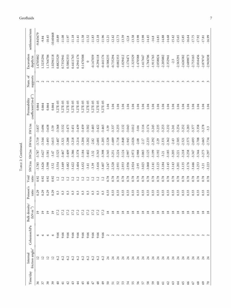
Table2:Con

tinu

ed.

Tim

e/day

Internal

friction

angle/°

Coh

esion/kP

aBulkdensity/

(kN·m

-3)

Poisson

’sratio

Void

ratio

SW3/m

SW2m

SW4/m

SW1/m

Permeability

coeffi

cient/(m

·d-1 )

Num

.of

supp

orts

Excavation

depth/m

settlement/mm

3612

619

0.29

0.92

-3.785

-3.787

-3.719

-3.837

0.864

21.4705882

-9.845679

3712

619

0.29

0.92

-3.626

-3.627

-3.544

-3.696

0.864

21.3235294

-9.84

3812

619

0.29

0.92

-3.598

-3.581

-3.493

-3.638

0.864

21.1764706

-10.45

3912

619

0.29

0.92

-3.52

-3.47

-3.615

-3.59

0.864

21.0294118

-10.60468

406.2

9.66

17.2

0.3

1.2

-3.554

-3.525

-3.407

-3.568

5.27E-05

20.8823529

-10.89

416.2

9.66

17.2

0.3

1.2

-3.449

-3.467

-3.321

-3.532

5.27E-05

20.7352941

-11.08

426.2

9.66

17.2

0.3

1.2

-3.482

-3.409

-3.288

-3.475

5.27E-05

20.5882353

-11.97

436.2

9.66

17.2

0.3

1.2

-3.422

-3.386

-3.218

-3.451

5.27E-05

20.4411765

-11.18

446.2

9.66

17.2

0.3

1.2

-3.404

-3.378

-3.214

-3.439

5.27E-05

20.2941176

-11.41

456.2

9.66

17.2

0.3

1.2

-3.432

-3.184

-3.204

-3.459

5.27E-05

20.1470588

-11.58

466.2

9.66

17.2

0.3

1.2

-3.41

-3.402

-3.202

-3.502

5.27E-05

20

-11.52

476.2

9.66

17.2

0.3

1.2

-3.39

-3.32

-2.82

-3.483

5.27E-05

2-0.147059

-11.83

486.2

9.66

17.2

0.3

1.2

-3.416

-3.343

-2.681

-3.422

5.27E-05

2-0.294118

-12.18

496.2

9.66

17.2

0.3

1.2

-3.407

-3.398

-1.205

-3.465

5.27E-05

2-0.441176

-11.96

5024

218

0.33

0.78

-3.247

-3.345

-2.528

-3.39

1.04

2-0.588235

-12.21

5124

218

0.33

0.78

-2.528

-3.251

-1.689

-3.337

1.04

2-0.735294

-12.42

5224

218

0.33

0.78

-2.931

-3.224

-1.718

-3.255

1.04

2-0.882353

-12.73

5324

218

0.33

0.78

-2.933

-3.124

-1.848

-3.132

1.04

2-1.029412

-13.59

5424

218

0.33

0.78

-2.936

-2.997

-1.945

-3.043

1.04

2-1.176471

-12.8

5524

218

0.33

0.78

-2.924

-2.972

-2.026

-3.012

1.04

2-1.323529

-13.58

5624

218

0.33

0.78

-2.95

-2.988

-2.08

-3.04

1.04

2-1.470588

-13.98

5724

218

0.33

0.78

-3.025

-3.065

-2.17

-3.116

1.04

2-1.617647

-13.98

5824

218

0.33

0.78

-3.068

-3.125

-2.233

-3.174

1.04

2-1.764706

-14.45

5924

218

0.33

0.78

-3.141

-3.199

-2.292

-3.245

1.04

2-1.911765

-14.8

6024

218

0.33

0.78

-3.125

-3.192

-2.29

-3.235

1.04

2-2.058824

-14.81

6124

218

0.33

0.78

-3.184

-3.21

-2.331

-3.253

1.04

2-2.205882

-14.88

6224

218

0.33

0.78

-3.145

-3.185

-2.362

-3.232

1.04

2-2.352941

-14.68

6324

218

0.33

0.78

-3.143

-3.205

-2.43

-3.241

1.04

3-2.5

-15.42

6424

218

0.33

0.78

-3.201

-3.221

-2.505

-3.254

1.04

3-2.563291

-15.65

6524

218

0.33

0.78

-3.135

-3.218

-2.521

-3.252

1.04

3-2.626582

-15.85

6624

218

0.33

0.78

-3.176

-3.258

-2.575

-3.283

1.04

3-2.689873

-16.64

6724

218

0.33

0.78

-3.446

-3.347

-2.693

-3.377

1.04

3-2.753165

-17.75

6824

218

0.33

0.78

-3.253

-3.344

-2.708

-3.358

1.04

3-2.816456

-17.92

6924

218

0.33

0.78

-3.21

-3.275

-2.665

-3.278

1.04

3-2.879747

-17.81

7024

218

0.33

0.78

-3.223

-3.297

-2.734

-3.3

1.04

3-2.943038

-16.99

7Geofluids

Page 8

Table2:Con

tinu

ed.

Tim

e/day

Internal

friction

angle/°

Coh

esion/kP

aBulkdensity/

(kN·m

-3)

Poisson

’sratio

Void

ratio

SW3/m

SW2m

SW4/m

SW1/m

Permeability

coeffi

cient/(m

·d-1 )

Num

.of

supp

orts

Excavation

depth/m

settlement/mm

7124

218

0.33

0.78

-3.244

-3.279

-2.748

-3.292

1.04

3-3.006329

-17.22

7224

218

0.33

0.78

-3.224

-3.192

-2.688

-3.284

1.04

3-3.06962

-16.94

7324

218

0.33

0.78

-3.229

-3.324

-2.798

-3.343

1.04

3-3.132911

-18.29

7424

218

0.33

0.78

-3.272

-3.328

-2.79

-3.381

1.04

3-3.196203

-19.54

7524

218

0.33

0.78

-3.239

-3.334

-2.669

-3.355

1.04

3-3.259494

-19.14

7624

218

0.33

0.78

-3.287

-3.268

-2.723

-3.262

1.04

3-3.322785

-20.49

7724

218

0.33

0.78

-3.185

-3.258

-2.758

-3.242

1.04

3-3.386076

-20.39

7824

218

0.33

0.78

-3.23

-3.296

-2.81

-3.25

1.04

3-3.449367

-19.16

7924

218

0.33

0.78

-3.195

-3.258

-2.833

-3.222

1.04

3-3.512658

-19.78

8024

218

0.33

0.78

-3.188

-3.232

-2.865

-3.22

1.04

3-3.575949

-20.52

8124

218

0.33

0.78

-3.237

-3.263

-2.894

-3.222

1.04

3-3.639241

-20.52

8224

218

0.33

0.78

-3.185

-3.263

-2.915

-3.233

1.04

3-3.702532

-19.2

8324

218

0.33

0.78

-3.214

-3.288

-2.952

-3.263

1.04

3-3.765823

-18.73

8424

218

0.33

0.78

-3.16

-3.336

-2.962

-3.248

1.04

3-3.829114

-20.28

8524

218

0.33

0.78

-3.215

-3.252

-2.973

-3.288

1.04

3-3.892405

-21.01

8624

218

0.33

0.78

-3.2

-3.275

-2.966

-3.284

1.04

3-3.955696

-22.01

8724

218

0.33

0.78

-3.433

-3.264

-2.887

-3.253

1.04

3-4.018987

-22.17

8824

218

0.33

0.78

-3.122

-3.223

-2.447

-3.178

1.04

3-4.082278

-22.31

8924

218

0.33

0.78

-3.082

-3.02

-2.377

-3.088

1.04

3-4.14557

-21.92

9024

218

0.33

0.78

-2.992

-3.055

-2.336

-3.1

1.04

3-4.208861

-23.36

9124

218

0.33

0.78

-2.92

-2.98

-2.33

-3.01

1.04

3-4.272152

-22.69

9224

218

0.33

0.78

-2.917

-2.928

-2.324

-2.902

1.04

3-4.335443

-23.4

9324

218

0.33

0.78

-2.92

-2.912

-2.341

-2.89

1.04

3-4.398734

-22.55

9424

218

0.33

0.78

-2.771

-2.778

-2.297

-2.748

1.04

3-4.462025

-23.65

9524

218

0.33

0.78

-3.043

-2.736

-2.231

-2.669

1.04

3-4.525316

-23.08

9624

218

0.33

0.78

-2.813

-2.712

-2.219

-2.629

1.04

3-4.588608

-23.34

9724

218

0.33

0.78

-2.853

-2.775

-2.267

-2.685

1.04

3-4.651899

-22.56

9824

218

0.33

0.78

-2.852

-2.788

-1.846

-2.718

1.04

3-4.71519

-23.17

9924

218

0.33

0.78

-2.877

-2.828

-2.026

-2.738

1.04

3-4.778481

-23.48

100

242

180.33

0.78

-2.91

-2.888

-2.17

-2.793

1.04

3-4.841772

-24.16

101

242

180.33

0.78

-2.894

-2.923

-2.188

-2.824

1.04

3-4.905063

-25.78

102

242

180.33

0.78

-2.896

-2.887

-2.224

-2.764

1.04

3-4.968354

-24.41

103

242

180.33

0.78

-2.833

-2.834

-2.167

-2.678

1.04

3-5.031646

-23.68

104

242

180.33

0.78

-2.938

-2.788

-2.112

-2.637

1.04

3-5.094937

-26.52

105

242

180.33

0.78

-2.861

-2.848

-2.197

-2.698

1.04

3-5.158228

-24.87

8 Geofluids

Page 9

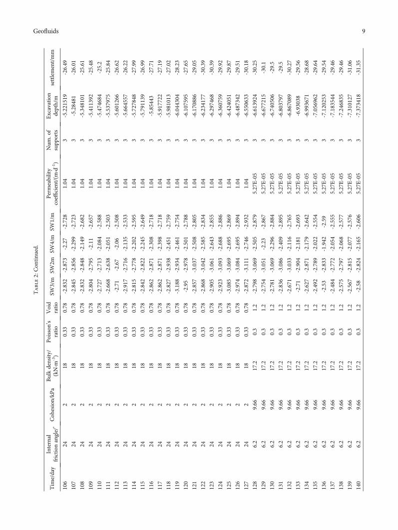
Table2:Con

tinu

ed.

Tim

e/day

Internal

friction

angle/°

Coh

esion/kP

aBulkdensity/

(kN·m

-3)

Poisson

’sratio

Void

ratio

SW3/m

SW2m

SW4/m

SW1/m

Permeability

coeffi

cient/(m

·d-1 )

Num

.of

supp

orts

Excavation

depth/m

settlement/mm

106

242

180.33

0.78

-2.832

-2.873

-2.27

-2.728

1.04

3-5.221519

-26.49

107

242

180.33

0.78

-2.845

-2.856

-2.299

-2.723

1.04

3-5.28481

-26.01

108

242

180.33

0.78

-2.832

-2.848

-2.149

-2.682

1.04

3-5.348101

-25.61

109

242

180.33

0.78

-2.804

-2.795

-2.11

-2.657

1.04

3-5.411392

-25.48

110

242

180.33

0.78

-2.727

-2.713

-2.084

-2.588

1.04

3-5.474684

-25.2

111

242

180.33

0.78

-2.668

-2.638

-2.051

-2.503

1.04

3-5.537975

-25.84

112

242

180.33

0.78

-2.71

-2.67

-2.06

-2.508

1.04

3-5.601266

-26.62

113

242

180.33

0.78

-2.917

-2.716

-2.135

-2.533

1.04

3-5.664557

-26.22

114

242

180.33

0.78

-2.815

-2.778

-2.202

-2.595

1.04

3-5.727848

-27.99

115

242

180.33

0.78

-2.842

-2.822

-2.245

-2.649

1.04

3-5.791139

-26.99

116

242

180.33

0.78

-2.862

-2.871

-2.308

-2.718

1.04

3-5.85443

-27.71

117

242

180.33

0.78

-2.862

-2.871

-2.398

-2.718

1.04

3-5.917722

-27.19

118

242

180.33

0.78

-2.827

-2.938

-2.451

-2.759

1.04

3-5.981013

-27.02

119

242

180.33

0.78

-3.188

-2.934

-2.461

-2.754

1.04

3-6.044304

-28.23

120

242

180.33

0.78

-2.95

-2.978

-2.501

-2.788

1.04

3-6.107595

-27.65

121

242

180.33

0.78

-2.857

-3.037

-2.508

-2.805

1.04

3-6.170886

-29.05

122

242

180.33

0.78

-2.868

-3.042

-2.585

-2.834

1.04

3-6.234177

-30.39

123

242

180.33

0.78

-2.905

-3.061

-2.643

-2.855

1.04

3-6.297468

-30.39

124

242

180.33

0.78

-2.923

-3.093

-2.688

-2.886

1.04

3-6.360759

-29.92

125

242

180.33

0.78

-3.085

-3.069

-2.695

-2.869

1.04

3-6.424051

-29.87

126

242

180.33

0.78

-2.974

-3.084

-2.695

-2.894

1.04

3-6.487342

-29.51

127

242

180.33

0.78

-2.872

-3.111

-2.746

-2.932

1.04

3-6.550633

-30.18

128

6.2

9.66

17.2

0.3

1.2

-2.798

-3.069

-2.505

-2.879

5.27E-05

3-6.613924

-30.25

129

6.2

9.66

17.2

0.3

1.2

-2.754

-3.051

-2.23

-2.867

5.27E-05

3-6.677215

-30.1

130

6.2

9.66

17.2

0.3

1.2

-2.781

-3.069

-2.296

-2.884

5.27E-05

3-6.740506

-29.5

131

6.2

9.66

17.2

0.3

1.2

-2.836

-3.086

-2.409

-2.895

5.27E-05

3-6.803797

-29.5

132

6.2

9.66

17.2

0.3

1.2

-2.671

-3.033

-2.116

-2.765

5.27E-05

3-6.867089

-30.27

133

6.2

9.66

17.2

0.3

1.2

-2.71

-2.904

-2.181

-2.693

5.27E-05

3-6.93038

-29.56

134

6.2

9.66

17.2

0.3

1.2

-2.627

-2.871

-2.179

-2.642

5.27E-05

3-6.993671

-28.68

135

6.2

9.66

17.2

0.3

1.2

-2.492

-2.789

-2.022

-2.554

5.27E-05

3-7.056962

-29.64

136

6.2

9.66

17.2

0.3

1.2

-2.53

-2.833

-1.942

-2.59

5.27E-05

3-7.120253

-29.54

137

6.2

9.66

17.2

0.3

1.2

-2.484

-2.772

-2.054

-2.555

5.27E-05

3-7.183544

-29.46

138

6.2

9.66

17.2

0.3

1.2

-2.575

-2.797

-2.068

-2.577

5.27E-05

3-7.246835

-29.46

139

6.2

9.66

17.2

0.3

1.2

-2.567

-2.815

-2.077

-2.576

5.27E-05

3-7.310127

-31.06

140

6.2

9.66

17.2

0.3

1.2

-2.58

-2.824

-2.165

-2.606

5.27E-05

3-7.373418

-31.35

9Geofluids

Page 10

Table2:Con

tinu

ed.

Tim

e/day

Internal

friction

angle/°

Coh

esion/kP

aBulkdensity/

(kN·m

-3)

Poisson

’sratio

Void

ratio

SW3/m

SW2m

SW4/m

SW1/m

Permeability

coeffi

cient/(m

·d-1 )

Num

.of

supp

orts

Excavation

depth/m

settlement/mm

141

6.2

9.66

17.2

0.3

1.2

-2.604

-2.833

-2.244

-2.633

5.27E-05

3-7.436709

-31.35

142

6.2

9.66

17.2

0.3

1.2

-2.621

-2.849

-2.292

-2.625

5.27E-05

4-7.5

-31.35

143

6.2

9.66

17.2

0.3

1.2

-3.029

-2.85

-2.325

-2.617

5.27E-05

4-7.857143

-31.35

144

6.2

9.66

17.2

0.3

1.2

-2.618

-2.83

-2.221

-2.59

5.27E-05

4-8.214286

-31.35

145

6.2

9.66

17.2

0.3

1.2

-2.559

-2.784

-2.074

-2.516

5.27E-05

4-8.571429

-31.35

146

6.2

9.66

17.2

0.3

1.2

-2.427

-2.624

-1.949

-2.386

5.27E-05

4-8.928571

-31.35

147

6.2

9.66

17.2

0.3

1.2

-2.347

-2.539

-1.896

-2.27

5.27E-05

4-9.285714

-33.52

148

6.2

9.66

17.2

0.3

1.2

-2.334

-2.457

-1.901

-2.242

5.27E-05

4-9.642857

-31.52

149

6.2

9.66

17.2

0.3

1.2

-2.41

-2.449

-1.915

-2.19

5.27E-05

4-10

-31.31

150

6.2

9.66

17.2

0.3

1.2

-2.435

-2.532

-2.038

-2.279

5.27E-05

4-10.35714

-32.11

151

6.2

9.66

17.2

0.3

1.2

-2.461

-2.628

-2.085

-2.346

5.27E-05

4-10.71429

-32.58

152

6.2

9.66

17.2

0.3

1.2

-2.198

-2.677

-1.978

-2.4

5.27E-05

4-11.07143

-31.49

153

6.2

9.66

17.2

0.3

1.2

-2.57

-2.722

-2.021

-2.449

5.27E-05

4-11.42857

-30.98

154

6.2

9.66

17.2

0.3

1.2

-2.576

-2.728

-2.167

-2.456

5.27E-05

4-11.78571

-32.13

155

6.2

9.66

17.2

0.3

1.2

-2.688

-2.764

-2.282

-2.477

5.27E-05

4-12.14286

-33.2

156

6.2

9.66

17.2

0.3

1.2

-2.742

-2.814

-2.362

-2.514

5.27E-05

5-12.5

-33.2

157

6.2

9.66

17.2

0.3

1.2

-2.016

-2.854

-2.424

-2.562

5.27E-05

5-12.71429

-34.8

158

6.2

9.66

17.2

0.3

1.2

-2.407

-2.753

-2.143

-2.457

5.27E-05

5-12.92857

-34.8

159

6.2

9.66

17.2

0.3

1.2

-2.302

-2.724

-2.194

-2.422

5.27E-05

5-13.14286

-34.74

160

6.2

9.66

17.2

0.3

1.2

-2.477

-2.68

-2.163

-2.398

5.27E-05

5-13.35714

-33.06

161

6.2

9.66

17.2

0.3

1.2

-2.437

-2.713

-2.207

-2.434

5.27E-05

5-13.57143

-34.15

162

6.2

9.66

17.2

0.3

1.2

-2.762

-2.743

-2.271

-2.454

5.27E-05

5-13.78571

-34.57

163

6.2

9.66

17.2

0.3

1.2

-2.723

-2.763

-2.124

-2.482

5.27E-05

5-14

-34.37

164

6.2

9.66

17.2

0.3

1.2

-2.607

-2.809

-2.272

-2.496

5.27E-05

5-14.21429

-34.33

165

6.2

9.66

17.2

0.3

1.2

-2.771

-2.871

-2.262

-2.526

5.27E-05

5-14.42857

-33.68

166

6.2

9.66

17.2

0.3

1.2

-2.493

-2.778

-2.137

-2.47

5.27E-05

5-14.64286

-34.65

167

6.2

9.66

17.2

0.3

1.2

-2.512

-2.74

-2.084

-2.541

5.27E-05

5-14.85714

-35.62

168

6.2

9.66

17.2

0.3

1.2

-3.163

-2.742

-2.154

-6.692

5.27E-05

5-15.07143

-36.95

169

6.2

9.66

17.2

0.3

1.2

-2.962

-2.804

-2.345

-3.86

5.27E-05

5-15.28571

-36.93

170

6.2

9.66

17.2

0.3

1.2

-3.33

-2.845

-2.424

-4.934

5.27E-05

5-15.5

-37.14

171

6.2

9.66

17.2

0.3

1.2

-3.326

-2.848

-2.428

-4.928

5.27E-05

5-15.71429

-37.19

172

6.2

9.66

17.2

0.3

1.2

-3.15

-2.842

-2.428

-4.645

5.27E-05

5-15.92857

-37.5

173

242

180.33

0.78

-3.092

-2.843

-2.422

-4.055

1.04

5-16.14286

-37.86

174

242

180.33

0.78

-2.495

-2.742

-2.082

-3.543

1.04

5-16.35714

-37.8

175

242

180.33

0.78

-2.57

-2.68

-2.071

-2.84

1.04

5-16.57143

-37.42

10 Geofluids

Page 11

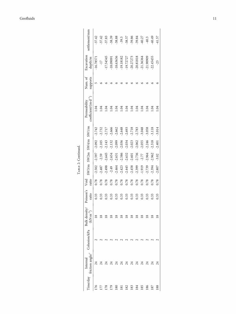
Table2:Con

tinu

ed.

Tim

e/day

Internal

friction

angle/°

Coh

esion/kP

aBulkdensity/

(kN·m

-3)

Poisson

’sratio

Void

ratio

SW3/m

SW2m

SW4/m

SW1/m

Permeability

coeffi

cient/(m

·d-1 )

Num

.of

supp

orts

Excavation

depth/m

settlement/mm

176

242

180.33

0.78

-2.502

-2.597

-2.092

-2.742

1.04

5-16.78571

-37.42

177

242

180.33

0.78

-2.487

-2.59

-2.105

-2.732

1.04

6-17

-37.42

178

242

180.33

0.78

-2.498

-2.645

-2.143

-2.717

1.04

6-17.54545

-37.83

179

242

180.33

0.78

-2.49

-2.654

-2.132

-2.666

1.04

6-18.09091

-38.39

180

242

180.33

0.78

-2.464

-2.631

-2.099

-2.662

1.04

6-18.63636

-38.88

181

242

180.33

0.78

-2.423

-2.586

-2.036

-2.648

1.04

6-19.18182

-39.3

182

242

180.33

0.78

-2.445

-2.632

-2.034

-2.693

1.04

6-19.72727

-38.57

183

242

180.33

0.78

-2.458

-2.601

-2.023

-2.718

1.04

6-20.27273

-39.86

184

242

180.33

0.78

-2.399

-2.736

-2.062

-2.783

1.04

6-20.81818

-39.84

185

242

180.33

0.78

-1.919

-2.77

-2.055

-3.048

1.04

6-21.36364

-40.27

186

242

180.33

0.78

-2.739

-2.964

-2.246

-3.058

1.04

6-21.90909

-40.3

187

242

180.33

0.78

-2.394

-2.962

-2.318

-3.118

1.04

6-22.45455

-40.49

188

242

180.33

0.78

-2.807

-3.02

-2.401

-3.014

1.04

6-23

-41.57

11Geofluids

Page 12

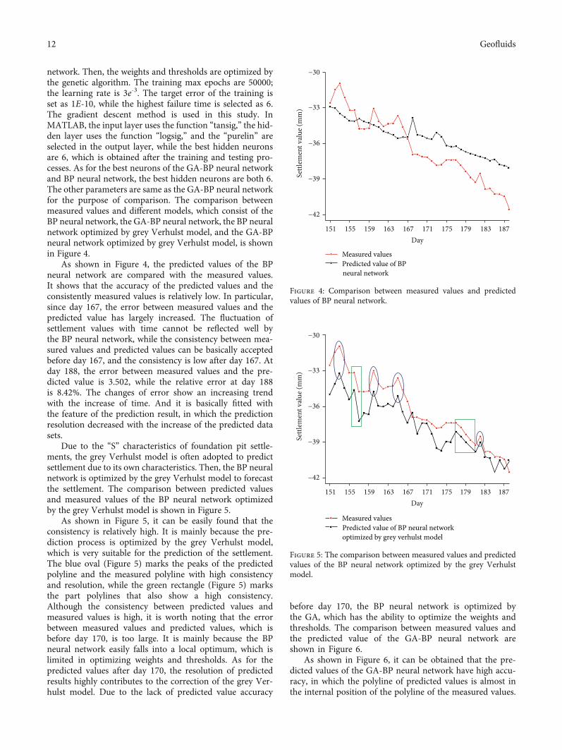
network. Then, the weights and thresholds are optimized bythe genetic algorithm. The training max epochs are 50000;the learning rate is 3e-3. The target error of the training isset as 1E-10, while the highest failure time is selected as 6.The gradient descent method is used in this study. InMATLAB, the input layer uses the function “tansig,” the hid-den layer uses the function “logsig,” and the “purelin” areselected in the output layer, while the best hidden neuronsare 6, which is obtained after the training and testing pro-cesses. As for the best neurons of the GA-BP neural networkand BP neural network, the best hidden neurons are both 6.The other parameters are same as the GA-BP neural networkfor the purpose of comparison. The comparison betweenmeasured values and different models, which consist of theBP neural network, the GA-BP neural network, the BP neuralnetwork optimized by grey Verhulst model, and the GA-BPneural network optimized by grey Verhulst model, is shownin Figure 4.

As shown in Figure 4, the predicted values of the BPneural network are compared with the measured values.It shows that the accuracy of the predicted values and theconsistently measured values is relatively low. In particular,since day 167, the error between measured values and thepredicted value has largely increased. The fluctuation ofsettlement values with time cannot be reflected well bythe BP neural network, while the consistency between mea-sured values and predicted values can be basically acceptedbefore day 167, and the consistency is low after day 167. Atday 188, the error between measured values and the pre-dicted value is 3.502, while the relative error at day 188is 8.42%. The changes of error show an increasing trendwith the increase of time. And it is basically fitted withthe feature of the prediction result, in which the predictionresolution decreased with the increase of the predicted datasets.

Due to the “S” characteristics of foundation pit settle-ments, the grey Verhulst model is often adopted to predictsettlement due to its own characteristics. Then, the BP neuralnetwork is optimized by the grey Verhulst model to forecastthe settlement. The comparison between predicted valuesand measured values of the BP neural network optimizedby the grey Verhulst model is shown in Figure 5.

As shown in Figure 5, it can be easily found that theconsistency is relatively high. It is mainly because the pre-diction process is optimized by the grey Verhulst model,which is very suitable for the prediction of the settlement.The blue oval (Figure 5) marks the peaks of the predictedpolyline and the measured polyline with high consistencyand resolution, while the green rectangle (Figure 5) marksthe part polylines that also show a high consistency.Although the consistency between predicted values andmeasured values is high, it is worth noting that the errorbetween measured values and predicted values, which isbefore day 170, is too large. It is mainly because the BPneural network easily falls into a local optimum, which islimited in optimizing weights and thresholds. As for thepredicted values after day 170, the resolution of predictedresults highly contributes to the correction of the grey Ver-hulst model. Due to the lack of predicted value accuracy

before day 170, the BP neural network is optimized bythe GA, which has the ability to optimize the weights andthresholds. The comparison between measured values andthe predicted value of the GA-BP neural network areshown in Figure 6.

As shown in Figure 6, it can be obtained that the pre-dicted values of the GA-BP neural network have high accu-racy, in which the polyline of predicted values is almost inthe internal position of the polyline of the measured values.

−30

−33

−36

−39Settl

emen

t val

ue (m

m)

−42

151 155 159 163 167 171Day

175 179 183 187

Measured valuesPredicted value of BPneural network

Figure 4: Comparison between measured values and predictedvalues of BP neural network.

−30

−33

−36

−39Settl

emen

t val

ue (m

m)

−42

151 155 159 163 167 171Day

175 179 183 187

Measured valuesPredicted value of BP neural networkoptimized by grey verhulst model

Figure 5: The comparison between measured values and predictedvalues of the BP neural network optimized by the grey Verhulstmodel.

12 Geofluids

Page 13

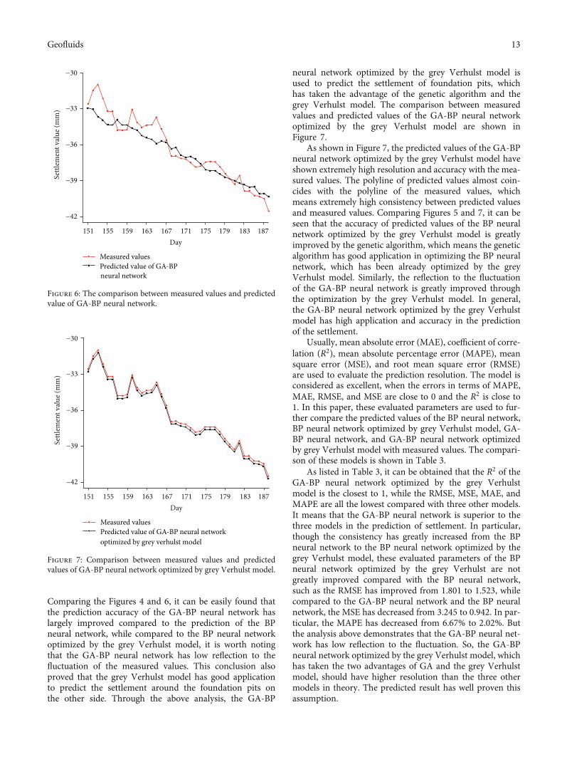
Comparing the Figures 4 and 6, it can be easily found thatthe prediction accuracy of the GA-BP neural network haslargely improved compared to the prediction of the BPneural network, while compared to the BP neural networkoptimized by the grey Verhulst model, it is worth notingthat the GA-BP neural network has low reflection to thefluctuation of the measured values. This conclusion alsoproved that the grey Verhulst model has good applicationto predict the settlement around the foundation pits onthe other side. Through the above analysis, the GA-BP

neural network optimized by the grey Verhulst model isused to predict the settlement of foundation pits, whichhas taken the advantage of the genetic algorithm and thegrey Verhulst model. The comparison between measuredvalues and predicted values of the GA-BP neural networkoptimized by the grey Verhulst model are shown inFigure 7.

As shown in Figure 7, the predicted values of the GA-BPneural network optimized by the grey Verhulst model haveshown extremely high resolution and accuracy with the mea-sured values. The polyline of predicted values almost coin-cides with the polyline of the measured values, whichmeans extremely high consistency between predicted valuesand measured values. Comparing Figures 5 and 7, it can beseen that the accuracy of predicted values of the BP neuralnetwork optimized by the grey Verhulst model is greatlyimproved by the genetic algorithm, which means the geneticalgorithm has good application in optimizing the BP neuralnetwork, which has been already optimized by the greyVerhulst model. Similarly, the reflection to the fluctuationof the GA-BP neural network is greatly improved throughthe optimization by the grey Verhulst model. In general,the GA-BP neural network optimized by the grey Verhulstmodel has high application and accuracy in the predictionof the settlement.

Usually, mean absolute error (MAE), coefficient of corre-lation (R2), mean absolute percentage error (MAPE), meansquare error (MSE), and root mean square error (RMSE)are used to evaluate the prediction resolution. The model isconsidered as excellent, when the errors in terms of MAPE,MAE, RMSE, and MSE are close to 0 and the R2 is close to1. In this paper, these evaluated parameters are used to fur-ther compare the predicted values of the BP neural network,BP neural network optimized by grey Verhulst model, GA-BP neural network, and GA-BP neural network optimizedby grey Verhulst model with measured values. The compari-son of these models is shown in Table 3.

As listed in Table 3, it can be obtained that the R2 of theGA-BP neural network optimized by the grey Verhulstmodel is the closest to 1, while the RMSE, MSE, MAE, andMAPE are all the lowest compared with three other models.It means that the GA-BP neural network is superior to thethree models in the prediction of settlement. In particular,though the consistency has greatly increased from the BPneural network to the BP neural network optimized by thegrey Verhulst model, these evaluated parameters of the BPneural network optimized by the grey Verhulst are notgreatly improved compared with the BP neural network,such as the RMSE has improved from 1.801 to 1.523, whilecompared to the GA-BP neural network and the BP neuralnetwork, the MSE has decreased from 3.245 to 0.942. In par-ticular, the MAPE has decreased from 6.67% to 2.02%. Butthe analysis above demonstrates that the GA-BP neural net-work has low reflection to the fluctuation. So, the GA-BPneural network optimized by the grey Verhulst model, whichhas taken the two advantages of GA and the grey Verhulstmodel, should have higher resolution than the three othermodels in theory. The predicted result has well proven thisassumption.

−30

−33

−36

−39Settl

emen

t val

ue (m

m)

−42

151 155 159 163 167 171Day

175 179 183 187

Measured valuesPredicted value of GA-BPneural network

Figure 6: The comparison between measured values and predictedvalue of GA-BP neural network.

−30

−33

−36

−39Settl

emen

t val

ue (m

m)

−42

151 155 159 163 167 171Day

175 179 183 187

Measured valuesPredicted value of GA-BP neural networkoptimized by grey verhulst model

Figure 7: Comparison between measured values and predictedvalues of GA-BP neural network optimized by grey Verhulst model.

13Geofluids

Page 14

4. Summary and Conclusions

Because of the influence of many factors, settlement aroundthe foundation pit is hard to predict. In this paper, the settle-ment of D4 is studied due to a large settlement value andbeing close to the bridge pier of a highway. The internal fric-tion angle, cohesion, bulk density, Poisson’s ratio, void ratio,water level changes, permeability coefficient, number of sup-ports, and excavation depth, which influence the settlementaround foundation pits, are adopted as the input parametersof the prediction model. Since the supporting time is pre-cisely recorded, the correspondence between the real-timeexcavation depth and the excavation time can be obtained.Then, the first 150 data sets are used to establish the model,and the last 38 data sets are taken to verify the accuracy ofthe established model. To obtain a suitable model, the BPneural network, GA-BP neural network, BP neural networkoptimized by grey Verhulst model, and GA-BP neural net-work optimized by grey Verhulst model are used to predictthe settlement of foundation pits, and the comparisons aredetailed analysed. The following conclusions can beadvanced from this paper:

(1) Due to insufficient consideration of influencing fac-tors in previous studies, the internal friction angle,cohesion, bulk density, Poisson’s ratio, void ratio,water level changes, permeability coefficient, numberof supports, and excavation depth are taken into con-sideration in this study. Through the analysis of theprediction results, the selection of these input param-eters has high guiding significance for the predictionsettlement around foundation pits

(2) This paper proposed a new model, which is com-bined with the BP neural, genetic algorithm, and greyVerhulst models, to predict the settlement of a certainday or excavation to a certain depth in a long periodof time in the future, which has guiding significancefor engineering construction

(3) The predicted values of the BP neural network, BPneural network optimized by the grey Verhulstmodel, GA-BP neural network, and GA-BP neuralnetwork optimized by the grey Verhulst model arecompared with measured values. The results showthat the grey Verhulst model can greatly improvethe consistency between predicted values and mea-sured values, while the accuracy of the early stage islow. It is mainly because the BP neural network easilyfalls into a local optimum. The genetic algorithm

(GA), which can largely improve the accuracy of pre-dicted values, has low reflection to the fluctuation ofmeasured values. The GA-BP neural network opti-mized by the grey Verhulst model, which takes theadvantages of the genetic algorithm (GA) and greyVerhulst model, has extremely high consistency andaccuracy with measured values. The results of RMSE,MAE, R2, and MSE further prove the conclusion

Data Availability

The experimental data used to support the findings of thisstudy are included within the article.

Conflicts of Interest

The authors declare that there are no conflicts of interestregarding the publication of this paper.

References

[1] Y. He, B. B. Li, K. N. Zhang, Z. Li, Y. G. Chen, and W. M. Ye,“Experimental and numerical study on heavy metal contami-nant migration and retention behavior of engineered barrierin tailings pond,” Environmental Pollution, vol. 252, Part B,pp. 1010–1018, 2019.

[2] C. M. Zhang, “Applications of soil nailed wall in foundation pitsupport,” Applied Mechanics and Materials, vol. 353-356,pp. 969–973, 2013.

[3] X. Zhang, Y. Wu, E. Zhai, and P. Ye, “Coupling analysis of theheat-water dynamics and frozen depth in a seasonally frozenzone,” Journal of Hydrology, vol. 593, article 125603, 2020.

[4] J. Du, G. Zheng, B. Liu, N. J. Jiang, and J. Hu, “Triaxial behav-ior of cement-stabilized organic matter–disseminated sand,”Acta Geotechnica, vol. 16, no. 1, pp. 211–220, 2021.

[5] C. Zhu, X. Xu,W. Liu, F. Xiong, and X. Liu, “Softening damageanalysis of gypsum rock with water immersion time based onlaboratory experiment,” IEEE Access, vol. 7, pp. 125575–125585, 2019.

[6] C. Liu, Y. Wang, X. Zhang, and L. Du, “Rock brittleness eval-uation method based on the complete stress-strain curve,”Frattura ed Integrità Strutturale, vol. 13, no. 49, pp. 557–567,2019.

[7] C. Liu, X. Hu, R. Yao et al., “Assessment of soil thermal con-ductivity based on BPNN optimized by genetic algorithm,”Advances in Civil Engineering, vol. 2020, Article ID 6631666,10 pages, 2020.

[8] W. Wang, L.-q. Li, W.-y. Xu, Q.-x. Meng, and J. Lu, “Creepfailure mode and criterion of Xiangjiaba sandstone,” Journalof Central South University, vol. 19, no. 12, pp. 3572–3581,2012.

Table 3: Calculation results of performance indexes for these models.

Models RMSE (mm) MSE (mm2) MAE (mm) MAPE (%) R2

BP neural network 1.801 3.245 1.592 6.67 0.570

BP neural network optimized by grey Verhulst model 1.523 2.319 1.348 8.84 0.692

GA-BP neural network 0.971 0.942 0.780 2.02 0.720

GA-BP neural network optimized by grey Verhulst model 0.221 0.049 0.221 1.59 0.994

14 Geofluids

Page 15

[9] L. L. Yang, W. Y. Xu, Q. X. Meng, and R. B. Wang, “Investiga-tion on jointed rock strength based on fractal theory,” Journalof Central South University, vol. 24, no. 7, pp. 1619–1626, 2017.

[10] Y. Wu, Y. Xu, X. Zhang et al., “Experimental study on vacuumpreloading consolidation of landfill sludge conditioned byFenton’s reagent under varying filter pore size,” Geotextilesand Geomembranes, vol. 49, no. 1, pp. 109–121, 2021.

[11] C. Zhu, M. He, M. Karakus, X. Cui, and Z. Tao, “Investigatingtoppling failure mechanism of anti-dip layered slope due toexcavation by physical modelling,” Rock Mechanics and RockEngineering, vol. 53, pp. 5029–5050, 2020.

[12] W. Zhang, R. Zhang, C. Wu et al., “State-of-the-art review ofsoft computing applications in underground excavations,”Geoscience Frontiers, vol. 11, no. 4, pp. 1095–1106, 2020.

[13] Z. Li, S. G. Liu, W. T. Ren, J. J. Fang, Q. H. Zhu, and Z. L. Dun,“Multiscale laboratory study and numerical analysis of water-weakening effect on shale,” Advances in Materials Scienceand Engineering, vol. 2020, Article ID 5263431, 14 pages, 2020.

[14] Y. Wang, B. Zhang, S. H. Gao, and C. H. Li, “Investigation onthe effect of freeze-thaw on fracture mode classification inmarble subjected to multi-level cyclic loads,” Theoretical andApplied Fracture Mechanics, vol. 111, article 102847, 2021.

[15] Y. Yao, J. Huang, N. Wang, T. Luo, and L. Han, “Predictionmethod of creep settlement considering abrupt factors,”Transportation Geotechnics, vol. 22, article 100304, 2019.

[16] Y. Tan and D. Wang, “Characteristics of a large-scale deepfoundation pit excavated by the central-island technique inShanghai soft clay. II: top-down construction of the peripheralrectangular pit,” Journal of Geotechnical and Geoenvironmen-tal Engineering, vol. 139, no. 11, pp. 1894–1910, 2013.

[17] Y. Tan, W.-Z. Jiang, H.-S. Rui, Y. Lu, and D.-L. Wang, “Foren-sic geotechnical analyses on the 2009 building-overturningaccident in Shanghai, China: beyond common recognitions,”Journal of Geotechnical and Geoenvironmental Engineering,vol. 146, no. 7, article 05020005, 2020.

[18] Y. Tan and D. Wang, “Characteristics of a large-scale deepfoundation pit excavated by the central-island technique inShanghai soft clay. I: bottom-up construction of the centralcylindrical shaft,” Journal of Geotechnical and Geoenviron-mental Engineering, vol. 139, no. 11, pp. 1875–1893, 2013.

[19] Q. Xu, H. Zhu, X. Ma et al., “A case history of shield tunnelcrossing through group pile foundation of a road bridge withpile underpinning technologies in Shanghai,” Tunnelling andUnderground Space Technology, vol. 45, pp. 20–33, 2015.

[20] Q. Meng, H. Wang, M. Cai, W. Xu, X. Zhuang, andT. Rabczuk, “Three-dimensional mesoscale computationalmodeling of soil-rock mixtures with concave particles,” Engi-neering Geology, vol. 277, article 105802, 2020.

[21] Z. Tao, C. Zhu, M. He, and M. Karakus, “A physical modeling-based study on the control mechanisms of negative Poisson'sratio anchor cable on the stratified toppling deformation ofanti-inclined slopes,” International Journal of Rock Mechanicsand Mining Sciences, vol. 138, article 104632, 2021.

[22] Q. X. Meng, H. L. Wang, W. Y. Xu, and Q. Zhang, “A couplingmethod incorporating digital image processing and discreteelement method for modeling of geomaterials,” EngineeringComputations, vol. 35, no. 1, pp. 411–431, 2018.

[23] Z. F. Wang, S. L. Shen, W. C. Cheng, and Y. S. Xu, “Ground fis-sures in Xi’an and measures to prevent damage to the metrotunnel system due to geohazards,” Environmental Earth Sci-ences, vol. 75, no. 6, article 511, 2016.

[24] X. Gao, W.-p. Tian, and Z. Zhang, “Analysis of deformationcharacteristics of foundation-pit excavation and circular wall,”Sustainability, vol. 12, no. 8, article 3164, 2020.

[25] Y. Zhou and Y. Zhu, “Interaction between pile-anchor sup-porting structure and soil in deep excavation,” Journal of Rockand Soil Mechanics, vol. 39, no. 9, pp. 3246–3252, 2018.

[26] Q. X. Meng, L. Yan, Y. L. Chen, and Q. Zhang, “Generation ofnumerical models of anisotropic columnar jointed rock massusing modified centroidal Voronoi diagrams,” Symmetry,vol. 10, no. 11, p. 618, 2018.

[27] A. Ismail and D. S. Jeng, “Modelling load–settlement behav-iour of piles using high-order neural network (HON-PILEmodel),” Engineering Applications of Artificial Intelligence,vol. 24, no. 5, pp. 813–821, 2011.

[28] A. Ghorbani and M. Firouzi Niavol, “Evaluation of inducedsettlements of piled rafts in the coupled static-dynamic loadsusing neural networks and evolutionary polynomial regres-sion,” Applied Computational Intelligence and Soft Computing,vol. 2017, Article ID 7487438, 23 pages, 2017.

[29] Y. Lv, T. Liu, J. Ma, S. Wei, and C. Gao, “Study on settlementprediction model of deep foundation pit in sand and pebblestrata based on grey theory and BP neural network,” ArabianJournal of Geosciences, vol. 13, no. 23, pp. 1–13, 2020.

[30] H. T. Eid and A. A. Shehada, “Estimating the elastic settlementof piled foundations on rock,” International Journal of Geome-chanics, vol. 15, no. 3, article 04014059, 2015.

[31] C. Xu, D. Yue, and C. Deng, “Hybrid GA/SIMPLS as alterna-tive regression model in dam deformation analysis,” Engineer-ing Applications of Artificial Intelligence, vol. 25, no. 3,pp. 468–475, 2012.

[32] X. Guo, S. Liu, L. Wu, Y. Gao, and Y. Yang, “A multi-variablegrey model with a self-memory component and its applicationon engineering prediction,” Engineering Applications of Artifi-cial Intelligence, vol. 42, pp. 82–93, 2015.

[33] M. A. Shahin, “Load–settlement modeling of axially loadeddrilled shafts using CPT-based recurrent neural networks,”International Journal of Geomechanics, vol. 14, no. 6, article06014012, 2014.

[34] J. P. Doherty, S. Gourvenec, and F. M. Gaone, “Insights from ashallow foundation load-settlement prediction exercise,” Com-puters and Geotechnics, vol. 93, pp. 269–279, 2018.

[35] F. P. Nejad and M. B. Jaksa, “Load-settlement behavior model-ing of single piles using artificial neural networks and CPTdata,” Computers and Geotechnics, vol. 89, pp. 9–21, 2017.

[36] M. Cao, L. X. Pan, Y. F. Gao et al., “Neural network ensemble-based parameter sensitivity analysis in civil engineering sys-tems,” Neural Computing and Applications, vol. 28, no. 7,pp. 1583–1590, 2017.

[37] J. Su, Y. Xia, Y. Xu, X. Zhao, and Q. Zhang, “Settlement mon-itoring of a supertall building using the Kalman filtering tech-nique and forward construction stage analysis,” Advances inStructural Engineering, vol. 17, no. 6, pp. 881–893, 2014.

[38] W. Dai, N. Liu, R. Santerre, and J. Pan, “Dam deformationmonitoring data analysis using space-time Kalman filter,”International Journal of Geo-Information, vol. 5, no. 12,p. 236, 2016.

[39] L. Zhang, X. Wu, W. Ji, and S. M. AbouRizk, “Intelligentapproach to estimation of tunnel-induced ground settlementusing wavelet packet and support vector machines,” Journalof Computing in Civil Engineering, vol. 31, no. 2, article04016053, 2017.

15Geofluids

Page 16

[40] C. Zhang, J.-z. Li, and H. Yong, “Application of optimized greydiscrete Verhulst–BP neural network model in settlement pre-diction of foundation pit,” Environmental Earth Sciences,vol. 78, no. 15, article 441, 2019.

[41] M. Guoxiong and Zai, “Proof and application of s-shapesettlement-time curve for linear or nearly linear loadings,”China Civil Engineering Journal, vol. 38, pp. 69–72, 2005.

[42] Wilun and Zenon, Soil Mechanics in Foundation Engineering:v.2: Theory and Practice, John Wiley, 1972.

[43] L. Tang and Y. Lu, “Study of the grey Verhulst model based onthe weighted least square method,” Physica A: StatisticalMechanics and its Applications, vol. 545, article 123615, 2020.

[44] H. Liu, W. Guo, C. Zhang, and H. Yang, “Research on the greyVerhulst model based on particle swarm optimization andMarkov chain to predict the settlement of high fill subgradein Xiangli expressway,” Mathematical Problems in Engineer-ing, vol. 2019, Article ID 1878296, 10 pages, 2019.

[45] B. Zeng, X. Ma, and M. Zhou, “A new-structure grey Verhulstmodel for China’s tight gas production forecasting,” AppliedSoft Computing, vol. 96, article 106600, 2020.

[46] Q. Ma, S. Liu, X. Fan, C. Chai, Y. Wang, and K. Yang, “A timeseries prediction model of foundation pit deformation basedon empirical wavelet transform and NARX network,” Mathe-matics, vol. 8, no. 9, article 1535, 2020.

[47] T. Niu, L. Zhang, S. Wei, B. Zhang, and B. Zhang, “Study on acombined prediction method based on BP neural network andimproved Verhulst model,” Systems Science & Control Engi-neering, vol. 7, no. 3, pp. 36–42, 2019.

[48] J. Wang, Y. Gao, and J. Jin, “Influence of sample length on grayfuzzy prediction performance,” Journal of Intelligent & FuzzySystems, vol. 38, no. 6, pp. 6745–6754, 2020.

[49] I. A. Basheer andM. Hajmeer, “Artificial neural networks: fun-damentals, computing, design, and application,” Journal ofMicrobiological Methods, vol. 43, no. 1, pp. 3–31, 2000.

[50] H. Peng, H. Wu, J. Wang, and T. Dede, “Research on the pre-diction of the water demand of construction engineering basedon the BP neural network,” Advances in Civil Engineering,vol. 2020, Article ID 8868817, 11 pages, 2020.

[51] S. M. Bateni, D.-S. Jeng, and S. M. Naeini, “Estimating soilthermal properties from sequences of land surface temperatureusing hybrid genetic algorithm–finite difference method,”Engineering Applications of Artificial Intelligence, vol. 25,no. 7, pp. 1425–1436, 2012.

[52] V. Gitifar, A. Abbasi, P. Setoodeh, M. Poursadegh,Z. Sahebnazar, and A. Alamdari, “Modeling and analysis ofthe thermal conductivities of air saturated sandstone, quartzand limestone using computational intelligence,” Interna-tional Journal of Thermal Sciences, vol. 83, pp. 45–55, 2014.

[53] J. R. Sampson, “Adaptation in natural and artificial systems,”in Society for Industrial and Applied Mathematics, J. H. Hol-land, Ed., SIAM Review, 1976.

[54] D. E. Goldberg and J. H. Holland, Genetic Algorithms andMachine Learning, vol. 3, pp. 95–99, Machine Learning, 1988.

[55] Y. Erzin and T. O. Gul, “The use of neural networks for theprediction of the settlement of one-way footings on cohesion-less soils based on standard penetration test,” Neural Comput-ing and Applications, vol. 24, no. 3-4, pp. 891–900, 2014.

[56] S. Freitag, B. Cao, J. Ninić, and G. Meschke, “Recurrent neuralnetworks and proper orthogonal decomposition with intervaldata for real-time predictions of mechanised tunnelling pro-cesses,” Computers & Structures, vol. 207, pp. 258–273, 2018.

[57] Z. W. Ji, B. Wang, S. P. Deng, and Z. H. You, “Predictingdynamic deformation of retaining structure by LSSVR-basedtime series method,” Neurocomputing, vol. 137, pp. 165–172,2014.

[58] C. Zhang, Z. Peng, and W. Peng, “Application of optimizedgrey discrete Verhulst model in settlement prediction of foun-dation pit,” Journal of Central South University (Science andTechnology), vol. 48, no. 11, pp. 3030–3036, 2017.

[59] E. Kayacan, B. Ulutas, and O. Kaynak, “Grey system theory-based models in time series prediction,” Expert Systems withApplications, vol. 37, no. 2, pp. 1784–1789, 2010.

[60] Y. Zhang, “Improved grey derivative of grey Verhulst modeland its application,” International journal of computer scienceIssues (IJCSI), vol. 9, 2012.

[61] X. Wang, L. Qi, C. Chen, J. Tang, and M. Jiang, “Grey systemtheory based prediction for topic trend on Internet,” Engineer-ing Applications of Artificial Intelligence, vol. 29, pp. 191–200,2014.

[62] S. Ding, Y. Dang, N. Xu, D. Chen, and J. Cui, “The optimiza-tion of grey Verhulst model and its application,” The Journalof Grey System, vol. 27, no. 2, pp. 1–13, 2015.

16 Geofluids