Application of Evolutionary Algorithms to Engineering Design – Kevin Hayward 1 Application of Evolutionary Algorithms to Engineering Design Kevin Hayward, BE BSc This thesis is presented for the degree of Doctor of Philosophy of the University of Western Australia. School of Mechanical Engineering Submitted in 2007

Welcome message from author
This document is posted to help you gain knowledge. Please leave a comment to let me know what you think about it! Share it to your friends and learn new things together.
Transcript

Application of Evolutionary Algorithms to Engineering Design – Kevin Hayward
1
Application of Evolutionary Algorithms to
Engineering Design
Kevin Hayward, BE BSc
This thesis is presented for the degree of Doctor of
Philosophy of the University of Western Australia.
School of Mechanical Engineering
Submitted in 2007

Application of Evolutionary Algorithms to Engineering Design – Kevin Hayward
2
Dedication
This thesis is dedicated to Kevin Clark, my grandfather. He has
shown me that hard-work and principles can go a long way. I am
honoured to have been given his name.

Application of Evolutionary Algorithms to Engineering Design – Kevin Hayward
3
Declaration
This thesis does not contain work that I have published, nor work
under consideration for publication. This thesis is completely the
result of my own work, and was substantially conducted during the
period of candidature, unless otherwise stated in the thesis.
Signature………………………………………..

Application of Evolutionary Algorithms to Engineering Design – Kevin Hayward
4
Abstract
The efficiency of the mechanical design process can be improved by the use of
evolutionary algorithms. Evolutionary algorithms provide a convenient and robust
method to search for appropriate design solutions. Difficult non-linear problems are often
encountered during the mechanical engineering design process. Solutions to these
problems often involve computationally-intensive simulations. Evolutionary algorithms
tuned to work with a small number of solution iterations can be used to automate the
search for optimal solutions to these problems. An evolutionary algorithm was designed
to give reliable results after a few thousand iterations; additionally the scalability and the
ease of application to varied problems were considered. Convergence velocity of the
algorithm was improved considerably by altering the mutation-based parameters in the
algorithm. Much of this performance gain can be attributed to making the magnitude of
the mutation and the minimum mutation rates self-adaptive. Three motorsport based
design problems were simulated and the evolutionary algorithm was applied to search for
appropriate solutions. The first two, a racing-line generator and a suspension kinematics
simulation, were investigated to highlight properties of the evolutionary algorithm:
reliability; solution representation; determining variable/performance relationships; and
multiple objectives were discussed. The last of these problems was the lap-time
simulation of a Formula SAE vehicle. This problem was solved with 32 variables,
including a number of major conceptual differences. The solution to this optimisation was
found to be significantly better than the 2004 UWA Motorsport vehicle, which finished
2nd in the 2005 US competition. A simulated comparison showed the optimised vehicle
would score 62 more points (out of 675) in the dynamic events of the Formula SAE
competition. Notably the optimised vehicle had a different conceptual design to the actual
UWA vehicle. These results can be used to improve the design of future Formula SAE
vehicles. The evolutionary algorithm developed here can be used as an automated search
procedure for problems where performance solutions are computationally intensive.

Application of Evolutionary Algorithms to Engineering Design – Kevin Hayward
5
Table of Contents
Abstract .............................................................................................................. 4
Table of Contents ............................................................................................... 5
Acknowledgements ............................................................................................. 8
Thesis ................................................................................................................. 9
1 Introduction .................................................................................................. 9
1.1 Evolutionary Algorithms ...................................................................... 10
1.2 Design ................................................................................................ 11
1.3 Evolutionary Algorithms in Motorsport Design .................................... 12
1.4 Outline of Following Chapters ............................................................ 15
1.5 Statement of Original Contribution ..................................................... 17
2 Design ........................................................................................................ 18
2.1 Introduction ......................................................................................... 18
2.2 Decision Making ................................................................................. 19
2.3 Types of Design ................................................................................. 21
2.4 Product Development Models ............................................................ 22
2.4.1 Product Development Tools and Techniques ................................... 27
2.5 Racing Car Design ............................................................................. 28
2.6 Race Car Design Procedures ............................................................. 29
2.6.1 Determination of Design Constraints ................................................ 31
2.6.2 Determination of Design Specifications ............................................ 31
2.6.3 Conceptual Design ........................................................................... 32
2.6.4 Preliminary Design ............................................................................ 32
2.6.5 Detailed Design ................................................................................ 33
2.7 Practical Design Considerations ......................................................... 34
2.8 Evolution of Race Cars ....................................................................... 35
3 Evolutionary Algorithms ............................................................................. 37
3.1 Introduction to Simulated Evolution .................................................... 37
3.2 Optimisation Problems ....................................................................... 38
3.3 Evolutionary Algorithm Process .......................................................... 43

Application of Evolutionary Algorithms to Engineering Design – Kevin Hayward
6
3.3.1 Population Seeding............................................................................ 45
3.3.2 Population Evaluation ........................................................................ 45
3.3.3 Parent Selection ................................................................................ 45
3.3.4 Population Renewal ........................................................................... 46
3.3.5 End Criteria and Algorithm Completion .............................................. 47
3.4 Solution Representation ..................................................................... 47
3.5 Self-Adaptation ................................................................................... 49
3.6 Fast Evolutionary Algorithms .............................................................. 50
3.7 Multi-Objective Algorithms .................................................................. 52
3.8 Application of Evolutionary Algorithms ............................................... 53
4 Development of an Evolutionary Algorithm ................................................ 54
4.1 Considerations for Algorithm Development ........................................ 55
4.2 Test Problem Set ............................................................................... 56
4.3 Method ............................................................................................... 58
4.3.1 Algorithm Parameter Tuning .............................................................. 59
4.3.2 A Note on Starting Mutation Rates .................................................... 61
4.4 Population Size .................................................................................. 63
4.5 Number of Parents ............................................................................. 70
4.6 Introducing and Studying Selective Pressure ..................................... 71
4.7 Investigating Mutation Strength and Distribution ................................ 73
4.8 Investigating Minimum Mutation Rate ................................................ 81
4.9 Investigating Cauchy Distribution ....................................................... 84
4.10 Controlling Mutation Parameters ........................................................ 94
4.11 Conclusion ....................................................................................... 106
4.12 Developed Evolutionary Algorithm ................................................... 107
5 Practical Application of Evolutionary Algorithms ...................................... 109
5.1 Ideal Path Generator ........................................................................ 110
5.1.1 Path Definition ................................................................................. 111
5.1.2 Vehicle Model .................................................................................. 113
5.1.3 The Problem .................................................................................... 114
5.2 Suspension Kinematics .................................................................... 131
5.2.1 Model Details ................................................................................... 131

Application of Evolutionary Algorithms to Engineering Design – Kevin Hayward
7
5.2.2 Different Representations ............................................................... 133
5.2.3 Determining Parameter Relationships ............................................ 138
5.2.4 Multiple Objectives .......................................................................... 144
5.2.5 Problems with System Level Designing .......................................... 150
6 Evolving Racing Cars ............................................................................... 151
6.1 The Formula SAE Competition ......................................................... 152
6.2 Experiment Setup ............................................................................. 154
6.3 Non-Conceptual Optimisation Results .............................................. 156
6.3.1 Discussion ...................................................................................... 161
6.4 Conceptual Optimisation Results ..................................................... 167
6.4.1 Discussion ...................................................................................... 172
6.5 Comparison to Existing Vehicles ...................................................... 175
6.6 Parameter Sensitivity ....................................................................... 177
6.7 Conclusion ........................................................................................ 180
7 Conclusion ............................................................................................... 182
8 Recommendations for Future Work ......................................................... 185
9 Bibliography ............................................................................................. 187
10 Appendix A: Lap Time Simulation ............................................................ 197
10.1 Simulation Requirements ................................................................. 197
10.2 Lap Time Simulation ......................................................................... 198
10.2.1 Program Structure ....................................................................... 200
10.2.2 Engine Model .............................................................................. 203
10.2.3 Drive-train .................................................................................... 204
10.2.4 Brakes ......................................................................................... 207
10.2.5 Aerodynamics ............................................................................. 208
10.2.6 Wheel Loading ............................................................................ 209
10.2.7 Suspension Geometry ................................................................. 210
10.2.8 Tyre Modelling ............................................................................. 212
10.2.9 Tyre Model .................................................................................. 215
11 Appendix B: Chapter 7 Non-Conceptual Results ..................................... 226
12 Appendix C: Chapter 7 Conceptual Results ............................................. 232

Application of Evolutionary Algorithms to Engineering Design – Kevin Hayward
8
Acknowledgements
More than five years has passed since beginning this thesis. During that time I found just
about every source of distraction I could. I built racing cars, worked overseas, and
married the love of my life. If it hadn’t been for the constant support, encouragement and
reprimands from a number of people in my life I would not have been able to complete
the work. I would particularly like to thank the following people for their support:
• Angus Tavner, my supervisor, for his incredible patience and valuable
feedback.
• Peter Hayward, my father, for giving me a love of the applied sciences. I
walk in his footsteps.
• Christine Hayward, my mother, I am blessed to have been raised by her.
• Alma Clark, my Nan, the strong base of our family tree.
• Peter and Kaye Pearson, for fostering my interest in knowledge.
• Lachlan Tomlin, my colleague and friend, for his wise council.
• Jodi-Lee Hayward, my wife, for sharing my life with me.
My greatest thanks are reserved for God, who has given me the chance to do this work,
and has provided such wonderful people around me. I also wish to state that I see no irony
in using the theory of evolution while proclaiming God as our creator. If I can use
evolutionary techniques to help design racing cars, I see no issue with the creator of the
universe being able to use evolution for much more difficult design problems. Although I
suspect his algorithms may be a little bit more advanced than those shown in this thesis.
Then I saw all that God has done. No one can comprehend what goes on under the sun.
Despite all his efforts to search it out, man cannot discover its meaning. Even if a wise
man claims he knows, he cannot really comprehend it. (Bible: NIV translation,
Ecclesiastes 8:17)

Application of Evolutionary Algorithms to Engineering Design – Kevin Hayward
9
Thesis
The author proposes that evolutionary algorithms are a convenient and robust method to
automate the search for appropriate design solutions to increase the efficiency of the
mechanical design process.
1 Introduction
This thesis demonstrates that it is possible to develop evolutionary algorithms that are
simple, fast and robust in order to apply them effectively within a general design
methodology. Initially a short study was conducted into what constitutes a general design
methodology, and to identify where optimisation routines might be applied. This was
followed by research into the history and current state of evolutionary algorithms. An
evolutionary algorithm was designed and tuned for use on complex problems, given
limited available computation time. The algorithm was applied to a number of complex
problems to gauge its performance and to make observations about its application. Finally
the evolutionary algorithm was successfully applied to a difficult design problem that the
author had previously attempted to solve using traditional techniques.
The particular emphasis of this work has been application of evolutionary algorithms to
the design of mechanical systems in the motorsport industry. This industry provides a
suitable challenge, because high-performance complex systems must be developed within
short time frames, in a constantly changing environment. The lessons learnt about the
design and application of appropriate evolutionary algorithms for motorsport design
problems can, of course, be applied to other fields of industry.
The evolutionary algorithm developed for this work was applied to three different
motorsport design problems. Each was chosen for both its application to vehicle design,
and what it could indicate about the evolutionary algorithm. The first problem was to find
the ideal path for a given track layout. The second problem was to design appropriate
kinematics for a racing car suspension system. The final problem was the conceptual

Application of Evolutionary Algorithms to Engineering Design – Kevin Hayward
10
design of a racing car. It should be noted that each of these problems occurs in a different
stage during overall design of a racing vehicle. Ideal paths are likely to be needed when
the car is in use, and a racing team is attempting to find the best way around a particular
track. The kinematics design of suspension occurs during the detailed design of vehicle
sub-components. Finally, the conceptual design of a racing car is amongst the first steps
of vehicle design.
As the following document will describe, an effective algorithm was developed that had
performance at least equivalent to other similar evolutionary algorithms. It was used
effectively for each of the 3 problems, which spanned different stages of the design
process. All of this is evidence that evolutionary algorithms are a convenient and robust
method to automate the search for appropriate design solutions to increase the efficiency
of the mechanical design process.
1.1 Evolutionary Algorithms
Evolutionary algorithms use simulated biological evolution models to solve optimisation
problems. They are proposed as a way to find solutions close to global maxima/minima
for complex problems in a much shorter time than would be required by evaluating all
possible solutions. A number of potential solutions to a given problem are created. Each
solution is evaluated against a known performance (or fitness) function. A new
population is created, based on the best solutions of the previous population that have
been slightly modified. The processes of evaluation and population renewal are repeated.
Following this concept of ‘survival of the fittest’, better solutions to the problem are
constantly being created.
It is only in the last few decades that computational power has advanced to the point
where evolutionary algorithm techniques are practical, and the field has grown rapidly in
response. However, computational speed is still a significant issue and likely to remain so
in the foreseeable future. The quality of the result used is highly dependent on the number
of iterations that can be performed and the efficiency of the algorithm in creating superior
solution candidates.

Application of Evolutionary Algorithms to Engineering Design – Kevin Hayward
11
1.2 Design
Engineering design is a decision making process to devise systems, components, or
processes to meet desired needs. (Ertas & Jones 1993) A number of different models have
been devised in order to facilitate decision making throughout the product development
from the initial market research phase to the sale of the final items. These processes are
discussed in Chapter 2 with some discussion of the application of these processes to
racing car design. The use of evolutionary algorithms allows some automated iteration of
the decision making process to allow for a considerable number of appropriate solutions
to be analysed within the time available.
A product can be considered static or dynamic. A dynamic product is one in which
conceptual changes are often required, while allowing the possibility of a marked increase
in product performance. Conversely, a static product requires only incremental changes,
with lower potential performance increases. (Hollins et al. 1990) Evolutionary algorithms
can be applied to both types of products successfully as is shown in Chapter 6.
Limitations in design time often force products that should be considered dynamic to be
treated as static products. Increased efficiency in the design process can help alleviate this
situation. The author contends that the use of evolutionary algorithms in these situations
is one such way of increasing the efficiency of the design process.
A product development model should be scalable, extensible, adaptable, and able to be
applied incrementally. (Sum, 1992) This creates a general purpose model that is
applicable to a large number of problems. A similar approach should be taken with
evolutionary algorithms, so that they can be used at different points within the design
process framework.

Application of Evolutionary Algorithms to Engineering Design – Kevin Hayward
12
1.3 Evolutionary Algorithms in Motorsport Design
Motorsport design offers an ideal situation to apply evolutionary algorithms. Design
problems involving racing cars and racing car components are often complex and time
consuming. There is also a fundamental limitation in the time available. New vehicle
designs are produced constantly and governing rules are updated regularly. The restriction
of time forces the simplification of complex design problems and limits the number of
conceptual design alternatives that can be analysed; this leads to racing vehicles often
becoming static products. This is seen in many classes of racing, where vehicles appear to
converge to a common design. Hotten (1998) states that ‘racing is driven by a relentless
search for fractional improvements in lap times’.
“But the ethos of speed extends beyond the public theatre of competition.
Formula 1 in the current era is a race of development led by the outfit that can
progress faster than the competition. Anyone who stands still, even for a moment,
will be found slipping helplessly down the grid order. The race is on to develop
faster wind tunnel programs and faster computational processes that can iterate
down to the theoretically ideal machine more quickly than the rivals.”
(Armstrong-Wilson 2005)
This comment shows that the design of an effective racing car is a problem of
optimisation, controlled by the speed at which that optimisation process operates.
Designing and tuning a racing car is a difficult problem. In an example of a setup sheet
for a racing car Glimmerveen (2004) presents over 50 parameters that need to be
recorded. This set is just a subset of the parameters required for the design of a vehicle.
However if there were just two possibilities for each of these 50 parameters there would
be approximately 1.1 x 10¹⁵ different solutions. To put that in perspective, if one solution
was tested every second, it would take approximately 36 million years to test all possible
solutions. Clearly an exhaustive search of all possible solutions is not practical, even in a
simulation context.

Application of Evolutionary Algorithms to Engineering Design – Kevin Hayward
13
Modern racing is incredibly competitive. Sponsors desire immediate results, and testing is
becoming more costly, with increased limitations being placed on testing by motorsport
regulatory bodies. Rouelle (2007) uses these points to illustrate that there is an increasing
demand for:
• Understanding of race car dynamics
• Testing efficiency
• Race driver self-coaching tools
• Quick, realistic, easily understandable decision making tools
• Vehicle dynamics and lap time simulation software
It is the final two points that are of particular interest here. Armstrong-Wilson (2002) also
indicates the need for fast decision making:
“In motorsport, however, a decision that has not been taken can be
enormously damaging as it prevents progress and quickly leaves you
trailing behind. Time is the enemy and consequently a very different
culture has evolved within successful teams where everyone understands
that decisions need to be taken quickly. This can apply to everything from
finalising the qualifying set-up to choosing which engine to buy for next
season. It is accepted that some wrong choices will be made, but not to let
those hurt the objective any more than they need to.”
This highlights the importance placed on quick decision making throughout the whole
design process. A host of simulation software has been developed in order to increase the
efficiency of the decision making process. Wagstaff (2005) reviews a number of
currently-available commercial lap-time simulation tools and comments on their use as a
quick tool to assess vehicle parameter changes without costly testing. However an
important point is made:

Application of Evolutionary Algorithms to Engineering Design – Kevin Hayward
14
“… despite the capabilities of simulation software, it is important to emphasise that
simulation is not a magic solution. It cannot design a racecar, or automatically
define optimum set-up, and in no way replaces the designer or engineer.”
This suggests that while current tools are able to reduce testing time they do not radically
improve the efficiency of the decision making process. The designer is still responsible
for guiding the software through the iterative process. Further comment is made on one of
the packages:
“With Pi-Sim, basic set-up parameters such as gear ratios or wing settings can
be established in advance of visiting the track. Performing a ‘parameter sweep’
may even automatically optimise some settings. This is a process that uses the
power of batch run simulation to generate predictive data for a pre-defined
combination of settings in order to select the optimal combination. An example is
the selection of optimal front/rear wing positions in order to optimise the
downforce/drag relationship, thus minimise lap time. The engineer can also
experiment with the effect of various wing settings on the car’s balance to
compare the benefits of running different aerodynamic configurations for
qualifying and race.”
This approach shows a great dependency on the engineer to make decisions. Given the
sheer number of possible vehicle parameter combinations previously mentioned, it is
necessary for the designer to decide which variables are most important in order to
effectively use a parameter sweep technique; with only a small number of variables able
to be analysed at a time. Using this approach the speed of the process becomes limited by
the ability of the designer to make and enter the required decisions about which variables
to study, and in what order. Hence, evolutionary algorithms appear well-suited to the
design of racing cars. Race car design is driven almost completely by the single objective
of faster lap times. Current implementations of evolutionary algorithms favour single
objective functions as discussed in Chapter 3. Once appropriate performance simulations
have been developed, evolutionary algorithms can be used as a practical automated
searching method; decreasing the dependency on the engineer to guide the search for
superior solutions.

Application of Evolutionary Algorithms to Engineering Design – Kevin Hayward
15
1.4 Outline of Following Chapters
Chapter 2 – Design
This chapter involves a literature review of both general and motorsport-specific design
methods. A general design methodology based on Pugh (1991) was chosen as a basis for
continued work, primarily based on its simplicity and coverage of all areas of design from
ideation to product use and sales.
Chapter 3 – Evolutionary Algorithms
This chapter involves a literature review of evolutionary algorithms. A focus was made
on developed algorithms with significant history of use, or algorithms that deviate only
slightly from a well developed base. This chapter also includes a discussion on the
procedures and parameters of evolutionary algorithms and how these relate to their
application.
Chapter 4 – Development of an Evolutionary Algorithm
This chapter details the design and tuning of an evolutionary algorithm for use in a design
procedure. The algorithm was designed with the aid of a suite of test functions with
significant numbers of variables, constrained by allowable computation time. This work
highlighted the importance of mutation parameters in an evolutionary algorithm, and in
the process of tuning produced parameter values separately from generally applied values.
Significant improvement in the algorithm was found by both controlling minimum rates
of mutation, a parameter often ignored as a source of performance improvement.
Additional improvements were also found by allowing some of the evolutionary
parameters to change throughout an evolutionary run. These advantages were attributed to
the fact that allowable computation time had been reduced, and tend to be overlooked in
the development of many evolutionary algorithms.

Application of Evolutionary Algorithms to Engineering Design – Kevin Hayward
16
Chapter 5 – Practical Applications
This chapter covers the application of the algorithm developed in Chapter 4 to two
example problems. The first problem was finding an ideal path (i.e. fastest) for a given
racetrack. The problem was chosen as it is a common problem in motorsport, it has a
large number of variables, the solution is not immediately obvious, and it gives a good
visual demonstration of the performance of evolutionary algorithms. The second problem
was the kinematics design of a double A-arm suspension system. This problem was
chosen because it was work that was being carried out at the time during the design of a
racing car, and showed the potential of the information gained during use of the
evolutionary algorithm to aid in determining performance relationships. In addition, the
kinematics design problem is typically a multi-objective design problem; this showed the
immediate limitations of using a simple evolutionary algorithm for this type of problem.
Chapter 6 – Evolving Racing Cars
This chapter used the Lap Time Simulation described in Appendix A (Chapter 10) with
the evolutionary algorithm developed in chapter 4. In this application, the environment
was varied as well as allowing different types of parameters to be optimised. Analysis of
the results clearly showed advantages to using evolutionary algorithms during the
conceptual design stage. Excellent results were found for the optimised vehicles. Further
effort was devoted to analysing how to use information gained during the running of an
evolutionary algorithm and how the important relationships between design parameters
and overall performance could be visualised.
Chapter 7 and 8 – Recommendations and Conclusions
Chapter 7 covers a few future recommendations for continuing the work. The main
recommendations are to test further modifications to the evolutionary algorithm
developed in this thesis, as well as investigate improved data-treatment techniques to
gather more information from the results of the optimisation. Chapter 8 summarises the
thesis and the major points discussed in the work.

Application of Evolutionary Algorithms to Engineering Design – Kevin Hayward
17
1.5 Statement of Original Contribution
The novel aspects of this work focus on the development and practical application of an
evolutionary algorithm for use with realistic engineering problems. A detailed study and
tuning of evolutionary algorithms was conducted for small numbers of evaluations.
Identifying mutation parameters as having the primary effect on performance led to the
unique adoption of self-adaptive mutation parameters for both the strength of mutation
and the minimal allowable mutation rate.
Additionally the thesis provides a unique treatment of the overall design of race-cars
using evolutionary algorithms. This involved assessing both how useful the application of
these algorithms is, as well as using the results of the optimisation process to determine
global relationships.
It is worth noting that all of the simulations and code used within the thesis were created
by the author.

Application of Evolutionary Algorithms to Engineering Design – Kevin Hayward
18
2 Design
In order to define the requirements of a suitable evolutionary algorithm it was necessary
to investigate formal design processes, including both the design process and product
development models. Particular attention was paid to the design process as applied to
racing cars, given that is was the focus of the problems to which the algorithm was
applied (Chapter 5 and 6).
2.1 Introduction
Engineering design is the process of devising a system, component or process
to meet desired needs. It is a decision making process (often iterative), in
which the basic sciences, mathematics, and engineering sciences are applied
to convert resources optimally to meet a stated objective.
(Ertas & Jones, 1993 pg. 2: Quote from Accreditation Board for Engineering
and Technology1)
Design is a decision making process to meet a stated objective optimally. Starkey (1992)
comments on the position of decision making in the design process:
The main task of the engineering designer is decision making. At every stage
and at every level in the design process, the designer has to make a single
choice from a number of alternative courses of action presented. Every
decision made will significantly influence the way in which the design will
develop from that point on. A ‘good’ decision will ensure satisfactory
technical and economic progress: a ‘bad’ one will almost certainly hinder
further progress.
1 Accreditation Board for Engineering and Technology, In. Annual Report for the year ending September
30, 1988, New York, 1988.

Application of Evolutionary Algorithms to Engineering Design – Kevin Hayward
19
The success of a given design process is undoubtedly measured by the quality of the final
result, and the speed with which it was delivered. It is in this context that evolutionary
algorithms could prove to be a useful tool to the engineering designer.
The importance of time to market has recently been shown to be
responsible for over 30% of the total profit to be made from a product
during its life-cycle. Booker (Booker et. al. 2001)
There are a variety of approaches to engineering design. It is not the author’s intention to
provide an exhaustive review of the engineering design field. The following sections will
cover the general properties of design and product development models, concluding with
the example of design processes adapted to race car design. A more comprehensive
treatment of the development of engineering design theories can be found in Chapter 3 of
Design Science (Hubka and Eder, 1996)
2.2 Decision Making
Given that the design process is focused on decision making, it is valuable to note the
types of decision, and the general process of solving them. Starkey (1992) provides three
different types of decision within the design process:
• Fundamental Decisions – Few in number, but are of great importance to
whether a design is ‘good’ or ‘bad’. Fundamental decisions are made during
the start of a design process, and are often unchangeable without substantial
redesign.
• Intermediate Decisions – These are extensions of, and supplement,
fundamental decisions. Many intermediate decisions may spring from one
fundamental or other intermediate decision. These decisions may be changed,
but often not without difficulty and expense.
• Minor Decisions – Occur in vast numbers, and are most often concerned with
design details. These can usually be changed with minimal difficulty and
expense.

Application of Evolutionary Algorithms to Engineering Design – Kevin Hayward
20
Starkey also notes that the fundamental decisions are made early in the design process
where knowledge of the problem is limited, and the amount of data available is at its
minimum. Hence great caution must be used during this stage.
Figure 2-1 - Decision Making Process (Pahl and Beit z 1996)
Figure 2-1 shows the general process for finding solutions. In effect, this is the process
that leads to making a decision. The phases of creation and evaluation are most relevant
to the application of evolutionary algorithms. The creation phase requires the
development of solutions within defined constraints, while the following stage evaluates
the performance of the created solution. Evolutionary algorithms can be used to automate
these steps, allowing a large number of solutions to be analysed within a defined problem.
This process is covered in more detail in the next chapter.
The evaluation of a given solution can be a difficult problem in itself. Sen and Yang
(1998) examine multiple-criteria decisions within engineering design. Criteria may be
either subjective or objective, and the choice and prioritisation of appropriate criteria is an
important task for the designer. Sen and Yang (1998) also mention that complexity in

Application of Evolutionary Algorithms to Engineering Design – Kevin Hayward
21
problems is most often dealt with by some form of decomposition, where difficult
problems are split into a number of simpler set of problems. This thesis will focus on
solving single criteria problems that result from the decomposition of larger design goals.
Section 5.2.5 discusses some of the potential problems associated with this approach.
2.3 Types of Design
Pahl and Beitz (1996) make mention of three broad classifications of design, namely:
• Original Design – Development of a new system to perform a new task or one
that has been solved by other means previously.
• Adaptive Design – Using known and established solution principles to meet
new requirements.
• Variant Design – Sizes and arrangements of aspects of a given system are
altered, however the solution principle and its application remain the same.
Birmingham et al. (1997) make the comment that the majority of design falls within the
scope of variant design. This is primarily because of the low risk associated with it.
Products can be considered static or dynamic (Hollins et al. 1990). Designing for static
products only requires incremental changes, while design for dynamic products often
requires new concepts to be considered. Hollins also notes that the performance of a
product increases more rapidly during dynamic phases. Available design time was the
first factor listed that determines whether a product is static or dynamic. Limited design
time leads to static products, while adequate design time allows for dynamic products.

Application of Evolutionary Algorithms to Engineering Design – Kevin Hayward
22
2.4 Product Development Models
There is some contention regarding the beginning and the end of the design process.
Some contend that design starts with market research and ends with manufacture (Pugh
1991). Others contend that design begins at the requirements definition stage and ends
with solution documentation (Pahl and Beitz, 1996). To avoid confusion the term
‘Product Development’ will be used. Since product initiation occurs somewhere in the
market research stage and ends with delivery of the final item, this will lead to the use of
a model similar to Pugh’s.
Design methods or ‘philosophies’ have been extensively researched and
documented, but they are far from a product panacea. The primary
purpose of these methods is to formalize the design process and
externalise design thinking. (Booker et. al. 2001)
No one product development will suit all applications perfectly, however a general set of
guidelines for a successful model does exist. Sum (1992) presents the characteristics that
a product development process should exhibit:
• Scalability – The size of organisations change constantly.
• Potential to be introduced incrementally – Any new product development
model is likely to be introduced to smaller sections of an organisation and then
spread to other areas.
• Extensibility – New features of product development, such as new tools and
techniques, are likely to emerge. These need to be incorporated into the existing
product development model.
• Adaptability – Situations vary in different organisations. Uniform product
development processes do not capitalize on the strengths of, or address the
possible weaknesses of different enterprises.
Figure 2-2 shows a product development process offered by Pugh (1982). This is very
similar to the process offered by Pahl & Beitz (1996) Figure 2-3. Clearly there is an early

Application of Evolutionary Algorithms to Engineering Design – Kevin Hayward
23
stage of specification followed by conceptual design, leading to more detailed design.
Pugh places more importance on design as a part of the process from market research to
product delivery. Pahl and Beitz focus on the specification to the detailed design delivery.
It is clear that the model proposed by Pahl and Beitz is an expanded subset of the steps
outlined by Pugh.

Application of Evolutionary Algorithms to Engineering Design
Figure 2-2 – Design Activity Model
Application of Evolutionary Algorithms to Engineering Design – Kevin Hayward
24
Design Activity Model (Pugh, 1982)
Kevin Hayward

Application of Evolutionary Algorithms to Engineering Design
Figure
Application of Evolutionary Algorithms to Engineering Design
25
Figure 2-3 - Design Process ( Pahl & Beitz, 1996
Application of Evolutionary Algorithms to Engineering Design – Kevin Hayward
Pahl & Beitz, 1996 )

Application of Evolutionary Algorithms to Engineering Design – Kevin Hayward
26
An increased work effort near the beginning of a product development process has many
benefits that are outlined below: (Booker et. al. 2001)
• It is easy to influence the customer
• Design changes are easy
• The cost of change is low
• Management involvement is more cost effective
It should be noted that the design process is conveniently split into various stages from
design initiation to completion. However Haque and Pawer (1998) mention that
following these functional stages sequentially results in long development times and
problems with product quality. Traditional sequential product development models are
being replaced by more efficient team-based concurrent engineering models. Pugh’s
model addresses this by stating that each of the functional stages affects every other stage
(Pugh, 1991). Booker summarises the advantages of this approach:
• Reduced time to market
• Reduced engineering costs due to the reduction in reworking of designs
• Better responsiveness to market needs
• Reduced manufacturing costs.
He also states a few of the disadvantages:
• Increased overheads – the teams require their own administration support
• Costs of co-location – people being relocated away from their functions to be
with the team
• Cultural resistance
• Inappropriate application – it is not a panacea for development problems, as
poor conceptual designs will not be improved by using concurrent methods.

Application of Evolutionary Algorithms to Engineering Design – Kevin Hayward
27
The change to concurrent methods has been made possible by changing the role of design
engineers. The approach requires multi-functional design teams and the use of new and
existing design tools (Russell and Taylor 1995).
2.4.1 Product Development Tools and Techniques
Many tools and techniques have been developed in order to facilitate the tasks involved
during product development. Huang (1996) highlights the main engineering activities that
should be aided:
• Gather and present facts about products and processes
• Clarify and analyse relationships between products and processes
• Measure performance
• Highlight strengths and weaknesses and compare alternatives
• Diagnose why an area is strong or weak
• Provide redesign advice on how a design can be improved
• Predict what-if effects
• Carry out improvements
• Allow iteration to take place
Some typical techniques include Failure Mode Effects and Analysis (FMEA), Quality
Function Development (QFD), Design for Assembly / Design for Manufacture (DFA /
DFM) and Design of Experiment (DOE), and each can affect different stages of product
development.

Application of Evolutionary Algorithms to Engineering Design – Kevin Hayward
28
2.5 Racing Car Design
The first organised motorsport event was a reliability trial between Paris and Rouen in
1894. In the United Kingdom alone this has grown to a 4.6 billion pound (A$10.5b)
industry involving over 4000 companies (MIA 2007). Top-level racing teams employ
hundreds of engineers with typical design times of a product around 6 months. Designing
and building a professional race car is a serious and rapid engineering endeavour.
Vehicles are designed with systematic design procedures using a variety of advanced
tools and techniques. This section will outline the fundamental design objectives of
racing cars, properties of systematic design procedures and typical design tools, and the
application of these techniques to racing car design.
Race Car Vehicle Dynamics (Milliken and Milliken, 1995) begins with the following
line:
The overall technical objective in racing is the achievement of a vehicle
configuration, acceptable within the practical interpretation of the rules,
which can traverse a given course in a minimum time (or at the highest
average speed) when operated manually by driver utilising techniques
within his/her capabilities.
In practice this goal is likely to be idealistic, as it does not include any restrictions placed
by resource constraints. Furthermore, the overall performance of a vehicle is likely to be
judged after a full season of racing and will be affected by reliability, maintainability and
adjustability, as well as vehicle speed. A good example of these trade-offs is found in
Roberts et al. (2006), which details the design of a modern customer race car.
Racing is considered a high technology field and computers are used extensively in racing
car design, even at amateur levels of the sport. The most common programs generally fall
into one of three categories: simulations; design tools; and data acquisition. Recently
more advanced computer programs have been used to aid decision-making based on the
principles of artificial intelligence. For example in Formula 1, expert systems are used to

Application of Evolutionary Algorithms to Engineering Design – Kevin Hayward
29
determine appropriate pit-stop strategies (Purnell 1998). Suggestions have been made to
enhance this type of program to include much more system information than is currently
used. Such an approach attempts to model a vehicle as a whole and not as a set of
subsystems. This allows designers and race engineers to limit the separation of vehicle
systems required to facilitate design and tuning work.
2.6 Race Car Design Procedures
Race car design has been carried out by both amateur and professional engineers.
Anecdotal evidence suggests that the less engineering-orientated designer will design
vehicles based on accumulated experience. This approach places severe limitations on the
ability to advance quickly in the field. It has been generally accepted in the more
professional forms of motorsport that a much more scientific and systematic approach to
design is required.
Early attempts to improve racing vehicle design still drew heavily on accumulated
experience. Michael Costin, a development Engineer at Lotus Cars Ltd., co-authored a
text with David Phipps (Costin and Phipps, 1967) that detailed racing and sports car
chassis design in the early 1960’s. The final chapter entitled “Designing a Motor Car”
gives an indication of how top-level designers in the motorsport industry approached the
problem in the past:
However experienced the designer, there is a basic sequence in which he
goes about his task. Before any detail design work is begun it is necessary
to establish the over-all specification of the car.
This shows great similarity to the design process outlined by Pugh (1991) in the
suggestion of using a product design specification as a basis to work from. Costin and
Phipps also alert the designer to the fact that detail design work may cause initial design
ideas to change. Essentially, the mechanical design of the vehicle is broken down into a
series of sequential processes. Such an approach shows significant experience with the
process, and enables the design of a complex vehicle to be performed by a small group of

Application of Evolutionary Algorithms to Engineering Design – Kevin Hayward
30
people. This is indicative of the way racing car design was achieved during the early
years of motorsport. Given the increase in complexity of modern racing cars, top race
teams can no longer field successful cars designed by similarly sized teams.
The process outlined by Costin and Phipps can be directly compared to a more modern
approach offered by Milliken & Milliken (1995). The authors offer a more sobering view
of racing car design in their chapter entitled “Race Car Design” than presented in the
opening chapter.
It is important to recognise the relationship between available resources
and expectations …When starting a design project; it is well to assess
one’s resources to avoid frustration and compromise at a later time.
The chapter opens with the statement that “design is not sequential but rather one of
multiple stages of revision and refinement”. Milliken and Milliken detail a design
procedure that shows a lot of similarities to Pugh (1991). The process can be broken
down into the following major steps, which as mentioned before, may involve multiple
revisions.
• Determination of Design Constraints
• Determination of Design Specifications
• Conceptual Design
• Preliminary Design
• Detailed Design
These stages are discussed in more detail in the following sections.

Application of Evolutionary Algorithms to Engineering Design – Kevin Hayward
31
2.6.1 Determination of Design Constraints
Constraint determination is one of the results of the market analysis stage given by Pugh
(1991). In the case of a racing vehicle, the primary constraints are those offered by the
competition rules, other constraints include those due to available resources and
processes. Milliken & Milliken (1996) state that success in competition requires working
at the absolute limits of the constraints. Given the requirement to determine constraints
accurately, it is clear that extensive market research and analysis is necessary.
2.6.2 Determination of Design Specifications
Pugh (1991) explains the application of a Product Design Specification as discussed
previously. Milliken & Milliken (1996) suggest a similar process for race car design.
They suggest that a specification is an outline of the detailed objectives of the vehicle.
These include, but are not limited to, performance goals, handling objectives, structure
type, ergonomics, safety concerns, tyres, and which features are to be adjustable.
Milliken & Milliken (1996) state that this is an area “where parameter studies (using
whole vehicle computer modelling) can be very helpful” . The focus of the text is
primarily on the technical attributes of the vehicle. It appears likely that the application
of a more detailed specification system, such as that outlined by Pugh (1991), could
provide benefits. By dealing with other aspects such as manufacturing processes and
maintenance, there may be opportunities to improve time efficiency and overall cost that
in the long run may improve the performance of the vehicle by freeing up resources.
It should be noted here that while Milliken & Milliken’s process is similar to Pugh’s
when defining constraints and specification, they do not distinguish between the two
different steps. This, perhaps, shows more similarity to the first step of the design
procedure outlined by Pahl and Beitz (1996). This step, named ‘Clarification of the
Task’, presupposes that market research and analysis has been done. Pugh appears to
offer a more complete, and hence potentially more useful, design process.

Application of Evolutionary Algorithms to Engineering Design – Kevin Hayward
32
2.6.3 Conceptual Design
Milliken & Milliken (1995) mention the need for conceptual design considerations for a
particular vehicle. However they do not explain the processes involved in conceptual
design. Given the nature of the text, which is a study of race car dynamics, such a
discussion is possibly unwarranted. It is also possible that little discussion is given
because many race cars are based on permutations of previous models. This is observable
in the field, where substantial conceptual changes in high levels of motorsport are
infrequent. This could indicate that the limits of the constraints of the rules have already
been met closely, or that conceptual changes occur primarily on an individual component
basis. Furthermore as described in Section 1.3 there is a constant pressure to make fast
decisions in motorsport.
However it would appear unwise to disregard this part of the design process. As outlined
in Section 2.4, the cost of early change is low, while at the same time offering maximum
potential to improve final product performance. Clearly in some race series such as Solar
Car Races, Land Speed Records, or the Student-based Formula SAE there is a great need
for conceptual design. Even in higher level motorsport (e.g. Formula 1, LeMans, or
Nascar) every time the environment changes there is likely to be a need for some
conceptual work. This environment change could be in the form of new and/or modified
tracks, rule changes, and new technologies. All these changes have occurred on a regular
basis in professional motorsport.
2.6.4 Preliminary Design
The goal of preliminary design, as outlined by Milliken and Milliken (1996), is to fix the
general arrangement in the car such that packaging constraints are met. This step
involves estimation of component dimensions and weights. Milliken & Milliken suggest
that physical mock-ups are appropriate at this stage. This stage is very similar to the
embodiment design phase outlined by Pahl and Beitz (1996). Embodiment design is
described as a complex process in which many actions have to be performed
simultaneously, and that alteration and additions in one area can have repercussions for

Application of Evolutionary Algorithms to Engineering Design – Kevin Hayward
33
existing design in others. It is clear that this stage, whatever one chooses to call it, must
be highly iterative.
2.6.5 Detailed Design
Following preliminary design, more detailed design of all the vehicle systems is required
before manufacture. However Milliken & Milliken (1996) make an important note:
Decisions must be made on the amount of detailing versus shop floor
design. Even for top level teams, the resources and time available do not
permit the level of detailed design used for production cars or aircraft.
The other side of this argument is presented by Costin and Phipps (1967):
Whatever the car and whatever the use to which it is to be put, it is
important that a complete design study is made before any work is begun,
to avoid the risk of major changes being necessary in the final stages of
construction. And even more important that all detail work is completed
before the car is considered “finished” – in the case of a one-off – or
“passed for production”. Impatience to get the car on the road has been
the downfall of many a good design.
New racing car designs are required to be implemented within short spaces of time.
Given that racing seasons are usually run annually there is often a need for designs to be
put into manufacture within less than one year. Hence available time is one of the critical
vehicle constraints.

Application of Evolutionary Algorithms to Engineering Design – Kevin Hayward
34
2.7 Practical Design Considerations
In order to facilitate the design of race cars the task is usually broken up into major
subsystems. (Wright 2003, Milliken & Milliken 1996, Costin & Phipps 1967) Examples
of these areas are given below:
• Engine
• Transmission
• Aerodynamics
• Brakes, Suspension, and Steering
• Tyres
• Systems: Hydraulics, Electrics, and Electronics
While it is clear that interaction between engineers working on these areas is required, a
certain amount of autonomy is necessary due to time and resource constraints. This
decomposition of a complex problem into simpler sub problems is considered a common
approach to difficult design problems (Sen and Yang, 1998).
Furthermore, to ensure adequate levels of vehicle performance, a variety of empirical
relationships are used where modelling and simulation are inaccurate, too complex, too
time consuming, or too expensive. These rules are developed both theoretically and
empirically. Ultimately, there are a number of criteria that determine a successful race
car. Some of these are quantitative, such as price and overall speed, while others are
qualitative such as handling and responsiveness. This differentiation between criteria, are
discussed by Sen and Yang (1998). Methods are continually developed that allow some of
the subjective data to be treated objectively.
The strict time constraints also need to be considered for both the manufacture and testing
of components as well as the design process. Often a design with increased performance
must be abandoned due to the time required to manufacture or test. A good example of
this is seen in Formula SAE. Most teams use dampers designed for mountain bikes, due
to a lack of available units specifically suited to FSAE, and while the design of a suitable

Application of Evolutionary Algorithms to Engineering Design – Kevin Hayward
35
unit is not particularly difficult the large requirement for testing and precise
manufacturing precludes it as an option for most teams.
2.8 Evolution of Race Cars
There is an evolutionary pattern apparent in race car design. When a successful design
change is made to one car, there is generally only a small amount of time before the
majority of the field adopts the change. This can lead to a rapid change in the design of
the cars. One such example was the first Formula 1 cars to use sliding skirt ground
effects. In 1978 Lotus introduced the concept and won the championship, by 1979 (the
next generation of cars) other teams had adopted and refined the concept and Lotus did
not win a single race for the season. (Lawrence, 2002) Alternately unsuccessful changes
are usually short lived. This mimics the idea of survival of the fittest and vehicles tend to
converge on concepts within a given environment. This approach seems more natural than
the design of vehicles based on first principles, which could be considered impractical
given the vast number of design variables.
It is worth noting a few other characteristics of this design approach. First, there are
generally large initial gains, but as time progresses the performance increases become
smaller and smaller. Secondly a lot of the gains are found outside of accepted norms, such
as the introduction of slicks and wings. Thirdly the rate of performance increases is also
linked to the design environment. This includes, but is not limited to, the resources
available and the competition rules. The trends of evolutionary design can be seen in the
following example of Formula 1 fastest qualifying times at Monza from 1950.

Application of Evolutionary Algorithms to Engineering Design
Figure 2- 4
A few notes should be made regarding this graph. In 1972 chicanes were added to the
track, which caused an increase in qualifying time. In 1976 the F1 regulations were
altered, causing the increase in qualifying time. In 1988 turbo
causing the increase in qualifying time. From 1994 onwards the rules have been unstable,
making it difficult to perceive the improvement of the vehicles. However it is clear tha
the performance of the vehicles is highly environment dependant. Furthermore,
improvements in vehicle speed decrease in magnitude as time progresses.
2 Note the peaks in the fifties and sixties are due to a wet track during qualifying.
Application of Evolutionary Algorithms to Engineering Design – Kevin Hayward
36
4 - Monza Pole Time (1965-2003)
A few notes should be made regarding this graph. In 1972 chicanes were added to the
track, which caused an increase in qualifying time. In 1976 the F1 regulations were
using the increase in qualifying time. In 1988 turbo-charged cars were banned,
causing the increase in qualifying time. From 1994 onwards the rules have been unstable,
making it difficult to perceive the improvement of the vehicles. However it is clear tha
the performance of the vehicles is highly environment dependant. Furthermore,
improvements in vehicle speed decrease in magnitude as time progresses.2
Note the peaks in the fifties and sixties are due to a wet track during qualifying.
Kevin Hayward
A few notes should be made regarding this graph. In 1972 chicanes were added to the
track, which caused an increase in qualifying time. In 1976 the F1 regulations were
charged cars were banned,
causing the increase in qualifying time. From 1994 onwards the rules have been unstable,
making it difficult to perceive the improvement of the vehicles. However it is clear that
the performance of the vehicles is highly environment dependant. Furthermore,
Note the peaks in the fifties and sixties are due to a wet track during qualifying.

Application of Evolutionary Algorithms to Engineering Design – Kevin Hayward
37
3 Evolutionary Algorithms
Important practical problem classes where evolutionary algorithms yield
solutions of high quality include engineering design applications involving
continuous parameters … (Bäck et. al. 1997)
This chapter covers a review of standard evolutionary algorithms, including a discussion
on the procedures and parameters of evolutionary algorithms and how these relate to their
application.
3.1 Introduction to Simulated Evolution
Evolutionary algorithms use models of biological evolution to solve optimisation
problems and have been in existence since the 1950s. Darwin was the first to formalise
the theories of evolution in the 19th century (Darwin 1859), and the mechanisms of
evolutionary algorithms can clearly be traced back to this original work. These
mechanisms include reproduction, mutation, recombination, natural selection and survival
of the fittest. Lack of computational power and shortcomings of the methods limited the
application of the field until the 1970’s. Recent advances in computational performance
has lead to rapid growth in the development and application of evolutionary algorithms,
as they are adapted to a large number of different problems in different scientific fields.
Bäck et al. state that the most significant advantage of using evolutionary search lies in
the gain of flexibility and adaptability to the task at hand, in combination with robust
performance … and global search characteristics. (1997)
Bäck and Schwefel (1993, 1996), Bäck et al. (1997) and Fogel (1994) provide much of
the introductory material for evolutionary algorithms referenced in this chapter. These
papers outline the generalised algorithm and the mechanisms used. The author chose to
focus on real-valued representations of evolutionary algorithms, namely evolution
strategies, and evolutionary programming. Solution representations and the reasons for
choosing this focus are discussed in Section 3.4.

Application of Evolutionary Algorithms to Engineering Design – Kevin Hayward
38
3.2 Optimisation Problems
There are two fundamental objectives for any optimisation algorithm; finding the best
possible solution, and doing so in the minimum time possible. Finding the optimum
involves searching the solution space for the best candidate. The solution space, or search
space, is defined as the set containing all the possible solutions for a given problem.
Evolutionary algorithms are one of many classes of algorithms that have been proposed to
search large search-spaces for difficult problems.
It is important to differentiate between small and large problems, as well as between
difficult and simple problems. A problem can be considered small where there are few
possible solutions. In these cases, every possible solution can be tested and the optimum
is easily found. The case of every candidate being tested is referred to as a brute force
search. The number of possible solutions is almost always related to the number of
variables, or dimensions. Generally, more variables involve more possible solutions. For
example if for each variable of a given problem there were two possible values then the
number of solutions would increase as a power of 2 for the number of variables, as shown
in Figure 3-1. This simple relationship indicates only problems of low-dimensionality
allow for all the possible candidates to be considered.

Application of Evolutionary Algorithms to Engineering Design
Figure
For the purposes of this thesis a problem will be considered simple if the shape of the
solution space naturally directs an algorithm to the optimum.
1-dimensional problems are presented from the test fu
first (Test Function 1)
performance (Figure 3
uni-modal function. In this case simple gradient descent algorithms can be used to find
the optimum effectively.
Application of Evolutionary Algorithms to Engineering Design
39
Figure 3-1 - Number of Solutions v s. Number of Variables
For the purposes of this thesis a problem will be considered simple if the shape of the
solution space naturally directs an algorithm to the optimum. To help illustrate this
dimensional problems are presented from the test functions given in
first (Test Function 1) is a simple quadratic relationship between the variable and
3-2). This type of function has only one minimum, and is
modal function. In this case simple gradient descent algorithms can be used to find
the optimum effectively.
Application of Evolutionary Algorithms to Engineering Design – Kevin Hayward
s. Number of Variables
For the purposes of this thesis a problem will be considered simple if the shape of the
To help illustrate this, two
nctions given in Section 4.2. The
is a simple quadratic relationship between the variable and
on has only one minimum, and is termed as
modal function. In this case simple gradient descent algorithms can be used to find

Application of Evolutionary Algorithms to Engineering Design
Figure 3-2 - 1 Dimensional Version of Test Function 1
The second (Test Function 9) has a cosine function superimposed on a quadratic
relationship (Figure 3-3). This function shows a single global minimum, but many local
minima. This is termed a multi-
gradient descent method.
Application of Evolutionary Algorithms to Engineering Design – Kevin Hayward
40
2)( xxf =
Equation 3-1
1 Dimensional Version of Test Function 1
(Test Function 9) has a cosine function superimposed on a quadratic
). This function shows a single global minimum, but many local
-modal function and cannot be solved with a simple
Kevin Hayward
(Test Function 9) has a cosine function superimposed on a quadratic
). This function shows a single global minimum, but many local
and cannot be solved with a simple

Application of Evolutionary Algorithms to Engineering Design
Figure
The problem with simple gradient descent methods can be described with the aid of
Figure 3-4. The potential solution is shown at point p. There is a local minimum to the
left of the candidate, and a g
method would result in the solution at point A.
heuristic algorithm. T
process on the pretext
solutions. This approach gives the potential for the evolutionary algorithm to ‘hill
in order to reach a global minimum, in this case at point B.
also able to solve problems more suited to a gradient descent method, albeit with less
efficiency. In the case where the shape of the solution space is unknown
shape should be assumed as being possible, hence a heuristic method, such as an
evolutionary algorithm, should be used.
Application of Evolutionary Algorithms to Engineering Design
41
10)2cos(10)( 2 +−= xxxf π
Equation 3-2
Figure 3-3 - 1 Dimension al Version of Test Function 9
The problem with simple gradient descent methods can be described with the aid of
. The potential solution is shown at point p. There is a local minimum to the
left of the candidate, and a global minimum to the right. A simple gradient descent
method would result in the solution at point A. Evolutionary algorithms
heuristic algorithm. Temporarily inferior solutions are permitted to exist
process on the pretext that further optimisation from these new points may lead to better
This approach gives the potential for the evolutionary algorithm to ‘hill
in order to reach a global minimum, in this case at point B. Evolutionary algorithms are
e to solve problems more suited to a gradient descent method, albeit with less
efficiency. In the case where the shape of the solution space is unknown
shape should be assumed as being possible, hence a heuristic method, such as an
ary algorithm, should be used.
Application of Evolutionary Algorithms to Engineering Design – Kevin Hayward
al Version of Test Function 9
The problem with simple gradient descent methods can be described with the aid of
. The potential solution is shown at point p. There is a local minimum to the
lobal minimum to the right. A simple gradient descent
Evolutionary algorithms are a type of
to exist during the search
that further optimisation from these new points may lead to better
This approach gives the potential for the evolutionary algorithm to ‘hill-climb’
Evolutionary algorithms are
e to solve problems more suited to a gradient descent method, albeit with less
efficiency. In the case where the shape of the solution space is unknown, a multi-modal
shape should be assumed as being possible, hence a heuristic method, such as an

Application of Evolutionary Algorithms to Engineering Design
Figure 3
Consideration must also be given to the time taken to calculate the performance function
for one candidate. In some cases the performanc
using elementary mathematical functions
provide a number of these examples. In other cases computation of the performance of a
candidate can take quite a long time to calculate, engineering problems such as
structural analysis are one such example.
algorithm.
EvaluationTotal TnT = (
Equation 3-3 shows the relationship governing the total time required to perform an
optimisation; TEvaluation is the time taken for each function evaluation,
overhead time for each evaluation,
algorithm, while n is the number of evaluations
functions, the time taken by overheads
discussed in this thesis the time taken to evaluate each candidate is considered
Application of Evolutionary Algorithms to Engineering Design – Kevin Hayward
42
3-4 - Local and Global Minima
Consideration must also be given to the time taken to calculate the performance function
In some cases the performance of a candidate can be quickly calculated
functions. The test functions outlined in S
provide a number of these examples. In other cases computation of the performance of a
take quite a long time to calculate, engineering problems such as
analysis are one such example. This has a direct effect on the running time of an
eadFixedOverhheadScaledOverEvaluation TT ++ )
Equation 3-3
shows the relationship governing the total time required to perform an
is the time taken for each function evaluation, TScaledOverhead
overhead time for each evaluation, TFixedOverhead is a fixed overhead required to run the
n is the number of evaluations. For simple functions, such as
functions, the time taken by overheads can be significant. However for the situations
ime taken to evaluate each candidate is considered
Kevin Hayward
Consideration must also be given to the time taken to calculate the performance function
e of a candidate can be quickly calculated
Section 4.2
provide a number of these examples. In other cases computation of the performance of a
take quite a long time to calculate, engineering problems such as complex
This has a direct effect on the running time of an
ead
shows the relationship governing the total time required to perform an
ScaledOverhead is the
is a fixed overhead required to run the
such as the test
significant. However for the situations
ime taken to evaluate each candidate is considered

Application of Evolutionary Algorithms to Engineering Design – Kevin Hayward
43
significantly larger than the overheads required, hence the total time can be approximated
as Equation 3-4.
EvaluationTotal nTT =
Equation 3-4
When reference is made of application of evolutionary algorithms to a large difficult
problem the following assumptions are made:
• There are too many possible solutions to permit a brute force search.
• The shape of the solution space is unknown and not assumed to be conducive to
the use of simple gradient descent methods.
• The time taken for each function evaluation is significantly large.
3.3 Evolutionary Algorithm Process
The most common Evolutionary computation techniques are genetic algorithms,
evolutionary programming, evolution strategies, and genetic programming.
(Michalewicz, 1996) The procedures differ in data representation, methods of varying
potential solutions and methods for selecting solutions for further development. (Fogel,
1994) The basic structure of the algorithm, which follows a neo-Darwinian model, is
shown in Figure 3-5. (Bäck and Schwefel 1996, Michalewicz 1996, Bäck et. al. 1997)
Each step is discussed in the following sub-sections (3.3.1 to 3.3.5).

Application of Evolutionary Algorithms to Engineering Design
Figure 3-5 -
It should be noted that the selection and
different methods. However it is clear from this flow diagram that the evolution is the
result of the selection, creation of new populations, and evaluation processes
many times. (Bäck et. al. 1997)
Michalewicz (1996) states that any evolutionary approach
contain the following components:
• A genetic representation of solutions to the problem.
• A way to create an initial population of solutions.
• An evaluation function, to rate solutions according to their ‘fitness’.
• ‘Genetic’ operators that alter the genetic composition of children during
reproduction.
• Values for the parameters (population size, probabilities of applying genetic
operators, etc.).
Application of Evolutionary Algorithms to Engineering Design – Kevin Hayward
44
- Evolutionary Algorithm Process
It should be noted that the selection and population renewal step can be reversed for
thods. However it is clear from this flow diagram that the evolution is the
result of the selection, creation of new populations, and evaluation processes
Michalewicz (1996) states that any evolutionary approach to problem solving must
contain the following components:
A genetic representation of solutions to the problem.
A way to create an initial population of solutions.
to rate solutions according to their ‘fitness’.
that alter the genetic composition of children during
Values for the parameters (population size, probabilities of applying genetic
Kevin Hayward
step can be reversed for
thods. However it is clear from this flow diagram that the evolution is the
result of the selection, creation of new populations, and evaluation processes occurring
to problem solving must
that alter the genetic composition of children during
Values for the parameters (population size, probabilities of applying genetic

Application of Evolutionary Algorithms to Engineering Design – Kevin Hayward
45
The main differences between the different types of evolutionary algorithms lie in the
representation of individuals, the design of the variation operators, and the
selection/reproduction mechanism. (Bäck et. al. 1997)
3.3.1 Population Seeding
Evolutionary computation techniques maintain a population of individuals, each of which
represents a potential solution to the problem. (Michalewicz 1996) Creation of the initial
population usually involves creating random solutions within a given search space. If
self-adaptive algorithms are used, search parameters are also randomly seeded. This is
discussed in more detail in Section 3.5. A population may also be seeded with the results
of another algorithm or from pre-existing data.
Population size can have a marked effect on algorithm performance. Evolutionary
algorithms can be created where the population is maintained at one; however the use of a
population size greater than one is one of the key features of evolutionary computation.
Population-based evolutionary algorithms can drastically decrease the required
computation time and decrease the failure rate of an algorithm (He and Yao 2002).
3.3.2 Population Evaluation
Each individual is evaluated against a predefined function and assigned a fitness (or
performance) value that is the result of the function. For minimization problems, a lower
error function value indicates a superior solution, and vice-versa for maximization
problems. This function is the only link between the problem and the algorithm and must
be as close to a perfect representation as possible. (Michalewicz 1996)
3.3.3 Parent Selection
A set of individuals is chosen from the population to provide parents for the next
generation. Selection is based solely on the fitness values of the individuals. There are a
number of different selection operators that fall into one of two categories; deterministic
or probabilistic selection.

Application of Evolutionary Algorithms to Engineering Design – Kevin Hayward
46
Deterministic methods only select the best individuals of the current population to form
the parent set. If n parents are required from a population of λ members, the population
would be sorted based on performance and the top n members would form the parent set.
This is known as an elitist selection criterion.
Probabilistic selection allows a chance for inferior individuals to become part of the
parent set. Some of these methods include:
• Proportional selection – Probability of selection is proportional to individual
fitness
• Ranking Methods – Probability of selection is proportional to the rank of an
individual in the population
• Tournament selection – A number of random individuals compete for selection
and the fittest is selected. (Michalewicz 1996)
Selection should be designed such that both sufficient optimisation progress and genetic
diversity to escape local minima are maintained. Standard selection methods only use the
fitness of individuals. Hutter and Legg (2006) present a selection scheme where the
sparseness of populated regions is taken into account.
3.3.4 Population Renewal
The parent set created from the selection process is used to produce a new population set.
In this process new individuals are created. The two main methods of altering the parent
population are through recombination and mutation. These two methods can be used
together or in isolation. Recombination involves mixing the properties of two or more
parents together to create a child. Mutation involves varying properties of an individual
randomly. In the creation of new population members unfeasible solutions may be
produced. This must be taken into account by the algorithm by allowing these solutions to
exist temporarily in the population or by repairing them. Where recombination exists
there is deemed to be sexual reproduction, where it is absent and only mutation is used as
an operator it is deemed to be asexual reproduction.

Application of Evolutionary Algorithms to Engineering Design – Kevin Hayward
47
The new population can be created as a population solely of children solutions created by
the parents. This technique is denoted as (λ, n) where λ is the size of the population and n
is the number of parents. In this situation the best solution from one generation is not
passed to the next. Conversely the new population may be created as the combination of
the children solutions and the original parent set. This technique is denoted as (λ + n).
This allows the best of a generation to compete for selection in the following generation.
Combining this latter technique with a deterministic selection process guarantees that the
fittest individual from any following generation is at least as good as the fittest individual
in the current generation.
3.3.5 End Criteria and Algorithm Completion
The end criterion is met when a predetermined condition is reached. This usually occurs
when a sufficiently low error value is arrived at, or the available computational resources
have been exhausted. At the completion of the algorithm the best solution from the final
generation is taken as the final solution. Alternatively, if the best solution found
throughout the run, was recorded and it is better than the best individual in the final
generation, it may be used as the final solution.
3.4 Solution Representation
There are two main methods of genetic representation. Genetic algorithms represent
individual solutions as single binary strings. In order to apply an error function these
binary strings need to be ‘decoded’. Binary strings are chosen on the assumption that they
resemble strands of DNA, which are modified during natural evolution. Evolutionary
algorithms and evolutionary programming techniques tend to represent individuals as a
vector of real numbers. This representation does not follow the natural example as
closely, but avoids the need for encoding and decoding functions within the algorithm.
There has been much research that covers the advantages and disadvantages of both
representations. Michalewicz (1996) made the following comment:

Application of Evolutionary Algorithms to Engineering Design – Kevin Hayward
48
It is common knowledge that for numerical optimization problems one should
use an evolutionary strategy of genetic algorithm with floating point
representation, whereas some versions of genetic algorithm would be the best
to handle combinatorial optimization problems.
Parameters which represent the variables subject to optimisation are termed the phenotype
space. The operators in the algorithm itself are termed the genotype space. (Bäck et. al.
1997) The real numbers of the evolutionary algorithms are an attempt to match the
genotype space as closely as possible to the phenotype space. This avoids the possibility
of coding functions introducing additional mathematical difficulties which can hinder the
search process. However by using a standard algorithm, such as the genetic approaches,
and custom decoding algorithms, it becomes possible to draw upon empirical and
theoretical results in order to reuse appropriate parameters, which in turn can reduce the
need for algorithm testing. (Bäck et. al. 1997)
There are no cases in nature where a genotype and a phenotype have a one-to-one
relationship. In reality there exists Plieotropy where one gene can affect a number of
phenotypic traits, and Polygeny where one phenotypic trait is defined by many genes. In
nature the phenotype will be a complex non-linear function of the genetic structure.
(Fogel 1994) Some of this complexity can be avoided with appropriate parameters used to
represent an individual. A practical example of this is discussed in Section 5.2.2 where
two representations for the same problem were tested, with one noticeably improving the
performance of the evolutionary algorithm.
When self-adaptation is used (see Section 3.5) an individual is usually represented by a
pair of real-value vectors. The first vector represents the location of the individual in the
search space, while the second vector represents the control parameters that allow self-
adaptation. A real-valued representation allows for precise adjustment of the control
parameters of the evolutionary algorithm. (Liang and Leung 2002)

Application of Evolutionary Algorithms to Engineering Design – Kevin Hayward
49
3.5 Self-Adaptation
Self-adaptation is used in all the main paradigms of evolutionary computation. (Toussaint
and Igel, 2002) These algorithms represent individuals as two-part entities. The first part
is a vector of values that define the individual itself. The second part is a vector of search
parameters. As the algorithm is run both vectors are optimized. The end result is an
algorithm that searches for both the optimum solution and the optimum search parameters
for a given time in the search procedure.
During the evolutionary process the ideal tuning parameters change as the potential
solutions get closer to the optimum solution. It has been found that the optimal mutation
strength is defined as Equation 3-5. (Fogel 1994)
Equation 3-5
Where is the Euclidean distance between the current and the optimum solutions.
As the Euclidean distance3 between the current solution and the optimum is reduced, the
mutation strength also needs to be reduced. For a given problem where the location of the
optimum is unknown the Euler distance cannot be calculated, this will be the case for any
non-test problem. A heuristic schedule can be used to reduce this step size. Self-
adaptation was introduced by Schwefel (1981) as a way to reduce the step size over time.
This allows the mutation parameters to adapt to arbitrary circumstances.
3 The Euclidean Distance is shortest distance between two points in n-dimensional space. Mathematically
defined as: ( ) ( )2211 nn uvuv −++− K , where v and u are two points in n-dimensional space.
n
xx −=
*224.1σ
xx −*

Application of Evolutionary Algorithms to Engineering Design – Kevin Hayward
50
Self-adaptive algorithms may be isotropic or non-isotropic. Isotropic algorithms alter all
individual parameters by the same standard deviation, while non-isotropic algorithms
allow for individual parameters to be altered at different rates. For isotropic algorithms
the following occurs:
)1,0('.'
))1,0(.exp(.' 0
Nxx
N
ii στσσ
+==
Equation 3-6
For non-isotropic algorithms this changes to:
)1,0('.'
))1,0(.)1,0('.exp(.'
Nxx
NN
iii
iii
σττσσ
+=+=
Equation 3-7
Toussaint and Igel (2002) make the point that neutrality is a necessity for efficient self-
adaptation. A neutral variation is defined as one where the genotype is altered without
affecting the phenotype. This occurs quite regularly in nature as the genotype-phenotype
mapping is quite redundant. Toussaint and Igel contend that this neutrality allows for
optimisation of the search parameters (self-adaptation parameters) without having to
sacrifice fitness.
3.6 Fast Evolutionary Algorithms
A number of other algorithms have been developed in an attempt to increase speed over
classical evolutionary algorithms (e.g. Liang and Leung 2002, Hyeon-Joong Cho et al.
1998, Yao & Yong Liu 1997). An increase in process speed can be defined as finding
equivalent solutions with less problem evaluations, or superior solutions for the same
number of evaluations. The work begun by Yao & Liu (1997) was worth studying as
simple modifications to the classical evolutionary strategies yielded significant
performance advantages.

Application of Evolutionary Algorithms to Engineering Design – Kevin Hayward
51
Yao & Liu suggested the use of Cauchy distributions to improve the convergence speed
of self-adaptive evolution strategy algorithms. This was followed with the Cauchy
distributions applied to evolutionary programming for the same reasons. (Yao et al. 1999)
Compared to a Gaussian distribution, a Cauchy distribution allows the probability of
larger mutation intervals. They have shown that this can improve an algorithm’s
resistance to becoming trapped in local minima, hence improving the global optimisation
process. The trade-off for this is the degradation of the algorithm’s fine-tuning ability. To
overcome this they have proposed that the Cauchy distribution could be mixed with a
Gaussian distribution to utilise the best properties of both distributions. The probability
distribution function for both the Cauchy and Gaussian distributions are shown in
Figure 3-6.
Figure 3-6 – Cauchy and Gaussian Probability Densit y Functions
Probability Density Functions
0
0.05
0.1
0.15
0.2
0.25
0.3
0.35
0.4
-5 -4 -3 -2 -1 0 1 2 3 4 5
Cauchy Gaussian

Application of Evolutionary Algorithms to Engineering Design – Kevin Hayward
52
The claim is made that the long tail increases the probability of the Cauchy-modified
algorithms being able to ‘jump’ out of a local minimum. Empirical studies involving 23
test functions appear to support this modification having a positive effect. (Yao et al.
1997)
This was a promising avenue of development for this thesis, as it showed a considerable
increase of performance with only simple changes to an established algorithm. Liu and
Yao (2002) discuss different approaches to further improve performance, including
changing the parameters of the Cauchy distribution, as well as introducing a mix of
Cauchy and Gaussian distributions into the same algorithm.
3.7 Multi-Objective Algorithms
Often, problems are created where the solution needs to meet a number of criteria, or
objectives. The algorithms discussed in this chapter, and in this thesis deal with single
objective problems. Section 5.2.5 shows a situation where using single objective
algorithms has practical limitations.
Multi-objective optimisation is notably more complex than the single objective
optimisation of the ‘classic’ evolutionary optimisation and is not within the scope of this
work. There are a number of papers that cover techniques that can be used for problems
with multiple objectives. (Valenzuela 2002, Socha & Kisiel-Dorohinicki 2002, Costa and
Oliveira 2002,

Application of Evolutionary Algorithms to Engineering Design – Kevin Hayward
53
3.8 Application of Evolutionary Algorithms
Evolutionary algorithms have been applied to a number of different problems. Of
particular interest to this thesis the algorithms have been applied to a number of
motorsport problems. (Mühlmeier and Müller 2002, Mitchell et al. 2004, Castellani &
Franceschini 2003) They are applicable to so many problems because they do not make
assumptions about the environment they are operating in. Jin (2005) presented a survey
on techniques used to improve evolutionary optimization in uncertain environments. Four
classes of uncertainties are mentioned:
• Noise: The fitness evaluation is subject to noise.
• Robustness: The design variables are subject to perturbations after the optimal
solution has been determined.
• Fitness Approximation: Fitness functions are often approximated, where they are
very expensive to evaluate, or an analytical fitness function is not available.
• Time-Varying Fitness Functions: The fitness function is dependent on time.
Jin notes that when applying evolutionary optimisation to design problems the use of
approximate fitness functions is unavoidable; the search for robust solutions is also
necessary.

Application of Evolutionary Algorithms to Engineering Design – Kevin Hayward
54
4 Development of an Evolutionary Algorithm
Development and tuning of an evolutionary model is an important part of the process of
applying evolutionary techniques to a particular problem. Bäck et al. (1997) state:
In our opinion, evolutionary algorithms should not be considered as off-
the-peg, ready-to-use algorithms but rather as a general concept which
can be tailored to most of the real-world applications that are often
beyond solution by means of traditional methods. Once a successful EC4 -
framework has been developed it can be incrementally adapted to the
problem under consideration, to changes of the project requirements, to
modifications of the model, and to the change of hardware resources.
An evolutionary algorithm was developed by the author to deal with difficult engineering
design problems. The specification of the algorithm is listed below:
• A close-to-ideal solution is to be found within the calculation time.
• The location and the value for the ideal solution to the problem are
unknown.
• Calculation time is easily predicted, such that it can be accurately scheduled,
with an upper bound set at one day.
• Algorithm is scalable (both in number of dimensions and evaluations).
• Algorithm is robust for a variety of problem types.
• Algorithm must deal with a mix of discrete and continuous variables.
• Solution space boundaries are well-known by the user and may not be
exceeded.
• Some tolerance is expected for the product of the design process.
4 Evolutionary Computation

Application of Evolutionary Algorithms to Engineering Design – Kevin Hayward
55
• Algorithm must be readily programmed using currently available
programming tools, and must run on an average desktop computer.
• Algorithm is simple to apply to a variety of problems.
A few assumptions about the algorithm and its use are briefly given below:
• Calculation time for solving each potential solution is considerable.
• Calculation times of the evolutionary algorithm operations are insignificant when
compared with solving each potential solution.
• End user will not alter the algorithm.
The following chapter details the design and tuning of an algorithm that meets the
requirements and assumptions given above. Tuning typical algorithm parameters, the
application of Gaussian and Cauchy distributions, and methods to control minimum
mutation rates were all investigated. This algorithm is based on existing algorithms and
is known to give performance increases for certain applications.
4.1 Considerations for Algorithm Development
Recent studies into evolutionary algorithms have been conducted using substantial
computing power. For example, when investigating different random number
distributions, Yao & Liu (1997) compares algorithms to solve a series of 30 variable
problems (as well as problems with fewer variables) with between 150,000 and 2,000,000
function evaluations. If using a simulation with a function evaluation time of
approximately 30 seconds this would result in a computation time of between 52 and 695
days. This sort of time requirement would limit the usefulness of the algorithms when
used as part of an engineering design process.
To develop an algorithm suitable for design optimisation, a few key assumptions were
made. The most important of these assumptions was that the computation time for
evaluation of the fitness function was not insignificant. Complex simulations were used
as fitness functions for design studies. One example is a lap time simulation which has an

Application of Evolutionary Algorithms to Engineering Design – Kevin Hayward
56
approximate running time of 30 seconds per evaluation. This affects the design of the
algorithm, because the number of fitness evaluations must be limited to complete the
optimisation process in reasonable time. For example, setting the total computation time
at 24 hours would allow approximately 3000 evaluations. The limited number of fitness
evaluations indicates that it is more likely that the end criteria of the algorithm will be the
exhaustion of available computation time rather than finding the optimal point within the
solution space.
Another assumption for the algorithm was that the boundaries of the solution space are
well known and may not be exceeded. This would allow simple solution repair methods
to be used. This assumption is based on the theory that the evolutionary techniques would
be used by professional engineers already capable of writing and/or using complex
engineering simulations.
An assumption was also made that a solution within a small Euclidean distance from the
optimum would be treated as an optimum point. This was based on the idea that the given
solution would have to be implemented in the final engineered product; therefore some
degree of tolerance would be appropriate.
Hence the purpose of the algorithm was to find acceptable solutions to complex problems
(approximately 30 variables) within 3000 function evaluations. Ideally the algorithm
should be suitable for a large variety of problems, as well as performing credibly given
different numbers of variables and/or function evaluations. This would avoid having to
tailor the evolutionary approach to different parts of the design process.
4.2 Test Problem Set
It is common for algorithms to be tuned using test functions that are computationally
quick, but allow different search space properties to be analysed. Test problems were
selected as a subset of the 23 presented by Yao et al. (1999). These are single and multi-
modal problems with a known solution location. Only the 13 functions that exhibited an
easily scalable number of variables were chosen.

Application of Evolutionary Algorithms to Engineering Design – Kevin Hayward
57
Uni-modal Functions:
Multi-modal Functions:
∑=
=n
iixxf
1
21 )(
∏∑==
+=n
ii
n
ii xxxf
112 )(
∑ ∑= =
=
n
i
i
jjxxf
1
2
13 )(
{ }nixxf i ≤≤= 1,max)(4
( )[ ]∑−
=+ −+−=
1
1
22215 )1(100)(
n
iiii xxxxf
∑=
+=n
iixxf
1
26 )5.0()(
[ )∑=
+=n
ii randomixxf
1
47 1,0)(
( )( )∑=
−=n
iii xxxf
18 sin)(
( )[ ]∑=
+−=n
iii xxxf
1
29 102cos10)( π
exn
xn
xfn
ii
n
ii ++
−
−−= ∑∑
==
202cos1
exp1
2.0exp20)(11
210 π
1cos4000
1)(
11
211 +
−= ∏∑==
n
i
in
ii
i
xxxf
( ) ( ) ( )[ ] ( ) ( )∑∑=
−
=+ +
−++−+=
n
ii
n
inii xuyyyy
nxf
1
1
1
21
221
212 4,100,10,1sin1011sin10)( πππ
( )14
11 ++= ii xy

Application of Evolutionary Algorithms to Engineering Design – Kevin Hayward
58
This test problem set, containing both uni-modal and multi-modal problems, is used in
order to represent problems of varying levels of complexity. Each of the test functions
can be scaled to any number of variables. Each test function was treated as equally
important when determining the performance of the algorithm.
4.3 Method
For each of the test problems/functions, final solution vectors produced by the algorithm
were compared with their Euclidean distance from the optimal solution vector. In order
to allow even comparison between differing types of problems, and reduced complexity
in algorithm coding, solution vectors were normalised. Each of the solution vectors was
scaled to provide equivalent results to the original equation. An example of the process
for function 1 is given below:
where,
Equation 4-1
A simple repair function was used according to the following function:
( ).
,
,
,)(
,0
,)(
,,,
ax
axa
ax
axk
axk
mkaxu
i
i
i
mi
mi
i
−<≤≤−
>
−−
−=
( ) ( ) ( ) ( )[ ] ( ) ( )[ ] ( )∑∑=
−
=+ +
+−++−+=
n
ii
n
innii xuxxxxxxf
1
1
1
21
221
213 4,100,5,2sin113sin113sin1.0 πππ
∑=
=n
iixxf
1
21 )(
( )5.0ˆ200ˆ +×= sx
[ ]nx 100,100ˆ −∈
[ ]ns 1,0ˆ∈

Application of Evolutionary Algorithms to Engineering Design – Kevin Hayward
59
Equation 4-2
The algorithm was based around a standard Evolutionary Strategy Algorithm (Bäck, 95).
The following section shows how appropriate algorithm parameters were found.
4.3.1 Algorithm Parameter Tuning
A typical non-isotropic self-adaptive evolutionary algorithm has the following parameters
that need to be determined:
λλλλ The number of parents
µ The number of children (population size)
ττττ Mutation operator allows for individual changes of “the mean step sizes”
ττττ’ Mutation operator allows for an overall change in mutability
e A minimum mutation size
With tournament selection an additional selection pressure parameter is needed:
q The selective pressure
If a Cauchy distribution is used in place of the Gaussian then an additional parameter that
defines the shape of the distribution curve is also needed:
t Cauchy scale parameter
=>=<=
Otherwisess
ss
ss
,
1,1
0,0

Application of Evolutionary Algorithms to Engineering Design – Kevin Hayward
60
The parameters were tuned sequentially based on how important each parameter was
perceived to be. This also allows some investigation into the behaviour of each parameter.
The following tests were conducted:
• Varying the size of the population
• Varying the number of parents
• Investigation of selective pressure for tournament selection
• Investigation of mutation rates
• Investigation into minimum mutation rate
• Investigation using Cauchy distributions
• Investigation into controlling mutation parameters during the optimisation process
Each of the 13 test functions, given in Section 4.2, was used to determine the behaviour
of the algorithm for a given value of each parameter. Performance was based on a ranking
system developed for this thesis as follows:
• Lower, upper, and step values were determined for each of the parameters.
• Starting at the lowest value, the algorithm was run 20 times for each of the test
functions. The performance measure was taken as an average of the best values
found during each of the 20 runs.
• The step value was added to the parameter value and another run was performed.
This was repeated until the highest value for the parameter had been tested.
• The output of this process was a vector of performance values associated with a
vector of the parameter value that was tested. The values of the parameter were
then sorted and scaled linearly according to how well they performed. This would
scale from 0 for the worst to 100 for the best.
• The ranks for each of the functions were averaged to give one curve of
performance vs. the parameter.

Application of Evolutionary Algorithms to Engineering Design – Kevin Hayward
61
A significant benefit of this process is that the distance of the peak performance value
from 100 will give an idea of how well the algorithms agree. A peak performance value
of 100 will mean that all the same parameter value gave the best results with all of the
functions. Anything lower shows a discrepancy. One disadvantage of this process is that
some information about the closeness of a solution to the ideal is lost. However, ranking
prevents order of magnitude differences in performance distorting the information gained.
For an initial test of the algorithm, the selection process was set as deterministic. This
results in the fittest µ individuals being selected at each step. The minimum mutation rate
was set to an arbitrarily low value of 10-4.
4.3.2 A Note on Starting Mutation Rates
Bäck and Schwefel set initial mutation sizes to 3.0. Given the decision to normalise
variables this would be too high, this is discussed using the equation given in section 3.5:
Equation 4-3
Where is the Euclidean distance between the current and the optimum solutions.
The optimum standard deviation may be determined for the starting position. In the one-
dimensional case we can assume that the optimum is randomly placed, as in the current
solution:
Figure 4-1 - Euclidean Distance
n
xx −=
*224.1σ
xx −*

Application of Evolutionary Algorithms to Engineering Design – Kevin Hayward
62
The average Euclidean distance between x and an unknown optimum can be shown to be
1/3. This can be extended into n dimensions by showing the starting Euclidean distance to
the optimum has a mean of:
Equation 4-4
The resultant standard deviation, according to Equation 4-3, will then be:
Equation 4-5
However at this stage it should be noted that this is the mean case for an unknown
optimum location. For the case of the test functions, the minimums are known to exist in
the centre of the solution space. In this case the average starting Euclidean distance is:
Equation 4-6
With a lower resultant standard deviation, according to Equation 4-3, of:
Equation 4-7
For tuning the algorithm, it was assumed that the position of the minimum was unknown
and that the standard deviations are initially set according to Equation 4-5. For the case of
30 variables this would result in a standard deviation of approximately 0.13, much
smaller than the 3.0 proposed by Bäck and Schwefel. While self-adaptive mechanisms
would undoubtedly reduce the initial mutation rate quite quickly it was assumed that
3
n
n3
224.1=σ
2
n
n2
224.1=σ

Application of Evolutionary Algorithms to Engineering Design – Kevin Hayward
63
increased initial performance of the algorithm could be achieved by selecting a more
appropriate value as discussed.
4.4 Population Size
Population size and the ratio of parents to population size were deemed the two most
important parameters in this situation. Given a limited number of evaluations, the
population size will determine the number of times there is a new generation as described
by the following equation.
Equation 4-8
The first test involved investigating the performance of a given population size with the
number of evaluations fixed at 3000. Population size was varied from 10 to 200 in
intervals of 5. The algorithm was run with each population size 20 times, and the results
were averaged for each test function. The results for population size for the 13 test
functions were ranked on performance and averaged. The relative performance of the
population size was determined by ranking the results of each population size and then
averaging for the 13 test functions. Figure 4-2 shows that performance of the algorithm
generally decreased as the population size was increased. However the worst performance
was seen when the population was very low.
µsEvaluation
sGeneration
nn =

Application of Evolutionary Algorithms to Engineering Design
Figure 4-2 : Performance vs. Population Size
A population of between 30 and 70 appears to offer the best average performance.
However it was also worth investigating how the ideal population size varies with the
number of allowed evaluations. For th
retained. Population was varied from 20 to 100 in intervals of 10. Each population size
was run 20 times and the results averaged for each test function. The number of
evaluations was varied from 500 to 100
ranking system are shown in Figure
Application of Evolutionary Algorithms to Engineering Design – Kevin Hayward
64
33
: Performance vs. Population Size
population of between 30 and 70 appears to offer the best average performance.
s also worth investigating how the ideal population size varies with the
r of allowed evaluations. For this test all of the parameters used above
. Population was varied from 20 to 100 in intervals of 10. Each population size
was run 20 times and the results averaged for each test function. The number of
s was varied from 500 to 100,000. The results processed through a
Figure 4-3.
Kevin Hayward
population of between 30 and 70 appears to offer the best average performance.
s also worth investigating how the ideal population size varies with the
used above were
. Population was varied from 20 to 100 in intervals of 10. Each population size
was run 20 times and the results averaged for each test function. The number of
processed through a similar

Application of Evolutionary Algorithms to Engineering Design – Kevin Hayward
65
Figure 4-3 - Performance vs. Population Size
Apart from the outlying result of 5000 evaluations, there did not appear to be any
dependence on the ideal population size when the number of evaluations was changed.
The optimum population size appeared to be around 30. However in the interests of
providing a robust algorithm a population size of above 30 would appear to be a safer
approach. It is unclear why the results for 5000 evaluations were significantly different.
Figure 4-4 shows a graph of the best population size for a given number of evaluations.
The outlier produced for 5000 evaluations is clearly visible.

Application of Evolutionary Algorithms to Engineering Design
Figure 4-4 - Best Population Size vs. Evaluations
It would appear that there is some
number of evaluations. However the relationship does not appear to be monotonic and
applicable to algorithm scaling. Another possibility is that for low numbers of evaluations
the evolutionary process is not efficient enough to give useful
optimum population size. Looking at the performance for each of the functions against
the number of evaluations supports this theory.
Application of Evolutionary Algorithms to Engineering Design – Kevin Hayward
66
Best Population Size vs. Evaluations
would appear that there is some relationship between the best population size
number of evaluations. However the relationship does not appear to be monotonic and
applicable to algorithm scaling. Another possibility is that for low numbers of evaluations
the evolutionary process is not efficient enough to give useful enough results to
optimum population size. Looking at the performance for each of the functions against
the number of evaluations supports this theory.
Kevin Hayward
the best population size and the
number of evaluations. However the relationship does not appear to be monotonic and
applicable to algorithm scaling. Another possibility is that for low numbers of evaluations
ts to determine
optimum population size. Looking at the performance for each of the functions against

Application of Evolutionary Algorithms to Engineering Design – Kevin Hayward
67
Figure 4-5 - Performance vs. Evaluations
As can be seen in Figure 4-5, there is a marked improvement in the results of the
algorithm for most of the functions once the number of evaluations is increased beyond
10,000. Of note is the fact that the more complex multi-modal problems, functions 7-13,
are still some distance from the global minimum for the given evaluation time. (Function
8 is excluded from the log-based graph as it returns negative values). However a similar
trend is seen for function 8 as shown in Figure 4-6.

Application of Evolutionary Algorithms to Engineering Design
Figure 4-6 - Performance vs. Evaluations (Function 8)
Given that the purpose of developing this algorithm
limited numbers of evaluations, the population siz
Another test was conducted in order to determine the dependence of population size on
the number of variables in the test function
evaluations was set to 3000. Population size was varied from 2
10. The number of variables was varied from 5 to 30 in increments of 5. The results are
shown in Figure 4-7.
Application of Evolutionary Algorithms to Engineering Design – Kevin Hayward
68
Performance vs. Evaluations (Function 8)
Given that the purpose of developing this algorithm was to get best performance from
the population size was set at 50.
Another test was conducted in order to determine the dependence of population size on
in the test function, to a maximum of 30 variables. The number of
evaluations was set to 3000. Population size was varied from 20 to 100 in increments of
umber of variables was varied from 5 to 30 in increments of 5. The results are
Kevin Hayward
was to get best performance from a
Another test was conducted in order to determine the dependence of population size on
, to a maximum of 30 variables. The number of
0 to 100 in increments of
umber of variables was varied from 5 to 30 in increments of 5. The results are

Application of Evolutionary Algorithms to Engineering Design
Figure
Figure
Application of Evolutionary Algorithms to Engineering Design
69
Figure 4-7 - Performance vs. Number of Varia bles
Figure 4-8 - Ideal Population vs. Number of Variables
Application of Evolutionary Algorithms to Engineering Design – Kevin Hayward
bles
Ideal Population vs. Number of Variables

Application of Evolutionary Algorithms to Engineering Design – Kevin Hayward
70
There does not appear to be any noticeable correlation between the number of variables
and the population size. The above figures suggest that the population size should be set
to between 40 and 60 for robustness, further confirming previous findings.
In conclusion, the tests indicated that the size of the ideal population does not vary
considerably with changing numbers of variables or available evaluations. A population
size of 50 was chosen for the algorithm.
4.5 Number of Parents
The ratio of parents to children will determine how many times the mutation operators are
used on unique individuals. Back and Schwefel (1993) suggest a ratio of:
Equation 4-9
A test was conducted to investigate the relationship between the number of parents and
children, and whether the ratio given in Equation 4-9 was suitable. The parameters for the
test were set as above with the population size set to 50. The number of parents was
varied from 1 to 15 in steps of 1. The results are shown in Figure 4-9.
7
1=λµ

Application of Evolutionary Algorithms to Engineering Design
Figure
This data shows the ideal number of parents being 6, with no real lack of performance in
the neighbouring region. The previously mentioned ratio of 1/7 offered by Schwefel is
close to this range as it would result in 7 pare
the performance difference between 6 and 7 parents appears minimal it was decided to
maintain Schwefel’s suggested ratio and continue tests with 7 parents.
4.6 Introducing and Studying Selective Pressure
The selection process
population renewal. Investigating selective pressure gives insight into how restrictive
selection should be. A high value for this pressure leads to deterministic selection where
only the best candidates are used to create the next generation. Low selection pressure
allows for less “fit” individuals to remain in the population for the renewal process.
Application of Evolutionary Algorithms to Engineering Design
71
Figure 4-9 - Performance vs. Number of Parents
This data shows the ideal number of parents being 6, with no real lack of performance in
the neighbouring region. The previously mentioned ratio of 1/7 offered by Schwefel is
close to this range as it would result in 7 parents for a population size of 50. Given that
the performance difference between 6 and 7 parents appears minimal it was decided to
tain Schwefel’s suggested ratio and continue tests with 7 parents.
Introducing and Studying Selective Pressure
on process determines which population members are
population renewal. Investigating selective pressure gives insight into how restrictive
selection should be. A high value for this pressure leads to deterministic selection where
the best candidates are used to create the next generation. Low selection pressure
allows for less “fit” individuals to remain in the population for the renewal process.
Application of Evolutionary Algorithms to Engineering Design – Kevin Hayward
erformance vs. Number of Parents
This data shows the ideal number of parents being 6, with no real lack of performance in
the neighbouring region. The previously mentioned ratio of 1/7 offered by Schwefel is
nts for a population size of 50. Given that
the performance difference between 6 and 7 parents appears minimal it was decided to
tain Schwefel’s suggested ratio and continue tests with 7 parents.
Introducing and Studying Selective Pressure
s which population members are retained to initiate
population renewal. Investigating selective pressure gives insight into how restrictive
selection should be. A high value for this pressure leads to deterministic selection where
the best candidates are used to create the next generation. Low selection pressure
allows for less “fit” individuals to remain in the population for the renewal process.

Application of Evolutionary Algorithms to Engineering Design
In the previous sections a deterministic selection process was used. A
to determine whether a tournament selection process would improve the evolutionary
process, and the ideal selective pressure
size at 7. All other parameters were kept the same as previous tests.
graph appeared quite noisy. Filtering
shown in Figure 4-10.
Figure 4-10 - Performance vs. Selective Pressure
There appears to be reduced performance for lower selection pressures. The performance
remains roughly constant once selection pressure reaches between 60 and 70. This
levelling off is most likely due to the fact that once the selection pressure reaches a
certain value the algorithm will act
In order to analyse the effects of selection pressure for higher numbers of iterations
number of evaluations was increased by a factor of 10 to 30
Figure 4-11.
Application of Evolutionary Algorithms to Engineering Design – Kevin Hayward
72
In the previous sections a deterministic selection process was used. A test was cond
to determine whether a tournament selection process would improve the evolutionary
ideal selective pressure. The population size was set to 50 with parent
size at 7. All other parameters were kept the same as previous tests. The per
graph appeared quite noisy. Filtering with a 7 point moving average yielded the graph
Performance vs. Selective Pressure
performance for lower selection pressures. The performance
once selection pressure reaches between 60 and 70. This
ling off is most likely due to the fact that once the selection pressure reaches a
the algorithm will act as though it were deterministic.
In order to analyse the effects of selection pressure for higher numbers of iterations
number of evaluations was increased by a factor of 10 to 30,000. This is shown in
Kevin Hayward
test was conducted
to determine whether a tournament selection process would improve the evolutionary
. The population size was set to 50 with parent
The performance
with a 7 point moving average yielded the graph
performance for lower selection pressures. The performance
once selection pressure reaches between 60 and 70. This
ling off is most likely due to the fact that once the selection pressure reaches a
In order to analyse the effects of selection pressure for higher numbers of iterations, the
This is shown in

Application of Evolutionary Algorithms to Engineering Design
Figure 4-11
The results gained by increasing the number of evaluations indicated that there was less
of a performance loss for runn
appear to be any advantage in implementing anything but a high selective pressure
number of evaluations given
implement a tournament se
increased the complexity of the algorithm. For the following tests a deterministic
selection process was maintained.
4.7 Investigating Mutation Strength and Distribution
Mutation is the only operator
algorithm. The two mutation
on a variable level, and
made the following suggestions for
Application of Evolutionary Algorithms to Engineering Design
73
- Performance vs. Selection Pressure (30,000 Evaluati ons)
The results gained by increasing the number of evaluations indicated that there was less
of a performance loss for running lower selection pressures. However there still did not
appear to be any advantage in implementing anything but a high selective pressure
number of evaluations given. Following these results the decision was made not to
implement a tournament selection process. While appearing to offer no advantages
increased the complexity of the algorithm. For the following tests a deterministic
selection process was maintained.
Investigating Mutation Strength and Distribution
utation is the only operator that alters individuals in the population
mutation parameters tested in this investigation
on a variable level, and τ’, which operates on the individual. Bäck and Schwefel
uggestions for these parameters:
Application of Evolutionary Algorithms to Engineering Design – Kevin Hayward
Performance vs. Selection Pressure (30,000 Evaluati ons)
The results gained by increasing the number of evaluations indicated that there was less
ing lower selection pressures. However there still did not
appear to be any advantage in implementing anything but a high selective pressure for the
. Following these results the decision was made not to
lection process. While appearing to offer no advantages, it
increased the complexity of the algorithm. For the following tests a deterministic
Investigating Mutation Strength and Distribution
that alters individuals in the population for a standard
parameters tested in this investigation are τ, which operates
ck and Schwefel (1993)

Application of Evolutionary Algorithms to Engineering Design – Kevin Hayward
74
Equation 4-10
Equation 4-11
This is based on the following equations:
Equation 4-12
Equation 4-13
Whether the suggestion of 1 as the scaling factor is ideal in these circumstances was
unknown. It was considered likely that higher than normal mutation rates would be
needed to increase convergence speed for the limited number of evaluations. This
investigation was carried out in two parts. The first was allocating a number for mutation
strength, ‘a’. The second was investigating whether mutation should be more focused on
variable or individual mutation. To study this, the idea of introducing a mutation
distribution value, ‘b’, was conceived. When equal to 0, only individual variables would
be mutated, when equal to 1 the individual would alter variables globally. These
parameters changed Equation 4-10 and Equation 4-11 to the following:
n2
1=τ
n2
1'=τ
n2
1∝τ
n2
1'∝τ

Application of Evolutionary Algorithms to Engineering Design
The results of varying the mutation strength, ‘a’,
Figure
A mutation strength of approximately 4.3 showed the best p
13 test functions.
The two mutation operators also define how much influence mutation
variables or all the variables.
The effect of altering the balance of the two parameters was investigated
Application of Evolutionary Algorithms to Engineering Design
75
Equation 4-14
Equation 4-15
of varying the mutation strength, ‘a’, are shown in Figure
Figure 4-12 - Performance vs. Mutation Strength
of approximately 4.3 showed the best performance averaged over the
The two mutation operators also define how much influence mutation
variables or all the variables. τ is an individual variable operator,
The effect of altering the balance of the two parameters was investigated
n
ba
2
)1(2 −=τ
n
ab
2
2'=τ
Application of Evolutionary Algorithms to Engineering Design – Kevin Hayward
Figure 4-12:
Performance vs. Mutation Strength
erformance averaged over the
The two mutation operators also define how much influence mutation has on individual
, while τ' acts globally.
The effect of altering the balance of the two parameters was investigated. In order to do

Application of Evolutionary Algorithms to Engineering Design
this, the mutation multiplier was set to 4.3 according to the results found previously
results of varying the mutation distribution, ‘b’, are
Figure 4-13 - Performance vs. Mutation Distribution
These results indicate that the average performance is increase
applied slightly more globally. Given these results a mutation distribution of 0.55 was
chosen. This yields multipliers for
For scaling purposes it is also worth looking at the mutation operators with respect to the
number of variables as well as the number of allowed evaluations. Both
already functions of the number of variab
variables was set at 10, 20 and 30 and the results were compared. The results for the
mutation strength are shown in Figure
Application of Evolutionary Algorithms to Engineering Design – Kevin Hayward
76
the mutation multiplier was set to 4.3 according to the results found previously
arying the mutation distribution, ‘b’, are shown in Figure 4-13.
Performance vs. Mutation Distribution
These results indicate that the average performance is increased when the mutation is
applied slightly more globally. Given these results a mutation distribution of 0.55 was
chosen. This yields multipliers for τ and τ' of 3.9 and 4.7 respectively.
For scaling purposes it is also worth looking at the mutation operators with respect to the
number of variables as well as the number of allowed evaluations. Both τ
already functions of the number of variables. In order to verify this, the number of
variables was set at 10, 20 and 30 and the results were compared. The results for the
Figure 4-14.
Kevin Hayward
the mutation multiplier was set to 4.3 according to the results found previously. The
d when the mutation is
applied slightly more globally. Given these results a mutation distribution of 0.55 was
For scaling purposes it is also worth looking at the mutation operators with respect to the
and τ' are
the number of
variables was set at 10, 20 and 30 and the results were compared. The results for the

Application of Evolutionary Algorithms to Engineering Design – Kevin Hayward
77
Figure 4-14 - Performance vs. Mutation Strength
It appears from this example that mutation strength does not need to be altered as a
function of the number of variables. The results for the mutation distribution are shown in
Figure 4-15.

Application of Evolutionary Algorithms to Engineering Design – Kevin Hayward
78
Figure 4-15 - Performance vs. Mutation Distribution
Again there is good correlation between the graphs for different numbers of variables.
These two tests support the validity of the traditional functions that link the mutation
variables τ and τ' to the number of variables in a problem.
Another test was conducted to determine whether there was any relationship between the
two mutation parameters and the number of evaluations allowed. The number of
evaluations was varied between 300 and 30,000. Figure 4-16 shows the effect of
evaluations on the optimum mutation multiplier.

Application of Evolutionary Algorithms to Engineering Design
Figure
This graph indicates that the magnit
of the variables but also
numbers of evaluations it is feasible that the mutation multiplier may approach the value
of one that is given in
distribution, and the results are shown
Application of Evolutionary Algorithms to Engineering Design
79
Figure 4-16 - Optimum Mutation Multiplier vs. Evaluations
This graph indicates that the magnitude of the mutation parameters is not only a function
of the variables but also of the number of evaluations available. Given vastly increased
numbers of evaluations it is feasible that the mutation multiplier may approach the value
of one that is given in Bäck (1995). The test was also repeated for th
he results are shown in Figure 4-17.
Application of Evolutionary Algorithms to Engineering Design – Kevin Hayward
Optimum Mutation Multiplier vs. Evaluations
ude of the mutation parameters is not only a function
the number of evaluations available. Given vastly increased
numbers of evaluations it is feasible that the mutation multiplier may approach the value
. The test was also repeated for the optimum mutation

Application of Evolutionary Algorithms to Engineering Design
Figure 4-17 - Optimum Mutation Distribution vs. Evaluatio
The optimum mutation distribution does not appear to be a function of the number of
evaluations. There is a slight difference for low numbers of evaluations tending towards
increased global change of variables. However if we look at the performance for
the runs (Figure 4-18) we can see that even at low numbers of evaluations
performance is acceptable at a mutation distribution of 0.55.
Application of Evolutionary Algorithms to Engineering Design – Kevin Hayward
80
Optimum Mutation Distribution vs. Evaluatio ns
The optimum mutation distribution does not appear to be a function of the number of
evaluations. There is a slight difference for low numbers of evaluations tending towards
increased global change of variables. However if we look at the performance for
) we can see that even at low numbers of evaluations,
performance is acceptable at a mutation distribution of 0.55.
Kevin Hayward
The optimum mutation distribution does not appear to be a function of the number of
evaluations. There is a slight difference for low numbers of evaluations tending towards
increased global change of variables. However if we look at the performance for each of
, algorithm

Application of Evolutionary Algorithms to Engineering Design – Kevin Hayward
81
Figure 4-18 - Performance vs. Mutation Distribution
4.8 Investigating Minimum Mutation Rate
The final parameter to be investigated of the minimum parameter set is e, which
represents the minimum allowable mutation rate. The minimum mutation rate is usually
set to an arbitrarily small number to prevent any mutation value from reaching zero, while
at the same time playing little to no part in the actual performance of the algorithm. Given
a small number of generations, the author believed that this parameter could be used to
prevent premature convergence to a local minimum. Keeping a higher minimum mutation
rate would force the algorithm to mutate the population more. The range of values that
would be ideal for different numbers of evaluations was investigated. For the following
tests the other parameters were set according to the results given in the previous tests. The
minimum mutation was varied by a base of 10. The results are shown in Figure 4-19.

Application of Evolutionary Algorithms to Engineering Design
Figure 4-19 - Performance vs. Minimum Mutation
From this graph it appears that the performance of the algorithm is dependent on the value
set for the minimum mutation, with an optimum
interesting finding because the minimum mu
mutation from reaching zero and making any further evaluations useless. However there
is little mention in the literature
Understandably if e is set too high it h
hence e is usually set very low
performance may also suffer if e is set too low. This warranted further investigation. As
for the mutation parameters discu
the number of evaluations was studied.
The number of variables was varied between 5 and 30. The results are
Figure 4-20.
Application of Evolutionary Algorithms to Engineering Design – Kevin Hayward
82
Performance vs. Minimum Mutation
From this graph it appears that the performance of the algorithm is dependent on the value
set for the minimum mutation, with an optimum e of approximately 10-2.5. This is an
the minimum mutation is seen as a method of preventing the
mutation from reaching zero and making any further evaluations useless. However there
in the literature of the effects of this parameter on performance.
Understandably if e is set too high it hinders the process by not allowing any fine tuning,
low. However, these results indicated that algorithm
performance may also suffer if e is set too low. This warranted further investigation. As
discussed above, the effects of the number of variables and
the number of evaluations was studied.
The number of variables was varied between 5 and 30. The results are
Kevin Hayward
From this graph it appears that the performance of the algorithm is dependent on the value
. This is an
tation is seen as a method of preventing the
mutation from reaching zero and making any further evaluations useless. However there
of the effects of this parameter on performance.
inders the process by not allowing any fine tuning,
results indicated that algorithm
performance may also suffer if e is set too low. This warranted further investigation. As
the effects of the number of variables and
The number of variables was varied between 5 and 30. The results are shown in

Application of Evolutionary Algorithms to Engineering Design – Kevin Hayward
83
Figure 4-20 - Performance vs. Minimum Mutation
As can be seen there does not appear to be any significant change in the optimal minimal
mutation due to the number of variables. This is probably due to the fact that the
parameter e acts on mutation parameters for individual variables.
A further test was conducted to investigate the effect of the number of evaluations on the
minimum mutation. The number of evaluations was varied between 300 and 60,000. The
graph of the optimum value for e is shown in Figure 4-21.

Application of Evolutionary Algorithms to Engineering Design
Figure 4-21 - Optimum Minimum Mutation vs. Evaluations
A clear relationship between e and the number of evaluations is apparent. The size of
decreases as the number of evaluations increases. As the number of evaluations increases
the more effective the algorithm is at finding solutions closer to the optimum.
results approach the optimum solution,
to fine-tune the result. It appears that this relationship holds for the minimum mutation as
well, indicating that its value does have a bearing on the mutation properties of the
algorithm.
Thus it appears that the optimum values
function controlled by the number of evaluations available.
4.9 Investigating Cauchy Distribution
Yao et al. (1997, 1999) has proposed the use of replacing a Gaussian with a Cauchy
distribution for the mutation operators. This is intended to increas
of the algorithm because Cauchy
This is shown in Figure 4-22.
Application of Evolutionary Algorithms to Engineering Design – Kevin Hayward
84
Optimum Minimum Mutation vs. Evaluations
A clear relationship between e and the number of evaluations is apparent. The size of
of evaluations increases. As the number of evaluations increases
the more effective the algorithm is at finding solutions closer to the optimum.
results approach the optimum solution, the lower the required mutation has to be
he result. It appears that this relationship holds for the minimum mutation as
well, indicating that its value does have a bearing on the mutation properties of the
Thus it appears that the optimum values of all three of the mutation parameters
the number of evaluations available.
Investigating Cauchy Distribution
has proposed the use of replacing a Gaussian with a Cauchy
istribution for the mutation operators. This is intended to increase the convergence speed
of the algorithm because Cauchy distributions will allow higher values for mutations.
Kevin Hayward
A clear relationship between e and the number of evaluations is apparent. The size of e
of evaluations increases. As the number of evaluations increases
the more effective the algorithm is at finding solutions closer to the optimum. As the
mutation has to be in order
he result. It appears that this relationship holds for the minimum mutation as
well, indicating that its value does have a bearing on the mutation properties of the
of all three of the mutation parameters may be a
has proposed the use of replacing a Gaussian with a Cauchy
e the convergence speed
istributions will allow higher values for mutations.

Application of Evolutionary Algorithms to Engineering Design – Kevin Hayward
85
Figure 4-22 – Cauchy and Gaussian Probability Densi ty Functions
There is some evidence that this simple change can yield quite valuable results (Yao et
al., 1997 & 1999). The Cauchy distribution introduces an additional parameter t. t
behaves as a scaling factor as shown in Figure 4-23.

Application of Evolutionary Algorithms to Engineering Design – Kevin Hayward
86
Figure 4-23- Cauchy Distribution Scaling
A test was conducted to determine an appropriate Cauchy distribution scaling value; other
parameters were defined as found in the preceding sections. The results are shown in
Figure 4-24.

Application of Evolutionary Algorithms to Engineering Design
There appears to be a slight advantage with t set to around 1.5.
two distributions they were compared using a student t
was a true statistical difference. A larger value for T indicates a larger statistical
difference in the mean
Application of Evolutionary Algorithms to Engineering Design
87
Figure 4-24 - Performance vs. t
There appears to be a slight advantage with t set to around 1.5. In order to compare the
ons they were compared using a student t-test to determine whether there
was a true statistical difference. A larger value for T indicates a larger statistical
difference in the mean.
Application of Evolutionary Algorithms to Engineering Design – Kevin Hayward
In order to compare the
to determine whether there
was a true statistical difference. A larger value for T indicates a larger statistical

Application of Evolutionary Algorithms to Engineering Design – Kevin Hayward
88
Table 4-1 shows the results of the Cauchy distribution against the Gaussian for the
individual performance of the functions at this value for t.
Table 4-1 - Gaussian vs. Cauchy Distribution
Function Gaussian Cauchy
T µ σ µ σ
1 1.93E+04 5.63E+03 1.73E+04 7.23E+03 -1.52
2 5.92E+01 1.19E+01 5.17E+01 1.24E+01 -3.09
3 4.83E+04 1.43E+04 4.68E+04 1.10E+04 -0.62
4 7.40E+01 8.77E+00 7.83E+01 1.11E+01 2.13
5 3.28E+07 1.55E+07 2.94E+07 2.32E+07 -0.84
6 1.82E+04 6.30E+03 1.57E+04 4.19E+03 -2.27
7 1.37E+01 6.89E+00 1.12E+01 5.59E+00 -1.99
8 -7.55E+03 5.21E+02 -7.55E+03 5.39E+02 0.07
9 1.84E+02 2.61E+01 1.86E+02 2.65E+01 0.30
10 1.80E+01 9.63E-01 1.80E+01 1.22E+00 0.10
11 1.59E+02 4.61E+01 1.20E+02 2.20E+01 -5.45
12 4.42E+07 4.38E+07 3.85E+07 3.13E+07 -0.75
13 1.07E+08 9.93E+07 9.92E+07 7.00E+07 -0.43
This is summarized in a bar chart in
Figure 4-25.

Application of Evolutionary Algorithms to Engineering Design
These results indicate t
distribution. However for most of the functions
quite clear, the improvement
Following this, a test was conducted to determi
parameter t altered with the number of evaluations.
Application of Evolutionary Algorithms to Engineering Design
89
Figure 4-25 - Gaussian vs. Cauchy Distribution
These results indicate that the Cauchy distribution generally outperforms the Gaussian
distribution. However for most of the functions, although the statistical difference is
the improvement in mean is quite moderate.
a test was conducted to determine whether the
parameter t altered with the number of evaluations.
Application of Evolutionary Algorithms to Engineering Design – Kevin Hayward
Gaussian vs. Cauchy Distribution
hat the Cauchy distribution generally outperforms the Gaussian
the statistical difference is
ne whether the optimum value of

Application of Evolutionary Algorithms to Engineering Design
Figure 4 -
It can be seen that there is a general drop in the
number of evaluations increases. The shape of the graph is similar to the shape of the
ideal mutation rates shown above
value of t is probably dropping as a way to control the effective
A study was also conducted to show how the ideal value for t alter
variables. The graph below shows the results.
Application of Evolutionary Algorithms to Engineering Design – Kevin Hayward
90
-26 - Optimum t vs. Evaluations
It can be seen that there is a general drop in the optimum value of parameter t as
. The shape of the graph is similar to the shape of the
ideal mutation rates shown above (Figure 4-16, Figure 4-21). In this respect
ropping as a way to control the effective rate of mutation.
to show how the ideal value for t altered with the number of
variables. The graph below shows the results. (Figure 4-27)
Kevin Hayward
parameter t as the
. The shape of the graph is similar to the shape of the
. In this respect, the ideal
of mutation.
with the number of

Application of Evolutionary Algorithms to Engineering Design – Kevin Hayward
91
Figure 4-27 - Performance vs. t
As with many of the previous tests, the ideal value of t did not appear to be a function of
the number of variables for the range tested.
The values of the parameters for both the Cauchy and Gaussian distributions were held
constant and tested for 300 and 30,000 evaluations to give an indication of robustness.
The results for 300 evaluations are shown in Table 4-2.

Application of Evolutionary Algorithms to Engineering Design
Table 4-2 - Gaussian vs. Cauch
Function Gaussian
µ
1 5.46E+04
2 2.46E+08
3 8.78E+04
4 8.37E+01
5 1.99E+08
6 5.48E+04
7 7.37E+01
8 -3.93E+03
9 3.79E+02
10 2.03E+01
11 4.83E+02
12 3.78E+08
13 7.05E+08
Figure 4-28 - Gaussian vs. Cauchy for 300 Evaluations
In this case it is the Gaussian distribution which appears to b
distribution. The results from 30,000 evaluations are shown
Application of Evolutionary Algorithms to Engineering Design – Kevin Hayward
92
Gaussian vs. Cauch y Distribution (300 Evaluations)
Gaussian Cauchy T
σ µ σ
9.61E+03 5.26E+04 8.69E+03 -1.05
7.31E+08 3.73E+08 7.21E+08 0.87
2.44E+04 7.11E+04 2.32E+04 -3.50
7.52E+00 8.54E+01 8.90E+00 0.98
4.15E+07 1.75E+08 4.16E+07 -2.83
6.91E+03 5.83E+04 8.08E+03 2.38
2.09E+01 7.58E+01 2.06E+01 0.51
4.71E+02 -3.86E+03 4.56E+02 0.72
2.38E+01 3.81E+02 2.45E+01 0.35
2.68E-01 2.03E+01 2.58E-01 0.49
6.36E+01 5.00E+02 5.14E+01 1.49
1.10E+08 3.85E+08 1.13E+08 0.33
2.67E+08 7.91E+08 3.34E+08 1.43
Gaussian vs. Cauchy for 300 Evaluations
In this case it is the Gaussian distribution which appears to be outperforming the Cauchy
000 evaluations are shown in Table 4-3.
Kevin Hayward
e outperforming the Cauchy

Application of Evolutionary Algorithms to Engineering Design
Table 4-3
Function
1
2
3
4
5
6
7
8
9
10
11
12
13
Figure 4- 29
Again it appears that the Gaussian distribution
may indicate that the Gaussian distribution gives more robust results. Another plausible
Application of Evolutionary Algorithms to Engineering Design
93
3 - Gaussian vs. Cauchy Distribution (30,000 Evaluations)
Gaussi an Cauchy
µ σ µ σ
1.07E+00 1.86E+00 1.81E+01 3.73E+01
2.78E-01 2.04E-01 7.17E-01 3.41E-01
8.67E+03 3.07E+03 8.41E+03 3.68E+03
5.91E+01 3.83E+01 5.19E+01 3.67E+01
8.98E+02 9.86E+02 5.79E+04 2.50E+05
2.37E+00 3.87E+00 4.33E+01 1.16E+02
5.11E-01 1.85E-01 6.91E-01 5.75E-01
-1.07E+04 4.13E+02 -1.07E+04 2.70E+02
3.40E+01 7.21E+00 2.96E+01 5.80E+00
2.39E+00 4.32E+00 4.11E+00 6.92E+00
5.64E-01 4.07E-01 8.45E-01 3.64E-01
6.43E-01 1.05E+00 1.03E+00 3.12E+00
6.57E+02 2.93E+03 1.38E+00 1.70E+00
29 - Gaussian vs. Cauchy Distribution for 30,000
Again it appears that the Gaussian distribution outperforms the Cauchy distribution. This
may indicate that the Gaussian distribution gives more robust results. Another plausible
Application of Evolutionary Algorithms to Engineering Design – Kevin Hayward
Evaluations)
T
3.73E+01 3.21
01 7.81
3.68E+03 -0.37
3.67E+01 -0.97
2.50E+05 1.62
1.16E+02 2.50
01 2.12
2.70E+02 0.25
5.80E+00 -3.39
6.92E+00 1.50
01 3.63
3.12E+00 0.84
1.70E+00 -1.58
30,000 Evaluations
outperforms the Cauchy distribution. This
may indicate that the Gaussian distribution gives more robust results. Another plausible

Application of Evolutionary Algorithms to Engineering Design – Kevin Hayward
94
explanation for these results is that the other parameters for the algorithm have been tuned
to suit the Gaussian distribution. The T values for each test are summarised in the chart
below (Figure 4-30).
Figure 4-30 - Gaussian vs. Cauchy Distribution Summ ary
It is clear that merely substituting the Cauchy distribution in place of the Gaussian, in this
situation, is not an immediate way to increase performance. Previous tests in this thesis
would indicate that while the Cauchy distribution may be used to alter mutation
parameters favourably, similar results can be achieved through simple algorithm tuning.
4.10 Controlling Mutation Parameters
As stated in Section 4.1, the algorithm was designed to run for a set number of
evaluations. The tests conducted above indicated that the performance of the algorithms
increased if the size of the mutation was decreased for an increased number of
evaluations. For a fixed population size this is the same as stating that performance
increased as the mutation was decreased for an increased number of generations. Given
that the end point was known, the author proposed that altering mutation parameters
could be achieved, similar to simulated annealing (Kirkpatrick et. al. 1983). The two
mutation parameters to be tuned were the mutation multiplier, and the minimum mutation
T for 13 Functions(-ve T Shows Cauchy is Better)
-8
-6
-4
-2
0
2
4
6
8
10
1 2 3 4 5 6 7 8 9 10 11 12 13
Function
300 Evaluations 3,000 Evaluations 30,000 Evaluations

Application of Evolutionary Algorithms to Engineering Design
rate. These control the magnitude of the mutation and were found to be significantly
dependent on the number of generations. Initial tests were made into linearly altering
these values over time.
investigated.
The particular situation imposed by complex engineering problems
termination criteria of the algorithm would be the exhaustion of available computation
time. Because the number
mutation parameters as functions of the number of generations with a known start and
ending value. A simple linear function was implemented to test the validity of this theory.
The starting and ending values for both th
mutation were set using the empirical data found in the above tests.
are shown below (
Figure 4-31 & Figure
Application of Evolutionary Algorithms to Engineering Design
95
rate. These control the magnitude of the mutation and were found to be significantly
the number of generations. Initial tests were made into linearly altering
these values over time. Setting these values as self-adaptive
The particular situation imposed by complex engineering problems
termination criteria of the algorithm would be the exhaustion of available computation
number of evaluations can be fixed, it is possible to
mutation parameters as functions of the number of generations with a known start and
ending value. A simple linear function was implemented to test the validity of this theory.
The starting and ending values for both the mutation multiplier and the minimum
mutation were set using the empirical data found in the above tests.
Figure 4-32).
Figure 4-31 - Minimum Mutation vs. Generation
Application of Evolutionary Algorithms to Engineering Design – Kevin Hayward
rate. These control the magnitude of the mutation and were found to be significantly
the number of generations. Initial tests were made into linearly altering
adaptive parameters was also
The particular situation imposed by complex engineering problems is that the likely
termination criteria of the algorithm would be the exhaustion of available computation
it is possible to control these
mutation parameters as functions of the number of generations with a known start and
ending value. A simple linear function was implemented to test the validity of this theory.
e mutation multiplier and the minimum
mutation were set using the empirical data found in the above tests. These linear graphs
Minimum Mutation vs. Generation

Application of Evolutionary Algorithms to Engineering Design
Figure 4-32 -
The results compared to the tuned algorithm using the Gaussian distribution
Table 4-4.
Table 4-4 - Original vs. Linear Mutation Rate Alterations
Function Gaussian
µ
1 1.93E+04
2 5.92E+01
3 4.83E+04
4 7.40E+01
5 3.28E+07
6 1.82E+04
7 1.37E+01
8 -7.55E+03
9 1.84E+02
10 1.80E+01
11 1.59E+02
12 4.42E+07
13 1.07E+08
Application of Evolutionary Algorithms to Engineering Design – Kevin Hayward
96
- Mutation Strength vs. Generation
The results compared to the tuned algorithm using the Gaussian distribution are shown
Original vs. Linear Mutation Rate Alterations
Gaussian Linear T
σ µ σ
5.63E+03 1.46E+04 4.41E+03 -4.59
1.19E+01 4.58E+01 1.02E+01 -6.07
1.43E+04 3.85E+04 1.09E+04 -3.88
8.77E+00 6.57E+01 7.24E+00 -5.18
1.55E+07 1.75E+04 5.09E+03 -14.91
6.30E+03 1.54E+04 5.35E+03 -2.34
6.89E+00 9.92E+00 5.82E+00 -2.93
5.21E+02 -7.62E+03 5.11E+02 -0.60
2.61E+01 1.70E+02 2.18E+01 -2.90
9.63E-01 1.80E+01 1.06E+00 0.16
4.61E+01 1.38E+02 4.75E+01 -2.28
4.38E+07 2.00E+04 5.53E+03 -7.14
9.93E+07 1.80E+04 4.56E+03 -7.59
Kevin Hayward
are shown in

Application of Evolutionary Algorithms to Engineering Design
Figure
The proposed algorithm has notable improvements over the more con
algorithm. In order to try and eliminate the need for initial and final values for the
mutation multiplier and the minimum mutation rate they were tested as self
parameters. The minimum and maximum values for both the minimum mutat
mutation strength were altered to allow a greater range of values. Minimum mutation rate
was limited to between
and 5. The results are
Application of Evolutionary Algorithms to Engineering Design
97
Figure 4-33 - Linear Mutation Control vs. No Control
The proposed algorithm has notable improvements over the more con
algorithm. In order to try and eliminate the need for initial and final values for the
mutation multiplier and the minimum mutation rate they were tested as self
The minimum and maximum values for both the minimum mutat
mutation strength were altered to allow a greater range of values. Minimum mutation rate
was limited to between 10-4.5 and 10-1. The mutation strength was limited to between 3
results are shown in Table 4-5.
Application of Evolutionary Algorithms to Engineering Design – Kevin Hayward
Linear Mutation Control vs. No Control
The proposed algorithm has notable improvements over the more conventional tuned
algorithm. In order to try and eliminate the need for initial and final values for the
mutation multiplier and the minimum mutation rate they were tested as self-adaptive
The minimum and maximum values for both the minimum mutation and the
mutation strength were altered to allow a greater range of values. Minimum mutation rate
. The mutation strength was limited to between 3

Application of Evolutionary Algorithms to Engineering Design
Table 4-5 – Original vs. Self Adaptive Mutation Rate Modificati on
Function Gaussian
µ
1 1.93E+04
2 5.92E+01
3 4.83E+04
4 7.40E+01
5 3.28E+07
6 1.82E+04
7 1.37E+01
8 -7.55E+03
9 1.84E+02
10 1.80E+01
11 1.59E+02
12 4.42E+07
13 1.07E+08
Figure 4-34 - Self
The improvement between the original algorithm and the self
is also quite significant. For some of the functions the improvement was many orders of
Application of Evolutionary Algorithms to Engineering Design – Kevin Hayward
98
Original vs. Self Adaptive Mutation Rate Modificati on
Gaussian Self -Adaptive T
σ µ σ
5.63E+03 5.89E+03 3.24E+03 -14.57
1.19E+01 3.70E+01 1.03E+01 -10.01
1.43E+04 2.47E+04 6.11E+03 -10.73
8.77E+00 5.83E+01 6.96E+00 -9.92
1.55E+07 1.11E+04 4.61E+03 -14.91
6.30E+03 5.55E+03 2.30E+03 -13.29
6.89E+00 3.14E+00 2.27E+00 -10.25
5.21E+02 -7.93E+03 6.42E+02 -3.21
2.61E+01 1.71E+02 3.26E+01 -2.27
9.63E-01 1.45E+01 2.11E+00 -10.71
4.61E+01 5.17E+01 2.42E+01 -14.59
4.38E+07 1.38E+04 3.34E+03 -7.14
9.93E+07 1.15E+04 4.66E+03 -7.59
Self -Adaptive Control vs. No Control
The improvement between the original algorithm and the self-adaptive mutation sc
is also quite significant. For some of the functions the improvement was many orders of
Kevin Hayward
adaptive mutation scheme
is also quite significant. For some of the functions the improvement was many orders of

Application of Evolutionary Algorithms to Engineering Design
magnitude. The table below
that of the linear alteration of mutation parameters:
Table 4-
Function
1
2
3
4
5
6
7
8
9
10
11
12
13
Figure 4-35 -
Application of Evolutionary Algorithms to Engineering Design
99
The table below (Table 4-6) shows the self-adaptive approach compared to
that of the linear alteration of mutation parameters:
-6 - Linear vs. Self- Adaptive Mutation Rate Modi
Linear Self - Adaptive
µ σ µ σ
1.46E+04 4.41E+03 5.89E+03 3.24E+03
4.58E+01 1.02E+01 3.70E+01 1.03E+01
3.85E+04 1.09E+04 2.47E+04 6.11E+03
6.57E+01 7.24E+00 5.83E+01 6.96E+00
1.75E+04 5.09E+03 1.11E+04 4.61E+03
1.54E+04 5.35E+03 5.55E+03 2.30E+03
9.92E+00 5.82E+00 3.14E+00 2.27E+00
-7.62E+03 5.11E+02 -7.93E+03 6.42E+02
1.70E+02 2.18E+01 1.71E+02 3.26E+01
1.80E+01 1.06E+00 1.45E+01 2.11E+00
1.38E+02 4.75E+01 5.17E+01 2.42E+01
2.00E+04 5.53E+03 1.38E+04 3.34E+03
1.80E+04 4.56E+03 1.15E+04 4.66E+03
- Self Adaptive Mutation Control vs. Linear Mutation Con
Application of Evolutionary Algorithms to Engineering Design – Kevin Hayward
adaptive approach compared to
Adaptive Mutation Rate Modi fication
T
3.24E+03 -11.30
1.03E+01 -4.30
6.11E+03 -7.78
6.96E+00 -5.19
4.61E+03 -6.65
2.30E+03 -11.98
2.27E+00 -7.67
6.42E+02 -2.71
3.26E+01 0.10
2.11E+00 -10.62
2.42E+01 -11.44
3.34E+03 -6.78
4.66E+03 -7.10
Self Adaptive Mutation Control vs. Linear Mutation Control

Application of Evolutionary Algorithms to Engineering Design – Kevin Hayward
100
The self-adaptive algorithm appeared to be the better-performing of the two mutation
controlling schemes. This is a beneficial situation, as the self-adaptive scheme does not
depend as strongly on the initial and final values required of the linear scheme. However
boundary conditions for the mutation parameters must still be set and these were set
similar to the values used for the initial and final values for the linear scheme. Hence, the
self-adaptive scheme is still not isolated from the testing used to improve algorithm
tuning.
The self-adaptive algorithm was tested against the conventional algorithm for both 300
and 30,000 evaluations. The parameters for the conventional algorithm were set to those
found earlier in testing. The results for 300 evaluations are shown in Table 4-7.

Application of Evolutionary Algorithms to Engineering Design
Table 4-7 - Original vs. Self
Function
1
2
3
4
5
6
7
8
9
10
11
12
13
Figure 4-36 - Self Adaptive Control vs. Empirical Best for No Con trol (300 Evaluations)
Application of Evolutionary Algorithms to Engineering Design
101
Original vs. Self -Adaptive Mutation Modification (300 Evaluations)
Gaussian Self -Adaptive
µ σ µ σ
5.13E+04 4.84E+03 4.71E+04 5.09E+03
1.91E+08 7.51E+08 6.25E+04 8.72E+03
7.82E+04 2.62E+04 7.15E+04 9.07E+03
8.26E+01 4.05E+00 8.02E+01 5.56E+00
1.71E+08 4.04E+07 4.89E+04 7.36E+03
5.30E+04 7.69E+03 4.60E+04 4.11E+03
6.53E+01 1.73E+01 7.05E+01 1.76E+01
-3.86E+03 5.00E+02 -3.83E+03 5.17E+02
3.71E+02 2.34E+01 3.77E+02 1.57E+01
2.02E+01 1.64E-01 2.03E+01 2.11E-01
4.74E+02 5.86E+01 4.76E+02 5.66E+01
3.30E+08 1.13E+08 5.15E+04 8.63E+03
6.70E+08 1.87E+08 5.09E+04 5.65E+03
Self Adaptive Control vs. Empirical Best for No Con trol (300 Evaluations)
Application of Evolutionary Algorithms to Engineering Design – Kevin Hayward
Adaptive Mutation Modification (300 Evaluations)
T
5.09E+03 -4.22
8.72E+03 -1.80
9.07E+03 -1.70
5.56E+00 -2.39
7.36E+03 -29.86
4.11E+03 -5.69
1.76E+01 1.49
5.17E+02 0.32
1.57E+01 1.38
01 4.21
5.66E+01 0.19
8.63E+03 -20.61
5.65E+03 -25.34
Self Adaptive Control vs. Empirical Best for No Con trol (300 Evaluations)

Application of Evolutionary Algorithms to Engineering Design – Kevin Hayward
102
Again the performance advantage of the self-adaptive parameters is clear for most of the
functions. It is also worth noting that the performance of the self-adaptive function for
functions 5, 12, and 13 is better with 300 evaluations than the conventional algorithm is
with 3000 evaluations.
The results for increasing the number of evaluations to 30,000 are shown in Table 4-8.
Table 4-8 - Original vs. Self-Adaptive Mutation Mod ification (30,000 Evaluations)
Function Gaussian Self -Adaptive
T µ σ µ σ
1 3.83E-02 3.35E-02 1.62E+00 6.47E+00 1.72
2 1.99E-02 2.78E-02 1.98E-02 5.79E-02 -0.01
3 8.41E+03 2.43E+03 3.25E+03 3.11E+03 -9.24
4 2.45E+01 6.25E+00 1.25E+01 6.05E+00 -9.74
5 5.83E+02 8.72E+02 1.92E+02 2.04E+02 -3.09
6 6.81E-02 1.25E-01 1.56E-01 2.67E-01 2.11
7 3.27E-01 8.67E-02 2.35E-01 1.63E-01 -3.55
8 -1.03E+04 5.95E+02 -9.85E+03 7.63E+02 2.98
9 6.02E+01 1.76E+01 8.76E+01 1.92E+01 7.44
10 7.55E+00 5.94E+00 2.07E+00 2.87E+00 -5.88
11 9.81E-02 9.67E-02 1.83E-01 2.54E-01 2.21
12 3.15E-01 3.02E-01 4.43E-01 1.05E+00 0.83
13 5.74E-01 7.14E-01 4.04E-01 1.15E+00 -0.89

Application of Evolutionary Algorithms to Engineering Design
Figure 4-37 - Self Adaptive Control vs. Empirical Best for No Con trol (
Again the self-adaptiv
functions. However the advantages are not as noticeable. It is worth noting that the
apparent poor performance of the
high outlier amongst the 50 runs.
shown in Table 4-9.
Application of Evolutionary Algorithms to Engineering Design
103
Self Adaptive Control vs. Empirical Best for No Con trol (
adaptive algorithm appears to outperform the Gaussian on some of the
functions. However the advantages are not as noticeable. It is worth noting that the
apparent poor performance of the self-adaptive algorithm for function 1 is due to a single
st the 50 runs. The minimum value found in any of the 50 runs
Application of Evolutionary Algorithms to Engineering Design – Kevin Hayward
Self Adaptive Control vs. Empirical Best for No Con trol ( 30,000 Evaluations)
e algorithm appears to outperform the Gaussian on some of the
functions. However the advantages are not as noticeable. It is worth noting that the
daptive algorithm for function 1 is due to a single
he minimum value found in any of the 50 runs is

Application of Evolutionary Algorithms to Engineering Design – Kevin Hayward
104
Table 4-9 - Original vs. Self-Adaptive (Best Soluti on in 50 Runs)
Function Gaussian Adaptive
1 7.77E-04 2.12E-06
2 1.35E-03 4.67E-08
3 4.45E+03 2.11E+02
4 1.59E+01 2.07E+00
5 3.24E+01 8.92E-01
6 4.82E-03 1.60E-05
7 1.90E-01 7.53E-02
8 -1.12E+04 -1.13E+04
9 2.39E+01 5.28E+01
10 2.28E+00 6.99E-05
11 1.45E-03 3.51E-06
12 5.15E-04 4.27E-07
13 1.72E-02 4.82E-04
Apart from function 9, it was the self-adaptive algorithm that found the lowest value. This
indicates that the self-adaptive routine may offer improved performance but not as
consistently. It is also worth noting that the parameter values for the Gaussian algorithm
were changed according to the test results in the above sections for each of the evaluation
runs, according to the values found empirically in the above investigations. However the
self-adaptive algorithm parameters were set to the same value for each of the evaluation
tests. This indicates that the self-adaptive algorithm may be less sensitive to poor
implementations. Repeating the test for 30,000 evaluations but keeping the parameters for
the conventional algorithm set as for 3000 evaluations yielded the results shown in
Table 4-10.

Application of Evolutionary Algorithms to Engineering Design
Table 4-10 - Original vs. Self
Function
1
2
3
4
5
6
7
8
9
10
11
12
13
Figure 4-38
Application of Evolutionary Algorithms to Engineering Design
105
Original vs. Self -Adaptive Without Changing Algorithm Properties
Gaussian Linear
µ σ µ σ
1.07E+00 1.86E+00 1.62E+00 6.47E+00
2.78E-01 2.04E-01 1.98E-02 5.79E-02
8.67E+03 3.07E+03 3.25E+03 3.11E+03
5.91E+01 3.83E+01 1.25E+01 6.05E+00
8.98E+02 9.86E+02 1.92E+02 2.04E+02
2.37E+00 3.87E+00 1.56E-01 2.67E-01
5.11E-01 1.85E-01 2.35E-01 1.63E-01
-1.07E+04 4.13E+02 -9.85E+03 7.63E+02
3.40E+01 7.21E+00 8.76E+01 1.92E+01
2.39E+00 4.32E+00 2.07E+00 2.87E+00
5.64E-01 4.07E-01 1.83E-01 2.54E-01
6.43E-01 1.05E+00 4.43E-01 1.05E+00
6.57E+02 2.93E+03 4.04E-01 1.15E+00
- Self Adaptive Control vs. No Control ( 30,000
Application of Evolutionary Algorithms to Engineering Design – Kevin Hayward
Adaptive Without Changing Algorithm Properties
T
.47E+00 0.57
02 -8.61
3.11E+03 -8.76
6.05E+00 -8.50
2.04E+02 -4.96
01 -4.05
01 -7.91
7.63E+02 6.72
1.92E+01 18.53
2.87E+00 -0.44
01 -5.61
1.05E+00 -0.95
1.15E+00 -1.58
30,000 Evaluations)

Application of Evolutionary Algorithms to Engineering Design – Kevin Hayward
106
As can be seen with this case there are only two functions that the conventional algorithm
out-performs the self-adaptive one, namely 8 and 9. (Note that due to the low T value
associated with the comparison for functions 1, no statistical difference is apparent). This
is evidence of the robustness of allowing the mutation parameters to be self-adaptive.
From the tests conducted on controlling the mutation parameters it is clear that significant
performance gains can be made. It is beyond the scope of this work to exhaustively test
all the possibilities that this finding introduces into the algorithm manipulation.
4.11 Conclusion
The tuning process clearly had a beneficial effect on improving the average performance
of the algorithm. Key observations are:
• The ratio between population size and the number of generations is of significant
importance where the total number of evaluations is restricted.
• Probabilistic selection methods (e.g. Tournament Selection) do not appear to offer
advantages where the total number of evaluations is restricted.
• The size of mutation and the minimum mutation rate are critical to the
performance of the algorithms and are closely linked to the number of evaluations
available.
• Substituting Cauchy in place of Gaussian random number distributions offers no
discernable performance increase in this situation.
• Controlling mutation rates (including the minimum mutation rate) throughout a
run dramatically improves the algorithm’s convergence rate. This is best done
self-adaptively.
• The number of variables (for the range tested) has little effect on the values of the
tuned parameters.

Application of Evolutionary Algorithms to Engineering Design – Kevin Hayward
107
The tuned and modified algorithm clearly gave better results than the traditional
algorithm for the conditions set on the test. However it is worth noting that the algorithm
has been designed with convergence being given priority over the quality of the final
solution. If the algorithm were to be used outside of the ranges of the tests there is no
precedent for performance5. This is in keeping with the “No free lunch theorem” (Wolpert
and Macready, 1995):
"[...] all algorithms that search for an extremum of a cost function perform
exactly the same, when averaged over all possible cost functions."
In essence the algorithm is tailored to be useful for problems involving small numbers of
evaluations with a non-trivial number of variables.
4.12 Developed Evolutionary Algorithm
The developed algorithm was based on a standard Evolutionary Strategy Algorithm
(Bäck, 95). The following properties were set for the algorithm:
• The population size was set to 50. This appeared to be an appropriate value up to
the tested 100, 000 evaluations, which was much higher than the number of
evaluations expected for a typical design problem.
• The number of parents was set to 7. This maintains the ratio suggested by
Schwefel (1993) as discussed in section 4.5.
• Deterministic selection was adopted for the reasons outlined in section 4.6.
The most notable differences with the algorithm developed by the author involve the
control of the mutation parameters. The equations were introduced to control τ and τ’
which are global and individual mutation parameters. The equations are as follows:
5 No interpolation was used between points; only tested values were used for the algorithm parameters.

Application of Evolutionary Algorithms to Engineering Design – Kevin Hayward
108
Equation 4-16
Equation 4-17
The variable ‘a’ was termed the mutation strength parameter, and the variable ‘b’ was
termed the mutation distribution algorithm. The mutation variable, ‘b’, was set at 0.55,
while the mutation strength, ‘a’, was controlled through self-adaption (between the values
3 and 4). The minimum mutation rate ‘e’ was also controlled self-adaptively (between the
values 10-2 and 10-3). The use of self-adaptive control of mutation and mutation rates
higher than normally used differentiate the developed algorithm over traditional
approaches.
n
ba
2
)1(2 −=τ
n
ab
2
2'=τ

Application of Evolutionary Algorithms to Engineering Design – Kevin Hayward
109
5 Practical Application of Evolutionary Algorithms
This chapter discusses the application of evolutionary algorithms to two example
problems. Both problems are ones that have well-developed methods to find solutions.
They are presented here as an aid to discuss the behaviour and methods of applying
evolutionary algorithms
There are a number of practical issues that arise when attempting to apply evolutionary
algorithms to real design problems. Two test problems were investigated in this chapter to
cover some of these issues. The first was the optimisation of a driving line around a given
track profile. This problem was chosen to study the quality of the solutions produced by
the optimisation algorithm and to discuss the trade-off between the quality and reliability
of the result. Continuous improvement is clearly shown throughout the optimisation
process; however there are also significant differences in the final result of repeated
optimisations.
The second problem chosen was the kinematics design of a double A-arm suspension
system. This was chosen to study the effects of different variable representations, issues
involved with problems that exhibit multiple design objectives, as well as the ability to
use data gained throughout an optimisation to determine relationships between individual
variables and performance. Different representations of exactly the same problem were
shown to have markedly different performance characteristics between optimisations. An
example is shown where problem-specific knowledge is applied to the solution
representation to improve the performance of the optimisation process. Multiple
objectives for the problem were studied and the weaknesses of applying a single objective
solver to a multiple objective problem were shown. Each tested solution during the
optimisation problem was recorded so that possible relationships between performance
and individual variables could be studied after the optimisation process was complete.
The results of simply graphing performance against individual variables proved
promising and useful relationships were found.

Application of Evolutionary Algorithms to Engineering Design – Kevin Hayward
110
5.1 Ideal Path Generator
Evolutionary optimisation processes rely on random numbers. While the focus of the
algorithm tuning has been on robustness, there are no guarantees that the solutions found
in a particular run are close to the optimum. This creates the problem of how to use the
available number of evaluations. For example, if for a given problem it is estimated that
100 evaluations may be made in the available time before a solution is needed, the
question becomes whether it is better to conduct the optimisation process once with 100
evaluations, twice with 50 evaluations each and take the best, three times with 33
evaluations each and take the best and so on. This is markedly different from the tuning
process, in which the average result of the optimisation process conducted many times is
taken as being representative of the algorithm’s performance. When applied to real
problems it is likely that the best performance of any of the times the optimisation was
conducted would be used as the solution to the problem. To study this issue the algorithm
was applied to a program designed by the author to optimise the driving line around a
racetrack.
The path generator outlined in this section optimises the racing line of a constant-width
track defined by the program operator. The program is used to input virtual paths into a
lap-time simulator, as well as studying the driving lines for different vehicle
configurations and tracks.
Path generators can be especially useful when teams are required to run on new or
modified race tracks. For example in 2004 a new race in China was introduced to the
Formula 1 Calender. Each of the participating teams received track data from which they
could run simulations to predict vehicle performance. This allowed teams to better
optimise their vehicles for the race. In order for this to succeed it is necessary to estimate
a driving line. Mühlmeier & Müller (2002) show optimisation of a racing line through
small sections of racetracks. Similarly they use evolutionary optimisation techniques;
however the algorithm used is specifically modified to suit the ideal racing line problem.

Application of Evolutionary Algorithms to Engineering Design – Kevin Hayward
111
5.1.1 Path Definition
A track is defined by an n x 3 matrix, where n is the number of track sections. Each
section is defined by a curvature, length and resolution value. The resolution value
determines how many points the algorithm will analyse within the section. Increasing the
resolution values of each section increases the accuracy of the vehicle model at the cost of
computation time. This process will create a matrix in the following form:
Equation 5-1
The number of sections is directly related to the number of control points by the
following relationship:
Equation 5-2
Increasing the number of control points for a given track increases fine control of the path
at the cost of increased computation time. Each control point consists of two variables,
position and gradient. The position is defined by a percentage value from the left hand
side of the track to the right hand side (i.e. r=0 for the left hand edge of the track and r=1
for the right hand edge). The gradient represents the rate of lateral change from one side
of the track to the other. Paths are defined by fitting cubic splines to successive control
points. Splines are used as they behave in a smoother manner than polynomials; cubic
splines have the lowest curvature in the spline family, resulting in a smooth racing line.
Each cubic spline is defined as follows:
Equation 5-3
Where r is the lateral position (relative to the edges of the track) and t is the percentage of
section completion (i.e. t = 0 at the start of the section t = 1 at the end of the section). The
coefficients of the cubic splines are calculated as follows:
nnn RLK
RLK
.........111
1int += nN sControlPo
dctbtatr +++= 23

Application of Evolutionary Algorithms to Engineering Design – Kevin Hayward
112
Equation 5-4
Equation 5-5
Equation 5-6
Equation 5-7
Where:
r0 - lateral position at the beginning of the section E(0,1)
r1 - lateral position at the end of the section E(0,1)
g0 - rate of lateral movement at the beginning of the section
g1 - rate of lateral movement at the end of the section
The path along the splines, which are defined in a track-based co-ordinate system, is
converted to Cartesian co-ordinates through the following transformations:
Equation 5-8
From these co-ordinates a curvature and length are created at for each point of the racing
line according to the following equations that utilize both the previous point and the
following point:
- Previous point
- Current point
- Following point
)(2 0101 rrgga −−+=
)(32 0101 rrggb −+−−=
0gc =
0rd =
)( LeftRightLeft xxrxx −+=
),( 11 yx
),( 22 yx
),( 33 yx

Application of Evolutionary Algorithms to Engineering Design – Kevin Hayward
113
Equation 5-9
Equation 5-10
Equation 5-11
Equation 5-12
Curvature at each point is defined as:
Equation 5-13
Length at each point is approximated as the linear distance:
Equation 5-14
5.1.2 Vehicle Model
A simple quasi-static vehicle model has been implemented in order to reduce computation
time. The model is based around a user defined velocity-dependent g-g diagram. An
example of such a diagram is shown in Figure 5-1. The given example is based on a
Formula SAE vehicle with a small amount of aerodynamic down-force.
213
213 )()( yyxxa −+−=
212
212 )()( yyxxb −+−=
223
223 )()( yyxxc −+−=
)2
(cos222
1
bc
acb −+= −θ
θsin2=K
cL =

Application of Evolutionary Algorithms to Engineering Design
Figure 5-1 –
As can be seen the available longitudinal acceleration decreases with velocity. This is due
to the limit of tractive force available from the power
rolling resistance and aerodynamic drag. Available braking and lateral accelerations
slightly increase with velocity due to increased grip from aerodynamic down
5.1.3 The Problem
A track section was designed that conformed to the 2005 Formula SAE rules
The section was sized to keep the number of variables close to 30
the algorithm was tuned (Chapter
marked:
Application of Evolutionary Algorithms to Engineering Design – Kevin Hayward
114
– Velocity Dependent g-g Diagram
As can be seen the available longitudinal acceleration decreases with velocity. This is due
vailable from the power-train, compounded by
rolling resistance and aerodynamic drag. Available braking and lateral accelerations
slightly increase with velocity due to increased grip from aerodynamic down-force.
esigned that conformed to the 2005 Formula SAE rules (SAE 2005)
The section was sized to keep the number of variables close to 30, because this was how
the algorithm was tuned (Chapter 4). The track is shown below with the se
Kevin Hayward
As can be seen the available longitudinal acceleration decreases with velocity. This is due
train, compounded by increased
rolling resistance and aerodynamic drag. Available braking and lateral accelerations
force.
(SAE 2005).
, because this was how
. The track is shown below with the segments

Application of Evolutionary Algorithms to Engineering Design – Kevin Hayward
115
Figure 5-2 - Track Profile
This track section has a road width of 4.5m. However in order to account for the width of
a vehicle, the road width was reduced to 3m in this example. There are 15 segments in the
track section with 161 calculation points. This yields a problem with 32 variables and an
unknown optimum solution. The track starting point is at (0,0). The following graphs
indicate how the optimisation process occurred through a single run of 2000 generations
(with a population size of 50).

Application of Evolutionary Algorithms to Engineering Design – Kevin Hayward
116
Figure 5-3 - Paths after 1 generation
Here are the paths for the first generation as shown by the green lines. This shows the
seeding of the population. The paths clearly follow no similar path and are so random that
nearly the whole of the track is covered.

Application of Evolutionary Algorithms to Engineering Design – Kevin Hayward
117
Figure 5-4 - Paths after 10 generations
This figure shows the same run after 10 generations (500 evaluations) have been
completed. Already distinct paths have started to form.

Application of Evolutionary Algorithms to Engineering Design – Kevin Hayward
118
Figure 5-5 - Paths after 100 Generations
This figure shows the same run after 100 generations (5000 evaluations). The paths had
converged considerably and a cleaner racing line can be seen.

Application of Evolutionary Algorithms to Engineering Design – Kevin Hayward
119
Figure 5-6 - Paths after 1000 generations
This figure shows the same run after 1000 generations. There was little difference of the
paths at this point. The racing line has been improved over the previous figure; it is
closer to the inside edge of the hairpin and there are fewer direction changes through the
slalom area.
Hairpin
Slalom Section

Application of Evolutionary Algorithms to Engineering Design – Kevin Hayward
120
Figure 5-7 - Paths after 2000 Generations
After the allotted 2000 generations (100,000 evaluations) there is no visible difference
between the paths. The racing line appears only slightly changed from the line given after
1000 generations (Figure 5-6).

Application of Evolutionary Algorithms to Engineering Design – Kevin Hayward
121
The best path (i.e. the minimum time) found during the run is shown in Figure 5-8:
Figure 5-8 - Best path found during run
While the line shown in Figure 5-8 appears to be a good one, it does appear that near the
beginning of the straight there could be a little improvement. However the vehicle starts
at a velocity of zero. Hence the curvature at the low velocities will not produce a high
lateral g-force requirement. This results in almost full longitudinal g-force still being
available. It is likely that any further improvement in the time of the path in this section of
the track would be minimal. The time taken to traverse this path was 9.42 seconds.

Application of Evolutionary Algorithms to Engineering Design – Kevin Hayward
122
This path was found in the final generation of the optimisation process. This shows that
improvements were being made right until the end of the process. Figure 5-9 shows a
graph of the number of successful generations against the number of generations
completed. In this case a successful generation was considered one in which a new
optimum solution was found (i.e. the time taken was reduced). The figure shows that the
ratio of successful generations to the number of generations completed is relatively
constant throughout the process. A line of best fit is shown and the correlation value (R2)
is quite close to one. In this case roughly 60% of the generations produced a better
optimised solution.
Figure 5-9 - Cumulative Successful Generations
Figure 5-10 shows the number of successful generations for periods of 100 generations.
This helps to show the rate at which new optimum solutions were being produced. Near
the start of the algorithm new solutions were being produced by approximately 50% of
the generations. This is most likely due to a ‘start-up’ phase, as search parameters are
being evolved to suit the problem. This increased to over 60% of the generations for most
of the optimisation process, with a reduction to fewer than 40% towards the very end of
Cumulative Successful Generations
y = 0.6353x
R2 = 0.9974
0
200
400
600
800
1000
1200
1400
0 200 400 600 800 1000 1200 1400 1600 1800 2000
Generation
Suc
cess
ful G
ener
atio
ns

Application of Evolutionary Algorithms to Engineering Design
the process. As the solution gets closer to the optimum, it becomes more unlikely that the
random mutations will produce improvements to the path
successful generation
Figure
The time taken to traverse the optimised line
travelling along the middle of the track
below:
All three of these obvious paths perform well below that of the path produced usi
optimisation algorithm.
Application of Evolutionary Algorithms to Engineering Design
123
the process. As the solution gets closer to the optimum, it becomes more unlikely that the
random mutations will produce improvements to the path, explain
rate.
Figure 5-10 - Successful Generations per 100 Generations
e time taken to traverse the optimised line can be compared to the
elling along the middle of the track, the inside edge, and the outside edge
Racing Line Time (s)
Optimised 9.42
Middle 11.86
Inside 11.72
Outside 12.08
All three of these obvious paths perform well below that of the path produced usi
optimisation algorithm.
Application of Evolutionary Algorithms to Engineering Design – Kevin Hayward
the process. As the solution gets closer to the optimum, it becomes more unlikely that the
xplaining the reduction in the
Successful Generations per 100 Generations
can be compared to the simple cases of
, the inside edge, and the outside edge as shown
All three of these obvious paths perform well below that of the path produced using the

Application of Evolutionary Algorithms to Engineering Design – Kevin Hayward
124
With a problem of 32 variables it was not feasible to do a direct search within reasonable
time. Testing just two options for each of the variables would have required 232
evaluations (4.3 x 10⁹) and is not likely to produce a solution acceptable as being close to
the global minimum. To compare to the algorithm, which used 105 evaluations, the same
number of random solutions was tested. The best path found is shown below:
Figure 5-11 - Best Random Path
The best random path found in 100,000 evaluations gave a time of 11.70 seconds. This
was only marginally better than the inside edge. A random approach was tested, not
because it was expected to produce a good result, but rather to show the poor performance

Application of Evolutionary Algorithms to Engineering Design
of non-directed trial and error. It is entirely possible in this case that a linear algorithm or
alternate optimisation algorithm would work well.
It is interesting to note the rate of improvement of the solution found by u
evolutionary algorithm. The following graph shows the relationship between the time the
vehicle takes to traverse the given path and the number of generations. It was created by
averaging the results from 5 different runs.
For this optimisation the algorithm had found a better solution than the random approach
(using 100,000 evaluations) within 10 generations (500 evaluations).
evolutionary algorithm
exceeds the performance of pure trial and error.
The relative improvement
percentage of the current generation to the best value found overall
Application of Evolutionary Algorithms to Engineering Design
125
directed trial and error. It is entirely possible in this case that a linear algorithm or
alternate optimisation algorithm would work well.
It is interesting to note the rate of improvement of the solution found by u
evolutionary algorithm. The following graph shows the relationship between the time the
vehicle takes to traverse the given path and the number of generations. It was created by
averaging the results from 5 different runs.
Figure 5-12 - Path Time vs. Generations
For this optimisation the algorithm had found a better solution than the random approach
000 evaluations) within 10 generations (500 evaluations).
evolutionary algorithm depends on to some extent on random number values
exceeds the performance of pure trial and error.
The relative improvement over time can also be shown as a graph indicating the
percentage of the current generation to the best value found overall
Application of Evolutionary Algorithms to Engineering Design – Kevin Hayward
directed trial and error. It is entirely possible in this case that a linear algorithm or
It is interesting to note the rate of improvement of the solution found by using the
evolutionary algorithm. The following graph shows the relationship between the time the
vehicle takes to traverse the given path and the number of generations. It was created by
For this optimisation the algorithm had found a better solution than the random approach
000 evaluations) within 10 generations (500 evaluations). While the
to some extent on random number values, it far
can also be shown as a graph indicating the
percentage of the current generation to the best value found overall.

Application of Evolutionary Algorithms to Engineering Design
Figure 5-13 - Percentage of Improvement vs. Generations
From this we can see that the improvement is continuous, while the optimisation process
produces the most striking results early in the process. T
first generation to the last is 3.40 seconds. Zooming in to the later generations we can see
that the process is still occurring quite clearly.
Application of Evolutionary Algorithms to Engineering Design – Kevin Hayward
126
Percentage of Improvement vs. Generations
From this we can see that the improvement is continuous, while the optimisation process
produces the most striking results early in the process. The difference in time from the
first generation to the last is 3.40 seconds. Zooming in to the later generations we can see
that the process is still occurring quite clearly.
Kevin Hayward
From this we can see that the improvement is continuous, while the optimisation process
he difference in time from the
first generation to the last is 3.40 seconds. Zooming in to the later generations we can see

Application of Evolutionary Algorithms to Engineering Design
Figure 5
Figure 5-14shows a more linear optimisation with much smaller improvements for the
final 25% of the optimisation process. The time range between the
and the end is 0.01 seconds
Application of Evolutionary Algorithms to Engineering Design
127
5-14 - Path Time vs. Ge nerations (Last 500 Generations)
shows a more linear optimisation with much smaller improvements for the
of the optimisation process. The time range between the
seconds
Application of Evolutionary Algorithms to Engineering Design – Kevin Hayward
nerations (Last 500 Generations)
shows a more linear optimisation with much smaller improvements for the
of the optimisation process. The time range between the 75% completed point

Application of Evolutionary Algorithms to Engineering Design
Figure 5-15 - Path Time vs. Generations (Last 50 Generations)
Figure 5-15 shows the final 5% of the generations and it is clear that improvements are
still occurring. However the time range between
seconds. At this stage the improvements appear to be negligible. However it is worth
noting the end results from the 5 different runs.
Table 5-1
The difference from quickest to slowest of the different runs (0.0609 seconds) was larger
than the average improvement over the last 1000 generations (0.0394 seconds). If w
at the results after half the generations we get the following table:
Application of Evolutionary Algorithms to Engineering Design – Kevin Hayward
128
Path Time vs. Generations (Last 50 Generations)
5% of the generations and it is clear that improvements are
ime range between 95% the end point is now only 0.0006
seconds. At this stage the improvements appear to be negligible. However it is worth
noting the end results from the 5 different runs.
1 - Best Time for Each of 5 Runs
Run Time
1 9.3752
2 9.4228
3 9.4002
4 9.3619
5 9.4079
The difference from quickest to slowest of the different runs (0.0609 seconds) was larger
than the average improvement over the last 1000 generations (0.0394 seconds). If w
at the results after half the generations we get the following table:
Kevin Hayward
5% of the generations and it is clear that improvements are
5% the end point is now only 0.0006
seconds. At this stage the improvements appear to be negligible. However it is worth
The difference from quickest to slowest of the different runs (0.0609 seconds) was larger
than the average improvement over the last 1000 generations (0.0394 seconds). If we look

Application of Evolutionary Algorithms to Engineering Design
Table 5-2
By this stage one of the runs has already reached a value superior to
of the other runs after
optimisation. It should be noted that the difference between the quickest and slo
at this stage is 0.1751 seconds. This is almost three times the difference between the runs
after 2000 generations. The difference in times between the best and worst of the runs is
shown below:
Figure 5-16 - Time Between Maximum and Minimum Runs vs. Generatio ns
Figure 5-16 shows that as the number of generations increases
runs decreases.
Application of Evolutionary Algorithms to Engineering Design
129
2 - Best Time for Each of 5 Runs (After 1000 Generation s)
Run Time
1 9.4190
2 9.5433
3 9.4166
4 9.3682
5 9.4183
this stage one of the runs has already reached a value superior to
of the other runs after the full 2000 generations. This shows the random nature of the
optimisation. It should be noted that the difference between the quickest and slo
at this stage is 0.1751 seconds. This is almost three times the difference between the runs
after 2000 generations. The difference in times between the best and worst of the runs is
Time Between Maximum and Minimum Runs vs. Generatio ns
shows that as the number of generations increases, the variability between the
Application of Evolutionary Algorithms to Engineering Design – Kevin Hayward
Best Time for Each of 5 Runs (After 1000 Generation s)
this stage one of the runs has already reached a value superior to that achieved by any
the full 2000 generations. This shows the random nature of the
optimisation. It should be noted that the difference between the quickest and slowest runs
at this stage is 0.1751 seconds. This is almost three times the difference between the runs
after 2000 generations. The difference in times between the best and worst of the runs is
Time Between Maximum and Minimum Runs vs. Generatio ns
the variability between the

Application of Evolutionary Algorithms to Engineering Design – Kevin Hayward
130
This shows that there is an inherent trade-off when applying evolutionary algorithms to
problems. One option is to put all the evaluations into a single run knowing that if the
number of evaluations is enough for the given problem, the variability between runs will
be insignificant. The other option is to split the available evaluations up into multiple runs
on the basis that the benefit of spreading the odds and having a single good run may
outweigh the detriment of limited computation time. The second approach should be used
with caution, because if the number of evaluations is split up too much, then the result
from any of those could be worse than any individual longer run. For the example above,
if we look at each of the five runs at the 20% time mark we get the following table:
Table 5-3 - Best Time for each of 5 Runs (After 400 Generations)
Run Time
1 9.5871
2 9.7300
3 9.5182
4 9.4648
5 9.4907
Each of the 5 runs is worse in performance to any of the single runs where 5 times the
computation was given.
Since the optimisation process runs without human intervention, it is possible that a single
run of a significant number of evaluations may be performed. Design can continue using
this data while an unattended computer can be used to perform further runs that may be
used as confirmation of the previous results, or may allow for some minor design changes
at a later stage.

Application of Evolutionary Algorithms to Engineering Design – Kevin Hayward
131
5.2 Suspension Kinematics
The following section gives an example of applying the evolutionary algorithm to the
geometrical design of a vehicle’s suspension system. Representation of variables,
determination of objective functions, and the problems of dealing with designs at the
system level were considered. Techniques to identify key design variables were also
investigated.
Each of the wheels of a vehicle has six possible degrees of freedom. These are derived
from the three translational degrees of freedom and the three rotational degrees of
freedom. A suspension system is designed to constrain 5 of the degrees of freedom. The
6th degree of freedom is controlled with a spring/damper system. The path of the wheel
through this degree of freedom is determined by the geometry of the suspension system.
Kinematic programs are used for the study of these paths. Examples of commercially
available tools include ADAMS, Mitchell, and 3d suspension analyser. The author
managed a team during 2006 that produced OptimumK, a racing car kinematics program
that was released for sale in 2007. These packages model the suspension system in three
dimensions. For ease of analysis, links can be considered rigid. For a race car with well-
designed links and rose-joints, this is a reasonable assumption.
5.2.1 Model Details
A 3-dimensional kinematics program for a double A-arm suspension system was
developed. Double A-arms are the most common suspension arrangement for vehicles
specifically built as race-cars. In the case of Formula SAE vehicles, double A-arm
suspension systems are used on the front and rear of the car with very few exceptions. A
graphical representation of the model for a single wheel of a vehicle is shown in Figure
5-17.
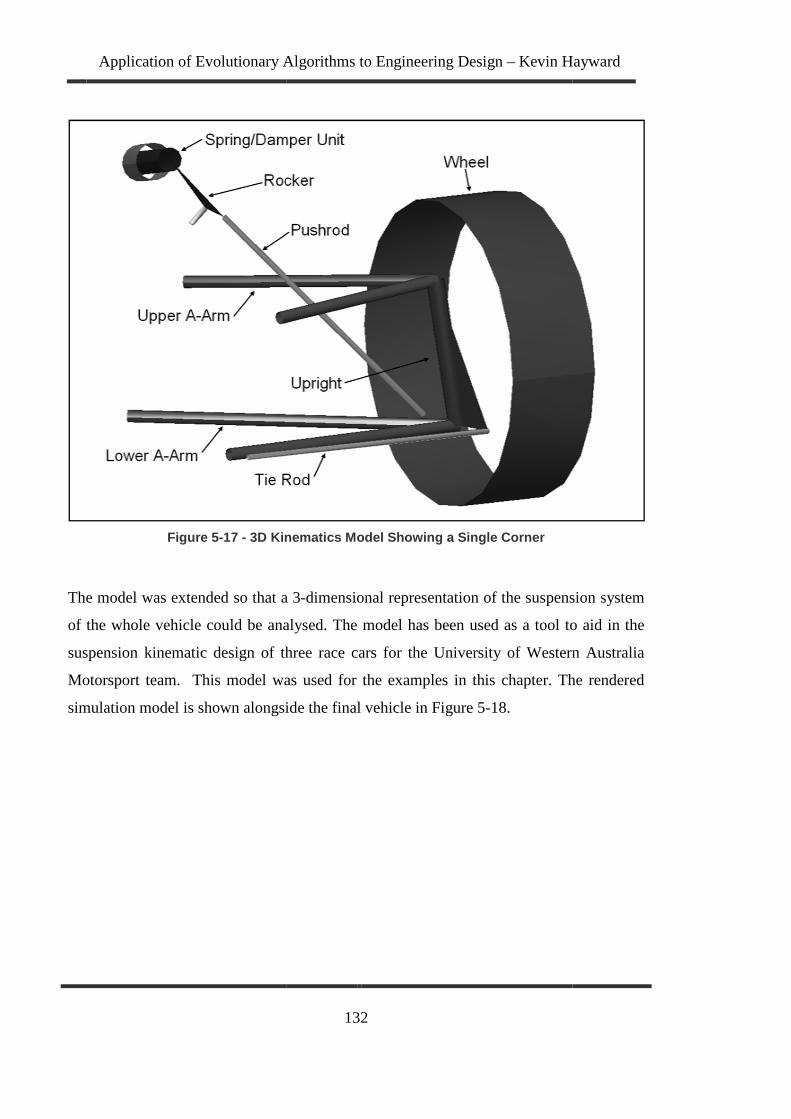
Application of Evolutionary Algorithms to Engineering Design
Figure 5-17 - 3D Kinematics Model Showing a Single Corner
The model was extended so that a 3
of the whole vehicle could be analysed. The model has been used as a tool to aid in the
suspension kinematic design of three race cars for the University of Western Australia
Motorsport team. This model was used for the example
simulation model is shown alongside the final vehicle in
Application of Evolutionary Algorithms to Engineering Design – Kevin Hayward
132
3D Kinematics Model Showing a Single Corner
that a 3-dimensional representation of the suspension system
of the whole vehicle could be analysed. The model has been used as a tool to aid in the
suspension kinematic design of three race cars for the University of Western Australia
This model was used for the examples in this chapter. The rendered
simulation model is shown alongside the final vehicle in Figure 5-18.
Kevin Hayward
on of the suspension system
of the whole vehicle could be analysed. The model has been used as a tool to aid in the
suspension kinematic design of three race cars for the University of Western Australia
s in this chapter. The rendered

Application of Evolutionary Algorithms to Engineering Design
Figure 5- 18
5.2.2 Different Repre
Bäck et al. (1997) make the following comment
solve problems:
Expert knowledge about the problem needs to be incorporated into the
representation and the operators in order to guide the search process and
increase convergence velocity
In order to demonstrate this, a simple problem was set up showing two different
representations of the variables involved.
One of the important issues of suspension design is the camber of the wheel throughout
its travel. A simple objective was defined
25mm of vertical wheel
difference between the camber gain and the desired camber gain.
Application of Evolutionary Algorithms to Engineering Design
133
18 - 2004 UWAM Racing Car (Vehicle & Kinematic Model)
Different Representations
make the following comment about using evolutionary algorithms to
Expert knowledge about the problem needs to be incorporated into the
representation and the operators in order to guide the search process and
increase convergence velocity.
In order to demonstrate this, a simple problem was set up showing two different
representations of the variables involved.
One of the important issues of suspension design is the camber of the wheel throughout
A simple objective was defined so that camber would increase 1 degree for
of vertical wheel movement. The error function was defined as the absolute
difference between the camber gain and the desired camber gain.
Application of Evolutionary Algorithms to Engineering Design – Kevin Hayward
2004 UWAM Racing Car (Vehicle & Kinematic Model)
about using evolutionary algorithms to
Expert knowledge about the problem needs to be incorporated into the
representation and the operators in order to guide the search process and
In order to demonstrate this, a simple problem was set up showing two different
One of the important issues of suspension design is the camber of the wheel throughout
that camber would increase 1 degree for
movement. The error function was defined as the absolute

Application of Evolutionary Algorithms to Engineering Design
Figure 5-19 - Camber Gain with Suspension Travel
Figure 5-19 is a depiction of the camber gain due to suspension travel. Camber is defined
as the angle between the vertical and the wheel angle. Negative camber is when
the wheel is tilted towards the inside. Typically a double A
increase the negative camber with upwards movement of the wheel.
The representation for the A-arms
dimensional problem. Geometry of the spring and rocker system had no bearing on the
camber, so was ignored. These simplifications created a problem that had 4 points in 2
dimensional space to be determined. The 8 variables in this problem were represented in
two different ways. One method was defining each of the x and y co
points as a variable. This is shown graphically
Application of Evolutionary Algorithms to Engineering Design – Kevin Hayward
134
Camber Gain with Suspension Travel
is a depiction of the camber gain due to suspension travel. Camber is defined
as the angle between the vertical and the wheel angle. Negative camber is when
the wheel is tilted towards the inside. Typically a double A-arm suspension system will
increase the negative camber with upwards movement of the wheel.
arms was set so that it could be considered a two
problem. Geometry of the spring and rocker system had no bearing on the
so was ignored. These simplifications created a problem that had 4 points in 2
dimensional space to be determined. The 8 variables in this problem were represented in
ferent ways. One method was defining each of the x and y co-ordinates of the 4
points as a variable. This is shown graphically in Figure 5-20.
Kevin Hayward
is a depiction of the camber gain due to suspension travel. Camber is defined
as the angle between the vertical and the wheel angle. Negative camber is when the top of
arm suspension system will
was set so that it could be considered a two-
problem. Geometry of the spring and rocker system had no bearing on the
so was ignored. These simplifications created a problem that had 4 points in 2-
dimensional space to be determined. The 8 variables in this problem were represented in
ordinates of the 4

Application of Evolutionary Algorithms to Engineering Design – Kevin Hayward
135
Figure 5-20 - x-y Representation
The second method introduced different variables to define the points involved. The 8
variables used to determine the points consisted of:
• The swing arm length (SAL)
• The roll centre (RC)
• x co-ordinate for point 2
• y co-ordinate for point 2
• The upright height
• The king-pin inclination
• x co-ordinate for point 1
• The length of the upper arm as a percentage of the lower arm
This representation introduces accepted vehicle suspension parameters. This is shown
graphically in Figure 5-21.

Application of Evolutionary Algorithms to Engineering Design – Kevin Hayward
136
Figure 5-21 - SAL Representation
The second representation (SAL) shows the application of problem specific knowledge.
While both representations fully define the mechanism, the second representation presents
variables as they would be treated by a designer. For example, the location of the
instantaneous centre gives a large indication of how a four-bar linkage will move, because
it is an approximation of the point about which the tyre will rotate. Including the swing-
arm length and the roll centre height as variables allows for the instantaneous centre to be
defined by two variables instead of the eight required in the x-y representation.
Both representations were used with the same error function defined above. The
evolutionary algorithm developed in Chapter 4 was applied to both, 50 times. The results
are given below.

Application of Evolutionary Algorithms to Engineering Design – Kevin Hayward
137
Table 5-4 - Comparison between Representations
SAL Representati on
Mean 3.54E-08
Std. Dev. 1.08E-07
x-y Representation
Mean 1.10E-06
Std. Dev. 3.65E-06
t-value -2.06
The results clearly showed improvement when the problem was set up with variables
designed with problem-specific knowledge. The average error for the two different
representations plotted against the number of generations is shown below.
Figure 5-22 - Average Error vs. Generations (For 2 Different Parameter Representations)
This shows the improved convergence velocity for the SAL representation over the x-y
representation, hence the inclusion of problem specific knowledge in the representation of
the variables improves the performance of the evolutionary optimisation.
Average Error vs. Generations
-8
-7
-6
-5
-4
-3
-2
-1
00 10 20 30 40 50 60
Generation
Log(
Err
or)
SAL Representation xy Respresentation

Application of Evolutionary Algorithms to Engineering Design
5.2.3 Determining Parameter Relati
Recording the process of the evolutionary algorithm produces useful information
addition to a final problem solution. In the previous example we can look at the variation
of the different variables over time. The graph below
performance of all the points covered by a single run for the variable defining the swing
arm length. An optimum swing arm length of around 1500 was seen. Furthermore a clear
and expected relationship can be seen between the
Figure 5-23 - Performance vs. Swing Arm Length
The other variables did not appear to have a similar relationship. For example
variable that is common to both of the representations
Figure 5-24 shows the performance of each point plotted against this variable.
Application of Evolutionary Algorithms to Engineering Design – Kevin Hayward
138
Determining Parameter Relationships
Recording the process of the evolutionary algorithm produces useful information
addition to a final problem solution. In the previous example we can look at the variation
of the different variables over time. The graph below (Figure 5-23)
performance of all the points covered by a single run for the variable defining the swing
An optimum swing arm length of around 1500 was seen. Furthermore a clear
relationship can be seen between the camber gain and the swing arm length.
Performance vs. Swing Arm Length
not appear to have a similar relationship. For example
h of the representations is the x co-ordinate for point 1.
shows the performance of each point plotted against this variable.
Kevin Hayward
Recording the process of the evolutionary algorithm produces useful information, in
addition to a final problem solution. In the previous example we can look at the variation
) shows the
performance of all the points covered by a single run for the variable defining the swing
An optimum swing arm length of around 1500 was seen. Furthermore a clear
camber gain and the swing arm length.
not appear to have a similar relationship. For example, one such
ordinate for point 1.

Application of Evolutionary Algorithms to Engineering Design
The log of the error was plotted to clearly show where the best performing solutions
existed. In this case the best solutions were found when the x
its maximum. However it appears from this that there is no strong relationship between
performance and this variable
only one optimal solution is computed. In order to support such relationships it is useful
to perform more than one run with the algorithm. The previous two graphs are r
below with five different runs shown on the same graph.
Application of Evolutionary Algorithms to Engineering Design
139
Figure 5-24 - Performance vs. x1
f the error was plotted to clearly show where the best performing solutions
In this case the best solutions were found when the x-coordinate of point 1 was at
However it appears from this that there is no strong relationship between
this variable. It should be noted that only running the algorithm
only one optimal solution is computed. In order to support such relationships it is useful
to perform more than one run with the algorithm. The previous two graphs are r
below with five different runs shown on the same graph.
Application of Evolutionary Algorithms to Engineering Design – Kevin Hayward
f the error was plotted to clearly show where the best performing solutions
coordinate of point 1 was at
However it appears from this that there is no strong relationship between
running the algorithm once,
only one optimal solution is computed. In order to support such relationships it is useful
to perform more than one run with the algorithm. The previous two graphs are reproduced

Application of Evolutionary Algorithms to Engineering Design
Figure 5-25 - Performance vs. Swing Arm Length (5 Runs Overlaid)
Application of Evolutionary Algorithms to Engineering Design – Kevin Hayward
140
Performance vs. Swing Arm Length (5 Runs Overlaid)
Kevin Hayward

Application of Evolutionary Algorithms to Engineering Design
Figure
By conducting multiple runs of the algorithm there is further confirmation that there is a
strong relationship between performance and SAL
was close to 1500, and the shape of the relationsh
is further evidence that no
co-ordinate of point 1.
variables produced similar results t
relationships between performance and any one of the variables when the problem was
solved in its x-y co-ordinate representation.
This is a very simple analysis of the variables and will only really
there is a distinct relationship between one of the variables and performance. However,
should such a relationship be found, it can become very useful in determining the
behaviour of the system for different conditions. For example
above it was hypothesized that there was a strong relationship between the swing arm
Application of Evolutionary Algorithms to Engineering Design
141
Figure 5-26 - Performanc e vs. x1 (5 Runs Overlaid)
By conducting multiple runs of the algorithm there is further confirmation that there is a
strong relationship between performance and SAL. In each run the final value of the SAL
was close to 1500, and the shape of the relationship appears consistent. Furthermore
is further evidence that no unique relationship exists between the performance and the x
ordinate of point 1. Different optimum values were found for each of the 5 runs.
variables produced similar results to the x coordinate of point 1. There were n
between performance and any one of the variables when the problem was
ordinate representation.
This is a very simple analysis of the variables and will only really
there is a distinct relationship between one of the variables and performance. However,
should such a relationship be found, it can become very useful in determining the
behaviour of the system for different conditions. For example, f
above it was hypothesized that there was a strong relationship between the swing arm
Application of Evolutionary Algorithms to Engineering Design – Kevin Hayward
e vs. x1 (5 Runs Overlaid)
By conducting multiple runs of the algorithm there is further confirmation that there is a
. In each run the final value of the SAL
ip appears consistent. Furthermore there
relationship exists between the performance and the x
Different optimum values were found for each of the 5 runs. Other
There were no noticeable
between performance and any one of the variables when the problem was
This is a very simple analysis of the variables and will only really aid the designer when
there is a distinct relationship between one of the variables and performance. However,
should such a relationship be found, it can become very useful in determining the
from the results shown
above it was hypothesized that there was a strong relationship between the swing arm

Application of Evolutionary Algorithms to Engineering Design
length and the camber properties of the system. A further hypothesis was made that a
relationship could be formed linking the different swing arm len
amounts of camber gain. To test these, the evolutionary algorithm was used to find
solutions for a variety of camber gains ranging from 0.2 to 2 degrees for 25mm of vertical
suspension travel. The graph below shows the average SAL of 5
the camber gains.
Figure 5-27 - Swing Arm Length vs. Camber Gain
A clear relationship was seen linking the Swing Arm Length and the amount of camber
gain. The graph also showed that for low camber gains
arm length was not satisfactory to continue the relationship.
Given knowledge of the problem this relationship was not surprising. The swing arm
length determines how far the instantaneous centre
Application of Evolutionary Algorithms to Engineering Design – Kevin Hayward
142
length and the camber properties of the system. A further hypothesis was made that a
relationship could be formed linking the different swing arm lengths with different
amounts of camber gain. To test these, the evolutionary algorithm was used to find
solutions for a variety of camber gains ranging from 0.2 to 2 degrees for 25mm of vertical
suspension travel. The graph below shows the average SAL of 5 different runs for each of
Swing Arm Length vs. Camber Gain
A clear relationship was seen linking the Swing Arm Length and the amount of camber
hat for low camber gains, the available range for the swing
arm length was not satisfactory to continue the relationship.
Given knowledge of the problem this relationship was not surprising. The swing arm
length determines how far the instantaneous centre of the suspension system is away from
Kevin Hayward
length and the camber properties of the system. A further hypothesis was made that a
gths with different
amounts of camber gain. To test these, the evolutionary algorithm was used to find
solutions for a variety of camber gains ranging from 0.2 to 2 degrees for 25mm of vertical
different runs for each of
A clear relationship was seen linking the Swing Arm Length and the amount of camber
the available range for the swing
Given knowledge of the problem this relationship was not surprising. The swing arm
of the suspension system is away from

Application of Evolutionary Algorithms to Engineering Design
the wheel. If we model the wheel as being attached to a beam connected to this point we
get the following geometric relationship for the camber gain (for 25mm travel) of the
wheel:
Plotted this against the previous graphs yielded the following:
Figure
The values determined through the theoretical model matched tho
algorithm quite well. Longer swing arm lengths seem to give slightly higher camber gains
than expected by the theoretical model. This is likely to be the result of the length
difference between the upper and lower arms.
Application of Evolutionary Algorithms to Engineering Design
143
the wheel. If we model the wheel as being attached to a beam connected to this point we
get the following geometric relationship for the camber gain (for 25mm travel) of the
Equation 5-15
Plotted this against the previous graphs yielded the following:
Figure 5-28 - Swing Arm Length vs. Camber Gain
The values determined through the theoretical model matched tho
algorithm quite well. Longer swing arm lengths seem to give slightly higher camber gains
than expected by the theoretical model. This is likely to be the result of the length
difference between the upper and lower arms. This showed that the algorithm may be
)sin(
25
CamberGainSAL=
Application of Evolutionary Algorithms to Engineering Design – Kevin Hayward
the wheel. If we model the wheel as being attached to a beam connected to this point we
get the following geometric relationship for the camber gain (for 25mm travel) of the
Swing Arm Length vs. Camber Gain
The values determined through the theoretical model matched those of the evolutionary
algorithm quite well. Longer swing arm lengths seem to give slightly higher camber gains
than expected by the theoretical model. This is likely to be the result of the length
hat the algorithm may be

Application of Evolutionary Algorithms to Engineering Design – Kevin Hayward
144
used as a tool to test theoretical models as well as pointing towards relationships that may
not be known by the user.
5.2.4 Multiple Objectives
Continuing to use the kinematic design of suspension in this example causes a number of
issues to be raised. The algorithm has been shown to be effective at determining solutions
for different camber gain values, and useful to test hypotheses concerning problem
variables. However, as with many engineering design problems, this example cannot
easily be formed to provide an appropriate single objective function. In this case the
camber gain for the suspension is not the only objective that will determine performance:
there are a number of properties of a suspension system that may determine the overall
performance of the vehicle. Some examples include:
• Roll centre movement as a result of suspension movement
• Toe change versus vertical travel
• Track change due to suspension movement
• Caster change due to suspension movement
• Ackermann effects in steering geometry
It is difficult to form these issues into a single objective suitable for the evolutionary
algorithms. There are a number of methods for dealing with multiple objectives, which
are considered beyond the scope of this work. (Section 3.7)
If strong relationships between some variables can be found (as shown in the previous
section) some simple methods of dealing with multiple objectives can be found. To
demonstrate this, the previous example was extended. In addition to desiring a camber
gain of 1 degree for 25mm of travel, another objective was added requiring a
minimization of roll centre movement for a given roll angle. In order to simulate what
would occur during a roll movement, two sides of the suspension were required. The

Application of Evolutionary Algorithms to Engineering Design
vehicle was assumed to be symmetrical and the roll was defined by one side having a
vertical movement of 25mm while the other had a vertical movement of
error function was defined as the absolute difference between the original roll
height and the roll centre height after the roll motion.
algorithm yielded the following result.
The initial roll centre height was
relationship to performance. These are shown below for 5 overlaid runs.
6 This is a simplification as roll will exhibit uneven vertical movements for the right and left wheels;
however it was considered a reasonable approximation for non
close to the ground.
Application of Evolutionary Algorithms to Engineering Design
145
vehicle was assumed to be symmetrical and the roll was defined by one side having a
vertical movement of 25mm while the other had a vertical movement of
error function was defined as the absolute difference between the original roll
height and the roll centre height after the roll motion. Applying the evolutionary
algorithm yielded the following result.
Figure 5-29 - Performance vs. Generations
The initial roll centre height was the only variable that appeared to have a significant
relationship to performance. These are shown below for 5 overlaid runs.
This is a simplification as roll will exhibit uneven vertical movements for the right and left wheels;
however it was considered a reasonable approximation for non-compliant suspensions with roll centres
Application of Evolutionary Algorithms to Engineering Design – Kevin Hayward
vehicle was assumed to be symmetrical and the roll was defined by one side having a
vertical movement of 25mm while the other had a vertical movement of -25mm.6 The
error function was defined as the absolute difference between the original roll centre
Applying the evolutionary
the only variable that appeared to have a significant
relationship to performance. These are shown below for 5 overlaid runs.
This is a simplification as roll will exhibit uneven vertical movements for the right and left wheels;
compliant suspensions with roll centres

Application of Evolutionary Algorithms to Engineering Design
Figure 5- 30
The roll centre height is usually decided independent
on the lateral load transfer of the vehicle during cornering.
the roll centre to reduce movement is not a desirable outcome.
function, no consideration was made
these issues, both the swing arm length and the roll centre were set at known values and
the problem repeated with a reduced number of variables. The results are shown below
when the SAL was set to 1540mm (according to the relationship found in
and the roll centre to an arbitrary height of 25mm.
Application of Evolutionary Algorithms to Engineering Design – Kevin Hayward
146
30 - Performance vs. Roll Centre
ecided independently of the geometry, as it has an effect
on the lateral load transfer of the vehicle during cornering. Hence defining the position of
the roll centre to reduce movement is not a desirable outcome. Using this simple objective
onsideration was made of the camber properties. In order to account for
both the swing arm length and the roll centre were set at known values and
the problem repeated with a reduced number of variables. The results are shown below
AL was set to 1540mm (according to the relationship found in section
and the roll centre to an arbitrary height of 25mm.
Kevin Hayward
as it has an effect
Hence defining the position of
Using this simple objective
. In order to account for
both the swing arm length and the roll centre were set at known values and
the problem repeated with a reduced number of variables. The results are shown below
section 5.2.3)

Application of Evolutionary Algorithms to Engineering Design – Kevin Hayward
147
Figure 5-31 - Performance vs. Generations (Paramete rs Unrestricted vs. Restricted)
This showed that by restricting the changes in the number of variables that can be altered,
the amount of roll centre movement was increased. However it should be noted that the
camber gain was close to what was originally desired. For example the candidate for the
last run had a camber gain of 0.9981 degrees per 25mm vertical wheel travel. This was
within 0.2% of the desired camber gain value and would be insignificant in vehicle
construction. In addition to finding a valid solution, there was some indication that there
may be a relationship between the relative lengths of the upper and lower arms and the
overall performance. The graph below shows this.

Application of Evolutionary Algorithms to Engineering Design
Figure 5-32 - Perfo rmance vs. Ratio of Upper and Lower Arm Lengths
A final test involved fixing all the variables apart from this single variable to ascertain
whether it may be used as an independent variable to affect the roll centre movement. The
SAL and the RC were set as above. All other variables were set arbitrarily in the middle
of their available range. The following
Application of Evolutionary Algorithms to Engineering Design – Kevin Hayward
148
rmance vs. Ratio of Upper and Lower Arm Lengths
all the variables apart from this single variable to ascertain
whether it may be used as an independent variable to affect the roll centre movement. The
above. All other variables were set arbitrarily in the middle
of their available range. The following relationship was found.
Kevin Hayward
rmance vs. Ratio of Upper and Lower Arm Lengths
all the variables apart from this single variable to ascertain
whether it may be used as an independent variable to affect the roll centre movement. The
above. All other variables were set arbitrarily in the middle

Application of Evolutionary Algorithms to Engineering Design
Figure 5- 33
This example shows a clear relationship. However
quite a lot more effort. Given these results, it is probable that while the other variables
have an effect on the roll centre movement
arm may be altered to find a reasonable solution that minimises roll centre movement.
Using this approach has revealed a significant amount of information
It also highlights the difficulties that additional objective functions introduce
Familiarity with the problem can help to determine some of these relationships with the
aid of the information gathered by the evolutionary process. While it is clear that
relationships were easy to determine by looking at the performance against indivi
variables, it takes some knowledge to be able to determine which relationships can be
acted upon. The example in this section is the relationship between the roll centre height
and the roll centre movement. The inexperienced designer m
Application of Evolutionary Algorithms to Engineering Design
149
33 - Performance vs. Ratio of Upper and Lower Arm Length s
e shows a clear relationship. However, finding this relationship involved
quite a lot more effort. Given these results, it is probable that while the other variables
ffect on the roll centre movement, they can be fixed and the length of the upper
arm may be altered to find a reasonable solution that minimises roll centre movement.
Using this approach has revealed a significant amount of information
It also highlights the difficulties that additional objective functions introduce
Familiarity with the problem can help to determine some of these relationships with the
aid of the information gathered by the evolutionary process. While it is clear that
relationships were easy to determine by looking at the performance against indivi
it takes some knowledge to be able to determine which relationships can be
acted upon. The example in this section is the relationship between the roll centre height
and the roll centre movement. The inexperienced designer might set the rol
Application of Evolutionary Algorithms to Engineering Design – Kevin Hayward
Performance vs. Ratio of Upper and Lower Arm Length s
finding this relationship involved
quite a lot more effort. Given these results, it is probable that while the other variables
and the length of the upper
arm may be altered to find a reasonable solution that minimises roll centre movement.
Using this approach has revealed a significant amount of information about the problem.
It also highlights the difficulties that additional objective functions introduce.
Familiarity with the problem can help to determine some of these relationships with the
aid of the information gathered by the evolutionary process. While it is clear that
relationships were easy to determine by looking at the performance against individual
it takes some knowledge to be able to determine which relationships can be
acted upon. The example in this section is the relationship between the roll centre height
set the roll centre height

Application of Evolutionary Algorithms to Engineering Design – Kevin Hayward
150
in a location to deliver minimum movement. While being correct for one particular
objective, it would cause problems with other objectives.
5.2.5 Problems with System Level Designing
The suspension kinematic problem is a good example of a real problem faced during
vehicle design. As mentioned in the previous section, there are a number of criteria that
define a successful suspension system. This immediately leads to multiple objectives. For
a racing car the case can be made that a more appropriate single objective problem exists
that involves the kinematic objectives outlined in this section.
Typically, goal of designing a racing car is to achieve the minimum lap time, for a given
number of laps (Section 2.5). When designing a suspension system, a number of
assumptions are made to determine what suspension properties will lead to a vehicle with
a minimum lap time. Often these assumptions are based on empirical evidence and
include some amount of subjectivity. In this chapter both a camber gain and a roll-centre
movement objective were analysed. In both cases an arbitrary ideal was decided. Ideally
the suspension problem could be included as part of an optimisation run that includes the
whole vehicle. That way the designer is freed from having to define multiple objectives
and their ideal values. This is also the case with many of the other design areas involved
with the design of a racing car (Section 2.7).

Application of Evolutionary Algorithms to Engineering Design – Kevin Hayward
151
6 Evolving Racing Cars
In Chapter 5, evolutionary algorithms were applied to problems to show the potential
performance of the technique, how key variables in a problem can be identified, issues
with variable representation, and some of the limitations of using the algorithms. In this
section the evolutionary algorithms are applied to optimise parameters that can effectively
define a whole vehicle. This shows the application of the algorithms in the early stages of
the design process: concept evaluation; and preliminary design.
The lap-time simulation (10 Appendix A: Lap Time Simulation) was designed to be a
computationally quick approximation, so does not offer the accuracy required to make
detailed design decisions. However, the following section will show that application of
evolutionary algorithms yield valuable information as to the direction to take in vehicle
design, as well as giving an idea of how sensitive the performance of a vehicle would be
to various parameters.
This section applies an evolutionary algorithm to the problem of designing a Formula
SAE vehicle. The author has been involved in the formula SAE competition for 5 years
with the University of Western Australia (UWA) Motorsport team. During that time
UWA vehicles have won design awards 3 times in international competitions. This should
allow adequate comparison to be made between the results of the optimisation and a
world-class vehicle. The Formula SAE competition provides a good case study for the
following reasons:
• The rules are not very restrictive and allow for a range of conceptual differences
between cars;
• Vehicles must undergo a number of different vehicle tests that can be simulated
readily, and require different vehicle configurations for success;
• A commonly accepted “best” solution to the rules is unlikely to exist, because of
the youth of the competition and the complexity created by conflicting
requirements of the different tests, as well as it being a non-professional
competition.

Application of Evolutionary Algorithms to Engineering Design – Kevin Hayward
152
6.1 The Formula SAE Competition
The Formula SAE (FSAE) rules start with the following statement of purpose:
The Formula SAE ® Series competitions challenge teams of university
undergraduate and graduate students to conceive, design, fabricate and compete
with small, formula style, autocross racing cars. To give teams the maximum design
flexibility and the freedom to express their creativity and imaginations there are
very few restrictions on the overall vehicle design. Teams typically spend eight to
twelve months designing, building, testing and preparing their vehicles before a
competition. [Formula SAE Rules 2007, Section1.1]
Thus the competition focuses on design flexibility, for non-professional teams, in short
time frames. During the competition the teams put their vehicles through a series of
dynamic tests. These are:
• Skidpan – Vehicles are timed over a constant radius circle in both the clockwise
and anti-clockwise direction.
• Acceleration – Vehicles are timed from a standing start along a 75m straight.
• Autocross – Vehicles are timed from a standing start over a short autocross track
which includes a range of features such as chicanes, straights, and curves as
defined in the rules.
• Endurance – Vehicles are timed over 22km (14 miles) of a track similar to an
autocross track. In addition, the fuel usage of each vehicle is measured to calculate
a fuel economy score.
For a vehicle to be successful in the competition it is necessary to perform credibly in all
the dynamic events. However, given the difference between events it is also clear that
different parameters of the vehicle will have different effects on the performance of the
vehicle. For example brakes are likely to be important for the autocross and endurance,
but are unlikely to be required at all in the acceleration and the skidpan events.

Application of Evolutionary Algorithms to Engineering Design – Kevin Hayward
153
In order to investigate the design parameters of a vehicle, the evolutionary process was
applied to the parameters for each of these events individually. This showed that the ideal
parameters for each individual event are different. In addition, the parameters for the
vehicle were tuned for all the events according to the cumulative scores given in the rules
(SAE 2007):
Dynamic Events
Skid-Pad 50
Acceleration 75
Autocross 150
Fuel Economy 50
Endurance 350
Total Points 675
The points for each individual competition are evaluated by the following formulas:
Equation 6-1
Equation 6-2
Equation 6-3
Equation 6-4
5.21)/184.6(
1)/184.6(5.47
2min
2
+−−
=T
TSkidpan your
5.31)/8.5(
1)/8.5(5.71
min
+−−
=T
TonAccelerati your
5.71)/(
1)/(5.142
minmax
max +−−
=TT
TTAutocross your
1)/(
1)/(50
minmax
max
−−
=VV
VVEconomy your

Application of Evolutionary Algorithms to Engineering Design – Kevin Hayward
154
Equation 6-5
6.2 Experiment Setup
The vehicle was assumed to be symmetric with the same tire model for all four tyres, and
the evolutionary algorithms were programmed to alter the following vehicle variables:
• Mass
• Centre of Gravity Height
• Weight Distribution (Front-to-Rear)
• Front-to-Rear Spring Stiffness Distribution (% Front)
• Front & Rear Spring Progression
• Front & Rear Anti-Roll Bar Stiffness
• Front & Rear Anti-Roll Bar Progression
• Front & Rear Roll-Centre Heights
• Differential Torque Bias Ratio
• Brake Balance (Front-to-Rear)
• Front Sprocket Teeth
• Rear Sprocket Teeth
• Front and Rear Initial Cambers
• Front and Rear Camber Coefficients
• Caster Angle (Front)
• Engine Power (Multiplier)
• Upper Gear Change RPM
• Lower Gear Change RPM
• Frontal Area
• Coefficient of Drag
• Coefficient of Lift (-ve)
• Centre of Pressure Height
• Centre of Pressure (Front-to-Rear)
501)/(
1)/(300
minmax
max +−−
=TT
TTEndurance your

Application of Evolutionary Algorithms to Engineering Design – Kevin Hayward
155
This is a total of 29 parameters, and while it in no way represents all possible vehicle
parameters, it makes for a sizeable problem. It is customary for designers to aim for the
extreme limits of some of these variables. For example, designers generally aim to have a
vehicle that is as light as possible, with the lowest drag coefficient, and the highest engine
power. These design goals are clearly demonstrated in the results. However they are
included in the optimisation for two reasons: firstly an idea of the sensitivity of the
vehicle performance can be found; and secondly it is possible that there will be cases
where the designer is mistaken in these assumptions.
Following this study, another optimisation was run using similar parameters with a few
conceptual packages in which the designer has a clear choice between substantially
different options
• Option 1 – A different engine package is used that uses half of the fuel, produces
half of the power, but weighs 40kg less
• Option 2 – The designer is able to choose between using an aerodynamic package
or not. Choosing wings means the vehicle is able to produce 40kg downforce at
60kph, with a fixed weight penalty of 40kg. The winged vehicle also has an
increase in drag, and a raised centre of pressure height.
• Option 3 – A different set of tyres are used that have a higher peak grip, but are
more sensitive to camber angles.
These conceptual differences are very close to some of the variety in existing Formula
SAE vehicles. The numbers were based on anecdotal evidence. In the simulation, each of
these options was defined as either on or off.
The track for the autocross and endurance events was determined using onboard data
acquisition equipment on the University of Western Australia’s 2004 Formula SAE
vehicle. The data was collected during a test session prior to the 2005 United States
competition. The same data was used for both events. However in order to simulate the

Application of Evolutionary Algorithms to Engineering Design
higher speeds seen in the endurance event
curvature of the track for that event.
6.3 Non-Conceptual Optimisation Results
The following section summarises the results for optimisation
options (smaller engine, aerodynamic package, different tyres)
provided in Appendix B: Chapter 7
Figure
Figure 6-1 shows the best skidpan times for each of five optimisation runs. The average
of the five runs was 5.053s as shown by the dashed line, the best time was 5.041s, and the
range between best and worst runs was 0.028s (0.55%).
Application of Evolutionary Algorithms to Engineering Design – Kevin Hayward
156
endurance event, a scaling factor was applied to decre
curvature of the track for that event.
Conceptual Optimisation Results
The following section summarises the results for optimisation without the conceptual
options (smaller engine, aerodynamic package, different tyres). Tabulated results are
Chapter 7 Non-Conceptual Results.
Figure 6-1 - Skidpan Times
shows the best skidpan times for each of five optimisation runs. The average
s was 5.053s as shown by the dashed line, the best time was 5.041s, and the
range between best and worst runs was 0.028s (0.55%).
Kevin Hayward
a scaling factor was applied to decrease the
without the conceptual
Tabulated results are
shows the best skidpan times for each of five optimisation runs. The average
s was 5.053s as shown by the dashed line, the best time was 5.041s, and the

Application of Evolutionary Algorithms to Engineering Design
Figure 6-2 shows the best acceleration times for each of five optimisation runs. The
average of the five runs was 4.339s as shown by the dashed line, the best time was
4.333s, and the range between best and worst runs was 0.014s (0.32%).
Figure 6-3 shows the best autocross times for each of five optimisation runs. The average
of the five runs was 21.388s as shown by the dashed line, the best time was 21.371s, and
the range between best and worst runs was 0.048s (0.22%).
Application of Evolutionary Algorithms to Engineering Design
157
Figure 6-2 - Acceleration Times
he best acceleration times for each of five optimisation runs. The
average of the five runs was 4.339s as shown by the dashed line, the best time was
4.333s, and the range between best and worst runs was 0.014s (0.32%).
Figure 6-3 - Autocross Times
shows the best autocross times for each of five optimisation runs. The average
of the five runs was 21.388s as shown by the dashed line, the best time was 21.371s, and
e between best and worst runs was 0.048s (0.22%).
Application of Evolutionary Algorithms to Engineering Design – Kevin Hayward
he best acceleration times for each of five optimisation runs. The
average of the five runs was 4.339s as shown by the dashed line, the best time was
4.333s, and the range between best and worst runs was 0.014s (0.32%).
shows the best autocross times for each of five optimisation runs. The average
of the five runs was 21.388s as shown by the dashed line, the best time was 21.371s, and

Application of Evolutionary Algorithms to Engineering Design
Figure
Figure 6-4 shows the best endurance times for each of five optimisation runs. The ave
of the five runs was 18.556s as shown by the dashed line, the best time
the range between best and worst runs was 0.0
the time per lap.
In order to calculate the overall score
the minimum times for skidpan, acceleration, autocross, and endurance were taken as the
minimums found in the optimisations given above. This results in the following table:
EventSkidpanAcceAutocrossEndurance
Table
Fuel economy score was taken as the maximum 50 points.
Application of Evolutionary Algorithms to Engineering Design – Kevin Hayward
158
Figure 6-4 - Endurance Times
shows the best endurance times for each of five optimisation runs. The ave
s as shown by the dashed line, the best time was 18.534
the range between best and worst runs was 0.054s (0.29%). The times shown represent
In order to calculate the overall score according to the equations presented in section
the minimum times for skidpan, acceleration, autocross, and endurance were taken as the
minimums found in the optimisations given above. This results in the following table:
Event Time (s) Skidpan 5.041 Acceleration 4.333 Autocross 21.371 Endurance 18.534
Table 6-1 - Minimum Times
Fuel economy score was taken as the maximum 50 points.
Kevin Hayward
shows the best endurance times for each of five optimisation runs. The average
was 18.534s, and
The times shown represent
d in section 6.1
the minimum times for skidpan, acceleration, autocross, and endurance were taken as the
minimums found in the optimisations given above. This results in the following table:

Application of Evolutionary Algorithms to Engineering Design
Figure 6-5 shows the best overall score for each of five optimisation runs. The average of
the five runs was 653.5 points as shown by the dashed line, the best score was 657.6
points, and the range between best and worst runs wa
Application of Evolutionary Algorithms to Engineering Design
159
Figure 6-5 – Overall Scores
shows the best overall score for each of five optimisation runs. The average of
the five runs was 653.5 points as shown by the dashed line, the best score was 657.6
points, and the range between best and worst runs was 7.7 point (1.18%).
Application of Evolutionary Algorithms to Engineering Design – Kevin Hayward
shows the best overall score for each of five optimisation runs. The average of
the five runs was 653.5 points as shown by the dashed line, the best score was 657.6
s 7.7 point (1.18%).
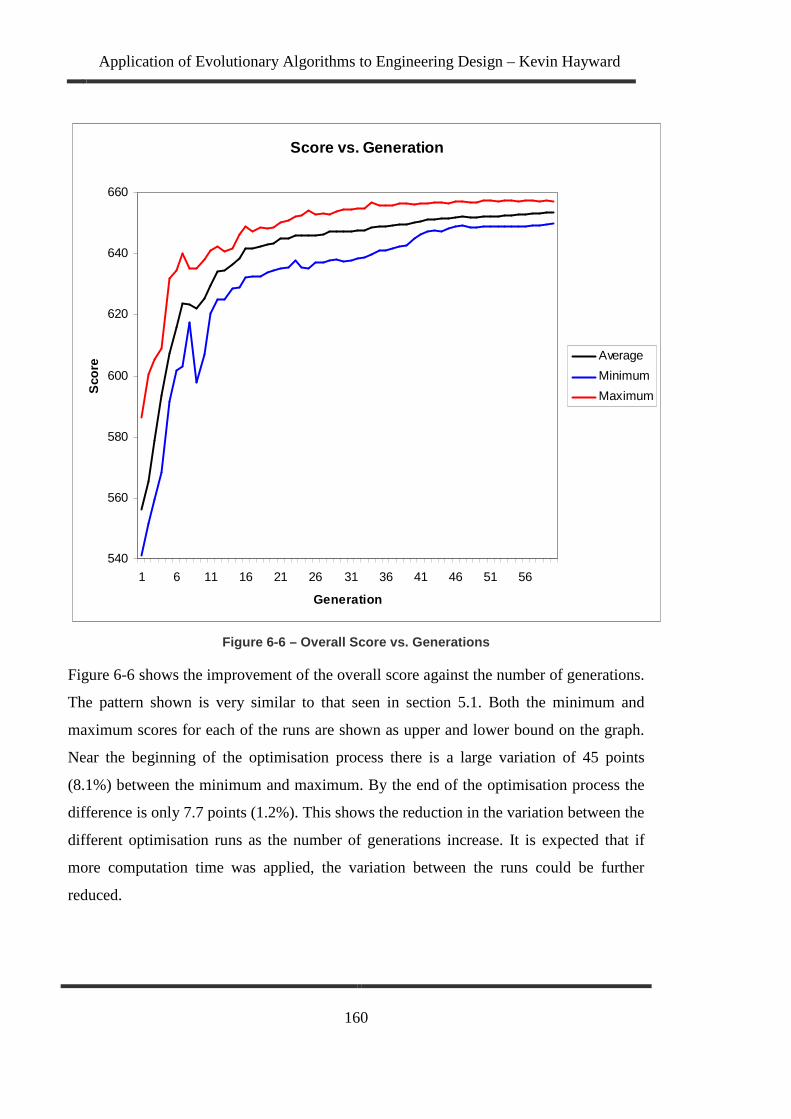
Application of Evolutionary Algorithms to Engineering Design – Kevin Hayward
160
Figure 6-6 – Overall Score vs. Generations
Figure 6-6 shows the improvement of the overall score against the number of generations.
The pattern shown is very similar to that seen in section 5.1. Both the minimum and
maximum scores for each of the runs are shown as upper and lower bound on the graph.
Near the beginning of the optimisation process there is a large variation of 45 points
(8.1%) between the minimum and maximum. By the end of the optimisation process the
difference is only 7.7 points (1.2%). This shows the reduction in the variation between the
different optimisation runs as the number of generations increase. It is expected that if
more computation time was applied, the variation between the runs could be further
reduced.
Score vs. Generation
540
560
580
600
620
640
660
1 6 11 16 21 26 31 36 41 46 51 56
Generation
Sco
re
Average
Minimum
Maximum

Application of Evolutionary Algorithms to Engineering Design – Kevin Hayward
161
Run Skidpan Acceleration Autocross Endurance Fuel Total 1 44.9 62.8 147.6 344.6 50.0 649.9 2 44.4 67.2 149.5 346.6 50.0 657.6 3 45.2 63.8 147.5 343.4 50.0 649.9 4 44.9 65.1 148.1 347.8 50.0 656.0 5 43.7 70.6 146.7 342.9 50.0 653.9
Average 44.6 65.9 147.9 345.0 50.0 653.5 Range 1.5 7.9 2.8 5.0 0.0 7.7
Table 6-2 - Overall Score for Individual Runs
Table 6-2 shows the individual scores that made up the best candidate found in each of
the five runs. The best score for each event is highlighted. It is interesting to note that in
no individual run was the best score found for every event.
6.3.1 Discussion
The results show that each event requires different parameter values for an optimum
solution. Each of the events represents a real world racing challenge. The acceleration
event mimics a drag race, the skidpan is a real world test and could be compared to oval
track racing, while the autocross and endurance mimic track racing. However the results
from the overall optimisation will likely yield the best design directions for the vehicles.
The following table shows the simulated overall scores for the best of each optimisation.
Car Optimised for:
Skidpan (/ 50)
Acceleration (/75)
Autocross (/150)
Endurance (/350)
Fuel (/50)
Total (/675)
Skidpan 50 35 113 287 50 535 Acceleration 0 75 38 159 50 322 Autocross 44 58 150 349 50 651 Endurance 43 59 149 350 50 652 Overall Score 44 67 149 347 50 658
Table 6-3 - Overall Scores for Different Vehicles
Each of the optimised cars scored highest for its respective event. Cars optimised for the
Autocross and the Endurance event also perform very well overall. This was not
unexpected, as a car designed to compete well on a typical race track must have the
ability to both accelerate and corner well. However, a car tuned solely to corner well
does not need to brake or accelerate well, and a car tuned solely for acceleration does not
need to brake or corner well. An extreme example of this is a Drag Racing car, which
corners very poorly.

Application of Evolutionary Algorithms to Engineering Design – Kevin Hayward
162
Some of the parameters required to tune for a particular event are fixed in the
manufacture of a car. An example in Formula SAE is the Centre of Gravity Fore-Aft
location. A table below shows the centre of gravity positions for the best vehicle in each
event.
Car Optimised for: Rear Weight % Skidpan 0.51 Acceleration 0.65 Autocross 0.60 Endurance 0.62 Overall 0.61
Table 6-4 - Ideal Rear Weight Bias
This shows that a car that corners well has close to equal weight front-to-rear, whereas a
car that accelerates well has a high rear weight bias, and a good track car lies somewhere
between these two.
Some other vehicle parameters are made to be adjustable. Results from the optimisation
of all the events can lead to an idea of how much adjustment is needed. For example we
can look at the initial rear camber.
Car Optimised for:
Rear Initial Camber
Skidpan -1.30 Acceleration 0.00 Autocross -0.76 Endurance -0.68 Overall -0.90
Table 6-5 - Ideal Rear Camber
In this case if the vehicle was constructed with rear camber tuneable between 0 and -1.3
degrees then the car can be set up optimally for each of the events. However care should
be taken not to treat variables independently. In this example, the rear camber angle of a
vehicle is also affected by the camber compensation, a parameter that is generally not
tuneable. In this example the ideal acceleration vehicle had no camber compensation,
while the other events required significant camber compensation. In this case, one

Application of Evolutionary Algorithms to Engineering Design
possible solution would be to increase the available tuning range
determined during later design stages.
As shown in Section 5.2.3
to overall performance
vehicle. For each of the optimisation runs minimum vehicle mass was ideal. This
relationship can clearly be seen by plotting all of the solutions as shown below.
It should be noted at this point that the mass was taken as the sum of the vehicle and
driver mass. A minimum vehicle mass of 220kg was taken, which represented the
approximate full fuel mass of the 2004 UWA FSAE vehicle
suit and helmet) was taken as 85kg.
7 Other FSAE cars are lighter than the 220kg of the 2004 UWA FSAE entry, including later entries from the
same team. However this number was used as minimising the mass was a primary design goal of the team
Application of Evolutionary Algorithms to Engineering Design
163
solution would be to increase the available tuning range
determined during later design stages.
5.2.3, relationships that directly link the value of certain parameters
all performance may be found. One example in this test was the overall mass of the
vehicle. For each of the optimisation runs minimum vehicle mass was ideal. This
relationship can clearly be seen by plotting all of the solutions as shown below.
Figure 6-7 - Performance vs. Mass
It should be noted at this point that the mass was taken as the sum of the vehicle and
driver mass. A minimum vehicle mass of 220kg was taken, which represented the
uel mass of the 2004 UWA FSAE vehicle7. A driver mass (including
suit and helmet) was taken as 85kg.
Other FSAE cars are lighter than the 220kg of the 2004 UWA FSAE entry, including later entries from the
same team. However this number was used as minimising the mass was a primary design goal of the team
Application of Evolutionary Algorithms to Engineering Design – Kevin Hayward
solution would be to increase the available tuning range; this would be
directly link the value of certain parameters
. One example in this test was the overall mass of the
vehicle. For each of the optimisation runs minimum vehicle mass was ideal. This
relationship can clearly be seen by plotting all of the solutions as shown below.
It should be noted at this point that the mass was taken as the sum of the vehicle and
driver mass. A minimum vehicle mass of 220kg was taken, which represented the
. A driver mass (including
Other FSAE cars are lighter than the 220kg of the 2004 UWA FSAE entry, including later entries from the
same team. However this number was used as minimising the mass was a primary design goal of the team

Application of Evolutionary Algorithms to Engineering Design – Kevin Hayward
164
This graph is from optimising the overall competition. In order to show it is a
minimisation problem the score found was subtracted from the maximum possible score.
This is represented on the Y axis with the title of Available Points. The line represents
the lower boundary of the set of points. This relationship is clearly one-way and would
indicate that further reductions in vehicle mass will likely yield higher performance.
Other parameters show relationships that are not as direct. The following example shows
the performance relationship for the Final Drive Ratio8.
and it represented the lowest mass achievable by the team at the time. The maximum mass is close to the
value of the 2001 UWA FSAE entry. As such; this mass range spans from the first to the last UWA FSAE
vehicle that the author was actively involved in designing. 8 The final drive ratio is calculated by dividing the number of rear sprocket teeth by the number of front
sprocket teeth.

Application of Evolutionary Algorithms to Engineering Design
These relationships not only show an ideal value but they give an idea of the sensitivity of
the result. For example
3. In addition, it shows that
it. Two dimensional plots can be made for each of the parameters against performance. It
is then very easy to visually assess whether a clear relationship can be found.
These graphs can also
environments. For this example we can look at the Torque Bias Ratio (TBR) of the
differential. For the autocross event
the Skidpan event the lowest TBR v
In a very simple analysis one could conclude that lower TBR values are better for
skidpan, and the higher better for autocross. For example
of these two values (~3.5)
design decision could easily be disproved by looking at the following graphs.
Application of Evolutionary Algorithms to Engineering Design
165
Figure 6-8 - Performance vs. Final Dr ive Ratio
These relationships not only show an ideal value but they give an idea of the sensitivity of
the result. For example, the Final Drive Ratio in Figure 6-8 gives an ideal value
it shows that decreasing the drive ratio is more detrimental than
Two dimensional plots can be made for each of the parameters against performance. It
very easy to visually assess whether a clear relationship can be found.
These graphs can also help to determine how variables are linked to particular
environments. For this example we can look at the Torque Bias Ratio (TBR) of the
differential. For the autocross event, a reasonably high TBR of around 6 was optimal. For
the Skidpan event the lowest TBR value of 1 (representing an open differential) was ideal.
In a very simple analysis one could conclude that lower TBR values are better for
skidpan, and the higher better for autocross. For example, designing a TBR in the middle
of these two values (~3.5) might end up working reasonably in both environments. Such a
design decision could easily be disproved by looking at the following graphs.
Application of Evolutionary Algorithms to Engineering Design – Kevin Hayward
ive Ratio
These relationships not only show an ideal value but they give an idea of the sensitivity of
gives an ideal value of about
more detrimental than increasing
Two dimensional plots can be made for each of the parameters against performance. It
very easy to visually assess whether a clear relationship can be found.
how variables are linked to particular
environments. For this example we can look at the Torque Bias Ratio (TBR) of the
a reasonably high TBR of around 6 was optimal. For
alue of 1 (representing an open differential) was ideal.
In a very simple analysis one could conclude that lower TBR values are better for
designing a TBR in the middle
might end up working reasonably in both environments. Such a
design decision could easily be disproved by looking at the following graphs.

Application of Evolutionary Algorithms to Engineering Design
Figure 6-9 -
Figure 6- 10
Application of Evolutionary Algorithms to Engineering Design – Kevin Hayward
166
- Torque Bias Ratio for Autocross
10 - Torque Bias Ratio for Skidpan
Kevin Hayward

Application of Evolutionary Algorithms to Engineering Design – Kevin Hayward
167
What is clear in these graphs is that for the autocross event the time gets worse either side
of the ideal value of around 6. However for there to be any real improvement in skidpan
performance the TBR would have to be less than 2. Hence the original suggestion that
some value in-between 1 and 6 would be ideal seems highly unlikely. Further evidence
for this is that the ideal TBR value for the overall competition was found to be close to 6.
Care must be taken not to dismiss variables that do not show clear relationships to
performance. In the example of the lap time simulation (10 Appendix A: Lap Time
Simulation), an important calculation in each step of the simulation required the
computation of the roll moment distribution. This value determines how lateral load
transfer is distributed between the front and rear axles, in turn having a noticeable effect
on vehicle performance. In the optimisation run there are 9 different variables that affect
this calculation:
• Spring Stiffness Distribution (% Front)
• Front & Rear Spring Progression
• Front & Rear Anti-Roll Bar Stiffness
• Front & Rear Anti-Roll Bar Progression
• Front & Rear Roll-Centre Heights
Dependent variables like these are unlikely to show a clear relationship between
performance and their given value, but performance may still be very sensitive to changes
in any one of these variables because of their influence on roll moment distribution.
6.4 Conceptual Optimisation Results
The following section summarises the results for optimisation where the three conceptual
options (smaller engine, aerodynamic package, different tyres) were included. This was
achieved by adding a continuous variable with values between 0 and 1 for each of the
options. If the given value was less than 0.5 then the option was not used, if it was greater
than 0.5 it was. This creates a discrete on/off variable for the optimisation routine.
Tabulated results are provided in Appendix C: Chapter 7 Conceptual Results.

Application of Evolutionary Algorithms to Engineering Design
Figure
Figure 6-11 shows the best skidpan times for each of five
of the five runs was 5.066s as shown by the dashed line, the best time was 5.0
range between best and worst runs was 0.0
Figure
Figure 6-12 shows the best acceleration times for each of five optimisation runs. The
average of the five runs was 4.3
4.337s, and the range between best and worst runs was 0.01
Application of Evolutionary Algorithms to Engineering Design – Kevin Hayward
168
Figure 6-11 - Skidpan Times
shows the best skidpan times for each of five optimisation runs. The average
s as shown by the dashed line, the best time was 5.055
range between best and worst runs was 0.043s (0.85%).
Figure 6-12 - Acceleration Times
shows the best acceleration times for each of five optimisation runs. The
average of the five runs was 4.345s as shown by the dashed line, the best time was
s, and the range between best and worst runs was 0.014s (0.32%).
Kevin Hayward
optimisation runs. The average
55s, and the
shows the best acceleration times for each of five optimisation runs. The
s as shown by the dashed line, the best time was

Application of Evolutionary Algorithms to Engineering Design
Figure 6-13 shows the best autocross times for each of five optimisation runs. The
average of the five runs was 21.
21.79s, and the range between best and worst runs was 0.
Figure 6-14 shows the best endurance times for each o
average of the five runs was 18.
18.95s, and the range between best and worst runs was 0.
Application of Evolutionary Algorithms to Engineering Design
169
Figure 6-13 - Autocross Times
shows the best autocross times for each of five optimisation runs. The
average of the five runs was 21.88s as shown by the dashed line, the best time was
s, and the range between best and worst runs was 0.33s (1.51
Figure 6-14 - Endurance Times
shows the best endurance times for each of five optimisation runs. The
average of the five runs was 18.99s as shown by the dashed line, the best time was
s, and the range between best and worst runs was 0.1s (0.53%).
Application of Evolutionary Algorithms to Engineering Design – Kevin Hayward
shows the best autocross times for each of five optimisation runs. The
hed line, the best time was
1.51%).
f five optimisation runs. The
s as shown by the dashed line, the best time was
%).

Application of Evolutionary Algorithms to Engineering Design
In order to calculate the overall score according to the equations present
the minimum times for skidpan, acceleration, autocross, and endurance were taken as the
minimums found in the optimisations given above. This results in the following table:
EventSkidpanAccAutocrossEndurance
Table
Fuel economy was taken as 50 points where the smaller engine was used, and 25 points
where the larger engine was used.
Figure
Figure 6-15 shows the best overall score for each of five optimisation runs. The average
of the five runs was 613.7 points as shown by the dashed line,
points, and the range between best and worst runs was
Application of Evolutionary Algorithms to Engineering Design – Kevin Hayward
170
In order to calculate the overall score according to the equations presented in section
the minimum times for skidpan, acceleration, autocross, and endurance were taken as the
minimums found in the optimisations given above. This results in the following table:
Event Time (s) Skidpan 5.055 Acceleration 4.337 Autocross 21.790 Endurance 18.950
Table 6-6 - Minimum Times
Fuel economy was taken as 50 points where the smaller engine was used, and 25 points
Figure 6-15 – Overall Scores
shows the best overall score for each of five optimisation runs. The average
points as shown by the dashed line, the best score was 621.1
points, and the range between best and worst runs was 29.6 points (4.82%).
Kevin Hayward
ed in section 6.1
the minimum times for skidpan, acceleration, autocross, and endurance were taken as the
minimums found in the optimisations given above. This results in the following table:
Fuel economy was taken as 50 points where the smaller engine was used, and 25 points
shows the best overall score for each of five optimisation runs. The average
core was 621.1

Application of Evolutionary Algorithms to Engineering Design – Kevin Hayward
171
Figure 6-16 – Overall Score vs. Generations (Concep tual Optimisation)
Figure 6-16 shows the improvement of the overall score against the number of
generations. The pattern shown is very similar to that seen in section 5.1 and for the non-
conceptual optimisation. Both the minimum and maximum scores for each of the runs are
shown as the upper and lower bounds on the graph. Near the beginning of the
optimisation process there is a large variation of 37.5 points (7.2%) between the
minimum and maximum. By the end of the optimisation process the difference is still
quite high at 29.6 points (4.8%). It is expected that if more computation time was applied,
the variation between the runs could be further reduced.
Score vs. Generation
490
510
530
550
570
590
610
630
1 6 11 16 21 26 31 36 41 46 51 56
Generation
Sco
re
Average
Minimum
Maximum

Application of Evolutionary Algorithms to Engineering Design – Kevin Hayward
172
Run Skidpan Acceleration Autocross Endurance Fuel Total 1 42.2 57.7 148.5 345.8 50.0 619.2 2 41.1 57.2 147.3 345.8 50.0 616.4 3 42.8 58.0 148.1 346.3 50.0 620.2 4 38.0 67.3 138.3 323.0 50.0 591.5 5 41.8 58.2 148.4 347.8 50.0 621.1
Average 41.2 59.7 146.1 341.7 50.0 613.7 Range 4.8 10.1 10.2 24.8 0.0 29.6
Table 6-7 - Overall Score for Individual Runs
Table 6-7 shows the individual scores that made up the best candidate found in each of
the five runs. The best score for each event is highlighted. As with the non-conceptual
optimisation, no individual run gave the best score found for every event.
6.4.1 Discussion
The first note of interest is the increased range between optimisation runs for each event.
This is most notably observed for the overall competition score. For the non-conceptual
optimisation the final range between the best and worst runs was 7.7 points. In the
conceptual optimisation the range was 29.6 points. This was caused by one of the five
runs in the conceptual analysis having a different conceptual choice. This shows the
sensitivity of the concepts which is discussed in section 6.6.
The following table analyses how a vehicle optimised for each event would perform
overall.
Car Optimised for:
Skidpan (/50)
Acceleration (/75)
Autocross (/150)
Endurance (/350)
Fuel (/50)
Total (/675)
Skidpan 50 0 87 253 50 441 Acceleration 18 75 66 204 25 388 Autocross 42 51 150 349 25 617 Endurance 42 53 149 350 25 619 Overall 42 58 148 348 25 621
Table 6-8 - Overall Scores for Different Vehicles ( Conceptual Optimisation)
The results end up similar to those seen in the previous section. Each optimised car
performs optimally in its respective event.

Application of Evolutionary Algorithms to Engineering Design
With the different conceptual options
performance have been altered. The best example of these is the mass of the vehicle. This
relationship is shown below.
Table 6
Two of the options involved changing the mass of the vehicle. This in turn has affected
the graph. The ideal mass is now no longer the minimum mass. This is an important
design discovery because
Application of Evolutionary Algorithms to Engineering Design
173
With the different conceptual options, some of the relationships betwe
performance have been altered. The best example of these is the mass of the vehicle. This
relationship is shown below.
6-9 - Performance vs. Mass (Conceptual Optimisation)
options involved changing the mass of the vehicle. This in turn has affected
the graph. The ideal mass is now no longer the minimum mass. This is an important
because performance may not always increase as mass is decreased
Application of Evolutionary Algorithms to Engineering Design – Kevin Hayward
some of the relationships between variables and
performance have been altered. The best example of these is the mass of the vehicle. This
Performance vs. Mass (Conceptual Optimisation)
options involved changing the mass of the vehicle. This in turn has affected
the graph. The ideal mass is now no longer the minimum mass. This is an important
as mass is decreased.

Application of Evolutionary Algorithms to Engineering Design – Kevin Hayward
174
At this stage a design decision for the different options is much more informed and is
summarised below:
Option 1: Different Engine
The lower mass of the engine was certainly advantageous for skidpan, however the lack
of power meant that each other event required the original heavier, and more powerful
engine to increase performance. This option would not be used because overall
performance would be reduced.
Option 2: Addition of an Aerodynamic Package
The higher mass due to the aerodynamic package meant that it would not feature on a car
designed for acceleration. However for all other events the higher mass was more than
compensated for by the increase in grip due to down-force. This option should be used.
Option 3: Different Tyre
The tyre with higher grip, but increased camber sensitivity appeared to be the better of the
two tyres for all of the events. This option would be used.
Each of these options was similar to design decisions made within the University of
Western Australia Formula SAE team. In these particular cases the different engine was
not chosen, which appeared to be the right choice. Wings were not added to the car,
which appeared to be the wrong choice. A tyre with lower camber sensitivity was chosen,
however this decision was made on the basis of tyre wear encountered during testing, a
variable not included in the simulation. It would appear from these results that the team
should investigate the addition of wings to future vehicles as an avenue to increase
performance.

Application of Evolutionary Algorithms to Engineering Design – Kevin Hayward
175
6.5 Comparison to Existing Vehicles
There is value in comparing the results of the simulation to the specifications of an
existing vehicle. The vehicle used for comparison will be the 2004 University of Western
Australia (UWA) Formula SAE vehicle. The vehicle was quite successful, winning the
Design Award (for the best designed vehicle) and coming 2nd overall in the 2005 United
States Formula SAE Competition. (This was the largest competition of the year with 140
teams.) The vehicle was the fourth (and last) UWA vehicle in which the author was
involved in the design process. During that time the on-track performance of each
successive vehicle improved.
The following graph shows the comparison of the autocross simulation and the original
data.
Table 6-10 - Simulated vs. Actual Vehicle Velocity
Vehicle Velocity
0
5
10
15
20
25
Vel
ocity
(m
/s)
Actual (22.68s) Simulated (22.30s)

Application of Evolutionary Algorithms to Engineering Design – Kevin Hayward
176
The correlation is reasonable, considering the simulation was designed with limited
accuracy to increase computational speed. It is also not surprising that the simulated time
is faster. The author, the driver of the vehicle, has had prior experience in the car and its
predecessors; however he is not a professional driver. This point is highlighted as the
simulation and optimisation process will give an idea of the capabilities of the vehicle, the
actual final performance is likely to be different. The simulation always runs at the limit
of the vehicle performance envelope, while the driver is not able to do that.
A similar graph can be used to compare the simulations of the existing vehicle and one
that has been optimised using the evolutionary algorithms.
Table 6-11 - Optimised vs. UWA Vehicle (Autocross)
The optimised vehicle shows a simulated improvement of 0.61s (3%). The following
table shows the difference in competition scores between the optimised car and the UWA
vehicle.
Vehicle Velocity
0
5
10
15
20
25
Vel
ocity
(m
/s)
Optimised (21.69s) UWA Vehicle (22.30s)

Application of Evolutionary Algorithms to Engineering Design – Kevin Hayward
177
Car Skidpan
(/50) Acceleration
(/75) Autocross
(/150) Endurance
(/350) Fuel (/50)
Total (/675)
UWA Vehicle 33 60 134 306 25 559 Optimised 42 58 148 348 25 621
Table 6-12 - Optimised vs. UWA Vehicle (Overall Sco re)
The difference in scores of 62 points is very significant. Notably, the optimised vehicle
outperformed the UWA Vehicle in all but one event. This is significant for two reasons:
first it offers an idea of how to make changes in the design of the car to improve
performance; secondly it shows that the evolutionary optimisation process was able to
provide a solution that was superior to 4 years of design processes that did not use these
methods.
6.6 Parameter Sensitivity
Throughout this and previous sections, there has been some mention of determining the
sensitivity of the final result to various parameters. This is invaluable in the design
process as it provides knowledge to the designer about the required manufacturing
tolerances, as well as suggesting tuning ranges for particular parameters. Furthermore as
the design process continues, opportunities may arise to alter the boundaries of some of
the tuned parameters. For example if engine power was shown to be very important to the
final result, the design team might investigate forced induction systems.
In the previous sections there were examples of plotting parameter values for all of the
tested solutions against their relative performance. This has been shown to provide insight
into various relationships. Other methods include finding the range and/or standard
deviation for a particular variable over a number of evolutionary runs. For example we
can look at the Brake Bias Parameter for the non-conceptual optimisation of the vehicle.
The values, range and standard deviation are given below.

Application of Evolutionary Algorithms to Engineering Design – Kevin Hayward
178
Run Brake
Balance 1 1.18 2 0.93 3 1.18 4 1.02 5 0.96
Average 1.05 Range 0.26
Std. Dev. 0.10
Table 6-13 - Brake Balance for 5 Runs
Clearly there is not much variation between each of the runs. This indicates that the ideal
brake balance is likely to be within the range provided. Secondly, the standard deviation
would indicate that approximately 95% of the brake balance solutions would fall between
±2 standard deviations of the mean. This would give 95% of the values between 0.85 and
1.25. This gives an idea of the tuneable range for this parameter. Such information could
be useful immediately for the starting parameters for the detailed design of an appropriate
pedal box and brake bias adjustment device. This is supported by the previous method of
plotting the performance against the parameter values as shown below (Figure 6-17).

Application of Evolutionary Algorithms to Engineering Design
This process can be repeated for any of the relevant variables.
varying each parameter of the final solution
performance of the vehicle. This is a procedure shown
parameters of the best solution of the conceptual optimisation were altered to test
sensitivity. The table below shows the
This gives an idea of wh
greatest margin. However, caution must be
parameters have been optimised to suit the original conceptual choice. In reality
performance decreases
Application of Evolutionary Algorithms to Engineering Design
179
Figure 6-17 - Ideal Brake Bias Range
This process can be repeated for any of the relevant variables. Another approach
each parameter of the final solution to determine its relative effect on the
performance of the vehicle. This is a procedure shown by Crolla et al. (2002).
parameters of the best solution of the conceptual optimisation were altered to test
. The table below shows the effects of deciding on different concepts
Configuration Score Difference Original 621 0 Different Engine 535 -86 Remove Wings 586 -35 Different Tyre 615 -6
Table 6-14 - Conceptual Sensitivity
This gives an idea of which of the conceptual options affects the performance by
margin. However, caution must be exercised because
parameters have been optimised to suit the original conceptual choice. In reality
performance decreases caused by changing concepts is likely to be smaller than indicated.
Application of Evolutionary Algorithms to Engineering Design – Kevin Hayward
Another approach involves
ts relative effect on the
by Crolla et al. (2002). To test this,
parameters of the best solution of the conceptual optimisation were altered to test
different concepts.
ich of the conceptual options affects the performance by the
exercised because the rest of the vehicle
parameters have been optimised to suit the original conceptual choice. In reality, the
by changing concepts is likely to be smaller than indicated.

Application of Evolutionary Algorithms to Engineering Design – Kevin Hayward
180
This method should mainly be used as a post optimisation check rather than a decision
making process. The process can be used on other parameters as well. A few examples
are given below.
Configuration Score Difference Original 621 0 Mass (+5%) 602 -19 Mass (-5%) 641 20 Engine Power (+5%) 629 8 Engine Power (-5%) 612 -9 Weight Dist. (+5% Rearwards) 616 -5 Weight Dist. (-5% Rearwards) 619 -2 Final Drive (+5%) 619 -2 Final Drive (-5%) 621 0 Caster (+5%) 621 0 Caster (-5%) 621 0
Table 6-15 - Selected Parameter Sensitivity
This analysis could be carried out with all parameters, and if percentages of change are
small enough, some linear optimisation of the final solution can be found. This method
can also be used as a way to rank the effect of individual parameters on the final solution.
For further detail on this method see Crolla et al. (2000).
6.7 Conclusion
This chapter has shown how evolutionary algorithms can be effectively used in the design
process for a difficult problem. Good results were found within short time frames. The
final result of the optimisation showed a simulated improvement of close to 10% over an
already existing and successful UWA vehicle. The process highlighted some conceptual
changes that could be made to future vehicles to improve performance. The optimisation
process was also time-effective, as a single run of the algorithm for the full competition
took approximately 1.5 hours of computation time on the author’s desktop computer, well
within the specifications for the algorithm outlined in Chapter 4. The algorithm was also
able to find good solutions for the different environments of the different competition
events. This would indicate that if conditions were to change, the process could be
repeated quickly with good results.

Application of Evolutionary Algorithms to Engineering Design – Kevin Hayward
181
Using the evolutionary process also has the advantage of providing a large amount of data
from throughout the search process. If this data is recorded, simple data mining and
visualization techniques can be used to determine the relationship of parameters to the
overall performance of the problem.
There were a number of different types of parameters used in the same optimisation
routine without problems. There were Boolean variables such as the choice of concepts,
discrete variables such as sprocket sizes, and continuous variables such as spring
stiffness. There were parameters that appeared to have a direct link to performance, as
well as parameters that interacted with each other to affect performance. Despite this
variation the algorithm gave good robust results.
The evolutionary algorithm approach appears to be very effective during the conceptual
design phase. In this particular case, many of the parameters in the design process are set
very early on, but have a large effect on overall performance. A clear example would be
the choice of engines. The evolutionary algorithms could be used to make quick and
accurate decisions during the early stages of design.

Application of Evolutionary Algorithms to Engineering Design – Kevin Hayward
182
7 Conclusion
Evolutionary algorithms are a convenient and robust method to automate the search for
appropriate design solutions to increase the efficiency of the mechanical design process.
A study of current design processes indicated that the evolutionary algorithm’s main use
would be in some automation of the decision making process. The following
requirements of an evolutionary algorithm used to increase design efficiency were
determined:
• Easy to apply to the relevant problem
• Quick
• Reliable
• Scalable
• Ability to adapt to a large number of problems
An algorithm was developed that met these requirements, and was successfully applied to
three motorsport design problems. Using the algorithms to test conceptual changes, which
would occur at the very start of the design process, was shown to provide significant
performance increases to the particular problem of racing car design. This would indicate
that the earlier the algorithms are used, the better the final result.
In order to apply the evolutionary algorithm all that was necessary was to replace one line
of code with a call to a predefined performance function. The designer must supply the
performance function, including a relevant representation of the variables. Representation
of the variables being optimised is very important. Poor variable representation reduces
the performance of the optimisation. The goal should be to try, where possible, to achieve
a direct mapping between performance and the variable. Representation of a design as a
number of relevant variables, and a method to assess its performance are both required in
the product development method, so is quite separate from the application of the
evolutionary algorithms. Once this has been created, the application of the evolutionary
algorithm is quite simple.

Application of Evolutionary Algorithms to Engineering Design – Kevin Hayward
183
Time required to perform the optimisation process was reduced by tuning the algorithm to
give decent results for a relatively small number of iterations. Significant increases in the
convergence speed of the algorithm were found first by using tuning parameters of
different values than those traditionally prescribed. In addition, evolutionary parameters
involved with the control of mutation strength, and distribution were added and made
self-adaptive. These showed significant improvements over traditional algorithms for the
limited number of iterations available.
The algorithm was tuned to be reliable using a mix of uni-modal and multi-modal test
functions. In addition the trade-off between assigning computation to increase
performance or reliability was studied. The more computation time applied to a single
optimisation run, improves the performance, however computation should be split
between multiple runs to improve the reliability of the result.
Scalability of the algorithm was a natural extension of the traditional evolutionary
algorithms. Any number of variables can be used, as the most important tuning
parameters are defined as functions of the number of variables. Testing showed good
results for the algorithm with between 5 and 30 variables without changing any of the
tuning parameters. It is expected that further testing could be conducted and that good
results would be found for an even larger number of variables.
The same evolutionary code was used without modification for each of the three different
motorsport problems, as well as the suite of 13 test functions. This represented a variety
of conditions; large and small problems, uni and multi-modal problems, discrete and
continuous variables, dependent and independent variables, and a range of complexity of
the problems. Focusing on self-adaptive features in the algorithm as well as tuning for a
variety of different test functions, allowed the creation of an algorithm that works
credibly in a number of different situations. By normalising the input variables of the
evolutionary algorithm, a common form was introduced for any variable relevant to the
optimisation. This allowed treatment of any continuous or discrete variable of any
specified range. In each case exactly the same evolutionary code was used, with the

Application of Evolutionary Algorithms to Engineering Design – Kevin Hayward
184
replacement of the relevant performance function. In each case the algorithm gave good
results. It is expected that many more problems could be approached with exactly the
same algorithm.
Of particular interest for the design process was the ability to analyse the data created by
the optimisation process. Relationships of the variables with respect to performance can
be analysed. Much of the data gained is in areas of the search space that offer high
performance potential. This allows the designer to set more suitable ranges of the
variables along with finding clear one-to-one relationships between particular variables
and the performance of the design. This is an area in which much work could still be
done.
Particular note should be made about problems with multiple design objectives, as they
can occur quite frequently in real-world situations. While multi-objectives are
cumbersome to deal with using the simple algorithms presented in this thesis, it is
possible to apply weightings to particular objectives to find a suitable result. The Formula
SAE competition provides one such example. The car must be designed to perform well
in five different events, but its final score is a weighted average of the five events. Also
where possible it may be better to frame the multiple objectives into a larger problem that
has only one objective. In Chapter 5 suspension geometry was discussed with a number
of objectives. In reality this is part of a larger problem of lap-time speed. The same
geometrical problem could be included in a lap time solution which has a single objective.
In conclusion, an evolutionary algorithm was developed with unique mutation control
methods; that was successfully applied to a number of design problems. In each case both
the efficiency of the process and the quality of the final solution were improved.

Application of Evolutionary Algorithms to Engineering Design – Kevin Hayward
185
8 Recommendations for Future Work
There are many avenues where future work may be conducted. This work has focused on
the tuning and application of a particular type of evolutionary algorithm. Other
evolutionary algorithms (or other non-linear multi-modal solvers) could be tested to
provide a comparison between algorithms. However the “No free lunch theorem”
(Wolpert and Macready, 1995) would indicate that on average, algorithms will perform
equally over a complete set of problems. Also given the number of possible approaches to
solving these types of problems it is unlikely that a fair comparison of algorithms could
be achieved.
Of more interest would be the further development of modifications to the algorithm
already presented. During the development of the algorithm it was evident that using
tuning parameters with different values to the accepted norm allowed greater performance
for restricted computational time. In particular, self-adaptation of the mutation parameters
gave a notable increase in performance for the conditions tested. Further work could be
conducted to test these modifications for more problems, and under different amounts of
available computation.
Given that the design process for complex systems can continue over extended periods of
time it may be desirable to implement a continuous evolutionary algorithm. This could
allow the current best results to be displayed at any given time as a design reference point.
Furthermore modifications to the environment or simulation models can be incorporated
as new information about the problem is discovered.
Another area where time might be saved is in the introduction of models with varying
levels of complexity. Early in the evolutionary search process simpler models could be
adopted that provide a rough approximation of the problem, but are quick. As the process
continues the model can be made more accurate as fine-tuning of the solution is needed.

Application of Evolutionary Algorithms to Engineering Design – Kevin Hayward
186
Robustness of the final solutions could be introduced as a part of the performance
evaluations. Non-robust solutions would incur a performance penalty. This could be a
way to introduce the idea of design tolerances into the optimisation. Achieving this will
require some local approximation of the search-space to avoid increasing the computation
time significantly.
During the design process it appears that much use could be made of the analysis of the
data gained throughout the optimisation process. In this thesis there was some coverage of
this by plotting parameters against performance, as well as comparing parameter values
between the results of the same optimisation performed a number of times. More
advanced data-mining techniques could be employed to better determine possible
relationships between parameters and performance. Of particular interest would be in
determining where performance may have a relationship with a number of dependent
variables.
The main recommendation of the author is to continue applying these techniques to new
problems. Through application of the algorithm the true strengths and weaknesses of this
approach will be revealed.

Application of Evolutionary Algorithms to Engineering Design – Kevin Hayward
187
9 Bibliography
Allen, R.W. & Rosenthal, T.J., 1994, Requirements for Vehicle Dynamics Simulation,
Society of Automotive Engineers, Warrendale, PA, USA (Paper No. 940175)
Armstrong-Wilson, C., 2005, Write Line, Racecar Engineering, Vol 15, No. 4, IPC
Media, England, p. 5
Armstrong-Wilson, C., 2002, Write Line, Racecar Engineering, Vol 12, No. 10, IPC
Media, England, p. 5
Bäck, T., Hammel, U. & Schwefel, H.P., 1997, 'Evolutionary Computation: Comments on
the History and Current State', in Evolutionary Computation – The Fossil Record, ed
Fogel, D.B., IEEE Press, New York, USA, pp. 15-28.
Bäck, T. & Schwefel, H.-P., 1996, ‘Evolutionary Computation: An Overview’, in
Proceedings of IEEE International Conference on 20-22 May 1996, pp. 20 – 29
Bäck, T. & Schwefel, H.-P., 1996, ‘An Overview of Evolutionary Algorithms for
Parameter Optimization’, in Evolutionary Computation 1(1), pp. 1 – 23
Bäck, T., 1995, ‘Evolutionary Strategies: An Alternative Evolutionary Algorithm’, in
Artificial Evolution: European Conference, September 4-6, pp. 3-20
Bäck, T., U. & Schwefel, H.P., 1993, ‘An Overview of Evolutionary Algorithms for
Parameter Optimization’, in Evolutionary Computation – The Fossil Record, ed Fogel,
D.B., IEEE Press, New York, USA, pp. 15-28.
Bae, D.S., Lee, J.K., Cho, H.J. & Yae, H., 2000, ‘An Explicit Integration Method for
Realtime Simulation of Multibody Vehicle Models’, in Computer Methods in Applied
Mechanics and Engineering 187 (2000), Elsevier Science S.A., pp 337-350

Application of Evolutionary Algorithms to Engineering Design – Kevin Hayward
188
Baumal A.E., McPhee, J.J. & Calamai, P.H., 1998, ‘Application of Genetic Algorithms to
the Design Optimization of an Active Vehicle Suspension System’, in Computer Methods
in Applied Mechanics and Engineering 163 (1998), Elsevier Science S.A., pp 87-94
Birmingham, R., Cleland, G., Driver, R., and Maffin, D., 1997, Understanding
Engineering Design: Context, Theory and Practice, Prentice Hall, Great Britain.
Booker, J.D., Raines, M. and Swift, K.G., 2001, Designing Capable and Reliable
Products, Butterworth-Heinemann, Oxford.
Cagan, J., Grossmann, I.E. & Hooker, J., 1997, ‘A Connceptual Framework for
Combining Artificial Intelligence and Optimization in Engineering Design’, in Research
in Engineering Design, Springer-Verlag, London, pp 20-34
Candelpergher, A., Gadola, M. & Vetturi, D., 2000, Developments of a Method for Lap
Time Simulation, University of Brescia, Society of Automotive Engineers, Warrendale,
PA, USA (Paper No. 2000-01-3562)
Casanova, D., Sharp, R.S. & Symonds, P., 2001, Construction of Race Circuit Geometry
from On-Car Measurements, Proceedings of the Institute of Mechanical Engineers, Part
D: Jounal of Automobile Engineering, Volume 215, Number 9, pp. 1033-1042
Castellani, F. & Franceschini, G., 2003, The Use of Genetic Algortihms as An Innovative
Tool for Race Car Design, Universtiy of Perugia, Society of Automotive Engineers,
Warrendale, PA, USA (Paper No. 2003-01-1327)
Connair, K.M., Bodie, M.O., Chaumette, P. & Catalan A., 1999, Development of a
Common Vehicle Model for Chassis Control Design, Clemson University, Society of
Automotive Engineers, Warrendale, PA, USA (Paper No. 1999-01-0732)

Application of Evolutionary Algorithms to Engineering Design – Kevin Hayward
189
Costa, L. & Oliveira, P., 2002 ‘An Evolution Strategy for Multiobjective Optimization’ in
Congress on Evolutionary Computation (CEC'2002), Vol. 1, May, pp. 97--102, IEEE
Service Center, Piscataway, New Jersey.
Costin, M. & Phipps, D., 1967, Racing and Sports Car Chassis Design, Bentley
Publishing, UK
Darwin, C., 1985 (Reprint of 1859 Original), The Origin of Species, Penguin Books.
London, UK
Deakin, A. & Crolla, D., 2000, Fundamental Parameter Design Issues Which Determine
Race Car Performance, The University of Leeds, Society of Automotive Engineers,
Warrendale, PA, USA (Paper No. 2000-01-3537)
Deakin, A., Shovlin, A., Brooks, P. & Crolla, D., 1998, ‘Design of a Single Seater Racing
Car Suspension System’, 1998 Motorsports Engineering Conference Proceedings Volume
2: Engines and Drivetrains, Society of Automotive Engineers, Warrendale, PA, USA
(Paper No. 983020)
Dixon, J.C., 1996, Tires, Suspension and Handling, Society of Automotive Engineers,
Warrendale, PA, USA
Dominy, R. & Dominy, J., 1996, ‘The Power of Simulation’, in Racecar Volume 6 No. 2
(Magazine), IPC Media, Croydon, England
Dym, C.L., 1994, Engineering Design, Cambridge University Press, New York.
Ertas, J. & Jones, J.C., 1993, The Engineering Design Process, John Wiley & Sons, New
York

Application of Evolutionary Algorithms to Engineering Design – Kevin Hayward
190
Farshidianfar A. & Ebrahimi, M., 2001, Optimization of Vehicle Driveline Vibrations
Using Genetic Algorithm (GA), University of Bradford, Society of Automotive Engineers,
Warrendale, PA, USA (Paper No. 2001-01-1511)
Fogel, D.B., 1994, 'An Introduction to Simulated Evolutionary Optimization', in
Evolutionary Computation – The Fossil Record, ed Fogel, D.B., IEEE Press, New York,
USA, pp. 3-14.
Fogel, L.J., 1996, ‘Top-Down Evolutionary Engineering’, in Yao, X., Kim, J-H. &
Furuhashi, T. (eds.), 1996, Simulated Evolution and Learning, Springer-Verlag Berlin
Heidelberg, New York, USA, pp. 11-16
Gadola, M., Vetturi D., Cambiaghi D. & Manzo L., 1996, A Tool for Lap Time
Simulation, Society of Automotive Engineers, Warrendale, PA, USA (Paper No. 962529)
Gillespie, T.D., 1992, Fundamentals of Vehicle Dynamics, Society of Automotive
Engineers, Warrendale, PA, USA
Glimmerveen, J.H., 2004, Hands-On Race Car Engineer, Society of Automotive
Engineers, Warrendale, PA, USA
Hacker, K., Lewis, K. & Kasprzak, E.M., 2000, Racecar Optimization and Tradeoff
Analysis in a Parrallel Computing Environment, State University of New York at Buffalo
& Milliken Research Associates Inc., Society of Automotive Engineers, Warrendale, PA,
USA (Paper No. 2000-01-3564)
Haney, P., 2003, The Racing & High-Performance Tire, TV Motorsports, Illinois, USA
Haque, B. and Pawar, K.S., 1998, Development of a Methodology and Tool for Analysing
New Product Design and Development in a Concurrent Engineering Environment (in
Proceedings EDC, 98), Bury St Edmunds: Professional Engineering Publishing, 669-677

Application of Evolutionary Algorithms to Engineering Design – Kevin Hayward
191
He, J. & Yao, x., 2002, ‘From an Individual to a Population: An Analysis of the First
Hitting Time of Population-Based Evolutionary Algorithms’ in IEEE Transactions on
Evolutionary Computation, Vol. 6, No. 5, October, pp. 495-511
Hollins, B. and Pugh, S., 1990, Successful Product Design, Butterworths, London.
Hotten, R., 1998, The Business of Winning, Orion, London. P. xi
Huang, G.Q., 1996, Developing DFX Tools. In: Design for X – Concurrent Engineering
Imperatives, Huang, G.Q. (ed.), Chapman & Hall, London.
Hyeon-Joong Cho; Se-Young Oh; Doo-Hyun Choi, 1998, ‘Fast evolutionary
programming through search momentum and multipleoffspring strategy’ in IEEE World
Congress on Computational Intelligence, 4-9 May, pp. 805 - 809
Hubka, V. and Eder, W.E., 1996, Design Science, Springer-Verlag, Great Britain.
Hutter, M. & Legg, S., 2006, ‘Fitness Uniform Optimization’ in IEEE Transactions on
Evolutionary Computation, Vol. 10, No. 5, October, pp. 568-589
Jin, Y., 2005, ‘Evolutionary Optimization in Uncertain Environments’, in IEEE
Transactions on Evolutionary Computation, Vol. 9, No. 3, June, pp.303-317
Kirkpatrick, S., Gelatt, C.D., & Vecchi M.P., 1983, Optimization by Simulated Annealing,
Science, Vol 220, Number 4598, pp. 671-680.
Lawrence, M., 2002, Colin Chapman: Wayward Genius, Butler & Tanner, England.
Li, K. & Nagai, M., ‘Control and Evaluation of Active Suspension for MDOF Vehicle
Model’, in JSAE Review 20 (1999), Society of Automotive Engineers Japan, pp. 343-348

Application of Evolutionary Algorithms to Engineering Design – Kevin Hayward
192
Liang, Y. & Leung, K-S., 2002, ‘Two-way Mutation Evolution Strategies’ in Proceedings
of the 2002 Congress on Evolutionary Computation, Volume 1, 12-17 May, pp. 789-794
Liu, X. & Yao, X. ‘How to control search step size in fast evolutionary programming’in
Proceedings of the 2002 Congress on Evolutionary Computation (CEC) '02, 12-17 May
2002, pp.652-656, IEEE Press, Piscataway, NJ, USA.
Lowndes, E.M., 1998, Development of an Intermediate DOF Vehicle Dynamics Model for
Optimal Design Studies, Doctor of Philosophy Thesis, Department of Mechanical and
Aerospace Engineering, North Carolina State University
Makita, M., 1999, ‘An Application of Suspension Kinematics for Intermediate Level
Vehicle Handling Simulation’, in JSAE Review 20 (1999), Society of Automotive
Engineers Japan, pp. 471-477
Michalewicz, Z., 1996, ‘Evolutionary Computation: Practical Issues’ in Proceedings of
IEEE International Conference on 20-22 May, pp. 30-39
Milliken, W.F. & Milliken, D.L., 1995, Race Car Vehicle Dynamics, Society of
Automotive Engineers, Warrendale, PA, USA
Mitchell, S.A., Durgavich, J., Damiano, A., Smith, S.J. & MacCraken, R., 2004, Use of
Genetic Algorithms With Multiple Metrics Aimed At the Optimization of Automotive
Suspension Systems, Society of Automotive Engineers, Warrendale, PA, USA (Paper No.
2004-01-3520)
Moline, D., Vaduri, S. & Law, E.H., 2000, Fidelity of Vehicle Models Using Roll Center
Principles, Clemson University, Society of Automotive Engineers, Warrendale, PA, USA
(Paper No. 2000-01-0693)
Mühlmeier, M. & Müller, N., 2002, Optimization of the Driving Line on a Race Track,
Audi Sport, Engineers, Warrendale, PA, USA (Paper No. 2002-01-3339)

Application of Evolutionary Algorithms to Engineering Design – Kevin Hayward
193
Pacejka, H.B., 2005, Tire and Vehicle Dynamics, Society of Automotive Engineers,
Warrendale, PA, USA
Pacejka, H.B. & Bakker, E., 1991, 'The Magic Formula Tyre Model', in Tyre Models For
Vehicle Dynamics, ed Pacejka, H.B., Swets & Zeitlinger, Amsterdam, Netherlands, pp. 1-
18.
Pahl, G. and Beitz, W., 1996, Engineering Design: A Systematic Approach, Springer-
Verlag, London.
Purnell, A.J., 1998, Innovative Computer Technology in Professional Motorsports, Pi
Research Ltd., Society of Automotive Engineers, Warrendale, PA, USA (Paper No.
1999-01-2257)
Pugh, S., 1982, The Design Activity Model, Engineering Design Centre, Loughborough
University of Technology, June.
Pugh, S., 1991, Total Design: Integrated Methods for Successful Product Engineering,
Ramanata, P., 1998, Optimal Vehicle Path Generator Using Optimization Methods,
Masters Thesis, Mechanical Engineering, Virginia Polytechnic Institute and State
University
Roberts, N.W., Winkler, J., Norris, C., Fazio, A. & Van der Schoot, C., 2006, Multi-
Disciplinary Design of the Champ Car Atlantic Race Car, Society of Automotive
Engineers, Warrendale, PA, USA (Paper No. 2006-01-3663)
Roston, G.P. & Sturges, R.H, 1996, ‘Genetic Algorithm Synthesis of Four-Bar
Mechanisms’, in Artificial Intelligence for Engineering Design, Analysis and
Manufacturing, Cambridge University Press, USA, pp. 371-390

Application of Evolutionary Algorithms to Engineering Design – Kevin Hayward
194
Rouelle, C., 2007, 12-Day Racecar Engineering Seminar, Seminar by Claude Roelle,
OptimumG, 6 December, Denver, Colorado
Rubin, Z.J., Munns, S.A. & Moskwa, J.J., 1997, The Development of Vehicular
Powertrain Sytem Modeling Methodologies: Philosophy and Implementation, University
of Wisconsin-Madison, Society of Automotive Engineers, Warrendale, PA, USA (Paper
No. 971089)
Russel, R.S. and Taylor, B.W., 1995, Production and Operations Management: Focusing
on Quality and Competitiveness, Prentice-Hall, New Jersey.
Sayers, M.W., 1996, Vehicle Models for RTS Applications, Mechanical Simulation
Coorporation, Ann Arbor, USA
Sayers, M.W. & Han, D., 1995, ‘A Generic Multibody Vehicle Model for Simulating
Handling and Braking’, Presented at Symposium of the International Association of
Vehicle Dynamics, Ann Arbor, USA
Schwefel, H.-P. (1981). Numerical Optimization of Computer Models. Wiley, Chichester,
England.
Scott Floyd, R. & Harry Law, E., 1994, Simulation and Analysis of Suspension and
Aerodynamic Interactions of Race Cars, Society of Automotive Engineers, Warrendale,
PA, USA (Paper No. 942537)
Sen, P. and Yang, J., 1998, Multiple Criteria Decision Support in Engineering Design,
Springer-Verlag, Great Britain.
Sieglar, B.P., Crolla, D.A. & Deakin, A.J., 2000, Lap Time Simulation: Comparison of
Steady State, Quasi-Static and Transient Racing Car Cornering Strategies, Society of
Automotive Engineers, Warrendale, PA, USA (Paper No. 2000-01-3563)

Application of Evolutionary Algorithms to Engineering Design – Kevin Hayward
195
Smith, C., 1978, Tune To Win, Aero Publishers, Fallbrook, USA
Socha, K. & Kisiel-Dorohinicki, M., 2002, ‘Agent-based evolutionary multiobjective
optimisation’ in The 2002 IEEE world congress on Computational Evolution, May 12–
17, pp. 109-114
Society of Automotive Engineers, 2007, 2007 Formula SAE Rules
Society of Automotive Engineers, 2005, 2005 Formula SAE Rules (With Australian
Amendments)
Staniforth, A., 1999, Competition Car Suspension 3rd Ed., Haynes Publishing, Sparkford,
UK
Starkey, C.V., 1992, Engineering Design Decisions, Edward Arnold, Great Britain.
Sum, R.N., Jr 1992, Activity Management: A Survey and Recommendations for the
DARPA Initiative in Concurrent Engineering, DARPA Technical Paper, 17 January
2001, Tire Databook for Formula SAE Program, Goodyear Technical Center, Akron,
USA
Toussaint, M. & Igel, C., 2002, ‘Neutrality: a necessity for self-adaptation’ in
Proceedings of the 2002 Congress on Evolutionary Computation, Volume 2, pp. 1354 -
1359
Valenzuela, C.L., 2002, ‘A Simple Evolutionary Algorithm for Multi-Objective
Optimization (SEAMO)’ in Congress on Evolutionary Computation (CEC'2002), IEEE
press, Vol. 1, pp. 727-733.
Wagstaff, I., 2005, Buyers Insight: The state of the market in racecar simulation software,
Racecar Engineering, Vol 15, No. 4, IPC Media, England, pp. 69-75

Application of Evolutionary Algorithms to Engineering Design – Kevin Hayward
196
Wolpert, D. and Macready, W., 1995, No Free Lunch Theorems for Search (Technical
Report SFI-TR-95-02-010). Santa Fe Institute
Wright, P., 2003, Ferrari Formula 1: Under the Skin of a Championship Winning F1-
2000, Society of Automotive Engineers, Warrendale, PA, USA (Originally Published by
David Bull Publishing, AZ, USA)
Yao, X., Liu, Y. & Lin, G., 1999, ‘Evolutionary Programming Made Faster’, in IEEE
Transactioons on Evolutionary Computation, Vol. 3, No. 2, July, pp. 82-102
Yao, X. & Liu, Y., 1997, ‘Fast Evolution Strategies’, in Evolutionary Programming VI,
Angeline, P.J., Reynolds, R.G., McDonnell, J.R. & Eberhart, R. (eds.), pp. 151-161
Application of Evolutionary Algorithms to Engineering Design – Kevin Hayward
197
10 Appendix A: Lap Time Simulation
This appendix provides discussion on the lap time simulation created by the author. There
are two primary goals in studying vehicle dynamics. The first is to improve the
performance envelope of a vehicle while the second is to improve the comfort of the
occupants (including driver) of the vehicle. These two goals are often in conflict with
each other and must be balanced for a particular application. In motorsport the overriding
concern is the performance envelope, whiling maintaining the minimum level of driver
comfort to allow effective control of the vehicle. As previously stated in section 2.5, the
primary goal of race car design is the minimisation of the time taken to traverse a given
circuit. Computation methods to determine lap times have been developed over the last 50
years. They have become a useful method of applying the theories of vehicle dynamics to
improve race car performance. Hacker et al. (2000) note that little work has been done,
however, on how to effectively use these simulations in conjunction with advanced
optimisation techniques in a systematic way.
10.1 Simulation Requirements
There are three fundamental requirements for the development of a lap time simulation to
be used effectively with evolutionary algorithms. These are listed below:
• Returns a single value for vehicle performance
• Computationally quick
• Represents the real-world problem with acceptable accuracy
Possibly the most critical requirement of the simulations are that they are computationally
quick. If the simulation is not quick to perform it is difficult to apply an evolutionary
approach as the optimisation technique is highly dependent on the iterative step. The
speed required is linked to the level of accuracy achievable in the simulations. Racing car
simulation is an inherently complex problem. Racing car tyres operate near the limits of
adhesion. This makes the dynamics of race cars extremely non-linear.(Gadola et al. 1996)

Application of Evolutionary Algorithms to Engineering Design – Kevin Hayward
198
However it is important that the simulations exhibit a minimum level of accuracy such
that results do not contradict what would be expected in the physical situation. As
available computation power is increased it is expected that more complex models may be
used to improve the accuracy of the results.
In order to use a simulation program effectively, it is necessary to provide accurate inputs
and validate the results. Purnell (1998) states:
“Accurate simulation demands a great deal of quantitative detail about the
car and this in turn is influencing the direction of the test and measurement
equipment used. Mathematical modelling of the car from simple force
balance models to highly sophisticated lap time simulation or dynamic
response modelling requires accurate data and lots of it. The more realistic
the simulation demanded, the more data is required.”
The simulation model developed must represent the available data. For conceptual
studies simpler models can be used, with the understanding that the results are an
indication of performance, rather than an exact value for what the car can achieve.
The models used in the simulation should reflect this.
10.2 Lap Time Simulation
“… the simulation engineer will demand editing tools to play with the
parameter values to determine their importance to performance, tools to
find optimum values, presentation software and database managers to
handle flow in and out of the simulation software.” (Purnell, 1998)
A Lap time simulator is mainly used during two stages of vehicle development (Crolla &
Deakin, 2000); the design process of a new vehicle, and setup of an existing vehicle.
During the tuning, or setup, of the vehicle, predictions can be made regarding vehicle
adjustments such as changes to aerodynamic trim, springs, dampers, suspension geometry
etc. Using a lap time simulator in this case may reduce the number of iterations that need

Application of Evolutionary Algorithms to Engineering Design – Kevin Hayward
199
to be performed to maximise a race car’s performance for a given track. The second main
use for such a simulator is during the design stage of a vehicle in order to study the effects
of alterations to particular design parameters. It is apparent that assessing small changes
to a pre-existing vehicle would require increased accuracy in both vehicle and circuit
models over simulations used in the early design stages of a vehicle. Siegler et al. (2000)
states:
“... it has a use during the initial design phase after which parameters, such
as the centre of gravity position, cannot be changed. The vehicle can then be
produced so that the fundamental design parameters are close to the
optimum values.”
According to Milliken & Milliken (1995) it is probable that Mercedes Benz were the first
to analytically simulate the performance of a race car around a circuit as early as the late
1930’s. It was clear that by the 1950’s the technique had become more regularly used.
Reference is made to the Cornell Aeronautical Laboratory (CAL) using such analysis to
aid in designing a race circuit at Watkins Glen between 1954 and 1956. Early efforts at
lap time simulation were based on steady state equations calculated by hand. Modern
computing has allowed for increased model complexity and accuracy.
It is difficult to ascertain the current state of the field. Lap time simulators are usually
designed and implemented by individual race teams or companies. Given the competitive
nature of the motorsport industry this information rarely enters the public domain. Deakin
and Crolla (2000) note:
In the 40+ years that the codes have been in use, few papers have been
written which describe how a racing car can be made to go faster and
what design or set-up parameters should be changed to achieve this, such
is the secrecy that enshrouds motor racing.

Application of Evolutionary Algorithms to Engineering Design – Kevin Hayward
200
There are differing levels of model complexity that may be used in lap time simulation. It
is logical that the more complex models require increased computation time. Hence a
trade-off must be made between simulation accuracy and computation time. This
compromise varies for different applications. There are many procedures that can be used
to model a vehicle’s performance over a given circuit. Steady-state, quasi-static and
transient strategies were compared during cornering by Siegler et al. (2000). These three
strategies give an idea of the differing levels of complexity that are used in lap time
simulations. Allen (1994) states that “a model must have sufficient complexity for a given
application but should not be overly complicated”. The reasoning behind minimising
complexity where possible aids in reducing software coding, checking and validation
efforts, also aiding in reducing errors. Candelpergher et al. (2000) also states that one of
the goals of their lap-time simulator was to have a high computation speed to enable the
race engineer to estimate the effect of various setup settings in the shortest possible time.
10.2.1 Program Structure
“When attempting to capture the dynamics of an automobile in a computer-
based simulation, the amount of detail available for inclusion is almost
limitless. In the preliminary design stage, however, most of these details are
of little or no importance. These details, no matter how well researched, can
never completely overcome shortcomings inherent to the basic design.”
(Hacker et al. 2000)
The lap time simulator written for this thesis was designed for parameter studies during
the early stages of racing car design. The complexity of the simulation reflects the need
for fast computation rather than absolute accuracy. A few of the key simulation properties
below:
• Vehicle model is quasi-static
• No driver model is included
• Tracks are assumed to be perfectly flat with uniform grip properties

Application of Evolutionary Algorithms to Engineering Design – Kevin Hayward
201
These have important implications on the results gained from the simulation. Since the
model is quasi-static transient dynamics of the vehicles will be ignored and response to
inputs will be assumed to be instantaneous. This will not allow the program to be used to
study the effects of vehicle response or to enable selection of desirable damper
characteristics. The lack of a driver model assumes that the driver is able to operate the
vehicle at the limit of its performance 100% of the time. This is an unrealistic situation
and does not account for vehicle parameters that may result in a vehicle that is difficult to
control. Likewise assuming track as being perfectly flat with uniform grip is also an
unrealistic situation. However to correct these assumptions would require markedly
increased computation time for the simulation. Were this simulation to be used in a
design cycle it would be likely that once basic vehicle parameters have been decided
more accurate vehicle models could be used in the detail design stages.
Gadola et al. (1996) applies the same assumptions above. Sieglar et al. (2000) also notes
that present simulations (From the year 2000) find the cornering ability of the vehicles
using the quasi-static solution. This allows quick and efficient simulations without
requiring a complicated time-dependent solution. Furthermore, Sieglar et al. show close
correlation between the results of the quasi-static approach and a much more complex
transient model. They do note the following:
“However the transient solution, although more complicated, takes into
account vehicle factors that are not accounted for in the other solution
techniques. A fully transient solution to lap time simulation could thus be
sought which would allow more accurate tuning of a greater number of
vehicle parameters.”
Allen et al. (1994) also note that gross handling characteristics and vehicle stability can
be managed with relatively simple models, but load transfer and tyre force response are
critical. The simulation developed contains models of the engine, drive-train, brake
system, aerodynamics, wheel loading, suspension geometry, and tyres. These are briefly
discussed in the following sections (10.2.2 to 10.2.9).

Application of Evolutionary Algorithms to Engineering Design – Kevin Hayward
202
The vehicle design parameters and the intended path are both inputs to the simulation. A
path is created by breaking a racing line into a number of small sections each with a
length and a curvature. This path definition file is either generated by the path
optimisation routine detailed in section 5.1 or from onboard vehicle data acquisition such
as presented by Cassanova et al. (2001). The simulation algorithm was based on a
forwards and then backwards sweep of the data. The algorithm is outlined below:
The first sweep calculates vehicle acceleration using the following steps:
1. The track index, n, is set to 1.
2. The velocity of the vehicle, v, is set the initial vehicle velocity v0.
3. The curvature and length of the track definition are taken from the track
definition file at position n.
4. The maximum lateral acceleration, and resultant velocity vmax, of the vehicle is
calculated for the given curvature.
5. If this velocity is greater than v then the amount of acceleration available to the
vehicle is calculated. Using this acceleration value and the length of the track
segment v is reset according to the equation of motion: v2 = vo2 + 2as
6. Otherwise v is set to vmax
7. n is increased by one
8. Steps 3-7 are repeated until all the track points have been analysed (n is equal to
the number of points in the track definition file)
The second sweep accounts for the braking of the vehicle using the following steps:
9. The curvature and length of the track definition are taken from the track
definition file at position n.
10. vmax for each point is taken from the velocity trace generated from the
acceleration sweep.
11. If v is less than vmax then the amount of deceleration available to the vehicle is
calculated. Using this deceleration value and the length of the track segment v is
reset according to the equation of motion: v2 = vo2 + 2as
12. Otherwise v is set to vmax.
13. n is decreased by 1

Application of Evolutionary Algorithms to Engineering Design
14. Steps 9-13 are repeated until all the track points have been analysed
Once this is completed the times for each of the track segments are calculated using the
segment length and the velocity of that segment. Th
compute the lap time.
10.2.2 Engine Model
The engine torque is determined by interpolating a torque curve
setup file. This setup file is created by the program user.
defined in a table for uniform steps in engine RPM. This table may be calculated from
external engine simulations, semi
dynamometer testing.
ignored. The torque from the engine is multiplied by a throttle posit
Equation 10-1. tp is the throttle position and is a
interpolated torque.
Application of Evolutionary Algorithms to Engineering Design
203
are repeated until all the track points have been analysed
Once this is completed the times for each of the track segments are calculated using the
segment length and the velocity of that segment. The segment times are summed to
Engine Model
Figure 10-1 – Throttle Dependent Engine Curve
The engine torque is determined by interpolating a torque curve
This setup file is created by the program user. The torque of the engine is
defined in a table for uniform steps in engine RPM. This table may be calculated from
external engine simulations, semi-empirical from analysis of test data, or
ometer testing. Given that the simulation is quasi-static, the inertia of the engine is
The torque from the engine is multiplied by a throttle posit
is the throttle position and is a real value between 0 and 1,
Application of Evolutionary Algorithms to Engineering Design – Kevin Hayward
are repeated until all the track points have been analysed (n=0)
Once this is completed the times for each of the track segments are calculated using the
e segment times are summed to
Curve
The engine torque is determined by interpolating a torque curve defined in the vehicle
The torque of the engine is
defined in a table for uniform steps in engine RPM. This table may be calculated from
empirical from analysis of test data, or by engine
static, the inertia of the engine is
The torque from the engine is multiplied by a throttle position value as shown in
real value between 0 and 1, is the maxτ

Application of Evolutionary Algorithms to Engineering Design – Kevin Hayward
204
Equation 10-1
A simple clutch model is used. During the launch phase of a vehicle the clutch model is
activated. A specified launch RPM is maintained until the torque available from the
engine is less than the torque that can be resisted by the tyres. At that point the clutch
model is made inactive and RPM is linked to the slip ratio of the rear wheels and the
gearing between the engine and the wheels.
10.2.3 Drive-train
The drive-train model is designed around the setup for a typical Formula SAE vehicle
with a motorcycle engine, which includes a gearbox, front sprocket, rear sprocket, chain,
differential, and CV or tripod joints. It is assumed that engine torque is only transmitted
to the rear wheels. The drive-train model includes driveline efficiency, torque
multiplication, gear change procedure, and the torque split between the two wheels.
The driveline efficiency affects the available torque from the engine by applying a
multiplier to the engine torque as follows:
Equation 10-2
Where
Equation 10-3
This torque is then multiplied by the drive ratios to determine the torque available at the
wheels. This is done as follows:
maxττ ×= tpengine
enginedrivetraindrive τητ ×=
cvaldifferentichaingearboxdrivetrain ηηηηη ×××=

Application of Evolutionary Algorithms to Engineering Design – Kevin Hayward
205
Equation 10-4
: Final drive ratio
Equation 10-5
Gear change points are defined for both an up change and a down change. An up change
is initiated if the engine RPM is above the up change point and the car is not already in
the highest available gear. Similarly a down change is initiated if the engine RPM is
below the down change point given and the car is not already in the lowest available gear.
The time taken for a gear change is a set value. During a gear change it is assumed that
the current gear ratio is set to zero (indicating neutral). This results in no available thrust
to the driving wheels.
Torque is split between the wheels according to the differential type. The simulation
accounts for 3 simple types of differentials:
• Open differential
• Locked Differential
• Limited Slip Differential
For an open differential the torque split is even between the two wheels, while the wheels
travel at different velocities. This is given by the two following equations:
drivefinaltyres R ττ ×=
finalR
TeetharSprocket
ketTeethFrontSprocrRatioCurrentGeaductionimaryfinal n
nRRR
ReRePr ××=

Application of Evolutionary Algorithms to Engineering Design – Kevin Hayward
206
Equation 10-6
Equation 10-7
Where is the outside wheel radius and is the inside wheel radius
Since torque is split evenly it is only possible to transmit double the torque determined by
the wheel with the lowest torque capacity. Since the thrust applied by both wheels is even
there will be no contribution towards a vehicle’s yaw moment and as such the open
differential affects the handling of a vehicle the least.
For a locked differential the two wheels are linked together and their velocities are
identical, hence:
Equation 10-8
The torque on each tyre is split based on tyre loading conditions, tyre geometry and the
radius of the turn. Since the torque applied by both wheels is different a yaw moment is
placed on the vehicle that must be resisted by the front tyres.
A torque sensing limited slip differential (LSD) is modelled as a mix between both the
open and a locked differential and comes in a variety of forms. The LSD will allow a
torque differential between the wheels to exist up to a certain bias ratio such that:
Equation 10-9
RightLeft ττ =
1−=−=i
o
i
iodiff r
r
r
rrv
0r ir
0=diffv
minmax ττ ×= BiasR

Application of Evolutionary Algorithms to Engineering Design
RBias is the torque bias ratio
differential, for low bias ratios it will behave
Figure
10.2.4 Brakes
Allen et al. (1994) not
performance direction
all four wheels with a bias setting between the front and rear of the vehicle. Brak
assumed even side-to-
Application of Evolutionary Algorithms to Engineering Design
207
the torque bias ratio. For high bias ratios the LSD performs like a locked
differential, for low bias ratios it will behave more like an open differential.
Figure 10-2 – Locking Effect vs. Torque Bias Ratio
note that front-to-rear proportioning plays a significant role in limit
performance directional stability. To allow for this it is assumed that braking occurs on
all four wheels with a bias setting between the front and rear of the vehicle. Brak
-side.
Application of Evolutionary Algorithms to Engineering Design – Kevin Hayward
For high bias ratios the LSD performs like a locked
more like an open differential.
Locking Effect vs. Torque Bias Ratio
rear proportioning plays a significant role in limit
To allow for this it is assumed that braking occurs on
all four wheels with a bias setting between the front and rear of the vehicle. Braking is

Application of Evolutionary Algorithms to Engineering Design – Kevin Hayward
208
Equation 10-10
Equation 10-11
The amount of braking torque is limited by the end that has the least available braking
capacity. The available braking capacity is determined using the tyre model described in
section 10.2.9.
10.2.5 Aerodynamics
The aerodynamics model is a simple one involving constant coefficients for lift and drag.
The model determines that both lift and drag operate on a single point named the centre of
pressure (COP). The COP has a fore-aft location to determine the lift split front to rear
and a height to determine the pitch moment generated by the drag force. The centre of
pressure is assumed to lie along the centre line of the vehicle. Lift and drag are calculated
according to the following functions:
Equation 10-12
Equation 10-13
The coefficients of lift and drag may be determined computationally or through data
acquisition of physical experiments. Failing this, appropriate estimations may be used.
The aerodynamic lift and drag producing elements are assumed to be mounted to the
sprung mass of the vehicle. They will then affect the resultant wheel loads for any given
speed. The wheel loading due to the pitch moment created by drag is as follows:
arBrakesBiassFrontBrake R Reττ ×=
sRightBrakeLeftBrakes ττ =
2
2vACF L
LIFT
ρ=
2
2vACF D
DRAG
ρ=

Application of Evolutionary Algorithms to Engineering Design – Kevin Hayward
209
Equation 10-14
Equation 10-15
The wheel loading due to the lift is as follows:
Equation 10-16
Equation 10-17
: The percentage of lift at the front of the vehicle.
This model does not take into account the nonlinear characteristics of down force which
can dramatically alter the vertical dynamics of a vehicle. (Scott Floyd & Harry Law,
1994) These effects are primarily due to altering wing pitch angles and ground effects.
However in order to provide an effective non-linear aerodynamics model it would be
necessary to invest in wind tunnel testing or complicated fluid dynamics simulations. This
is beyond the scope of this thesis but may be worth studying at a later opportunity.
10.2.6 Wheel Loading
Given that the simulation is quasi-steady state it is assumed that all of the forces of the
wheel are reacted by suspension springs. The transient forces of the damper are ignored.
The wheel loads are calculated through the following equations:
w
hFF COPDRAG
FRONT
×−=
w
hFF COPDRAG
REAR
×=
FRONTLIFTFRONT LFF ×−=
)1( FRONTLIFTREAR LFF −×−=
FRONTL

Application of Evolutionary Algorithms to Engineering Design – Kevin Hayward
210
Equation 10-18
Equation 10-19
Equation 10-20
Equation 10-21
is the roll force distribution applied to the front wheels and is calculated as a function
of the springs and anti-roll bars. The roll force distribution is the number which defines
how the lateral load transfer is distributed between the front and rear axles. This load
transfer affects vehicle directional stability because of the influence of normal load on
tyre-force response. (Allen et al. 1994)
10.2.7 Suspension Geometry
There are a number of suspension force mechanisms that may be included in the model,
these include: compliance, damping, bump stops, auxiliary roll stiffness, squat / lift
effects, roll steer (toe effects) and tyre camber angle. (Allen et al. 1994) A simple
suspension geometry model has been included in the model to allow for studies of basic
camber, toe, Ackermann, caster and KPI (king pin inclination) settings. In order to
maintain fast computation speeds these will be treated as linear functions of wheel travel
and steering angle where appropriate. Compliance is ignored as suspension connection
points in race cars are generally spherical joints and components are generally designed
for high stiffness.
442
20
20)(0)(0
0
AvCL
L
hAvC
T
hmaR
L
hmaFF LFcpD
F
latFlongFLFL
ρρ−−+−=
442
20
20)(0)(0
0
AvCL
L
hAvC
T
hmaR
L
hmaFF LFcpD
F
latFlongFRFR
ρρ−−−−=
44
)1(
2
20
20)(0)(0
0
AvCL
L
hAvC
T
hmaR
L
hmaFF LRcpD
R
latFlongRLRL
ρρ−+
−++=
44
)1(
2
20
20)(0)(0
0
AvCL
L
hAvC
T
hmaR
L
hmaFF LRcpD
R
latFlongRLRL
ρρ−+
−−+=
FR

Application of Evolutionary Algorithms to Engineering Design – Kevin Hayward
211
The deflection of the wheels is dependent on wheel loads, and is calculated as follows:
Equation 10-22
The toe and camber angles are calculated from the wheel deflections as follows:
Camber:
Equation 10-23
Toe:
Equation 10-24
The camber angle of the front tyres, are also affected by the angle of the wheels due to
steering and the effects of caster and KPI. The caster is approximated as a linear change
to camber dependent on steered angle, while the KPI is assumed as linear also it always
adds camber to a wheel. This changes the camber equations for the front wheels to:
Camber:
K
FF 0−=δ
0γδγ γ += C
0αδα α += C

Application of Evolutionary Algorithms to Engineering Design – Kevin Hayward
212
Equation 10-25
Equation 10-26
The Ackermann effect will cause the inside wheel to be turned through a different angle
to the outside wheel. Typically the inside wheel will turn more than the outside wheel
consistent with the tighter radius it is running on. However it is not uncommon for race
cars to exhibit anti-Ackermann. This is shown in the following equation:
Equation 10-27
Values of greater than 1 indicate positive Ackermann where values less than one
indicate anti-Ackermann.
10.2.8 Tyre Modelling
“Racing cars operate at the peak of the tyre force curves, where the force is
the greatest. The tyres therefore need to be modelled as closely as possible,
to allow accurate prediction of the race car” (Siegler et al. 2000)
Allen et al. (1994) also state that tyre forces represent a significant proportion (probably
a majority) of vehicle dynamics behaviour. It is not unreasonable to expect that the
accuracy of the lap time simulation will be largely based on the accuracy of the tyre
model.
A common tyre model used for simulations is the Pacejka “magic formula model” for
combined longitudinal and lateral loading conditions. The model features load and
camber dependent friction tyre characteristics and computes lateral force as a function of
KFRFLFFFLFL CCC θθγδγ θγ +++= 0
KFRFRFFFRFR CCC θθγδγ θγ +++= 0
OUTSIDEAINSIDE C θθ ×=
AC

Application of Evolutionary Algorithms to Engineering Design
slip angle and longitudinal force as a function of slip percentage
temperature effects are not included in the model. The Pa
characterised in Equation
The coefficients of the model are determined by curve fitting to results from tyre testing.
These tyre tests are generally conducted under steady state conditions. The image below
shows an example of th
different loads, pressures, speeds, cambers, and slip angles. Forces in three directions and
three moments are measured on the tire as well as the temperature during the test. The
measurements are made once the tire has rea
An example of the results obtained during such a test is shown below
9 Note these results show the data in a filtered form suitable for use in a lap time simulation.
F
Application of Evolutionary Algorithms to Engineering Design
213
slip angle and longitudinal force as a function of slip percentage
temperature effects are not included in the model. The Pacej
Equation 10-28. (Pacejka & Bakker, 1991)
Equation 10-28
fficients of the model are determined by curve fitting to results from tyre testing.
These tyre tests are generally conducted under steady state conditions. The image below
shows an example of the equipment used to test tires (Figure 10-3
different loads, pressures, speeds, cambers, and slip angles. Forces in three directions and
three moments are measured on the tire as well as the temperature during the test. The
measurements are made once the tire has reached steady state.
Figure 10-3 - Calspan Tire Testing
An example of the results obtained during such a test is shown below
Note these results show the data in a filtered form suitable for use in a lap time simulation.
))}]arctan((arctan{sin[ ααα BBEBCDF −−=
Application of Evolutionary Algorithms to Engineering Design – Kevin Hayward
slip angle and longitudinal force as a function of slip percentage. Tyre wear and
cejka magic formula is
fficients of the model are determined by curve fitting to results from tyre testing.
These tyre tests are generally conducted under steady state conditions. The image below
3). Tires are tested with
different loads, pressures, speeds, cambers, and slip angles. Forces in three directions and
three moments are measured on the tire as well as the temperature during the test. The
An example of the results obtained during such a test is shown below (Figure 10-4).9
Note these results show the data in a filtered form suitable for use in a lap time simulation.
))}]

Application of Evolutionary Algorithms to Engineering Design – Kevin Hayward
214
Figure 10-4 - Calspan Test Results (Rouelle 2007)
There are a few assumptions that are made in this testing that provide differences between
the results and what is seen in a high performance application such as racing. To start
with there is a delay before full side force generation. A wheel is required to roll a certain
amount in order for the contact patch of the tyre to deform to the slip angle. (Allen et al.
1994) This effect is not implemented in the model as it introduces increased complexity
to the calculation procedure. An assumption is made that the tyre is always able to
produce maximum grip for a given load. However on a real race track surface grip
variations would not allow this. (Crolla & Deakin, 2000) The steady state conditions also
eliminate the effects of temperature on tire grip. This is a large part of the mechanics in a
race car. For example the graph below shows the relationship between temperature of the
tires and the resultant lateral acceleration, as measured by infrared tire temperature
sensors mounted on a racing vehicle.10
10 Figure 10-5 was created using data obtained by the author while working for a race team (Vehicle and
team details withheld)

Application of Evolutionary Algorithms to Engineering Design – Kevin Hayward
215
Figure 10-5 - Lateral Acceleration vs. Tire Tempera ture
Implementing these transient tire properties would add complexity and running time to
the lap time simulation. An empirical curve fitting tyre model like the Pacejka model was
the most appropriate type of model to apply to this solution. One problem with using the
Pacejka model computationally is that the ideal slip angle for the tyre is not a given
property and in order to find it, numerical solving techniques must be used. In order to
avoid this situation and create a faster model for the simulation the author decided to
design a custom tyre model for the program.
10.2.9 Tyre Model
A simplified model for a tire was developed for the simulation. Lateral and longitudinal
forces were created for the tyre, while the moments were ignored. The model had the
following features:
• Load dependent friction
• Camber dependent friction
• Defined ideal slip angle

Application of Evolutionary Algorithms to Engineering Design – Kevin Hayward
216
The following image shows the shape of a typical tyre curve. (Haney, 2003) There are
three main regions, the linear region, transitional region, and the frictional region. These
regions can clearly be seen by the slope of the curve. This slope is termed the cornering
stiffness of a tire.
Figure 10-6 - Typical Tire Curve
The model developed for the lap time simulation is based on numerically integrating a
given cornering stiffness. The general equation for the cornering stiffness is shown below.
Equation 10-29
K is the cornering stiffness and x is the slip angle. Desired properties of the tires are used
to calculate the coefficients. The cornering stiffness is scaled such that the initial
cornering stiffness is set at 1. Hence A+C = 1. Since approaches 0 as x increase, C
will define a linear drop in tire performance into the frictional range of the tires. Hence
this parameter is set dependent on the desired drop of rate in the frictional region of the
curve. This differs from the Pacejka model which will tend towards zero cornering
stiffness as the slip angle increases. This is of little concern as the majority of the
calculations in a lap time simulation will focus on the transitional portion of the tire
curve, where maximum force is found. The ideal slip angle is found when:
CAeKnBx += −
nBxAe−

Application of Evolutionary Algorithms to Engineering Design – Kevin Hayward
217
Equation 10-30
Simple definition of the ideal slip angle was the main purpose for creating this new
model. To achieve this, the ideal slip angle is set at 1 for the coefficients and the equation
is scaled after a table has been created. Hence the coefficient for B can be easily found:
Equation 10-31
This leaves n as a shape factor for the cornering stiffness. A low value will limit the initial
linear region, while a high value will make for a sharper transition. Hence the only two
independent variables in the equation that control the shape of the cornering stiffness
curve are C and n. The equation can be rewritten as:
Equation 10-32
The effect of C can be seen below. Clearly C has a dominant effect after the ideal slip
angle has been reached.
CAenBx −=−
)ln(A
CB −=
CeCKnx
C
C
+−= −)
)1(ln(
)1(

Application of Evolutionary Algorithms to Engineering Design – Kevin Hayward
218
Figure 10-7 - Cornering Stiffness for Different C V alues
The effect of n can be seen below. n has most effect on the cornering stiffness before the
ideal slip angle has been reached.
Cornering Stiffness vs. Slip AngleDifferent C Values, n=3
-0.4
-0.2
0
0.2
0.4
0.6
0.8
1
1.2
0 0.2 0.4 0.6 0.8 1 1.2 1.4 1.6
Normalised Slip Angle
Nor
mal
ised
Cor
nerin
g S
tiffn
ess
C (-0.05)
C (-0.1)
C (-0.2)

Application of Evolutionary Algorithms to Engineering Design – Kevin Hayward
219
Figure 10-8 - Cornering Stiffness for Different n V alues
In order to go from the cornering stiffness equations to an equation of friction vs. slip
angle it is first necessary to shift the cornering stiffness according to the desired ideal slip
angle. The ideal slip angle is defined as a quadratic function of load as follows.
Equation 10-33
Three points are used to define the quadratic. The first is the ideal slip angle at zero load
to give the point (0, ), the second point is a reference slip angle for a given
reference load to give the point . The solutions to the parameters are as
follows:
Cornering Stiffness vs. Slip AngleDifferent n Values, C=-0.1
-0.2
0
0.2
0.4
0.6
0.8
1
1.2
0 0.2 0.4 0.6 0.8 1 1.2 1.4 1.6
Normalised Slip Angle
Nor
mal
ised
Cor
nerin
g S
tiffn
ess
n (2)
n (3)
n (6)
refzrefIdeal baFsign γγγγ +−−= 20 ))((
0γ 0γ
),( refrefzF γ−

Application of Evolutionary Algorithms to Engineering Design
This gives a relationship like the following graph. (
Figure 10
The friction is load dependent by the same equation
b =
Application of Evolutionary Algorithms to Engineering Design – Kevin Hayward
220
Equation 10-34
Equation 10-35
This gives a relationship like the following graph. ( , ,
10-9 - Ideal Slip Angle vs. Load
by the same equation as the Pacejka Equations:
Equation 10-36
refzF
ba
−
=
))(( 00 refrefsign γγγγ −−
10=refγ 80 =γ =−refzF
baFz )1( −=µ
Kevin Hayward
)
3

Application of Evolutionary Algorithms to Engineering Design
b defines as the maximum friction obtainable by the tire.
capability of the tire due to load.
seen in the following graph. In this example the lateral capability dropped off by 10% for
each kilo-Newton of load. The maximum friction was 1.3.
The effect of this loading factor is clearly shown in the graphs for lateral force against slip
angle for different tyre loads.(
angle changes for a given load. In
angle is also increasing.
Application of Evolutionary Algorithms to Engineering Design
221
defines as the maximum friction obtainable by the tire. a defines the drop
capability of the tire due to load. is the vertical load on the tire
seen in the following graph. In this example the lateral capability dropped off by 10% for
of load. The maximum friction was 1.3.
Figure 10-10 - Lateral Force vs. Ver tical Load
The effect of this loading factor is clearly shown in the graphs for lateral force against slip
angle for different tyre loads.( Figure 10-11) This figure also shows how the ideal slip
angle changes for a given load. In this case as the normal load increases the idea slip
angle is also increasing.
zF
Application of Evolutionary Algorithms to Engineering Design – Kevin Hayward
defines the drop-off in lateral
is the vertical load on the tire. This relationship is
seen in the following graph. In this example the lateral capability dropped off by 10% for
tical Load
The effect of this loading factor is clearly shown in the graphs for lateral force against slip
) This figure also shows how the ideal slip
this case as the normal load increases the idea slip

Application of Evolutionary Algorithms to Engineering Design – Kevin Hayward
222
Figure 10-11 - Tyre Model for Different Loads
The effects of camber on the tire include camber thrust that increases the directional
lateral capability of the tire and degradation in the maximum lateral force. This usually
results in the outside tires of a car producing increased grip due to camber thrust being
greater than the lateral capability degradation, while the inside tires suffer due to both
camber thrust and grip degradation. This results in an ideal camber for a pair of wheels.
These effects are defined in two parameters in the equation below.
Tyre Model for Different Loads
0.0
0.5
1.0
1.5
2.0
2.5
3.0
3.5
4.0
4.5
0 1 2 3 4 5 6 7 8 9 10
Slip Angle (deg)
Late
ral F
orce
(kN
)
1.0 kN
2.0 kN
3.0 kN
Ideal Slip Angle

Application of Evolutionary Algorithms to Engineering Design
- Friction with camber effects included
- Friction without camber effects included
- Camber Angle
- Shift in lateral capability due to camber thrust
- Degradation in lateral capability due to camber
Figure 10-12 shows th
camber angle of the tyre
Figure
Here we can see that the gain due to camber is not as great as the loss
Hence if both sides of the car had the same load, the ideal camber would be 0. However
as the outside wheel in a turn has a larger load it usually helps to have some camber in the
suspension system.
γµ /w
γµ /wo
γ
c
d
Application of Evolutionary Algorithms to Engineering Design
223
Equation 10-37
iction with camber effects included
Friction without camber effects included
Camber Angle
Shift in lateral capability due to camber thrust
Degradation in lateral capability due to camber
shows the relationship between the lateral friction coefficient and the
camber angle of the tyre.
Figure 10-12 - Lateral Friction vs. Camber Angle
Here we can see that the gain due to camber is not as great as the loss
Hence if both sides of the car had the same load, the ideal camber would be 0. However
as the outside wheel in a turn has a larger load it usually helps to have some camber in the
)1)(( // γγµµ γγ dcwow −+=
Application of Evolutionary Algorithms to Engineering Design – Kevin Hayward
between the lateral friction coefficient and the
Lateral Friction vs. Camber Angle
Here we can see that the gain due to camber is not as great as the loss to negative camber.
Hence if both sides of the car had the same load, the ideal camber would be 0. However
as the outside wheel in a turn has a larger load it usually helps to have some camber in the

Application of Evolutionary Algorithms to Engineering Design – Kevin Hayward
224
Figure 10-13 shows the effect of different cambers on the final tyre model. It should be
noted that there is no evidence of camber thrust for slip angles near zero. This is a
fundamental difference with this model and what happens in the real situation. However
the lap-time simulation is designed such lateral grip calculations will almost always be
performed at close to ideal slip angles for grip.
Figure 10-13 - Tyre Model for different cambers
In order to combine both the lateral and longitudinal grip of the tyre a simple ellipse
model is used. The maximum longitudinal and lateral grips are both calculated for each
point of the simulation. This is shown in Figure 10-14. Longitudinal and lateral grip is
calculated such that it always lies on an ellipse described by the equation below:
Tyre Model for Different Cambers
0.0
0.5
1.0
1.5
2.0
2.5
3.0
3.5
0 1 2 3 4 5 6 7 8 9 10
Slip Angle (deg)
Late
ral F
orce
(kN
)
0 Deg
-2 Deg
-4 Deg

Application of Evolutionary Algorithms to Engineering Design – Kevin Hayward
225
1
22
=
+
MaxLong
Long
MaxLat
Lat
g
g
g
g
Equation 10-38
Lateral Grip
Longitudinal GripMaximumLongitudinalGrip
MaximumLateralGrip
1
22
=
+
MaxLong
Long
MaxLat
Lat
g
g
g
g
Figure 10-14 - Friction Ellipse

Application of Evolutionary Algorithms to Engineering Design – Kevin Hayward
226
11 Appendix B: Chapter 7 Non-Conceptual Results
Time s
Front Sprocket - Mass kg Rear Sprocket - COG Height m Final Drive - Weight Dist. (F-R) - Front Initial Camber deg K Front N/m Rear Initial Camber deg K Rear N/m Front Camber Coeff. deg/m Front Spring Prog. m-1 Rear Camber Coeff. deg/m Rear Spring Prog. m-1 Caster Angle deg Front ARB Nm/deg Engine Power Mult. - Rear ARB Nm/deg Upper Change RPM rpm Front ARB Prog. deg-1 Lower Change RPM rpm Rear ARB Prog. deg-1 Frontal Area m2
Front RC Height m Coeff.of Drag - Rear RC Height m Coeff.of Lift - Brake Balance (F-R) - COP Height m Torque Bias Ratio - COP Long. (F-R) -
11-1: Units

Application of Evolutionary Algorithms to Engineering Design – Kevin Hayward
227
1 2 3 4 5 Avg Range % Rng
Time 5.069 5.050 5.051 5.056 5.041 5.053 0.028 Mass 306.0 306.0 306.0 306.1 306.0 306.0 0.1 0.00 COG Height 0.200 0.200 0.200 0.200 0.201 0.200 0.001 0.00 Weight Dist. (F-R) 0.607 0.500 0.551 0.567 0.512 0.547 0.107 0.71 K Front 28112 23785 30560 20386 23556 25280 10174 0.34 K Rear 21888 26215 19440 29614 26444 24720 10174 0.34 Front Spring Prog. 0.154 0.159 0.192 0.262 0.045 0.162 0.217 0.43 Rear Spring Prog. 0.195 0.000 0.062 0.453 0.337 0.209 0.453 0.91 Front ARB 3562 2557 3409 4000 2743 3254 1443 0.36 Rear ARB 1490 3912 1226 1149 3961 2348 2812 0.70 Front ARB Prog. 0.316 0.000 0.376 0.007 0.156 0.171 0.376 0.75 Rear ARB Prog. 0.029 0.000 0.000 0.212 0.011 0.050 0.212 0.42 Front RC Height -0.041 -0.036 0.017 0.044 0.018 0.000 0.086 0.86 Rear RC Height 0.020 0.000 0.054 0.038 0.055 0.033 0.055 0.55 Brake Balance (F-R) 1.59 1.90 1.51 0.31 0.47 1.16 1.59 0.80 Torque Bias Ratio 1.00 1.00 1.00 1.00 1.00 1.00 0.00 0.00 Front Sprocket 12 12 15 17 17 14.6 5 0.81 Rear Sprocket 45 40 54 40 40 43.8 14 0.98 Final Drive 3.75 3.33 3.60 2.35 2.35 3.08 1.40 0.56 Front Initial Camber 0.000 -0.895 -0.851 -1.290 -0.528 -0.713 1.290 0.22 Rear Initial Camber -0.137 -1.333 -0.041 -0.063 -0.160 -0.347 1.292 0.22 Front Camber Coeff. -15.4 0.0 -85.9 -79.2 -82.5 -52.6 85.9 0.90 Rear Camber Coeff. -70.9 -7.9 -30.0 -41.1 -40.8 -38.2 63.0 0.66 Caster Angle 0.21 0.00 8.30 9.34 3.78 4.33 9.34 0.93 Engine Power Mult. 0.96 1.03 1.10 0.96 0.99 1.01 0.14 0.72 Upper Change RPM 12126 12158 11425 12494 11135 11868 1359 0.91 Lower Change RPM 6104 5897 5305 5436 7130 5974 1825 0.61 Frontal Area 1.49 1.56 1.71 1.50 1.45 1.54 0.26 0.66 Coeff.of Drag 0.508 0.586 0.500 0.503 0.698 0.559 0.198 0.99 Coeff.of Lift -0.650 -0.650 -0.650 -0.650 -0.639 -0.648 0.011 0.02 COP Height 0.203 0.395 0.212 0.220 0.382 0.282 0.192 0.96 COP Long. (F-R) 0.664 0.500 0.515 0.628 0.502 0.562 0.164 0.41
Table 11-2 : Skidpan Results

Application of Evolutionary Algorithms to Engineering Design – Kevin Hayward
228
1 2 3 4 5 Avg Range % Rng
Time 4.333 4.337 4.347 4.346 4.333 4.339 0.014 Mass 306.0 306.0 306.1 306.0 306.0 306.0 0.1 0.00 COG Height 0.400 0.400 0.363 0.400 0.400 0.392 0.037 0.19 Weight Dist. (F-R) 0.650 0.650 0.650 0.650 0.650 0.650 0.000 0.00 K Front 12133 37202 33456 10000 10000 20558 27202 0.91 K Rear 37867 12798 16544 40000 40000 29442 27202 0.91 Front Spring Prog. 0.034 0.321 0.000 0.485 0.442 0.256 0.485 0.97 Rear Spring Prog. 0.006 0.005 0.500 0.496 0.500 0.301 0.495 0.99 Front ARB 32 981 752 4000 1811 1515 3968 0.99 Rear ARB 1424 1170 4000 2515 1647 2151 2830 0.71 Front ARB Prog. 0.500 0.264 0.223 0.382 0.269 0.328 0.277 0.55 Rear ARB Prog. 0.081 0.095 0.042 0.138 0.479 0.167 0.437 0.87 Front RC Height 0.049 0.041 -0.050 -0.031 0.050 0.012 0.100 1.00 Rear RC Height 0.082 0.000 0.071 0.057 0.000 0.042 0.082 0.82 Brake Balance (F-R) 0.72 2.05 0.46 0.48 0.05 0.75 2.00 1.00 Torque Bias Ratio 9.60 9.06 1.74 1.16 8.00 5.91 8.44 0.94 Front Sprocket 12 12 12 12 13 12.2 1 0.24 Rear Sprocket 50 49 48 45 54 49.2 9 0.64 Final Drive 4.17 4.08 4.00 3.75 4.15 4.03 0.42 0.17 Front Initial Camber -4.268 0.000 -6.000 -3.906 -2.578 -3.350 6.000 1.00 Rear Initial Camber -0.025 0.000 -0.025 -0.042 0.000 -0.018 0.042 0.01 Front Camber Coeff. -4.4 -21.2 -79.6 -13.3 -95.0 -42.7 90.6 0.95 Rear Camber Coeff. -0.9 -0.8 -11.2 -2.5 -0.1 -3.1 11.1 0.12 Caster Angle 1.17 10.00 0.29 3.43 7.65 4.51 9.71 0.97 Engine Power Mult. 1.10 1.10 1.10 1.10 1.10 1.10 0.00 0.00 Upper Change RPM 11016 11028 11302 11596 11021 11193 581 0.39 Lower Change RPM 7344 8000 8000 5241 7863 7290 2759 0.92 Frontal Area 1.40 1.41 1.40 1.40 1.40 1.40 0.01 0.02 Coeff.of Drag 0.501 0.500 0.500 0.500 0.500 0.500 0.001 0.01 Coeff.of Lift -0.632 -0.650 -0.650 -0.524 -0.631 -0.617 0.126 0.19 COP Height 0.400 0.400 0.201 0.209 0.312 0.304 0.199 0.99 COP Long. (F-R) 0.892 0.821 0.514 0.592 0.756 0.715 0.378 0.94
Table 11-3 : Acceleration Results

Application of Evolutionary Algorithms to Engineering Design – Kevin Hayward
229
1 2 3 4 5 Avg Range % Rng
Time 21.377 21.376 21.399 21.371 21.419 21.388 0.048 Mass 306.0 306.0 306.3 306.1 306.2 306.1 0.3 0.01 COG Height 0.201 0.200 0.200 0.200 0.200 0.200 0.001 0.01 Weight Dist. (F-R) 0.596 0.588 0.630 0.602 0.545 0.592 0.085 0.57 K Front 25936 29639 37576 28127 24536 29163 13040 0.43 K Rear 24064 20361 12424 21873 25464 20837 13040 0.43 Front Spring Prog. 0.500 0.472 0.062 0.398 0.468 0.380 0.438 0.88 Rear Spring Prog. 0.500 0.223 0.019 0.113 0.295 0.230 0.481 0.96 Front ARB 3993 3662 3896 2775 3424 3550 1219 0.30 Rear ARB 2148 2089 1934 3161 1820 2230 1341 0.34 Front ARB Prog. 0.474 0.500 0.373 0.498 0.094 0.388 0.406 0.81 Rear ARB Prog. 0.226 0.212 0.241 0.173 0.466 0.264 0.293 0.59 Front RC Height 0.035 -0.048 0.002 0.015 0.025 0.006 0.084 0.84 Rear RC Height 0.051 0.026 0.100 0.006 0.012 0.039 0.094 0.94 Brake Balance (F-R) 1.02 1.08 0.79 0.93 1.36 1.04 0.57 0.28 Torque Bias Ratio 7.37 9.00 6.96 6.06 5.92 7.06 3.08 0.34 Front Sprocket 16 18 16 15 14 15.8 4 0.65 Rear Sprocket 44 54 43 41 40 44.4 14 0.97 Final Drive 2.75 3.00 2.69 2.73 2.86 2.81 0.31 0.13 Front Initial Camber -0.531 -0.517 -0.477 -0.560 -0.738 -0.565 0.261 0.04 Rear Initial Camber -0.470 -0.700 -1.318 -0.764 -0.670 -0.784 0.847 0.14 Front Camber Coeff. -93.6 -89.3 -89.0 -93.6 -95.0 -92.1 6.0 0.06 Rear Camber Coeff. -94.9 -92.2 -87.0 -94.9 -94.5 -92.7 7.9 0.08 Caster Angle 5.66 4.87 6.10 5.56 4.48 5.33 1.62 0.16 Engine Power Mult. 1.09 1.10 1.10 1.10 1.09 1.09 0.01 0.07 Upper Change RPM 12444 11866 12323 12500 12500 12327 634 0.42 Lower Change RPM 5181 5017 6971 7003 5549 5944 1986 0.66 Frontal Area 1.41 1.40 1.40 1.68 1.44 1.46 0.27 0.69 Coeff.of Drag 0.501 0.501 0.501 0.502 0.578 0.516 0.077 0.38 Coeff.of Lift -0.650 -0.650 -0.650 -0.650 -0.650 -0.650 0.000 0.00 COP Height 0.241 0.257 0.278 0.239 0.345 0.272 0.106 0.53 COP Long. (F-R) 0.681 0.656 0.715 0.649 0.591 0.658 0.125 0.31
Table 11-4 : Autocross Results

Application of Evolutionary Algorithms to Engineering Design – Kevin Hayward
230
1 2 3 4 5 Avg Range % Rng
Time 18.534 18.587 18.569 18.536 18.556 18.556 0.054 Mass 306.0 306.3 306.0 306.4 306.0 306.2 0.4 0.01 COG Height 0.200 0.200 0.200 0.200 0.200 0.200 0.000 0.00 Weight Dist. (F-R) 0.621 0.642 0.597 0.583 0.649 0.619 0.066 0.44 K Front 26481 38286 34657 30975 26831 31446 11805 0.39 K Rear 23519 11714 15343 19025 23169 18554 11805 0.39 Front Spring Prog. 0.486 0.383 0.027 0.385 0.486 0.353 0.459 0.92 Rear Spring Prog. 0.025 0.374 0.500 0.314 0.500 0.343 0.475 0.95 Front ARB 2722 3786 4000 3739 3894 3628 1278 0.32 Rear ARB 1607 1645 0 340 3439 1406 3439 0.86 Front ARB Prog. 0.047 0.021 0.500 0.109 0.470 0.229 0.479 0.96 Rear ARB Prog. 0.126 0.492 0.462 0.409 0.097 0.317 0.395 0.79 Front RC Height 0.044 -0.032 -0.030 -0.014 0.041 0.001 0.076 0.76 Rear RC Height 0.023 0.059 0.097 0.003 0.021 0.040 0.094 0.94 Brake Balance (F-R) 0.85 0.78 1.00 1.03 0.75 0.88 0.27 0.14 Torque Bias Ratio 9.73 9.22 9.28 3.26 4.62 7.22 6.47 0.72 Front Sprocket 18 18 18 15 16 17 3 0.52 Rear Sprocket 49 51 48 44 42 46.8 9 0.64 Final Drive 2.72 2.83 2.67 2.93 2.63 2.76 0.31 0.12 Front Initial Camber -0.877 -0.367 -2.064 -0.331 -0.881 -0.904 1.733 0.29 Rear Initial Camber -0.678 -0.820 -0.923 -1.137 -0.387 -0.789 0.750 0.13 Front Camber Coeff. -93.0 -85.6 -48.0 -95.0 -95.0 -83.3 47.0 0.50 Rear Camber Coeff. -95.0 -91.9 -95.0 -95.0 -94.9 -94.4 3.1 0.03 Caster Angle 6.53 5.09 3.38 7.47 5.87 5.67 4.09 0.41 Engine Power Mult. 1.10 1.06 1.10 1.10 1.10 1.09 0.04 0.22 Upper Change RPM 11630 11577 12156 12401 11954 11944 825 0.55 Lower Change RPM 5116 5975 7603 5561 7465 6344 2487 0.83 Frontal Area 1.40 1.40 1.40 1.41 1.40 1.40 0.01 0.03 Coeff.of Drag 0.509 0.501 0.505 0.500 0.500 0.503 0.009 0.04 Coeff.of Lift -0.647 -0.650 -0.650 -0.650 -0.644 -0.648 0.006 0.01 COP Height 0.289 0.237 0.347 0.200 0.200 0.255 0.147 0.73 COP Long. (F-R) 0.697 0.694 0.607 0.613 0.693 0.661 0.091 0.23
Table 11-5 : Endurance Results

Application of Evolutionary Algorithms to Engineering Design – Kevin Hayward
231
1 2 3 4 5 Avg Range % Rng
Score 649.9 657.6 649.9 656.0 653.9 653.5 7.7 Mass 306.0 306.0 306.0 306.4 306.2 306.1 0.4 0.01 COG Height 0.200 0.200 0.200 0.200 0.200 0.200 0.000 0.00 Weight Dist. (F-R) 0.565 0.607 0.560 0.583 0.624 0.588 0.064 0.43 K Front 36579 32273 39842 25718 34731 33828 14124 0.47 K Rear 13421 17727 10158 24282 15269 16172 14124 0.47 Front Spring Prog. 0.312 0.180 0.117 0.195 0.405 0.242 0.288 0.58 Rear Spring Prog. 0.500 0.082 0.243 0.338 0.086 0.250 0.418 0.84 Front ARB 3321 3860 3942 2730 726 2916 3216 0.80 Rear ARB 2752 2725 1349 184 415 1485 2569 0.64 Front ARB Prog. 0.353 0.152 0.213 0.500 0.500 0.344 0.348 0.70 Rear ARB Prog. 0.019 0.184 0.349 0.388 0.058 0.199 0.369 0.74 Front RC Height 0.046 0.031 -0.008 0.050 0.041 0.032 0.058 0.58 Rear RC Height 0.019 0.051 0.100 0.000 0.066 0.047 0.099 0.99 Brake Balance (F-R) 1.18 0.93 1.18 1.02 0.96 1.05 0.26 0.13 Torque Bias Ratio 2.11 6.01 7.09 8.08 1.47 4.95 6.61 0.73 Front Sprocket 16 17 18 15 12 15.6 6 0.96 Rear Sprocket 48 53 54 46 40 48.2 14 0.95 Final Drive 3.00 3.12 3.00 3.07 3.33 3.10 0.33 0.13 Front Initial Camber -0.595 -0.940 -0.748 -1.218 -1.063 -0.913 0.624 0.10 Rear Initial Camber -0.497 -0.898 -0.305 -0.602 -1.050 -0.670 0.744 0.12 Front Camber Coeff. -95.0 -89.9 -81.3 -84.9 -43.9 -79.0 51.1 0.54 Rear Camber Coeff. -83.8 -93.3 -94.6 -95.0 -92.9 -91.9 11.2 0.12 Caster Angle 5.06 4.22 7.84 6.68 7.34 6.23 3.62 0.36 Engine Power Mult. 1.09 1.10 1.10 1.10 1.10 1.10 0.01 0.07 Upper Change RPM 11879 11463 11311 12471 11000 11625 1471 0.98 Lower Change RPM 5221 5060 6052 5000 5628 5392 1052 0.35 Frontal Area 1.68 1.40 1.67 1.47 1.41 1.53 0.28 0.69 Coeff.of Drag 0.500 0.501 0.589 0.500 0.500 0.518 0.089 0.45 Coeff.of Lift -0.650 -0.650 -0.650 -0.650 -0.643 -0.649 0.007 0.01 COP Height 0.292 0.335 0.278 0.392 0.220 0.303 0.173 0.86 COP Long. (F-R) 0.510 0.659 0.584 0.561 0.689 0.600 0.178 0.45
Table 11-6 : Competition Results

Application of Evolutionary Algorithms to Engineering Design – Kevin Hayward
232
12 Appendix C: Chapter 7 Conceptual Results
Time s
Front Sprocket - Mass kg Rear Sprocket - COG Height m Final Drive - Weight Dist. (F-R) - Front Initial Camber deg K Front N/m Rear Initial Camber deg K Rear N/m Front Camber Coeff. deg/m Front Spring Prog. m-1 Rear Camber Coeff. deg/m Rear Spring Prog. m-1 Caster Angle deg Front ARB Nm/deg Engine Power Mult. - Rear ARB Nm/deg Upper Change RPM rpm Front ARB Prog. deg-1 Lower Change RPM rpm Rear ARB Prog. deg-1 Frontal Area m2
Front RC Height m Coeff.of Drag - Rear RC Height m Coeff.of Lift - Brake Balance (F-R) - COP Height m Torque Bias Ratio - COP Long. (F-R) -
12-1: Units

Application of Evolutionary Algorithms to Engineering Design – Kevin Hayward
233
1 2 3 4 5 Avg Range % Rng
Time 5.055 5.056 5.098 5.057 5.063 5.066 0.043
Smaller Engine 1 1 1 1 1
Wing Package 1 1 1 1 1
New Tyres 1 1 1 1 1
Mass 296.0 296.0 296.0 296.0 296.1 296.0 0.1 0.002 COG Height 0.250 0.250 0.255 0.250 0.251 0.251 0.005 0.024
Weight Dist. (F-R) 0.519 0.504 0.590 0.512 0.532 0.531 0.086 0.576
K Front 18034 24576 29498 19151 23004 22852 11464 0.382
K Rear 31966 25424 20502 30849 26996 27148 11464 0.382
Front Spring Prog. 0.364 0.489 0.062 0.300 0.499 0.343 0.437 0.873
Rear Spring Prog. 0.496 0.471 0.500 0.500 0.356 0.465 0.144 0.288
Front ARB 84 549 691 1799 309 686 1715 0.429
Rear ARB 1770 3224 3733 353 1203 2057 3381 0.845
Front ARB Prog. 0.164 0.500 0.201 0.222 0.478 0.313 0.336 0.672
Rear ARB Prog. 0.253 0.343 0.500 0.006 0.099 0.240 0.494 0.988
Front RC Height 0.021 0.048 0.036 -0.015 -0.004 0.017 0.063 0.632
Rear RC Height 0.000 0.096 0.093 0.068 0.055 0.062 0.096 0.959
Brake Balance (F-R) 1.33 1.67 1.32 1.76 0.06 1.23 1.71 0.853
Torque Bias Ratio 1.03 1.00 1.00 1.03 1.00 1.01 0.03 0.004
Front Sprocket 16 18 18 16 12 16 6 0.918
Rear Sprocket 40 50 41 48 40 43.8 10 0.674
Final Drive 2.50 2.78 2.28 3.00 3.33 2.78 1.06 0.426
Front Initial Camber -0.181 0.000 -1.901 -0.214 -0.396 -0.538 1.901 0.317
Rear Initial Camber -1.596 -1.728 -1.227 -2.125 -2.136 -1.762 0.909 0.152
Front Camber Coeff. -92.7 -76.3 -91.2 -94.8 -88.0 -88.6 18.6 0.195
Rear Camber Coeff. -94.8 -95.0 -91.8 -91.3 -95.0 -93.6 3.7 0.039
Caster Angle 9.30 8.77 5.86 9.99 9.49 8.68 4.13 0.413
Engine Power Mult. 0.49 0.50 0.49 0.54 0.53 0.51 0.06 0.554
Upper Change RPM 11432 11000 12494 11684 12278 11778 1494 0.996
Lower Change RPM 6570 6522 6906 6499 5901 6479 1005 0.335
Frontal Area 1.67 1.72 1.41 1.57 1.64 1.60 0.30 0.760
Coeff.of Drag 0.500 0.500 0.572 0.500 0.540 0.522 0.072 0.361
Coeff.of Lift -0.650 -0.649 -0.648 -0.650 -0.649 -0.649 0.002 0.003
COP Height 0.268 0.429 0.251 0.449 0.251 0.330 0.198 0.989
COP Long. (F-R) 0.718 0.611 0.746 0.706 0.757 0.708 0.146 0.365
Table 12-2 : Skidpan Results (Conceptual)

Application of Evolutionary Algorithms to Engineering Design – Kevin Hayward
234
1 2 3 4 5 Avg Range % Rng
Time 4.347 4.351 4.337 4.351 4.340 4.345 0.014
Smaller Engine 0 0 0 0 0
Wing Package 0 0 0 0 0
New Tyres 1 0 1 1 0
Mass 306.0 306.0 306.0 306.0 306.0 306.0 0.0 0.000 COG Height 0.388 0.400 0.400 0.397 0.400 0.397 0.012 0.060
Weight Dist. (F-R) 0.650 0.623 0.650 0.650 0.650 0.645 0.027 0.179
K Front 10000 34795 18108 39950 10000 22571 29950 0.998
K Rear 40000 15205 31892 10050 40000 27429 29950 0.998
Front Spring Prog. 0.015 0.489 0.004 0.378 0.096 0.196 0.485 0.971
Rear Spring Prog. 0.500 0.168 0.498 0.290 0.000 0.291 0.500 1.000
Front ARB 1364 0 2146 2378 3740 1926 3740 0.935
Rear ARB 4000 1868 3012 3854 0 2547 4000 1.000
Front ARB Prog. 0.000 0.045 0.412 0.064 0.466 0.197 0.466 0.932
Rear ARB Prog. 0.028 0.090 0.000 0.483 0.028 0.126 0.483 0.967
Front RC Height 0.048 0.050 -0.043 -0.027 -0.050 -0.004 0.100 0.999
Rear RC Height 0.097 0.006 0.074 0.087 0.026 0.058 0.091 0.912
Brake Balance (F-R) 2.05 0.38 2.05 0.21 0.05 0.95 2.00 0.999
Torque Bias Ratio 2.19 9.16 7.18 6.33 4.03 5.78 6.97 0.774
Front Sprocket 14 12 12 15 12 13 3 0.467
Rear Sprocket 53 47 49 54 49 50.4 7 0.436
Final Drive 3.79 3.92 4.08 3.60 4.08 3.89 0.48 0.195
Front Initial Camber -0.793 -0.436 -0.717 -5.183 -1.228 -1.671 4.747 0.791
Rear Initial Camber 0.000 0.000 -0.013 0.000 0.000 -0.003 0.013 0.002
Front Camber Coeff. -83.4 -23.3 -4.0 -87.5 0.0 -39.6 87.5 0.921
Rear Camber Coeff. 0.0 -0.6 -1.3 -79.1 -0.5 -16.3 79.1 0.832
Caster Angle 0.06 4.80 0.23 5.01 5.52 3.13 5.46 0.546
Engine Power Mult. 1.10 1.10 1.10 1.10 1.10 1.10 0.00 0.000
Upper Change RPM 11674 11111 11021 11190 11234 11246 653 0.435
Lower Change RPM 5094 5000 6538 6657 7799 6218 2799 0.933
Frontal Area 1.40 1.43 1.40 1.40 1.40 1.41 0.03 0.079
Coeff.of Drag 0.500 0.501 0.500 0.500 0.500 0.500 0.001 0.003
Coeff.of Lift 0.000 0.000 0.000 0.000 0.000 0.000 0.000 1.000
COP Height 0.366 0.379 0.220 0.345 0.201 0.302 0.178 0.892
COP Long. (F-R) 0.879 0.771 0.500 0.758 0.523 0.686 0.379 0.947
Table 12-3 : Acceleration Results (Conceptual)

Application of Evolutionary Algorithms to Engineering Design – Kevin Hayward
235
1 2 3 4 5 Avg Range % Rng
Time 21.822 21.834 21.859 21.790 22.119 21.885 0.329
Smaller Engine 0 0 0 0 0
Wing Package 1 1 1 1 0
New Tyres 1 1 1 1 1
Mass 336.0 336.1 336.3 336.0 306.0 330.1 30.3 0.005 COG Height 0.250 0.250 0.251 0.251 0.200 0.240 0.051 0.007
Weight Dist. (F-R) 0.603 0.561 0.529 0.574 0.604 0.574 0.075 0.501
K Front 30181 27764 26920 26283 25086 27247 5094 0.170
K Rear 19819 22236 23080 23717 24914 22753 5094 0.170
Front Spring Prog. 0.342 0.345 0.045 0.000 0.261 0.199 0.345 0.689
Rear Spring Prog. 0.138 0.023 0.011 0.027 0.125 0.065 0.127 0.255
Front ARB 1272 724 3986 1003 2431 1883 3263 0.816
Rear ARB 436 1256 1448 2144 51 1067 2094 0.523
Front ARB Prog. 0.136 0.004 0.241 0.392 0.411 0.237 0.407 0.814
Rear ARB Prog. 0.173 0.381 0.500 0.000 0.442 0.299 0.500 1.000
Front RC Height 0.005 0.035 0.039 0.038 0.047 0.033 0.042 0.418
Rear RC Height 0.014 0.050 0.081 0.012 0.001 0.032 0.080 0.797
Brake Balance (F-R) 1.07 1.42 1.60 1.29 0.96 1.27 0.64 0.322
Torque Bias Ratio 3.97 6.01 4.44 5.17 8.54 5.63 4.57 0.508
Front Sprocket 16 17 18 17 18 17.2 2 0.337
Rear Sprocket 44 49 54 48 52 49.4 10 0.702
Final Drive 2.75 2.88 3.00 2.82 2.89 2.87 0.25 0.101
Front Initial Camber -1.271 -0.390 -0.645 -0.821 -1.087 -0.843 0.881 0.147
Rear Initial Camber -0.962 -0.767 -1.143 -1.148 -0.977 -1.000 0.381 0.064
Front Camber Coeff. -69.7 -59.9 -76.7 -91.1 -90.7 -77.6 31.3 0.329
Rear Camber Coeff. -88.5 -93.7 -89.1 -94.8 -94.8 -92.2 6.3 0.066
Caster Angle 3.52 8.27 6.78 6.17 4.51 5.85 4.75 0.475
Engine Power Mult. 1.10 1.10 1.10 1.10 1.10 1.10 0.00 0.010
Upper Change RPM 11789 12396 12500 12500 12207 12278 711 0.474
Lower Change RPM 6305 6190 7574 6732 7998 6960 1808 0.603
Frontal Area 1.60 1.40 1.42 1.44 1.40 1.45 0.20 0.509
Coeff.of Drag 0.500 0.500 0.503 0.505 0.500 0.502 0.005 0.023
Coeff.of Lift -0.650 -0.650 -0.650 -0.650 0.000 -0.520 0.650 0.748
COP Height 0.371 0.365 0.384 0.312 0.380 0.362 0.071 0.586
COP Long. (F-R) 0.621 0.678 0.630 0.615 0.871 0.683 0.256 0.639
Table 12-4 : Autocross Results (Conceptual)

Application of Evolutionary Algorithms to Engineering Design – Kevin Hayward
236
1 2 3 4 5 Avg Range % Rng
Time 18.961 19.050 19.028 18.964 18.947 18.990 0.103
Smaller Engine 0 0 0 0 0
Wing Package 1 1 1 1 1
New Tyres 1 1 1 1 1
Mass 336.0 336.1 336.0 336.0 336.1 336.0 0.1 0.002 COG Height 0.250 0.250 0.250 0.250 0.250 0.250 0.000 0.001
Weight Dist. (F-R) 0.579 0.612 0.586 0.585 0.580 0.589 0.033 0.217
K Front 28365 15387 22818 25004 36605 25636 21219 0.707
K Rear 21635 34613 27182 24996 13395 24364 21219 0.707
Front Spring Prog. 0.010 0.500 0.204 0.008 0.258 0.196 0.492 0.985
Rear Spring Prog. 0.486 0.425 0.297 0.376 0.104 0.338 0.382 0.763
Front ARB 3874 4000 3999 2183 2362 3284 1818 0.454
Rear ARB 2029 333 2376 978 105 1164 2271 0.568
Front ARB Prog. 0.019 0.409 0.025 0.398 0.405 0.251 0.390 0.780
Rear ARB Prog. 0.045 0.284 0.381 0.416 0.166 0.258 0.371 0.742
Front RC Height -0.024 -0.019 -0.006 0.037 -0.003 -0.003 0.060 0.605
Rear RC Height 0.000 0.030 0.025 0.026 0.063 0.029 0.062 0.623
Brake Balance (F-R) 1.23 0.95 1.09 1.29 1.12 1.14 0.34 0.168
Torque Bias Ratio 4.23 5.31 8.22 5.74 1.79 5.06 6.43 0.714
Front Sprocket 16 18 15 14 16 15.8 4 0.662
Rear Sprocket 43 47 42 40 46 43.6 7 0.429
Final Drive 2.69 2.61 2.80 2.86 2.88 2.77 0.26 0.106
Front Initial Camber -0.752 -0.807 -0.799 -1.221 -1.001 -0.916 0.470 0.078
Rear Initial Camber -0.751 -0.689 -1.165 -1.352 -1.129 -1.017 0.663 0.110
Front Camber Coeff. -73.1 -94.9 -48.6 -76.3 -79.6 -74.5 46.3 0.487
Rear Camber Coeff. -95.0 -94.5 -94.8 -86.3 -95.0 -93.1 8.7 0.091
Caster Angle 7.05 6.50 8.90 6.02 5.47 6.79 3.44 0.344
Engine Power Mult. 1.10 1.10 1.09 1.10 1.10 1.10 0.01 0.040
Upper Change RPM 12120 11846 12411 11620 11825 11964 791 0.528
Lower Change RPM 7901 8000 7795 6777 5006 7096 2994 0.998
Frontal Area 1.75 1.43 1.40 1.41 1.40 1.48 0.35 0.866
Coeff.of Drag 0.501 0.546 0.500 0.500 0.500 0.509 0.046 0.228
Coeff.of Lift -0.650 -0.650 -0.650 -0.646 -0.650 -0.649 0.004 0.006
COP Height 0.430 0.389 0.251 0.322 0.299 0.339 0.179 0.896
COP Long. (F-R) 0.578 0.805 0.798 0.636 0.535 0.670 0.270 0.675
Table 12-5 : Endurance Results (Conceptual)

Application of Evolutionary Algorithms to Engineering Design – Kevin Hayward
237
1 2 3 4 5 Avg Range % Rng
Score 619.2 616.4 620.2 591.5 621.1 613.7 29.6
Smaller Engine 0 0 0 0 0
Wing Package 1 1 1 0 1
New Tyres 1 1 1 1 1
Mass 336.0 336.0 336.0 306.0 336.2 330.1 30.2 0.005 COG Height 0.250 0.250 0.250 0.200 0.250 0.240 0.050 0.001
Weight Dist. (F-R) 0.566 0.597 0.537 0.584 0.588 0.575 0.060 0.400
K Front 27380 39442 27648 32272 34671 32283 12062 0.402
K Rear 22620 10558 22352 17728 15329 17717 12062 0.402
Front Spring Prog. 0.470 0.003 0.402 0.006 0.038 0.184 0.467 0.935
Rear Spring Prog. 0.457 0.002 0.000 0.000 0.325 0.157 0.457 0.914
Front ARB 3891 996 3698 3844 2580 3002 2895 0.724
Rear ARB 1010 1604 208 3469 278 1314 3262 0.815
Front ARB Prog. 0.245 0.226 0.048 0.481 0.405 0.281 0.433 0.867
Rear ARB Prog. 0.036 0.168 0.200 0.346 0.329 0.216 0.309 0.619
Front RC Height -0.001 -0.044 0.049 -0.032 -0.011 -0.008 0.094 0.936
Rear RC Height 0.000 0.091 0.055 0.001 0.091 0.048 0.091 0.910
Brake Balance (F-R) 1.39 1.11 1.65 1.17 1.20 1.30 0.54 0.270
Torque Bias Ratio 9.11 3.01 8.58 2.78 8.92 6.48 6.33 0.703
Front Sprocket 13 15 17 16 16 15.4 4 0.557
Rear Sprocket 41 48 53 50 51 48.6 12 0.766
Final Drive 3.15 3.20 3.12 3.13 3.19 3.16 0.08 0.033
Front Initial Camber -1.228 -0.574 -0.211 -0.897 -0.685 -0.719 1.017 0.169
Rear Initial Camber -0.781 -0.817 -1.158 -0.422 -1.062 -0.848 0.736 0.123
Front Camber Coeff. -53.9 -83.2 -93.7 -95.0 -87.2 -82.6 41.1 0.433
Rear Camber Coeff. -94.0 -93.0 -92.9 -94.5 -95.0 -93.8 2.1 0.023
Caster Angle 6.27 4.06 7.07 5.27 5.90 5.71 3.00 0.300
Engine Power Mult. 1.10 1.10 1.10 1.10 1.10 1.10 0.00 0.003
Upper Change RPM 11853 12500 11905 11782 12410 12090 718 0.479
Lower Change RPM 5648 7469 6138 5708 7074 6407 1821 0.607
Frontal Area 1.75 1.79 1.40 1.40 1.42 1.55 0.39 0.981
Coeff.of Drag 0.517 0.501 0.500 0.500 0.503 0.504 0.017 0.083
Coeff.of Lift -0.650 -0.650 -0.649 0.000 -0.650 -0.520 0.650 0.020
COP Height 0.418 0.326 0.441 0.393 0.281 0.372 0.160 0.809
COP Long. (F-R) 0.572 0.608 0.548 0.812 0.610 0.630 0.264 0.661
Table 12-6 : Competition Results (Conceptual)
Related Documents