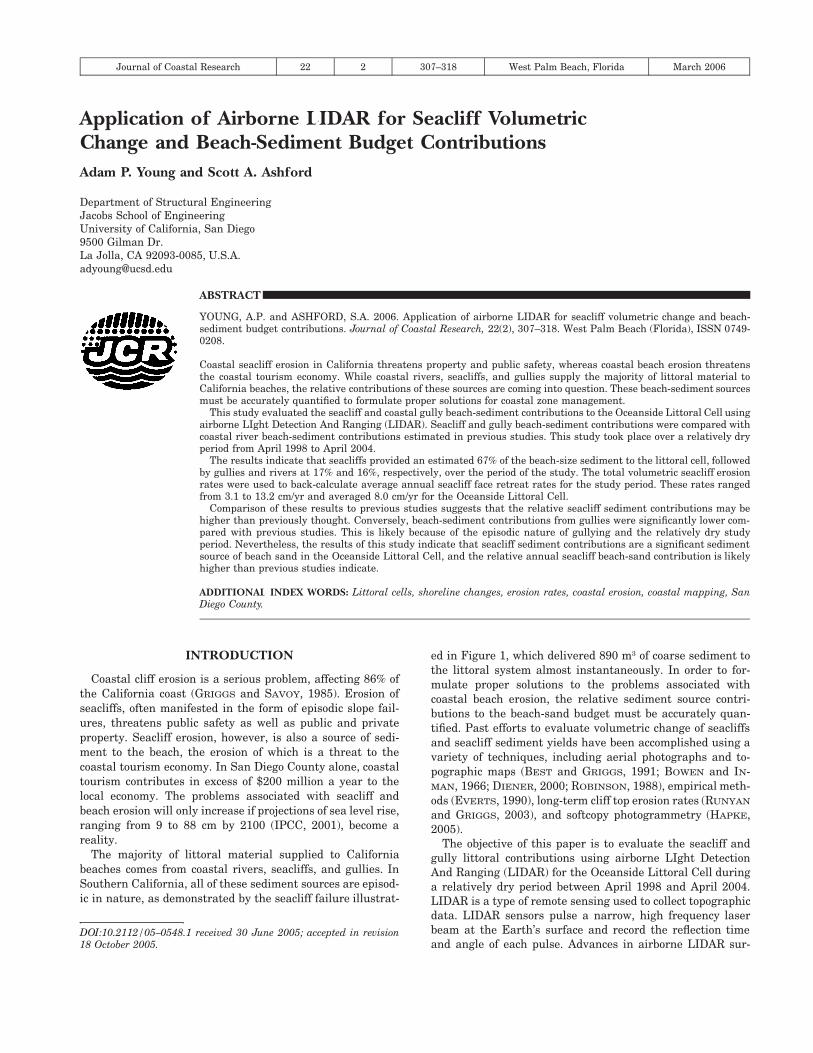
Application of Airborne LIDAR for Seacliff Volumetric ...cdip.ucsd.edu/SCBPS/DOCS/Publications/Article/Young_and_Ashford...Application of Airborne LIDAR for Seacliff Volumetric Change

Journal of Coastal Research 22 2 307–318 West Palm Beach, Florida March 2006

Application of Airborne LIDAR for Seacliff VolumetricChange and Beach-Sediment Budget ContributionsAdam P. Young and Scott A. Ashford

Department of Structural EngineeringJacobs School of EngineeringUniversity of California, San Diego9500 Gilman Dr.La Jolla, CA 92093-0085, [email protected]

ABSTRACT

YOUNG, A.P. and ASHFORD, S.A. 2006. Application of airborne LIDAR for seacliff volumetric change and beach-sediment budget contributions. Journal of Coastal Research, 22(2), 307–318. West Palm Beach (Florida), ISSN 0749-0208.

Coastal seacliff erosion in California threatens property and public safety, whereas coastal beach erosion threatensthe coastal tourism economy. While coastal rivers, seacliffs, and gullies supply the majority of littoral material toCalifornia beaches, the relative contributions of these sources are coming into question. These beach-sediment sourcesmust be accurately quantified to formulate proper solutions for coastal zone management.

This study evaluated the seacliff and coastal gully beach-sediment contributions to the Oceanside Littoral Cell usingairborne LIght Detection And Ranging (LIDAR). Seacliff and gully beach-sediment contributions were compared withcoastal river beach-sediment contributions estimated in previous studies. This study took place over a relatively dryperiod from April 1998 to April 2004.

The results indicate that seacliffs provided an estimated 67% of the beach-size sediment to the littoral cell, followedby gullies and rivers at 17% and 16%, respectively, over the period of the study. The total volumetric seacliff erosionrates were used to back-calculate average annual seacliff face retreat rates for the study period. These rates rangedfrom 3.1 to 13.2 cm/yr and averaged 8.0 cm/yr for the Oceanside Littoral Cell.

Comparison of these results to previous studies suggests that the relative seacliff sediment contributions may behigher than previously thought. Conversely, beach-sediment contributions from gullies were significantly lower com-pared with previous studies. This is likely because of the episodic nature of gullying and the relatively dry studyperiod. Nevertheless, the results of this study indicate that seacliff sediment contributions are a significant sedimentsource of beach sand in the Oceanside Littoral Cell, and the relative annual seacliff beach-sand contribution is likelyhigher than previous studies indicate.

ADDITIONAL INDEX WORDS: Littoral cells, shoreline changes, erosion rates, coastal erosion, coastal mapping, SanDiego County.

INTRODUCTION

Coastal cliff erosion is a serious problem, affecting 86% ofthe California coast (GRIGGS and SAVOY, 1985). Erosion ofseacliffs, often manifested in the form of episodic slope fail-ures, threatens public safety as well as public and privateproperty. Seacliff erosion, however, is also a source of sedi-ment to the beach, the erosion of which is a threat to thecoastal tourism economy. In San Diego County alone, coastaltourism contributes in excess of $200 million a year to thelocal economy. The problems associated with seacliff andbeach erosion will only increase if projections of sea level rise,ranging from 9 to 88 cm by 2100 (IPCC, 2001), become areality.

The majority of littoral material supplied to Californiabeaches comes from coastal rivers, seacliffs, and gullies. InSouthern California, all of these sediment sources are episod-ic in nature, as demonstrated by the seacliff failure illustrat-

DOI:10.2112/05–0548.1 received 30 June 2005; accepted in revision18 October 2005.

ed in Figure 1, which delivered 890 m3 of coarse sediment tothe littoral system almost instantaneously. In order to for-mulate proper solutions to the problems associated withcoastal beach erosion, the relative sediment source contri-butions to the beach-sand budget must be accurately quan-tified. Past efforts to evaluate volumetric change of seacliffsand seacliff sediment yields have been accomplished using avariety of techniques, including aerial photographs and to-pographic maps (BEST and GRIGGS, 1991; BOWEN and IN-MAN, 1966; DIENER, 2000; ROBINSON, 1988), empirical meth-ods (EVERTS, 1990), long-term cliff top erosion rates (RUNYAN

and GRIGGS, 2003), and softcopy photogrammetry (HAPKE,2005).

The objective of this paper is to evaluate the seacliff andgully littoral contributions using airborne LIght DetectionAnd Ranging (LIDAR) for the Oceanside Littoral Cell duringa relatively dry period between April 1998 and April 2004.LIDAR is a type of remote sensing used to collect topographicdata. LIDAR sensors pulse a narrow, high frequency laserbeam at the Earth’s surface and record the reflection timeand angle of each pulse. Advances in airborne LIDAR sur-

308 Young and Ashford

Journal of Coastal Research, Vol. 22, No. 2, 2006

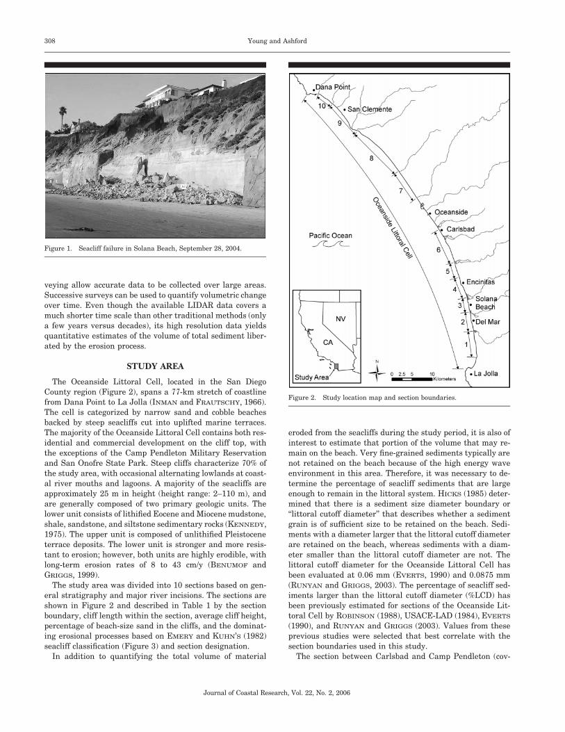
Figure 1. Seacliff failure in Solana Beach, September 28, 2004.

Figure 2. Study location map and section boundaries.

veying allow accurate data to be collected over large areas.Successive surveys can be used to quantify volumetric changeover time. Even though the available LIDAR data covers amuch shorter time scale than other traditional methods (onlya few years versus decades), its high resolution data yieldsquantitative estimates of the volume of total sediment liber-ated by the erosion process.

STUDY AREA

The Oceanside Littoral Cell, located in the San DiegoCounty region (Figure 2), spans a 77-km stretch of coastlinefrom Dana Point to La Jolla (INMAN and FRAUTSCHY, 1966).The cell is categorized by narrow sand and cobble beachesbacked by steep seacliffs cut into uplifted marine terraces.The majority of the Oceanside Littoral Cell contains both res-idential and commercial development on the cliff top, withthe exceptions of the Camp Pendleton Military Reservationand San Onofre State Park. Steep cliffs characterize 70% ofthe study area, with occasional alternating lowlands at coast-al river mouths and lagoons. A majority of the seacliffs areapproximately 25 m in height (height range: 2–110 m), andare generally composed of two primary geologic units. Thelower unit consists of lithified Eocene and Miocene mudstone,shale, sandstone, and siltstone sedimentary rocks (KENNEDY,1975). The upper unit is composed of unlithified Pleistoceneterrace deposits. The lower unit is stronger and more resis-tant to erosion; however, both units are highly erodible, withlong-term erosion rates of 8 to 43 cm/y (BENUMOF andGRIGGS, 1999).

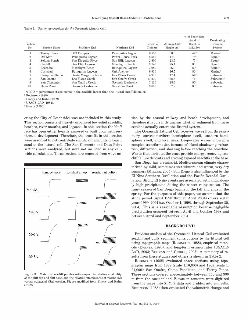
The study area was divided into 10 sections based on gen-eral stratigraphy and major river incisions. The sections areshown in Figure 2 and described in Table 1 by the sectionboundary, cliff length within the section, average cliff height,percentage of beach-size sand in the cliffs, and the dominat-ing erosional processes based on EMERY and KUHN’S (1982)seacliff classification (Figure 3) and section designation.

In addition to quantifying the total volume of material

eroded from the seacliffs during the study period, it is also ofinterest to estimate that portion of the volume that may re-main on the beach. Very fine-grained sediments typically arenot retained on the beach because of the high energy waveenvironment in this area. Therefore, it was necessary to de-termine the percentage of seacliff sediments that are largeenough to remain in the littoral system. HICKS (1985) deter-mined that there is a sediment size diameter boundary or‘‘littoral cutoff diameter’’ that describes whether a sedimentgrain is of sufficient size to be retained on the beach. Sedi-ments with a diameter larger that the littoral cutoff diameterare retained on the beach, whereas sediments with a diam-eter smaller than the littoral cutoff diameter are not. Thelittoral cutoff diameter for the Oceanside Littoral Cell hasbeen evaluated at 0.06 mm (EVERTS, 1990) and 0.0875 mm(RUNYAN and GRIGGS, 2003). The percentage of seacliff sed-iments larger than the littoral cutoff diameter (%LCD) hasbeen previously estimated for sections of the Oceanside Lit-toral Cell by ROBINSON (1988), USACE-LAD (1984), EVERTS

(1990), and RUNYAN and GRIGGS (2003). Values from theseprevious studies were selected that best correlate with thesection boundaries used in this study.

The section between Carlsbad and Camp Pendleton (cov-

309Quantifying Seacliff Beach-Sediment Contributions


Table 1. Section descriptions for the Oceanside Littoral Cell.

SectionNo. Section Name Southern End Northern End

Length ofCliffs (m)

Average CliffHeight (m)

% of Beach-SizeSand inSeacliffs(%LCD1)

DominatingErosionalProcess

12345

Torrey PinesDel MarSolana BeachCardiffLeucadia

SIO CampusPenaquitos LagoonSan Dieguito RiverSan Elijo LagoonMoonlight Beach

Penaquitos LagoonPower House ParkSan Elijo LagoonMoonlight BeachBataquitos Lagoon

6,5502,5502,8003,7403,980

88.017.923.525.126.0

422

754

754

804

804

Marine3

Equal3

Equal3

Equal3

Equal3

6789

10

CarlsbadCamp PendletonSan OnofreSan ClementeDana Point

Bataquitos LagoonSanta Margarita RiverLas Flores CreekSan Onofre CreekSecunda Deshecha

Oak AvenueLas Flores CreekSan Onofre CreekSecunda DeshechaSan Juan Creek

6,9104,970

11,2307,1303,830

16.517.438.628.637.2

804

542

712

805

805

Marine3

Subaerial3

Subaerial3

SubaerialSubaerial

1 %LCD 5 percentage of sediments in the seacliffs larger than the littoral cutoff diameter.2 Robinson (1988).3 Emery and Kuhn (1982).4 USACE-LAD (1984).5 Everts (1990).

Figure 3. Matrix of seacliff profiles with respect to relative erodibilityof the cliff top and cliff base, and the relative effectiveness of marine (M)versus subaerial (SA) erosion. Figure modified from Emery and Kuhn(1982).

ering the City of Oceanside) was not included in this study.This section consists of heavily urbanized low-relief seacliffs,beaches, river mouths, and lagoons. In this section the bluffface has been either heavily armored or built upon with res-idential development. Therefore, the seacliffs in this sectionwere assumed to not contribute significant amounts of beachsand to the littoral cell. The San Clemente and Data Pointsections were analyzed, but were not included in any cell-wide calculations. These sections are removed from wave ac-

tion by the coastal railway and beach development, andtherefore it is currently unclear whether sediment from thesesections actually enters the littoral system.

The Oceanside Littoral Cell receives waves from three pri-mary sources: northern hemisphere swell, southern hemi-sphere swell, and local seas. Deep-water waves undergo acomplex transformation because of island shadowing, refrac-tion, diffraction, and shoaling before reaching the coastline.Waves that arrive at the coast provide energy, removing sea-cliff failure deposits and eroding exposed seacliffs at the base.

San Diego has a semiarid, Mediterranean climate charac-terized by mild, sometimes wet winters and warm, very drysummers (MILLER, 2005). San Diego is also influenced by theEl Nino Southern Oscillation and the Pacific Decadal Oscil-lation. Strong El Nino events are associated with anomalous-ly high precipitation during the winter rainy season. Therainy season of San Diego begins in the fall and ends in thespring. For the purposes of this paper, we assume that thestudy period (April 1998 through April 2004) covers wateryears 1999–2004 (i.e., October 1, 1998, through September 30,2004). This is a reasonable assumption because negligibleprecipitation occurred between April and October 1998 andbetween April and September 2004.

BACKGROUND

Previous studies of the Oceanside Littoral Cell evaluatedseacliff and gully sediment contributions to the littoral cellusing topographic maps (ROBINSON, 1988), empirical meth-ods (EVERTS, 1990), and long-term erosion rates (USACE-LAD, 2003; RUNYAN and GRIGGS, 2003). A summary of re-sults from these studies and others is shown in Table 2.

ROBINSON (1988) evaluated three sections using topo-graphic maps from 1889 (scale 1:10,000) and 1968 (scale 1:24,000): San Onofre, Camp Pendleton, and Torrey Pines.These sections covered approximately between 450 and 900m from the coast inland. Elevation contours were digitizedfrom the maps into X, Y, Z data and gridded into 8-m cells.ROBINSON (1988) then evaluated the volumetric change and



Tab

le2.

Sum

mar

yof

annu

albe

ach-

sedi

men

tco

ntri

buti

ons

toth

eO

cean

side

Lit

tora

lC

ell

from

prev

ious

stud

ies.

Sec

tion

Sed

imen

tS

ourc

eA

ctua

lor

Nat

ural

Ann

ual

Bea

ch-S

edim

ent

Vol

umes

(m3/y

r)

Rob

inso

n(1

988)

Eve

rts

(199

0)U

SA

CE

-LA

D(2

003)

Run

yan

and

Gri

ggs

(200

3)

Wil

lis

etal

.(2

002)

Fli

ck(1

993)

Inm

anan

dM

aste

rs(2

005)

Tor

rey

Pin

esC

amp

Pen

dlet

onS

anO

nofr

eS

olan

aB

each

Car

diff

Leu

cadi

a

Sea

clif

fs,g

ulli

es,t

erra

ces

Sea

clif

fs,g

ulli

es,t

erra

ces

Sea

clif

fs,g

ulli

es,t

erra

ces

Sea

clif

fsS

eacl

iffs

Sea

clif

fs

Nat

ural

Nat

ural

Nat

ural

Act

ual

Act

ual

Act

ual

42,3

0090

,300

138,

200

— — —

— — — — — —

— — — 3184

2397

4168

— — — — — —

— — — — — —

— — — — — —

— — — — — —O

cean

side

Lit

tora

lC

ell

Oce

ansi

deL

itto

ral

Cel

lO

cean

side

Lit

tora

lC

ell

Oce

ansi

deL

itto

ral

Cel

lO

cean

side

Lit

tora

lC

ell

Oce

ansi

deL

itto

ral

Cel

lO

cean

side

Lit

tora

lC

ell

Oce

ansi

deL

itto

ral

Cel

l

Sea

clif

fsS

eacl

iffs

Gul

lies

,ter

race

sG

ulli

esT

erra

ces

Coa

stal

rive

rsC

oast

alri

vers

Coa

stal

rive

rs

Nat

ural

Act

ual

Bot

hN

atur

alN

atur

alA

ctua

lA

ctua

lN

atur

al

— — — — — — — —

32,9

00— —

296,

700

4000

— — —

— — — — — — — —

51,4

0042

,000

219,

400

— — — — —

— — — — —10

1,00

0— —

— — — — — —11

2,00

0–20

3,00

017

0,00

0–34

6,00

0

— — — — — — — —O

cean

side

Lit

tora

lC

ell

Oce

ansi

deL

itto

ral

Cel

lO

cean

side

Lit

tora

lC

ell

Coa

stal

rive

rsC

oast

alri

vers

Coa

stal

rive

rs

Act

ual

(dry

)A

ctua

l(w

et)

Act

ual

(ave

rage

)

— — —

— — —

— — —

— — —

— — —

— — —

19,1

0029

3,00

012

2,00

0 calculated the beach-sediment yield based on the %LCD ineach section.

EVERTS (1990) developed an empirical method to hindcastand forecast linear seacliff toe retreat rates for the OceansideLittoral Cell. The average annual seacliff toe retreat rateswere calculated based on the frequency probability of stormevents and associated seacliff toe retreat. The linear toe re-treat rates ranged from 1.5 to 9 cm/yr. The annual seaclifftoe retreat rates were then used to calculate the natural an-nual seacliff beach-sediment contribution (i.e., excluding theeffect of seacliff stabilization) to the littoral cell by using thefollowing general equation:

Qs 5 Lc 3 Rl 3 Hc 3 %LCD (1)

where:Qs 5 natural annual seacliff sediment yieldLc 5 length of seacliffsRl 5 linear rate of seacliff retreatHc 5 average height of seacliffs

USACE-LAD (2003) also used the general form of Equation(1) to calculate the annual sediment yields for Solana Beachand Encinitas. The average seacliff top retreat rates esti-mated by USACE-LAD (2003) ranged from 7.6 to 37.0 cm/yr.This study assumed that the cliff top would retreat to createa more stable slope, and therefore the annual beach-sedimentvolumes were reduced by one-half to account for this equilib-rium. Because shoreline protection reduces the amount of lit-toral material supplied to the beaches, the natural annualbeach-sediment contributions were adjusted downward to ac-count for the percentage of protective devices, thus resultingin the actual contribution.

RUNYAN and GRIGGS (2003) calculated natural seacliff con-tributions to the Oceanside Littoral Cell using long-term (40–60 years) seacliff top retreat rates from both BENUMOF andGRIGGS (1999) and MOORE, BENUMOF, and GRIGGS (1998).These linear seacliff top retreat rates ranged from 10 to 20cm/yr. Seacliff beach-sediment yields were then calculatedusing the general form of Equation (1). RUNYAN and GRIGGS

(2003) calculated the annual gully volume by subtractingtheir natural annual seacliff beach-sand volume from Rob-inson’s combined seacliff and gully annual beach-sand vol-ume. RUNYAN and GRIGGS (2003) also calculated the actualannual seacliff volume by reducing their natural annualbeach-sand volume based on the percentage of shoreline ar-moring in each section.

The surfaces of coastal terraces can provide beach-sand tolittoral system by means of subaerial erosion and smallstream transportation. The terrace degradation sedimentyield was estimated by EVERTS (1990) at 4000 m3/yr for theOceanside Littoral Cell. For the purposes of this study, ter-race surface yields were assumed to be negligible in the over-all sediment budget because of the dry study period and rel-atively low volume reported by EVERTS (1990).

Rivers can provide a significant amount of beach-sand tothe littoral cell. However, the natural average annual sedi-ment load of California coastal rivers has been significantlyreduced by the development of the coastal watershed throughflood control and water storage dams (BROWNLIE and TAY-



LOR, 1981; FLICK, 1993; GRIGGS, 1987; INMAN and BRUSH,1973; INMAN and JENKINS, 1999; WILLIS, SHERMAN, andLOCKWOOD, 2002). These studies indicate that the naturalbeach-sediment load of coastal rivers in the Oceanside Lit-toral Cell has been reduced by approximately one half. FLICK

(1993) summarized several studies that estimate the actuallong-term average annual coastal river beach-sediment fluxto the Oceanside Littoral Cell at 112,000–203,000 m3/yr. Amore recent study by WILLIS, SHERMAN, and LOCKWOOD

(2002) estimates the actual beach-sediment flux at 101,000m3/yr. It should be noted that the fluvial beach-sediment de-livery to the littoral system is highly episodic in California.INMAN and JENKINS (1999) found that the average annualsediment flux during wet periods is five times higher com-pared to dry periods for California rivers, and that this epi-sodicity is even more pronounced in Southern California. Infact, INMAN and MASTERS (2005) estimate the fluvial beach-sand flux in the Oceanside Littoral Cell for dry and wet pe-riods at 19,100 m3/yr and 293,000 m3/yr respectively, whichis approximately a 15 times difference for wet and dry peri-ods.

Based on the studies presented above, the total annualamount of beach-sediment contribution from all naturalsources combined (rivers, seacliffs, gullies, and terraces)would appear to range from just over 350,000 m3/yr to nearly550,000 m3/yr. Of this total, the contribution of seacliff ero-sion is on the order of 10 to 15 percent, which is in agreementwith conventional wisdom, whereas gully erosion appears tobe the most significant source of beach sediment. It shouldbe noted, however, that the contributions of gullies noted inEVERTS (1990) and RUNYAN and GRIGGS (2003) are directlyrelated to the initial estimates of ROBINSON (1988). The datapresented by ROBINSON (1988) is based on interpretation ofold topographic maps and dominated by a limited number ofextreme gully erosion events caused by altered drainage pat-terns associated with the construction of coastal highways inthe Camp Pendleton and San Onofre sections. KUHN andSHEPARD (1984) documented several of these events, includ-ing the formation of a new canyon in the San Onofre section,which eroded landward 140 meters between 1968 and 1980,and Dead Dog Canyon in the Camp Pendleton section, whicheroded landward 230 meters between 1932 and 1980. Below,we use airborne LIDAR data to quantify the combined con-tributions of seacliffs and gullies over the 6-year study periodas an independent benchmark of the conventional wisdom,and then compare the LIDAR-developed contributions to es-timates of river beach-sediment contributions for the studyperiod.

METHODS

Topographic Change

In order to evaluate the topographic change of the seacliffs,two airborne LIDAR data sets were used that span a 6-yeartime period. The older data set was collected in April 1998using NASA’s Airborne Topographic Mapper (ATM, 1998).This survey was obtained from NOAA (2004). The seconddata set was collected in April 2004. This data set was pro-vided by the Southern California Beach Processes Study, op-

erated by the Scripps Institution of Oceanography. Both datasets were obtained in X, Y, Z format. The original point den-sities of the 1998 and 2004 data were 0.9 and 3.3 points perm2, respectively. The X, Y, Z point data were interpolated into0.5-m resolution grids using the ArcINFO 3-D Analyst (Ver-sion 9.0, 2004, Environmental Earth Science Research Insti-tute, Redlands, CA). Grid interpolation was completed usinginverse distance weighting.

After grid interpolation, the Oceanside Littoral Cell wasdivided into 10 sections for analysis. The change in elevationwas evaluated for each section by subtracting the 2004 gridfrom the 1998 grid (Equation [2]). This procedure results ina grid showing the change in elevation over time. Negativecells indicate erosion and positive cells indicate accretion.

ZChange 5 Z1998 2 Z2004 (2)

where:ZChange 5 cell change in elevationZ2004 5 cell elevation in 2004Z1998 5 cell elevation in 1998

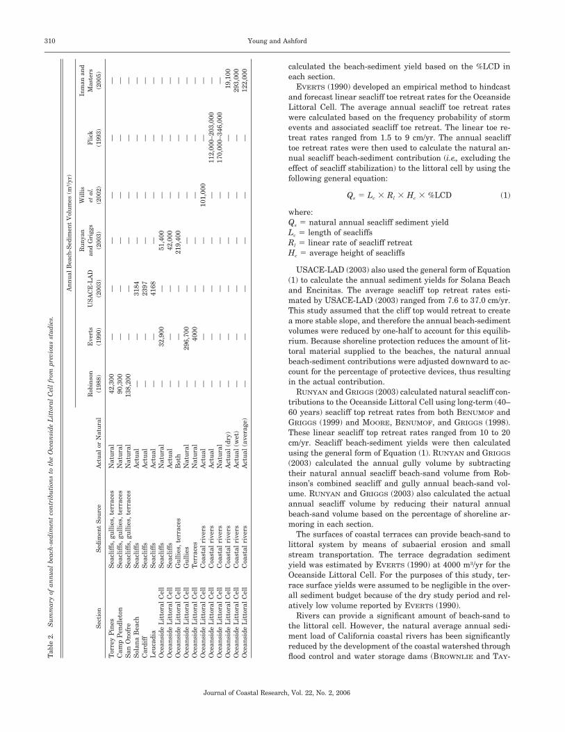
Figure 4 shows the central portion of the Solana Beach griddisplayed under a transparent shaded relief. The red areasin this figure indicate areas where significant erosion oc-curred during the study period. This figure shows numerousdistinct upper seacliff failures as well as several sections oflower seacliff retreat. These calculations were performed us-ing data from the base of the 1998 seacliff landward. Nochanges in beach volumes are included.

The potential error in the change grid can be primarilyattributed to LIDAR measurement error, interpolation error,and vegetation. Error evaluation was done by computing theroot mean square (RMS), which describes the average mag-nitude of change between the two data sets. Typical verticalRMS error for quantifying beach changes using airborne to-pographic LIDAR is 15 cm (SALLENGER et al., 2003). ThisRMS value was not deemed to accurately quantify the errorin this study, because it focused on high relief cliffs with par-tial vegetation in some areas. Therefore the RMS error wasevaluated using a 400-m representative control section in En-cinitas between Swami’s and San Elijo State Beach. The con-trol section consists of a partially vegetated slope and wasassumed to have no significant change over the time period,because it was stabilized in 1960 using a rock revetment atthe base, slope grading, and surface drainage control (KUHN

and SHEPARD, 1984). The vertical RMS for this section wascalculated using Equation (3) (FEDERAL GEOGRAPHIC DATA

COMMITTEE, 1998).

n2(za 2 zb )O i i

i51ÎRMS 5 (3)Z n

where:zai 5 cell elevation in 2004zbi 5 cell elevation in 1998n 5 number of cells

The RMSZ of the control section was calculated at 21 cm.This value was then used as a threshold of acceptable error



Figure 4. Erosion grid of central Solana Beach where red cells representseacliff erosion that occurred between April 1998 and April 2004. Severalupper cliff failures and sections of lower cliff retreat are shown in thisfigure.

Table 3. Section error.

Section Name RMS (m) Error (%)

Test sectionTorrey PinesDel MarSolana BeachCardiffLeucadiaCarlsbadCamp PendletonSan OnofreSan ClementeDana PointOceanside Littoral Cell

0.211.281.072.121.201.320.810.751.431.421.311.32

—16.4 (6 8.2)19.7 (6 9.9)9.9 (6 5.0)

17.5 (6 8.8)15.9 (6 8.0)25.9 (6 13.0)28.1 (6 4.1)14.6 (6 7.3)14.7 (6 7.4)16.0 (6 8.0)16.0 (6 8.0)

for each cell. Each cliff section was isolated from the beachand cliff top development by clipping the change grids alongthe seacliff base and cliff top. Next, cells that showed erosionof 21 cm or more (2` , cells , 221 cm from Equation [2])were extracted from each section to produce a new erosion-only grid.

RMSZ values were then calculated for each erosion grid.Statistical error for each section was calculated as a ratiobased on the RMSZ of the control section, using Equation (4)(ZHANG et al., 2005). Table 3 summarizes the RMSZ and per-centage error for each section and weighted cell average.

Percentage Error 5 RMS /RMS (4)Z(Control Section) Z(Seacliff Section)

Other error in the grids may have come from interpolatingover sharp edges or vegetation. Aerial LIDAR typically doesnot capture over vertical surfaces such as seacaves or notch-es. Therefore, changes that occurred in these areas were notevaluated. Complete LIDAR coverage was not available forLas Pulgas Canyon and a small portion of the Torrey Pinessection, and these areas were also not evaluated.

The total eroded volumes were calculated for each sectionby summing the volumes of negative cells less than thethreshold value of 221 cm. Cells that showed erosion valuesbetween 0 and 221 cm were removed to compensate for pos-sible grid interpolation error.

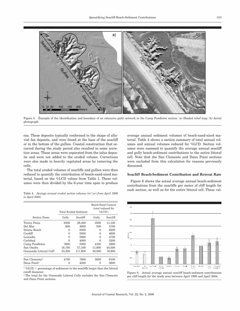
Gullies were clipped out of the erosion grids to quantify theeroded gully volume. Gullies were removed from the totalseacliff eroded volume because, although they did contributebeach sediment to the littoral cell, they did not contribute tothe eroded volume of the seacliff face. Gullies in each sectionwere identified using the generated digital elevation modelsand aerial photographs. For this project, gullies were definedas areas where significant subaerial erosion occurred becauseof concentrated terrace runoff and piping. These included ex-tensive gully networks, coastal ravines, and canyons. An ex-ample of a well-developed gully network is shown in Figure5. Subtracting the gully volumes from the total eroded vol-ume in each section produced a seacliff erosion volume.

Areas that showed significant accretion and were deter-mined to be landslide talus deposits were added to the erodedvolume for correction. These volumes were added back in tothe corresponding seacliff or gully section because they hadnot yet entered the littoral system. Talus deposits were iden-tified as accretion areas found below significantly eroded ar-



Figure 5. Example of the identification and boundary of an extensive gully network in the Camp Pendleton section. (a) Shaded relief map. (b) Aerialphotograph.

Table 4. Average annual eroded section volumes (m3/yr) from April 1998to April 2004.

Section Name

Total Eroded Sediment

Gully Seacliff

Beach-Sand Content(total reduced for

%LCD1)

Gully Seacliff

Torrey PinesDel MarSolana BeachCardiffLeucadiaCarlsbadCamp PendletonSan OnofreOceanside Littoral Cell2

8300600

0000

760016,70033,200

26,400490083005800590040005500

57,100117,900

3500500

0000

410011,90020,000

11,100370062004600470032002900

40,50076,900

San Clemente2

Dana Point2

47000

76004500

38000

61003600

1 %LCD 5 percentage of sediments in the seacliffs larger than the littoralcutoff diameter.2 The total for the Oceanside Littoral Cells excludes the San Clementeand Dana Point sections.

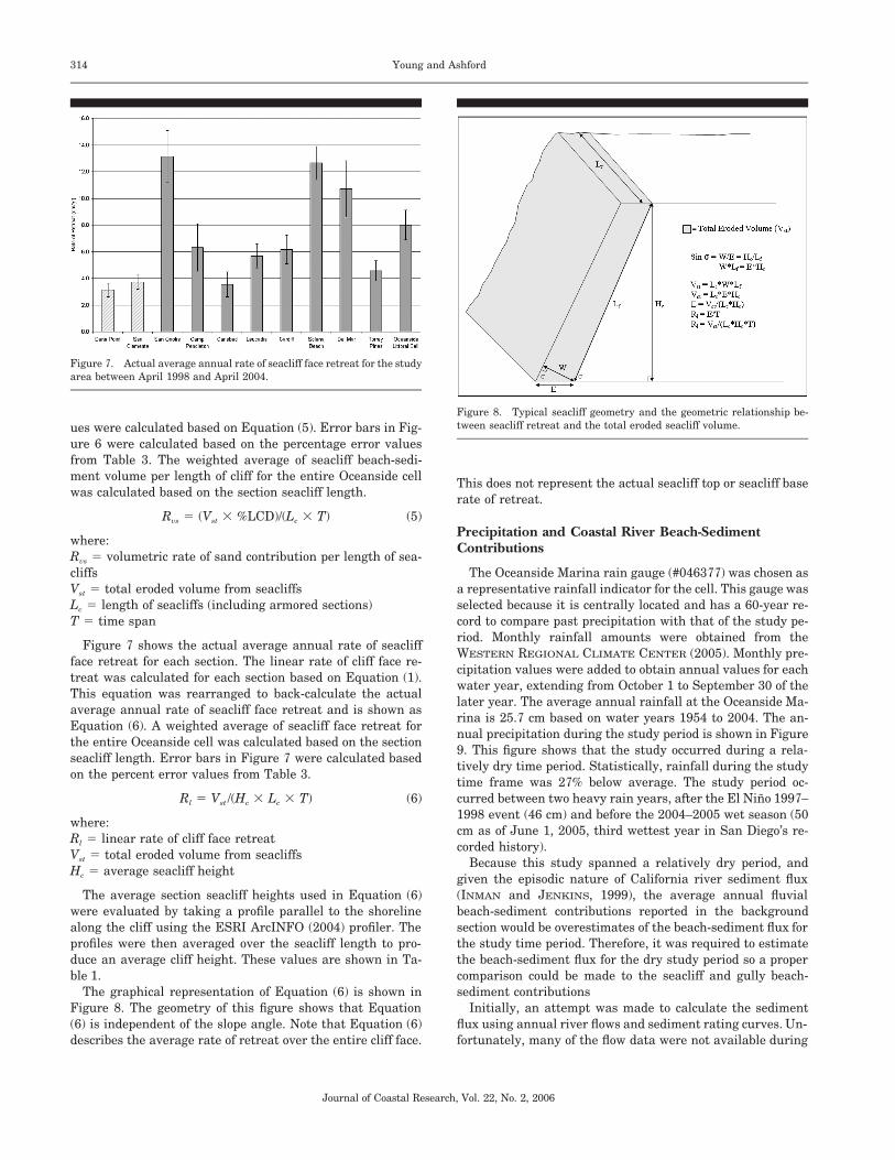
Figure 6. Actual average annual seacliff beach-sediment contributionsper cliff length for the study area between April 1998 and April 2004.

eas. These deposits typically conformed to the shape of allu-vial fan deposits, and were found at the base of the seacliffor in the bottom of the gullies. Coastal construction that oc-curred during the study period also resulted in some accre-tion areas. These areas were separated from the talus depos-its and were not added to the eroded volume. Correctionswere also made in heavily vegetated areas by removing thecells.

The total eroded volumes of seacliffs and gullies were thenreduced to quantify the contribution of beach-sand-sized ma-terial, based on the %LCD values from Table 1. These vol-umes were then divided by the 6-year time span to produce

average annual sediment volumes of beach-sand-sized ma-terial. Table 4 shows a section summary of total annual vol-umes and annual volumes reduced for %LCD. Section vol-umes were summed to quantify the average annual seacliffand gully beach-sediment contributions to the entire littoralcell. Note that the San Clemente and Dana Point sectionswere excluded from this calculation for reasons previouslydiscussed.

Seacliff Beach-Sediment Contribution and Retreat Rate

Figure 6 shows the actual average annual beach-sedimentcontributions from the seacliffs per meter of cliff length foreach section, as well as for the entire littoral cell. These val-



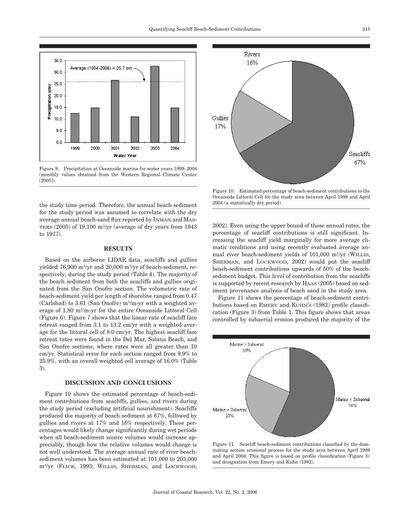
Figure 7. Actual average annual rate of seacliff face retreat for the studyarea between April 1998 and April 2004.

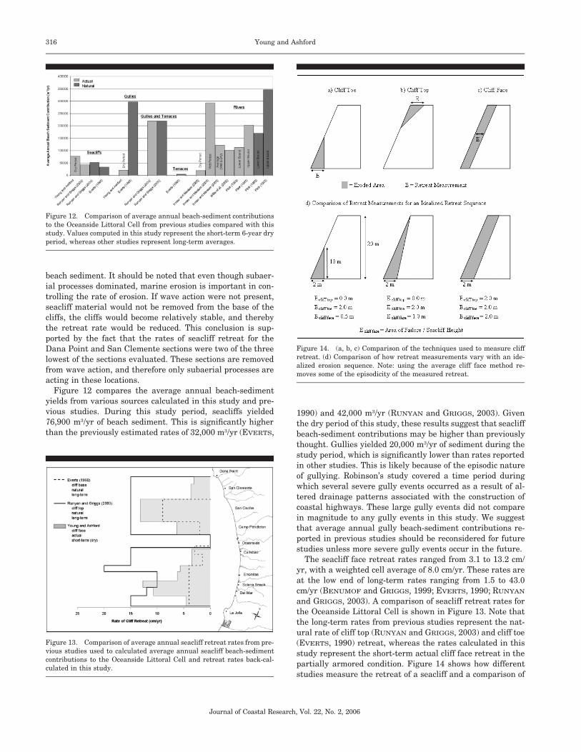
Figure 8. Typical seacliff geometry and the geometric relationship be-tween seacliff retreat and the total eroded seacliff volume.ues were calculated based on Equation (5). Error bars in Fig-

ure 6 were calculated based on the percentage error valuesfrom Table 3. The weighted average of seacliff beach-sedi-ment volume per length of cliff for the entire Oceanside cellwas calculated based on the section seacliff length.

Rvs 5 (Vst 3 %LCD)/(Lc 3 T) (5)

where:Rvs 5 volumetric rate of sand contribution per length of sea-cliffsVst 5 total eroded volume from seacliffsLc 5 length of seacliffs (including armored sections)T 5 time span

Figure 7 shows the actual average annual rate of seacliffface retreat for each section. The linear rate of cliff face re-treat was calculated for each section based on Equation (1).This equation was rearranged to back-calculate the actualaverage annual rate of seacliff face retreat and is shown asEquation (6). A weighted average of seacliff face retreat forthe entire Oceanside cell was calculated based on the sectionseacliff length. Error bars in Figure 7 were calculated basedon the percent error values from Table 3.

Rl 5 Vst /(Hc 3 Lc 3 T) (6)

where:Rl 5 linear rate of cliff face retreatVst 5 total eroded volume from seacliffsHc 5 average seacliff height

The average section seacliff heights used in Equation (6)were evaluated by taking a profile parallel to the shorelinealong the cliff using the ESRI ArcINFO (2004) profiler. Theprofiles were then averaged over the seacliff length to pro-duce an average cliff height. These values are shown in Ta-ble 1.

The graphical representation of Equation (6) is shown inFigure 8. The geometry of this figure shows that Equation(6) is independent of the slope angle. Note that Equation (6)describes the average rate of retreat over the entire cliff face.

This does not represent the actual seacliff top or seacliff baserate of retreat.

Precipitation and Coastal River Beach-SedimentContributions

The Oceanside Marina rain gauge (#046377) was chosen asa representative rainfall indicator for the cell. This gauge wasselected because it is centrally located and has a 60-year re-cord to compare past precipitation with that of the study pe-riod. Monthly rainfall amounts were obtained from theWESTERN REGIONAL CLIMATE CENTER (2005). Monthly pre-cipitation values were added to obtain annual values for eachwater year, extending from October 1 to September 30 of thelater year. The average annual rainfall at the Oceanside Ma-rina is 25.7 cm based on water years 1954 to 2004. The an-nual precipitation during the study period is shown in Figure9. This figure shows that the study occurred during a rela-tively dry time period. Statistically, rainfall during the studytime frame was 27% below average. The study period oc-curred between two heavy rain years, after the El Nino 1997–1998 event (46 cm) and before the 2004–2005 wet season (50cm as of June 1, 2005, third wettest year in San Diego’s re-corded history).

Because this study spanned a relatively dry period, andgiven the episodic nature of California river sediment flux(INMAN and JENKINS, 1999), the average annual fluvialbeach-sediment contributions reported in the backgroundsection would be overestimates of the beach-sediment flux forthe study time period. Therefore, it was required to estimatethe beach-sediment flux for the dry study period so a propercomparison could be made to the seacliff and gully beach-sediment contributions

Initially, an attempt was made to calculate the sedimentflux using annual river flows and sediment rating curves. Un-fortunately, many of the flow data were not available during



Figure 9. Precipitation at Oceanside marina for water years 1999–2004(monthly values obtained from the Western Regional Climate Center[2005]).

Figure 10. Estimated percentage of beach-sediment contributions to theOceanside Littoral Cell for the study area between April 1998 and April2004 (a statistically dry period).

Figure 11. Seacliff beach-sediment contributions classified by the dom-inating section erosional process for the study area between April 1998and April 2004. This figure is based on profile classification (Figure 3)and designation from Emery and Kuhn (1982).

the study time period. Therefore, the annual beach sedimentfor the study period was assumed to correlate with the dryaverage annual beach-sand flux reported by INMAN and MAS-TERS (2005) of 19,100 m3/yr (average of dry years from 1943to 1977).

RESULTS

Based on the airborne LIDAR data, seacliffs and gulliesyielded 76,900 m3/yr and 20,000 m3/yr of beach-sediment, re-spectively, during the study period (Table 4). The majority ofthe beach sediment from both the seacliffs and gullies origi-nated from the San Onofre section. The volumetric rate ofbeach-sediment yield per length of shoreline ranged from 0.47(Carlsbad) to 3.61 (San Onofre) m3/m-yr with a weighted av-erage of 1.80 m3/m-yr for the entire Oceanside Littoral Cell(Figure 6). Figure 7 shows that the linear rate of seacliff faceretreat ranged from 3.1 to 13.2 cm/yr with a weighted aver-age for the littoral cell of 8.0 cm/yr. The highest seacliff faceretreat rates were found in the Del Mar, Solana Beach, andSan Onofre sections, where rates were all greater than 10cm/yr. Statistical error for each section ranged from 9.9% to25.9%, with an overall weighted cell average of 16.0% (Table3).

DISCUSSION AND CONCLUSIONS

Figure 10 shows the estimated percentage of beach-sedi-ment contributions from seacliffs, gullies, and rivers duringthe study period (excluding artificial nourishment). Seacliffsproduced the majority of beach sediment at 67%, followed bygullies and rivers at 17% and 16% respectively. These per-centages would likely change significantly during wet periodswhen all beach-sediment source volumes would increase ap-preciably, though how the relative volumes would change isnot well understood. The average annual rate of river beach-sediment volumes has been estimated at 101,000 to 203,000m3/yr (FLICK, 1993; WILLIS, SHERMAN, and LOCKWOOD,

2002). Even using the upper bound of these annual rates, thepercentage of seacliff contributions is still significant. In-creasing the seacliff yield marginally for more average cli-matic conditions and using recently evaluated average an-nual river beach-sediment yields of 101,000 m3/yr (WILLIS,SHERMAN, and LOCKWOOD, 2002) would put the seacliffbeach-sediment contributions upwards of 50% of the beach-sediment budget. This level of contribution from the seacliffsis supported by recent research by HAAS (2005) based on sed-iment provenance analysis of beach sand in the study area.

Figure 11 shows the percentage of beach-sediment contri-butions based on EMERY and KUHN’S (1982) profile classifi-cation (Figure 3) from Table 1. This figure shows that areascontrolled by subaerial erosion produced the majority of the



Figure 12. Comparison of average annual beach-sediment contributionsto the Oceanside Littoral Cell from previous studies compared with thisstudy. Values computed in this study represent the short-term 6-year dryperiod, whereas other studies represent long-term averages.

Figure 14. (a, b, c) Comparison of the techniques used to measure cliffretreat. (d) Comparison of how retreat measurements vary with an ide-alized erosion sequence. Note: using the average cliff face method re-moves some of the episodicity of the measured retreat.

Figure 13. Comparison of average annual seacliff retreat rates from pre-vious studies used to calculated average annual seacliff beach-sedimentcontributions to the Oceanside Littoral Cell and retreat rates back-cal-culated in this study.

beach sediment. It should be noted that even though subaer-ial processes dominated, marine erosion is important in con-trolling the rate of erosion. If wave action were not present,seacliff material would not be removed from the base of thecliffs, the cliffs would become relatively stable, and therebythe retreat rate would be reduced. This conclusion is sup-ported by the fact that the rates of seacliff retreat for theDana Point and San Clemente sections were two of the threelowest of the sections evaluated. These sections are removedfrom wave action, and therefore only subaerial processes areacting in these locations.

Figure 12 compares the average annual beach-sedimentyields from various sources calculated in this study and pre-vious studies. During this study period, seacliffs yielded76,900 m3/yr of beach sediment. This is significantly higherthan the previously estimated rates of 32,000 m3/yr (EVERTS,

1990) and 42,000 m3/yr (RUNYAN and GRIGGS, 2003). Giventhe dry period of this study, these results suggest that seacliffbeach-sediment contributions may be higher than previouslythought. Gullies yielded 20,000 m3/yr of sediment during thestudy period, which is significantly lower than rates reportedin other studies. This is likely because of the episodic natureof gullying. Robinson’s study covered a time period duringwhich several severe gully events occurred as a result of al-tered drainage patterns associated with the construction ofcoastal highways. These large gully events did not comparein magnitude to any gully events in this study. We suggestthat average annual gully beach-sediment contributions re-ported in previous studies should be reconsidered for futurestudies unless more severe gully events occur in the future.

The seacliff face retreat rates ranged from 3.1 to 13.2 cm/yr, with a weighted cell average of 8.0 cm/yr. These rates areat the low end of long-term rates ranging from 1.5 to 43.0cm/yr (BENUMOF and GRIGGS, 1999; EVERTS, 1990; RUNYAN

and GRIGGS, 2003). A comparison of seacliff retreat rates forthe Oceanside Littoral Cell is shown in Figure 13. Note thatthe long-term rates from previous studies represent the nat-ural rate of cliff top (RUNYAN and GRIGGS, 2003) and cliff toe(EVERTS, 1990) retreat, whereas the rates calculated in thisstudy represent the short-term actual cliff face retreat in thepartially armored condition. Figure 14 shows how differentstudies measure the retreat of a seacliff and a comparison of



the measured retreat for an idealized erosion sequence. Thisfigure shows how it is critical to understand where the re-treat is being measured and why retreat rates may not bedirectly comparable. This figure also shows how using thecliff face retreat measurement as described in this study av-erages the failure area over the cliff face, thereby removingsome of the episodic nature of retreat measurements. Com-parison of the retreat measurements through the retreat cy-cle shows that the three measurement techniques are notequal until the erosion cycle has been completed. It shouldbe noted that the retreat rates calculated in this study wereaveraged over the entire cliff section, including armored ar-eas. Therefore, the natural rate of retreat would be signifi-cantly higher in heavily armored sections. The relatively lowrates found in this study are likely because of the partiallyarmored condition and the dry climate study period.

A comparison of the average annual seacliff beach-sedi-ment yields and cliff retreat rates from this study, EVERTS

(1990), and RUNYAN and GRIGGS (2003) reveals a discrep-ancy. Because all of these studies used the same general formof Equation (1), the retreat rates and beach-sediment vol-umes should correlate in size with one another. This is notthe case; the beach-sediment volume calculated in this studyis larger than that reported by RUNYAN and GRIGGS (2003),yet the retreat rate of this study is smaller than RUNYAN andGRIGGS (2003). The main reason for this discrepancy comesfrom the significant differences in cliff height used by thisstudy and RUNYAN and GRIGGS (2003).

Given the relatively short study time period and the epi-sodic nature of cliff failures, it is difficult to make any long-term conclusions. The seacliff and gully beach-sediment con-tributions could be viewed as lower bounds, given the rela-tively dry climate of the study period. Nevertheless, the re-sults of this study indicate that seacliff beach-sedimentcontributions are a significant beach-sand source in theOceanside Littoral Cell. This study also suggests that the rel-ative seacliff beach-sand contribution may be significantlyhigher because of a possible overestimation of annual gullybeach-sand contributions for current conditions.

This study also demonstrates that airborne LIDAR analy-sis can be used to quantify seacliff and gully beach-sedimentcontributions on a large scale. Further research should beconducted to quantify volumetric changes during wet periods.A comparison of dry and wet time periods could be used toquantify the episodic nature of seacliff retreat. Additional re-search should also be conducted to more accurately quantifythe effects of marine versus subaerial erosion processes. Nowthat a baseline for the Oceanside Littoral Cell has been es-tablished, future airborne LIDAR scanning can be used toevaluate the longer term rates of seacliff erosion.

ACKNOWLEDGMENTS

This publication was supported in part by the National SeaGrant College Program of the US Department of Commerce’sNational Oceanic and Atmospheric Administration underNOAA Grant NA06RG0142, project R/OE-37, through theCalifornia Sea Grant College Program, and in part by theCalifornia State Resources Agency. Additional support was

provided by the University of California, Coastal Environ-mental Quality Initiative Program, under Award 04-T-CEQI-06-0046. In addition, the authors would like to acknowledgeand sincerely thank Richard Seymour, Robert Guza, JulieThomas, and Randy Bucciarelli of the Southern CaliforniaBeach Processes Study, operated by the Scripps Institutionof Oceanography under the sponsorship of the US ArmyCorps of Engineers and the California Department of Boatingand Waterways, for providing the 2004 LIDAR data set.Without their collaboration, this research effort would nothave been possible.

LITERATURE CITED

ATM (AIRBORNE TOPOGRAPHIC MAPPER), 1998. West Coast LIDAR.Partners: National Oceanic and Atmospheric Administration(NOAA) Coastal Services Center, the NASA Wallops Flight Facil-ity, the U. S. Geological Survey (USGS) Center for Coastal andRegional Marine Geology, and the NOAA Aircraft Operations Cen-ter.

BENUMOF, B.T. and GRIGGS, G.B., 1999. The relationship betweenseacliff erosion rates, cliff material properties, and physical pro-cesses. Shore and Beach, 67(4), 29–41.

BEST, T.C. and GRIGGS, G. B., 1991. A sediment budget for the SantaCruz littoral cell. Society of Economic Paleontologists and Miner-alogists, Special Publication No. 46, pp. 35–50.

BOWEN, A.J. and INMAN, D.L., 1966. Budget of Littoral Sands in theVicinity of Point Arguello, California. U.S. Army Coastal Engi-neering Research Center.

BROWNLIE, W.R. and TAYLOR, B.D., 1981. Sediment Managementfor the Southern California Mountains, Coastal Plains, and Shore-line, Part C: Coastal Sediment Delivery by Major Rivers in South-ern California. California Institute of Technology, EnvironmentalQuality Lab Report No. 17-C, February 1981.

DIENER, B.G, 2000. Sand contribution from bluff recession betweenPoint Conception and Santa Barbara, California. Shore and Beach,68(2), 7–14.

EMERY, K.O. and KUHN, G.G., 1982. Sea cliffs: their processes, pro-files, and classification. Geological Society of America Bulletin, 93,644–654.

EVERTS, C.H., 1990. Sediment budget report, Oceanside LittoralCell. Coast of California Storm and Tidal Wave Study 90–2, U.S.Army Corps of Engineers, Los Angeles District. 110p.

FEDERAL GEOGRPAHIC DATA COMMITTEE, 1998. Geospatial posi-tioning accuracy standards. FGDC-STD-007.3–1998, 28p.

FLICK, R.E., 1993. The myth and reality of southern Californiabeaches. Shore and Beach, 61(3), 3–13.

GRIGGS, G.B., 1987. The production, transport, and delivery ofcoarse-grained sediment by California’s coastal streams. Proceed-ings of Coastal Sediments ’87, Vol. 2. New York: American Societyof Civil Engineers, pp. 1825–1838.

GRIGGS, G.B. and SAVOY, L., (ed.), 1985. Living with the CaliforniaCoast. Durham, North Carolina: Duke University Press, 393p.

HAAS, J.K., 2005. Grain Size and Mineralogical Characteristics ofBeach Sand in the Oceanside Littoral Cell: Implications of Sedi-ment Provenance. San Diego, California: University of CaliforniaSan Diego, Master’s thesis, 41p.

HAPKE, C.J., 2005. Estimation of regional material yield from coast-al landslides based on historical digital terrain modeling. EarthSurfaces Processes and Landforms, 30(6), 679–697.

HICKS, D.M. 1985. Sand Dispersion from an Ephemeral Delta on aWave-Dominated Coast. Ph.D. Dissertation, University of Califor-nia, Santa Cruz, 210p.

INMAN, D.L. and BRUSH, B.M., 1973. The coastal challenge, Science,181, 20–32.

INMAN, D.L. and FRAUTSCHY, J.D., 1966. Littoral processes and thedevelopment of shorelines. Proceedings, Coastal Engineering Spe-cialty Conference (ASCE, Santa Barbara, California), pp. 511–536.

INMAN, D.L. and JENKINS, S.A., 1999. Climate change and the epi-



sodicity of sediment flux of small California rivers. Journal of Ge-ology, volume 107, p 251–270.

INMAN, D.L. and MASTERS, P.M., 2005. Living with Coastal Change.Scripps Institution of Oceanography, University of California, SanDiego. http://coastalchange.ucsd.edu (accessed August 30, 2005).

IPCC (INTERGOVERNMENTAL PANEL ON CLIMATE CHANGE), Work-ing group I, 2001. The Scientific Basis. Contribution of WorkingGroup I to the Third Assessment Report of the IPCC. Cambridge,UK: Cambridge University Press, 873p.

KENNEDY, M.P., 1975. Geology of the San Diego metropolitan area,western area. California Division of Mines and Geology Bulletin200, 56p.

KUHN, J.P. and SHEPARD, F.P., 1984. Sea Cliffs, Beaches, and Coast-al Valleys of San Diego County: Some Amazing Histories and SomeHorrifying Implications. Berkeley, California: University of Cali-fornia Press, 193p.

MILLER, M., 2005. The Weather Guide, A Weather Information Com-panion for the Forecast Area of the National Weather Service in SanDiego, 3rd Edition. San Diego: National Weather Service, 116p.

MOORE, L.J.; BENUMOF, B.T., and GRIGGS, G.B., 1999. Coastal ero-sion hazards in Santa Cruz and San Diego Counties, California.Journal of Coastal Research, Special Issue No. 28, pp. 121–139.

NOAA (NATIONAL OCEANIC AND ATMOSPHERIC ADMINISTRATION),2004. Coastal Services Center. http://www.csc.noaa.gov

ROBINSON, B.A., 1988. Coastal cliff sediments—San Diego region,Dana Point to the Mexican border (1887–1947). Coast of California

Storm and Tidal Wave Study 88–8. U.S. Army Corps of Engineers,Los Angeles District, 275p.

RUNYAN, K. and GRIGGS, G.B., 2003. The effect of armoring seacliffson the natural sand supply to the beaches of California. Journalof Coastal Research, 19(2), 336–347.

SALLENGER, A.H.; KRABILL, W.B.; SWIFT, R.N.; BROCK, J.; LIST, J.;HANSEN, M.; HOLMAN, R.A.; MANIZADE, S.; SONTAG, J.; MERE-DITH, A.; MORGAN, K.; YUNKEL, J.K.; FREDERICK, E.B., andSTOCKDON, H., 2003. Evaluation of airborne topographic LIDARfor quantifying beach changes. Journal of Coastal Research, 19(1),125–133.

USACE-LAD (U. S. ARMY CORPS OF ENGINEERS—LOS ANGELES

DISTRICT), 1984. Geomorphology framework report Dana Point tothe Mexican border. Coast of California Storm and Tidal WaveStudy 84–4, 101p.

USACE-LAD, 2003. Encinitas and Solana Beach Shoreline Feasibil-ity Study, San Diego County. Appendix C, 75p.

WESTERN REGIONAL CLIMATE CENTER, 2005. http://www.wrcc.dri.edu

WILLIS, C.M.; SHERMAN, D., and LOCKWOOD, B. 2002. Chapter 7:Impediments to fluvial Delivery of Sediment to the Shoreline. In:COYNE, M. and STERRETT, K. (eds.), California Beach RestorationStudy. Sacramento, California: California Boating and Waterwaysand State Coastal Conservancy, 280p.

ZHANG, K.; WHITMAN, D.; LEATHERMAN, S., and ROBERTSON, W.,2005. Quantification of beach change caused by hurricane Floydalong Florida’s Atlantic coast using airborne laser surveys. Jour-nal of Coastal Research. 21(1), 123–134.

Application of Airborne LIDAR for Seacliff Volumetric ...cdip.ucsd.edu/SCBPS/DOCS/Publications/Article/Young_and_Ashford...Application of Airborne LIDAR for Seacliff Volumetric Change

Documents