Application of a comprehensive modeling strategy for the management of net-pen aquaculture waste transport

Ž .Aquaculture 187 2000 319–349www.elsevier.nlrlocateraqua-online

Application of a comprehensive modeling strategyfor the management of net-pen aquaculture waste

transport

Robert W. Dudley a, Vijay G. Panchang b,), Carter R. Newell c

a Water Resources DiÕision, U.S. Geological SurÕey, 26 Ganneston DriÕe, Augusta, ME 04330, USAb National Sea Grant Office, SilÕer Spring, MD 20910, USA

c The Great Eastern Mussel Farms, Inc., PO Box 141, Tenants Harbor, ME 04860, USA

Received 22 July 1998; received in revised form 20 October 1999; accepted 7 January 2000

Abstract

An efficient mathematical modeling package called Aquaculture Waste Transport SimulatorŽ .AWATS provides first-order estimates of the physical dispersion of finfish aquaculture wastesfor regulatory purposes. The modeling strategy entails the utilization of a vertically averaged,two-dimensional flow model to produce flow-field information. This information is input to aparticle-tracking waste transport model to simulate the resulting transport of wastes. Since earlierstudies have shown that the transport modeling results are sensitive to the threshold shear stress atwhich settled fish-pen wastes are resuspended, fieldwork was conducted to improve the parameter-ization of erodibility in the transport model. Application of AWATS to aquaculture sites in coastal

Ž .Maine selected by the Maine Department of Environmental Protection shows that it is aconvenient tool in the regulatory process. q 2000 Elsevier Science B.V. All rights reserved.

Keywords: Modeling; Transport; Waste; Management; Benthos

1. Introduction

Regulators invest considerable effort to monitor hydrodynamic, water quality andbenthic conditions, and to evaluate environmental impacts of net-pen aquaculture

) Corresponding author. Tel.: q1-301-713-2435; fax: q1-301-713-0799.Ž .E-mail address: [email protected] V.G. Panchang .

0044-8486r00r$ - see front matterq 2000 Elsevier Science B.V. All rights reserved.Ž .PII: S0044-8486 00 00313-6

( )R.W. Dudley et al.rAquaculture 187 2000 319–349320

operations. However, the efficiency of this work may be significantly enhanced throughthe use of mathematical models that give more complete information regarding the

Ž .physical conditions in the domain. For example, Panchang et al. 1997 have shown thatthe use of blanket guidelines for minimum current speed and water depth do notautomatically ensure favorable hydrodynamic conditions for net-pen operation. Theflow-fields seen in many coastal areas are complex and it is often difficult to discernprevailing current direction and overall flow-fields from discrete, site-specific, measure-ments over limited periods. The latter data fail to ascertain the spatial and temporal

Žvariations of the hydrodynamic environment within aquaculture sites induced, for.example, by vorticity, wind, seasonal effects, etc. or the cumulative effects of several

operations within a coastal embayment.While elementary models describing the dispersion of net-pen wastes have been

Ž . Ž .described by Gowen et al. 1989 and Gillibrand and Turrell 1997 , Panchang et al.Ž .1997 developed a comprehensive modeling strategy involving an investigation of tidaland storm-induced currents, wave effects, and net-pen waste transport mechanisms suchas settling, resuspension and decay. This approach was shown to be successful inassessing the impact of aquaculture operations in Cobscook Bay and Toothacher Bay,ME, USA. First, a vertically averaged flow model was constructed to simulate thespatial and temporal variations of currents induced by tides and storm winds. Thistwo-dimensional flow model based on the shallow water equations was shown to be

Ž .adequate for this task rather than a more intensive three-dimensional model . Theresulting flow-fields were used as input to a particle-tracking waste transport model. Thewaste distribution results showed that, at some sites, inferences drawn using a combina-tion of modeling methods and field data could be quite different from those drawn usingisolated field measurements. The potential of the modeling methods for site selectionand in deciding a priori which sites needed a greater level of monitoring was alsodemonstrated.

Before the modeling techniques can be adopted in regulatory practice, however, theŽ .work of Panchang et al. 1997 suggests that two problems need further attention. First,

a more reliable description of the resuspension of settled wastes is needed. Sinceresuspension involves complex mechanisms that are not well understood, it was modeledusing a parameter U describing a threshold or critical current velocity at which settledcrit

Ž .waste material would be resuspended. Panchang et al. 1997 found that the wastedispersion and accumulation results were very sensitive to the threshold shear stress atwhich settled fish-pen wastes are resuspended, thus limiting the usefulness of the modelsfor site selection. Secondly, most available models still fall within the realm of researchand do not offer tools that can be readily applied by regulators. The availability of suchtools may help overcome the complex and restrictive regulatory environment that isviewed as a limiting factor in the growth of the aquaculture industry in the United StatesŽ .Schneider and Fridley, 1993 .

We describe efforts to improve estimates for the critical resuspension velocity ofnet-pen wastes, and to create a modeling package that could be routinely used to aidregulators with site evaluation and decision-making. Specifically, field measurementswere made to estimate in situ erodibility of net-pen waste materials. A submarine

Ž .annular flume Amos et al., 1992b was used.

( )R.W. Dudley et al.rAquaculture 187 2000 319–349 321

In the interest of packaging the modeling technology for regulators, flow fields fromcommonly available 2-D flow models are assumed to be available. For demonstration,here we have used the output from a finite-difference model called DUCHESS, whichwas developed at Technical University Delft, the Netherlands, and is widely used for

Žtwo-dimensional tidal and storm surge computations e.g. Booij, 1989; Jin and Kranen-. Ž .berg, 1993 . The transport model developed by Panchang et al. 1997 was enhanced and

packaged with an interface used to extract flow solutions, and to graphically displayflow and transport results. This work led to a package called Aquaculture Waste

Ž .Transport Simulator AWATS , described briefly in Section 2. Application of AWATSŽ .to three aquaculture sites Machias Bay, Blue Hill Bay, and Cutler Harbor selected by

the Maine Department of Environmental Protection is described in Section 3.

2. Materials and methods

2.1. Fieldwork to estimate erodibility

Ž .In the initial development of the waste transport model, Panchang et al. 1997 foundthat the transport of net-pen aquaculture waste was sensitive to the ability of the currentsto resuspend material once it had settled on the bottom. With settling rates of 3–10cmrs and typical depths beneath pens of 15–25 m, net-pen wastes will settle in thevicinity of the pens in a matter of minutes. In constant low-velocity environments suchas fjords, local settling can have adverse environmental impacts; in high-velocityenvironments the material may be resuspended and more effectively dispersed. Lackingapplicable information regarding the complex process of resuspension in aquaculture

Ž .environments, Panchang et al. 1997 modeled multiple transport scenarios by varyingthe values of U and found that the resulting waste dispersion was very sensitive to thecrit

range of values of U . For example, waste removal from the domain used to examine acrit

commercial lease site in Deep Cove, Cobscook Bay, varied between 83% and 0% whenU was varied between 10 and 40 cmrs. The area affected by the wastes also variedcrit

substantially.Erosion of sediments is a function of bottom stress, which is often expressed as shear

velocity. In this sense, U is intended to be a measure of the threshold stress at whichcrit

net-pen wastes would be eroded and resuspended. To obtain more reliable informationregarding this mechanism, measurements were made at the Connors Brothers commer-

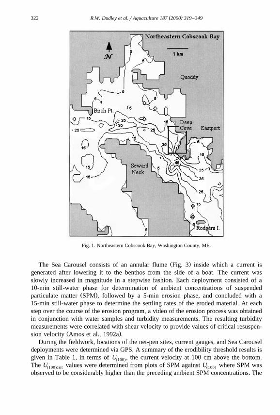
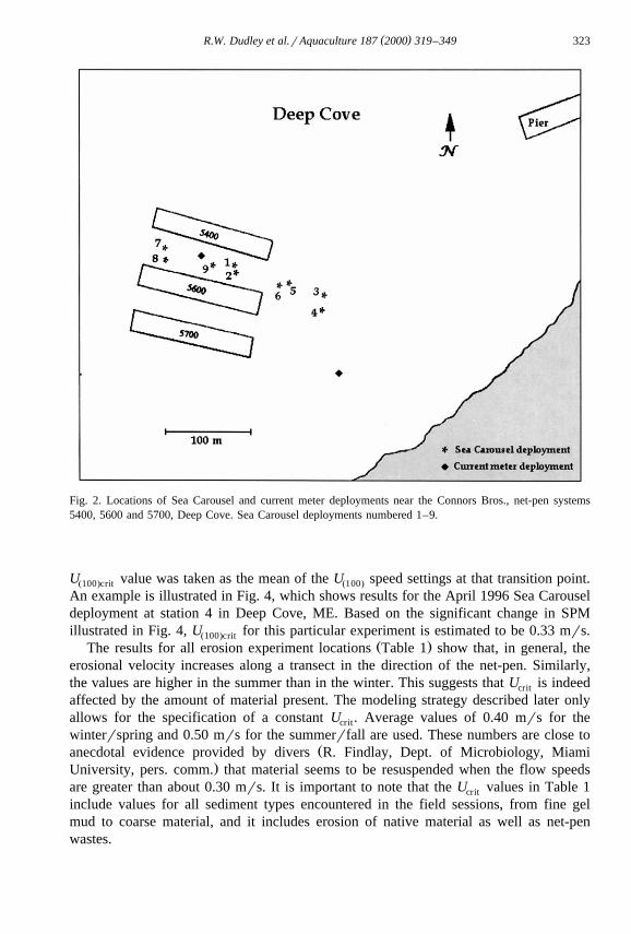
Ž .cial lease site at Deep Cove in Cobscook Bay Fig. 1 near Eastport, ME. This siteŽ .contains three pen-systems Fig. 2 consisting of net-covered cages arranged in rows of

10 cages, with two rows forming an independent floating pen-system, each holdingabout 5000 fish. Since it was possible that the erosion threshold varied with the amountof material already accumulated, the Sea Carousel was deployed at nine locations tomeasure seabed erosion: three near the center of the site, four locations at differentpoints on the sedimentation gradient, and two control locations closer to land deemed tobe unaffected by the net-pen operation. As a consequence of higher feeding rates in thesummer, and more frequent storm-induced erosional events in the winter, there is likelyto be seasonal variation in the amounts of net-pen wastes present. Data were hencecollected at two different times: in April 1996 and in September 1996.


Fig. 1. Northeastern Cobscook Bay, Washington County, ME.

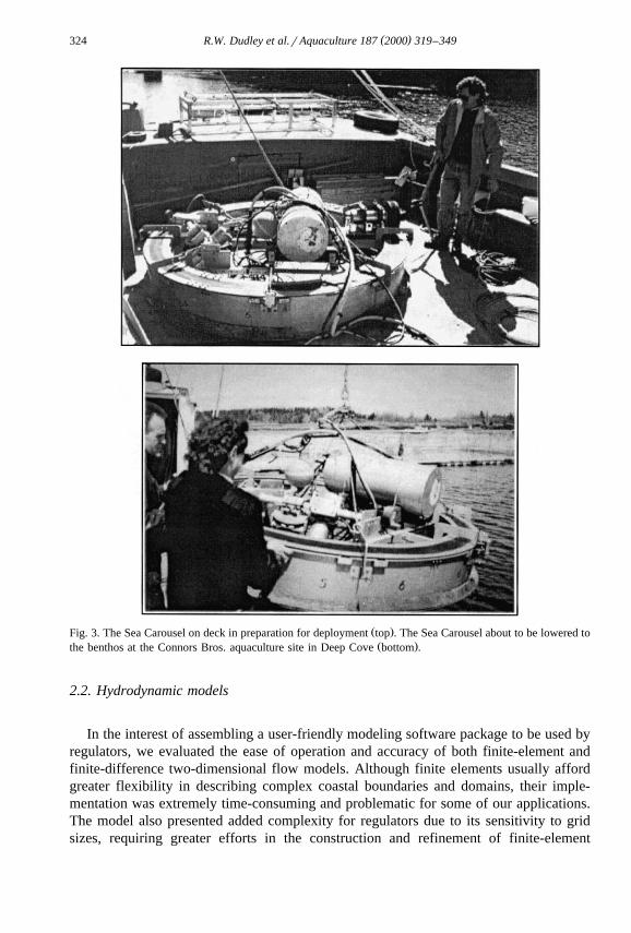
Ž .The Sea Carousel consists of an annular flume Fig. 3 inside which a current isgenerated after lowering it to the benthos from the side of a boat. The current wasslowly increased in magnitude in a stepwise fashion. Each deployment consisted of a10-min still-water phase for determination of ambient concentrations of suspended

Ž .particulate matter SPM , followed by a 5-min erosion phase, and concluded with a15-min still-water phase to determine the settling rates of the eroded material. At eachstep over the course of the erosion program, a video of the erosion process was obtainedin conjunction with water samples and turbidity measurements. The resulting turbiditymeasurements were correlated with shear velocity to provide values of critical resuspen-

Ž .sion velocity Amos et al., 1992a .During the fieldwork, locations of the net-pen sites, current gauges, and Sea Carousel

deployments were determined via GPS. A summary of the erodibility threshold results isgiven in Table 1, in terms of U , the current velocity at 100 cm above the bottom.Ž100.The U values were determined from plots of SPM against U where SPM wasŽ100.crit Ž100.observed to be considerably higher than the preceding ambient SPM concentrations. The


Fig. 2. Locations of Sea Carousel and current meter deployments near the Connors Bros., net-pen systems5400, 5600 and 5700, Deep Cove. Sea Carousel deployments numbered 1–9.

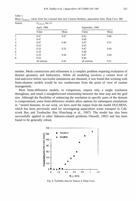
U value was taken as the mean of the U speed settings at that transition point.Ž100.crit Ž100.An example is illustrated in Fig. 4, which shows results for the April 1996 Sea Carouseldeployment at station 4 in Deep Cove, ME. Based on the significant change in SPMillustrated in Fig. 4, U for this particular experiment is estimated to be 0.33 mrs.Ž100.crit

Ž .The results for all erosion experiment locations Table 1 show that, in general, theerosional velocity increases along a transect in the direction of the net-pen. Similarly,the values are higher in the summer than in the winter. This suggests that U is indeedcrit

affected by the amount of material present. The modeling strategy described later onlyallows for the specification of a constant U . Average values of 0.40 mrs for thecrit

winterrspring and 0.50 mrs for the summerrfall are used. These numbers are close toŽanecdotal evidence provided by divers R. Findlay, Dept. of Microbiology, Miami

.University, pers. comm. that material seems to be resuspended when the flow speedsare greater than about 0.30 mrs. It is important to note that the U values in Table 1crit

include values for all sediment types encountered in the field sessions, from fine gelmud to coarse material, and it includes erosion of native material as well as net-penwastes.


Ž .Fig. 3. The Sea Carousel on deck in preparation for deployment top . The Sea Carousel about to be lowered toŽ .the benthos at the Connors Bros. aquaculture site in Deep Cove bottom .

2.2. Hydrodynamic models

In the interest of assembling a user-friendly modeling software package to be used byregulators, we evaluated the ease of operation and accuracy of both finite-element andfinite-difference two-dimensional flow models. Although finite elements usually affordgreater flexibility in describing complex coastal boundaries and domains, their imple-mentation was extremely time-consuming and problematic for some of our applications.The model also presented added complexity for regulators due to its sensitivity to gridsizes, requiring greater efforts in the construction and refinement of finite-element


Table 1Mean U values from Sea Carousel data near Connors Brothers, aquaculture farm, Deep Cove, MEŽ100.crit

Ž .Station U mrsŽ100.crit

April, 1996 September, 1996

Value Mean Value Mean

1 0.47 0.47 0.62 0.662 0.47 0.693 0.47 0.40 0.47 0.514 0.33 0.555 0.33 0.33 0.47 0.446 0.33 0.407 0.33 0.44 0.47 0.448 0.55 0.40

all stations 0.42 all stations 0.51

meshes. Mesh construction and refinement is a complex problem requiring evaluation ofdomain geometry and bathymetry. While all modeling involves a certain level oftrial-and-error before successful simulations are obtained, it was found that working withfinite-element models would be too cumbersome from the point of view of routinemanagement.

Most finite-difference models, in comparison, require only a single resolutionthroughout, and entail a straightforward relationship between the time step and the gridsize. Although the flexibility of enhancing the resolution in specific parts of the domainis compromised, some finite-difference models allow options for subsequent simulationsin ‘‘nested domains. In our work, we have used the output from the model DUCHESS,which has been previously used for investigating aquaculture waste transport in Cob-

Ž .scook Bay and Toothacher Bay Panchang et al., 1997 . The model has also beenŽ .successfully applied to other fisheries-related problems Newell, 1991 and has been

found to be generally robust.

Fig. 4. Turbidity data for Station 4, Deep Cove.


One limitation of DUCHESS and many other finite-difference models is that theylack a convenient graphical user interface to expedite the modeling process by aiding theuser in model construction, and viewing and interpreting model output. For this reason,we made efforts to interface DUCHESS with a software package called Surface-water

Ž .Modeling System SMS developed at the Brigham Young University EngineeringŽ .Computer Graphics Laboratory ECGL in cooperation with the Army Corps of Engi-

Ž .neers Jones and Richards, 1992; ECGL, 1995 . The SMS software provides the userwith various tools and pull-down menus to facilitate digitizing scanned topographymaps, constructing computational meshes, and displaying and animating solution datasets with color contouring and vectors. Although originally intended for finite-elementgrid generation, we developed a utility program called DUCHSMS which indirectlylinks any finite-difference model to the graphical features of SMS. DUCHSMS facili-tates construction of the model domain using SMS, and graphical viewing of the flowmodel output. It enables bathymetry digitized with SMS to be exported in a formrequired by DUCHESS as input and also transforms DUCHESS output into a formreadable by SMS. This allows easy graphical display and animation of flow solutionsobtained from DUCHESS in SMS.

In addition to two-dimensional flow modeling, wave modeling was performed for thedetermination of wave induced velocities. The Automated Coastal Engineering SystemŽ . Ž .ACES United States Army Corps of Engineers, 1992 was incorporated into theAWATS modeling strategy to estimate wave conditions for coastal areas subject tosignificant wind fetch. The model requires, as input, a description of the coastalgeometry in the form of fetch lengths in various compass directions converging on thepoint of interest and the water depth. The model also requires the input of wind speedand direction. Using representative wind speeds and durations to simulate storm events,

Ž . Ž .the resulting wave height H and period T output by ACES can be used with AiryŽ . Žtheory to compute the wave velocity U using the following equation Dean andwave

.Dalrymple, 1984 :

p Hcosh k zqdŽ .Ž .U s cos kxyv t 1Ž . Ž .wave sinh kdŽ .

where d is the total water depth, x and z represent the horizontal and verticalŽ .coordinates of interest zs0 at the surface and zsyd at the bottom , v is the wave

Ž .frequency s2prT , and k is the wave number determined by the wave dispersionŽ 2 Ž ..relationship v sgk tanh kd .

2.3. Transport model

A transport model called TRANS was developed at the University of Maine tosimulate the advection and dispersion of finfish aquaculture wastes. It is included in theAWATS package, and models the mechanisms of settling, advection and resuspension todescribe the physical transport of fish-pen waste materials. To accomplish this, TRANSrequires spatial and temporal flow-field information, bottom topography data, and

Ž .properties describing the net-pen wastes such as resuspension threshold U , settlingcrit


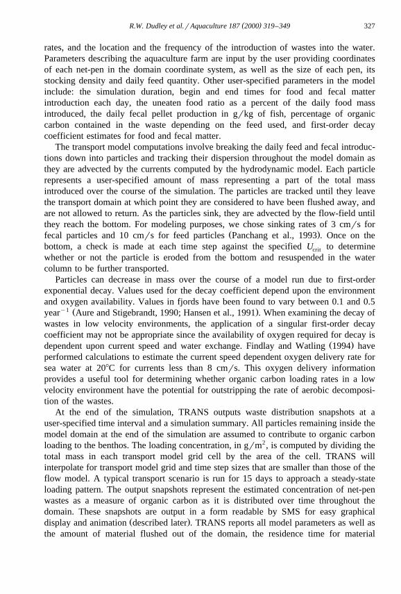
rates, and the location and the frequency of the introduction of wastes into the water.Parameters describing the aquaculture farm are input by the user providing coordinatesof each net-pen in the domain coordinate system, as well as the size of each pen, itsstocking density and daily feed quantity. Other user-specified parameters in the modelinclude: the simulation duration, begin and end times for food and fecal matterintroduction each day, the uneaten food ratio as a percent of the daily food massintroduced, the daily fecal pellet production in grkg of fish, percentage of organiccarbon contained in the waste depending on the feed used, and first-order decaycoefficient estimates for food and fecal matter.

The transport model computations involve breaking the daily feed and fecal introduc-tions down into particles and tracking their dispersion throughout the model domain asthey are advected by the currents computed by the hydrodynamic model. Each particlerepresents a user-specified amount of mass representing a part of the total massintroduced over the course of the simulation. The particles are tracked until they leavethe transport domain at which point they are considered to have been flushed away, andare not allowed to return. As the particles sink, they are advected by the flow-field untilthey reach the bottom. For modeling purposes, we chose sinking rates of 3 cmrs for

Ž .fecal particles and 10 cmrs for feed particles Panchang et al., 1993 . Once on thebottom, a check is made at each time step against the specified U to determinecrit

whether or not the particle is eroded from the bottom and resuspended in the watercolumn to be further transported.

Particles can decrease in mass over the course of a model run due to first-orderexponential decay. Values used for the decay coefficient depend upon the environmentand oxygen availability. Values in fjords have been found to vary between 0.1 and 0.5

y1 Ž .year Aure and Stigebrandt, 1990; Hansen et al., 1991 . When examining the decay ofwastes in low velocity environments, the application of a singular first-order decaycoefficient may not be appropriate since the availability of oxygen required for decay is

Ž .dependent upon current speed and water exchange. Findlay and Watling 1994 haveperformed calculations to estimate the current speed dependent oxygen delivery rate forsea water at 208C for currents less than 8 cmrs. This oxygen delivery informationprovides a useful tool for determining whether organic carbon loading rates in a lowvelocity environment have the potential for outstripping the rate of aerobic decomposi-tion of the wastes.

At the end of the simulation, TRANS outputs waste distribution snapshots at auser-specified time interval and a simulation summary. All particles remaining inside themodel domain at the end of the simulation are assumed to contribute to organic carbonloading to the benthos. The loading concentration, in grm2, is computed by dividing thetotal mass in each transport model grid cell by the area of the cell. TRANS willinterpolate for transport model grid and time step sizes that are smaller than those of theflow model. A typical transport scenario is run for 15 days to approach a steady-stateloading pattern. The output snapshots represent the estimated concentration of net-penwastes as a measure of organic carbon as it is distributed over time throughout thedomain. These snapshots are output in a form readable by SMS for easy graphical

Ž .display and animation described later . TRANS reports all model parameters as well asthe amount of material flushed out of the domain, the residence time for material


introduced on the first day of the simulation, and the maximum load rate and its locationin the model domain in the summary file.

2.4. The AWATS modeling package

We have constructed a package called AWATS that may be suitable for regulatoryuse. This package conveniently links the hydrodynamic and transport models withinformation regarding the net-pen operations and graphically displays results. AWATSincludes the waste transport program TRANS, the graphical interface SMS, and the flow

Žmodel DUCHESS. In the event that the user does not have DUCHESS, output from.another flow model may be used. It also includes a utility program, DUCHSMS, which

Žwas developed to extract flow and bathymetry data for the subdomain of interest i.e. the.general vicinity of the net-pen, specified by the user in the form of a rectangle from the

Ž .output files of the flow model DUCHESS or alternative and use this information to runTRANS. Details regarding practical use of the various components of AWATS are

Ž .described in Dudley et al. 1998 .Executing AWATS produces two forms of output. First, the simulation summary

describes all user-defined parameters and calculated quantities like flushing efficiencyfor particles introduced into the domain, residence time, and the sedimentation rate andlocation of the point with greatest accumulation in the subdomain. The other is a datafile that contains snapshots of the dispersion of net-pen wastes over the simulation,suitable for plotting in SMS for viewingranimation. TRANS uses the model flowsolution to compute the mean and maximum velocity at the location of greatest organic

Ž .carbon loading, and also the tidal prism ratio TPR of the transport domain. The TPRcan provide a first-order estimate of water exchange in the domain due to tidal flushing,which provides more oxygen to aerobic organisms for decomposing organic wastes. Theratio is defined:

TPRs BVHTyBVLT rBVHT 2Ž . Ž .where BVHT and BVLT are the basin volumes at high and low tide, respectively, andthe numerator is known as the tidal prism. Use of the TPR is considered to be areasonable method for comparison of flushing of small harbors that are directly

Žconnected to ambient waters and do not have freshwater inflows Nece and Falconer,. Ž .1989 . Gillibrand and Turrell 1997 use similar flushing parameters as a method to help

evaluate the hydrography of fjordic sea lochs and model the potential impact of fishfarms. Computation of flushing of bays can provide regulators with another factor foridentifying aquaculture sites where organic enrichment is likely to become a problem.

3. Results and discussion

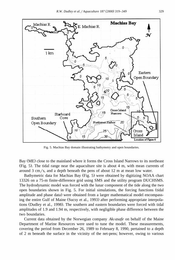
3.1. Simulation of net-pen waste distribution in Machias Bay, ME

Ž .An aquaculture operation run by Atlantic Salmon of Maine ASMI is located inNorthwest Harbor off Cross Island. The island is situated near the mouth of Machias


Fig. 5. Machias Bay domain illustrating bathymetry and open boundaries.

Ž .Bay ME close to the mainland where it forms the Cross Island Narrows to its northeastŽ .Fig. 5 . The tidal range near the aquaculture site is about 4 m, with mean currents ofaround 3 cmrs, and a depth beneath the pens of about 12 m at mean low water.

Ž .Bathymetric data for Machias Bay Fig. 5 were obtained by digitizing NOAA chart13326 on a 75-m finite-difference grid using SMS and the utility program DUCHSMS.The hydrodynamic model was forced with the lunar component of the tide along the two

Žopen boundaries shown in Fig. 5. For initial simulations, the forcing functions tidal.amplitude and phase data were obtained from a larger mathematical model encompass-

Ž .ing the entire Gulf of Maine Sucsy et al., 1993 after performing appropriate interpola-Ž .tions Dudley et al., 1998 . The southern and eastern boundaries were forced with tidal

amplitudes of 1.9 and 1.94 m, respectively, with negligible phase difference between thetwo boundaries.

Current data obtained by the Norwegian company AkÕasafe on behalf of the MaineDepartment of Marine Resources were used to tune the model. These measurements,covering the period from December 26, 1989 to February 8, 1990, pertained to a depthof 2 m beneath the surface in the vicinity of the net-pens; however, owing to various


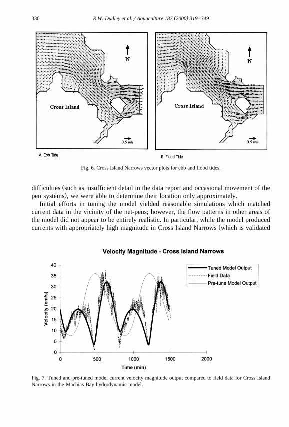
Fig. 6. Cross Island Narrows vector plots for ebb and flood tides.

Ždifficulties such as insufficient detail in the data report and occasional movement of the.pen systems , we were able to determine their location only approximately.

Initial efforts in tuning the model yielded reasonable simulations which matchedcurrent data in the vicinity of the net-pens; however, the flow patterns in other areas ofthe model did not appear to be entirely realistic. In particular, while the model produced

Žcurrents with appropriately high magnitude in Cross Island Narrows which is validated

Fig. 7. Tuned and pre-tuned model current velocity magnitude output compared to field data for Cross IslandNarrows in the Machias Bay hydrodynamic model.


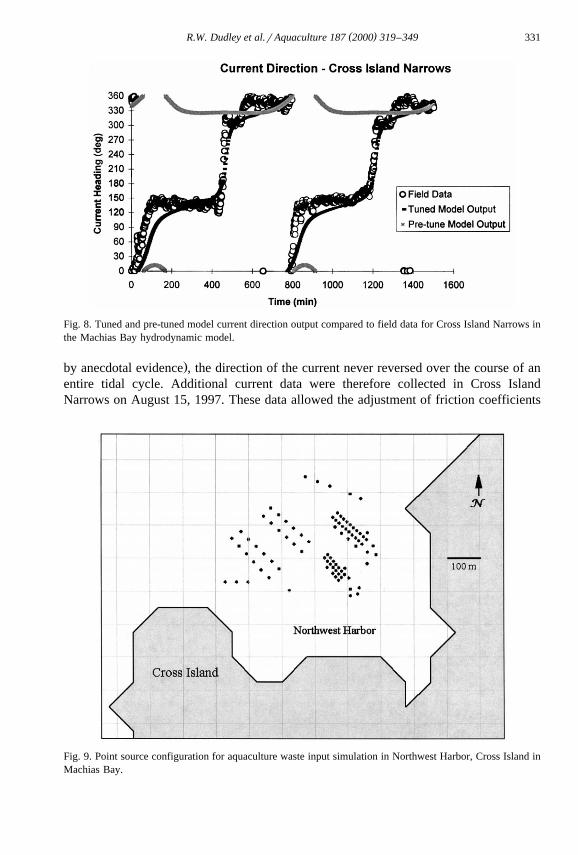
Fig. 8. Tuned and pre-tuned model current direction output compared to field data for Cross Island Narrows inthe Machias Bay hydrodynamic model.

.by anecdotal evidence , the direction of the current never reversed over the course of anentire tidal cycle. Additional current data were therefore collected in Cross IslandNarrows on August 15, 1997. These data allowed the adjustment of friction coefficients

Fig. 9. Point source configuration for aquaculture waste input simulation in Northwest Harbor, Cross Island inMachias Bay.


over various zones, varying from 0.008 to 0.03, as well as improved specification oftidal amplitudes and phases at each open boundary. Model results shown in Fig. 6indicate that the currents in Cross Island Narrows reverse directions over a tidal cycle.Further, Figs. 7 and 8 show modeled velocity magnitudes and directions for a point inCross Island Narrows before and after tuning with the August 15, 1997 data. Thisillustrates the importance of using some field data for producing reliable modelsimulations in the overall domain. At several grid points in the vicinity of theaquaculture net-pens at Cross Island, the model produces currents of 3–5 cmrspredominantly in the east–west direction, which is consistent with the AkÕasafe data.Flow model outputs illustrated in Figs. 6–8 were used as input to the transport model.

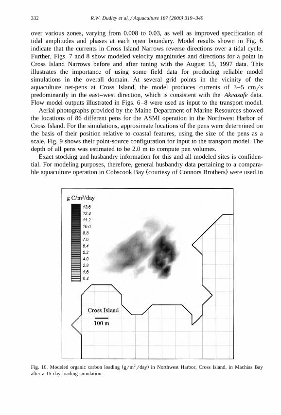
Aerial photographs provided by the Maine Department of Marine Resources showedthe locations of 86 different pens for the ASMI operation in the Northwest Harbor ofCross Island. For the simulations, approximate locations of the pens were determined onthe basis of their position relative to coastal features, using the size of the pens as ascale. Fig. 9 shows their point-source configuration for input to the transport model. Thedepth of all pens was estimated to be 2.0 m to compute pen volumes.

Exact stocking and husbandry information for this and all modeled sites is confiden-tial. For modeling purposes, therefore, general husbandry data pertaining to a compara-

Ž .ble aquaculture operation in Cobscook Bay courtesy of Connors Brothers were used in

Ž 2 .Fig. 10. Modeled organic carbon loading grm rday in Northwest Harbor, Cross Island, in Machias Bayafter a 15-day loading simulation.


Ž .conjunction with data from Laird and Needham 1988 . These data were used toestimate pen stocking density, daily feed quantities per pen and fecal production per unitmass of fish for the each site. Stocking densities can range from 10–50 kgrm3 and daily

Žfeed quantities can range from 0.1–8.0 kgr100 kg fish biomass Laird and Needham,.1988; Beveridge, 1996; Panchang et al., 1997 . For transport modeling purposes for this

study, a stocking density of 20 kgrm3 and daily feed quantity of 1.5 kgr100 kg fishwere used. It is important to note that this nominal aquaculture husbandry informationwas used only for illustrating the application of AWATS. Naturally, regulatory agencieswould have to use specific husbandry information for each site to perform more realistic,site-specific simulations.

Since the model tracks organic carbon as an indicator of waste, the fraction of feedand fecal matter that is organic carbon must be defined. While these fractions can vary,values of 45% and 28% for feed and fecal matter, respectively, were used for modeling

Ž .purposes Findlay and Watling, 1994 . The percentage of feed that goes uneaten andŽ .sinks as waste also varies between 1% and 40%. Findlay and Watling 1994 recom-

mend using a value of 5% or lower for modern Maine aquaculture farms, in particularthose that hand-feed. According to Connors Bros., fecal production is estimated to be1.7–2.1 grkg fish. An intermediate value of 1.9 grkg fish was used for modeling.Sinking rates of fish feed and fecal matter were experimentally determined by Panchang

Ž .et al. 1997 . Settling rates of 50 observations of fecal pellets resulted in a mean settlingrate of 3.2 cmrs with 70% of the observations between 2 and 4 cmrs. Settling rates for

Žfeed and fecal pellets of 10 and 3 cmrs are used in the transport modeling Warren-

Fig. 11. Modeled maximum current velocities for Northwest Harbor, Cross Island.


.Hansen, 1982; Findlay and Watling, 1994; Panchang et al., 1997 . For modelingpurposes, the introduction of waste feed and fecal pellets is assumed to be uniform andto occur 24 h a day. Feed and fecal particles are introduced in the model simultaneouslyevery 2 h from every point-source pen. Though TRANS can accommodate any desired

Ž .particle introduction schedule including a time lag between feed and fecal material , auniform introduction scenario would more closely model a steady-state loading result. Asimulation duration of 15 days was chosen to estimate a steady-state loading pattern,since the daily 0.8 h shift in the lunar tide causes the tides to exactly repeat after thisduration.

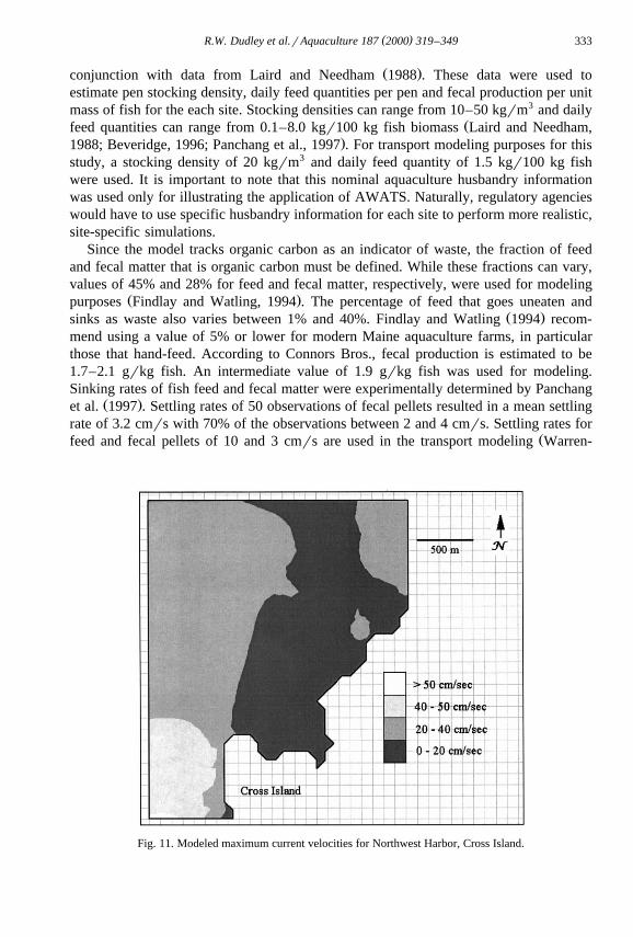
Ž 2 .Fig. 10 shows the modeled loading pattern of organic carbon g Crm rday at theASMI aquaculture site as obtained from AWATS. The results are averaged over a15-day loading simulation. For this simulation, the U value was set at 40 cmrs. Thecrit

eastern and southeastern portions of the aquaculture site receive the highest loadingŽ .receiving a maximum organic carbon loading rate averaged over 15 days of 14.1

grm2rday.Ž .A maximum velocity map obtained from AWATS Fig. 11 shows that modeled tidal

currents in Northwest Harbor never exceed 20 cmrs, suggesting that the ASMI

Fig. 12. Blue Hill Bay tidal model computational domain.


aquaculture operation may be located in a depositional area. The mean and maximumvelocities computed by the model for this particular area are 3.9 and 6.8 cmrs,respectively. Though not high enough to exceed the U criterion for resuspension, thecrit

currents in this area could supply sufficient oxygen to the benthos for adequate rates ofdecay of the effluent as well as high rates of water exchange in the embayment to

Ž .prevent adverse impacts on the macrobenthos Drake and Arias, 1997 . The estimatedtheoretical maximum aerobic oxidation for an environment with a minimum 2-h average

2 Žcurrent velocity of 4 cmrs is nearly 17 grm rday of organic carbon Findlay and.Watling, 1994 , which exceeds the highest loading calculated for Machias Bay in the

previous paragraph.

3.2. Simulation of net-pen waste distribution in Blue Hill Bay, ME

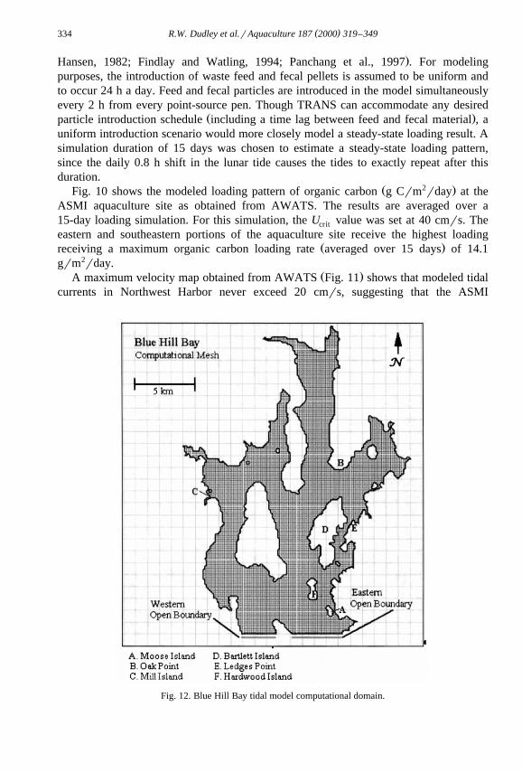
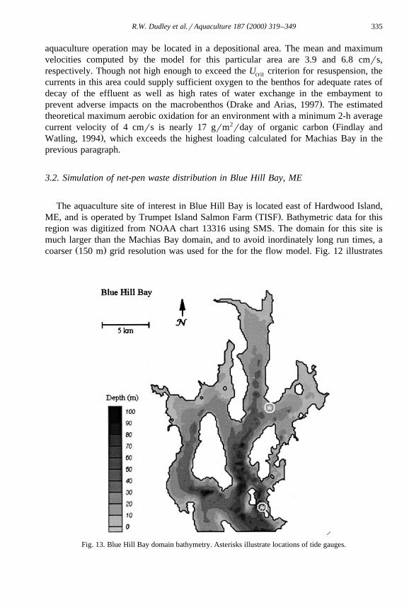
The aquaculture site of interest in Blue Hill Bay is located east of Hardwood Island,Ž .ME, and is operated by Trumpet Island Salmon Farm TISF . Bathymetric data for this

region was digitized from NOAA chart 13316 using SMS. The domain for this site ismuch larger than the Machias Bay domain, and to avoid inordinately long run times, a

Ž .coarser 150 m grid resolution was used for the for the flow model. Fig. 12 illustrates

Fig. 13. Blue Hill Bay domain bathymetry. Asterisks illustrate locations of tide gauges.


Fig. 14. Comparison of current velocity magnitude field data and hydrodynamic model output near HardwoodIsland, Blue Hill Bay.

the Blue Hill Bay domain that was constructed. Tidal amplitude and phase data wereŽ .obtained from the larger Gulf of Maine model data set Sucsy et al., 1993 and the

model was forced by an amplitude of 2.2 m along the southern edge of the domain onŽ .each side of Tinker Island Fig. 12 , with a phase difference of 0.02 radians between the

eastern and western edges of the open boundary.

Fig. 15. Comparison of current direction field data and hydrodynamic model output near Hardwood Island,Blue Hill Bay.


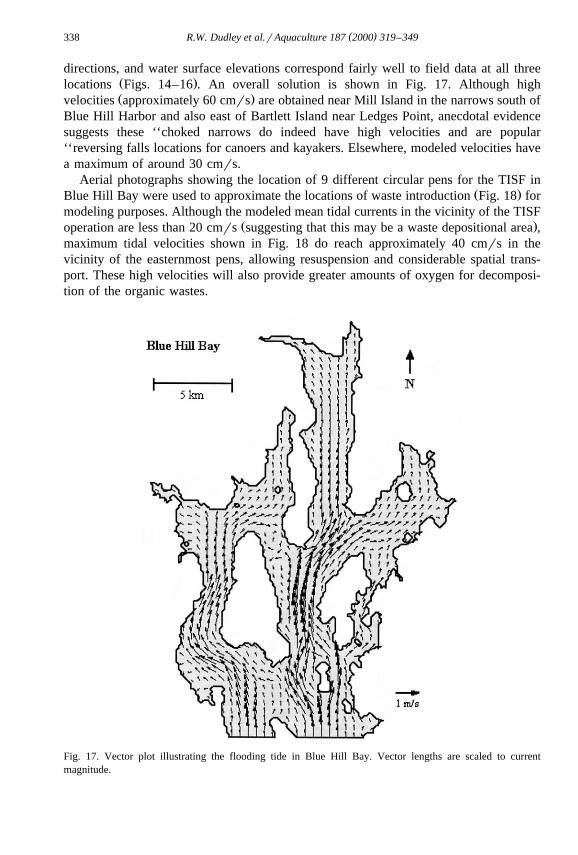
Some trial simulations with various friction specifications led to model failure atabout 11 h into the simulation; investigation revealed that excessively high velocitieswere being produced in the vicinity of Tinker Island. However, each failed simulationprovided a guide to an improved specification of the frictional coefficients, leading to

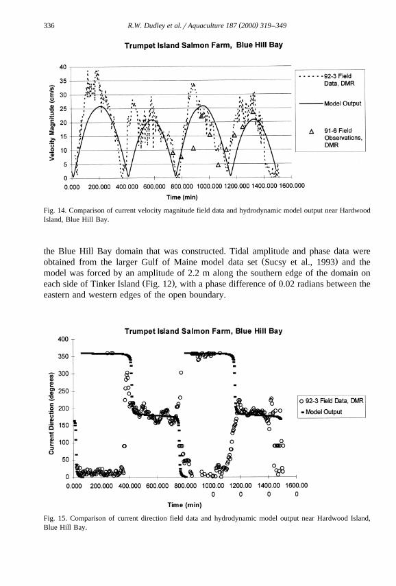
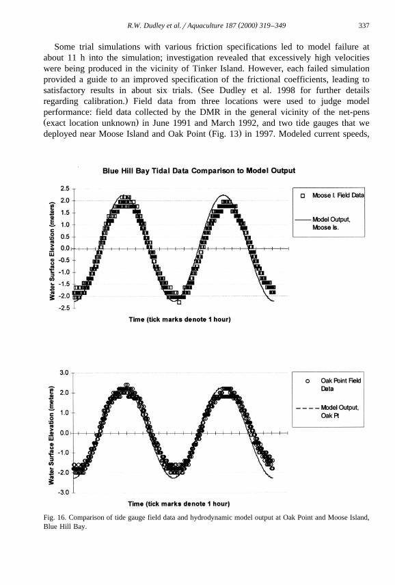
Žsatisfactory results in about six trials. See Dudley et al. 1998 for further details.regarding calibration. Field data from three locations were used to judge model

performance: field data collected by the DMR in the general vicinity of the net-pensŽ .exact location unknown in June 1991 and March 1992, and two tide gauges that we

Ž .deployed near Moose Island and Oak Point Fig. 13 in 1997. Modeled current speeds,

Fig. 16. Comparison of tide gauge field data and hydrodynamic model output at Oak Point and Moose Island,Blue Hill Bay.


directions, and water surface elevations correspond fairly well to field data at all threeŽ .locations Figs. 14–16 . An overall solution is shown in Fig. 17. Although highŽ .velocities approximately 60 cmrs are obtained near Mill Island in the narrows south of

Blue Hill Harbor and also east of Bartlett Island near Ledges Point, anecdotal evidencesuggests these ‘‘choked narrows do indeed have high velocities and are popular‘‘reversing falls locations for canoers and kayakers. Elsewhere, modeled velocities havea maximum of around 30 cmrs.

Aerial photographs showing the location of 9 different circular pens for the TISF inŽ .Blue Hill Bay were used to approximate the locations of waste introduction Fig. 18 for

modeling purposes. Although the modeled mean tidal currents in the vicinity of the TISFŽ .operation are less than 20 cmrs suggesting that this may be a waste depositional area ,

maximum tidal velocities shown in Fig. 18 do reach approximately 40 cmrs in thevicinity of the easternmost pens, allowing resuspension and considerable spatial trans-port. These high velocities will also provide greater amounts of oxygen for decomposi-tion of the organic wastes.

Fig. 17. Vector plot illustrating the flooding tide in Blue Hill Bay. Vector lengths are scaled to currentmagnitude.


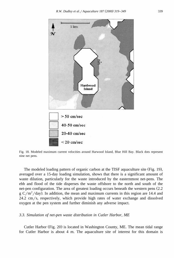
Fig. 18. Modeled maximum current velocities around Harwood Island, Blue Hill Bay. Black dots representnine net pens.

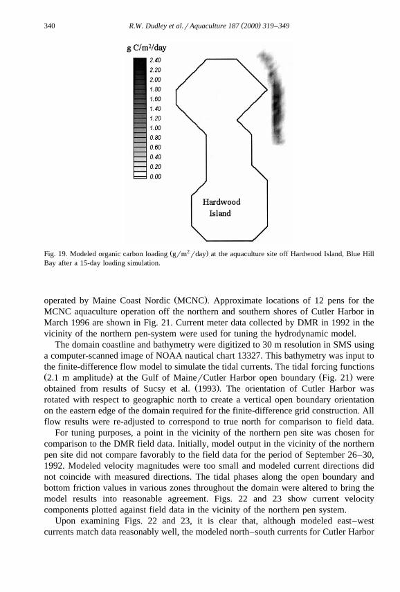
Ž .The modeled loading pattern of organic carbon at the TISF aquaculture site Fig. 19 ,averaged over a 15-day loading simulation, shows that there is a significant amount ofwaste dilution, particularly for the waste introduced by the easternmost net-pens. Theebb and flood of the tide disperses the waste offshore to the north and south of the

Žnet-pen configuration. The area of greatest loading occurs beneath the western pens 2.22 .g Crm rday . In addition, the mean and maximum currents in this region are 14.4 and

24.2 cmrs, respectively, which provide high rates of water exchange and dissolvedoxygen at the pen system and further diminish any adverse impact.

3.3. Simulation of net-pen waste distribution in Cutler Harbor, ME

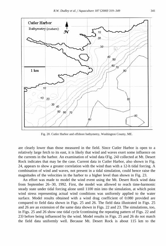
Ž .Cutler Harbor Fig. 20 is located in Washington County, ME. The mean tidal rangefor Cutler Harbor is about 4 m. The aquaculture site of interest for this domain is


Ž 2 .Fig. 19. Modeled organic carbon loading grm rday at the aquaculture site off Hardwood Island, Blue HillBay after a 15-day loading simulation.

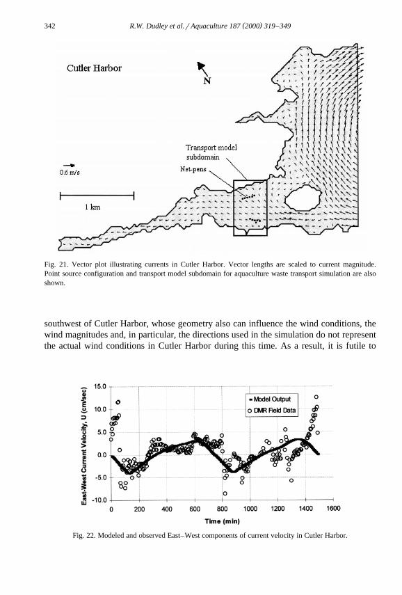
Ž .operated by Maine Coast Nordic MCNC . Approximate locations of 12 pens for theMCNC aquaculture operation off the northern and southern shores of Cutler Harbor inMarch 1996 are shown in Fig. 21. Current meter data collected by DMR in 1992 in thevicinity of the northern pen-system were used for tuning the hydrodynamic model.

The domain coastline and bathymetry were digitized to 30 m resolution in SMS usinga computer-scanned image of NOAA nautical chart 13327. This bathymetry was input tothe finite-difference flow model to simulate the tidal currents. The tidal forcing functionsŽ . Ž .2.1 m amplitude at the Gulf of MainerCutler Harbor open boundary Fig. 21 were

Ž .obtained from results of Sucsy et al. 1993 . The orientation of Cutler Harbor wasrotated with respect to geographic north to create a vertical open boundary orientationon the eastern edge of the domain required for the finite-difference grid construction. Allflow results were re-adjusted to correspond to true north for comparison to field data.

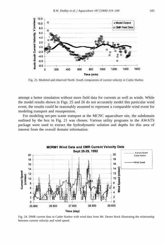
For tuning purposes, a point in the vicinity of the northern pen site was chosen forcomparison to the DMR field data. Initially, model output in the vicinity of the northernpen site did not compare favorably to the field data for the period of September 26–30,1992. Modeled velocity magnitudes were too small and modeled current directions didnot coincide with measured directions. The tidal phases along the open boundary andbottom friction values in various zones throughout the domain were altered to bring themodel results into reasonable agreement. Figs. 22 and 23 show current velocitycomponents plotted against field data in the vicinity of the northern pen system.

Upon examining Figs. 22 and 23, it is clear that, although modeled east–westcurrents match data reasonably well, the modeled north–south currents for Cutler Harbor


Fig. 20. Cutler Harbor and offshore bathymetry, Washington County, ME.

are clearly lower than those measured in the field. Since Cutler Harbor is open to arelatively large fetch to its east, it is likely that wind and waves exert some influence on

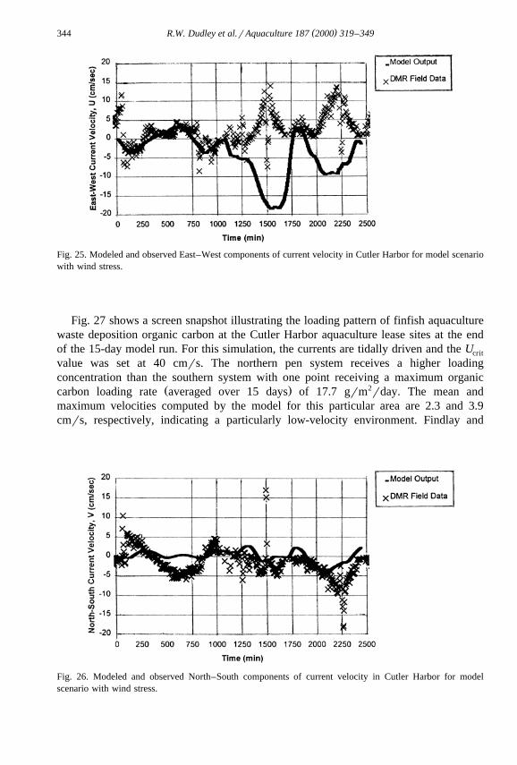
Ž .the currents in the harbor. An examination of wind data Fig. 24 collected at Mt. DesertRock indicates that may be the case. Current data in Cutler Harbor, also shown in Fig.24, appears to show a greater correlation with the wind than with a 12-h tidal forcing. Acombination of wind and waves, not present in a tidal simulation, could hence raise themagnitudes of the velocities in the harbor to a higher level than shown in Fig. 23.

An effort was made to model the wind event using the Mt. Desert Rock wind datafrom September 26–30, 1992. First, the model was allowed to reach time-harmonicsteady state under tidal forcing alone until 1100 min into the simulation, at which pointwind stress representing actual wind conditions was uniformly applied to the watersurface. Model results obtained with a wind drag coefficient of 0.080 provided arecompared to field data shown in Figs. 25 and 26. The field data illustrated in Figs. 25and 26 are an extension of the same data shown in Figs. 22 and 23. The simulations, too,

Žin Figs. 25 and 26 show one tidal cycle continuing the repeating pattern of Figs. 22 and.23 before being influenced by the wind. Model results in Figs. 25 and 26 do not match

the field data uniformly well. Because Mt. Desert Rock is about 115 km to the


Fig. 21. Vector plot illustrating currents in Cutler Harbor. Vector lengths are scaled to current magnitude.Point source configuration and transport model subdomain for aquaculture waste transport simulation are alsoshown.

southwest of Cutler Harbor, whose geometry also can influence the wind conditions, thewind magnitudes and, in particular, the directions used in the simulation do not representthe actual wind conditions in Cutler Harbor during this time. As a result, it is futile to

Fig. 22. Modeled and observed East–West components of current velocity in Cutler Harbor.


Fig. 23. Modeled and observed North–South components of current velocity in Cutler Harbor.

attempt a better simulation without more field data for currents as well as winds. Whilethe model results shown in Figs. 25 and 26 do not accurately model this particular windevent, the results could be reasonably assumed to represent a comparable wind event formodeling transport and resuspension.

For modeling net-pen waste transport at the MCNC aquaculture site, the subdomainoutlined by the box in Fig. 21 was chosen. Various utility programs in the AWATSpackage were used to extract the hydrodynamic solution and depths for this area ofinterest from the overall domain information.

Fig. 24. DMR current data in Cutler Harbor with wind data from Mt. Desert Rock illustrating the relationshipbetween current velocity and wind speed.


Fig. 25. Modeled and observed East–West components of current velocity in Cutler Harbor for model scenariowith wind stress.

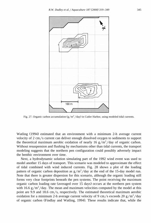
Fig. 27 shows a screen snapshot illustrating the loading pattern of finfish aquaculturewaste deposition organic carbon at the Cutler Harbor aquaculture lease sites at the endof the 15-day model run. For this simulation, the currents are tidally driven and the Ucrit

value was set at 40 cmrs. The northern pen system receives a higher loadingconcentration than the southern system with one point receiving a maximum organic

Ž . 2carbon loading rate averaged over 15 days of 17.7 grm rday. The mean andmaximum velocities computed by the model for this particular area are 2.3 and 3.9cmrs, respectively, indicating a particularly low-velocity environment. Findlay and

Fig. 26. Modeled and observed North–South components of current velocity in Cutler Harbor for modelscenario with wind stress.


Ž 2 .Fig. 27. Organic carbon accumulation grm rday in Cutler Harbor, using modeled tidal currents.

Ž .Watling 1994 estimated that an environment with a minimum 2-h average currentvelocity of 2 cmrs current can deliver enough dissolved oxygen to sediments to supportthe theoretical maximum aerobic oxidation of nearly 16 grm2rday of organic carbon.Without resuspension and flushing by mechanisms other than tidal currents, the transportmodeling suggests that the northern pen configuration could possibly adversely impactthe benthic environment over time.

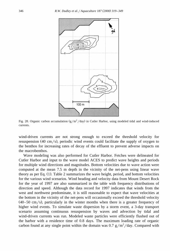
Next, a hydrodynamic solution simulating part of the 1992 wind event was used tomodel another 15 days of transport. This scenario was modeled to approximate the effectof tidal combined with wind induced currents. Fig. 28 shows a plot of the loadingpattern of organic carbon deposition as grm2rday at the end of the 15-day model run.Note that there is greater dispersion for this scenario, although the organic loading stillforms very clear footprints beneath the pen systems. The point receiving the maximum

Ž .organic carbon loading rate averaged over 15 days occurs at the northern pen systemwith 16.6 grm2rday. The mean and maximum velocities computed by the model at thispoint are 9.9 and 18.6 cmrs, respectively. The estimated theoretical maximum aerobicoxidation for a minimum 2-h average current velocity of 9 cmrs exceeds 20 grm2rday

Ž .of organic carbon Findlay and Watling, 1994 . These results indicate that, while the


Ž 2 .Fig. 28. Organic carbon accumulation grm rday in Cutler Harbor, using modeled tidal and wind-inducedcurrents.

wind-driven currents are not strong enough to exceed the threshold velocity forŽ .resuspension 40 cmrs , periodic wind events could facilitate the supply of oxygen to

the benthos for increasing rates of decay of the effluent to prevent adverse impacts onthe macrobenthos.

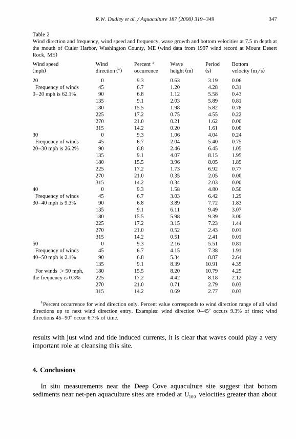
Wave modeling was also performed for Cutler Harbor. Fetches were delineated forCutler Harbor and input to the wave model ACES to predict wave heights and periodsfor multiple wind directions and magnitudes. Bottom velocities due to wave action werecomputed at the mean 7.5 m depth in the vicinity of the net-pens using linear wave

Ž .theory as per Eq. 1 . Table 2 summarizes the wave height, period, and bottom velocitiesfor the various wind scenarios. Wind heading and velocity data from Mount Desert Rockfor the year of 1997 are also summarized in the table with frequency distributions ofdirection and speed. Although the data record for 1997 indicates that winds from thewest and northwest predominate, it is still reasonable to expect that wave velocities atthe bottom in the vicinity of the net-pens will occasionally exceed the threshold velocityŽ .40–50 cmrs , particularly in the winter months when there is a greater frequency ofhigher wind events. To simulate waste dispersion by a storm event, a 3-day transportscenario assuming continuous resuspension by waves and advection by tidal andwind-driven currents was run. Modeled waste particles were efficiently flushed out ofthe harbor with a residence time of 0.8 days. The maximum loading rate of organiccarbon found at any single point within the domain was 0.7 grm2rday. Compared with


Table 2Wind direction and frequency, wind speed and frequency, wave growth and bottom velocities at 7.5 m depth at

Žthe mouth of Cutler Harbor, Washington County, ME wind data from 1997 wind record at Mount Desert.Rock, ME

aWind speed Wind Percent Wave Period BottomŽ . Ž . Ž . Ž . Ž .mph direction 8 occurrence height m s velocity mrs

20 0 9.3 0.63 3.19 0.06Frequency of winds 45 6.7 1.20 4.28 0.31

0–20 mph is 62.1% 90 6.8 1.12 5.58 0.43135 9.1 2.03 5.89 0.81180 15.5 1.98 5.82 0.78225 17.2 0.75 4.55 0.22270 21.0 0.21 1.62 0.00315 14.2 0.20 1.61 0.00


20–30 mph is 26.2% 90 6.8 2.46 6.45 1.05135 9.1 4.07 8.15 1.95180 15.5 3.96 8.05 1.89225 17.2 1.73 6.92 0.77270 21.0 0.35 2.05 0.00315 14.2 0.34 2.03 0.00


30–40 mph is 9.3% 90 6.8 3.89 7.72 1.83135 9.1 6.11 9.49 3.07180 15.5 5.98 9.39 3.00225 17.2 3.15 7.23 1.44270 21.0 0.52 2.43 0.01315 14.2 0.51 2.41 0.01


40–50 mph is 2.1% 90 6.8 5.34 8.87 2.64135 9.1 8.39 10.91 4.35

For winds )50 mph, 180 15.5 8.20 10.79 4.25the frequency is 0.3% 225 17.2 4.42 8.18 2.12

270 21.0 0.71 2.79 0.03315 14.2 0.69 2.77 0.03

a Percent occurrence for wind direction only. Percent value corresponds to wind direction range of all winddirections up to next wind direction entry. Examples: wind direction 0–458 occurs 9.3% of time; winddirections 45–908 occur 6.7% of time.

results with just wind and tide induced currents, it is clear that waves could play a veryimportant role at cleansing this site.

4. Conclusions

In situ measurements near the Deep Cove aquaculture site suggest that bottomsediments near net-pen aquaculture sites are eroded at U velocities greater than about100


40 cmrs in the winter and about 50 cmrs in the summer. These values are used in thedevelopment of the modeling package, AWATS, which can be used for estimating thedispersal of net-pen wastes in a coastal environment with varying currents includingtidal, storm, and wave induced velocities. Application to several aquaculture sites inMaine suggests that AWATS is a convenient tool that can be used to aid with siteevaluation and direction of field monitoring programs. However, the model does notcompletely eliminate the need for field data, which are needed to calibrate the flowmodel and ensure reliability. Rather, it supplements the isolated field measurements andprovides a more complete picture of the flow-field, which is required if resuspension andsubsequent transport is important. Of the three aquaculture sites modeled, the TISFoperation in Blue Hill Bay appears to be in the best location with low accumulationrates, high currents and deep bathymetry for greater dispersion, and high water volumeexchange for waste decay.

The modeling results demonstrate how AWATS can provide not only a picture ofwaste distribution, but information regarding spatial and temporal variations in currentvelocity. Such information could possibly be used in conjunction with benthic oxygendemand data to determine if organic enrichment in high-load regions has the potential toexceed the assimilative capacity of the environment. Adding mechanisms for incorporat-ing oxygen demand of the sediment carbonaceous material to the existing modelingframework will be pursued in future research involving this modeling strategy.

Acknowledgements

Ž .This work was supported in part by the National Marine Fisheries Service NOAAunder the Saltonstall-Kennedy Program and by the University of Maine School ofMarine Sciences. We are grateful to Dr. Carl Amos and Dr. Terri Sutherland of theBedford Institute of Oceanography for performing the fieldwork pertaining to the SeaCarousel and analyzing the erodibility data. We would like to thank Dr. James Manningof NMFS, Mr. John Sowles of the Maine Department of Environmental Protection, Ms.Laurice Churchill and Ms. Tracey Riggens of the Maine Department of MarineResources, and Dr. Stephen Dickson of the Maine Geological Survey for their helpfulassistance and advice over the course of this project. Ms. Riggens provided aerialphotographs and current meter data for the Cutler Harbor site. We thank three anony-mous reviewers whose comments significantly improved this paper.

References

Amos, C.L., Daborn, G.R., Christian, H.A., Atkinson, A., Robertson, A., 1992a. In situ erosion measurementson fine-grained sediments from the Bay of Fundy. Mar. Geol. 108, 175–196.

Amos, C.L., Grant, J., Daborn, G.R., Black, K., 1992b. Sea carousel — a benthic, annular flume. Estuarine,Coastal Shelf Sci. 34, 557–577.

Aure, J., Stigebrandt, A., 1990. Quantitative estimates of the eutrophication effects of fish farming on fjords.Aquaculture 90, 135–156.

Beveridge, M.C.M., 1996. Cage Aquaculture. 2nd edn. Fishing News Books, London, UK, 346 pp.


Booij, N., 1989. User Manual for the program DUCHESS, Delft University computer program for 2Dhorizontal estuary and sea surges. Department of Civil Engineering, Delft University of Technology, Delft,The Netherlands.

Dean, R.G., Dalrymple, R.A., 1984. Water Wave Mechanics for Engineers and Scientists. Prentice-Hall,Englewood Cliffs, NJ.

Drake, P., Arias, A.M., 1997. The effect of aquaculture practices on the benthic macroinvertebrate communityŽ .of a lagoon system in the Bay of Cadiz Southwestern Spain . Estuaries 20, 677–688.

Dudley, R.W., Panchang, V.G., Newell, C.R., 1998. AWATS: a net-pen aquaculture waste transport simulatorŽ .for management purposes. In: Howell, W.H. Ed. , Proc. 26th US–Japan Aquaculture Symposium,

Ž .Durham, New Hampshire, Nov. 1997. US–Japan Cooperative Program in Natural Resources UJNR Tech.Rept. No. 26. pp. 215–228.

ECGL, 1995. SMS Surface Water Modeling System Reference Manual. Brigham Young University Engineer-ing Computer Graphics, Laboratory, Provo, UT.

Findlay, R.H., Watling, L., 1994. Toward a process level model to predict the effects of salmon net-penŽ .aquaculture on the benthos, pp. 47–78. In: Hargrave, B.T. Ed. , Modeling Benthic Impacts of Organic

Enrichment from Marine Aquaculture. Canadian Technical Report of Fisheries and Aquatic Sciences 1949:xiq125 p.

Gillibrand, P.A., Turrell, W.R. et al., 1997. The use of simple models in the regulation of the impact of fishfarms on water quality in Scottish sea lochs. Aquaculture 159, 33–46.

Gowen, R.J., Bradbury, N.B., Brown, J.R., 1989. The use of simple models in assessing two of the interactionsbetween fish-farming and the marine environment. In: DePauw, N., Jaspers, E., Ackerfors, H., Wilkins, N.Ž .Eds. , Aquaculture — A Biotechnology in Progress. European Aquaculture Society, Belgium, pp.1071–1080.

Hansen, P.K., Pittman, K., Ervik, A., 1991. Organic waste from marine fish farms — effects on the sea bed.Ž .In: Makinen, T. Ed. , Marine Aquaculture and Environment. Nord 1992 Vol. 22 Nordic Council of

Ministers, Copenhagen, Denmark, pp. 105–119.Jin, X., Kranenberg, C., 1993. Quasi-3d numerical modeling of shallow-water circulation. J. Hydraul. Eng.

119, 458–472.Jones, N.L., Richards, D.R., 1992. Mesh generation for estuarine flow models. J. Waterway, Port, Coastal,

Ocean Eng., ASCE 118, 599–614.Ž .Laird, L., Needham, T. Eds. , Salmon and Trout Farming. Halsted, New York, NY, 271 pp.

Nece, R.E., Falconer, R.A., 1989. Hydraulic modeling of tidal circulation and flushing in coastal basins. Proc.Ž .Inst. Civ. Eng. 86 Part 1 , 913–935.

Newell, C.R., 1991. Development of a model to seed mussel bottom leases to their carrying capacity. Phase 2report, NSF SBIR, ISI8809760.

Panchang, V.G., Cheng, G., Newell, C., 1993. Application of Mathematical Models in the EnvironmentalRegulation of Aquaculture. Tech. Rpt. NSG-TR-93-1, Maine Sea Grant Program, Orono.

Panchang, V.G., Cheng, G., Newell, C., 1997. Modeling hydrodynamics and aquaculture waste transport inCoastal Maine. Estuaries 20, 14–41.

Schneider, C.R., Fridley, 1993. Aquaculture and the Marine Environment: The Shaping of Public Policy.Working Paper for the Workshop, Marine Biological Laboratory, Woods Hole, MA, August 30–September1, 1993.

Sucsy, P.V., Pearce, B., Panchang, V.G., 1993. Comparison of two- and three-dimensional model simulationof the effect of a tidal barrier on the Gulf of Maine tides. J. Phys. Oceanogr. 23, 1231–1248.

Ž .United States Army Corps of Engineers, 1992. ACES Automated Coastal Engineering System . CoastalEngineering Research Center, Dept. of the Army, Waterways Experiment Station, Corps of Engineers,Vicksburg, MS.

Warren-Hansen, I., 1982. Evaluation of matter discharged from trout farming in Denmark. In: Alabaster, J.S.Ž .Ed. , Report on EIFAC Workshop on Fish-farm Effluents. pp. 57–63.

Application of a comprehensive modeling strategy for the management of net-pen aquaculture waste transport

Documents