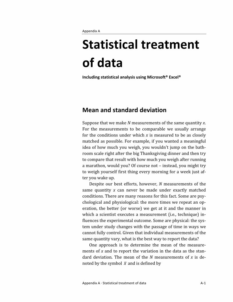
Appendix A Statistical treatment of data A1 Appendix A Statistical treatment of data Including statistical analysis using Microsoft® Excel® Mean and standard deviation Suppose that we make N measurements of the same quantity x. For the measurements to be comparable we usually arrange for the conditions under which x is measured to be as closely matched as possible. For example, if you wanted a meaningful idea of how much you weigh, you wouldn’t jump on the bath room scale right after the big Thanksgiving dinner and then try to compare that result with how much you weigh after running a marathon, would you? Of course not – instead, you might try to weigh yourself first thing every morning for a week just af ter you wake up. Despite our best efforts, however, N measurements of the same quantity x can never be made under exactly matched conditions. There are many reasons for this fact. Some are psy chological and physiological: the more times we repeat an op eration, the better (or worse) we get at it and the manner in which a scientist executes a measurement (i.e., technique) in fluences the experimental outcome. Some are physical: the sys tem under study changes with the passage of time in ways we cannot fully control. Given that individual measurements of the same quantity vary, what is the best way to report the data? One approach is to determine the mean of the measure ments of x and to report the variation in the data as the stan dard deviation. The mean of the N measurements of x is de noted by the symbol x and is defined by

Welcome message from author
This document is posted to help you gain knowledge. Please leave a comment to let me know what you think about it! Share it to your friends and learn new things together.
Transcript
Appendix A ·∙ Statistical treatment of data A-‐1
Appendix A
Statistical treatment of data Including statistical analysis using Microsoft® Excel®
Mean and standard deviation Suppose that we make N measurements of the same quantity x. For the measurements to be comparable we usually arrange for the conditions under which x is measured to be as closely matched as possible. For example, if you wanted a meaningful idea of how much you weigh, you wouldn’t jump on the bath-‐room scale right after the big Thanksgiving dinner and then try to compare that result with how much you weigh after running a marathon, would you? Of course not – instead, you might try to weigh yourself first thing every morning for a week just af-‐ter you wake up. Despite our best efforts, however, N measurements of the same quantity x can never be made under exactly matched conditions. There are many reasons for this fact. Some are psy-‐chological and physiological: the more times we repeat an op-‐eration, the better (or worse) we get at it and the manner in which a scientist executes a measurement (i.e., technique) in-‐fluences the experimental outcome. Some are physical: the sys-‐tem under study changes with the passage of time in ways we cannot fully control. Given that individual measurements of the same quantity vary, what is the best way to report the data? One approach is to determine the mean of the measure-‐ments of x and to report the variation in the data as the stan-‐dard deviation. The mean of the N measurements of x is de-‐noted by the symbol
�
x and is defined by

Appendix A ·∙ Statistical treatment of data A-‐2
�
x =x1 + x2 + x3 ++ xN
N=
xii=1
i=N∑N
where the xi represent the individual measurements of the quantity x and the standard deviation σ is defined by
�
σ =(x1 − x )
2 + (x2− x )2 + (x3− x )
2 ++ (xN − x )2
N=
(xi − x )2
i=1
i=N∑
N
The mean expresses the central tendency in a set of data. The standard deviation expresses the theoretical expectation that 68.27% of the measurements of x will lie within one standard deviation on either side of the mean when x is measured an in-‐finite number of times. Example Table A-‐1 presents the rainfall measured at Boston during Sep-‐tember from 1999 to 2003 and the quantities needed to de-‐termine the mean September rainfall and its standard devia-‐tion. The mean is
Table A-1 September rainfall at Boston, 1999–2003 Quantities needed in the calculation of the mean and of the standard deviation i xi xi –
�
x (xi –
�
x )2 Year Rainfall Deviation from the mean Deviation squared [inch] [inch] [inch2] 1 1999 9.86 5.65 31.92 2 2000 2.87 –1.34 1.80 3 2001 2.29 –1.92 3.69 4 2002 3.39 –0.82 0.67 5 2003 2.65 –1.56 2.43 Sum 21.06 40.51
Appendix A ·∙ Statistical treatment of data A-‐3
�
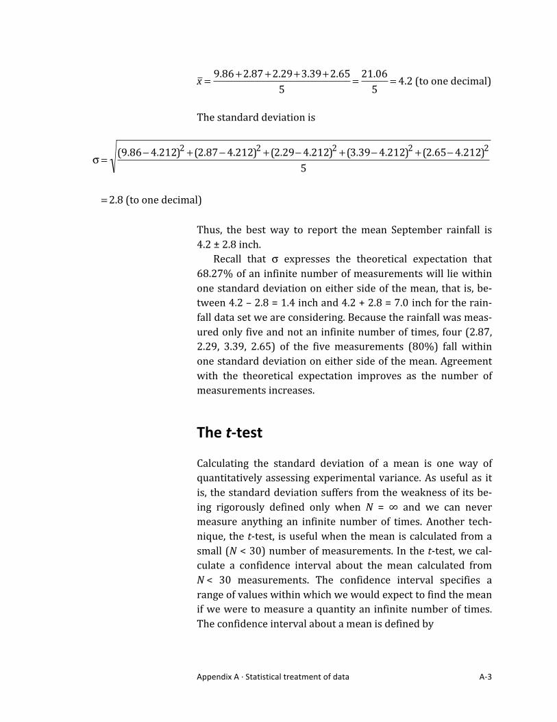
x =9.86+2.87+2.29+3.39+2.65
5=21.065
= 4.2 (to one decimal)
The standard deviation is
�
σ =(9.86−4.212)2 + (2.87−4.212)2 + (2.29−4.212)2 + (3.39−4.212)2 + (2.65−4.212)2
5
=2.8 (to one decimal)
Thus, the best way to report the mean September rainfall is 4.2 ± 2.8 inch. Recall that σ expresses the theoretical expectation that 68.27% of an infinite number of measurements will lie within one standard deviation on either side of the mean, that is, be-‐tween 4.2 – 2.8 = 1.4 inch and 4.2 + 2.8 = 7.0 inch for the rain-‐fall data set we are considering. Because the rainfall was meas-‐ured only five and not an infinite number of times, four (2.87, 2.29, 3.39, 2.65) of the five measurements (80%) fall within one standard deviation on either side of the mean. Agreement with the theoretical expectation improves as the number of measurements increases. The t-‐test Calculating the standard deviation of a mean is one way of quantitatively assessing experimental variance. As useful as it is, the standard deviation suffers from the weakness of its be-‐ing rigorously defined only when N = ∞ and we can never measure anything an infinite number of times. Another tech-‐nique, the t-‐test, is useful when the mean is calculated from a small (N < 30) number of measurements. In the t-‐test, we cal-‐culate a confidence interval about the mean calculated from N < 30 measurements. The confidence interval specifies a range of values within which we would expect to find the mean if we were to measure a quantity an infinite number of times. The confidence interval about a mean is defined by
Appendix A ·∙ Statistical treatment of data A-‐4
�
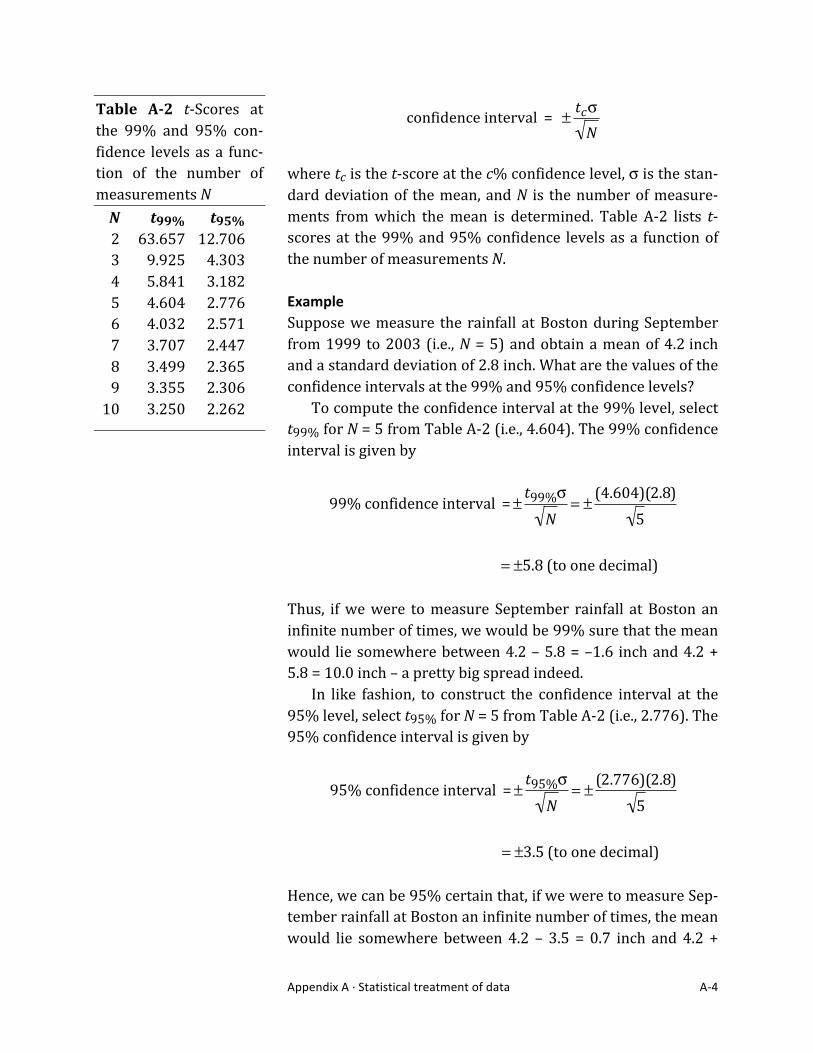
confidence interval = ±tcσ
N
where tc is the t-‐score at the c% confidence level, σ is the stan-‐dard deviation of the mean, and N is the number of measure-‐ments from which the mean is determined. Table A-‐2 lists t-‐scores at the 99% and 95% confidence levels as a function of the number of measurements N. Example Suppose we measure the rainfall at Boston during September from 1999 to 2003 (i.e., N = 5) and obtain a mean of 4.2 inch and a standard deviation of 2.8 inch. What are the values of the confidence intervals at the 99% and 95% confidence levels? To compute the confidence interval at the 99% level, select t99% for N = 5 from Table A-‐2 (i.e., 4.604). The 99% confidence interval is given by
�
99% confidence interval =±t99%σ
N= ±
(4.604)(2.8)5
= ±5.8 (to one decimal)
Thus, if we were to measure September rainfall at Boston an infinite number of times, we would be 99% sure that the mean would lie somewhere between 4.2 – 5.8 = –1.6 inch and 4.2 + 5.8 = 10.0 inch – a pretty big spread indeed. In like fashion, to construct the confidence interval at the 95% level, select t95% for N = 5 from Table A-‐2 (i.e., 2.776). The 95% confidence interval is given by
�
95% confidence interval =±t95%σ
N= ±
(2.776)(2.8)5
= ±3.5 (to one decimal)
Hence, we can be 95% certain that, if we were to measure Sep-‐tember rainfall at Boston an infinite number of times, the mean would lie somewhere between 4.2 – 3.5 = 0.7 inch and 4.2 +
Table A-2 t-‐Scores at the 99% and 95% con-‐fidence levels as a func-‐tion of the number of measurements N N t99% t95% 2 63.657 12.706 3 9.925 4.303 4 5.841 3.182 5 4.604 2.776 6 4.032 2.571 7 3.707 2.447 8 3.499 2.365 9 3.355 2.306 10 3.250 2.262
Appendix A ·∙ Statistical treatment of data A-‐5
3.5 = 7.7 inch. Note that the confidence interval shrinks (from ±5.8 inch at 99% confidence to ±3.5 inch at 95% confidence) if we are willing to hazard a lesser degree of certainty. Incidentally, more than a century of record keeping has shown that the average September rainfall at Boston is 3.47 inch – a value that lies within both the 99% and the 95% confidence intervals. Linear least-‐squares Suppose a data set relating two variables x and y is expected to obey the linear relationship
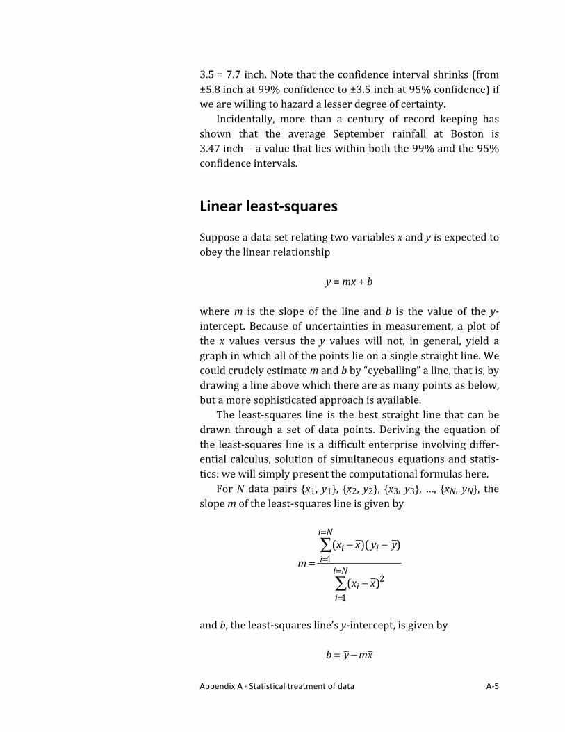
y = mx + b where m is the slope of the line and b is the value of the y-‐intercept. Because of uncertainties in measurement, a plot of the x values versus the y values will not, in general, yield a graph in which all of the points lie on a single straight line. We could crudely estimate m and b by “eyeballing” a line, that is, by drawing a line above which there are as many points as below, but a more sophisticated approach is available. The least-‐squares line is the best straight line that can be drawn through a set of data points. Deriving the equation of the least-‐squares line is a difficult enterprise involving differ-‐ential calculus, solution of simultaneous equations and statis-‐tics: we will simply present the computational formulas here. For N data pairs {x1, y1}, {x2, y2}, {x3, y3}, …, {xN, yN}, the slope m of the least-‐squares line is given by
�
m =
(xi − x )( yi − y )i=1
i=N
∑
(xi − x )2
i=1
i=N
∑
and b, the least-‐squares line’s y-‐intercept, is given by
�
b = y −mx

Appendix A ·∙ Statistical treatment of data A-‐6
where
�
x is the mean of the xi and
�
y is the mean of the yi. The least-‐squares slope itself is subject to uncertainty. One way to express the variation in the data is to report the stan-‐dard error of estimate σm in the least-‐squares slope:
�
σm =
( yi − y )2
i=1
i=N
∑
(xi − x )2
i=1
i=N
∑
⎛
⎝
⎜ ⎜ ⎜ ⎜ ⎜
⎞
⎠
⎟ ⎟ ⎟ ⎟ ⎟
−m2
N −2
where
�
x is the mean of the xi,
�
y is the mean of the yi, m is the least-‐squares slope and N is the number of data pairs used in constructing the least-‐squares line. The standard error of esti-‐mate σm indicates that, because of uncertainties in measure-‐ment, the least-‐squares slope m could be as high as m + σm or as low as m – σm. Example Just in case you don’t hit the lottery, it might be interesting to investigate whether there is a relationship between income
Table A-3 Years of school attended (x) and average household income (y) in thousands of dollars (k$); Calculation of the linear least-‐squares slope m and intercept b i xi yi xi –
�
x yi –
�
y (xi –
�
x )(yi –
�
y ) (xi –
�
x )2 [year] [k$] [year] [k$] [year·k$] [year2] 1 11 32 –3 –30 90 9 2 12 46 –2 –16 32 4 3 13 57 –1 –5 5 1 4 14 60 0 –2 0 0 5 16 83 2 21 42 4 6 18 94 4 32 128 16 Sum 84 372 297 34 Mean 14 62
Appendix A ·∙ Statistical treatment of data A-‐7
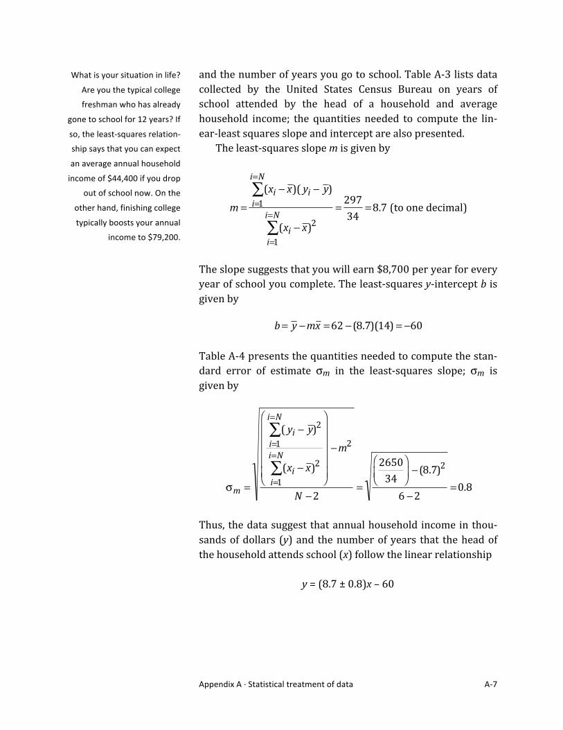
and the number of years you go to school. Table A-‐3 lists data collected by the United States Census Bureau on years of school attended by the head of a household and average household income; the quantities needed to compute the lin-‐ear-‐least squares slope and intercept are also presented. The least-‐squares slope m is given by
�
m =
(xi − x )( yi − y )i=1
i=N
∑
(xi − x )2
i=1
i=N
∑=29734
=8.7 (to one decimal)
The slope suggests that you will earn $8,700 per year for every year of school you complete. The least-‐squares y-‐intercept b is given by
�
b= y −mx =62 − (8.7)(14) = −60 Table A-‐4 presents the quantities needed to compute the stan-‐dard error of estimate σm in the least-‐squares slope; σm is given by
�
σm =
( yi − y )2
i=1
i=N
∑
(xi − x )2
i=1
i=N
∑
⎛
⎝
⎜ ⎜ ⎜ ⎜ ⎜
⎞
⎠
⎟ ⎟ ⎟ ⎟ ⎟
−m2
N −2=
265034
⎛
⎝ ⎜ ⎞
⎠ ⎟ − (8.7)2
6 −2=0.8
Thus, the data suggest that annual household income in thou-‐sands of dollars (y) and the number of years that the head of the household attends school (x) follow the linear relationship
y = (8.7 ± 0.8)x – 60
What is your situation in life?
Are you the typical college
freshman who has already
gone to school for 12 years? If
so, the least-‐squares relation-‐
ship says that you can expect
an average annual household
income of $44,400 if you drop
out of school now. On the
other hand, finishing college
typically boosts your annual
income to $79,200.
Appendix A ·∙ Statistical treatment of data A-‐8
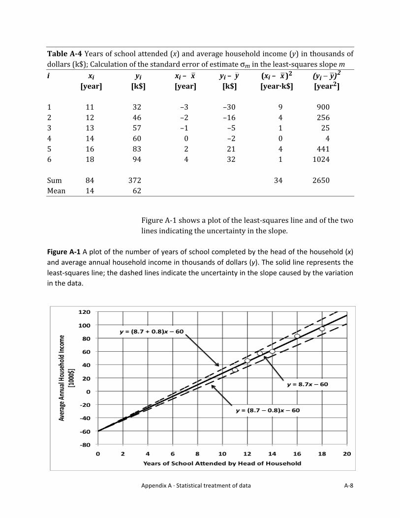
Figure A-‐1 shows a plot of the least-‐squares line and of the two lines indicating the uncertainty in the slope.
Figure A-‐1 A plot of the number of years of school completed by the head of the household (x) and average annual household income in thousands of dollars (y). The solid line represents the least-‐squares line; the dashed lines indicate the uncertainty in the slope caused by the variation in the data.
Table A-4 Years of school attended (x) and average household income (y) in thousands of dollars (k$); Calculation of the standard error of estimate σm in the least-‐squares slope m i xi yi xi – yi –
�
y (xi – )2
�
(yi − y )2
[year] [k$] [year] [k$] [year·k$] [year2] 1 11 32 –3 –30 9 900 2 12 46 –2 –16 4 256 3 13 57 –1 –5 1 25 4 14 60 0 –2 0 4 5 16 83 2 21 4 441 6 18 94 4 32 1 1024 Sum 84 372 34 2650 Mean 14 62
!!
"! !!
"!
Appendix A ·∙ Statistical treatment of data A-‐9
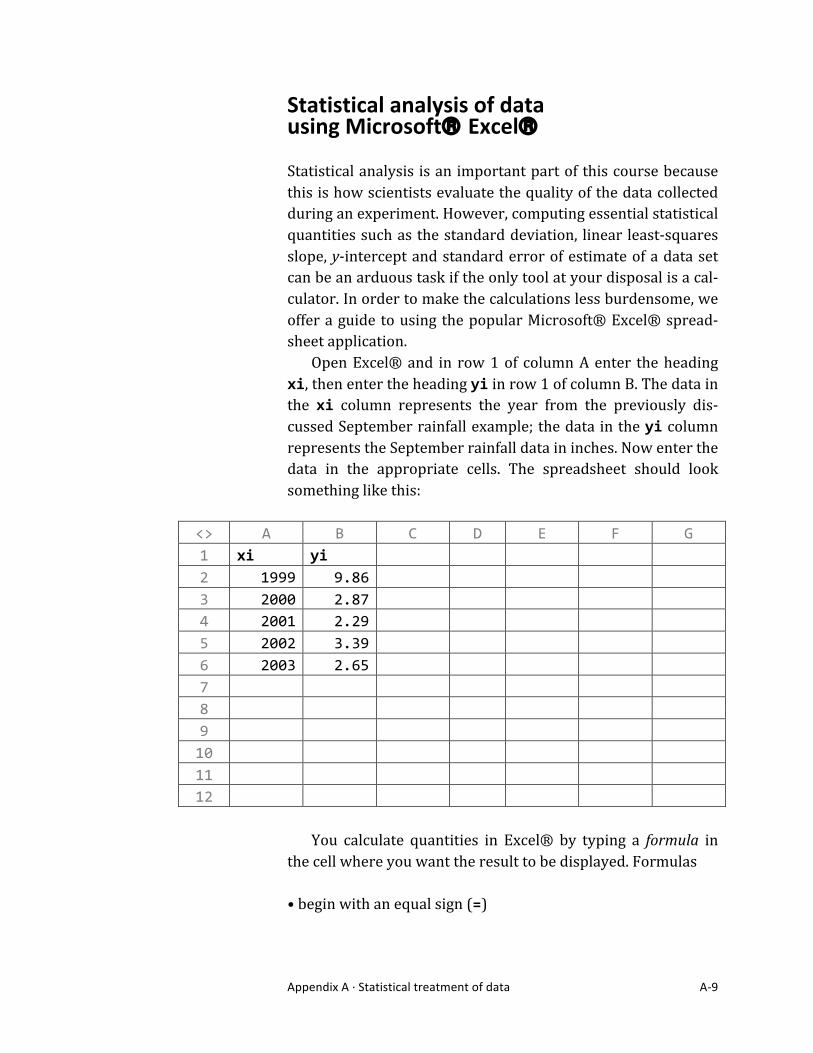
Statistical analysis of data using Microsoft® Excel® Statistical analysis is an important part of this course because this is how scientists evaluate the quality of the data collected during an experiment. However, computing essential statistical quantities such as the standard deviation, linear least-‐squares slope, y-‐intercept and standard error of estimate of a data set can be an arduous task if the only tool at your disposal is a cal-‐culator. In order to make the calculations less burdensome, we offer a guide to using the popular Microsoft® Excel® spread-‐sheet application. Open Excel® and in row 1 of column A enter the heading xi, then enter the heading yi in row 1 of column B. The data in the xi column represents the year from the previously dis-‐cussed September rainfall example; the data in the yi column represents the September rainfall data in inches. Now enter the data in the appropriate cells. The spreadsheet should look something like this:
<> A B C D E F G 1 xi yi 2 1999 9.86 3 2000 2.87 4 2001 2.29 5 2002 3.39 6 2003 2.65 7 8 9 10 11 12
You calculate quantities in Excel® by typing a formula in the cell where you want the result to be displayed. Formulas • begin with an equal sign (=)
Appendix A ·∙ Statistical treatment of data A-‐10
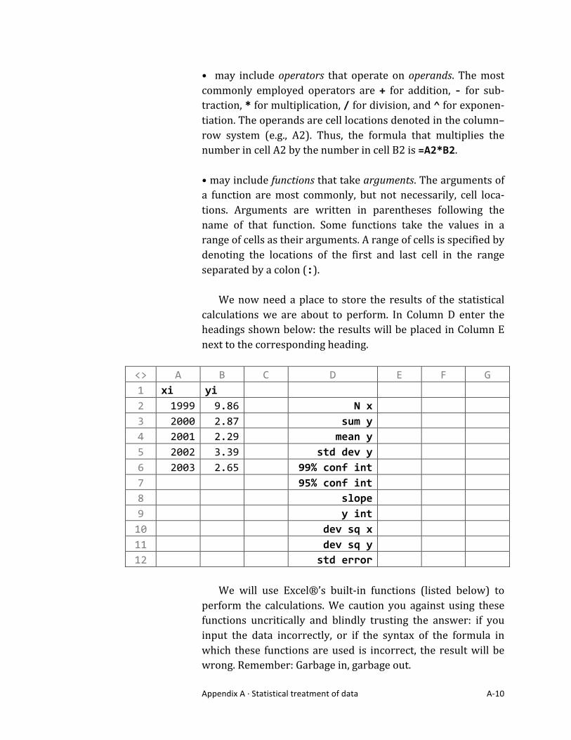
• may include operators that operate on operands. The most commonly employed operators are + for addition, -‐ for sub-‐traction, * for multiplication, / for division, and ^ for exponen-‐tiation. The operands are cell locations denoted in the column–row system (e.g., A2). Thus, the formula that multiplies the number in cell A2 by the number in cell B2 is =A2*B2. • may include functions that take arguments. The arguments of a function are most commonly, but not necessarily, cell loca-‐tions. Arguments are written in parentheses following the name of that function. Some functions take the values in a range of cells as their arguments. A range of cells is specified by denoting the locations of the first and last cell in the range separated by a colon (:). We now need a place to store the results of the statistical calculations we are about to perform. In Column D enter the headings shown below: the results will be placed in Column E next to the corresponding heading.
<> A B C D E F G 1 xi yi 2 1999 9.86 N x 3 2000 2.87 sum y 4 2001 2.29 mean y 5 2002 3.39 std dev y 6 2003 2.65 99% conf int 7 95% conf int 8 slope 9 y int 10 dev sq x 11 dev sq y 12 std error
We will use Excel®’s built-‐in functions (listed below) to perform the calculations. We caution you against using these functions uncritically and blindly trusting the answer: if you input the data incorrectly, or if the syntax of the formula in which these functions are used is incorrect, the result will be wrong. Remember: Garbage in, garbage out.

Appendix A ·∙ Statistical treatment of data A-‐11
COUNT(range) This function counts the number of cells that contain numbers in the specified range; thus, the COUNT() function can be used to calculate the number of measurements N in a data set. Sup-‐pose we wish to find the number of x values in the spreadsheet. The x value data starts at cell A2 and ends at cell A6: entering the formula =COUNT(A2:A6) in cell E2 returns N = 5. SUM(range) This function sums the numbers in the specified range. Sup-‐pose we wish to find the sum of the y values in the spreadsheet (i.e., ∑y). The y value data starts at cell B2 and ends at cell B6: entering the formula =SUM(B2:B6) in cell E3 returns ∑y = 21.06. AVERAGE(range) This function calculates the mean of the numbers in the speci-‐fied range. Suppose we wish to find the mean of the y values in the spreadsheet (i.e.,
�
y ). The y value data starts at cell B2 and ends at cell B6: entering the formula =AVERAGE(B2:B6) in cell E4 returns
�
y = 4.212. STDEVP(range) This function calculates the standard deviation σ of the num-‐bers in the specified range. Suppose we wish to find the stan-‐dard deviation of the y values in the spreadsheet. The y value data starts at cell B2 and ends at cell B6: entering the formula =STDEVP(B2:B6) in cell E5 returns σ = 2.8464181. TINV(probability,degrees of freedom) Excel® lacks a built-‐in function for calculating a confidence in-‐terval when the number of measurements N < 30: the required formula must be constructed by the user. Recall that the confi-‐dence interval about a mean is defined by
�
confidence interval= ±tcσ
N
Appendix A ·∙ Statistical treatment of data A-‐12
where tc is the t-‐score at the c% confidence level, σ is the stan-‐dard deviation of the mean, and N is the number of measure-‐ments from which the mean is determined. Excel® employs the TINV(probability,degrees of freedom) function to determine the appropriate t-‐score. The probability argu-‐ment of the TINV() function corresponds to the confidence level and the degrees of freedom argument of the TINV() function corresponds to the number of measurements, but the correspondences makes sense only to a statistician. If you are calculating a 99% confidence interval, the probability argument of the TINV() function is 0.01. If you are calculating a 95% confidence interval, the probability argument of the TINV() function is 0.05. If you are calculating a 90% confidence interval, the probability argument of the TINV() function is 0.10, and so on. The degrees of freedom argument of the TINV() func-‐tion equals the number of measurements N – 1. If the number of measurements N = 3, the degrees of freedom argument of the TINV() function is 2. If the number of measurements N = 4, the degrees of freedom argument of the TINV() function is 3. If the number of measurements N = 5, the degrees of freedom argument of the TINV() function is 4, and so on. Because N = 5 in the spreadsheet we are considering, the t-‐score at the 99% confidence level is given by TINV(0.01,4) whereas the t-‐score at the 95% confidence level is given by TINV(0.05,4). Suppose we wish to find the 99% confidence interval of the five y values in cells B2 to B6 in the spreadsheet. There are several ways to proceed. The easiest method is first to calcu-‐late the standard deviation σ and to store the result in a cell. Let’s say you enter the formula =STDEVP(B2:B6) in cell E5. Entering the formula =TINV(0.01,4)*E5/SQRT(5) in cell E6 returns the 99% confidence interval = 5.860814209. The for-‐mula =TINV(0.01,4)*STDEVP(B2:B6)/SQRT(5) gives the same result. If you are an Excel® animal, try
=TINV(0.01,COUNT(B2:B6)-‐1)*STDEVP(B2:B6)/SQRT(COUNT(B2:B6))
Suppose we wish to find the 95% confidence interval of the five y values in cells B2 to B6 in the spreadsheet. We can first
Appendix A ·∙ Statistical treatment of data A-‐13
calculate the standard deviation σ: enter the formula =STDEVP(B2:B6) in cell E5. Entering the formula =TINV(0.05,4)*E5/SQRT(5) in cell E7 returns the 95% con-‐fidence interval = 3.534294878, as does entering the formula =TINV(0.05,4)*STDEVP(B2:B6)/SQRT(5), as does entering the formula
=TINV(0.05,COUNT(B2:B6)-‐1)*STDEVP(B2:B6)/SQRT(COUNT(B2:B6))
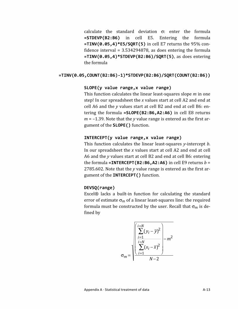
SLOPE(y value range,x value range) This function calculates the linear least-‐squares slope m in one step! In our spreadsheet the x values start at cell A2 and end at cell A6 and the y values start at cell B2 and end at cell B6: en-‐tering the formula =SLOPE(B2:B6,A2:A6) in cell E8 returns m = –1.39. Note that the y value range is entered as the first ar-‐gument of the SLOPE() function. INTERCEPT(y value range,x value range) This function calculates the linear least-‐squares y-‐intercept b. In our spreadsheet the x values start at cell A2 and end at cell A6 and the y values start at cell B2 and end at cell B6: entering the formula =INTERCEPT(B2:B6,A2:A6) in cell E9 returns b = 2785.602. Note that the y value range is entered as the first ar-‐gument of the INTERCEPT() function. DEVSQ(range) Excel® lacks a built-‐in function for calculating the standard error of estimate σm of a linear least-‐squares line: the required formula must be constructed by the user. Recall that σm is de-‐fined by
�
σm =
( yi − y )2
i=1
i=N∑
(xi − x )2
i=1
i=N∑
⎛
⎝
⎜ ⎜ ⎜ ⎜ ⎜
⎞
⎠
⎟ ⎟ ⎟ ⎟ ⎟
−m2
N−2
Appendix A ·∙ Statistical treatment of data A-‐14
where
�
x is the mean of the xi,
�
y is the mean of the yi, m is the least-‐squares slope and N is the number of data pairs used in constructing the least-‐squares line. The function DEVSQ() calculates the quantities
�
Σ(xi − x )2
and
�
Σ( yi − y )2 required in the calculation of σm. In our spread-‐
sheet the x values start at cell A2 and end at cell A6 and the y values start at cell B2 and end at cell B6: entering the formula =DEVSQ(A2:A6) in cell E10 returns the quantity
�
Σ(xi − x )2 =
10. Likewise, entering the formula =DEVSQ(B2:B6) in cell E11 returns the quantity
�
Σ( yi − y )2 = 40.51048.
Let’s suppose that we already calculated the linear least-‐squares slope m of the N = 5 data pairs and placed the result in cell E8. We just placed the value of
�
Σ(xi − x )2 in cell E10 and
the value of
�
Σ( yi − y )2 in cell E11. The value of σm is deter-‐
mined by entering the formula =SQRT(((E11/E10)-‐E8^2)/3) in E12; the value returned is σm = 0.840426082. Note that we have made liberal use of parentheses in constructing the for-‐mula for σm so that Excel® doesn’t get confused about what it’s multiplying, squaring, dividing, and what’s supposed to be the argument of the SQRT() function. You must be very careful about using parentheses when entering Excel® formulas: faulty grouping may return a result, but that result will be wrong.
Related Documents