APPENDIX O KEMPER COUNTY IGCC PROJECT GROUND WATER WITHDRAWAL IMPACT ASSESSMENT

Welcome message from author
This document is posted to help you gain knowledge. Please leave a comment to let me know what you think about it! Share it to your friends and learn new things together.
Transcript
APPENDIX O
KEMPER COUNTY IGCC PROJECT GROUND WATER WITHDRAWAL IMPACT ASSESSMENT

This page intentionally left blank.
KEMPER COUNTY IGCC PROJECT
DESCRIPTION OF THE GROUND WATER FLOW MODEL SIMULATIONS
Prepared by:
115A West Main Street
Benton Harbor, Michigan 49022
ECT No. 080295-0700
June 2009
1 Y:\GDP-09\SOCO\KEMPER\GWRES.DOC—062609
KEMPER COUNTY IGCC PROJECT DESCRIPTION OF THE GROUND WATER FLOW MODEL SIMULATIONS
Mississippi Power Company (Mississippi Power) plans to obtain water for use at the
Kemper County Integrated Gasification Combined-Cycle (IGCC) Project power plant
primarily from two Meridian, Mississippi, publicly owned treatment works (POTWs). Up
to 1 million gallons per day (MGD) of ground water withdrawn from deep onsite wells
might also be used on an as-needed basis. As an alternative, the use of ground water to
fully supply the water requirements for the proposed IGCC facility was also considered.
Ground water flow modeling was performed by Environmental Consulting & Technolo-
gy, Inc. (ECT), to facilitate evaluation of potential impacts from the withdrawal of
1 MGD of ground water from the Massive Sand aquifer for a backup well field. Two
wells withdrawing at a rate of 0.5 MGD each were simulated in cells R182 C92 and
R183 C92 of the model. An alternative simulation, in which cooling water was obtained
from a primary well field withdrawing ground water at a rate of 6.5 MGD, was also com-
pleted. In this alternative case, two wells withdrawing at a rate of 3.25 MGD each were
simulated in cells R182 C92 and R183 C92 of the model.
The quasi three-dimensional Modular Three-Dimensional Finite Difference Ground Wa-
ter Flow Model (MODFLOW) developed at the U.S. Geological Survey (USGS) by
McDonald and Harbaugh (1988, 1996) was applied for this ground water modeling as
presented herein. Ground Water Vistas, a pre- and postprocessing MODFLOW graphical
design interface, was used to complete this modeling effort.
MODEL AREA
The ground water flow model was based on a 34,960-square-mile (mi2) area in northeas-
tern Mississippi modeled by Eric W. Strom of USGS as described in the USGS Water
Resources Investigations Report 98-4171 (i.e., the Strom Model). The model includes the
extent of aquifers in the Cretaceous- and Paleozoic-age sediments that are used as a
source of fresh water. The Strom Model is within the Gulf Coastal Plain physiographic
province on the eastern flank of the Mississippi embayment. The main surface water

2 Y:\GDP-09\SOCO\KEMPER\GWRES.DOC—062609
drainage affecting the ground water flow in the area aquifers are the Tombigbee and
Black Warrior Rivers along the northeastern edge of the model (Strom, 1998).
HYDROGEOLOGY
The hydrogeology of the site area was conceptualized as a three-dimensional, six-layered
system consisting of eight aquifers. The eight aquifers, from youngest to oldest, are the
Coffee Sand, Eutaw-McShan, Gordo, Coker, Massive Sand, Lower Cretaceous, Paleozoic
Iowa, and Devonian. The Coffee Sand, Eutaw-McShan, and Gordo aquifers are
represented in the model by Layers 1, 2 and 3, respectively. The Coker and Iowa aquifers
are jointly represented by Layer 4. The Massive Sand and Devonian are both represented
by Layer 5 since their lateral boundaries do not coincide. Layer 6 represents the lower
Cretaceous. Strom’s Figure 18 (Strom, 1998) depicts a map illustrating the areal extent
and overlap of the fresh water aquifers in the modeled area. (Referenced copies of the
Strom Model report figures are presented in Appendix A of this report.)
Geologic and hydrogeologic data used by Strom to create the model was obtained from
more than 600 borehole geophysical logs and drillers’ logs combined with other pub-
lished stratigraphic information (Strom, 1998). Hydraulic data in the Strom Model was
based on the analyses of borehole geophysical and lithologic logs of water wells, test
holes, and aquifer tests. Figure 1 depicts a generalized hydrogeologic cross-section repre-
sentative of the model area. The sediments include gravel, sand, clay, chalk, and marl of
fluvial-deltaic, continental, and marine shelf origins. Cretaceous sediments generally dip
toward the axis of the Mississippi embayment at the rate of 40 feet per mile (ft/mi), while
the Paleozoic sediments dip toward the south-southwest at rates ranging from 25 to
50 ft/mi. The thickness of these sediments also tends to increase in the down dip direc-
tions (ibid.).
COFFEE SAND AQUIFER—LAYER 1
The Coffee Sand aquifer outcrops in northeastern Mississippi and eastern Tennessee
(Figure 6, Strom, 1998) and is composed of fine- to medium-grained, calcareous to glau-
conitic sand with lenses of silty sand and clay. Well logs indicate that the Coffee Sand

Y:\GDP-09\SOCO\KEMPER\EIS\GWRES-FGS.XLS\1—6/25/2009
SITELOCATION
SITELOCATION
SITELOCATION
SITELOCATION
SITELOCATION
FIGURE 1.
SITELOCATION
HYDROGEOLOGIC CROSS-SECTION SCHEMATIC
Source: Strom and Mallory, 1995.
SITELOCATION
dmansell
Text Box
3

4 Y:\GDP-09\SOCO\KEMPER\GWRES.DOC—062609
ranges in thickness from 1 foot (ft) near the eastern outcrop to more than 200 ft in the
western model area.
Horizontal hydraulic conductivity ranges from 10 to 40 feet per day (ft/day). Recharge to
the aquifer results primarily from precipitation in the outcrop area. A thick overlying
chalk layer confines the aquifer (Strom, 1998).
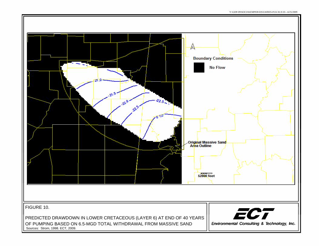
EUTAW-MCSHAN AQUIFER—LAYER 2
The Eutaw and McShan are considered a single aquifer because the sands are hydrauli-
cally connected. This aquifer outcrops in northeastern Mississippi and northwestern Ala-
bama. The upper portions of the aquifer are finer grained and contain a high silt content.
The lower portions of the aquifer consist of thin beds of glauconitic sand. Sand thickness
ranges from 1 ft in the eastern outcrop area to more than 300 ft to the southwest (Fig-
ure 7, Strom, 1998). Data collected from the onsite test well (Earth Science & Environ-
mental Engineering [ES&EE], 2007) indicate that the Eutaw-McShan aquifer and confin-
ing unit are 360 ft thick at the site with a total sand thickness of 150 ft.
Strom reports an average horizontal hydraulic conductivity of 12 ft/day was used in the
model based on 50 aquifer tests. Recharge to the aquifer is primarily due to precipitation
in the outcrop area. The Eutaw-McShan is separated from the overlying Coffee Sand by
the Mooreville Chalk to the south. Where the chalk is absent to the north, the Eutaw-
McShan is in contact with the Coffee Sand. However, the fine sediments of the upper
portion of the Eutaw-McShan function as an aquitard, hydraulically separating it from the
overlying Coffee Sand (Strom, 1998). Model transmissivity at the site location ranges
between 1,924 and 1,982 square feet per day (ft2/day).
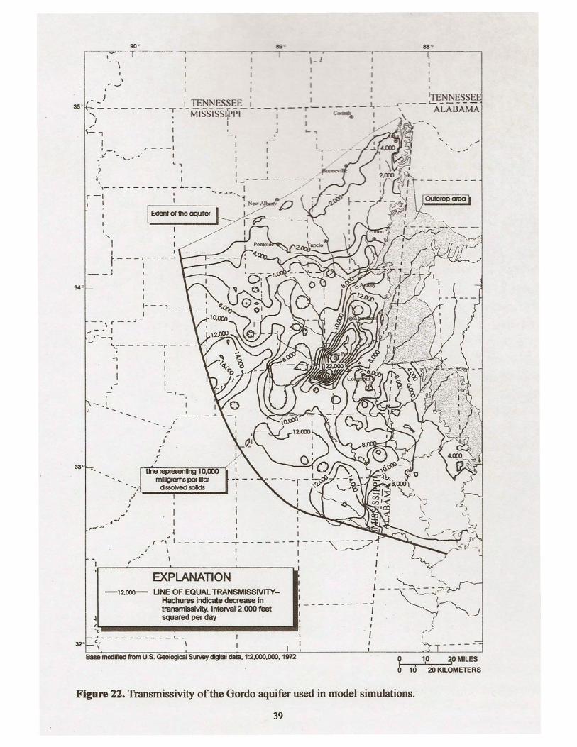
GORDO AQUIFER—LAYER 3
The Gordo aquifer outcrops in extreme northeastern Mississippi and northwestern Ala-
bama (Figure 8, Strom, 1998). The upper portion of the aquifer is interbedded sand and
clay, while the lower sections are composed of coarse-grained quartz sand and chert gra-
vel (Strom, 1998). Total sand thickness based on well log data ranges from 1 ft in the
eastern outcrop area to approximately 300 ft to the west (Figure 8, Strom, 1998). Recent

5 Y:\GDP-09\SOCO\KEMPER\GWRES.DOC—062609
data collected from the onsite ES&EE test well indicate that the Gordo aquifer and con-
fining unit are 470 ft thick at the site with a total sand thickness of 230 ft.
The average hydraulic conductivity defined in the Strom Model is 48 ft/day. This value
was reportedly based on 33 aquifer tests. The Gordo aquifer receives recharge from pre-
cipitation in the outcrop area. Recharge has also been reported from the overlying and
underlying aquifers according to Strom. The Gordo also is believed to discharge to topo-
graphic lows in the outcrop, the Coker in the updip area and the Eutaw-McShan in por-
tions of the down-dip area. A clay and silt layer (up to 175 ft thick in the southernmost
area of the model) separates the Gordo from the overlying Eutaw-McShan aquifer.
(Strom, 1998).
COKER AQUIFER—LAYER 4
The Coker aquifer does not outcrop in Mississippi, but does outcrop in northwestern Ala-
bama (Figure 9, Strom, 1998). The Coker consists of interbedded gray shale and lenticu-
lar beds of fine- to medium-grained sand. Strom reports that the total thickness of the
Coker aquifer based on well log data ranges from 1 ft in the outcrop area to more than
300 ft in the western portion of the model area. Data collected from the ES&EE onsite
test well indicate that the Coker aquifer and confining unit are 520 ft thick at the site with
a total sand thickness of 120 ft. Model transmissivity at the site location in the Coker
aquifer ranges between 6,990 and 7,120 ft2/day.
Recharge to the Coker enters the aquifer from precipitation in the outcrop and from
ground water seepage from the overlying and underlying aquifers. The Coker may dis-
charge ground water to the Gordo in the down-dip area and to the massive sand in the up-
dip area. A clay and silt layer, up to 175 ft thick in the west, acts as an aquitard between
the Coker and the overlying Gordo aquifer.
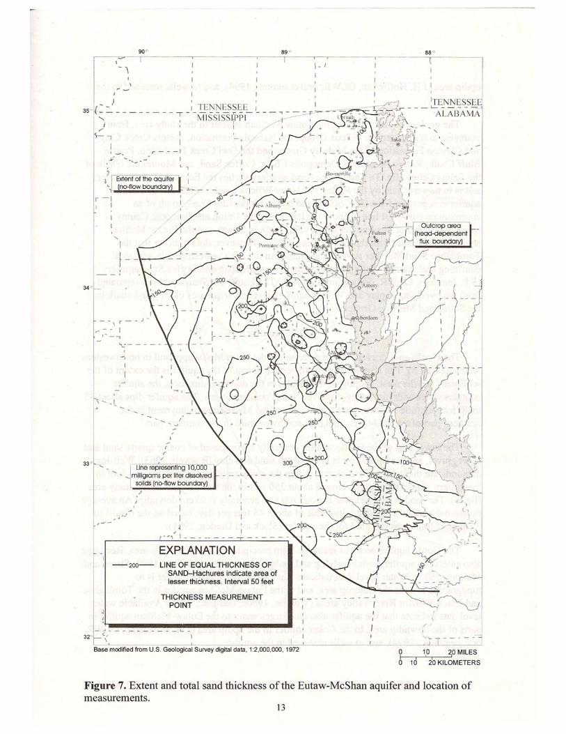
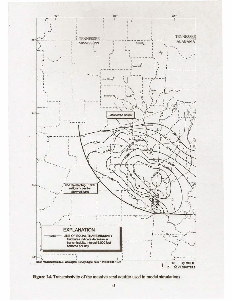
MASSIVE SAND AQUIFER—LAYER 5
The Massive Sand of the Tuscaloosa Group (Upper Cretaceous) has been selected as a
source of nonpotable water for the backup water supply for the facility. The Massive
Sand aquifer does not outcrop and is reported to be in contact with the Coker in the eas-

6 Y:\GDP-09\SOCO\KEMPER\GWRES.DOC—062609
ternmost areas of the model (Figure 10, Strom, 1998). A clay confining unit appears be-
tween the Coker and Massive Sand aquifers to the west that hydraulically separates the
aquifers. The Massive Sand consists of nonmarine medium- to coarse-grained, brown to
white sand with a lower zone of chert and quartz pea gravel. Sand thickness reported by
Strom based on well log data ranges from 1 ft in the eastern portion of the model to more
than 300 ft to the south. Data collected from the ES&EE onsite test well indicate that the
Massive Sand aquifer and confining unit are 290 ft thick at the site with a total sand
thickness of 260 ft.
A horizontal hydraulic conductivity of 60 ft/day was used for the Massive Sand aquifer in
the down-dip portion of the model and approximately 120 ft/day in the up-dip areas
(Strom, 1998).
Aquifer testing in the upper portion of the Massive Sand aquifer was performed by
ES&EE at the power plant site. The test well has an 80-ft screen interval set from 3,362
to 3,442 feet below land surface (ft bls). Step drawdown and constant rate aquifer pump-
ing tests were conducted in this well. The constant rate aquifer test was performed for
48 hours at a pumping rate of 800 gallons per minute (gpm). A transmissivity estimate of
2,900 ft2/day was derived using the Hantush and Jacob (1955) analytical method. In addi-
tion, the results of the step drawdown test analysis yielded a transmissivity estimate of
4,400 ft2/day using the Hantush (1962) analytical method (ES&EE, personal communica-
tion, October 2008). These transmissivity results are reflective of the upper 80 ft of the
Massive Sand aquifer, whereas the total thickness of the Massive Sand aquifer is approx-
imately 290 ft at the power plant site.
Using the total Massive Sand thickness of 260 ft, as determined in the test well, and the
60-ft/day horizontal hydraulic conductivity value representative of the entire Massive
Sand aquifer used by Strom (1998), an estimated transmissivity of 15,600 ft2/day is cal-
culated for the site location. The site area was originally defined in the Strom Model as
no-flow cells. Therefore, transmissivity values for the extended Massive Sand area were
defined based on transmissivity information published in Strom and Mallory, 1995, and
the ES&EE onsite well tests. Slightly conservative transmissivity values of 15,200 and

7 Y:\GDP-09\SOCO\KEMPER\GWRES.DOC—062609
15,300 ft2/day were assigned to the model cells representing the location of the proposed
withdrawal wells.
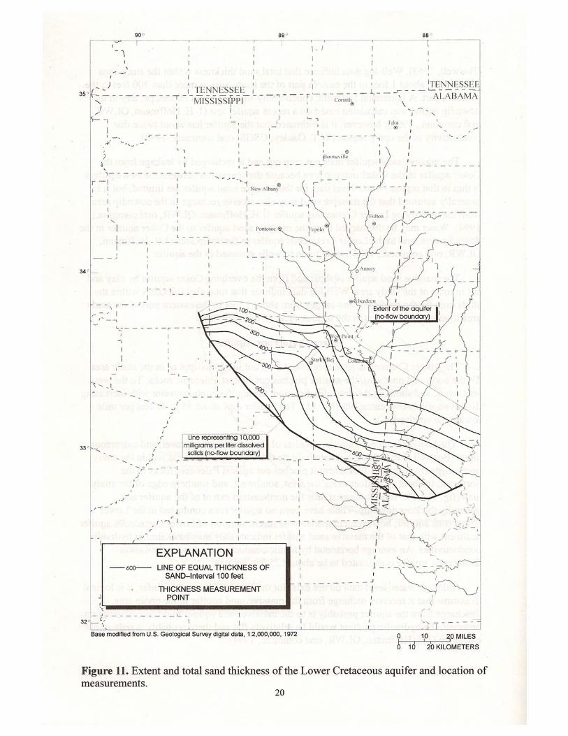
LOWER CRETACEOUS AQUIFER—LAYER 6
The Lower Cretaceous aquifer does not outcrop in the model area. The aquifer pinches
out toward the northeast and thickens toward the southeast (Figure 11, Strom, 1998). The
Lower Cretaceous aquifer consists of shale, clay, sand, gravel, and calcareous sediments.
Aquifer thickness based on well log data ranges from 1 ft in the northeast to more than
1,000 ft to the southwest (Figure 11, Strom 1998). The total thickness of the Lower Cre-
taceous at the site location is approximately 1,500 ft with a total sand thickness of
1,000 ft.
The Lower Cretaceous aquifer is believed to have similar hydraulic properties as the
Massive Sand. An average hydraulic conductivity of 125 ft/day is estimated by Strom.
The model cells corresponding to the site location are defined as no-flow cells in the
Lower Cretaceous (Layer 6). Model transmissivity in this layer increases going south-
westward from the outcrop area and ranges between 94,510 to 104,800 ft2/day at the edge
of the active model cells to the northeast of the site.
The Lower Cretaceous likely receives recharge from the Massive Sand aquifer in the up-
dip area and discharges to the Massive Sand aquifer down-dip. A confining unit consist-
ing of clay and silt up to 150 ft in the south has been identified above the Lower Creta-
ceous aquifer (Strom, 1998).
PALEOZOIC AQUIFER
For descriptions of the Iowa and Devonian aquifers, which are located in the northern-
most portion of the model area, refer to Strom (1998).
MODEL GRID DESIGN
The Strom Model covers 34,960 mi2 primarily in northeastern Mississippi but includes
portions of northwestern Alabama, southwestern Tennessee, and eastern Alabama. The
grid is oriented north-south with a 5,280- by 5,280-ft grid spacing. The lateral anisotropy

8 Y:\GDP-09\SOCO\KEMPER\GWRES.DOC—062609
used in the simulation was one. Each of the six grid layers consists of 230 rows and
152 columns (Figure 17, Strom, 1998).
GROUND WATER FLOW MODEL
ECT obtained a copy of the original Strom Model MODFLOW files that were used as the
base for an expanded model. The original 1998 model files were imported into the
ground water modeling software program Ground Water Vistas, where the simulations
were run using the 1988/1996 version of MODFLOW.
The Strom Model is a transient model constructed with six layers, with each layer
representing a regional aquifer as follows:
• Layer 1 is the Coffee Sand aquifer.
• Layer 2 is the Eutaw-McShan aquifer.
• Layer 3 is the Gordo aquifer.
• Layer 4 is the Coker aquifer.
• Layer 5 is the Massive Sand aquifer.
• Layer 6 is the Lower Cretaceous aquifer.
In the extreme northeastern corner of Mississippi, Layers 4 and 5 represent the Iowa
aquifer and the Devonian aquifer, respectively; the Coker and Massive Sand aquifers do
not extend to that area. Figure 18 (Strom, 1998) from Strom’s report illustrates the over-
lapping nature of the aquifer layers.
There is a thick, impermeable sequence comprising the Selma Group above Layer 1, the
Coffee Sand aquifer; therefore, the area overlying the Coffee Sand was simulated as no-
flow (black cell boundary color). Layer 1 does represent the Coffee Sand in the northern
portions of the model but is also used as an upper constant head boundary (dark blue cell
boundary color) for the Eutaw-McShan aquifer (Layer 2). The constant heads in this area
represent the surficial water levels on the chalk and clay overlying the Eutaw-McShan.
However, vertical flow is limited due to the low vertical hydraulic conductivity of the
confining unit (Strom, 1998).

9 Y:\GDP-09\SOCO\KEMPER\GWRES.DOC—062609
The boundaries for each subsequent aquifer/model layer are defined by both the deposi-
tional or erosional extent of the aquifer and by the location of the freshwater-saltwater
interface in the aquifer, which is defined by Strom as a total dissolved solids (TDS) con-
centration of 10,000 milligrams per liter (mg/L). The freshwater-saltwater interface
represents no-flow lateral boundaries in the Strom Model for all of the aquifers/layers; all
model cells located beyond the boundary are defined as no-flow boundaries and therefore
are inactive. However, the proposed well field for the power plant is located approx-
imately 4 miles south of (beyond) the published freshwater-saltwater boundary for the
Massive Sand aquifer (Layer 5) and is thus situated in an inactive portion of Layer 5.
Therefore, for the extended model boundaries, it was necessary to modify the Strom
Model in only one way: Layer 5 (the Massive Sand aquifer) was extended further to the
southwest, as shown in Figure 2. Representative values for transmissivity, as noted pre-
viously, were also defined for the extended Massive Sand aquifer area. No other changes
were made to model boundaries or cell input parameters relative to the Strom Model in
the initial expanded simulation.
Strom’s calibrated transient model includes pumping stresses for numerous wells from
1900 through 1995, which is the last year modeled by Strom. The extended model con-
tinues the 1995 pumping stresses forward in time (1996 through 2010) and then adds a
constant 1-MGD ground water withdrawal from the Massive Sand aquifer equally split
between two wells pumping at a rate of 66,850 cubic feet per day (ft3/day) at the power
plant site for a 40-year period, while continuing the 1995 withdrawal rates at the numer-
ous other wells (per Strom’s model). As such, the expanded model was used to simulate
the effects of the proposed 1-MGD ground water withdrawal over the projected 40-year
life of the facility. All wells are entered into the models as cells representing well boun-
dary conditions (red cell boundary).
RECHARGE
Based on reports from the National Oceanic and Atmospheric Administration (NOAA)
included in the Strom (1998) report, the area of northeastern Mississippi can receive an
average of 52 inches of precipitation in the outcrop areas along the northeastern sections

Y:\GDP-09\SOCO\KEMPER\EIS\GWRES-FGS.XLS\2—6/25/2009
FIGURE 2.
MASSIVE SAND (LAYER 5) ACTIVE CELL EXTENSION TOWARD SW OVER SITE PROPOSED WELLS LOCATED SW OF SALTWATER-FRESHWATER BOUNDARY Sources: Strom, 1998. ECT, 2009.
dmansell
Text Box
10

11 Y:\GDP-09\SOCO\KEMPER\GWRES.DOC—062609
of the Strom Model. The Strom Model simulates the intermediate and regional scale
flow. The outcrop areas of the Coffee Sand, Eutaw-McShan, Gordo, and Coker aquifers
were simulated with head-dependant flux boundaries (green cell boundary) using the riv-
er package in MODFLOW. Strom reports that the large base flows observed in even the
small streams in the outcrop area indicate that recharge from precipitation-rich environ-
ment is sufficient to provide all the recharge that the aquifers can accept and much of the
recharge is redirected as runoff.
STROM MODEL PARAMETERS AND CALIBRATION
The Strom Model calibration was based on transient conditions because of the lack of
water level data in the predevelopment stage. Initial transmissivity grids were created by
multiplying sand thickness data from well logs information with hydraulic conductivity
data collected from aquifer tests. The Strom Model initial transmissivity grids were mod-
ified within a range of expected values during model calibration. Contour maps for the
transmissivity values used in the Strom Model are illustrated on Strom’s Figures 20
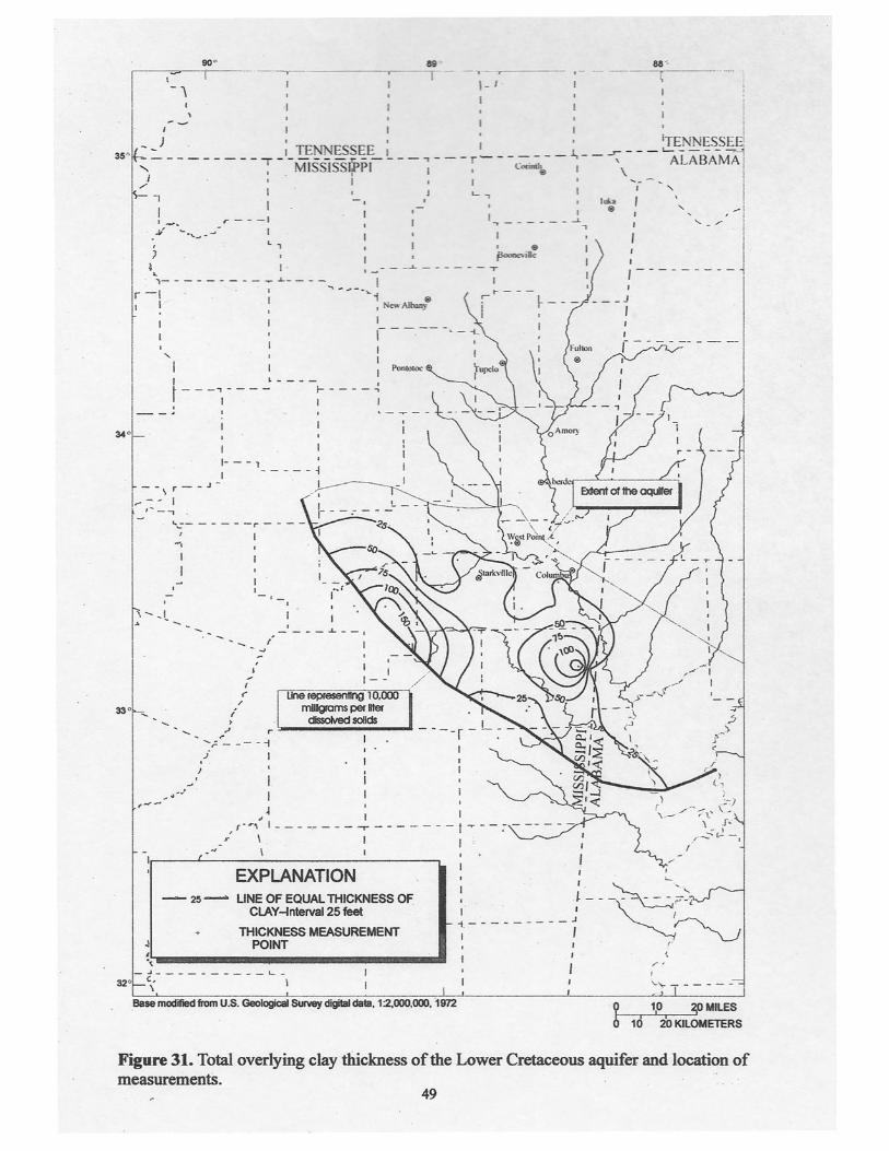
through 24 (Strom, 1998). Contour maps of the confining unit thickness are illustrated on
Strom’s Figures 27 through 31 (ibid.). A constant storage coefficient of 0.0001 was used
for all aquifers with the exception of the Gordo, which used a constant value of 0.001 to
represent the coarser grained material. There was no water level data in the Lower Creta-
ceous for calibration (ibid.).
An examination of the original Strom Model files indicated that the leakance value be-
tween the each confining unit and underlying aquifer was defined as 5.0 × 10⁻⁹ in the vi-
cinity of the site location. As defined, the leakance values are two orders of magnitude
lower than defined in an earlier model completed in the same area (Strom and Mallory,
1995) with the exception of the leakance between the Coffee Sand confining unit and the
underlying Eutaw-McShan. As noted previously, the only changes made to the Strom
Model were associated with the extension of the active cell area toward the southwest in
the Massive Sand aquifer (Layer 5). However, an additional 1.0-MGD test simulation
was run to check the sensitivity of the drawdown predictions to the leakance values. For
the test simulation, the Strom Model leakance values in the vicinity of the site were re-

12 Y:\GDP-09\SOCO\KEMPER\GWRES.DOC—062609
vised from 5.0 × 10⁻⁹ in Layers 2, 3, 4, and 5 to 2.0 × 10⁻⁷, 1.0 × 10⁻⁷, 3.0 × 10⁻⁷,
5.0 × 10⁻⁷, respectively.
MODEL RESULTS
The 1.0-MGD model was first run without the addition of the two proposed pumping
wells. Wells withdrawing at a rate of 0.5 MGD each were added in model cells R182 C92
and R183 C92, and the simulation was rerun. Drawdown was then computed by subtract-
ing the head data from the initial simulation from the head data generated from the
second simulation containing the proposed well withdrawals. The resulting drawdown
after 40 years of pumping was contoured.
Figure 3 depicts the potentiometric surface drawdown estimated in the Massive Sand
aquifer after 40 years of constantly pumping at the 1-MGD rate. The estimated draw-
downs are widespread, yet of a low magnitude. The expanded model estimates approx-
imately 6 ft of drawdown at the nearest existing user of the Massive Sand aquifer, which
is located approximately 9.5 miles northeast of the proposed power plant in the town of
De Kalb. The Mississippi Department of Environmental Quality (MDEQ) water well da-
tabase (MDEQ, August 2008) suggests that several wells using the Massive Sand aquifer
exist near the towns of Electric Mills and Scooba. Those wells are located approximately
21 to 22 miles east-northeast of the power plant site, and less than 5 ft of drawdown is
predicted in the Massive Sand (Layer 5) at those well locations. These estimated draw-
downs (6 ft or less) are not expected to cause any adverse impact to existing users of the
water from the Massive Sand aquifer.
Smaller drawdowns would occur in the underlying and overlying aquifers. The expanded
model estimated maximum drawdowns are 3.5 ft or less drawdown in the underlying
Lower Cretaceous aquifer (Layer 6) as shown on Figure 4. Less than 3 ft of drawdown is
predicted in the overlying Coker aquifer (Layer 4), as shown on Figure 5. A maximum of
1.5 ft of drawdown is predicted in the Gordo aquifer (Layer 3), with the highest draw-
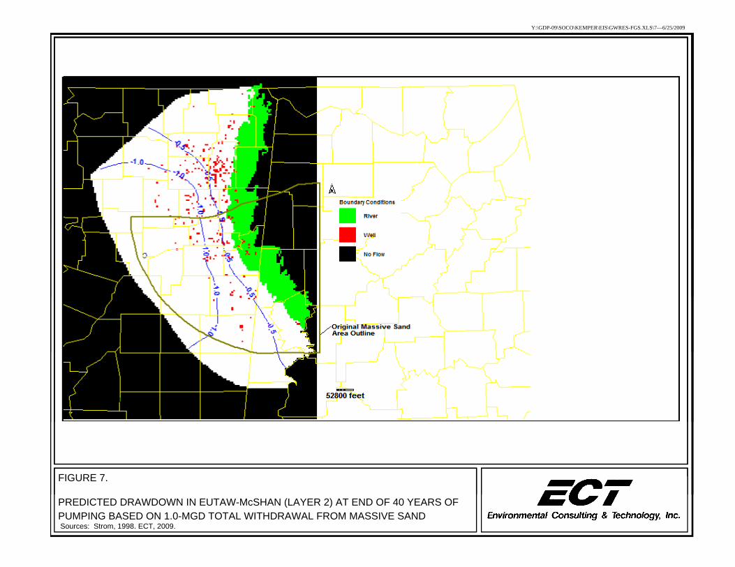
down observed along the western edge of the aquifer (Figure 6). A similar drawdown pat-
tern is displayed for the Eutaw-McShan aquifer (Layer 2), with a maximum of 1.5 ft or
less of drawdown (see Figure 7). Less than 1 ft of drawdown is predicted in the

Y:\GDP-09\SOCO\KEMPER\EIS\GWRES-FGS.XLS\3—6/25/2009
FIGURE 3.
PREDICTED DRAWDOWN IN MASSIVE SAND (LAYER 5) AT END OF 40 YEARS OF PUMPING BASED ON 1.0-MGD TOTAL WITHDRAWAL FROM MASSIVE SAND Sources: Strom, 1998. ECT, 2009.
dmansell
Text Box
13

Y:\GDP-09\SOCO\KEMPER\EIS\GWRES-FGS.XLS\4—6/25/2009
FIGURE 4.
PREDICTED DRAWDOWN IN LOWER CRETACEOUS AT END OF 40 YEARS OF PUMPING BASED ON 1.0-MGD TOTAL WITHDRAWAL FROM MASSIVE SAND Sources: Strom, 1998. ECT, 2009.
dmansell
Text Box
14

Y:\GDP-09\SOCO\KEMPER\EIS\GWRES-FGS.XLS\5—6/25/2009
FIGURE 5.
PREDICTED DRAWDOWN IN COKER (LAYER 4) AT END OF 40 YEARS OF PUMPING BASED ON 1.0-MGD TOTAL WITHDRAWAL FROM MASSIVE SAND Sources: Strom, 1998. ECT, 2009.
dmansell
Text Box
15

Y:\GDP-09\SOCO\KEMPER\EIS\GWRES-FGS.XLS\6—6/25/2009
FIGURE 6.
PREDICTED DRAWDOWN IN GORDO (LAYER 3) AT END OF 40 YEARS OF PUMPING BASED ON 1.0-MGD TOTAL WITHDRAWAL FROM MASSIVE SAND Sources: Strom, 1998. ECT, 2009.
dmansell
Text Box
16
Y:\GDP-09\SOCO\KEMPER\EIS\GWRES-FGS.XLS\7—6/25/2009
FIGURE 7.
PREDICTED DRAWDOWN IN EUTAW-McSHAN (LAYER 2) AT END OF 40 YEARS OF PUMPING BASED ON 1.0-MGD TOTAL WITHDRAWAL FROM MASSIVE SAND Sources: Strom, 1998. ECT, 2009.
dmansell
Text Box
17

18 Y:\GDP-09\SOCO\KEMPER\GWRES.DOC—062609
simulation for the upper layer (Layer 1), the Coffee Sand (Figure 8). Generally, there is
an increase in drawdown in the Coker, Eutaw-McShan, Gordo, and Coffee aquifers to the
southwest, away from the recharge areas in the northeast portion of the model. The
MDEQ water well database (MDEQ, August 2008) suggests that, within 20 miles of the
proposed power plant site, no existing users of the water are present in the overlying
Coker aquifer or the underlying Lower Cretaceous aquifer.
The results of the test simulation, conducted to investigate the sensitivity of the model to
the lower leakance values defined in the vicinity of the site, did not indicate any change
to the drawdown predicted in the Coffee Sand aquifer, Eutaw-McShan aquifer, or Gordo
aquifer (Layers 1, 2, and 3, respectively). A slight decrease of 0.3 ft and 0.1 ft was ob-
served in the Massive Sand aquifer (Layer 5) and the Lower Cretaceous aquifer
(Layer 6), respectively. The drawdown changes in the Massive Sand aquifer (Layer 5)
were limited to the area immediately adjacent to the proposed well and the southwestern
freshwater-saltwater boundary.
Consideration was also given to the potential effects of the proposed withdrawal of
1 MGD on ground water quality. The Massive Sand aquifer at the site is known to be sa-
line (e.g., the TDS concentration is 23,000 mg/L); as such, the site is situated on the salt-
water side of the freshwater-saltwater interface as defined by 10,000 mg/L TDS. The es-
timated drawdowns do not suggest the likelihood for inducing any measurable saltwater
migration into freshwater potions of any aquifer.
Based on the modeling assumptions and the fact that the actual ground water withdrawals
will be on an as-needed basis, the 1-MGD model drawdown predictions are conservative.
Therefore, the modeling results suggest that the withdrawal of 1 MGD of ground water
from the Massive Sand aquifer will not cause any adverse impact to existing users of the
water from the various underlying and overlying aquifers.
ALTERNATIVE 6.5 MGD SIMULATION
To evaluate the effect of using the well field to supply the entire 6.5-MGD water re-
quirement of the facility, an additional simulation was run keeping all other parameters

Y:\GDP-09\SOCO\KEMPER\EIS\GWRES-FGS.XLS\8—6/25/2009
FIGURE 8.
PREDICTED DRAWDOWN IN COFFEE SAND (LAYER 1) AT END OF 40 YEARS OF PUMPING BASED ON 1.0-MGD TOTAL WITHDRAWAL FROM MASSIVE SAND Sources: Strom, 1998. ECT, 2009.
dmansell
Text Box
19
20 Y:\GDP-09\SOCO\KEMPER\GWRES.DOC—062609
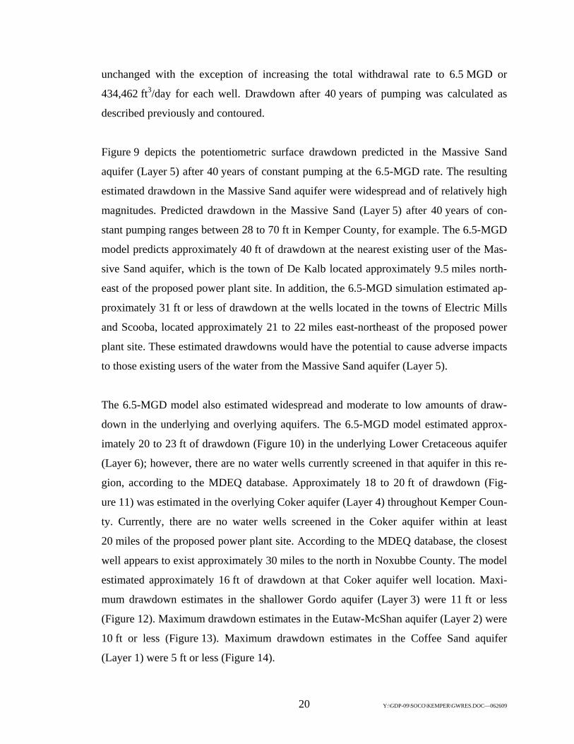
unchanged with the exception of increasing the total withdrawal rate to 6.5 MGD or
434,462 ft3/day for each well. Drawdown after 40 years of pumping was calculated as
described previously and contoured.
Figure 9 depicts the potentiometric surface drawdown predicted in the Massive Sand
aquifer (Layer 5) after 40 years of constant pumping at the 6.5-MGD rate. The resulting
estimated drawdown in the Massive Sand aquifer were widespread and of relatively high
magnitudes. Predicted drawdown in the Massive Sand (Layer 5) after 40 years of con-
stant pumping ranges between 28 to 70 ft in Kemper County, for example. The 6.5-MGD
model predicts approximately 40 ft of drawdown at the nearest existing user of the Mas-
sive Sand aquifer, which is the town of De Kalb located approximately 9.5 miles north-
east of the proposed power plant site. In addition, the 6.5-MGD simulation estimated ap-
proximately 31 ft or less of drawdown at the wells located in the towns of Electric Mills
and Scooba, located approximately 21 to 22 miles east-northeast of the proposed power
plant site. These estimated drawdowns would have the potential to cause adverse impacts
to those existing users of the water from the Massive Sand aquifer (Layer 5).
The 6.5-MGD model also estimated widespread and moderate to low amounts of draw-
down in the underlying and overlying aquifers. The 6.5-MGD model estimated approx-
imately 20 to 23 ft of drawdown (Figure 10) in the underlying Lower Cretaceous aquifer
(Layer 6); however, there are no water wells currently screened in that aquifer in this re-
gion, according to the MDEQ database. Approximately 18 to 20 ft of drawdown (Fig-
ure 11) was estimated in the overlying Coker aquifer (Layer 4) throughout Kemper Coun-
ty. Currently, there are no water wells screened in the Coker aquifer within at least
20 miles of the proposed power plant site. According to the MDEQ database, the closest
well appears to exist approximately 30 miles to the north in Noxubbe County. The model
estimated approximately 16 ft of drawdown at that Coker aquifer well location. Maxi-
mum drawdown estimates in the shallower Gordo aquifer (Layer 3) were 11 ft or less
(Figure 12). Maximum drawdown estimates in the Eutaw-McShan aquifer (Layer 2) were
10 ft or less (Figure 13). Maximum drawdown estimates in the Coffee Sand aquifer
(Layer 1) were 5 ft or less (Figure 14).

Y:\GDP-09\SOCO\KEMPER\EIS\GWRES-FGS.XLS\9—6/25/2009
FIGURE 9.
PREDICTED DRAWDOWN IN MASSIVE SAND (LAYER 5) AT END OF 40 YEARS OF PUMPING BASED ON 6.5-MGD TOTAL WITHDRAWAL FROM MASSIVE SAND Sources: Strom, 1998. ECT, 2009.
dmansell
Text Box
21
Y:\GDP-09\SOCO\KEMPER\EIS\GWRES-FGS.XLS\10—6/25/2009
FIGURE 10.
PREDICTED DRAWDOWN IN LOWER CRETACEOUS (LAYER 6) AT END OF 40 YEARS OF PUMPING BASED ON 6.5-MGD TOTAL WITHDRAWAL FROM MASSIVE SAND Sources: Strom, 1998. ECT, 2009.
dmansell
Text Box
22

Y:\GDP-09\SOCO\KEMPER\EIS\GWRES-FGS.XLS\11—6/25/2009
FIGURE 11.
PREDICTED DRAWDOWN IN COKER (LAYER 4) AT END OF 40 YEARS OF PUMPING BASED ON 6.5-MGD TOTAL WITHDRAWAL FROM MASSIVE SAND Sources: Strom, 1998. ECT, 2009.
dmansell
Text Box
23

Y:\GDP-09\SOCO\KEMPER\EIS\GWRES-FGS.XLS\12—6/25/2009
FIGURE 12.
PREDICTED DRAWDOWN IN GORDO (LAYER 3) AT END OF 40 YEARS OF PUMPING BASED ON 6.5-MGD TOTAL WITHDRAWAL FROM MASSIVE SAND Sources: Strom, 1998. ECT, 2009.
dmansell
Text Box
24

Y:\GDP-09\SOCO\KEMPER\EIS\GWRES-FGS.XLS\13—6/25/2009
FIGURE 13.
PREDICTED DRAWDOWN IN EUTAW-McSHAN (LAYER 2) AT END OF 40 YEARS OF PUMPING BASED ON 6.5-MGD TOTAL WITHDRAWAL FROM MASSIVE SAND Sources: Strom, 1998. ECT, 2009.
dmansell
Text Box
25

Y:\GDP-09\SOCO\KEMPER\EIS\GWRES-FGS.XLS\14—6/25/2009
FIGURE 14.
PREDICTED DRAWDOWN IN COFFEE SAND (LAYER 1) AT END OF 40 YEARS OF PUMPING BASED ON 6.5-MGD TOTAL WITHDRAWAL FROM MASSIVE SAND Sources: Strom, 1998. ECT, 2009.
dmansell
Text Box
26

27 Y:\GDP-09\SOCO\KEMPER\GWRES.DOC—062609
The 6.5-MGD simulation suggests that these estimated drawdowns have the potential to
cause adverse impacts to existing Massive Sand aquifer users and would have some po-
tential to cause minor adverse impact to existing users of ground water from the Coker
and possibly the Gordo aquifers. No significant impacts would be expected relative to the
existing users of ground water from the Eutaw-McShan aquifer or the Coffee Sand aqui-
fer. Actual impacts to a water user’s well are relative not only to the amount of draw-
down experienced but also to the specific construction and condition of each well. How-
ever, such impacts could likely be mitigated by retrofitting and/or upgrading well pumps
at impacted wells.
MODEL LIMITATIONS AND DISCUSSION
The southwest boundary of the model layers have been defined as a sharp contact
representing the freshwater to the northeast of the boundary and the saline ground water
to the southwest of the boundary. While this freshwater-saltwater boundary is typically
represented as a sharp contact in ground water flow modeling, implying that the fluids are
immiscible liquids, this is not actually correct. The transition zones between fresh and
saline ground water can vary between a few tens of feet to more than a few miles.
The proposed wells will be withdrawing from the saline portion of the Massive Sand
aquifer approximately 3 to 4 miles to the southwest of the freshwater-saltwater boundary
defined for the area by Strom (1998). The location of the existing freshwater-saltwater
boundary is based on the equilibrium of the ground water flow system. Placing pumping
wells close to this boundary will change this equilibrium and likely cause a shift in the
boundary location. The variable dissolved solid concentrations found in the saline ground
water affects the ground water density and consequently ground water flow. MOD-
FLOW, a single density fluid model, does not account for variable density affects that
would occur in the vicinity of the freshwater-saltwater boundary. The Strom Model and
expanded 1.0-MGD model, therefore, are not designed to estimate the movement of the
freshwater-saltwater boundary or consider spatial variations in fluid density that can af-
fect ground water flow and predicted drawdown.

28 Y:\GDP-09\SOCO\KEMPER\GWRES.DOC—062609
The actual head values in the saline portion of the aquifer (at equal elevation/pressure)
would be lower than predicted by the current MODFLOW simulations, which only calcu-
late head distributions based on freshwater/low density ground water. Based on the po-
tential gradients the actual lower head values would tend to induce and considering the
modeling performed for the Red Hills Final Environmental Impact Statement (TVA,
1998) under similar circumstances of pumping, position relative to the freshwater-
saltwater interface, and hydrogeologic conditions, it is likely that the boundary would
migrate on the order of 1,000 to 2,000 ft to the southwest. This would expand the transi-
tion zone and/or the freshwater section of the Massive Sand aquifer toward the southwest
in the vicinity of the proposed power plant. In addition, the current MODFLOW simula-
tions will slightly overestimate the drawdown observed at greater distances from the
freshwater-saltwater boundary and toward the recharge areas and underestimate the
drawdown in the vicinity of the site.
The Strom Model was developed using average heads calculated for the entire 1-mi2 cell
area and therefore should be used for analyzing ground water flow on a regional scale.
Transmissivity and other hydraulic properties of the aquifers modeled are assumed to be
constant within each 1-mi2 grid cell. Therefore, the expanded model is valid as a regional
assessment tool.
The hydraulic property data (transmissivity, leakance, hydraulic conductivity, etc.) used
to develop the Strom Model is limited to wells drilled before 1995. There are likely other
new wells, in addition to the ES&EE onsite test well, that could provide updated hydrau-
lic property data that may have an impact on the model predictions.
No-flow boundaries have been used to define the layer boundaries at the depositional
edge of the aquifers and at the freshwater-saltwater boundary. In reality, the up-dip, de-
positional edges of the aquifers may not be isolated but rather in contact with other satu-
rated sediments. Similarly, the fresh and saline ground waters are not truly immiscible
fluids, so there will likely be some degree of flow associated with the freshwater-
saltwater boundary. These conditions will tend to cause the 1.0-MGD model to slightly
overestimate the predicted drawdown.

29 Y:\GDP-09\SOCO\KEMPER\GWRES.DOC—062609
Since only the southwestern extent of the Massive Sand aquifer (Layer 5) was extended
to include active cells in the area of the proposed wells, the cells in the Layers 3 and 6
above and below the extension remain no-flow cells. While active cells are present in the
Coker aquifer (Layer 4) overlying the proposed site wells, they are only a few miles from
the freshwater-saltwater boundary defined in that layer. This may cause a slight overes-
timation in the drawdown in the Massive Sand aquifer (Layer 5) and Lower Cretaceous
(Layer 6) and an underestimation in the drawdown in the overlying Layers 3 and 4, the
Gordo and Coker aquifers, respectively. However, at the 1.0-MGD pumping rate, the re-
sulting effects on the predicted drawdown is expected to be insignificant.
Similarly, the low leakance values of 5.0 × 10⁻⁹, used in the Strom Model over much of
the west and southwest portion of the aquifers, is two orders of magnitude lower than
would be expected based on information published leakance values for an earlier USGS
MODFLOW simulation completed in the same area (Strom and Mallory, 1995). The test
simulation indicates that this lower leakance value tends to overestimate the drawdown
predicted in the Massive Sand aquifer (Layer 5) and Lower Cretaceous aquifer (Layer 6).
The effect of the lower leakance value on the predicted drawdowns for the 1.0-MGD
model is expected to be insignificant.

30 Y:\GDP-09\SOCO\KEMPER\GWRES.DOC—091709
REFERENCES Anderson, M.P., and Woessner, W.W. 1992. Applied Ground Water Modeling: Simula-
tion of Flow and Advective Transport. Academic Press, Inc., New York, 381 pp. Earth Science & Environmental Engineering (ES&EE), Southern Company Generation.
2007. Preliminary Subsurface Investigation Report, Integrated Gasification Com-bined Cycle Plant, Kemper County, Mississippi.
Hantush, M.S. 1962. Flow of Ground Water in Sands of Nonuniform Thickness, 3. Flow
to Wells. Jour. Geophys. Res. Vol. 67, No. 4. Hantush, M.S., and Jacob, C.E. 1955. Non-Steady Radial Flow in an Infinite Leaky Aqui-
fer. American Geophysical Union Transactions. Vol 36. McDonald, M.G., and Harbaugh, A.W. 1996. User’s Documentation for MODFLOW-96,
An Update to the U.S. Geological Survey Modular Finite-Difference Ground-Water Flow Model. USGS Open-File Report 96-485.
———. 1988. A Modular Three-Dimensional Finite-Difference Ground-water Flow
Model. U.S. Geological Survey (USGS) Techniques of Water-Resources Investiga-tions Report, Chapter 6-A1, 586 pp.
Mississippi Department of Environmental Quality (MDEQ). August 2008. Water Well
Database. Transmitted from MDEQ to ECT on August 22. Strom, E.W. 1998. Hydrogeology and Simulation of Ground Water Flow in the Creta-
ceous-Paleozoic Aquifer System in Northeastern Mississippi, U.S. Geological Survey, Water-Resources Investigations Report, No. 98-4171.
Strom, E.W., and Mallory, M.J. 1995. Hydrogeology and Simulation of Ground Water
Flow in the Eutaw-McShan Aquifer and in the Tuscaloosa Aquifer System in Nor-theastern Mississippi. U.S. Geological Survey Water Resources Report, No. 94-4223.
Tennessee Valley Authority (TVA). 1998. Red Hills Power Project Final Environmental
Impact Statement. July.

APPENDIX A
STROM MODEL REPORT FIGURES

.--
, : ~'-'
~-.- ..-----;-.~~I (
I <//
_J L_ I I
32" C, I "'- - -\ I I~-i--~~--~~~~~~----~~-~~~~~~~-~,--------------~----------~~I-L---Base modified from U.S_ Geological Survey digital data, 1:2,000,000,1972 0 1,0 2,0MILES
b 1d 2'0KILOMETERS
35
r
89
fExte~tct the aqUife-r-- ;-- T -- '\ ~(no-flowboundary), I
--1-- -\--1 - --- ---,--
,-- 880---- --r,- ----I
~ 50 ,-:. SEE I
- - - - - - - -:- - -l\IIISS1SS{PB-100 , '
l ukaGl
0200
Depositionalextentof the oqurer
(no-flowboundary)
rTr:=--====-'=,..,,-""".,...._ _ -I II I
/
;,
--'- , II
- ~ I Ir -'\ I - - - -- - - - -,- - - - - - - - I - - - - - - - - - -I
EXPLANATION I I
)r \ »)\-/-'-;:\",\",
\ ) c
/ --...::. (.~ -./
\
, - 50 - LINE OF EQUAL THICKNESS OFSAND-Hachures indicate area oflesser thickness. Interval 50 feet
THICKNESS MEASUREMENTPOINT
Figure 6. Extent and total sand thickness of the Coffee Sand aquifer and location ofmeasurements.
11
900 88C
I
\
l- J
I
-,
" - ) I TEN ESSEE I35 ~- - - - - - - - - - T - - - - - - r - - - - - ., - - -
<, ,MISSISS],PPI ..-f~-/) • ; // J
- -,, -.-,,' ........ --'
r - - -IIL 1
I,--;o--;---;-;--;,------,,------c• Extent of the aquifer'i-..n,;;o;,,;-fiiilo;,;w;.;,bo••u;;;n.d;,;a;,ry"-.t:--:L----- __
r -I II I
,~--------
"-III- -r-
IJ"'_-,
"'"---- - - - -
I- ..,
Ir
/
330
""' Line representlng 10,000'- - <, milligrams per liter dissolved
solids [no-flow boundary).J I
F',
EXPLANATION- 200- LINE OF EQUAL THICKNESS OF
SAND-Hachures indicate area oflesser thickness. Interval 50 feet
THICKNESS MEASUREMENTPOINT
32"
_...J L._
C,'. I
Base modified from U.S. Geological Survey digital data, 1 :2,000,000, 1972 ob
1,0 30 MILES
10 2'0 KILOMETERS
Figure 7. Extent and total sand thickness of the Eutaw-McShan aquifer and location ofmeasurements.
13

00 ~. ~"
I -~~- -r-'- --; ; T - l:~.: ; - ~ - -'II' I I ; I I
II I I I'
- _J ; TE lESSEE; ; '_r- !E~~~S5~EI35 f~ - - - - - - - - - - - - - - - - r - - - - - -, - - - r - - - - - - - 1, - - ALABAMA
f" I MISSISSf:PP1 I CNIIIIIl;, I \) I -,- -1 L... ,
I '"r - - -I
I, -.-,,'
L ,,)
l~"'!- ..•....J..._ _ _ _ Ir-I : "~-'--~i Gl
I I Extentof the aquifer ' ' C" AJ9'n~1/'/ ....
(no-flow boundary) ~'--.••..•,.....•..••..•.•.••....----.I--I1+\-'.f>
II -> - - -~ - - - - - - ..•
,<,
IIf - - -, - - - -I I,
34"
II" _-,
-,
II'"'f ,
/
I('
/33" Line representing 10,000
milligrams per literdissolved<, r solids(no-flow boundary)--' I
EXPLANATION, -250- LINE OF EQUAL THICKNESS OF
SAND-Hachures indicate area oflesser thickness. Interval 50 feet
, I ~"~---------!--~~I rI (
/'/,
THICKNESS MEASUREMENTPOINT
_J L_
C,\
Base modified from U_R Geological Survey digital data, 1:2,000,000. 1972 o 1,0 30 MILESb 10 2'0 KILOMETERS
Figure 8. Extent and total sand thickness of the Gordo aquifer and location ofmeasurements.
15

I
- ) l-ENINESSEE I ' ITENNESSEE,.r - I -, '~I _l ,---L-----~~35\-~---------T------r-----,---r·------ , \ ALI\.BAMI\.
<, MISSISSIPPI I Cortnth I \ •• II I' lIe I
/ I I '- - - " ')- -1 '- , I uka I
! __ . r---I -r ~ e ",- ~I...1/ -v .•. ~ -' I -t
900,-=-~----, ..-
'- "\ :, I,
89'1-
\- I
I
88 "- --r'
"
f L 1 I 0I 1 f,30tlllc"illc1 l I .....•---....L------T. \- ~ L_ _ _ _ Ir-I' . I ..,~-·--~iI I I NewAlban)~
<,
IIf - - -, - - - -I I
I- - - ---I ' - -1
II
Extent of the aquifer Pontotoc •, -no-flow boundary
I"" - - - ~ J
, II
~t\.__---- I l',_ ..::~~-,
l..•.••-_ - - - - - r - - -r
33°
II-'- ,
,.;~- .~
- - ,, II :
\ ~ .1
(
('
/
Line representing 10.000milligrams per liter dissolvedsolids (no-flow boundary)
.J,
II
" ~ I Ir . T\ I __ _-- _ __ ...,..._ __ - - - - I ~ -
r,I ' -150- LINE OF EQUALTHICKNESS OF, I •
SAND-Hachures indicate area of I ~ -
I T~~~~;;:=::~:::~:;~t~..._._.._.-;-.~~32
01- ;. _ . _ .... _ . _ L .\ : •
~'. I ~~~~1~7~----------~-----------~~~~~T--"_-_-- :]Base modified from U.S. Geological Survey digital data. 1:2.000.000. 1972
EXPLANATION !
o 1,0 30 MILES
b 1d 2'0 KILOMETERS
Figure 9. Extent and total sand thickness ofthe Coker aquifer and location ofmeasurements.
17
--- -, 89'T
880-':~/----'---~~--:J' , , , '
) " , ~TE~'\I_N~SS_EE35 l.-=:'" - - - - - - - - T -'- I.Et:Jt:J~~EiE_,_ - - -t - - - I~- - - - - - _1,_ - -\ -ALAB-A-MA
<, MISSISSIPPI I Corinth I \I ' ill
/' 'J ',- - - -,- -1 I 1- .,
- -"----
,,
r - - -I I '.,. -1.
-t,lukaill
I L 1 I 0) ,/300"0' illc1 I I__---....L------,\- -:- .l- '"" .,. ~. _ ~ I
r -I I "i illI I ! New Alban)
1----
r ~-------J, III ;------,-"
I-, I : I'ontoroc e, '----L ,~
Ir---',---- ,
--.I I
r - - - - -- - -- --
t'" _-,
L......::-_ - - - - -r - - -
~,
,I-,
\ ~ -L
I- -J
33°
(
r ,Line representing 10,000
: milligrams per liter dissolved.J solids (no-flow boundary)
r:-r - - - --Ii
• .1II
, ~ I Ir . r\ ,- - - -- - - - ...•- - - - - - - t - - - ~ - - - - - - - ,
/ --•..•..•. ~ -.EXPLANATION
-250- LINE OF EQUAL THICKNESS OFSAND-Hachures indicate area oflesser thickness. Interval 50 feet
THICKNESS MEASUREMENTPOINT
_ J:-_ •••••••••• _·_ •• _•• _~L·_••••••••••••~,••••••••••••c,: I
Base modifted from U.S. Geologica' Survey digital data, 1:2,000,000, 1972 o 1,0 2,0 MILES
b 10 2'0 KILOMETERS
Figure 10. Extent and total sand thickness of the massive sand aquifer and location ofmeasurements.
18
900 89°'"--"'-r---,---rI \ _ I
I
880------'\'I,
\
33°
'- -r
,'" - I I ~ I
- ) , TENINESSEE I, I ' ITENNESSEE( - I " - _. I 1 r-' L- _
35C' \-~ - - - - - - - - - T - - - - :...- r: - - - - - ., - - - r'- - - - - - - 1 - - - \ ALABAMA
<, MISSISS]'PPI I C"'intl~ I \) i ',- - - -,
..J,..... •... •. " •..• _-'
luka®
t L ., I €I
) I /300no\' ilie1 I .---' ....1- -r-
\ ~.L_---'"'--.-- Ir -I h'1 ® t- - - - I ,
I I NewAlbany r - - - - - - - -1 II
I1- - - -- -, - ~I-, I
I I Pcmotocef - - -'1 - - - .: - - - -I- - - - - ~
,
r - - - - -- - -- --
I, .... _--,1.,...,:-- - - - - -r - - - - \-1----.....
-,
. I
r- .j
I('
/
I I1--
Line representing 10,000milligrams per I~er dissolvedsolids (no-flow boundary)/,
r' r----~-;:- - - - ---I.J
1
I, 4 I I
r '~\ I - - - -- - - - ...• - - - - - - - t - - - - - - - - - -\ I 1\
EXPLANATION/,
- 600- LINE OF EQUAL THICKNESS OFSAND-Interval 100 feet
THICKNESS MEASUREMENTPOINT
Figure 11. Extent and total sand thickness of the Lower Cretaceous aquifer and location ofmeasurements.
20

90'COLUMNS
69"
35
o 1,0 '50 MILES \~-----:7b 10 2'0 KILOMETERS i
ARKANSAS' TENNE~/
Figure 17. Finite-difference grid used in the numerical model of the 11...-----\ _ \
Cretaceous-Paleozoic aquifer system. l'ssT'PP AL("~!Al31 ,.- {'"I

90° 890 88°
,.,',,
..-,.,~~"..--7- :..:
,) Extentof confined'part of Extent ofcoofined part of ;;.. <?o~~s~~~.!~ ~~ ~ ;....;_...-:=::-='iiI
" . I I
.,i
• 1_- •...
;.---------1• (~./•..•\ =,;.. I-~· :
'--I
'\,t. ,- ••..-.-.-. ---- _.- -- - - - _. - ..•. _ ..•. --.,
,~'-:~~I[~.'-
--I----.,,- !
Extent ofcoiifuied Partof Devonian aquifer
, ",.:-.,._-," :~Extent of confinedpart
~~.,.,. ofGord~aquif~.. ••
-- ~----------i - ;, i •••••••• I •• " ••••••••".. . ....•...•.• ....---
••• I - '"\•• ---- •• ~ ----------;, 'f ~t of confin~part ;, • ;Of Coker aquifer ;
• :Extent of confinedpart, \ , ;ofmassive sand aquifer,------.-----. I
"--li, ;I I;,,,
34°
--.•..'" I,I '----~
','
,-, Extent of confined partofLow~J~~\!J!,~~r, ,
···-'-----1 .,
33°
~l(
1'f
f/
--...~!.----.----:j'"l I
I, ,.~., .._.~." , ._--' --,. -,-I
" ,I11 ,r....~.\
__.•..... -·-1 (0'
1 "
,'.-,
/,.' , ,••• }"-~."\ L - -- -- _ .• - ._.- -- .•• - --r- -- ---- ..- -- -----
.••.1" \ •
.'.-.-' 'l,." "
I -;-~.'
"~~~--.;......,;.;..-...i.'~~='>~'.~:,
,.",';.i-
""
-,,:--.,\.
"oJ',-1 ,1 _ •,._-----_ ... - _ .... ' - -;..~::
~"""--------'7" -~ .. - - - ;_..- -_.._.._.._.. . ~__. ._._._. . --I
• ! ". . ,; ,, I
"
- Base modified from u.s. Geological SUrvey digital data, 1:2,000,000; 1972
.._; -- -. -- _-- --!.. --,~,~ ~~ , ':',:;: - .-._-- -- -_. - - _.
-,~ 1,0 2,0MILES
10 20 KILOMETERS
Figure 18. Overlap of areal extent of freshwater in the Cretaceous-Paleozoic aquifersin the study area. 33

r
~) ..••.• ...L._
I
Io
f
EXPLANATION- 000 - LINE OF EQUALTRANSMISSMTY-
Interval 500 feet squared per day
~~ ...................................••_J L_ I
~o \ I
Base modifiedJrom U.S. Geological Survey digital data, 1:2,000,000,1972 .
r'i
. 0 1,0 go MILES
b 10 do KlLOMETERS
Figure 20. Transmissivity of the Coffee Sand aquifer used in model simulations. ...
37

I,
\~ ....................................•-.J L-_
32" \"
I
I1 _... r - --I
.. ,.s,' ...•..••..s-::
l .
-~) , ,
350 (~=- - - - - - - - - -; -'- ;&rssl~~~7-~-- , -- -~~I_......,...,~~=-) , I I
,·"1
..'L ,
,---,
'tr--j-,.. - - ,,..•~.,
~•...-- - - ---,
I- --'
I.-I•../
33°une represenllng 1e,OOJ
mIlliglOlTlS per 'iterdissolved solids
II
..~ ,, r"'" I - - - -- - - - ..,.-- - - - - -
r \\
I
- 2.500 - LINE OF EQUAl TRANSMISSNlTY-Hachures indicate decrease intransmissivity. InterwJ 500 fet!t
~ squared per day
EXPLANATION
I, I
/., d~"""'-------.; I
Base m!)dified from us. GeoIo!jcaI Survey digital data, 1:2.000,000, ·1972 o 1,0 ?P MILESb 10 2'0 KILOMETERS
Figure 21. Tran:smissivity of the Eutaw-McShan aquifer used in model simulations.'
38
90'r-~~--T ------------,-I "I -~
I-
)1 TENNESSEE 1
- - - - - - - - - T - - - - - -,1;..- - - - -., - --<, I MISSISSJrPI 1) I 1 1
JI
'-,
,-.At' .•...•\. ..•• __-...
r - --I
1L 1,
}
\ ~ ~_ _ _ _ ',- - -.•. - - - ~~ 7--'-
r-I I "'-~--~i /I 1 1 I New A £): I Extent or the aqUfer:h ;_P- __-,_~
1/''<. 1 1
I ~uPdO1 ~~--r----'I----
--,
11- - - 1
1,r--J-
,..- - I'--,
-,
I- -'~I
r:/
33° Una representilQ 1 ,(0)mllIgroms per Iterdissolved solids
j ~----~-------- ••
.•'.1II
" ~ 1 1, r -', 1 - - - -- - - - -r - -- - - - - t - - - - - - - - - -
\ f I\ I
EXPLANATION
32°
-12.!XX)- LINE OF EaUAL TRANSMISSNlTY-Hachures indicate decrease intransmissivity. Interval 2,000 feet
J squared per day~~ ..................................•
_J L_ IC,\ 1 I
Base modified from U.S_ Geological Survey digital daIB. 1:2,000.000. 19n ~ 1p 2,0 MILES10 20 KILOMETERS
Figure 22. Transmissivity of the Gordo aquifer used in model simulations: .
39

'-.",',
--
..... - - ...I "
- 4.000 - LINE OF EQUAL TRANSMISSNITY-Hachures indicate decrease intransmissivity. Interval 2,000 feet
~ squared per day~~~..•.............................•.•
320 - ',- - - - - - - - - - L - I
. Base modified from U.S. Geological Survey digital data, 1:2,000,000, 1972
r - --II
I ~..,.------ -t
I
luk.e
J,
,-----.----t l.. 1 • e} I fX'<""",lk~ I, _- - --'-- - - - - - T\- -- _ ~ .L_ _ _ _ I
r-I' . ; ..,---~'-; eI I' , _AIbouy
t----r= ~ - --
11- - - -- -, --l1 '.....', 1 1fu_,-uj _I-at •...~ r- r-
,I 1 1 -,__ ~ c •...._ ...•...:-
,.....---'-~
,Ir - - - - -- - --
11- - - 1
1,r--.J-
~ - - 1i : --,
~-- - - - - -r - - -I
-,
I-oJ
.-(
('
/
33°
_.'_. II
- ~ ; 1r .'\ 1 - - - - - - - ...,... - - - - - - - f - -
\ 1 I\ I /
EXPLANATIONI,,; ~"~
-----~--ci---~J rI \
/" .
o 1,0 2,0 MilESb 1d 20 KILOMETERS
Figure 23. Transmissivity of the Coker aquifer used inmodel simulations.
40
r- ~---.---.---------,'-
_"\ \_ I-
I
l-,-~'. i i ; , 'TENNESSE, - I TE ESSEE I .1., .J"" - - - L- - - - - -
35 I :::.- - - - - - - - - -; - -MISSISSIPP1- - - - ~ - - - r~ - -c:ri~-- - - \ ALABAMA) ,i '- --
I "'-, luk.E>
'-.-" .•...... -- I 1.,. -L.,I
,/r - --L
i L , I e} I ~~~ J, _ - - -~ - - - - - - T
\- ~ .1._ _ _ _ Ir-I -. . I ...,-~--\.;
1 I I New Alb:1uy8
I,,---------~---
r= ~-------J, II
I1- - - -- -, --i, I<, II I Pontotoc
I <----1-- -rt - - -'1 - --:-- - --,
\ -- -L
r----------
I I1- - - 1 '
I - - - .---_-_1,--- -t--__ -+-_-\r--J-
,- - - I1':'-..,
~•.....-- - - - - -r - - -r
-,
II-,
Une repre6eI1!Ing 10,000mlllgrcms per DIerdissolved SOlids
.i
....•-./
EXPLANATIONI
, i---~~i:----~----i· ~~I r:, {
/'/1,,)--------j._, \ J
o - 1.0 2p MILESb 1(\ 20 KILOMETERS
_. 15.000- LINE OF EQUALTRANSMISSMTY-Hachures indicate decrease intransmissivity. Interval 5,000 feet
~ squared per day'1..,.- ••
.~-_J_~ L_
• \ I
Base modified ~m u.s.Geological S\ITV8Ydigital dalB, 1:2,000,000, 1972
J'igure 24. Transmissivity of the inassive sand aquifer used in model simulations.
41

.90°
I,-~)
i TE ESSEE,- - - - - - - - - "7 - -MlssIsstpPI- - - - -, - - - -
'- ../ "'~J -
,<,
1
,..- -- i1'- _.,
L..••••.- __ - _ -
-,
BouDdIIy of UIIdcdyiDgEdaw-McSlum aquifer
(Jaycr2)t,
r-' •... - - - -
EXPLANATIONAREA OVERLAIN BYRIPLEY AQUIFER
ONLY CLAY AND CHALK
LOWER WILCOX AQUIFER
COFFEE SAND AQUIFER
• AREA OF INFERRED FAULTING
-.-1,400-- LlNEOFEQUALTIllCKNESSOFUPPER CONFININGUNIT-H8chiues indicatearea of lesser thickness.Interval variable, in feet
I__ -i _. __ ~ J
I
32° - (.~. ••
, , I
/'
Base modified from U.S. Geological SlIMlY dlgilaJ data, 1:2,000,000, 1m o 1p 2,0 MilESb 10 2'0 KllOMElERS
Figure 27. Thickness of the. confining unit overlying the Eutaw-McShan aquifer used inmodel simulations.
45

.••....
I\
35', .' - - - - - - - -;- _1_~SSI~~~~~-L--.) , i
I
IJ,
1_.. r---I,J,' - •.•••-,,_-'
L 1,}
t.. I1_ - - - - - - - - ~ .L_ - - - I
r-! : "'#~--~iI I , OWI ExIent of 1he (](JMerh -
I
I1- - - 1I
\r--J-
,.-- - I,...• --,
-,I
f~ + 1 -~I I ...t- +,, -,
\ - -L I 1,.i. -_ I-_ _ ....L.- - - ,"
--J
~I
r:/
33" una representing 10,000mllgrams per I/Ierdissolved solids
J ~----~--------~
EXPLANATIONUNE OF EaUAL THICKNESS OF I
CLAY-Hachures indicate area of; I ~ ~ '_"
lesser thickness. Interval 25 feet ~ Y ~
I~~,... . TH__p_:_~._E_SS_M_EA_S_U_RE.,.M_ENT ~ 1- -- -- -- --!--~32" '-I. I I I ''-')-- - - - - -
- - I , I ....) I
, --50--
Base modified frOm U.S.Ge01ogicaI Survey digital data. 1:2.000,000,1972 0 1,0 '2..0MILES
b 10 io KILOMETERS
Figure 28. Total overlying clay thickness of the Gordo aquifer and location .ofmeasurements.
46

~ I Iii'• I
I ; , I} " ITEN1\TESSE~I TENNESSEE I I 1,--~---'------
W " - - - - - - - - - :- - -MISSlSSlPP[- - - - ~ - - - ;-~ - - ~e- - 1 \ ALABAMA
rI , i 'I
~ _, I J '- ,I uk.! __ r : I, ..1. e
-t
I .If ~ "- ~ I 1 I, L, I I I 8 I
~
I ;~ ; ~- - - _~ - - - - - - ~'~ : ; - - - - - - - - - ~)- ~ .L_ _ _ _ I I
r-I I ...•-~-··i ,"---1___ rI I I , New Albanye I - - - J
I : ; ;- - - - - -, - ;. '- , : 1
: ~ _I Extent of the aquifer roolOtOCTupelo
t - - -'1- - - - I I ~-,
J ~"''';-~_
I 1 ;
r\
.... - --I ,
-;:"1- ,
I . ,
; . I "'---- ~_,
; . f---\~-i~-----~---I ~~
r rr
I1- - - 1
--\ r--J-
,- - - I·,..... _..,t......,:_ - - - - -r-r- - - -, +
-,
\ - _I~ -
I /'""I' -, , <. ,-une_~_:rx_~_~~'IS_per_soIids_~_o_,ooo_••••
l --'~/',.,--
~-
II,
- 75 - LINE OF EQUAL THICKNESS OFCLAY-Hachures indicate area oflesser thickness. Interval 25 feet
I THICKNESS MEASUREMENTPOINT
I ~,~ •••••• _3201= '\: - - - - - - - - - '- -\ IL, , I
II
••~ ; I[' ~\ 1_ - - -- - - - -r - - - - - - - I- -
EXPLANATION
\:. .•... ------,.; I I
Base modified from u.s. Geological Survey digital data, 1:2,000,000, 1972 ~ 1p 2,0 MILES10 20 KILOMETERS
Figure 29. Total overlying clay thickness of the Coker aquifer and location of measurements.
47
I J-~~-..-.-..-.-.-..-.-..-.-~~..- ~ .......••
~. \ I
.Base modified from u.s. Geological Survey digItal data, 1:2,000,000, 19n
es=.----------~---------t , J
I
j---------1___ J
,'-
II------'--i
II
Pontotoc
-,
,- I,~'- ,
.•..{
('
lk1e represen1tng 10.(0), millgrcms per IHer.J dissoIIIed solids
.......;:.<'- ~- •••• ----- ••
.i.
EXPLANATION, --25-- LINE OF EQUAL THICKNESS OF
CLAY-Hachures indicate area oflesser thickness. Interval 25 feet
THICKNESS MEASUREMENTPOINT
o 1p 50 MILES6 10 20 KILOMETERS
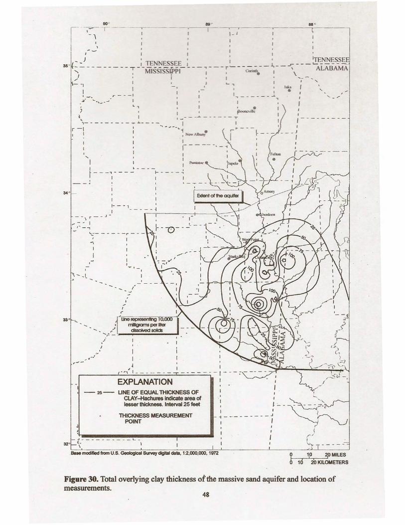
Figure 30. Total overlying clay thickness of the massive sand aquifer and location ofmeasurements.
48
..•... 89 --,---------,,------.- -I
,, ' i
350 } TENNESSEE ' ' !E..:"l;!~S_S£~- - - - - - - - - T -'- - - - -.r;.. - - !.. - - , - - - r ~ - -L~ - - 1,- - ~ ALABAMA!
<, ,MISSISS!(,PI;, 8' \ I
-I . , , " '- - _ 'I/~, '--, , ", I•••.••I I I' 0;) '- -II _.. r - - -I ,. ..J. , "- I.If ~.,_.~ I " 1
, L , , 8 I/ ,~ -'-_. ;'Ic f ~- \- ~ .1._ _ _ _ I
r~1 - - I "'-~--'";
, ' , ew A11=ly8
r ': :____ I-~1_ - J - - -'~ - ~ - - ~ - - - - ~ - ~ - .
ti , ;
34° . I . I I
, .' i- l- - - 1 '
- ------1 I_' - I-- r--J I -
I \ --,- - - I I
.> -., 1_ - -.- - - -- - .• ----;---"'>-T""""'~------r---- ~-,
I
\
!- II
,I-'- ,
t----r= ~ J
, ,I ',
FUltOJl~- - - ~- - - -@ ,,,
,- -"1
-,
I-' .L __ I
/-...,
I I I I
r- 1--: Una represenl1ng10,
33 0 - ,/ mU~ms per Iller- , .•... :. cHssc»Ied solICb
- ••.•. -' r- '=--------......_,::('__ --; I,.; ,
II
- ~ , 'f ." ,- - - -- - - - ..• - - - - - - - t ~ - - - - - - - - -./ \ , .,
I - ,\
-25-
EXPLANATIONLINE OF EaUAL THICKNESS OFCLAY-Interval25 feet
THICKNESS MEASUREMENTPOINT
~~ ~ ...........•........•••_J L_
~o \ ,
_Basemodified from u.s. Geologic:al Survey digtal data, 1:2,000,000, -1972 ~ 1,0 2,0 MILES10 2'0 KILOMETERS
Figure 31. Total overlying clay thickness of the Lower Cretaceous aquifer and location ofmeasurements,
49

90° 69°
I, SHELBY
~- - .,
FAYETTE HARDEMAN McNAIRY ~ HARD!N WAYNE
TENNESSEE- - - - - - - - - ~ - -MrSSISS}j>PI- - - ~ - - -DESOTO I BENTON;
;--4 1 .- _ • • __ I
~ .L/~~"~.'~;"._..-_.J' ;
() .: ~--I
> ) TATE
!~ ;.•... -- - ------------. --- -- .•. - -~--------., ':----1 --'..- - ~~
!,
MARSHALLTIPPAH
;TENNESSE1"'""---0,...-------, ALABAMA\ii"""\LAUDERDALE
, I -." ",
"
COLBERT, .t _
,
UNION@
New Albany FRANKLIN
PANOLA LAFAYETTE
~?~ I I I
~ ~- - - - -. -;--,. - - - - - - - -~'-- - - - - - - - -:.- -_. - - - - _. - j: ~ I I
i
PONTOTOC
Pontotoc-
YALOBUSHA
TALLAHATCHIE CALHOUN,,- - -- - --I : -:
t------,---
CARROLL OKTIBBEHA
CHOCTAW
ATALLA
,;'T!-'-- -:--
,- - - -; ;I •. ,,
,NOXUBEE
. ,__ L. • _ .•... _,
HOLMESWINSTON
,I":
--.,!:...., - --
~ . ~ .•, • t - - - - - - --, .. ,
,Yf'(ZOO LEAKE
NESHOBA
'--,MADISON .',
" , ,f··· .....•·, I ~---
.' I ,
,;' \}'_.'.
" .... ,r.·',.'
~iJ:--\_-!,-~,,'---;~~f.:~ .
~",~,
: "'"DEROME !__~_:,~.-.-.- -.-._.- _._._._; ~~; ,CHOCTAW ;,'\.t--.------- ...--~"".,.-.-IIII!Il!lJ!!l!II!II!,.... CLARKE' ,.,.' MORENGO, ,
- - - .. - - - - - - - - - - - - - - - - - - _. _. - -'-.32° ~, SIMPSON;
Base modified from U.S. Geological Survey digital data, 1:2,000,000, 1972
EXPLANATIONRECHARGE IN OUTCROP AREA
o DISCHARGE IN OUTCROP AREA
'~; _._. - 'LARK' _._.~ 1,0 2,0MI LESo 10 2'0 KILOMETERS
Figure 52. Areas of simulated 1995 recharge and discharge in aquifer outcrops,73

This page intentionally left blank.
Related Documents