Appendix II: STATA Preliminary - World Banksiteresources.worldbank.org/PGLP/Resources/ap2.pdfDisplays each command and results or feedback generated by the command Stata Command Lists

Appendix II: STATA Preliminary

STATA is a statistical software package that offers a large number of statistical and econometric estimation procedures. With STATA we can easily manage data and apply standard statistical and econometric methods such as regression analysis and limited dependent variable analysis to cross-sectional or longitudinal data.

11.. GGeettttiinngg SSttaarrttee dd

1.1. Starting STATA

Start a STATA session by double -clicking on the STATA icon in your desktop. The

STATA computing environment comprises four main windows. The size and shape of these

windows may be moved about on the screen. Their general look and description are shown

below:

Review Stata Results

Lists previous commands entered in the STATA Command window during current session

Variables

Displays each command and results or feedback generated by the

command

Stata Command

Lists all variables of the currently open dataset

STATA commands are entered here. It shows a blinking command prompt

2

It is useful to have the Stata Results window be the largest so you can see a lot of information about your commands and output on the screen. In addition to these windows STATA environment has a menu and a toolbar at the top (to perform STATA operations) and a directory status bar at the bottom (that shows the current directory). You can use menu and toolbar to issue different STATA commands (like opening and saving data files), although most of the time it is more convenient to use the Stata Command window to perform those tasks. If you are creating a log file (see below for more details), the contents can also be displayed on the screen; this is sometimes useful if one needs to back up to see earlier results from the current session.

1.2. Opening a Dataset

You open a STATA dataset by entering following command in the Stata Command window:

use hh

(or possibly use c:\intropov\data\hh, depending on where STATA has opened up; see below for more details). STATA responds by displaying the following in the Stata Results window:

. use hh

.

The first line repeats the command you enter and the second line with no error message

implies that the command has been executed successfully. From now on, we will show only the Stata Results window to demonstrate STATA commands. The following points should be noted:

• STATA assumes the file to be in STATA format with an extension .dta. So, typing hh is the same as typing hh.dta.

• We can only have one data set open at a time in STATA. So if we open another data set ind.dta, we will be replacing hh.dta with ind.dta.

• The above command assumes that the file hh.dta is in the current directory (shown by the directory status bar at the bottom). If that is not the case then you can do one of the following two things (assuming current directory is c:\stata\data and the file hh.dta is in c:\intropov):

•

§ Type the full path of the data file:

. use c:\intropov\hh

3

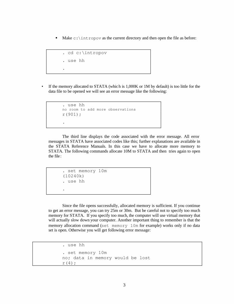
§ Make c:\intropov as the current directory and then open the file as before:

. cd c:\intropov

. use hh

.

• If the memory allocated to STATA (which is 1,000K or 1M by default) is too little for the data file to be opened we will see an error message like the following:

. use hh no room to add more observations r(901);

.

The third line displays the code associated with the error message. All error

messages in STATA have associated codes like this; further explanations are available in the STATA Reference Manuals. In this case we have to allocate more memory to STATA. The following commands allocate 10M to STATA and then tries again to open the file :

. set memory 10m (10240k) . use hh

.

Since the file opens successfully, allocated memory is sufficient. If you continue to get an error message, you can try 25m or 30m. But be careful not to specify too much memory for STATA. If you specify too much, the computer will use virtual memory that will actually slow down your computer. Another important thing to remember is that the memory allocation command (set memory 10m for example) works only if no data set is open. Otherwise you will get following error message:

. use hh

. set memory 10m no; data in memory would be lost r(4);

4

You can clear the memory using one of the two commands: clear or

drop _all. The following demonstration shows the first command:

. use hh

. set memory 10m no; data in memory would be lost r(4);

. clear

. set memory 10m

.

1.3 . Saving a Data set

If you make changes in an open STATA data file and want to save those changes, you can do that by using the STATA save command. For example, the following command saves the hh.dta file:

. save hh, replace

file hh.dta saved

You can optionally omit the filename here (just save, replace is good enough). If you do not use the replace option STATA does not save the data but issues the following error message:

. save hh file hh.dta already exists r(602);

The replace option unambiguously tells STATA to overwrite the pre-existing original version with the new version. If you do NOT want to lose the original version, you have to specify a different filename in the save command:

. save hh1

file hh1.dta saved

5

Notice that there is no replace option here. However, if a file named hh1.dta already exists then you have to either use the replace option or use a new filename.

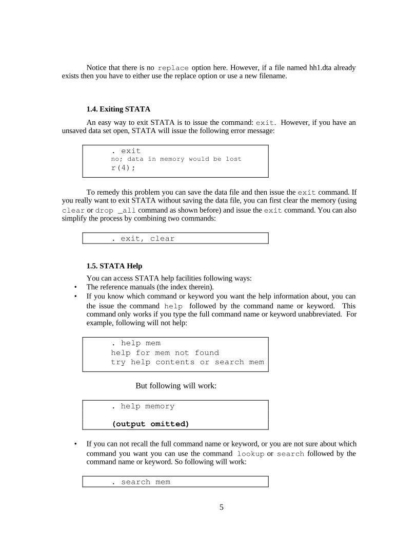
1.4. Exiting STATA

An easy way to exit STATA is to issue the command: exit. However, if you have an unsaved data set open, STATA will issue the following error message:

. exit no; data in memory would be lost r(4);

To remedy this problem you can save the data file and then issue the exit command. If

you really want to exit STATA without saving the data file, you can first clear the memory (using clear or drop _all command as shown before) and issue the exit command. You can also simplify the process by combining two commands:

. exit, clear

1.5. STATA Help

You can access STATA help facilities following ways: • The reference manuals (the index therein). • If you know which command or keyword you want the help information about, you can

the issue the command help followed by the command name or keyword. This command only works if you type the full command name or keyword unabbreviated. For example, following will not help:

. help mem help for mem not found try help contents or search mem

But following will work:

. help memory (output omitted)

• If you can not recall the full command name or keyword, or you are not sure about which

command you want you can use the command lookup or search followed by the command name or keyword. So following will work:

. search mem

6

(output omitted)

This command will list all commands associated with this keyword and display a brief description of each of those commands. Then you can pick what you think is relevant and use “help” to obtain the specific reference.

• The STATA website (http://www.stata.com) has excellent help facilities, for example, Online Tutorial, Frequently Asked Questions (FAQ), etc.

1.6. Notes on STATA Commands

Here are some general comments about STATA commands:

• STATA commands are typed in lower case. • All names, including commands or variable names, can be abbreviated as long as there is no

ambiguity. So describe, des or simply d do the same job as there is no confusion.

• In addition to typing, some keystrokes can be used to represent a few STATA commands or sequences. The most important of them are the Page-Up and Page-Down keys. To display the previous command in Stata Command window, you can press Page-Up key. You can keep doing that until the first command of the session appears. Similarly, the Page-Down key displays the command that follows the currently displayed command in the Stata Command window.

22.. WWoorrkkiinngg wwiitthh ddaattaa ff iilleess:: llooookkiinngg aatt tthhee ccoonntteenntt From now on, we will mostly list the command(s) and not the results, to save

space. To go through this exercise open the hh.dta file, as we will use examples extensively from this data file.

2.1. Listing the variables

To see all variables in the data set, use the describe command (fully or abbreviated):

. describe

This command provides you with information about the data set (name, size,

number of observations) and lists all variables (name, storage format, display format, label).

To see just one variable or list of variables use the describe command

followed by the variable name(s):

7

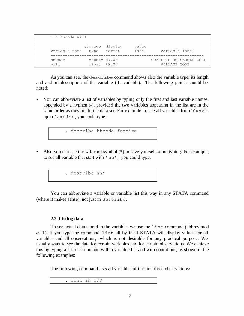
. d hhcode vill storage display value variable name type format label variable label ---------------------------------------------------------------- hhcode double %7.0f COMPLETE HOUSEHOLD CODE vill float %2.0f VILLAGE CODE

As you can see, the describe command shows also the variable type, its length

and a short description of the variable (if available). The following points should be noted:

• You can abbreviate a list of variables by typing only the first and last variable names,

appended by a hyphen (-), provided the two variables appearing in the list are in the same order as they are in the data set. For example, to see all variables from hhcode up to famsize, you could type:

. describe hhcode-famsize

• Also you can use the wildcard symbol (*) to save yourself some typing. For example, to see all variable that start with "hh", you could type:

. describe hh*

You can abbreviate a variable or variable list this way in any STATA command (where it makes sense), not just in describe.

2.2. Listing data

To see actual data stored in the variables we use the list command (abbreviated as l). If you type the command list all by itself STATA will display values for all variables and all observations, which is not desirable for any practical purpose. We usually want to see the data for certain variables and for certain observations. We achieve this by typing a list command with a variable list and with conditions, as shown in the following examples:

The following command lists all variables of the first three observations:

. list in 1/3

8

Here STATA displays all observations starting from observation 1 and ending

with observation 3. STATA can also display data as a spreadsheet. There are two icons in the toolbar called Data Editor and Data Browser (fourth and third from right). By clicking one, a new window will pop up and the data will be displayed as a table, with observations as rows and variables as columns. Data Browser will only display the data, whereas you can edit data with Data Editor. The commands edit and browse will also open the spreadsheet window.

The following command lists household size and head's education for households

headed by a female who is younger than 45:

. list hhid hhsize headedu if headsex==2 & headage<45

The above statement uses two relational operators (== and <) and one logical operator (&). Relational operators impose a condition on one variable, while logical operators combine two or more relational operators. The following list shows the relational and logical operators that are used in STATA:

Relational operators Logical operators

> (greater than) ~ (not)

< (less than) | (or)

== (equal) & (and)

>= (greater than or equal)

>= (less than or equal)

!= or ~= (not equal)

You can use relational and logical operators in any STATA command (where it makes sense), not just in the list command.

2.3. Summarizing data

The command summarize (abbreviated sum) calculates and displays a variety of summary statistics, for example means and standard deviations. If no variable is specified, summary statistics are calculated for all variables in the data set. The following command summarizes the household size and education of the household head:

. sum famsize educhead

9

Any observation that has a missing value for the variable(s) being summarized is

excluded from this calculation by STATA (missing values are discussed later). With no option, summarize provides the mean, standard deviation, minimum and maximum for each variable. If we want to know the median and percentiles of a variable, we need to add the detail option (abbreviated d):

. sum famsize educhead, d

STATA allows the use of weights. The weight option is useful if the sampling

probability of one observation is different from another. In most household surveys, the sampling frame is stratified, where the first primary sampling units (often villages) are sampled, and conditional on the selection of primary sampling unit, secondary sampling units (often households) are drawn. Household surveys generally provide weights to correct for the sampling design differences and sometimes data collection problems. The implementation in STATA is straightforward:

. sum famsize educhead [pw=weight]

Here the variable weight has the information on the weight to be given to each observation and pw is a STATA option to incorporate the weight into the calculation. We will discuss the use of weights further in chapter exercises that follow this exercise.

For variables that are strings, summarize will not be able to give any

descriptive statistics except that the number of observations is zero. Also, for variables that are categorical, it can be difficult to interpret the output of the summarize command. In both cases, a full tabulation may be more meaningful, which we will discuss next.

Many times we want to see summary statistics by group of certain variables, not just for the whole data set. Say in the above example, we want to see mean of family size and education of household head by the gender of household head. Of course, we can use a condition in the sum command (for example, sum famsize educhead if sexhead==1 [pw=weight]), but this is not convenient if the variability of the group variable increases (for example, the variable region). In those cases, we use by option of STATA which makes life much simpler. For example, we want to see summary statistics of family size and education of household head for each region. Before we use STATA by option we must make sure that data is sorted by the group variable. You can check this by issuing describe command after opening each file. describe command, after listing all the variables, informs if the data set is sorted by any variable(s). If there is no sorting information listed or the data set is sorted by variable(s)

10

that is (are) different from what you want it to be, you can issue a sort command and then save the data set in this form. Following commands sort the data set by region and show summary statistics of family size and education of household head by region:

. sort region . by region: sum famsize educhead [pw=weight]

2.4. Frequency distributions (tabulations)

We often need frequency distributions and cross tabulations. We use the tabulate (abbreviated tab) command to do this. The following command gives the regional distribution of the households:

. tab region

The following command gives the gender distribution of household heads in region 1:

. tab sexhead if region==1

In passing, note the use of the == sign here. It indicates that if the regional variable is identically equal to 1, then do the tabulation.

We can use the tabulate command to make a two-way distribution. For

example, we would like to check whether there is any gender bias in the education of household heads. We use the following command:

. tab educhead sexhead

To see percentages by row or columns we can add options to the tabulate

command:

. tab region sexhead, col row

11

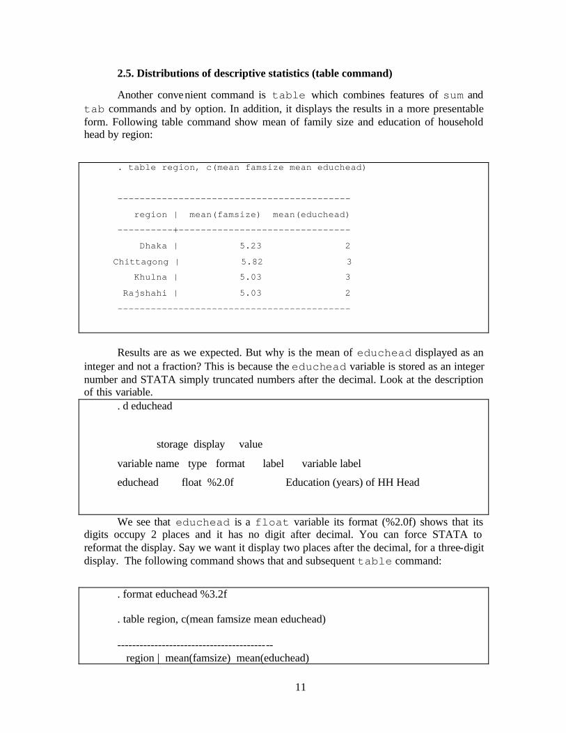
2.5. Distributions of descriptive statistics (table command)

Another convenient command is table which combines features of sum and tab commands and by option. In addition, it displays the results in a more presentable form. Following table command show mean of family size and education of household head by region:

. table region, c(mean famsize mean educhead)

------------------------------------------

region | mean(famsize) mean(educhead)

----------+-------------------------------

Dhaka | 5.23 2

Chittagong | 5.82 3

Khulna | 5.03 3

Rajshahi | 5.03 2

------------------------------------------

Results are as we expected. But why is the mean of educhead displayed as an

integer and not a fraction? This is because the educhead variable is stored as an integer number and STATA simply truncated numbers after the decimal. Look at the description of this variable.

. d educhead

storage display value

variable name type format label variable label

educhead float %2.0f Education (years) of HH Head

We see that educhead is a float variable its format (%2.0f) shows that its digits occupy 2 places and it has no digit after decimal. You can force STATA to reformat the display. Say we want it display two places after the decimal, for a three-digit display. The following command shows that and subsequent table command:

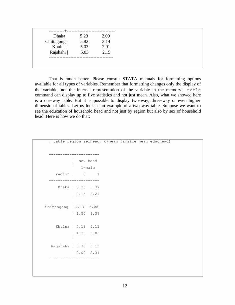
. format educhead %3.2f . table region, c(mean famsize mean educhead) ------------------------------------------ region | mean(famsize) mean(educhead)

12

----------+------------------------------- Dhaka | 5.23 2.09

Chittagong | 5.82 3.14 Khulna | 5.03 2.91 Rajshahi | 5.03 2.15 ------------------------------------------

That is much better. Please consult STATA manuals for formatting options available for all types of variables. Remember that formatting changes only the display of the variable, not the internal representation of the variable in the memory. table command can display up to five statistics and not just mean. Also, what we showed here is a one-way table. But it is possible to display two-way, three-way or even higher dimensional tables. Let us look at an example of a two-way table. Suppose we want to see the education of household head and not just by region but also by sex of household head. Here is how we do that:

. table region sexhead, c(mean famsize mean educhead)

----------------------

| sex head

| 1=male

region | 0 1

----------+-----------

Dhaka | 3.36 5.37

| 0.18 2.24

|

Chittagong | 4.17 6.08

| 1.50 3.39

|

Khulna | 4.18 5.11

| 1.36 3.05

|

Rajshahi | 3.70 5.13

| 0.00 2.31

----------------------

13

2.5. Missing Values in STATA

In STATA, a missing value is represented by a dot (.). A missing value is considered larger than any number. The summarize command ignores the observations with missing values and the tabulate command does the same, unless forced include missing values.

2.6. Counting observations

We use count command to count the number of observations in the data set:

. count 519 .

The count command can be used with conditions. The following command

gives the number of households whose head is older than 50:

. count if agehead>50 161 .

33.. WWoorrkkiinngg wwiitthh ddaattaa ff iilleess:: cchhaanngg iinngg ddaattaa sseett

3.1. Generating new variables

In STATA the command generate (abbreviated gen) creates new variables, while the command replace changes the values of an existing variable. The following commands create a new variable called oldhead, then set its value to 1 if the household head is older than 32 years and to 0 otherwise:

. gen oldhead=1 if agehead>32 (90 missing values generated)

. replace oldhead=0 if agehead<=32 (90 real changes made)

What happens here is, for each observation, the generate command checks the

condition (whether household head is older than 32) and sets the value of the variable

14

oldhead to 1 for that observation if the condition is true, and to missing value otherwise. The replace command works in a similar fashion (however, the condition is reversed here and oldhead gets 0 if the condition is met). After the generate command STATA informs us that 90 observations failed to meet the condition and after the replace command STATA informs us that those 90 observations have got new values (0 in this case). The following points should be made:

• STATA variable names cannot be longer than 8 letters. So generate/replace

commands must conform to this. • If a generate or replace command is issued without any conditions, that

command applies to all observations in the data file. • While using the generate command, care should be taken to handle missing values

properly. • The right hand side of the = sign in the generate or replace commands can be

any expression involving variable names, not just a value. • The command replace does not have to always follow the generate command.

The replace command can be used to change the values of any existing variable, independently of generate command.

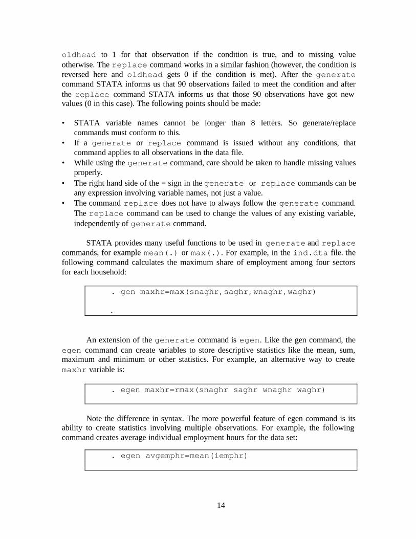
STATA provides many useful functions to be used in generate and replace

commands, for example mean(.) or max(.). For example, in the ind.dta file. the following command calculates the maximum share of employment among four sectors for each household:

. gen maxhr=max(snaghr,saghr,wnaghr,waghr) .

An extension of the generate command is egen. Like the gen command, the

egen command can create variables to store descriptive statistics like the mean, sum, maximum and minimum or other statistics. For example, an alternative way to create maxhr variable is:

. egen maxhr=rmax(snaghr saghr wnaghr waghr)

Note the difference in syntax. The more powerful feature of egen command is its

ability to create statistics involving multiple observations. For example, the following command creates average individual employment hours for the data set:

. egen avgemphr=mean(iemphr)

15

All observations in the data set get the same value for avgemphr. The following command creates the same statistics, this time for males and females:

. egen avghrmf=mean(iemphr), by(sex)

Here observations for males get the value that is average of male employment

hours, while observations for females get the equivalent for female employment hours.

3.2. Labeling

3.2.1. Labeling variables You can attach labels to variables to give a description to them. For example, the

variable oldhead does not have any label now. You can attach a label to this variable by typing:

. label variable oldhead "HH Head is over 32"

In the label command, variable can be shortened to var. Now to see the

new label, type:

. des oldhead

3.2.2. Labeling Data There are other types of labels we can create. To attach a label to the entire data

set, which appears at the top of our describe list:

. label data “Bangladesh HH Survey 1998/99”

To see this label, type:

. des 3.2.3. Labeling Values of variables Variables that are categorical, like those in sexhead (1=male, 0=female), can

have labels that help one to remember what the categories are. For example, if we tabulate the variable sexhead we see only 0 and 1 values:

16

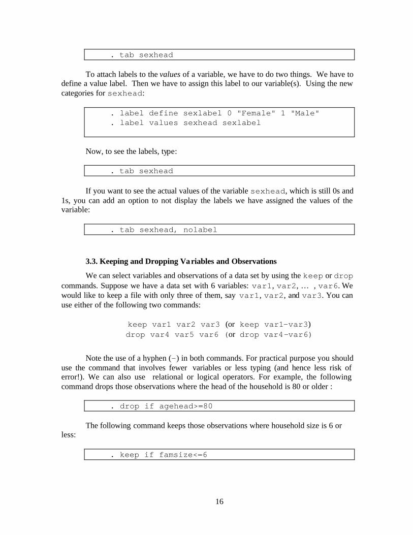
. tab sexhead To attach labels to the values of a variable, we have to do two things. We have to

define a value label. Then we have to assign this label to our variable(s). Using the new categories for sexhead:

. label define sexlabel 0 "Female" 1 "Male" . label values sexhead sexlabel

Now, to see the labels, type:

. tab sexhead If you want to see the actual values of the variable sexhead, which is still 0s and

1s, you can add an option to not display the labels we have assigned the values of the variable:

. tab sexhead, nolabel

3.3. Keeping and Dropping Variables and Observations

We can select variables and observations of a data set by using the keep or drop commands. Suppose we have a data set with 6 variables: var1, var2, … , var6. We would like to keep a file with only three of them, say var1, var2, and var3. You can use either of the following two commands:

keep var1 var2 var3 (or keep var1-var3) drop var4 var5 var6 (or drop var4-var6)

Note the use of a hyphen (-) in both commands. For practical purpose you should

use the command that involves fewer variables or less typing (and hence less risk of error!). We can also use relational or logical operators. For example, the following command drops those observations where the head of the household is 80 or older :

. drop if agehead>=80

The following command keeps those observations where household size is 6 or

less:

. keep if famsize<=6

17

The above two commands drop or keep all variables based on the conditions. You cannot include a variable list in a drop or keep command that also uses conditions. For example, the following command will fail:

. keep hhcode famsize if famsize<=6 invalid sytax r(198);

You have use two commands to do the job:

. keep if famsize<=6

. keep hhcode famsize

You can also use the keyword in a drop or keep command. For example, to drop the first 20 observations:

. drop in 1/20

3.4. Producing Graphs

STATA is quite good at producing basic graphs, although considerable experimentation may be needed to produce really beautiful graphs. The following command shows the distribution of the age of the household head in a bar graph:

. graph agehead

Whether you use a categorical variable or a continuous variable, say income, does

not make a difference to STATA: the default is 5 bars (“bins”). The number of bars may be increased, up to a maximum of 50, by adding the option bin(#).

. graph agehead, bin(12) In order to save the graph we would add the option saving(filename). You

can also provide titles. For a scatter plot of two variables, type the following command: graph headedu headage, t1(education by age) saving(eduage,

replace) ylab xlab s(.)

3.5. Combining Data sets

3.5.1. Merging data sets

18

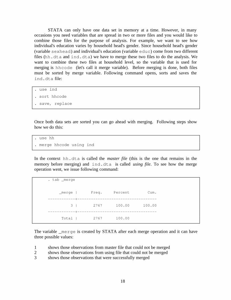
STATA can only have one data set in memory at a time. However, in many occasions you need variables that are spread in two or more files and you would like to combine those files for the purpose of analysis. For example, we want to see how individual's education varies by household head's gender. Since household head's gender (variable sexhead) and individual's education (variable educ) come from two different files (hh.dta and ind.dta) we have to merge these two files to do the analysis. We want to combine these two files at household level, so the variable that is used for merging is hhcode (let's call it merge variable). Before merging is done, both files must be sorted by merge variable. Following command opens, sorts and saves the ind.dta file:

. use ind

. sort hhcode

. save, replace

Once both data sets are sorted you can go ahead with merging. Following steps show how we do this: . use hh . merge hhcode using ind

In the context hh.dta is called the master file (this is the one that remains in the memory before merging) and ind.dta is called using file. To see how the merge operation went, we issue following command:

. tab _merge

_merge | Freq. Percent Cum.

------------+-----------------------------------

3 | 2767 100.00 100.00

------------+-----------------------------------

Total | 2767 100.00

The variable _merge is created by STATA after each merge operation and it can have three possible values: 1 shows those observations from master file that could not be merged 2 shows those observations from using file that could not be merged 3 shows those observations that were successfully merged

19

Total number of observations in the resulting data set is the sum of these three _merge frequencies. Possible candidate for _merge=1 is an observation in hh.dta file that has a hhcode values which cannot be found in ind.dta file. Similarly if the ind.dta file has a hhcode that is not found in the hh.dta file that observation will appear with _merge=2. In the above example, however, each household in hh.dta file has an exact match in the ind.dta file and that is why we got _merge=3 and not 1's or 2's. If you keep only the matched observations, you can do that by this command: keep if _merge==3. Once we have merged the data sets we can go ahead with our analysis:

. sort sexhead

. by sexhead: sum educ

-> sexhead = 0

Variable | Obs Mean Std. Dev. Min Max

-------------+-------------------------------------------------

educ | 179 2.329609 3.424591 0 14

________________________________________________________________

-> sexhead = 1

Variable | Obs Mean Std. Dev. Min Max

-------------+---------------------------------------------------

educ | 2588 2.340417 3.324081 0 16

The result shows that there is not much difference in education by the gender of household head.

Notice that in order to show the results by sexhead variable, we have to sort the data by that variable, otherwise we will get an error message. The preference of master and using data is not important and a matter of convenience.

3.5.2. Appending data sets Consider what would happen in the above merging scenario if we have _merge=1 and 2 only but no 3s. This can happen if individual data (ind.dta) come from households that are completely different from the households in hh.dta. In this case resulting number of observations after merging is the sum of observations in the two files (observations with _merge=1 + observations with _merge=2). STATA in this case would actually append the two data sets; however variables that are only included in one file will have missing values for all observation from the other file.. Although this is not what we intend in the above example, appending is necessary when we need to combine two data sets that have same (or almost same) variables but are mutually exclusive. For example, assume we have four regional version of hh.dta file: hhdhak.dta (has households

20

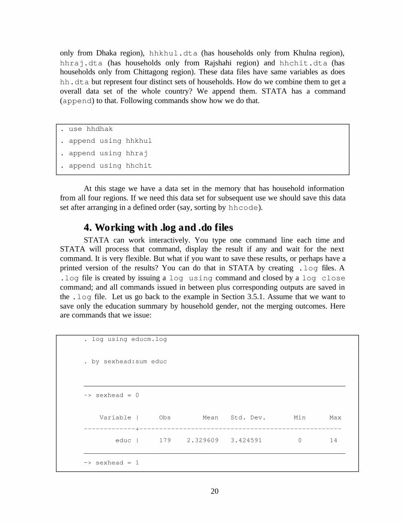
only from Dhaka region), hhkhul.dta (has households only from Khulna region), hhraj.dta (has households only from Rajshahi region) and hhchit.dta (has households only from Chittagong region). These data files have same variables as does hh.dta but represent four distinct sets of households. How do we combine them to get a overall data set of the whole country? We append them. STATA has a command (append) to that. Following commands show how we do that.

. use hhdhak . append using hhkhul

. append using hhraj

. append using hhchit

At this stage we have a data set in the memory that has household information

from all four regions. If we need this data set for subsequent use we should save this data set after arranging in a defined order (say, sorting by hhcode).

44.. WWoorrkkiinngg wwiitthh ..lloogg aanndd ..ddoo ff iilleess STATA can work interactively. You type one command line each time and

STATA will process that command, display the result if any and wait for the next command. It is very flexible. But what if you want to save these results, or perhaps have a printed version of the results? You can do that in STATA by creating .log files. A .log file is created by issuing a log using command and closed by a log close command; and all commands issued in between plus corresponding outputs are saved in the .log file. Let us go back to the example in Section 3.5.1. Assume that we want to save only the education summary by household gender, not the merging outcomes. Here are commands that we issue:

. log using educm.log

. by sexhead:sum educ

__________________________________________________________________

-> sexhead = 0

Variable | Obs Mean Std. Dev. Min Max

-------------+---------------------------------------------------

educ | 179 2.329609 3.424591 0 14

__________________________________________________________________

-> sexhead = 1

21

Variable | Obs Mean Std. Dev. Min Max

-------------+---------------------------------------------------

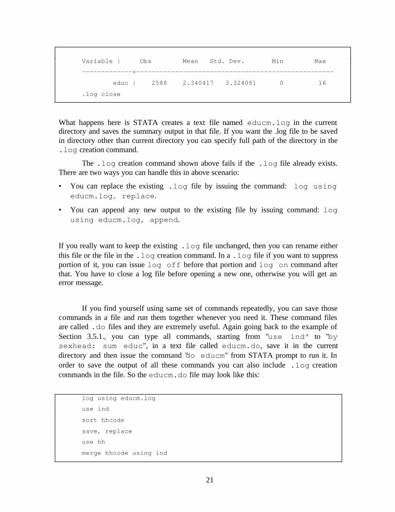
educ | 2588 2.340417 3.324081 0 16

.log close

What happens here is STATA creates a text file named educm.log in the current directory and saves the summary output in that file. If you want the .log file to be saved in directory other than current directory you can specify full path of the directory in the .log creation command.

The .log creation command shown above fails if the .log file already exists. There are two ways you can handle this in above scenario:

• You can replace the existing .log file by issuing the command: log using educm.log, replace.

• You can append any new output to the existing file by issuing command: log using educm.log, append.

If you really want to keep the existing .log file unchanged, then you can rename either this file or the file in the .log creation command. In a .log file if you want to suppress portion of it, you can issue log off before that portion and log on command after that. You have to close a log file before opening a new one, otherwise you will get an error message.

If you find yourself using same set of commands repeatedly, you can save those commands in a file and run them together whenever you need it. These command files are called .do files and they are extremely useful. Again going back to the example of Section 3.5.1., you can type all commands, starting from "use ind" to "by sexhead: sum educ", in a text file called educm.do, save it in the current directory and then issue the command "do educm" from STATA prompt to run it. In order to save the output of all these commands you can also include .log creation commands in the file. So the educm.do file may look like this:

log using educm.log

use ind

sort hhcode

save, replace

use hh

merge hhcode using ind

22

tab _merge sort sexhead

by sexhead:sum educ

log close

The main advantage of using .do file instead of typing commands line by line is repeatability. Usually if it takes quite some steps to obtain the desired output, you should edit a .do file because you may need to do it tens of times.

There are certain commands that are useful in a .do file. We will discuss them from the following sample .do file:

*This is a STATA comment which is not executed

/*****This is a do file that shows some very useful

commands used in do files. In addition, it creates a

log file and uses some basic STATA commands ***/

#delimit ;

set more 1;

drop _all;

cap log close;

log using c:\intropov\logfiles\try1.log, replace;

use “c:\intropov\data\hh.dta”;

describe;

list in 1/3;

list hhid hhsize headedu if headsex==2 & headage<45;

summarize hhsize;

summarize hhsize, detail; sum hhsize headedu [pw=weight], d;

tabulate headsex;

tabulate headedu headsex, col row chi;

tabulate headedu, summarize(headage);

label define sexlabel 1 “MALE” 2 “FEMALE”;

23

label values headsex sexlabel;

tabulate headsex;

label variable headsex “Head Gender”;

use “c:\intropov\data\hh.dta”;

sort hhid;

save temp, replace;

use “c:\intropov\data\consume.dta”, clear;

sort hhid ;

merge hhid using temp;

tabulate _merge;

keep if _merge==3;

log close;

exit; The first line in the file is a comment. STATA treats any line that starts with an

asterisk (*) as a comment and ignores it. You can write multi- line comment by using forward slash and asterisk (/*) as the start of the comment and end the comment by asterisk and forward slash (*/). Comments are very useful for documentation purpose and you should include at least following information in the comment of a do file: general purpose of the do file, and last modification time and date. You can include comment anywhere in the do file, not just at the beginning.

#delimit ; By default STATA assumes that each command is ended by the

carriage return (ENTER key press). If, however, a command is too long to be fit in one line you can spread it over more than one line. You do that by letting STATA know what the command delimiter would be. The command in the example says that a command is ended by a semicolon (;). Every command following the delimit command has to end with a ; until the file ends or another #delimit cr command appears which makes carriage return again the command delimiter. Although for this particular .do file we don't need to use the #delimit command it is done to explain the command.

set more 1 STATA usually displays results one screenful at a time, and waits

for the user to press any key. But this would soon become a pain if after starting a .do file to run you have to press a key every time

24

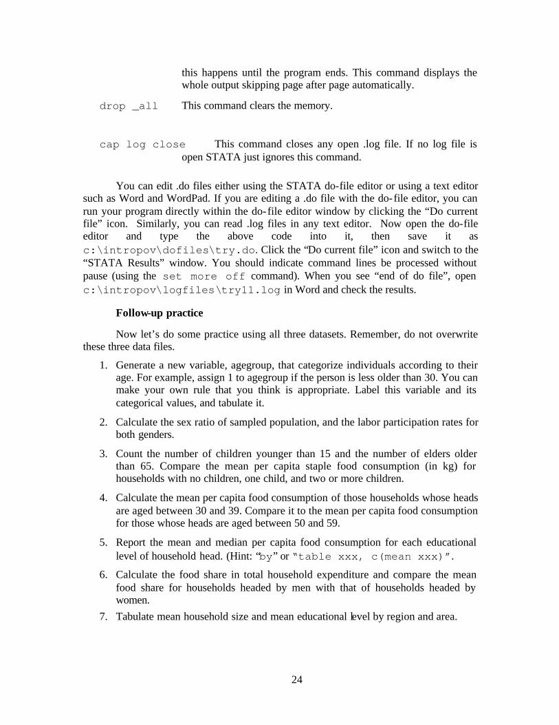
this happens until the program ends. This command displays the whole output skipping page after page automatically.

drop _all This command clears the memory.

cap log close This command closes any open .log file. If no log file is open STATA just ignores this command.

You can edit .do files either using the STATA do-file editor or using a text editor

such as Word and WordPad. If you are editing a .do file with the do-file editor, you can run your program directly within the do-file editor window by clicking the “Do current file” icon. Similarly, you can read .log files in any text editor. Now open the do-file editor and type the above code into it, then save it as c:\intropov\dofiles\try.do. Click the “Do current file” icon and switch to the “STATA Results” window. You should indicate command lines be processed without pause (using the set more off command). When you see “end of do file”, open c:\intropov\logfiles\try11.log in Word and check the results.

Follow-up practice

Now let’s do some practice using all three datasets. Remember, do not overwrite these three data files.

1. Generate a new variable, agegroup, that categorize individuals according to their age. For example, assign 1 to agegroup if the person is less older than 30. You can make your own rule that you think is appropriate. Label this variable and its categorical values, and tabulate it.

2. Calculate the sex ratio of sampled population, and the labor participation rates for both genders.

3. Count the number of children younger than 15 and the number of elders older than 65. Compare the mean per capita staple food consumption (in kg) for households with no children, one child, and two or more children.

4. Calculate the mean per capita food consumption of those households whose heads are aged between 30 and 39. Compare it to the mean per capita food consumption for those whose heads are aged between 50 and 59.

5. Report the mean and median per capita food consumption for each educational level of household head. (Hint: “by” or “table xxx, c(mean xxx)”.

6. Calculate the food share in total household expenditure and compare the mean food share for households headed by men with that of households headed by women.

7. Tabulate mean household size and mean educational level by region and area.