APPENDIX C ESTIMATES OF SAMPLING ERRORS Mahir Ulusoy and Alfredo Aliaga The estimates from a sample survey are affected by two types of errors--nonsampling and sampling. Nonsampling errors result from mistakes made in implementing data collection and data processing, such as failure to locate and interview the correct household, misunderstanding of the questions on the part of either the interviewer or the respondent, and data entry errors. Although numerous efforts were made to minimise this type of error during the implementation of the TDHS, nonsampling errors are impossible to avoid and difficult to evaluate statistically. Sampling errors, on the other hand, can be evaluated statistically. The sample of women selected in the TDHS is only one of many samples that could have been selected from the same population, using the same design and expected size. Each of these samples would yield results that would differ somewhat from the results of the actual sample selected. The sampling error is a measure of the variability between all possible samples. Although the degree of variability is not known exactly, it can be estimated from the survey results. Sampling error is usually.measured in terms of the standard error for a particular statistic (mean, percentage, etc.), which isthe ratio of the standard deviation to the square root of the sample size. The standard error can be used to calculate confidence intervals within which the true value for the population can reasonably be assumed to fall. For example, for any given statistic calculated from a sample survey, the value of that statistic will fall within a range of plus or minus two times the standard error of that statistic in 95 percent of all possible samples of identical size and design. If the sample of women had been selected as a simple random sample, it would have been possible to use straightforward formulas for calculating sampling errors. However, the TDHS sample is the result of a three-stage stratified design, and, consequently, it was necessary to use more complex formulas. The computer package CLUSTERS, developed by the International Statistical Institute for the World Fertility Survey, was used to compute the sampling errors for 42 variables with the proper statistical methodology. The CLUSTERS package treats any percentage or average as a ratio estimate, r = y/x, where y represents the total sample value for variable y, and x represents the total number of cases in the group or subgroup under consideration. The variance of r is computed using the formula given below, with the standard error being the square root of the variance, var(r) = 1-f mh 2 Zh x 2 mh-----i i=1 k in which Zhi = Yhi-r.Xhi , and Zh = yh-r.xh 143

Welcome message from author
This document is posted to help you gain knowledge. Please leave a comment to let me know what you think about it! Share it to your friends and learn new things together.
Transcript
APPENDIX C
ESTIMATES OF SAMPLING ERRORS
Mahir Ulusoy and Alfredo Aliaga
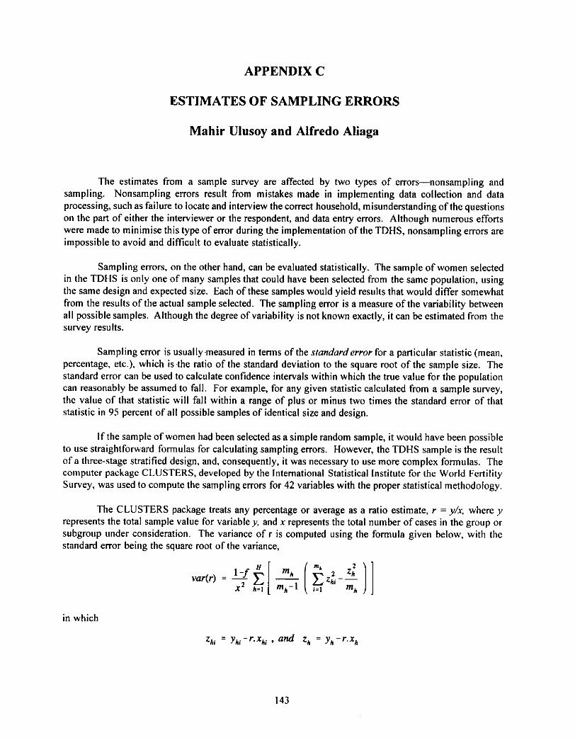
The estimates from a sample survey are affected by two types of errors--nonsampling and sampling. Nonsampling errors result from mistakes made in implementing data collection and data processing, such as failure to locate and interview the correct household, misunderstanding o f the questions on the part of either the interviewer or the respondent, and data entry errors. Although numerous efforts were made to minimise this type of error during the implementation of the TDHS, nonsampling errors are impossible to avoid and difficult to evaluate statistically.
Sampling errors, on the other hand, can be evaluated statistically. The sample o f women selected in the TDHS is only one of many samples that could have been selected from the same population, using the same design and expected size. Each of these samples would yield results that would differ somewhat from the results of the actual sample selected. The sampling error is a measure of the variability between all possible samples. Although the degree of variability is not known exactly, it can be estimated from the survey results.
Sampling error is usually.measured in terms of the standard error for a particular statistic (mean, percentage, etc.), which is the ratio of the standard deviation to the square root of the sample size. The standard error can be used to calculate confidence intervals within which the true value for the population can reasonably be assumed to fall. For example, for any given statistic calculated from a sample survey, the value o f that statistic will fall within a range of plus or minus two times the standard error of that statistic in 95 percent of all possible samples of identical size and design.
If the sample of women had been selected as a simple random sample, it would have been possible to use straightforward formulas for calculating sampling errors. However, the TDHS sample is the result of a three-stage stratified design, and, consequently, it was necessary to use more complex formulas. The computer package CLUSTERS, developed by the International Statistical Institute for the World Fertility Survey, was used to compute the sampling errors for 42 variables with the proper statistical methodology.
The CLUSTERS package treats any percentage or average as a ratio estimate, r = y/x, where y represents the total sample value for variable y, and x represents the total number of cases in the group or subgroup under consideration. The variance of r is computed using the formula given below, with the standard error being the square root of the variance,
var(r) = 1 - f mh 2 Zh
x 2 mh-----i i=1 k
in which
Zhi = Y h i - r . X h i , a n d Z h = y h - r . x h
143

where h II1 h
Yhi xhi
f
represents the stratum that varies from I to H is the total number of standard segments selected in tile la th s t r a t u m
is the sum of the values of variable y in standard segments i in the h th stratum is the sum of the number of cases (women) in standard segments i in the la th stratum is the overall sampling fraction, which is so small that CLUSTERS ignores it.
In addition to tile standard errors, CLUSTERS computes the design effect (DEFT) for each estimate, which is defined as the ratio of the standard error using the given sample design to the standard error that would result if a simple random sample had been used. A DEFT value of 1.0 indicates that the sample design is as efficient as a simple random sample, whereas a value greater than 1.0 indicates the increase in tile sampling error due to the use of a more complex and less statistically efficient design. CLUSTERS also computes the relative error and confidence limits for the estimates.
The results for the 42 variables mentioned, which are those considered to be of primary interest, are presented in this appendix for the country as a whole, for urban and rural areas, for the five regions, and for age groups. The type of statistic (mean or proportion) and the base population for each variable are given in Table C.1. Tables C.2 to C.12 present the value of the statistic (R), its standard error (SE), the number of unweighted (N) and weighted (WN) cases, file design effect (DEFT), the relative standard error (SE/R), and the 95 percent confidence limits (R_+2SE), for each variable.
Additionally, sampling errors were calculated for tile total fertility rote of the last year prior to the survey date and the infant mortality rate for the 5 years preceding the survey, for the national total, and for urban-rural areas. These calculations were undertaken using the Jacknife methodology rather than the CLUSTERS package because of the nature of these two estimates. The Jacknife methodology is based on having replicate values for the estimates and applying the sim pie standard error formulae to these replicates.
Tile TDHS included 478 clusters. Each replication considers all clusters but deletes one cluster at a time for the calculations and then creates pseudoindependent replicates. In total, 478 replications for the infant mortality and total fertility rates create tile pseudoindependent values:
e(.i) = 478 * estimate (all clusters) - 477 * estimate (all minus i ~h)
e estimate (all clusters)
and tile sampling errors for the estimate is given by:
SE (estimate) = {5- (e(.i) - e)-" / (478 * (478-1)) }'/2.
The results of the calcnlations using the Jacknife methodology to estimate sampling errors for the infant mortality rate and tile total fertility rate for the national total, for urban and rural areas, and for the five major regions is shown in Table C.13.
Tile confidence interval (e.g., as calculated for EVBORN) can be interpreted as follows: the overall average from the national sample is 3.041 and the standard error is 0.044. Therefore, to obtain the 95 percent confidence limits, one adds and subtracts twice the standard error to the sample estimate, i.e., 3.041 _+ 0.088. There is a high probability (95 percent) that the true average number of children ever born to all women age 15 to 49 is between 2.954 and 3.128.
Of the 42 variables for which CLUSTERS was used for the estimation of sampling errors, 28 are based on women, and 14 are based on children under age 5. Ill general, the relative standard error for most
144

estimates for the country as a whole is small, except for estimates of very small proportions. There are some differentials in the relative standard error for the estimates of subpopulations such as urban and rural areas. For example, for the variable SECATT (secondary school attendance), the relative standard errors as a percent of the estimated proportion for urban and rural areas are 4.6 percent and 12.5 percent, respectively. The same istrue for SECGRD(proportion of women who completed secondary school) with values of 5 percent and 14.2 percent, for XCUPIL (current use of the pill) with values of 8.1 and 13.6 percent, for XCUIUD (current use of IUD) with values of 3.4 and 8.5 percent, and for XCUPAB (current use of periodic abstinence) with values of 17 percent and 0 percent, for urban and rural areas, respectively for each variable.
O f the 42 variables, 24 were found to have SE/R values of less than 0.03, which means that the SE of those variables is at most 3 percent of the estimate. SE/R values are between 0.031 and 0.059 for 13 variables, and greater than 0.06 for only 5 variables; the maximum value being 16.6 percent. The variables with the highest SE/R ratio are the ones calculated for relatively rare events.
The DEFT value is less than 1.3 for 24 variables; between 1.31 and 1.5 for 13 variables; and greater than 1.51 for only 5 variables. The maximum DEFT value obtained is 1.668. The average of 42 variables is 1.301. The average is 1.213 in urban areas and 1.293 in rural areas for 41 variables (due to the exclusion of the URBAN variable).
145

Table C.I List of selected variables for sampling errors, Turkey 1993
Variable Estimate Base Population
URBAN SECATT SECGRD CURMAR AGEMAR PREGNT NUPRFG NUMISC F, VBORN XEVB XI 'VB40 SURVIV KMETIIO XKMOD XKSOUR XEVUSI" XCUSE XCUPII. X C U I U D
XCUCON XCUWlT XCUSTE XCUPAB XCUMOD XPSOUR XNOMOR XDELAY IDI~AL T H ' A N U MEDEL1 DIARRI DIARR2 ORSTRE MEDTRE RESPI2 RESPI I IICARD BCG I) P 1"3 POL3 Mh:ASLE FULIAM
Urban Proportion Attended secondary or higher Proporlion Graduated secondary or higher Proportion Currently married Proportion Age at marriage Mean Currently pregnant Proporlion Number of pregnancies Mean Number of miscarriages Mean Children ever born Mean Children ever born Mean Children ever born Mean Children surviving Mean Know any method Proportion Know modem method Proporlion Know source of method Proporlion I'ver used any method I'roporlion Currently using any method Proporlion Current use pill Proportion Current use IUD Proportion Current u~,e condom Proportion Current use withdrawal Proportion Current use female sterih Proportion Current use periodic abst. Proportion Currently using modem method Proportion Using public source Proportion Want no more children Proportion Delay at least two years Proportion Ideal number of children Mean Mother received tetanus injection Proportion Mother received medical attention Proportion Ilad diarrhoea in last 2 weeks Proportion Itad diarrhoea in last 24 hours Proportion Children ORS treated diarrhoea Proportion Children medical treated diarrhoea Proportion I lad resp. disease last 2 weeks Proportion Itad resp. disease last 24 hours Proporlion Chitdren having health card Proportion Children with BCG Proportion Children with DPT (3 doses) Proportion Children with Polio (3 doses) Proportion Children with measles Proportion Children lidly immunised Proportion
I'ver-man'ied v, omcn Fvcr-married women Fver-married women Evcr-marricd women Evcr-marricd ~ omen Ever-married womcn Ever-married women Ever-married womcn l-vcr-married women Currently marricd women Currently marricd women 40-49 l'ver-married women I'ver-marricd women Currently married women Currently married women Currently married women Currently married women Currently married women Currently married w o m e n
Currently married women Currently married women Currently married women Currently married women Currently married women Modem users married women Currently married women Currently married women Ever-married women Birlhs last live years Births last llvc years Children under live years Children under live years Children with diarrhoea last 2 weeks Children with diarrhoea last 2 weeks Children under five years Children under live years Children 12 to 23 months Children 12 to 23 months Children 12 to 23 montlrs Children 12 to 23 months Children 12 to 23 months Children 12 to 23 months

Table C.2 Sampling errors- Entire sample, Turkey 1993
Standard Value error
Variable (R) (SE)
Number of c~es Design R e l a t i v e Confidence limits
Unweighted Weighted effect error (N) (WN) (DEFT) (SE/R) R-2SE R+2SE
URBAN .641 .010 S ECATT . 175 .008 SECGRD .151 .007 CURMAR .962 .003 AGEMAR 18.499 .064 PREGNT .076 .004 NUPREG 3.910 .047 NUMISC .314 .010 EVBORN 3.041 .044 XEVB 3.035 .044 XEVB40 4.740 .101 SURVIV 2.671 .034 KMETHO .990 .002 XKMOD .986 .002 XKSOUR .94g .004 XEVUSE .802 .008 XCUSE .626 .008 XCUPIL .049 .004 XCUIUD .188 .006 XCUCON .066 .004 XCUWlT .262 .007 XCUSTE .029 .002 XCU PAB .010 .002 XCUMOD .345 .007 XPSOUR .547 .014 XNOMOR .701 .006 XDELAY .141 .005 IDEAL 2.396 .018 TE'rAN U .424 .013 MEDELI .759 .015 DIARRI .248 .009 DIARR2 . I 12 .007 ORSTRE .161 .014 MEDTRE .248 .017 RESPI2 .I 55 .008 RESPII .397 .01 I ItCARD .416 .023 BCG .891 .017 DPT3 .776 .02 I POL3 .772 .020 MEASLE .779 .019 FULLIM .642 .020
6519 6519 1.636 .015 .622 .661 6519 6519 1.664 .045 t~9 .191 6519 6519 1.668 .049 .Io~ .166 6519 6519 1.154 .003 ,956 .967 6519 6519 1.466 .003 18.371 18.628 6519 6519 1.089 .047 .06g .083 6519 6519 1.290 .012 3.815 4.005 6519 6519 1.060 .031 .294 .333 6519 6519 1.492 .014 2.954 3.128 6273 6271 1.475 .014 2.947 3.122 1433 1447 1.384 .021 4.538 4.942 6519 6519 1.440 .013 2.603 2.738 6519 6519 1.307 .002 .987 .993 6273 6271 1.233 .002 .983 .990 6273 6271 1.495 .004 .940 .957 6273 6271 1.513 .009 .787 .817 6273 6271 1.331 .013 .609 .642 6273 6271 1.283 .071 .042 .056 6273 6271 1.290 .034 .175 .201 6273 6271 1.215 .058 .059 .074 6273 6271 1.338 .028 .247 .277 6273 6271 .958 .070 .025 .033 6273 6271 1.294 .166 .006 .013 6273 6271 1.221 .021 .331 .360 2161 2164 1.272 .025 .520 .574 6273 6271 1.002 .009 .689 .713 6273 6271 1.054 .036 .131 .151 6399 6402 1.328 .007 2.361 2.432 3688 3700 1.421 .032 .397 .451 3688 3700 1.630 .019 .730 .788 3493 3497 1.221 .038 .229 .266 3493 3497 1.175 .059 .099 .126
836 866 1.050 .085 .134 .189 836 866 1.106 .068 .214 .282
3493 3497 1.231 .053 .138 .171 3493 3497 1.270 .029 .374 .419
716 716 1.204 .054 .371 .461 716 716 1.463 .019 .857 .925 716 716 1.309 .026 .735 .817 716 716 1.272 .026 .732 .813 716 716 1.195 .024 .741 .816 716 716 1.130 .032 .601 .683
147

Table C.3 Sampling errors - Urban areas~ Turkey 1993
Number of cases Standard Design R e l a t i v e Confidence limits
Value error Unweighted Weighted effect error (R) (SE) (N) (WN) (DEFT) (SE/R) R-2SE R+2SE Variable
SI!CAJ'I" 249 .011 4125 4181 1.691 .046 .226 .272 SF, CGRD .216 .011 4125 4181 1,692 .050 .195 .238 C U RM A R .958 .004 4125 41 g I I. 143 .004 .951 .965 AGEMAR 18.820 .082 4125 4181 1.464 .004 18.655 18.985 PREGNT .071 .004 4125 4181 1.090 .062 .062 .079 NUPREG 3.669 .048 4125 4181 1.102 .013 3.573 3.765 NUMISC .306 .01 I 4125 4181 .982 .036 .284 .328 [-VBORN 2.710 .042 4125 4181 1.317 .015 2.627 2.794 XEVB 2.700 .042 3957 4005 1.318 .016 2.616 2.785 XEVB40 4.130 .095 868 884 1.198 .023 3.939 4.321 SURVIV 2.439 .036 4125 4181 1.355 .015 2.367 2.510 K M FTI IO .995 .001 4125 4181 I. 133 .001 .992 .997 XKMOD .992 .002 3957 4005 1.149 .002 .989 .995 XKSOUR .975 .003 3957 4005 1.175 .003 .969 .981 XEVUSE .837 .008 3957 4005 1.424 .010 .820 .854 XCUSE .662 .009 3957 4005 1.252 .014 .643 .681 XCUPIL .050 .004 3957 4005 1.170 .081 .042 .058 XCUIUD .215 .007 3957 4005 1.126 .034 .200 .229 XCUCON .078 .005 3957 4005 1.289 .070 .067 .089 XCUWIT .249 .009 3957 4005 1.293 .036 .231 .267 XCIJSTli .033 .003 3957 4005 .932 .081 .027 .038 XCUPAB .014 .002 3957 4005 1.292 .170 .010 .019 XCUMOD .389 .008 3957 4005 1.006 .022 .372 .406 XPSOUR .532 .015 1548 1558 1.162 .028 .502 .561 XNOMOR .691 .008 3957 4005 .988 .01 I .676 .706 XDI'LAY .146 .007 3957 4005 1.080 .045 .133 .159 II)EAL 2.321 .020 4062 4118 1.233 .009 2.282 2.361 TElAN 1.1 .452 .016 2203 2211 1.328 .035 .420 .484 MEDELI .870 .014 • 2203 2211 1.551 .016 .842 .899 DIARRI .227 .011 2101 2108 I.III .047 .205 .248 DIARR2 .091 .007 2101 2108 1.021 .074 .078 .105 ORSTRE .167 .017 475 478 .958 .103 .I 32 .201 MEI)TRI! .299 .023 475 478 1.074 .078 .252 .345 RESPI2 .133 .008 2101 2108 1.045 .060 .117 .149 RFSPII .372 ,012 2101 2108 1.060 .032 .348 .396 I ICA RD .517 ,027 417 421 1.075 .052 .464 .57 I BCG .932 ,015 417 421 1.205 ,016 .903 .962 DPT3 .865 ,025 417 421 1.464 .028 .816 .914 POL3 .859 ,024 417 421 1.421 .028 ,810 .908 MEASI,E .821 .022 417 421 1.145 .027 ,777 .864 FULLIM .739 .025 417 421 1.147 .034 ,689 .789
148

Table C.4 Sampling errors - Rural areas, lurkcy 1993
N u m b e r o1" cases Standard Design Relative Confidence limits
Value error Unwcightcd Weighted cfl~ct crror Variable (R) (SIS) (N) (WN) (DEFT) (SE/R) R-2SI! R+2SE
Sli('AI"I' .043 .005 2394 2338 1.297 ,125 .032 .053 SI!CGRI) .034 .005 2394 2338 1300 .142 .024 .044 CURMAR .969 .004 2394 2338 1.174 .004 .961 .977 AGEMAR 17.925 101 2394 2338 1.500 .006 17.722 18.128 PREGN'I' .084 .006 2394 2338 1.087 .073 .(172 .097 NUI'REG 4,341 .098 2394 2338 1.498 .023 4.144 4.538 NUMISC .327 .019 2394 2338 1.177 .057 .290 ,364 liVBORN 3.634 .091 2394 2338 1.623 .025 3.452 3.815 XEVB 3.626 .090 2316 2265 1587 .025 3.445 3,806 XI-VB40 5.697 .191 565 563 1.478 .034 5.314 6.080 SURVIV 3,(185 .068 2394 2338 1.537 ~022 2949 3,222 KMH' I IO .982 .004 2394 2338 1,373 .01)4 .974 .989 XKMOI) .976 .004 2316 2265 1,269 .004 .968 .984 XKSOUR .901 .010 2316 2265 1.670 .011 .881 .922 XIiVUSE .741 ,015 2316 2265 1623 .020 ,711 .770 XCUSE .561 .I)15 2316 2265 1.430 .026 .532 .591 XCUPIL .048 007 2316 2265 1.472 .136 .035 .061 XCUIUI) .141 ,012 2316 2265 1.663 .085 .I 17 .165 XCUCON .(146 .004 2316 2265 .901 .086 .038 .(153 XCUWI'I .285 .013 2316 2265 1.427 ,047 .258 ,312 XCUSTE .022 .003 2316 2265 1.006 .139 .016 .028 XCUPAB 001 000 2316 2265 .000 .000 0(11 .001 XCI, JMOI) .268 ,013 2316 2265 1.465 .05(I .241 .295 XPSOUR .587 .030 613 606 1.494 ,051 .527 646 XNOMOR .718 .010 2316 2265 .998 ,014 .698 .738 XDELAY .I 33 .0118 23 I6 2265 .985 .057 . I 18 .I 48 IDEAl. 2.532 .035 2337 2284 1.506 .014 2.462 2.602 TE'['ANU .382 .{)23 1485 1488 1.539 .061 .335 ,428 MEDI:A,I .594 .026 1485 1488 1.679 .044 .541 .646 I)IARRI .280 .017 1392 1389 1.346 .062 .245 .314 I)IARR2 .145 .013 1392 1389 1.311 .091 .119 .171 ORSTRI! .155 .022 361 388 1.163 .142 .111 .199 MliD'I'RE ,186 .022 361 388 1.062 .117 ,142 .230 RESPI2 .188 .016 1392 1389 1.339 .084 .156 ,219 RESPII .434 (121 1392 1389 1.472 .049 .391 .477 IICARD .271 .035 299 295 1.347 .128 .202 .340 BCG .832 .034 299 295 1.565 .041 .765 .900 I)H'3 .650 .032 299 295 1.164 .050 .586 .714 POI.3 .649 ,031 299 295 1.135 ,048 .586 .712 MEASLE .719 .033 299 295 1.252 .I}46 .653 .785 FULLIM .504 .032 299 295 1.102 .064 .440 .568
149

"Fable C.5 Sampling errors - Western Region~ Turkey 1993
Number of cases Standard Design R e l a t i v e Coalidence limits
Value error Unweighted Weighted effect error (R) (SE) (N) (WN) (DEFT) (SE/R) R-2SE R+2SE Variable
URBAN .761 ,016 1875 2325 1.600 .021 .730 .793 SECATT ,236 .013 1875 2325 1.372 .057 .209 .263 SECGRD .202 .013 1875 2325 1.405 .065 .176 .228 CURMAR .949 .006 1875 2325 1.108 .006 .938 .961 AGEMAR 19.119 .116 1875 2325 1.402 .006 18.888 19.350 PREGNT .057 .005 1875 2325 1.016 .096 .046 .067 NUPREG 3.395 .070 1875 2325 1,178 .02t 3.255 3.535 NUMISC .273 .015 1875 2325 .967 .056 .242 .303 EVBORN 2.446 .050 1875 2325 1.272 .021 2.346 2.547 XEVB 2.439 .051 1780 2207 1.270 .021 2.338 2.540 XEVB40 3.590 .112 441 547 1.224 .031 3.366 3.813 SURVIV 2.197 .040 1875 2325 1.256 .018 2.117 2,277 KMETHO .996 .002 1875 2325 1.012 .002 .993 .999 XKMOD .991 .003 1780 2207 1.122 .003 ,986 ,996 XKSOUR .964 .006 1780 2207 1.305 .006 .953 .976 XEVUSE .878 .009 1780 2207 1.163 .010 ,860 .896 XCUSE .715 .010 1780 2207 .936 .014 .695 .735 XCUPIL .062 .007 1780 2207 1.249 .115 .048 .076 XCUIUD .188 .010 1780 2207 1.062 .052 .169 .208 XCUCON .084 .008 1780 2207 1.288 .101 .067 .101 XCUWIT .315 .013 1780 2207 1.188 .042 .289 .341 XCUSTE .027 .004 1780 2207 .927 .I 32 .020 .034 XCUPAB .013 .004 1780 2207 1.312 .272 .006 .020 XCUMOD .373 .013 1780 2207 1,098 .034 .348 .398 XPSOUR .468 .020 664 823 1.024 .042 .429 .508 ~(NOMOR .711 .012 1780 2207 1.039 .017 .686 .735 XDELAY .137 .010 1780 2207 I.II0 .077 .116 .157 IDEAL 2.155 .021 1848 2292 1.011 .010 2.113 2.197 TETANU .436 .021 794 985 1.074 .047 .395 .477 MEDELt .936 .012 794 985 1.106 .012 .913 .959 DIARRI .199 .018 758 940 1,220 .091 ,163 .236 DIARR2 .078 .011 758 940 1.122 ,142 ,056 .100 ORSTRE .192 .034 151 187 1.044 .180 .123 .261 MEDTRE .278 .040 151 187 1.061 .143 .198 .358 RESPI2 . 108 .010 758 940 .922 .097 .087 . 129 RESPII .354 .021 758 940 1.147 .059 .312 .395 IICARD .578 .040 154 191 .993 .069 .499 .657 BCG .96l .013 154 191 .837 .014 .935 .987 DPT3 .890 .024 154 191 .954 .027 .841 ,938 POL3 .883 .023 154 191 .895 .026 .837 .930 MEASLE .838 .030 154 191 1.025 .036 .777 .899 FULLIM .760 .031 154 191 .91 I .041 .697 .823
150

Table C.6 Sampling errors - Southern Region, Turkey 1993
Number of cases Standard I)csign R e l a t i v e Confidence limits
Value error Unweighted Weighted ell~ct error (R) (SE) (N) (WN) (DEFT) (SE/R) R-2SE R+2SE Variable
URBAN .677 .017 1295 998 1.330 .026 .643 .712 SECATT .171 .02(I 1295 998 1.910 . l l7 .131 .211 SECGRD .147 .019 1295 998 1.968 .132 .109 ,186 CURMAR .964 .006 1295 998 1.125 .006 .953 .976 AGEMAR 18.812 .134 1295 998 1.330 ,007 18.543 19.080 PREGNT .073 .008 1295 998 1.048 .104 .057 .088 NUPREG 3.967 .092 1295 998 I.III .023 3.783 4.151 NUMISC .337 .021 1295 998 .998 .062 .295 .378 EVBORN 3.101 .079 1295 998 1.222 .025 2.944 3.259 XEVB 3.080 .080 1249 963 1.225 .026 2.921 3.239 XEVB40 4.933 .198 285 220 1.236 .040 4.538 5.329 SURVIV 2.778 .065 1295 998 1.213 ,023 2,648 2.909 KMETItO .990 .003 1295 998 1.087 .003 ,984 ,996 XKMOD .989 .003 1249 963 1.002 ,003 ,983 .995 XKSOUR .965 .007 1249 963 1.391 .008 .950 .979 XEVUSE .813 .014 1249 963 1.271 .017 .785 .841 XCUSE .628 .014 1249 963 1.047 .023 .599 .656 XCUPIL .042 .008 1249 963 1.329 .181 .027 .057 XCUIUD .209 .013 1249 963 1.106 .061 .184 ,234 XCUCON .061 .006 1249 963 .886 .098 .049 .073 XCUWIT .247 .016 1249 963 1.333 .066 .215 ,280 XCUSTE .033 .005 1249 963 .927 .142 .023 .042 XCUPAB .010 .003 1249 963 1.012 .279 .005 ,016 XCUMOD .367 .013 1249 963 .919 .034 .342 .393 XPSOUR .584 .033 459 354 1.422 .056 .518 ,649 XNOMOR .685 .011 1249 963 .836 .016 .663 ,707 XDELAY .139 .010 1249 963 .976 .069 .I 20 ,I 58 IDEAl. 2.515 .038 1269 978 1.225 .015 2.440 2.591 TETANU .645 ,030 758 584 1.481 .047 .584 .706 MEDELI .840 .024 758 584 1.435 .029 .792 .888 DIARRI ,217 .016 714 551 .983 .073 .I 85 .249 DIARR2 .097 .013 714 551 1.123 .137 .070 .123 ORSTRE .168 .028 155 120 .838 .166 .112 .223 MEDTRE .297 .045 155 120 1.166 ,153 .206 .387 RESPI2 .181 .018 714 551 1,172 .100 .145 .217 RESP[I .437 .021 714 551 1.022 .047 ,396 .478 IICARD ,517 .046 143 I10 1,101 .089 .425 .609 BCG .972 .019 143 II0 1.408 .020 .933 1.011 DPT3 .839 .038 143 110 1,245 .046 .763 .916 POL3 .832 .039 143 110 1.234 .046 .755 .909 MEASLE .930 .019 143 110 .896 .021 .892 .968 FULLIM .811 .040 143 II0 1.221 .049 .731 .891
151

"Fable C.7 Sampling errors - Central Region, Turkey 1993
Standard Value error
Variable (R) (SE)
Number of cases Design Reladvc Confidence limits
Unweighted Weighted eflkct error (N) (WN) (DEFT) (SE/R) R-2SI! ]~.+2SI!
URBAN .616 .I)20 1471 1520 1.585 033 .575 .656 SECATT .163 .018 1471 1520 1.881 .111 .127 .199 SECGRD .141 .016 1471 152(I 1.801 .116 .108 .174 CU RMA R .969 .006 1471 1520 1.291 .006 .957 .980 AGEMA R 18.082 .132 1471 1520 1.537 007 17 818 18.346 PREGNT .078 .007 1471 1520 1.025 .092 .063 .092 NUPREG 4.007 .082 1471 152(I 1066 .020 3.842 4.171 NUMISC .367 .023 1471 1520 1.064 .062 .321 .413 EVBORN 3.072 .071 1471 1520 1.209 .023 2.930 3.213 XEVB 3.062 .071 1425 1472 1.201 .I)23 2.920 3.205 XEVB40 4.773 .166 341 352 1163 035 4.442 5.105 SURVIV 2.642 .059 1471 1520 1.287 .022 2.524 2.760 KMETItO .994 .002 1471 1520 1.015 .002 .990 998 XKMOD .992 .002 1425 1472 1.013 002 .987 .997 XKSOU R .950 .007 1425 1472 I. 175 007 936 963 XEVUSE .832 .010 1425 1472 1.006 .012 .812 .851 XCUSE .627 .015 1425 1472 I. 140 .023 598 .656 XCUPll. .043 .007 1425 1472 1.239 154 030 ,057 XCUIUD .219 .015 1425 1472 1.379 .069 189 ,249 X('UCON .061 .007 1425 1472 1.079 . I 12 .047 ,075 XCUWIT .237 .015 1425 1472 1.350 .064 .206 .267 XCUSTI" .031 .004 1425 1472 934 .138 .022 ,040 XCUI'A13 .01 I .003 1425 1472 1.274 .326 .004 .018 XCUMOI) .366 .017 1425 1472 1297 045 333 .399 XPSOUR .580 .030 520 538 1379 051 520 640 XNOMOR .715 .01 I 1425 1472 895 .015 .694 .737 XDELAY .131 .008 1425 1472 .856 .058 .116 .146 IDEAL 2.343 .033 1451 1499 1.434 014 2277 2.408 TETANU .426 .027 800 825 1.307 .063 .372 .480 MEDEI.I .770 .021 800 825 1.137 027 .729 .812 I)IARRI .240 .019 752 776 I. 104 .077 .203 .277 I)IA RR2 .098 .012 752 776 1.031 .125 .074 .123 ORSTRE 105 .021 181 186 .909 .199 .063 .147 MliDTR E .188 .030 181 186 .980 158 128 .247 RI-S PI2 .188 .016 752 776 1.058 .086 156 .221 RESPII .404 .023 752 776 1.198 ()58 .357 .450 IICARD .391 .042 171 176 1.077 .107 .3(17 .475 BCG .906 .025 171 176 1112 .027 .857 .956 DPT3 823 .027 171 176 .927 .033 .769 .878 POL3 .823 .028 171 176 .939 034 .768 .879 MEASLE .812 .031 171 176 986 038 749 .874 FUI.LIM .647 .035 171 176 .935 .055 .577 .718
152

Table C.8 Sampling errors - Northern Region, Turkey 1993
Number of cases Standard Design R e l a t i v e Confidence limits
Value error Unweighted Weighted effect error (R) (SE) (N) (WN) (DEFT) (SE/R) R-2SE R+2SE Variable
URBAN .384 .025 1004 612 1.601 .064 .335 .434 SECATT .145 .017 1004 612 1.503 .115 .112 .179 SECGRD .123 .016 1004 612 1.515 .128 ,091 .154 CURMAR .963 .005 1004 612 .792 .005 ,954 .973 AGEMAR 18.594 .163 1004 612 1.551 .009 18,268 18.920 PREGNT .060 .008 1004 612 1.085 .136 .044 .076 NUPREG 3.826 .112 1004 612 1,249 .029 3.601 4.050 NUMISC .322 .027 1004 612 1.103 .083 .269 .375 EVBORN 3.025 .091 1004 612 1,278 .030 2.844 3.206 XEVB 3.030 .092 967 589 1.284 .030 2.846 3.214 XEVB40 4.844 .I 87 199 121 1.043 .039 4.471 5.218 SURVIV 2.665 .076 1004 612 1.306 .029 2.513 2.818 KMETHO .987 .004 1004 612 1.217 .004 .978 .996 XKMOD .983 .005 967 589 1.317 .005 .973 .994 XKSOUR .948 .011 967 589 1.605 .012 .925 .971 XEVUSE .841 .016 967 589 1.331 .019 .809 .872 XCUSE .642 .016 967 589 1.047 .025 .610 .674 XCUPIL .052 .009 967 589 1.289 .178 .033 .070 XCUIUD .115 .013 967 589 1.244 .111 .089 .140 XCUCON .071 .009 967 589 L066 .124 .054 .089 XCUWlT .336 .016 967 589 1.050 .047 .304 .368 XCUSTE .043 .007 967 589 1.126 .170 .029 .058 XCUPAB .004 .002 967 589 1.003 .501 .000 .008 XCUMOD .298 .014 967 589 .979 .048 .269 .327 XPSOUR .500 .040 288 176 1.369 .081 .419 .581 XNOMOR .688 .019 967 589 1.094 .028 .650 .726 XDELAY .163 .019 967 589 1.266 .I 15 .126 .201 IDEAL 2.371 .030 985 600 1.076 .013 2.311 2.430 TETANU .495 .031 584 356 1.383 .063 .433 .557 MEDELI .793 .034 584 356 1.642 .043 .724 .862 DIARRI .225 .016 561 342 .898 .072 .192 .257 DIARR2 .087 .009 561 342 .706 .100 .070 .105 ORSTRE .I 90 .034 126 77 .935 .178 .I 23 .258 MEDTRE .214 .031 126 77 .780 .142 .153 .275 RESPI2 .103 .020 561 342 1.429 .189 .064 .142 RESPII .392 .025 561 342 1.180 .064 .342 .442 HCARD .342 .062 114 70 1.386 .181 .218 .466 BCG .965 .021 114 70 1.228 .022 .923 1.007 DPT3 .781 .039 114 70 .986 .050 .702 .859 POL3 .798 .044 114 70 1.127 .055 .711 .886 MEASLE .781 .049 114 70 1.230 .063 .682 ~879 FULLIM .614 .055 114 70 1.183 .089 .505 .723
153

"Fable C.9 Sampling errors - I'astem Region, Turkey 1993
Standard Value error
Variable (R) (SI')
Number of cases Design R e l a t i v e Conlidence [imils
Unweighted Weighted effect error (N) (WN) (D[!FT) (SE/R) R-2SE P,+2SE
URBAN .531 .028 SECATT .081 .016 SECGRD .074 .015 CURMAR .976 .005 AGEMAR 17.393 .182 PREGNT . 126 .012 NUPREG 4.893 .155 NUMISC .302 .027 EVBORN 4.252 .157 XEVB 4.221 .154 XEVB40 7.468 .334 SURVIV 3.649 .12 I KMETIIO .975 .007 XKMOD .968 .007 XKSOUR .898 .017 XEVUSE .567 .031 XCUSE .423 .031 XCUPIL .036 .007 XCUIUD .165 .019 XCUCON .037 .007 XCUWlT .156 .019 XCUSTE .018 .004 XCUPAB .003 .002 XCUMOD .263 .021 XPSOUR .703 .035 XNOMOR .681 .015 XDELAY .156 .01 I IDEAL 2.912 .072 TETANU .247 .027 MEDELI .503 .036 DIARRI .333 .023 DIARR2 .181 .017 ORSTRE .167 .027 MEDTRE .256 .033 RESPI2 .178 .022 RESPII .413 .029 HEARD .222 .043 BCG .713 .050 DPT3 .557 .05 I POL3 .545 .048 MEASLE .578 .047 FULLIM .406 .038
874 1064 1.631 .052 .476 .586 874 1064 1.736 .198 .049 .113 874 1064 1.742 .208 .043 .105 874 1064 .981 .005 .966 .987 874 1064 1.543 .010 17.029 17.757 874 1064 I.II4 .099 ,101 .151 874 1064 1.295 .032 4.583 5.204 874 1064 1.130 .089 .249 .356 874 1064 1.448 .037 3.939 4.565 852 1039 1.407 .036 3.913 4.529 167 206 1.397 .045 6.799 8.136 874 1064 1.384 .033 3.406 3.891 874 1064 1.409 .008 .961 .990 852 1039 1.216 .008 .954 .983 852 1039 1.591 .018 .864 .931 852 1039 1.847 .055 .505 .630 852 1039 1.843 .074 .360 .485 852 1039 1.053 .186 .023 .050 852 1039 1.511 .117 .126 .203 852 1039 1.008 .175 .024 .050 852 1039 1.543 .123 .117 .194 852 1039 .967 .246 .009 .027 852 1039 .963 .585 .1101 .007 852 1039 1.391 .080 .221 .305 230 273 1.152 .050 .633 .772 852 1039 .935 .022 .651 .710 852 1039 .899 .072 .134 .178 846 1033 1.435 .025 2.767 3.057 752 949 1.469 Al l .192 .302 752 949 1.595 .072 .431 .576 708 889 1.236 .069 .287 .379 708 889 1.158 .097 .146 .216 223 296 1.092 .163 .112 .222 223 296 1.141 .128 .191 .322 708 889 1.360 .125 .133 222 708 889 1.434 .069 .356 .470 134 169 1.207 .196 .135 .309 134 169 1.293 .070 .614 .813 134 169 1.192 .091 .456 .658 134 169 1.128 .088 .449 .640 134 169 1.121 .082 .483 .672 134 169 .908 .094 .329 .482
154

] a b l e C.I(} Sampl ing errors - Age 15-24. l 'urkcy 1993
Nunlb,2r 01" cases Standard I)csign Relative
Value error Unweightcd Wcightcd effect error Variable (R) (SE) (N) (WN) (DH: r ) (SE/R)
('tmlidcnc¢ limits
I/.-2SE R+2SE
U R B A N .623 .016 SECATI" ,196 .013 SI{C(iRD .160 .(}1 I C U R M A R .987 .(}03 A(}IiMAR 17659 ,(}811 PRli{IN'I .203 .(}l I NIH}REG 1.379 0 3 6 N U M I S C 1 4 2 .(}12 l iVBORN I. 140 032 XEVI] I. 145 032 SI.JRVIV 1.062 0 2 7 K M E H I O .997 004 XKM(}I) .984 (}04 XKSOIIR .926 .008 XI!VUSl i 621 015 X C U S I .446 015 X C I I p I L .040 0 0 6 X( ' l IIUI} .139 .(}1 I X( ' [JCON .048 .006 X C U W H .204 .013 XCI I S l E .002 .001 XCUI 'AB 004 002 XCUMOI} ,236 013 X PSOI l R 582 ,029 X N O M ( }R ,299 ,012 XI)I(1.AY 427 .014 IDEAl, 2244 025 I li1 ANU 464 .020 M E I ) H . I ,790 .024 I } IARI { I ,286 0 l 5 I}IARR2 128 .012 (}I{S I'RI! ,185 025 MI{I)'I RI' 272 .025 RliSPI2 .171 ,014 RI!SPII .421 .016 I I{'A RI) .419 .032 I',{'(i .890 ,022 DP'I3 .739 .031 POI,3 ,733 {)32 MEASI,I¢ .783 .027 I:UI,IAM .616 .033
1361 1372 1.245 ,026 .5911 .655 1.361 1372 1.206 .1166 .1711 .222 I.~61 l a7 - I 131 3}70 .138 1 8 3 1361 1372 ,935 ,003 . 98 "~_ . {19.~ • 1361 1372 1 223 005 17.498 17,819 1361 1372 1,O50 ,056 AgO 2 2 6 1.361 1.372 I I 14 1121"1 1.307 1.452 1361 I.~7- I .O64 084 . I 18 .166 1361 1372 1.135 .1128 11177 1.203 1.~4. I.)_5 I 134 .1128 1.081 1.209 I .~61 I.~ 7 . I 06X (125 1.009 I. I 16 1361 I o7 . 1 295 I1114 .979 995 1342 b S . I _ a 4 .11114 .976 . . 1342 1355 1.130 .009 .910 .{142 1342 1355 1123 .024 .591 651 1342 1355 1.123 .034 .415 .476 1342 1355 IO34 .139 .029 1151 1342 1355 I I I I 075 .118 1 6 0 1342 1355 IO62 .129 .035 0 6 0 1342 1355 I 155 062 .[79 2 3 0 1342 1355 111115 5'15 -.000 (}(}5 1342 1355 1.056 .458 000 ,O(18 l a 4 . 1o.5 I.I 17 .I155 .210 "~ "~ 318 320 1.057 .050 523 640 1342 I.,55 953 .040 _75 ~
~9 1342 1355 1.002 .{b. 400 .454 1346 1357 IO65 .011 2 1'13 . , . L 1261 1281 1.244 {144 .-123 .5115 1261 1281 1.623 O3O 743 837 1195 12111 1118 115.1 256 317 1195 12111 1164 093 1115 152 331 346 1119 133 1 3 6 234 331 .341.} IO09 .Or)2 222 322
1195 12111 1188 1181 141 1 9 9 1195 12111 I 091 .039 .398 ,454 294 299 1102 .075 356 .182 294 299 1233 .025 846 935 294 299 1232 .I14.1 .677 802 294 299 1236 .043 670 .797 2(14 299 I 119 (134 72'1 8 3 6 294 29tl I 172 .054 .550 1,82
155

"Fable C.II Sampling errors - Age 25-34, Turkey 1993
Number of cases Standard Design R e l a t i v e Confidence limits
Value error Unweighted Weighted effect error (R) (SE) (N) (WN) (DEFT) (SE/R) R-2SE R+2SE Variable
URBAN .666 .013 2510 2494 1.368 .019 .640 .692 SECATT .208 .01 I 2510 2494 1.385 .054 .186 .230 SECGRD .184 .011 2510 2494 1.365 .057 .163 .205 CURMAR .980 .003 2510 2494 1.149 .003 .973 .986 AGEMAR I8.993 ,099 2510 2494 1.377 .005 18.796 19,190 PREGNT .074 .006 2510 2494 1.112 .078 ,063 .086 NUPREG 3.407 .052 2510 2494 1.282 ,015 3.302 3.511 NUMISC .263 .012 2510 2494 1.018 .047 .238 .288 EVBORN 2.675 .048 2510 2494 1.477 .018 2,579 2.771 XEVB 2.694 .048 2460 2443 1.464 .018 2.598 2.790 SURVIV 2.438 .040 2510 2494 1.438 .016 2.359 2.518 KMETHO .995 .002 2510 2494 1.125 .002 .992 .998 XKMOD .994 .002 2460 2443 I.I l0 .002 ,990 .997 XKSOUR .967 .005 2460 2443 1.279 .005 .958 .977 XEVUSE .866 .009 2460 2443 1.361 .01 I .848 .885 XCUSE .724 .012 2460 2443 1.313 .016 .700 .747 XCUPIL .076 .006 2460 2443 1.204 .085 .063 .089 XCUIUD .249 .01 I 2460 2443 1.245 .044 .227 .270 XCUCON .078 .006 2460 2443 1.105 .077 .066 .090 XCUWIT .267 ,01 I 2460 2443 1.184 .040 .246 .288 XCUSTE .025 ,003 2460 2443 1.043 .132 .018 .031 XCUPAB .012 ,002 2460 2443 1.129 .207 .007 .017 XCUMOD .439 .012 2460 2443 1.210 .028 .415 .463 XPSOUR .545 .018 1072 1073 1.216 .034 .508 .582 XNOMOR .745 ,009 2460 2443 1.031 .012 .727 .763 XDELAY . l l2 .007 2460 2443 1.133 .064 .097 .126 IDEAL 2.334 .019 2479 2462 1.026 .008 2.296 2.372 TETANU ,430 .016 1945 1935 1.226 .037 .398 .462 MEDELI .767 ,018 1945 1935 1.485 ,024 .730 .803 DIARRI .223 .012 1853 1843 1.130 .052 .200 .246 DIARR2 .099 .008 1853 1843 1.070 .079 .083 . l l5 ORSTRE .138 .017 396 41 I .964 .123 .104 .172 MEDTRE .231 .025 396 41 I 1.137 .106 .182 .28 I RESPI2 .147 ,010 1853 1843 1.120 .069 .127 .168 RESPII .382 .015 1853 1843 1.224 ,040 .352 .412 IICARD .439 .033 342 340 1.196 .074 .373 .504 BCG .898 .019 342 340 1.182 .022 .859 .936 DPT3 .815 .I)26 342 340 1.205 .031 .764 .866 POL3 .81 I .027 342 340 1.262 .033 .757 .865 MEASLE .775 .025 342 340 1.079 .032 .725 .825 FUI,I,IM .663 .027 342 340 1.041 .041 .609 .717
156

Table C.12 Sampling errors - Age 35-49, Turkey 1993
Number of c a s e s Standard Design Relative Confidence limits
Value error Unweighted Weighted effect error Variable (R) (SE) (N) (WN) (DEFT) (SE/R) R-2SE R+2SE
URBAN .628 .012 2648 2653 1.329 .020 .603 .653 SECATT .133 .010 2648 2653 1.541 .076 .113 .153 SECGRD .115 .009 2648 2653 1.485 .080 .097 .133 CURMAR .932 .005 2648 2653 1.052 .006 .922 .942 AGEMAR 18.470 .1189 2648 2653 1.179 .005 18.292 18.647 PRFGNT .011 .002 2648 2653 .939 .I 77 .007 .014 NLJI'REG 5.692 .082 2648 2653 1.308 .014 5.529 5.856 NUMISC .451 .020 2648 2653 1.087 .044 .411 .490 EVBORN 4.370 .075 2648 2653 1.474 .017 4.220 4.519 XEVB 4.406 .077 2471 2473 1.474 .018 4.251 4.560 XEVB40 4.740 .101 1433 1447 1.384 .021 4.538 4.942 SURVIV 3.720 .056 2648 2653 t.420 .015 3.608 3.833 KMETIIO .988 .003 2648 2653 1.198 .003 .983 .993 XKMOD .981 .003 2471 2473 1.159 .003 .974 .987 XKSOUR .942 .006 2471 2473 1.328 .007 .929 .954 XEVUSE .838 .009 2471 2473 1.257 .011 .819 .857 XCUSE .628 .010 2471 2473 1.003 .016 .608 .647 XCUPIL .028 .004 2471 2473 1.073 .127 .021 .035 XCUIUD .154 .009 2471 2473 1.230 .058 .136 .172 XCUCON .1165 .006 2471 2473 1.129 .086 .053 .076 XCUWIT .289 010 2471 2473 I . I I5 .035 .268 .309 XCUSTE .048 .004 2471 2473 1.018 .092 .039 .056 XCUPAB .010 .003 2471 2473 1.259 .249 .005 .015 XCUMOD .312 .011 2471 2473 1.126 .034 .291 .333 XPSOUR .535 .020 771 772 1.085 .036 .496 .574 XNOMOR .877 .007 2471 2473 .898 .008 .862 .891 XI)ELAY .014 .005 2471 2473 1.025 .373 .004 .025 IDEAl, 2.536 .I133 2574 2583 1.342 .013 2.470 2.602 TH'ANU .291 .026 482 484 1.087 .088 .240 .342 MF=I)ELI .647 .035 482 484 1.291 .054 .578 .717 DIARRI .244 .024 445 444 I . I I3 .098 .196 .292 DIARR2 .124 .019 445 444 1.146 .154 .086 .163 ORSTRE .173 .041 109 108 1.078 .238 .091 .255 MEI) IRE 235 .038 109 108 .923 .164 .158 .312 gliSl'12 .139 .019 445 444 1.092 .137 .101 .177 RESPII .392 .029 445 444 1.157 .074 .334 .451 I It_'A RI) .301 .056 80 77 .987 .187 .189 .413 BeG .866 .050 80 77 1.282 .058 .766 .966 D H 3 .748 .053 80 77 1.056 .071 .643 .854 I'O1~3 .754 .054 80 77 1.091 .072 .646 .863 MEASI,E .779 .046 80 77 .953 .058 .688 .870 FUIAAM .652 .058 80 77 1.048 .089 .536 .768
157

I ' ab lc C.13 Sampl ing errors lo t total I~rlility rates and infant mortality,, rates, I u r k c y 1993
Number of cases Standard Design Rclativc Conlidcncc limits
Value error Unwcightcd Weighted cllect error Variable (R) (SI!) (N) (WN) (DI~FT) (SI!/R) R-2S[! R+2SI!
"l'otal fert i l i ty ra te Urban 2.373 .I 14 5703 5775 1.159 .048 2.144 2.602 Rural 3 101 .248 3672 3687 1.575 .080 2.604 3.598
It)tal I 2,647 . 112 92(11 9263 1.324 .042 2.423 2.870
I n f a n t mnr t a l i t y rate Urban 44.038 4.992 2277 2284 1.027 . 113 34.053 54.022 Rural 65.442 7 8 6 0 1538 1539 1.276 .120 49.722 81.163
Total 52.574 4.391 3815 3823 1.148 .084 43.793 61.355
ill should be noted that adding the number o tcases Ibr urban and rural areas does not provide the total number o f cases for the entire c tmnt ry r h e calculation of the total t~:rliiity rate is based on years of exposure by women and tbe cases are not addilive in separate domains.
158
Related Documents