Appendix A Classical Mechanics In this Appendix we review some of the basic concepts from classical mechanics that are used in the text. A.1 Newton's Equations Newton's equations of motion describe the behavior of collections of N point particles in a three dimensional space (3N degrees of freedom) in terms of 3N coupled second order differential equations (the number of equations can be reduced if constraints are present), cf(mQrQ) _ F dt 2 - 01, (A.1) where a = 1, ... , N, mo: is the mass and ro: is the displacement of the a th particle, and F 01 is the net force on the a th particle due to the other particles and any external fields that might be present. Eqs. (A.1) only have simple structure in inertial frames of reference and for Cartesian coordinates. For noninertial frames and general orthog- onal curvilinear coordinate systems they rapidly become extremely complicated and nonintuitive. Because Newton's equations are second order, the state of a col- lection of N particles at time t is determined once the velocities, VOl = = rQ and displacements rQ are specified at time t. New- ton's equations allow one to determine the state of the system at time, t, uniquely in terms of the state at time t=O Thus a system composed of N point particles evolves in a phase space composed of 3N velocity and 3N position coordinates.

Welcome message from author
This document is posted to help you gain knowledge. Please leave a comment to let me know what you think about it! Share it to your friends and learn new things together.
Transcript
Appendix A Classical Mechanics
In this Appendix we review some of the basic concepts from classical mechanics that are used in the text.
A.1 Newton's Equations
Newton's equations of motion describe the behavior of collections of N point particles in a three dimensional space (3N degrees of freedom) in terms of 3N coupled second order differential equations (the number of equations can be reduced if constraints are present),
cf(mQrQ) _ F dt2 - 01,
(A.1)
where a = 1, ... , N, mo: is the mass and ro: is the displacement of the a th particle, and F 01 is the net force on the a th particle due to the other particles and any external fields that might be present. Eqs. (A.1) only have simple structure in inertial frames of reference and for Cartesian coordinates. For noninertial frames and general orthogonal curvilinear coordinate systems they rapidly become extremely complicated and nonintuitive.
Because Newton's equations are second order, the state of a collection of N particles at time t is determined once the velocities, VOl = ~ = rQ and displacements rQ are specified at time t. Newton's equations allow one to determine the state of the system at time, t, uniquely in terms of the state at time t=O Thus a system composed of N point particles evolves in a phase space composed of 3N velocity and 3N position coordinates.
460 Appendix A. Classical Mechanics
A.2 Lagrange's Equations
Lagrange showed that it is possible to formulate Newtonian mechanics in terms of a variational principle which vastly simplifies the study of mechanical systems in curvilinear coordinates and noninertial frames and allows a straightforward extension to continuum mechanics. We assume there exists a function, L( {qi}, {qi}, t), of generalized velocities,qi and positions, qi ({ qil denotes the set of velocities (qI, ... , q3N) and {qil denotes the set of generalized positions (qI, ... qN)) such that when we integrate L( {qi}, {qi}, t) between two points {qi(tl)} and {qi(t2)} in phase space the actual physical path is the one which extremizes the integral
(A.2)
The function, L( {qi}, {qi}, t) is called the Lagrangian and the integral, S, has units of action. Extremization of the integral in Eq. (A.2) leads to the requirement that the Lagrangian satisfy the equation
8L d (8L) . -8 - - 8· = 0, (t = 1, ... , N). qi dt qi
(A.3)
Eqs. (A.3) are called the Lagrange equations. For a single particle in a potential energy field, V(r), the Lagrangian is simply L = m;2 -V(r). Note that Eqs. (A.3) are expressed directly in terms of curvilinear coordinates. If we write down the Lagrangian in terms of curvilinear coordinates, it is then a simple matter to obtain the equations of motion. Two important quantities obtained from the Lagrangian are the generalized momentum,
8L Pi = -8. qi
and the total energy, or Hamiltonian
3N H = I)qiPi) - L.
i=l
(A.4)
(A.5)
Generalized coordinates are defined from the differential element oflength, ds, in real space. In cartesian coordinates (dS)2 = (dx)2 + (dy)2 + (dz)2 so that ql = X, q2 = y, and q3 = z. In polar coordinates (ds)2 = (dr)2 + r2(dO)2 + (dz)2 so that ql = r, q2 = 0, and q3 = z.
A.4. The Poisson Bracket 461
In spherical coordinates (ds)2 = (dr)2 + r2(d8)2 + r 2sin2 (8) (d4» 2 so that ql = r, q2 = 8, and q3 = 4>.
A.3 Hamilton's Equations
In the Newtonian and Lagrangian formulations of mechanics dynamical systems are described in terms of a phase space composed of generalized velocities and positions. The Hamiltonian formulation describes such systems in terms of a phase space composed of generalized momenta, {Pi}, and positions, {qi}. The Hamiltonian phase space has very special properties. If the system has some translational symmetry then some of the momenta may be conserved quantities. In addition, for systems obeying Hamilton's equations motion, volume elements in phase space are preserved. Thus the phase space behaves like an incompressible fluid. A Legendre transformation from coordinates {qi}, { qi} to coordinates {Pi}, { qi} yields the following equations of motion for the Hamiltonian phase space coordinates
(A.6)
(A.7)
(0;{) =-(~~). (A.B)
Eqs. (A.6) to (A.B) are called Hamilton's equations.
A.4 The Poisson Bracket
The equation of motion of any phase function (any function of phase space variables) may be written in terms of Poisson brackets. Let us consider a phase function, f( {qi}, {Pi}, t). Its total time derivative is
(A.9)
Using Hamilton's equations we can write this in the form

462 Appendix A. Classical Mechanics
df of dt = at + if, H} Poisson' (A.lO)
where
3N (Of oH of OH) if, H} Poisson = L oq. op· - op· oq.
i=l " "
(A.ll)
and if, H} Poisson = -{ H, f} Poisson' The Poisson bracket of any two phase functions, f( {qi}, {Pi}, t) and g( {qi}, {Pi}, t) is written
aN (of og of Og) {f, g} Poisson = ~ Oqi OPi - OPi Oqi . (A.12)
The Poisson bracket is invariant under canonical transformation. That is, if we make a canonical transformation from coordinates (p, q) to coordinates (P, Q) (that is P = pep, Q), q = q(P, Q», the Poisson bracket is given by Eq. (A.12) but with p-+P and q-+Q and f = f(p(P, Q), q(P, Q».
A.S Phase Space Volume Conservation
One of the important properties of the Hamiltonian phase space is that volume elements are preserved under the flow of points in phase space. A volume element at some initial time, to, can be written
It is related to a volume element, dVt, at time t by the Jacobian, IN(to, t) of the transformation between phase space coordinates at time to, {PiCton, {qi(ton and coordinates at time, t, {Pi(tn, {qi(tn. Thus
(A.13)
For systems obeying Hamilton's equations (even if they have a time dependent Hamiltonian), the Jacobian is a constant of the motion,
dJN(t, to) = 0 dt '
(A.14)
and therefore volume elements do not change in time.

A.6. Action-Angle Variables 463
A.6 Action-Angle Variables
We can write Hamilton's equations in terms of any convenient set of generalized coordinates. We can transform between coordinate systems and leave the form of Hamilton's equations invariant via canonical transformations. There is, however, one set of canonical coordinates which plays a distinctive role both in terms of the analysis of chaotic behavior in classical nonlinear systems and in terms of the transition between classical and quantum mechanics. These are the action-angle variables. We know that in quantum systems, transitions occur in discrete units of n. If an external field is applied which is sufficiently weak and slow, it is possible that no changes will occur in the quantum system because the field is unable to cause a change in the action of the system by a discrete amount, n. Thus, in the transition from classical to quantum mechanics it is the action variables which are quantized because they are adiabatic invariants and have a similar behavior classically [Landau and Lifschitz 1976], [Born 1960j. If a slowly varying weak external field (with period much longer than and incommensurate with the natural period of the system) is applied to a classical periodic system, the action remains unchanged whereas the rate of change of the energy is proportional to the rate of change of the applied field. Thus, of all the possible mechanical coordinates, the action is the only one unaffected by adiabatic perturbations and is the appropriate variable to quantize.
Let us consider a one degree of freedom system described in terms of the usual momentum and position coordinates, (p, q), with Hamiltonian, H(p, q). We introduce a generating function, Seq, J), which allows us to transform from coordinates (p, q) to action-angle coordinates, (J, 0) via the equations
(A.15)
and
(A.16)
The generating function is path independent so

464 Appendix A. Classical Mechanics
p
q
Fig. A.l. The area enclosed by a periodic orbit is proportional to the action
We require that H(p, q) = 'H(J) so that J=constant and (J = w(J)t+ (Jo, where w = ('rf) and (Jo is a constant. Now consider a differential change in S, dS = (M-)Jdq+ (~)qdJ. Find the change in S along a
path of fixed J (and therefore fixed energy), (dS) J = (~;) Jdq. Then
Seq, J) - Seq', J) = rS(q,J) dS = lq (~S) dq = lqpdq.(A.18) J S(q',J) q' uq J q'
We now define the action as
J= - pdq. If 271' closedpath
(A.19)
The integral is over a path of fixed J and therefore fixed energy. The action itself is a measure of the area in phase space enclosed by the path (cf. Figure (A.I».
Let us now find an expression for the angle variable . We can write d(J = (~:)Jdq+ (~)qdJ. But (~:)J = (~)q' Thus for a path
of fixed J, (dO)J = (~)qdq and we can write
19 81q (J - (Jo = dO = oj pdq.
80 qo (A.20)
Eqs. (A.19) and (A.20) enable us to construct the canonical transformation between coordinates (J, (J) and (p, q). The whole discussion can easily be generalized to higher dimensional systems.
A.7. Hamilton's Principle F\mction 465
A.7 Hamilton's Principle Function
Hamilton's principle function for a system with one degree offreedom is defined
R(xo,to;x,t) = ltdr L(x,x,r) = ltdr (Px-H(p,x,r».(A.21) to to
We wish to compute partial derivatives of R(xo, to; x, t). Let us consider the change in R(xo, to; x, t) that results if we vary the end point and ending time of the path of integration by the small amounts, .£lx and .£It, respectively. The change in R(xo, to; x, t) is
.£lR = R(xo, to; x + .£lx, t + .£It) - R(xo, to; x, t)
oR oR = ox Llx + at .£It. (A.22)
where it is understood that Xo and to are held fixed. For some intermediate time, r, the position and momentum of the path with endpoint (x, t) is (x(r),p(r» while the position and momentum of the path with endpoint (x + .£lx, t+.£lt) is (x(r) +e(r),p(r) +7r(r». The quantities e(r) and 7r(r) are small and are of the same order as .£lx and .£It. We can now write
I t+.6t R(xo, to; x + .£lx, t + .£It) = dr [(p + 7r)(x + e)
to
-H(p + 7r, x +~, r)I~R(xo, to; x, t) + (px - H(P, x, r».£lt
+l>r [(pe+ x1f)- (~~)pe- (~:x)7r] +... (A.23)
where in Eq. (A.23) we have kept terms to first order in the small quantities. If we now use Hamilton's equations, (A.6) and (A.7), the two terms in the third line of Eq. (A.23) which involve 7r cancel and the two remaining terms form an exact differential. Thus we find
.£lR = (px - H(p, x, r».£lt + p(t)e(t) - p(to)e(to). (A.24)
But
.£lx = x(t + .£It) + e(t + .£It) - x(t) ~ x(t).£lt + e(t) + ... , (A.25)
where we have kept terms to first order in the small quantities. If we now combine Eqs. (A.24) and (A.25), and note that e(to) = 0, we obtain
466 Appendix A. Classical Mechanics
LlR = pLlx - H(P, x, t)Llt. (A.26)
If we now compare Eqs. (A.22) and (A.26), we finally obtain
(OR) p= -ox :Z:o,to,t and - =-H (OR)
at :z:o,to,:Z: • (A.27)
Similarly,
(OR) Po=- -oXo :z:,t,to
and (OR) -H oto :Z:,t,:Z:O - •
(A.27)
A.8 References
Born, M. (1960): The Mechanics of the Atom (Frederick Ungar Pub.Co., New York)
Landau, L.D. and Lifshitz, E.M. (1976): Mechanics (Pergamon Press, Oxford)
Appendix B Simple Models
In this appendix, we give the transformation from momentum and position variables, (p, x) to action-angle variables, (J, e), for four one dimensional model systems which have been widely used to study the onset of chaos in classical mechanical systems. They include the pendulum, the quartic double well, the infinite square well, and one dimensional hydrogen both with and without a constant external field (Stark field).
B.l The Pendulum
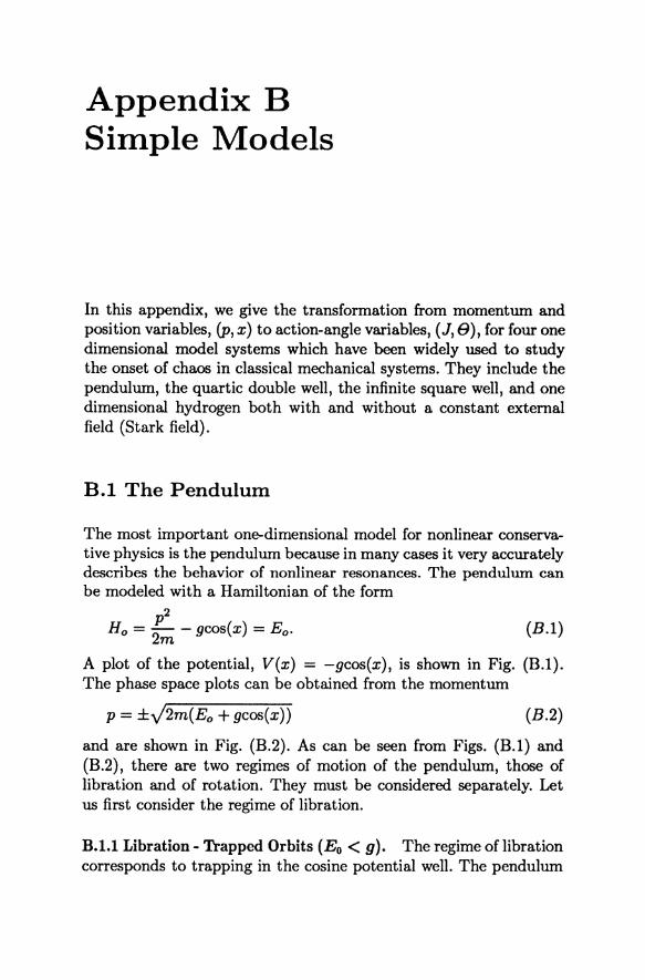
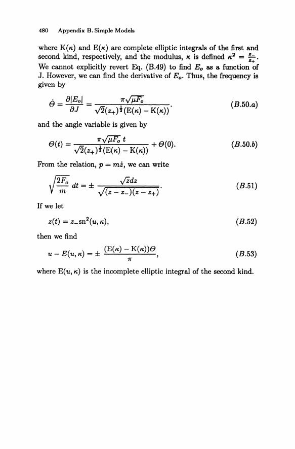
The most important one-dimensional model for nonlinear conservative physics is the pendulum because in many cases it very accurately describes the behavior of nonlinear resonances. The pendulum can be modeled with a Hamiltonian of the form
p2 Ho = 2m - gcos(x) = Eo. (B.1)
A plot of the potential, Vex) = -gcos(x), is shown in Fig. (B.1). The phase space plots can be obtained from the momentum
p = ±..j2m(Eo + gcos(x» (B.2)
and are shown in Fig. (B.2). As can be seen from Figs. (B.1) and (B.2), there are two regimes of motion of the pendulum, those of libration and of rotation. They must be considered separately. Let us first consider the regime of libration.
B.1.l Libration - Trapped Orbits (Eo < g). The regime of libration corresponds to trapping in the cosine potential well. The pendulum

468 Appendix B. Simple Models
v (X)
-2n -n -Xl o Xl n X
2n
Fig.B.I. The pendulum: x versus V(x)=-gcos(x)
bob never goes over the top. In this energy regime the turning points of the orbit (the point where p=O) are given by
x± = ±arccos( _ ~o ).
The action for this case is defined
J = 2~ f pdx = y'!m 1:+ dx JEo + gcos(x)
= 8y'mg [E(K) _ K,2 K(K)], 7r
(B.3)
(B.4)
where K(K) and E(K) are the complete elliptic integrals of the first and second kind and K is the modulus, defined, K2 = E2:g. We cannot explicitly write the energy, Eo, as a function of J, but we can obtain the derivative of the energy and therefore the angle variable, 8. We find
. oEo 7r..;9 8 = oJ = 2 .;m K(K) , (B.5.a)
and therefore
7r..;9 8(t) = 2 .;m K(K) t + 8(0), (B.5.b)
where 8(0) is the value of 8(t) at time t=O.

B.l. The Pendulum 469
p
x
Fig. B.2. The pendulum: phase space plot for m = 1.
The canonical transformation between variables (p,x) and actionangle variables, (J,B), is easy to find. If we remember that p=mX, then we can write
(B.6)
If we make the change of variables, sin(~) = K sin(z), we find after some algebra
(B.7)
. [ (2K(K)8)] x = 2 sm -1 K sn 7r ' K • (B.8)
where sn is the Jacobi elliptic sn function. If we plug Eq. (B.8) into Eq. (B.2) for p we find

470 Appendix B. Simple Models
(B.9)
where cn is the Jacobi elliptic cn function. Eqs. (B.B) and (B.9) give the canonical transformation between canonical variables (p,x) and (J,B) for Eo < O.
B.l.2 Rotation - Untrapped Orbits (Eo> g). Orbits undergoing rotation do not have a turning point but travel along the entire x axis with oscillations in momentwn (cf. Fig. (B.2». The action variable for such an orbit may be defined
lj'lf . 4.Jmg J = -2 dxv'2m(Eo + gcos(x» = --E(It).
7r -'If 1t7r (B.lO)
where the modulus, It, is now defined 1t2 = E~ig. The frequency is
e=8Eo = 7rV9
8J ItK(It)..;m
and angle variable is given by
7rV9 B(t) = ItK(It)..;mt + 8(0).
(B.ll.a)
(B.ll.b)
The canonical transformation from variables (p,x) to (J.8) can be obtained as before. Using p=mx, we can write ( after a change of variables)
.!:. fgdt= d(j) . (B.l2) It Y;;' Vl - 1t2sin2(~)
Integrating we find sin (~) = sn (:~, It) or
(B.l3)
where we have made use of Eq. (B.l1.b). In Eq. (B.l3), am is the Jacobi elliptic amplitude function. If we substitute this into Eq. (B.2) for the momentwn we find
p = ±.J2m ~ dn(K(;)8, It). (B.l4)
and dn is the Jacobi elliptic dn function.
vex)
-8
B.2 Double Well Potential
B.2. Double Well Potential 471
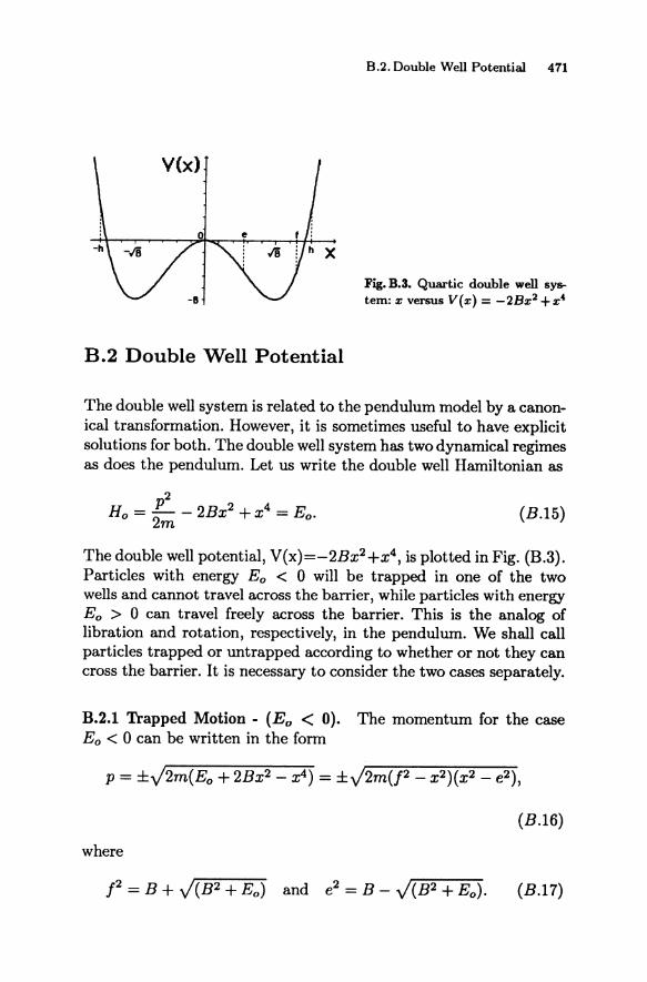
Fig. B.3. Quartic double well sy~ tern: z versus V(z) = -2Bz2 +z'
The double well system is related to the pendulum model by a canonical transformation. However, it is sometimes useful to have explicit solutions for both. The double well system has two dynamical regimes as does the pendulum. Let us write the double well Hamiltonian as
p2 Ho = 2m - 2Bx2 +x4 = Eo. (B.1S)
The double well potential, V{x)=-2Bx2+x4, is plotted in Fig. (B.3). Particles with energy Eo < 0 will be trapped in one of the two wells and cannot travel across the barrier, while particles with energy Eo > 0 can travel freely across the barrier. This is the analog of libration and rotation, respectively, in the pendulum. We shall call particles trapped or untrapped according to whether or not they can cross the barrier. It is necessary to consider the two cases separately.
B.2.1 Trapped Motion - (Eo < 0). The momentum for the case Eo < 0 can be written in the form
(B.16)
where
(B.17)

472 Appendix B. Simple Models
It is easy to see from Eq. (B.2) that x_ = e and x+ = J are the inner and outer turning points for particles trapped below the barrier. The action variable may be written
(B.18)
where the modulus It is defined 1t2 = tTl. From Eq. (B.18) we find that
e = aEo = V2/,rr aJ rm K(It)'
(B.19.a)
and the angle variable
V2J1r Bet) = rm K(It) t + $(0). (B.19.b)
The canonical transformation from variable (p,x) to (J,B) is o~ tained as follows. From the relation p = m:i; we can write
l ' dx = (21tdt = (2t x v(J2 - X 2)(x2 - e2 ) v;; 0 v;; .
We then obtain
( (2) ( K(It)$ ) X = J dn ±J V ;;t, It = J dn ± 1r ' It ,
(B.20)
(B.21)
where we have set $(0) = O. If we substitute Eq. (8.21) into Eq. (8.16), we find
p = ±J2mJ2lt2 sn(K(:)$, It) cn(K(:)$, It). (B.22)
B.2.2 Untrapped-(Eo > 0). The momentum for an untrapped particle can be written
p = ±V2m(Eo + 2Bx2 - x4) = ±..j2m(h2 - x 2)(X2 + 92),
(B.23)

B.2. Double Well Potential 473
-h o e .;Bfh X
Fig. B.4. Quartic Double Well System: Phase space plot for the quartic double well system.
where
The turning points of the motion are now given by x± = ±h. The action is given by
1 f v'2ffljh J = - pdx = -- dx..j(h2 - x2 )(X2 + 92) 211" 1I"_h
(B.25)
where K,'2 = (1 - K2) and the modulus, K, is defined K2 = h'J~9'J' From Eq. (B.17) we obtain
• 1I"h 8= .
../2m K K(K) (B.26.a)
and thus
474 Appendix B. Simple Models
v(x) 00
0 :",,' .' Fig. B.S. Square Well System: x versus V(x).
7rh B(t) = v'2ffl t + B(O).
2m K K(K) (B.26.b)
The canonical transformation is obtained in the usual manner. Since p = mx, we can write
l h dx (2 2KK(K)e x J(h2 - X 2)(x2 + g2) = V ;;;,t = e7r .
(B.27)
We therefore obtain
x = h cn(2K~)e, K), (B.28)
If we substitute Eq. (B.28) into Eq. (B.16), we find
p = ±v'2m ~ sn(2K~)e, K) dn(2K~)e, K). (B.29)
B.3 Infinite Square Well Potential
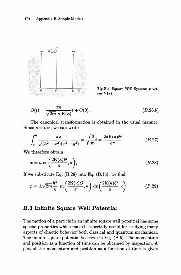
The motion of a particle in an infinite square well potential has some special properties which make it especially useful for studying many aspects of chaotic behavior both classical and quantum mechanical. The infinite square potential is shown in Fig. (B.5). The momentum and position as a function of time can be obtained by inspection. A plot of the momentum and position as a function of time is given

B.3. Infinite Square Well Potential 475
in Fig. (B.6). Analytic expressions are given in terms of the Fourier senes
pet) = J(2rnEo) sign [Sin (2;t) ]
,..,-_...,.... 4 00
= J(2rnEo) -; L n=l odd
1 . (271'nt) -sm --n T
and
or
4a x(t) = -a + -It I for
T ( - ::. < t < ::.) 22'
x(t) = _ 4a ~ ~cos(271'nt). 71'2 ~ n2 T
n=l odd
where T = ~ is the period of the motion.
(B.30)
(B.31.a)
(B.31.b)
In terms of the variables (P,X) the motion is discontinuous. A plot of p versus x is given in Fig. (B.7). The action variable is the area shown in Fig. (B.7). We find
J = ~fPdX = 2a~. 271' 71'
so that the Hamiltonian becomes
71'2J2 Ho=-S 2' rna
The angle variable can be obtained from
e _ oEo _ 71'2 J - oj - 4rna2'
or
71'2Jt 8(t) = -4 2 + 8(0).
rna
(B.32)
(B.33)
(B.34.a)
(B.34.b)

476 Appendix B. Simple Models
p
x
¥ t , , , "'"-
t
Fig. B.B. Square well system: (a) p versus t, (b) x versus t
p
-a a X
i:, .; !
a
b
~--~~--~' J2mEo Fig.B.7. Square well system phase space plot: p versus x
The canonical transformation from variables (p,x) and (J,B) can now be obtained from Eqs. (B.30) and (B.31). We find
p = J2mEo sign(sin(8)) (B.35)
and 2a
x = -a+ -181 for (-7T < 8 < 7T). 7T (B.36)

B.4. One-Dimensional Hydrogen 477
B.4 One-Dimensional Hydrogen
One-dimensional hydrogen is commonly considered both with and without an added constant field (Stark field). We shall consider both cases here.
B.4.1 Zero Stark Field. The Hamiltonian for one-dimensional hydrogen can be written
2 2 H - L _ Koe - E 0- 2p, z - 0,
(B.37)
where e is the charge of the electron, p, is the electron-proton reduced mass, and KO = 1/471'£0 (£0 is the permittivity constant). The range of
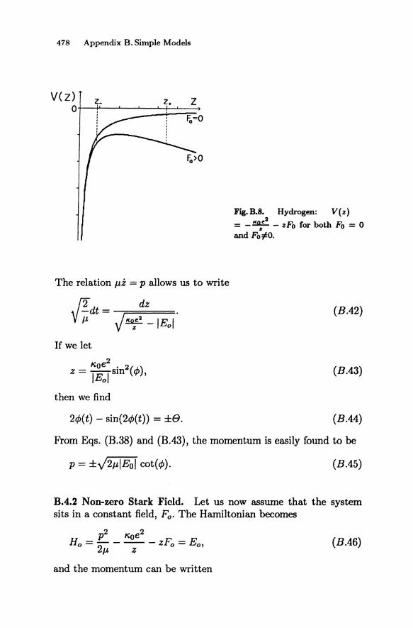
2 z is assumed to be O$z$oo. The potential, Vo(z) = - K.~e is plotted in Fig. (B.8). From Eq. (B.37) the momentum can be written
;0::. / Koe2 p = ±y2P,V -IEol + -z-· (B.38)
When the energy Eo < 0, the particle is in a bound state. It reverses its momentum abruptly at z=O and has an outer turning point at
2
ZT = i~: I . The action is defined
1 f . /2 IE I lK.oe2/lEol dz J = _ pdz = V P, 0
271' 71' JZ
Koe2yTi = yf2l Eol'
Therefore in terms of action variable, J, the Hamiltonian is
-p,K02e4
Ho = 2J2 = Eo.
The angle variable, B, is obtained from
That is
(B.39)
(BAO)
(BAl.a)
(B.4l.b)
478 Appendix B. Sjmple Models
vez) °ti-'---~~~=2
z. z
The relation p,z = p allows us to write
fid dz V j;,' t = J It°ze
2 -IEol'
If we let
then we find
2</>(t) - sin(2</>(t» = ±e.
Fig.B.B. Hydrogen: V(z) "0,,2 = - I: - zFo for both Fo = 0
and Fo¢O.
(B.42)
(B.43)
(B.44)
From Eqs. (B.38) and (B.43), the momentum is easily found to be
p = ±/2p,IEol cot(</». (B.45)
B.4.2 Non-zero Stark Field. Let us now assume that the system sits in a constant field, Fo. The Hamiltonian becomes
p2 Koe2 Ho = 2p, - -z- - zFo = Eo, (B.46)
and the momentum can be written
B.4. One-Dimensional Hydrogen 479
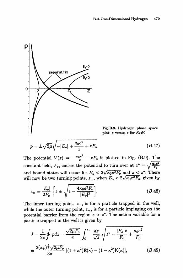
Fig. B.9. Hydrogen phase space plot: p versus z for Fo:#O
(B.47)
The potential V{z) = - K.oze2
- zFo is plotted in Fig. (B.9). The
constant field, Fo , causes the potential to turn over at z* = J K.}:2
and bound states will occur for Eo < 2"; ltoe2 Fo and z < z*. There will now be two turning points, z±, when Eo < 2Jltoe2Fo, given by
z± = IEol [1 ± 2Fo
(B.4S)
The inner turning point, z_, is for a particle trapped in the well, while the outer turning point, z+, is for a particle impinging on the potential barrier from the region z > z*. The action variable for a particle trapped in the well is given by
J=..!..f dz= ~ r- dz 27r P 7r Jo Vi
(B.49)
480 Appendix B. Simple Models
where K(I\:) and E(I\:) are complete elliptic integrals of the first and second kind, respectively, and the modulus, I\: is defined 1\:2 = :~. We cannot explicitly revert Eq. (BAg) to find Eo as 8 function of J. However, we can find the derivative of Eo. Thus, the frequency is given by
(B.50.a)
and the angle variable is given by
(B.50.b)
From the relation, p = mi, we can write
J2Fo dt = ± ftdz . m J(z - z_)(z - z+)
(B.51)
If we let
z(t) = z_sn2(u, 1\:), (B.52)
then we find
(B.53)
where E(u, 1\:) is the incomplete elliptic integral of the second kind.
Appendix C Renormalization Integral
The technique for evaluating the integral
1 jM1f Vn(J,lI) = -2 d8 cos[lIx(J,8) - (11 + n)8],
7r -M1f where 11 = ~ (N and M integer) and
(C.1)
is given in [Smith and Pereira 1978] and [Escande and Doveil (1981)]. K(I\:) is the complete elliptic integral of the first kind and I\: is the modulus. We will sketch the method here. If 11 is an integer (M = 1) then an exact expression for Vn(J,lI) can be found. If 11 is not an integer, then a rapidly converging expansion of Vn(J, 11) in terms of
K' the nome, q = e-.... Y , (where K'(K) = K(K') with K,2 = 1- K2) can be obtained. Let us first consider the case when 11 is an integer.
C.l V = N=integer
Since x is an odd function of 8 we can write Eq. (C.1) in the form
Vn(J, N) = 2.j1f d8 ei [2N am(¥)-(N+n)8) 27r -1f
(C.2)
where
482 Appendix C. Renormalization Integral
. (Ki) (KO). (KO ) f(O) = e,am,. = cn 7' K, + tsn 7' K, , (C.3)
and cn and sn are Jacobi elliptic functions. Let us now make the change of variables u = ~9. Then Eq. (C.2) takes the form
Vn(J, N) = ...!..j7r dO ei[2N ame~n-(N+n)91 21r -7r
= _l_jK du [cn(u) + i sn(u)J2N e-i(N+n)¥. 2K -K
(CA)
We can evaluate Eq. (CA) using the contour shown in Fig. (C.1). The pole at u = iK' gives no contribution while the pole at u = i3K' does give a nonzero result. The contributions from the two vertical sides of the contour cancel. We find that
1 (.)2N Vn(J, N) = -(21ri) (1 _ qi(N+n») (2N _ 1)! ~
. d2N-1 [ -o,.K. (dn(s) + 1)2N] x lim e~ . 8-+0 ds2N -1 sn( s)
(C.5)
To obtain Eq. (C.5) we have made the change of variables u = s + 3iK' and have used the fact that [Byrd and Friedman 1971]
sn(s + 3iK') = sn(s + iK') = \) K,sn s
and
. . idn(s) cn(s + 3tK') = -sn(s + tK') = ( r K,sn s
We can now expand sn(s) and dn(s)in powers of s. For lsi < K', we can write
and
We then obtain

C.2. II = Z ~integer 483
1m u -K+4iK' K+4iK'
o 3iK'
c
o jK'
-K o K Re u Fig. C.l. Integration contour
d2N-1 [ -."K. ( 1 - lC~f' + 0(s4) )2N] X lim e ~ --=.....:;.,..,....,,-..;.,.-~
8-+0 ds2N-1 1 _ (1+;;)82 + 0(s4) , (C.6)
Let us evaluate Eq. (C.6) for the special case, N=1. We find
(C. 7)
Explicit expressions for Vn (J, N) for N > 1 can be obtained from Eq. (C.5) or (C.6).
C,2 V = ~ ;6 integer
Let us first write Vn(J, 1/) in the form
Vn (J,1/) = ...!...jM1r dO ei[211 am(~'I)-(II+n)81 27r -M1r
(C.8)
where f(O) is defined in Eq. (C.3). We will need expansions of en and sn in terms of the nome, q [Byrd and Friedman 1971). They are given by
27r 00 qm+t Ku cn(u, K) = -K( ) :L 2 +I cos[(2m + 1)-2 1
K K m=O 1 + q m 7r (C.g.a)
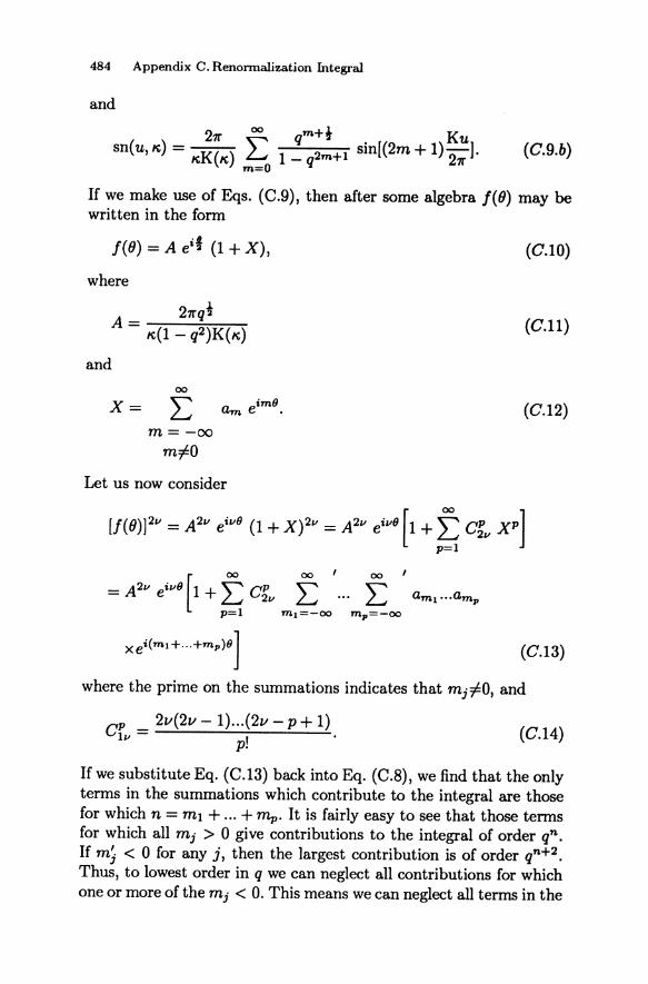
484 Appendix C. Renonnalization Integral
and
21r 00 qm+i Ku sn(u, K) = KK(K) f. 1 _ q2m+1 sin[(2m + 1) 21r]' (C.9.b)
If we make use of Eqs. (C.g), then after some algebra f(O) may be written in the form
f(O) = A eif (1 + X), (c. 10)
where
(C.11)
and 00
X= 2: (C.12)
m=-oo m;fO
Let us now consider
(C.13)
where the prime on the summations indicates that mj;fO, and
Cp _ 21/(21/ - 1) ... (21/ - P + 1) Iv - I . p.
(C.14)
If we substitute Eq. (C.13) back into Eq. (C.S), we find that the only terms in the summations which contribute to the integral are those for which n = ml + ... + mp. It is fairly easy to see that those terms for which all mj > 0 give contributions to the integral of order qn. If mj < 0 for any j, then the largest contribution is of order qn+2. Thus, to lowest order in q we can neglect all contributions for which one or more of the mj < O. This means we can neglect all terms in the

C.3. References 485
summation for which p > n. Let us now consider all terms for p < n. There are in fact C~=~ contributions such that ml + ... + mp = n with mj > O. Thus we finally obtain, to lowest order in q,
where n
r'I' _ ""' CP rrP-I LJ n - ~ 21' un-I'
p=l
(C.15)
(C.16)
Because expansions in the nome generally converge rapidly (for K, = 0.1, q = 0.0006; for K, = 0.5, q = 0.0180; for K, = 0.9, q = 0.1024) Eq. (C.15) gives a very good approximation to the amplitude Vn(J, v).
C.3 References
Byrd, P.F. and Friedman, D. (1971): Handbook of elliptic Integrals for Engineers and Scientist (Springer-Verlag, Berlin).
Escande, D.F. and Doveil, F. (1981): J. Stat. Phys. 26 257. Smith, G.R. and Pereira, N.R. (1978): Phys. Fluids 21 2253.

Appendix D Moyal Bracket
For quantum mechanical systems the momentum operator, p, and position operator, q, do not commute,
[q,p] = qp - pq = in, (D.I)
and therefore it is not possible to specify simultaneously the momentum and position of a particle in phase space. However, Wigner [Wigner 1932] showed that it is possible to develop a theory of quantum systems in phase space which is formally analogous to classical theory. Moyal [MoyaI1949] further developed this theory and showed that the equations of motion and commutation relations between arbitrary operators, A(p, ij), which are functions of operators, p and ij, could be expressed in terms of phase functions, A(p, q), which reduce to the correct classical functions when n--+O.
D.1 The Wigner Function
Following Moyal, let us consider a system in state, It/J), and introduce the characteristic operator
(D.2)
where T and </> have units of position and momentum, respectively. For simplicity of notation, we consider a one degree of freedom system in this Appendix, but our results are easily generalizable to many degrees of freedom. For a system in state It/J), the characteristic operator has expectation value
(D.3)
D.l. The Wigner Function 487
where M(T,</J) is the characteristic function for a system in the state It/J}. In Eq. (D.3), we have used the relation
(DA)
for operators, A and 13, which commute with their commutator, [A,13J. We denote the eigenstates of p and q by Ip) and Iq), respectively. That is, pip) = pip) and qlq) = qlq). In the position representation, p = -in/q while in the momentum representation, q = in gp' If we use the completeness relation, 1 = I dqlq)(ql, then we may write the characteristic function in the form
(D.5)
The Fourier transform of M (T, </J) is just the Wigner function
f(p,q) = - dTd</J M(T,</J) e-t(Tp+.pq). 1 100 100 .
27rn -00 -00
(D.6)
The Wigner function, f(p, q), is formally analogous to the classical probability density on phase space [Reichl 1980], and reduces to it in the limit n~O. However, the Wigner function is not always positive and therefore does not have the meaning of a probability density except in the classical limit.
An arbitrary operator, A(p, q), can also be related to a phase function, A(P, q). We write
A(p, q) = _1_100 100 dTd</J aCT, </J) et(TP+.pq). 27rn -00 -00
(D.7)
(This type of expression was first obtained by Weyl [Weyl1931J. See also [Littlejohn 1986J.) Then, the phase function, A(p, q), is defined
1 100 100 . A(p, q) = 27rn -00 -00 dTd</J aCT, </J) et(Tp+.pq). (D.8)
so that
A ( 1 )2100 100
A(p, q) = 27rn -00'" -00 dTd</Jdpdq A(p, q)
(D.9)
If we take the expectation value of A(p, q) with respect to the state It/J), we find from Eqs. (D.3), (D.6), and (D.9)

488 Appendix D. Moyal Bracket
~ 1 roo roo (1/JIA(p,q)I1/J) = 27rhJ_ooJ_oo dpdq A(p,q) f(p,q)· (D.10)
Thus the operators, A(p, q), have been expressed in terms of the phase functions, A(p,q), and the state of the system is represented by the Wigner function, f(p,q). (Jensen and Niu [Jensen and Niu 1990] have used momentum and position phase functions, closely related to A(p, q), to study the delta-kicked rotor.)
D.2 Ordering of Operators
If we are given a phase function, A(p,q), there is a method for obtaining the corresponding operator, A(p, q), with the correct ordering of momentum and position operators, p and q. Let us first note that using Eqs. (D.3) and (D.4), we can write the characteristic function as
M(r, </J) = (1/JlettPQet7'PeH'7'tPl1/J)
= 1:1: dqdp(1/Jlq){qlp){pl1/J)e,;I;£-et<7'P+tPq) ,
(D.ll) where we have inserted completeness relations for the states, Ip > and Iq >. Note that < qlp >= (27rh)-i et pQ. Integrating Eq. (D.ll) by parts, we find
M(r, </J) = 1:1: dpdqe*(7'P+tPQ)e~;I;/q x (1/Jlq) (qlp){pl1/J).
Thus the Wigner function takes the form
!(p, q) = 27rhett l;/q (1/Jlq){qlp) (P11/J)·
Let us now use Eq. (D.13) to rewrite Eq. (D.lO) in the form
(1/JIACP, q)I1/J) = 1:1: dpdq (1/Jlq){qlp)(PI1/J)
x {e~'I;/q A(p, q)},
(D.12)
(D.13)
(D.14)

D.2. Ordering of Operators 489
where we have integrated by parts. We next rewrite A(P, q) as follows. Let A(p, q)-+Ao(q,p), where in Ao(q,p) all p dependent tenns explicitly lie to the right of q dependent tenns. Ao(q,p) is said to have "standard" ordering. This rearrangement makes no difference in Eq. (D.14), but allows us to write Eq. (D.14) in the following fonn
(1/JIA(P, q)I1/J) = i:i: dpdq(1/Jlq)(qlp) (P11/J)
x {et,1,;1q Ao(q,p) }
= i:i: dpdq(1/Jlq)(qlp) { ei;l,;£- Ao(q,p) } (P11/J)
= (1/JI{ et '4ItAo(p,q) }11/J). (D.15)
The bracket, U, indicates that the derivatives act only on functions inside the bracket. Thus, we find
(D.16)
Eq. (D.16) gives us the operator, A(p, q) with the correct ordering of p and q.
To see how this works, let us consider the following example. Suppose we are given the phase function, A(P, q) = p2q2 and we wish to find the correct operator, A(p, q), corresponding to this phase function. First we write Ao(q,p) = q2p2. Then
(D.17)
If we now make use of the commutation relation, Eq. (D.l), we find
AA(A A) A2A2 2·t;AA It;2 1{~2A2+2AA2A+ A2A2) (D.18) p, q = q p - tnqp - 2'~ = '4V' q pq p q p
as we would expect.

490 Appendix D. Moyal Bracket
D.3 Mayal Bracket
We now wish to express the commutation relation
(D.19)
in terms of the phase functiops, C(P,g), A(p,q), 8.!ld B(P, q) which are associated with operators, C(p, q), A(P, q), and B(P, q), respectively, via Eq. (D.9). From Eq. (D.7), Eq. (D.19) can be written
= (2~h)2i:i:dTldT2d¢ldtP2 a(TlJ¢l) b(T2,4>2)
x [et('T1P+4>lQ), et('T2P+4>:aQ)]. (D.20)
However, from Eqs. (D.I) and (D.4) the commutator in Eq. (D.20) is given by
= 2i e*(('Tl+1'2)P+(4>1+4>:a)Q)sin[2~ (Tt¢2 - T2¢t)]. (D.21)
If we substitute Eq. (D.21) into Eq. (D.20) and take the expectation value of Eq. (D.20) with respect to the state 11/1 >, we obtain
XSin[21h (Tl¢2 - T2(1)]M(TI + T2, ¢1 + 4>2). (D.22)
We next use Eqs. (D.6) and (D.B) to find
1 100 100 ih27rh -00 -00 dpodqo C(Po, qo) f(Po, qo)
= 2i(2~h) 3 i: ... i: dTldT2d¢ld¢2dpdq f(P,q)

D.4. References 491
xsin[211i (TI<P2 - T2<PI)]
xa(T}, <PI) et("T1P+<Plq) b(T2' 4>2) e t ("T:lP+4>2q)
= - dpdq j(p,q) sm - -----( 2i ) 100 100 • [Ii (0 0 0 0) ]
21r1i -00 -00 2 OPB oqA OPA OqB
xA(p, q) B(p, q),
(D.23)
where aa and.,J..- operate on the function A(p, q) and -,ft- and -,ft-PA oqA OPB OPB
operate on the function B(p, q). From Eq. (D.23), we find that the phase function equivalent to the commutator Eq. (D.19) is the phase function relation
iliC(p, q) = (2i)sin [~( 8~A 8:B - 8:A 8~B) ] A(p, q)B(p, q).
(D.24)
Eq. (D.24) was first derived by Moyal and called the Moyal bracket. In the limit, Ii-+O, Eq. (D.24) reduces to
C(p q) = 8A8B _ 8A8B , 8q 8p 8p 8q'
which is just the Poisson bracket.
D.4 References
Jensen, J.H. and Niu, Q. (1990): Phys. Rev. A42 2513. Littlejohn, R.G. (1986): Phys. Rept. 13 193. Moyal, J.E. (1949): Proc. Cambridge Phil. Soc. 45 99.
(D.25)
Reichl, L.E. (1980): A Modem Course in Statistical Physics (University of Texas Press, Austin; Edward Arnold Pub., London; Peking University Press, Beijing; Marzuden Pub., Tokyo).
Weyl, H. (1931): The Theory of Groups and Quantum Mechanics(Dover Pub., New York).
Wign~r, E. (1932): Phys. Rev. 40 749.
Appendix E SU(3)
Roughly speaking, Lie groups are groups consisting of group elements, R;,(O) = ei8g• which are labeled by one or more continuous variables, Oi, each of which has a well defined range [eahn 1984], [Jacobson 1962], [Humphreys 1972]. The quantities, gi, are the infinitesimal generators of the Lie group, and can be determined from the behavior of the group elements near the identity (for 0«1). The structure of a given Lie group is determined by its group multiplication rules. Near the identity transformation the group multiplication rules lead to commutation relations on the generators, gi, namely
[gi, gil = L:€~ gk) (E.1) k
where €~ is a structure constant. The commutation relations are equivalent to the group multiplication rules and all essential information about local properties of the Lie group are contained in the structure constants, €~ • To fully specify possible representations of the Lie group, one may in addition need to know some global properties. For example, for the rotation group one might require Ri(O) = Ri(0+27r), which is global property of the system considered.
E.l Special Unitary Groups
The Lie group, SU(n), is the special unitary group whose representation of smallest dimension consists of n x n dimensional unitary matrices with determinant one. The generators of SU(n) can be re~ resented by traceless Hermitian matrices.
The group SU(2) has three generators, jx, jy, and jz since there are three linearly independent 2 x 2 traceless Hermitian matrices. It

E.1. Special Unitary Groups 493
is convenient to use non-Hermitian combinations of these generators, j+ = jx + ijy, j- = jx - ijy, and jz as generators of SU(2). These generators satisfy the Lie algebra
and have the 2 x 2 dimensional representation
- (1 0) Jz = 0 -1 '
- (0 1) J+ = 0 0 '
The Lie algebra of SU(2) is identical to that of the group 0(3) of rotations in three dimensions although the two groups are not identical.
The group SU(3) consists of eight generators since there are eight linearly independent 3 x 3 traceless Hermitian matrices. It is again convenient to use non-hermitian combinations of these generators. We shall denote the generators as hI, h2 , et, ei with i = 1,2,3. These generators satisfy the Lie algebra
[et,ejJ = oi,jhj (i,j = 1,2)
(E.2)
where Oi,j is the Kronecker delta function and Kij is the (ij)th element of the Cart an matrix, k, for the Lie group, SU(3). The Cartan matrix is given by
- (2 K= -1
-1) 2 . (E.3)
The generators, hI and h2' form a two dimensional subalgebra, called the Cartan subalgebra, which is abelian ([hI, h2J = 0 so group elements commute).
The eight generators of SU(3) may be represented by the following 3 x 3 matrices.
(1 0 0) (0 0 0) HI = 0 -1 0 , H2 = 0 1 0 ,
o 0 0 0 0 -1
(0 1 0) (0 0 0) Et = 0 0 0 , Et = 0 0 1 , o 0 0 0 0 0
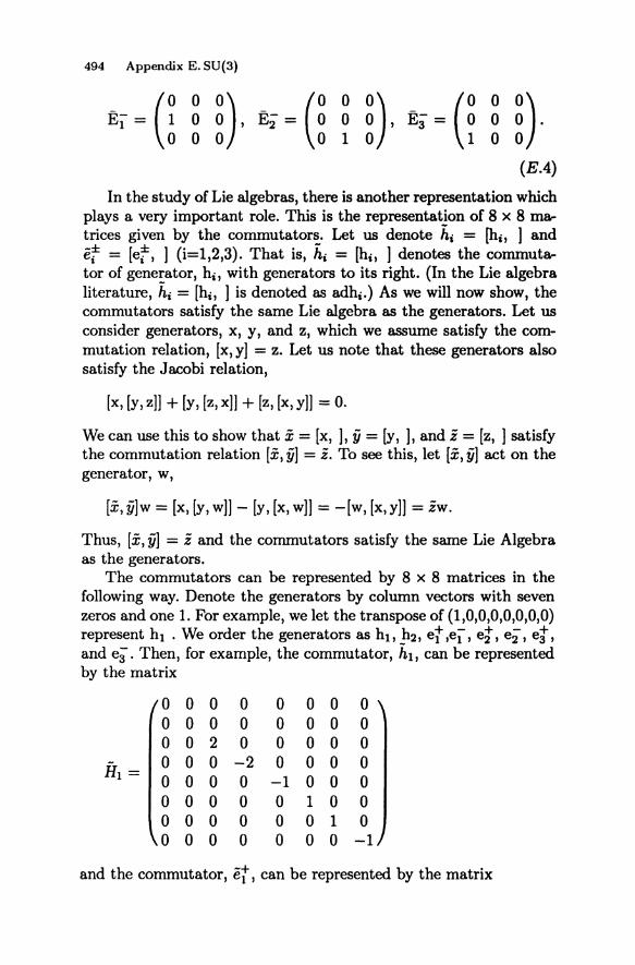
494 Appendix E. SU(3)
COO) ~=G 0
n· 0 0
n· EI = 1 0 0 , 0 E;= 0 000 1 0
(E.4)
In the study of Lie algebras, there is another representation which plays a very important role. This is the representation of 8 x 8 matrices given by the commutators. Let us denote hi = [hi, land et = [et, 1 (i=1,2,3). That is, hi = [hi, 1 denotes the commutator of generator, hi, with generators to its right. (In the Lie algebra literature, hi = [hi, 1 is denoted as adhd As we will now show, the commutators satisfy the same Lie algebra as the generators. Let us consider generators, x, y, and z, which we assume satisfy the commutation relation, [x, y] = z. Let us note that these generators also satisfy the Jacobi relation,
[x, [y, zlJ + [y, [z, xlJ + [z, [x, ylJ = o.
We can use this to show that x = [x, ], ii = [y, ], and z = [z, 1 satisfy the commutation relation [x, iil = z. To see this, let [x, iil act on the generator, w,
[x, iilw = [x, [y, wlJ - [y, [x, wlJ = -[w, [x, ylJ = zw.
Thus, [x, iil = z and the commutators satisfy the same Lie Algebra as the generators.
The commutators can be represented by 8 x 8 matrices in the following way. Denote the generators by column vectors with seven zeros and one 1. For example, we let the transpose of (1,0,0,0,0,0,0,0) represent hI . We order the generators as h}, h2' et ,eI , et, e2", et, and ei. Then, for example, the commutator, hI, can be represented by the matrix
0 0 0 0 0 0 0 0 0 0 0 0 0 0 0 0 0 0 2 0 0 0 0 0
HI = 0 0 0 -2 0 0 0 0 0 0 0 0 -1 0 0 0 0 0 0 0 0 1 0 0 0 0 0 0 0 0 1 0 0 0 0 0 0 0 0 -1
and the commutator, et, can be represented by the matrix
E.1. Special Unitary Groups 495
0 0 0 1 0 0 0 0 0 0 0 0 0 0 0 0
-2 1 0 0 0 0 0 0
E+ - 0 0 0 0 0 0 0 0 1 - 0 0 0 0 0 0 0 0
0 0 0 0 0 0 0 -1 0 0 0 0 1 0 0 0 0 0 0 0 0 0 0 0
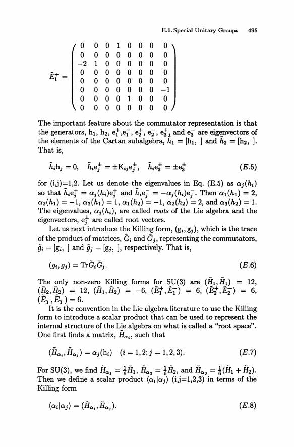
The important feature about the commutator representation is that the generators, hI, h2 , et ,eI , et, e2', et, and e; are eigenvectors of the elements of the Cartan subalgebra, hI = (hI, ] and h2 = [h2 , ].
That is,
(E.5)
for (iJ)=1,2. Let us denote the eigenvalues in Eq. (E.5) as Ctj(hi) so that hiej = Ctj(hi)ej and hiej = -Ctj(hi)ej. Then Ctl(hl) = 2, Ct2(hl) = -1, Ct3(hl) = 1, Ctl(h2) = -1, Ct2(h2) = 2, and Ct3(h2) = 1. The eigenvalues, Ctj(hi ), are called roots of the Lie algebra and the eigenvectors, ej are called root vectors.
Let us next introduce the Killing form, (gi, gj), which is the trace of the product of matrices, Gi and G j, representing the commutators, 9i = [gi' ] and 9j = [gj, ], respectively. That is,
(E.6)
The only non-zero Killing forms for SU(3) are (Ht, HI) = 12, (H2' H2) = 12, (Ht, H2) = -6, (Et, En = 6, (Et, E2") = 6, -+ --(E3 ,E3 ) = 6.
It is the convention in the Lie algebra literature to use the Killing form to introduce a scalar product that can be used to represent the internal structure of the Lie algebra on what is called a "root space" . One first finds a matrix, Ho " such that
(E.7)
- 1- - 1- - 1- -For SU(3), we find HOI = '6HI, H02 = '6H2, and H03 = '6(H1 + H2). Then we define a scalar product (CtiICtj) (iJ=I,2,3) in terms of the Killing form
(E.8)

496 Appendix E. SU(3)
--------~-------+a1
Fig. E.l. The root vectors of SU(3)
For SU(3) we obtain (allal) = (a2Ia 2) = l, (alla2) = (a2Ial) = -i, and (alla3) = (a3Ia l) = i· The vectors, laj), (i=1,2,3) are vectors on the "root space" and can be thought to geometrically represent the roots and therefore the internal structure of the Lie algebra. For example, for SU(3), the scalar products indicate that
the vectors lai) (i=1,2,3) have length Ii. The angle between lal)
and l(2) is 120° while that between lal) and l(3) is 60°. Thus we can represent SU(3) by the picture shown in Fig. (E.1).
Notice that H03 = HOI + Ha~, a3(hi ) = al(hi ) + a2(hi ) and l(3) = lal) + l(2). Thus all properties of the root space can be determined in terms of just HOI and Ho~ (lal) and l(2). These are called the simple roots.
E.2 References
Cahn, R.N. (1984): Semi-Simple Lie Algebras and Their Representations (Benjamin-Cummings Pub. Co., Menlo Park, Calif.).
Jacobson, N. (1962): Lie Algebras (J. Wiley and Sons, New York). Humphreys, J.E. (1972): Introduction to Lie Algebras and Represen
tation Theory (Springer-Verlag, Berlin).
Appendix F Space-Time Symmetries
Let us consider an N particle system described by a Hamiltonian, H(t) = H( {Pi}, {iid, {sd, t), where Pi and iii are the momentum and position operators for the ith particle and Si is the spin of the ith particle. The equation of motion for a quantum operator, O(t), in the Heisenberg picture is
A A
dO 80 iA A dt = at + r;:[H(t), OCt)]. (F.1)
If the Hamiltonian contains no explicit dependence on time then dd~ = a and H is a constant of the motion. There are a number of space-time symmetries which lead to additional constants of the motion [Messiah 1962]. We discuss some of them below. However, it is useful to first summarize some properties of linear and antilinear operators.
F.1 Linear and Antilinear Operators
All of the operators we deal with in this book are linear except for the time reversal operator which is antilinear. In this section, we distinguish between linear and antilinear operators.
F.1.1 Linear Operators. Let us consider a linear operator, O. When acting on a state 1!Ii') = cll'I/Jl) + c21'I/J2), where Cl and C2 are complex constants, we find
Scalar products behave as
498 Appendix F. Space-Time Symmetries
«(xIO)I'I/J) = (xl(OI'I/J)· (F.3)
Scalar products involving the hermitian adjoint of a linear operator behave as
(FA)
Let us now contrast the behavior of linear operators with those of antilinear operators
F .1.2 Antilinear Operators. Let us consider the antilinear operator, A.. When acting on the superposition l\li) = cll'I/Jl) + C21'1/J2), it gives
A.1\li) = A.(cll'I/Jl) + c21'I/J2) = cl*(AI'l/Jl» + C2*(AI'l/J2)' (F.5)
Scalar products behave as
(F.6)
and scalar products involving the hermitian adjoint behave as
(F.7)
This distinction between linear and antilinear operators is important when we talk about the effects of time reversal, which is an antilinear operator.
F.2 Infinitesimal Transformations
Let us consider infinitesimal transformations on the system implemented by the unitary operator, T(6a), which has the property that T(6a)-+1 as 6a -+ O. We can write
T(6a) ~ 1 + iB6a, (F.8)
where e is a hermitian operator (since T(6a) is unitary). e is the called the generator of the infinitesimal transformation. Let us assume that an operator, 0, is changed to 0' = 0 + 60 by the transformation. That is,
T(6a)0i't (6a) = 0' = 0 + 60 ~ 0 + ire, Ol6a + ... (F.9)
Then to lowest order in the deviations, 60 = +i[e, Ol6a and
F.2.1. Time Translation 499
06 A A
00! = +i[8, OJ. (F.lO)
For arbitrary oo! we find
T(oO!) = e+i8cSQ •
Let us now consider some specific examples.
F.2.1 Time Translation
(F.ll)
If we translate the operator, 6, forward in time then 00! = ot and
00 A A
Tt = +i[e,Oj. (F.l2)
Thus, e = * if and therefore the Hamiltonian is the generator of infinitesimal translations in time. The time translation operator is given by
T(ot) = etff.cSt (F.l3)
for the case when if has no explicit time dependence.
F .2.2 Space Translation. Let us now translate the system in space by a fixed displacement, oa. Then T(oa)CtiTt(oa) = Cti + oa and
OCti '[Q A J 6; = t o,qi . (F.l4)
If e is to give a similar result for each Cti then e = Pin, where P is the total momentum, P = Ed)i' Thus, the total momentum is the generator of translations in space. The transformation operator is given by
(F.l5)
For the case of a Hamiltonian, H({pd, {Ctij}, {sdt), which depends only on the relative displacements of particles, Ctij = Cti - iii, we find
(F.l6)
so that [H, Pj = 0 and the total momentum, P is constant of the motion.
500 Appendix F. Space-Thne Symmetries
F .2.3 Rotation. Let us now consider rotations of the system through an angle, 6</>, about an axis given by unit vector, n. Then
(F.17)
and
(F.18)
For simplicity, let us consider a Hamiltonian of the form II = 2!nEiP; + V({qi}). Then ~ = ik[lI,pil and ~ = -ik[lI,qil so we can write
A A A t A ~ (dPi dqi ) T(6</>n)HT (6</>n) = H + ~ - di·6qi + di·6Pi + ... (F.19) I
If we let 6qi = -6</>nxqi and 6Pi = -6</>nxPi in Eq. (F.19), we find
T(6</>ft)iI'i't(6</>ft) = II + 6</>ft· ~~ = II + *6</>n.[Ji,Ll, (F.20)
where L = EAiXPi is the total angular momentum. Thus from Eq. (F.9) we obtain e = Land L is the infinitesimal generator of rotations. If 6H = 0 then ~~ = 0 and L is a constant of the motion. The rotation operator is given by
(F.21)
For the case when particles have spins, {Si}, the infinitesimal generator of rotations is given by the total angular momentum
(F.22)
and the rotation transformation generalizes to
(F.23)

F.3. Discrete Transfonnations 501
F.3 Discrete Transformations
Discrete transformations cannot occur by an infinitesimal amount. They either occur or they don't.
F.3.1 Parity. The group of reflections through a point has two elements, the identity element, I, and the reflection, Po (the parity operator). Under reflection, polar vectors, p and 'I, change sign while axial vectors, j remain unchanged. Thus,
(F.24)
From this we see that the parity operator commutes with the rotation operator.
F.3.2 Time Reversal. The time reversal operator, K, is an antiunitary operator. When operators are written in the coordinate representation, it can be written as the product of the complex conjugat!on operAator, Ko (KoiK~ = -i) and a unitary operator, T so that K = K oT. The effect of time reversal is
KpKt = -p, KqKt = 'I, and KjKt = -1 (F.25)
Thus, time reversal commutes with the rotation operator
(F.26)
(since both i and J change sign). If no spins are present, then K = Ko (in the coordinate representation). However, if we look at the effect of time reversal on Pauli spin matrices, we find
Thus, in order to have KSiKt = -Si we must include a unitary operator, T which has the following effect on coordinate and spin operators
TpTt = p, TqTt = it, (F.28)
and
(F.29)
502 Appendix F. Space-Time Symmetries
This can be accomplished by choosing t = e-f1l"811 • If the total spin is S = LiSi then t = e-f1l"SIl and the time reversal operator is given by
(F.30)
Let us now consider the square of k,
k2 = e-f1l"slI koe-f1l"SIl ko = e-f211"SII. (F.31)
We can evaluate k2 with respect to the basis IS, Sy}. Then for integer total spin, k2 = +1, while for half-integer total spin, k2 = -1. This has important consequences regarding the form of the Hamiltonian matrix for time reversal invariant systems.
F.4 References
Messiah, A. (1964): Quantum Mechanics (North-Holland Pub. Co., Amsterdam)
Appendix G GOE Spectral Statistics
In this appendix we will demonstrate the various steps necessary to obtain a usable expression for the generating function, RN(l), for the case of a Gaussian orthogonal ensemble. We will first consider the function, ~(l), and then quote the results for the more general case, RN(l). Once we have obtained, RN(l), we can obtain explicit expressions, in terms of orthonormal oscillator wave functions, for the cluster functions, Tl(X) and T 2(x,y).
G.l The Generating Function R4(1)
From Eq. (6.4.9) the generating function, R4 (1), can be written in the form
Because the integrand is unchanged under permutation of indices we can rewrite the energy integrations in an energy ordered form if we also multiply by 4!, the number of permutations. We may also write the product of energy differences in terms of a Vandermonde determinant. We find
/ 00 /00 [ 4 1 4 ] R4(1) =4! C4 -00'" -00 dx1 ... dx4 g(l+ai )] exp[-2~X:
x(}(oo - X4)(}(X4 - X3)(}(X3 - X2)(}(X2 - Xl)(}(Xl + 00)
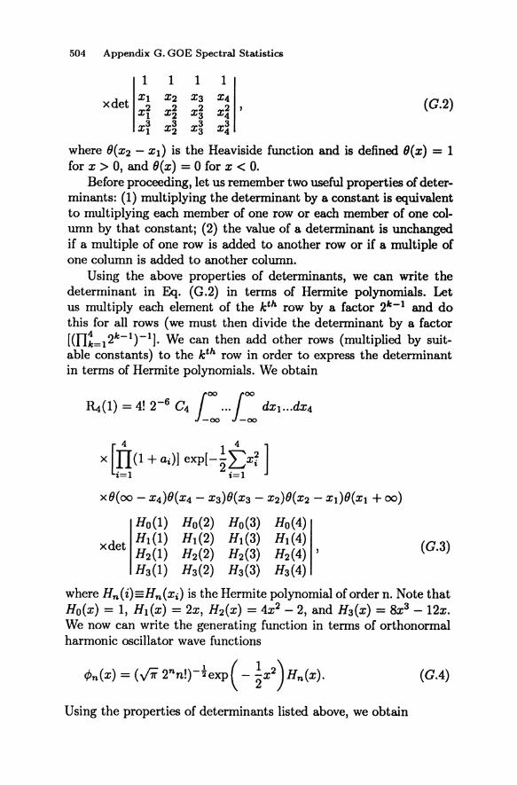
504 Appendix G. GOE Spectral Statistics
1 1 1 1
xdet Xl X2 X3 X4 (G.2) xi x~ x2 x~ ,
3
X~ X~ X3 3 X~
where 8(X2 - Xl) is the Heaviside function and is defined 8(x) = 1 for X > 0, and 8(x) = 0 for X < o.
Before proceeding, let us remember two useful properties of determinants: (1) multiplying the determinant by a constant is equivalent to multiplying each member of one row or each member of one column by that constant; (2) the value of a determinant is unchanged if a multiple of one row is added to another row or if a multiple of one column is added to another column.
Using the above properties of determinants, we can write the determinant in Eq. (G.2) in terms of Hermite polynomials. Let us multiply each element of the kth. row by a factor 21c - 1 and do this for all rows (we must then divide the determinant by a factor [(n!=121c- 1 )-1]. We can then add other rows (multiplied by suitable constants) to the kth. row in order to express the determinant in terms of Hermite polynomials. We obtain
[ 4 1 4 ]
x !! (1 + ai)] exp[-2~X;
x8(00 - x4)8(X4 - x3)8(X3 - x2)8(X2 - Xt>8(XI + 00)
xdet
Ho(1) HI(I) H2 (1) H3(1)
Ho(2) H I (2) H2(2) H3(2)
Ho(3) HI (3) H2(3) H3(3)
Ho(4) HI (4) H2 (4) , H3(4)
(G.3)
where Hn(i)=Hn(Xi) is the Hermite polynomial of order n. Note that Ho(x) = 1, HI(X) = 2x, H2(X) = 4x2 - 2, and H3(X) = 8x3 - 12x. We now can write the generating function in terms of orthonormal harmonic oscillator wave functions
(GA)
Using the properties of determinants listed above, we obtain

G.t. The Generating Function R.(l) 505
4
X [n (1 + ai)] O{ 00 - X4)O{X4 - X3)O{X3 - X2) 1=1
4>0(1) 4>0(2) 4>0(3) 4>0 ( 4) 4>1 (1) 4>1 (2) 4>1 (3) 4>1 (4)
XO(X2 -XdO(Xl +oo)det 4>2(1) 4>2(2) 4>2(3) 4>2(4) , (G.5)
4>3(1) 4>3(2) 4>3(3) 4>3(4)
Let us now integrate over the odd labeled energies, Xl and X3. We define
(G.6)
and note that
(G.7)
We can again use properties of the determinant listed above to remove the dependence on Fi(2) in the 3rd column. We then obtain
Rt(l) = 4! C, [ll. (v;r 2-n n!)! 11:1: dx,dx,
x (1 + a2)(1 + a4)O(oo - X4)O(X4 - X2)O(X2 + (0)
Fo(2) 4>0(2) Fo(4) 4>0(4) d t F1(2) 4>1(2) F1(4) 4>1(4)
x e F2(2) 4>2(2) F2(4) 4>2(4) , F3(2) 4>3(2) F3(4) 4>3(4)
(G.B)
Since the integrand is now symmetric under interchange of indices, we can let J~ooJ~~ -+tt J~ooJ~oo' If we expand the determinant and integrate, we find
(G.g)
where
506 Appendix G. GOE Spectral Statistics
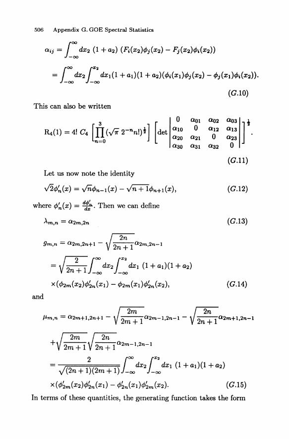
roo r'l = J -00 dx2 J -00 dXI (1 + ad (1 + a2)( cPi (XI)cPj (X2) - cPj(XI)cPi(X2))'
(G.lO)
This can also be written
R..,(l) = 41 c.lu (v;r 2-n nl)'] [det
0 (tOI (t02 (t03 r (tIO 0 (t12 (t13
(t20 (t21 0 (t23
(t30 (t31 (t32 0
(G.11)
Let us now note the identity
(G.12)
d,p' where cP~(x) = 7:"' Then we can define
(G.13)
~ 9m,n = (t2m,2n+1 - V ~(t2m,2n-1
(G.14)
and
~ ~ j..Lm,n = (t2m+I,2n+1 - V ~(t2m-I,2n-1 - V ~(t2m+I,2n-1
~~ +y ~y ~(t2m-I,2n-1
2 100 13:2 = dX2 dXI (1 + al)(l + a2) J(2n + 1)(2m + 1) -00 -00
x(cP~m(x2)cP~n(xd - cP~n(xdcP~m(X2)' (G.15)
In terms of these quantities, the generating function takes the form
G.t. The Generating FWlction R.(t) 507
R.(l) ~ 41 C.lQ, (v;r 2-n nl)t 1 [ 0 900 AOI 901 r xdet -900 0 -910 J..LOI (G.16)
AlO 910 0 911
-901 J..L10 -911 0
which has a quaternion structure. For the special case when a(xi) = a( -Xi), one can show that
J..Lij = 0 and Aij = O. For the special case when ai = 0 for all i, we find
Amn = J..Lmn = 0 and 9mn = /82 8 16mn. J' , V2n+!' t
Since [R4 (1)]{a.=0} = 1, we obtain
(G.17)
eMathematical Identities It is useful at this point to introduce some identities. Let us first note that
N-l [N-l ] TJ= !! (-Ii 2-nn!)~ = 2-N (N-l)/4 7rN/4 !! (n!)!
However,
m-l
= II [«2j + 1)7r)t r(2j + 1)] j=O
(G.18)
(G.19)
But ~r(2j + 1) = 22j r(j + ~)r(j + 1). Note also that nj:-~/2! =
23N /4. Combining these results, we find
(G.20)
508 Appendix G. GOE Spectral Statistics
Finally, let us note that nj:"(/[r(j + !)r(j + 1)] = n!:\[ir(1 + ~)] = ~n~:\r(1 + ~). Thus, we finally obtain
_ 23N /2 [m-l 2j + 1) ] N ( k) fJ - N! P ( 8 )i II r 1 + 2 .
,=0 k=l
This can be used to simplify Eq. (G .17) •
Combining Eqs. (G.17)-(G.21), we find
and the generating function, ~ (1), can be written
R.(I) = [J]<2i ; I»! J[det
0 900 AOl -900 0 -910 AlO 910 0
-901 J.L1O -911
G.2 General Case RN(l)
(G.21)
(G.22)
901 r J.LOI 911 0
(G.23)
The above expression for ~(1) can be generalized to RN(1). Explicit proofs for each step are given in [Mehta 1967]. We obtain the following quaternion form for RN(l)
1 ! 9ij J.Lij . . L,=o ..... m-l
(G.24)
For the special case a(xi) = a( -Xi) we have Aij = 0 and J.Lij = 0 and we can write Eq. (G.24) in the form
[m-l 2j + 1) 1.]
RN(l) = P ( 8 )2 detI9ijli.j=0 •...• m-l. ,=0
(G.25)
Let us now note that the matrix elements, 9ij, Aij, and J.Lij can be written in the form

G.2. General Case RN(l) 509
(G.26)
where the function, f(X), is defined f(X) = 1 for X> 0 and f(X) = -1 for x < 0;
gij = J 2j ~ 1 (Oi,j + Vij) , (G.27.a)
where
(G.27.b)
and
J1.ij = J 2i : 1 J 2j ~ 1 Pij, (G.28.a)
where
x [c/>~i(1)c/>~j(2) - c/>~;(1)c/>~i(2)]. (G.28.b)
Then the generating function takes the fonn
RN(l) = [det I fAij Oi,j + fVij I l! .(G.29) -(OJ.i + €Vji) fPij . '-0 -1
I,J- •...• m £=1
We have included the factor of f to give us an expansion parameter which reflects the dependence of the matrix elements on ai. The determinant, Eq. (G.29), may now be expanded in powers of f. Mehta shows [Mehta 1967] that
+,2i~O[det 0 Vii Aij Vij r -Vii 0 -Vji Pij
Aji Vji 0 Vjj -Vij pji -Vjj 0

510 Appendix G. GOE Spectral Statistics
m-l 1 m-l
= 1 + LVii + '2 L (ViiVjj - VijVji + AijPji)
i=O i,j=O
1 m-l
+6 L [ViiVjjVkk - 3 Vii(VjkVkj - AjkPjk) + 2VijVjkVki
i,j,k=O
(G.30)
The generating function, TN(l), for the cluster functions may then be written
m-l 1 m-l
TN(l) = InRN(l) = LVii - '2 L (VijVji - AijPji) + ... (G.31)
i=O j,i=O
The cluster functions may be obtained directly from Eq. (G.31) as described in Section (6.4). We shall obtain expressions for TI(X) and T2 (x, y) below.
G.3 Cluster Function T 1 {x)
An explicit expression for the generating function, TN(l) is given in Eq. (G.31). Let us now assume that N = 2m, where m is an integer. From Eqs. (604.16) and (G.31), we find
Tl(X) = ( DToo(1)) = lim ~(DVii) Dax {a=O} N-oo i=O Dax {a=O}
(G.32)
where ax = a(x). But from Eq. (G.27.b) we obtain
(G.33),
where ¢2i(X) is the orthonormal oscillator wave function defined in Eq. (GA) and the prime denotes its derivative. Combining Eqs. (G.32) and (G.33), we find
G.3. Cluster F\mctjon Tl (x) 511
T,(x) = J~= [~( ~i(X) - q,~i(X) f liz ¢"(Z)) l' (G.34)
With repeated use of the identity, y'2<P~(x) = vn<Pn-l(X) -vn + l<Pn+l (x), we can write Eq. (G.34) in the form
Now let us now obtain the value of Tl(X) in the neighborhood of x = O. Using the Christoffel-Darboux formula [Bateman 1953] [Mehta 1967] we note the following identity,
We will obtain the value of Tl(X) in the limit N~oo, x~O, y~O
such that the coordinates € = ~x and fJ = ~y remain finite. If we use the identities [Bateman 1953] [Mehta 1967]
N(N)t 1 lim (-1)2 -2 <PN(X) = ,-cos (7l'€) N --+OOjX,y--+O Y 71'
and 1
lim (-I)./f (N2 ) '4 <PN+l(X) = ~sin(7l'€)' N--+OOjX,y--+O y7l'
we find
(G.37)
The second term in Eq. (G.35) is negligible in the limit. Thus, we obtain the exact limiting result
lim T1(x):::::: V2N. N --+OOjX--+O 71'
(G.38)
512 Appenclix G. GOE Spectral Statistics
G.4 Cluster Function T 2 (x, y).
The cluster function T 2 {x, y) is most easily obtained from the generating function, Too{l). From Eqs. (6.4.16) and (G.30), it is defined
_~ 'E (611ij 611ji + 611ij 611ji _ 6>"ij 6pji _ 6>"ij 6Pji )] .(G.39) 2 i,j=O 6ax 6ay 6ay 6ax 6ax 6ay 6ay 6ax
However from Eqs. (G.25)-{G.27) we obtain
( /2~ij ) = -~f{Y - X)[4>~i{X)4>~j{Y) - 4>2i{Y)4>~j{x)], ay ax {a=O}
(GAO)
( ~>"ij) = 2 [4>2j (X) r dz 4>2i{Z) - 4>2i{X) r dz 4>2j {Z)] ax {a=O} Jo Jo
(GAl)
and
( ~ij) = -21 [4>~j{X)4>2i{X) - 4>~i{X)4>2j{X)]. vax {a=O}
(GA2)
If we combine the above results, we obtain after some algebra
X (4)2i{X)4>~i(Y) - 4>2i(Y)4>~i(X))
- [~ (chi (x )chi(Y) - 4>!.i(Y{ dz chi(Z) ) 1
x ['t.' ( chj (x)ch; (y) - ¢b(x) f dz chj(Z)) 1
G.4. Cluster Function T2(X, y). 513
{~ (.P2'(X )<1>;, (y) - <P2,(y).p!,,(X)) 1
X C~ ( <i>2J(x) f dz <i>2J(z)) -.p!,j (y) f dz <P2j(Z) ) 1 }.( G.(3)
We shall now obtain an espression for T2 (x, y) in the limit N -+
00, x -+ 0, Y -+ 0 so that the coordinates ~ = vrvx and "I = vrvy remain finite. Let us first note that
m-l N-l
L ¢2i(X)¢~i(Y) = L [¢i(X)¢i(Y) + ¢i( -X)¢i(y)J. (G,44) i=O i=O
Therefore, from Eq. (G.37) we obtain
. m-l J2N 11m L ¢2j(X)¢2j(Y) = - Q(~, "I),.
N--+OOjX,y--+O . 7r }=o (G,45)
where
(G,46)
Similarily, we can show that
lim 'f¢2j(X)¢~'(Y) = (J2N)2 aQ(~,TJ) N-+OOjX,y--+O . } 7r a .... }=o .,
(G,47)
and
m-l l Y lTi lim L ¢2j(X) dZ¢2j(Z) = d( Q(~, (). N --+OOjX,y--+O . 0 0 }=o
(G,4S)
With these expressions we can take the limit in Eq. (G.43). It is useful first to simplify the middle terms of Eq. (G.43) as is done in going from Eq. (G.34) to (G.35). Then, after considerable algebra, we obtain the following limiting expression for T2(x, y)

514 Appendix G. GOE Spectral Statistics
where €(r) = +1 for r > 0 and fer) = -1 for r < 0,
() sin(7rr) s r = ,
7rr (G.50)
and r = e - "1. The limiting value of T2(X,y), like that of T1(x), exhibits very simple behavior.
G.5 References
Bateman, H. (1953): Higher Transcendental Functions, Vol..~. edited by A. Erdelyi (McGraw-Hill, New York)
Mehta, M.L. (1967): Random Matrices and the Statistical Theory of Energy Levels (Academic Press, New York)

Appendix H COE Spectral Statistics
In this Appendix, we obtain the generating function, RN(I), and the cluster functions Tl (01) and T2(01, ( 2 ) for the circular orthogonal ensemble. We will illustrate the derivation of the generating function for the case R4(1), and then will give the results for RN(I). General proofs for the derivation of RN(I) can be found in [Mehta 1967J.
H.I Generating Function R4(1)
From Eqs. (6.4.9) and (9.3.14), the generating function, ~(1), for the Circular Orthogonal Ensemble can be written in the form
x lei94 _ ei9211ei94 _ ei9111ei93 _ ei9211ei93 _ ei9111ei92 _ ei91 I. (H.l)
Because the integrand is unchanged under permutation of indices we can rewrite the angle integrations in an angle ordered form if we also multiply by 4!, the number of permutations. We will also use the identity
lei9; _ei9k l = i-I (ei9; -ei9k)exp[-~i(Oj+Ok)J for OJ?.Ok.(H.2)
Then the generating function takes the form
516 Appendix H. COE Spectral Statistics
X8(04 - (3)8(03 - ( 2)8(02 - ( 1)8(01 + 11")
X exp [ - ~i( 01 + O2 + 03 + (4 )] (ei64 _ ei93 )
X (ei94 _ei92 )( ei94 _ei91 ) (ei93 _ei92)(ei93 _e i91 ) (ei92 _ei61 ), (H.3)
where 8(x) is the Heaviside function. Eq. (H.3) may now be written in terms of a Vandermonde determinant. Let us first introduce the notation fP(j)=eilj9;. Then ~(1) can be written
R.,(l) ~ 4! (W' c, 1: ... 1: dOl.·.dO, [g(1+ ai)]e( .. - 8,)
X8(04 - (3)8(03 - ( 2)8(02 - 0I)8(01) f-3(1) f-3(2) f-3(3) f-3(4) f-l(l) f-l(2) f-l(3) f-1(4)
xdet f1(1) f1(2) f1(3) fl(4) P(l) f3(2) P(3) P(4)
(H.4)
We next integrate over the angles 01 and 03 , Let us first introduce the notation
(H.5)
Then, after the integration, the generating function takes the form
R4(1) = 4! (i)-6 C4 l:l: d02d04 (1 + a2)(1 + a4)
X 8(11" - (4)8(04 - (2)8(02 + 11")
F-3(2) f-3(2) F-3(4) F-l(2) f-l(2) F-l(4)
xdet Fl(2) fl(2) Fl(4) F3(2) P(2) F3(4)
f-3(4) f-l(4) fl(4) , P(4)
(H.6)
where we have used the property that a multiple of a column in the determinant can be added to another column in the determinant without changing the value of the determinant.
The integrand in Eq. (H.6) is invariant under interchange of the angles O2 +-+04 • Therefore we can remove the restriction on the angle ordering provided we divide by 2!. If we expand the determinant and perform the remaining integrations, we obtain

H.2.Generating FUnction RN(I) 517
where
It is interesting to note that ap,q = -aq,p' Also
87r (ap,q){ai=O} = ip Dp+q,o.
If we square Rn(l), it takes on a very simple form
R~(l) = 4!2 (i)-12 cl detlapqlp,q=-3,-I,I,3,
where
detlapqlp,q=_3,_I,I,3
0 a-3,-1 a-3,1 a-3,3
= det a-I,-3 0 a_I,1 a-I,3 al,-3 al,-I 0 al,3 a3,-3 a3,-1 a3,1 0
(H.7)
(H.8)
(H.9)
(H.10)
(H.ll)
We can now easily find the normalization constant, C4, from Eq. (H.lD). If we set aj = 0 for aU j, and use Eq. (H.9) and the fact that R(lhai=o} = 1, we find C4 = 2-97r-2 •
H.2 Generating Function RN(l)
It is straightforward to generalize the calculation in Section (H.1) to the case of arbitrary N [Mehta 1967]. For simplicity we will write the results for the case of even N. The generating function, R~(l), can be written
(H.12)

518 Appendix H. COE Spectral Statistics
where N = 2m. We can now easily find the nonnalization constant, eN. If we set ai = 0 for all i in Eq. (H.12), then R~(lha.=O} = 1. This fact, together with Eq. (H.9) gives
1 eN = 22N7rf(~)t" (H.13)
Let us use Eqs. (H.9) and (H.13) to simplify Eq. (H.12). If we reverse the order of the columns in the determinant, detlapql, and use the expression for eN obtained in Eq. (H.13), we can write
R~(1) = detl,Bpqlp.q=-2m+1.-2m+3 •...• 2m-lt (H.14)
where
(H.15)
Note that ,Bpq(ai = 0) = 6p•q. If we now expand the integrand in Eq. (H.15), we can write Eq. (H.14) in the fonn
R~(I) = detl6p •q + Tpq lp •q=-2m+1.-2m+3 •...• 2m-l,
where
(H.16)
(H.17)
The generating function is now in a fonn which will enable us to obtain the cluster functions.

The cluster functions, Tn{OI, ... ,On), are defined in Eq. (6.4.16). Let us first expand the detenninant in Eq. (H.16) in powers of rpq. To second order, we find
2m-l I I R1.r{l) = 1 + L rpp + Ldet ~pp ~pq + ... ,
p=-2m+l p<q qp qq (H.18)
where the sum over p is over all integers from -2m + 1 to 2m - 1. Let us now take the logarithm of Eq. (H.18). Then we find
1 [ 2m-l TN{l) = InRN{l) = 2 L rpp - Lrpqrqp
p=-2m+l p<q
1 2m-l 2 ]
-2 L rpp+'" p=-2m+l
1 2m-l 1 2m-l 2m-l
= 2 L rpp - 4 L L rpqrqp + ... -2m+l p=-2m+lq=-2m+l
(H.19)
If we use the expression for rpq given in Eq. (H.17) and keep terms to second order in ai, we obtain
Nj'lf RN(l) = 211" -'If dJJ a(O)
xa{(1)a{02)e!Cp-q)(8 1 -82 ), (H.20)
where £(01 - (2) = e(OI - (2) - e(02 - ( 1). The cluster function, Tl (0), is just the density of levels, p(O), and
is given by
(H.21)
520 Appendix H. COE Spectral Statistics
Thus for COE, the levels have a constant density and no unfolding is necessary. The level spacing for COE is D = ~.
The cluster function, T2{'h, fh), is given by
1 (6"2TN{1») T2{lh,92 ) = 21 6" 6"
• a1 a2 {1l.=0}
2m-1 . = _ '" 1.p e{91 _ 92) eifC81-82)
L- 1611" p=-2m+1
-S!2 2~1 2~1 (1+ E)(1+!l-)e!CP-Q)C81 -82). p=-2m+1q=-2m+1 q p
Let us now introduce the function
8m(9) = 2- 2I:1 eii(8) = sin{m9) . 21r p=-2m+1 21rsin{9/2)
Then
1 ) (d8m{Ll9») { ( »2 T2{91,92) = -"2e{Ll9 dLl9 - 8m Ll9
+ ( d8j~9») fo~8 dLlfJ' 8m (Ll9'),
where Ll9 = 91 - 92. Let us now take the limit N--+oo. We define
lim (2N1r)2T2{91,92) = Y2{r), N-+oo
(H.22)
(H.23)
(H.24)
(H.25)
where r = lim (~)(91-92). Then from Eqs. (H.24) and (H.25) we N-+oo
find
Y2{r) = -!e{r) d8{r) _ (8{r»2 + d8{r) r dr' 8{r'), (H.26) 2 r r 10
where
8{r) = lim (N) 8m{91 _ 92) = sin{1rr) . N -+00 21r 1rr
(H.27)
Thus, the correlation function, Y2{r), is the same for both GOE and COE and the spectral statistics which are determined by Y2{r) are the same for the two random matrix ensembles in this limit.

H.4. References 521
H.4 References
Mehta, M.L. (1967): Random Matrices and the Statistical Theory of Energy Levels (Academic Press, New York)

Appendix I Lloyd's Model
The Lloyd's model [Lloyd 1969] is a tightbinding model of an electron on a one dimensional disordered lattice with nearest neighbor coupling. It is one of the simplest lattice models for which the electron wave function exhibits Anderson localization. In this appendix we shall derive and expression for the localization length of the electron using the Lloyd model.
1.1 Localization Length
The a th stationary state, Iua ), of the electron is determined by the Schrodinger equation, .iflua ) = ealua ), where .if is the electron Hamiltonian and ea is the energy of the electron in the a th eigenstate. Let us assume that the lattice has N lattice sites and that ua,n = (nlua ) is the probability amplitude to find the electron on the nth lattice site when the electron is in the a th eigenstate. The Schrodinger equation can be written
N
LHm,nua,n = Tmua,m + V(ua,m+1 + ua,m-t) = eaua,m, (I.1) n=l
where V is the coupling constant and Tn is the energy of the electron on the nth site. The Hamiltonian matrix is Hm n = Tnom n + , , V(Om,n+1 +Om,n-l). We will assume that eigenstates are normalized
to one, L:~=lU~,nUa,n = 1, and that the lattice is open ended so that ua,o = U a ,N+l = o. In Lloyd's model, the coupling constant, V is assumed constant and the energy, Tn, is randomly distributed. If the eigenstates on this lattice are localized, then we expect that U~,l Ua,N 'V Ae-'"('" N where A is a constant and la is the localization

1.1. Localization Length 523
length. In the remainder of this Appendix, we shall determine the average localization length,
< lOt. >= 100 ••• 100 Dr lOt. peT!, ... , TN),
-00 -00
(/.2)
where DT = dT1dT2x ... xdTN and P(Tb ... , TN) is the joint probability to find the lattice with energies, Tn, in the intervals Tl-+Tl + dTb T2-+T2 + dT2, ... , TN-+TN + dTN. In Lloyd's model, the energies, Tn, are assumed to be independent of one another so that peT!, ... , TN) = P(T1)P(T2)x ... xP(TN), and P(Tn) is chosen to be of the form
(1.3)
The first step in computing < 'YOt. > is to find an explicit expression for lOt. in terms of Tn and in a form for which we can do the integral in Eq. (1.2). We will follow a method due to Thouless [Thouless 1972] and follow a derivation given in [Haake 1990]. We repeat it here for completeness.
Let us first note that the Greens function for this system is G(z) = (zl- [I)-I, where z = e + if (cf. Sect. (8.2». The Greens function in matrix form can be written
Gm n(z) = t u~,mUOt.,n = (_l)m-n detm,n(zl- fJ), (/.4) , 0=1 z - eOt. det(zI - H)
where detm,n(zl - fJ) is the determinant of the matrix, (zl - fJ) but with the mth row and nth column missing. The left-most term in Eq. (1.4) is just the definition of the (m, n)th matrix element of the
- - - - N inverse of the matrix (zI -H). Note that det(zI -H) = nOt.=1 (z-eOt.) and because the Hamiltonian matrix for Lloyd's model is tridiagonal, dett,N(zl- fJ) = (_V)N-l. Therefore, we can write
G () _ ~ U~,IUOt.,N _ (_V)N-l I,N z - L...t - N .
Ot.=1 Z - eOt. nOt.=1 (z - eOt.) (/.5)
If we integrate Eq. (1.5) about a contour surrounding the pole at z = eOt., we find
(1.6)

524 Appendix I. Lloyd's Model
Since U~,1ua,NI'VAe-"Y .. N, we have -'YaN +In(A) = Inlu~.1ua.NI and for large N we obtain the following expression for the localization length
1 'Ya~ N Llnlea - e,81 -lnIVI·
,8=1a (1.7)
The derivative of the localization length can be written
(1.8)
It will be useful to rewrite these expressions in terms of the Green's function.
The density of states is given by, p(x) = E:=1t5(X - e,8)' Using the density of states, the quantity, 1'a, can be written
. - .!.pl°O d p(x) 'Ya - x , N -00 ea - x
(l.9)
where P denotes principle part of the integral. We can now write this in tenns of the Greens function. Note that
N N u'" U N 1 100 ( ) TrG(z) = LL a,n a,n = L = dx~. (1.10)
a=1n=1 Z - ea a=1 Z - ea -00 z - x
If we let ea--+z in Eq. (1.9) so that 1'a--+1'(z), we can write
1 100 p(x) 1 -1'(Z) = N P dx ---=- = NRe[TrG(z)].
-00 z x (1.11)
The average differentiated localization length for Lloyd's model now takes the form
1 {OO (OO _ _ < 1'(z) >= N J-oo"'J-oo DT P(T1)x ... xP(TN) Re[TrG(z)].
(1.12)
Eq. (1.12) is still not in a fonn in which the integration can be done easily. However, we can use the so-called the replica trick to put it in Gaussian fonn and thus make the integral trivial. This we do in the next subsection.

1.1. Localization Length 525
eReplica Trick Let us first note that
1~ 1~ N ... DS exp[iST.(zf - H)·S] = II90(z),
-~ -~ 0=1
(1.13)
whereDS = dS1 x ... xdSN, sr is a row matrix, sr = (St,S2, ... ,SN), and S is a column matrix obtained by taking the transpose of sr. The function, go (z) is defined
90(z) = Vi exp [i'!:'tan-1 (e -eo)]. 23v'(e - eo )2 + f2 2 f
(1.14)
Eqs. (1.13) and (1.14) are obtained by performing a unitary transformation on the integrand to make the matrix, (zf - H)m,.,,, diagonal. Then the integration is easily done. We will introduce another useful identity,
L: ... L: DS exp[i(ST·(zf - H)·S + hT·S)]
= [gga(Z)] exp[ - ~/iT.G(z)·/il. Then,
=-lim-- ... DS . {} {} {1~ 1~ -h-+O {}hm {}hn _~ _~
(1.15)
xexp[iW·(zl - B)·S + /iT ·5)] } = ~Gm •• (Z) [g ga(z) l (1.16)
If we combine the above results we can write
(1.17)

526 Appendix 1. Lloyd's Model
where SpT denotes the row vector (Sf, ... , S~) and p is an index not a power. If we take the limit, k-O in Eq. (1.17), we obtain
. k lCX> lCX> Gm,n(z) = --2~ lim IT ... DSP S~S!
k-+O p=l -CX> -CX> - T - - -
xexp[iSP ·(zl - H)·SP]. (/.18)
The Greens function is now in a form where its average may easily be taken.
Let us now take the average
Since
l CX> dTn P(Tn)e-iS?Tn = e-S?, -CX>
(1.20)
we easily find
. k lCX> lCX> < Gm,n(z) >= --2~ lim IT ... DSP S~S! k-+O 1 -00 -00 P=
- T - - -xexp[iSP ·(zl - F)·SP], (1.21)
where the matrix F has matrix elements
Fm,n = -iom,n + V(Om,n+l + Om,n-l). (1.22)
Thus, the effect of taking the average is to replace fI by F. Therefore,
(/.23)
and
1 - 1 - - 1 < i'(z) >= NRe[Trr(z)] = NRe[Tr(zl - F)- ]. (1.24)
We now have to evaluate Eq. (1.24). Let us first note that
N ! det(zl- F) = Ldetmm(zl- F). m=l
(/.25)
1.1. Localization Length 527
Thus,
N --
TrT(z) = fl d~~~~~ ~~) = !In[det(zl- F)]. (1.26)
We can evaluate Eq. (1.26) by solving a difference equation. Define DN=det(zl-F). Then Dl = z+i, D2 = (z+i)2- V2, and Dn = (e+ i)Dn- 1 - V2 Dn- 2. It is fairly easy to solve this difference equation. Let Dn = yn. Then yn = (e+i)yn-l_ V2yn-2. This has two solutions
_ e + i ±V (e + i) 2 V2 y± - -2- --2- - . (1.27)
If we assume that D N = ayf. + by!,!, where a and b are constants, and if we use the boundary conditions, Do = 1 and Dl = (e + i), then we obtain
yN+l _ yN+l DN = + -
y+ -y-(1.28)
If we now combine Eqs. (1.24) and (1.28), we obtain
1 f) [(yN+I _ yN+I)] < i'(z) >= N f)zRe In + y+ _ y= . (1.29)
Since y+ > y_, in the limit N --+00 and for € = 0 we find
< i'(z) >= :e In(y+). (1.30)
If we now integrate Eq. (1.30) and note the integration constant in Eq. (1.7), we obtain
le+i < ,(e) >= Inly+I-lnlVl = In 2V + (1.31)
and after some algebra we obtain
1 cosh( < ,(e) » = V [J(e - 2V)2 + 1 + J(e + 2V)2 + 1]. (1.32)

528 Appendix I. IJoyd's Model
1.2 References
Haake, F. (1990): Quantum Signatures of Chaos (Springer-Verlag, Heidleberg) .
Lloyd, P. (1969): J. Phys. C21717. Thouless, D.J. (1972): J. Phys. CS 77.
Appendix J Hydrogen in Parabolic Coordinates
We are interested in the behavior of the hydrogen atom in the presence of a microwave field. When an external field is present the atom becomes elongated and it is more convenient to solve the Schrodinger equation in terms of parabolic coordinates rather than spherical ~ ordinates [Landau and Lifshitz 1977], [Bethe and Salpeter 1957].
J.1 The Schrodinger Equation
The Schrodinger equation for an electron of mass, ml, and charge, -e, coupled to a proton of mass, m2, and charge, +e, via a coulomb force and in the presence of a constant electric field, Eo, can be written
(J.1)
where fO is the permittivity constant, 'Vi (i=1,2) is the Laplacian involving coordinate, rj (i=1,2) and tP = tP(rl' rz, t) is the joint pro~ ability amplitude to find the electron at rl and the proton at rz at time, t. If we introduce the relative displacement, r = rl - rz, and the center mass displacement, R = mlrl !m2rz , the Schrodinger equation
ml m2 takes the form
530 Appendix J. Hydrogen in Parabolic Coordinates
where M = ml + m2 is the total mass, p. = :,+ma is the reduced 1 ma
mass, and IjI = ljI(r, R, t).
J.1.1 Equation for Relative Motion. We can write the total energy of the system, Etot, as Etot = E + Ecm, where Ecm is the center of mass energy and E is the energy of relative motion. From Eq. (J.2) we see that the center of mass motion and the relative motion are independent of one another so we can write the wave function as
(J.3)
Then the equation for the relative motion of the electron and proton takes the form
h2 e2 --2 '1~'tfJE(r) - -4 -'tfJE(r) - e r·Eo'tfJE(r) = E'tfJE(r), (JA)
p. ~for
where 'tfJE(r) is the probability amplitude to find the electron and proton with a relative displacement, r, and relative energy, E. It is useful at this point to introduce atomic units (a.u.). We describe them briefly below .
• Atomic Units Atomic units express units of length, energy, etc. in terms of properties of the hydrogen atom assuming infinite proton mass [Bethe and Salpeter 1957]. We will here express atomic units in terms of SI units (note that the permittivity constant is fO· -
8.85434x 1O-12C2 IN.m2 and we let K.o = 1/4~fO):
1. Unit of action and of angular momentum = h= 1.05457 x 10⁻³⁴ J·s.
2. Unit of charge = e = charge of electron = 1.60218x 10⁻¹⁹ C. 3. Unit of mass = m = mass of electron = 9.10940xlO-31 kg. 4. Unit of length = aB = radius of first Bohr orbit = h2 I K.ome2 =
5.2917x 10⁻¹¹ m. 5. Unit of energy = EB = twice the ionization energy = K.~me4 Ih2
=4.3597xlO-18 J. 6. Unit of velocity = VB = electron velocity in first Bohr orbit =
K.oe2/h=2.1877x106 m/s. 7. Unit of momentum = PB = mVB = K.ome2 /h=1.9928xl0-24
kg·m/s. 8. Unit of time = tB = aBlvB = h3 IK.~me4=2A189xlO-17 s. 9. Unit offrequency = fB = vBlaB = K.~me4Ih3_4.1341xl016s-1.

J.1. The Schrodinger Equation 531
10. Unit offorce/charge = FB = l\:oe/a~=5.1422x1011 V /m.
We will assume that the electric field is directed along the z-axis so that Eo = Eoz. Then the electron and proton will be stretched apart along the z-direction and the hydrogen atom will be elongated along the z axis. In such a case, it is more natural to solve the Schrodinger equation in terms of parabolic coordinates rather than the usual spherical coordinates. We can define dimensionless parabolic coordinates, (e,.,." ¢), as follows: x = aB~ cos(¢), y = aB~ sin(¢), z = ~(e - .,.,)aB, and r = ~(e + .,.,)aB, where x, y, and z are the usual cartesian coordinates and r2 = x 2 + y2 + z2. The parabolic coordinates have a range O~e:::;oo, O~.,.,~oo and 0~¢~27r. The differential element of length, ds, in terms of dimensionless parabolic coordinates can be written
The differential element of volume can be written, dr = a1He + .,.,)d€d.,.,dl/J. The Laplacian can be written
Thus, in terms of atomic units and parabolic coordinates, the Schrodinger equation takes the form
(J.5)
where 'l/Je = 'l/Je(e,"I, ¢). We see that the Schrodinger equation de-pends on two quantities, the energy, €, and the applied force, Ao.
Eq. (J.5) can be solved by separation of variables. In Eq. (J.5), let
(J.6)
where m is the azimuthal quantum number and takes integer values to ensure that 'l/Je(e,"I,¢) is single valued on the interval 0~¢~27r. Also, multiply Eq. (J.5) by He + "I). Then Eq. (J.5) separates into two ordinary differential equations
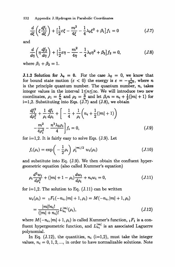
532 Appendix J. Hydrogen in Parabolic Coordinates
d ( dft ) [ 1 m2 1 2 ] - e- + -ee - - - --Xoe + fh It = 0 de de 2 4e 4 (J.7)
and
.!!:.- ('f/ dh ) + [!e'f/ - m2 - !.\0'f/2 + .B2]h = 0,
d'f/ d'f/ 2 4'f/ 4 (J.B)
where .Bl + .B2 = 1.
J.1.2 Solution for Ao = O. For the case .\0 = 0, we know that for bound state motion (e < 0) the energy is e = -~, where n is the principle quantum number. The quantum number, n, takes integer values in the interval l~n~oo. We will introduce two new coordinates, PI = ~ and P2 = ; and let .Bin = ni + ~(Iml + 1) for i=I,2. Substituting into Eqs. (J.7) and (J.B), we obtain
dJl + ~ d/i + [_! + ~ (ni + !(Iml + 1») dpr Pi dPi 4 Pi 2
_ m 2 _ n3 -XOPi ]f' = 0
4pr 4 I , (J.g)
for i=I,2. It is fairly easy to solve Eqs. (J.g). Let
/i(Pi) = exp ( - %Pi) p~m1/2 Wi(Pi) (J.I0)
and substitute into Eq. (J.g). We then obtain the confluent hypergeometric equation (also called Kummer's equation)
for i=I,2. The solution to Eq. (J.n) can be written
Wi(Pi) = IFI (-ni, Iml + 1, pd = M( -ni, Iml + 1, Pi)
= Iml!ni! Llml(-) (lml + ni)! n, P"
(J.ll)
(J.12)
where M( -ni, Iml + 1, Pi) is called Kummer's function, IFI is a confluent hypergeometric function, and Lh71 is an associated Laguerre polynomial.
In Eq. (J.12), the quantities, ni (i=I,2), must take the integer values, ni = 0, 1,2, ... , in order to have normalizable solutions. Note

J.1. The Schroclinger Equation 533
that since /31 + /32 = ~(nl + !(Iml + 1» + ~(n2 + !(lml + 1» = 1, we obtain for the principle quantum number,
n = nl +n2 + Iml + 1, (J.13)
where O~lml~n -1, O~ni~(n -Iml- 1), and m = ±Iml. If we now combine Eqs. (J.6), (J.10), and (J.12), we obtain
'l/Jnl,n'J,m(e,.",4» = c (e.,,)lml/2 e-(H'7)/2n
x Llml (i) Llml (!l.) eim4J nl n n'J n ' (J.14)
where C is a normalization constant. If we require that
~1°O de 100 d." 121r d¢ (e + .")I'l/Jnlln'J,m(e,.,,, ¢)12 = 1 (J.15)
and note that
100 dx e-X xlml (L~ml(x)) 2 = (n +nl!ml)! (J.16)
and
l°Odxe-x xlml+1 (L~ml(x»)2 = (n+nl!ml)!(2n+ lml+1),(J.17)
then we find , , C 2 _ nl·n2·
- 1rn4n2lml(lml + nl)!(lml + n2)!· (J.18)
Thus, the orthonormal eigenstates of electron-proton relative motion in parabolic coordinates are given by
e-(H'7)/2n Llml (i) Llml (!l.) eim4J. nl n n2 n (J.19)
The bound state energy is given by
-1 -1 E = - = -:-:----~_:____:_:_;:_
n2 2(nl + n2 + Iml + 1)2· (J.20)
The eigenstates in Eq. (J.19) are the most convenient to use when studying properties of the hydrogen atom in the presence of a microwave field.

534 Appendix J. Hydrogen in Parabolic Coordinates
Fig. J.1. The probability distribution for an electron in the eigenstate nl = 39, n2 = m = O. [Blwnel and Smilansky 1987]
J.2 One-dimensional Hydrogen
For the case of a large enough external field, Eo, the electron orbit will be elongated far out along the z-axis. In that case, the motion is dominated by the states, nl = 0, n2 > 0, and m = 0 and the principle quantum number is simply n = n2 + 1. The wavefunction becomes
(J.21)
where k = (n2 + 1)-1 = n-1. The motion is symmetric about the z axis. The most probable value of { is { = O. Thus, x~y~O and z~ - !77. The motion, to first approximation, is one-dimensional. In Fig. (J.1) we show the probability distribution, l'l/Jnl,o,O({, 77, 4»12 for the case nl = 39, n2 = m = O. This is identical to the distribution I1/JO,n2,O({, 77, cf»12 for the case n2 = 39, nl = m = 0 except that for nl = 39, n2 = m = 0 the electron is stretched along the positive zaxis while for n2 = 39, nl = m = 0 it is stretched along the negative z-axis.
In computing of properties of microwave driven hydrogen, we must determine the dipole matrix elements
< nj 0, n2, Ol-=-Inj 0, n~, 0 > aB
J.2. One-dimensional Hydrogen 535
= ~1000 de 1000 dTJ 1027r
d¢ (e + TJ) (e - TJ) 1/Joln~lo1/Joln~,o = (_2_) k2k'2 {2(_2_)2 roo d'TI e- iCk+k')'1
k + k' 4 k + k' 10 'f
XL~~(kry)L~~(k'ry) - 1000 dry TJ2e- iCk+k')'1 L~~(kTJ)L~~(k'TJ)}' (J.22)
where we have defined < rln; nil n2, m >= 1/Jnlln~lm(r), k = (1 + n2)-1 and k' = (1 + n2)-I. The integrals in Eq. (J.22) are tedious but can be computed. We find
100 2(n' )' on~ -n2 dTJ e- iCk+k')'1 LO (kTJ)LO, (k'ry) = 2 • ° n~ n~ n2!(n2 - n2)! (k + k')
(J.23)
and
roo dry TJ2e-iCk+k')'1 LO (kTJ)LO, (k'TJ) = 2(n2)! on~-n~ 10 n~ n 2 n2!(n2 - n2)! (k + k')
x { (4 [ (n2 - n2) _ (n2 + n2 + 1)] 2
(k-k') (k+k')
4[(n2-n2+1) _ (n2 -n2)]) + (k + k')2 (k - k')2
x 2Fl(-n2,n2 + Ijn2 - n2 + Ij02)
-8 (: ~ ::) 2 [(k: k')2 - (k _\')2 ]
( n2 (n2 + 1) ) ( " 2 } x, 1 2FI -n2+1,n2+2jn2-n2+2jo) , (J.24) n2 - n2 +
where 0 = (~+~:). Expressions for these integrals can be found in different form in [Gordon 1929] and [Zheng and Reichl 1987].
It is useful to give values of the dipole matrix element in Eq. (J.22) for some special cases:
z 3 < nj 0, n -1, Ol-Inj 0, n - 1, 0>= --2n(n -1), (J.25) aB
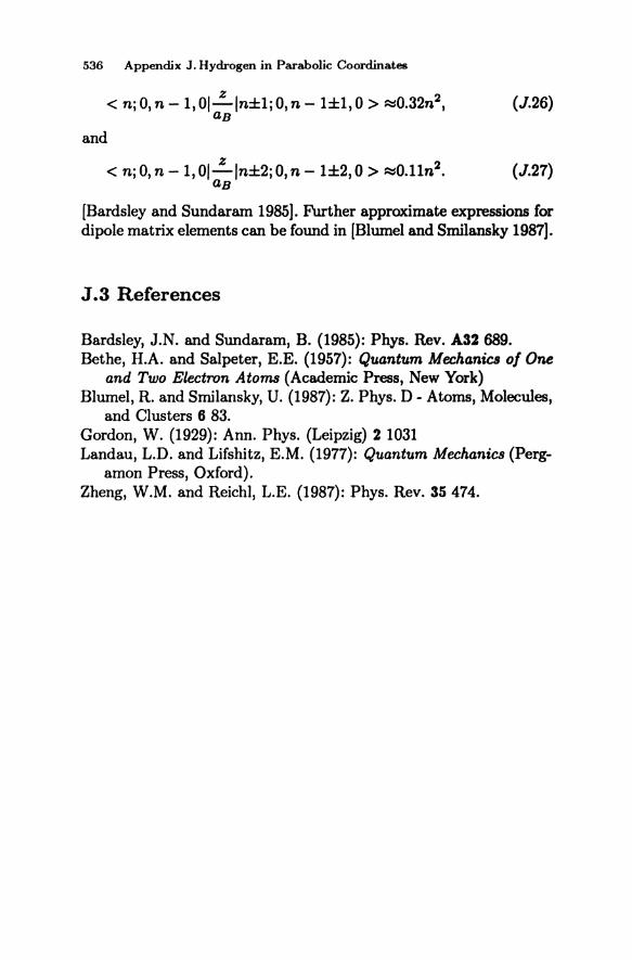
536 Appenclix J. Hydrogen jn Parabolic Coorclinates
< n;O,n -1,OI"":"'ln±I;O,n -1±1,0 > ~0.32n2, aB
and
< n; 0, n - 1, 01"":"'ln±2; 0, n - 1±2,0 > ~0.l1n2. aB
(J.26)
(J.27)
[Bardsley and Sundaram 1985]. Further approximate expressions for dipole matrix elements can be found in [Blumel and Smilansky 1987].
J.3 References
Bardsley, J.N. and Sundaram, B. (1985): Phys. Rev. A32 689. Bethe, H.A. and Salpeter, E.E. (1957): Quantum Mechanics 01 One
and Two Electron Atoms (Academic Press, New York) Blumel, R. and Smilansky, U. (1987): Z. Phys. D - Atoms, Molecules,
and Clusters 6 83. Gordon, W. (1929): Ann. Phys. (Leipzig) 2 1031 Landau, L.D. and Lifshitz, E.M. (1977): Quantum Mechanics (Perg
amon Press, Oxford). Zheng, W.M. and Reichl, L.E. (1987): Phys. Rev. 35 474.
A uthor Index
Abarbane1, H., 24, 63 Abraham, R, 5, 13,64 Antoniou, J., 153 Arfken, G., 389, 441 Arnol'd, V.I., 5, 12, 14, 15,39,43,47,
61,63,198,203,202 Atkins, P.W., 242, 247 Aubry, S., 124, 152 Avez, A., 43, 37, 61, 63 Bagley, RJ., 199-202,220 Balazs, N.L., 371, 374, 377,379 Balian, R, 264, 319, 379 Bardsley, J.N., 441, 536 Banar, R., 40, 63 Bayfield, J.E., 383, 423, 428, 436-441 Beil, J., 63 Benettin, G., 44-48, 51, 53, 63, 124,
152 Bensimon, 0.,125,152 Berman, G.P., 383, 391, 397, 405, 441 Berry, M.V., 8,12,52,63,70,72, 152,
289, 291-295, 300, 304, 313, 315, 316,320,344,347,350,354,357, 370,379
Bethe, H., 529, 530,536 Bilpuch, E.G., 316 Birkhoff, G.D., 72, 152 Bishop, A.R., 152 Bleher, S., 378, 379 Block, C., 319, 379 Blumel, R., 378, 379, 419, 420, 430,
442,535,536 Bogomolny, E.B., 370, 379 Bohigas, 0., 289, 297, 302, 303, 315,
316 Born, M., 318, 379, 463, 466 Bountis, T., 64, 115, 116, 152, 270 Bowlin, J.B., 443 Brody, T.A., 284, 286, 296, 297, 308,
312,315 Brookes, B.C., 288, 315 Brown, RC., 398, 442 Brumer, P., 368, 380 Bunimovich, L.A., 53, 63 Bums, M., 432, 433, 442
Byrd, P.F., 57, 58, 63, 208, 220, 483, 485
Camarda, H.S., 229, 315, 316 Cary, J.R, 139, 153, 154 Casartelli, M., 46, 63 Casati, G., 155, 173, 176, 177, 220,
289, 301-305, 315, 316, 354, 356, 383, 411-439, 442, 443
Cederbaum, L.S., 298, 316 Cergignani, C., 152 Channon, S.R, 133, 152 Chen, G.-Z., 154 Chen, S.-G., 154 Chen, Z.Y., 443, 445-448, 458 Cheng, Z., 289, 303, 315 Chernikov, A.A., 214-218, 220 Child, M.S., 247 Chirikov, B.V., 43, 63, 84, 113, 130-
133, 136, 137, 149, 152-155, 159, 198, 205-210, 220, 302, 315, 354, 383,413,433,442
Choquard, Ph., 318, 329, 333, 379 Cocke, S., 95, 173, 220 Collet, P., 114, 153 Cordery, R., 440, 443 Cornfeld, I.P., 415, 442 Coullet, P., 124 155 Collrant, R., 273, 286 Crawford, J.D., 154 Date, E., 25, 63 Davis, H.T., 54, 63 Delande, D., 377, 379 Delos, J.B., 377, 379 Dermott, S.F., 212, 220 Devaney, R.L., 365, 379 de Vogelaere, R., 117, 121, 153 Diana, E., 63 Dietz, B., 316 Dick, W.F.L., 288, 315 Doveil, F., 8, 12, 157, 178, 190, 191,
196,219,220,397-399,481,485 Du, M.L., 377,379 Duffing, G., 54, 63 Dunning, F.B., 443 Dyson, F.J., 248, 253, 263,265, 277,

538 Author Index
286,382,387,390,442 Eckhardt, B., 222, 247, 377-379 Ehlotzhy, F., 316 Eckmann, J.-P., 153 Einstein, A., 279, 318 Escande, D.F., 6, 12, 157, 178, 190,
191, 196, 219, 220, 397-399, 481, 485
Farquhar, I.E .. 61,63 Faulkner, R.A., 368, 379 Feigenbaum, M.J., 124, 153 Feingold, M., 314, 315,370, 379, 421,
442 Fermi, E., 149, 153 Feynman, R.P., 319, 379 Fishman, S., 383, 415, 442 Flaschka, H., 25,64 Flores, J., 286, 315 Ford, J., 25, 31, 35-38, 64, 65, 207,
209,220,442 Fornin, S.V., 442 French, J.B., 286, 315 Friedman, M.D., 57, 58, 63, 208, 220,
483,485 Friedrich, H., 376, 377,379,380 Froeshle, C., 46, 63 Galgani, L., 63, 152 Galvez, E.J., 428, 442, 443 Ganoulis, N., 223, 232, 235, 247 Gardiner, C.W., 447, 458 Gaspard, P., 294, 316, 378, 379 Gay, J.C., 377, 379 Geisel, T., 398, 399, 442 Gelfand, I.M., 329, 379 Georgopulos, P.D., 299,315 Gerasimov, A., 210, 220 Giannoni, M.J., 302, 315 Gibbons, J., 294, 316 Gilbody, H.B., 443 Ginibre, J., 454, 455, 458 Giorgilli, A., 152 Goggin, M.F., 310, 316 Gold, A., 316 Goldstein, H., 17, 19, 21, 24,64 Gordon, W., 536 Grammaticos, B., 64 Grebogi, C., 154,379 Greene, J.M., 6,12,66,80,89,92,97,
114,117,136-139,153
Grempel, D.R., 383, 415, 419, 442 Griniasti, M., 442 Grobe, R., 456-458 Guarneri, I., 155, 173, 176, 220, 301,
302,315,354,413,442 Guckenheimer, J., 81, 153 Gutzwiller, M.C., 8,12, 225, 247,316,
319,320,331,332,339,357,364, 365-368,377-380
Haake, F., 283-286, 313,316,387, 442, 454-458,523, 528
Hacken, G., 297, 316 Hagan, L., 316 Haller, E., 288, 298, 299, 316 Hamilton W.R., 3, 12 Hannay, J.H., 357, 380 Hanson, J.D., 139, 146-148, 153 Hao, B., 155, 378, 386 Haq,R.U.,297,298,316 Hardy, G.H., 96, 153 Hasagawa, H.H., 376, 380 Hasegawa, H., 133, 153, 218, 221 Hatori, T., 133, 153, 196, 220 Heiles, C., 15, 28, 30, 64 HeIleman, R., 120, 153 Heller, E.J., 320, 368-370, 380 Henon, M., 15, 25, 28, 30, 64, 133,
137, 152, 153 Hermsen, T., 294, 316 Herrera, J.C., 153, 154, 220 Hibbs, A.R., 319, 379 Hietarinta, J., 222-225, 247 Hilbert, D., 273, 286 Holmes, P.J., 81, 153, 154 Holt, C.R., 224, 225, 247 Horton, W., 153, 154, 221 Hose, G., 440, 442,443 Hua, L.K, 256, 286 Humphreys, J.E., 492, 496 Husimi, K, 374, 380 Ichikawa, Y.H., 153 Ikeda, K., 391, 443 !rie, H., 196, 220 Izrailev, F.M., 220, 383, 412, 422,
441-443 Jacobson, N., 492, 496 Jennings, B.K, 374, 379 Jensen, J.H., 488, 491 Jensen, R. V., 167, 440, 443
Jose, J.V., 440, 443 Jung, C., 378, 380 Kac, M., 25, 64 Kadanoff, L.P.,6, 97, 99-105,109,110,
125, 128, 152-155 Kamimura, T., 153 Kaneko, K, 199-202,220 Karney, C.F., 133-136, 154 Katok, A., 124, 154 Kaufman, A.N., 154, 289, 300, 301,
316 Kaufman, C., 223, 234, 242, 247, 313,
317 Kepler, J., 2,3 Kirkwood, D., 212, 220 Knox, R.S., 316 Koch, H., 153, 154 Koch, P.M., 383, 423-427, 441-443 Kolmogorov, A.N., 5, 12, 14, 15, 39,
40, 43, 64 Kolovsky, A.R., 391, 405, 441 Koppel, H., 298, 316 Kus, M., 313, 316 Lagrange, J.L., 3,13 Lambert, F., 153 Lakshmann, M., 294, 316 Landau,L.D., 168,220,463,466, 529,
536 Laplace, P.S., 2, 3 Laskar, J., 212, 213, 220 Lax, P.D., 26, 64 Lebowitz, J.L., 61, 64, 133, 152, 289,
303,315 LeDaeron, P.Y., 124, 152 Lefschetz, S., 153 Leonard, D., 454, 458 Leopold, J.G., 443 Levy, D.H., 317 Li, H., 383, 399, 400, 443 Lichtenberg, A.J.,13, 64, 81,150,154,
176, 198,220 Lieb, E., 63 Lieberman, M.A., 13,43,64,81, 150,
154, 176, 198,220 Lifshitz, E.M., 168, 220, 463, 466, 529,
536 Lighthill, J., 2, 13 Lin, W.A., 55, 64, 163, 166, 168, 193-
196, 220,391,394-397, 443
Author Index 539
Lindenberg, K, 445,458 Liou, H.I., 296, 316 Littlejohn, RG., 336, 363, 379, 380,
487,491 Liu, C., 181 Liu, J.-X., 124, 154 Louisell, W.H., 374, 380 MacKay, RS., 6, 13, 64, 67, 70, 71,
75,96,105,109-114,117,119,120, 122, 124-128, 130, 136, 139, 152.-154,220
Magyari, E., 234, 235, 247 Mansfield, P., 225, 247 Marsden, J.E., 81, 153, 154 Martin, W.C., 299, 316 Mather, J.N., 124, 154 Matsushita, T., 289, 307-310, 317 McDonald, S.W., 289, 300, 301, 316,
368,380 McKean, H.P., 318, 380 Mehta, M.L., 253, 254, 263, 273, 275,
277,283, 286,387, 443, 508, 511, 514, 515, 521
Meiss, J.D., 64, 133, 139, 143, 145, 148, 152-154, 220
Mello, P.A., 286,315 Melnikov, V.K, 67, 81, 154 Merzbacher, E., 322, 342, 380 Messiah, A., 254, 286, 497, 502 Meyer, H.D., 46, 64 Meyer, KR, 114, 154 Meyer, S.L., 288,316 Mikeska, H.J., 294, 316 Millonas, M.M., 443, 458 Milonni, P.W., 310, 316 Mishima, N., 79, 81, 87, 155 Mitchell, G.E., 316 Month, M., 153,154,200 Montroll, E.W., 329, 380 Moorman, L., 442, 443 Morette, C., 318, 330, 380 Morosov, A.D., 81,154 Moser, J., 3, 4, 5, 13-15, 24, 39, 47,
64, 77, 100, 154, 213, 220, 245, 247
Mount, KE., 344, 379 Moyal, J.E., 486, 491 Muller, G., 223, 234, 240, 242, 247,
313,317

540 Author Index
Murray, C.D., 212, 220, 221 Nakamura, K., 294, 316 Natenzon, M.Ya., 220 Newell, w.a, 443 Newson, H.W., 316 Newton, I., I, 2 Nishioka, H., 315, 380, 442 Niu, Q., 488, 491 Noether, E., 4, 13, 15, 21, 64 Olive, D.I., 225, 247 Olshanetsky, M.A., 232, 247 Oppen, G.V., 443 Ornstein, D.S., 43, 61, 64 Oseledec, V.I., 43, 64 Ott, E., 139, 143, 145, 148, 154,379 Ozorio de Almeida, A.M., 357, 380 Pande~A.,286, 297,315,316 Papadopoulos, G.J., 330, 380 Pechukas, P., 294, 316 Pehling, J.S., 379 Penrose, 0., 47, 61, 64 Percival, I.C., 124, 154,287,300,316 Pereira, N.R., 481, 485 Perelomov, A.M., 232, 247 Peres, A., 223, 232, 247, 314-316 Petrosky, T.Y., 81, 150, 154,218, 221 Petrovichev, B.A., 220 Phillips, C.S.G., 247 Piesin, Ya.G., 51, 64 Pinnaduwage, L.A., 423, 428, 441 Piro, 0., 379 Poincare, H., 4 Porter, C.E., 254, 258, 263, 264, 273,
285,286 Prange, R.E., 383, 399, 415, 442, 443 Prasad, A. V., 96, 154 Prigogine, I., 218, 221 Prochnow, N.H., 296, 316 Radons, G., 398, 399, 442, 443 Rae, J., 63 Rahn, F., 316 Rainwater, J., 316 Ramani, A., 61, 64 Ramaswamy, a, 316, 441, 443 Ramshaw, J.D., 445, 458 Rath, 0., 443 Read, F.H., 443 Rechester, A.B., 133, 154
Reichl, L.E., 22, 47, 54-61, 64, 65, 85, 153-168, 173, 193-197, 220, 221, 383, 387, 391, 394-403, 432, 433, 440, 442-445, 451, 454, 457, 458, 487,491,536
Renwick, S., 443 Rice, S.A., 316, 378, 379 Richards, D., 442, 443 Richens, P.J., 350, 380 Robnik, M., 380 Rosenbluth, M.N., 133,154 Rubner, J., 398, 442 Ruder, H., 376, 380 Sagdeev, az., 214, 220 Salpeter, E.E., 529, 536, 530 Sambe, H., 384, 443 Sanders, M.M., 438, 443 Saphir, W.C., 113, 153 Saraceno, M., 320, 369, 374, 380 Sauer,B.E., 442, 443 Scharf, a, 313, 316 Scheidecker, J.P., 46, 63 Schieve, W.C., 81, 154 Schmidt, C., 302, 315, 319 Schneider, T., 152 Scholz, H-J., 378, 380 Schulman, L.S., 319, 322, 329, 331,
339,380 Scotti, A., 63 Selberg, A., 318, 377,380 Seligman, T.H., 289,303-306,315-317,
380,442 Shenker, S.J., 6, 13, 97, 99-105,109,
110, 128, 155 Shepelyanskii, D.L., 113, 136, 137, 153,
173,176,220,412,417,420,421, 430,433,442-444
Shirley, J.H., 384, 443 Simon, B., 63 Sinai, Ya.G., 43, 51, 52, 65, 442 Slagowitz, M., 316 Smalley, aE., 298, 317 Smilansky, U., 378,379, 430,442, 535,
536 Smith, A.C.H., 443, 481, 485 Sokol, D.W., 428, 436-441 Solina, S.B., 379 Sommers, H.J., 456-458
Srivastava, N., 223, 234, 237-247, 313, 317
Stark, J., 136, 153 Stein, J., 304, 317 Stebbings, RF., 443 Stockmann, H.J., 304, 317 Stoddard, D.S., 64 Stre1cyn, J.M., 53, 63 Sundaram, B., 441, 536 Susskind, S.M., 438, 443 Sussman, G.J., 212, 213, 221 Szebehely, V., 153, 154,221 Tabor, M., 330, 315, 379 Tanaka, S., 25, 63 Tasaki, S., 221 Taylor, H.S., 440, 442,443 Taylor, RD., 368, 380 Teller, E., 292, 317 Temnyykh, A.B., 220 Tennyson, J.L., 210, 211, 220, 221 Terasaka, T., 289, 307-310, 317 Thomas, H., 247 Thomas, RG., 285, 286 Thouless, J., 523, 528 Tip, A., 443 Toda, M., 5, 13, 25, 65, 391,443 Tresser, C., 124, 155 Turner, J.S., 64 Turok, N., 225, 247 Ulam, S.M., 149, 155 Usikov, D.A., 214, 220 Vals-Gris, F., 301, 315 van Vleck, J.H., 318, 380 van Kampen, N.G., 447, 458 van Leeuwen, K.A.H., 428, 443 van Moerbeke, P., 25, 64 Verbaarshot, J.J.M., 303, 305, 316,
317 Vivaldi, F., 133, 153, 155, 207, 209,
220 Vlasova, O.F., 442 von Neumann, J., 4, 13, 290, 317 Voros, A., 371, 377, 379 Walker, G.H., 31, 35-38, 65 Wang, G.-R., 154 Watson, G.N., 169,221 Weber, R., 247 Werbin, R, 316 Weyl, H., 487, 491
Author Index 541
Wharton, L., 317 White, RB., 133, 154 Wigner, E.P., 4, 13, 248, 267, 269,
270,286,290,317,486,491 Wilkenson, M., 289, 291, 293-295, 315 Wintgen, D., 376, 377, 379, 380 Wintner, A., 20, 65 Wisdom, J., 212, 213, 221 Wong, S.S.M., 286, 315 Wright, E.M., 96, 153 Wrightman, A.S., 63 Wunner, G., 376, 380 Wyatt, RE., 398, 442 Wynchank,S.,316 Yaglom, A.M., 329,379 Yamaguchi, Y., 79, 81, 86, 87, 155 Yukawa, T., 294, 317 Zalubas, R, 316 Zaslavsky, G.M., 149, 155, 214, 220,
222,247,383,391,441 Zeldovich, Y.B., 384, 443 Zheng, W.M., 54-60,65,85,155,162,
163, 195, 197, 221, 440, 444, 536 Zirnbauer, M.R, 305, 317 Zyczkowski, K., 285, 286
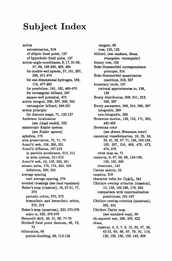
Subject Index
action extremization, 319 of elliptic fixed point, 127 of hyperbolic fixed point, 127
action-angle coordinates, 8, 17,31-38, 57,69,198-200,463,464
for double-well system, 57, 161, 207, 208, 471-474
for one-dimensional hydrogen, 169, 174,477-480
for pendulum, 181, 182, 468-470 for rectangular billiard, 347 square-well potential, 475
action integral, 336, 337, 339, 345 rectangular billiard, 348-351
action principle for discrete maps, 71, 125-127
Anderson localization (see Lloyd modeQ, 522
anisotropic Kepler system (see Kepler system)
aphelion, 175 area preservation, 70, 71, 75 Arnol'd web, 158, 200, 201 Arnol'd diffusion, 197-213
in particle accelerator, 210, 211 in solar system, 211-213
Arnol'd web, 10, 158, 200, 201 atomic units, 170, 174,424,428
definition, 530, 531 average spacing
unit average spacing, 279 avoided crossings (see level repulsion) Baker's map (classical), 16, 47-51, 77,
370 periodic orbits, 370, 372 homoclinic and heterclinic orbits,
370,374 Baker's map (quantum), 320,370-376
scars in, 320, 370-376 Bernoulli shift, 49, 51, 66, 77-79 Birkhoff fixed point theorem, 68, 72,
73 bifurcation, 68
period-doubling, 68, 113-124
tangent, 68 tree, 120, 122
billiard, (see stadium, Sinai, triangular, rectangular)
binary tree, 139 Bohr-Sommerfeld correspondence
principle, 314 Bohr-Sommerfeld quantization
condition, 318, 357 boundary circle, 137
rational approximates to, 138, 139
Brody distribution, 308, 311, 313, 346,397
Brody parameter, 309, 310, 396, 397 integrable, 289 non-integrable, 289
Brownian motion, 129, 132, 171,265, 445-458
Brownian rotor (see driven Brownian rotor)
canonical transformation, 19, 32, 34, 35,41,56,57,71,164,182-185, 192, 207, 216, 469, 470, 472, 474,476
twist map as, 71 cantorus, 9, 67, 68, 99, 124-129,
139, 195, 398 dominant, 143
Cartan matrix, 22 caustics, 319 character table for D2®S2, 242 Chirikov overlap criterion (classical),
10, 158, 162-166, 179,392 comparison with renormalization
predictions, 191-197 Chirikov overlap criterion (quantum),
392, 404 Chirikov-Taylor map
(see standard map), 86 chi-squared test, 288, 303, 422 chaos,
classical, 4, 5, 7, 9, 15, 30, 37, 38, 43-53, 60, 66, 67, 79, 91, 114, 129,133,136,139,143,308
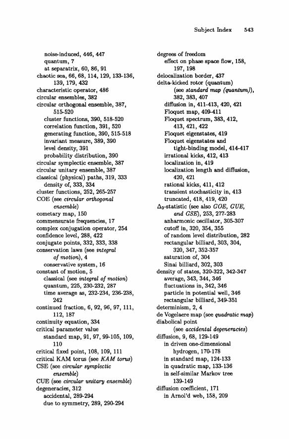
noise-induced, 446, 447 quantum, 7 at separatrix, 60, 86, 91
chaotic sea, 66, 68, 114, 129, 133-136, 139, 179, 432
characteristic operator, 486 circular ensembles, 382 circular orthogonal ensemble, 387,
515-520 cluster functions, 390, 518-520 correlation function, 391, 520 generating function, 390, 515-518 invariant measure, 389, 390 level density, 391 probability distribution, 390
circular symplectic ensemble, 387 circular unitary ensemble, 387 classical (physical) paths, 319, 333
density of, 333, 334 cluster functions, 252, 265-257 COE (see circular orthogonal
ensemble) cometary map, 150 commensurate frequencies, 17 complex conjugation operator, 254 confidence level, 288, 422 conjugate points, 332, 333, 338 conservation laws (see integral
of motion), 4 conservative system, 16
constant of motion, 5 classical (see integral of motion) quantum, 225, 230-232, 287 time average as, 232-234, 236-238,
242 continued fraction, 6, 92, 96, 97, 111,
112,187 continuity equation, 334 critical parameter value
standard map, 91, 97, 99-105, 109, 110
critical fixed point, 108, 109, 111 critical KAM torus (see KAM torus) CSE (see circular symplectic
ensemble) CUE (see circular unitary ensemble) degeneracies, 312
accidental, 289-294 due to symmetry, 289, 290-294
Subject Index 543
degrees of freedom effect on phase space flow, 158,
197, 198 delocalization border, 437 delta--kicked rotor (quantum)
(see standard map (quantum)), 382, 383, 407
diffusion in, 411-413, 420, 421 Floquet map, 409-411 Floquet spectrum, 383, 412,
413,421,422 Floquet eigenstates, 419 Floquet eigenstates and
tight-binding model, 414-417 irrational kicks, 412, 413 localization in, 419 localization length and diffusion,
420,421 rational kicks, 411, 412 transient stochasticity in, 413 truncated, 418, 419, 420
~3-statistic (see also COE, CUE, and CSE), 253, 277-283
anharmonic oscillator, 305-307 cutoff in, 320, 354,355 of random level distribution, 282 rectangular billiard, 303, 304,
320, 347, 352-357 saturation of, 304 Sinai billiard, 302, 303
density of states, 320-322, 342-347 aver'age, 343, 344, 346 fluctuations in, 342, 346 particle in potential well, 346 rectangular billiard, 349-351
determinism, 2, 4 de Vogelaere map (see quadratic map) diabolical point
(see accidental degeneracies) diffusion, 9, 68, 129-149
in driven one-dimensional hydrogen, 170-178
in standard map, 124-133 in quadratic map, 133-136 in self-similar Markov tree
139-149 diffusion coefficient, 171
in Arnol'd web, 158, 209

544 Subject Index
in driven one-dimensional hydrogen, 173, 178
in standard map, 132 and localization, 420, 421, 435, 436
diophantine approximation, 92 discrete transformation
parity, 501 time reversal, 501, 502
dissipative maps, 79 124 divergences (see perturbation theory) dominant symmetry line
(see symmetry line) double well system, 471-474 driven Brownian rotor, 445-457
diffusion in, 446 Floquet transition matrix, 452-454 Fokker-Planck equation, 447-449 Langevin equation, 445, 446 Lyapounov exponents, 446, 447 mean first passage time, 449-451 spectral statistics, 454, 456, 457
driven one-dimensional hydrogen (classical), 157, 167-178
diffusion in, 433-435 diffusion coefficient, 434
driven one-dimensional hydrogen (quantum), 428-430
continuum, 429, 430 diffusion in, 435 localization in, 433-438 pendulum approximation, 430 resonances, 430-433
Duffing map, 79 Duffing system, 16,54-60, 67, 76,
84-87, 156, 157, 161-166 dynamic Anderson localization, 8, 383,
440 in delta-kicked rotor, 413-418 in microwave-driven hydrogen, 433,
437 in one-dimensional hydrogen,
433-439 eigencurve, 74-77, 79, 81-84 electron-proton system (see hydrogen) energy conservation, 23 energy density correlation function,
278-281 energy eigenvalues
semi-classical values, 342
relation to classical orbits, 346 anisotropic Kepler system, 368
energy eigenvector distribution, 252, 284,285
energy level distribution cluster functions, 265-267 density, 267-269 joint probability distribution,
265 energy level spacing distribution,
249,270-277,349 for GOE (see Gaussian
Orthogonal Ensemble) for GSE (see Gaussian
Symplectic Ensemble) for GUE (see Gaussian Unitary
Ensemble) eigenvalue spectrum
accidental degeneracies, 289-294
degeneracies due to symmetry, 289-294
equations of motion, 294 energy surface, 197, 198
partial energy surface, 199,200 eigenvalue grid, 223, 234, 243, 244 ergodic theory, 61 extension of wavefunction
(see wave/unction) Fermi accelerator (quantum), 440
Floquet spectral statistics, 440 Fermi map, 149 Feymann path integral
(see path integral), 8, 12, 319 Fibonacci number, 97, 99, 102,
106-108 first passage time distribution
(phase space), 141, 142, 145-149
first passage time (Brownian rotor), 449-451
fixed points, 32, 43, 72, 73, 76 dominant elliptic, 106-111 elliptic, 34, 36, 56, 57, 73, SO,
91, 99-111, 115-125, 215, 218 hyperbolic, 29, 33, 36, 56, 57, 66,
73, 75-84, 88, 91, 99-111, 115-125,218
inversion hyperbolic, 75
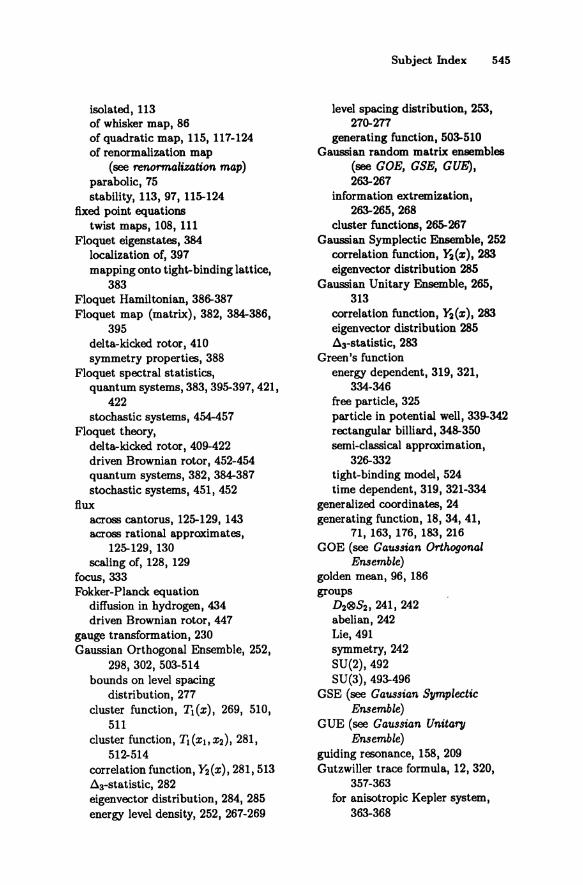
isolated, 113 of whisker map, 86 of quadratic map, 115, 117-124 of renormalization map
(see renormalization map) parabolic, 75 stability, 113, 97, 115-124
fixed point equations twist maps, 108, 111
Floquet eigenstates, 384 localization of, 397 mapping onto tight-binding lattice,
383 Floquet Hamiltonian, 386-387 Floquet map (matrix), 382, 384-386,
395 delta-kicked rotor, 410 symmetry properties, 388
Floquet spectral statistics, quantum systems, 383, 395-397, 421,
422 stochastic systems, 454-457
Floquet theory, delta-kicked rotor, 409-422 driven Brownian rotor, 452-454 quantum systems, 382, 384-387 stochastic systems, 451, 452
flux across cantorus, 125-129, 143 across rational approximates,
125-129, 130 scaling of, 128, 129
focus, 333 Fokker-Planck equation
diffusion in hydrogen, 434 driven Brownian rotor, 447
gauge transformation, 230 Gaussian Orthogonal Ensemble, 252,
298, 302, 503-514 bounds on level spacing
distribution, 277 cluster function, T1(z), 269, 510,
511 cluster function, Tl (Zit Z2), 281,
512-514 correlation function, l'2(Z) , 281, 513 d3-statistic, 282 eigenvector distribution, 284, 285 energy level density, 252, 267-269
Subject Index 545
level spacing distribution, 253, 270-277
generating function, 503-510 Gaussian random matrix ensembles
(see GOE, GSE, GUE), 263-267
information extremization, 263-265, 268
cluster functions, 265-267 Gaussian Symplectic Ensemble, 252
correlation function, l'2(z), 283 eigenvector distribution 285
Gaussian Unitary Ensemble, 265, 313
correlation function, l'2(z), 283 eigenvector distribution 285 d3-statistic, 283
Green's function energy dependent, 319, 321,
334-346 free particle, 325 particle in potential well, 339-342 rectangular billiard, 348-350 semi-classical approximation,
326-332 tight-binding model, 524 time dependent, 319, 321-334
generalized coordinates, 24 generating function, 18, 34, 41,
71,163,176,183,216 GOE (see Gaussian Orthogonal
Ensemble) golden mean, 96,186 groups
D2®S2, 241, 242 abelian, 242 Lie, 491 symmetry, 242 SU(2),492 SU(3),493-496
GSE (see Gaussian Symplectic Ensemble)
GUE (see Gaussian Unitary Ensemble)
guiding resonance, 158,209 Gutzwiller trace formula, 12, 320,
357-363 for anisotropic Kepler system,
363-368

546 Subject Index
Hamiltonian anharmonic oscillator, 305 anisotropic Kepler system, 363,
364,366 Arnol'd, 203 coupled Morse oscillators, 307 coupled standard maps, 199, 200 coupled oscillator, 207 delta-kicked harmonic oscillator, 214 delta-kicked rotor, 159,408 diamagnetic hydrogen, 376 doubl~resonance,37,342
double well system, 55, 207 driven squar~well, 166 driven on~dimensional hydrogen,
167,170 Duffing, 55, 84, 86, 161 general spin system, 235 Henon-Heiles system, 28 Holt, 224 Kepler system, 16 on~dimensional hydrogen, 169,477,
478 paradigm, 179, 188, 192 pendulum, 182, 467 rectangular billiard, 347 single-resonance, 31, 32, 35, 62 standard map, 198, 199 tim~dependent, 54, 382 Toda, 15, 224 XY model with exchange anisotropy,
236 XY model with single site anisotropy,
238 Hamiltonian (quantum)
on~dimensional hydrogen, 428, 429 Toda,225,226 Holt, 225 XY model with exchange anisotropy,
240 XY model with single site anisotropy,
241 Hamiltonian matrix, 253-263
effect of symmetry of structure, 253-258, 290-293
Hamilton's equations, 461 delta-kicked harmonic oscillator, 214 doubl~resonance, 37
driven on~dimensional hydrogen, 171,174
Duffing oscillator, 55 Henon-Heiles system, 29 Kepler system, 17 singl~resonance, 31, 32, 35 Toda lattice, 25, 26
Hamilton's principle function, 324, 325,32~331,336,337,465
definition of, 465 extremum of, 327 for free particle, 325 rectangular billiard, 347
hard sphere gas, 51 divergence in, 52
Henon-Heiles system, 28, 29, 45, 46, 51, 113, 158
Henon map (see quadratic map) hidden symmetries (see symmetry) Heisenberg equation, 497
Toda system, 226 heteroclinic points, 76-80 homoclinic points, 76-80 homogenei ty
time, 23 Husimi function, 374, 375 hydrogen
diamagnetic, 376, 377 microwav~driven (see
microwave-driven hydrogen) on~dimensional (see
one-dimensional hydrogen) hyperbolic fixed point (see fixed point) incommensurate frequencies, 17 infinitesimal transformations, 498
rotation, 500 space translation, 499, 500 time translation, 499
information extremization, 264, 268 integrability
classical system, 15, 20, 21-30, 61,222,224
quantum system 8, 222, 224, 225 integral of motion
isolating, 5, 20, 21, 27, 235, 236, 287
nonisolating, 20 integrated trace formula, 367, 368 invariant measure, 258
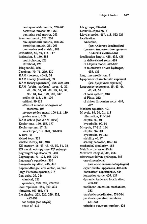
real symmetric matrix, 258-260 hermitian matrix, 261-263 quaterian real matrix, 263
invariant metric, 251, 258 real symmetric matrix, 258-260 hermitian matrix, 261-263 quaternian real matrix, 263
involution, 80, 89, 114, 117 ionization, 8, 170,383
mUlti-photon, 423 threshold,426
Ising model, 236 Jacobian, 70, 71, 259, 330 KAM theorem, 40-42, 54 KAM theory (classical), 39 KAM theory (quantum), 398,399,440 KAM (orbits, surfaces) torus, 6, 39,
42, 60, 66, 67, 68, 89, 91, 92, 96-113, 157, 179, 287, 347
noble, 96-113, 186, 190 critical, 99-113 effect of number of degrees of
freedom, 198 inverse golden mean, 100-111, 189 golden mean, 109
KAM orbits (see KAM torus) Kepler map, 150, 157, 177 Kepler system, 17,24
anisotropic, 319, 320, 364-368 K-fiow, 43 kicked tops, 313 kinetic theory, 133, 218 KS entropy, 16, 43,46, 47, 50, 51, 78 KS metric entropy (see KS entropy) Lagrange's equations, 21,460 Lagrangian, 71, 125, 168,324 Lagrange's equations, 330 Langevin equation, 445, 446 Laplace-Runge-Lenz vector, 24, 245 large Poincare systems, 218 Lax pairs, 26, 244
classical, 223 quantum, 223, 225, 227-230
level repulsion, 289, 300, 304 libration, 467-469, 471 Lie algebra, 223, 225, 229, 232,
492-494 for SU(3) (see SU(S) roots of, 495
Subject Index 547
Lie groups, 492-496 Liouville equation, 7 Lloyd's model, 417, 418, 522-527 localization
Anderson, (see Anderson localization)
dynamic Anderson (see dynamic Anderson localization)
localization length, 418, 435, 436 in delta-kicked rotor, 418 in Lloyd's model, 522-527 in microwave-driven hydrogen,
435, 436 long time prediction, 5 Lyapounov characteristic exponent
(see LyapounofJ exponent) Lyapounov exponents, 15, 43, 44,
46,47,51 of solar system, 213 of Pluto, 212 of driven Brownian rotor, 446,
447 Mathieu equation, 401 M-cycle, 89, 90, 91, 113
bifurcation, 113-124 elli ptic, 90, 91 hyperbolic, 90, 91
M,-cycle, 97-113, 124 elliptic, 97-113 hyperbolic, 97-113 stability of, 97 scaling behavior, 102-113
mechanical similarity, 168 Melnikov distance, 80-84 Melnikov integral, 205, 206 microwave-driven hydrogen, 383
one-dimensional (see one-dimensional hydrogen)
experimental apparatus, 423-426 'ionization' experiments, 424 ionization curve, 426, 427 dynamic Anderson localization,
433-438 nonlinear ionization mechanism,
383 parabolic coordinates, 531-534 parabolic quantum numbers,
531-534 principle quantum number, 424
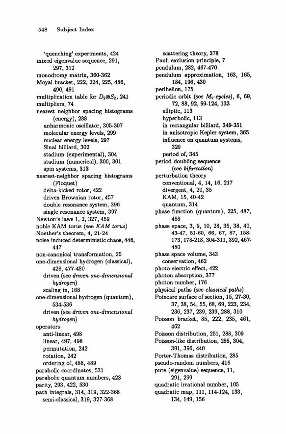
548 Subject Index
'quenching' experiments, 424 mixed eigenvalue sequence, 291,
297, 312 monodromy matrix, 360-362 Moyal bracket, 222, 224, 225,486,
490, 491 multiplication table for D2®S2, 241 multipliers, 74 nearest neighbor spacing histograms
(energy), 288 anharmonic oscillator, 305-307 molecular energy levels, 299 nuclear energy levels, 297 Sinai billiard, 302 stadium (experimental), 304 stadium (numerical), 300, 301 spin systems, 313
nearest-neighbor spacing histograms (Floquet)
delta-kicked rotor, 422 driven Brownian rotor, 457 double resonance system, 396 single resonance system, 397
Newton's laws 1, 2, 327, 459 noble KAM torus (see KAM torus) Noether's theorem, 4, 21-24 noise-induced deterministic chaos, 446,
447 non-canonical transformation, 25 on&dimensional hydrogen (classical),
428,477-480 driven (see driven one-dimensional
hydrogen) scaling in, 168
on&dimensional hydrogen (quantum), 534-536
driven (see driven one-dimensional hydrogen)
operators anti-linear, 498 linear, 497, 498 permutation, 242 rotation, 242 ordering of, 488, 489
parabolic coordinates, 531 parabolic quantum numbers, 423 parity, 293, 422, 530 path integrals, 314, 319, 322-368
semi-classical, 319, 327-368
scattering theory, 378 Pauli exclusion principle, 7 pendulum, 282, 467-470 pendulum approximation, 163, 165,
184, 196, 430 perihelion, 175 periodic orbit (see M,-cycles), 6, 69,
72, 88, 92, 99-124, 133 elliptic, 113 hyperbolic, 113 in rectangular billiard, 349-351 in anisotropic Kepler system, 365 influence on quantum systems,
320 period of, 345
period doubling sequence (see bifurcation)
perturbation theory conventional, 4, 14, 16, 217 divergent, 4, 20, 35 KAM, 15, 40-42 quantum, 314
phase function (quantum), 225, 487, 488
phase space, 3, 9, 10, 28, 35, 38, 40, 43-47, 51-60, 66, 67, 87, 158-173,178-218,304-311,392,467-480
phase space volume, 343 conservation, 462
photo-electric effect, 422 photon absorption, 377 photon number, 176 physical paths (see classical paths) Poincare surface of section, 15,27-30,
37,38,54,55,68,69,223,234, 236,237,239,239,288,310
Poisson bracket, 85, 222, 235, 461, 462
Poisson distribution, 251, 288, 309 Poisson-like distribution, 288, 304,
391, 396, 440 Porter-Thomas distribution, 285 pseudo-random numbers, 416 pure (eigenvalue) sequence, 11,
291,299 quadratic irrational number, 105 quadratic map, 111, 114-124, 133,
134, 149, 156
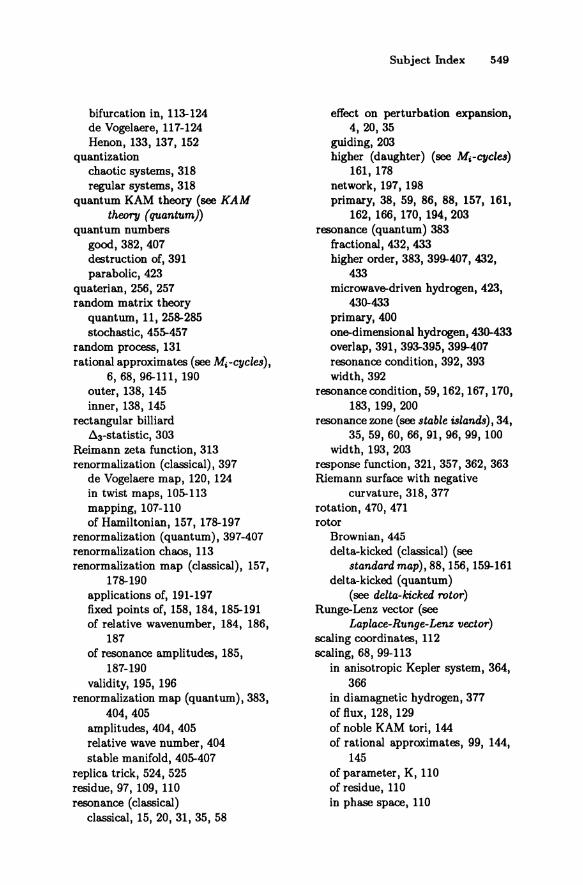
bifurcation in, 113-124 de Vogelaere, 117-124 Henon, 133, 137, 152
quantization chaotic systems, 318 regular systems, 318
quantum KAM theory (see KAM theory (quantum)
quantum numbers good, 382, 407 destruction of, 391 parabolic, 423
quaterian, 256, 257 random matrix theory
quantum, 11, 258-285 stochastic, 451).457
random process, 131 rational approximates (see Mj-cycles),
6, 68, 96-111, 190 outer, 138, 145 inner, 138, 145
rectangular billiard ~3-statistic, 303
Reimann zeta function, 313 renormalization (classical), 397
de Vogelaere map, 120, 124 in twist maps, 101).113 mapping, 107-110 of Hamiltonian, 157, 178-197
renormalization (quantum), 397-407 renormalization chaos, 113 renormalization map (classical), 157,
178-190 applications of, 191-197 fixed points of, 158, 184, 181).191 of relative wavenumber, 184, 186,
187 of resonance amplitudes, 185,
187-190 validity, 195, 196
renormalization map (quantum), 383, 404,405
amplitudes, 404, 405 relative wave number, 404 stable manifold, 401).407
replica trick, 524, 525 residue, 97, 109, 110 resonance (classical)
classical, 15, 20, 31, 35, 58
Subject Index 549
effect on perturbation expansion, 4,20,35
guiding, 203 higher (daughter) (see Mj-cycles)
161, 178 network, 197, 198 primary, 38, 59, 86, 88, 157, 161,
162,166,170,194,203 resonance (quantum) 383
fractional, 432, 433 higher order, 383, 399-407, 432,
433 microwave-driven hydrogen, 423,
430-433 primary, 400 one-dimensional hydrogen, 430-433 overlap, 391, 393-395, 399-407 resonance condition, 392, 393 width, 392
resonance condition, 59, 162, 167, 170, 183, 199, 200
resonance zone (see stable islands), 34, 35,59,60,66,91,96,99,100
width, 193, 203 response function, 321, 357, 362, 363 Riemann surface with negative
curvature, 318, 377 rotation, 470, 471 rotor
Brownian, 445 delta-kicked (classical) (see
standard map), 88,156, 159-161 delta-kicked (quantum)
(see delta-kicked rotor) Runge-Lenz vector (see
Laplace-Runge-Lenz vector) scaling coordinates, 112 scaling, 68, 99-113
in anisotropic Kepler system, 364, 366
in diamagnetic hydrogen, 377 of flux, 128, 129 of noble KAM tori, 144 of rational approximates, 99, 144,
145 of parameter, K, 110 of residue, 110 in phase space, 110
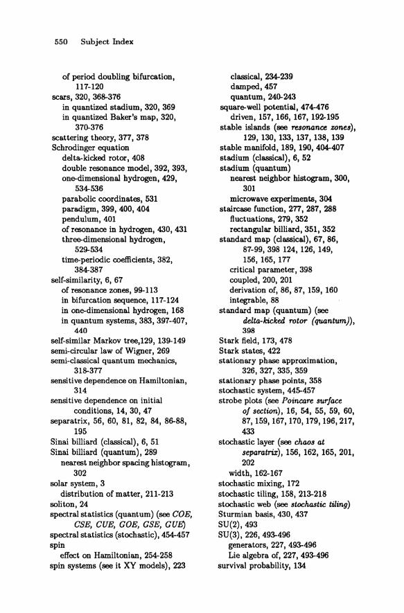
550 Subject Index
of period doubling bifurcation, 117-120
scars, 320, 368-376 in quantized stadium, 320, 369 in quantized Baker's map, 320,
370-376 scattering theory, 377, 378 Schrodinger equation
delta-kicked rotor, 408 double resonance model, 392, 393, one-dimensional hydrogen, 429,
534-536 parabolic coordinates, 531 paradigm, 399, 400,404 pendulum, 401 of resonance in hydrogen, 430,431 three-dimensional hydrogen,
529-534 time-periodic coefficients, 382,
384-387 self-similarity, 6, 67
of resonance zones, 99-113 in bifurcation sequence, 117-124 in one-dimensional hydrogen, 168 in quantum systems, 383, 397-407,
440 self-similar Markov tree,129, 139-149 semi-circular law of Wigner, 269 semi-classical quantum mechanics,
318-377 sensitive dependence on Hamiltonian,
314 sensitive dependence on initial
conditions, 14, 30, 47 separatrix, 56, 60, 81, 82, 84, 86-88,
195 Sinai billiard (classical), 6, 51 Sinai billiard (quantum), 289
nearest neighbor spacing histogram, 302
solar system, 3 distribution of matter, 211-213
soliton, 24 spectral statistics (quantum) (see COE,
eSE, CUE, COE, CSE, CUE) spectral statistics (stochastiC), 454-457 spin
effect on Hamiltonian, 254-258 spin systems (see it XY models), 223
classical, 234-239 damped,457 quantum, 240-243
square-well potential, 474-476 driven, 157, 166, 167, 192-195
stable islands (see resonance zones), 129,130,133,137,138,139
stable manifold, 189, 190, 404-407 stadium (classical), 6, 52 stadium (quantum)
nearest neighbor histogram, 300, 301
microwave experiments, 304 staircase function, 277, 287, 288
fluctuations, 279, 352 rectangular billiard, 351, 352
standard map (classical), 67, 86, 87-99, 398 124, 126, 149, 156, 165, 177
critical parameter, 398 coupled, 200, 201 derivation of, 86, 87, 159, 160 integrable, 88
standard map (quantum) (see delta-kicked rotor (quantum)), 398
Stark field, 173, 478 Stark states, 422 stationary phase approximation,
326, 327, 335, 359 stationary phase points, 358 stochastic system, 445-457 strobe plots (see Poincare surface
of section), 16, 54, 55, 59, 60, 87,159,167,170,179,196,217, 433
stochastic layer (see chaos at separatrix) , 156, 162, 165, 201, 202
width, 162-167 stochastic mixing, 172 stochastic tiling, 158, 213-218 stochastic web (see stochastic tiling) Sturmian basis, 430, 437 SU(2),493 SU(3), 226, 493-496
generators, 227, 493-496 Lie algebra of, 227, 493-496
survival probability, 134
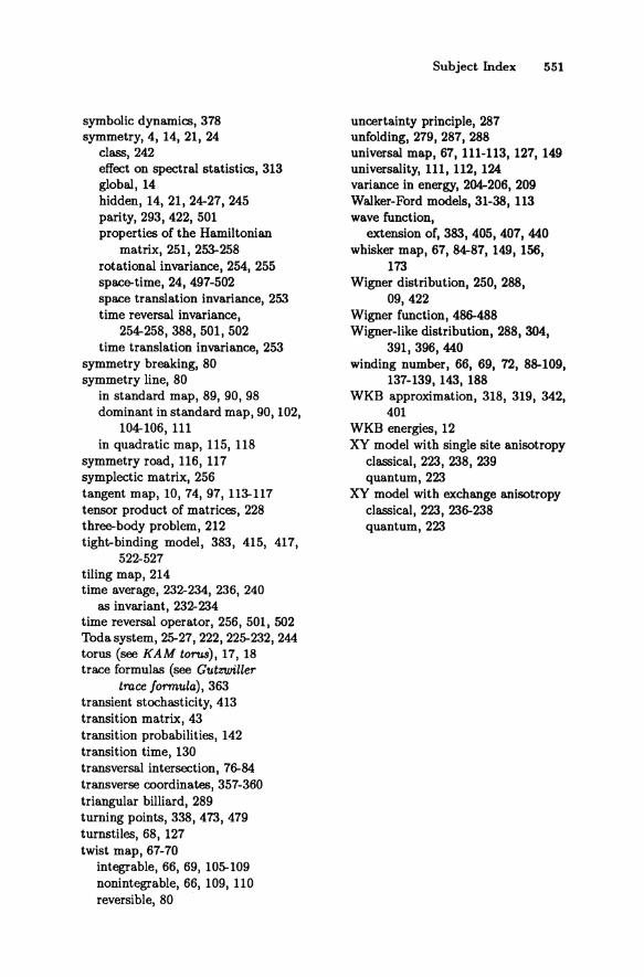
symbolic dynamics, 378 symmetry, 4, 14, 21, 24
class, 242 effect on spectral statistics, 313 global, 14 hidden, 14, 21, 24-27, 245 parity, 293,422, 501 properties of the Hamiltonian
matrix, 251, 253-258 rotational invariance, 254, 255 space-time, 24, 497-502 space translation invariance, 253 time reversal invariance,
254-258,388,501,502 time translation invariance, 253
symmetry breaking, 80 symmetry line, 80
in standard map, 89, 90, 98 dominant in standard map, 90, 102,
104-106, 111 in quadratic map, 115, 118
symmetry road, 116, 117 symplectic matrix, 256 tangent map, 10, 74, 97, 113-117 tensor product of matrices, 228 three-body problem, 212 tight-binding model, 383, 415, 417,
522-527 tiling map, 214 time average, 232-234, 236, 240
as invariant, 232-234 time reversal operator, 256, 501, 502 Toda system, 25-27, 222, 225-232, 244 torus (see KAM torus), 17, 18 trace formulas (see Gutzwiller
trace formula), 363 transient stochasticity, 413 transition matrix, 43 transition probabilities, 142 transition time, 130 transversal intersection, 76-84 transverse coordinates, 357-360 triangular billiard, 289 turning points, 338, 473, 479 turnstiles, 68, 127 twist map, 67-70
integrable, 66, 69, 105-109 nonintegrable, 66, 109, 110 reversible, 80
Subject fudex 551
uncertainty principle, 287 unfolding, 279, 287, 288 universal map, 67, 111-113, 127, 149 universality, 111, 112, 124 variance in energy, 204-206, 209 Walker-Ford models, 31-38, 113 wave function,
extension of, 383, 405, 407, 440 whisker map, 67, 84-87, 149, 156,
173 Wigner distribution, 250, 288,
09, 422 Wigner function, 486-488 Wigner-like distribution, 288, 304,
391, 396, 440 winding number, 66, 69, 72, 88-109,
137-139, 143, 188 WKB approximation, 318, 319, 342,
401 WKB energies, 12 XY model with single site anisotropy
classical, 223, 238, 239 quantum, 223
XY model with exchange anisotropy classical, 223, 236-238 quantum, 223
Related Documents


![Classical Mechanics - people.phys.ethz.chdelducav/cmscript.pdf · References [1]LandauandLifshitz,Mechanics,CourseofTheoreticalPhysicsVol.1., PergamonPress [2]Classical Mechanics,](https://static.cupdf.com/doc/110x72/5e1e9832bac1ea74484e9601/classical-mechanics-delducavcmscriptpdf-references-1landauandlifshitzmechanicscourseoftheoreticalphysicsvol1.jpg)