Final Report 86 Appendix A: Carbon Intensity Analysis WA-GREET Methodology A Washington-specific GREET model was developed by Life Cycle Associates in 2013 that was based on the Argonne National Laboratory (ANL) GREET model version GREET1_2013. ICF and the Agency agreed that this model is outdated with assumptions and data from prior to 2013. Instead of using the 2013 model, ICF recommended modifying the California Air Resources Board’s (CARB) CA-GREET3.0 model. It was agreed this would be the most relevant and expedient solution to developing a current, Washington-specific GREET model. CA-GREET3.0 is currently used for fuel pathways in California’s Low Carbon Fuel Standard (LCFS) and would allow for consistency in overall assumptions and modeling framework between a Washington model and the LCFS. The modifications of the CA-GREET3.0 to develop a WA-GREET are summarized in the following sections. Electricity Grid Mix Update ICF updated the Electricity Generation Mixes with EPA’s Emissions & Generation Resource Integrated Database (eGRID) 2016 data 103 . Since it is unlikely to be used, ICF replaced the user’s option for Hawaii HICC Miscellaneous eGRID subregion with a Washington State option. ICF replaced all HICC data with Washington State data. This includes regional combustion technology shares, regional power plant energy conversion efficiencies, and the electric generation mix of the state of Washington. 103 ICF compared the generation mix of the utilities serving the Puget Sound counties 104 with the Washington State average. Due to Puget Sound Energy’s significant use of coal generation, the carbon intensity of electricity from utilities in the four county Puget Sound region was calculated to be over two times greater than the Washington State average. Table 37 and Table 38 below provide a comparison of the electricity mixes in Puget Sound versus the Washington average. Table 37 does not include a few smaller utilities serving communities in Pierce County. Since the service areas of these utilities would only be a small fraction of the total service area in Puget Sound (less than 5%), they were excluded. They are conceptually represented by Lakeview and Peninsula. The excluded utilities are Fircrest, Milton, Elmhurst Mutual, Parkland, Ruston, and Steilacoom. 103 US EPA, Emissions and Generated Resource Integrated Database 2016. Available at: https://www.epa.gov/energy/emissions-generation-resource-integrated-database-egrid; released 2/15/2018 104 Puget Sound Clean Air Agency, Greenhouse Gas Emissions Inventory, Tables 5 & 6, 2018. Available at: http://www.pscleanair.org/DocumentCenter/View/3328/PSCAA-GHG-Emissions-Inventory

Welcome message from author
This document is posted to help you gain knowledge. Please leave a comment to let me know what you think about it! Share it to your friends and learn new things together.
Transcript
Final Report
86
Appendix A: Carbon Intensity Analysis WA-GREET Methodology A Washington-specific GREET model was developed by Life Cycle Associates in 2013 that was based on the Argonne National Laboratory (ANL) GREET model version GREET1_2013. ICF and the Agency agreed that this model is outdated with assumptions and data from prior to 2013. Instead of using the 2013 model, ICF recommended modifying the California Air Resources Board’s (CARB) CA-GREET3.0 model. It was agreed this would be the most relevant and expedient solution to developing a current, Washington-specific GREET model. CA-GREET3.0 is currently used for fuel pathways in California’s Low Carbon Fuel Standard (LCFS) and would allow for consistency in overall assumptions and modeling framework between a Washington model and the LCFS. The modifications of the CA-GREET3.0 to develop a WA-GREET are summarized in the following sections.
Electricity Grid Mix Update ICF updated the Electricity Generation Mixes with EPA’s Emissions & Generation Resource Integrated Database (eGRID) 2016 data103. Since it is unlikely to be used, ICF replaced the user’s option for Hawaii HICC Miscellaneous eGRID subregion with a Washington State option. ICF replaced all HICC data with Washington State data. This includes regional combustion technology shares, regional power plant energy conversion efficiencies, and the electric generation mix of the state of Washington.103 ICF compared the generation mix of the utilities serving the Puget Sound counties104 with the Washington State average. Due to Puget Sound Energy’s significant use of coal generation, the carbon intensity of electricity from utilities in the four county Puget Sound region was calculated to be over two times greater than the Washington State average. Table 37 and Table 38 below provide a comparison of the electricity mixes in Puget Sound versus the Washington average. Table 37 does not include a few smaller utilities serving communities in Pierce County. Since the service areas of these utilities would only be a small fraction of the total service area in Puget Sound (less than 5%), they were excluded. They are conceptually represented by Lakeview and Peninsula. The excluded utilities are Fircrest, Milton, Elmhurst Mutual, Parkland, Ruston, and Steilacoom.
103 US EPA, Emissions and Generated Resource Integrated Database 2016. Available at: https://www.epa.gov/energy/emissions-generation-resource-integrated-database-egrid; released 2/15/2018
104 Puget Sound Clean Air Agency, Greenhouse Gas Emissions Inventory, Tables 5 & 6, 2018. Available at: http://www.pscleanair.org/DocumentCenter/View/3328/PSCAA-GHG-Emissions-Inventory

Final Report
87
Table 37: Reported Fuel Mix of Electric Utilities in PSCAA Region, 2017104
Fuel Puget Sound Energy105
Seattle City106 Snohomish107 Tacoma108 Peninsula109 Lakeview110 Weighted
Average
Residual Oil/Fossil fuels 0.1% 0.0% 0.0% 0.0% 0.0% 0.0% 0%
Natural gas 21.0% 1.0% 0.4% 1.0% 1.0% 0.9% 10% Coal 38.0% 1.0% 0.4% 1.5% 1.0% 2.4% 17% Nuclear 0.6% 4.0% 9.0% 6.1% 8.0% 10.2% 4% Biomass 0.3% 1.0% 0.2% 0.2% 0.0% 0.2% 0% Hydroelectric 33.0% 91.0% 90.0% 84.0% 83.0% 86.3% 65% Geothermal 0.0% 0.0% 0.0% 0.0% 0.0% 0.0% 0% Wind 6.0% 1.0% 0.0% 7.0% 7.0% 0.0% 4% Solar PV 0.0% 0.0% 0.0% 0.0% 0.0% 0.0% 0% Others (purchased) 1.0% 1.0% 0.0% 0.2% 0.0% 0.1% 1% Proportion Based on kWh Consumed 43.58% 25.06% 17.04% 12.09% 1.54% 0.69% GREET CI [g CO2e/MJ] 150.47 4.90 2.00 6.27 4.75 8.76 68.03
Pathway CI for LD BEV111 44.3 1.44 0.59 1.84 1.40 2.58 20.0
105 Accessed via https://www.pse.com/pages/energy-supply/electric-supply 106 Accessed via http://www.seattle.gov/light/FuelMix/ 107 Accessed via https://www.snopud.com/PowerSupply.ashx?p=1105 108 Accessed via https://www.mytpu.org/tacomapower/about-tacoma-power/dams-power-sources/ 109 Accessed via https://www.penlight.org/energy-services/power-resources/ 110 Accessed via https://lakeviewlight.com/wp-content/uploads/LLP-Spring-2017-Newsletter_Final_Production-Ready.pdf
111 This is the estimated pathway for a light-duty BEV accounting for the Energy Economy Ratio (EER) of 3.4.
Final Report
88
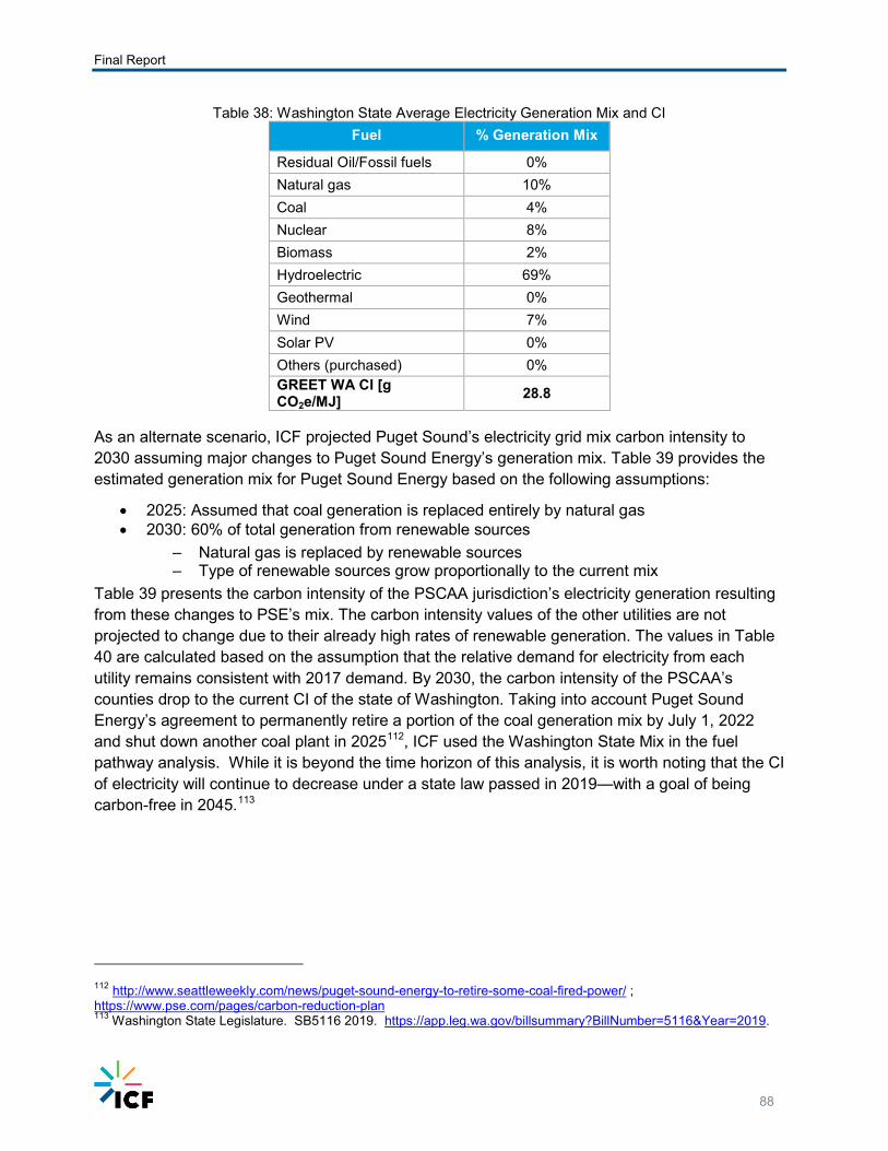
Table 38: Washington State Average Electricity Generation Mix and CI Fuel % Generation Mix
Residual Oil/Fossil fuels 0% Natural gas 10% Coal 4% Nuclear 8% Biomass 2% Hydroelectric 69% Geothermal 0% Wind 7% Solar PV 0% Others (purchased) 0% GREET WA CI [g CO2e/MJ] 28.8
As an alternate scenario, ICF projected Puget Sound’s electricity grid mix carbon intensity to 2030 assuming major changes to Puget Sound Energy’s generation mix. Table 39 provides the estimated generation mix for Puget Sound Energy based on the following assumptions:
• 2025: Assumed that coal generation is replaced entirely by natural gas • 2030: 60% of total generation from renewable sources
– Natural gas is replaced by renewable sources – Type of renewable sources grow proportionally to the current mix
Table 39 presents the carbon intensity of the PSCAA jurisdiction’s electricity generation resulting from these changes to PSE’s mix. The carbon intensity values of the other utilities are not projected to change due to their already high rates of renewable generation. The values in Table 40 are calculated based on the assumption that the relative demand for electricity from each utility remains consistent with 2017 demand. By 2030, the carbon intensity of the PSCAA’s counties drop to the current CI of the state of Washington. Taking into account Puget Sound Energy’s agreement to permanently retire a portion of the coal generation mix by July 1, 2022 and shut down another coal plant in 2025112, ICF used the Washington State Mix in the fuel pathway analysis. While it is beyond the time horizon of this analysis, it is worth noting that the CI of electricity will continue to decrease under a state law passed in 2019—with a goal of being carbon-free in 2045.113
112 http://www.seattleweekly.com/news/puget-sound-energy-to-retire-some-coal-fired-power/ ; https://www.pse.com/pages/carbon-reduction-plan 113 Washington State Legislature. SB5116 2019. https://app.leg.wa.gov/billsummary?BillNumber=5116&Year=2019.
Final Report
89
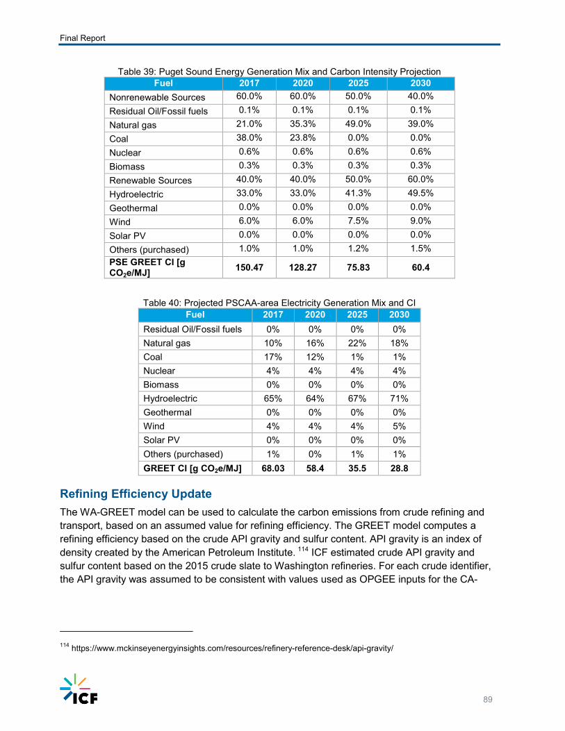
Table 39: Puget Sound Energy Generation Mix and Carbon Intensity Projection Fuel 2017 2020 2025 2030
Nonrenewable Sources 60.0% 60.0% 50.0% 40.0% Residual Oil/Fossil fuels 0.1% 0.1% 0.1% 0.1% Natural gas 21.0% 35.3% 49.0% 39.0% Coal 38.0% 23.8% 0.0% 0.0% Nuclear 0.6% 0.6% 0.6% 0.6% Biomass 0.3% 0.3% 0.3% 0.3% Renewable Sources 40.0% 40.0% 50.0% 60.0% Hydroelectric 33.0% 33.0% 41.3% 49.5% Geothermal 0.0% 0.0% 0.0% 0.0% Wind 6.0% 6.0% 7.5% 9.0% Solar PV 0.0% 0.0% 0.0% 0.0% Others (purchased) 1.0% 1.0% 1.2% 1.5% PSE GREET CI [g CO2e/MJ] 150.47 128.27 75.83 60.4
Table 40: Projected PSCAA-area Electricity Generation Mix and CI Fuel 2017 2020 2025 2030
Residual Oil/Fossil fuels 0% 0% 0% 0% Natural gas 10% 16% 22% 18% Coal 17% 12% 1% 1% Nuclear 4% 4% 4% 4% Biomass 0% 0% 0% 0% Hydroelectric 65% 64% 67% 71% Geothermal 0% 0% 0% 0% Wind 4% 4% 4% 5% Solar PV 0% 0% 0% 0% Others (purchased) 1% 0% 1% 1% GREET CI [g CO2e/MJ] 68.03 58.4 35.5 28.8
Refining Efficiency Update The WA-GREET model can be used to calculate the carbon emissions from crude refining and transport, based on an assumed value for refining efficiency. The GREET model computes a refining efficiency based on the crude API gravity and sulfur content. API gravity is an index of density created by the American Petroleum Institute. 114 ICF estimated crude API gravity and sulfur content based on the 2015 crude slate to Washington refineries. For each crude identifier, the API gravity was assumed to be consistent with values used as OPGEE inputs for the CA-
114 https://www.mckinseyenergyinsights.com/resources/refinery-reference-desk/api-gravity/
Final Report
90
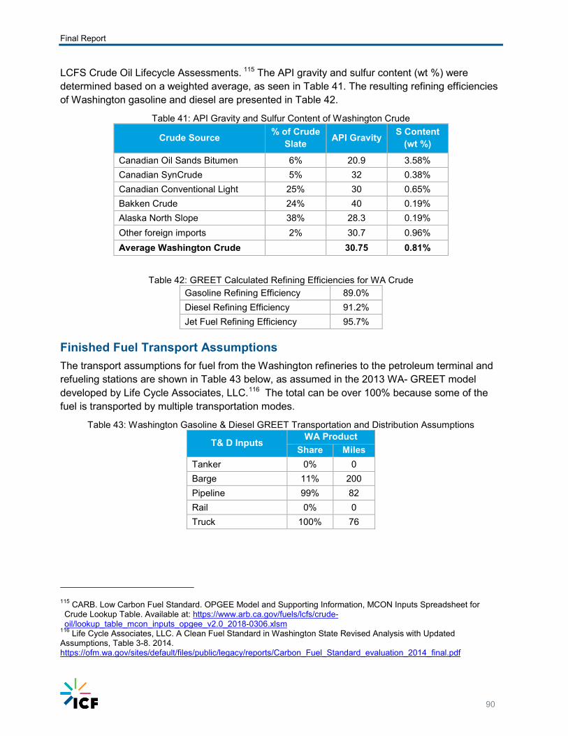
LCFS Crude Oil Lifecycle Assessments. 115 The API gravity and sulfur content (wt %) were determined based on a weighted average, as seen in Table 41. The resulting refining efficiencies of Washington gasoline and diesel are presented in Table 42.
Table 41: API Gravity and Sulfur Content of Washington Crude
Crude Source % of Crude Slate API Gravity S Content
(wt %) Canadian Oil Sands Bitumen 6% 20.9 3.58% Canadian SynCrude 5% 32 0.38% Canadian Conventional Light 25% 30 0.65% Bakken Crude 24% 40 0.19% Alaska North Slope 38% 28.3 0.19% Other foreign imports 2% 30.7 0.96% Average Washington Crude 30.75 0.81%
Table 42: GREET Calculated Refining Efficiencies for WA Crude Gasoline Refining Efficiency 89.0% Diesel Refining Efficiency 91.2% Jet Fuel Refining Efficiency 95.7%
Finished Fuel Transport Assumptions The transport assumptions for fuel from the Washington refineries to the petroleum terminal and refueling stations are shown in Table 43 below, as assumed in the 2013 WA- GREET model developed by Life Cycle Associates, LLC.116 The total can be over 100% because some of the fuel is transported by multiple transportation modes.
Table 43: Washington Gasoline & Diesel GREET Transportation and Distribution Assumptions
T& D Inputs WA Product Share Miles
Tanker 0% 0 Barge 11% 200 Pipeline 99% 82 Rail 0% 0 Truck 100% 76
115 CARB. Low Carbon Fuel Standard. OPGEE Model and Supporting Information, MCON Inputs Spreadsheet for Crude Lookup Table. Available at: https://www.arb.ca.gov/fuels/lcfs/crude-oil/lookup_table_mcon_inputs_opgee_v2.0_2018-0306.xlsm
116 Life Cycle Associates, LLC. A Clean Fuel Standard in Washington State Revised Analysis with Updated Assumptions, Table 3-8. 2014. https://ofm.wa.gov/sites/default/files/public/legacy/reports/Carbon_Fuel_Standard_evaluation_2014_final.pdf

Final Report
91
Washington Crude Carbon Intensity To calculate the upstream carbon intensity of gasoline and diesel produced in Washington, ICF utilized the OPGEE results from California’s LCFS Crude Oil Life Cycle Assessments117. ICF estimated a Washington Crude Oil Production and Transport CI by using the average LCFS reported crude carbon intensities, weighted by the proportion of each source. The upstream gasoline and diesel CI is estimated to be 12.96 g CO2e/MJ, as shown in Table 44.
Table 44: Washington Crude Oil Production and Transportation Carbon Intensity
Crude Source LCFS Crude Identifier LCFS CI [g CO2e/MJ]
Average CI
% WA Crude Slate
Canadian Oil Sands Bitumen
Christina Dilbit Blend 12.71 14.56 6%
Statoil Cheecham Dilbit 16.41
Canadian SynCrude
Albian Heavy Synthetic (all grades) 23.68
29.64 5%
CNRL Light Sweet Synthetic 25.27 Hardisty Synthetic 32.66
Long Lake Light Synthetic 40.12 Premium Albian Synthetic 29.49
Premium Synthetic 27.38 Shell Synthetic (all grades) 29.49
Suncor Synthetic (all grades) 27.09 Syncrude Synthetic (all grades) 31.62
Canadian Conventional Light Canadian Conventional Light 8.11 8.11 25%
Bakken Crude US North Dakota Bakken 9.73 9.73 24% Alaska North Slope Alaska North Slope 15.91 15.91 38% All foreign imports Weighted Average of all others 12.96 12.96 2% WA Crude Mix CI 13.13
117 CARB Low Carbon Fuel Standard Final Regulation Order, Table 9: Carbon Intensity Lookup Table for Crude Oil Production and Transport. 2018. Available at: https://www.arb.ca.gov/regact/2018/lcfs18/frolcfs.pdf?_ga=2.246951810.766619030.1548198089-546402948.1536794631
Final Report
92
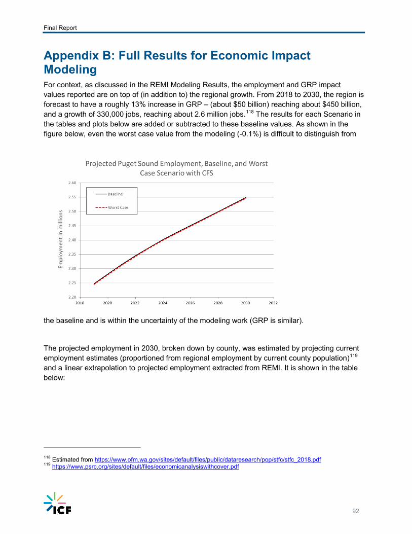
Appendix B: Full Results for Economic Impact Modeling For context, as discussed in the REMI Modeling Results, the employment and GRP impact values reported are on top of (in addition to) the regional growth. From 2018 to 2030, the region is forecast to have a roughly 13% increase in GRP – (about $50 billion) reaching about $450 billion, and a growth of 330,000 jobs, reaching about 2.6 million jobs.118 The results for each Scenario in the tables and plots below are added or subtracted to these baseline values. As shown in the figure below, even the worst case value from the modeling (-0.1%) is difficult to distinguish from
the baseline and is within the uncertainty of the modeling work (GRP is similar).
The projected employment in 2030, broken down by county, was estimated by projecting current employment estimates (proportioned from regional employment by current county population)119 and a linear extrapolation to projected employment extracted from REMI. It is shown in the table below:
118 Estimated from https://www.ofm.wa.gov/sites/default/files/public/dataresearch/pop/stfc/stfc_2018.pdf 119 https://www.psrc.org/sites/default/files/economicanalysiswithcover.pdf

Final Report
93
County 2016 2030 Projected Kitsap 151,000 180,000 Snohomish 409,000 480,000 King 1,140,000 1,350,000 Pierce 452,000 540,000 Region 2,150,000 2,550,000
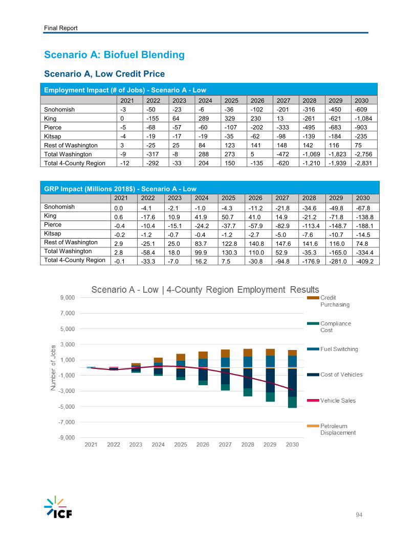
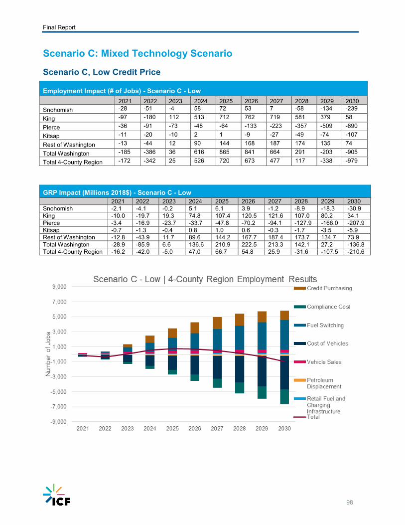
The employment impact results for each scenario are presented in a series of tables and graphs in the sub-sections below; in each figure, there are seven categories or factors that are plotted to what drives the overall trend. The table below lists the categories and provides a brief description of what each category represents.
Impact Category Description
Credit Purchasing • Reflects the increased revenue to low carbon fuel providers based on the value of
credits generated via the deployment of the lower carbon fuels in the Puget Sound region.
Compliance Cost • Accounts for the assumption that the compliance cost (i.e., purchasing credits) will be passed through to consumers.
Fuel Switching • Low carbon fuels like electricity and natural gas have a lower price than petroleum-
based fuels, yielding a lower total cost of ownership. These lower fuel costs are reflected in this category.
Cost of Vehicles
• Alternative fuel vehicles, like EVs and NGVs, tend to be more expensive than their conventional counterparts that use combustion engines. As a result, there are increased expenditures by consumers and commercial and industrial sectors that for light-duty vehicles and MD/HD vehicles, respectively. ICF assumed that EV pricing over time, but even
Vehicle Sales • The increased costs of alternative fuel vehicles also yields increased investment by
the vehicle manufacturing sector, thereby increasing economic activity in the sector and associated economic sectors.
Petroleum Displacement
• The implementation of a Puget Sound CFS will reduce the amount of petroleum consumed in the region, thereby decreased regional demand for petroleum. This will have a negative impact on the refining industry—and this category reflects the decrease in revenue to refineries as a result of either displaced product, or higher transportation costs to export the product out of the region.
Retail Fuel and Charging Infrastructure
• Low carbon fuels will require investment in new or modified retail fueling infrastructure—these investments include converting existing petroleum-based fueling infrastructure to accommodate higher biofuel blends to providing and deploying EV charging infrastructure.
Final Report
94
Scenario A: Biofuel Blending
Scenario A, Low Credit Price Employment Impact (# of Jobs) - Scenario A - Low 2021 2022 2023 2024 2025 2026 2027 2028 2029 2030 Snohomish -3 -50 -23 -6 -36 -102 -201 -316 -450 -609 King 0 -155 64 289 329 230 13 -261 -621 -1,084 Pierce -5 -68 -57 -60 -107 -202 -333 -495 -683 -903 Kitsap -4 -19 -17 -19 -35 -62 -98 -139 -184 -235 Rest of Washington 3 -25 25 84 123 141 148 142 116 75 Total Washington -9 -317 -8 288 273 5 -472 -1,069 -1,823 -2,756 Total 4-County Region -12 -292 -33 204 150 -135 -620 -1,210 -1,939 -2,831
GRP Impact (Millions 2018$) - Scenario A - Low
2021 2022 2023 2024 2025 2026 2027 2028 2029 2030 Snohomish 0.0 -4.1 -2.1 -1.0 -4.3 -11.2 -21.8 -34.6 -49.8 -67.8 King 0.6 -17.6 10.9 41.9 50.7 41.0 14.9 -21.2 -71.8 -138.8 Pierce -0.4 -10.4 -15.1 -24.2 -37.7 -57.9 -82.9 -113.4 -148.7 -188.1 Kitsap -0.2 -1.2 -0.7 -0.4 -1.2 -2.7 -5.0 -7.6 -10.7 -14.5 Rest of Washington 2.9 -25.1 25.0 83.7 122.8 140.8 147.6 141.6 116.0 74.8 Total Washington 2.8 -58.4 18.0 99.9 130.3 110.0 52.9 -35.3 -165.0 -334.4 Total 4-County Region -0.1 -33.3 -7.0 16.2 7.5 -30.8 -94.8 -176.9 -281.0 -409.2
Final Report
95
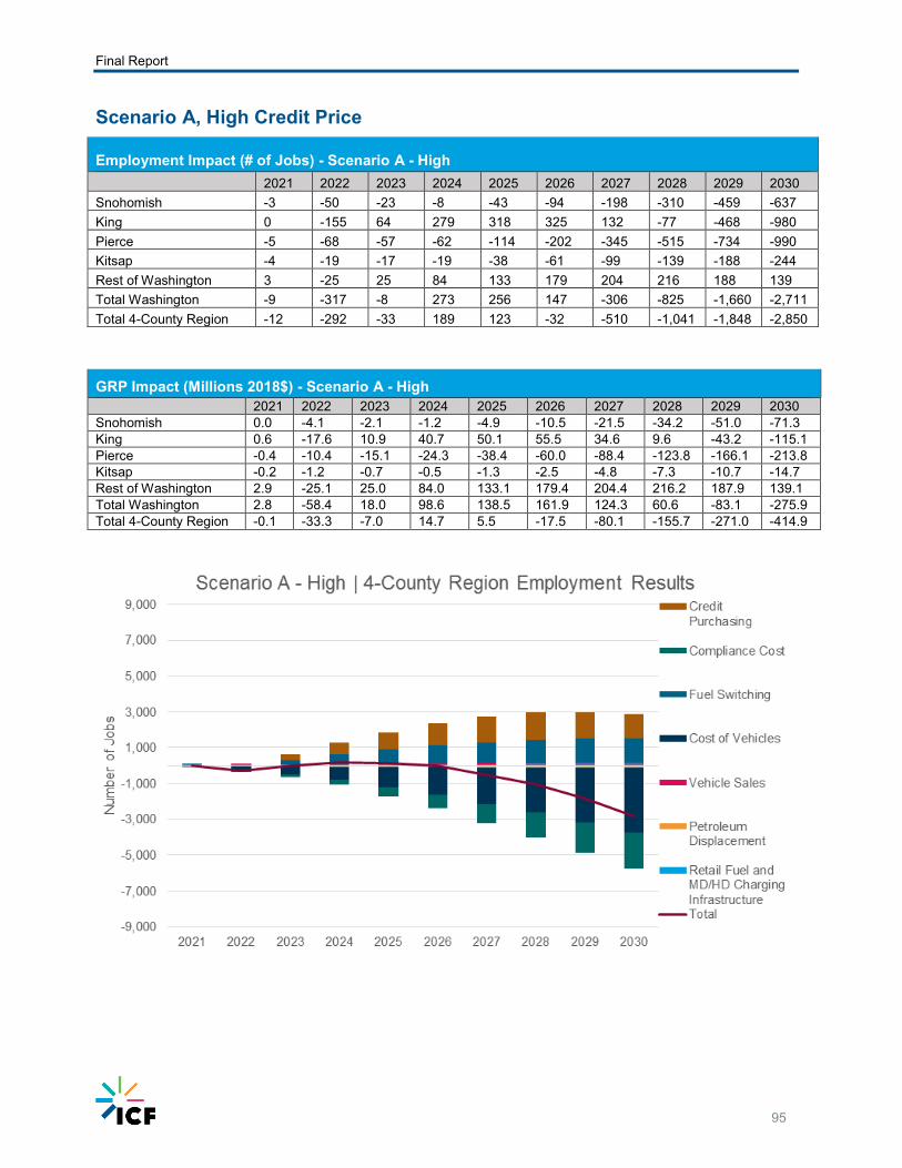
Scenario A, High Credit Price
Employment Impact (# of Jobs) - Scenario A - High 2021 2022 2023 2024 2025 2026 2027 2028 2029 2030 Snohomish -3 -50 -23 -8 -43 -94 -198 -310 -459 -637 King 0 -155 64 279 318 325 132 -77 -468 -980 Pierce -5 -68 -57 -62 -114 -202 -345 -515 -734 -990 Kitsap -4 -19 -17 -19 -38 -61 -99 -139 -188 -244 Rest of Washington 3 -25 25 84 133 179 204 216 188 139 Total Washington -9 -317 -8 273 256 147 -306 -825 -1,660 -2,711 Total 4-County Region -12 -292 -33 189 123 -32 -510 -1,041 -1,848 -2,850
GRP Impact (Millions 2018$) - Scenario A - High
2021 2022 2023 2024 2025 2026 2027 2028 2029 2030 Snohomish 0.0 -4.1 -2.1 -1.2 -4.9 -10.5 -21.5 -34.2 -51.0 -71.3 King 0.6 -17.6 10.9 40.7 50.1 55.5 34.6 9.6 -43.2 -115.1 Pierce -0.4 -10.4 -15.1 -24.3 -38.4 -60.0 -88.4 -123.8 -166.1 -213.8 Kitsap -0.2 -1.2 -0.7 -0.5 -1.3 -2.5 -4.8 -7.3 -10.7 -14.7 Rest of Washington 2.9 -25.1 25.0 84.0 133.1 179.4 204.4 216.2 187.9 139.1 Total Washington 2.8 -58.4 18.0 98.6 138.5 161.9 124.3 60.6 -83.1 -275.9 Total 4-County Region -0.1 -33.3 -7.0 14.7 5.5 -17.5 -80.1 -155.7 -271.0 -414.9

Final Report
96
Scenario B: Aggressive Electrification
Scenario B, Low Credit Price
Employment Impact (# of Jobs) - Scenario B - Low 2021 2022 2023 2024 2025 2026 2027 2028 2029 2030 Snohomish 21 8 59 95 80 28 -51 -141 -237 -352 King 85 45 311 547 585 485 294 70 -175 -492 Pierce 26 7 39 46 3 -90 -212 -362 -520 -698 Kitsap 6 1 12 17 6 -15 -44 -77 -111 -150 Rest of Washington 14 7 62 115 145 154 154 142 122 93 Total Washington 151 68 483 820 820 562 140 -368 -921 -1,600 Total 4-County Region 138 61 421 704 675 408 -14 -510 -1,043 -1,693
GRP Impact (Millions 2018$) - Scenario B - Low
2021 2022 2023 2024 2025 2026 2027 2028 2029 2030 Snohomish 1.7 0.7 4.9 7.7 5.9 0.2 -8.4 -18.8 -30.3 -44.0 King 9.0 5.3 40.4 73.0 81.5 70.9 47.0 15.6 -21.0 -69.7 Pierce 2.4 -1.4 -3.4 -11.6 -25.3 -46.3 -72.0 -104.6 -139.8 -177.8 Kitsap 0.4 0.2 1.1 1.8 1.4 0.2 -1.6 -3.7 -6.0 -8.9 Rest of Washington 13.8 6.8 61.6 115.4 145.4 153.6 154.3 141.8 121.9 92.5 Total Washington 27.4 11.6 104.7 186.3 208.9 178.7 119.4 30.3 -75.2 -207.9 Total 4-County Region 13.6 4.8 43.1 70.9 63.5 25.1 -34.9 -111.4 -197.1 -300.4
Final Report
97
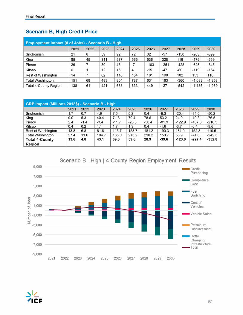
Scenario B, High Credit Price
Employment Impact (# of Jobs) - Scenario B - High 2021 2022 2023 2024 2025 2026 2027 2028 2029 2030 Snohomish 21 8 59 92 72 32 -57 -150 -263 -399 King 85 45 311 537 565 536 328 116 -179 -559 Pierce 26 7 39 43 -7 -103 -251 -428 -625 -848 Kitsap 6 1 12 16 4 -15 -47 -80 -119 -164 Rest of Washington 14 7 62 116 154 181 190 182 153 110 Total Washington 151 68 483 804 787 631 163 -360 -1,033 -1,858 Total 4-County Region 138 61 421 688 633 449 -27 -542 -1,185 -1,969
GRP Impact (Millions 2018$) - Scenario B - High
2021 2022 2023 2024 2025 2026 2027 2028 2029 2030 Snohomish 1.7 0.7 4.9 7.5 5.2 0.4 -9.3 -20.4 -34.0 -50.2 King 9.0 5.3 40.4 71.8 79.4 78.6 53.2 24.0 -19.3 -76.5 Pierce 2.4 -1.4 -3.4 -11.7 -26.3 -50.4 -81.9 -122.9 -167.8 -216.5 Kitsap 0.4 0.2 1.1 1.7 1.3 0.4 -1.6 -3.7 -6.4 -9.6 Rest of Washington 13.8 6.8 61.6 115.7 153.7 181.2 190.3 181.9 152.8 110.5 Total Washington 27.4 11.6 104.7 185.0 213.2 210.2 150.7 58.9 -74.6 -242.3 Total 4-County Region
13.6 4.8 43.1 69.3 59.6 28.9 -39.6 -123.0 -227.4 -352.8
Final Report
98
Scenario C: Mixed Technology Scenario
Scenario C, Low Credit Price
Employment Impact (# of Jobs) - Scenario C - Low 2021 2022 2023 2024 2025 2026 2027 2028 2029 2030 Snohomish -28 -51 -4 58 72 53 7 -58 -134 -239
King -97 -180 112 513 712 762 719 581 379 58
Pierce -36 -91 -73 -48 -64 -133 -223 -357 -509 -690
Kitsap -11 -20 -10 2 1 -9 -27 -49 -74 -107
Rest of Washington -13 -44 12 90 144 168 187 174 135 74
Total Washington -185 -386 36 616 865 841 664 291 -203 -905
Total 4-County Region -172 -342 25 526 720 673 477 117 -338 -979
GRP Impact (Millions 2018$) - Scenario C - Low
2021 2022 2023 2024 2025 2026 2027 2028 2029 2030 Snohomish -2.1 -4.1 -0.2 5.1 6.1 3.9 -1.2 -8.9 -18.3 -30.9 King -10.0 -19.7 19.3 74.8 107.4 120.5 121.6 107.0 80.2 34.1 Pierce -3.4 -16.9 -23.7 -33.7 -47.8 -70.2 -94.1 -127.9 -166.0 -207.9 Kitsap -0.7 -1.3 -0.4 0.8 1.0 0.6 -0.3 -1.7 -3.5 -5.9 Rest of Washington -12.8 -43.9 11.7 89.6 144.2 167.7 187.4 173.7 134.7 73.9 Total Washington -28.9 -85.9 6.6 136.6 210.9 222.5 213.3 142.1 27.2 -136.8 Total 4-County Region -16.2 -42.0 -5.0 47.0 66.7 54.8 25.9 -31.6 -107.5 -210.6
Final Report
99
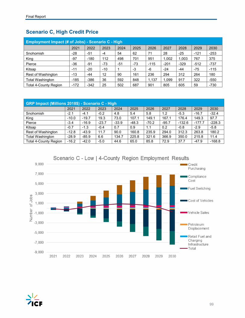
Scenario C, High Credit Price
Employment Impact (# of Jobs) - Scenario C - High 2021 2022 2023 2024 2025 2026 2027 2028 2029 2030 Snohomish -28 -51 -4 54 62 71 28 -25 -121 -253 King -97 -180 112 498 701 951 1,002 1,003 767 375 Pierce -36 -91 -73 -51 -73 -115 -201 -329 -512 -737 Kitsap -11 -20 -10 1 -3 -6 -24 -44 -75 -115 Rest of Washington -13 -44 12 90 161 236 294 312 264 180 Total Washington -185 -386 36 592 848 1,137 1,099 917 322 -550 Total 4-County Region -172 -342 25 502 687 901 805 605 59 -730
GRP Impact (Millions 2018$) - Scenario C - High
2021 2022 2023 2024 2025 2026 2027 2028 2029 2030 Snohomish -2.1 -4.1 -0.2 4.8 5.4 5.8 1.2 -5.3 -16.7 -32.4 King -10.0 -19.7 19.3 73.0 107.1 149.1 167.1 176.4 149.3 97.7 Pierce -3.4 -16.9 -23.7 -33.9 -48.3 -70.2 -95.7 -132.6 -177.7 -228.3 Kitsap -0.7 -1.3 -0.4 0.7 0.9 1.1 0.2 -0.8 -2.9 -5.8 Rest of Washington -12.8 -43.9 11.7 90.0 160.8 235.9 294.0 312.3 263.8 180.2 Total Washington -28.9 -85.9 6.6 134.7 225.8 321.6 366.9 350.0 215.8 11.4 Total 4-County Region -16.2 -42.0 -5.0 44.6 65.0 85.8 72.9 37.7 -47.9 -168.8

Final Report
100
Scenario D: All-In, Maximum Feasible Reduction
Scenario D, Low Credit Price
Employment Impact (# of Jobs) - Scenario D - Low 2021 2022 2023 2024 2025 2026 2027 2028 2029 2030 Snohomish -16 -51 -38 10 58 83 113 149 187 173 King -79 -263 -174 101 346 478 628 801 957 905 Pierce -34 -133 -241 -353 -443 -524 -574 -590 -596 -651 Kitsap -7 -17 -11 4 20 31 44 58 72 68 Rest of Washington -14 -56 -13 34 40 15 -20 -57 -102 -174 Total Washington -151 -520 -478 -204 22 83 191 361 519 321 Total 4-County Region -136 -463 -465 -238 -18 69 211 418 620 495
GRP Impact (Millions 2018$) - Scenario D - Low
-0.8 -3.5 -3.0 -0.1 2.8 3.9 5.4 7.6 10.2 7.4 Snohomish -6.5 -26.1 -11.6 26.2 61.2 82.7 107.1 133.8 156.9 148.1 King -3.3 -26.3 -53.0 -92.6 -133.6 -171.1 -203.6 -229.2 -251.8 -277.9 Pierce -0.5 -1.3 -0.9 0.2 1.5 2.3 3.3 4.4 5.5 5.3 Kitsap -14.4 -56.4 -13.2 33.9 40.2 14.7 -19.7 -56.9 -101.5 -173.9 Rest of Washington -25.6 -113.5 -81.8 -32.4 -28.0 -67.5 -107.5 -140.2 -180.8 -291.0 Total Washington -11.2 -57.2 -68.6 -66.3 -68.1 -82.3 -87.8 -83.4 -79.2 -117.1 Total 4-County Region -0.8 -3.5 -3.0 -0.1 2.8 3.9 5.4 7.6 10.2 7.4
Final Report
101
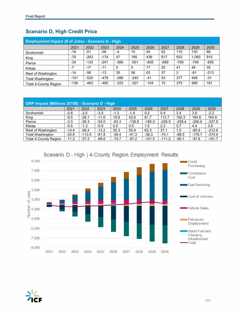
Scenario D, High Credit Price
Employment Impact (# of Jobs) - Scenario D - High 2021 2022 2023 2024 2025 2026 2027 2028 2029 2030 Snohomish -16 -51 -38 -4 10 45 62 110 130 86
King -79 -263 -174 47 185 439 617 933 1,060 915
Pierce -34 -133 -241 -366 -501 -605 -689 -709 -748 -855
Kitsap -7 -17 -11 0 5 17 25 41 48 35
Rest of Washington -14 -56 -13 35 56 63 37 2 -81 -213
Total Washington -151 -520 -478 -288 -245 -41 53 377 408 -31
Total 4-County Region -136 -463 -465 -323 -301 -104 15 375 489 181
GRP Impact (Millions 2018$) - Scenario D - High 2021 2022 2023 2024 2025 2026 2027 2028 2029 2030 Snohomish -0.8 -3.5 -3.0 -1.3 -1.4 0.2 0.4 3.4 3.9 -2.3 King -6.5 -26.1 -11.6 19.9 42.6 81.7 112.7 162.3 184.6 164.9 Pierce -3.3 -26.3 -53.0 -93.3 -138.8 -185.0 -226.5 -259.4 -290.6 -327.9 Kitsap -0.5 -1.3 -0.9 0.0 0.5 1.5 2.3 3.7 4.4 3.6 Rest of Washington -14.4 -56.4 -13.2 35.3 55.9 63.3 37.1 1.5 -80.9 -212.6 Total Washington -25.6 -113.5 -81.8 -39.4 -41.3 -38.3 -74.1 -88.5 -178.7 -374.4 Total 4-County Region -11.2 -57.2 -68.6 -74.7 -97.2 -101.5 -111.2 -90.1 -97.8 -161.7
Final Report
102
Appendix C: Supplemental Data Available The following data and files have been supplied to PSCAA to support this project:
- WA-GREET
- C-LINE run output and receptor concentrations
- Population and BenMAP results
- AQ Data layers
Final Report
103
Appendix D: Erratum November 7, 2019
Subsequent to the release of the final report:
ICF discovered that there was an error in the code that was used to develop the compliance scenario model used in the analysis as part of the work for the Puget Sound Clean Air Agency. The error was linked to the increased use of natural gas (primarily renewable) as a transportation fuel in heavy-duty trucks (Class 7-8). In short, as natural gas consumption increased, the model included a displacement of conventional diesel at a rate that was inconsistent with (greater than) what should be considered. This error manifested itself when natural gas as a transportation fuel consumption was modeled to increase over baseline usage—which was most significant in Scenario D, with small increases in Scenario C. There was no increase in the use of natural gas above baseline in Scenario A nor Scenario B. For Scenario C and D, this error led to less-than-anticipated diesel consumption. After fixing this error, ICF identified the following high-level impacts on our results, with a focus on the compliance curve and potential economic impacts.
• There is no discernable impact on ICF’s modeled compliance. After correcting for the error regarding diesel consumption, there were an increased number of deficits calculated. However, both biodiesel and renewable diesel are calculated as a percent blend in the model (as opposed to a fixed volume to prevent blending at a rate too high over time). In other words, as the diesel volumes were corrected, increased volumes of biodiesel and renewable diesel effectively offset the deficit generation with credit generation.
• ICF estimates no discernable impact on the economic modeling results. As noted throughout the report, the economic modeling results are small across all scenarios. There are several reasons for our estimates that there are no impacts on the modeling results.
o Small change in the compliance cost pass-through (compliance cost). ICF models the compliance cost to consumers as a full pass-through of the compliance cost associated with illustrative credit price curves used in the analysis. This pass-through cost is modeled as the cost of all deficits. The compliance cost is calculated as the product of the sum of all deficits generated in a given year and the credit price in that year. After correcting for the error, more deficits were generated, but the impact is spread over a larger volume of fuel. On a net basis, the compliance cost pass-through assumption increases, but the per gallon change is unaffected. Impact: small negative economic impacts.
o Small change to refinery impacts (petroleum displacement). As noted in the report, ICF accounts for displaced diesel (and gasoline) as a net negative impact to the refining industry—by displacing half the product and assuming the other half is shipped out of the region at a higher cost. Our modeling over-stated diesel displacement and as a result over-states the impacts on the refining industry. Impact: small positive economic impacts.
o Small change to biofuel impacts (credit purchasing). Both renewable diesel and biodiesel are linked as a percentage blend to total diesel consumption in our modeling. As a result, when the diesel volumes were too low, the amount of renewable diesel and biodiesel blended was also too low. When correcting the
Final Report
104
error, both volumes increased, as did credit generating activity for both fuels. ICF links the value generated by those credits back to the corresponding low carbon fuel industry, so there would be increased flow of that revenue in the corrected model. Impact: small positive economic impacts.
o No other change. There are no other anticipated changes in the economic modeling results, as the corrected change has no impact on vehicle sales or cost of vehicles, infrastructure investments, or fuel switching.
Summary. The identified error has no impact on ICF conclusions regarding the carbon intensity reduction of 26% achieved in Scenario D. Further, ICF estimates that there will be no discernible change to economic modeling results as a result of fixing the identified error in the scenario modeling analysis because the two small positive impacts outlined above are expected to offset the small negative impact.
The error also has no impact on the air quality analysis because that analysis was derived from the projected vehicle fleet composition, activity, and emission factors, not the total fuel volumes.
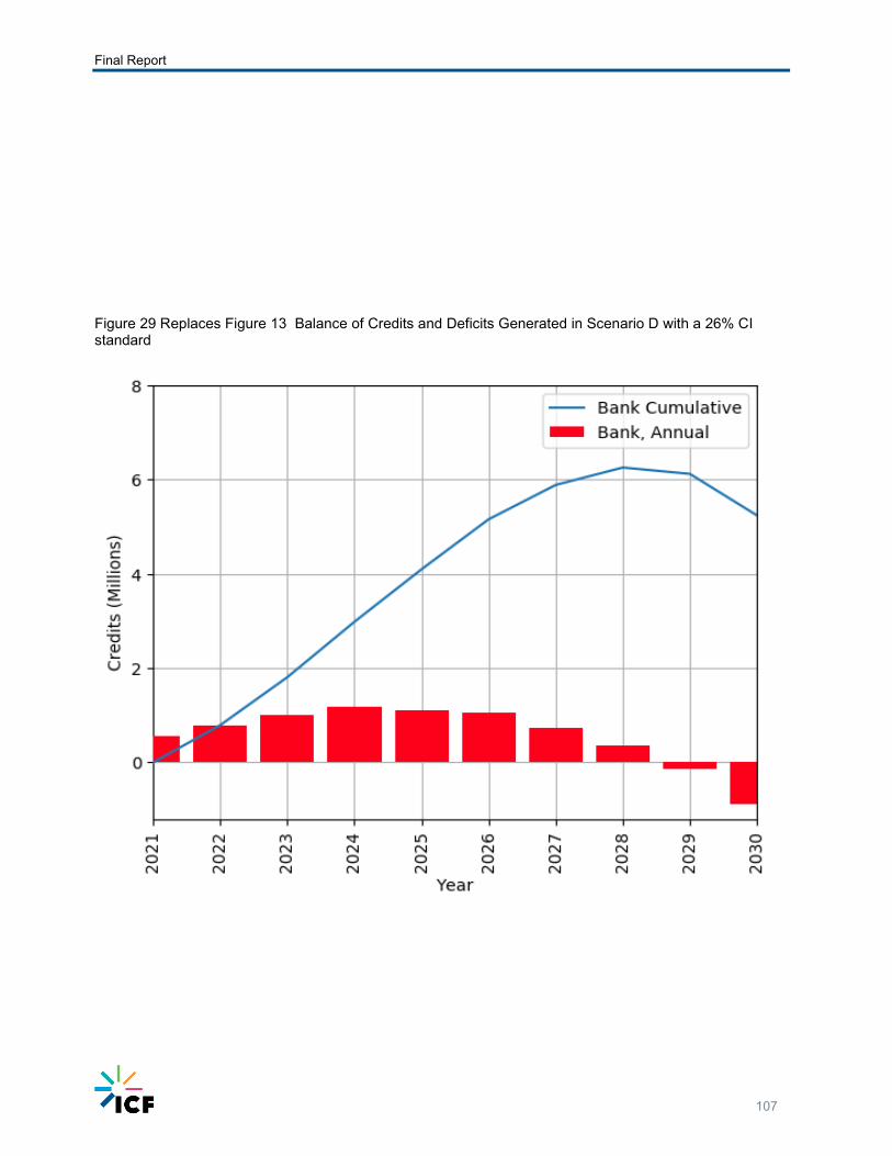
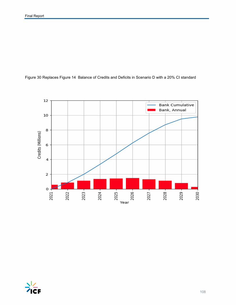
The following, corrected figures replace Figures 11-15 (on pages 38-42). For a quantitative comparison, the corrected (and old) Cumulative Credit Bank values in 2030 are:
• for Scenario C, 5.22 (4.93) million credits • for Scenario D (with a 26% CI reduction target), 5.24 (4.89) million credits • for Scenario D (with a 20% CI reduction target), 9.76 (9.01) million credits
Final Report
105
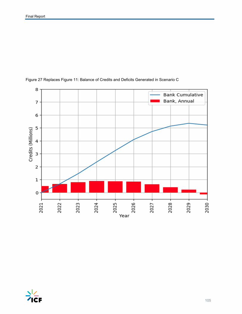
Figure 27 Replaces Figure 11: Balance of Credits and Deficits Generated in Scenario C
Final Report
106
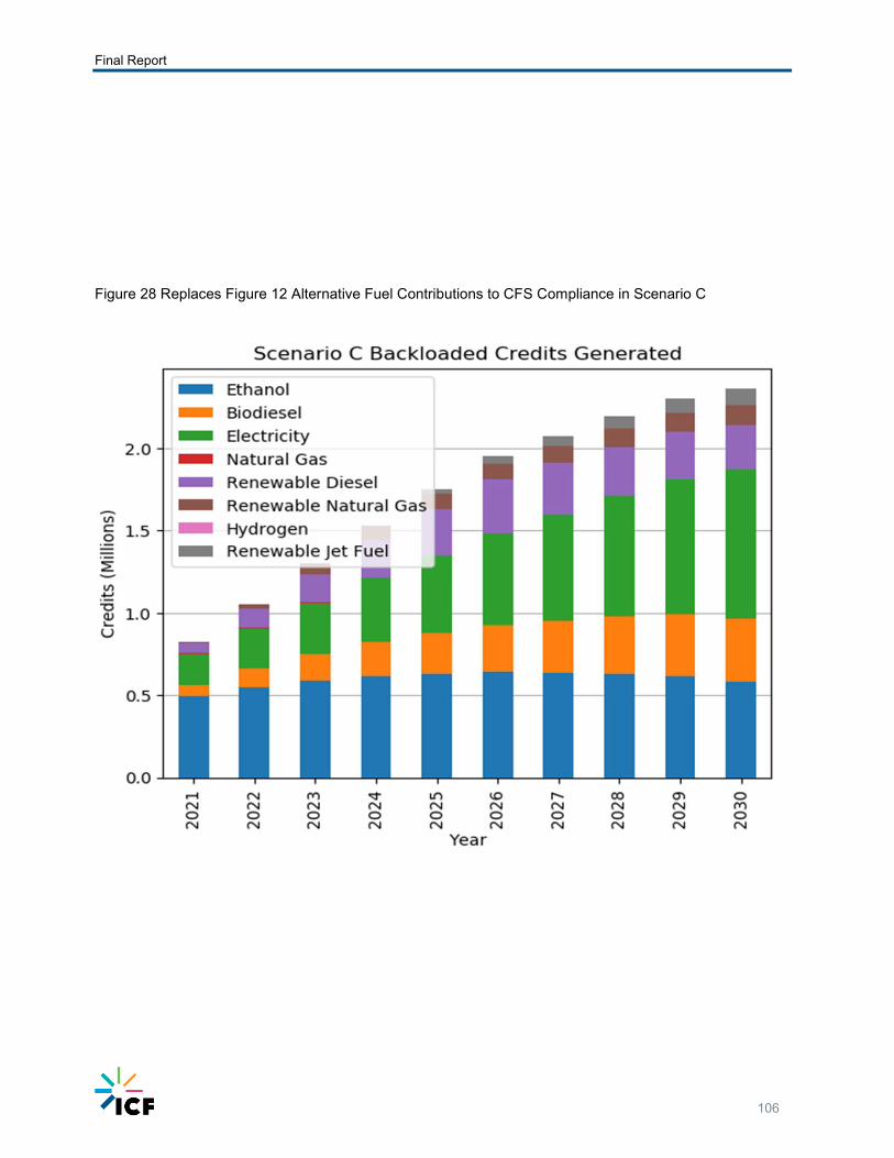
Figure 28 Replaces Figure 12 Alternative Fuel Contributions to CFS Compliance in Scenario C
Final Report
107
Figure 29 Replaces Figure 13 Balance of Credits and Deficits Generated in Scenario D with a 26% CI standard
Final Report
108
Figure 30 Replaces Figure 14 Balance of Credits and Deficits in Scenario D with a 20% CI standard

Final Report
109
Figure 31 Replaces Figure 15 Alternative Fuel Contributions to CFS Compliance in Scenario D with a 26% CI standard
Related Documents