Appendix 8B Sacramento River Ecological Flows Line items and numbers identified or noted as “No Action Alternative” represent the “Existing Conditions/No Project/No Action Condition” (described in Chapter 2 Alternatives Analysis). Table numbering may not be consecutive for all appendixes.

Welcome message from author
This document is posted to help you gain knowledge. Please leave a comment to let me know what you think about it! Share it to your friends and learn new things together.
Transcript

Appendix 8B Sacramento River Ecological Flows
Line items and numbers identified or noted as “No Action Alternative” represent the “Existing Conditions/No Project/No Action Condition” (described in Chapter 2 Alternatives Analysis). Table numbering may not be consecutive for all appendixes.

This page intentionally left blank.

NODOS AnalysisCorrected Literature Cited

This page intentionally left blank.

Analysis of the North-of-the-Delta
Offstream Storage Investigation
Prepared for
Statewide Infrastructure Investigations Branch
Prepared by
Sacramento River Project
500 Main St.
Chico, CA 95928
and
600 - 2695 Granville St.
Vancouver, BC
Canada V6H 3H4
October 4, 2012

Citation: The Nature Conservancy and ESSA Technologies Ltd. 2012. SacEFT Analysis of the North-of-the-Delta
Offstream Storage Investigation. The Nature Conservancy, Chico, CA. 73pp + appendices.
Any inquiries regarding this report should be directed to:
Ryan Luster
Project Director
Sacramento River Project
The Nature Conservancy
190 Cohasset Road, Suite 177
Chico, CA 95926
(530) 809-2663
© 2012 The Nature Conservancy
No part of this publication may be reproduced, stored in a retrieval system, or transmitted, in any form or by any
means, electronic, mechanical, photocopying, recording, or otherwise, without prior written permission from The
Nature Conservancy.

SacEFT Effects Analysis: NODOS
i
Table of Contents
List of Tables ................................................................................................................................................................ ii
List of Figures ............................................................................................................................................................. iv
1. Introduction .......................................................................................................................................................... 1
1.1 Complementary Modeling Paradigms ...................................................................................................... 2
1.1.1 Classes of eFlow Assessment Tools ..................................................................................... 3
1.2 North-of-the-Delta Offstream Storage Investigation ................................................................................ 5
1.2.1 Ecosystem Enhancement Actions ......................................................................................... 6
2. Methodology and Assumptions ........................................................................................................................... 8
2.1 SacEFT’s Focal Species and Performance Measures ............................................................................... 8
2.1.1 Aquatic Species and Performance Measures ........................................................................ 9
2.1.2 Riparian Species and Performance Measures ..................................................................... 11
2.2 Ecological Flows Tool – Core Concepts ................................................................................................ 12
2.3 Locations of Interest and Life-History Timing Assumptions ................................................................. 16
2.4 Special Conditions and Limitations ....................................................................................................... 22
2.5 Focal Comparisons ................................................................................................................................. 22
2.5.1 SacEFT Gravel Augmentation and Bank Protection Alternatives ...................................... 22
3. Results and Discussion ....................................................................................................................................... 28
3.1 Study Flows and Water Temperatures ................................................................................................... 28
3.2 Performance of Alternatives: Overall Synthesis .................................................................................... 33
3.3 Aquatic Species and Performance Measures .......................................................................................... 40
3.3.1 Green Sturgeon ................................................................................................................... 40
3.3.2 Steelhead Trout ................................................................................................................... 43
3.3.3 Fall Chinook ....................................................................................................................... 53
3.3.4 Late Fall Chinook ............................................................................................................... 53
3.3.5 Spring Chinook ................................................................................................................... 53
3.3.6 Winter Chinook .................................................................................................................. 53
3.4 Riparian Species and Performance measures ......................................................................................... 54
3.4.1 Fremont Cottonwood Initiation .......................................................................................... 54
3.4.2 Bank Swallow Habitat Potential and Nest Inundation ........................................................ 60
3.4.3 Large Woody Debris Recruitment ...................................................................................... 62
3.5 Integrated SacEFT Target and Avoidance Flows ................................................................................... 64
4. Conclusions ......................................................................................................................................................... 67
5. Literature Cited .................................................................................................................................................. 68
6. Further Reading ................................................................................................................................................. 70
6. Appendix A – Inverse Correlation between Juvenile Stranding and Juvenile Rearing in SacEFT ............ 74
Appendix B – Indicator Thresholds and Rating System ........................................................................................ 79
Appendix C – Additional Chinook Reports............................................................................................................. 86
C.1 Steelhead ................................................................................................................................................ 86
C.2 Fall Chinook ........................................................................................................................................... 93
C.3 Late Fall Chinook ................................................................................................................................. 100
C.4 Spring Chinook .................................................................................................................................... 107
C.5 Winter Chinook .................................................................................................................................... 114

SacEFT Effects Analysis: NODOS
ii
List of Tables
Table 1-A: Interim Plan Formulation Alternatives – NODOS Investigation. Details subject to change.
Information provided by the NODOS investigation planning team, DWR (August 2011). ..................... 6
Table 2-A: SacEFT focal species, ecological objectives, and performance measures. .............................................. 9
Table 2-B: Spatial location and extent of physical datasets, linked models and performance measures for
the non-salmonid focal species. Performance measures (PMs) for the species are summarized in
Table 2-A. Vertical bars denote PMs that are simulated for river segments; dots denote those
that are simulated (measured in the case of gauges) at points along the river. Q = river
discharge. T = water temperature. Annotation details are listed in Table 2-D. ...................................... 18
Table 2-C: Spatial location and extent of physical datasets, linked models and performance measures for
the salmonid focal species. Performance measures (PMs) for the species are summarized in
Table 2-A. Vertical bars denote PMs that are simulated for river segments; dots denote those
that are simulated (measured in the case of gauges) at points along the river. Q = river
discharge. T = water temperature. Annotation details are listed in Table 2-D. ...................................... 19
Table 2-D: Annotations for Table 2-B and Table 2-C. ............................................................................................. 20
Table 2-E: Summary of the life-history timing information relevant to the SacEFT focal species. Only those
performance measures requiring information on life history timing are included here.
Abbreviations of performance measures (PMs) are described in Table 2-A. Time intervals
marked with heavy color denote periods of greater importance to focal species. In the case of
the spawning PMs (CS-1), heavily shaded regions denote for each salmonid run-type/species the
period between the 25th and 75
th percentile, when half the spawning takes place. In the case of
the other salmonid PMs, the heavily shaded regions denote the period between the 25th and 75
th
percentile of the population are present. Specific timing of CS-2, 3, 4, 5, 6 depends on ambient
water temperature and varies with discharge scenario and year. Juvenile residency is defined by
a fixed 90 day period following emergence for Chinook and a 365 day period for steelhead. This
table is based on SALMOD (Bartholow and Heasley 2006, ultimately Vogel and Marine 1991).
Salmonid timing values shown here are typical and may shift by as much as five days earlier or
later, depending on year and reach. Timing values for green sturgeon, cottonwood and bank
swallow are based on workshop discussions, and all values are under user control. ............................. 21
Table 2-F: Potential revetment removal sites on the middle Sacramento River. Sites 2-6 define the “rip rap
removal” scenario in SacEFT. For details see Larsen (2007). ............................................................... 24
Table 3-A: Rank order of preferred NODOS alternative by focal species or group based on synthesis results
in Table 3-B. .......................................................................................................................................... 33
Table 3-B: High-level summary of the relative direction of change in performance measures between
existing conditions and the different alternatives. Numbers in brackets refer to the increased
percentage of simulation years having a favorable rating. **Results of these meander/erosion
model dependent performance measures are for the Sacramento River channel with existing
revetment (no revetment removal). ........................................................................................................ 34
Table 3-C: High-level summary of the relative direction of change in performance measures between the
No Action Alternative and the different alternatives. Numbers in brackets refer to the increased
percentage of simulation years having a favorable rating. **Results of these meander/erosion
model dependent performance measures are for the Sacramento River channel with existing
revetment (no revetment removal). ........................................................................................................ 36
Table 3-D: High-level summary of the relative direction of change in performance measures between the
No Action Alternative (which reflects 2030 conditions, constraints and operations) and
historical flows. Numbers in brackets refer to the increased percentage of simulation years
having a favorable rating. **Results of these meander/erosion model dependent performance
measures are for the Sacramento River channel with existing revetment (no revetment removal). ....... 38

SacEFT Effects Analysis: NODOS
iii

SacEFT Effects Analysis: NODOS
iv
List of Figures
Figure 1.1: Attributes of alternative ecological flow assessment tools showing placement of the Sacramento
River Ecological Flows Tool (SacEFT; ESSA (2011)). IHA = Indicators of Hydrologic
Alteration (Mathews and Richter 2007). HAT = Hydrologic Assessment Tool (Kennen et al.
2009). RVA = Range of Variability Analysis (Mathews and Richter 2007). HEC-EFM =
Hydrologic Engineering Center Ecosystem Functions Model (USACE 2002). IOS = Winter-run
Chinook IOS/DPM. SALMOD = Salmonid Population Model (Bartholow et al. 2002). ........................ 4
Figure 1.2: Artist’s rendition of Sites Reservoir (a) and its location relative to the Sacramento River (b).
Note: bottom panel (b) is for illustration purposes only, and is not intended to represent the final
or preferred Plan Alternative. NODOS alternatives all include three conveyance facilities: TC
Canal, GCID Canal and Delevan pipeline. ............................................................................................... 5
Figure 2.1: Typical SacEFT output showing annual roll-up results for the Fremont cottonwood initiation
(FC1) performance measure. Analogous plots are available for all of the tools’ focal species and
performance measures. ........................................................................................................................... 13
Figure 2.2: Annual roll-up results for the SacEFT Fremont cottonwood initiation (FC1) performance
measure run using historic observed flows (WY1938–2003). This calibration also takes into
consideration comparisons with aerial photographs of historically strong Cottonwood
recruitment at study sites vs. model results. ........................................................................................... 13
Figure 2.3: Typical SacEFT output showing multi-year roll-up results for the Fremont cottonwood initiation
(FC1) performance measure. Analogous plots are available for all of the tools’ focal species and
performance measures. ........................................................................................................................... 15
Figure 2.4: Example SacEFT output report showing results for the Fremont cottonwood initiation (FC1)
performance measure at a specific cross-section at the conclusion of the seed dispersal period in
WY1997. ................................................................................................................................................ 15
Figure 2.5: Map of the Sacramento River watershed and study area over which the SacEFT will be applied,
from Keswick Dam (RM 301) to Colusa (RM 143) (CALFED Bay-Delta Program 2000). .................. 16
Figure 2.6: Meander Migration/Bank Erosion Model, Woodson Bridge segment showing 2004 revetment
coverage (= SacEFT “no rip rap removal”). ........................................................................................... 25
Figure 2.7: Meander Migration/Bank Erosion Model; Hamilton City segment showing 2004 revetment
coverage (= SacEFT “no rip rap removal”). ........................................................................................... 26
Figure 2.8: Meander Migration/Bank Erosion Model; Ord Ferry segment showing 2004 revetment coverage
(= SacEFT “no rip rap removal”). .......................................................................................................... 27
Figure 3.1: Flow exceedance plots at Keswick, RM301 (Oct-1 to Sep-30) for NODOS alternatives relative
to historical flows. .................................................................................................................................. 28
Figure 3.2: Flow exceedance plots at Bend Bridge near Red Bluff, RM260 (Oct-1 to Sep-30) for NODOS
alternatives relative to historical flows. .................................................................................................. 29
Figure 3.3: Flow exceedance plots near Hamilton City, RM199 (Oct-1 to Sep-30) for NODOS alternatives
relative to historical flows. ..................................................................................................................... 29
Figure 3.4: Flow exceedance plots near Colusa, RM143 (Oct-1 to Sep-30) for NODOS alternatives relative
to historical flows. .................................................................................................................................. 30
Figure 3.5: Water temperature exceedance plots at Keswick, RM301 (Oct-1 to Sep-30) for NODOS
alternatives relative to historical temperatures. ...................................................................................... 31
Figure 3.6: Water temperature exceedance plots at Bend Bridge near Red Bluff, RM260 (Oct-1 to Sep-30)
for NODOS alternatives relative to historical temperatures. .................................................................. 31
Figure 3.7: Water temperature exceedance plots near Hamilton City, RM199 (Oct-1 to Sep-30) for NODOS
alternatives. ............................................................................................................................................ 32

SacEFT Effects Analysis: NODOS
v
Figure 3.8: Water temperature exceedance plots near Colusa, RM143 (Oct-1 to Sep-30) for NODOS
alternatives. ............................................................................................................................................ 32
Figure 3.9: Multi-year roll-up results for green sturgeon thermal egg mortality (GS1). .......................................... 40
Figure 3.10: The percentage of years in each NODOS simulation having favorable (green) conditions for
green sturgeon thermal egg mortality (GS1). Bars labeled with “Change” refer to the % change
between the simulated alternative and the reference condition (either Existing conditions or the
No Action Alternative (NAA)). ............................................................................................................. 40
Figure 3.11: Number of days in each simulation where water temperatures near Hamilton City (RM199) are
greater than 20°C. Bars labeled with “Change” refer to the change in number of days greater than 20°C between the simulated alternative and the reference condition (either Existing conditions or the No Action Alternative (NAA)). .................................................................................. 41
Figure 3.12: Target/favorable water temperature profiles (green) for minimizing green sturgeon thermal egg
mortality (GS1) at two index locations (RM260 and RM199). Water temperature profiles in
green refer to years where SacEFT’s annual performance measure rating was assessed as
good/favorable. The heavy black line provides the median of the all year favorable water
temperature profiles. Lines in red show example years rated as poor by SacEFT (i.e., highest
category of egg mortality). Horizontal lines at 17°C and 20°C are important thresholds that affect green sturgeon egg development (GS1). [Note: this figure is designed for color printing]. ........ 42
Figure 3.13: SacEFT detailed output report for a specific water year (1977) showing daily results for green
sturgeon thermal egg mortality (GS1) at a specific index location (Hamilton City). ............................. 43
Figure 3.14: The percentage of years in each NODOS simulation having favorable (green) conditions for
Steelhead spawning WUA (ST1). Bars labeled with “Change” refer to the % change between
the simulated alternative and the reference condition (either Existing conditions or the No
Action Alternative (NAA)). ................................................................................................................... 44
Figure 3.15: The percentage of years in each NODOS simulation having favorable (green) conditions for
Steelhead redd dewatering (ST6). Bars labeled with “Change” refer to the % change between
the simulated alternative and the reference condition (either Existing conditions or the No
Action Alternative (NAA)). ................................................................................................................... 44
Figure 3.16: The percentage of years in each NODOS simulation having favorable (green) conditions for
Steelhead redd scour (ST5). Bars labeled with “Change” refer to the % change between the
simulated alternative and the reference condition (either Existing conditions or the No Action
Alternative (NAA)). ............................................................................................................................... 45
Figure 3.17: The percentage of years in each NODOS simulation having favorable (green) conditions for
Steelhead juvenile stranding (ST4). Bars labeled with “Change” refer to the % change between
the simulated alternative and the reference condition (either Existing conditions or the No
Action Alternative (NAA)). ................................................................................................................... 45
Figure 3.18: The percentage of years in each NODOS simulation having favorable (green) conditions for
Steelhead rearing WUA (ST2). Bars labeled with “Change” refer to the % change between the
simulated alternative and the reference condition (either Existing conditions or the No Action
Alternative (NAA)). ............................................................................................................................... 46
Figure 3.19: Target/favorable flow profiles (green) for steelhead spawning WUA (ST1) at Sacramento River
near Red Bluff (RM260). Flow profiles in green refer to years where SacEFT’s annual
performance measure rating was assessed as good/favorable. The heavy black line provides the
median of the all year favorable flow profiles. The grey horizontal line (panel a) is the average
of the median target flow. Flow traces in red (panel b) are examples of typical years rated poor
by SacEFT (i.e., least cumulative spawning habitat potential). [Note: this figure is designed for
color printing]. ....................................................................................................................................... 47
Figure 3.20: Example target/favorable flow profiles (green) for steelhead redd dewatering (ST6) at
Sacramento River near Red Bluff (RM260) (panel a). Flow profiles in green refer to years
where SacEFT’s annual performance measure rating was assessed as good/favorable. Example
flow traces in red (panel b) are examples of typical years rated poor by SacEFT (i.e., highest
values of redd dewatering). .................................................................................................................... 48

SacEFT Effects Analysis: NODOS
vi
Figure 3.21: Target/favorable flow profiles (green) for minimizing steelhead egg scour mortality (ST5) at
Sacramento River near Red Bluff (RM260) (panel a). Flow profiles in green refer to years
where SacEFT’s annual performance measure rating was assessed as good/favorable. The heavy
black line (panel a) provides the median of the all year favorable flow profiles. Example flow
traces in red (panel b) are examples of typical years rated poor by SacEFT (i.e., highest values
of redd scour). Horizontal lines at 55,000 cfs and 75,000 cfs are important thresholds that affect
steelhead egg scour mortality rates (ST5). ............................................................................................. 50
Figure 3.22: Target/favorable flow profiles (green) for minimizing juvenile steelhead stranding mortality
(ST4) at Sacramento River near Red Bluff (RM260) (panel a). Flow profiles in green refer to
years where SacEFT’s annual performance measure rating was assessed as good/favorable. The
heavy black line (panel a) provides the median of the all year favorable flow profiles. Example
flow traces in red (panel b) are examples of typical years rated poor by SacEFT (i.e., highest
values of juvenile stranding). [Note: this figure is designed for color printing]..................................... 51
Figure 3.23: Target/favorable flow profiles (green) for maximizing juvenile steelhead rearing WUA (ST2) at
Sacramento River near Red Bluff (RM260) (panel a). Flow profiles in green refer to years
where SacEFT’s annual performance measure rating was assessed as good/favorable. The heavy
black line (panel a) provides the median of the all year favorable flow profiles. Example flow
traces in red (panel b) are examples of typical years rated poor by SacEFT (i.e., poorest values
for juvenile rearing WUA). [Note: this figure is designed for color printing]. ...................................... 52
Figure 3.24: Multi-year roll-up results for Fremont cottonwood seedling initiation success (FC1). .......................... 54
Figure 3.25: The percentage of years in each NODOS simulation having favorable (green) conditions for
Fremont cottonwood seedling initiation (FC1). Bars labeled with “Change” refer to the %
change between the simulated alternative and the reference condition (either Existing conditions
or the No Action Alternative (NAA)). ................................................................................................... 54
Figure 3.26: The percentage of years in each NODOS simulation having favorable (green) conditions for
Fremont cottonwood seedling scour (FC2). Bars labeled with “Change” refer to the % change
between the simulated alternative and the reference condition (either Existing conditions or the
No Action Alternative (NAA)). Note: The FC2 performance measure in SacEFT is only
relevant/calculated in years with successful Fremont cottonwood initiation (FC1). .............................. 55
Figure 3.27: Annual index of total number of SacEFT cross-section nodes (entire study area) with
successfully initiating Fremont cottonwood seedlings (FC1). These annual results are sorted in
descending order. Panel (a) shows results for historical flows from 1938 to 2004. Green shaded
bars refer to initiation totals that if met or exceeded, receive a favorable (green) rating in
SacEFT. Panel (b) is for the NODOS existing conditions alternative. Panel (c) gives results for
NODOS Investigation alternative A. Panel (d) shows results for NODOS Investigation
alternative B. Finally, panel (e) shows results for NODOS Investigation alternative C. ....................... 56
Figure 3.28: Target/favorable flow profiles (green) needed to deliver downstream successful Fremont
cottonwood initiation (FC1) as measured at Sacramento River near Red Bluff (RM260). Flow
profiles in green refer to years where SacEFT’s annual performance measure rating was
assessed as good/favorable. [Note: this figure is designed for color printing]. ...................................... 57
Figure 3.29: Target/favorable flow profiles (green) for successful Fremont cottonwood initiation (FC1) at
Sacramento River near Hamilton City (RM199). Flow profiles in green refer to years where
SacEFT’s annual performance measure rating was assessed as good/favorable. [Note: this figure
is designed for color printing]. ............................................................................................................... 58
Figure 3.30: Target/favorable flow profiles (green) for successful Fremont cottonwood initiation (FC1) at
Sacramento River near Butte City (RM168). Flow profiles in green refer to years where
SacEFT’s annual performance measure rating was assessed as good/favorable. [Note: this figure
is designed for color printing]. ............................................................................................................... 58
Figure 3.31: Avoidance flow profiles (red) for failed Fremont cottonwood initiation (FC1) at Sacramento
River near Butte City (RM168) relative to the target flow and recession rate. [Note: this figure is
designed for color printing]. ................................................................................................................... 59

SacEFT Effects Analysis: NODOS
vii
Figure 3.32: Multi-year roll-up results for Bank swallow habitat potential (BASW1). The top panel shows
results for all NODOS alternatives under existing revetment. The bottom panel shows results
with select rock removal (as defined in section 2.5.1). .......................................................................... 60
Figure 3.33: The percentage of years in each NODOS simulation having favorable (green) conditions for
Bank swallow habitat potential/suitability (BASW1). Panel (a) provides results under existing
revetment. Panel (b) shows results with selected rock removal (as defined in section 2.5.1). Bars
labeled with “Change” refer to the % change between the simulated alternative and the
reference condition (either Existing conditions or the No Action Alternative (NAA)).......................... 61
Figure 3.34: The percentage of years in each NODOS simulation having favorable (green) conditions for
Bank swallow nest inundation (BASW1). Bars labeled with “Change” refer to the % change
between the simulated alternative and the reference condition (either Existing conditions or the
No Action Alternative (NAA)). ............................................................................................................. 62
Figure 3.35: Multi-year roll-up results for Large Wood Debris recruitment (LWD) to the mainstem
Sacramento River. The top panel shows results for all NODOS alternatives under existing
revetment. The bottom panel shows results with select rock removal (as defined in section
2.5.1). ..................................................................................................................................................... 62
Figure 3.36: The percentage of years in each NODOS simulation having favorable (green) conditions for
Large Woody Debris recruitment (LWD) to the mainstem Sacramento River. Panel (a) provides
results under existing revetment. Panel (b) shows results with selected rock removal (as defined
in section 2.5.1). Bars labeled with “Change” refer to the % change between the simulated
alternative and the reference condition (either Existing conditions or the No Action Alternative
(NAA)). .................................................................................................................................................. 63
Figure B.1: Typical SacEFT output showing annual roll-up results for the Fremont cottonwood initiation
(FC1) performance measure. Analogous plots are available for all of the tools’ focal species and
performance measures. ........................................................................................................................... 79
Figure B.2: Annual roll-up results for the SacEFT Fremont cottonwood initiation (FC1) performance
measure run using historic observed flows (1938–2003). This calibration also takes into
consideration comparisons with aerial photographs of historically strong Cottonwood
recruitment at study sites vs. model results. ........................................................................................... 80
Figure B.3: Typical SacEFT output showing multi-year roll-up results for the Fremont cottonwood initiation
(FC1) performance measure. Analogous plots are available for all of the tools’ focal species and
performance measures. ........................................................................................................................... 81

This page intentionally left blank.

SacEFT Effects Analysis: NODOS
1
1. Introduction
Report Purpose
This report is intended to provide technical information to inform the evaluation of the North-of-the-Delta
Offstream Storage (NODOS) Investigation (hereafter, the Investigation). Alternatives will be evaluated in
detail in the NODOS EIS/EIR and Feasibility Report. The intended audience of this report is the set of
resource specialists and decision makers associated with the Investigation that are evaluating the
environmental effects and feasibility of alternatives. More specifically, this report presents detailed
modeling results on how a set of focal species associated with the Sacramento River may be impacted
(negatively and positively) by the Investigation’s alternatives. Consistent with the design intent of the
Sacramento River Ecological Flows Tool (SacEFT), this report will also inform interested stakeholders,
decision makers, and the public of environmental trade-offs associated with the alternatives. Analyses
included in this report are not strictly limited to the Investigation’s alternatives. The Nature Conservancy
has also reported on scenarios that include measures (rip rap removal and gravel augmentation) that are
not included in the NODOS alternatives. These scenario features are intended to be informative and are
not specific features of the Investigation’s alternatives.
SacEFT Background
Between 2004 and 2008 the Sacramento River Ecological Flows Study team developed a decision
analysis tool that incorporates physical models of the Sacramento River with biophysical habitat models
for six Sacramento River species (see: www.dfg.ca.gov/ERP/signature_sacriverecoflows.asp). The
Ecological Flows Study treats flow as the “master” variable regulating the form and function of riverine
habitats. The Study included development of a decision-analysis tool, the “Sacramento River Ecological
Flows Tool” (SacEFT) to evaluate the ecological consequences of management-related changes in flow
regime and channel restoration activities (e.g., gravel augmentation and selected removal of bank
armoring) (ESSA 2011). The SacEFT decision support tool emphasizes the clear communication of trade-
offs for key ecosystem targets associated with alternative conveyance, water operations, and climate
futures in the Sacramento River ecoregion.
In SacEFT, we chose representative performance measures for multiple focal species. SacEFT includes
flow and habitat relationships for six different focal species/habitats (Chinook salmon, steelhead, green
sturgeon, bank swallows, channel erosion/migration (large woody debris and western pond turtle), and
Fremont cottonwood). Standardized visualization interfaces allow cross-walking of ecological
consequences over different water operation and channel management alternatives.
Scientifically, SacEFT takes a bottom-up, process-based approach to the relationship between flow and
related aquatic habitat variables and looks at how these variables are tied to key species life-stages and
ecosystem functions. Our work and the input of many expert contributors develops a more complete
understanding of the flow regime and its relation to natural processes and species’ requirements so as to
identify the critical attributes of the flow regime necessary to maintain ecosystem function. The multi-
species, multi-performance measure paradigm provides a “portfolio” approach for assessing how different
flow and habitat restoration combinations suit the different life stages of desired species. In so doing,
SacEFT transparently relates additional attributes of the flow regime to multiple species’ life-history
needs in an overall effort at careful organization of representative functional flow needs. This provides a
robust scientific framework to focus the definition of ecological flow guidelines and contributes to the
understanding of water operation effects on focal species and their habitats.

SacEFT Effects Analysis: NODOS
2
The performance measures and functional relationships built into SacEFT were vetted through multi-
disciplinary workshops and numerous design document reviews. The recommendations of these technical
design workshops and subsequent peer reviews provide the basis for the performance measures and
models that have been developed. Specific details on SacEFT submodels and performance measures are
beyond the scope of this document. Readers are referred to ESSA (2011) for detailed descriptions of
submodels, performance measures and related rules and assumptions. Collectively, the constituent focal
species “submodels” provide twelve (12) performance measures (Table 2-A). Multi-year roll-ups of
annual performance allow users to quickly zoom in on the much smaller set of performance measures
which differ significantly across management scenarios.
A design principle of SacEFT is to leverage existing systems and data sources such as CALSIM II,
USRWQM, USRDOM, historical gauging station records, Meander Migration Model outputs of bank
erosion, and sediment-grain size specific sediment transport models. By leveraging many of the same
physical planning models used in existing environmental, socioeconomic, and water resources planning
evaluations in California, SacEFT provides an “eco plug-in” for water operation studies based on use of
these physical hydrologic/water balance models.
As shown in this report, model outputs include an annual summary view for each water year and a
multiple year “roll-up” view which summarizes results across all years. Both views incorporate a good-
fair-poor performance measure ranking system shown with green, yellow and red colors. Daily site-
specific data that produce the annual roll-up rankings are recorded in database output tables, and can be
used for further analyses. Additionally, more detailed daily and site-specific data are also available for the
different focal species performance measures through Excel output reports in the form of raw data, tables
and graphs. SacEFT’s output interface and reports for trade-off analyses make it clear how actions
implemented for the benefit of one area or focal species may affect (both positively and negatively)
another area or focal species. For example, we can show how altering Sacramento River flows to meet
export pumping schedules in the Delta affects focal species’ performance measures in the Upper and
Middle Sacramento River.
1.1 Complementary Modeling Paradigms
Many agencies and organizations (e.g., The Nature Conservancy (TNC), Bureau of Reclamation (USBR),
Department of Water Resources (DWR), the US Geological Survey (USGS,) and the US Army Corps of
Engineers (USACE)) have all developed flow modeling tools in response to a need to understand how
flow and riparian land-use changes impact ecosystems. The modeling of ecosystem relationships is often
used to assess ecosystem health or in the case of flow regime assessments, determine trade-offs between
human water uses and ecological needs (Rapport et al. 1998).
Unlike physical modeling, attempting to build detailed ecological models that make accurate predictions
of ecosystem behavior is challenging and usually not possible in complex, open natural systems (Oreskes
et al. 1994). Because of the high uncertainty and incomplete understanding surrounding the complex
interactions of communities of species with their physical environments (e.g., time-lagged compensatory
density-dependent survival mechanisms) modeling tools like SacEFT emphasize a specific set of species
and life-stage linkages with physical habitat variables. The SacEFT approach does not consider detailed
life-cycle modeling of a single species in an effort to predict precise numbers of emigrating smolts or
returning adult spawners. As with the other modeling tools used in the Investigation, the focus of SacEFT
is determining comparative effects on specific performance indicators. The assumption implicit in
SacEFT is that flows and habitat conditions that generate better outcomes for discrete life-stage
performance measures should – all else being equal – enable the species to support higher adult
abundances. SacEFT also embeds a preferential emphasis on freshwater flow management where

SacEFT Effects Analysis: NODOS
3
resource managers have more influence over conditions, than is practical in the case of marine conditions
and processes (which usually exert a strong influence on adult abundance in salmonids).
In the case of fish species it is recognized that due to compensatory dynamics that can drive population
level responses, that more high-quality habitat at a particular (usually freshwater juvenile) life-stage does
not always translate to a higher abundance of adults. For this reason other modeling efforts pursue full
life-cycle population representations that aim to evaluate the space-time abundance of a particular species
(e.g., Winter-Run Chinook Life Cycle Model (WRCLCM), also known as Winter-run Chinook IOS/DPM
Model or SALMOD). By tracking the abundance and survival of salmon through successive life-stages,
cumulative effects on specific run-types of Chinook salmon populations are simulated.
Given the accepted challenges of “validating” ecological models (Oreskes et al. 1994) many modeling
practitioners favor a weight of evidence approach whereby directional trends in model predictions are
compared across alternative (independently developed) models. Where multiple models determine the
same rank-order results and trends, the strength of the evidence, or degree of belief in those evaluations
increases. Hence, the relative trends in evaluations from life-cycle models provide an important and
complementary line of evidence to SacEFT (and vice versa) in the assessment of flow management
effects. For example, target flows identified by SacEFT could be simulated with IOS/DPM to determine
the expected increase (if any) in total outmigrating winter-run Chinook smolts leaving the Sacramento
River.
1.1.1 Classes of eFlow Assessment Tools
The Winter-run Chinook IOS/DPM, SALMOD and SacEFT all represent tools that fall in the
process-based causal linkage category (Figure 1.1). Process-based models simulate linkages between
flow, in-channel and riparian habitat changes through to a specific change in the survival or productivity
of a particular focal species and life-stage (e.g., success index of Fremont cottonwood (Populus fremontii)
seedling initiation, Chinook salmon (Oncorhynchus tshawytscha) redd de-watering risk). In process-based
models mathematical algorithms are used to describe the time-varying amount and relative suitability of
habitat by drawing empirical relationships between species and environmental variables. These bio-
physical relationships can for example be used to produce a habitat suitability index. Such indices can
then be used to rank flow management alternatives or in the case of the Investigation, make comparisons
with a baseline scenario.
A more widespread class of ecological flow assessment tools emphasizes generalized hydrologic indices
and targets (Figure 1.1). These generalized hydrologic models analyze the changes in flow metrics
themselves and leave it up to the user, outside of the tool, to infer the resultant habitat suitability changes
or otherwise interpret how changes in the hydrologic index might potentially influence a particular
species of concern. Both approaches for assessing and/or prescribing ecological flows are based on the
idea that biological responses are adapted to and shaped by a river basin’s natural hydrologic flow regime
(inter- and intra-annual variability of flow levels and sequences of events) of a river (Poff et al. 1997).
Early work in this area led to a definition of a collection of simple statistical metrics to quantify change in
flow regime, typically after flow regulation (Richter et al. 1996). In an effort to assess how much a flow
regime has been altered, indices of a natural (pre-regulation historical) regime can be compared with the
indices of an altered flow regime. Further research proposed the idea that such statistical indices naturally
have a range of variability, which led to the Range of Variability Analysis (RVA) approach, which can be
used to compare different flow regimes. For these generalized hydrologic models – while there is a great
deal of technical judgment required to interpret the biological significance of performance measure
changes – they provide the advantage of offering simple/readily available input data. Thus, these methods
can be more readily applied in other river basins with lower cost.

SacEFT Effects Analysis: NODOS
4
(+)
(-)(-) (+)
Strength of
causally-
reasoned
linkages
with focal
species
No. of focal habitats and species considered
Process-based functional model
Generalized hydrologic index
IOS
SALMOD
EFT
RVA
HEC-EFMFocus is on changes in flow
metrics themselves
Up to user to
infer impacts on
habitat/species
of concern
HAT
Wide array of experts consulted to develop process-based indicators
Easily used by non-experts
Framework to
organize further
scientific
studies & refine
models over
time (adaptive
management )
Easy to apply in
different
watersheds;
Straightforward
to validate
Does not include every important
ecological function!
IHA
Figure 1.1: Attributes of alternative ecological flow assessment tools showing placement of the
Sacramento River Ecological Flows Tool (SacEFT; ESSA (2011)). IHA = Indicators of
Hydrologic Alteration (Mathews and Richter 2007). HAT = Hydrologic Assessment Tool
(Kennen et al. 2009). RVA = Range of Variability Analysis (Mathews and Richter 2007).
HEC-EFM = Hydrologic Engineering Center Ecosystem Functions Model (USACE 2002).
IOS = Winter-run Chinook IOS/DPM. SALMOD = Salmonid Population Model (Bartholow
et al. 2002).

SacEFT Effects Analysis: NODOS
5
1.2 North-of-the-Delta Offstream Storage Investigation
(a)
(b)
Figure 1.2: Artist’s rendition of Sites Reservoir (a) and its location relative to the Sacramento River (b).
Note: bottom panel (b) is for illustration purposes only, and is not intended to represent the
final or preferred Plan Alternative. NODOS alternatives all include three conveyance
facilities: TC Canal, GCID Canal and Delevan pipeline.
The North-of-the-Delta Offstream Storage (NODOS) Investigation is evaluating potential offstream
surface water storage by constructing Sites Reservoir (pictured above) near the Sacramento River,
downstream from Shasta Dam and west of Maxwell. The high-level project objectives are to:

SacEFT Effects Analysis: NODOS
6
� Improve water supply reliability for agricultural, urban, and environmental uses;
� Improve drinking, agricultural and environmental water quality in the Delta;
� Provide flexible hydropower generation to support integration of renewable energy sources; and
� Increase survival of anadromous and endemic fish populations.
The alternatives considered in this document are summarized in an October 1, 2010 memorandum,
“Assumptions for Existing and Future No Action Alternative Conditions CALSIM II and DSM2
Models.” The assumptions for the NODOS Alternatives are summarized in a January 5, 2011 document,
“Definition of Proposed Alternatives for Evaluation in the North-of-the-Delta Offstream Storage
Administrative Draft Environmental Impact Report and Statement.” High level summaries of major
alternatives are provided in Table 1-A.
Table 1-A: Interim Plan Formulation Alternatives – NODOS Investigation. Details subject to change.
Information provided by the NODOS investigation planning team, DWR (August 2011).
Alternative A B C
Storage Capacity Sites Reservoir 1.27 MAF 1.81 MAF 1.81 MAF Conveyance Capacities (to Sites Reservoir)1 Tehama-Colusa Canal 2,100 cfs 2,100 cfs 2,100 cfs Glenn Colusa Irrigation District Canal 1,800 cfs 1,800 cfs 1,800 cfs New Delevan Pipeline2
Diversion Release
2,000 cfs 1,500 cfs
0 cfs 3
1,500 cfs
2,000 cfs 1,500 cfs
Operations Priorities (Primary Planning Objectives) Long Term (all years) EESA4
Power5 EESA4 Power5
EESA4 Power5
Driest Periods (drought years) M&I M&I M&I Average to Wet Periods (non-drought years)
Water Quality Level 4 Refuge
Agricultural
Water Quality Level 4 Refuge
Agricultural
Water Quality Level 4 Refuge
Agricultural Notes: 1. Diversions through the TC Canal, GCID Canal, and Delevan Pipeline are allowed in any month of the year. 2. New Delevan Pipeline can be operated June through March (April and May are reserved for maintenance). 3. A pump station, intake, and fish screens are not included for the Delevan Pipeline for Alternative B. For Alternative B, the
Delevan Pipeline will be operated for releases only from Sites Reservoir to the Sacramento River year round. 4. Ecosystem Enhancement Storage Account (EESA) related operations are a function of specific conditions, and operating
criteria that are defined uniquely for each action. 5. Includes dedicated pump/generation facilities with an additional dedicated after-bay/fore-bay (enlarged Funks Reservoir) used
for managing conveyance of water between Sites Reservoir and river diversion locations. Key: cfs = cubic feet per second CVP = Central Valley Project EESA = ecosystem enhancement storage account MAF = million acre-feet M&I = municipal and industrial SWP = State Water Project TAF = thousand acre-feet
1.2.1 Ecosystem Enhancement Actions
The proposed NODOS alternatives include the following Ecosystem Enhancement Actions (EEAs):
Action 1. Improve the reliability of coldwater pool storage in Shasta Lake to increase the US Bureau of
Reclamation’s operational flexibility to provide suitable water temperatures in the Sacramento River (see
Action 2 below). This action would operationally translate into the increase of Shasta Lake May storage

SacEFT Effects Analysis: NODOS
7
levels, and increased coldwater pool in storage, with particular emphasis on Below Normal, Dry and
Critical water year types.
Action 2. Provide releases from Shasta Dam of appropriate water temperatures, and subsequently from
Keswick Dam, to maintain mean daily water temperatures year-round at levels suitable for all species and
life-stages of anadromous salmonids in the Sacramento River between Keswick Dam and Red Bluff
Diversion Dam, with particular emphasis on the months of highest potential water temperature-related
impacts (i.e., July through November) during Below Normal, Dry and Critical water year types.
Action 3. Increase the availability of coldwater pool storage in Folsom Reservoir, by increasing May
storage and coldwater pool storage, to allow the U.S. Bureau of Reclamation additional operational
flexibility to provide suitable water temperatures in the lower American River. This action would utilize
additional coldwater pool storage by providing releases from Folsom Dam (and subsequently from
Nimbus Dam) to maintain mean daily water temperatures at levels suitable for juvenile steelhead over-
summer rearing and fall-run Chinook salmon spawning in the lower American River from May through
November during all water year types (not explicitly modeled in CALSIM II).
Action 4. Provide supplemental Delta outflow during summer and fall months (i.e., May through
December) to improve X2 (if possible, west of Collinsville, 81 km) and increase estuarine habitat, reduce
entrainment, and improve food availability for anadromous fishes and other estuarine-dependent species
(e.g., delta smelt, longfin smelt, Sacramento splittail, starry flounder, and the shrimp Crangon
franciscorum).
Action 5. Improve the reliability of coldwater pool storage in Lake Oroville to improve water temperature
suitability for juvenile steelhead and spring-run Chinook salmon over-summer rearing and fall-run
Chinook salmon spawning in the lower Feather River from May through November during all water year
types. Provide releases from Oroville Dam to maintain mean daily water temperatures at levels suitable
for juvenile steelhead and spring-run Chinook salmon over-summer rearing, and fall-run Chinook salmon
spawning in the lower Feather River. Stabilize flows in the lower Feather River to minimize redd
dewatering, juvenile stranding and isolation of anadromous salmonids.
Action 6. Stabilize flows in the Sacramento River between Keswick Dam and the Red Bluff Diversion
Dam to minimize dewatering of fall-run Chinook salmon redds (for the spawning and embryo incubation
life-stage periods extending from October through March), particularly during fall months.
Action 7. Provide increased flows from spring through fall in the lower Sacramento River by reducing
diversions at Red Bluff Diversion Dam (into the Tehama-Colusa Canal) and at Hamilton City (into the
Glenn-Colusa Irrigation District Canal), and by providing supplemental flows (at Delevan). This action
will provide multiple benefits to riverine and estuarine habitats, and to anadromous fishes and estuarine-
dependent species (e.g., delta smelt, splittail, longfin smelt, Sacramento splittail, starry flounder, and the
shrimp Crangon franciscorum) by reducing entrainment, providing or augmenting transport flows,
increasing habitat availability, increasing productivity, and improving nutrient transport and food
availability.

SacEFT Effects Analysis: NODOS
8
2. Methodology and Assumptions
Details on SacEFT performance measure algorithms and their science foundation are beyond the scope of
this document. Please refer to the SacEFT Record of Design for a complete description of model
performance measures and assumptions (ESSA 2011).
2.1 SacEFT’s Focal Species and Performance Measures
Chinook Salmon
(Oncorhynchus tshawytscha)
Steelhead
(Oncorhynchus mykiss)
Green Sturgeon
(Acipenser medirostris)
Bank Swallow
(Riparia riparia)Western Pond Turtle
(Clemmys marmorata)
Fremont Cottonwood
(Populus fremontii)
SacEFT focal species
SacEFT’s focal species and performance measures – discussed in detail in ESSA (2011) – are listed in
Table 2-A. The sections that follow below provide a brief summary of SacEFT’s focal species and
performance measures.

SacEFT Effects Analysis: NODOS
9
Table 2-A: SacEFT focal species, ecological objectives, and performance measures.
Focal Species Ecological Objectives Performance Measures
Fremont cottonwood (FC)
Maximize areas available for riparian initiation, and rates of initiation success at individual index sites.
FC1 – Successful Fremont cottonwood initiation (incidence of cottonwoods initiated along a given cross section, at end of seed dispersal period)
FC2 – Cottonwood seedling scour. Following years that have fair to good initiation success, evaluate the risk of seedling scour during the first year following successful initiation.
Bank swallow (BASW)
Maximize availability of suitable nesting habitats
BASW1 – Habitat potential/suitability. BASW2 – Risk of nest inundation and bank sloughing during nesting
Western pond turtle (WPT)
Maximize availability of habitats for foraging, basking, and predator avoidance
LWD1 – Index of old vegetation recruited to the Sacramento River mainstem.
Green sturgeon (GS)
Maximize quality of habitats for egg incubation GS1 – Egg-to-larvae survival
Chinook salmon, Steelhead trout (CS)
Maximize quality of habitats for adult spawning CS1 – Area of suitable spawning habitat (ft2)
Maximize quality of habitats for egg incubation CS3 – Egg-to-fry survival (proportion) CS5 – Redd scour (Red/Yellow/Green hazard zones) CS6 – Redd dewatering (proportion)
Maximize availability and quality of habitats for juvenile rearing
CS2 – Area of suitable rearing habitat (ft2) CS4 – Juvenile stranding (index)
In addition to the SacEFT v.2 Record of Design (ESSA 2011), the Sacramento River Ecological Flows
Study Final Report1 (TNC et al. 2008) provides further background on hypotheses and linkages between
riverine processes and biological responses for these species in SacEFT.
2.1.1 Aquatic Species and Performance Measures
Green Sturgeon Egg Survival (GS1)
Green sturgeon (Acipenser medirostris) eggs are susceptible to overheating during the April-July
spawning and larval development period. Warm water temperatures during egg incubation increase the
number of embryos that develop abnormally and reduce hatching success. Specifically, water
temperatures above 17°C reduce egg survival and are lethal above 20°C. SacEFT uses daily water
temperature at spawning index locations to simulate the proportion of survival for the larval young of
year. Performance measure details and science foundation references are provided in the SacEFT v.2
Record of Design (ESSA 2011).
Chinook & Steelhead Spawning Habitat (ST1 / CH1)
Salmonids (4 seasonal run-types of Chinook (Oncorhynchus tshawytscha) plus steelhead trout
(Oncorhynchus mykiss)) prefer to spawn in streams with a specific combination of water depth, velocity
and gravel composition. SacEFT incorporates these preferences based on the River2D model and
combines them with daily flow during the spawning period to calculate and report the weighted available
habitat area for spawning, at up to 5 index sections of the Upper Sacramento River. The performance
1 Available here: www.dfg.ca.gov/ERP/signature_sacriverecoflows.asp.

SacEFT Effects Analysis: NODOS
10
measure is weighted by the relative density of adult spawners present throughout the species and run-
specific spawning period. Performance measure details and science foundation references are provided in
the SacEFT v.2 Record of Design (ESSA 2011).
There is a common misperception that habitat potential is equivalent to spawning abundance. This is not
the case. In SacEFT, spawning habitat quality (ST1 / CH1) is indexed by Weighted Usable Area (WUA);
which is derived from the River2D simulation model, fitted to data obtained and parameterized by Mark
Gard (USFWS) (USFWS 2005a). River2D's calculations depend on spatially explicit measurements of
velocity, depth and gravel size; laboriously measured over survey grids located on 5 index reaches of the
Sacramento River. WUA is therefore a quantitative measure that incorporates location-specific quality
(e.g., preferred depth, velocity, gravel). Although River2D uses velocity and depth internally, both of
those variables are parameterized so that only flow is required as input.
None of the Chinook or Steelhead performance measures in SacEFT include explicit treatment of
spawning populations: they are measures of habitat potential only (not how many actual spawning
Chinook/steelhead make use of this potential habitat). Further, although there are several linkages
between some performance measures, there is no linkage between redd dewatering and spawning WUA:
they are completely independent in their calculation. It is up to biologists to interpret the relative effects
on overall smolt production associated with directional changes in the different spawning/egg/fry
performance measures available in SacEFT. The idea being that "more good" is always better than "more
bad" when integrated over multiple simulation years and performance measures. SacEFT allows users to
pull out what attributes of the flow regime specifically generate "more good" (or "more bad") and then
feedback those flow regime attributes as new/revised constraints to CalSim/USRDOM modellers for
inclusion in the upfront hydrosystem models. We are able to do this for multiple focal species, fish and
riparian performance measures.
Chinook & Steelhead Egg-to-Fry Survival (ST3 / CH3)
The developing eggs of salmonids (4 seasonal run-types of Chinook (Oncorhynchus tshawytscha) plus
steelhead trout (Oncorhynchus mykiss)) have specific water temperature requirements to successfully
mature. SacEFT uses relationships from the SALMOD model, along with daily water temperature at up to
5 index sections to simulate the maturation and proportional survival of developing eggs. The
performance measure is weighted by the relative density of eggs present in spawning redds. Performance
measure details and science foundation references are provided in the SacEFT v.2 Record of Design
(ESSA 2011).
Chinook & Steelhead Redd Dewatering (ST6 / CH6)
Spawning redds contain the developing eggs of salmonids (4 seasonal run-types of Chinook
(Oncorhynchus tshawytscha) plus steelhead trout (Oncorhynchus mykiss)) and are susceptible to declining
flows that expose and desiccate the redds. SacEFT incorporates empirical relationships developed from
GIS models to calculate the proportion of redd habitat exposed during periods of declining flows.
Performance measure details and science foundation references are provided in the SacEFT v.2 Record of
Design (ESSA 2011).
Chinook & Steelhead Redd Scour (ST5 / CH5)
Spawning redds contain the developing eggs of the 4 season run-types of Chinook (Oncorhynchus
tshawytscha) in SacEFT plus steelhead (Oncorhynchus mykiss) and are susceptible to extremely high flow
events that mobilize the gravel of the redd, killing portions of the developing eggs/embryos. SacEFT
combines these high flow events with the species and run-type specific spawning and egg development
calendar to calculate and report the frequency of high flow events at times and locations when the

SacEFT Effects Analysis: NODOS
11
developing embryos are most sensitive. Performance measure details and science foundation references
are provided in the SacEFT v.2 Record of Design (ESSA 2011).
Chinook & Steelhead Juvenile Stranding (ST4 / CH4)
Free swimming juvenile salmonids (4 seasonal run-types of Chinook (Oncorhynchus tshawytscha) plus
steelhead trout (Oncorhynchus mykiss)) typically reside in their natal stream for 3 to 12 months after
emerging from the gravel. During this period they are susceptible to declining flows that may strand them
in side channels exposing them to high water temperatures, desiccation and other factors heightening rates
of mortality. SacEFT incorporates empirical relationships developed from GIS bathymetric models to
calculate an index at up to 5 sections of the Sacramento River of the proportion of juveniles exposed to
stranding during periods of declining flow. The performance measure is weighted by the relative density
of juvenile fish present during the species and run-specific rearing period. Performance measure details
and science foundation references are provided in the SacEFT v.2 Record of Design (ESSA 2011).
Chinook & Steelhead Juvenile Rearing Habitat (ST2 / CH2)
Juvenile salmonids (4 seasonal run-types of Chinook (Oncorhynchus tshawytscha) plus steelhead trout
(Oncorhynchus mykiss)) prefer to rear in streams with a specific combination of water depth and velocity.
SacEFT incorporates these preferences from the River2D model and combines them with daily flow
during the rearing period to calculate and report the weighted available habitat area for rearing, at up to 5
index sections of the Upper Sacramento River. The performance measure is weighted by the relative
density of juvenile fish present during the species and run-specific rearing period. Performance measure
details and science foundation references are provided in the SacEFT v.2 Record of Design (ESSA 2011).
2.1.2 Riparian Species and Performance Measures
Fremont Cottonwood Initiation (FC1)
Fremont cottonwood (Populus fremontii) establishes in riparian areas where young seedlings require a
continuous supply of groundwater to their growing tap root in order to survive during their first spring
and summer (seedling initiation). Groundwater moisture is driven by the water table of the adjacent river,
and successful initiation depends on a stage recession rate that matches the seedling’s ability to grow a tap
root. Historically, good initiation years happen about once or twice in every ten years, and SacEFT
records and reports the number of successful initiation events at selected index cross sections along the
Sacramento River. Performance measure details and science foundation references are provided in the
SacEFT v.2 Record of Design (ESSA 2011).
Fremont Cottonwood Scour (FC2)
Newly initiated (but not yet “established”) Fremont cottonwoods (Populus fremontii) seedlings are
susceptible to high flow events that inundate the seedlings and mobilize the gravel and sand containing
their root system. In SacEFT, scour risk is quantified by determining whether flow thresholds are
exceeded in the first following fair or good initiation (FC1) years. Performance measure details and
science foundation references are provided in the SacEFT v.2 Record of Design (ESSA 2011).
Bank Swallow Habitat Potential (BASW1)
Bank swallows (Riparia riparia) nest and rear their young in burrows along the river banks and prefer
soils with particular characteristics, burrowing depth, and burrow age. Burrows remain habitable for about
3 years and are abandoned after that, due to ectoparasites and other factors which degrade the quality of
burrows over time). The meandering of (unrocked) rivers occurs naturally during high flow events, which
renews old and creates new bank swallow burrowing/nesting areas. Coupled to a river Meander Migration

SacEFT Effects Analysis: NODOS
12
model, SacEFT simulates and reports the length of suitable bank habitat areas produced annually, at a
number of representative index locations. Performance measure details and science foundation references
are provided in the SacEFT v.2 Record of Design (ESSA 2011).
Bank Swallow Nest Inundation (BASW2)
During their spring and early summer nesting period, bank swallows (Riparia riparia) and their young are
susceptible to extremely high flows that can inundate their nesting burrows drowning the nestlings.
SacEFT tracks high flow events known to be associated with dangerously high river stage elevations.
During the nesting period these flows and water levels, while potentially creating future nesting sites, will
induce high mortality for the current year’s cohort of nesting bank swallows. Performance measure details
and science foundation references are provided in the SacEFT v.2 Record of Design (ESSA 2011).
Large Woody Debris Recruitment (LWD1)
Large woody debris is an important habitat requirement for western pond turtles (Actinemys marmorata)
and is used as a proxy measurement for potential habitat quality in the mainstem Sacramento River.
While western pond turtles utilize oxbow habitats and sloughs, they are also capable of utilizing the
mainstem Sacramento River under appropriate conditions. To calculate the amount of Large Woody
Debris recruited to the mainstem Sacramento River, SacEFT incorporates results from its spatially
explicit bank erosion model combined with GIS mapping of mature forest vegetation, to provide a
calculation of the amount of older vegetation added to the river each year. As with the BASW1
performance measure, bank erosion calculations are driven by the Meander Migration model.
Performance measure details and science foundation references are provided in the SacEFT v.2 Record of
Design (ESSA 2011).
2.2 Ecological Flows Tool – Core Concepts
Scientifically, SacEFT takes a bottom-up, process-based approach to the relationship between flow and
related aquatic habitat variables, and looks at how these variables are tied to key species life-stages and
ecosystem functions. SacEFT focal species and performance measures were selected using a rigorous
vetting model combined with expert workshops and reviews (ESSA 2011). Each focal species has a
defined conceptual model, within which specific biophysical linkages (performance measure algorithms)
were selected for inclusion in SacEFT (ESSA 2011). This provides a multi-species, multi-performance
measure approach for assessing how different flow and habitat restoration combinations suit the different
life stages of desired species. In so doing, SacEFT transparently relates additional attributes of the flow
regime to multiple species’ life-history needs in an overall effort at careful organization of representative
functional flow needs.
Most of SacEFT’s 12 performance measures are calculated on a daily time-step at several index
locations/river segments. Naturally, these daily calculations come in many different units appropriate to
the performance measure (e.g., square feet of suitable habitat, survival rates, counts of surviving
cottonwood seedlings, etc.). The daily calculations for most aquatic performance measures (see above)
are weighted by the appropriate life-history distribution as well as differences in habitat quantity/quality
amongst the modeled index sites. For example, if a sudden dramatic low flow event occurs at the very
beginning or very end of the egg incubation period for a particular run of Chinook, the weighted effect on
the overall cumulative redd dewatering performance measure (ST6/CH6) will be negligible.
The SacEFT model is intended to be applied in multi-decadal simulations. For all 12 performance
measures, annual cumulative weighted performance measure values are calculated for historic (observed)
flows and water temperatures from WY1938–2003. These “annual roll-up” values for each performance

SacEFT Effects Analysis: NODOS
13
measure are then assigned a “good” (green), “fair” (yellow), or “poor” (red) performance measure rating
(e.g., Figure 2.1).
Figure 2.1: Typical SacEFT output showing annual roll-up results for the Fremont cottonwood initiation
(FC1) performance measure. Analogous plots are available for all of the tools’ focal species
and performance measures.
These annual performance measure ratings are based on thresholds1 defined by sorting cumulative annual
results produced by SacEFT for historic observed flows and water temperatures between WY1938 and
2003 (e.g., Figure 2.2). The “units” of these plots vary with the performance measure (see ESSA 2011).
In this way, historic observed flows/temperatures provide the de facto “calibration scenario” for SacEFT’s
12 focal species performance measures.
SacEFT - Riparian Initiation (FC1) Calibration
7
99
53
36
0
20
40
60
80
100
1983
1958
1941
1969
2003
1998
1956
1982
2004
1963
1973
1999
1980
1965
1989
1993
1976
1957
1970
1988
1946
1979
1961
1960
1986
1985
1964
1949
1962
1948
1945
1950
1944
Water Year (Historical Flows)
# nodes w
surviving
cottonwood
seedlings
over all
cross
sections
Figure 2.2: Annual roll-up results for the SacEFT Fremont cottonwood initiation (FC1) performance
measure run using historic observed flows (WY1938–2003). This calibration also takes into
consideration comparisons with aerial photographs of historically strong Cottonwood
recruitment at study sites vs. model results.
1 Indicator thresholds in SacEFT are fully configurable via settings found in the SacEFT relational database.

SacEFT Effects Analysis: NODOS
14
Our concept of indicator threshold calibration in SacEFT focuses on historical data. From an ecological
standpoint, aquatic and riparian species are adapted to a historical range and frequency of variations in
their habitats. Taken to the extreme, historical conditions would ideally include pre-settlement (natural)
flows/water temperatures that represented ‘typical’ conditions experienced over evolutionarily significant
windows of time. The closest flow/temperature time series that we have available to this evolutionarily
representative condition is the range of variation in historical observed flows/temperatures (approximately
66 years). It is recognized that during WY1938–2003 the Sacramento River experienced a number of
waves of human and structural development and operational changes to the hydrosystem. Nevertheless,
these flows and temperatures, derived from measurements, actually occurred in recent history and
encompass repeat episodes of multiple water year types. Calibrating SacEFT indicator thresholds to a
future no action or ‘existing’ scenario that includes a fixed set of hydrosystem features, constraints,
operating regulations and assumed human demands would create a “self-fulfilling prophecy” inconsistent
with SacEFT’s underlying natural flow regime science foundation. In general, all of the models used in
the NODOS Investigation are calibrated based on historical information.
The preferred method for calibrating the indicator thresholds is to identify historical years for each
performance measure that were known (in nature) to have experienced ‘good’ or ‘poor’ performance.
Unfortunately, our repeat survey efforts of fisheries experts (e.g., Mark Gard, USFWS, pers. comm.2011;
Matt Brown, USFWS, pers. comm. 2011 amongst many others) and a questionnaire sent to fisheries
biologists prior to the 2008 SacEFT v.1 review workshop revealed there are no known synoptic studies of
this kind for many of the indicators in SacEFT. Because of this gap and the hesitancy of experts to reveal
their opinions, we instead defaulted to the distribution of sorted weighted annual results and selected
tercile break-points (the lower-, middle- and upper thirds of the sorted distribution) to categorize results
into “Good” (Green), “Fair” (Yellow) or “Poor” (Red) categories. While this method provides a fully
internally consistent method of comparing scenario results (i.e., will always provide an accurate picture of
which water management scenarios are “better” than another), it does not necessarily provide a concrete
inference about the biological significance of being a “Poor” (Red) or “Good” (Green) category. For
example, it is possible that a year that ranks as “Good” (Green) with this method may still be biologically
suboptimal. Conversely, a year that ranks as “Poor” (Red) may be biologically insignificant (i.e., not
biologically unacceptable).
The challenge of identifying “acceptable” and “unacceptable” changes in habitat conditions or focal
species performance measures confronts all biological effects analysis methods. SacEFT makes these
inherent value judgments explicit in the model’s summary outputs. Future analyses using SacEFT look
forward to ecological effects analysis experts themselves providing clearer guidance on the (readily
configurable) thresholds in the SacEFT modeling system. Readers interested in further details on SacEFT
indicator thresholds are directed to Appendix B.
We note that none of the NODOS Investigation alternative modelling results are compared against the
historical calibration due to the focus of CEQA/NEPA which emphasizes isolating project alternative
effects as compared to a no action reference or existing condition comparison. Comparisons that include
historical data reveal different information in a different context that does not address a specific project
effect relative to the no action alternative or existing condition reference case. Comparisons that include
historic calibration data identify the ecological effects of the future system operations and constraints
relative to historic conditions. In fully considering ecological flow needs, the magnitude of departure from
these historic conditions may reveal important information on how future constraints, climate and/or
hydrosystem operational modifications are influencing preferred ecological flow targets.
The highest level synthesis concept in SacEFT is that of a “multi-year roll-up”. This is the percentage of
years in the simulation having favorable (green), fair (yellow), and poor (red) conditions (e.g.,
Figure 2.3).

SacEFT Effects Analysis: NODOS
15
Figure 2.3: Typical SacEFT output showing multi-year roll-up results for the Fremont cottonwood
initiation (FC1) performance measure. Analogous plots are available for all of the tools’ focal
species and performance measures.
SacEFT also provides daily results within individual years at the specific index locations for the majority
of its performance measures (e.g., Figure 2.4). A variety of other forms of detailed daily results are
contained in SacEFT’s relational database tables.
Water year:
Location of interest:1997
Fremont - HR164
SacEFT - Riparian Initiation Report
15
16
17
18
19
20
21
22
23
24
25
26
27
28
29
30
31
32
3160
3260
3360
3460
3560
3660
3760
3860
3960
4060
4160
4260
4360
4460
4560
4660
4760
4860
4960
5060
5160
Distance along cross section (m)
Elevation (m)
Ground Elevation (m)
Surviving seedlinglocationsRoot elevation (m)
Figure 2.4: Example SacEFT output report showing results for the Fremont cottonwood initiation (FC1)
performance measure at a specific cross-section at the conclusion of the seed dispersal period
in WY1997.

SacEFT Effects Analysis: NODOS
16
2.3 Locations of Interest and Life-History Timing Assumptions
The spatial extent of SacEFT includes the mainstem Sacramento River at RM 301 (Keswick) downstream
to RM 143 (Colusa) (Figure 2.5). Specific locations identified in SacEFT are chosen based on three
factors:
1. their biological importance (e.g., what is the current or historic range for a focal species?);
2. the areas where we have reliable biological relationships (focal species models); and
3. the feasibility of obtaining or producing the physical variables required for focal species
submodels at these biologically relevant sites (e.g., where have stage-discharge relations and
channel cross-section profiles been developed?).
The overlap between these three considerations determines the spatial extent of performance measures
throughout SacEFT’s 158 mile study area.
Keswick
Dam
Figure 2.5: Map of the Sacramento River watershed and study area over which the SacEFT will be
applied, from Keswick Dam (RM 301) to Colusa (RM 143) (CALFED Bay-Delta Program
2000).
Table 2-B provides a summary of the spatial locations for non-salmonid performance measures and the
extent of linked physical datasets and external models. Performance measures for the species are
summarized in Table 2-A. The analogous summary for salmonid performance measures is provided in

SacEFT Effects Analysis: NODOS
17
Table 2-C. Performance measure location details are provided in the SacEFT v.2 Record of Design
(ESSA 2011).
The temporal resolution of SacEFT varies by submodel, ranging from specific events occurring at daily
resolution (e.g., changes in flow and stage) to performance measures that obtain their meaning when
viewed over annual and longer time scales. Typical SacEFT simulations run between 65 and 82 years.
Table 2-E summarizes the life-history timing that is relevant to the various focal species performance
measures. In the case of Chinook and steelhead spawning time, closely follows the timing and spread
used by Bartholow and Heasley (2006) for the SALMOD model; a distribution which is in turn based on
Vogel and Marine (1991). Performance measure timing details are provided in the SacEFT v.2 Record of
Design (ESSA 2011).

SacEFT Effects Analysis: NODOS
18
Table 2-B: Spatial location and extent of physical datasets, linked models and performance measures for
the non-salmonid focal species. Performance measures (PMs) for the species are summarized
in Table 2-A. Vertical bars denote PMs that are simulated for river segments; dots denote
those that are simulated (measured in the case of gauges) at points along the river. Q = river
discharge. T = water temperature. Annotation details are listed in Table 2-D. Physical
Driving Variables
Linked Models
Biological Models
His
tori
cal
1
NO
DO
S 2
BD
CP
Analy
sis
6
TU
GS
3
Mea
nd
er M
igra
tio
n
Fre
mont C
ott
onw
ood
Bank S
wallow
Larg
e W
oody D
ebris
Gre
en S
turg
eon
RM Name Q T Q T Q T 1 2 RM
301 Keswick ● ● ● ● ● ● ▌ 301 298 ACID Dam ● ▌ 298 293 ACID Intake ● ▌ ● 292 289 Clear Creek ● ● ● ● ● ▌ 289 281 Stillwater Creek ● ● 281 280 Cow Creek ● ● ● ● ● ▌ 280 278 Bear Creek ● ● ▌ 278 277 Ball’s Ferry ● ● ● ● ▌ 277 275 Anderson Creek ● ● ▌ 275 273 Cottonwood Creek ● ● ● ● ● ▌ 273 272 Battle Creek ● ● ● ▌ ▌ 272 267 Jelly’s Ferry ● ● ● ● ▌ 267 260 Bend Bridge A ● ● ● ● ▌ ● 260 258 Bend Bridge B ▌ 258 252 ▌ 252 243 Red Bluff ● ● ● ● 243 243 Red Bluff DD ● ● ● ▌ 243 230 Mill Creek ● ● ▌ 230 218 Vina ● ● ● ▌ ▌ ▌ ▌ 218 208 ▌ ● ▌ ▌ 208 207 GCID Pump ▌ ● ▌ ▌ 207 201 ▌ ▌ ▌ ▌ ▌ ▌ 201 199 Hamilton City ● ● ● ● ● ▌ ● ▌ ▌ ● 199 197 ▌ ▌ ● ▌ 197 196 ● ▌ ▌ 196 192 ▌ ● ▌ ▌ 192 190 Stony Creek ▌ ▌ ▌ 190 185 ▌ ▌ ● ▌ ▌ ▌ ▌ 185 183 ▌ ● ▌ ▌ 183 182 ▌ ▌ ▌ 182 172 ▌ ● ▌ ▌ 172 170 ▌ ▌ ▌ 170 168 Butte City ● ● ● ● 168 165 ● 165 164 ● 164 159 Moulton Weir ● ● ● 159 143 Colusa ● ● ● 143

SacEFT Effects Analysis: NODOS
19
Table 2-C: Spatial location and extent of physical datasets, linked models and performance measures for
the salmonid focal species. Performance measures (PMs) for the species are summarized in
Table 2-A. Vertical bars denote PMs that are simulated for river segments; dots denote those
that are simulated (measured in the case of gauges) at points along the river. Q = river
discharge. T = water temperature. Annotation details are listed in Table 2-D. Physical
Driving Variables
Linked Models
Biological Models
His
tori
cal
1
NO
DO
S 2
BD
CP
Analy
sis
5
TU
GS
3
Mea
nd
er M
igra
tio
n
Chinook & Steelhead Spawning & Egg Stage
PMs 4
Chinook Steelhead Juvenile Rearing Stage
PMs
Spr
ing
Fal
l
Late
Fal
l
Win
ter
Ste
elhe
ad
Spr
ing
Fal
l
Late
Fal
l
Win
ter
Ste
elhe
ad
RM Name Q T Q T Q T
301 Keswick ● ● ● ● ● ● ▌ ▌ ▌ ▌ ▌ ▌ ▌ ▌ ▌ 298 ACID Dam ● ▌ ▌ ▌ ▌ ▌ ▌ ▌ ▌ ▌ ▌ ▌ ▌ ▌ ▌ ▌ ▌ ▌ ▌ ▌ 293 ACID Intake ● ▌ ▌ ▌ ▌ ▌ ▌ ▌ ▌ ▌ ▌ ▌ 289 Clear Creek ● ● ● ● ● ▌ ▌ ▌ ▌ ▌ ▌ ▌ ▌ ▌ ▌ ▌ 281 Stillwater Creek ● ● ▌ ▌ ▌ ▌ ▌ ▌ ▌ ▌ ▌ ▌ 280 Cow Creek ● ● ● ● ● ▌ ▌ ▌ ▌ ▌ ▌ ▌ ▌ ▌ ▌ ▌ ▌ ▌ ▌ ▌ ▌ ▌ ▌ ▌ ▌ ▌ 278 Bear Creek ● ● ▌ ▌ ▌ ▌ ▌ ▌ ▌ ▌ ▌ ▌ ▌ 277 Ball’s Ferry ● ● ● ● ▌ ▌ ▌ ▌ ▌ ▌ ▌ ▌ ▌ ▌ ▌ 275 Anderson Creek ● ● ▌ ▌ ▌ ▌ ▌ ▌ ▌ ▌ ▌ ▌ ▌ 273 Cottonwood Creek ● ● ● ● ● ▌ ▌ ▌ ▌ ▌ ▌ ▌ ▌ ▌ ▌ ▌ 272 Battle Creek ● ● ● ▌ ▌ ▌ ▌ ▌ ▌ ▌ ▌ ▌ ▌ ▌ ▌ ▌ ▌ ▌ ▌ ▌ 267 Jelly’s Ferry ● ● ● ● ▌ ▌ ▌ ▌ ▌ ▌ 260 Bend Bridge A ● ● ● ● ▌ ▌ ▌ ▌ ▌ ▌ 258 Bend Bridge B ▌ ▌ ▌ ▌ ▌ ▌ 252 ▌ ▌ ▌ ▌ ▌ ▌ 243 Red Bluff ● ● ● ● 243 Red Bluff DD ● ● ● ▌ ▌ ▌ ▌ ▌ ▌ 230 Mill Creek ● ● ▌ ▌ ▌ ▌ ▌ ▌ 218 Vina ● ● ● ▌ ▌ ▌ ▌ ▌ ▌ ▌ 207 GCID Pump ▌ 201 ▌ ▌ 199 Hamilton City ● ● ● ● ● ▌ 197 ▌ 192 ▌ 190 Stony Creek ▌ 185 ▌ ▌ 183 ▌ 182 ▌ 172 ▌ 170 ▌ 168 Butte City ● ● ● 165 164 159 Moulton Weir ● ● 143 Colusa ● ● ●

SacEFT Effects Analysis: NODOS
20
Table 2-D: Annotations for Table 2-B and Table 2-C. 1 The common time span of Historic discharge (Q) data is 1-Oct-1938 to 30-Sep-2004. The common time span of
Historic temperature (T) data is 1-Jan-1970 to 31-Dec-2001.
2 The common time span of the NODOS scenario analyses performed in April 2011 include discharge (Q) and
temperature (T) data between 1-Oct-1921 to 30-Sep-2003.
3 TUGS simulations (Cui 2007) shown in red actually comprise 5 distinct reaches between RM 301 and RM 289. TUGS
results are not available downstream from Cow Creek but are necessary for linkage to Chinook and Steelhead spawning
Weighted Usable Area (WUA) (CS1). TUGS relationships for these downstream segments (pink) are mapped from the
nearest upstream location, as described in ESSA (2011).
4 Chinook and Steelhead spawning WUA relationships shown in pale blue are mapped from the closest downstream
segment, as described in ESSA (2011). Spring Chinook habitat preferences are assumed to follow those of fall Chinook.
Chinook rearing WUA relationships shown in pale blue are mapped from the closest upstream section, as describe in
ESSA (2011).
5 The BDCP analysis performed in June of 2010 included a subset of PMs: Chinook, Steelhead and green sturgeon in the
region from Keswick to Hamilton City only.
The Meander Migration model is based on empirical river centerlines measured in 2004. For the meander
(and bank erosion) simulations, WY1922 NODOS flows were applied starting with the 2004 river
centerlines and this centerline run forwards for 82 years. Note that the first year of the simulation results
(WY1922) was not included in SacEFT due to numerical instability of the meander migration results prior
to burn-in. As a result, SacEFT results for NODOS are displayed beginning in WY1923. For the historical
case, results are run forward for 65 years beginning in WY1939.

SacEFT Effects Analysis: NODOS
21 The Nature Conservancy
Table 2-E: Summary of the life-history timing information relevant to the SacEFT focal species. Only those performance measures requiring
information on life history timing are included here. Abbreviations of performance measures (PMs) are described in Table 2-A. Time
intervals marked with heavy color denote periods of greater importance to focal species. In the case of the spawning PMs (CS-1),
heavily shaded regions denote for each salmonid run-type/species the period between the 25th and 75
th percentile, when half the
spawning takes place. In the case of the other salmonid PMs, the heavily shaded regions denote the period between the 25th and 75
th
percentile of the population are present. Specific timing of CS-2, 3, 4, 5, 6 depends on ambient water temperature and varies with
discharge scenario and year. Juvenile residency is defined by a fixed 90 day period following emergence for Chinook and a 365 day
period for steelhead. This table is based on SALMOD (Bartholow and Heasley 2006, ultimately Vogel and Marine 1991). Salmonid
timing values shown here are typical and may shift by as much as five days earlier or later, depending on year and reach. Timing
values for green sturgeon, cottonwood and bank swallow are based on workshop discussions, and all values are under user control.
Performance Measure & Timing Relevance
Jan Feb Mar Apr May Jun Jul Aug Sep Oct Nov Dec
CS - 1 Spring Chinook Spawning
CS - 3,5,6 Egg Development Period
CS - 2,4 Juvenile Period
CS - 1 Fall Chinook Spawning
CS - 3,5,6 Egg Development Period
CS - 2,4 Juvenile Period
CS - 1 Late fall Chinook Spawning
CS - 3,5,6 Egg Development Period
CS - 2,4 Juvenile Period
CS - 1 Winter Chinook Spawning
CS - 3,5,6 Egg Development Period
CS - 2,4 Juvenile Period
CS - 1 Steelhead Spawning
CS - 3,5,6 Egg Development Period
CS - 2,4 Juvenile Period
GS1 Green Sturgeon Spawning
FC1 Fremont Cottonwood
Seedling initiation
BASW1 Bank Swallow Habitat
BASW2 Ramping Rates

SacEFT Effects Analysis: NODOS
22 The Nature Conservancy
2.4 Special Conditions and Limitations
Although the NODOS Investigation alternatives provide daily flow and temperature data for the
WY1922–2003 period, most of the salmonid results from SacEFT in this analysis are unavailable prior to
WY1939. This gap is a consequence of the required linkage between the calculation of spawning habitat
and streambed gravel grain size-distribution. SacEFT requires annual estimates of the gravel grain size-
distribution at each of 5 river segments in order to calculate the weighted useable area available for
spawning (ST1/CH1). This habitat estimate is then used as one of the inputs to calculate subsequent
performance measures for egg maturation, survival, and juvenile rearing. In the absence of gravel data, no
calculations are possible for these linked components. For previous model analyses using SacEFT,
colleagues at Stillwater Sciences calibrated and ran The Unified Gravel & Sand (TUGS) model (Cui
2007) over the WY1939-2004 period and provided this information for input to a number of SacEFT
scenarios that all used this common time-frame. TUGS simulates changes in grain size of the river by
accounting for how its sediment flux interacts with sediment in both the surface and subsurface of the
channel bed. Time constraints for the current investigation prevented this level of engagement with
Stillwater Sciences, and we were therefore required to re-use the “default historical gravel” scenario data
(Stillwater Sciences 2007). This data was applied starting in WY1939 in the NODOS alternatives to
ensure that the time series lengths matched. This is a known limitation of the results for the ST1/CH1
performance measures in this analysis, but does not have a significant bearing on the other 5 ST/CH
performance measures.
2.5 Focal Comparisons
DWR and the US Bureau of Reclamation NODOS Investigation team have defined the storage and
conveyance alternatives for evaluation in the North-of-the-Delta Offstream Storage Draft Environmental
Impact Report and Statement (DEIR/EIS). These alternatives are described in section 1.2. Results of the
SacEFT ecological effects analysis are organized by species for the following eight comparisons:
Comparison NODOS Alternative (SacEFT ID) Compared to (SacEFT ID)
1 No Action Alternative (134) Existing Conditions (132)
2 A (136) Existing Conditions (132)
3 A (136) No Action Alternative (134)
4 B (139) Existing Conditions (132)
5 B (139) No Action Alternative (134)
6 C (140) Existing Conditions (132)
7 C (140) No Action Alternative (134)
8* No Action Alternative (134) Historic conditions (118) *This is not a recognized EIS/EIR comparison. CEQA/NEPA which emphasize isolating project alternative effects as compared to a No Action reference or Existing condition comparison.
Comparison 8 is not used in our report to assess NODOS effects. Instead, it provides an essential
reference case illustrating how SacEFT’s various performance measures have performed under historic
flows and water temperatures from WY1938–2003. Relative to future hydrosystem operations, these
flows represent more natural patterns of variation in flow and water temperature that have occurred
historically.
2.5.1 SacEFT Gravel Augmentation and Bank Protection Alternatives
In addition to analyzing the NODOS alternative flow and water temperature regimes, SacEFT enables
comparisons of gravel augmentation and rock removal restoration actions. The NODOS alternatives,
including the No Action Alternative, do not include gravel augmentation or bank protection

SacEFT Effects Analysis: NODOS
23 The Nature Conservancy
modifications. SacEFT scenarios shown in this report that involve these modifications are for
demonstration purposes only and will not be considered in the EIS/EIR or Feasibility Report.
For the current SacEFT NODOS effects analysis, we used the “No Gravel” TUGS dataset developed
using historical flow data at Keswick (RM 301) to define how substrate composition changes in the
simulations. This scenario involves modest historical gravel injections and assumptions about the initial
sediment storage (Stillwater Sciences 2007)1. The TUGS dataset for the historical gravel injection case
then evolves according to the inherent grain-size specific sediment transport calculations contained in the
TUGS model (Cui 2007).
Likewise, for the present SacEFT NODOS study, bank erosion modeling repeated both (a) the existing
channel armoring (Figure 2.6 to Figure 2.8) and (b) the selected rip-rap removal alternative defined
during the Flows Study project (Larsen 2007). Five sites (2-6) that fall within the SacEFT study area were
identified as good candidates for revetment removal. Again, the NODOS alternatives, including the No
Action Alternative, do not include rip rap removal and are shown for demonstration purposes only and
will not be considered in the EIS/EIR or Feasibility Report. Table 2-F includes descriptions of the criteria
used to choose the sites, relevant studies related to the sites. These conditions have a direct bearing on
riparian model performance measures (bank swallow and LWD recruitment). Conversely, these
assumptions do not influence SacEFT’s aquatic performance measure results. SacEFT results including
the label “NoRipRapRemoval” refer to the existing 2004 channel and existing 2004 revetment (no change
to bank protection) while scenarios with the label “RipRapRemoval” refer to selected removal of rock at
specific locations (Larsen 2007).
1 See Gravel Study Final Report (available at www.dfg.ca.gov/ERP/signature_sacriverecoflows.asp), Sections 2.5 and 3.5 for details.

SacEFT Effects Analysis: NODOS
24 The Nature Conservancy
Table 2-F: Potential revetment removal sites on the middle Sacramento River. Sites 2-6 define the “rip rap removal” scenario in SacEFT. For
details see Larsen (2007).
Site No. Site Name River Mile Length
(meters +/-)
Adjoining Landowner Revetment Material Description / Notes Relevant
Meander
Analysis
Data Number
on Google
Earth File
1 La Barranca 240.5R 550 USFWS - La Barranca Unit,
Sacramento River NWR
Medium rock Lower 1/3 of a larger revetment area is adjacent to La Barranca Unit,
removal would also take pressure of rock at 240L
A Reach 2 - 981
2 Kopta Slough 220-222R 1775 State Controller's Trust (TNC is
lessee)
Medium rock Area is being converted to habitat, removal would help redirect erosion
from State Recreation Area and County bridge, substantial planning
work has occurred
A, B Reach 2 - 5819
3 Rio Vista 216-217L 1425 USFWS - Rio Vista Unit, Sacramento
River NWR
Large rock, privately
installed
Rock was installed to protect agriculture, the area is now converted to
habitat
A Reach 2 - 1069,
1183, 4674
4 Brayton 197-198R 600 CDPR, Bidwell-Sac River St Park,
Brayton property
Large rubble, privately
installed
Rock was installed to protect agriculture, the area is planned to be
converted to habitat, consider effect on the road to the east but geologic
control should limit meander
A, C Reach 2 - 2007
5 Phelan island 191-192R 1410 USFWS, Phelan Island Unit and Sac &
San Joaquin Drainage Dist.
Medium rock, USACE
installed in 1988
Area has been converted to habitat, consider possible Murphy's Slough
cutoff / flood relief structure concerns
A, C, E Reach 3 - 4626
6 Llano Seco
Riparian
Sanctuary
179R 1300 USFWS, Phelan Island Unit and Sac &
San Joaquin Drainage District and small
area of private property
Medium rock, USACE
installed in 1985 & 87
Rock removal potential identified as part of Lano Seco Riparian
Sanctuary planning project as part of a solution to fish screen concerns
at Princeton, Codora/ Provident pumping plant at RM 178R
D Reach 3 - 2805,
1422
Initial screening and review included staff from DWR Northern District, Sacramento River Conservation Area Forum and The Nature Conservancy
Criteria for Revetment Removal Identification
1. Revetment is adjacent to public or conservation ownership land
2. Revetment is not protecting important public infrastructure
3. Revetment removal does not create an obvious flood hazard
4. Revetment is currently limiting meander on lands in the historic meander belt
5. Revetment removal could result in ecosystem benefit: land reworking/creation of riparian habitat, creation of new bank swallow habitat, recruitment of spawning gravel, new shaded riverine aquatic habitat, etc.
5. Revetment removal could help direct meander to protect public infrastructure (if applicable)
Relevant Meander Analysis References
A. Department of Water Resources, Northern District, 1991, 25 and 50-year erosion projections for the Sacramento River.
B. Larsen, Eric, 2002. Modeling Channel Management Impacts on River Migration: A Case Study of Woodson Bridge state Recreation Area, Sacramento River, USA. University of California, Davis, Davis, California.
C. Larsen, Eric, 2002. The Control and Evolution of Channel Morphology of the Sacramento River: A Case Study of River Miles 201-185. University of California, Davis, Davis, California.
D. Larsen, Eric, 2004. Meander Bend Migration near River Mile 178 of the Sacramento River. University of California, Davis, Davis, California.
E. Larsen, Eric, 2005. Future Meander Bend Migration and Floodplain Development Patterns near River Miles 200 to 191 of the Sacramento River. University of California, Davis, Davis, California.
POTENTIAL REVETMENT REMOVAL SITES ON THE MIDDLE SACRAMENTO RIVER

SacEFT Effects Analysis: NODOS
25
Figure 2.6: Meander Migration/Bank Erosion Model, Woodson Bridge segment showing 2004
revetment coverage (= SacEFT “no rip rap removal”).

SacEFT Effects Analysis: NODOS
26
Figure 2.7: Meander Migration/Bank Erosion Model; Hamilton City segment showing 2004
revetment coverage (= SacEFT “no rip rap removal”).

SacEFT Effects Analysis: NODOS
27
Figure 2.8: Meander Migration/Bank Erosion Model; Ord Ferry segment showing 2004 revetment
coverage (= SacEFT “no rip rap removal”).

SacEFT Effects Analysis: NODOS
28
3. Results and Discussion
3.1 Study Flows and Water Temperatures
The purpose of the EIS/EIR feasibility documents is to describe differences between No Action / Existing
Conditions and the Action Alternatives which all reflect 2030 conditions, constraints, and operations.
Figure 3.1 to Figure 3.4 provide flow exceedance probability summaries at selected river miles measured
over the full water year for each of the 5 major NODOS alternatives plus historical flows. These plots
illustrate relatively minor differences in flow exceedance probabilities at these locations between the
NODOS alternatives.
Keswick, RM301 (Period: Oct-1 to Sep-30)
-
10,000
20,000
30,000
40,000
50,000
60,000
70,000
80,000
0 10 20 30 40 50 60 70 80 90 100
Exceedance Probability (%)
Dis
cha
rge
(cfs
)
118 - Historical
132 - NODOS - Existing, NoRipRap...
134 - NODOS - No Action, NoRipRa...
136 - NODOS - Alternative A, NoR...
139 - NODOS - Alternative B, NoR...
140 - NODOS - Alternative C, NoR...
Figure 3.1: Flow exceedance plots at Keswick, RM301 (Oct-1 to Sep-30) for NODOS alternatives
relative to historical flows.

SacEFT Effects Analysis: NODOS
29
Bend Bridge nr Red Bluff, RM260 (Period: Oct-1 to Sep-30)
-
10,000
20,000
30,000
40,000
50,000
60,000
70,000
80,000
0 10 20 30 40 50 60 70 80 90 100
Exceedance Probability (%)
Dis
cha
rge
(cfs
)118 - Historical
132 - NODOS - Existing, NoRipRap...
134 - NODOS - No Action, NoRipRa...
136 - NODOS - Alternative A, NoR...
139 - NODOS - Alternative B, NoR...
140 - NODOS - Alternative C, NoR...
Figure 3.2: Flow exceedance plots at Bend Bridge near Red Bluff, RM260 (Oct-1 to Sep-30) for
NODOS alternatives relative to historical flows.
Hamilton City, RM199 (Period: Oct-1 to Sep-30)
-
10,000
20,000
30,000
40,000
50,000
60,000
70,000
80,000
0 10 20 30 40 50 60 70 80 90 100
Exceedance Probability (%)
Dis
cha
rge
(cfs
)
118 - Historical
132 - NODOS - Existing, NoRipRap...
134 - NODOS - No Action, NoRipRa...
136 - NODOS - Alternative A, NoR...
139 - NODOS - Alternative B, NoR...
140 - NODOS - Alternative C, NoR...
Figure 3.3: Flow exceedance plots near Hamilton City, RM199 (Oct-1 to Sep-30) for NODOS
alternatives relative to historical flows.

SacEFT Effects Analysis: NODOS
30
Colusa, RM143 (Period: Oct-1 to Sep-30)
-
10,000
20,000
30,000
40,000
50,000
60,000
70,000
80,000
0 10 20 30 40 50 60 70 80 90 100
Exceedance Probability (%)
Dis
cha
rge
(cfs
)
118 - Historical
132 - NODOS - Existing, NoRipRap...
134 - NODOS - No Action, NoRipRa...
136 - NODOS - Alternative A, NoR...
139 - NODOS - Alternative B, NoR...
140 - NODOS - Alternative C, NoR...
Figure 3.4: Flow exceedance plots near Colusa, RM143 (Oct-1 to Sep-30) for NODOS alternatives
relative to historical flows.
Figure 3.5 to Figure 3.8 provide water temperature exceedance probability summaries at selected river
miles measured over the full water year for each of the 5 major NODOS alternatives plus historical
temperatures. These plots illustrate relatively minor differences in exceedance probabilities at these
locations between the NODOS alternatives. Consistent with Ecosystem Enhancement Action #2, NODOS
water temperatures in the upper Sacrament River are cooler than historical water temperatures.

SacEFT Effects Analysis: NODOS
31
Keswick, RM301 (Period: Oct-1 to Sep-30)
-
2
4
6
8
10
12
14
16
18
20
0 10 20 30 40 50 60 70 80 90 100
Exceedance Probability (%)
Wa
ter
tem
pe
ratu
re (C
elc
ius)
118 - Historical
132 - NODOS - Existing, NoRipRap...
134 - NODOS - No Action, NoRipRa...
136 - NODOS - Alternative A, NoR...
139 - NODOS - Alternative B, NoR...
140 - NODOS - Alternative C, NoR...
Figure 3.5: Water temperature exceedance plots at Keswick, RM301 (Oct-1 to Sep-30) for NODOS
alternatives relative to historical temperatures.
Bend Bridge nr Red Bluff, RM260 (Period: Oct-1 to Sep-30)
-
2
4
6
8
10
12
14
16
18
20
0 10 20 30 40 50 60 70 80 90 100
Exceedance Probability (%)
Wa
ter
tem
pe
ratu
re (
Ce
lciu
s)
118 - Historical
132 - NODOS - Existing, NoRipRap...
134 - NODOS - No Action, NoRipRa...
136 - NODOS - Alternative A, NoR...
139 - NODOS - Alternative B, NoR...
140 - NODOS - Alternative C, NoR...
Figure 3.6: Water temperature exceedance plots at Bend Bridge near Red Bluff, RM260 (Oct-1 to Sep-
30) for NODOS alternatives relative to historical temperatures.

SacEFT Effects Analysis: NODOS
32
Hamilton City, RM199 (Period: Oct-1 to Sep-30)
-
2
4
6
8
10
12
14
16
18
20
0 10 20 30 40 50 60 70 80 90 100
Exceedance Probability (%)
Wa
ter
tem
pe
ratu
re (
Ce
lciu
s)
N/A (118 - not available)
132 - NODOS - Existing, NoRipRap...
134 - NODOS - No Action, NoRipRa...
136 - NODOS - Alternative A, NoR...
139 - NODOS - Alternative B, NoR...
140 - NODOS - Alternative C, NoR...
Figure 3.7: Water temperature exceedance plots near Hamilton City, RM199 (Oct-1 to Sep-30) for
NODOS alternatives.
Colusa, RM143 (Period: Oct-1 to Sep-30)
-
5
10
15
20
0 10 20 30 40 50 60 70 80 90 100
Exceedance Probability (%)
Wa
ter
tem
pe
ratu
re (
Ce
lciu
s)
132 - NODOS - Existing, NoRipRap...
134 - NODOS - No Action, NoRipRa...
136 - NODOS - Alternative A, NoR...
139 - NODOS - Alternative B, NoR...
140 - NODOS - Alternative C, NoR...
Figure 3.8: Water temperature exceedance plots near Colusa, RM143 (Oct-1 to Sep-30) for NODOS
alternatives.

SacEFT Effects Analysis: NODOS
33
3.2 Performance of Alternatives: Overall Synthesis
Relative to the NODOS existing conditions alternative, study comparisons #1, #2, #4 and #6 reveal mixed
results depending on the species and performance measure (Table 3-B). Species specific findings are
provided in later sections. In all cases, performance measures relating to thermally modulated egg
mortality (GS1, ST3, CH4) show either no appreciable impact owing to any of the NODOS Investigation
alternatives (A, B, C) or a small beneficial impact. Relative to steelhead and Chinook salmon, green
sturgeon eggs (GS1) received the largest benefits in terms of thermal egg mortality reduction (Table 3-B).
Overall, Steelhead appears to be most favored by NODOS Alternative B (Table 3-B). NODOS
Alternative A favors fall Chinook, followed closely by NODOS Alternative B. Late-fall Chinook are least
impacted by NODOS Alternative B. Spring Chinook clearly encounter a higher proportion of favorable
conditions under NODOS Alternative B. Acknowledging the downward performance of rearing WUA
(CH2), winter-run Chinook experience the highest proportion of favorable conditions under NODOS
alternative C. NODOS alternative A is the next most favorable for winter-run Chinook.
Overall, riparian focal species performance measures (FC1, FC2, BASW2 and BASW1) appear to be
most favored by NODOS Alternative C, followed by NODOS Alternative A (Table 3-B).
For Steelhead and winter-run Chinook, juvenile stranding changes (ST4/CH4) were inversely related
relative to rearing WUA (ST2/CH2) (Table 3-B). These effects are partially offsetting, but the exact
outcome depends on the response of Steelhead and winter-run Chinook to stage recession events (worse
during day than at night) and on the survival benefits attributable to better rearing habitat conditions (see
Appendix A for a deeper exploration of this inverse correlation).
Overall, the rank order preferred NODOS action alternative (i.e., highest proportion of favored conditions
/ least impact across all performance measures) by focal species group is provided in Table 3-A. Table
3-A also illustrates that as currently defined; no single NODOS alternative favors all SacEFT focal
species.
Table 3-A: Rank order of preferred NODOS alternative by focal species or group based on synthesis
results in Table 3-B.
Focal Species (group) Most favorable NODOS alternative Next most favorable NODOS alternative
Riparian focal species
NODOS Alternative C NODOS Alternative A
Green Sturgeon No significant difference in performance amongst NODOS A, B or C
Steelhead NODOS Alternative B n/a
Fall Chinook NODOS Alternative A n/a
Late Fall Chinook
NODOS Alternative B n/a
Spring Chinook NODOS Alternative B
Winter Chinook NODOS Alternative C NODOS Alternative A
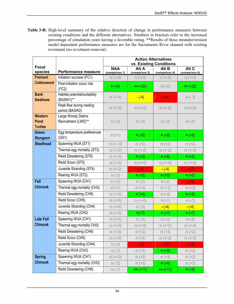
SacEFT Effects Analysis: NODOS
34
Table 3-B: High-level summary of the relative direction of change in performance measures between
existing conditions and the different alternatives. Numbers in brackets refer to the increased
percentage of simulation years having a favorable rating. **Results of these meander/erosion
model dependent performance measures are for the Sacramento River channel with existing
revetment (no revetment removal).
Focal species Performance measure
Action Alternatives vs. Existing Conditions
NAA (comparison 1)
Alt A (comparison 2)
Alt B (comparison 4)
Alt C (comparison 6)
Fremont
Cottonwood
Initiation success (FC1) ni (+/-0) ni (+/-0) ni (+/-0) ni (+/-0)
Post-initiation scour risk
(FC2) + (+9) ++ (+20) ni (+2) ++ (+25)
Bank
Swallows
Habitat potential/suitability
(BASW1)** ni (+/-0) - (-4) - (-5) ni (- 3)
Peak flow during nesting
period (BASW2) ni (+/-0) ni (+/-0) ni (+/-0) ni (+/-0)
Western
Pond
Turtles
Large Woody Debris
Recruitment (LWD)** ni (-3) ni (-3) ni (-3) ni (-3)
Green
Sturgeon
Egg temperature preferences
(GS1) ni (+1) + (+6) + (+8) + (+8)
Steelhead Spawning WUA (ST1) ni (+/- 0) ni (+2) ni (+2) ni (+2)
Thermal egg mortality (ST3) ni (+/-0) ni (+/-0) ni (+/-0) ni (+/-0)
Redd Dewatering (ST6) ni (+/-0) + (+5) + (+6) + (+5)
Redd Scour (ST5) ni (+/-0) ni (+/-0) ni (+/-0) ni (+/-0)
Juvenile Stranding (ST4) ni (+/-0) - (-6) - (-4) - (-7)
Rearing WUA (ST2) ni (-3) + (+5) + (+5) + (+5)
Fall
Chinook
Spawning WUA (CH1) ni (+2) ni (-2) ni (-2) - (-5)
Thermal egg mortality (CH3) ni (+1) ni (+3) ni (+1) ni (+3)
Redd Dewatering (CH6) ni (+/-0) + (+4) ni (+2) + (+4)
Redd Scour (CH5) ni (+/-0) ni (+/-0) ni (-1) ni (-1)
Juvenile Stranding (CH4) ni (+/-0) ni (-3) - (-4) - (-4)
Rearing WUA (CH2) ni (+/-0) +(+7) + (+7) + (+7)
Late Fall
Chinook
Spawning WUA (CH1) ni (+/-0) ni (-3) ni (-3) ni (-3)
Thermal egg mortality CH3) ni (+/-0) ni (+/-0) ni (+/-0) ni (+/-0)
Redd Dewatering (CH6) ni (+/-0) ni (+2) ni (+3) ni (+2)
Redd Scour (CH5) ni (+/-0) ni (+2) ni (+/-0) ni (+/-0)
Juvenile Stranding (CH4) ni (-3) - (-9) - (-6) - (-9)
Rearing WUA (CH2) ni (-1) ni (+3) + (+5) ni (+2)
Spring
Chinook
Spawning WUA (CH1) ni (+/-0) ni (+3) ni (+3) ni (+2)
Thermal egg mortality (CH3) ni (-2) ni (+3) + (+4) ni (+3)
Redd Dewatering (CH6) ni (-1) ++ (+11) ++ (+12) + (+9)

SacEFT Effects Analysis: NODOS
35
Focal species Performance measure
Action Alternatives vs. Existing Conditions
NAA (comparison 1)
Alt A (comparison 2)
Alt B (comparison 4)
Alt C (comparison 6)
Redd Scour (CH5) ni (+2) ni (+/-0) ni (+/-0) ni (+/-0)
Juvenile Stranding (CH4) ni (-1) ni (+2) ni (+2) ni (+2)
Rearing WUA (CH2) ni (+1) - (-8) - (-8) - (-8)
Winter
Chinook
Spawning WUA (CH1) - (-5) ++ (+10) + (+9) ++ (+10)
Thermal egg mortality (CH3) ni (+/-0) ni (+/-0) ni (+/-0) ni (+2)
Redd Dewatering (CH6) ni (-1) + (+4) + (+4) + (+4)
Redd Scour (CH5) ni (+/-0) ni (+/-0) ni (+/-0) ni (+/-0)
Juvenile Stranding (CH4) + (+4) ni (+3) ni (+3) + (+8)
Rearing WUA (CH2) - (-8) - (-4) - (-8) - (-5)
Legend ++
+
ni
-
--
strong beneficial impact owing to project alternative
small beneficial impact owing to project alternative
negligible detected impact owing to project alternative
small negative impact owing to project alternative
strong negative impact owing to project alternative

SacEFT Effects Analysis: NODOS
36
Table 3-C: High-level summary of the relative direction of change in performance measures between
the No Action Alternative and the different alternatives. Numbers in brackets refer to the
increased percentage of simulation years having a favorable rating. **Results of these
meander/erosion model dependent performance measures are for the Sacramento River
channel with existing revetment (no revetment removal).
Focal species Performance measure
Action Alternatives vs. No Action Alternative
Existing (comparison 1)
Alt A (comparison 3)
Alt B (comparison 5)
Alt C (comparison 7)
Fremont
Cottonwood
Initiation success (FC1) ni (+/-0) ni (+/-0) ni (+/-0) ni (+/-0)
Post-initiation scour risk
(FC2) - (-9) ++ (+11) - (-7) ++ (+16)
Bank
Swallows
Habitat potential/suitability
(BASW1)** ni (+/-0) - (-4) - (-5) ni (-3)
Peak flow during nesting
period (BASW2) ni (+/-0) ni (+/-0) ni (+/-0) ni (+/-0)
Western Pond
Turtles
Large Woody Debris
Recruitment (LWD)** ni (+3) ni (+/-0) ni (+/-0) ni (+/-0)
Green
Sturgeon
Egg temperature preferences
(GS1) ni (-1) + (+5) + (+7) + (+7)
Steelhead Spawning WUA (ST1) ni (+/- 0) ni (+2) ni (+2) ni (+2)
Thermal egg mortality (ST3) ni (+/-0) ni (+/-0) ni (+/-0) ni (+/-0)
Redd Dewatering (ST6) ni (+/-0) + (+5) + (+6) + (+5)
Redd Scour (ST5) ni (+/-0) ni (+/-0) ni (+/-0) ni (+/-0)
Juvenile Stranding (ST4) ni (+/-0) - (-6) - (-4) - (-7)
Rearing WUA (ST2) ni (+3) + (+8) + (+8) + (+8)
Fall Chinook Spawning WUA (CH1) ni (-2) - (-4) - (-4) - (-7)
Thermal egg mortality (CH3) ni (-1) ni (+2) ni (+/-0) ni (+2)
Redd Dewatering (CH6) ni (+/-0) + (+4) ni (+2) + (+4)
Redd Scour (CH5) ni (+/-0) ni (+/-0) ni (-1) ni (-1)
Juvenile Stranding (CH4) ni (+/-0) ni (-3) - (-4) - (-4)
Rearing WUA (CH2) ni (+/-0) + (+7) + (+7) + (+7)
Late Fall
Chinook
Spawning WUA (CH1) ni (+/-0) ni (-3) ni (-3) ni (-3)
Thermal egg mortality (CH3) ni (+/-0) ni (+/-0) ni (+/-0) ni (+/-0)
Redd Dewatering (CH6) ni (+/-0) ni (+2) ni (+3) ni (+2)
Redd Scour (CH5) ni (+/-0) ni (+2) ni (+/-0) ni (+/-0)
Juvenile Stranding (CH4) ni (+3) - (-6) ni (-3) - (-6)
Rearing WUA (CH2) ni (+1) + (+4) + (+6) ni (+3)
Spring
Chinook
Spawning WUA (CH1) ni (+/-0) ni (+3) ni (+3) ni (+2)
Thermal egg mortality (CH3) ni (+2) + (+5) + (+6) + (+5)
Redd Dewatering (CH6) ni (+1) ++ (+12) ++ (+13) ++ (+10)
Redd Scour (CH5) ni (-2) ni (-2) ni (-2) ni (-2)
Juvenile Stranding (CH4) ni (+1) ni (+3) ni (+3) ni (+3)
Rearing WUA (CH2) ni (-1) - (-9) - (-9) - (-9)

SacEFT Effects Analysis: NODOS
37
Focal species Performance measure
Action Alternatives vs. No Action Alternative
Existing (comparison 1)
Alt A (comparison 3)
Alt B (comparison 5)
Alt C (comparison 7)
Winter
Chinook
Spawning WUA (CH1) + (+5) ++ (+15) ++ (+14) ++ (+15)
Thermal egg mortality (CH3) ni (+/-0) ni (+/-0) ni (+/-0) ni (+2)
Redd Dewatering (CH6) ni (-1) + (+5) + (+5) + (+5)
Redd Scour (CH5) ni (+/-0) ni (+/-0) ni (+/-0) ni (+/-0)
Juvenile Stranding (CH4) - (-4) ni (-1) ni (-1) + (+4)
Rearing WUA (CH2) + (+8) + (+4) ni (+/-0) ni (+3)
Legend ++
+
ni
-
--
strong beneficial impact owing to project alternative
small beneficial impact owing to project alternative
negligible detected impact owing to project alternative
small negative impact owing to project alternative
strong negative impact owing to project alternative

SacEFT Effects Analysis: NODOS
38
Table 3-D: High-level summary of the relative direction of change in performance measures between the
No Action Alternative (which reflects 2030 conditions, constraints and operations) and
historical flows. Numbers in brackets refer to the increased percentage of simulation years
having a favorable rating. **Results of these meander/erosion model dependent performance
measures are for the Sacramento River channel with existing revetment (no revetment
removal).
Focal species Performance measure
NAA vs.
Historic Conditions (Comparison 8)
Fremont Cottonwood Initiation success (FC1) - - (-17)
Post-initiation scour risk (FC2) ++ (+10)
Bank Swallows Habitat potential/suitability (BASW1)** ni (+1)
Peak flow during nesting period (BASW2) + (+4)
Western Pond Turtles Large Woody Debris Recruitment (LWD)** - - (-29)
Green Sturgeon Egg temperature preferences (GS1) n/a
Steelhead Spawning WUA (ST1) ++ (+14)
Thermal egg mortality (ST3) ni (+/-0)
Redd Dewatering (ST6) + (+9)
Redd Scour (ST5) - - (-16)
Juvenile Stranding (ST4) - - (-24)
Rearing WUA (ST2) ++ (+13)
Fall Chinook Spawning WUA (CH1) - - (-15)
Thermal egg mortality (CH3) + (+8)
Redd Dewatering (CH6) + (+4)
Redd Scour (CH5) - (-5)
Juvenile Stranding (CH4) - - (-25)
Rearing WUA (CH2) ni (+1)
Late Fall Chinook Spawning WUA (CH1) ++ (+11)
Thermal egg mortality (CH3) ni (+/-0)
Redd Dewatering (CH6) + (+6)
Redd Scour (CH5) - - (-13)
Juvenile Stranding (CH4) - - (-11)
Rearing WUA (CH2) ++ (+20)
Spring Chinook Spawning WUA (CH1) ni (-2)
Thermal egg mortality (CH3) + (+8)
Redd Dewatering (CH6) ++ (+35)
Redd Scour (CH5) ni (+/-0)
Juvenile Stranding (CH4) - - (-29)
Rearing WUA (CH2) - - (-13)
Winter Chinook Spawning WUA (CH1) - - (-12)
Thermal egg mortality (CH3) ni (+1)
Redd Dewatering (CH6) ni (-3)
Redd Scour (CH5) - (-5)

SacEFT Effects Analysis: NODOS
39
Focal species Performance measure
NAA vs.
Historic Conditions (Comparison 8)
Juvenile Stranding (CH4) + (+7)
Rearing WUA (CH2) ni (+/-0)
Legend ++
+
ni
-
--
strong beneficial impact owing to project alternative
small beneficial impact owing to project alternative
negligible detected impact owing to project alternative
small negative impact owing to project alternative
strong negative impact owing to project alternative
The purpose of the environmental and feasibility documents is to describe the difference between No
Action / Existing Conditions and the Action Alternatives which all reflect 2030 conditions, constraints
and operations. Typically, none of the NODOS Investigation alternative modelling results are compared
against the historical calibration due to the focus of CEQA/NEPA which emphasizes isolating project
alternative effects as compared to a no action reference or existing condition comparison.
Comparison #8 (see Section 2.5; The NAA, relative to Actual Historic Conditions) is not used in our
report to assess NODOS effects. Instead, it provides an essential reference case illustrating how SacEFT’s
various performance measures have performed under historic flows and water temperatures from 1938 –
2003 relative to the future 2030 conditions, constraints and hydrosystem operations in the NAA. Historic
flows represent less constrained, more natural patterns of variation in flow and water temperature that
have occurred in the past. Comparisons that include historical data reveal different information in a
different context that does not address a specific project effect relative to the no action alternative or
existing condition reference case. These comparisons identify the ecological effects of the future system
operations and constraints relative to historic conditions. In fully considering ecological flow needs, the
magnitude of departure from these historic conditions may reveal important information on how future
constraints, climate and/or hydrosystem operational modifications are influencing preferred ecological
flow targets. Historic flows represent less constrained, more natural patterns of variation in flow and
water temperature that have occurred in the past.
Table 3-D shows that relative to historic flows and water temperatures, conditions associated with the
NAA (comparison 8) generate a strong negative effect on Fremont Cottonwood initiation success (FC1),
Large Woody Debris recruitment (LWD) and Steelhead/fall Chinook/late fall Chinook/spring Chinook
juvenile stranding risk (ST4/CH4). For case #8, fall Chinook spawning WUA (CH1) performance
declined, as it did for winter-run Chinook. Likewise, redd scour risk is increased for Steelhead (ST5) and
late fall Chinook (CH5). Rearing WUA (CH2) habitat conditions were also lower in the case of spring run
Chinook
The following performance measures showed a strong positive effect owing to the NAA relative to actual
historic conditions: Steelhead and late fall Chinook spawning WUA (ST1 and CH1). Also improved were
rearing WUA for late fall Chinook (CH2). Notably, as with NODOS alternatives A, B and C, spring
Chinook redd dewatering risk (CH6) was markedly reduced by conditions present in the NAA vs. actual
historic.

SacEFT Effects Analysis: NODOS
40
3.3 Aquatic Species and Performance Measures
3.3.1 Green Sturgeon
Figure 3.9: Multi-year roll-up results for green sturgeon thermal egg mortality (GS1).
Figure 3.9 and Figure 3.10 show the percentage of years in each NODOS simulation having favorable
(green) conditions for green sturgeon thermal egg mortality (GS1). SacEFT predicts that green sturgeon
eggs (GS1) would receive benefits (+5% to +8% of years with better conditions) from all three of the
NODOS Investigation alternatives in terms of reduction of thermal egg mortality (GS1) (Figure 3.10).
Figure 3.11 shows the number of days in each simulation that water temperatures are above the 20°C lethal threshold for green sturgeon egg development. Consistent with SacEFT preferred condition roll-up
results, the NODOS Investigation alternatives all reduce the number of days green sturgeon eggs are
exposed to lethal water temperatures.
Sacramento Ecological Flows Tool: Green Sturgeon - Egg
Temperature Preferences (GS1); % of simulation years with
favorable conditions
16 5
8 7 8 7
90909090888883
-30
-20
-10
0
10
20
30
40
50
60
70
80
90
100
NAA
Existing
Change
NODOS - Alt A
Existing
Change
NODOS - Alt A
NAA
Change
NODOS - Alt B
Existing
Change
NODOS - Alt B
NAA
Change
NODOS - Alt C
Existing
Change
NODOS - Alt C
NAA
Change
% o
f sim
ula
tion y
ears
Figure 3.10: The percentage of years in each NODOS simulation having favorable (green) conditions
for green sturgeon thermal egg mortality (GS1). Bars labeled with “Change” refer to the %
change between the simulated alternative and the reference condition (either Existing
conditions or the No Action Alternative (NAA)).

SacEFT Effects Analysis: NODOS
41
Sacramento Ecological Flows Tool: Green Sturgeon - Egg
Temperature Preferences (GS1); Days in Simulation Greater
Than 20C; near Hamilton City (~RM199)
-30
-20
-10
0
10
20
30
40
50
60
NAA
Existing
Change
NODOS - Alt A
Existing
Change
NODOS - Alt A
NAA
Change
NODOS - Alt B
Existing
Change
NODOS - Alt B
NAA
Change
NODOS - Alt C
Existing
Change
NODOS - Alt C
NAA
Change
Days G
reate
r Than 2
0C
Figure 3.11: Number of days in each simulation where water temperatures near Hamilton City (RM199)
are greater than 20°C. Bars labeled with “Change” refer to the change in number of days greater than 20°C between the simulated alternative and the reference condition (either Existing conditions or the No Action Alternative (NAA)).
SacEFT Target and Avoidance Flows for Green Sturgeon Egg Development
Figure 3.12 shows the SacEFT target/favorable water temperature profiles and the median target water
temperature at the Sacramento River near Red Bluff (RM260) and Hamilton City (RM199) during the
critical period for green sturgeon egg development.

SacEFT Effects Analysis: NODOS
42
SacEFT: Target/Favourable Water Temperature Profiles
(Sacramento River nr Red Bluff; ~RM260) during Green Sturgeon
Critical Period (Mar-1 to Aug-15)
17C
20C
1977
6789
1011121314151617181920212223
'Oct-01
'Oct-08
'Oct-15
'Oct-22
'Oct-29
'Nov
-05
'Nov
-12
'Nov
-19
'Nov
-26
'Dec
-03
'Dec
-10
'Dec
-17
'Dec
-24
'Dec
-31
'Jan
-07
'Jan
-14
'Jan
-21
'Jan
-28
'Feb
-04
'Feb
-11
'Feb
-18
'Feb
-25
'Mar-03
'Mar-10
'Mar-17
'Mar-24
'Mar-31
'Apr-07
'Apr-14
'Apr-21
'Apr-28
'May
-05
'May
-12
'May
-19
'May
-26
'Jun
-02
'Jun
-09
'Jun
-16
'Jun
-23
'Jun
-30
'Jul-07
'Jul-14
'Jul-21
'Jul-28
'Aug
-04
'Aug
-11
'Aug
-18
'Aug
-25
'Sep
-01
'Sep
-08
'Sep
-15
'Sep
-22
'Sep
-29
Wa
ter
Te
mp
era
ture
(C
elc
ius)
SacEFT: Target/Favourable Water Temperature Profiles
(Sacramento River nr Hamilton City; ~RM199) during Green
Sturgeon Critical Period (Mar-1 to Aug-15)
17C
20C
6789
1011121314151617181920212223
'Oct-01
'Oct-08
'Oct-15
'Oct-22
'Oct-29
'Nov
-05
'Nov
-12
'Nov
-19
'Nov
-26
'Dec
-03
'Dec
-10
'Dec
-17
'Dec
-24
'Dec
-31
'Jan
-07
'Jan
-14
'Jan
-21
'Jan
-28
'Feb
-04
'Feb
-11
'Feb
-18
'Feb
-25
'Mar-03
'Mar-10
'Mar-17
'Mar-24
'Mar-31
'Apr-07
'Apr-14
'Apr-21
'Apr-28
'May
-05
'May
-12
'May
-19
'May
-26
'Jun
-02
'Jun
-09
'Jun
-16
'Jun
-23
'Jun
-30
'Jul-07
'Jul-14
'Jul-21
'Jul-28
'Aug
-04
'Aug
-11
'Aug
-18
'Aug
-25
'Sep
-01
'Sep
-08
'Sep
-15
'Sep
-22
'Sep
-29
Wa
ter
Te
mp
era
ture
(C
elc
ius)
Figure 3.12: Target/favorable water temperature profiles (green) for minimizing green sturgeon thermal egg
mortality (GS1) at two index locations (RM260 and RM199). Water temperature profiles in green
refer to years where SacEFT’s annual performance measure rating was assessed as good/favorable.
The heavy black line provides the median of the all year favorable water temperature profiles. Lines
in red show example years rated as poor by SacEFT (i.e., highest category of egg mortality).
Horizontal lines at 17°C and 20°C are important thresholds that affect green sturgeon egg development (GS1). [Note: this figure is designed for color printing].
Figure 3.13 provides an example of detailed daily output available from SacEFT for a poor year like
1977.

SacEFT Effects Analysis: NODOS
43
Scenario:
Water year:
Location of interest:
Units Celsius
1977
ACTUAL HISTORICAL CONDITIONS (FROM OBSERVED STREAM TEMPERATURE MEASUREMENTS)
GS1 - Site 1 - Hamilton City
4
8
12
16
20
24
1-M
ar
8-M
ar
15-M
ar
22-M
ar
29-M
ar
5-Apr
12-Apr
19-Apr
26-Apr
3-M
ay
10-M
ay
17-M
ay
24-M
ay
31-M
ay
7-Jun
14-Jun
21-Jun
28-Jun
5-Jul
12-Jul
19-Jul
26-Jul
2-Aug
9-Aug
Period of Interest
Temperature (C)
Good/Fair Threshold
Fair/Poor Threshold
Water Temperature
SacEFT - Green Sturgeon Egg Hazard Report
0
0.2
0.4
0.6
0.8
1
1.2
1-M
ar
8-M
ar
15-M
ar
22-M
ar
29-M
ar
5-Apr
12-Apr
19-Apr
26-Apr
3-M
ay
10-M
ay
17-M
ay
24-M
ay
31-M
ay
7-Jun
14-Jun
21-Jun
28-Jun
5-Jul
12-Jul
19-Jul
26-Jul
2-Aug
9-Aug
Period of Interest
Daily Mortality
0
0.05
0.1
0.15
0.2
0.25
0.3
Cumulative Mortality
Distribution
Daily Mortality
Good
Fair
Bad
Cumulative Mortality
Figure 3.13: SacEFT detailed output report for a specific water year (1977) showing daily results for green
sturgeon thermal egg mortality (GS1) at a specific index location (Hamilton City).
3.3.2 Steelhead Trout
Figure 3.14 to Figure 3.18 show the percentage of years in each NODOS simulation having favorable
(green) conditions for the six independent Steelhead trout performance measure in SacEFT (ST3 omitted
as SacEFT rates all scenarios as 100% favorable). SacEFT predicts that Steelhead would receive benefits
in terms of reduced redd dewatering (ST6) (+5% to +6% of years with better conditions) from all three of
the NODOS Investigation alternatives (Figure 3.15) as well as improvements to rearing conditions (ST2)
(+5% to +8% of years with more favorable conditions) (Figure 3.18). Conversely the NODOS

SacEFT Effects Analysis: NODOS
44
Investigation alternatives increase juvenile stranding risks (ST4) over both existing conditions and NAA
(approx. –4% to –7% reduction in years with favorable conditions) (Figure 3.17). Stranding risk increases
(ST4) are particularly apparent when compared to rates of stranding found with historical flows (Figure
3.17). Likewise, redd scour risks are higher in all NODOS alternatives relative to historic conditions
(Figure 3.16).
Sacramento Ecological Flows Tool: Steelhead - Spawning WUA (ST1); %
of simulation years with favorable conditions
02 2 2 2 2 2
52
38
14
54545454545452
-30
-20
-10
0
10
20
30
40
50
60
NAA
Existing
Change
NODOS - Alt A
Existing
Change
NODOS - Alt A
NAA
Change
NODOS - Alt B
Existing
Change
NODOS - Alt B
NAA
Change
NODOS - Alt C
Existing
Change
NODOS - Alt C
NAA
Change
NAA
HIST.
Change
% o
f sim
ula
tion y
ears
Figure 3.14: The percentage of years in each NODOS simulation having favorable (green) conditions
for Steelhead spawning WUA (ST1). Bars labeled with “Change” refer to the % change
between the simulated alternative and the reference condition (either Existing conditions or
the No Action Alternative (NAA)).
Sacramento Ecological Flows Tool: Steelhead - Redd Dewatering (ST6);
% of simulation years with favorable conditions
05 5 6 6 5 5
51
42
9
5156 56 57 57 56 56
-30
-20
-10
0
10
20
30
40
50
60
70
NAA
Existing
Change
NODOS - Alt A
Existing
Change
NODOS - Alt A
NAA
Change
NODOS - Alt B
Existing
Change
NODOS - Alt B
NAA
Change
NODOS - Alt C
Existing
Change
NODOS - Alt C
NAA
Change
NAA
HIST.
Change
% o
f sim
ula
tion y
ears
Figure 3.15: The percentage of years in each NODOS simulation having favorable (green) conditions
for Steelhead redd dewatering (ST6). Bars labeled with “Change” refer to the % change
between the simulated alternative and the reference condition (either Existing conditions or
the No Action Alternative (NAA)).

SacEFT Effects Analysis: NODOS
45
Sacramento Ecological Flows Tool: Steelhead - Redd Scour (ST5); % of
simulation years with favorable conditions
0 0 0 0 0 0 0
62
78
62626262626262
-16
-30
-20
-10
0
10
20
30
40
50
60
70
80
90
NAA
Existing
Change
NODOS - Alt A
Existing
Change
NODOS - Alt A
NAA
Change
NODOS - Alt B
Existing
Change
NODOS - Alt B
NAA
Change
NODOS - Alt C
Existing
Change
NODOS - Alt C
NAA
Change
NAA
HIST.
Change
% o
f sim
ula
tion y
ears
Figure 3.16: The percentage of years in each NODOS simulation having favorable (green) conditions
for Steelhead redd scour (ST5). Bars labeled with “Change” refer to the % change between
the simulated alternative and the reference condition (either Existing conditions or the No
Action Alternative (NAA)).
Sacramento Ecological Flows Tool: Steelhead - Juvenile Stranding
(ST4); % of simulation years with favorable conditions
0
9
33
2255
33
9
-24-6 -6 -4 -4 -7 -7
-30
-20
-10
0
10
20
30
40
NAA
Existing
Change
NODOS - Alt A
Existing
Change
NODOS - Alt A
NAA
Change
NODOS - Alt B
Existing
Change
NODOS - Alt B
NAA
Change
NODOS - Alt C
Existing
Change
NODOS - Alt C
NAA
Change
NAA
HIST.
Change%
of sim
ula
tion y
ears
Figure 3.17: The percentage of years in each NODOS simulation having favorable (green) conditions
for Steelhead juvenile stranding (ST4). Bars labeled with “Change” refer to the % change
between the simulated alternative and the reference condition (either Existing conditions or
the No Action Alternative (NAA)).

SacEFT Effects Analysis: NODOS
46
Sacramento Ecological Flows Tool: Steelhead - Rearing WUA (ST2); %
of simulation years with favorable conditions
58
58
58
46
33
13
545454545454
46
-3
-30
-20
-10
0
10
20
30
40
50
60
NAA
Existing
Change
NODOS - Alt A
Existing
Change
NODOS - Alt A
NAA
Change
NODOS - Alt B
Existing
Change
NODOS - Alt B
NAA
Change
NODOS - Alt C
Existing
Change
NODOS - Alt C
NAA
Change
NAA
HIST.
Change
% o
f sim
ula
tion y
ears
Figure 3.18: The percentage of years in each NODOS simulation having favorable (green) conditions
for Steelhead rearing WUA (ST2). Bars labeled with “Change” refer to the % change
between the simulated alternative and the reference condition (either Existing conditions or
the No Action Alternative (NAA)).
Readers are referred to Appendix C for raw data for the results presented above, as well as all relevant
SacEFT multi-year roll-up screen shot images.

SacEFT Effects Analysis: NODOS
47
SacEFT Target and Avoidance Flows and Water Temperatures for Steelhead Trout
Figure 3.19 shows the SacEFT target/favorable flow profiles and the median target flow at the
Sacramento River near Red Bluff (RM260) during the critical period for Steelhead trout spawning as
found using the spawning WUA performance measure (ST1).
(a)
SacEFT: Target/Favourable Flow Profiles (Sacramento River
nr Red Bluff; ~RM260) during Critical Period for Steelhead
Spawning (Nov-16 to May-15)
6,779
0
20000
40000
60000
80000
100000
120000'O
ct-01
'Oct-08
'Oct-15
'Oct-22
'Oct-29
'Nov-05
'Nov-12
'Nov-19
'Nov-26
'Dec-03
'Dec-10
'Dec-17
'Dec-24
'Dec-31
'Jan-07
'Jan-14
'Jan-21
'Jan-28
'Feb-04
'Feb-11
'Feb-18
'Feb-25
'Mar-03
'Mar-10
'Mar-17
'Mar-24
'Mar-31
'Apr-07
'Apr-14
'Apr-21
'Apr-28
'May-05
'May-12
'May-19
'May-26
'Jun-02
'Jun-09
'Jun-16
'Jun-23
'Jun-30
'Jul-07
'Jul-14
'Jul-21
'Jul-28
'Aug-04
'Aug-11
'Aug-18
'Aug-25
'Sep-01
'Sep-08
'Sep-15
'Sep-22
'Sep-29
Dis
cha
rge
(cf
s)
(b)
SacEFT: Example Avoidance Flow Profiles (Sacramento River
nr. Red Bluf; ~RM260) from NODOS Alt. A during Critical
Period for Steelhead Spawning (Nov-16 to May-15)
0
20000
40000
60000
80000
100000
120000
'Oct-01
'Oct-08
'Oct-15
'Oct-22
'Oct-29
'Nov
-05
'Nov
-12
'Nov
-19
'Nov
-26
'Dec
-03
'Dec
-10
'Dec
-17
'Dec
-24
'Dec
-31
'Jan
-07
'Jan
-14
'Jan
-21
'Jan
-28
'Feb
-04
'Feb
-11
'Feb
-18
'Feb
-25
'Mar-03
'Mar-10
'Mar-17
'Mar-24
'Mar-31
'Apr-07
'Apr-14
'Apr-21
'Apr-28
'May
-05
'May
-12
'May
-19
'May
-26
'Jun
-02
'Jun
-09
'Jun
-16
'Jun
-23
'Jun
-30
'Jul-0
7'Jul-1
4'Jul-2
1'Jul-2
8'Aug
-04
'Aug
-11
'Aug
-18
'Aug
-25
'Sep
-01
'Sep
-08
'Sep
-15
'Sep
-22
'Sep
-29
Dis
cha
rge
(cf
s)
Figure 3.19: Target/favorable flow profiles (green) for steelhead spawning WUA (ST1) at Sacramento River near Red
Bluff (RM260). Flow profiles in green refer to years where SacEFT’s annual performance measure rating
was assessed as good/favorable. The heavy black line provides the median of the all year favorable flow
profiles. The grey horizontal line (panel a) is the average of the median target flow. Flow traces in red
(panel b) are examples of typical years rated poor by SacEFT (i.e., least cumulative spawning habitat
potential). [Note: this figure is designed for color printing].

SacEFT Effects Analysis: NODOS
48
Figure 3.20 shows the SacEFT target/favorable flow profiles and the median target flow at the
Sacramento River near Red Bluff (RM260) during the critical period for Steelhead trout egg incubation as
found using the redd dewatering performance measure (ST6).
(a)
SacEFT: Target/Favourable Flow Profiles (Sacramento River
nr Red Bluff; ~RM260) during Critical Period for Steelhead
Egg Incubation (Nov-16 to May-15)
7,19375th percentile (good years)
75th percentile poor years
0
20000
40000
60000
80000
100000
120000'O
ct-01
'Oct-08
'Oct-15
'Oct-22
'Oct-29
'Nov-05
'Nov-12
'Nov-19
'Nov-26
'Dec-03
'Dec-10
'Dec-17
'Dec-24
'Dec-31
'Jan-07
'Jan-14
'Jan-21
'Jan-28
'Feb-04
'Feb-11
'Feb-18
'Feb-25
'Mar-03
'Mar-10
'Mar-17
'Mar-24
'Mar-31
'Apr-07
'Apr-14
'Apr-21
'Apr-28
'May-05
'May-12
'May-19
'May-26
'Jun-02
'Jun-09
'Jun-16
'Jun-23
'Jun-30
'Jul-07
'Jul-14
'Jul-21
'Jul-28
'Aug-04
'Aug-11
'Aug-18
'Aug-25
'Sep-01
'Sep-08
'Sep-15
'Sep-22
'Sep-29
Dis
cha
rge
(cf
s)
(b)
SacEFT: Example Avoidance Flow Profiles (Sacramento River
nr. Red Bluf; ~RM260) from NODOS Existing during Critical
Period for Steelhead Egg Incubation (Nov-16 to May-15)
0
20000
40000
60000
80000
100000
120000
'Oct-01
'Oct-08
'Oct-15
'Oct-22
'Oct-29
'Nov-05
'Nov-12
'Nov-19
'Nov-26
'Dec-03
'Dec-10
'Dec-17
'Dec-24
'Dec-31
'Jan-07
'Jan-14
'Jan-21
'Jan-28
'Feb-04
'Feb-11
'Feb-18
'Feb-25
'Mar-03
'Mar-10
'Mar-17
'Mar-24
'Mar-31
'Apr-07
'Apr-14
'Apr-21
'Apr-28
'May-05
'May-12
'May-19
'May-26
'Jun-02
'Jun-09
'Jun-16
'Jun-23
'Jun-30
'Jul-07
'Jul-14
'Jul-21
'Jul-28
'Aug-04
'Aug-11
'Aug-18
'Aug-25
'Sep-01
'Sep-08
'Sep-15
'Sep-22
'Sep-29
Dis
cha
rge
(cf
s)
Figure 3.20: Example target/favorable flow profiles (green) for steelhead redd dewatering (ST6) at Sacramento
River near Red Bluff (RM260) (panel a). Flow profiles in green refer to years where SacEFT’s
annual performance measure rating was assessed as good/favorable. Example flow traces in red
(panel b) are examples of typical years rated poor by SacEFT (i.e., highest values of redd
dewatering).

SacEFT Effects Analysis: NODOS
49
Steelheed redd de-watering risk is driven primarily by the presence of high flows during spawning, which
contributes to a higher percentage of redds being spawned at higher elevations. This is apparent when
comparing the 75th percentile flows between low de-watering years and high de-watering years in panel a
of Figure 3.20. Hence, the de-watering threshold is dynamic, and will be higher the higher average flows
during the steelhead spawning period.
Figure 3.21 shows the SacEFT target/favorable flow profiles and the median target flow at the
Sacramento River near Red Bluff (RM260) during the critical period for Steelhead trout egg incubation as
found using the redd scour performance measure (ST5).
Figure 3.22 shows the SacEFT target/favorable flow profiles and the median target flow at the
Sacramento River near Red Bluff (RM260) during the critical period for Steelhead trout juvenile rearing
as found using the juvenile stranding performance measure (ST4).
Figure 3.23 shows the SacEFT target/favorable flow profiles and the median target flow at the
Sacramento River near Red Bluff (RM260) during the critical period for Steelhead trout juvenile rearing
as found using the juvenile rearing WUA performance measure (ST2).

SacEFT Effects Analysis: NODOS
50
(a)
SacEFT: Target/Favourable Flow Profiles (Sacramento River
nr Red Bluff; ~RM260) to limit Redd Scour during Critical
Period for Steelhead Egg Incubation (Nov-16 to May-15)
55,000
75,000
0
20000
40000
60000
80000
100000
120000
140000
160000
'Oct-01
'Oct-08
'Oct-15
'Oct-22
'Oct-29
'Nov-05
'Nov-12
'Nov-19
'Nov-26
'Dec-03
'Dec-10
'Dec-17
'Dec-24
'Dec-31
'Jan-07
'Jan-14
'Jan-21
'Jan-28
'Feb-04
'Feb-11
'Feb-18
'Feb-25
'Mar-03
'Mar-10
'Mar-17
'Mar-24
'Mar-31
'Apr-07
'Apr-14
'Apr-21
'Apr-28
'May-05
'May-12
'May-19
'May-26
'Jun-02
'Jun-09
'Jun-16
'Jun-23
'Jun-30
'Jul-07
'Jul-14
'Jul-21
'Jul-28
'Aug-04
'Aug-11
'Aug-18
'Aug-25
'Sep-01
'Sep-08
'Sep-15
'Sep-22
'Sep-29
Dis
cha
rge
(cf
s)
(b)
SacEFT: Example Redd Scour Avoidance Flow Profiles
(Sacramento River nr. Red Bluf; ~RM260) during Critical
Period for Steelhead Egg Incubation (Nov-16 to May-15)
55,000
75,000
0
20000
40000
60000
80000
100000
120000
140000
160000
'Oct-01
'Oct-08
'Oct-15
'Oct-22
'Oct-29
'Nov-05
'Nov-12
'Nov-19
'Nov-26
'Dec-03
'Dec-10
'Dec-17
'Dec-24
'Dec-31
'Jan-07
'Jan-14
'Jan-21
'Jan-28
'Feb-04
'Feb-11
'Feb-18
'Feb-25
'Mar-03
'Mar-10
'Mar-17
'Mar-24
'Mar-31
'Apr-07
'Apr-14
'Apr-21
'Apr-28
'May-05
'May-12
'May-19
'May-26
'Jun-02
'Jun-09
'Jun-16
'Jun-23
'Jun-30
'Jul-07
'Jul-14
'Jul-21
'Jul-28
'Aug-04
'Aug-11
'Aug-18
'Aug-25
'Sep-01
'Sep-08
'Sep-15
'Sep-22
'Sep-29
Dis
cha
rge
(cf
s)
Figure 3.21: Target/favorable flow profiles (green) for minimizing steelhead egg scour mortality (ST5) at
Sacramento River near Red Bluff (RM260) (panel a). Flow profiles in green refer to years where
SacEFT’s annual performance measure rating was assessed as good/favorable. The heavy black line
(panel a) provides the median of the all year favorable flow profiles. Example flow traces in red
(panel b) are examples of typical years rated poor by SacEFT (i.e., highest values of redd scour).
Horizontal lines at 55,000 cfs and 75,000 cfs are important thresholds that affect steelhead egg scour
mortality rates (ST5).

SacEFT Effects Analysis: NODOS
51
(a)
SacEFT: Target/Favourable Flow Profiles (Sacramento River
nr Red Bluff; ~RM260) during Critical Period for Steelhead
Juvenile Stranding (year round)
0
20000
40000
60000
80000
100000
120000
140000
160000
'Oct-01
'Oct-08
'Oct-15
'Oct-22
'Oct-29
'Nov-05
'Nov-12
'Nov-19
'Nov-26
'Dec-03
'Dec-10
'Dec-17
'Dec-24
'Dec-31
'Jan-07
'Jan-14
'Jan-21
'Jan-28
'Feb-04
'Feb-11
'Feb-18
'Feb-25
'Mar-03
'Mar-10
'Mar-17
'Mar-24
'Mar-31
'Apr-07
'Apr-14
'Apr-21
'Apr-28
'May-05
'May-12
'May-19
'May-26
'Jun-02
'Jun-09
'Jun-16
'Jun-23
'Jun-30
'Jul-07
'Jul-14
'Jul-21
'Jul-28
'Aug-04
'Aug-11
'Aug-18
'Aug-25
'Sep-01
'Sep-08
'Sep-15
'Sep-22
'Sep-29
Dis
cha
rge
(cf
s)
(b)
SacEFT: Example Avoidance Flow Profiles (Sacramento River
nr Red Bluff; ~RM260) from NODOS Existing during Critical
Period for Steelhead Juvenile Stranding (year round)
Avg of median
of poor yrs
Avg of median
of good yrs
3000
4000
5000
6000
7000
8000
9000
10000
11000
12000
13000
14000
'Oct-01
'Oct-08
'Oct-15
'Oct-22
'Oct-29
'Nov-05
'Nov-12
'Nov-19
'Nov-26
'Dec-03
'Dec-10
'Dec-17
'Dec-24
'Dec-31
'Jan-07
'Jan-14
'Jan-21
'Jan-28
'Feb-04
'Feb-11
'Feb-18
'Feb-25
'Mar-03
'Mar-10
'Mar-17
'Mar-24
'Mar-31
'Apr-07
'Apr-14
'Apr-21
'Apr-28
'May-05
'May-12
'May-19
'May-26
'Jun-02
'Jun-09
'Jun-16
'Jun-23
'Jun-30
'Jul-07
'Jul-14
'Jul-21
'Jul-28
'Aug-04
'Aug-11
'Aug-18
'Aug-25
'Sep-01
'Sep-08
'Sep-15
'Sep-22
'Sep-29
Dis
cha
rge
(cf
s)
Figure 3.22: Target/favorable flow profiles (green) for minimizing juvenile steelhead stranding mortality (ST4) at
Sacramento River near Red Bluff (RM260) (panel a). Flow profiles in green refer to years where
SacEFT’s annual performance measure rating was assessed as good/favorable. The heavy black line
(panel a) provides the median of the all year favorable flow profiles. Example flow traces in red
(panel b) are examples of typical years rated poor by SacEFT (i.e., highest values of juvenile
stranding). [Note: this figure is designed for color printing].

SacEFT Effects Analysis: NODOS
52
(a)
SacEFT: Target/Favourable Flow Profiles (Sacramento River
nr Red Bluff; ~RM260) during Critical Period for Steelhead
Juvenile Rearing WUA (year round)
75th percentile good
yrs
75th percentile poor
yrs
0
20000
40000
60000
80000
100000
120000
140000
160000
'Oct-01
'Oct-08
'Oct-15
'Oct-22
'Oct-29
'Nov-05
'Nov-12
'Nov-19
'Nov-26
'Dec-03
'Dec-10
'Dec-17
'Dec-24
'Dec-31
'Jan-07
'Jan-14
'Jan-21
'Jan-28
'Feb-04
'Feb-11
'Feb-18
'Feb-25
'Mar-03
'Mar-10
'Mar-17
'Mar-24
'Mar-31
'Apr-07
'Apr-14
'Apr-21
'Apr-28
'May-05
'May-12
'May-19
'May-26
'Jun-02
'Jun-09
'Jun-16
'Jun-23
'Jun-30
'Jul-07
'Jul-14
'Jul-21
'Jul-28
'Aug-04
'Aug-11
'Aug-18
'Aug-25
'Sep-01
'Sep-08
'Sep-15
'Sep-22
'Sep-29
Dis
cha
rge
(cf
s)
(b)
SacEFT: Example Avoidance Flow Profiles (Sacramento River
nr Red Bluff; ~RM260) from NODOS Existing during Critical
Period for Steelhead Juvenile Rearing WUA (year round)
0
20000
40000
60000
80000
100000
120000
140000
160000
'Oct-01
'Oct-08
'Oct-15
'Oct-22
'Oct-29
'Nov-05
'Nov-12
'Nov-19
'Nov-26
'Dec-03
'Dec-10
'Dec-17
'Dec-24
'Dec-31
'Jan-07
'Jan-14
'Jan-21
'Jan-28
'Feb-04
'Feb-11
'Feb-18
'Feb-25
'Mar-03
'Mar-10
'Mar-17
'Mar-24
'Mar-31
'Apr-07
'Apr-14
'Apr-21
'Apr-28
'May-05
'May-12
'May-19
'May-26
'Jun-02
'Jun-09
'Jun-16
'Jun-23
'Jun-30
'Jul-07
'Jul-14
'Jul-21
'Jul-28
'Aug-04
'Aug-11
'Aug-18
'Aug-25
'Sep-01
'Sep-08
'Sep-15
'Sep-22
'Sep-29
Dis
cha
rge
(cf
s)
Figure 3.23: Target/favorable flow profiles (green) for maximizing juvenile steelhead rearing WUA (ST2) at
Sacramento River near Red Bluff (RM260) (panel a). Flow profiles in green refer to years where
SacEFT’s annual performance measure rating was assessed as good/favorable. The heavy black line
(panel a) provides the median of the all year favorable flow profiles. Example flow traces in red
(panel b) are examples of typical years rated poor by SacEFT (i.e., poorest values for juvenile
rearing WUA). [Note: this figure is designed for color printing].

SacEFT Effects Analysis: NODOS
53
3.3.3 Fall Chinook
Readers are referred to Appendix C (FALL Chinook worksheet) for fall Chinook results for the six
independent salmonid performance measures in SacEFT (CH1, CH3, CH6, CH5, CH4, CH2).
Section 3.2 summarizes the performance of the NODOS alternatives for fall Chinook (Table 3-B).
Using the same methods applied to Steelhead trout, it is possible to use SacEFT to quantify target and
avoidance flows at index locations for fall Chinook critical periods.
3.3.4 Late Fall Chinook
Readers are referred to Appendix C (LFALL Chinook worksheet) for late fall Chinook results for the six
independent salmonid performance measures in SacEFT (CH1, CH3, CH6, CH5, CH4, CH2).
Section 3.2 summarizes the performance of the NODOS alternatives for late fall Chinook (Table 3-B).
Using the same methods applied to Steelhead trout, it is possible to use SacEFT to quantify target and
avoidance flows at index locations for late-fall Chinook critical periods.
3.3.5 Spring Chinook
Readers are referred to Appendix C (SPRING Chinook worksheet) for late fall Chinook results for the six
independent salmonid performance measures in SacEFT (CH1, CH3, CH6, CH5, CH4, CH2).
Section 3.2 summarizes the performance of the NODOS alternatives for spring Chinook (Table 3-B).
Using the same methods applied to Steelhead trout, it is possible to use SacEFT to quantify target and
avoidance flows at index locations for spring Chinook critical periods.
3.3.6 Winter Chinook
Readers are referred to Appendix C (WINTER Chinook worksheet) for winter-run Chinook results for the
six independent salmonid performance measures in SacEFT (CH1, CH3, CH6, CH5, CH4, CH2).
Section 3.2 summarizes the performance of the NODOS alternatives for winter-run Chinook (Table 3-B).
Using the same methods applied to Steelhead trout, it is possible to use SacEFT to quantify target and
avoidance flows at index locations for winter-run Chinook critical periods.

SacEFT Effects Analysis: NODOS
54
3.4 Riparian Species and Performance measures
3.4.1 Fremont Cottonwood Initiation
Figure 3.24: Multi-year roll-up results for Fremont cottonwood seedling initiation success (FC1).
Figure 3.24 and Figure 3.25 show the percentage of years in each NODOS simulation having favorable
(green) conditions for Fremont cottonwood seedling initiation (FC1). SacEFT predicts that Fremont
cottonwood initiation (FC1) would not be impacted by any of the NODOS Investigation alternatives
when compared with the existing conditions or NAA (Figure 3.25). However, results indicate that all of
the NODOS alternatives are expected to generate unfavorable Cottonwood initiation conditions.
Sacramento Ecological Flows Tool: Fremont Cottonwood - Initiation
Success (FC1); % of simulation years with favorable conditions
0 0 0 0 0 0 0 0
17
-17
0000000
-30
-20
-10
0
10
20
NAA
Existing
Change
NODOS - Alt A
Existing
Change
NODOS - Alt A
NAA
Change
NODOS - Alt B
Existing
Change
NODOS - Alt B
NAA
Change
NODOS - Alt C
Existing
Change
NODOS - Alt C
NAA
Change
NAA
HIST.
Change
% o
f sim
ula
tion y
ears
Figure 3.25: The percentage of years in each NODOS simulation having favorable (green) conditions
for Fremont cottonwood seedling initiation (FC1). Bars labeled with “Change” refer to the
% change between the simulated alternative and the reference condition (either Existing
conditions or the No Action Alternative (NAA)).
It is noted that scour risk (FC2) is reduced under the NODOS alternatives, especially alternative C and A
(Figure 3.26). However, this reduction in scour risk is in part due to the reduction in number of years with
successful initiation (FC1). The FC2 performance measure in SacEFT is only relevant/calculated in years
with successful Fremont cottonwood initiation (FC1).

SacEFT Effects Analysis: NODOS
55
Sacramento Ecological Flows Tool: Fremont Cottonwood - Post-initiation
Scour Risk (FC2); % of simulation years with favorable conditions
9
20
11
2
25
16
64
54
10
8080
5757
7575
64
-7
-30
-20
-10
0
10
20
30
40
50
60
70
80
90
NAA
Existing
Change
NODOS - Alt A
Existing
Change
NODOS - Alt A
NAA
Change
NODOS - Alt B
Existing
Change
NODOS - Alt B
NAA
Change
NODOS - Alt C
Existing
Change
NODOS - Alt C
NAA
Change
NAA
HIST.
Change
% o
f sim
ula
tion y
ears
Figure 3.26: The percentage of years in each NODOS simulation having favorable (green) conditions
for Fremont cottonwood seedling scour (FC2). Bars labeled with “Change” refer to the %
change between the simulated alternative and the reference condition (either Existing
conditions or the No Action Alternative (NAA)). Note: The FC2 performance measure in
SacEFT is only relevant/calculated in years with successful Fremont cottonwood initiation
(FC1).
In terms of Fremont cottonwood initiation, all NODOS alternative flows eliminate strong initiation events
(see Figure 3.27).

SacEFT Effects Analysis: NODOS
56
(a) Scenario: VERSION 2 CALIBRATION RUN (HISTORICAL)
SacEFT - Riparian Initiation Multi-year Report
0
20
40
60
80
100
120
1983
1958
1941
1969
2003
1998
1956
1982
2004
1963
1973
1999
1980
1965
1989
1993
1976
1957
1970
1988
1946
1979
1961
1960
1986
1985
1964
1949
1962
1948
1945
1950
1944
Water Year
# nodes w
surviving
cottonwoods over
all cross sections
(b) Scenario: NODOS - Existing, NoRipRapRemoval
SacEFT - Riparian Initiation Multi-year Report
0
20
40
60
80
100
120
1967
1938
1952
1977
1993
1971
1996
1988
1969
1999
1960
1986
1923
1943
1994
2002
1956
1980
1954
1974
1985
1997
1948
1995
1929
1970
1989
1963
1982
1962
1935
1939
1947
1951
1990
1936
1964
1945
1930
Water Year
# nodes w
surviving
cottonwoods over
all cross sections
(c) Scenario: NODOS - Alternative A, NoRipRapRemoval
SacEFT - Riparian Initiation Multi-year Report
0
20
40
60
80
100
120
1983
1967
1992
1975
1977
1934
1938
1981
2003
1986
1927
1978
1940
1971
1990
1929
1943
1946
1960
1931
1954
1965
1980
1951
1972
1942
1948
1963
1955
1989
1996
1925
1959
1998
1926
1944
1932
1950
1991
Water Year
# nodes w
surviving
cottonwoods over
all cross sections
(d) Scenario: NODOS - Alternative B, NoRipRapRemoval
SacEFT - Riparian Initiation Multi-year Report
0
20
40
60
80
100
120
1983
1941
1969
1931
1988
2001
2003
1987
1993
1971
1981
1984
1934
1954
1970
2000
1937
1968
1940
1948
1956
1980
1927
1978
1996
1979
1925
1936
1966
1945
1951
1923
1933
1962
1985
1955
1947
1964
1924
Water Year
# nodes w
surviving
cottonwoods over
all cross sections
(e) Scenario: NODOS - Alternative C, NoRipRapRemoval
SacEFT - Riparian Initiation Multi-year Report
0
20
40
60
80
100
120
1983
1967
1992
1975
1987
1938
1927
1978
1988
1923
1937
1969
1982
1945
1956
1977
1984
1926
1933
1961
1989
2000
1963
1965
1972
1980
1942
1957
1949
1959
1948
1996
2002
1974
1936
1962
1932
1997
1950
Water Year
# nodes w
surviving
cottonwoods over
all cross sections
Figure 3.27: Annual index of total number of SacEFT cross-section nodes (entire study area) with successfully
initiating Fremont cottonwood seedlings (FC1). These annual results are sorted in descending order.
Panel (a) shows results for historical flows from 1938 to 2004. Green shaded bars refer to initiation
totals that if met or exceeded, receive a favorable (green) rating in SacEFT. Panel (b) is for the
NODOS existing conditions alternative. Panel (c) gives results for NODOS Investigation alternative
A. Panel (d) shows results for NODOS Investigation alternative B. Finally, panel (e) shows results
for NODOS Investigation alternative C.

SacEFT Effects Analysis: NODOS
57
Figure 3.28, Figure 3.29 and Figure 3.30 show the SacEFT target/favorable flow profiles and target flow
recession rate at several index locations along the Sacramento River during the critical period for Fremont
cottonwood seedling initiation (FC1).
SacEFT: Target/Favourable Flow Profiles (Sacramento River
nr Bend Bridge; ~RM260) during Critical Period for
Cottonwood Initiation (Apr-15 to Jul-31)
0
10000
20000
30000
40000
50000
60000
70000
80000
90000
'Oct-01
'Oct-08
'Oct-15
'Oct-22
'Oct-29
'Nov-05
'Nov-12
'Nov-19
'Nov-26
'Dec-03
'Dec-10
'Dec-17
'Dec-24
'Dec-31
'Jan-07
'Jan-14
'Jan-21
'Jan-28
'Feb-04
'Feb-11
'Feb-18
'Feb-25
'Mar-03
'Mar-10
'Mar-17
'Mar-24
'Mar-31
'Apr-07
'Apr-14
'Apr-21
'Apr-28
'May-05
'May-12
'May-19
'May-26
'Jun-02
'Jun-09
'Jun-16
'Jun-23
'Jun-30
'Jul-07
'Jul-14
'Jul-21
'Jul-28
'Aug-04
'Aug-11
'Aug-18
'Aug-25
'Sep-01
'Sep-08
'Sep-15
'Sep-22
'Sep-29
Dis
cha
rge
(cf
s)
Figure 3.28: Target/favorable flow profiles (green) needed to deliver downstream successful Fremont cottonwood
initiation (FC1) as measured at Sacramento River near Red Bluff (RM260). Flow profiles in green
refer to years where SacEFT’s annual performance measure rating was assessed as good/favorable.
[Note: this figure is designed for color printing].

SacEFT Effects Analysis: NODOS
58
SacEFT: Target/Favourable Flow Profiles (Sacramento River
nr Hamilton City; ~RM199) during Critical Period for
Cottonwood Initiation (Apr-15 to Jul-31)
0
10000
20000
30000
40000
50000
60000
70000
80000
90000
'Oct-01
'Oct-08
'Oct-15
'Oct-22
'Oct-29
'Nov-05
'Nov-12
'Nov-19
'Nov-26
'Dec-03
'Dec-10
'Dec-17
'Dec-24
'Dec-31
'Jan-07
'Jan-14
'Jan-21
'Jan-28
'Feb-04
'Feb-11
'Feb-18
'Feb-25
'Mar-03
'Mar-10
'Mar-17
'Mar-24
'Mar-31
'Apr-07
'Apr-14
'Apr-21
'Apr-28
'May-05
'May-12
'May-19
'May-26
'Jun-02
'Jun-09
'Jun-16
'Jun-23
'Jun-30
'Jul-07
'Jul-14
'Jul-21
'Jul-28
'Aug-04
'Aug-11
'Aug-18
'Aug-25
'Sep-01
'Sep-08
'Sep-15
'Sep-22
'Sep-29
Dis
cha
rge
(cf
s)
Figure 3.29: Target/favorable flow profiles (green) for successful Fremont cottonwood initiation (FC1) at
Sacramento River near Hamilton City (RM199). Flow profiles in green refer to years where
SacEFT’s annual performance measure rating was assessed as good/favorable. [Note: this figure is
designed for color printing].
SacEFT: Target/Favourable Flow Profiles (Sacramento River
nr Butte City; ~RM168) during Critical Period for
Cottonwood Initiation (Apr-15 to Jul-31)
0
10000
20000
30000
40000
50000
60000
70000
80000
90000
'Oct-01
'Oct-08
'Oct-15
'Oct-22
'Oct-29
'Nov-05
'Nov-12
'Nov-19
'Nov-26
'Dec-03
'Dec-10
'Dec-17
'Dec-24
'Dec-31
'Jan-07
'Jan-14
'Jan-21
'Jan-28
'Feb-04
'Feb-11
'Feb-18
'Feb-25
'Mar-03
'Mar-10
'Mar-17
'Mar-24
'Mar-31
'Apr-07
'Apr-14
'Apr-21
'Apr-28
'May-05
'May-12
'May-19
'May-26
'Jun-02
'Jun-09
'Jun-16
'Jun-23
'Jun-30
'Jul-07
'Jul-14
'Jul-21
'Jul-28
'Aug-04
'Aug-11
'Aug-18
'Aug-25
'Sep-01
'Sep-08
'Sep-15
'Sep-22
'Sep-29
Dis
cha
rge
(cf
s)
Figure 3.30: Target/favorable flow profiles (green) for successful Fremont cottonwood initiation (FC1) at
Sacramento River near Butte City (RM168). Flow profiles in green refer to years where SacEFT’s
annual performance measure rating was assessed as good/favorable. [Note: this figure is designed for
color printing].

SacEFT Effects Analysis: NODOS
59
The frequency and pattern in which favorable Fremont cottonwood initiation flows are missed along the
Sacramento River near Butte City is clearly shown in Figure 3.32.
SacEFT: Example Avoidance Flow Profiles (Sacramento River
nr Butte City; ~RM168) during Critical Period for
Cottonwood Initiation (Apr-15 to Jul-31)
0
10000
20000
30000
40000
50000
60000
70000
80000
90000
'Oct-01
'Oct-08
'Oct-15
'Oct-22
'Oct-29
'Nov-05
'Nov-12
'Nov-19
'Nov-26
'Dec-03
'Dec-10
'Dec-17
'Dec-24
'Dec-31
'Jan-07
'Jan-14
'Jan-21
'Jan-28
'Feb-04
'Feb-11
'Feb-18
'Feb-25
'Mar-03
'Mar-10
'Mar-17
'Mar-24
'Mar-31
'Apr-07
'Apr-14
'Apr-21
'Apr-28
'May-05
'May-12
'May-19
'May-26
'Jun-02
'Jun-09
'Jun-16
'Jun-23
'Jun-30
'Jul-07
'Jul-14
'Jul-21
'Jul-28
'Aug-04
'Aug-11
'Aug-18
'Aug-25
'Sep-01
'Sep-08
'Sep-15
'Sep-22
'Sep-29
Dis
cha
rge
(cf
s)
Figure 3.31: Avoidance flow profiles (red) for failed Fremont cottonwood initiation (FC1) at Sacramento River
near Butte City (RM168) relative to the target flow and recession rate. [Note: this figure is designed
for color printing].

SacEFT Effects Analysis: NODOS
60
3.4.2 Bank Swallow Habitat Potential and Nest Inundation
Figure 3.32: Multi-year roll-up results for Bank swallow habitat potential (BASW1). The top panel
shows results for all NODOS alternatives under existing revetment. The bottom panel
shows results with select rock removal (as defined in section 2.5.1).
Figure 3.32 and Figure 3.33 show the percentage of years in each NODOS simulation having favorable
(green) conditions for Bank swallow habitat potential/suitability (BASW1). SacEFT predicts that Bank
swallow habitat suitability (BASW1) would not be appreciably impacted by any of the NODOS
Investigation alternatives when compared with the existing conditions or NAA (Figure 3.33). Results
point to the stronger, more important effect of rock removal for improving habitat suitability and
potential for Bank swallow nesting habitat.
Bank swallow nest inundation is not appreciably different amongst any of the NODOS alternatives
(Figure 3.34).

SacEFT Effects Analysis: NODOS
61
(a)
Sacramento Ecological Flows Tool: Bank Swallows - Habitat
potential/suitability (BASW1) w Existing Revetment; % of simulation
years with favorable conditions
0
25 24
1
222220202121
25
-4 -4 -5 -5 -3 -3
-30
-20
-10
0
10
20
30NAA
Existing
Change
NODOS - Alt A
Existing
Change
NODOS - Alt A
NAA
Change
NODOS - Alt B
Existing
Change
NODOS - Alt B
NAA
Change
NODOS - Alt C
Existing
Change
NODOS - Alt C
NAA
Change
NAA
HIST.
Change
% o
f sim
ula
tion y
ears
(b)
Sacramento Ecological Flows Tool: Bank Swallows - Habitat
potential/suitability (BASW1) w Select Rock Removal; % of simulation
years with favorable conditions
-2
-1-3
-3-5
2
0
3335 35
30 3032 32
-30
-20
-10
0
10
20
30
40
NAA
Existing
Change
NODOS - Alt A
Existing
Change
NODOS - Alt A
NAA
Change
NODOS - Alt B
Existing
Change
NODOS - Alt B
NAA
Change
NODOS - Alt C
Existing
Change
NODOS - Alt C
NAA
Change
NAA
HIST.%
of sim
ula
tion y
ears
Figure 3.33: The percentage of years in each NODOS simulation having favorable (green) conditions
for Bank swallow habitat potential/suitability (BASW1). Panel (a) provides results under
existing revetment. Panel (b) shows results with selected rock removal (as defined in
section 2.5.1). Bars labeled with “Change” refer to the % change between the simulated
alternative and the reference condition (either Existing conditions or the No Action
Alternative (NAA)).

SacEFT Effects Analysis: NODOS
62
Sacramento Ecological Flows Tool: Bank Swallows - Peak flows during
nesting (BASW2); % of simulation years with favorable conditions
0 0 0 0 0 0
9591
4
95959595959595
0
-30
-20
-10
0
10
20
30
40
50
60
70
80
90
100
110
NAA
Existing
Change
NODOS - Alt A
Existing
Change
NODOS - Alt A
NAA
Change
NODOS - Alt B
Existing
Change
NODOS - Alt B
NAA
Change
NODOS - Alt C
Existing
Change
NODOS - Alt C
NAA
Change
NAA
HIST.
Change
% o
f sim
ula
tion y
ears
Figure 3.34: The percentage of years in each NODOS simulation having favorable (green) conditions
for Bank swallow nest inundation (BASW1). Bars labeled with “Change” refer to the %
change between the simulated alternative and the reference condition (either Existing
conditions or the No Action Alternative (NAA)).
3.4.3 Large Woody Debris Recruitment
Figure 3.35: Multi-year roll-up results for Large Wood Debris recruitment (LWD) to the mainstem
Sacramento River. The top panel shows results for all NODOS alternatives under existing
revetment. The bottom panel shows results with select rock removal (as defined in section
2.5.1).
Figure 3.35 and Figure 3.36 show the percentage of years in each NODOS simulation having favorable
(green) conditions for Large Wood Debris recruitment (LWD) to the mainstem Sacramento River.
Amongst NODOS alternatives, SacEFT predicts LWD would not be appreciably impacted by any of the

SacEFT Effects Analysis: NODOS
63
Investigation alternatives when compared with the existing conditions or NAA (Figure 3.36). Notably,
LWD recruitment was significantly improved by conditions present in actual historic flows. Lastly, as
with Bank Swallows, results point the important effect of rock removal for improving natural stream bank
erosion and channel migration.
(a)
Sacramento Ecological Flows Tool: Large Woody Debris Recruitment to
mainstem Sacramento River (LWD) w Existing Revetment; % of
simulation years with favorable conditions
0 0 02
31
-29
2222222 -3 -3 -3 -3
-30
-20
-10
0
10
20
30
40
NAA
Existing
Change
NODOS - Alt A
Existing
Change
NODOS - Alt A
NAA
Change
NODOS - Alt B
Existing
Change
NODOS - Alt B
NAA
Change
NODOS - Alt C
Existing
Change
NODOS - Alt C
NAA
Change
NAA
HIST.
Change%
of sim
ula
tion y
ears
(b)
Sacramento Ecological Flows Tool: Large Woody Debris Recruitment to
mainstem Sacramento River (LWD) w Select Rock Removal % of
simulation years with favorable conditions
0 0 0
0000
9 9 9 9 9 9 9
-30
-20
-10
0
10
20
NAA
Existing
Change
NODOS - Alt A
Existing
Change
NODOS - Alt A
NAA
Change
NODOS - Alt B
Existing
Change
NODOS - Alt B
NAA
Change
NODOS - Alt C
Existing
Change
NODOS - Alt C
NAA
Change
% o
f sim
ula
tion y
ears
Figure 3.36: The percentage of years in each NODOS simulation having favorable (green) conditions
for Large Woody Debris recruitment (LWD) to the mainstem Sacramento River. Panel (a)
provides results under existing revetment. Panel (b) shows results with selected rock
removal (as defined in section 2.5.1). Bars labeled with “Change” refer to the % change
between the simulated alternative and the reference condition (either Existing conditions or
the No Action Alternative (NAA)).

SacEFT Effects Analysis: NODOS
64
3.5 Integrated SacEFT Target and Avoidance Flows
One of the unique features of SacEFT is the ability to quantify varied functional flow needs. This can be
done on the basis of focal species, performance measure by performance measure. Combining
representative ecological functional flow needs across species and performance measures is the next level
of target and avoidance flow synthesis sought in SacEFT studies. As a starting point, Figure 3.37 shows
the integrated SacEFT target and avoidance flows for Fremont Cottonwood initiation and Steelhead trout.
Using SacEFT, it is possible to add additional functional flow targets for other species and performance
measures to this type of graph.
When interpreting SacEFT target and avoidance flow plots such as Figure 3.37, it is important to
recognize that short-term deviations below the low- and above the high-flow targets are acceptable.
Previous examples of flow traces reveal that cumulative weighted performance measures may be viewed
favorably over the course of a year despite modest variations above and below these targets. In practical
terms, an integrated evaluation would consider the number of days in the simulation that a given water
management alternative generated flows (or water temperatures) outside these targets (Figure 3.38).
Lastly, while some do, not all functional flow needs are required to be met every year. Certain functional
flow characteristics are required on a periodic basis and not every single year. Fremont cottonwood
initiation (FC1) flow requirements are perhaps the best example, and most ecologists would consider
strong recruitment cohorts two to three times in 10 years to be adequate.

SacEFT Effects Analysis: NODOS
65
(a)
SacEFT: Target/Favourable Flow Profile (Sacramento River nr
Bend Bridge; ~RM260) Constituents for Steelhead Trout and
Fremont Cottonwood Initiation
RM260-ST4 Juv. stranding (no
risk)
RM260-ST1 Spawning WUA
RM260-ST5 Redd Scour (Stay
below)
RM260-ST4 Juv. stranding
(Stay above)
5,000
10,000
15,000
20,000
25,000
30,000
35,000
40,000
45,000
50,000
55,000
60,000
65,000
70,000
75,000
80,000
'Oct-01
'Oct-08
'Oct-15
'Oct-22
'Oct-29
'Nov-05
'Nov-12
'Nov-19
'Nov-26
'Dec-03
'Dec-10
'Dec-17
'Dec-24
'Dec-31
'Jan-07
'Jan-14
'Jan-21
'Jan-28
'Feb-04
'Feb-11
'Feb-18
'Feb-25
'Mar-03
'Mar-10
'Mar-17
'Mar-24
'Mar-31
'Apr-07
'Apr-14
'Apr-21
'Apr-28
'May-05
'May-12
'May-19
'May-26
'Jun-02
'Jun-09
'Jun-16
'Jun-23
'Jun-30
'Jul-07
'Jul-14
'Jul-21
'Jul-28
'Aug-04
'Aug-11
'Aug-18
'Aug-25
'Sep-01
'Sep-08
'Sep-15
'Sep-22
'Sep-29
Dis
cha
rge
(cf
s)
RM260-ST4 Juv. stranding (no
risk)
RM260-ST1 Spawning WUA
RM260-ST5 Redd Scour (Stay
below)
RM260-ST4 Juv. stranding
(Stay above)
RM260-ST2 Rearing WUA
RM260-FC1 Initiation
(b)
SacEFT: Integrated Target/Favourable Flow Profiles
(Sacramento River nr Bend Bridge; ~RM260) for Steelhead
Trout and Fremont Cottonwood Initiation
RM260-ST5 Redd Scour (Stay
below)
5,000
10,000
15,000
20,000
25,000
30,000
35,000
40,000
45,000
50,000
55,000
60,000
65,000
70,000
75,000
80,000
'Oct-01
'Oct-08
'Oct-15
'Oct-22
'Oct-29
'Nov-05
'Nov-12
'Nov-19
'Nov-26
'Dec-03
'Dec-10
'Dec-17
'Dec-24
'Dec-31
'Jan-07
'Jan-14
'Jan-21
'Jan-28
'Feb-04
'Feb-11
'Feb-18
'Feb-25
'Mar-03
'Mar-10
'Mar-17
'Mar-24
'Mar-31
'Apr-07
'Apr-14
'Apr-21
'Apr-28
'May-05
'May-12
'May-19
'May-26
'Jun-02
'Jun-09
'Jun-16
'Jun-23
'Jun-30
'Jul-07
'Jul-14
'Jul-21
'Jul-28
'Aug-04
'Aug-11
'Aug-18
'Aug-25
'Sep-01
'Sep-08
'Sep-15
'Sep-22
'Sep-29
Dis
cha
rge
(cf
s)
RM260-ST5 Redd Scour (Stay
below)
EMERGENT LOW FLOW
TARGET (w Cottonwood flows)
EMERGENT LOW FLOW
TARGET
Figure 3.37: Constituent functional flow targets (panel (a)) used to derive integrated target flows (panel (b)) for
Steelhead trout and Fremont cottonwood initiation referenced to flows at Sacramento River near Red
Bluff (RM260). Using SacEFT, it is possible to add additional functional flow targets for other
species and performance measures to this type of graph. [Note: this figure is designed for color
printing].

SacEFT Effects Analysis: NODOS
66
RM260-ST5 Redd Scour (Stay
below)
-
10,000
20,000
30,000
40,000
50,000
60,000
70,000
80,000
'Oct-01
'Oct-08
'Oct-15
'Oct-22
'Oct-29
'Nov
-05
'Nov
-12
'Nov
-19
'Nov
-26
'Dec
-03
'Dec
-10
'Dec
-17
'Dec
-24
'Dec
-31
'Jan
-07
'Jan
-14
'Jan
-21
'Jan
-28
'Feb
-04
'Feb
-11
'Feb
-18
'Feb
-25
'Mar-03
'Mar-10
'Mar-17
'Mar-24
'Mar-31
'Apr-07
'Apr-14
'Apr-21
'Apr-28
'May
-05
'May
-12
'May
-19
'May
-26
'Jun
-02
'Jun
-09
'Jun
-16
'Jun
-23
'Jun
-30
'Jul-07
'Jul-14
'Jul-21
'Jul-28
'Aug
-04
'Aug
-11
'Aug
-18
'Aug
-25
'Sep
-01
'Sep
-08
'Sep
-15
'Sep
-22
'Sep
-29
Dis
cha
rge
(cf
s)
Figure 3.38: Flow traces for the NAA vs. SacEFT target flows for Steelhead trout and Fremont
Cottonwood initiation as indexed at the Sacramento River near Red Bluff (RM260). Using
SacEFT, it is possible to add additional functional flow targets for other species and
performance measures to this type of graph.

SacEFT Effects Analysis: NODOS
67
4. Conclusions
Our analyses of the ecosystem consequences of the proposed NODOS alternatives demonstrate that no
one alternative is beneficial for all focal species considered in SacEFT. This is not surprising, given that
different species, and even different life stages of a given species, are responsive to different conditions
and habitat attributes.
With respect to fisheries resources, we recommend that the detailed results presented in this report, and
summarized in Table 3-B and Table 3-C (pp. 34-36), be considered in conjunction with the results from
other modeling exercises (e.g., IOS, SALMOD).
For terrestrial species, which are being given less consideration outside of our analyses, we are concerned
with Alternative B which, according to our analyses, has the most negative impacts as compared to
Alternatives A and C. Alternative B, which does not include the construction of a pumping station and the
Delevan Pipeline, is expected to adversely impact Bank Swallows and not yield the benefits to
Cottonwood that are found in Alternatives A and C.
These results suggest that from an ecosystem management standpoint, it is favorable to include a
diversion point that is far downstream of the GCID diversion. Doing so would allow water to be routed
through a relatively longer reach of the Middle Sacramento River before being withdrawn for the new
storage facility. Allowing water to remain in the river as long as possible before diverting it to the storage
facility would enhance geomorphic processes such as bank erosion and sediment deposition, both of
which are important for creating nesting cutbanks for swallows and appropriate recruitment sites for
cottonwoods.

SacEFT Effects Analysis: NODOS
68
5. Literature Cited
Bartholow, J., Heasley, J., Laake, Sandelin, J., Coughlan, B.A.K and A. Moos. 2002. SALMOD: a
population model for salmonids: user's manual. Version W3. Fort Collins, CO: U.S. Geological
Survey. 76p.
Bartholow, J.M. and V. Heasley. 2006. Evaluation of Shasta Dam scenarios using a Salmon production
model. Draft Report to US Geological Survey. 110 p.
Bradford, M.J., Taylor, G.C., Allan, J.A. and P.S. Higgins. 1995. An experimental study of the
stranding of juvenile Coho salmon and Rainbow trout during rapid flow decreases in winter
conditions. North American Journal of Fisheries Management 15:473-479.
Calfed Bay-Delta Program. 2000. Programmatic Record of Decision.
Cui, Y. 2007. The Unified Gravel-Sand (TUGS) Model: Simulating Sediment Transport and Gravel/Sand
Grain Size Distributions in Gravel-Bedded Rivers, Water Resources Research, 43, W10436,
doi:10.1029/2006WR005330.
ESSA Technologies Ltd. 2011. Sacramento River Ecological Flows Tool (SacEFT): Record of Design
(Version 2.00). Prepared by ESSA Technologies Ltd., Vancouver, BC for The Nature Conservancy,
Chico, CA. 71 p. + appendices.
Halleraker, J.H., Saltveit, S.J., Harby, A., Arnekliev, J.V., Fjeldstad, H.-P. And B. Kohler. 2003.
Factors influencing stranding of wild juvenile Brown trout (Salmo trutta) during rapid and frequent
flow decreases in an artificial stream. River Research and Applications 19:589-603.
Kennen, J. G., et al. 2009. Application of the Hydroecological Integrity Assessment Process for Missouri
Streams Open-File Report 2009-1138 U. S. D. o. t. Interior and U. S. G. Survey: 57.
Larsen, E.W. 2007. Sacramento River Ecological Flows Study: Meander Migration Modeling Final
Report. Prepared for The Nature Conservancy, Chico, CA by Eric W. Larsen, Davis, CA.
Mathews, R. and B.D. Richter 2007. Application of the Indicators of Hydrologic Alteration Software in
Environmental Flow Setting. Journal of the American Water Resources Association 43:1400-1413.
Oreskes, N., Schrader-Frechette, K. and K. Belitz. 1994. Verification, validation, and confirmation of
numerical models in the earth sciences. Science 263:641-646.
Poff, N.L, Allan, J.D., Bain, M.B., Karr, J.R., Prestegaard, K.L., Richter, B.D., Sparks, R.E. and
J.C. Stromberg. 1997. The natural flow regime: a paradigm for river conservation and restoration.
BioScience 47:769-784.
Rapport, D.J., Costanza, R. and A.J. McMichael. 1998. Assessing ecosystem health. Trends in
Ecology and Evolution 13:397-402.
Richter, B.D., Baumgartner, J.V., Powell, J. and D.P. Braun. 1996. A method for assessing
hydrologic alteration within ecosystems. Conservation Biology 10:1163-1174.
Scruton, D.A., Ollerhead, L.M.N., Clarke, K.D., Pennell, C., Alfredsen, K., Harby, A. and D. Kelley. 2003. The behavioral response of juvenile Atlantic salmon (Salmo salar) and Brook trout (Salvelinus

SacEFT Effects Analysis: NODOS
69
fontinalis) to experimental hydropeaking on a Newfoundland (Canada) river. River Research and
Applications 19:577-587.
Stillwater Sciences. 2007. Sacramento River Ecological Flows Study: Gravel Study Final Report.
Prepared for The Nature Conservancy, Chico, California by Stillwater Sciences, Berkeley, California.
The Nature Conservancy, Stillwater Sciences and ESSA Technologies. 2008. Sacramento River
Ecological Flows Study: Final Report. Prepared for CALFED Ecosystem Restoration Program.
Sacramento, CA. 72p.
US Army Corps of Engineers. 2002. The Ecosystem Functions Model. US Army Corps of Engineers,
Hydrologic Engineering Center, Davis, CA. 11p.
US Bureau of Reclamation. 2004. Long-term Central Valley Project and State Water Project Operations
Criteria and Plan Biological Assessment. USDI Bureau of Reclamation, Mid-Pacific Region,
Sacramento, California.
US Fish and Wildlife Service. 2005. Flow-habitat relationships for fall-run Chinook salmon spawning in
the Sacramento River between Battle Creek and Deer Creek. Report prepared by the Energy Planning
and Instream Flow Branch, U.S. Fish and Wildlife Service, Sacramento, CA. 104p.
Vogel, D.A. and K.R. Marine. 1991. Guide to upper Sacramento River Chinook salmon life history.
CH2M HILL, Redding, California. Produced for the U.S. Bureau of Reclamation Central Valley
Project. 55p. + appendices. As cited in Bartholow, J.M. and V. Heasley. 2006. Evaluation of Shasta
Dam scenarios using a Salmon production model. Draft Report to US Geological Survey. 110 p.

SacEFT Effects Analysis: NODOS
70
6. Further Reading
Alexander, C.A.D. 2004. Riparian Initiation, Scour and Chinook Egg Survival Models for the Trinity
River. Notes from a Model Review Meeting held September 3rd - 5th, 2003. 2nd Draft prepared by
ESSA Technologies Ltd., Vancouver, BC for McBain and Trush, Arcata, CA. 29 pp.
Alexander, C.A.D., Peters, C.N., Marmorek, D.R. and P. Higgins. 2006. A decision analysis of flow
management experiments for Columbia River mountain whitefish (Prosopium williamsoni)
management. Canadian Journal of Fisheries and Aquatic Sciences 63:1142-1156.
Cech, J.J. Jr., Doroshov, S.I., Moberg, G.P., May, B.P., Schaffter, R.G. and D.M. Kohlhorst. 2000.
Biological assessment of green sturgeon in the Sacramento-San Joaquin watershed (Phase 1). Project
No. 98-C-15, Contract No. B-81738. Final report to CALFED Bay-Delta Program.
Crisp, D.T. 1981. A desk study of the relationship between temperature and hatching time for the eggs of
five species of salmonid fishes. Freshwater Biology 11:361-368
Cui, Y. and G. Parker. 1998. The arrested gravel-front: stable gravel-sand transitions in rivers. Part 2:
General numerical solution, Journal of Hydraulic Research, 36:159-182.
Davis, J.T. and J.T. Lock. 1997. Largemouth bass: biology and life history. Southern Regional
Aquaculture Center. Available at: http://www.aquanic.org/publicat/usda_rac/efs/srac/200fs.pdf.
ESSA Technologies Ltd. 2005. Sacramento River Decision Analysis Tool: Workshop Backgrounder.
Prepared for The Nature Conservancy, Chico, CA. 75 p.
ESSA Technologies Ltd. 2008a. Sacramento River Ecological Flows Tool v.1: Candidate Design
Improvements & Priorities – Summary of advice & suggestions received at a technical review
workshop held October 7–8 2008 in Chico, California. Prepared by ESSA Technologies Ltd.,
Vancouver, BC for The Nature Conservancy, Chico, CA. 67p.
ESSA Technologies Ltd. 2008b. Delta Ecological Flows Tool: Backgrounder (Final Draft). Prepared by
ESSA Technologies Ltd., Vancouver, BC for The Nature Conservancy, Chico, CA. 121 p.
Ferreira, I.C., Tanaka, S.K., Hollinshead, S.P. and J.R. Lund. 2005. Musings on a Model: CalSim II
in California’s Water Community. San Francisco Estuary and watershed Science. 3 (1): Article 1.
Fremier, A.K. 2007. Restoration of Floodplain Landscapes: Analysis of Physical Process and Vegetation
Dynamics in the Central Valley of California. University of California, Davis. Ph.D. Dissertation.
98p.
Garrison, B. A. 1999. Bank Swallow (Riparia riparia). In: The Birds of North America, No. 414 (A.
Poole and F. Gill, eds.). The Birds of North America, Inc., Philadelphia, PA.
Garrison, B. A. 1998. Revisions to wildlife habitats of the California Wildlife Habitat Relationships
system. Meeting of the CNPS Vegetation Committee. California Department of Fish and Game,
Sacramento.
Garrison, B.A. 1989. Habitat suitability index model: Bank Swallow (Riparia riparia). U.S. Fish and
Wildlife Service. Sacramento, California.

SacEFT Effects Analysis: NODOS
71
Hammond, J.S., Keeney, R.L. and H. Raiffa. 1999. Smart Choices: A practical guide to making better
decisions. Harvard Business School Press. Boston, MA.
Heneberg, Petr. 2009. Soil penetrability as a key factor affecting the nesting of burrowing birds.
Ecological Research 24:453–459.
Irwin, Robert. Pers. Comm. 2010. Resource Conservation Assistant, Sacramento River Conservation
Area Forum. Member of the Bank Swallow Technical Advisory Committee.
Hoey, T.B. and R.I. Ferguson. 1994. Numerical simulation of downstream fining by selective transport
in gravel bed rivers: Model development and illustration, Water Resources Research 30:2251-2260.
Johannesson, H. and G. Parker. 1989. Linear theory of river meanders. In River Meandering, Ikeda S,
Parker G (eds). Water Resources Monographs, 12. American Geophysical Union, Washington. pp.
181–214.
Larsen, E.W. 1995. Mechanics and Modeling of River Meander Migration. PhD Dissertation. Civil
Engineering. University of California at Berkeley.
Larsen, E.W., Fremier, A.K. and S.E. Greco. In review. Cumulative Effective Stream Power and Bank
Erosion on the Sacramento River, CA USA. Journal of American Water Resources Association.
Larsen, E.W. and S.E. Greco. 2002. Modeling Channel Management Impacts on River Migration: A
Case Study of Woodson Bridge State Recreation Area, Sacramento River, California, USA.
Environmental Management 30:209-224.
Larsen, E.W., Girvetz, E. and A. Fremier. 2006. Assessing the Effects of Alternative Setback Levee
Scenarios Employing a River Meander Migration Model. Environmental Management DOI
10.1007/s00267-004-0220-9 URL dx.doi.org/10.1007/s00267-004-0220-9.
Mahoney, J.M. and S.B. Rood. 1998. Streamflow requirements for cottonwood seedling recruitment-an
integrative model. Wetlands 18:634-645.
Moffatt, K. C., Crone, E.E., Holl, K.D., Schlorff, R.W. and B.A. Garrison. 2005. Importance of
hydrologic and landscape heterogeneity for restoring bank swallow (Riparia riparia) colonies along
the Sacramento River, California. Restoration Ecology 13:391-402.
Murray, C.M. and D.R. Marmorek. 2003. Adaptive Management and ecological restoration. In
Ecological Restoration of Southwestern Ponderosa Pine Forests. P. Friederici, ed. Ecological
Restoration Institute, Flagstaff, AZ. pp.417-428.
Myrick, C.A. and J.J. Cech, Jr. 2010. Temperature effects on Chinook salmon and steelhead: a review
focusing on California's Central Valley populations. Bay-Delta Modeling Forum Technical
Publication 01-1. [http://www.sfei.org/modelingforum/]
National Marine Fisheries Service (NMFS). 2003. Endangered and threatened wildlife and plants: 12-
month finding on a petition to list North American green sturgeon as a threatened or endangered
species. Federal Register 68:4433-4441.
Pasternack, G.B., Wang, C.L. and J.E. Merz. 2004. Application of a 2D hydrodynamic model to
design of reach-scale spawning gravel replenishment on the Mokelumne River, California. River
Research and Applications 20:205-225.
Richter, A. and S.A. Kolmes. 2005. Maximum temperature limits for Chinook, Coho, and chum salmon,
and steelhead trout in the Pacific Northwest. Reviews in Fisheries Science 13:23-49.

SacEFT Effects Analysis: NODOS
72
RMA. 2003. Upper Sacramento River Water Quality Modeling with HEC-5Q: Model Calibration and
Validation. Prepared for: US Bureau of Reclamation. Prepared by: Resource Management Associates,
Inc., 4171 Suisun Valley Road, Suite J, Suisun City, California 94585.
Roberts, M.D. 2003. Beehive Bend subreach addendum to: a pilot investigation of cottonwood
recruitment on the Sacramento River. Prepared by The Nature Conservancy. Chico, CA.
Roberts, M.D., Peterson, D.R., Jukkola, D.E. and V.L. Snowden. 2002. A pilot investigation of
cottonwood recruitment on the Sacramento River. Prepared by The Nature Conservancy. Chico, CA.
Robinson, D.C.E. 2010. Why are juvenile rearing and juvenile stranding negatively correlated? Internal
report on file at ESSA Technologies Ltd., Vancouver. 6p.
Rogers, M.W., Allen, M.S. and W.F. Porak. 2006. Separating genetic environmental influences on
temporal spawning distributions of largemouth bass (Micropterus salmoides). Canadian Journal of
Fisheries and Aquatic Sciences 63:2391-2399.
Simon, T.P. and R. Wallus. 2008. Reproductive Biology and Early Life History of Fishes in the Ohio
River Drainage: Elassomatidae and Centrarchidae, Volume 6. CRC Press, New York, USA.
Steffler, P. and J. Blackburn. 2002. River2D – two-dimensional depth averaged model of river
hydrodynamics and fish habitat; introduction to depth averaged modeling and user’s manual.
University of Alberta. 119p.
Stillwater Sciences. 2007b. Linking biological responses to river processes: Implications for
conservation and management of the Sacramento River—a focal species approach. Final Report.
Prepared by Stillwater Sciences, Berkeley for The Nature Conservancy, Chico, California.
Toro-Escobar, C.M., Parker, G. and C. Paola. 1996. Transfer function for the deposition of poorly
sorted gravel in response to streambed aggradation. Journal of Hydraulic Research, 34:35-54.
Trebitz, A.S. 1991. Timing of spawning in largemouth bass: implications of an individual-based model.
Ecological Modelling 59:203-227.
US Fish and Wildlife Service. 1995. Upper Sacramento River IFIM Study Scoping Report –Available
Information. US Fish and Wildlife Service, Sacramento, CA.
US Fish and Wildlife Service. 2003. Flow-habitat relationships for steelhead and fall, late-fall and
winter-run Chinook salmon spawning in the Sacramento River between Keswick Dam and Battle
Creek. Report prepared by the Energy Planning and Instream Flow Branch, U.S. Fish and Wildlife
Service, Sacramento, CA. 79p.
US Fish and Wildlife Service. 2005b. Flow-habitat relationships for fall-run Chinook salmon rearing in
the Sacramento River between Keswick Dam and Battle Creek. Report prepared by the Energy
Planning and Instream Flow Branch, U.S. Fish and Wildlife Service, Sacramento, CA. 258p.
US Fish and Wildlife Service. 2006a. Monitoring of the Phase 3A restoration project in Clear Creek
using 2-dimensional modeling methodology. Report prepared by the Energy Planning and Instream
Flow Branch, U.S. Fish and Wildlife Service, Sacramento, CA. 40p.
US Fish and Wildlife Service. 2006b. Relationships between flow fluctuations and redd dewatering and
juvenile stranding for Chinook salmon and Steelhead in the Sacramento River between Keswick Dam
and Battle Creek. Report prepared by the Energy Planning and Instream Flow Branch, U.S. Fish and
Wildlife Service, Sacramento, CA. 94p.

SacEFT Effects Analysis: NODOS
73
Watercourse Engineering. 2003. Upper Sacramento Temperature Model Review: Final Report
Summary. Prepared for: AgCEL, 900 Florin Road, Suite A, Sacramento, CA 95831. Prepared by:
Watercourse Engineering, Inc. 1732 Jefferson Street, Suite 7 Napa, CA 94559.
Wilcock, P.R. and J.C. Crowe. 2003. Surface-based transport model for mixed-size sediment. Journal of
Hydraulic Engineering, 129: 120-128.

This page intentionally left blank.

SacEFT Effects Analysis: NODOS
74
Appendix A – Inverse Correlation between Juvenile Stranding and Juvenile Rearing in SacEFT
SacEFT has six performance measures (PMs) related to the early life history of Chinook salmon and
Steelhead trout. Positive and negative correlations between some of the PMs can often be seen. The
example below compares juvenile Stranding (top panel) for all 5 run-types and WUA Rearing (bottom
panel) for the run types. Each individual coloured cell represents the aggregated annual value beginning
in Water Year (WY) 1939 and continuing until WY 2003. Separate rows show the different run types.
These high level summaries use the default SacEFT traffic light performance measure rating approach
described earlier in the main body of this report.
One relationship that is particularly evident and appears to be counter-intuitive is the negative correlation
between:
• juvenile rearing habitat (“WUA Rearing”) and
• the index of juvenile stranding.
The figure below shows this for winter-run Chinook and gives a clear impression that good years (green)
for WUA Rearing (ST2/CH2) are matched by fair (yellow) or poor (red) years for juvenile stranding
(ST4/CH4) and vice versa.
To explore this result in more depth, we examined this run type using a draft BDCP-NAA scenario
provided in the spring of 2010. The assumptions embedded in this scenario are immaterial to the current
exploration of the inverse relationship between WUA rearing and juvenile stranding.

SacEFT Effects Analysis: NODOS
75
We plotted the annual summary data for WUA rearing against juvenile stranding, colouring each water
year using the customary 5-level assignment used for the Sacramento River. Winter-run Chinook spawn
from March 1 to August 15 with egg development typically continuing until early November. The
Juvenile period begins in mid-June when the first-spawned eggs emerge and extends to early March of the
following year. In SacEFT, all reports for year-cohorts are presented in the originating year of the cohort,
even if the life stage continues into the next water year.
A plot of the full range of results is shown below, with water year strata coloured from very dry (red) to
wet (blue). The upper panel shows the full range of the WUA rearing (ST2/CH2) and the juvenile
stranding (ST4/CH4) index, and the lower panel expands the lower left corner of the upper panel to
improve visibility of data points in that corner. It is very clear that the observations from all kinds of
water years fall into three groups or clusters. There is also a trend for wet years (blue) to have lower
rearing WUA and a lower stranding index.
Winter Chinook All Reaches
by Water Year Type
(full range)
0
0.2
0.4
0.6
0.8
0.0 0.5 1.0 1.5 2.0 2.5
Cumulative Annual Rearing WUA
(10^7 SqFt)
Cum
ula
tive A
nnual
Str
andin
g Index
Critical
Dry
< Normal
> Normal
Wet

SacEFT Effects Analysis: NODOS
76
Winter Chinook All Reaches
by Water Year Type
(for lower WUA values)
0
0.05
0.1
0.15
0.2
0.2 0.3 0.4 0.5 0.6 0.7 0.8
Cumulative Annual Rearing WUA
(10^7 SqFt)
Cum
ula
tive A
nnual
Str
andin
g Index
Critical
Dry
< Normal
> Normal
Wet
The different data cluster groups correspond to very different amounts of rearing WUA (x-axis) and to a
lesser extent stranding index (y-axis) in the 5 reaches which are modelled by SacEFT’s steelhead and
Chinook submodels. This is made clear in the results stratified by location, plotted below.
Winter Chinook All Reaches
by Location
(full range)
0
0.2
0.4
0.6
0.8
0.0 0.5 1.0 1.5 2.0 2.5
Cumulative Annual Rearing WUA
(10^7 SqFt)
Cum
ula
tive A
nnual
Str
andin
g Index
Reach 6
Reach 5
Reach 5
Reach 3
Reach 2
Reach 5 (which begins downstream from Battle Creek and is coloured orange in the upper panel) has
more than three times the potential rearing habit of the other reaches. The upper boundary of Reach 6 is at
Keswick and the lower boundary of Reach 2 is at Vina.

SacEFT Effects Analysis: NODOS
77
Winter Chinook All Reaches
by Location
(for lower WUA values)
0
0.05
0.1
0.15
0.2
0.2 0.3 0.4 0.5 0.6 0.7 0.8
Cumulative Annual Rearing WUA
(10^7 SqFt)
Cum
ula
tive A
nnual
Str
andin
g Index
Reach 6
Reach 5
Reach 5
Reach 3
Reach 2
The consistent and steep positive relationship between Rearing WUA and Stranding Index is clear for
most of the reaches: more rearing WUA produces more potential stranding. The relationship also
gives the impression of being slightly curved.
The relationship stems from the fact that the amount of potential rearing habitat is used as an input to
weight the impact of juvenile stranding, making it inevitable that as more habitat is created (regardless of
the details of the daily flow regime and the exact nature of the flow-stage recession relationship) it
exposes proportionally more juveniles to stage-flow recession events when they inevitably occur. Since
increased rearing WUA area results in a Good/Green performance measure rating while an increased
stranding index results in a Poor/Red performance measure rating, the two measures become negatively
correlated.
At the suggestion of Dr. David Swank (Fisheries Biologist, NMFS, Sacramento) we reviewed three
articles relating to behavioral responses to stage recession and stranding.1 These papers all conclude that
fish will migrate in response to recession, given sufficient time. SacEFT operates at a daily timescale,
while the real-world biological response to stage recession risk (in the context of these papers) is hourly.
In general, trout and salmon are less likely to move during daylight hours, presumably to avoid predation.
There are also species and seasonal differences in behavior. I could see no indication that juveniles will
not use wetted habitat when it is present.
1 Halleraker, J.H., Saltveit, S.J., Harby, A., Arnekliev, J.V., Fjeldstad, H.-P. And B. Kohler. 2003. Factors influencing stranding of wild
juvenile Brown trout (Salmo trutta) during rapid and frequent flow decreases in an artificial stream. River Research and Applications 19:589-
603.
Scruton, D.A., Ollerhead, L.M.N., Clarke, K.D., Pennell, C., Alfredsen, K., Harby, A. and D. Kelley. 2003. The behavioral response of
juvenile Atlantic salmon (Salmo salar) and Brook trout (Salvelinus fontinalis) to experimental hydropeaking on a Newfoundland (Canada) river. River Research and Applications 19:577-587.
Bradford, M.J., Taylor, G.C., Allan, J.A. and P.S. Higgins. 1995. An experimental study of the stranding of juvenile Coho salmon and Rainbow trout during rapid flow decreases in winter conditions. North American Journal of Fisheries Management 15:473-479.

SacEFT Effects Analysis: NODOS
78
Dr. Swank suggested that we might find some gauges with hourly (or shorter) stage measurements and
see how the high-resolution values are distributed, then compare that distribution to our daily resolution
data, creating a relationship between daily recession and the distribution of hourly recession. It might then
be possible to link the probability of a high-resolution rapid recession rate (e.g., exceeding 10cm hr–1 as a
threshold for “high risk”) derived from the literature with our daily recession. This could be a fairly
involved analysis, and our modelers do not believe it would fundamentally remove the inverse correlation
since the (potentially more accurate) hourly risk would still be weighted by rearing WUA in our model.

This page intentionally left blank.

SacEFT Effects Analysis: NODOS
79
Appendix B – Indicator Thresholds and Rating System1
The SacEFT output interface makes extensive use of a “traffic light” paradigm that juxtaposes
performance measure (PM) results and scenarios to provide an intuitive overview of whether a given
year’s PMs are experiencing favorable conditions (Green), are performing only fairly (Yellow), or are
experiencing unfavorable conditions (Red). For all twelve (12) performance measures, annual cumulative
weighted performance measure values are calculated for our default historical water operation scenario
based on the 66-year historical time series of observed flows and water temperatures from 1938 to 2003.
These “annual roll-up” values for each performance measure (e.g., average over days and locations with
applicable biological distributions) are then assigned a “good” (Green), “fair” (Yellow) or “poor” (Red)
performance measure rating (e.g., Figure B.1). The default threshold boundaries between Yellow/Green
and Red/Yellow are based on tercile break points determined by sorting the annual weighted performance
measure values from the default historical water operation scenario.
Figure B.1: Typical SacEFT output showing annual roll-up results for the Fremont cottonwood initiation (FC1)
performance measure. Analogous plots are available for all of the tools’ focal species and performance
measures.
These annual performance measure ratings are based on thresholds2 defined by sorting cumulative annual
results produced by SacEFT for historic observed flows and water temperatures between calendar years
1938 and 2003 (e.g., Figure B.2). The “units” of these plots vary with the performance measure. In this
way, historic observed flows/temperatures provide the de facto “calibration scenario” for SacEFT’s
twelve (12) focal species performance measures.
1 This introduction is drawn verbatim from Section 3.1.2 of:
ESSA Technologies Ltd. 2011. Sacramento River Ecological Flows Tool (SacEFT): Record of Design (v.2.00). Prepared by ESSA
Technologies Ltd., Vancouver, BC for The Nature Conservancy, Chico, CA. 111 p. + appendices.
2 Indicator thresholds in SacEFT are fully configurable via settings found in the SacEFT relational database.

SacEFT Effects Analysis: NODOS
80
SacEFT - Riparian Initiation (FC1) Calibration
7
99
53
36
0
20
40
60
80
100
1983
1958
1941
1969
2003
1998
1956
1982
2004
1963
1973
1999
1980
1965
1989
1993
1976
1957
1970
1988
1946
1979
1961
1960
1986
1985
1964
1949
1962
1948
1945
1950
1944
Water Year (Historical Flows)
# nodes w
surviving
cottonwood
seedlings
over all
cross
sections
Figure B.2: Annual roll-up results for the SacEFT Fremont cottonwood initiation (FC1) performance measure run
using historic observed flows (1938–2003). This calibration also takes into consideration comparisons
with aerial photographs of historically strong Cottonwood recruitment at study sites vs. model results.
Our concept of indicator threshold calibration in SacEFT focuses on historical data. From an ecological
standpoint, aquatic and riparian species are adapted to a historical range and frequency of variations in
their habitats. Taken to the extreme, historical conditions would ideally include pre-settlement (natural)
flows/water temperatures that represented ‘typical’ conditions experienced over evolutionarily significant
windows of time. The closest flow/temperature time series that we have available to this evolutionarily
representative condition is the range of variation in historical observed flows/temperatures (approximately
66 years). It is recognized that during 1938–2003 the Sacramento River experienced a number of waves
of human and structural development and operational changes to the hydrosystem. Nevertheless, these
flows and temperatures, derived from measurements, actually occurred in recent history and encompass
repeat episodes of multiple water year types. Calibrating SacEFT indicator thresholds to a future no action
or ‘existing’ scenario that includes a fixed set of hydrosystem features, constraints, operating regulations
and assumed human demands would create a “self-fulfilling prophecy” inconsistent with SacEFT’s
underlying natural flow regime science foundation. In general, all of the models used in the NODOS
investigation are calibrated based upon historical information.
Typically, none of the NODOS investigation project alternative modelling results are compared against
the historical calibration due to the focus of CEQA/NEPA which emphasizes isolating project alternative
effects as compared to a no action reference or existing condition comparison. Comparisons that include
historical data reveal different information in a different context that does not address a specific project
effect relative to the no action alternative or existing condition reference case. Comparisons that include
historic calibration data identify the ecological effects of the future system operations and constraints
relative to historic conditions. In fully considering ecological flow needs, the magnitude of departure from

SacEFT Effects Analysis: NODOS
81
these historic conditions may reveal important information on how future constraints, climate and/or
hydrosystem operational modifications are influencing preferred ecological flow targets.
The highest level synthesis concept in SacEFT is that of a “multi-year roll-up”. This is the percentage of
years in the simulation having favorable (Green), fair (Yellow), and poor (Red) conditions (e.g.,
Figure 2.3).
Figure B.3: Typical SacEFT output showing multi-year roll-up results for the Fremont cottonwood initiation (FC1)
performance measure. Analogous plots are available for all of the tools’ focal species and performance
measures.
The preferred method for calibrating the indicator thresholds is to identify historical years for each
performance measure that were known (in nature) to have experienced ‘good’ or ‘poor’ performance.
Unfortunately, our repeat survey efforts of fisheries experts (e.g., Mark Gard, USFWS, pers. comm.2011;
Matt Brown, USFWS, pers. comm. 2011 amongst many others) and a questionnaire sent to fisheries
biologists prior to the 2008 SacEFT v.1 review workshop revealed there are no known synoptic studies of
this kind for many of the indicators in SacEFT. Because of this gap and the hesitancy of experts to reveal
their opinions, we instead defaulted to the distribution of sorted weighted annual results and selected
tercile break-points (the lower-, middle- and upper thirds of the sorted distribution) to categorize results
into “Good” (Green), “Fair” (Yellow) or “Poor” (Red) categories. While this method provides a fully
internally consistent method of comparing scenario results (i.e., will always provide an accurate
picture of which water management scenarios are “better” than another), it does not necessarily
provide a concrete inference about the biological significance of being a “Poor” (Red) or “Good”
(Green) category. For example, it is possible that a year that ranks as “Good” (Green) with this method
may still be biologically suboptimal. Conversely, a year that ranks as “Poor” (Red) may be biologically
insignificant (i.e., not biologically ‘unacceptable’).
The challenge of identifying “acceptable” and “unacceptable” changes in habitat conditions or focal
species performance measures confronts all biological effects analysis methods. SacEFT makes these
inherent value judgments explicit in the model’s summary outputs. Future analyses using SacEFT look
forward to ecological effects analysis experts themselves providing clearer guidance on the (readily
configurable) thresholds in the SacEFT modeling system.
On the following pages, Table B.1 provides all indicator rating threshold values for the Daily and Annual
Rollup indicators. These are drawn from indicator threshold calibration descriptions in ESSA
Technologies (2011). In Table B.1, we flag cases where there are major gradients in performance
indicator thresholds. For detailed information on these thresholds, readers should refer to ESSA
Technologies (2011).

SacEFT Effects Analysis: NODOS
82
Table B.1: Indicator rating threshold breakpoints for the 12 Performance Measures found in SacEFT Version 2.
For detailed information on these thresholds, readers should refer to ESSA Technologies (2011).
Chinook/Steelhead 1 – Spawning WUA
Daily Rollup Notes
Good-Fair Fair-Poor Good-Fair Fair-Poor
Winter-run Chinook 430060 195486 2880 2475 • Criteria: statistical distribution, terciles, “more” is better
• Units: square feet • Flow, spawning period, habitat preferences, affect distribution
Spring-run Chinook 607975 217913 5825 4775
Fall-run Chinook 1006472 29967 8470 5500
Late-fall-run Chinook 520424 280581 4250 2760
Steelhead 18692 13447 135 106
Chinook/Steelhead 2 – Rearing WUA
Daily Rollup Notes
Good-Fair Fair-Poor Good-Fair Fair-Poor
Winter-run Chinook 39675 10987 10250137 9997544 • Criteria: statistical distribution, terciles, “more” is better
• Daily units: square feet • Rollup units: cumulative square feet
• Flow, number of reaches affect distribution
Spring-run Chinook 109294 33678 24800719 19200148
Fall-run Chinook 51872 20539 18341766 14048587
Late-fall-run Chinook 47481 18283 13306025 11936239
Steelhead 49501 14292 18160595 16361215
Chinook/Steelhead 3 – Egg-to-Fry Thermal Mortality
Daily Rollup Notes
Good-Fair Fair-Poor Good-Fair Fair-Poor
Winter-run Chinook 5 10 5 10 • Criteria: absolute values, “less” is better
• Units: % mortality • Common threshold for all run-types
Spring-run Chinook 5 10 5 10
Fall-run Chinook 5 10 5 10
Late-fall-run Chinook 5 10 5 10
Steelhead 5 10 5 10

SacEFT Effects Analysis: NODOS
83
Chinook/Steelhead 4 – Juvenile Stranding Risk
Daily Rollup Notes
Good-Fair Fair-Poor Good-Fair Fair-Poor
Winter-run Chinook 4.517E-05 3.528E-04 0.0804 0.1622 • Criteria: statistical distribution, terciles, “less” is better
• Daily units: index • Rollup units: cumulative index
• Flow, number of reaches affect distribution
• Late-fall-run may be more sensitive-responsive
Spring-run Chinook 1.483E-04 8.852E-04 0.1472 0.2738
Fall-run Chinook 1.083E-04 5.476E-04 0.1299 0.2161
Late-fall-run Chinook 6.330E-05 2.249E-04 0.0654 0.0814
Steelhead 9.964E-05 1.202E-03 0.1255 0.1845
Chinook/Steelhead 5 – Redd Scour Risk
Daily Rollup Notes
Good-Fair Fair-Poor Good-Fair Fair-Poor
Winter-run Chinook N/A N/A 5000 10000 • Criteria: calibrated to 80% Good years, “less” is better
• Units: index flow (cfs) • No daily estimate • Common physical threshold for all run-types
• Very low risk for spring- , winter-runs
Spring-run Chinook N/A N/A 5000 10000
Fall-run Chinook N/A N/A 5000 10000
Late-fall-run Chinook N/A N/A 5000 10000
Steelhead N/A N/A 5000 10000
Chinook/Steelhead 6 – Redd Dewatering Risk
Daily Rollup Notes
Good-Fair Fair-Poor Good-Fair Fair-Poor
Winter-run Chinook 3.976E-06 4.042E-05 0.02 0.03 • Criteria: statistical distribution, terciles, “less” is better
• Daily units: proportion stranded
• Rollup units: cumulative proportion stranded
• Flow, spawning period, habitat preferences, affect distribution
• Very low risk for winter-run
• Higher sensitivity/risk for Late-fall run Chinook.
Spring-run Chinook 6.184E-05 7.333E-04 0.07 0.13
Fall-run Chinook 1.597E-05 1.910E-04 0.05 0.09
Late-fall-run Chinook 1.336E-05 1.846E-04 0.12 0.22
Steelhead 1.181E-05 1.428E-04 0.10 0.17

SacEFT Effects Analysis: NODOS
84
Green Sturgeon 1 – Thermal Egg Mortality
Daily Rollup Notes
Good-Fair Fair-Poor Good-Fair Fair-Poor
Thermal Egg Mortality
5 10 5 10 • Criteria: absolute values, , “less” is better
• Units: % mortality
Bank Swallow 1 – Habitat Potential/Suitability
Daily Rollup Notes
Good-Fair Fair-Poor Good-Fair Fair-Poor
Habitat potential N/A N/A 42200 29500 • Criteria: statistical distribution using discontinuities, “more” is better
• Units: meters suitable habitat
• No daily estimate
Bank Swallow 2 – Peak Flow During Nesting Period
Daily Rollup Notes
Good-Fair Fair-Poor Good-Fair Fair-Poor
Nesting Peak Flow 47000 49700 ≥ 2 < 1 (zero) • Criteria: flow thresholds based on expert opinion, “less” is better
• Daily units: flow (cfs) • Rollup units: count of locations assigned Good rating within a year.

SacEFT Effects Analysis: NODOS
85
Fremont Cottonwood 1 – Riparian Initiation
Daily Rollup Notes
Good-Fair Fair-Poor Good-Fair Fair-Poor
Riparian Initiation Success
N/A N/A 53 36 • Criteria: thresholds based on expert opinion and observation of Good initiation years, “more” is better
• Units: count of cross section nodes with surviving stems or seedlings.
• No daily estimate
Fremont Cottonwood 2 – Riparian Scour
Daily Rollup Notes
Good-Fair Fair-Poor Good-Fair Fair-Poor
Riparian Scour Risk N/A N/A 80000 90000 • Criteria: thresholds based on expert opinion of scour events, “less” is better
• Units: flow (cfs) • No daily estimate
Large Woody Debris 1 – Large Woody Debris Recruitment
Daily Rollup Notes
Good-Fair Fair-Poor Good-Fair Fair-Poor
Large Woody Debris recruitment
N/A N/A 120000 20000 • Criteria: statistical distribution, terciles, “more” is better
• Units: square meters riparian forest eroded to mainstem Sacramento River having forests taller than 34 ft (height class 4 or higher).
• No daily estimate

This page intentionally left blank.

SacEFT Effects Analysis: NODOS
86 The Nature Conservancy and ESSA Technologies
Appendix C – Additional Chinook Reports
C.1 Steelhead

SacEFT Effects Analysis: NODOS
87 The Nature Conservancy and ESSA Technologies

SacEFT Effects Analysis: NODOS
88 The Nature Conservancy and ESSA Technologies

SacEFT Effects Analysis: NODOS
89 The Nature Conservancy and ESSA Technologies

SacEFT Effects Analysis: NODOS
90 The Nature Conservancy and ESSA Technologies

SacEFT Effects Analysis: NODOS
91 The Nature Conservancy and ESSA Technologies

SacEFT Effects Analysis: NODOS
92 The Nature Conservancy and ESSA Technologies

SacEFT Effects Analysis: NODOS
93 The Nature Conservancy and ESSA Technologies
C.2 Fall Chinook

SacEFT Effects Analysis: NODOS
94 The Nature Conservancy and ESSA Technologies

SacEFT Effects Analysis: NODOS
95 The Nature Conservancy and ESSA Technologies

SacEFT Effects Analysis: NODOS
96 The Nature Conservancy and ESSA Technologies

SacEFT Effects Analysis: NODOS
97 The Nature Conservancy and ESSA Technologies

SacEFT Effects Analysis: NODOS
98 The Nature Conservancy and ESSA Technologies

SacEFT Effects Analysis: NODOS
99 The Nature Conservancy and ESSA Technologies

SacEFT Effects Analysis: NODOS
100 The Nature Conservancy and ESSA Technologies
C.3 Late Fall Chinook

SacEFT Effects Analysis: NODOS
101 The Nature Conservancy and ESSA Technologies

SacEFT Effects Analysis: NODOS
102 The Nature Conservancy and ESSA Technologies

SacEFT Effects Analysis: NODOS
103 The Nature Conservancy and ESSA Technologies

SacEFT Effects Analysis: NODOS
104 The Nature Conservancy and ESSA Technologies

SacEFT Effects Analysis: NODOS
105 The Nature Conservancy and ESSA Technologies

SacEFT Effects Analysis: NODOS
106 The Nature Conservancy and ESSA Technologies
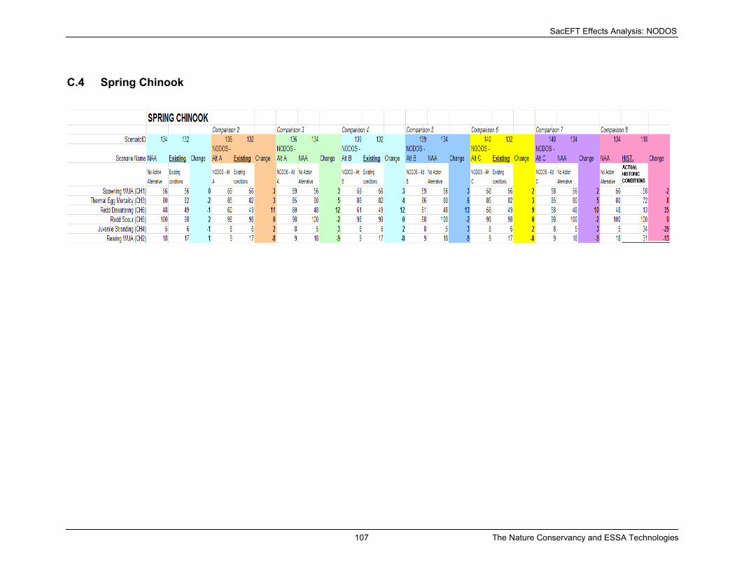
SacEFT Effects Analysis: NODOS
107 The Nature Conservancy and ESSA Technologies
C.4 Spring Chinook

SacEFT Effects Analysis: NODOS
108 The Nature Conservancy and ESSA Technologies

SacEFT Effects Analysis: NODOS
109 The Nature Conservancy and ESSA Technologies

SacEFT Effects Analysis: NODOS
110 The Nature Conservancy and ESSA Technologies

SacEFT Effects Analysis: NODOS
111 The Nature Conservancy and ESSA Technologies

SacEFT Effects Analysis: NODOS
112 The Nature Conservancy and ESSA Technologies

SacEFT Effects Analysis: NODOS
113 The Nature Conservancy and ESSA Technologies

SacEFT Effects Analysis: NODOS
114 The Nature Conservancy and ESSA Technologies
C.5 Winter Chinook

SacEFT Effects Analysis: NODOS
115 The Nature Conservancy and ESSA Technologies

SacEFT Effects Analysis: NODOS
116 The Nature Conservancy and ESSA Technologies

SacEFT Effects Analysis: NODOS
117 The Nature Conservancy and ESSA Technologies

SacEFT Effects Analysis: NODOS
118 The Nature Conservancy and ESSA Technologies

SacEFT Effects Analysis: NODOS
119 The Nature Conservancy and ESSA Technologies

SacEFT Effects Analysis: NODOS
120 The Nature Conservancy and ESSA Technologies

This page intentionally left blank.
Related Documents