Apparent-density mapping using entropic regularization

A

JH

©

GEOPHYSICS, VOL. 72, NO. 4 �JULY-AUGUST 2007�; P. I51–I60, 13 FIGS.10.1190/1.2732557

pparent-density mapping using entropic regularization

oão B. C. Silva1, Francisco S. Oliveira2, Valéria C. F. Barbosa3, andaroldo F. Campos Velho4

liputam

ml1gtaf2i

watrt1tmclwtt

t

t receive-mail: jr.Brazil.. E-mai

ABSTRACT

We present a new apparent-density mapping method onthe horizontal plane that combines the minimization of thefirst-order entropy with the maximization of the zeroth-orderentropy of the estimated density contrasts. The interpretationmodel consists of a grid of vertical, juxtaposed prisms in bothhorizontal directions. We assume that the top and the bottomof the gravity sources are flat and horizontal and estimate theprisms’density contrasts. The minimization of the first-orderentropy favors solutions presenting sharp borders, and themaximization of the zeroth-order entropy prevents the ten-dency of the source estimate to become a single prism. Thus,a judicious combination of both constraints may lead to solu-tions characterized by regions with virtually constant esti-mated density contrasts separated by sharp discontinuities.We apply our method to synthetic data from simulated intru-sive bodies in sediments that present flat and horizontal tops.By comparing our results with those obtained with thesmoothness constraint, we show that both methods producegood and equivalent locations of the sources’ central posi-tions. However, the entropic regularization delineates theboundaries of the bodies with greater resolution, even in thecase of 100-m-wide bodies separated by a distance as smallas 50 m. Both the proposed and the global smoothness con-straints are applied to real anomalies from the eastern Alpsand from the Matsitama intrusive complex, northeasternBotswana. In the first case, the entropic regularization delin-eates two sources, with a horizontal and nearly flat top beingconsistent with the known geologic information. In the sec-ond case, both constraints produce virtually the same esti-mate, indicating, in agreement with results of synthetic tests,that the tops of the sources are neither flat nor horizontal.

Manuscript received by the Editor November 14, 2006; revised manuscrip1Universidade Federal do Pará, Dep. Geofísica, CG, Belém, Pará, Brazil. E2Universidade Federal do Pará, Belém, Pará, Brazil. E-mail: [email protected]ório Nacional, Gal. José Cristino, São Cristóvão, Rio de Janeiro,4INPE, LAC,Av. dosAstronautas, São José dos Campos, São Paulo, Brazil2007 Society of Exploration Geophysicists.All rights reserved.

I51

INTRODUCTION

Geologic mapping is of the utmost importance in locating and de-ineating potential mineral targets. The production of a geologic mapncludes data collection in the field, aerial and satellite photo inter-retation, and geologic interpretation. Therefore, geologic mappingses information collected mainly at the earth’s surface. However,he elaboration of a reliable geologic model requires informationbout the structure and composition of deeper zones on the crust byeans of geophysical measurements �Maas et al., 2003�.The gravity method has been used as an auxiliary tool in geologicapping to locate and delineate both outcropping and buried geo-

ogic units and structures �Gupta and Grant, 1985; Granser et al.,989; Keating, 1992�. Gravity interpretation as an auxiliary tool foreologic mapping consists of estimating the spatial distribution ofhe density contrasts. This is not a trivial task because gravity datare not sufficient to estimate the distribution of density in the subsur-ace in a unique and stable way �Barbosa et al., 2002; Silva et al.,002�. Apparent-density mapping is therefore an ill-posed problemn the sense of Hadamard �1902�.

The most effective way to transform an ill-posed problem into aell-posed one is to incorporate a priori information about the

nomalous sources through optimizing a suitable stabilizing func-ional, subject to fitting the observations within the measurement er-ors by the computed anomaly produced by the estimated parame-ers of an assumed interpretation model �Tikhonov and Arsenin,977�. The choice of the particular functional to be optimized mustake into account the geologic setting; the geologic setting deter-

ines the geophysical inversion method to be used in the geophysi-al interpretation.As a result, whatever the method selected to stabi-ize the solution of the geophysical inverse problem, the solutionill be biased heavily toward the a priori information incorporated

hrough the selected functional, subject to the gravity data being fit-ed within measurement precision.

In the past, several authors developed different stabilizing func-ionals to locate and delineate geologic units and structures. To date,

d January 29, 2007; published online May 25, [email protected].

E-mail: [email protected]: [email protected].

mtltdaynz

�fiptsctilmmt

tcVtiwkttldbw

gfl

csvptn

feelmppbs

tdtpWti�

�ptm

wattit

pttaejp

s

wte�

z

Fmfl

I52 Silva et al.

ost geophysicists maximize the smoothness of the spatial distribu-ion of the physical property. In this procedure, the interpreter stabi-izes the solution at the expense of a decrease in the source delinea-ion resolution. Barbosa et al. �2002, Figure 2� estimate apparentensities by minimizing the Euclidean norm of the first-order deriv-tive of the density-contrast distribution along the x- and-directions. They assume the gravity sources have known thick-esses and depths to the top as well as vertical sides and flat and hori-ontal tops.

Ramos and Campos Velho �1996� and Campos Velho and Ramos1997� have developed a regularizing technique known as minimumrst-order entropy combined with the maximum zeroth-order entro-y of the estimated spatial distribution of the physical distribution;hey apply it to magnetotelluric data. This regularization method isubstantially different from classic regularization methods, whichonsist of maximizing the smoothness of the spatial distribution ofhe physical properties and its slightly modified versions. Minimiz-ng the first-order entropy leads to solutions presenting more abruptimits, in this way better delineating the contacts between the esti-

ated geologic units mapped by the proposed technique. The maxi-ization of the zeroth-order entropy prevents the tendency of the es-

imated source to become an equivalent point source.We present a new apparent-density mapping method using the en-

ropic regularization, defined by minimizing the first-order entropyombined with maximizing the zeroth-order entropy, as Camposelho and Ramos �1997� propose. We apply the method to estimate

he spatial distribution of the density contrast as a function of the hor-zontal coordinates only. We assume the sources are homogeneousith flat and horizontal tops and bottoms and that the interpreternows these depths beforehand. Minimization of the first-order en-ropy measure combined with maximization of the zeroth-order en-ropy measure restricts the solutions to a class of models comprisingocally homogeneous regions confined by sharp bounds and embed-ed in host rocks, which are also mainly homogeneous, allowing aetter delineation of the horizontal limits of the sources comparedith the method that incorporates the smoothness constraint.We apply the proposed method to synthetic data produced by two

roups of sources: those that satisfy the assumption of sources withat and horizontal tops and bottoms and those that do not. In the first

Elementary cell

Gravity sources

y

x

Observations

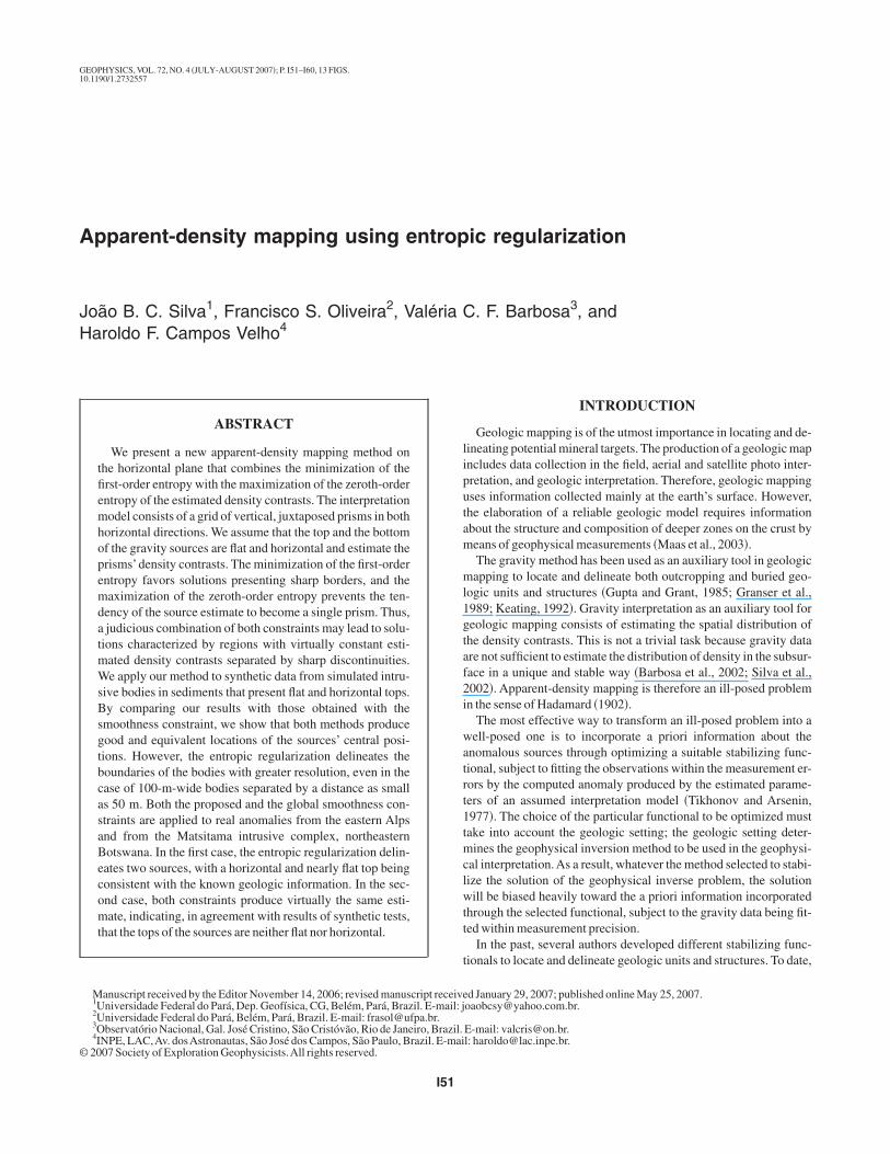
igure 1. Gravity sources, observations layout, and interpretationodel consisting of a set of rectangular, 3D juxtaposed prisms withat top and bottom.

ase, the estimated density-contrast distribution delineates theources with sharper borders and presents values closer to a constantalue over the presumably homogeneous anomalous sources com-ared with the smoothness constraint inversion. In the second case,he estimates produced by both methods are poor and present no sig-ificant difference.

We also apply the entropic regularization method to gravity datarom the eastern Alps and Matsitama �Botswana� regions. In theastern Alps, the entropic regularization produced density-contraststimates locally closer to constant values over the mapped anoma-ous sources, which is different from the smoothness constraint

ethod. This indicates that at least portions of the anomalous sourceresent approximately flat and horizontal tops and bottom and ap-roximately constant density contrast. Conversely, in Matsitama,oth methods present results very close to each other, indicating theource probably presents neither flat nor horizontal tops.

METHODOLOGY

Consider a set of homogeneous gravity sources. We assume thathe top and bottom of all sources are flat and horizontal and that theirepths are known �Figure 1�. We approximate these sources by an in-erpretation model consisting of a grid of 3D rectangular, juxtaposedrisms. We presume that the grid encloses all anomalous sources.e assume also that each prism has a constant density contrast and

hat the tops and bottoms of all prisms are at the same depth, coincid-ng, respectively, with the known tops and bottoms of the true sourceFigure 1�.

From a set of N gravity anomaly observations g0�p��g1

0, . . . ,gN0 �T, we estimate a vector p of density contrasts of each

rismatic cell of the interpretation model. If the information con-ained in the data were sufficient to estimate the parameters, we

ight obtain estimates of p by the minimization of

�g0 − g�p��2, �1�

here g�p� is an N-dimensional vector containing the computednomaly and � . � is the Euclidean norm. Obtaining the minimizers ofhe functional given in equation 1 is an ill-posed problem becausehe solution of this problem is unstable; therefore, it is necessary toncorporate additional a priori information about the sources toransform this problem into a well-posed one.

Traditionally, the a priori information incorporated in most geo-hysical inverse problems is the global smoothness of the spatial dis-ribution of the physical property, which consists of requiring thathe estimate of each parameter p̂i �density contrast of the ith cell� bes close as possible to the estimate of parameter p̂j �density-contraststimate of a neighboring cell either in the x- or the y-direction�, sub-ect to the observations being explained by the response of the inter-retation model. Mathematically, we have

minp

�pT RT Rp� , �2�

ubject to

�g0 − g�p��2 = � , �3�

here � is associated with the experimental error, T is the transposi-ion operator, and R is a matrix representing the first-order differ-nce operator, whose lines present just two nonnull elements �1 and1� at the columns associated with adjacent parameters p̂ and p̂ .

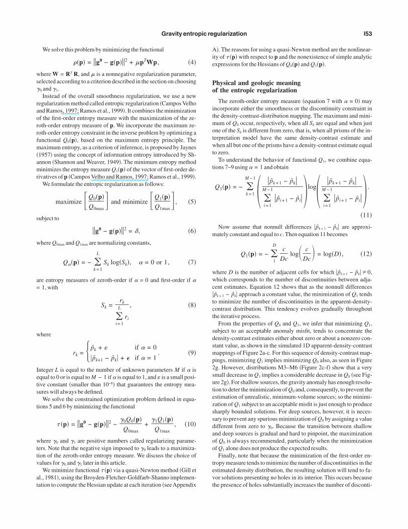
ws�

raorrfm�amr

s

w

a=

w

Iets

t

wttv

at

Aie

Po

itmotwt

t

m

wwc tct

sdsmp2sutezssdaoo

tevt

Gravity entropic regularization I53

We solve this problem by minimizing the functional

��p� = �g0 − g�p��2 + �pTWp , �4�

here W = RT R, and � is a nonnegative regularization parameter,elected according to a criterion described in the section on choosing0 and �1.Instead of the overall smoothness regularization, we use a new

egularization method called entropic regularization �Campos Velhond Ramos, 1997; Ramos et al., 1999�. It combines the minimizationf the first-order entropy measure with the maximization of the ze-oth-order entropy measure of p. We incorporate the maximum ze-oth-order entropy constraint in the inverse problem by optimizing aunctional Q0�p�, based on the maximum entropy principle. Theaximum entropy, as a criterion of inference, is proposed by Jaynes

1957� using the concept of information entropy introduced by Sh-nnon �Shannon and Weaver, 1949�. The minimum entropy methodinimizes the entropy measure Q1�p� of the vector of first-order de-

ivatives of p �Campos Velho and Ramos, 1997; Ramos et al., 1999�.We formulate the entropic regularization as follows:

maximize Q0�p�Q0max

and minimize Q1�p�Q1max

, �5�

ubject to

�g0 − g�p��2 = � , �6�

here Q0max and Q1max are normalizing constants,

Q��p� = − �k = 1

L

Sk log�Sk�, � = 0 or 1, �7�

re entropy measures of zeroth-order if � = 0 and first-order if �1, with

Sk =rk

�i = 1

L

ri

, �8�

here

rk = � p̂k + � if � = 0

p̂k+1 − p̂k + � if � = 1. �9�

nteger L is equal to the number of unknown parameters M if � isqual to 0 or is equal to M − 1 if � is equal to 1, and � is a small posi-ive constant �smaller than 10−8� that guarantees the entropy mea-ures will always be defined.

We solve the constrained optimization problem defined in equa-ions 5 and 6 by minimizing the functional

�p� = �g0 − g�p��2 −�0Q0�p�

Q0max+

�1Q1�p�Q1max

, �10�

here �0 and �1 are positive numbers called regularizing parame-ers. Note that the negative sign imposed to �0 leads to a maximiza-ion of the zeroth-order entropy measure. We discuss the choice ofalues for �0 and �1 later in this article.

We minimize functional �p� via a quasi-Newton method �Gill etl., 1981�, using the Broyden-Fletcher-Goldfarb-Shanno implemen-ation to compute the Hessian update at each iteration �seeAppendix

�. The reasons for using a quasi-Newton method are the nonlinear-ty of �p� with respect to p and the nonexistence of simple analyticxpressions for the Hessians of Q0�p� and Q1�p�.

hysical and geologic meaningf the entropic regularization

The zeroth-order entropy measure �equation 7 with � = 0� mayncorporate either the smoothness or the discontinuity constraint inhe density-contrast-distribution mapping. The maximum and mini-um of Q0 occur, respectively, when all Sk are equal and when just

ne of the Sk is different from zero, that is, when all prisms of the in-erpretation model have the same density-contrast estimate andhen all but one of the prisms have a density-contrast estimate equal

o zero.To understand the behavior of functional Q1, we combine equa-

ions 7–9 using � = 1 and obtain

Q1�p� = − �k = 1

M − 1

� p̂k + 1 − p̂k

�i = 1

M − 1

p̂i + 1 − p̂i �log� p̂k + 1 − p̂k

�i = 1

M − 1

p̂i + 1 − p̂i � .

�11�

Now assume that nonnull differences p̂k + 1 − p̂k are approxi-ately constant and equal to c. Then equation 11 becomes

Q1�p� = − �1

Dc

Dclog� c

Dc� = log�D� , �12�

here D is the number of adjacent cells for which p̂k + 1 − p̂k �0,hich corresponds to the number of discontinuities between adja-

ent estimates. Equation 12 shows that as the nonnull differencesp̂k + 1 − p̂k approach a constant value, the minimization of Q1 tendso minimize the number of discontinuities in the apparent-density-ontrast distribution. This tendency evolves gradually throughouthe iterative process.

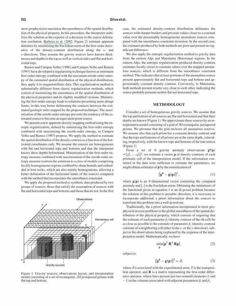
From the properties of Q0 and Q1, we infer that minimizing Q1,ubject to an acceptable anomaly misfit, tends to concentrate theensity-contrast estimates either about zero or about a nonzero con-tant value, as shown in the simulated 1D apparent-density-contrastappings of Figure 2a-c. For this sequence of density-contrast map-

ings, minimizing Q1 implies minimizing Q0 also, as seen in Figureg. However, distributions M3–M6 �Figure 2c-f� show that a verymall decrease in Q1 implies a considerable decrease in Q0 �see Fig-re 2g�. For shallow sources, the gravity anomaly has enough resolu-ion to deter the minimization of Q0 and, consequently, to prevent thestimation of unrealistic, minimum-volume sources; so the minimi-ation of Q1 subject to an acceptable misfit is just enough to produceharply bounded solutions. For deep sources, however, it is neces-ary to prevent any spurious minimization of Q0 by assigning a valueifferent from zero to �0. Because the transition between shallownd deep sources is gradual and hard to pinpoint, the maximizationf Q0 is always recommended, particularly when the minimizationf Q1 alone does not produce the expected results.

Finally, note that because the minimization of the first-order en-ropy measure tends to minimize the number of discontinuities in thestimated density distribution, the resulting solution will tend to fa-or solutions presenting no holes in its interior. This occurs becausehe presence of holes substantially increases the number of disconti-

nws

C

tirltotvfwa

pbw

otcdttttpcwtsm

S

mtddpWt

cTots

F�

Fiio

I54 Silva et al.

uities �and consequently the first-order entropy measure�. In thisay, the entropic regularization favors solutions displaying compact

ources.

hoice of parameters �0 and �1

We select parameters � �equation 4�, �0, and �1 �equation 10� inhe following way. Parameter � controls the solution stability, whichs obtained at the expense of a decrease in solution resolution. As aesult, it must be the smallest positive value still producing stable so-utions. Values of � larger than this optimum value increase the solu-ion smoothness beyond that necessary to produce a stable estimatef the sources limits, whereas smaller values produce unstable solu-ions. We characterize an unstable solution by perturbing the obser-ations with different sequences of pseudorandom noise realizationsor fixed value � and obtaining the corresponding solutions, whiche consider to be stable if they are sufficiently close to each other,

ccording to an established criterion.Conversely, �1 allows discontinuities in the solution �physical

roperties�. A small value of �1 produces a solution with undefinedorders in the same way that the global smoothness method does,hereas a large value of �1 produces solutions exhibiting spurious

a) 1.0

0.8

0.6

0.4

0.2

0.0

Horizontal distance (km) Den

sity

con

tras

t (g/

cm3 )

0 6 10

M1

15 20

b) 1.0

0.8

0.6

0.4

0.2

0.0

Horizontal distance (km) Den

sity

con

tras

t (g/

cm3 )

0 6 10

M2

15 20

c) 1.0

0.8

0.6

0.4

0.2

0.0

Horizontal distance (km) Den

sity

con

tras

t (g/

cm3 )

0 6 10

M3

15 20

d) 1.0

0.8

0.6

0.4

0.2

0.0

Horizontal distance (km) Den

sity

con

tras

t (g/

cm3 )

0 6 10

M4

15 20

e) 1.0

0.8

0.6

0.4

0.2

0.0

Horizontal distance (km) Den

sity

con

tras

t (g/

cm3 )

0 6 10

M5

15 20

f) 1.0

0.8

0.6

0.4

0.2

0.0

Horizontal distance (km) Den

sity

con

tras

t (g/

cm3 )

0 6 10

M6

15 20

g) 3

2

1

0

Apparent-density-contrast distribution

Ent

ropi

es Q

0 an

d Q

1

M1 M2

Q0

Q1

M3 M4 M5 M6

igure 2. One-dimensional density-contrast distributions M1–M6a–f� and the respective entropy measures of orders zero and one �g�.

scillations and discontinuities in the estimated density contrasts ofhe cells. These oscillations are not related to instability; rather, theyharacterize attempts to estimate sharp source limits. Their presenceemonstrates that we have overestimated the number of discontinui-ies in the physical property. In this way, �1 must be the largest posi-ive value leading to no more oscillations or discontinuities thanhose expected for the geologic body being interpreted. As shown inhe previous section, the entropy measures Q0 and Q1 are not inde-endent from each other, and the minimization of Q1 implies, underertain circumstances, the minimization of Q0, as well. As a result,e must assign provisionally to �0 a small value �including zero�. If

he solution collapses into a source whose horizontal dimensions areubstantially smaller than those expected for the true source, weust increase the value assigned to �0.

topping criterion

We interrupt the iterative process according to the followingathematical criterion. Consider the numerical values of the objec-

ive function �p� along the iterations �Figure 3�. A measure of theecay rate of �p� at the kth iteration is dk

�1� = �p̂k� − �p̂k−1�. Theecrease of this measure along successive iterations indicates theresence of a flat area in the behavior of �p� displayed in Figure 3.e detect the right-hand-side limit of this flat area by an increase in

he absolute value of dk�1�.

We interrupt the iterative process at the iteration k, where the firsthange of signal of dk

�2� �dk+1�1� − dk

�1� from positive to negative occurs.his mathematical criterion aims at stopping the iteration at the endf the first flat area of the behavior of function �p� along the itera-ion. We select the first flat area because the solutions associated withubsequent flat areas tend to produce smaller values of Q1�p� and,

5.5

5.0

4.5

4.0

3.5

3.0

Iteration

(p)

0 4 8 12

τ

16 20

igure 3. Schematic decay of the objective function �p� along theterations. The iterative process has been interrupted at the thirteenthteration �vertical arrow�, corresponding to the right-hand-side limitf the first flat area in the evaluation of �p�.

cpp

pbte

lxtd

atti

S

biaiwwtvt0pbs

sdnisFidwa5psw

tistl

wtsesmo

bseaorgdmt�

S

zvb

Gravity entropic regularization I55

onsequently, smaller values of Q0�p�. As a result, these solutionsresent more discontinuities or smaller sources than could be ex-ected for the geologic bodies we are interpreting.

APPLICATION TO SYNTHETIC DATA

In this section, we compare the solutions of the inverse gravityroblem as a function of the x- and y-variables using the classic glo-al smoothness method �minimizer of equation 4 with ��0� withhe solutions obtained with the entropic regularization �minimizer ofquation 10 with �1�0 and �0 = 0 or �0�0�.

The interpretation model consists of an nxny grid of rectangu-ar vertical prisms with dimensions dx and dy, juxtaposed along the- and y-directions, respectively. The synthetic models simulate in-rusive rocks in sediments or metasediments, presenting a constantensity contrast.

We present two tests with synthetic data, simulating the gravitynomaly produced by the intrusion of a granitic stock into sedimen-ary rocks. In the first test, the simulated source honors the conditionhat the source must have a flat and horizontal top; in the second test,t does not.

ource with flat top and flat bottom

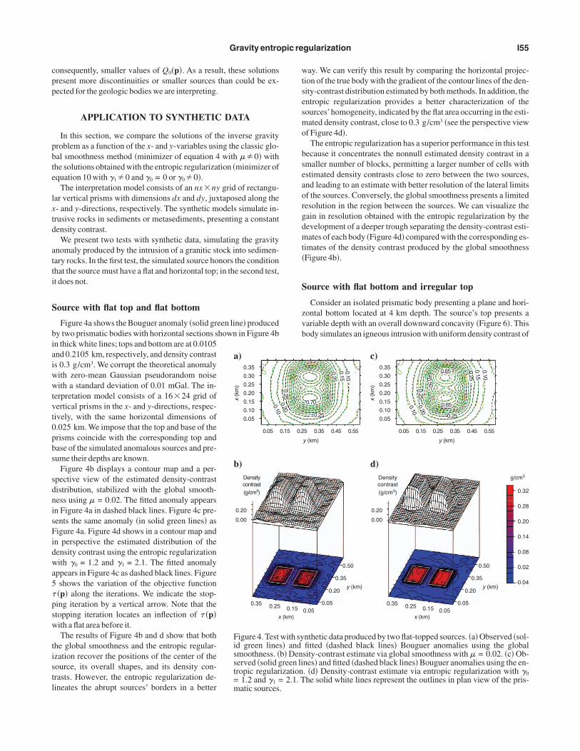
Figure 4a shows the Bouguer anomaly �solid green line� producedy two prismatic bodies with horizontal sections shown in Figure 4bn thick white lines; tops and bottom are at 0.0105nd 0.2105 km, respectively, and density contrasts 0.3 g/cm3. We corrupt the theoretical anomalyith zero-mean Gaussian pseudorandom noiseith a standard deviation of 0.01 mGal. The in-

erpretation model consists of a 1624 grid ofertical prisms in the x- and y-directions, respec-ively, with the same horizontal dimensions of.025 km. We impose that the top and base of therisms coincide with the corresponding top andase of the simulated anomalous sources and pre-ume their depths are known.

Figure 4b displays a contour map and a per-pective view of the estimated density-contrastistribution, stabilized with the global smooth-ess using � = 0.02. The fitted anomaly appearsn Figure 4a in dashed black lines. Figure 4c pre-ents the same anomaly �in solid green lines� asigure 4a. Figure 4d shows in a contour map and

n perspective the estimated distribution of theensity contrast using the entropic regularizationith �0 = 1.2 and �1 = 2.1. The fitted anomaly

ppears in Figure 4c as dashed black lines. Figureshows the variation of the objective function�p� along the iterations. We indicate the stop-ing iteration by a vertical arrow. Note that thetopping iteration locates an inflection of �p�ith a flat area before it.The results of Figure 4b and d show that both

he global smoothness and the entropic regular-zation recover the positions of the center of theource, its overall shapes, and its density con-rasts. However, the entropic regularization de-ineates the abrupt sources’ borders in a better

x (k

m)

a) 0.35

0.30

0.25

0.20

0.15

0.10

0.05

b)

0.20

0.00

0.25 0.35

0.05

Densitycontrast(g/cm3)

0.10

x

Figure 4. Testid green linesmoothness. �served �solid gtropic regular= 1.2 and �1 =matic sources

ay. We can verify this result by comparing the horizontal projec-ion of the true body with the gradient of the contour lines of the den-ity-contrast distribution estimated by both methods. In addition, thentropic regularization provides a better characterization of theources’homogeneity, indicated by the flat area occurring in the esti-ated density contrast, close to 0.3 g/cm3 �see the perspective view

f Figure 4d�.The entropic regularization has a superior performance in this test

ecause it concentrates the nonnull estimated density contrast in amaller number of blocks, permitting a larger number of cells withstimated density contrasts close to zero between the two sources,nd leading to an estimate with better resolution of the lateral limitsf the sources. Conversely, the global smoothness presents a limitedesolution in the region between the sources. We can visualize theain in resolution obtained with the entropic regularization by theevelopment of a deeper trough separating the density-contrast esti-ates of each body �Figure 4d� compared with the corresponding es-

imates of the density contrast produced by the global smoothnessFigure 4b�.

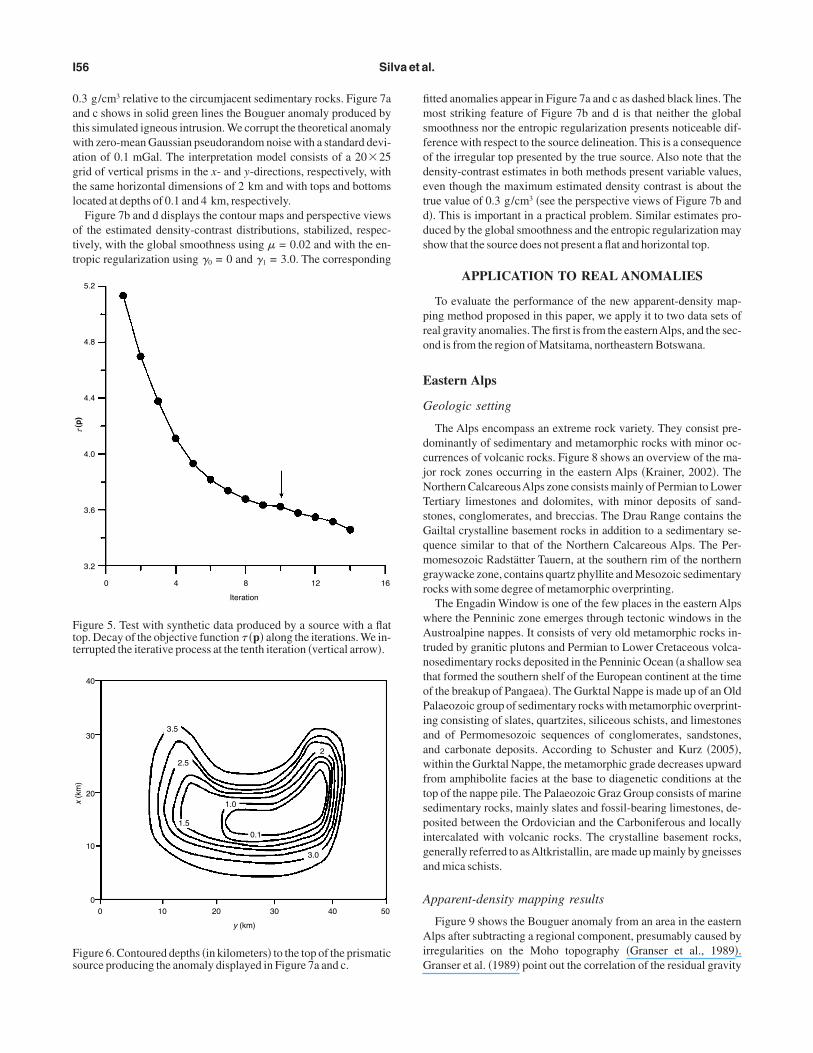
ource with flat bottom and irregular top

Consider an isolated prismatic body presenting a plane and hori-ontal bottom located at 4 km depth. The source’s top presents aariable depth with an overall downward concavity �Figure 6�. Thisody simulates an igneous intrusion with uniform density contrast of

y (km)

0.50

0.35

0.20

0.05 0.05

0.32

0.28

0.20

0.14

0.08

0.02

–0.04

g/cm3

5

0.25 0.25

0.70

0.65

0.65

0.250.20

0.50

0.10

0.100.15

0.25

0.100.150.25

0.35 0.45 0.55

y (km)

y (km)

d)

0.20

0.00

0.50

0.35

0.20

0.05 0.05 0.15 0.25 0.35

Densitycontrast(g/cm3)

x (km)

y (km)

x (k

m)

c) 0.35

0.30

0.25

0.20

0.15

0.10

0.05

0.05 0.15 0.25 0.35 0.45 0.55

nthetic data produced by two flat-topped sources. �a� Observed �sol-fitted �dashed black lines� Bouguer anomalies using the globalsity-contrast estimate via global smoothness with � = 0.02. �c� Ob-nes� and fitted �dashed black lines� Bouguer anomalies using the en-. �d� Density-contrast estimate via entropic regularization with �0

he solid white lines represent the outlines in plan view of the pris-

0.15

0.15 0.2

0.250.20

(km)

with sys� andb� Denreen li

ization2.1. T

.

0atwagtl

ott

fimsfodetdds

pro

E

G

dcjNTsGqmgr

wAtntoPiaawftspiga

A

AiG

Ftt

Fs

I56 Silva et al.

.3 g/cm3 relative to the circumjacent sedimentary rocks. Figure 7and c shows in solid green lines the Bouguer anomaly produced byhis simulated igneous intrusion. We corrupt the theoretical anomalyith zero-mean Gaussian pseudorandom noise with a standard devi-

tion of 0.1 mGal. The interpretation model consists of a 2025rid of vertical prisms in the x- and y-directions, respectively, withhe same horizontal dimensions of 2 km and with tops and bottomsocated at depths of 0.1 and 4 km, respectively.

Figure 7b and d displays the contour maps and perspective viewsf the estimated density-contrast distributions, stabilized, respec-ively, with the global smoothness using � = 0.02 and with the en-ropic regularization using �0 = 0 and �1 = 3.0. The corresponding

5.2

4.8

4.4

4.0

3.6

3.2

Iteration

(p)

0 4 8 12

τ

16

igure 5. Test with synthetic data produced by a source with a flatop. Decay of the objective function �p� along the iterations. We in-errupted the iterative process at the tenth iteration �vertical arrow�.

40

30

20

10

0

y (km)

x (k

m)

0 10

3.5

2.5

1.5

1.0

0.1

2

3.0

20 30 40 50

igure 6. Contoured depths �in kilometers� to the top of the prismaticource producing the anomaly displayed in Figure 7a and c.

tted anomalies appear in Figure 7a and c as dashed black lines. Theost striking feature of Figure 7b and d is that neither the global

moothness nor the entropic regularization presents noticeable dif-erence with respect to the source delineation. This is a consequencef the irregular top presented by the true source. Also note that theensity-contrast estimates in both methods present variable values,ven though the maximum estimated density contrast is about therue value of 0.3 g/cm3 �see the perspective views of Figure 7b and�. This is important in a practical problem. Similar estimates pro-uced by the global smoothness and the entropic regularization mayhow that the source does not present a flat and horizontal top.

APPLICATION TO REAL ANOMALIES

To evaluate the performance of the new apparent-density map-ing method proposed in this paper, we apply it to two data sets ofeal gravity anomalies. The first is from the easternAlps, and the sec-nd is from the region of Matsitama, northeastern Botswana.

astern Alps

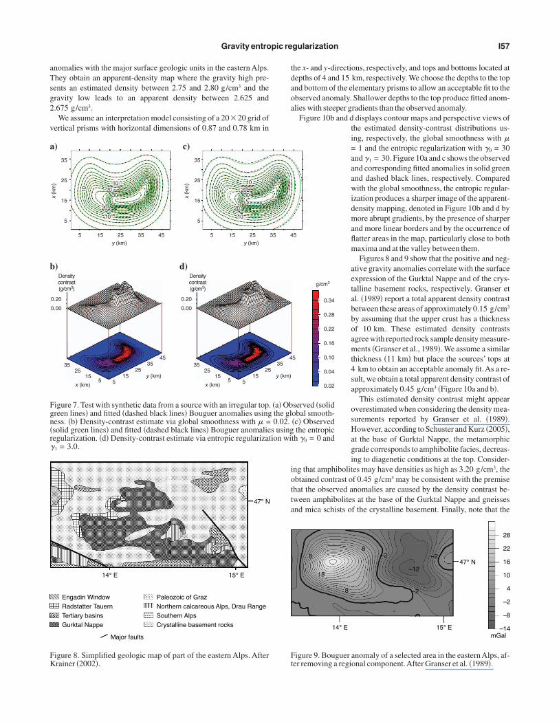
eologic setting

The Alps encompass an extreme rock variety. They consist pre-ominantly of sedimentary and metamorphic rocks with minor oc-urrences of volcanic rocks. Figure 8 shows an overview of the ma-or rock zones occurring in the eastern Alps �Krainer, 2002�. Theorthern CalcareousAlps zone consists mainly of Permian to Lowerertiary limestones and dolomites, with minor deposits of sand-tones, conglomerates, and breccias. The Drau Range contains theailtal crystalline basement rocks in addition to a sedimentary se-uence similar to that of the Northern Calcareous Alps. The Per-omesozoic Radstätter Tauern, at the southern rim of the northern

raywacke zone, contains quartz phyllite and Mesozoic sedimentaryocks with some degree of metamorphic overprinting.

The Engadin Window is one of the few places in the eastern Alpshere the Penninic zone emerges through tectonic windows in theustroalpine nappes. It consists of very old metamorphic rocks in-

ruded by granitic plutons and Permian to Lower Cretaceous volca-osedimentary rocks deposited in the Penninic Ocean �a shallow seahat formed the southern shelf of the European continent at the timef the breakup of Pangaea�. The Gurktal Nappe is made up of an Oldalaeozoic group of sedimentary rocks with metamorphic overprint-

ng consisting of slates, quartzites, siliceous schists, and limestonesnd of Permomesozoic sequences of conglomerates, sandstones,nd carbonate deposits. According to Schuster and Kurz �2005�,ithin the Gurktal Nappe, the metamorphic grade decreases upward

rom amphibolite facies at the base to diagenetic conditions at theop of the nappe pile. The Palaeozoic Graz Group consists of marineedimentary rocks, mainly slates and fossil-bearing limestones, de-osited between the Ordovician and the Carboniferous and locallyntercalated with volcanic rocks. The crystalline basement rocks,enerally referred to asAltkristallin, are made up mainly by gneissesnd mica schists.

pparent-density mapping results

Figure 9 shows the Bouguer anomaly from an area in the easternlps after subtracting a regional component, presumably caused by

rregularities on the Moho topography �Granser et al., 1989�.ranser et al. �1989� point out the correlation of the residual gravity

aTsg2

v

tdaoa

iotta

a

b

Fgn�r�

FK

Ft

Gravity entropic regularization I57

nomalies with the major surface geologic units in the eastern Alps.hey obtain an apparent-density map where the gravity high pre-ents an estimated density between 2.75 and 2.80 g/cm3 and theravity low leads to an apparent density between 2.625 and.675 g/cm3.

We assume an interpretation model consisting of a 2020 grid ofertical prisms with horizontal dimensions of 0.87 and 0.78 km in

y (km)

x (k

m)

)35

25

15

5

)

0.20

0.00

453535

25251515

55

5

10

10

10 20

20

30

15 25 35 45y (km)

x (k

m)

c)35

25

15

5

5

10

1010 20

20

30

15 25

Densitycontrast(g/cm3)

x (km)

y (km)

d)

0.20

0.00

352525

151555

Densitycontrast(g/cm3)

x (km)

igure 7. Test with synthetic data from a source with an irregular topreen lines� and fitted �dashed black lines� Bouguer anomalies usingess. �b� Density-contrast estimate via global smoothness with � =solid green lines� and fitted �dashed black lines� Bouguer anomalieegularization. �d� Density-contrast estimate via entropic regularizat1 = 3.0.

Engadin WindowRadstatter TauernTertiary basinsGurktal Nappe

Paleozoic of Graz Northern calcareous Alps, Drau Range Southern Alps Crystalline basement rocks

47° N

15° E

Major faults

14° E

igure 8. Simplified geologic map of part of the eastern Alps. Afterrainer �2002�.

he x- and y-directions, respectively, and tops and bottoms located atepths of 4 and 15 km, respectively. We choose the depths to the topnd bottom of the elementary prisms to allow an acceptable fit to thebserved anomaly. Shallower depths to the top produce fitted anom-lies with steeper gradients than the observed anomaly.

Figure 10b and d displays contour maps and perspective views ofthe estimated density-contrast distributions us-ing, respectively, the global smoothness with �= 1 and the entropic regularization with �0 = 30and �1 = 30. Figure 10a and c shows the observedand corresponding fitted anomalies in solid greenand dashed black lines, respectively. Comparedwith the global smoothness, the entropic regular-ization produces a sharper image of the apparent-density mapping, denoted in Figure 10b and d bymore abrupt gradients, by the presence of sharperand more linear borders and by the occurrence offlatter areas in the map, particularly close to bothmaxima and at the valley between them.

Figures 8 and 9 show that the positive and neg-ative gravity anomalies correlate with the surfaceexpression of the Gurktal Nappe and of the crys-talline basement rocks, respectively. Granser etal. �1989� report a total apparent density contrastbetween these areas of approximately 0.15 g/cm3

by assuming that the upper crust has a thicknessof 10 km. These estimated density contrastsagree with reported rock sample density measure-ments �Granser et al., 1989�. We assume a similarthickness �11 km� but place the sources’ tops at4 km to obtain an acceptable anomaly fit. As a re-sult, we obtain a total apparent density contrast ofapproximately 0.45 g/cm3 �Figure 10a and b�.

This estimated density contrast might appearoverestimated when considering the density mea-surements reported by Granser et al. �1989�.However, according to Schuster and Kurz �2005�,at the base of Gurktal Nappe, the metamorphicgrade corresponds to amphibolite facies, decreas-ing to diagenetic conditions at the top. Consider-

ng that amphibolites may have densities as high as 3.20 g/cm3, thebtained contrast of 0.45 g/cm3 may be consistent with the premisehat the observed anomalies are caused by the density contrast be-ween amphibolites at the base of the Gurktal Nappe and gneissesnd mica schists of the crystalline basement. Finally, note that the

0.34

0.28

0.22

0.16

0.10

0.04

0.02

5

g/cm3

5

served �solidobal smooth-�c� Observedthe entropic

th �0 = 0 and

28

22

16

10

4

–2

–8

–14mGal

47° N

15° E14° E

18

88

8

–2 –2

–2

–12

igure 9. Bouguer anomaly of a selected area in the eastern Alps, af-er removing a regional component.After Granser et al. �1989�.

35 4

435

y (km)

. �a� Obthe gl0.02.

s usingion wi

aMtaspb

A

gstbsitdi

pzd

tgwssc

FBsBe 0 1

FB�i

FFd

I58 Silva et al.

negative anomaly, which correlates with the crys-talline rocks, leads to a flat-bottom valley in thedensity-contrast map �Figure 10d�, whereas thepositive anomaly, correlated with the GurktalNappe, leads to a hill with more irregular top, pre-senting, just locally, areas with flat tops. This dif-ference may be related to the greater variety ofrocks and structures in the Gurktal Nappe com-pared with the crystalline rocks.

Matsitama igneous complex, Botswana

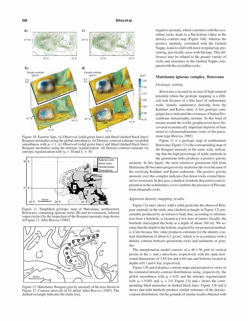
Geologic setting

Botswana is located in an area of high mineralpotential where the geologic mapping is a diffi-cult task because of a thin layer of sedimentaryrocks �mainly sandstones� deriving from theKalahari and Karoo units. A few geologic cam-paigns have indicated the existence of buried Pre-cambrian metamorphic terrains. In this kind ofterrain around the world, geophysicists have dis-covered economically important deposits of basemetal in volcanosedimentary rocks of the green-stone type �Reeves, 1985�.

Figure 11 is a geologic map of northeasternBotswana; Figure 12 is the corresponding map ofthe Bouguer anomaly in the same scale, indicat-ing that the high percentage of mafic minerals inthe greenstone belts produces a positive gravity

nomaly. In this figure, the most extensive greenstone belt fromatsitama �B� becomes progressively masked to the west because of

he overlying Kalahari and Karoo sediments. The positive gravitynomaly over this complex indicates that dense rocks extend them-elves westward. In this area, a shallow borehole directed to coal ex-loration in the sedimentary cover confirms the presence of Precam-rian ultramafic rocks.

pparent-density mapping results

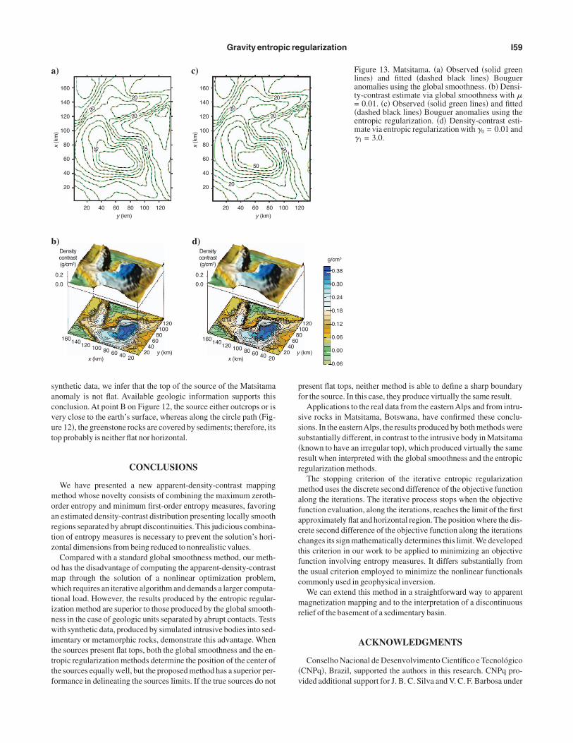
Figure 13a and c shows with a solid green line the observed Bou-uer anomaly in the study area �dashed rectangle in Figure 12� pre-umably produced by an intrusive body that, according to informa-ion from a borehole, is located at a few tens of meters �locally, theorehole intercepted the body at a depth of about 100 m�. We as-ume that the depth to the bottom, required by our proposed method,s 4 km because this value produces estimates for the density-con-rast distribution of about 0.3 g/cm3, which is in accordance with aensity contrast between greenstone rocks and sediments or gran-tes.

The interpretation model consists of a 4636 grid of verticalrisms in the x- and y-directions, respectively with the same hori-ontal dimensions of 3.85 km and with tops and bottoms located atepths of 0.1 and 4 km, respectively.

Figure 13b and d displays contour maps and perspective views ofhe estimated density-contrast distributions using, respectively, thelobal smoothness with � = 0.01 and the entropic regularizationith �0 = 0.001 and �1 = 3.0. Figure 13a and c shows the corre-

ponding fitted anomalies in dashed black lines. Figure 13b and dhows that both methods produce similar estimates of the density-ontrast distribution. On the grounds of similar results obtained with

0.32

0.24

0.16

0.08

0.00

–0.08

–0.16

5° E

5° E

g/cm3

black lines�ate via global

black lines�estimate via

a)

b)

0.2 0.0

47° N

47° N

14° E

2614

14

2

2

2

10

–10

15° E

14° E

15° E0.12

0.120.12

0.12

0.2

0.04

0.04 –0

.04

–0.0

40

0

0

0 0

c)

47° N

14° E

2614

14

2

2

2

10

–10

1

Density contrast(g/cm3)

d)

0.2 0.0

47° N

14° E

1

Density contrast(g/cm3)

igure 10. Eastern Alps. �a� Observed �solid green lines� and fitted �dashedouguer anomalies using the global smoothness. �b� Density-contrast estim

moothness with � = 1. �c� Observed �solid green lines� and fitted �dashedouguer anomalies using the entropic regularization. �d� Density-contrastntropic regularization with � = 30 and � = 30.

B

50 km25° E 26° E 27° E

21° S

20° SKalahari cover

Karoo cover

Granite-gneiss

Greenstones

igure 11. Simplified geologic map of Matsitama, northeasternotswana, containing igneous rocks �B� and its extension, inferred

open circles� by the inspection of the Bouguer anomaly map shownn Figure 12.After Reeves �1985�.

–100

–100

–90

–100

–100

–100

50 km

–110

–110

–110

–110

–120

–90

–90

–90–90

–80–70

B

–120

–120

igure 12. Matsitama. Bouguer gravity anomaly of the area shown inigure 11. Contour intervals of 10 mGal. After Reeves �1985�. Theashed rectangle indicates the study area.

sacvut

moartz

omwtinwitttf

pf

sss�rr

mafacctftc

mr

�v

a

b

Gravity entropic regularization I59

ynthetic data, we infer that the top of the source of the Matsitamanomaly is not flat. Available geologic information supports thisonclusion. At point B on Figure 12, the source either outcrops or isery close to the earth’s surface, whereas along the circle path �Fig-re 12�, the greenstone rocks are covered by sediments; therefore, itsop probably is neither flat nor horizontal.

CONCLUSIONS

We have presented a new apparent-density-contrast mappingethod whose novelty consists of combining the maximum zeroth-

rder entropy and minimum first-order entropy measures, favoringn estimated density-contrast distribution presenting locally smoothegions separated by abrupt discontinuities. This judicious combina-ion of entropy measures is necessary to prevent the solution’s hori-ontal dimensions from being reduced to nonrealistic values.

Compared with a standard global smoothness method, our meth-d has the disadvantage of computing the apparent-density-contrastap through the solution of a nonlinear optimization problem,hich requires an iterative algorithm and demands a larger computa-

ional load. However, the results produced by the entropic regular-zation method are superior to those produced by the global smooth-ess in the case of geologic units separated by abrupt contacts. Testsith synthetic data, produced by simulated intrusive bodies into sed-

mentary or metamorphic rocks, demonstrate this advantage. Whenhe sources present flat tops, both the global smoothness and the en-ropic regularization methods determine the position of the center ofhe sources equally well, but the proposed method has a superior per-ormance in delineating the sources limits. If the true sources do not

y (km)

x (k

m)

)

160

140

120

100

80

60

40

20

)

0.2

0.0

120

120140160

100

100

80

0.14

0.14

0.14

0.24

0.04

0.16

80

60

6040

40 2020

120140160

100 80 60 40 20

20 40 60 80 100 120

45

20

20

20

20

y (km)

x (k

m)

c)

160

140

120

100

80

60

40

20

20 40 60 80

20

2

20

50

20

Densitycontrast(g/cm3)

x (km)y (km)

d)

0.2

0.0

0.14

0.14

0.2

0.24

0.04 0.04

Densitycontrast(g/cm3)

x (km)

resent flat tops, neither method is able to define a sharp boundaryor the source. In this case, they produce virtually the same result.

Applications to the real data from the easternAlps and from intru-ive rocks in Matsitama, Botswana, have confirmed these conclu-ions. In the easternAlps, the results produced by both methods wereubstantially different, in contrast to the intrusive body in Matsitamaknown to have an irregular top�, which produced virtually the sameesult when interpreted with the global smoothness and the entropicegularization methods.

The stopping criterion of the iterative entropic regularizationethod uses the discrete second difference of the objective function

long the iterations. The iterative process stops when the objectiveunction evaluation, along the iterations, reaches the limit of the firstpproximately flat and horizontal region. The position where the dis-rete second difference of the objective function along the iterationshanges its sign mathematically determines this limit. We developedhis criterion in our work to be applied to minimizing an objectiveunction involving entropy measures. It differs substantially fromhe usual criterion employed to minimize the nonlinear functionalsommonly used in geophysical inversion.

We can extend this method in a straightforward way to apparentagnetization mapping and to the interpretation of a discontinuous

elief of the basement of a sedimentary basin.

ACKNOWLEDGMENTS

Conselho Nacional de Desenvolvimento Científico e TecnológicoCNPq�, Brazil, supported the authors in this research. CNPq pro-ided additional support for J. B. C. Silva and V. C. F. Barbosa under

0.38

0.30

0.24

0.18

0.12

0.06

0.00

–0.06

0

g/cm3

1201000

(km)

Figure 13. Matsitama. �a� Observed �solid greenlines� and fitted �dashed black lines� Bougueranomalies using the global smoothness. �b� Densi-ty-contrast estimate via global smoothness with �= 0.01. �c� Observed �solid green lines� and fitted�dashed black lines� Bouguer anomalies using theentropic regularization. �d� Density-contrast esti-mate via entropic regularization with �0 = 0.01 and�1 = 3.0.

100 12

0

20

8

0.14

4

6040

20 y

cF4Hvofi

Gtt

1

2

3

d

wHe

45

6

s

B

C

G

G

G

H

J

K

K

M

M

R

R

R

S

S

S

T

I60 Silva et al.

ontracts 504419/2004-8, 505265/2004-4, and 471168/2004-1.APERJ �contract E-26/170.733/2004� and CNPq �contract74878/2006-6� supported V. C. F. Barbosa, and FAPESP supported. F. Campos Velho. We thank Steven Arcone, Xiong Li, and re-iewers Pierre Keating and Olivier Boulanger for helpful commentsn this manuscript. We greatly appreciate constructive and thought-ul comments of Colin Farquharson. We thank Chrysa Cullather formproving the readability.

APPENDIX A

QUASI-NEWTON OPTIMIZATION ALGORITHMBY UPDATING THE HESSIAN MATRIX VIA THE

BROYDEN-FLETCHER-GOLDFARB-SHANNOMETHOD

We used the quasi-Newton method with the Broyden-Fletcher-oldfarb-Shanno implementation to minimize the objective func-

ion �p� given by equation 10. At the kth iteration, the quasi-New-on algorithm consists of the following steps:

� Solve the direct problem for p̂k and compute the objective func-tion �p̂k�.

� Compute by finite differences the M-dimensional gradient vec-tor �p� �p�� p = p̂k

of the function �p� with respect to vector p,evaluated at p = p̂k.

� Estimate the step �p̂k by solving the linear equation

Hk�p̂k = − �p� �p�� p = p̂k, �A-1�

where Hk is the quasi-Newton approximation to the M MHessian matrix of the function �p�.

The linear equationA-1 is obtained by minimizing the second-or-er functional given by

���pk� = �pT� �p�� p = p̂k

�pk +1

2�pk

THk�pk

ith respect to the search direction vector �pk. To guarantee theessian matrix is positive-definite, we use Marquardt’s �1963� strat-

gy at each iteration. Then we continue the steps.

� Obtain p̂k + 1 = p̂k + �p̂k.� Update the Hessian matrix using the Broyden-Fletcher-Gold-

farb-Shanno implementation by

Hk+1 = Hk +bkbk

T

bkTuk

−Hk�ukuk

T�Hk

ukTHkuk

, �A-2�

where bk = p̂k + 1 − p̂k and uk = �p� �p�� p = p̂k+1

− �p� �p�� p = p̂k.

� Test for algorithm convergence following the stopping criteri-on described in the “Methodology” section. If convergence isachieved, the iteration is stopped; otherwise increment k and goto step 1.

We initialize the iteration by making p̂o equal to the globalmoothness solution and H0 equal to the identity matrix I.

REFERENCES

arbosa, V. C. F., J. B. C. Silva, and W. E. Medeiros, 2002, Practical applica-tions of uniqueness theorems in gravimetry: Part II — Pragmatic incorpo-ration of concrete geologic information: Geophysics, 67, 795–800.

ampos Velho, H. F., and F. M. Ramos, 1997, Numerical inversion of two-dimensional geoelectric conductivity distributions from electromagneticground data: Revista Brasileira de Geofísica, 15, 133–144.

ill, P. E., W. Murray, and M. H. Wright, 1981, Practical optimization: Aca-demic Press Inc.

ranser, H., B. Meurers, and P. Steinhauser, 1989, Apparent density map-ping and 3D gravity inversion in the eastern Alps: Geophysical Prospect-ing, 37, 279–292.

upta, V. K., and F. S. Grant, 1985, Mineral-exploration aspects of gravityand aeromagnetic surveys in the Sudbury-Cobalt area, Ontario, in W. J.Hinze, ed. The utility of regional gravity and magnetic anomaly maps:SEG, 393–412.

adamard, J., 1902, Sur les problèmes aux dérivées partielles et leur signifi-cation physique: Bulletin of Princeton University, 13, 1–20.

aynes, E. T., 1957, Information theory and statistical mechanics: PhysicalReview, 106, 620–630.

eating, P., 1992, Density mapping from gravity data using the Walsh trans-form: Geophysics, 57, 637–642.

rainer, K., 2002, The Alps — Structural history of a mountain chain, in I.Ackerl, ed. The wonderful world of mountains: TheAustrianAlps: FederalPress Service, 10–22.aas, M. V. R., C. G. Oliveira, A. C. B. Pires, and R. A. V. Moraes, 2003, Air-borne geophysics applied to mineral exploration and geologic mapping inthe southwest sector of Orós-Jaguaribe copper belt, northeastern Brazil:Revista Brasileira de Geociências �in Portuguese�, 33, 279–288.arquardt, D. W., 1963, An algorithm for least-squares estimation of nonlin-ear parameters: Journal of the Society of Industrial and Applied Mathe-matics, 2, 601–612.

amos, F. M., and H. F. Campos Velho, 1996, Reconstruction of geoelectricconductivity distributions using a minimum first-order entropy technique:2nd International Conference on Inverse Problems on Engineering, Pro-ceedings, 199–206.

amos, F. M., H. F. Campos Velho, J. C. Carvalho, and N. J. Ferreira, 1999,Novel approaches on entropic regularization: Inverse Problems, 15, 1139–1148.

eeves, C. V., 1985, The Kalahari Desert, central southernAfrica:Acase his-tory of regional gravity and magnetic exploration, in W. J. Hinze, eds., Theutility of regional gravity and magnetic anomaly maps: SEG, 144–153.

chuster, R., and W. Kurz, 2005, Eclogites in the eastern alps: High-pressuremetamorphism in the context of the alpine orogeny: Mitteilungsblatt derÖsterreichische Mineralogische Gesellschaft, 150, 173–188.

hannon, C. E., and W. Weaver, 1949, The mathematical theory of communi-cation: University. of Illinois Press.

ilva, J. B. C., W. E. Medeiros, and V. C. F. Barbosa, 2002, Practical applica-tions of uniqueness theorems in gravimetry: Part I — Constructing soundinterpretation methods: Geophysics, 67, 788–794.

ikhonov, A. N., and V. Y. Arsenin, 1977, Solutions of ill-posed problems: V.H. Winston & Sons.