APEX Septum Analysis G.M. Urciuoli. Comparison between PREX septum field (from SNAKE input), and APEX septum field (from TOSCA simulations). Y axis.

APEX Septum Analysis

G.M. Urciuoli

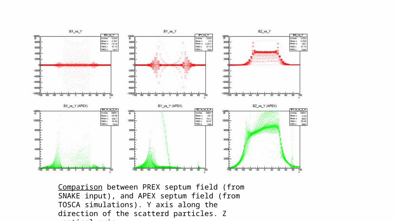
Comparison between PREX septum field (from SNAKE input), and APEX septum field (from TOSCA simulations). Y axis along the direction of the scatterd particles. Z vertical axis.

OPTIC performances

Optic simulations performed mainly through SNAKE.

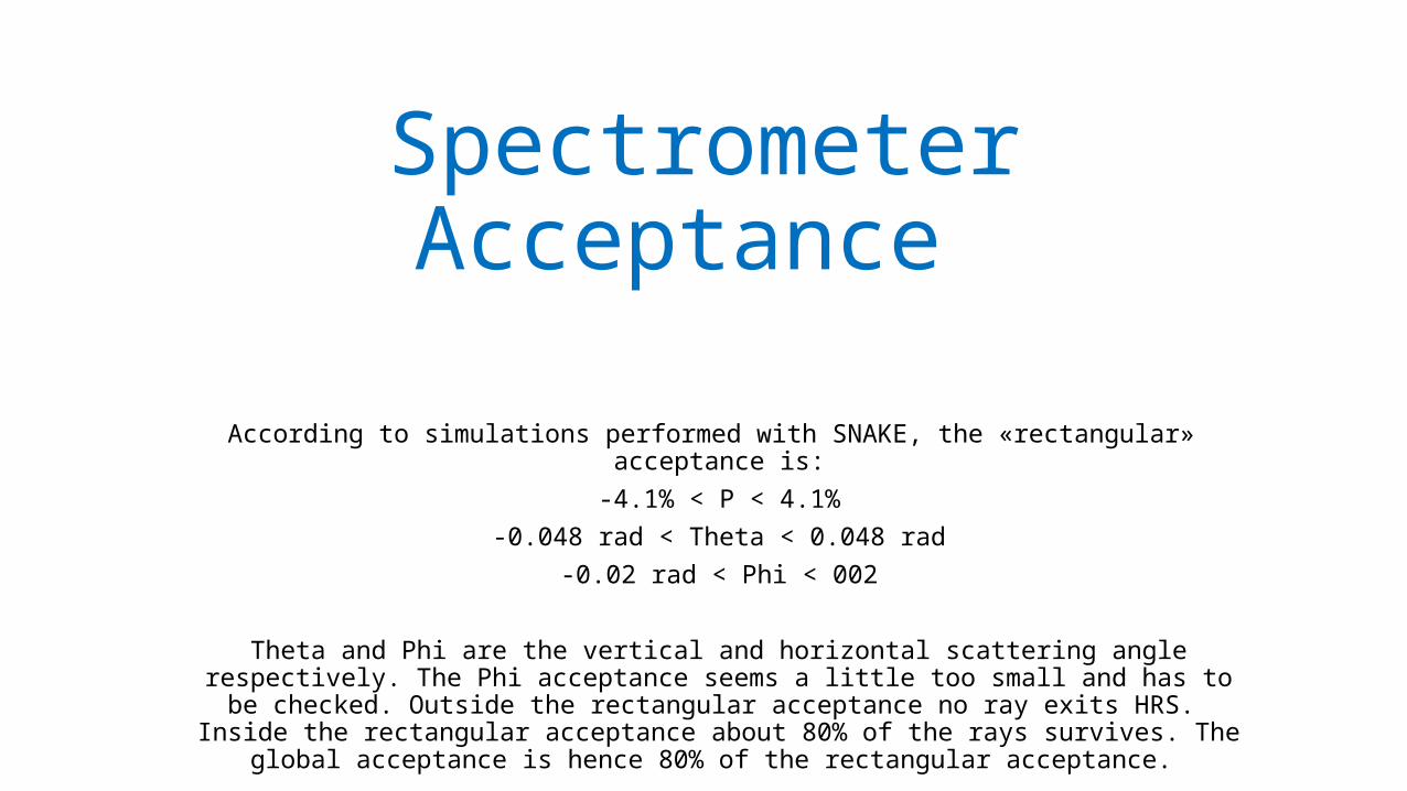
Spectrometer Acceptance

According to simulations performed with SNAKE, the «rectangular» acceptance is:-4.1% < P < 4.1%

-0.048 rad < Theta < 0.048 rad-0.02 rad < Phi < 002

Theta and Phi are the vertical and horizontal scattering angle respectively. The Phi acceptance seems a little too small and has to be checked. Outside the rectangular

acceptance no ray exits HRS. Inside the rectangular acceptance about 80% of the rays survives. The global acceptance is hence 80% of the rectangular acceptance.

Focal Plane at VDC• APEX septum is very close to the septum used by PREX. However PREX run with

a focal plane located 1.403 m downstream with respect to the VDCs. To find the correct HRS quadrupole setting that places the focal plane at VDC position one has to change HRS quadrupole fields (mainly Q3 one) in order to change the focal plane position with respet to PREX. The focal plane is at VDC position when the X spot size, produced by rays at the centre of the HRS momentum and horizontal angle acceptance, but spanning all over the vertical (Theta) scattering angle acceptance has its minimum at VDC position. This because, at focus, X is independent of Theta scattering angle.

• To place the focal plane at VDC position one has to reduce the Q3 field with respect to PREX setting of 13% (at the same momentum setting).

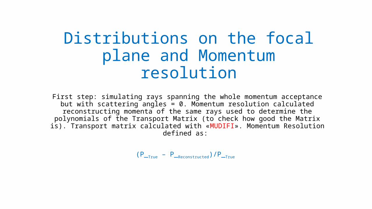
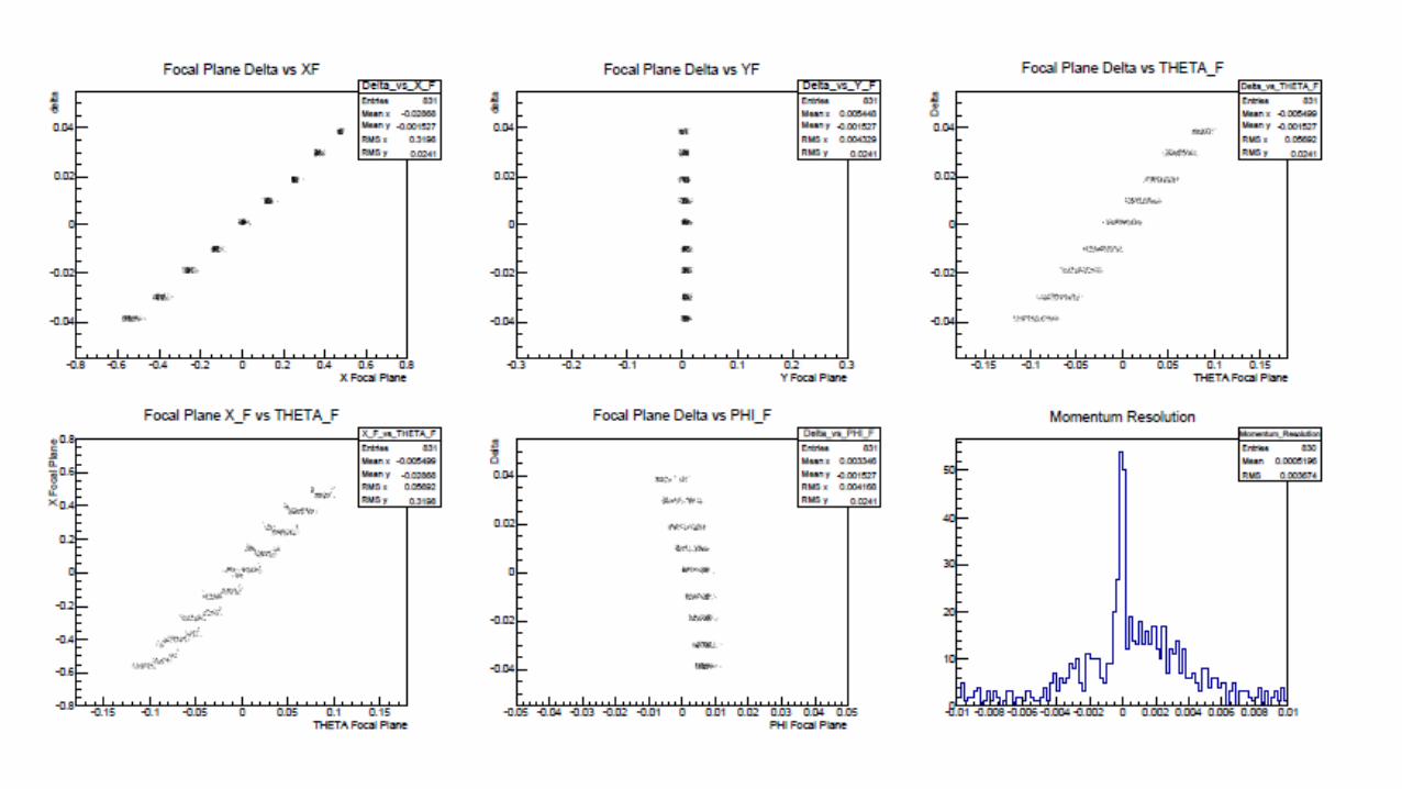
Distributions on the focal plane and Momentum resolution

First step: simulating rays spanning the whole momentum acceptance but with scattering angles = 0. Momentum resolution calculated reconstructing momenta of the same rays used to determine the polynomials of the Transport Matrix (to check how good the Matrix is). Transport matrix calculated with «MUDIFI». Momentum

Resolution defined as:

(P_True – P_Reconstructed)/P_True

Second step

• 1000 rays randomly chosen in the momentum range but with scattering angles still equal to zero. Their momenta reconstructed through the Transport Matrix deduced in indipendent way with MUDIFI during the previous step. During the reconstruction process, the ray coordinates on the focal plane were broadened according gaussian distributions. The sigmas of these gaussian distributions of the coordinates in the focal plane were: • σx = 2.3*10-4 m• σy = 2.5*10-4 m• σϑ = 2.95*10-4 rad• σϕ = 4.0*10-4 rad

Third Step

• Spanned all the momentum and vertical (theta) angle to derive a new Transport Matrix. The Matrix was used to trace back the same rays employed to derive it (see Momentum Resolution plot in next slide). The ray coordinates on the focal plane broadened according gaussian distributions• Now the resolution is worsend by the fact that XFocal Plane and ThetaFocal

Plane are extremely correlated and the simultaneous use of both of them in the determination (throug MUDIFI) of the Transport Matrix without elminating their correlation (not yet performed) can even worsen things. Netherteless the Momentum resolution is still very good.

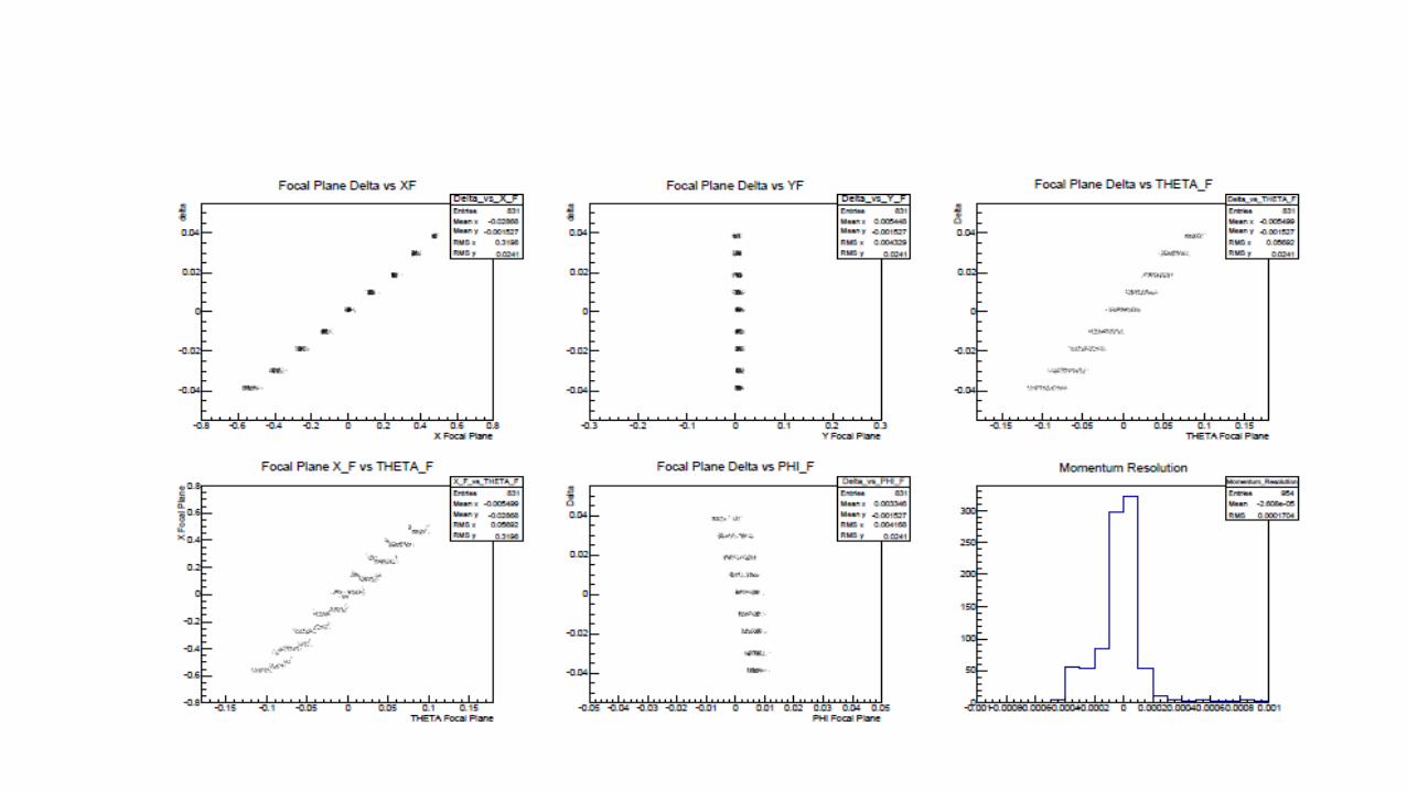
Fourth Step

1000 rays random chosen in the momentum range and vertical range. Their momenta reconstructed through the Transport Matrix deduced in indipendent way with MUDIFI during the previous step. The ray coordinates on the focal plane broadened according gaussian distributions (with respect to the corresponding plot of the third step, the momentum resolution plot has a different binning). The resolution still well less than 5*10-4.

To be done

• For momentum resolution: optical simulations that span rays also in the horizontal angle scattering acceptance.• Check on horizontal angle acceptance.• Simulations that take into accounts the target length.• Simulations that take into accounts the fact that the incident beam is

rastered. • Scattering angle resolution estimation.• Vertex reconstruction.• Target straggling etc. effects

Conclusions

The analysis has not yet be completed. Nevertheless APEX septum features seem to be pretty good. HRS outstanding performances (above all it momentum resolution) seem not to be spoiled by the introduction of the septum.