Apex Point Map for Constant-Time Bounding Plane Approximation Samuli Laine Tero Karras NVIDIA.

Apex Point Map for Constant-Time Bounding Plane Approximation

Samuli Laine

Tero Karras

NVIDIA

The Problem

How to quickly find a good bounding plane with a given orientation?

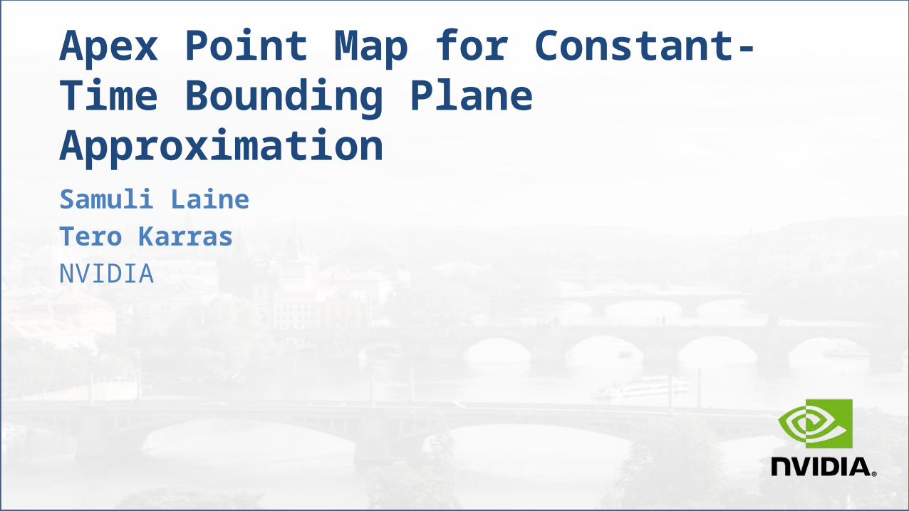
Use Case 1: Ray Tracing and Rigid Motion

Say we have a world-space BVH with leaves containing object ID + transformation matrix

Each object has apre-built BVH inmodel space

When ray finds anobject, it descendsinto per-model BVH

Use Case 1: Ray Tracing and Rigid Motion

When objects move and rotate, the world-space BVH needs to be rebuilt / refit, but per-object BVHs stay unchanged

Very fast

But: Where do we getthe world-spaceAABBs for thetransformed objects?

The Naïve Solution

Take the object’smodel-space AABB

Transform it alongwith the object

Wrap a world-spaceAABB around it

Declare victoryModel space World space

The Naïve Solution

Woefully conservative! Stats for Armadillo:

Average = 94% larger surface areathan for a tightly fit AABB

Worst case = +169% surface area

A spherical model is even worse Average = +125% AABB area Worst case = +179% AABB area

This kills the world-space BVH

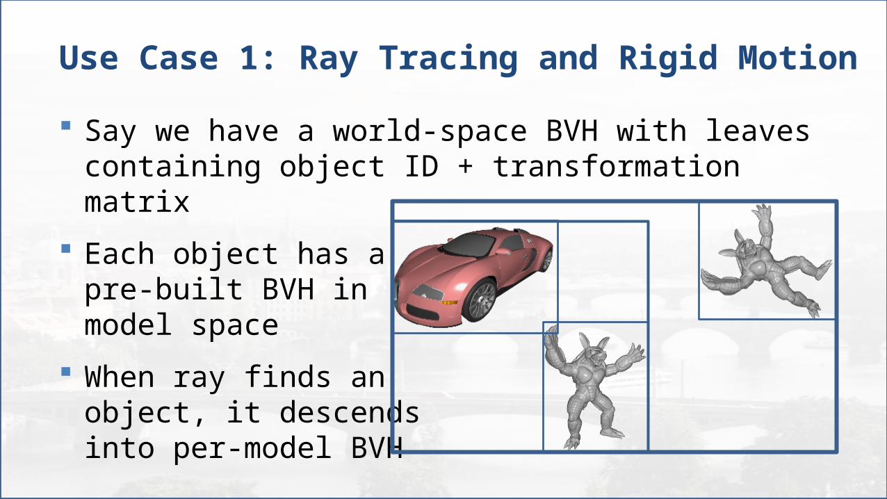
A Better Solution

Start with world-space AABB normals

Take them tomodel space

Query tightbounding plane offsets

Apply in world spaceModel space World space

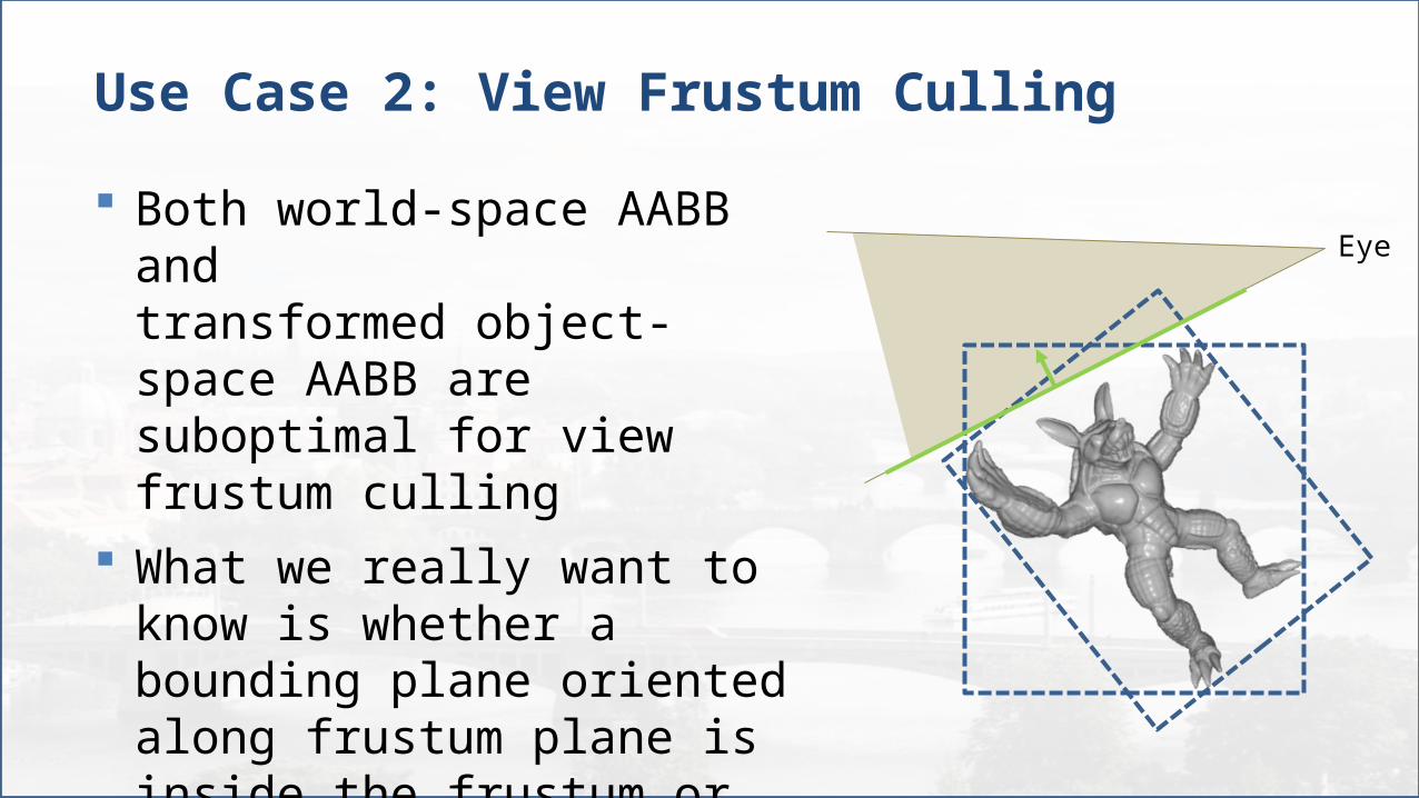
Use Case 2: View Frustum Culling

Both world-space AABB andtransformed object-space AABB are suboptimal for view frustum culling

What we really want to know is whether a bounding plane oriented along frustum plane is inside the frustum or not

Eye

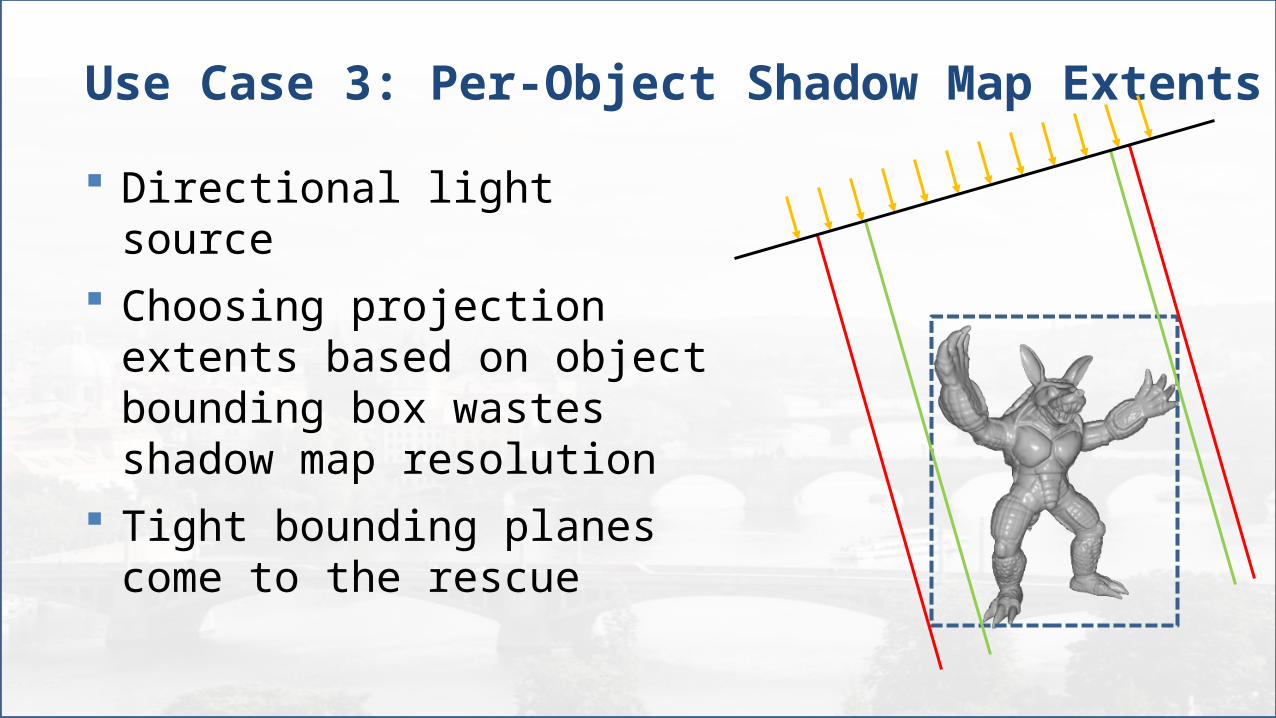
Use Case 3: Per-Object Shadow Map Extents

Directional light source

Choosing projection extents based on object bounding box wastes shadow map resolution

Tight bounding planes come to the rescue

Use Case 4: Collision Detection

Transformed object-space AABBs may intersect

Tightly fit world-spaceAABBs may intersect

But if you can guess a separating plane normal,it is very cheap to test Could try, e.g., vector

between object centers

Constraints

If we want the bounding plane fit to be fast, precalculation is unavoidable Otherwise must loop over all* vertices

Mesh needs to be static Except: See paper for extension

to skinned meshes

* Vertices on the convex hull would obviously be enough, but then we’d need to precalculate the convex hull

AABB: The Good

The amount of precalculated data is small and constant

The precalculation is fast and simple

Fitting an arbitrarily oriented bounding plane is really fast

AABB: The Bad

An arbitrarily oriented bounding plane fit to an AABB can be extremely conservative

HOWEVER

Fitting an axis-aligned plane works fine (exact result)

Fitting an almost axis-aligned plane is still okay-ish

More Is More

Why not precalculate a many-sided bounding volume?

This is known as a k-DOP Intersection of half-spaces k is the number of plane normals AABB belongs to the 6-DOP family

Determining the k plane equationsfor a mesh is easy and fast

But…

The Trouble with k-DOPs

Determining the vertices of the k-DOP surface is non-trivial, to say the least Known as the vertex enumeration problem in linear

optimization circles

2D case looks deceptively simple, problems start at 3D

k-DOP Surface Topology Is Not Fixed

A

BC

AB

C

* Except when it is (e.g., in case of AABBs)

*

Apex Point Map

Start with a k-DOP, but instead of trying to find the k-DOP surface vertices, find some other vertices These are what we call apex points

They may be k-DOP surface vertices, but possibly aren’t

In addition, choose k-DOP normals carefully so that we can easily decide a single apex point to fit the bounding plane against Makes bounding plane construction extremely fast

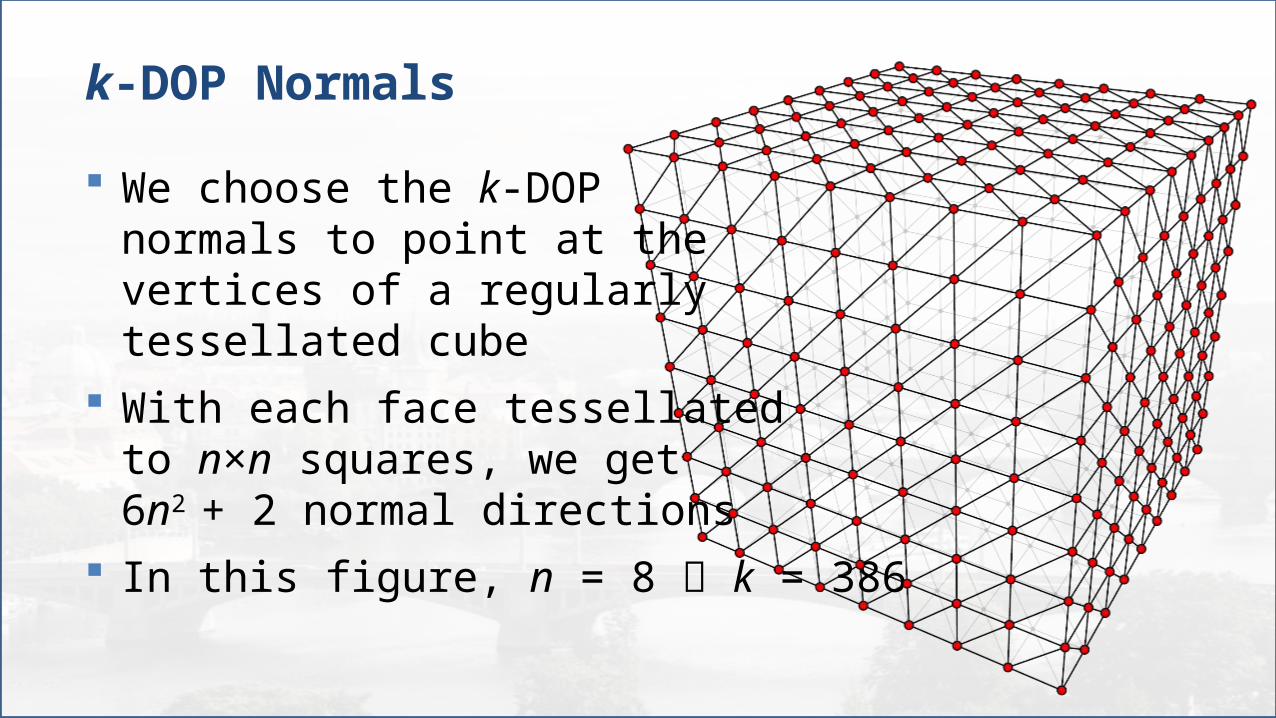
k-DOP Normals

We choose the k-DOPnormals to point at thevertices of a regularlytessellated cube

With each face tessellatedto n×n squares, we get6n2 + 2 normal directions

In this figure, n = 8 k = 386

k-DOP Normals

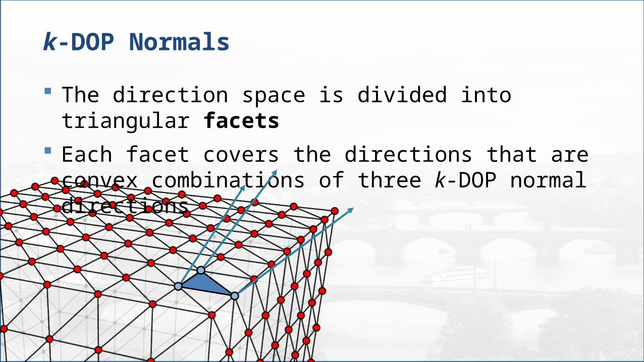
The direction space is divided into triangular facets

Each facet covers the directions that are convex combinations of three k-DOP normal directions

Constructing the Apex Point

Apex point for this facet is the intersection of the k-DOP planes that were generated using the shown normals Lies on the k-DOP surface iff corresponding k-DOP faces meet

Using the Apex Point

When fitting a bounding plane with normal in a given facet of direction space, set the plane offset so that it passes through the apex point for the facet

Why Does This Work?

k-DOP is an intersection of half-spaces Taking any subset of k-DOP planes yields a valid conservative bound for the mesh

Taking three planes yields an infinite triangular pyramid

If we’re fitting a bounding plane, we can make it pass through the apex of the pyramid – if it can bound the pyramid at all, it will bound it there too

Plane bounds the pyramid, pyramid bounds the mesh plane bounds the mesh

Summary of the Method

Precalculation: Construct a k-DOP with normals according to tessellated cube For each direction space facet, compute one apex point as the

intersection of three k-DOP planes Store these apex points, nothing else

To fit a bounding plane: Find the facet that contains the plane normal direction Fetch the apex point for the facet Set plane offset so that it passes through the apex point

Results: Quality

Results: Speed

For n=8, tops out at ~1.5M vertices / ms on NVIDIA GTX 980 Precalculated data consumes 9 KB / mesh for n=8

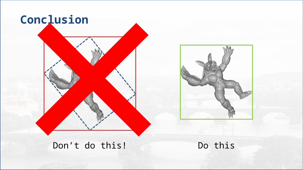
Conclusion

Don’t do this! Do this

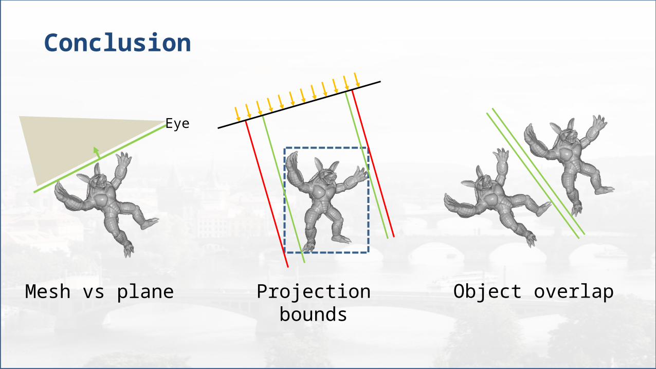
Conclusion

Eye

Mesh vs plane Projection bounds Object overlap

Thank You

Questions