APE_IM_Article_AppliedOptics_Vol47_No29_Oct10_2008_AsPublished

Dual-wavelength low-coherence instantaneousphase-shifting interferometer to measure

the shape of a segmented mirrorwith subnanometer precision

Rainer Wilhelm,1,3 Bruno Luong,1,* Alain Courteville,1 Sébastien Estival,1

Frédéric Gonté,2 and Nicolas Schuhler2

1FOGALE nanotech, 125, Rue de l’Hostellerie, 30900 Nîmes, France2European Southern Observatory, Karl-Schwarzschildstrasse 2, 85748 Garching b. München, Germany

3Current affiliation: EADS Astrium GmbH - Satellites, 88039 Friedrichshafen, Germany

*Corresponding author: [email protected]

Received 1 July 2008; accepted 6 August 2008;posted 20 August 2008 (Doc. ID 98097); published 8 October 2008

We present a noncontact optical metrology measuring the pistons and tip/tilt angles of the 61 hexagonalsegments of a compact-sized segmented mirror. The instrument has been developed within the scope of adesign study for the European Extremely Large Telescope (E-ELT). It is used as reference sensor forcophasing of the mirror segments in closed-loop control. The mirror shape is also measured by differenttypes of stellar light-based phasing cameras whose performances will be evaluated with regard to a fu-ture E-ELT. Following a description of the system architecture, the second part of the paper presentsexperimental results demonstrating the achieved precision: 0:48nmrms in piston and 74nrad rms intip/tilt. © 2008 Optical Society of America

OCIS codes: 120.3180, 120.3930, 120.3940, 120.5050.

1. Introduction

A. Cophasing of an Extremely Large Telescope

With several telescopes and stellar interferometers ofthe 8–10m diameter class in routine operation today,the research in telescope design is now focusing on so-called Extremely Large Telescopes (ELT) havingsegmented mirrors with diameters D ranging from30 to 100m. Two examples for currently runningELT projects are the European ELT (E-ELT)(D ¼ 42m, 984 segments) and the Thirty MeterTelescope (TMT, D ¼ 30m, 492 segments).A very difficult problem common to all ELTs is the

active control of the segmented primary mirror. If notactively controlled, the segments will move in a ran-

dom manner, being exposed to perturbations such asgravitational forces, wind load, and other mechanicalforces. Without controlling the segments to maintainthe shape of the mirror defined by the optical design,the spatial resolution of the telescope would be re-duced to the one of a telescope whose primary mirrorhad the diameter d of a single segment. To achieve aspatial resolution comparable to a monolithic tele-scope of large diameter D, the segmented mirror sur-face must be controlled, i.e., the segments must bephased, with an accuracy better than λ=13 rms (wave-front) [1].

During the phasing procedure, three degrees offreedom of each segment are actuated: translationalong the local optical axis (piston h) and rotationabout two axes perpendicular to the local optical axis(tip α and tilt β).

Three hardware systems are required for phasing:capacitive or inductive edge sensors providing

0003-6935/08/295473-19$15.00/0© 2008 Optical Society of America

10 October 2008 / Vol. 47, No. 29 / APPLIED OPTICS 5473

real-time information about relative segment displa-cements, segment actuators compensating for thesedisplacements, and a phasing camera. An inner fastcontrol loop using the edge sensors and the actuatorsprovides fast correction for segment displacements. Itruns continuously. Since the edge sensors only mea-sure displacements relative to a zero reference, thisreference must be provided by another sensor at reg-ular intervals (for example, at the beginning of eachnight of observation). Typically this task is performedbyaphasingcamera thatuses the light of abright stel-lar source tomeasure the shape of thewavefront. Thismethod is called optical phasing or on-sky calibration.

B. Active Phasing Experiment

Within the scope of a design study for the E-ELT, theActive Phasing Experiment (APE) aims at demon-strating activewavefront control technologies for a fu-ture ELT [2]. The experiment will validate differentstellar light-based phasing camera concepts bytesting them on a scaled-down segmented mirror,the so-called Active Segmented Mirror (ASM)(D ¼ 154mm, 61 segments). Figure 1 shows a sche-matic drawing of the ASM. Each hexagonal segmenthas a flat-to-flat distance of d ¼ 17mm. The gapwidth is approximately 70–130 μm. The total dia-meter (corner to corner) is D ¼ 154mm. The opticalsurfaces of the segments are flat [surface quality ofapproximately 50nm peak to valley (PTV)]. Eachsegment is controllable in three degrees of freedom(piston, tip, and tilt) bymeans of three piezo actuatorswithmechanical strokes of�7:5 μmand a precision indisplacement of better than 0:2nm. More detailsabout the ASM can be found in [3].Closed-loop control with a bandwidth of approxi-

mately 0:2Hz is used to apply a given pattern of pis-ton, tip, and tilt to the segments and to maintain the

ASM in this shape for a time period longer thanthe integration times of the phasing cameras(typically 1–30 s).

We present a high-precision optical metrology sys-tem that serves as the sensor in the control loop,measuring the piston, tip, and tilt of the 61 segmentsat a frequency of 4:44Hz. In addition to its role assensor in the closed-loop control, it will be used asa reference to qualify the precision of the differentphasing cameras. Following the ongoing tests atthe laboratories of the European Southern Observa-tory in Garching, Germany, APEwill be tested on-skyat a Nasmyth focus of a Unit Telescope of the VeryLarge Telescope (VLT) array on Cerro Paranal, Chile.

2. System Description of the Metrology

A. Metrology Specifications

Table 1 lists the metrology specifications. All mea-surements (piston, tip, and tilt) are performed rela-tive to the central segment whose piston is notcontrolled in closed loop. The specified measurementrange for piston (�7:2 μm) is covered by the range ofdisplacement for the piezo actuators (�7:5 μm).

The measurement is performed through a beamexpander optic (magnification factor 1=10) that isnot part of the metrology’s optical system. The beamexpander is placed between the exit pupil of the me-trology and the target (ASM). The optical path lengthbetween the exit pupil and the ASM is approximately2200mm. The optical layout of the complete APEconfiguration is shown in [2].

B. Metrology Concept

The system combines three well-established conceptsof interferometric metrology. Those are (1) instanta-neous phase-shifting interferometry, (2) low-coherence interferometry, and (3) dual-wavelengthinterferometry. We briefly explain the basics of thesethree techniques and why they have been chosen forthe present application.

Fig. 1. ASM with 61 segments, each equipped with three piezoactuators. The flat-to-flat distance of a single segment isd ¼ 17mm. The total diameter of the mirror (corner to corner)is D ¼ 154mm.

Table 1. Achieved Specifications of the Metrology

Item Specification

Measurement range for pistona �7:2 μmMeasurement range for tip/tiltb �250 μradWorking distancec 2200mmPiston precision (closed loop) 0:48nmrmsTip/tilt precision (closed loop) 74nrad rmsMeasurement frequency 4:44HzClosed-loop bandwidth 0:2HzFrame-to-frame time difference 25ms

aThe piston range is defined with respect to the piston of thecentral segment.

bThe tip/tilt range is defined at the level of the target(i.e., the ASM).

cThe working distance is the distance between the exit pupil ofthe metrology and the target (ASM).

5474 APPLIED OPTICS / Vol. 47, No. 29 / 10 October 2008

1. Instantaneous Phase-Shifting Interferometry

Phase-shifting interferometry (PSI) determines thephase difference between two interfering beams bymeasuring the irradiance of the interference fringesas the phase difference between the beams’ changesin a known manner. Besides the phase differencethere are two other unknowns to be determined bya PSI algorithm: the amplitude of the probe beamand the amplitude of the reference beam. Since thereare three unknowns, at least three irradiance mea-surements have to be made. To reduce measurementerrors, four or more measurements are made. Typi-cally the phase is changed by 90° between two conse-cutive measurements, but there also exist PSIalgorithms using phase shifts different from 90°.The phase shifts between consecutive measurementsare created by a phase shifter—typically amoving re-ference mirror in a delay line or an electro-optic mod-ulator that varies the phase of the reference beam in acontrolled way. Awide variety of PSI algorithms existand are described in the literature [4–6].In the presence of vibrations and air turbulence,

changing the reference beam phase in a controlledmanner can become very difficult. The mentionedperturbations, which will certainly be present on atelescope platform, can change the phase differencebetween two beams in unknown ways and thereforecan cause large errors in the measurement. This pro-blem can be avoided by using the technique of instan-taneous PSI (also referred to as snapshot or singleshot interferometry). Four interferograms at phaseshifts of 90° are simultaneously acquired, i.e., with-out any time lag between measurements. Several ofsuch snapshot interferometers have been demon-strated [7–9]. We have chosen a concept where thephase shifts are induced by polarizing optical ele-ments such as polarizing beam splitters and phaseretarders (wave plates). The four interferogramsare detected on four CCD cameras. An accurate pixel-to-pixel correlation between the different cameras isobtained by an image-matching method.

2. Low-Coherence Interferometry

Low-coherence interferometry performs interfero-metric measurements using the light emitted froma relatively broadband source with a coherencelength of typically a few tens of micrometers. Theterm “coherence” refers to the temporal coherenceof the light. The most frequently used light sourcefor this type of interferometer is a superluminescentdiode (SLD). The metrology system also uses thistype of source.A low-coherence interferometer works as a com-

parator of optical group delays, i.e., products of grouprefractive index and geometrical distance. The groupdelay in the probe arm of the interferometer is com-pared to the group delay of the reference arm, whoselength can be varied using amovable referencemirrorin a delay line. Expressed as a function of the refer-ence mirror position, the interferometric signal is a

sinusoidal fringe pattern with a fringe period equalto half the optical wavelength λ. The pattern is modu-lated by an envelope that is proportional to the Four-ier transform of the source frequency spectrum. Forthe approximately Gaussian spectrum of an SLD,the envelope has a Gaussian shape too. Its width isthe round-trip coherence length lc ¼ 2 lnð2Þλ2=ðπδλÞ,where λ and δλ are the center wavelength and the fullspectral width at half maximum of the source, respec-tively. Themaximum of the fringe envelope occurs fora group delay difference (GDD) of zero between thetwo arms.

The twoSLDsused in themetrology systemoperateat wavelengths λ1 ≈ 834:6nm and λ2 ≈ 859:6nm, eachwith a spectral bandwidth of δλ ≈ 13:5nm. This corre-sponds to a round-trip coherence length of lc ≈ 23 μm.Since during an extended measurement run lastingseveral hours the group delays in the two interferom-eter arms might vary in a different way due to tem-perature variations, the operational point of thesystemmight drift away from the initial optimum po-sition of GDD zero to a position with lower fringe con-trast. To increase this working range, we use spectralfilters to reduce the bandwidth of each SLD to a valueof δλ ≈ 3:2nm.This yields a significantly larger round-trip coherence length of lc ≈ 100 μm.

The advantages of a low-coherence interferometerwhen compared to a classical laser interferometerare the fact that the measurement is less affectedby speckle noise and that parasitic internal reflec-tions do not perturb the coherent signal.

3. Two-Wavelength Interferometry

AllPSIalgorithmsmeasure the interferometricphasemodulo 2π. Phase unwrapping is necessary to gener-ate a continuous phase distribution that can beconverted into a surface height profile.Whenmeasur-ing at a single wavelength λ, the range of nonambigu-ity for distance measurements is given by λ=2 since adisplacement of the target or the reference mirror byΔz ¼ λ=2 creates an optical path difference (OPD) of λ,i.e., creates a phase shift of 2π. An important precon-dition for any phase unwrapping algorithm is that thephase difference between two measurements (eitherseparated in space or in time) is smaller than thethreshold of the phase unwrapping algorithm (whichis typically equal to π). This means that steps or dis-continuities (in space or in time) larger than λ=4—thepath difference corresponding to a phase difference ofπ—will cause the phase unwrapping algorithm tobreakdown.The fringeorder is lost over the step (tem-poral or spatial). In our segmentedmirrorapplication,spatial discontinuities larger than λ=4 exist at thesegments’ borders. Two-dimensional spatial phaseunwrapping is not suitable.

The technique of two-wavelength interferometryallows the fringe order to be determined and canmeasure step heights and discontinuities much lar-ger than a quarter optical wavelength. The rangeof nonambiguity increases to Λs=2, where Λs is the


synthetic wavelength defined as

Λs ¼λ1λ2

jλ1 − λ2j; ð1Þ

with λ1 and λ2 denoting the two individual wave-lengths.With λ1 ≈ 834:6nm and λ2 ≈ 859:6nm, the range of

nonambiguity of the interferometer becomesΛs=2 ≈ 14:4 μm, which corresponds to twice the mea-surement range for piston (see Table 1). Themeasure-ment range is compatible with the range of the piezoactuators.

C. Functional Description of the Metrology System

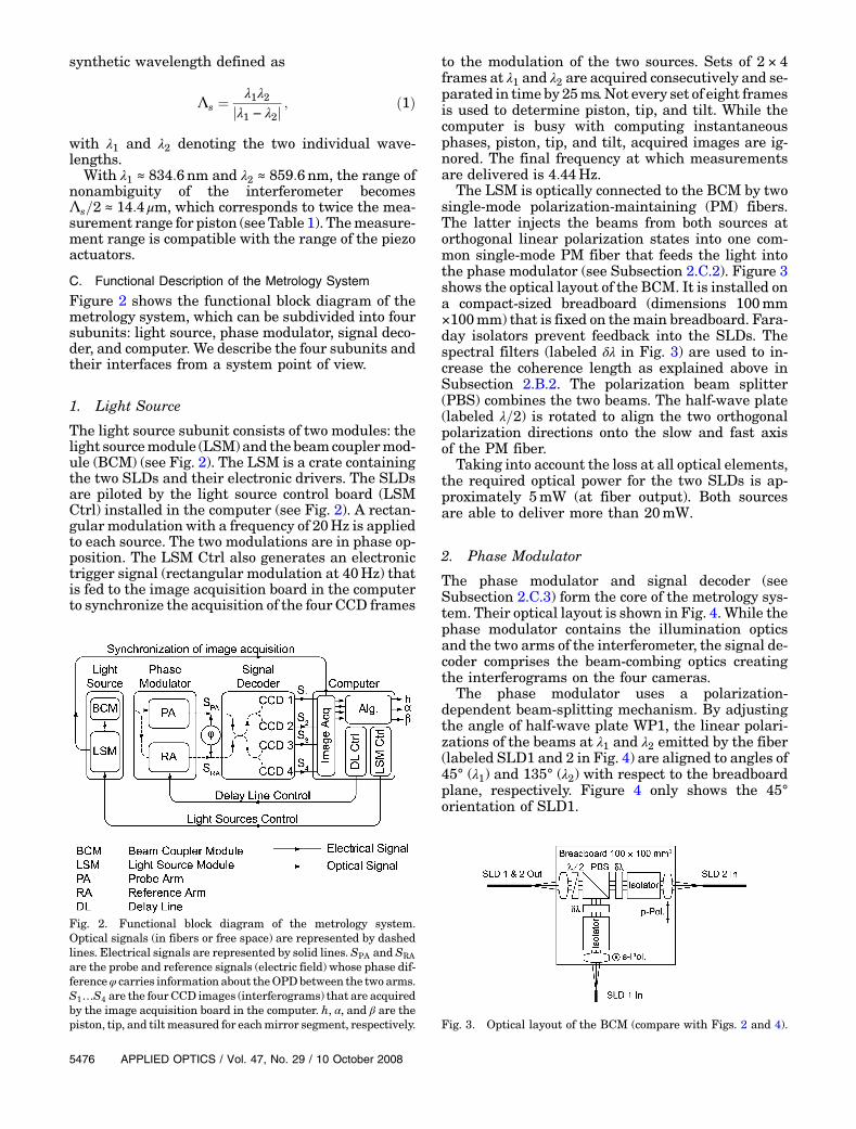
Figure 2 shows the functional block diagram of themetrology system, which can be subdivided into foursubunits: light source, phase modulator, signal deco-der, and computer. We describe the four subunits andtheir interfaces from a system point of view.

1. Light Source

The light source subunit consists of two modules: thelight sourcemodule (LSM) and the beamcouplermod-ule (BCM) (see Fig. 2). The LSM is a crate containingthe two SLDs and their electronic drivers. The SLDsare piloted by the light source control board (LSMCtrl) installed in the computer (see Fig. 2). A rectan-gular modulation with a frequency of 20Hz is appliedto each source. The two modulations are in phase op-position. The LSM Ctrl also generates an electronictrigger signal (rectangular modulation at 40Hz) thatis fed to the image acquisition board in the computerto synchronize the acquisition of the four CCD frames

to the modulation of the two sources. Sets of 2 × 4frames at λ1 and λ2 are acquired consecutively and se-parated in time by 25ms.Not every set of eight framesis used to determine piston, tip, and tilt. While thecomputer is busy with computing instantaneousphases, piston, tip, and tilt, acquired images are ig-nored. The final frequency at which measurementsare delivered is 4:44Hz.

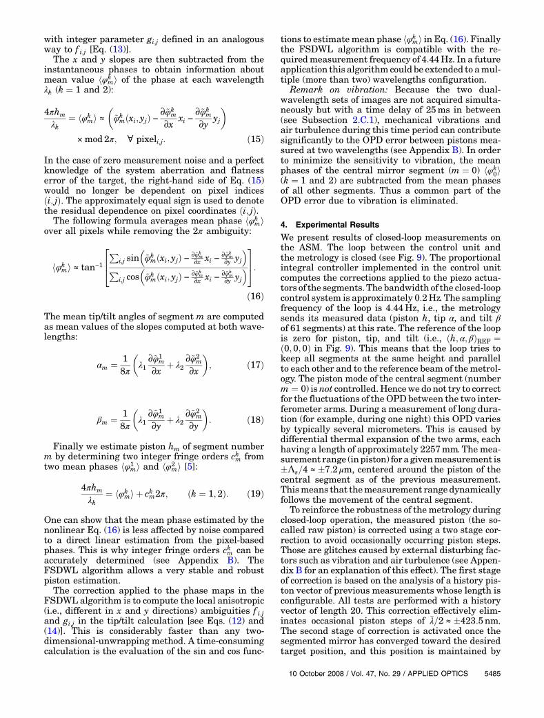
The LSM is optically connected to the BCM by twosingle-mode polarization-maintaining (PM) fibers.The latter injects the beams from both sources atorthogonal linear polarization states into one com-mon single-mode PM fiber that feeds the light intothe phase modulator (see Subsection 2.C.2). Figure 3shows the optical layout of the BCM. It is installed ona compact-sized breadboard (dimensions 100mm×100mm) that is fixed on themain breadboard. Fara-day isolators prevent feedback into the SLDs. Thespectral filters (labeled δλ in Fig. 3) are used to in-crease the coherence length as explained above inSubsection 2.B.2. The polarization beam splitter(PBS) combines the two beams. The half-wave plate(labeled λ=2) is rotated to align the two orthogonalpolarization directions onto the slow and fast axisof the PM fiber.

Taking into account the loss at all optical elements,the required optical power for the two SLDs is ap-proximately 5mW (at fiber output). Both sourcesare able to deliver more than 20mW.

2. Phase Modulator

The phase modulator and signal decoder (seeSubsection 2.C.3) form the core of the metrology sys-tem. Their optical layout is shown in Fig. 4. While thephase modulator contains the illumination opticsand the two arms of the interferometer, the signal de-coder comprises the beam-combing optics creatingthe interferograms on the four cameras.

The phase modulator uses a polarization-dependent beam-splitting mechanism. By adjustingthe angle of half-wave plate WP1, the linear polari-zations of the beams at λ1 and λ2 emitted by the fiber(labeled SLD1 and 2 in Fig. 4) are aligned to angles of45° (λ1) and 135° (λ2) with respect to the breadboardplane, respectively. Figure 4 only shows the 45°orientation of SLD1.

Fig. 2. Functional block diagram of the metrology system.Optical signals (in fibers or free space) are represented by dashedlines. Electrical signals are represented by solid lines. SPA and SRAare the probe and reference signals (electric field) whose phase dif-ferenceφ carries information about theOPDbetween the two arms.S1…S4 are the fourCCD images (interferograms) that are acquiredby the image acquisition board in the computer. h, α, and β are thepiston, tip, and tiltmeasured for eachmirror segment, respectively. Fig. 3. Optical layout of the BCM (compare with Figs. 2 and 4).


The polarizing beam splitter cube PBS1 splits thebeam into the two arms of the interferometer, i.e., theprobe arm (toward the ASM) and the reference arm(toward the reference mirror on the translationstage). The external distance of approximately2200mm between the exit pupil (top right in Fig. 4)and the ASM is reproduced internally in the delayline with its folded mirror design.Quarter-wave plates (WP2 and WP3), both or-

iented at 45°, transform the outgoing linear polariza-tions [perpendicular (s) for the reference arm andparallel (p) for the probe arm] into circular ones. Re-flection on the final surface in each arm (ASM in theprobe arm and reference mirror in the reference arm)inverses the handiness of the polarization. After hav-ing passed the quarter-wave plates for a second time,the polarizations are converted back to linear, ro-tated by 90° relative to the outgoing beams, beforerecombination on PBS1. This circulator-type setupoptimizes the total power throughput.After recombination on PBS1 the probe and refer-

ence beams have mutually perpendicular polariza-tions. The pair of beams with a phase shift φ carrythe information about theOPD between the two armsthat one wants to measure.A scan of the linear translation stage carrying the

referencemirror is performed for calibrationpurposes(see Section 3.D). During the actual measurementsthe reference mirror is kept fixed at one position that

corresponds to equal optical group delays in botharms, i.e., to the maximum of the fringe envelope.

3. Signal Decoder

The signal decoder directs the recombined beamsleaving the phase modulator at orthogonal linear po-larizations via respectively separate paths onto fourCCDs. Thanks to the optical design each CCD has adifferent “sensitivity” to the information contained inthe combined beams. The first step consists of rotat-ing linear polarizations s and p leaving the phasemodulator by 45° using the half-wave plate WP4 or-iented at 22:5°. Then the nonpolarizing beam splitterBS cube directs the pair of beams to the two pairs ofCCDs (CCD1 & 2 and CCD3 & 4). The quarter-waveplateWP5 has its crystal axis oriented parallel to oneof the two beams, i.e., it introduces an additionalphase shift of 90° between probe and referencebeams for the interferograms on CCD1 and 2. Sinceat the entrance of PBS2 and PBS3 the linear polar-izations of the two beams are oriented at 45° and135°, each beam is equally divided into a parallel(p) and a perpendicular (s) component, propagatingtoward the two CCDs assigned to each beam splittercube. Finally the two interferograms observed oneach pair of CCDs are opposite in phase. The four in-terferograms on CCD1;…; 4 are in phase quadra-ture, which means that they are shifted in phase

Fig. 4. Optical layout of the interferometer. The dimensions of the rectangular breadboard are 1200mm× 600mm. The internalmagnification between the exit pupil (top right) and each of the CCDs is Mint ¼ 1=3. The segmented mirror is imaged onto the exit pupilby a beam expander (not shown here) with magnification of Mext ¼ 1=10. The gray squares represent the local state of polarization. Thepolarization of the probe beam is represented by a solid line, while the polarization of the reference beam is represented by a dashed line.A closer look to the BCM is provided in Fig. 3.


by 90° with respect to each other. Their image acqui-sitions are synchronized.

4. Computer

The computer hosts the three electronic boards tocontrol the light sources, the translation stage inthe delay line, and the four cameras (see Fig. 2). Italso runs the algorithms for image matching,calibration, and phase detection.

D. Optical Design

Figure 4 shows the optical layout of the interferom-eter. Optics and optomechanics are installed on an op-tical breadboard of dimensions 1200mm× 600mm.For the APE experiment the metrology breadboardis fixed by a three-point kinematic support on top ofthe main APE optical table. To avoid the disturbingeffects of air turbulence, protective covers encloseboth the metrology and the whole APE setup (for de-tails about APE see [2]).The optical design uses all lenses in telecentric re-

lay configurations. This ensures a homogeneous illu-mination on the segmented mirror (within the limitsof a clipped Gaussian beam profile) and makes thealignment of the system easier. Most of the opticalcomponents have either a 1 or 2 in: diameter(1 in: ¼ 2:54 cm). All lenses are 2 in: in diameter toensure diffraction-limited imaging quality.The optical interface between the metrology sys-

tem and the external optical system of the APE ex-periment is an image of the segmented mirror (scalefactor 1=10). A beam expander, formed by the combi-nation of an off-axis parabola and a lens (not shownin Fig. 4), creates this image that is located in the exitpupil of the metrology at the upper right border of itsbreadboard.The target, i.e., the segmented mirror, is illumi-

nated by a collimated beam with perpendicular inci-dence. The circular aperture stop (diameter 15:4mm)shown in Fig. 4 (in front of WP1) is imaged on the exitpupil and on the target where it has a diameter of154mm. It clips the illuminating Gaussian beamat approximately half its waist radius, correspondingto an irradiance level equal to 60% of the peak irra-diance. The metrology-internal magnification factorbetween the exit pupil and each of the CCDs is1=3. With a magnification factor of 1=10 betweenthe target and its image in the exit pupil, the totalmagnification becomes 1=30.The segmented mirror is imaged onto the four

CCDs with diffraction-limited quality. Each CCDhas768 × 580 squarepixels. Thenumber of pixels con-tained in the image of a singlemirror segment is 3581.TheAiry disk diameter isDAiry ≈ 20:8 μm, correspond-ing to 2.5 pixels on theCCD (at themeanwavelength).Image distortion is negligible with a maximum valueof −0:05% at the corner of the CCD image, whichcorresponds to −0:0005 × 15:4=2mm ≈ 3:9 μm—

approximately half a pixel’s dimension. The fiveSeidel aberrations are all below 0:3λ with astigma-tism as the most important contribution.

Diffraction effects on the reference beam are signif-icantly reducedby creatingan intermediatepupil (im-age of the aperture stop) using two lenses in afocalconfiguration (see Fig. 4). Hence the collimated beampropagation distance responsible for diffraction ef-fects on the reference beam is significantly smallerthan 2 × 2200mm (round-trip). With an initial beamdiameter of 15:4mm, near-field diffraction effects (in-crease in beam diameter, ripples on the electric fieldamplitude profile, and curvature of wavefront) of theclipped Gaussian beam remain small.

The numerical aperture of the system is large en-ough to capture a maximum tip/tilt angle ofγmax ¼ 0:8mrad—a range significantly larger thanthe maximum measurable tip/tilt of �250 μrad (seeTable 1).

3. Algorithms for Interferometric Image Processing

Starting with a description of the interferometric sig-nal, we discuss the methods and algorithms used toobtain a surface height measurement from the 2 × 4interferograms. Our description includes topics suchas calibration, image matching, instantaneous phasemeasurement, and determination of piston, tip, andtilt by a dual-wavelength algorithm.

A. Interferometric Signal and Instantaneous Phase

We use notations ðx; yÞ and zðx; yÞ for a position in thetransverse plane of the target, i.e., the segmentedmirror, and the corresponding surface height. Eightinterferometric signals fIki g are created for surfaceheight z. The signals are acquired by four camerasCCDi (i ¼ 1;…; 4) for two wavelengths λk (k ¼ 1and 2). The irradiance of each interferometric signalcan be written as

Iki ðx; yÞ ¼ Bki ðx; yÞ þ Ak

i ðx; yÞ sin½φkðx; yÞ þ θki ðx; yÞ�;ð2Þ

where φkðx; yÞ≡ 4πzðx; yÞ=λk mod 2π is the wrappedinterferometric phase measured at wavelength λk;Bk

i ðx; yÞ is the background, i.e., the incoherent sumof irradiances of both reference and probe arm;Ak

i ðx; yÞ is the amplitude of the sinusoidal interfero-metric signal; and θki ðx; yÞ is the reference phase as-sociated to CCDi. Among these four quantities onlythe phases φkðx; yÞ contain information about surfaceheight zðx; yÞ. Since the phase φkðx; yÞ is measured atthe same time on the four CCDs, we refer to it as theinstantaneous phase. Note that the term “instanta-neous” refers to the four cameras but not to thetwo wavelengths. As stated in Subsection 2.C.1,the acquisitions at λ1 and λ2 are separated by a timelag of 25ms.

B. Operational Procedures Overview

During the measurement procedure the referencemirror in the delay line is kept at a fixed position cor-responding to a GDD of zero between the two arms(see Subsection 3.E). The systemacquires the 2 × 4 in-terferograms Iki [Eq. (2)] and computes instantaneous


phases φkðx; yÞ for both wavelengths (k ¼ 1 and 2) atthe measurement frequency of f ¼ 4:44Hz. The twophase maps are then used to calculate the piston(h), tip (α), and tilt (β) of each mirror segment. Inclosed-loop operation these data ðh; α; βÞ are sent tothe controller computing the commands applied tothe piezo actuators of each segment in order to bringthe mirror into the desired shape. The algorithm toderive the piston, tip, and tilt from the two phasemaps has been specifically developed for the presentapplication of segmented mirror metrology and ispresented in Subsection 3.E.4.The three other quantities, Bk

i ðx; yÞ, Aki ðx; yÞ, and

θki ðx; yÞ, affecting interferograms Iki vary rather slowlyduring the measurement, at a typical time scale of afew hours. The variations are mainly due to tempera-ture drifts. They do not depend on surface height z.Both the background and the amplitude depend on ir-radiances Iki;probe and Iki;ref of the probe and referencearms, respectively:

Bki ðx; yÞ ¼ Iki;probe þ Iki;ref ; ð3Þ

Aki ðx; yÞ ¼ 2ðIki;probeIki;ref Þ1=2: ð4Þ

The fringe visibility (or contrast) Vki ðx; yÞ is defined as

the ratio of fringe amplitude over background: V ¼A=B with a maximum value of V ¼ 1 for equal irra-diances Iki;probe ¼ Iki;ref . To maximize the signal-to-noise ratio, it is important to obtain the highestpossible fringe visibility, i.e., to equalize as much aspossible the contributions of the probe and referencearms. This equilibrium must be respected simulta-neously for all four CCDs and at both wavelengths.In our case we obtain a fringe visibility varyingbetween 0.6 and 0.7 depending on pixel location,CCD, and wavelength.In instantaneous PSI it is not necessary to know

the absolute reference phase θki ðx; yÞ for each CCD;nevertheless the three phase shifts between the fourinterferograms must be known precisely. By conven-tion we assume the reference phase of the first CCDto be zero at both wavelengths, i.e., θk1ðx; yÞ ¼ 0 fork ¼ 1 and 2. Hence the reference phases of the re-maining three CCDs correspond to the phase shiftswith respect to the interferogram on CCD1.An accurate determination of the three quantities

background, amplitude, and phase shift is an essen-tial step to be performed prior to the measurement.This is the main purpose of the calibration proceduredescribed in Subsection 3.D. In contrast to the mea-surement procedure, the calibration is performedusing a series (stack) of images (each ofwhich is calledan image frame) acquired at different positions of thereference mirror in the delay line. Notice that back-ground Bk

i ðx; yÞ and amplitude Aki ðx; yÞ also depend

on the power of the light sources. This dependencyis essentially a first-order law for both backgroundand amplitude, and the remaining variations will

be further removed during the measurement. In ad-dition the amplitude depends on the GDD betweenthe two arms, i.e., the positionwithin the fringe envel-ope. The amplitude is monitored continuously duringthe measurement. Differential temperature varia-tions occurring during a measurement run canchange the GDD. The operational points move awayfrom the envelope’s maximum, leading to a decreasein fringe amplitude (and contrast). If the contrast getsbelow a predefined threshold, a recentering is per-formed: After a scan to determine the new positionof GDD zero, the reference mirror is moved to thisposition.

Finally the four CCD images must be matched bysoftware, i.e., finding the pixels on the four differentCCDs that correspond to same physical location onthe target. This matching procedure must be per-formed at a very high accuracy (about a tenth of apixel size). We discuss the requirement on matchingaccuracy in more detail in Subsection 3.D.3.

C. Determining the Optimum Delay Line Position

The search for fringes is performed in two steps. Dur-ing a first coarse scan, the reference mirror is movedat a faster speed over a course of a few centimeters todetect theposition corresponding to a large irradiancevariation. A second fine scan at a slower speed is per-formed in the interval around the position deter-mined during the coarse scan. The length of thisinterval is chosen to match the coherence length,i.e., 100 μm. The scan velocity is adjusted such thatthe fringes are acquired with a sampling of λ=8 ¼π=2 between two consecutive images. A PSI demodu-lation method (as described in Subsection 3.D.2) isthen applied to compute the fringe amplitude, i.e.,fringe envelope. Themaximumof theGaussian envel-ope (zero GDD) is detected by standard curve fittingprocedures. There exists a GDD zero position for eachwavelength. They are separated by approximately afew tens of micrometers due to a differential groupdispersion in the two arms of the interferometer:The types and thicknesses of optical glasses in thetwo arms do not match each other exactly. The probearm contains the beam expander, which itself com-prises a lens, while the reference arm contains twolenses. The delay line position is then chosen as theaverage of the two optimum positions at λ1 and λ2.A planned future improvement is a full dispersioncompensation by inserting a flat piece of glass inthe reference arm. This would let the two GDD zeropositions for λ1 and λ2 coincide, i.e., further optimizethe fringe contrast.

D. Calibration Methods and Algorithms

1. Calibration Workflow

The calibration startswith the referencemirror in thedelaylineatitszeroGDDposition(seeSubsection3.C).First the optical power of both SLDs is adjusted suchthat the full dynamical range of theCCDs is exploited.Then the four cameras acquire a stack of imageswhile


the translation stage performs a fine scan centeredaround the zero GDD position. The matching algo-rithm determines the matching parameters for thefour images. Camera phase differences θiðx; yÞ (i ¼ 2,3, and 4) are calibrated using a PSI algorithm. Back-groundBk

i ðx; yÞ and fringe amplitude Aki ðx; yÞ are cali-

brated for eachpixel of all four cameras.A tessellationby software on thematched image is carried out by de-termining the subset of pixels belonging to eachsegment.

2. Temporal Demodulation by Delay LineScanning

As mentioned in Subsection 3.D.1, during the cali-bration a stack of images is acquired at different po-sitions of the reference mirror. The step size ordistance between two adjacent positions of the refer-ence mirror is imposed by the PSI algorithm used toestimate the phases of the four interferograms bytemporal demodulation of the fringes. The most com-mon phase shift in PSI is π=2, corresponding to a stepsize of λ=8 ¼ 104:3nm at λ1 ¼ 834:6nm.Two solutions could be envisaged: (1) moving the

reference mirror to a series of standstill positions se-parated by the required step size or (2) continuousacquisition of image frames while the reference mir-ror is moving at constant velocity. To our knowledgethere exists to date no commercially available trans-lation stage that is able to move to a standstill posi-tion with a positioning accuracy of a few nanometers(a small fraction of the step size). Therefore ourdesign choice is of the second option (2).With an image acquisition frequency of f ¼ 25Hz,

to acquire two consecutive frames separated by aphase of π=2 (i.e., for a displacement of Δz ¼ λ=8),the translation stage motor must be able to moveseamlessly at the speed of v ¼ λ=8 × f . Forλ1 ¼ 834:6nm, v ¼ 2:61 μms−1, and λ2 ¼ 859:6nm,v ¼ 2:69 μms−1. The chosen translation stage(MICOS PLS-85) has been successfully tested witha velocity as low as 0:1 μms−1 [10].Even though the translation stage is commanded

to move at constant velocity, the real instantaneousvelocity might fluctuate significantly around thenominal value. Because of this velocity variation,the positioning error of the reference mirror andits effect on the fringe demodulation has to be stu-died with great attention.The displacement of the MICOS PLS-85 at small

velocities in the required range has been measuredwith a high resolution of a few nanometers using alaser interferometer [10]. The residual linearity error(i.e., the deviation of the position-versus-time curvefrom a straight line fit through the data) has a PTVamplitude of approximately �100nm.We have considered the Hariharan five π=2 step al-

gorithm [4] for the demodulation. Among multistepphase-shifting algorithms with maximum of fivesteps, Hariharan’s method is much less sensitive tothe error of phase sampling (even for a fairly large

sampling error), i.e., to position error of the transla-tion stage. In practice more than five frames are ac-quired during calibration. The demodulationalgorithm will be applied on a sliding five-step win-dowmoving over all frames. The phase shifts betweenCCDs are estimated by averaging the demodulationresults applied on the individual sliding window.

We used themeasured typical-linearity error of thetranslation stage to numerically analyze the error ofthe phase shifts estimated by demodulation. The sys-tematic errors of the phase shift with respect to thenumber of CCD frames is represented in Fig. 5. Weobserve that the systematic errors do not improvesignificantly by using more than 12 frames. In ourcase, including a safety margin, we chose to acquire20 frames.

Additionally we have studied a more sophisticateddemodulation algorithm also using five π=2 steps. Ap-pendix A explains whywe have chosen this algorithmas the preferred solution in the final implementationof the software for the fringe demodulation during thecalibration.

As mentioned above, the phase shifts between thefour cameras will be calibrated by continuously mov-ing the reference mirror. The optical design shouldyield phase shifts that are spatially constant overthe beam diameter, i.e., that do not depend on posi-tion ðx; yÞ. Their theoretically expected values are

ðθ1; θ2; θ3; θ4Þ ≈�0; π; π

2;−

π2

�

for both wavelengths since the polarizing elements(beam splitters and wave plates) are achromatic overthis range.

Experimentally we observe, however, noticeablespatial variations of phase shifts θki ðx; yÞ across theðx; yÞ plane. The variations have a PTV amplitude

Fig. 5. Systematic error for the calibration of phase differencesbetween CCDs due to the nonuniformity of the translation stagemovement for the three phase differences as a function of the num-ber of CCD frames used.


of a few degrees. For example, Fig. 6 shows phaseshift θ12ðx; yÞ (at λ1) between CCD2 and CCD1. Onthe left-hand side, the raw phase shift is shown(PTV ≈ 20°). The large variations only occur at highspatial frequencies. Smooth low spatial frequencycomponents of the phase-shift distribution havePTV values from 2° to 7° depending on which pairof CCDs is considered. In our software implementa-tion we project the phase-shift map into a piecewiseconstant phase shift having a one single phase-shiftvalue per segment and per CCD. The piecewiseconstant map will be used during the measure-ment to compute the instantaneous phases (seeSubsection 3.E.2).We also considered a self-calibration method based

on a two-dimensional Fourier-Hilbert demodulationtechnique. It determines the phase shifts directlyfrom the interferograms without the need to stepthrough the phase of each one [11]. Even though thisattractive method works well most of the time, oursimulations indicate that it can fail to estimate withsufficient accuracy when using four interferograms,sometimes with an error of estimated phase shiftthat can be as high as 6°. Note that the self-calibra-tion method would work seamlessly with a minimumof five interferograms, which unfortunately is notcompatible with the architecture of our system usingfour cameras.

3. Matching of the Four Images

The calibration and measurement algorithms rely onthe knowledge of the matching of the four-pixel gridson the four CCDs with physical positions ðx; yÞ on thesegmented mirror. Even after very careful alignmentof the optical elements, the images on the four CCDswill not be completely matched, i.e., four pixels with

the same pixel coordinates ði; jÞ on the four CCDframes will not correspond to the same physical loca-tion ðx; yÞ on the target. The four images will differ inrotation, translation, and their relative scaling.While rotation and translation are mainly due to re-sidual imperfections of the mutual alignment of thefour cameras, the different image sizes correspond toslightly different magnification factors that arecaused by tolerances on the focal distances of theimaging lenses (typically of the order of 1%). The op-tical design ensures that image distortion is negligi-ble (see Subsection 2.D). Therefore an affinetransformation (a combination of rotation, trans-lation, and scaling) is enough to match the imagesaccurately.

During the calibration the images are matchedautomatically by detecting the polygonal contour ofthe fringe visibility V ¼ A=B. The visibility mapsare computed separately for each stack of images ac-quired for each CCD. Then the polygonal vertices arenumerically extracted and compared with the theo-retical locations of vertices (i.e., without affine trans-formation). The affine transformation parameters(there are four for each CCD: scaling, rotation angle,and two lateral shifts) of the image are computedfrom the absolute differences in position for two setsof vertices, numerically detected and theoretical. SeeFig. 7 for an illustration of matching using the con-tour of the fringe visibility.

The precision of the matching is directly linkedto the maximum measurable tip/tilt (compare withTable 1). The smaller the matching error, the largerthe maximummeasurable tip/tilt. For a given combi-nation of matching error and tip/tilt angle, the sys-tematic error obtained for the interferogram phaseon one CCD is

Fig. 6. Phase shift (θ2) between CCD2 and CCD1. On the left-hand side is the raw phase-shift, and on the right-hand side is a constantpiecewise phase shift per segment that is effectively used to compute the instantaneous phases during the measurement step.


δθ ¼ 4πλ

ΔpMtotal

δx ·GTT; ð5Þ

where Δp is the CCD pixel linear dimension (hereΔp ¼ 8:3 μm), Mtotal is the optical magnification ofmetrology and external beam expander (hereMtotal ¼ 1=30), δx is the matching error vector in unitof pixels, and GTT is the height gradient vector of thetarget, which equals to GTT ¼ ðα; βÞ for small tip/tiltangles. The dot denotes a scalar product of twovectors.A too large product δx ·GTT degrades the precision

of the metrology system in two ways. First the phasedifferences between the different pairs of CCDs can-not be accurately estimated during the calibration.The phase error δθ affects reference phase θki inEq. (2) associated to each CCD. Second the determi-nation of the instantaneous phase φk from four inter-ferograms is also affected by the matching-inducedphase error δθ. Consequently, periodic systematic er-rors in the OPD measurements at both wavelengthswill increase (compare with Section 4). The metrolo-gic precision degrades.By means of a specific test using a flat reference

mirror on a tip/tilt stage that replaced the segmented

mirror as target, we have determined the maximummeasurable tip/tilt angle to be 250 μrad (see Table 1).Simulations using images with typical noise levelshave shown that our algorithm can achieve an errorof matching of jδxj ¼ 0:1pixel. Inserting those twoquantities into Eq. (5), we can estimate the phase-shift error in this border case to be 5:4° (singleCCD at λ1 ¼ 834:6nm).

Once the matching parameters have been found,the images are matched using an interpolationscheme. An interpolated value depends on the valuesof 16 ¼ 4 × 4 neighboring pixels (see Fig. 8). The un-derlying irradiance function Iðx; yÞ is approximatedwith a tensorial bicubic polynomial interpolationscheme that provides a good accuracy of interpola-tion of the oscillating part of the signal intensity:

Iðx; yÞ ¼Xp;q

apqxpyq; with ðp; qÞ ¼ 0;…; 3:

The 16 coefficients fapqg are computed uniquely so asto interpolate image irradiances Iði;jÞ at the 16 neigh-boring pixels ði; jÞ.

Fig. 7. Matching of the images using the contour line of the fringe contrast (white polygonal curves). The vertices of this polygon areextracted and matched to ideal positions of the vertices (cross markers). The original image (left) is matched to an ideal image (withouttransformation) by using a bicubic polynomial scheme (right).


E. Measurement Algorithms

1. Workflow in the Measurement Loop

The first task in the measurement loop is the acqui-sition of eight images Iki ðx; yÞ at both wavelengths(k ¼ 1 and 2) on the four CCDs (i ¼ 1;…; 4). Thisis followed by a bicubic interpolation of the imagesto match the pixels to the same physical locationon the segmentedmirror. Then instantaneous phasesφkðx; yÞ are computed for both wavelengths. Finallythe system calculates the synthetic phase (piston),tip, and tilt for all segments using a dual-wavelengthalgorithm. In closed-loop operation the data are sentcontinuously to the controller via the main networkof the APE experiment (see Fig. 9).

2. Determining the Instantaneous Phase fromFour Interferograms

From Eq. (2) we first compute the normalized irra-diances for each camera CCDi (i ¼ 1;…; 4) and eachwavelength λk (k ¼ 1 and 2) using previously cali-brated amplitude Ak

i;cal and background Bki;cal:

~Iki ðx; yÞ ¼Iki ðx; yÞ − Bk

i;calðx; yÞAki;calðx; yÞ

≈Iki ðx; yÞ − Bk

i ðx; yÞAk

i ðx; yÞ¼ sinðφkðx; yÞ þ θki ðx; yÞÞ: ð6Þ

In practice, due to temperature variations and an al-ways present calibration error, there is a drift of am-plitude and background between the calibration andthe measurement. Because of this drift, the normal-ized signal ~Iki cannot be exactly represented by a puresine function with unit amplitude but has a smallbackground and is not quite perfectly unitary nor-malized:

~Iki ðx; yÞ ¼ ~Akðx; yÞ sinðφkðx; yÞ þ θki ðx; yÞÞ þ ~Bkðx; yÞ;ð7Þ

where ~Ak≈ 1 is a normalized amplitude (close to 1),

and ~Bk≈ 0 is a residual background (close to zero).

Quantities ~Ak and ~Bk are significantly similar forall four CCDs provided a good linear response of theCCDs and a negligible dark signal. Therefore wedropped CCD index i for these two parametersin Eq. (7).

Having inserted previously calibrated phase-shiftmaps θki ðx; yÞ (constant by segment) into Eq. (7), thewrapped instantaneous phase φkðx; yÞ as well as am-plitude ~Ak and background ~Bk (now common to allCCDs) are computed from the four normalized irra-diances ~Ik;datai ðx; yÞ by a least-squares method:

ðφkðx; yÞ; ~Ak; ~BkÞ ¼ argminX

i¼1;…;4

× ðIk;modeli ðφk; ~A; ~BÞ − ~Ik;datai Þ2; ð8Þ

where Ik;modeli is defined by Eq. (7). The notation

argminðQÞ refers to the set of parameters that mini-mizes the quantity Q.

The permanent monitoring of amplitude ~Ak servesto constantly verify the GDD (position in the fringeenvelope) during a measurement run. If ~Ak drops be-low a given threshold, a recentering of the fringes istriggered. A fine scan (see Subsection 3.C) is carriedout, and the translation stage is moved to a newoptimum position.

3. Removing the Optical Aberration

The measured wrapped instantaneous phase mapφkðx; yÞ (at both wavelengths k ¼ 1 and 2) not onlycontains information about the height profile ofthe segmented mirror but also includes a wavefronterror (aberration) due to the nonperfect optical sys-tem of the metrology and the beam expander. Thisaberration must be subtracted from the phase mapsbefore calculating the target’s height profile.

Wemeasure the aberration at bothwavelengths se-parately on a flat referencemirror of very high surfacequality (λ=10 PTV) that is placed at the same positionas the ASM. The measured aberrations show a PTVamplitude of approximately 280nm. They includethe flatness error of the referencemirror itself.When,during a measurement on the segmented mirror, theaberrationsaresubtracted fromthephasemapsat thetwowavelengths, this flatnesserror isalsosubtracted,

(x,y)

(i−1, j−1)

(i−1, j)

(i−1, j+1)

(i−1, j+2)

(i, j−1)

(i, j)

(i, j+1)

(i, j+2)

(i+1, j−1)

(i+1, j)

(i+1, j+1)

(i+1, j+2)

(i+2, j−1)

(i+2, j)

(i+2, j+1)

(i+2, j+2)

Fig. 8. Patch of 4 × 4 neighboring pixels used for tensorial bicubicpolynomial interpolation at point ðx; yÞ. Interpolation is performedto match the fringe images acquired by four CCDs.

Metrology(h,α,β)MEAS

(h,α,β)REF − Controller ASM(h,α,β)REAL

Fig. 2Fig. 9. Block diagram of the control loop of the APE experiment.The part of the diagram highlighted by the dashed line corre-sponds to the block diagram in Fig. 2.


which leads toasystematic error for thepistonandtip/tilt of each segment. This static and low spatial fre-quency error is not of importance for the purpose ofthe APE experiment, hence is neglected here.

4. Determining Piston, Tip, and Tilt

For a small inclination the surface height of eachmirror segment number m is modeled as

zmðx; yÞ ¼ hm þ αmxþ βmyþ δzmðx; yÞ; ð9Þ

where ðx; yÞ are the transverse coordinates of a pointon segment number m, here relative to its center; hmis the piston; and ðαm; βmÞ are the tip and tilt anglesof the segment. The quantity δzmðx; yÞ is the flatnesserror of the segment defined as the deviation of thesegment surface from a nominal flat surface.On the ASM, the flatness error δzm can reach a

PTV amplitude of approximately 50nm (see Subsec-tion 1.B). It is characterized by an independent cali-bration measurement and then subtracted from theinstantaneous phases at both wavelengths (λk, k ¼ 1and 2) at each time step:

~φmk ðx; yÞ ¼ φm

k ðx; yÞ −4πδzmðx; yÞ

λk: ð10Þ

This yields the equation of a flat surface for segmentnumber m:

~zmðx; yÞ ¼ zmðx; yÞ − δzmðx; yÞ ¼ hm þ αmxþ βmy:ð11Þ

To reduce the computation effort, a combined surfaceerror is generated for each wavelength by adding theflatness error of target δzm to the system aberration(see Subsection 3.E.3). This combined error is thensubtracted at each time step from the instantaneousphases prior to the computation of piston, tip,and tilt.We evaluated several approaches to compute the

piston, tip, and tilt from instantaneous phases ~φmk

and combined the results for the two wavelengthsto resolve the piston ambiguities.Unwrapping approach: The first approach applies

a two-dimensional-unwrapping method on thewrapped instantaneous phase. Standard approachesare, for example, the Goldstein, gradient-guided, orvariance-guided algorithms [12]. Linear phase mapson each segment for each wavelength λk can then becalculated by fitting a plane through the unwrappedphasemap. Average phases hφk

mi (k ¼ 1 and 2) on seg-ment m and the slope of the phase maps are esti-mated. The piston of the segment is calculated byresolving the ambiguities using two average phaseshφk

mi corresponding to the wavelengths using a stan-dard dual-wavelength algorithm [5]. Unfortunatelytwo-dimensional-unwrapping is very intensive com-putationally, and it is not possible to apply this tech-

nique at the requiredmeasurement frequency for ourmetrology system.

Pixel-based dual-wavelength approach: The secondapproach consists of solving the phase ambiguitiesfor each pixel of the instantaneous phase map usingthe same standard dual-wavelength algorithm as forthe unwrapping approach. The resolution of the am-biguities using phases at two wavelengths yields to asynthetic phase map. The synthetic phase map oneach segment is next fitted by a plane, and thepiston, tip, and tilt of the segment can be estimated.Unfortunately the noise on the measured phase ofeach pixel (approximately 12nmrms surface at eachwavelength) is too large for exact determination ofthe integer ambiguities (see Appendix B). Whenaveraging the synthetic phase map, the noise ofthe resulting piston is equal to the noise of the mono-wavelength phase amplified by dual-wavelengthscaling factor s ¼ 0:5ðλ1 þ λ2Þ=jλ2 − λ1j ≈ 34, i.e., in ad-dition to not being able to resolve the integer ambi-guities, we would obtain a fairly large piston noise ofapproximately 6:7nm (per segment).

Flat surface dual-wavelength algorithm: Since bothabove-described methods are not acceptable in ourcase because of either too demanding requirementson the computer performance (two-dimensional-unwrapping) or a too large noise (pixel-based dual-wavelengthmethod), wehave developedanalgorithmto estimate piston, tip, and tilt for a discontinuous andpiecewise flat surface (such as a segmented mirror).This so-called flat surface dual wavelength (FSDWL)algorithm can be split into two steps. The first stepconsists of computing the slopes of the instantaneousphase maps (at both wavelengths) on each segment.Then, in the second step, the mean instantaneousphases for both wavelengths are computed, whichserve to determine the synthetic phase (i.e., piston)by resolving the phase ambiguities.

The calculation of the slopes (in the x and y direc-tions) of the instantaneous phase maps ~φk

mðx; yÞ—seeEq. (9)—is performed as follows:

∂~φkm

∂x¼ Mtotal

ΔpNpixel

Xi;j

ð~φkmðxiþ1; yjÞ − ~φk

mðxi; yjÞ þ f i;j2πÞ;

ð12Þ

where Mtotal is the total magnification of the opticalsystem (metrology and beam expander), Δp is thelinear dimension of a CCD pixel,Npixel is the numberof pixels on segment m, and f i;j is a pixel-dependentinteger number (0;�1;�2;…), uniquely determinedsuch that

j~φkmðxiþ1; yjÞ − ~φk

mðxi; yjÞ þ f i;j2πj ≤ π: ð13Þ

Similarly the slope in the y direction is calculated as

∂~φkm

∂y¼ Mtotal

ΔpNpixel

Xi;j

ð~φkmðxi;yjþ1Þ−~φk

mðxi;yjÞþgi;j2πÞ;ð14Þ


with integer parameter gi;j defined in an analogousway to f i;j [Eq. (13)].The x and y slopes are then subtracted from the

instantaneous phases to obtain information aboutmean value hφk

mi of the phase at each wavelengthλk (k ¼ 1 and 2):

4πhm

λk¼ hφk

mi ≈�~φkmðxi; yjÞ −

∂~φkm

∂xxi −

∂~φkm

∂yyj

�

× mod 2π; ∀ pixeli;j: ð15Þ

In the case of zero measurement noise and a perfectknowledge of the system aberration and flatnesserror of the target, the right-hand side of Eq. (15)would no longer be dependent on pixel indicesði; jÞ. The approximately equal sign is used to denotethe residual dependence on pixel coordinates ði; jÞ.The following formula averages mean phase hφk

miover all pixels while removing the 2π ambiguity:

hφkmi ≈ tan−1

264P

i;j sin�~φkmðxi; yjÞ − ∂~φk

m∂x xi −

∂~φkm

∂y yj�

Pi;j cos

�~φkmðxi; yjÞ − ∂~φk

m∂x xi −

∂~φkm

∂y yj�375:

ð16Þ

The mean tip/tilt angles of segment m are computedas mean values of the slopes computed at both wave-lengths:

αm ¼ 18π

�λ1

∂~φ1m

∂xþ λ2

∂~φ2m

∂x

�; ð17Þ

βm ¼ 18π

�λ1

∂~φ1m

∂yþ λ2

∂~φ2m

∂y

�: ð18Þ

Finally we estimate piston hm of segment numberm by determining two integer fringe orders ckm fromtwo mean phases hφ1

mi and hφ2mi [5]:

4πhm

λk¼ hφk

mi þ ckm2π; ðk ¼ 1; 2Þ: ð19Þ

One can show that the mean phase estimated by thenonlinear Eq. (16) is less affected by noise comparedto a direct linear estimation from the pixel-basedphases. This is why integer fringe orders ckm can beaccurately determined (see Appendix B). TheFSDWL algorithm allows a very stable and robustpiston estimation.The correction applied to the phase maps in the

FSDWL algorithm is to compute the local anisotropic(i.e., different in x and y directions) ambiguities f i;jand gi;j in the tip/tilt calculation [see Eqs. (12) and(14)]. This is considerably faster than any two-dimensional-unwrapping method. A time-consumingcalculation is the evaluation of the sin and cos func-

tions to estimatemean phase hφkmi in Eq. (16). Finally

the FSDWL algorithm is compatible with the re-quiredmeasurement frequency of 4:44Hz. In a futureapplication this algorithm could be extended to amul-tiple (more than two) wavelengths configuration.

Remark on vibration: Because the two dual-wavelength sets of images are not acquired simulta-neously but with a time delay of 25ms in between(see Subsection 2.C.1), mechanical vibrations andair turbulence during this time period can contributesignificantly to the OPD error between pistons mea-sured at two wavelengths (see Appendix B). In orderto minimize the sensitivity to vibration, the meanphases of the central mirror segment (m ¼ 0) hφk

0i(k ¼ 1 and 2) are subtracted from the mean phasesof all other segments. Thus a common part of theOPD error due to vibration is eliminated.

4. Experimental Results

We present results of closed-loop measurements onthe ASM. The loop between the control unit andthe metrology is closed (see Fig. 9). The proportionalintegral controller implemented in the control unitcomputes the corrections applied to the piezo actua-tors of the segments. The bandwidth of the closed-loopcontrol system is approximately 0:2Hz. The samplingfrequency of the loop is 4:44Hz, i.e., the metrologysends its measured data (piston h, tip α, and tilt βof 61 segments) at this rate. The reference of the loopis zero for piston, tip, and tilt (i.e., ðh; α; βÞREF ¼ð0; 0; 0Þ in Fig. 9). This means that the loop tries tokeep all segments at the same height and parallelto each other and to the reference beam of themetrol-ogy. The piston mode of the central segment (numberm ¼ 0) isnot controlled. Hencewe do not try to correctfor the fluctuations of the OPD between the two inter-ferometer arms. During a measurement of long dura-tion (for example, during one night) this OPD variesby typically several micrometers. This is caused bydifferential thermal expansion of the two arms, eachhaving a length of approximately 2257mm. The mea-surement range (inpiston) for agivenmeasurement is�Λs=4 ≈ �7:2 μm, centered around the piston of thecentral segment as of the previous measurement.Thismeans that themeasurement range dynamicallyfollows the movement of the central segment.

To reinforce the robustness of themetrology duringclosed-loop operation, the measured piston (the so-called raw piston) is corrected using a two stage cor-rection to avoid occasionally occurring piston steps.Those are glitches caused by external disturbing fac-tors such as vibration and air turbulence (see Appen-dix B for an explanation of this effect). The first stageof correction is based on the analysis of a history pis-ton vector of previous measurements whose length isconfigurable. All tests are performed with a historyvector of length 20. This correction effectively elim-inates occasional piston steps of �λ=2 ≈ �423:5nm.The second stage of correction is activated once thesegmented mirror has converged toward the desiredtarget position, and this position is maintained by


the control loop. During this time the metrology willeliminate any piston step of �λ=2 based on its knowl-edge that this step does not correspond to the reality.The results of the closed-loop experiment pre-

sented here are continuously recorded during a per-iod of time of approximately 7h. This experiment notonly demonstrates the functionality of the metrologysystem but also serves to characterize the OPD error.Because the segmented mirror is maintained at a

fixed position, the mean values of instantaneousphases hφk

mi of all segments defined in Eq. (16) re-main stable during that period. Nevertheless a slowchange still occurs during the measurement periodbecause of the differential thermal expansion ofthe two interferometer arms. For each segmentm ¼ 0;…; 60, the phase hφk

mi at each wavelength λkcan thus be unwrapped along the time axis and thenconverted to an OPD:

OPDkm ¼ λk

2π unwraphφkmi; for m ¼ 0;…; 60 and

k ¼ 1; 2: ð20Þ

The differential OPD is defined as the differencebetween the OPD at λ2 and λ1:

δOPD21m ¼ OPD2

m −OPD1m; for m ¼ 0;…; 60: ð21Þ

This quantity combines the OPD errors of themetrol-ogy at both wavelengths. In an ideal system it wouldbe equal to zero.

Figure 10 (left) shows the quantity OPD11 (OPD of

segment numberm ¼ 1measured at λ1) as a functionof time. The differential thermal expansion of probeand reference arms yields an OPD variation reaching8 μm. The OPDs of the remaining segments andthose measured at the second wavelength λ2 are si-milar to OPD1

1 and are not shown.On the right-hand side of Fig. 10, the differential

OPD of segment 1 relative to the central segment(δOPD21

1 − δOPD210 ) is plotted against OPD1

1. The dif-ferential OPD of central segment δOPD21

0 is sub-tracted such that the common piston variation ofthe two segments (m ¼ 0 and 1) during the timelag between the acquisitions at two wavelengths isremoved. This subtraction reflects the fact that inthe measurement algorithm, the mean phases of cen-tral segment hφk

0i (k ¼ 1 and 2) are subtracted fromthe mean phases of all other segments prior to resol-ving the phase ambiguities (see Subsection 3.E.4).

There exist various causes for anonzerodifferentialOPD as depicted in Fig. 10. We distinguish four typesof error sources: (1) optics-related, (2) calibration-related, (3) environment-related, and (4) optoelectro-nics-related. An error source of the optics-related typeis a variation of the optical aberration (at λ1 and λ2)between the moment it is measured on the reference

0 2 4 60

1

2

3

4

5

6

7

8

−3 −2 −1 0 1

Segment 1 – Segment 0 (Central Segment)

847.1 nm

Drift of OPD in Closed Loop

Time [h] δOPD21 [nm]

OP

D1 [

µm]

Fig. 10. Left: Variation of the OPD at λ1 during approximately 7h of measurement. Right: Differential OPD (δOPD211 − δOPD21

0 ) ofsegment 1 relative to the central segment as a function of the OPD at λ1.


mirror and the moment it is subtracted from the in-stantaneous phases during the measurement (seeSubsection 3.E.3). Such a variation can be causedby temperature-induced deformation of the opticaland mechanical components. Optics-related errorsources are also contributions to δOPD21 due to polar-ization crosstalk in the circulator-type setup of thephase modulator (see Subsection 2.C.2). A nonperfectPBS (PBS1 in Fig. 4) causes this error. The polariza-tions of probe and reference beams are not purely lin-ear when entering the signal decoder (i.e., in front ofWP4 in Fig. 4). Those optics-related error sourcescause a periodic variation of the differentialOPDwiththe phase or OPD.The calibration-related error sources causing a

nonzero δOPD21 are variations in the delay line ve-locity and errors in the matching and the interpola-tion of the images (see Subsection 3.D andAppendix A). Typically calibration errors yield a per-iodic behavior of δOPD21 with respect to absolutephase as shown in Fig. 12.Environment-related error sources are mechanical

vibrationandair turbulence thatact inadifferentwayon the two OPDs at λ1 and λ2 since the image acquisi-tions are separated in time by 25ms. The optoelectro-nic noise-related error sources are detection noise ofthe CCDs and fluctuations of the SLD powers. Botherrors due to external environmental factors and op-toelectronic noise showrandomsignatures in δOPD21.In the right plot we notice that differential error

δOPD21 has a clearly periodic signature (variationat the period of mean optical wavelength�λ ≈ 847:1nm). This indicates that the main contribu-tions to δOPD21 are calibration and optical errors.The random contribution remains small comparedto these systematic error sources.Note that the differential OPD error is not quite

centered around zero. This offset of −1nm could be

due to the phase error of the central segment at in-itial time t ¼ 0 that is reset to zero by software con-vention or because of the variation of the aberrationsat two wavelengths. The peak of the OPD error is lessthan 3nm, which is smaller by a comfortable marginthan the maximum tolerance of�12:48nm, a limit atwhich the dual-wavelength cyclic ambiguities can nolonger be correctly resolved (see Appendix B). Thismeans that no piston steps of �λ=2 ≈ �423:5nm oc-curred during this measurement run. The processingof the raw piston by the above-described two-stagecorrection algorithm was not required.

The differential OPD errors of other segments (notshown) all have a similar type of periodic behavior aswith segment number 1.

Figure 11 illustrates the metrology performance ofthe system working in closed loop. For each segment,N ¼ 105, piston and tip/tilt data are recorded duringapproximately 7h. The set point command for theloop corresponds to a flat segmented mirror, i.e.,ðh; α; βÞREF ¼ ð0; 0; 0Þ in Fig. 9.

The standard deviation σm;h of piston hm of eachsegment is computed from all piston data (index j) as

σm;h ¼�1N

Xj¼1;…;N

h2m;j

�12

: ð22Þ

A similar formula is used to compute standard devia-tion σm;γ of the combined tip and tilt γm;j:

σm;γ ¼�1N

Xj¼1;…;N

γ2m;j

�12

; ð23Þ

γm;j ¼ffiffiffiffiffiffiffiffiffiffiffiffiffiffiffiffiffiffiffiffiffiffiα2m;j þ β2m;j

q: ð24Þ

Fig. 11. Standard deviation of piston and tip/tilt in closed loop during 7h. While the piston is measured for segments 0;…; 60 relative tothe central segment, the tip and tilt are measured for all 61 segments. The standard deviation of pistons of all segments all together is0:48nmrms. The standard deviation of tip/tilt of all segments all together is 74nrad rms.


Standard deviations σm;h and σm;γ are respectivelyplotted in the left and right graphics of Fig. 11.We no-tice that the standard deviation of piston is smaller inthe center of the mirror and increases monotonicallywith the radius. The explanation is as follows: solelythe motion of the mirror perpendicular to the wave-front is eliminated when the instantaneous phasesof the central segment are subtracted from the phasesof other segments. The effect of a global tip/tilt motionof the target mirror about the central segment stillprevails and thus in turn implies a larger noise atouter rings. In the right-hand graphic, we observethree segments that have noticeably worse standarddeviations in tip and tilt. Two of these segments (bothon the horizontal line passing through the mirror’scenter) have physical holes (used for alignment pur-poses of the APE experiment) and hence have a smal-

ler number of pixels that can be used for imageprocessing. The other segment suffered from a minorissue linked to one of its threepiezo actuators thatwillsoonbe repaired. Finally the rmsof piston, tip, and tiltstandard deviations of all segments are computed.The values are 0:48nm for the piston and0:074 μrad for the tip/tilt. These numbers includethe noise of the actuators. Intrinsical noises (notshown here) of the metrology system alone (i.e., with-out control loop, thus piezo actuator error excluded)are characterized, and they are about half the noisein closed-loop run presented here.

5. Summary and Conclusion

We present a noncontact optical metrology used forthe APE that aims at demonstrating optical phasingtechnologies and methods for a future ELT. The

0 100 200 300−2

−1

0

1

2

Pha

se E

rror

[deg

]

Hariharan’s estimation; ∆A = 10

0 100 200 300−2

−1

0

1

2Larkin’s estimation; ∆A = 10

0 100 200 300260

270

280

290

300

310

Est

imat

e A

Hariharan’s estimation (true=300)

0 100 200 300260

270

280

290

300

310Larkin’s estimation (true=300)

0 100 200 300300

350

400

Phase [deg]

Est

imat

e B

B=(I1+I2+2*I3+I4+I5)/6 (true=350)

0 100 200 300300

350

400

Phase [deg]

B=(I1+2*I3+I5)/4 (true=350)

∆V=−0.2 ∆V=−0.1 ∆V=0 ∆V=0.1 ∆V=0.2

Fig. 12. Errors of estimation of phase (top row), amplitudes (middle row), and background (bottom row). The left-hand column shows theerror obtainedwhen usingHariharan’smethod. For phase and amplitude the right-hand column refers to Larkin’smethod, whereas for thebackground it shows the error related to the background estimation formula [Eq. (A2)].


metrology systemmeasures piston, tip, and tilt of the61 hexagonal flat segments of the ASM, a scaled-down version of a segmented primary mirror witha diameter (corner to corner) of 154mm. Each seg-ment is equipped with three piezo actuators. The sur-face shape (i.e., piston, tip, and tilt for all segments)is stabilized by a control loop using the metrology asreference sensor.Since the system shall be operated on a real tele-

scope platform (the VLTon Cerro Paranal, Chile), theconcept of instantaneous PSI has been chosen: Thephase measurements at each wavelength are inher-ently insensitive to vibrations and air turbulence.The presented work demonstrates the efficiency of

such an instantaneous phase-shifting interferometertomeasureadiscontinuoussurface.Theexperimentalresults show the possibility to achieve subnanometerprecision for piston, tip, and tiltmeasurements fromaworking distance of more than 2m in air. During ameasurement in closed loopwith a duration of severalhours, the standard deviations (of all segments) forpiston and tip/tilt are 0:48nmrms and 74nrad rms,respectively. These standard deviations include thenoise of the actuators, i.e., are larger than the noisethat can be attributed to the metrology.The image acquisition on four CCDs and the calcu-

lations can be performed at a frequency of 4:44Hz, al-lowingtheuseof themetrologyinclosed-loopcontrolofthe ASM. Surface discontinuities at segment borderscanbemeasuredwithoutambiguitybyusing thedual-wavelength technique. An algorithm robust to phasenoise and specifically designed for piecewise flat sur-faces has been developed and tested successfully.Using SLDs operating at two near-infrared wave-

lengths with (additionally filtered) spectral band-widths of approximately 3:2nm, i.e., round-tripcoherence lengths of approximately 100 μm, themetrology also profits from the advantage of low-coherence interferometry: Its measurements are lessaffected by speckle noise and are not perturbed byparasitic internal reflections.For the implementation of the system, high atten-

tion must be paid to errors in the OPD measure-ments at the two wavelengths. The differentialOPD between λ1 and λ2 must be kept small enough(around �12:5nm) to avoid steps in the measuredpiston. This is achieved by use of an enclosure thatprotects the probe and reference beams from air tur-bulence and by minimizing the time lag between theimage acquisitions at the two wavelengths (mini-mum value equal to 25ms determined by the imageacquisition frequency of 40Hz).A possible future improvement could be the use of

eight CCDs instead of four—with simultaneous ac-quisition of four images at λ1 and four images atλ2. This would further reduce the system’s sensitivitywith respect to vibrations and air turbulence. A sec-ond possible improvement could be to use a conceptthat employs more than two wavelengths to increasethe unambiguous measurement range.

Regarding other possible applications the metrol-ogy could also be used as a sensor for optical phasingof a real-size segmented mirror. However, in practicethis application is restricted to spherical surfaceshapes that allow operation without a gigantic beamexpander.Another promising idea is use as a sensor inan instrument for the calibration of capacitive or in-ductive edge sensors for segmented mirror phasing.

This activity was supported by the European Com-munity (Framework Programme 6, Extremely LargeTelescope Design Study, contract 011863). Theauthors thank A. Bietti for providing the basic designof the software, P. Millepied and V. Seiller for theircontributions during their student internships, B.Sedghi and R. Frahm for closing the loop, C. Dupuyfor the final alignment on the APE bench, and K.Larkin for fruitful discussions about phase calibra-tion algorithms.

Appendix A: Choice of Demodulation Algorithm for theCalibration

As explained in Subsection 3.D, the calibration ofphase shifts between CCDs, fringe amplitude, andbackground is performed by temporal demodulationof the fringe patterns detected during a scan of thedelay line. We present the results of a comparisonof different demodulation methods that led us tothe choice of the preferred algorithms to be imple-mented in the software.

We consider a given position ðx; yÞ on the targetand the CCD pixel corresponding to this physical lo-cation (for all CCDs). If we assume that the delay linemoves along the z axis, the fringe irradiance dependson z as written in Eq. (2), where θki is the phase of theinterferogram detected on CCDi for wavelength λk(k ¼ 1 and 2). We consider a single wavelength λ,i.e., θki ¼ θi. We assume that amplitude AðzÞ is con-stant or varies linearly with respect to z (with, how-ever, a small slope, i.e., its variation is less than 3%within a cycle of a fringe period of λ=2 in the zdirection).

We sample the pixel irradiance at five points, ide-ally with a π=2 phase shift between two consecutivesamples. In practice, since the velocity of the motorcould have a (constant) error, the sampling points—numbered by j—are stretched as follows:

zj ¼ ðj − 3Þ λ8ð1þΔvÞ; for j ¼ 1;…; 5: ðA1Þ

Relative velocity error Δv is typically within the in-terval �0:2 (¼ �20%). We assume that the velocityerror is unknown, so are the delay-line positions zj.

Given Ij ¼ IðzjÞ for j ¼ 1;…; 5, the quantitiesfθ;Aðz3Þ;Bg (i.e., phase, amplitude at midpointz3 ¼ 0, and background) can be determined by aPSI demodulation technique. The objective is tochoose a set of demodulation formulas that is robustwith respect to the three quantities: (1) randomnoise, (2) linear slope of amplitude AðzÞ, and espe-cially (3) velocity error Δv.


In addition it is preferable to use formulas thathave a phase error that depends as weakly as possi-ble on absolute phase θ. We refer to this as phase-independency property P. The reason why P isimportant is that we are interested in the phase shiftbetween two cameras. Their absolute values havelittle relevance in our application.In Fig. 12 we have compared by simulation the de-

modulation errors for the following two five-stepmethods: the well known Hariharan algorithm [4]and Larkin’s five samples adaptive nonlinear algo-rithm [13]. For this analysis we have simulated alinear amplitude variation AðzÞ ¼ A0 þ ϵðzÞ, withA0 ¼ 300 (inCCDdigitalizationunits), and linear var-iation ϵðzÞ with a PTV amplitude of �10 over onefringe period (i.e., ϵðzÞ ¼ ΔA × 2z=λ, with ΔA ¼ 10).The background is assumed as constant (B ¼ 350).We have simulated with five velocity errors varyingfrom −0:2 to 0.2: Δv ¼ f−0:2;−0:1; 0; 0:1; 0:2g; Fig. 11shows the results of the simulation. The five curves ineach graphic correspond to the five velocity errors.Phase detection: The top row of Fig. 11 shows the

difference between true absolute phase θ and the es-timated phase given by both demodulation methods(left: Hariharan; right: Larkin). With Hariharan’s al-gorithm the error (3:3° PTV) shows a clear depen-dence on the absolute phase, hence the criterion Pis not satisfied. With Larkin’s formula the absolutephase error is smaller (0:62° PTV), and the propertyP is satisfied almost everywhere, except for the caseswhere absolute phase θ gets close to π=2 or 3π=2(where the cosine of absolute phase θ vanishes). Inthis figure the difference of estimated phases fortwo cameras can be read as differential ordinate oftwo points on a curve separated in their abscissasby the true (unknown) phase difference betweenthese cameras. Absolute phases, i.e., abscissas ofthe points on the error curve, vary arbitrarily eachtime a calibration is performed. Therefore, to get areliable estimate of the phase shift between two cam-eras, it is important to have a flat error curve. Theabsolute level of the curve is not important.Envelope detection: In the middle row of Fig. 11, we

plot the estimated amplitude A with respect to thephase θ given by both methods. The true amplitudeassumed for the simulation is A0 ¼ 300. Larkin’smethod satisfies well property P, whereas Harihar-an’s algorithm clearly does not. However, the maxi-mum error produced by Larkin’s method matchesthe maximum error obtained by using Hariharan’smethod. As with the phase detection (see above), itis preferable to select a method that well satisfiesproperty P. This is because the estimated amplitudeswill be used later to normalize the fringe irradiancesamong the cameras before computing the instanta-neous phase, and property P ensures that the irra-diances on the four CCDs will be uniformlynormalized (see Subsection 3.E.2).Background detection: For the estimation of back-

ground B, we have compared Hariharan’s methodwith the following self-developed linear estimation

formula:

Bestimate ¼ ðI1 þ 2I3 þ I5Þ=4: ðA2ÞOne can show that this is a unique linear formulaproviding an estimation that is not affected by linearvariation of the amplitude during the scan. Moreprecisely, one can show that

Bestimate ¼ Btrue þ sinðθÞACΔv2;

whereC is a constant. Thus the estimation of B usingEq. (A2) has an error that satisfies the followingthree properties: (1) the error is independent ofthe slope of a linear amplitude variation AðzÞ, (2)it depends only in the second order of velocity errorΔv, and (3) it depends in the first order on the sinusof absolute phase θ. Because of (3) the backgroundestimation with Eq. (A2) does not well satisfy P un-less the translation velocity exactly matches its idealvalue (Δv ¼ 0).

To our knowledge there exists no (nonlinear) for-mula for estimation of background B that combinesthe properties (1) and (2) with P—by the same tokenas Larkin’s formulas for the phase and amplitude.

The bottom row of Fig. 11 compares the error inbackground estimation when using Hariharan’s al-gorithm (left) and Eq. (A2) (right). For the true back-ground we assumed the value Btrue ¼ 350.

As a conclusion of this analysis, we have chosen touse Larkin’s algorithm both for amplitude and phaseand Eq. (A2) for the background.

Appendix B: Tolerance to Differential Optical PathDifference Errors

The metrology system uses a dual-wavelengthtechnique that allows the performance of absolutedistance measurements within a range of unambigu-ity equal to Λs (in OPD), where Λs is the syntheticwavelength defined in Eq. (1).

The dual-wavelengthmeasurement uses two phasemeasurements, φ1 and φ2, measured at λ1 and λ2. Thefringe orders c1 and c2 ¼ 0;�1;�2;… can be deter-mined from the condition that the OPDs measuredat both wavelengths must be equal:

�φ1

2π þ c1�λ1 ¼

�φ2

2π þ c2�λ2: ðB1Þ

Errors δφ1 and δφ2 for the phases measured, respec-tively, at λ1 and λ2 that lead to an change ofΔc in bothfringe orders can be calculated from

�φ1 þ δφ1

2π þ c1 þΔc

�λ1 ¼

�φ2 þ δφ2

2π þ c2 þΔc

�λ2:

ðB2ÞSubtracting Eq. (B1) from Eq. (B2) and replacing

δφk=2π × λk by the error δOPDk (k ¼ 1 and 2), oneobtains


δOPD2 − δOPD1 ¼ −Δcðλ2 − λ1Þ;or, expressed with the differential OPD errorsbetween two wavelengths [defined in Eq. (19)],

−δOPD21

λ2 − λ1¼ Δc: ðB3Þ

Since Eq. (B1) is numerically solved for the pair ofintegers fckg that matches best the two phase mea-surements, the error in fringe order Δc in Eq. (B3) isequal to 1 (one fringe order) when

−32ðλ2 − λ1Þ ≤ δOPD21 ≤ −

12ðλ2 − λ1Þ:

More generally the value of Δc can be deduced fromthe position of δOPD21 within the subdivision:

… −52ðλ2 − λ1Þ < −

32ðλ2 − λ1Þ < −

12ðλ2 − λ1Þ

< þ12ðλ2 − λ1Þ < þ3

2ðλ2 − λ1Þ < …

In our setup ðλ2 − λ1Þ ¼ 24:97nm. The critical stepboundaries for the differential OPD are �12:5nm,�37:45nm, �62:42nm;…. An error in the determi-nation of the fringe order results in an OPD step thatequals a multiple of the mean optical wavelength �λ ≈847:1nm (or 423:5nm in piston). This is because theresulting OPD is computed as the mean value of thetwo OPDs at λ1 and λ2.

References

1. P. Y. Bely, ed., The Design and Construction of Large OpticalTelescopes (Springer Verlag, 2003).

2. F. Y. J. Gonté, C. Araujo, R. Bourtembourg, R. Brast, F. Derie,P. Duhoux, C. Dupuy, C. Frank, R. Karban, R. Mazzoleni, L.Noethe, I. Surdej, N. Yaitskova, R. Wilhelm, B. Luong, E.Pinna, S. Chueca, and A. Vigan, “Active Phasing Experiment:preliminary results,” Proc. SPIE 7012, 70120Z (2008).

3. C. Dupuy, C. Frank, and F. Y. J. Gonté, “ASM: a scaled-downactive segmented mirror for the active phasing experiment,”Proc. SPIE 7012, 70123B (2008).

4. D. Malacara, Optical Shop Testing, 2nd ed. (Wiley, 1992).5. D. Malacara, M. Servín, and Z. Malacara, Interferogram Ana-

lysis for Optical Testing, 2nd ed. (Taylor & Francis, 2005).6. B. V. Dorrío and J. L. Fernández, “Phase-evaluation methods

in whole-field optical measurement techniques,” Meas. Sci.Technol. 10, R33–R55 (1999).

7. R. Smythe and R. Moore, “Instantaneous phase measuringinterferometry,” Opt. Eng. 23, 361–364 (1984).

8. C. Dunsby, Y. Gu, and P. M. W. French, “Single-shot phase-stepped wide-field coherence-gated imaging,” Opt. Express105, 105–115 (2003).

9. C. L. Koliopoulos, “Simultaneous phase-shift interferometer,”Proc. SPIE 1531, 472–480 (1992).

10. J. Oberfell, MICOS GmbH, Eschbach, Germany (personalcommunication, 2005).

11. K. G. Larkin, “A self-calibrating phase-shifting algorithmbased on the natural demodulation of two-dimensional fringepatterns,” Opt. Express 9, 236–253 (2001).

12. D. C. Ghiglia and M. D. Pritt, Two-Dimensional PhaseUnwrapping. Theory, Algorithms, and Software (Wiley, 1998).

13. K. G. Larkin, “Efficient nonlinear algorithm for envelope de-tection in white light interferometry,” J. Opt. Soc. Am. A 13,832–843 (1996).


APE_IM_Article_AppliedOptics_Vol47_No29_Oct10_2008_AsPublished

Documents

mirror segments

mirror shape

segmented primary mirror

large telescope eelt

european elt eelt d

optical design

telescope design

large telescopes elt