JSS Journal of Statistical Software April 2017, Volume 77, Issue 6. doi: 10.18637/jss.v077.i06 Anthropometry: An R Package for Analysis of Anthropometric Data Guillermo Vinué University of Valencia Abstract The development of powerful new 3D scanning techniques has enabled the generation of large up-to-date anthropometric databases which provide highly valued data to improve the ergonomic design of products adapted to the user population. As a consequence, Ergonomics and Anthropometry are two increasingly quantitative fields, so advanced sta- tistical methodologies and modern software tools are required to get the maximum benefit from anthropometric data. This paper presents a new R package, called Anthropometry, which is available on the Comprehensive R Archive Network. It brings together some statistical methodolo- gies concerning clustering, statistical shape analysis, statistical archetypal analysis and the statistical concept of data depth, which have been especially developed to deal with anthropometric data. They are proposed with the aim of providing effective solutions to some common anthropometric problems, such as clothing design or workstation de- sign (focusing on the particular case of aircraft cockpits). The utility of the package is shown by analyzing the anthropometric data obtained from a survey of the Spanish female population performed in 2006 and from the 1967 United States Air Force survey. This manuscript is also contained in Anthropometry as a vignette. Keywords : R, anthropometric data, clustering, statistical shape analysis, archetypal analysis, data depth. 1. Introduction Ergonomics is the science that investigates the interactions between human beings and the elements of a system. The application of ergonomic knowledge in multiple areas such as cloth- ing and footwear design or both working and household environments is required to achieve the best possible match between the product and its users. To that end, it is fundamental to know the anthropometric dimensions of the target population. Anthropometry refers to

Welcome message from author
This document is posted to help you gain knowledge. Please leave a comment to let me know what you think about it! Share it to your friends and learn new things together.
Transcript
JSS Journal of Statistical SoftwareApril 2017, Volume 77, Issue 6. doi: 10.18637/jss.v077.i06
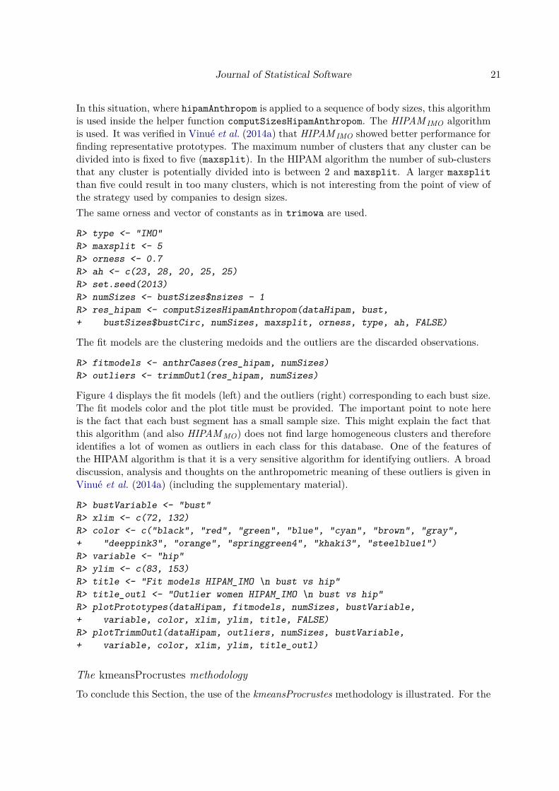
Anthropometry: An R Package for Analysis ofAnthropometric Data
Guillermo VinuéUniversity of Valencia
Abstract
The development of powerful new 3D scanning techniques has enabled the generation oflarge up-to-date anthropometric databases which provide highly valued data to improvethe ergonomic design of products adapted to the user population. As a consequence,Ergonomics and Anthropometry are two increasingly quantitative fields, so advanced sta-tistical methodologies and modern software tools are required to get the maximum benefitfrom anthropometric data.
This paper presents a new R package, called Anthropometry, which is available onthe Comprehensive R Archive Network. It brings together some statistical methodolo-gies concerning clustering, statistical shape analysis, statistical archetypal analysis andthe statistical concept of data depth, which have been especially developed to deal withanthropometric data. They are proposed with the aim of providing effective solutionsto some common anthropometric problems, such as clothing design or workstation de-sign (focusing on the particular case of aircraft cockpits). The utility of the package isshown by analyzing the anthropometric data obtained from a survey of the Spanish femalepopulation performed in 2006 and from the 1967 United States Air Force survey.
This manuscript is also contained in Anthropometry as a vignette.
Keywords: R, anthropometric data, clustering, statistical shape analysis, archetypal analysis,data depth.
1. Introduction
Ergonomics is the science that investigates the interactions between human beings and theelements of a system. The application of ergonomic knowledge in multiple areas such as cloth-ing and footwear design or both working and household environments is required to achievethe best possible match between the product and its users. To that end, it is fundamentalto know the anthropometric dimensions of the target population. Anthropometry refers to
2 Anthropometry: Analysis of Anthropometric Data in R
the study of the measurements and dimensions of the human body and is considered a veryimportant branch of Ergonomics because of its significant influence on the ergonomic designof products (Pheasant 2003).A major issue when developing new patterns and products that fit the target population well isthe lack of up-to-date anthropometric data. Improvements in health care, nutrition and livingconditions as well as the transition to a sedentary life style have changed the body dimensionsof people over recent decades. Anthropometric databases must therefore be updated regularly.Traditionally, human physical characteristics and measurements have been manually takenusing rudimentary methods like calipers, rulers or measuring tapes (Simmons and Istook 2003;Lu and Wang 2008; Shu, Wuhrer, and Xi 2011). These procedures are simple (user-friendly),non-invasive and not particularly expensive. However, obtaining a statistically useful sampleof thousands of people by hand is time-consuming and error-prone: the set of measurementsobtained, and therefore the shape information, is usually imprecise and inaccurate.In recent years, the development of new three-dimensional (3D) body scanner measurementsystems has represented a huge step forward in the way anthropometric data are collected andupdated. This technology provides highly detailed, accurate and reproducible anthropometricdata from which 3D shape images of the people being measured can be obtained (Istookand Hwang 2001; Lerch, MacGillivray, and Domina 2007; Wang, Wu, Lin, Yang, and Lu2007; D’Apuzzo 2009). The great potential of 3D body scanning techniques constitutes atrue breakthrough in realistically characterizing people and has made it possible to conductnew large-scale anthropometric surveys in different countries (for instance, in the USA, theUK, France, Germany and Australia). Within this context, the Spanish Ministry of Healthsponsored a 3D anthropometric study of the Spanish female population in 2006 (Alemany,González, Nácher, Soriano, Arnáiz, and Heras 2010). A sample of 10,415 Spanish females from12 to 70 years old, randomly selected from the official Postcode Address File, was measured.Associated software provided by the scanner manufacturers made a triangulation based onthe 3D spatial location of a large number of points on the body surface. A 3D binary image ofthe trunk of each woman (white pixel if it belongs to the body, otherwise black) is producedfrom the collection of points located on the surface of each woman scanned, as explainedin Ibáñez et al. (2012a). The two main goals of this study, which was conducted by theBiomechanics Institute of Valencia, were as follows: firstly, to characterize the morphology offemales in Spain in order to develop a standard sizing system for the garment industry and,secondly, to encourage an image of healthy beauty in society by means of mannequins thatare representative of the population. In order to tackle both these objectives, Statistics playsan essential role.In every methodological and practical anthropometric problem, body size variability withinthe user population is characterized by means of a limited number of anthropometric cases.This is what is called a user-centered design process. An anthropometric case represents theset of body measurements the product evaluator plans to accommodate in design (HFES 300Committee 2004). A case may be a particular human being or a combination of measurements.Depending on the features and needs of the product being designed, three types of cases can bedistinguished: central, boundary and distributed. If the product being designed is a one-sizeproduct (one-size to accommodate people within a predetermined portion of the population),as may be the case in working environment design, the cases are selected on an accommodationboundary. However, if we focus on a multiple-size product (n sizes to fit n groups of peoplewithin a predetermined portion of the population), clothing design being the most apparent
Journal of Statistical Software 3
example, central cases are selected. Regarding distributed cases, they are spread throughoutthe distribution of body dimensions. Central and boundary cases can be considered specialtypes of distributed cases, but distributed cases might not include them. Distributed casesrepresent an alternative when it is necessary to have a greater number of cases that covers theentire distribution. In such a situation, a small number of central (or boundary) cases wouldnot be sufficient, since they are only spread toward the middle (or edges) of the distribution.The statistical methodologies that we have developed seek to define central and boundarycases to tackle the clothing sizing system design problem and the workplace design problem(focusing on the particular case of an aircraft cockpit).
Clothing sizing systems divide a population into homogeneous subgroups based on some keyanthropometric dimensions (size groups), in such a way that all individuals in a size groupcan wear the same garment (Ashdown 2007; Chung, Lin, and Wang 2007). An efficient andoptimal sizing system must accommodate as large a percentage of the population as possible,in as few sizes as possible, that best describes the shape variability of the population. Inaddition, the garment fit for accommodated individuals must be as good as possible. Eachclothing size is defined from a person who is near the center for the dimensions consideredin the analysis. This central individual, which is considered as the size representative (thesize prototype), becomes the basic pattern from which the clothing line in the same sizeis designed. Once a particular garment has been designed, fashion designers and clothingmanufacturers hire fit models to test and assess the size specifications of their clothing beforethe production phase. Fit models have the appropriate body dimensions selected by eachcompany to define the proportional relationships needed to achieve the fit the company hasdetermined (Loker and Ashdown 2005; Workman and Lentz 2000; Workman 1991). Fit modelsare usually people with central measurements in each body dimension. The definition of anefficient sizing system depends to a large extent on the accuracy and representativeness ofthe fit models.
Clustering is the statistical tool that classifies a set of individuals into groups (clusters), in sucha way that subjects in the same cluster are more similar (in some way) to each other than tothose in other clusters (Kaufman and Rousseeuw 1990). In addition, clusters are representedby means of a representative central observation. Therefore, clustering comes up naturally asa useful statistical approach to try to define an efficient sizing system and to elicit prototypesand fit models. Specifically, five of the methodologies that we have developed are based on dif-ferent clustering methods. Four of them are aimed at segmenting the population into optimalsize groups and obtaining size prototypes. The first one, hereafter referred to as trimowa, hasbeen published in Ibáñez et al. (2012b). It is based on using a special distance function thatmathematically captures the idea of garment fit. The second and third ones (called CCbiclus-tAnthropo and TDDclust) belong to a technical report (Vinué and Ibáñez 2014), which canbe accessed on the author’s website, http://www.uv.es/vivigui/docs/biclustDepth.pdf.The CCbiclustAnthropo methodology adapts a particular clustering algorithm mostly used forthe analysis of gene expression data to the field of Anthropometry. TDDclust uses the statis-tical concept of data depth (Liu, Parelius, and Singh 1999) to group observations accordingto the most central (deep) one in each cluster. As mentioned, traditional sizing systems arebased on using a suitable set of key body dimensions, so clustering must be carried out inthe Euclidean space. In the three previous procedures, we have always worked in this way.Instead, in the fourth and last one, hereinafter called as kmeansProcrustes, a clustering pro-cedure is developed for grouping women according to their 3D body shape, represented by a

4 Anthropometry: Analysis of Anthropometric Data in R
configuration matrix of anatomical markers (landmarks). To that end, the statistical shapeanalysis (Dryden and Mardia 1998) will be fundamental. This approach has been publishedin Vinué, Simó, and Alemany (2014b). Lastly, the fifth clustering proposal is presented withthe goal of identifying accurate fit models and is again used in the Euclidean space. It isbased on another clustering method originally developed for biological data analysis. Thismethod, called hipamAnthropom, has been published in Vinué, León, Alemany, and Ayala(2014a). Well-defined fit models and prototypes can be used to develop representative andprecise mannequins of the population.A sizing system is intended only to cover what is known as the “standard” population, leavingout the individuals who might be considered outliers with respect to a set of measurements. Inthis case, outliers are called disaccommodated individuals. Clothing industries usually designgarments for the standard sizes in order to optimize market share. The four aforementionedmethods concerned with apparel sizing system design (trimowa, CCbiclustAnthropo, TDDclustand kmeansProcrustes) take into account this fact. In addition, because hipamAnthropom isbased on hierarchical features, it is capable of discovering and returning true outliers.Unlike clothing design, where representative cases correspond to central individuals, in de-signing a one-size product, such as working environments or the passenger compartment ofany vehicle, including aircraft cockpits, the most common approach is to search for boundarycases. In these situations, the variability of human shape is described by extreme individuals,which are those that have the smallest or largest values (or extreme combinations) in thedimensions considered in the study. These design problems fall into a more general category:the accommodation problem. The supposition is that the accommodation of boundaries willfacilitate the accommodation of interior points (with less-extreme dimensions) (Bertilsson,Högberg, and Hanson 2012; Parkinson, Reed, Kokkolaras, and Papalambros 2006; HFES 300Committee 2004). For instance, a garage entrance must be designed for a maximum case,while for reaching things such as a brake pedal, the individual minimum must be obtained.In order to tackle the accommodation problem, two methodological contributions based onstatistical archetypal analysis are put forward. An archetype in Statistics is an extreme ob-servation that is obtained as a convex combination of other subjects of the sample (Cutlerand Breiman 1994). The first of these methodologies has been published in Epifanio, Vinué,and Alemany (2013), and the second has been published in Vinué, Epifanio, and Alemany(2015), which presents the new concept of archetypoids.As far as we know, there is currently no reference in the literature related on Anthropometryor Ergonomics that provides the programming of the proposed algorithms. In addition, tothe best of our knowledge, with the exception of modern human modelling tools like “Jack”and “Ramsis”, which are two of the most widely used tools by a broad range of industries(Blanchonette 2010), there are no other general software applications or statistical packagesavailable on the Internet to tackle the definition of an efficient sizing system or the accom-modation problem. Within this context, this paper introduces a new R package (R CoreTeam 2017) called Anthropometry, which brings together the algorithms associated with allthe above-mentioned methodologies. All of them were applied to the anthropometric studyof the Spanish female population and to the 1967 United States Air Force (USAF) survey.Anthropometry includes several data files related to both anthropometric databases. All thestatistical methodologies, anthropometric databases and this R package were announced inthe author’s PhD thesis (Vinué 2014), which is freely available in a Spanish institutional openarchive. The latest version of Anthropometry is always available from the Comprehensive R
Journal of Statistical Software 5
Archive Network at https://CRAN.R-project.org/package=Anthropometry. The packageversion 1.7 (or greater) is needed to reproduce the examples of this manuscript.The outline of the paper is as follows: Section 2 describes all the data files included inAnthropometry. Section 3 is intended to guide users in their choice of the different methodspresented. Section 4 gives a brief explanation of each statistical technique developed. InSection 5 some examples of their application are shown, pointing out at the same time theconsequences of choosing different argument values. Section 6 provides a discussion aboutthe practical usefulness of the methods. Finally, concluding remarks are given in Section 7.One appendix describes the algorithms listings related to each methodology.
2. Data
2.1. Spanish anthropometric survey
The Spanish National Institute of Consumer Affairs (INC according to its Spanish acronym),under the Spanish Ministry of Health and Consumer Affairs, commissioned a 3D anthro-pometric study of the Spanish female population in 2006, after signing a commitment withthe top Spanish companies in the apparel industry. The Spanish National Research Council(CSIC in Spanish) planned and developed the design of the experiment and received advice onAnthropometry from the Complutense University of Madrid. The study itself was conductedby the Biomechanics Institute of Valencia (Alemany et al. 2010). The target sample wasmade up of 10,415 women grouped into 10 age groups ranging from 12 to 70 years, randomlychosen from the official Postcode Address File.As an illustrative example of the full Spanish survey, Anthropometry contains a databasecalled sampleSpanishSurvey, made up of a sample of 600 Spanish women and their measure-ments for five anthropometric variables: bust, chest, waist and hip circumferences and neck toground length. These variables are chosen for three main reasons: they are recommended byexperts, they are commonly used in the literature and they appear in the European standardon sizing systems. Size designation of clothes. Part 2: Primary and secondary dimensions(European Committee for Standardization 2002).As mentioned above, the women’s shape is represented by a set of landmarks, specifically66 points. A data file called landmarksSampleSpaSurv contains the configuration matrixof landmarks for each of the 600 women. As also noted above, a 3D binary image of eachwoman’s trunk is available. Hence, the dissimilarity between trunk forms can be computedand a distance matrix between women can be built. The distance matrix used in Vinué et al.(2015) is included in Anthropometry and is called descrDissTrunks.
2.2. USAF survey
This database contains the information provided by the 1967 United States Air Force (USAF)survey. It can be downloaded from http://www.dtic.mil/dtic/. This survey was conductedin 1967 by the anthropology branch of the Aerospace Medical Research Laboratory (Ohio).A sample of 2420 subjects of the Air Force personnel, between 21 and 50 years of age, weremeasured at 17 Air Force bases across the United States of America. A total of 202 variableswere collected. The dataset associated with the USAF survey is available on USAFSurvey. In
6 Anthropometry: Analysis of Anthropometric Data in R
the methodologies related to archetypal analysis, six anthropometric variables from the totalof 202 will be selected. They are the same as those selected in Zehner, Meindl, and Hudson(1993) and are called cockpit dimensions because they are critical in order for designing anaircraft cockpit.
2.3. Geometric figures
Two geometric figures, a cube and a parallelepiped, made up of 8 and 34 landmarks, areavailable in the package as cube8landm, cube34landm, parallelep8landm andparallelep34landm, respectively.
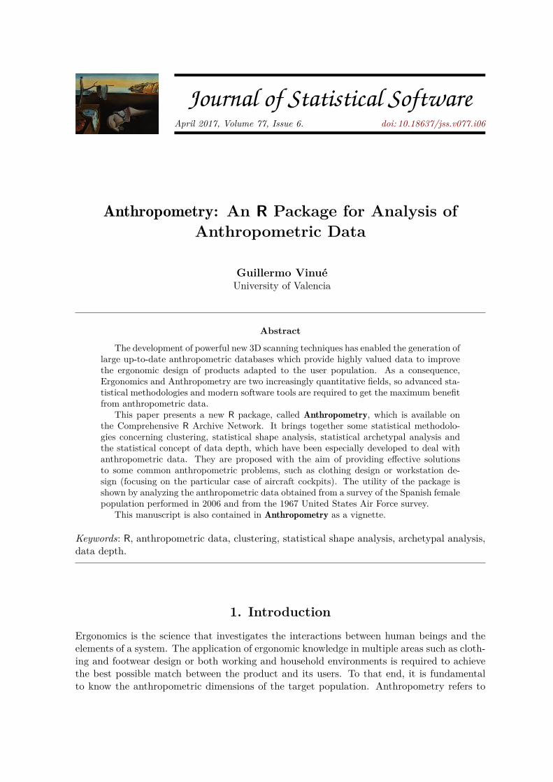
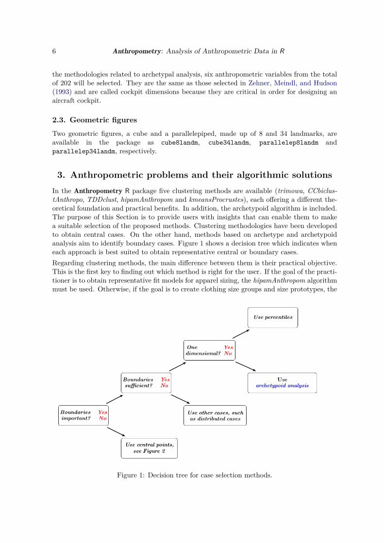
3. Anthropometric problems and their algorithmic solutionsIn the Anthropometry R package five clustering methods are available (trimowa, CCbiclus-tAnthropo, TDDclust, hipamAnthropom and kmeansProcrustes), each offering a different the-oretical foundation and practical benefits. In addition, the archetypoid algorithm is included.The purpose of this Section is to provide users with insights that can enable them to makea suitable selection of the proposed methods. Clustering methodologies have been developedto obtain central cases. On the other hand, methods based on archetype and archetypoidanalysis aim to identify boundary cases. Figure 1 shows a decision tree which indicates wheneach approach is best suited to obtain representative central or boundary cases.Regarding clustering methods, the main difference between them is their practical objective.This is the first key to finding out which method is right for the user. If the goal of the practi-tioner is to obtain representative fit models for apparel sizing, the hipamAnthropom algorithmmust be used. Otherwise, if the goal is to create clothing size groups and size prototypes, the
Figure 1: Decision tree for case selection methods.

Journal of Statistical Software 7
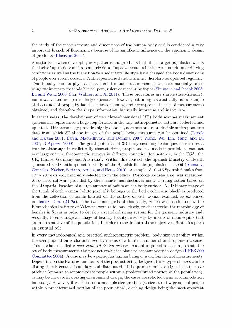
Figure 2: Decision tree as user guidance for choosing which of the different clustering methodsto apply.
other four methods are suitable. If the user wanted to design lower body garments, CCbiclus-tAnthropo should be chosen, while for designing upper body garments, trimowa, TDDclustand kmeansProcrustes are suitable. Choosing one of the latter three methods depends on thekind of data being collected. If the database contains a set of 3D landmarks representing theshape of women, the kmeansProcrustes method must be applied. On the other hand, trimowaand TDDclust can be used when the data are 1D body measurements. For illustrative pur-poses, Figure 2 shows a decision tree that helps the user to decide which clustering approachis best suited.As a conclusion to this discussion, an illustrative comparison of the outcomes of using trimowaand TDDclust on a random sample subset is given below. We restrict our attention to thesetwo methods because both of them have the same intention. Table 1 shows, in blue and witha frame box, the upper prototypes obtained with TDDclust and with trimowa, respectively(the R code used to obtain these results is available in the supplementary file v77i06.R). Inthis case, two of the three prototypes match. However, it is worth pointing out that in anothercase it is possible that none of them would match. This is because of the different statisticalfoundation of each approach. At this point, it would be recommendable to use the trimowamethodology because it has been developed further than TDDclust, returns outcomes witha significantly lower computational time, regardless of the sample size, and is endorsed by ascientific publication.
4. Statistical methodologies
4.1. Anthropometric dimensions-based clustering and shape analysis
For practical guidance, Algorithm 1 explains the workflow for clustering-based approaches

8 Anthropometry: Analysis of Anthropometric Data in R
Label women neck to ground waist bust92 134.3 71.1 82.7480 133.1 96.8 106.5340 136.3 85.9 95.9377 136.1 87.6 97.9
Table 1: Upper size prototypes obtained by TDDclust (in italics) and by trimowa (framebox).
Algorithm 1 Workflow for clustering-based approaches.1. The data matrix is segmented using a primary control dimension (bust or waist).Note 1: The segmentation is done according to the classes suggested in the Europeanstandard on sizing systems. Size designation of clothes. Part 3: Measurementsand intervals (European Committee for Standardization 2005). This standardis drawn up by the European Union and is a set of guidelines for the textileindustry to promote the implementation of a clothing sizing system, that isadapted to users.
2. A further clustering segmentation is carried out using other secondary control anthropometricvariables.if bust was selected in 1. then
use one of the following methodologies:- trimowa (see Algorithm 3).- TDDclust (see Algorithm 5).- hipamAnthropom (see Algorithm 6).- kmeansProcrustes (see Algorithm 9, 10 and 11).
elseif waist was selected in 1. then
use CCbiclustAnthropo (see Algorithm 4).end if
end ifNote 2: In this way, the first segmentation provides a first easy input to choose thesize, while the resulting clusters (subgroups) for each bust (or waist) and otheranthropometric measurements optimize the sizing. From the point of view ofclothing design, by using a more appropriate statistical strategy, such asclustering, homogeneous subgroups are generated taking into account theanthropometric variability of the secondary dimensions that have a significantinfluence on garment fit.
from an Anthropometry point of view, followed by the description of individual algorithms.See Appendix A for details about the algorithm listings.
The trimowa methodology
The aim of a sizing system is to divide a varied population into groups using certain keybody dimensions (Ashdown 2007; Chung et al. 2007). Three types of approaches can bedistinguished for creating a sizing system: traditional step-wise sizing, multivariate methodsand optimization methods. Traditional methods are not useful because they use bivariatedistributions to define a sizing chart and do not consider the variability of other relevantanthropometric dimensions. Recently, more sophisticated statistical methods have been de-
Journal of Statistical Software 9
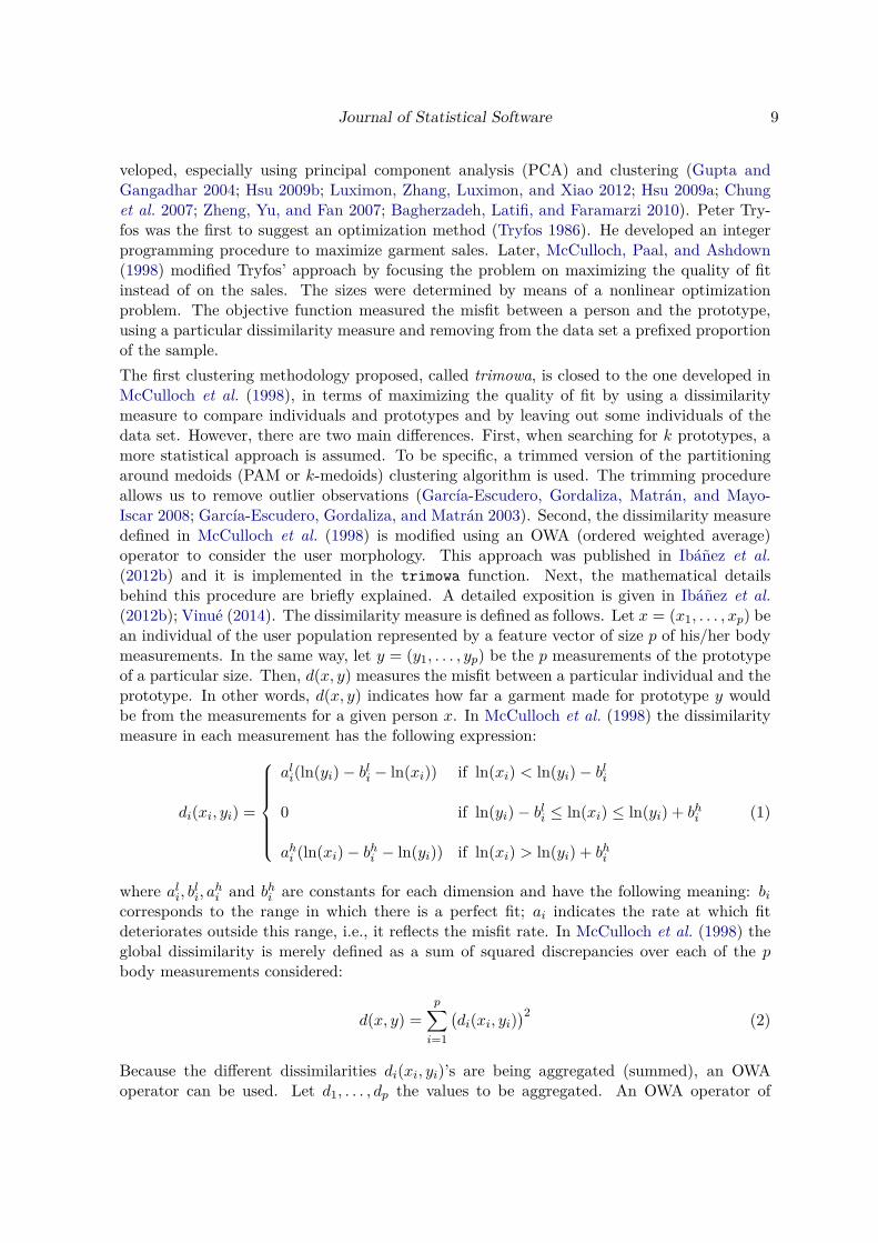
veloped, especially using principal component analysis (PCA) and clustering (Gupta andGangadhar 2004; Hsu 2009b; Luximon, Zhang, Luximon, and Xiao 2012; Hsu 2009a; Chunget al. 2007; Zheng, Yu, and Fan 2007; Bagherzadeh, Latifi, and Faramarzi 2010). Peter Try-fos was the first to suggest an optimization method (Tryfos 1986). He developed an integerprogramming procedure to maximize garment sales. Later, McCulloch, Paal, and Ashdown(1998) modified Tryfos’ approach by focusing the problem on maximizing the quality of fitinstead of on the sales. The sizes were determined by means of a nonlinear optimizationproblem. The objective function measured the misfit between a person and the prototype,using a particular dissimilarity measure and removing from the data set a prefixed proportionof the sample.The first clustering methodology proposed, called trimowa, is closed to the one developed inMcCulloch et al. (1998), in terms of maximizing the quality of fit by using a dissimilaritymeasure to compare individuals and prototypes and by leaving out some individuals of thedata set. However, there are two main differences. First, when searching for k prototypes, amore statistical approach is assumed. To be specific, a trimmed version of the partitioningaround medoids (PAM or k-medoids) clustering algorithm is used. The trimming procedureallows us to remove outlier observations (García-Escudero, Gordaliza, Matrán, and Mayo-Iscar 2008; García-Escudero, Gordaliza, and Matrán 2003). Second, the dissimilarity measuredefined in McCulloch et al. (1998) is modified using an OWA (ordered weighted average)operator to consider the user morphology. This approach was published in Ibáñez et al.(2012b) and it is implemented in the trimowa function. Next, the mathematical detailsbehind this procedure are briefly explained. A detailed exposition is given in Ibáñez et al.(2012b); Vinué (2014). The dissimilarity measure is defined as follows. Let x = (x1, . . . , xp) bean individual of the user population represented by a feature vector of size p of his/her bodymeasurements. In the same way, let y = (y1, . . . , yp) be the p measurements of the prototypeof a particular size. Then, d(x, y) measures the misfit between a particular individual and theprototype. In other words, d(x, y) indicates how far a garment made for prototype y wouldbe from the measurements for a given person x. In McCulloch et al. (1998) the dissimilaritymeasure in each measurement has the following expression:
di(xi, yi) =
ali(ln(yi)− bli − ln(xi)) if ln(xi) < ln(yi)− bli
0 if ln(yi)− bli ≤ ln(xi) ≤ ln(yi) + bhi
ahi (ln(xi)− bhi − ln(yi)) if ln(xi) > ln(yi) + bhi
(1)
where ali, bli, ahi and bhi are constants for each dimension and have the following meaning: bicorresponds to the range in which there is a perfect fit; ai indicates the rate at which fitdeteriorates outside this range, i.e., it reflects the misfit rate. In McCulloch et al. (1998) theglobal dissimilarity is merely defined as a sum of squared discrepancies over each of the pbody measurements considered:
d(x, y) =p∑i=1
(di(xi, yi)
)2 (2)
Because the different dissimilarities di(xi, yi)’s are being aggregated (summed), an OWAoperator can be used. Let d1, . . . , dp the values to be aggregated. An OWA operator of
10 Anthropometry: Analysis of Anthropometric Data in R
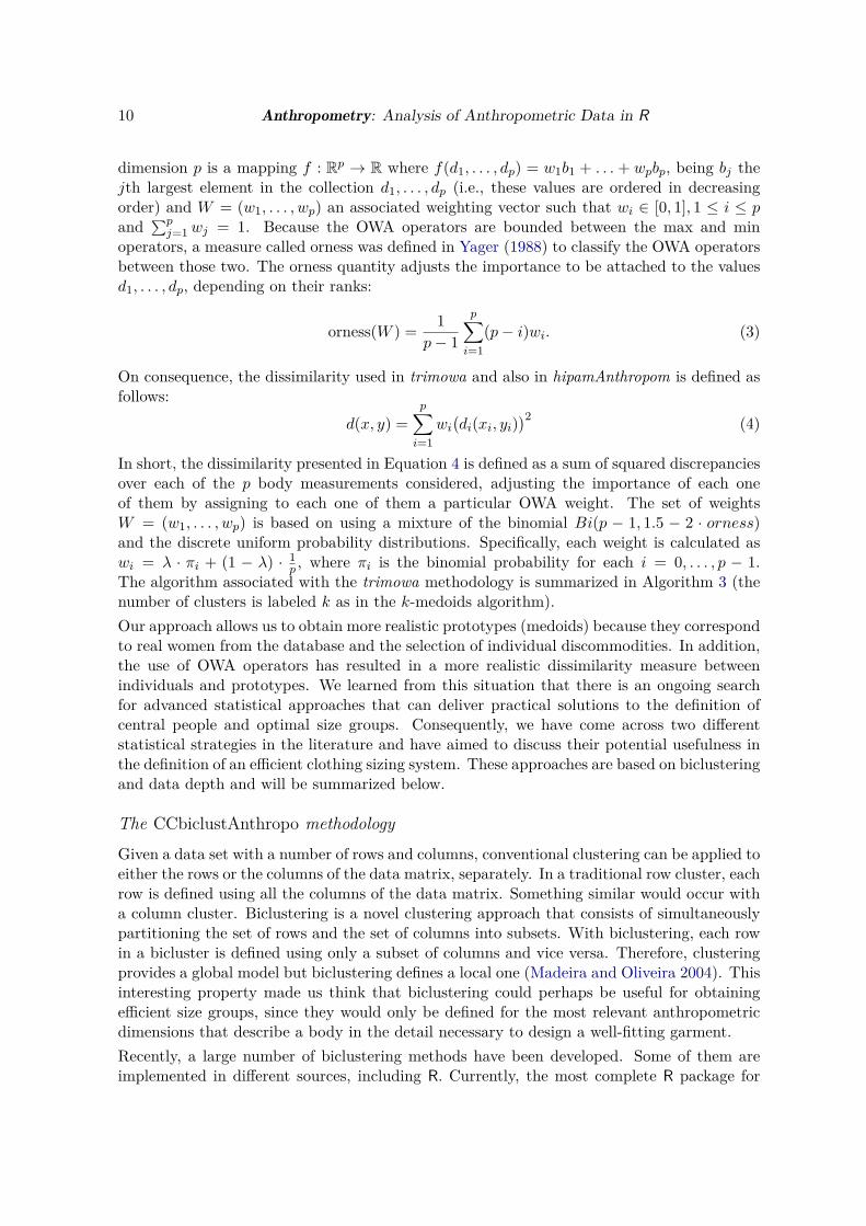
dimension p is a mapping f : Rp → R where f(d1, . . . , dp) = w1b1 + . . . + wpbp, being bj thejth largest element in the collection d1, . . . , dp (i.e., these values are ordered in decreasingorder) and W = (w1, . . . , wp) an associated weighting vector such that wi ∈ [0, 1], 1 ≤ i ≤ pand ∑p
j=1wj = 1. Because the OWA operators are bounded between the max and minoperators, a measure called orness was defined in Yager (1988) to classify the OWA operatorsbetween those two. The orness quantity adjusts the importance to be attached to the valuesd1, . . . , dp, depending on their ranks:
orness(W ) = 1p− 1
p∑i=1
(p− i)wi. (3)
On consequence, the dissimilarity used in trimowa and also in hipamAnthropom is defined asfollows:
d(x, y) =p∑i=1
wi(di(xi, yi)
)2 (4)
In short, the dissimilarity presented in Equation 4 is defined as a sum of squared discrepanciesover each of the p body measurements considered, adjusting the importance of each oneof them by assigning to each one of them a particular OWA weight. The set of weightsW = (w1, . . . , wp) is based on using a mixture of the binomial Bi(p − 1, 1.5 − 2 · orness)and the discrete uniform probability distributions. Specifically, each weight is calculated aswi = λ · πi + (1 − λ) · 1
p , where πi is the binomial probability for each i = 0, . . . , p − 1.The algorithm associated with the trimowa methodology is summarized in Algorithm 3 (thenumber of clusters is labeled k as in the k-medoids algorithm).Our approach allows us to obtain more realistic prototypes (medoids) because they correspondto real women from the database and the selection of individual discommodities. In addition,the use of OWA operators has resulted in a more realistic dissimilarity measure betweenindividuals and prototypes. We learned from this situation that there is an ongoing searchfor advanced statistical approaches that can deliver practical solutions to the definition ofcentral people and optimal size groups. Consequently, we have come across two differentstatistical strategies in the literature and have aimed to discuss their potential usefulness inthe definition of an efficient clothing sizing system. These approaches are based on biclusteringand data depth and will be summarized below.
The CCbiclustAnthropo methodology
Given a data set with a number of rows and columns, conventional clustering can be applied toeither the rows or the columns of the data matrix, separately. In a traditional row cluster, eachrow is defined using all the columns of the data matrix. Something similar would occur witha column cluster. Biclustering is a novel clustering approach that consists of simultaneouslypartitioning the set of rows and the set of columns into subsets. With biclustering, each rowin a bicluster is defined using only a subset of columns and vice versa. Therefore, clusteringprovides a global model but biclustering defines a local one (Madeira and Oliveira 2004). Thisinteresting property made us think that biclustering could perhaps be useful for obtainingefficient size groups, since they would only be defined for the most relevant anthropometricdimensions that describe a body in the detail necessary to design a well-fitting garment.Recently, a large number of biclustering methods have been developed. Some of them areimplemented in different sources, including R. Currently, the most complete R package for

Journal of Statistical Software 11
biclustering is biclust (Kaiser and Leisch 2008; Kaiser et al. 2015). The usefulness of the ap-proaches included in biclust for dealing with anthropometric data was investigated in Vinué(2012). Among the conclusions reached, the most important was concerned with the possi-bility of considering the Cheng & Church biclustering algorithm (Cheng and Church 2000)(referred to below as CC) as a potential statistical approach to be used for defining sizegroups. Specifically, in Vinué (2012) an algorithm to find size groups (biclusters) and dis-accommodated women with CC was set out. This methodology is called CCbiclustAnthropoand it is implemented in the CCbiclustAnthropo function. Next, the mathematical detailsbehind the CCbiclustAnthropo procedure are briefly described. First of all, the CC algorithmmust be introduced (see Cheng and Church 2000; Vinué 2014; Kaiser and Leisch 2008, formore details). The CC algorithm searches for biclusters with constant values (in rows or incolumns). To that end, it defines the following score:
H(I, J) = 1|I||J |
∑i∈I,j∈J
(aij − aiJ − aIj + aIJ)2,
where aiJ is the mean of the ith row of the bicluster, aIj is the mean of the jth column ofthe bicluster and aIJ is its overall mean. Then, a subgroup is called a bicluster if the score isbelow a value δ ≥ 0 and above an α-fraction of the score of the whole data (α > 1).The CC algorithm implemented in the biclust function of the biclust package requires threearguments. Firstly, the maximum number of biclusters to be found. We propose that thisnumber should be fixed for each waist size according to the number of women it contains:For less than 150, fix 2 biclusters; between 151-300, 3; between 351-450, 4; greater than 415,5. Secondly, the α value. Its default value (1.5) is maintained. Finally, the δ value. BecauseCC is nonexhaustive, i.e., it might not group every woman into a bicluster, the value of δcan be iteratively adapted to the number of disaccommodated women we want to discard ineach size. The proportion of the trimmed sample is prefixed to 0.01 per size. In this way, anumber of women between 0 and the previous fixed proportion will not be assigned to anygroup. The algorithm associated with the CCbiclustAnthropo methodology is summarized inAlgorithm 4.Designing lower body garments depends not only on the waist circumference (the principaldimension in this case), but also on other secondary control dimensions (for upper body gar-ments only the bust circumference is usually needed). Biclustering produces subgroups ofobjects that are similar in one subgroup of variables and different in the remaining variables.Therefore, it seems more interesting to use a biclustering algorithm with a set of lower bodydimensions. For that purpose, all the body variables related to the lower body in the Spanishanthropometric survey were chosen (there were 36). An efficient partition into different bi-clusters was obtained with promising results. All individuals in the same bicluster can weara garment designed for the specific body dimensions (waist and other variables) which werethe most relevant for defining the group. Each group is represented by the median woman.The main interest of this approach was descriptive and exploratory and the important pointto note here is that CCbiclustAnthropo cannot be used with sampleSpanishSurvey, sincethis data file does not contain variables related to the lower body in addition to waist andhip. However, this function is included in the package in the hope that it could be helpfulor useful for other researchers. All theoretical and practical details are given in Vinué andIbáñez (2014), Vinué (2014) and Vinué (2012).

12 Anthropometry: Analysis of Anthropometric Data in R
The TDDclust methodologyThe statistical concept of data depth is another general framework for descriptive and infer-ential analysis of numerical data in a certain number of dimensions. In essence, the notionof data depth is a generalization of standard univariate rank methods in higher dimensions.A depth function measures the degree of centrality of a point regarding a probability distri-bution or a data set. The highest depth values correspond to central points and the lowestdepth values correspond to tail points (Liu et al. 1999; Zuo and Serfling 2000). Therefore,the depth paradigm is another very interesting strategy for identifying central prototypes.The development of clustering and classification methods using data depth measures hasreceived increasing attention in recent years (Dutta and Ghosh 2012; Lange, Mosler, andMozharovskyi 2012; Romo and López 2010; Ding, Dang, Peng, and Wilkins 2007). The mostrelevant contribution to this field has been made by Rebecka Jörnsten in Jörnsten (2004)(see Jörnsten, Vardi, and Zhang 2002; Pan, Jörnsten, and Hart 2004, for more details). Sheintroduced two clustering and classification methods (DDclust and DDclass, respectively)based on L1 data depth (see Vardi and Zhang 2000, for more details). The DDclust methodis proposed to solve the problem of minimizing the sum of L1-distances from the observationsto the nearest cluster representatives. In clustering terms, the L1 data depth is the amountof probability mass needed at a point z to make z the multivariate L1-median (a robustrepresentative) of the data cluster.An extension of DDclust is introduced which incorporates a trimmed procedure, aimed at seg-menting the data into efficient size groups using central (the deepest) people. This method-ology will be referred to below as TDDclust and it can be used within Anthropometry byusing a function with the same name. Next, the mathematical details behind the TDDclustprocedure are briefly described. A thorough explanation is given in Vinué and Ibáñez (2014);Vinué (2014). First, the L1 multivariate median (from now on, L1-MM) is defined as thesolution of the Weiszfeld problem (Vardi and Zhang 2000). Vardi and Zhang (2000) provedthat the depth function associated with the L1-MM, called L1 data depth, is:
D(y) =
1− ||e(y)|| if y /∈ {x1, . . . , xm},
1− (||e(y)|| − fk) if y = xk.(5)
where ei(y) = (y− xi)/||y− xi|| (unit vector from y to xi) and e(y) = ∑xk 6=y ei(y)fi (average
of the unit vectors from y to all observations), with fi = ηi /∑kj=1 ηj (ηi is a weight for xi)
and ||e(y)|| is close to 1 if y is close to the edge of the data, and close to 0 if y is close to thecenter.The DDclust method is proposed to solve the problem of minimizing the sum of L1-distancesfrom the observations to the nearest cluster representatives. Specifically, DDclust iteratesbetween median computations via the modified Weiszfeld algorithm (Weiszfeld and Plastria2009) and a Nearest-Neighbor allocation scheme with simulation annealing. The clusteringcriterion function used in DDclust is the maximization of:
C(IK1 ) = 1N
K∑k=1
∑i∈I(k)
(1− λ)sili + λReDi (6)
with respect to a partition IK1 = {I(1), . . . , I(K)}. For each point i, sili is the silhouettewidth, ReDi is the difference between the within cluster L1 data depth and the between
Journal of Statistical Software 13
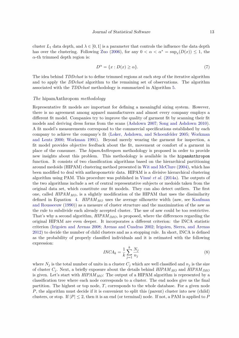
cluster L1 data depth, and λ ∈ [0, 1] is a parameter that controls the influence the data depthhas over the clustering. Following Zuo (2006), for any 0 < α < α∗ = supx(D(x)) ≤ 1, theα-th trimmed depth region is:
Dα = {x : D(x) ≥ α}. (7)
The idea behind TDDclust is to define trimmed regions at each step of the iterative algorithmand to apply the DDclust algorithm to the remaining set of observations. The algorithmassociated with the TDDclust methodology is summarized in Algorithm 5.
The hipamAnthropom methodology
Representative fit models are important for defining a meaningful sizing system. However,there is no agreement among apparel manufacturers and almost every company employs adifferent fit model. Companies try to improve the quality of garment fit by scanning their fitmodels and deriving dress forms from the scans (Ashdown 2007; Song and Ashdown 2010).A fit model’s measurements correspond to the commercial specifications established by eachcompany to achieve the company’s fit (Loker, Ashdown, and Schoenfelder 2005; Workmanand Lentz 2000; Workman 1991). Beyond merely wearing the garment for inspection, afit model provides objective feedback about the fit, movement or comfort of a garment inplace of the consumer. The hipamAnthropom methodology is proposed in order to providenew insights about this problem. This methodology is available in the hipamAnthropomfunction. It consists of two classification algorithms based on the hierarchical partitioningaround medoids (HIPAM) clustering method presented in Wit and McClure (2004), which hasbeen modified to deal with anthropometric data. HIPAM is a divisive hierarchical clusteringalgorithm using PAM. This procedure was published in Vinué et al. (2014a). The outputs ofthe two algorithms include a set of central representative subjects or medoids taken from theoriginal data set, which constitute our fit models. They can also detect outliers. The firstone, called HIPAM MO, is a slightly modification of the HIPAM that uses the dissimilaritydefined in Equation 4. HIPAM MO uses the average silhouette width (asw, see Kaufmanand Rousseeuw (1990)) as a measure of cluster structure and the maximization of the asw asthe rule to subdivide each already accepted cluster. The use of asw could be too restrictive.That’s why a second algorithm, HIPAM IMO, is proposed, where the differences regarding theoriginal HIPAM are even deeper. It incorporates a different criterion: the INCA statisticcriterion (Irigoien and Arenas 2008; Arenas and Cuadras 2002; Irigoien, Sierra, and Arenas2012) to decide the number of child clusters and as a stopping rule. In short, INCA is definedas the probability of properly classified individuals and it is estimated with the followingexpression:
INCAk = 1k
k∑j=1
Nj
nj(8)
where Nj is the total number of units in a cluster Cj which are well classified and nj is the sizeof cluster Cj . Next, a briefly exposure about the details behind HIPAM MO and HIPAM IMOis given. Let’s start with HIPAM MO: The output of a HIPAM algorithm is represented by aclassification tree where each node corresponds to a cluster. The end nodes give us the finalpartition. The highest or top node, T , corresponds to the whole database. For a given nodeP , the algorithm must decide if it is convenient to split this (parent) cluster into new (child)clusters, or stop. If |P | ≤ 2, then it is an end (or terminal) node. If not, a PAM is applied to P

14 Anthropometry: Analysis of Anthropometric Data in R
with k1 groups, where k1 is chosen by maximizing the asw of the new partition. After a post-processing step, a partition C = {C1, . . . , Ck} is finally obtained from P (k is not necessarilyequal to k1). Next, the mean silhouette width of C (or aswC) is obtained, and then the samesteps used to generate C are applied to each Ci to obtain a new partition. If we denote by SSithe asw of the new partition with i = 1, . . . , k (if |Ci| ≤ 2 then SSi = 0), then the mean splitsilhouette (MSS) is defined as the mean of the SSi’s. If MSS(k) < aswC , then these newk child clusters of the partition C are included in the classification tree. Otherwise, P is aterminal node. On the other hand, the algorithm HIPAM IMO is summarized in Algorithm 6.The main difference between HIPAM MO and HIPAM IMO is in the use of the INCA criterion:
1. At each node P , if there is k such that INCAk > 0.2, then we select the k prior to thefirst largest slope decrease.
2. On the other hand, if INCAk < 0.2 for all k, then P is a terminal node.
However, this procedure does not apply either to the top node T , or to the generation of thenew partitions from which the MSS is calculated. In this case, even when all INCAk < 0.2,we fix k = 3 as the number of groups to divide and proceed.
The kmeansProcrustes methodology
The clustering methodologies explained so far use a set of control anthropometric variables asthe basis for a different type of sizing system in which people are grouped in a size group basedon a full range of measurements. Consequently, clustering is done in the Euclidean space.The shape of the women recruited into the Spanish anthropometric survey is representedby a configuration matrix of correspondence points called landmarks. Taking advantage ofthis fact, we have adapted the k-means clustering algorithm to the field of statistical shapeanalysis, to define size groups of women according to their body shapes. The representative ofeach size group is the average woman. This approach was published in Vinué et al. (2014b).We have adapted both the original Lloyd and Hartigan-Wong (H-W) versions of k-meansto the field of shape analysis and we have demonstrated, by means of a simulation study,that the Lloyd version is more efficient for clustering shapes than the H-W version. Thefunction that uses the Lloyd version of k-means adapted to shape analysis (what we calledkmeansProcrustes) is LloydShapes. The function that uses the H-W version of k-meansadapted to shape analysis is HartiganShapes. A trimmed version of kmeansProcrustes canbe also executed with trimmedLloydShapes.To adapt k-means to the context of shape analysis, we integrated the Procrustes distance andProcrustes mean into it. A glossary of the concepts of shape analysis used is provided below.The following general notation will be used: n refers to the number of objects, h to the numberof landmarks and m to the number of dimensions (in our case, m = 3). Then, each objectis described by an h×m configuration matrix X containing the m Cartesian coordinates ofits h landmarks. The pre-shape of an object is what is left after allowing for the effects oftranslation and scale. The shape of an object is what is left after allowing for the effects oftranslation, scale and rotation. The shape space Σh
m (named Kendall shape space) is the set ofall possible shapes. The Procrustes distance is the square root of the sum of squared differencesbetween the positions of the landmarks in two optimally (by least-squares) superimposedconfigurations at centroid size (the centroid size is the most commonly used measure of sizefor a configuration). The Procrustes mean is the shape that has the least summed squared

Journal of Statistical Software 15
Algorithm 2 Workflow for archetypal-based approaches.1. Depending on the problem, the data may or may not be standardized.2. An accommodation subsample is selected.3. A number k of archetypes is obtained (see Algorithm 12).4. The nearest individuals to the archetypes are computed.5. A number k of archetypoids is obtained (see Algorithm 13).
Procrustes distance to all the configurations of a sample. Algorithms 9, 10 and 11 show thealgorithms behind LloydShapes, trimmedLloydShapes and HartiganShapes, respectively.
4.2. Archetypal analysis
Regarding the methodologies using archetypal analysis, for practical guidance, Algorithm 2explains their corresponding workflow, followed by the description of individual algorithms.See Appendix A for details about the algorithm listings.In ergonomic-related problems, where the goal is to create more efficient people-machineinterfaces, a small set of extreme cases (boundary cases), called human models, is sought.Designing for extreme individuals is appropriate where some limiting factor can define eithera minimum or maximum value which will accommodate the population. The basic principle isthat accommodating boundary cases will be sufficient to accommodate the whole population.For too long, the conventional solution for selecting this small group of boundary modelswas based on the use of percentiles. However, percentiles are a kind of univariate descriptivestatistic, so they are suitable only for univariate accommodation and should not be used indesigns that involve two or more dimensions. Furthermore, they are not additive (Zehneret al. 1993; Robinette and McConville 1981; Moroney and Smith 1972). Today, the alterna-tive commonly used for the multivariate accommodation problem is based on PCA (Friessand Bradtmiller 2003; Hudson, Zehner, and Meindl 1998; Robinson, Robinette, and Zehner1992; Bittner, Glenn, Harris, Iavecchia, and Wherry 1987). However, it is known that thePCA approach presents some drawbacks (Friess 2005). In Epifanio et al. (2013), a differentstatistical approach for determining multivariate limits was put forward: archetypal analy-sis (Cutler and Breiman 1994), and its advantages regarding over PCA were demonstrated.The theoretical basis of archetype analysis is as follows. Let X be an n × m matrix thatrepresents a multivariate dataset with n observations and m variables. The goal of archetypeanalysis is to find a k ×m matrix Z that characterizes the archetypal patterns in the data,such that data can be represented as mixtures of those archetypes. Specifically, archetypeanalysis is aimed at obtaining the two n × k coefficient matrices α and β which minimizethe residual sum of squares that arises from combining the equation that shows xi as beingapproximated by a linear combination of zj ’s (archetypes) and the equation that shows zj ’sas linear combinations of the data:
‖xi −∑kj=1 αijzj‖2
zj =n∑l=1
βjlxl
⇒ RSS =n∑i=1‖xi −
k∑j=1
αijzj‖2 =n∑i=1‖xi −
k∑j=1
αij
n∑l=1
βjlxl‖2, (9)
under the constraints
16 Anthropometry: Analysis of Anthropometric Data in R
1)k∑j=1
αij = 1 with αij ≥ 0 and i = 1, . . . , n and
2)n∑l=1
βjl = 1 with βjl ≥ 0 and j = 1, . . . , k.
On the one hand, constraint 1) tells us that the predictors of xi are finite mixtures of
archetypes, xi =k∑j=1
αijzj . Each αij is the weight of the archetype j for the individual i,
that is to say, the α coefficients represent how much each archetype contributes to the ap-proximation of each individual. On the other hand, constraint 2) implies that archetypes zj
are convex combinations of the data points, zj =n∑l=1
βjlxl. Algorithm 12 shows an outline of
the archetypal algorithm, following Eugster and Leisch (2009).The function that allows us to reproduce the results discussed in Epifanio et al. (2013) isarchetypesBoundary (use set.seed(2010) to obtain the same results).According to the previous definition, archetypes computed by archetypal analysis are a convexcombination of the sampled individuals, but they are not necessarily real observations. Thearchetypes would correspond to specific individuals when zj is an observation of the sample,that is to say, when only one βjl is equal to 1 in constraint 2) for each j. As βjl ≥ 0and the sum of constraint 2) is 1, this implies that βjl should only take on the value 0 or1. In some problems, it is crucial that the archetypes are real subjects, observations of thesample, and not fictitious. To that end, we have proposed a new archetypal concept: thearchetypoid, which corresponds to specific individuals and each observation of the data setcan be represented as a mixture of these archetypoids. In the analysis of archetypoids, theoriginal continuous optimization problem therefore becomes:
RSS =n∑i=1‖xi −
k∑j=1
αijzj‖2 =n∑i=1‖xi −
k∑j=1
αij
n∑l=1
βjlxl‖2, (10)
under the constraints
1)k∑j=1
αij = 1 with αij ≥ 0 and i = 1, . . . , n and
2)n∑l=1
βjl = 1 with βjl ∈ {0, 1} and j = 1, . . . , k i.e., βjl = 1 for one and only one l and
βjl = 0 otherwise.
This new concept archetypoids is introduced in a paper published in Vinué et al. (2015). Wehave developed an efficient computational algorithm based on PAM to compute archetypoids(called archetypoid algorithm), we have analyzed some of their theoretical properties, we haveexplained how they can be obtained when only dissimilarities between observations are known(features are unavailable) and we have demonstrated some of their advantages regarding overclassical archetypes.

Journal of Statistical Software 17
The archetypoid algorithm has two phases: a BUILD phase and a SWAP phase, like PAM.In the BUILD step, an initial set of archetypoids is determined, made up of the nearestindividuals to the archetypes computed in the first instance. This set can be defined in threedifferent ways: The first possibility consists in computing the Euclidean distance between thek archetypes and the individuals and choosing the nearest ones, as mentioned in Epifanio et al.(2013) (set candns). The second choice identifies the individuals with the maximum α value foreach archetype, i.e., the individuals with the largest relative share for the respective archetype(set candα, used in Eugster 2012 and Seiler and Wohlrabe 2013). The third choice identifiesthe individuals with the maximum β value for each archetype, i.e., the major contributorsin the generation of the archetypes (set candβ). Accordingly, the initial set of archetypoidsis candns, candα or candβ. The aim of the SWAP phase of the archetypoid algorithm isthe same as that of the SWAP phase of PAM, but the objective function is now given byEquation 10 (see Vinué et al. 2015; Vinué 2014, for more details). Algorithm 13 shows anoutline of the archetypoid algorithm.
5. ApplicationsThis Section presents a detailed explanation of the numerical and graphical outcome providedby each method by means of several examples. In addition, some relevant comments are givenabout the consequences of choosing different argument values in each case.First of all, Anthropometry must be loaded into R:
R> library("Anthropometry")
5.1. Anthropometric dimensions-based clustering and shape analysis
The trimowa methodology
The following code executes the trimowa methodology. A similar code was used to obtainthe results described in Ibáñez et al. (2012b). We use sampleSpanishSurvey and its fiveanthropometric variables. The bust circumference is used as the primary control dimension.Twelve bust sizes (from 74 cm to 131 cm) are defined according to the European standard onsizing systems. Size designation of clothes. Part 3: Measurements and intervals (EuropeanCommittee for Standardization 2005).
R> dataTrimowa <- sampleSpanishSurveyR> numVar <- dim(dataTrimowa)[2]R> bust <- dataTrimowa$bustR> bustSizes <- bustSizesStandard(seq(74, 102, 4), seq(107, 131, 6))
The aggregation weights of the OWA operator are computed. They are used to calculate theglobal dissimilarity between the individuals and the prototypes. We give orness a value of 0.7in order to highlight the largest aggregated values, that is to say, the largest discrepanciesbetween the women’s body measurements and those of the prototype. An orness value closeto 1 gives more importance to the worst fit, whilst an orness value close to 0 gives moreimportance to the best fit (see Vinué 2014, p. 27–31, for details).

18 Anthropometry: Analysis of Anthropometric Data in R
R> orness <- 0.7R> weightsTrimowa <- weightsMixtureUB(orness, numVar)
Next the trimowa algorithm is used within each bust size. In this situation, where trimowais applied to a sequence of body sizes, this algorithm is used inside the helper functioncomputSizesTrimowa. Three size groups (clusters, argument numClust) are calculated perbust segment. This number of groups is quite well aligned with the strategy used by companiesto design sizes. A larger numClust will result in many sizes being designed, increasing theproduction a lot. A smaller numClust corresponds to too few sizes being designed and havinga poor accommodation index.The trimmed proportion, alpha, is prefixed to 0.01 per segment (therefore, the accommo-dation rate in each bust size will be 99%). This selection allows us to accommodate a verylarge percentage of the population in the sizing system. A larger trimmed proportion wouldresult in a smaller amount of accommodated people. The number of random initializationsis 10 (niter), with seven steps per initialization (algSteps). These values are small in theinterests of a fast execution. The more random repetitions, the more accurate the prototypesand the more representative of the size group. In Ibáñez et al. (2012b), the number of randominitializations was 600.In addition, a vector of five constants (one per variable) is needed to define the dissimilarity.The numbers collected in the ah argument are related to the particular five variables selectedin sampleSpanishSurvey. Different body variables would require different constants (seeMcCulloch et al. 1998; Vinué 2014, for further details).To reproduce results, a seed for randomness is fixed. This will also be done with the othermethods presented below.
R> numClust <- 3R> alpha <- 0.01R> niter <- 10R> algSteps <- 7R> ah <- c(23, 28, 20, 25, 25)R> set.seed(2014)R> numSizes <- bustSizes$nsizes - 1R> res_trimowa <- computSizesTrimowa(dataTrimowa, bust, bustSizes$bustCirc,+ numSizes, weightsTrimowa, numClust, alpha, niter, algSteps, ah, FALSE)
The prototypes are the clustering medoids. The anthrCases generic function allows us toobtain the estimated cases by each method.
R> prototypes <- anthrCases(res_trimowa, numSizes)
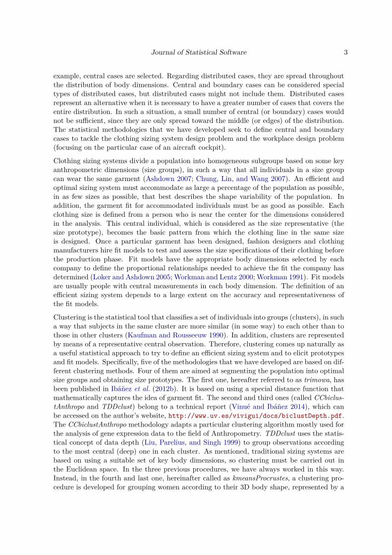
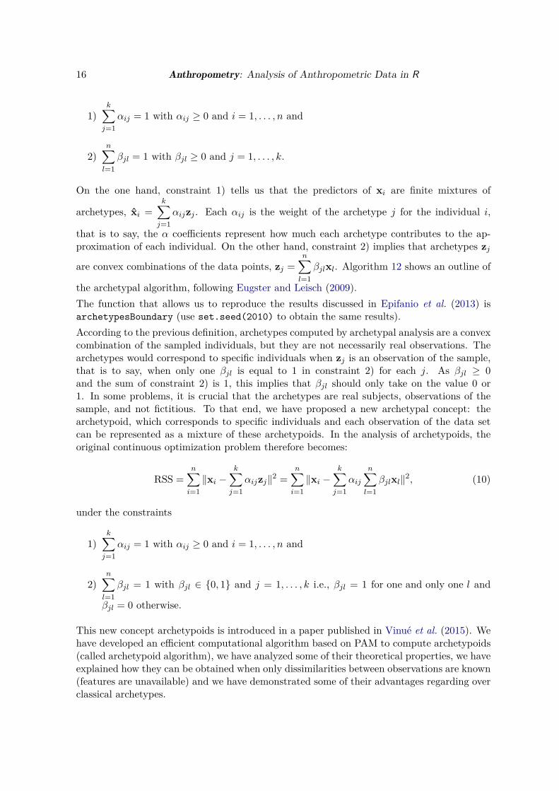
Figure 3 shows the scatter plots of bust circumference against neck to ground with the threeprototypes obtained for each bust class without (left) and with (right) the prototypes definedby the European standard. The prototypes color and the plot title must be provided. Unlikethe European standard prototypes, which are strictly defined for any database, our prototypesare better adapted to the particular body measurements of the sample of individuals belongingto each size.
Journal of Statistical Software 19
*
*
***
*
*
*
*
*
*
*
**
*
***
*
*
*
** *
*
**
*
*
*
*
***
*
*
*
*
*
*
**
*
*
*
*
*
*
*
*
*
**
*
*
*
**
*
*
*
*
*
*
*
**
*
*
*
*
*
**
*
*
**
*
*
*
*
*
*
*
*
*
*
*
*
*
* **
*
**
**
*
*
*
*
*
*
**
*
*
*
*
*
*
*
*
*
*
*
**
*
*
*
*
*
*
*
*
*
*
*
*
*
*
*
*
*
*
*
*
**
*
*
*
*
**
*
**
*
*
*
*
*
*
*
**
**
**
*
*
*
*
*
** *
**
*
*
*
**
**
**
*
*
*
*
*
*
*
*
*
*
*
*
*
*
*
*
*
*
*
*
*
*
*
*
*
*
*
*
*
*
*
*
*
*
*
*
**
*
*
**
**
*
*
*
**
**
*
*
*
*
*
*
*
*
*
*
*
*
*
*
*
*
*
*
*
*
**
*
*
*
*
**
**
**
*
*
*
*
**
*
*
*
*
*
*
*
*
*
*
*
*
**
**
*
*
*
*
*
*
*
*
*
*
*
***
*
*
*
*
*
*
*
*
*
**
*
**
*
*
**
*
*
*
*
*
*
**
*
*
**
**
*
**
**
**
*
*
*
*
*
*
****
*
*
*
*
*
**
**
*
*
*
*
*
*
*
*
*
*
*
**
*
*
*
*
*
**
*
**
*
*
*
* *
*
**
*
*
*
*
*
*
*
*
*
*
**
*
*
*
*
*
*
**
*
*
*
*** *
*
*
**
*
**
*
**
*
*
*
*
*
*
*
*
*
*
*
*
*
*
*
*
**
*
*
*
*
***
*
*
**
*
*
*
*
*
*
*
*
*
**
**
*
* *
*
*
*
*
*
* *
*
*
*
*
**
*
* **
*** *
*
**
*
*
*
*
**
*
**
**
*
*
**
*
*
*
*
*
*
**
*
*
*
*
*
*
*
*
*
**
**
*
*
**
***
**
*
*
*
*
*
*
*
*
*
*
*
**
*
*
*
*
**
*
*
*
*
*
*
*
**
**
*
*
*
*
*
*
*
*
*
* *
*
* *
*
*
*
**
*
*
**
*
*
*
*
*
Prototypes bust vs neck to ground
bust
neck
togr
ound
72 82 92 102 112 122 132
116
126
136
146
156
●
●
●
●
●
●
*
*
***
*
*
*
*
*
*
*
**
*
***
*
*
*
** *
*
**
*
*
*
*
***
*
*
*
*
*
*
**
*
*
*
*
*
*
*
*
*
**
*
*
*
**
*
*
*
*
*
*
*
**
*
*
*
*
*
**
*
*
**
*
*
*
*
*
*
*
*
*
*
*
*
*
* **
*
**
**
*
*
*
*
*
*
**
*
*
*
*
*
*
*
*
*
*
*
**
*
*
*
*
*
*
*
*
*
*
*
*
*
*
*
*
*
*
*
*
**
*
*
*
*
**
*
**
*
*
*
*
*
*
*
**
**
**
*
*
*
*
*
** *
**
*
*
*
**
**
**
*
*
*
*
*
*
*
*
*
*
*
*
*
*
*
*
*
*
*
*
*
*
*
*
*
*
*
*
*
*
*
*
*
*
*
*
**
*
*
**
**
*
*
*
**
**
*
*
*
*
*
*
*
*
*
*
*
*
*
*
*
*
*
*
*
*
**
*
*
*
*
**
**
**
*
*
*
*
**
*
*
*
*
*
*
*
*
*
*
*
*
**
**
*
*
*
*
*
*
*
*
*
*
*
***
*
*
*
*
*
*
*
*
*
**
*
**
*
*
**
*
*
*
*
*
*
**
*
*
**
**
*
**
**
**
*
*
*
*
*
*
****
*
*
*
*
*
**
**
*
*
*
*
*
*
*
*
*
*
*
**
*
*
*
*
*
**
*
**
*
*
*
* *
*
**
*
*
*
*
*
*
*
*
*
*
**
*
*
*
*
*
*
**
*
*
*
*** *
*
*
**
*
**
*
**
*
*
*
*
*
*
*
*
*
*
*
*
*
*
*
*
**
*
*
*
*
***
*
*
**
*
*
*
*
*
*
*
*
*
**
**
*
* *
*
*
*
*
*
* *
*
*
*
*
**
*
* **
*** *
*
**
*
*
*
*
**
*
**
**
*
*
**
*
*
*
*
*
*
**
*
*
*
*
*
*
*
*
*
**
**
*
*
**
***
**
*
*
*
*
*
*
*
*
*
*
*
**
*
*
*
*
**
*
*
*
*
*
*
*
**
**
*
*
*
*
*
*
*
*
*
* *
*
* *
*
*
*
**
*
*
**
*
*
*
*
*
Prototypes bust vs neck to ground
bust
neck
togr
ound
72 82 92 102 112 122 132
116
126
136
146
156
●
●
●
●
●
●
Figure 3: Bust vs. neck to ground, jointly with our medoids (left) and the prototypes definedby the European standard (right).
R> bustVariable <- "bust"R> xlim <- c(72, 132)R> color <- c("black", "red", "green", "blue", "cyan", "brown", "gray",+ "deeppink3", "orange", "springgreen4", "khaki3", "steelblue1")R> variable <- "necktoground"R> ylim <- c(116, 156)R> title <- "Prototypes \n bust vs neck to ground"R> plotPrototypes(dataTrimowa, prototypes, numSizes, bustVariable,+ variable, color, xlim, ylim, title, FALSE)R> plotPrototypes(dataTrimowa, prototypes, numSizes, bustVariable,+ variable, color, xlim, ylim, title, TRUE)
The TDDclust methodology
A basic example of the TDDclust methodology is shown here. Computing data depth is verydemanding. As an illustration, only 25 individuals are selected. In addition, the neck toground, waist and bust variables are selected.
R> dataTDDcl <- sampleSpanishSurvey[1:25, c(2, 3, 5)]R> dataTDDcl_aux <- sampleSpanishSurvey[1:25, c(2, 3, 5)]
In line with trimowa, three size groups are calculated (numClust) and a trimmed proportionis fixed to 0.01 (alpha). The lambda controls the influence the data depth has over theclustering. If lambda is 1, the clustering criterion is equivalent to the average silhouette width.On the contrary, if lambda is 0, it is given by the average relative data depth. Fixing lambdato 0.5 is an intermediate and suggested scenario. A detailed explanation of the consequences

20 Anthropometry: Analysis of Anthropometric Data in R
of different lambda values is given in Jörnsten (2004). Because the depth computation iscostly, we only run the algorithm for five iterations (niter).The other arguments are given by default. A different value for Th may result in the opti-mum clustering not being found (see Jörnsten 2004, p. 75). A different simulated annealingparameter (T0 and simAnn) may change the clustering results obtained.
R> numClust <- 3R> alpha <- 0.01R> lambda <- 0.5R> niter <- 5R> Th <- 0R> T0 <- 0R> simAnn <- 0.9R> set.seed(2014)R> res_TDDcl <- TDDclust(dataTDDcl, numClust, lambda, Th, niter, T0, simAnn,+ alpha, dataTDDcl_aux, verbose = FALSE)
The following code statements allow us to analyze the clustering results, the final value of theoptimal partition and the iteration in which the optimal partition was found, respectively.
R> table(res_TDDcl$NN[1,])
1 2 35 10 9
R> res_TDDcl$Cost
[1] 0.3717631
R> res_TDDcl$klBest
[1] 3
The prototypes are obtained with anthrCases. In addition, the trimmOutl generic functionallows us to obtain the trimmed or outlier observations discarded by each method.
R> prototypes <- anthrCases(res_TDDcl)R> trimmed <- trimmOutl(res_TDDcl)
The hipamAnthropom methodology
The following code statements illustrate how to use the hipamAnthropom methodology. Thesame twelve bust segments as in trimowa are used.
R> dataHipam <- sampleSpanishSurveyR> bust <- dataHipam$bustR> bustSizes <- bustSizesStandard(seq(74, 102, 4), seq(107, 131, 6))
Journal of Statistical Software 21
In this situation, where hipamAnthropom is applied to a sequence of body sizes, this algorithmis used inside the helper function computSizesHipamAnthropom. The HIPAM IMO algorithmis used. It was verified in Vinué et al. (2014a) that HIPAM IMO showed better performance forfinding representative prototypes. The maximum number of clusters that any cluster can bedivided into is fixed to five (maxsplit). In the HIPAM algorithm the number of sub-clustersthat any cluster is potentially divided into is between 2 and maxsplit. A larger maxsplitthan five could result in too many clusters, which is not interesting from the point of view ofthe strategy used by companies to design sizes.The same orness and vector of constants as in trimowa are used.
R> type <- "IMO"R> maxsplit <- 5R> orness <- 0.7R> ah <- c(23, 28, 20, 25, 25)R> set.seed(2013)R> numSizes <- bustSizes$nsizes - 1R> res_hipam <- computSizesHipamAnthropom(dataHipam, bust,+ bustSizes$bustCirc, numSizes, maxsplit, orness, type, ah, FALSE)
The fit models are the clustering medoids and the outliers are the discarded observations.
R> fitmodels <- anthrCases(res_hipam, numSizes)R> outliers <- trimmOutl(res_hipam, numSizes)
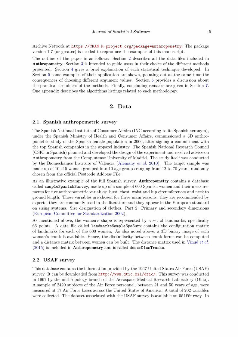
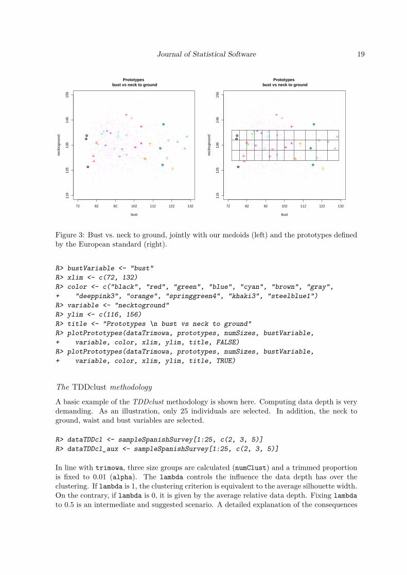
Figure 4 displays the fit models (left) and the outliers (right) corresponding to each bust size.The fit models color and the plot title must be provided. The important point to note hereis the fact that each bust segment has a small sample size. This might explain the fact thatthis algorithm (and also HIPAM MO) does not find large homogeneous clusters and thereforeidentifies a lot of women as outliers in each class for this database. One of the features ofthe HIPAM algorithm is that it is a very sensitive algorithm for identifying outliers. A broaddiscussion, analysis and thoughts on the anthropometric meaning of these outliers is given inVinué et al. (2014a) (including the supplementary material).
R> bustVariable <- "bust"R> xlim <- c(72, 132)R> color <- c("black", "red", "green", "blue", "cyan", "brown", "gray",+ "deeppink3", "orange", "springgreen4", "khaki3", "steelblue1")R> variable <- "hip"R> ylim <- c(83, 153)R> title <- "Fit models HIPAM_IMO \n bust vs hip"R> title_outl <- "Outlier women HIPAM_IMO \n bust vs hip"R> plotPrototypes(dataHipam, fitmodels, numSizes, bustVariable,+ variable, color, xlim, ylim, title, FALSE)R> plotTrimmOutl(dataHipam, outliers, numSizes, bustVariable,+ variable, color, xlim, ylim, title_outl)
The kmeansProcrustes methodologyTo conclude this Section, the use of the kmeansProcrustes methodology is illustrated. For the

22 Anthropometry: Analysis of Anthropometric Data in R
*
*
**
*
* *
* *
*
*
*
*
*
*
*
*
*
*
***
**
*
*
**
**
*
*
****
*
*
*
*
*
*
*
**
**
*
*
*
***
*
*
*
*****
*
**
*
****
*
**
** *
*
***
*
*
*
*
**
*
*
*
*
**
***
*
*
*
*
*
**
*
**
*
**
*
*
*
*
*
*
*
*
* ** ***
*
* *
*
**
*
* *
*
**** *
**
*
**
*
**
*
*
*
**
*
*
*
**
*
*
*
*
**
*
*
**
*
*
*
*
*
**
***
*
**
*
*
* *
* *
*
*
*
*
*
*
*
**
**
***
*
*
*
**
*
**
*
****
**
*
*
*
*
* *
*
***
*
*
*
*
*
*
*
*
*
*
*
*
*
*
**
*
*
*
**
*
*
*
*
*
*
**
*
*
*
**
***
**
***
**
* ***
*
*
*
*
*
*
*
*
*
**
*
*
*
*
*
*
*
*
*
**
***
**
*
**
*
*
****
*
*
*
**
*
**
*
*
**
*
**
*
**
* **
**
* *
*
*
*
*
*
**
*
*
* *
**
**
*
*
*
**
**
**
*
*
*
*
**
***
*
**
*
*
*
***
*
*
*
*
**
*
*
*
*
*
*
*
*
**
****
**
**
*
**
*
*
*
*
*
*
*
**
*
*
* *
*
*
*
* *
**
**
*
*
*
*
**
*
***
*
*
*
**
*
*
* *
*
*
**
**
**
**
**
**
*
*
*
*
*
*
*
*
*
*
*
*
*
*
*
**
**
*
*
*
*
*
*
*
*
**
*
*
*
*
*
*
**
*
**
*
*
*
**
*
*
*
*
*
*
*
*
***
* ** *
*
*
*
**
*
*
*
*
*
*
****
**
*
*
*
*
*
** *
*
**
*
*
*
*
*
*
*
*
*** **
*
*
*
*
**
**
*
*
**
*
*
** *
*
**
*
*
*
**
**
*
*
* *
**
*
*
*
* *
*
*
*
*
*
*
Fit models HIPAM_IMO bust vs hip
bust
hip
72 82 92 102 112 122 132
8393
103
113
123
133
143
153
●
*
*
**
*
* *
* *
*
*
*
*
*
*
*
*
*
*
***
**
*
*
**
**
*
*
****
*
*
*
*
*
*
*
**
**
*
*
*
***
*
*
*
*****
*
**
*
****
*
**
** *
*
***
*
*
*
*
**
*
*
*
*
**
***
*
*
*
*
*
**
*
**
*
**
*
*
*
*
*
*
*
*
* ** ***
*
* *
*
**
*
* *
*
**** *
**
*
**
*
**
*
*
*
**
*
*
*
**
*
*
*
*
**
*
*
**
*
*
*
*
*
**
***
*
**
*
*
* *
* *
*
*
*
*
*
*
*
**
**
***
*
*
*
**
*
**
*
****
**
*
*
*
*
* *
*
***
*
*
*
*
*
*
*
*
*
*
*
*
*
*
**
*
*
*
**
*
*
*
*
*
*
**
*
*
*
**
***
**
***
**
* ***
*
*
*
*
*
*
*
*
*
**
*
*
*
*
*
*
*
*
*
**
***
**
*
**
*
*
****
*
*
*
**
*
**
*
*
**
*
**
*
**
* **
**
* *
*
*
*
*
*
**
*
*
* *
**
**
*
*
*
**
**
**
*
*
*
*
**
***
*
**
*
*
*
***
*
*
*
*
**
*
*
*
*
*
*
*
*
**
****
**
**
*
**
*
*
*
*
*
*
*
**
*
*
* *
*
*
*
* *
**
**
*
*
*
*
**
*
***
*
*
*
**
*
*
* *
*
*
**
**
**
**
**
**
*
*
*
*
*
*
*
*
*
*
*
*
*
*
*
**
**
*
*
*
*
*
*
*
*
**
*
*
*
*
*
*
**
*
**
*
*
*
**
*
*
*
*
*
*
*
*
***
* ** *
*
*
*
**
*
*
*
*
*
*
****
**
*
*
*
*
*
** *
*
**
*
*
*
*
*
*
*
*
*** **
*
*
*
*
**
**
*
*
**
*
*
** *
*
**
*
*
*
**
**
*
*
* *
**
*
*
*
* *
*
*
*
*
*
*
Outlier women HIPAM_IMO bust vs hip
bust
hip
72 82 92 102 112 122 132
8393
103
113
123
133
143
153
●
●
●
●
●
●
●
●
●●●
●
●
●
●
●
●
●
●
●
●
●
●
●
●
●●
●
●●
●●
●
Figure 4: Bust vs. hip with the medoids (left) and with the outliers (right) obtained usingHIPAM IMO.
sake of simplicity of the computation involved only a small sample (the first 50 individuals)is selected. When there are missing values (NA’s, not available numbers), they are removed.
R> landmarksNoNa <- na.exclude(landmarksSampleSpaSurv)R> numLandmarks <- (dim(landmarksNoNa)[2]) / 3R> landmarksNoNa_First50 <- landmarksNoNa[1:50, ]R> numIndiv <- dim(landmarksNoNa_First50)[1]
We have to define an array with the 3D landmarks of the sample objects.
R> array3D <- array3Dlandm(numLandmarks, numIndiv, landmarksNoNa_First50)
Again, three size groups are calculated (numClust) and a trimmed proportion is fixed to0.01 (alpha). The trimmedLloydShapes algorithm is used with only five iterations and fivesteps per initialization in the interests of a fast execution. A larger number of repetitionsis suggested to obtain more optimal results. The default relative stopping criteria is 0.0001.Using this small value ensures that the algorithm stops when the decrease in the objectivefunction is hardly visible. A larger stopping value could prematurely stop the algorithm (butthe decrease in the objective function should have been taken into account).
R> numClust <- 3R> alpha <- 0.01R> algSteps <- 5R> niter <- 5R> stopCr <- 0.0001R> set.seed(2013)R> res_kmProc <- trimmedLloydShapes(array3D, numIndiv, alpha, numClust,+ algSteps, niter, stopCr, verbose = FALSE)
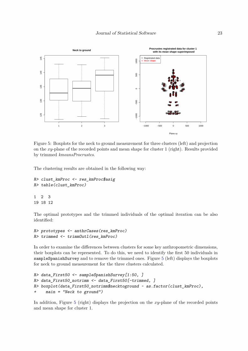
Journal of Statistical Software 23
1 2 3
125
130
135
140
145
Neck to ground
−1000 −500 0 500 1000
−10
00−
500
050
010
00
Registrated dataMean shape
Procrustes registrated data for cluster 1 with its mean shape superimposed
Plane xy
Figure 5: Boxplots for the neck to ground measurement for three clusters (left) and projectionon the xy-plane of the recorded points and mean shape for cluster 1 (right). Results providedby trimmed kmeansProcrustes.
The clustering results are obtained in the following way:
R> clust_kmProc <- res_kmProc$asigR> table(clust_kmProc)
1 2 319 18 12
The optimal prototypes and the trimmed individuals of the optimal iteration can be alsoidentified:
R> prototypes <- anthrCases(res_kmProc)R> trimmed <- trimmOutl(res_kmProc)
In order to examine the differences between clusters for some key anthropometric dimensions,their boxplots can be represented. To do this, we need to identify the first 50 individuals insampleSpanishSurvey and to remove the trimmed ones. Figure 5 (left) displays the boxplotsfor neck to ground measurement for the three clusters calculated.
R> data_First50 <- sampleSpanishSurvey[1:50, ]R> data_First50_notrimm <- data_First50[-trimmed, ]R> boxplot(data_First50_notrimm$necktoground ~ as.factor(clust_kmProc),+ main = "Neck to ground")
In addition, Figure 5 (right) displays the projection on the xy-plane of the recorded pointsand mean shape for cluster 1.

24 Anthropometry: Analysis of Anthropometric Data in R
R> projShapes(1, array3D, clust_kmProc, prototypes)R> legend("topleft", c("Registrated data", "Mean shape"),+ pch = 1, col = 1:2, text.col = 1:2)R> title("Procrustes registrated data for cluster 1 \n+ with its mean shape superimposed", sub = "Plane xy")
5.2. Archetypal analysis
We focus on the cockpit design problem. The accommodation of boundaries (our archety-poids) ensures the accommodation of interior points in the cockpit. We use the USAFSurveydatabase. Again, as an illustrative example only the first 50 individuals are chosen. From thetotal variables, the six so-called cockpit dimensions are selected. They are thumb tip reach,buttock-knee length, popliteal height sitting, sitting height, eye height sitting and shoulderheight sitting. We convert the variables from mm into inches in order to compare our resultswith those discussed in Zehner et al. (1993) (see Epifanio et al. 2013, for more details). Theprocedure followed for each problem is as follows:Before computing archetypes and archetypoids, the data must be preprocessed. Firstly, de-pending on the problem, the user must decide whether or not to standardize the data. Sec-ondly, it must be decided whether to use the Mahalanobis distance or a depth procedure toestablish the percentage of the population to accommodate (see Epifanio et al. 2013, Section2.2.2 for more details). Both actions are done with the following preprocessing function. Inthis case, the variables are standardized, as they measure different dimensions. This is indi-cated with the first TRUE argument in preprocessing. On the other hand, when designing aworkspace, it has typically been a requirement that 95 percent of the relevant population areaccommodated (value 0.95 in the third argument). Finally, the second TRUE (and fourth andfinal parameter) indicates that the Mahalanobis distance is used to remove the most extreme5% data.
R> USAFSurvey_First50 <- USAFSurvey[1:50, ]R> variabl_sel <- c(48, 40, 39, 33, 34, 36)R> USAFSurvey_First50_inch <- USAFSurvey_First50[,variabl_sel] / (10 * 2.54)R> USAFSurvey_preproc <- preprocessing(data = USAFSurvey_First50_inch,+ stand = TRUE, percAccomm = 0.95, mahal= TRUE)
Next, archetypes must be calculated. In the archetypes R package (Eugster, Leisch, andSeth 2014; Eugster and Leisch 2009) this is done with the stepArchetypes function, whichexecutes the archetype algorithm repeatedly. However, this function standardizes the databy default and this option is not always desired. To overcome this, a new R function calledstepArchetypesRawData has been written, which results from modifying and adapting theoriginal stepArchetypes to apply the archetype algorithm to raw data. In this way, thearchetype algorithm is run repeatedly from 1 to numArch archetypes. The user can decidehow many archetypes are to be considered. We chose numArch equal to 10 because a largernumber of boundary cases may overwhelm the designer and therefore be counterproductive.The argument numRep specifies the number of repetitions of the algorithm. Choosing twentyrepetitions ensures that the best possible archetypes are obtained. Note that in some stepsof the algorithm singular linear equation systems may occur leading to warnings for somenumArch values (as in Eugster and Leisch 2009, p. 9).
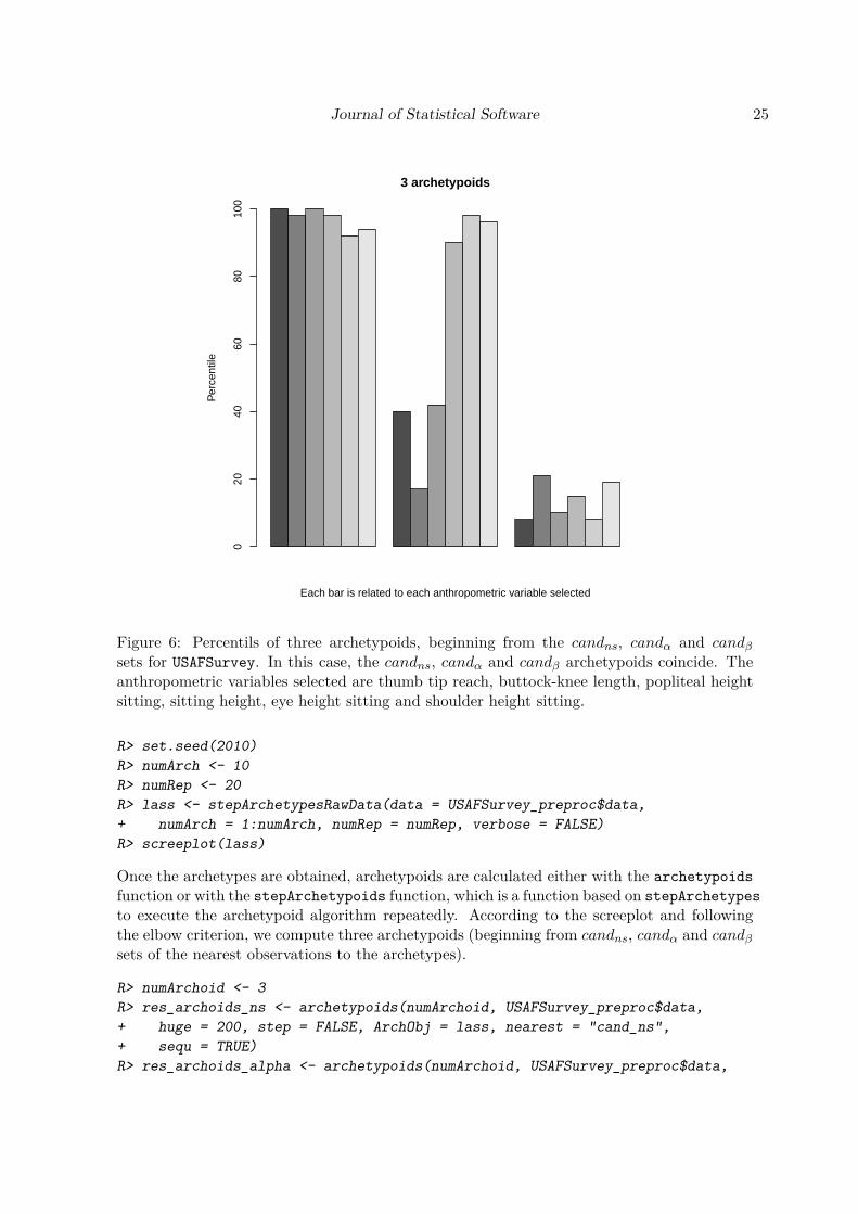
Journal of Statistical Software 25
3 archetypoids
Each bar is related to each anthropometric variable selected
Per
cent
ile
020
4060
8010
0
Figure 6: Percentils of three archetypoids, beginning from the candns, candα and candβsets for USAFSurvey. In this case, the candns, candα and candβ archetypoids coincide. Theanthropometric variables selected are thumb tip reach, buttock-knee length, popliteal heightsitting, sitting height, eye height sitting and shoulder height sitting.
R> set.seed(2010)R> numArch <- 10R> numRep <- 20R> lass <- stepArchetypesRawData(data = USAFSurvey_preproc$data,+ numArch = 1:numArch, numRep = numRep, verbose = FALSE)R> screeplot(lass)
Once the archetypes are obtained, archetypoids are calculated either with the archetypoidsfunction or with the stepArchetypoids function, which is a function based on stepArchetypesto execute the archetypoid algorithm repeatedly. According to the screeplot and followingthe elbow criterion, we compute three archetypoids (beginning from candns, candα and candβsets of the nearest observations to the archetypes).
R> numArchoid <- 3R> res_archoids_ns <- archetypoids(numArchoid, USAFSurvey_preproc$data,+ huge = 200, step = FALSE, ArchObj = lass, nearest = "cand_ns",+ sequ = TRUE)R> res_archoids_alpha <- archetypoids(numArchoid, USAFSurvey_preproc$data,

26 Anthropometry: Analysis of Anthropometric Data in R
+ huge = 200, step = FALSE, ArchObj = lass, nearest = "cand_alpha",+ sequ = TRUE)R> res_archoids_beta <- archetypoids(numArchoid, USAFSurvey_preproc$data,+ huge = 200, step = FALSE, ArchObj = lass, nearest = "cand_beta",+ sequ = TRUE)R> boundaries_ns <- anthrCases(res_archoids_ns)R> boundaries_alpha <- anthrCases(res_archoids_alpha)R> boundaries_beta <- anthrCases(res_archoids_beta)
In this case, the candns, candα and candβ archetypoids match (although the candns, candαand candβ archetypes do not), so it is enough to represent a single percentile plot. To that end,the percentilsArchetypoid computes the percentiles of the archetypoids for every columnof the data frame.
R> df <- USAFSurvey_preproc$dataR> matPer <- t(sapply(1:dim(df)[2], percentilsArchetypoid,+ boundaries_ns, df, 0))
Figure 6 shows the percentils of three archetypoids.
R> barplot(matPer, beside = TRUE, main = paste(numArchoid,+ " archetypoids", sep = ""), ylim = c(0, 100), ylab = "Percentile",+ xlab = "Each bar is related to each anthropometric variable selected")
6. DiscussionProcedures related to clustering, data depth and shape analysis (trimowa, CCbiclustAnthropo,hipamAnthropom, TDDclust and kmeansProcrustes) are aimed at defining optimal clothingsize groups and both 1D and 3D central cases, which are actually representative statisticalmodels or prototypes (and fit models in the case of hipamAnthropom) of the human bodyof the target population. The five aforementioned methodologies followed the same scheme.Firstly, the selected data matrix was segmented using a primary control dimension (bustor waist) and then a further segmentation was carried out using other secondary controlanthropometric variables. The number of size groups generally obtained with these methodswas three, because this number is quite well aligned to clothing industry practice for the massproduction of clothing, where the objective is to optimize sizes by addressing only the mostprofitable. This procedure can be translated into practice as shown in Figure 7.For a given bust size, for example, 86–90 cm, the three T-shirts in Figure 7 were designed fromthe three prototypes obtained by any of the aforementioned methodologies. It can be seenthat all three have the same bust size (primary dimension), but different measurements forother secondary dimensions (in this example, waist and neck-to-hip are selected for illustrativepurposes). In a commercial situation, a woman in a store would directly select the T-shirtswith her bust size and, out of all of them, she would finally choose the one with her samemeasurements for the other secondary variables. As a result, the customer would have quicklyand easily found a T-shirt that fits perfectly. It is believed that the statistical methodologiespresented here can speed up the purchasing process, making it more satisfactory. Figure 7 also

Journal of Statistical Software 27
Figure 7: Practical implementation of the methodologies presented. These are three T-shirtsdesigned from the prototypes obtained. The three T-shirts have the same bust size (primarydimension), but different measurements for other secondary dimensions. This method ofdesigning and labelling may speed up the purchasing process, making it more satisfactory.
shows a proposal for garment labelling. Clothing fit depends a lot on better garment labelling.Apparel companies should offer consumers truthful information that is not confusing on thegarment sizes that they wish to offer for sale, so that people can easily recognize their size. Inaddition, the prototypes and fit models obtained can also be used to make more realistic storemannequins, thus helping to offer an image of healthy beauty in society, which is another veryuseful and practical application.On the other hand, the two approaches based on archetypal and archetypoid analysis makeit possible to identify boundary cases, that is to say, the individuals who present extremebody measurements. The basic idea is that accommodating boundary cases will accommo-date the people who fall within the boundaries (less extreme population). This strategy isvaluable in all human-computer interaction problems, for example, the design and packagingof plane cockpits or truck cabins. When designing workstations or evaluating manual work,it is common to use only a few human figure models (extreme cases, which would be ourarchetypoids) as virtual test individuals. These models are capable of representing peoplewith a wide range of body sizes and shapes. Archetypal and archetypoid analysis can be veryuseful in improving industry practice when using human model tools to design products andwork environments.
7. ConclusionsNew three-dimensional whole-body scanners have drastically reduced the cost and durationof the measurement process. These types of systems, in which the human body is digitallyscanned and the resulting data converted into exact measurements, make it possible to obtainaccurate, reproducible and up-to-date anthropometric data. These databases constitute veryvaluable information to effectively design better-fitting clothing and workstations, to under-stand the body shape of the population and to reduce the design process cycle. Therefore,rigorous statistical methodologies and software applications must be developed to make themost of them.This paper introduces a new R package called Anthropometry that brings together differentstatistical methodologies concerning clustering, the statistical concept of data depth, statisti-

28 Anthropometry: Analysis of Anthropometric Data in R
cal shape analysis and archetypal analysis, which have been especially developed to deal withanthropometric data. The data used have been obtained from a 3D anthropometric surveyof the Spanish female population and from the USAF survey. Procedures related to cluster-ing, data depth and shape analysis are aimed at defining optimal clothing size groups andboth central prototypes and fit models. The two approaches based on archetypal analysis areuseful for determining boundary human models which could be useful for improving industrypractice in workspace design.The Anthropometry R package is a positive contribution to help tackle some statistical prob-lems related to Ergonomics and Anthropometry. It provides a useful software tool for engi-neers and researchers in these fields so that they can analyze their anthropometric data in acomprehensive way.
AcknowledgmentsThe author gratefully acknowledges the many helpful suggestions of I. Epifanio and G. Ayala.The author would also like to thank the Biomechanics Institute of Valencia for providingus with the Spanish anthropometric data set and the Spanish Ministry of Health and Con-sumer Affairs for having commissioned and coordinated the “Anthropometric Study of theFemale Population in Spain”. This paper has been partially supported by the following grants:TIN2009-14392-C02-01, TIN2009-14392-C02-02. The author would also like to thank the ed-itors and referee for their very constructive suggestions, which led to a great improvement ofboth this paper and the Anthropometry package.
References
Alemany S, González JC, Nácher B, Soriano C, Arnáiz C, Heras H (2010). “AnthropometricSurvey of the Spanish Female Population Aimed at the Apparel Industry.” In Proceedingsof the 2010 International Conference on 3D Body Scanning Technologies. Lugano, Switzer-land.
Arenas C, Cuadras M (2002). “Recent Statistical Methods Based on Distances.” Contributionsto Science, 2(2), 183–191. URL http://revistes.iec.cat/index.php/CtS/article/view/297/296.
Ashdown SP (2007). Sizing in Clothing: Developing Effective Sizing Systems for Ready-To-Wear Clothing. Woodhead Publishing in Textiles.
Bagherzadeh R, Latifi M, Faramarzi AR (2010). “Employing a Three-Stage Data MiningProcedure to Develop Sizing System.” World Applied Sciences Journal, 8(8), 923–929.URL http://www.idosi.org/wasj/wasj8(8)10/2.pdf.
Bertilsson E, Högberg D, Hanson L (2012). “Using Experimental Design to Define BoundaryManikins.” Work: A Journal of Prevention, Assessment and Rehabilitation, 41(Supplement1), 4598–4605. doi:10.3233/WOR-2012-0075-4598.

Journal of Statistical Software 29
Bittner AC, Glenn FA, Harris RM, Iavecchia HP, Wherry RJ (1987). “CADRE: A Familyof Manikins for Workstation Design.” In Asfour, S.S. (Ed.) Trends in Ergonomics/HumanFactors IV. North Holland, pp. 733–740.
Blanchonette P (2010). “Jack Human Modelling Tool: A Review.” Technical Report DSTO-TR-2364, Defence Science and Technology Organisation (Australia). Air Operations Divi-sion.
Cheng Y, Church GM (2000). “Biclustering of Expression Data.” Proceedings of the EighthInternational Conference on Intelligent Systems for Molecular Biology, 8, 93–103.
Chung MJ, Lin HF, Wang MJJ (2007). “The Development of Sizing Systems for TaiwaneseElementary- And High-School Students.” International Journal of Industrial Ergonomics,37, 707–716. doi:10.1016/j.ergon.2007.05.004.
Cutler A, Breiman L (1994). “Archetypal Analysis.” Technometrics, 36(4), 338–347. doi:10.1080/00401706.1994.10485840.
D’Apuzzo N (2009). Recent Advances in 3D Full Body Scanning with Applications to Fashionand Apparel. Gruen, A., Kahmen, H. (eds.). Optical 3-D Measurement Techniques IX.
Ding Y, Dang X, Peng H, Wilkins D (2007). “Robust Clustering in High Dimensional DataUsing Statistical Depths.” BMC Bioinformatics, 8(Suppl 7:S8), 1–16.
Dryden IE, Mardia KV (1998). Statistical Shape Analysis. John Wiley & Sons. doi:10.1002/9781119072492.
Dutta D, Ghosh AK (2012). “On Robust Classification Using Projection Depth.” Annals of theInstitute of Statistical Mathematics, 64(3), 657–676. doi:10.1007/s10463-011-0324-y.
Epifanio I, Vinué G, Alemany S (2013). “Archetypal Analysis: Contributions for Estimat-ing Boundary Cases in Multivariate Accommodation Problem.” Computers & IndustrialEngineering, 64, 757–765.
Eugster MJ (2012). “Performance Profiles Based on Archetypal Athletes.” InternationalJournal of Performance Analysis in Sport, 12(1), 166–187. doi:10.1080/24748668.2012.11868592.
Eugster MJ, Leisch F (2009). “From Spider-Man to Hero – Archetypal Analysis in R.” Journalof Statistical Software, 30(8), 1–23. doi:10.18637/jss.v030.i08.
Eugster MJ, Leisch F, Seth S (2014). archetypes: Archetypal Analysis. R package version2.2-0, URL https://CRAN.R-project.org/package=archetypes.
European Committee for Standardization (2002). “Size Designation of Clothes. Part 2: Pri-mary and Secondary Dimensions.”
European Committee for Standardization (2005). “Size Designation of Clothes. Part 3: Mea-surements and Intervals.”
Friess M (2005). “Multivariate Accommodation Models Using Traditional and 3D Anthro-pometry.” Technical report, SAE. doi:10.4271/2005-01-2735.

30 Anthropometry: Analysis of Anthropometric Data in R
Friess M, Bradtmiller B (2003). “3D Head Models for Protective Helmet Development.”Technical report, SAE. doi:10.4271/2003-01-2176.
García-Escudero LA, Gordaliza A, Matrán C (2003). “Trimming Tools in Exploratory DataAnalysis.” Journal of Computational and Graphical Statistics, 12(2), 434–449.
García-Escudero LA, Gordaliza A, Matrán C, Mayo-Iscar A (2008). “A General TrimmingApproach to Robust Cluster Analysis.” The Annals of Statistics, 36, 1324–1345.
Gupta D, Gangadhar BR (2004). “A Statistical Model for Developing Body Size Chartsfor Garments.” International Journal of Clothing Science and Technology, 16(5), 458–469.doi:10.1108/09556220410555641.
HFES 300 Committee (2004). Guidelines for Using Anthropometric Data in Product Design.Human Factors and Ergonomics Society.
Hsu CH (2009a). “Data Mining to Improve Industrial Standards and Enhance Production andMarketing: An Empirical Study in Apparel Industry.” Expert Systems with Applications,36, 4185–4191.
Hsu CH (2009b). “Developing Accurate Industrial Standards to Facilitate Production inApparel Manufacturing Based on Anthropometric Data.” Human Factors and Ergonomicsin Manufacturing, 19(3), 199–211.
Hudson JA, Zehner GF, Meindl RD (1998). “The USAF Multivariate AccommodationMethod.” Proceedings of the Human Factors and Ergonomics Society Annual Meeting,42(10), 722–726.
Ibáñez MV, Simó A, Domingo J, Durá E, Ayala G, Alemany S, Vinué G, Solves C (2012a).“A Statistical Approach to Build 3D Prototypes from a 3D Anthropometric Survey ofthe Spanish Female Population.” In Proceedings of the 1st International Conference onPattern Recognition Applications and Methods, volume 1, pp. 370–374. Vilamoura, Algarve,Portugal.
Ibáñez MV, Vinué G, Alemany S, Simó A, Epifanio I, Domingo J, Ayala G (2012b). “ApparelSizing Using Trimmed PAM and OWA Operators.” Expert Systems with Applications, 39,10512–10520. doi:10.1016/j.eswa.2012.02.127.
Irigoien I, Arenas C (2008). “INCA: New Statistic for Estimating the Number of Clustersand Identifying Atypical Units.” Statistics in Medicine, 27, 2948–2973.
Irigoien I, Sierra B, Arenas C (2012). “ICGE: An R Package for Detecting Relevant Clustersand Atypical Units in Gene Expression.” Bioinformatics, 13(30), 1–11.
Istook CL, Hwang SJ (2001). “3D Body Scanning Systems with Application to the ApparelIndustry.” Journal of Fashion Marketing and Management, 5, 120–132. doi:10.1108/eum0000000007283.
Jörnsten R (2004). “Clustering and Classification Based on the L1 Data Depth.” Journal ofMultivariate Analysis, 90, 67–89. doi:10.1016/j.jmva.2004.02.013.

Journal of Statistical Software 31
Jörnsten R, Vardi Y, Zhang CH (2002). “A Robust Clustering Method and Visualization ToolBased on Data Depth.” In Statistical Data Analysis Based on the L1-Norm and RelatedMethods (Neuchâtel, 2002), Statistics for Industry and Technology, pp. 353–366.
Kaiser S, Leisch F (2008). “A Toolbox for Bicluster Analysis in R.” Technical report, De-partment of Statistics (University of Munich). URL https://core.ac.uk/download/pdf/12164184.pdf.
Kaiser S, Santamaria R, Khamiakova T, Sill M, Theron R, Quintales L, Leisch F (2015).biclust: BiCluster Algorithms. R package version 1.2.0, URL https://CRAN.R-project.org/package=biclust.
Kaufman L, Rousseeuw PJ (1990). Finding Groups in Data: An Introduction to ClusterAnalysis. John Wiley & Sons. doi:10.1002/9780470316801.
Lange T, Mosler K, Mozharovskyi P (2012). “Fast Nonparametric Classification Based onData Depth.” Statistical Papers, 5, 1–22. doi:10.1007/s00362-012-0488-4.
Lerch T, MacGillivray M, Domina T (2007). “3D Laser Scanning: A Model of Multidisci-plinary Research.” Journal of Textile and Apparel, Technology and Management, 5, 1–22.
Liu RY, Parelius JM, Singh K (1999). “Multivariate Analysis by Data Depth: DescriptiveStatistics, Graphics and Inference.” The Annals of Statistics, 27(3), 783–858. doi:10.1214/aos/1018031260.
Loker S, Ashdown S (2005). “Improved Apparel Sizing: Fit and Anthropometric 3D ScanData.” Technical report, National Textile Center Annual Report.
Loker S, Ashdown S, Schoenfelder K (2005). “Size-Specific Analysis of Body Scan Data toImprove Apparel Fit.” Journal of Textile and Apparel, Technology and Management, 4(3),1–15.
Lu JM, Wang MJJ (2008). “Automated Anthropometric Data Collection Using 3D WholeBody Scanners.” Expert Systems with Applications, 35, 407–414. doi:10.1016/j.eswa.2007.07.008.
Luximon A, Zhang Y, Luximon Y, Xiao M (2012). “Sizing and Grading for Wearable Prod-ucts.” Computer-Aided Design, 44, 77–84.
Madeira SC, Oliveira AL (2004). “Biclustering Algorithms for Biological Data Analysis:A Survey.” IEEE Transactions on Computational Biology and Bioinformatics, 1, 24–45.doi:10.1109/tcbb.2004.2.
McCulloch CE, Paal B, Ashdown SP (1998). “An Optimization Approach to Apparel Sizing.”Journal of the Operational Research Society, 49, 492–499. doi:10.1057/palgrave.jors.2600533.
Moroney WF, Smith MJ (1972). “Empirical Reduction in Potential User Population As theResult of Imposed Multivariate Anthropometric Limits.” Technical report, Naval AerospaceMedical Research Laboratory.

32 Anthropometry: Analysis of Anthropometric Data in R
Pan JZ, Jörnsten R, Hart RP (2004). “Screening Anti-Inflammatory Compounds in InjuredSpinal Cord with Microarrays: A Comparison of Bioinformatics Analysis Approaches.”Physiological Genomics, 17, 201–214.
Parkinson MB, Reed MP, Kokkolaras M, Papalambros PY (2006). “Optimizing Truck CabLayout for Driver Accommodation.” Journal of Mechanical Design, 129(11), 1110–1117.
Pheasant S (2003). Bodyspace: Anthropometry, Ergonomics and the Design of Work. Taylor& Francis, Ltd.
R Core Team (2017). R: A Language and Environment for Statistical Computing. R Founda-tion for Statistical Computing, Vienna, Austria. URL https://www.R-project.org/.
Robinette KM, McConville JT (1981). “An Alternative to Percentile Models.” Technicalreport, SAE. doi:10.4271/810217.
Robinson JC, Robinette KM, Zehner GF (1992). “User’s Guide to the AnthropometricDatabase at the Computerized Anthropometric Research and Design (CARD) Labora-tory.” Technical report, Systems Research Laboratories. URL http://oai.dtic.mil/oai/oai?verb=getRecord&metadataPrefix=html&identifier=ADA273002.
Romo J, López A (2010). “Simplicial Similarity and Its Application to Hierarchical Clus-tering.” Technical report, Universidad Carlos III de Madrid. Departamento de Estadís-tica. Working papers. Statistics and Econometrics. URL http://EconPapers.repec.org/RePEc:cte:wsrepe:ws102915.
Seiler C, Wohlrabe K (2013). “Archetypal Scientists.” Journal of Informetrics, 7, 345–356.doi:10.1016/j.joi.2012.11.013.
Shu C, Wuhrer S, Xi P (2011). “Geometric and Statistical Methods for Processing 3D An-thropometric Data.” In International Symposium on Digital Human Modeling.
Simmons KP, Istook CL (2003). “Body Measurement Techniques: Comparing 3D Body-Scanning and Anthropometric Methods for Apparel Applications.” Journal of FashionMarketing and Management, 7(3), 306–332. doi:10.1108/13612020310484852.
Song HK, Ashdown SP (2010). “An Exploratory Study of the Validity of Visual Fit As-sessment From Three-Dimensional Scans.” Clothing and Textiles Research Journal, 28(4),263–278.
Tryfos P (1986). “An Integer Programming Approach to the Apparel Sizing Problem.” TheJournal of the Operational Research Society, 37(10), 1001–1006.
Vardi Y, Zhang CH (2000). “The Multivariate L1-Median and Associated Data Depth.”Proceedings of the National Academy of Sciences, 97, 1423–1426. doi:10.1073/pnas.97.4.1423.
Vinué G (2012). Métodos Biclustering Aplicados a Datos Antropométricos: Exploración De SuPosible Aplicación En El Diseño De Indumentaria. Master’s thesis, School of Mathematics,University of Valencia (Spain). In Spanish.

Journal of Statistical Software 33
Vinué G (2014). Development of Statistical Methodologies Applied to Anthropometric DataOriented Towards the Ergonomic Design of Products. Ph.D. thesis, Faculty of Mathematics.University of Valencia, Spain, http://hdl.handle.net/10550/35907.
Vinué G, Epifanio I, Alemany S (2015). “Archetypoids: A New Approach to Define Repre-sentative Archetypal Data.” Computational Statistics & Data Analysis, 87, 102–115.
Vinué G, Ibáñez MV (2014). “Data Depth and Biclustering Applied to Anthropometric Data:Exploring Their Utility in Apparel Design.” Technical report, URL http://www.uv.es/vivigui/docs/biclustDepth.pdf.
Vinué G, León T, Alemany S, Ayala G (2014a). “Looking for Representative Fit Models forApparel Sizing.” Decision Support Systems, 57, 22–33.
Vinué G, Simó A, Alemany S (2014b). “The k-Means Algorithm for 3D Shapes with anApplication to Apparel Design.” Advances in Data Analysis and Classification, pp. 1–30.doi:10.1007/s11634-014-0187-1.
Wang MJJ, Wu WY, Lin KC, Yang SN, Lu JM (2007). “Automated Anthropometric DataCollection from Three-Dimensional Digital Human Models.” The International Journal ofAdvanced Manufacturing Technology, 32, 109–115. doi:10.1007/s00170-005-0307-3.
Weiszfeld E, Plastria F (2009). “On the Point for Which the Sum of the Distances to nGiven Points Is Minimum.” Annals of Operations Research, 167, 7–41. doi:10.1007/s10479-008-0352-z.
Wit E, McClure J (2004). Statistics for Microarrays: Design, Analysis and Inference. JohnWiley & Sons.
Workman J (1991). “Body Measurement Specifications for Fit Models As a Factor in ClothingSize Variation.” Clothing and Textiles Research Journal, 10(1), 31–36.
Workman JE, Lentz ES (2000). “Measurement Specifications for Manufacturers’ PrototypeBodies.” Clothing and Textiles Research Journal, 18(4), 251–259.
Yager RR (1988). “On Ordered Weighted Averaging Aggregation Operators in Multi-CriteriaDecision Making.” IEEE Transactions on Systems, Man and Cybernetics, 18, 183–190.doi:10.1109/21.87068.
Zehner GF, Meindl RS, Hudson JA (1993). “A Multivariate Anthropometric Method for CrewStation Design: Abridged.” Technical report, Human Engineering Division, ArmstrongLaboratory, Wright-Patterson Air Force Base, Ohio. URL http://www.dtic.mil/dtic/tr/fulltext/u2/a274588.pdf.
Zheng R, Yu W, Fan J (2007). “Development of a New Chinese Bra Sizing System Based onBreast Anthropometric Measurements.” International Journal of Industrial Ergonomics,37, 697–705.
Zuo Y (2006). “Multidimensional Trimming Based on Projection Depth.” The Annals ofStatistics, 34(5), 2211–2251. doi:10.1214/009053606000000713.
Zuo Y, Serfling R (2000). “General Notions of Statistical Depth Function.” The Annals ofStatistics, 28(2), 461–482. doi:10.1214/aos/1016218226.

34 Anthropometry: Analysis of Anthropometric Data in R
A. Algorithm listings
Algorithm 3 trimowa algorithm.1. Set k, number of groups; algSteps, number of repetitions to find optimal medoids; and niter,number of repetitions of the whole algorithm.2. Select k starting points that will serve as seed medoids (e.g., draw at random k subjects fromthe whole data set).for r = 1→ niter do
for s = 1→ algSteps doAssume that xi1 , . . . , xik
are the k medoids obtained in the previous iteration.Assign each observation to its nearest medoid:
di = minj=1,...,k
d(xi, xij ), i = 1, . . . , n,
and keep the set H having the dn(1− α)e observations with lowest di’s.Split H into H = {H1, ...,Hk} where the points in Hj are those closer to xij than to any ofthe other medoids.The medoid xij
for the next iteration will be the medoid of observations belonging to groupHj .Compute
F0 = 1dn(1− α)e
k∑j=1
∑xi∈Hj
d(xi, xij). (11)
if s == 1 thenF1 = F0.Set M the set of medoids associated to F0.
elseif F1 > F0 thenF1 = F0.Set M the set of medoids associated to F0.
end ifend if
end forif r == 1 thenF2 = F1.Set M the set of medoids associated to F1.
elseif F2 > F1 thenF2 = F1.Set M the set of medoids associated to F1.
end ifend if
end forreturn M and F2.

Journal of Statistical Software 35
Algorithm 4 CCbiclustAnthropo algorithm.1. Set k, number of biclusters; delta (initial default value 1); and disac, number of women who willnot form part of any group (at the beginning, it is equally to the number of women belonging toeach size).2. The proportion of disaccommodated sample is prefixed to 1% per segment.while disac > ceiling(0.01 ∗ number of women belonging to the size) do
biclust(data, method = BCCC(), delta = delta, alpha = 1.5, number = k)disac = number of women not grouped.delta = delta + 1
end while
Algorithm 5 TDDclust algorithm.1. Start with an initial partition IK
1 = {I(1), . . . , I(K)} obtained with PAM. Set β = βinit.2. Compute:
• The L1-MM of the K clusters, y0(1), . . . , y0(K).
• The silhouette widths, sili ∀i = 1, . . . , n.
• The within cluster L1 data depth of xi : i ∈ I(k), Dwi = D(xi|k).
• The between cluster L1 data depth of xi, Dbi = D(xi|l) (for I(l) the nearest cluster of
xi : i ∈ I(k)).
• The relative data depths, ReDi = Dwi −Db
i ∀i = 1, . . . , n.
• The total value of the partition, C(IK1 ).
3. Compute ci = (1 − λ)sili + λReDi ∀i = 1, . . . , n. Remove R = {i : ci ≤ α}, being α thetrimming size. Let R be the set of dn(1− α)e non-trimmed points.4. Identify a set of observations S = {i ∈ R : ci ≤ T}, where T is a prefixed threshold.5. For a random subset E ⊂ S, identify the nearest competing clusters. Define the partition withE relocated as IK
1 .6. Compute the value of the new partition C(IK
1 ).if C(IK
1 ) > C(IK1 ) then
set IK1 ← IK
1 .else
if C(IK1 ) ≤ C(IK
1 ) thenset IK
1 ← IK1 with probability Pr(β,∆(C)), being b a tuning parameter, and ∆(C) = C(IK
1 )−C(IK
1 ).end if
elseKeep IK
1 .end ifSet S = S−E removing the subset E form S.7. Iterate 5-6 until set S is empty.8. ∀j ∈ {1, . . . , n : xj ∈ R} compute kj = argmax{ck
j } being ckj the value of cj as in Equation 6,
assuming that the j-th point belongs to cluster k. Assign xj to the kj-th cluster.9. If no moves were accepted for the last M iterations and β <∞, set β =∞ and iterate 2-8. If nomoves were accepted for the last M iterations and β =∞. Otherwise, set β = 2β and iterate 2-8.

36 Anthropometry: Analysis of Anthropometric Data in R
Algorithm 6 The HIPAM IMO method of the hipamAnthropom algorithm.1. Initialization of the tree:Let the top cluster with all the elements be T .1.1. Initial clustering: Apply a PAM to T with the number of clusters, k1, provided by the INCAstatistic with the following rule:if INCAk1 < 0.2 ∀k1 thenk1 = 3
elsek1 as the value preceding the first biggest slope decrease.
end ifAn initial partition with k1 clusters is obtained.1.2. Post-processing: Apply several partitioning or collapsing procedures to the k1 clusters to tryto improve the asw.A partition with k clusters from T is obtained.2. Local HIPAM:while there are active clusters do
Generation of the candidate clustering partition: PHASE I FOR HIPAM IMOEvaluation of the candidate clustering partition: PHASE II FOR HIPAM IMO
end while
Algorithm 7 PHASE I FOR HIPAM IMO.For each cluster, P , of a partition:1.if |P | ≤ 2 then
STOP (P is a terminal node).else
if INCAk1 < 0.2 ∀k1 thenSTOP (P is a terminal node).
else2. Initial clustering: Apply a PAM to P with the number of clusters, k1, provided by theINCA statistic as the value preceding the first biggest slope decrease. An initial partition withk1 clusters is obtained.3. Post-processing: Apply several partitioning or collapsing procedures to the k1 clusters totry to improve the asw.The candidate partition, C = {C1, . . . , Ck}, from P is obtained.
end ifend if

Journal of Statistical Software 37
Algorithm 8 PHASE II FOR HIPAM IMO.Let the candidate clustering partition be C = {C1, . . . , Ck} obtained from P .1. Calculate the asw of C, aswC .2. For each Ci, generate a new partition using the steps 1.1. and 1.2. of the initialization of thetree and calculate its SSi.3.
if MSS(k) = 1k
k∑i=1
SSi < aswC then
C is accepted.else
C is rejected. STOP (P is a terminal node).
end if
Algorithm 9 LloydShapes algorithm.1. Given a vector of shapes Z = ([Z1], . . . , [Zk]) [Zi] ∈ Σh
m i = 1, . . . , k, we minimize with respectto a k-partition C = (C1, . . . , Ck), assigning each shape ([X1], . . . , [Xn]) to the class whose centroidhas the Procrustes minimum distance to it.2. Given C, we minimize with respect to Z, taking Z = ([µ1], . . . , [µk]), and [µi] i = 1, . . . , k, theProcrustes mean of shapes in cluster Ci.3. Steps 1. and 2. are repeated until convergence of the algorithm.
Algorithm 10 trimmedLloydShapes algorithm.1. Given a centroid vector Z = ([Z1], . . . , [Zk]) [Zi] ∈ Σh
m i = 1, . . . , k, we calculate the Procrustesdistances of each shape ([X1], . . . , [Xn]) to its closest centroid. The nα shapes with largest distancesare removed, the n(1 − α) left are assigned to the class whose centroid has the minimum fullProcrustes distance to it.2. Given C, we minimize with respect to Z, taking Z = ([µ1], . . . , [µk]), and [µi] i = 1, . . . , k, theProcrustes mean of shapes in cluster Ci.3. Steps 1. and 2. are repeated until convergence of the algorithm.

38 Anthropometry: Analysis of Anthropometric Data in R
Algorithm 11 HartiganShapes algorithm.1. Given a centroid vector Z = ([Z1], . . . , [Zk]) [Zi] ∈ Σh
m i = 1, . . . , k, for each shape [Xj ](j = 1, 2, . . . , n), find its closest and second closest cluster centroids, and denote these clusters byC1(j) and C2(j), respectively. Assign shape [Xj ] to cluster C1(j).2. Update the cluster centroids to be the Procrustes mean of the shapes contained within them.3. Initially, all clusters belong to the live set.4. This stage is called the optimal-transfer stage: Consider each shape [Xj ] (j = 1, 2, . . . , n) in turn.If cluster l (l = 1, 2, . . . , k) is updated in the last quick-transfer stage, then it belongs to the live setthroughout that stage. Otherwise, at each step, it is not in the live set if it has not been updatedin the last n optimal-transfer steps. Let shape [Xj ] be in cluster l1. If l1 is in the live set, do Step4.a. Otherwise, do Step 4.b.
4.a. Compute the minimum of the quantity, R2 = nl‖xj−zl‖2
nl+1 , over all clusters l (l 6= li, l =1, 2, . . . , k). Let l2 be the cluster with the smallest R2. If this value is greater than or equalto nl1‖xj−zl1‖
2
nl1 +1 , no reallocation is necessary and Cl2 is the new C2(j). Otherwise, shape [Xj ]is allocated to cluster l2 and Cl1 is the new C1(j). Cluster centroids are updated to be theProcrustes means of shapes assigned to them if reallocation has taken place. The two clustersthat are involved in the transfer of shape [Xj ] at this particular step are now in the live set.
4.b. This step is the same as Step (iv-a), except that the minimum R2 is only computed overclusters in the live set.
5. Stop if the live set is empty. Otherwise, go to Step 6. after one pass through the data set.6. This is the quick-transfer stage: Consider each shape [Xj ] (j = 1, 2, . . . , n) in turn. Let l1 = C1(j)and l2 = C2(j). It is not necessary to check shape [Xj ] if both clusters l1 and l2 have not changedin the last n steps. Compute the values R1 = nl1‖xj−zl1‖
2
nl1 +1 and R2 = nl2‖xj−zl2‖2
nl2 +1 . If R1 is lessthan R2, shape [Xj ] remains in cluster l1. Otherwise, switch C1(j) and C2(j) and update the meanshapes of clusters l1 and l2. The two clusters are also noteworthy for their involvement in a transferat this step.7. If no transfer took place in the last n steps, go to Step 4. Otherwise, go to Step 6.
Algorithm 12 Archetypal algorithm.Given the number of archetypes k:1. Data preparation and initialization: scale data, add a dummy row and initialize β in such a waythat the constraints are fulfilled to calculate the starting archetypes Z.2. Loop until RSS reduction is enough small or the number of iterations is reached (see Equation 9):
2.1. Find best α for the given set of archetypes Z.
2.2. Recompute archetypes Z.
2.3. Find best β for the given set of archetypes Z.
2.4. Recalculate archetypes Z.
2.5. Compute residual sum of squares RSS.
3. Post-processing step: remove dummy row and rescale archetypes.

Journal of Statistical Software 39
Algorithm 13 Archetypoid algorithm.1. BUILD phase: look for a good initial set of k archetypoids from the n data points.2. SWAP phase: for each archetypoid a
(a) For each non-archetypoid data point o.
i. Swap a and o and compute the RSS of the configuration (see Equation 10, α coefficientsmust be calculated).
3. Select the configuration with the lowest RSS.4. Repeat steps 2 to 4 until there is no change in the archetypoids.
Affiliation:Guillermo VinuéDepartment of Statistics and Operations ResearchFaculty of MathematicsUniversity of Valencia46100 Burjassot, SpainE-mail: [email protected]: http://www.uv.es/vivigui/
Journal of Statistical Software http://www.jstatsoft.org/published by the Foundation for Open Access Statistics http://www.foastat.org/
April 2017, Volume 77, Issue 6 Submitted: 2015-06-23doi:10.18637/jss.v077.i06 Accepted: 2016-01-12
Related Documents