Antenna Arrays in Wireless Communications

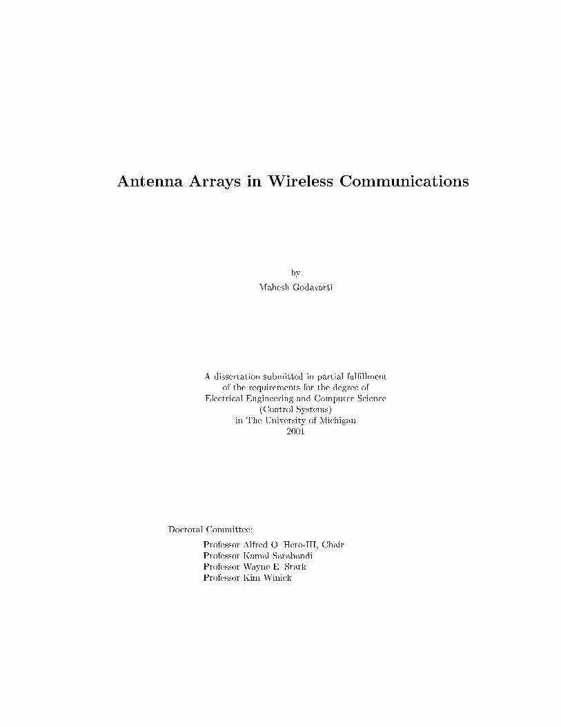
Antenna Arrays in Wireless CommunicationsbyMahesh Godavarti

A dissertation submitted in partial ful�llmentof the requirements for the degree ofElectrical Engineering and Computer Science(Control Systems)in The University of Michigan2001Doctoral Committee:Professor Alfred O. Hero-III, ChairProfessor Kamal SarabandiProfessor Wayne E. StarkProfessor Kim Winick

c Mahesh Godavarti 2001All Rights Reserved

I dedicate this work to the whole wide world.

i

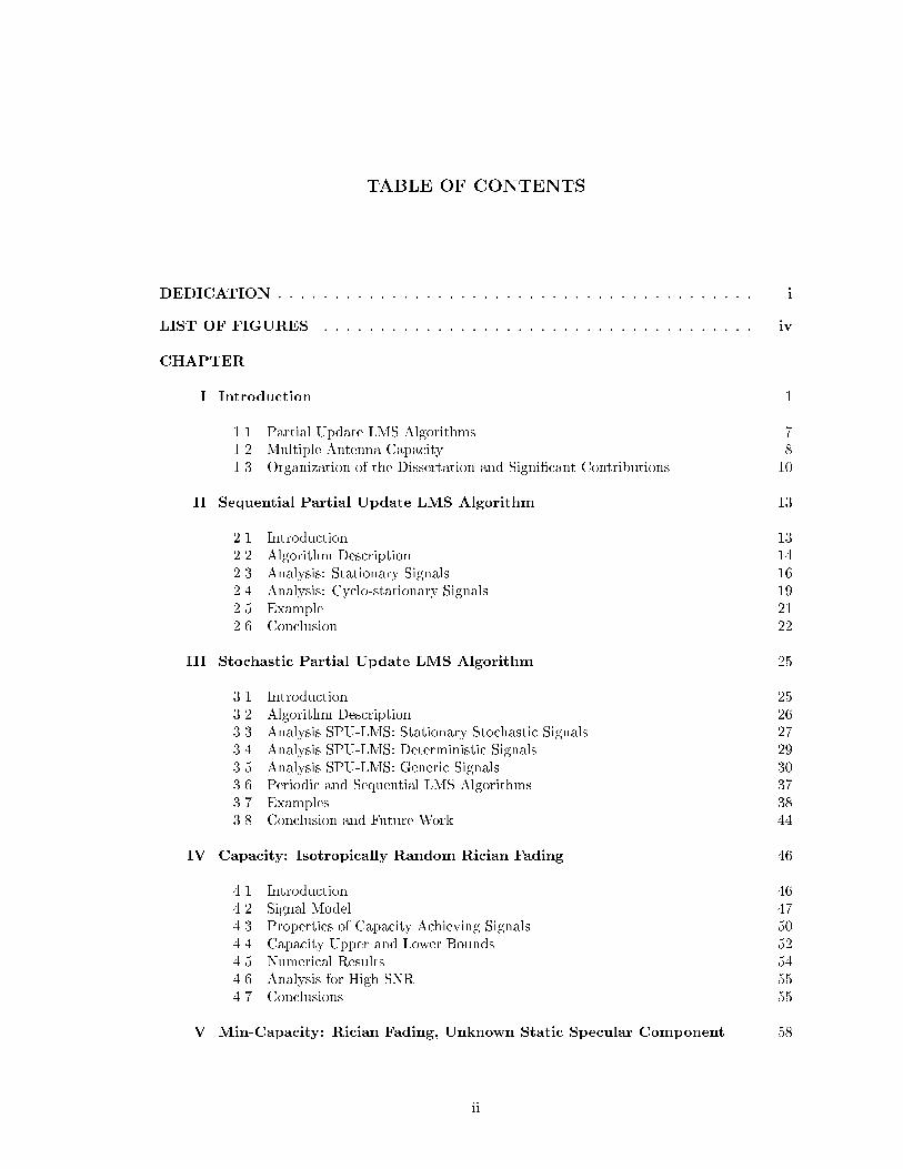
TABLE OF CONTENTSDEDICATION : : : : : : : : : : : : : : : : : : : : : : : : : : : : : : : : : : : : : : : : : : iLIST OF FIGURES : : : : : : : : : : : : : : : : : : : : : : : : : : : : : : : : : : : : : : ivCHAPTERI. Introduction . . . . . . . . . . . . . . . . . . . . . . . . . . . . . . . . . . . . . . . 11.1 Partial Update LMS Algorithms . . . . . . . . . . . . . . . . . . . . . . . . . 71.2 Multiple-Antenna Capacity . . . . . . . . . . . . . . . . . . . . . . . . . . . . 81.3 Organization of the Dissertation and Signi�cant Contributions . . . . . . . . 10II. Sequential Partial Update LMS Algorithm . . . . . . . . . . . . . . . . . . . . 132.1 Introduction . . . . . . . . . . . . . . . . . . . . . . . . . . . . . . . . . . . . 132.2 Algorithm Description . . . . . . . . . . . . . . . . . . . . . . . . . . . . . . . 142.3 Analysis: Stationary Signals . . . . . . . . . . . . . . . . . . . . . . . . . . . 162.4 Analysis: Cyclo-stationary Signals . . . . . . . . . . . . . . . . . . . . . . . . 192.5 Example . . . . . . . . . . . . . . . . . . . . . . . . . . . . . . . . . . . . . . 212.6 Conclusion . . . . . . . . . . . . . . . . . . . . . . . . . . . . . . . . . . . . . 22III. Stochastic Partial Update LMS Algorithm . . . . . . . . . . . . . . . . . . . . 253.1 Introduction . . . . . . . . . . . . . . . . . . . . . . . . . . . . . . . . . . . . 253.2 Algorithm Description . . . . . . . . . . . . . . . . . . . . . . . . . . . . . . . 263.3 Analysis SPU-LMS: Stationary Stochastic Signals . . . . . . . . . . . . . . . 273.4 Analysis SPU-LMS: Deterministic Signals . . . . . . . . . . . . . . . . . . . . 293.5 Analysis SPU-LMS: Generic Signals . . . . . . . . . . . . . . . . . . . . . . . 303.6 Periodic and Sequential LMS Algorithms . . . . . . . . . . . . . . . . . . . . 373.7 Examples . . . . . . . . . . . . . . . . . . . . . . . . . . . . . . . . . . . . . . 383.8 Conclusion and Future Work . . . . . . . . . . . . . . . . . . . . . . . . . . . 44IV. Capacity: Isotropically Random Rician Fading . . . . . . . . . . . . . . . . . 464.1 Introduction . . . . . . . . . . . . . . . . . . . . . . . . . . . . . . . . . . . . 464.2 Signal Model . . . . . . . . . . . . . . . . . . . . . . . . . . . . . . . . . . . . 474.3 Properties of Capacity Achieving Signals . . . . . . . . . . . . . . . . . . . . 504.4 Capacity Upper and Lower Bounds . . . . . . . . . . . . . . . . . . . . . . . 524.5 Numerical Results . . . . . . . . . . . . . . . . . . . . . . . . . . . . . . . . . 544.6 Analysis for High SNR . . . . . . . . . . . . . . . . . . . . . . . . . . . . . . 554.7 Conclusions . . . . . . . . . . . . . . . . . . . . . . . . . . . . . . . . . . . . 55V. Min-Capacity: Rician Fading, Unknown Static Specular Component . . . 58ii

5.1 Introduction . . . . . . . . . . . . . . . . . . . . . . . . . . . . . . . . . . . . 585.2 Signal Model and Problem Formulation . . . . . . . . . . . . . . . . . . . . . 595.3 Capacity Upper and Lower Bounds . . . . . . . . . . . . . . . . . . . . . . . 615.4 Properties of Capacity Achieving Signals . . . . . . . . . . . . . . . . . . . . 635.5 Average Capacity Criterion . . . . . . . . . . . . . . . . . . . . . . . . . . . . 665.6 Conclusions . . . . . . . . . . . . . . . . . . . . . . . . . . . . . . . . . . . . 68VI. Capacity: Rician Fading, Known Static Specular Component . . . . . . . . 696.1 Introduction . . . . . . . . . . . . . . . . . . . . . . . . . . . . . . . . . . . . 696.2 Rank-one Specular Component . . . . . . . . . . . . . . . . . . . . . . . . . . 706.3 General Rank Specular Component . . . . . . . . . . . . . . . . . . . . . . . 746.4 Training in Non-Coherent Communications . . . . . . . . . . . . . . . . . . . 896.5 Conclusions and Future Work . . . . . . . . . . . . . . . . . . . . . . . . . . 105APPENDICES : : : : : : : : : : : : : : : : : : : : : : : : : : : : : : : : : : : : : : : : : : 107.1 Derivation of Stability Condition (3.6) . . . . . . . . . . . . . . . . . . . . . 108.2 Derivation of expression (3.8) . . . . . . . . . . . . . . . . . . . . . . . . . . . 109.3 Derivation of the misadjustment factor (3.7) . . . . . . . . . . . . . . . . . . 109.4 Proof of Theorem III.1 in Section 3.5.1 . . . . . . . . . . . . . . . . . . . . . 110.5 Derivation of Expressions in Section 3.7.2 . . . . . . . . . . . . . . . . . . . . 115.6 Derivation of Expressions in Section 3.7.1 . . . . . . . . . . . . . . . . . . . . 118.7 Capacity Optimization in Section 6.2.1 . . . . . . . . . . . . . . . . . . . . . 121.8 Proof of Lemma VI.3 in Section 6.3.4 . . . . . . . . . . . . . . . . . . . . . . 123.9 Convergence of Entropies . . . . . . . . . . . . . . . . . . . . . . . . . . . . . 131.10 Convergence of H(X) for T > M = N in Section 6.3.4 . . . . . . . . . . . . . 136.11 Proof of Theorem VI.8 in Section 6.4.1 . . . . . . . . . . . . . . . . . . . . . 139.12 Proof of Theorem VI.9 in Section 6.4.1 . . . . . . . . . . . . . . . . . . . . . 140.13 Proof of Theorem VI.10 in Section 6.4.1 . . . . . . . . . . . . . . . . . . . . . 142BIBLIOGRAPHY : : : : : : : : : : : : : : : : : : : : : : : : : : : : : : : : : : : : : : : : 143

iii

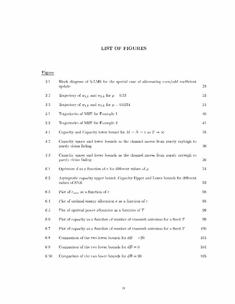
LIST OF FIGURESFigure2.1 Block diagram of S-LMS for the special case of alternating even/odd coe�cientupdate . . . . . . . . . . . . . . . . . . . . . . . . . . . . . . . . . . . . . . . . . . . 232.2 Trajectory of w1;k and w2;k for � = 0:33 . . . . . . . . . . . . . . . . . . . . . . . . 232.3 Trajectory of w1;k and w2;k for � = 0:0254 . . . . . . . . . . . . . . . . . . . . . . . 243.1 Trajectories of MSE for Example 1 . . . . . . . . . . . . . . . . . . . . . . . . . . . 403.2 Trajectories of MSE for Example 2 . . . . . . . . . . . . . . . . . . . . . . . . . . . 414.1 Capacity and Capacity lower bound for M = N = 1 as T !1 . . . . . . . . . . . 554.2 Capacity upper and lower bounds as the channel moves from purely rayleigh topurely rician fading . . . . . . . . . . . . . . . . . . . . . . . . . . . . . . . . . . . . 564.3 Capacity upper and lower bounds as the channel moves from purely rayleigh topurely rician fading . . . . . . . . . . . . . . . . . . . . . . . . . . . . . . . . . . . . 566.1 Optimum d as a function of r for di�erent values of � . . . . . . . . . . . . . . . . . 746.2 Asymptotic capacity upper bound, Capacity Upper and Lower bounds for di�erentvalues of SNR . . . . . . . . . . . . . . . . . . . . . . . . . . . . . . . . . . . . . . . 926.3 Plot of rnew as a function of r . . . . . . . . . . . . . . . . . . . . . . . . . . . . . . 986.4 Plot of optimal energy allocation � as a function of r . . . . . . . . . . . . . . . . . 986.5 Plot of optimal power allocation as a function of T . . . . . . . . . . . . . . . . . . 996.6 Plot of capacity as a function of number of transmit antennas for a �xed T . . . . 996.7 Plot of capacity as a function of number of transmit antennas for a �xed T . . . . 1006.8 Comparison of the two lower bounds for dB = �20 . . . . . . . . . . . . . . . . . . 1046.9 Comparison of the two lower bounds for dB = 0 . . . . . . . . . . . . . . . . . . . . 1046.10 Comparison of the two lower bounds for dB = 20 . . . . . . . . . . . . . . . . . . . 105

iv

CHAPTER IIntroductionWireless communications have been gaining popularity because of better antennatechnologies, lower costs, easier deployment of wireless systems, greater exibility,better reliability and need for mobile communications. In some cases, like in veryremote areas, wireless connections may be the only option.Eventhough the popularity of mobile wireless systems is a more recent phe-nomenon �xed-wireless systems have a long history. Point-to-point microwave con-nections have long been used for voice and data communications, generally in back-haul networks operated by phone companies, cable TV companies, utilities, railways,paging companies and government agencies, and will continue to be an importantpart of the communications infrastructure. Improvements in technology have allowedhigher frequencies and thus smaller antennas to be used resulting in lower costs andeasier-to-deploy systems.Another reason for the popularity of wireless systems is that o�ate consumersdemand for data rates has been insatiable. Wireline models have topped of at a rateof 56Kbps and people have been looking for ISDN and DSL connections. Companieswith T1 connections of 1.54Mbps have found the connections inadequate and areturning to T3 �ber connections. But, due to very expensive deployment of �ber1

2connections companies have been turning to �xed wireless links.This has resulted in wireless communications being found in a host of applicationsranging over �xed microwave links, wireless LANs, data over cellular networks, wire-less WANs, satellite links, digital dispatch networks, one-way and two-way pagingnetworks, di�use infrared, laser-based communications, keyless car entry, the GlobalPositioning System, mobile communications, indoor-radio and more.There is such a wide variety of research in antennas that in future [27] we can ex-pect \a hand-held terminal the size of a wristwatch capable of steering beams towarda satellite. The system would also consist of many radiating elements fabricated bymicrostrip technology, each with its own phase-shifting network, power ampli�er,and so on with other required processors manufactured by the microwave monolithicintegrated circuits technology."One challenge in wireless systems not present in wireline systems is the issue offading. Fading arises due to the possibility of multiple paths from the transmitterto the receiver with distructive combination at the receiver output. There are manymodels describing fading in wireless channels. The classic ones being rayleigh andrician at fading models. rayleigh and rician models are typically for narrowband sig-nals and don't include the doppler shift induced due to the motion of the transmitteror the receiver. For other emerging models see [18].In wireless systems, there are three di�erent ways to combat fading; 1) Frequencydiversity 2) Time diversity and 3) spatial diversity. Frequency diversity makes use ofthe fact that multipath structure for di�erent frequencies is di�erent. This fact canbe exploited to mitigate the e�ect of fading. But, the positive e�ects of frequencydiversity are limited due to bandwidth limitations. Wireless communications usesradio spectrum, a �nite resource. This limits the number of wireless users and the

3amount of spectrum available to any user at any moment in time. Time diversitymakes use of the fact that fading for di�erent time intervals is di�erent. By usingchannel coding the e�ect of bad fading intervals can be mitigated by good fadingintervals. However, due to delay constraints time diversity can't be really exploited.The third way to do it is to exploit spatial diversity using multiple antennaseither separated in space or di�erently polarized [21, 22, 47]. Di�erent antennashave di�erent multipath characteristics or di�erent fading characterisitics and thiscan be used to generate a stronger signal. Spatial diversity techniques don't have thedrawbacks associated with time diversity and frequency diversity techniques thoughspatial diversity does involve deployment of multiple antennas at the transmitter andthe receiver which is not always feasible.In this thesis, we will concentrate on spatial diversity o�ered with multiple an-tennas. Spatial diversity, receive (multiple antennas in the receiver) and transmit(multiple antennas at the transmitter), helps in improving system performance by[27]1. Improving spectrum e�ciency: Using multiple antennas we can accomodatemore than one user in a given spectral bandwidth.2. Extending range coverage: Multiple antennas can be used to direct the energyof a signal in a given direction and hence minimize unnecessary transmission ofsignal energy.3. Tracking multiple mobiles: The outputs of antennas can be combined in di�erentways to isolate signals from each and every mobile.4. Increasing channel reuse5. Reducing power usage: By directing the energy in a certain direction and in-

4creasing range coverage lesser energy can be used to reach a user at a givendistance.6. Generating multiple access: Appropriately combining the outputs of the anten-nas to selectively provide access to users.7. Increasing channel capacity: Improving spectral e�ciency allows more than oneuser to operate in a cell.8. Reducing co-channel interference9. Combating fading10. increasing information channel capacity: Multiple antennas have been used toincrease the maximum acheival data rates.Traditionally, all the gains listed above have been realized by explicitly directingthe receive or transmit antenna array to point in speci�c directions. This process iscalled beamforming. For receive antennas beamforming can be achieved electroni-cally by appropriately weighting the antenna outputs and combining them to makethe antenna response to certain directions more sensitive than others. Most of theresearch on antenna arrays for beamforming has mostly been on receivers. Transmitbeamforming is di�erent and requires di�erent algorithms and hardware [28].Di�erent kinds of beamforming at the recieve antenna array currently in use arebased on array processing algorithms such as signal copy, direction �nding and sig-nal separation algorithms [28] that include conventional beamforming, Null steeringbeamforming, Optimal beamforming, Beam-Space Processing, Blind Beamforming,Optimum Combining and Maximal Ratio combining [28, 41, 57, 2, 58, 53, 71]. Someof the beamformers require a reference signal and use adaptive algorithms like LMSto get to the optimal signal [28, 42, 69, 70].

5Adaptive algorithms can also be used for the problem of adaptive beamformingwhere it is required to track multiple users in motion or to track varying channelconditions. More popular ones [28] are the LMS Algorithm, Constant ModulusAlgorithm and the Recursive Least Squares algorithm. The algorithm of interest inthis work is the LMS Algorithm.Another research topic in the �eld of beamforming that has generated su�cientinterest involves investigating the e�ect of calibration errors in direction �nding andsignal copy problems [44, 52, 63, 62, 43, 73, 23]. An array with Gaussian calibrationerrors operating in a non-fading environment has the same model as a rician fadingchannel. Thus the work done in this thesis can be easily translated to the case ofarray calibration errors.Beamforming at the receiver is a way of exploiting receive diversity. Most of theresearch in the literature concentrates on this kind of diversity. Exploiting transmitdiversity usually involved [65] using the channel state information obtained via feed-back for reassigning energy at di�erent antennas via waterpouring, linear processingof signals to spread the information across transmit antennas and using channel codesand transmitting the codes using di�erent antennas in an orthogonal manner.The multiple transmit antennas were probably �rst used to send multiple copies ofa signal over orthogonal time or frequency slices. This of course incurs a bandwidthexpansion factor equal to the number of antennas. A transmit diversity techniquewithout bandwidth expansion was �rst suggested by Wittenben [72]. Wittenben'sdiversity technique of sending time-delayed copies of a common input signal over themultiple antennas was also independently discovered by Seshadri and Winters [60]and by Weerackody [68]. An information theoretic approach to transmit diversityschemes has been undertaken by Narula [3, 51].

6Recently, people have realized that explicit beamforming may not be the mostoptimal way to increase data rates. Foschini with his BLAST project showed thatmultipaths are not as harmuful as thought out to be and in fact can be exploited toincrease capacity. This has given rise to the concept of space-time codes [1, 65, 66,35, 34, 39, 38, 8]. Space-time coding is a coding technique that is designed for usewith multiple transmit antennas. The codes are designed in such a way to inducespatial and temporal correlations into signals that can be exploited at the receiver.Space-time codes are simply a di�erent way of looking at space-time processing ofsignals before transmission [1].Design of space-time codes has taken many forms. Tarokh et. al. [65, 66] havetaken the approach of designing space-time codes for both rayleigh and rician fadingchannels that maximizes a distance criterion. The distance criterion was derived froman upper bound on probability of decoding error. There have been code designswhere the receiver has no knowledge about the channel. Hero and Marzetta [34]design space-time codes with a design criterion of maximizing the cut-o� rate formultiple-antenna rayleigh fading channel. Hochwald et. al [35, 9] propose a designbased on signal structures that asymptotically achieve capacity in the non-coherentcase for rayleigh fading channels. Hughes [39, 38] considered the design of space-time based on the concept of Group codes. The codes can be viewed as an extendedversion of phase shift keying for the case of multiple antenna communications. In [38]the author independently proposed a scheme similar to that proposed by Hochwaldand Marzetta in [35].The research topics this disseration concentrates on are the LMS algorithm andchannel capacity of multiple antennas in the presence of rician fading. We willelaborate more on the research topics in the following sections.

71.1 Partial Update LMS AlgorithmsThe LMS algorithm is a popular algorithm for adaptation of weights in the �eldof adaptive beamforming using antenna arrays or for channel equalization to combatintersymbol interference. This has application in many areas including interferencecancellation, space time modulation and coding, signal copy in surveillance and wire-less communications. Although there are algorithms with faster convergence rateslike RLS, LMS is really popular because of ease of implementation and low compu-tational costs.One of the variants of LMS existing in literature is the Partial Update LMS Al-gorithm. Partial updating of the LMS adaptive �lter has been proposed to reducecomputational costs [46, 29, 11]. In this era of mobile computing and communi-cations, such implementations are also attractive for reducing power consumption.However, theoretical performance predictions on convergence rate and steady statetracking error are more di�cult to derive than for standard full update LMS. Accu-rate theoretical predictions are important as it has been observed that the standardLMS conditions on the step size parameter fail to ensure convergence of the partialupdate algorithm.Two of the partial update algorithms prevalent in the literature have been de-scribed in [14]. They are referred to as the \Periodic LMS algorithm" and the\Sequential LMS algorithm". To reduce computation by a factor of P , the PeriodicLMS algorithm (P-LMS) updates all the �lter coe�cients every P th iteration insteadof every iteration. The Sequential LMS (S-LMS) algorithm updates only a fractionof coe�cients every iteration.Another variant referred to as \Max Partial Update LMS algorithm" has been

8proposed in [12, 13] and [5]. In this algorithm, the subset of coe�cients to beupdated is dependent on the input signal. The subset is so chosen as to maximize thereduction in the mean squared error. The input signals multiplying each coe�cientare ordered according to their magnitude and the coe�cients corresponding to thelargest 1P of input signals are chosen for update in an iteration. Some analysis of thisalgorithm has been done in [13] for the special case of one coe�cient per iterationbut, analysis for more general cases still needs to be completed.1.2 Multiple-Antenna CapacityThe paper by Foschini et. al. [21, 22] showed that a signi�cant gain in capacitycan be achieved by using multiple antennas in the presence of rician fading. Foschiniand Telatar showed ([64]) that with perfect channel knowledge at the receiver, forhigh SNR a capacity gain of min(M;N) bits/second/Hz, where M is the number ofantennas at the transmitter and N is the number of antennas at the receiver, canbe achieved with every 3 dB increase in SNR. Channel knowledge at the receiverhowever requires that the time between di�erent fades be su�ciently large to enablethe receiver to learn the channel. This might not be true in the case of fast mobilereceivers and large numbers of transmit antennas.Following Foschini [21], there have been many papers written on the subject ofcalculating capacity for a multiple antenna channel [16, 24, 25, 47, 17, 26, 50, 31,30, 54, 48]. The most notable of these is the work done by Marzetta and Hochwald[48]. There also have been attempts to evaluate the achievable rate regions for themultiple antenna channel in terms of cut-o� rate [34] and error exponents [4].Marzetta and Hochwald [48] considered the case when neither the receiver northe transmitter has any knowledge of the fading coe�cients where the fading coef-

9�cients remain constant for T symbol periods and instantaneously change to newindependent realizations every T symbol periods. They established that to achievecapacity it is su�cient to use M = T antennas at the transmitter and the capacityachieving signal matrix consists of a product of two independent matrices, a T � Tisotropically random unitary matrix and a T �M real nonnegative diagonal matrix.Hence, it is su�cient to optimize over the density of a smaller parameter set of sizeminfM;Tg instead of the original one of size T �M .Zheng and Tse [74] derived explicit capacity results for the case of high SNR in thecase of no channel knowledge. They showed that the number of degrees of freedomfor non-coherent communication is M�(1�M�=T ) where M� = minfM;N; T=2g asopposed to minfM;Ng in the case of coherent communications.The literature cited above has limited its attention to rayleigh fading channelmodels for computing capacity of multiple-antenna wireless links. However, rayleighfading models are inadequate in describing the gamut of fading channels one comesacross in practice. Another popular model used in the literature to �ll this gap is therician fading channel. rician fading components traditionally have been modeled asindependent Gaussian components with a deterministic non-zero mean [56, 65, 49,15, 19, 59]. Farrokhi et. al. [19] used this model to analyze the capacity of a MIMOchannel with a specular component. They assume that the specular componentis deterministic and unchanging and unknown to the transmitter but, known tothe receiver. They also assume that the receiver has complete knowledge aboutthe fading coe�cients (i.e. has knowledge about the rayleigh component as well).They work with the premise that since the transmitter has no knowledge about thespecular component the signaling scheme has to be designed to guarantee a givenrate irrespective of the value of the deterministic specular component. They conclude

10that the signal matrix has to be composed of independent circular Gaussian randomvariables of mean 0 and equal variance to maximize the rate.1.3 Organization of the Dissertation and Signi�cant ContributionsIn this work, we have made signi�cant contributions in the �eld of LMS algorithmfor adaptive arrays and in evaluating shannon capacity for multiple antennas in thepresence of rician fading. The contributions in both �elds will �nd a lot of applicationin multiple-antenna wireless communications.1. In chapter II we analyze the Sequential PU-LMS for stability and come up withmore stringent conditions on stability. We validate the analysis via experimentalsimulations.� Contributions: Rigorously proved the stability of the algorithm for sta-tionary signals without restrictive assumptions and analyzed the algorithmfor cyclo-stationary signals which led to an understanding of the reasonbehind the algorithm's instability of sequential LMS algorithm. This un-derstanding led to the design of a more stable algorithm.2. chapter III contains the description of a new Partial Update Algorithm calledthe Stochastic Partial Update LMS where the coe�cients to be updated inan iteration are chosen randomly. We derive conditions for stability and alsoanalyze the algorithm for performance. We demonstrate the e�ectiveness viaexamples.� Contributions: Designed a new Partial Update algorithm with much bet-ter convergence properties than those of existing Partial Update LMS al-gorithms for the case of non-stationary signals and similar performance for

11the case of stationary signals. Also, analyzed the algorithm for di�erentscenarios including stationary signals, deterministic signals and generic sig-nals.3. In chapter IV, we use a non-traditional model where the specular component isalso modeled as random but, with an isotropically uniform density [48]. Withthis model the concept of channel capacity is clearly de�ned. We also derive alower bound to capacity.� Contributions: Proposed a new tractable model for analysis enablingcharacterization of capacity achieving signals and also derived a very usefullower bound to channel capacity which is also applicable to the case ofrayleigh fading.4. In chapter V, we use a slight variation of the traditional and well-establishedmodel where the specular component is modeled as deterministic and non-changing. The variation is that we assume the transmitter has no knowledgeabout the specular mean. In this case, the concept of channel capacity is notde�ned and we have to maximize the worst possible rate available for com-munication over the ensemble of values the unknown specular component cantake.� Contributions: Proposed a tractable formulation of the problem and de-rived capacity expressions, lower bound to capacity and characterized theproperties of capacity achieving signals.5. In chapter VI, we use the traditional and well-established model where thespecular component is modeled as deterministic and non-changing. We assumethat both the transmitter and the receiver have complete knowledge about the

12specular component. In this case, the concept of channel capacity in terms ofShannon theory is well de�ned.� Contributions: Derived coherent and non-coherent capacity expressionsin the low and high SNR regimes for a popular rician fading model. Also,showed the contrast between rician and rayleigh fading channels based oncapacity for training based communication systems.

CHAPTER IISequential Partial Update LMS Algorithm2.1 IntroductionIn [14], condition for convergence in mean for the Sequential Partial Update LMS(S-LMS) Algorithm were derived under the assumption of small step-size parameter(�) which turned out to be the same as those for the standard LMS algorithm. Thiscondition is however unreliable because of the underlying small � assumption. In thischapter, we prove without the forementioned assumption that for stationary inputsignals convergence in mean for the regular LMS algorithm guarantees convergencein mean for S-LMS.We also derive bounds on the step-size parameter � for Sequential Partial UpdateLMS (S-LMS) Algorithm which ensures convergence in mean for the special caseinvolving alternate even and odd coe�cient updates when the input signal is cyclo-stationary. The bounds are based on extremal properties of the matrix 2-norm. Wederive bounds for the case of stationary and cyclo-stationary signals. For simplicitywe make the standard independence assumptions used in the analysis of LMS [6].The organization of the chapter is as follows. First in section 2.2, a brief descrip-tion of the sequential partial update algorithm is given. The algorithm with arbitrarysequence of updates is analyzed for the case of stationary signals in section 2.3. This13

14is followed by the analysis of algorithm with the special case of alternate even andodd coe�cient updates for cyclo-stationary signals in section 2.4. In section 2.5an example is given to illustrate the usefulness of the bounds on step-size derivedin section 2.4. Finally, conclusions and directions for future work are indicated insection 2.6.2.2 Algorithm DescriptionThe block diagram of S-LMS for a N -tap LMS �lter with alternating even andodd coe�cient updates is shown in Figure 2.1It is assumed that the LMS �lter is a standard FIR �lter of even length, N . Forconvenience, we start with some de�nitions. Let fxi;kg be the input sequence andlet fwi;kg denote the coe�cients of the adaptive �lter. De�neWk = [w1;k w2;k : : : wN;k]TXk = [x1;k x2;k x3;k : : : xN;k]Twhere the terms de�ned above are for the instant k. In addition, Let dk denotethe desired response. In typical applications dk is a known training signal which istransmitted over a noisy channel with unknown FIR transfer function.In this paper we assume that dk itself obeys an FIR model given by dk =W yoptXk + nk where Wopt are the coe�cients of an FIR model given by Wopt =[w1;opt : : : wN;opt]T . Here fnkg is assumed to be a zero mean i.i.d sequence thatis independent of the input sequence Xk.For description purposes we will assume that the �lter coe�cients can be dividedinto P mutually exclusive subsets of equal size, i.e. the �lter length N is a multipleof P . For convenience, de�ne the index set S = f1; 2; : : : ; Ng. Partition S into Pmutually exclusive subsets of equal size, S1; S2; : : : ; SP . De�ne Ii by zeroing out

15the jth row of the identity matrix I if j =2 Si. In that case, IiXk will have preciselyNP non-zero entries. Let the sentence \choosing Si at iteration k" stand to mean\choosing the weights with their indices in Si for update at iteration k".The S-LMS algorithm is described as follows. At a given iteration, k, one ofthe sets Si, i = 1; : : : ; P , is chosen in a pre-determined fashion and the update isperformed. wk+1;j = 8><>: wk;j + �e�kxk;j if j 2 Siwk;j otherwise (2.1)where ek = dk�W ykXk. The above update equation can be written in a more compactform in the following mannerWk+1 = Wk + �e�kIiXk (2.2)In the special case of even and odd updates, P = 2 and S1 consists of all evenindices and S2 of all odd indices as shown in Figure 2.1.We also de�ne the coe�cient error vector asVk = Wk �Woptwhich leads to the following coe�cient error vector update for S-LMS when k is oddVk+2 = (I � �I2Xk+1Xyk+1)(I � �I1XkXyk)Vk + (2.3)�(I � �I2Xk+1Xyk+1)nkI1Xk + �nk+1I2Xk+1and the following when k is evenVk+2 = (I � �I1Xk+1Xyk+1)(I � �I2XkXyk)Vk + (2.4)�(I � �I1Xk+1Xyk+1)nkI2Xk + �nk+1I1Xk+1

162.3 Analysis: Stationary SignalsAssuming that Xk is a WSS random sequence, we analyze the convergence of themean coe�cient error vector E [Vk]. We make the standard assumptions that Vk andXk are mutually uncorrelated and that Xk is independent of Xk�1 [6] which is notan unreasonable assumption for the case of antenna arrays. For regular full updateLMS algorithm the recursion for E [Vk] is given byE [Vk+1] = (I � �R)E [Vk] (2.5)where I is the N -dimensional identity matrix and R = E hXkXyki is the input sig-nal correlation matrix. The necessary and su�cient condition for stability of therecursion is given by 0 < � < 2=�max (2.6)where �max is the maximum eigen-value of the input signal correlation matrix R.Taking expectations under the same assumptions as above, using the independenceassumption on the sequences Xk; nk, the mutual independence assumption onXk andVk, and simplifying we obtain for odd k when S-LMS is operating under the specialcase of alternate even and odd updatesE [Vk+2] = (I � �I2R)(I � �I1R)E[Vk] (2.7)and for even k E [Vk+2] = (I � �I1R)(I � �I2R)E[Vk] (2.8)It can be shown that under the above assumptions on Xk; Vk and dk, the convergenceconditions for even and odd update equations are identical. We therefore focus on(2.7). Now to ensure stability of (2.7), the eigenvalues of (I��I2R)(I��I1R) should

17lie inside the unit circle. We will show that if the eigenvalues of I��R lie inside theunit circle then so do the eigenvalues of (I � �I2R)(I � �I1R).Now, if instead of just two partitions of even and odd coe�cients (P = 2) wehave any number of arbitrary partitions (P � 2) then the update equations can besimilarly written as above with P > 2. Namely,E[Vk+P ] = PYi=1(I � �IiR)E[Vk] (2.9)We will show that for any arbitrary partition of any size (P � 2); S-LMS convergesin the mean if LMS converges in the mean(Theorem II.2). The case P = 2 followsas a special case.We will show that if R is a positive de�nite matrix of dimension N � N witheigenvalues lying in the open interval (0; 2) thenQPi=1(I�IiR) has eigenvalues insidethe unit circle. Ii, i = 1; : : : ; P is obtained from I, the identity matrix of dimensionN �N , by zeroing out some rows in I such that PMi=1 Ii is positive de�nite.The following theorem is used in proving the main result in Theorem II.2.Theorem II.1. [36, Prob. 16, page 410] Let B be an arbitrary N � N matrix.Then �(B) < 1 if and only if there exists some positive de�nite N � N matrixA such that A � ByAB is positive de�nite. �(B) denotes the spectral radius of B(�(B) = max1;::: ;N j�i(B)j).Theorem II.2. Let R be a positive de�nite matrix of dimension N�N with �(R) =�max(R) < 2 then �(QPi=1(I�IiR)) < 1 where Ii, i = 1; : : : ; P are obtained by zeroingout some rows in the identity matrix I such that PPi=1 Ii is positive de�nite. ThusS-LMS converges in the mean if LMS converges in the mean.Proof: Let x0 2 Cl N be an arbitrary non-zero vector of length N . Let xi =(I � IiR)xi�1. Also, let P =QPi=1(I � IiR).

18First we will show that xyiRxi � xyi�1Rxi�1 � �xyi�1RIiRxi�1, where � = 12(2 ��max(R)) > 0. xyiRxi = xyi�1(I � RIi)R(I � IiR)xi�1= xyi�1Rxi�1 � �xyi�1RIiRxi�1 ��xyi�1RIiRxi�1 + xyi�1RIiRIiRxi�1where � = 2� �. If we can show �RIiR�RIiRIiR is positive semi-de�nite then weare done. Now �RIiR� RIiRIiR = �RIi(I � 1�R)IiRSince � = (1+�max(R)=2) > �max(R) it is easy to see that I� 1�R is positive de�nite.Therefore, �RI1R� RI1RI1R is positive semi-de�nite andxyiRxi � xyi�1Rxi�1 � �xyi�1RIiRxi�1Combining the above inequality for i = 1; : : : ; P , we note that xyPRxP < xy0Rx0if xyi�1RIiRxi�1 > 0 for at least one i, i = 1; : : : ; P . We will show by contradictionthat is indeed the case.Suppose not, then xyi�1RIiRxi�1 = 0 for all i, i = 1; : : : ; P . Since, xy0RI1Rx0 = 0this implies I1Rx0 = 0. Therefore, x1 = (I � I1R)x0 = x0. Similarly, xi = x0 forall i, i = 1; : : : ; P . This in turn implies that xy0RIiRx0 = 0 for all i, i = 1; : : : ; Pwhich is a contradiction since R(PPi=1 Ii)R is a positive-de�nite matrix and 0 =PPi=1 xy0RIiRx0 = xy0R(PPi=1 Ii)Rx0 6= 0.Finally, we conclude that xy0PyRPx0 = xyPRxP< xy0Rx0

19Since x0 is arbitrary we have R � PyRP to be positive de�nite so that applyingTheorem II.1 we conclude that �(P) < 1.Finally, if LMS converges in the mean we have �(I � �R) < 1 or �max(�R) < 2.Which from the above proof is su�cient for concluding that �(QPi=1(I � �IiR)) < 1.Therefore, S-LMS also converges in the mean.2.4 Analysis: Cyclo-stationary SignalsNext, we consider the case when Xk is cyclo-stationary. We limit our attentionto S-LMS with alternate even and odd updates as shown in Figure 2.1. Let Xk be acyclo-stationary signal with period L. i.e, Ri+L = Ri. For simplicity, we will assumeL is even. For the regular LMS algorithm we have the following L update equationsE [Vk+L] = L�1Yi=0 (I � �Ri+d)E [Vk] (2.10)for d = 1; 2; : : : ; L, in which case we would obtain the following su�cient conditionfor convergence 0 < � < mini f2=�i;maxg (2.11)where �i;max is the largest eigenvalue of the matrix Ri.De�ne Ak = (I � �I1Rk) and Bk = (I � �I2Rk) then for the partial updatealgorithm the 2L valid update equations areE [Vk+L] = 0@L�12Yi=0 B2�i+1+dA2�i+d1AE [Vk] (2.12)for d = 1; 2; : : : ; L andE [Vk+L] = 0@L�12Yi=0 A2�i+1+dB2�i+d1AE [Vk] (2.13)for d = 1; 2; : : : ; L.

20Let kAk denote the spectral norm �max(AAy) of the matrix A. Then for ensuringthe convergence of the iteration (2.12) and (2.13) a su�cient condition iskBi+1Aik < 1 and kAi+1Bik < 1 for i = 1; 2; : : : ; L (2.14)Since we can write Bi+1Ai asBi+1Ai = (I � �Ri) + �I2(Ri � Ri+1) + �2I2Ri+1I1Ri (2.15)and Ai+1Bi asAi+1Bi = (I � �Ri) + �I1(Ri � Ri+1) + �2I1Ri+1I2Ri (2.16)we have the the following expression which upper bounds both kBi+1Aik and kAi+1BikkI � �Rik+ �kRi+1 � Rik+ �2kRi+1kkRik (2.17)This tells us that the su�cient condition to ensure convergence of both (2.12) and(2.13) is kI � �Rik+ �kRi+1 � Rik+ �2kRi+1kkRik < 1 (2.18)for i = 1; : : : ; L.If we make the assumption that� < mini f 2�i;max + �i;mingand �i = kRi+1 �Rik < maxf�i;min; �i+1;ming = �ifor i = 1; 2; : : : ; L then (2.18) translates to1� ��i + ��i + �2�i;max�i+1;max < 1 (2.19)

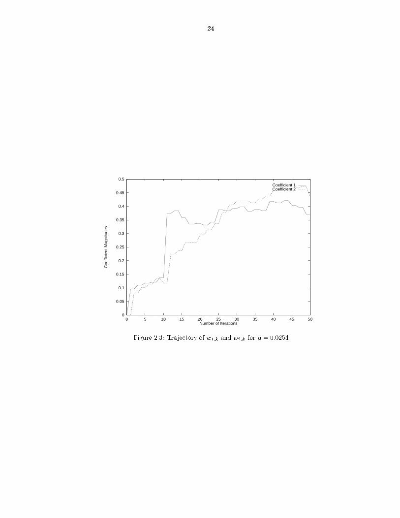
21which gives 0 < � < Lmini=1 f �i � �i�i;max�i+1;max g (2.20)(2.20) is the su�cient condition for the convergence of S-LMS.2.5 ExampleThe usefulness of the bound on step-size for the cyclo-stationary case can begauged from the following example. Consider a 2-tap �lter and a cyclo-stationaryfxi;k = xk�i+1g with period 2 having the following auto-correlation matricesR1 = 264 5:1354 �0:5733� 0:6381i�0:5733 + 0:6381i 3:8022 375R2 = 264 3:8022 1:3533 + 0:3280i1:3533� 0:3280i 5:1354 375For this choice of R1 and R2 �1 and �2 turn out to be 3:38 and we have kR1�R2k =2:5343 < 3:38. Therefore, R1 and R2 satisfy the assumption made for analysis. Now,� = 0:33 satis�es the condition for the regular LMS algorithm but, the eigenvaluesof B2A1 for this value of � have magnitudes 1:0481 and 0:4605. Since one of theeigenvalues lies outside the unit circle (2.12) is unstable for this choice of �. Whereas (2.20) gives � = 0:0254. For this choice of � the eigenvalues of B2A1 turn out tohave magnitudes 0:8620 and 0:8773. Hence (2.12) is stable.We have plotted the evolution trajectory of the 2-tap �lter with input signalsatisfying the above properties. We chose Wopt = [0:4 0:5] in Figures 2.2 and 2.3.For Figure 2.2 � was chosen according to be 0:33 and for Figure 2.3 � was chosen tobe 0:0254. For simulation purposes we set dk =W yoptSk+nk where Sk = [sk sk�1]� is avector composed of the cyclo-stationary process fskg with correlation matrices given

22as above, and fnkg is a white sequence, with variance equal to 0:01, independent offskg. We set fxkg = fskg+fvkg where fvkg is a white sequence, with variance equalto 0:01, independent of fskg.2.6 ConclusionWe have analyzed the alternating odd/even partial update LMS algorithm and wehave derived stability bounds on step-size parameter � for wide sense stationary andcyclo-stationary signals based on extremal properties of the matrix 2-norm. For thecase of wide sense stationary signals we have shown that if the regular LMS algorithmconverges in mean then so does the sequential LMS algorithm for the general caseof arbitrary but �xed ordering of the sequence of partial coe�cient updates. Forcyclo-stationary signals the bounds derived may not be the weakest possible boundsbut they do provide the user with a useful su�cient condition on � which ensuresconvergence in the mean. We believe the analysis undertaken in this paper is the�rst step towards deriving concrete bounds on step-size without making small �assumptions. The analysis also leads directly to an estimate of mean convergencerate.In the future, it would be useful to analyze partial update algorithm, without theassumption of independent snapshots and also, if possible, perform a second orderanalysis (mean square convergence). Furthermore, as S-LMS exhibits poor conver-gence in non-stationary signal scenarios (illustrative example given in the followingchapter) it is of interest to develop new partial update algorithms with better con-vergence properties. One such algorithm based on randomized partial updating of�lter coe�cients is described in the following chapter (chapter III).

23

w wL,kw1,k 3,k

k-L+1xk-L+2 xk-L+3xk-1 xk-2

L-1,kw

x

w2,k

xk

L-2,kw

dd

e

^ k

k

k

+ ++

++

+ + + + + +-

LEGEND:

Sequential Partial Update LMS Algorithm

: Set of odd weight vectors (W

: Set of even weight vectors (W

: X

: X

: Update when k odd

: Update when k even

o,k

e,k

)o,k)e,k

Figure 2.1: Block diagram of S-LMS for the special case of alternating even/odd coe�cient update

0

2000

4000

6000

8000

10000

12000

0 5 10 15 20 25 30 35 40 45 50

Coe

ffici

ent M

agni

tude

s

Number of Iterations

Coefficient 1Coefficient 2

Figure 2.2: Trajectory of w1;k and w2;k for � = 0:33

24

0

0.05

0.1

0.15

0.2

0.25

0.3

0.35

0.4

0.45

0.5

0 5 10 15 20 25 30 35 40 45 50

Coe

ffici

ent M

agni

tude

s

Number of Iterations

Coefficient 1Coefficient 2

Figure 2.3: Trajectory of w1;k and w2;k for � = 0:0254

CHAPTER IIIStochastic Partial Update LMS Algorithm3.1 IntroductionThe important characteristic of the partial update algorithms described in section1.1 is that the coe�cients to be updated at an iteration are pre-determined. It is thischaracteristic which renders P-LMS (see 1.1) and S-LMS unstable for certain signalsand which makes random coe�cient updating attractive. The algorithm proposedin this chapter is similar to S-LMS except that the subset of the �lter coe�cientsthat are updated each iteration is selected at random. The algorithm, referred toas Stochastic Partial Update LMS algorithm (SPU-LMS), involves selection of asubset of size NP coe�cients out of P possible subsets from a �xed partition of the Ncoe�cients in the weight vector. For example, �lter coe�cients can be partitionedinto even and odd subsets and either even or odd coe�cients are randomly selectedto be updated in each iteration. In this chapter we derive conditions on the step-sizeparameter which ensures convergence in the mean and the mean square sense forstationary signals, generic signals and deterministic signals.The organization of the chapter is as follows. First, a brief description of thealgorithm is given in section 3.2 followed by analysis of the stochastic partial updatealgorithm for the stationary stochastic signals in section 3.3, deterministic signals in25

26section 3.4 and for generic signals in 3.5. section 3.6 gives a description of of theexisting Partial Update LMS algorithms. This is followed by section 3.7 consistingof examples where in section 3.7.1 veri�cation of theoretical analysis of the newalgorithm is carried out via simulations and examples are given to illustrate theusefulness of SPU-LMS. In sections 3.7.2 and 3.7.3 techniques developed in section3.5 are used to show that the performance of SPU-LMS is very close to that of LMSin terms of �nal misconvergence. Finally conclusions and directions for future workare indicated in section 3.8.3.2 Algorithm DescriptionUnlike in the standard LMS algorithm where all the �lters taps are updated everyiteration the algorithm proposed in this chapter updates only a subset of coe�cientsat each iteration. The subset to be updated is chosen in a random manner so thateventually every weight is updated.The description of SPU-LMS is very similar to that of S-LMS (section 2.2). Theonly di�erence is as as follows. At a given iteration, k, for S-LMS one of the setsSi, i = 1; : : : ; P is chosen in a pre-determined fashion whereas for SPU-LMS, one ofthe sets Si is chosen at random from fS1; S2; : : : ; SPg with probability 1P and theupdate is performed. i.e.wk+1;j = 8><>: wk;j + �e�kxk;j if j 2 Siwk;j otherwise (3.1)where ek = dk�W ykXk. The above update equation can be written in a more compactform in the following mannerWk+1 = Wk + �e�kIiXk (3.2)where Ii now is a randomly chosen matrix.

273.3 Analysis SPU-LMS: Stationary Stochastic SignalsIn the stationary signal setting the o�ine problem is to choose an optimalW suchthat �(W ) = E [(dk � yk)(dk � yk)�]= E �(dk �W yXk)(dk �W yXk)��is minimized, where a� denotes the complex conjugate of a. The solution to thisproblem is given by Wopt = R�1r (3.3)where R = E[XkXyk] and r = E[d�kXk]. The minimum attainable �(W ) is given by�min = E[dkd�k]� ryR�1rFor the following analysis, we assume that the desired signal, dk satis�es the followingrelation dk =W yoptXk + nk (3.4)where Xk is a zero mean circular Gaussian random vector and nk is a zero meancircular complex Gaussian (not necessarily white) noise, with variance �min, uncor-related with Xk. It can be easily veri�ed that the model assumed for dk is same asassuming dk and Xk are jointly zero mean complex circular Gaussian sequences.We also make the independence assumption used in the analysis of standard LMS[6] which is reasonable for the present application of adaptive beamforming. Weassume that Xk is a Gaussian random vector and that Xk is independent of Xj forj < k. We also assume that Ii and Xk are mutually independent.

28For convergence-in-mean analysis we obtain the following update equation condi-tioned on a choice of Si.E[Vk+1jSi] = (I � �IiR)E[VkjSi]which after averaging over all choices of Si givesE[Vk+1] = (I � �P R)E[Vk]To obtain the above equation we have made use of the fact that the choice of Si isindependent of Vk and Xk. Therefore, � has to satisfy 0 < � < 2P�max to guaranteeconvergence in mean.For convergence-in-mean square analysis we are interested in the convergence ofE[eke�k]. Under the assumptions we obtain E[eke�k] = �min + trfRE[VkV yk ]g where�min is as de�ned earlier.We have followed the procedure of [37] for our mean-square analysis. First, condi-tioned on a choice of Si, the evolution equation of interest for trfRE[VkV yk ]g is givenby RE[Vk+1V yk+1jSi] = RE[VkV yk jSi]� 2�RIiRE[VkV yk jSi] +�2IiRIiE[XkXykAkXkXykjSi] + �2�minRIiRIiwhere Ak = E[VkV yk ]. For simplicity, consider the case of block diagonal R satisfyingPPi=1 IiRIi = R. Then, we obtain the �nal equation of interest for convergence-in-mean square to beGk+1 = (I � 2�P �+ �2P �2 + �2P �211� )Gk + �2P �min�21 (3.5)where Gk is a vector of diagonal elements of �E[UkU yk ] where Uk = QVk with Q suchthat QRQy = �. It is easy to obtain the following necessary and su�cient conditions

29(see Appendix .1) for convergence of the SPU-LMS algorithm0 < � < 2�max (3.6)�(�) def= PNi=1 ��i2���i < 1which is independent of P and identical to that of LMS.We used the integrated MSE di�erence J =P1k=0[�k� �1] introduced in [20] as ameasure of the convergence rate andM(�) = �1��min�min as a measure of misadjustment.The misadjustment factor is simply (see Appendix .3)M(�) = �(�)1� �(�) (3.7)which is same as that of the standard LMS. Thus, we conclude that random updateof subsets has no e�ect on the �nal excess mean-squared error.Finally, it is straightforward to show (see Appendix .2) the integrated MSE dif-ference is J = P trf[2��� �2�2 � �2�211� ]�1(G0 �G1)g (3.8)which is P times the quantity obtained for standard LMS algorithm. Therefore, weconclude that for block diagonal R, random updating slows down convergence bya factor of P without a�ecting the misadjustment. Furthermore, it can be easilyveri�ed that 0 < � < 1trfRg is a su�cient region for convergence of SPU-LMS andthe standard LMS algorithm.3.4 Analysis SPU-LMS: Deterministic SignalsHere we followed the analysis given in [61, pp. 140{143] which can be extendedto SPU-LMS with complex signals in a straightforward manner. We assume thatthe input signal Xk is bounded, that is supk(XykXk) � B <1 and that the desired

30signal dk follows the model dk = W yoptXkDe�ne Vk = Wk �Wopt and ek = dk �W ykXk. Then we can show that if � < 2=Bthen e2k ! 0 as k !1, and if in addition the signal satis�es the following persistenceof excitation condition:for all k, there exist K <1, �1 > 0 and �2 > 0 such that�1I < k+KXi=k XiXyi < �2I (3.9)then VkyVk ! 0 exponentially fast and V yk Vk ! 0 at a rate o( 1k ). Here, f�g indi-cates statistical expectation over all possible choices of Si, where each Si is chosenuniformly from fS1; : : : ; SPg.Condition (3.9) is identical to the persistence of excitation condition for standardLMS. Therefore, the su�cient condition for exponential stability of LMS is enoughto guarantee asymptotic stability of SPU-LMS.3.5 Analysis SPU-LMS: Generic SignalsIn this section, we analytically compare the performance of LMS and SPU-LMS interms of stability and misconvergence when the independent snapshots assumptionis invalid. For this we employ the theory developed in [45] and [55]. Eventhough thetheory developed is for the case of real random variables it can easily be adapted tothe case of complex circular random variables.In this section, results for stability and performance for the case of SPU-LMS aredeveloped for describing the performance hit taken when going from LMS to SPU-LMS. One of the important results obtained is that for stability we establish that

31LMS and SPU-LMS have the same necessary and su�cient conditions. The theoryused for stability analysis and performance analysis is from [45] and [55], respectively.3.5.1 Stability AnalysisNotations and De�nitionsNotations are the same as those used in [45]. kXkp is used to denote the Lp-norm of a random matrix X given as kXkp def= fEkXkpk1=p for p � 1 wherekXk def= fPi;j jxj2ijg1=2 is the Euclidean norm of the matrix X. Note that in [45],kXk def= f�max(XXy)g1=2. Since the two norms are related by a constant the resultsin [45] could as well have been stated with the de�nition used here. We use thisde�nition since this is the one used in [55].A process Xk is said to be �-mixing if there is a function �(m) such that �(m)! 0as m!1 andsupA2Mk�1(X);B2M1k+m(X)jP (BjA)� P (B)j � �(m); 8m � 0; k 2 (�1;1)where Mji (X), �1 � i � j � 1 is the �-algebra generated by fXkg, i � k � jFor any random matrix sequence F = fFkg, de�ne Sp(�; ��) for �� > 0 and0 < � < 1=�� bySp(�; ��) = 8<:F : kYj=i+1(I � �Fj) p � K�;��(F )(1� ��)k�i8� 2 (0; ��]; 8k � i � 0gBasically, Sp(�; ��) is the family of Lp-stable random matrices.Similarly, the averaged exponentially stable family is de�ned as S(�; ��) for �� > 0and 0 < � < 1=�� byS(�; ��) = 8<:F : kYj=i+1(I � �E[Fj]) p � K�;��(E[F ])(1� ��)k�i (3.10)8� 2 (0; ��]; 8k � i � 0g

32We also de�ne Sp and S as Sp def= [��2(0;1) [�2(0;1=��)Sp(�; ��) and S def= [��2(0;1)[�2(0;1=��)S(�; ��).ResultsLet Xk be the input signal vector generated from the following processXk = 1Xj=�1A(k; j)�k�j + k (3.11)with P1j=�1 supk kA(k; j)k < 1. f kg is a d-dimensional deterministic process,and f�kg is a general m-dimensional �-mixing sequence. The weighting matricesA(k; j) 2 Rd�m are assumed to be deterministic.We prove the following theorem which is similar to Theorem 2 in [45].Theorem III.1. Let Xk be as de�ned above with f�kg a �-mixing sequence such thatit satis�es for any n � 1 and any integer sequence j1 < j2 : : : jnE "exp � nXi=1 k�jik2!# �M exp(Kn) (3.12)where �, M , and K are positive constants. Then for any p � 1, there exist constants�� > 0, M > 0, and � 2 (0; 1) such that for all � 2 (0; ��] and for all t � k � 0"E tYj=k+1(I � �IjXjXyj ) p#1=p � M(1� ��)t�kwhere Ij is a sequence of i.i.d d� d masking matrices, if and only if there exists aninteger h > 0 and a constant � > 0 such that for all k � 0k+hXi=k+1E[XiXyi ] � �I (3.13)Proof: For proof see Appendix .4.Note that the LMS algorithm has the same necessary and su�cient condition forconvergence. Therefore, SPU-LMS behaves exactly like LMS in this respect.

333.5.2 Performance AnalysisFor perforance analysis, we assume thatdk = XykWopt;k + nkWopt;k varies as follows Wopt;k+1 �Wopt;k = wk+1, where wk+1 is the lag noise. Thenfor LMS we can write the evolution equation for the tracking error Vk def= Wk�Wopt;kas Vk+1 = (I � �XkXyk)Vk + �Xknk � wk+1and for SPU-LMS the corresponding equation can be written asVk+1 = (I � �IkXkXyk)Vk + �Xknk � wk+1In the example used in this report it is assumed that wk = 0 for all k.Now, Vk+1 can be decomposed [55] as Vk+1 = uVk + �nVk + wVk whereuVk+1 = (I � �PkXkXyk)uVk uV0 = V0 = �Wopt;0nVk+1 = (I � �PkXkXyk)nVk + PkXknk nV0 = 0wVk+1 = (I � �PkXkXyk)wVk � wk+1 nV0 = 0where Pk = I for LMS and Pk = Ik for SPU-LMS. fuVkg denotes the transientterm, re ecting the way the successive estimates of the regression coe�cients forgetthe initial conditions. fnVkg accounts for the errors introduced by the measurementnoise, nk and fvVkg accounts for the errors associated with the lag-noise fwkg.So, in general nVk and wVk obey the following inhomogenous equation�k+1 = (I � �Fk)�k + �k; �0 = 0

34�k can be represent by a set of recursive equations as follows�k = J (0)k + J (1)k + : : :+ J (n)k +H(n)kwhere the processes J (r)k ; 0 � r < n and H(n)k are described byJ (0)k+1 = (I � � �Fk)J (0)k + �k; J (0)0 = 0J (r)k+1 = (I � � �Fk)J (r)k + �ZkJ (r�1)k ; J (r)k = 0; 0 � k < rH(n)k+1 = (I � �Fk)H(n)k + �ZkJ (n)k ; H(n)k = 0; 0 � k < nwhere �Fk is an appropriate deterministic process. It usually is chosen as �Fk = E[Fk].In [55] under appropriate conditions it was shown that there exists some constantC <1 and �0 > 0 such that for all 0 < � � �0, we havesupk�0 kH(n)k kp � C�n=2Notations and De�nitionsNow, we modify the de�nition of weak dependence as given in [55] for circularcomplex random variables. The theory developed in [55] can be easily adapted forcircular random variables using this de�nition. Let q � 1 and X = fXngn�0 be a(l � 1) matrix valued process. Let � = (�(r))r2N be a sequence of positive numbersdecreasing to zero at in�nity. The complex process X = fXngn�0 is said to be (�; q)-weak dependent if there exist �nite constants C = fC1; : : : ; Cqg, such that for any1 � m < s � q and m-tuple k1; : : : ; km and any (s � m)-tuple km+1; : : : ; ks, withk1 � : : : � km < km + r � km+1 � : : : � ks, it holds thatsup1�i1;::: ;is�l;fk1;i1 ;fk2;i2 :::fkm;im ���cov �fk1;i1( ~Xk1;i1) � : : : � fkm;im( ~Xkm;im);fkm+1;im+1( ~Xkm+1;im+1) � : : : � fks;is( ~Xks;is)���� � Cs�(r)

35where ~Xn;i denotes the i-th component of Xn�E(Xn) and the set of functions fn;i()that the sup is being taken over are given by fn;i( ~Xn;i) = ~Xn;i and fn;i( ~Xn;i) = ~X�n;i.De�ne N (p) from [55] as followsN (p) = n� : Ptk=sDk�k p � �p(�) �Ptk=s jDkj2�1=2 80 � s � tand 8D = fDkgk2N(q � l) deterministic matrices gFk can be written as Fk = PkXkXyk where Pk = I for LMS and Pk = Ik for SPU-LMS. It is assumed that the following hold true for Fk. For some r; q 2 N , �0 > 0and 0 < � < 1=�0� F1(r; �; �0) fFkgk�0 is in S(r; �; �0) that is fFkg is Lr-exponentially stable.� F2(�; �0) fE[Fk]gk�0 is in S(�; �0), that is fE[Fk]gk�0 is averaged exponentiallystable.Conditions F3 and F4 stated below are trivially satis�ed for Pk = I and Pk = Ik.� F3(q; �0) supk2N sup�2(0;�0] kPkkq <1 and supk2N sup�2(0;�0] jE[Pk]j <1� F4(q; �0) supk2N sup�2(0;�0] ��1=2kPk � E[Pk]kq <1The excitation sequence � = f�kkk�0 [55] is assumed to be decomposed as �k =Mk�k where the processes M = fMkgk�0 is a d � l matrix valued process and � =f�kgk�0 is a (l � 1) vector-valued process that veri�es the following assumptions� EXC1 fMkgk2Z is Mk0(X)-adapted and Mk0(�) and Mk0(X) are independent.� EXC2(r; �0), (r > 0; �0 > 0) sup�2(0;�0 ] supk�0 kMkkr <1� EXC3(p; �0), (p > 0; �0 > 0) � = f�kgk2N belongs to N (p).

36ResultsThe following theorems from [55] are relevant.Theorem III.2 (Theorem 1 in [55]). Let n 2 N and let q � p � 2. AssumeEXC1, EXC2(pq=(q�p); �0) and EXC3(p; �0). For a; b; � > 0, a�1+ b�1 = 1, andsome �0 > 0, assume in addition F2(�; �0), F4(aqn; �0) and� fGkgk�0 is (�; (q + 2)n) weakly dependent and P(r + 1)((q+2)n=2)�1�(r) <1� supk�0 kGkkbqn <1Then, there exists a constant K < 1 (depending on �(k), k � 0 and on thenumerical constants p; q; n; q; b; �0; � but not otherwise on fXkg, f�kg or on �), suchthat for all 0 < � � �0, for all 0 � r � nsups�1 kJ (r)s kp � K�p(�) supk�0 kMkkpq=(q�p)�(r�1)=2Theorem III.3 (Theorem 2 in [55]). Let p � 2 and let a; b; c > 0 such that 1=a+1=b+ 1=c = 1=p. Let n 2 N . Assume F1(a; �; �0) and� sups�0 kZskb <1� sups�0 kJ (n+1)s kc <1Then there exists a constant K 0 <1 (depending on the numerical constants a; b; c; �; �0; nbut not on the process f�kg or on the stepsize parameter �), such that for all 0 <� � �0, sups�0 kH(n)s kp � K 0 sups�0 kJ (n+1)s kcIt is shown that if LMS satis�es the assumptions above (assumptions in section 3.2in [55]) then so does SPU-LMS. Conditions F1 and F2 follow directly from TheoremIII.1. It is easy to see that F3 and F4 hold easily for LMS and SPU-LMS.

37Lemma III.1. The constants in Theorem III.2 calculated for LMS can also be usedfor SPU-LMS.Proof: Here all that is needed to be shown is that if LMS satis�es the condi-tions (EXC1), (EXC2) and (EXC3) then so does SPU-LMS. Moreover, the upperbounds on the norms for LMS are also upper bounds for SPU-LMS. That easily fol-lows because MLMSk = Xk whereas MSPU�LMSk = IkXk and kIkk � 1 for any normk � k.Lemma III.2. The constants in Theorem III.3 calculated for LMS can also be usedfor SPU-LMS.Proof: First we show that if for LMS sups�0 kZskb < 1 then so it is for SPU-LMS. First, note that for LMS we can write ZLMSs = XsXys � E[XsXys ] whereas forSPU-LMSZSPU�LMSs = IsXsXys � 1P E[XsXys ] = IsXsXys � IsE[XsXys ] + (Is � 1P I)E[XsXys ]That means kZSPU�LMSs kb � kIskbkZLMSs kb + kIs � 1P IkbkE[XsXys ]kb. Therefore,since sups�0 kbE[XsXys ]kb <1 and sups�0 kZLMSs kb <1we have sups kZSPU�LMSs kb <1. Since all conditions for Theorem 2 have been satis�ed by SPU-LMS in a similarmanner the constants obtained are also the same.The two lemmas states that the error terms are bounded above by same constants.3.6 Periodic and Sequential LMS AlgorithmsFor P-LMS, the update equation can be written as followsWk+P =Wk + �ekXkFor the Sequential LMS algorithm the update equation is same as (3.2) except thatthe choice of Ii is no longer random. The sequence of Ii as k progresses is pre-

38determined and �xed.For the P-LMS algorithm, using the method of analysis described in [37] weconclude that the conditions for convergence are identical to standard LMS. That is(3.6) holds also for P-LMS. Also, the misadjustment factor remains the same. Theonly di�erence between LMS and P-LMS is that the measure J for P-LMS is Ptimes that of LMS. Therefore, we see that the behavior of SPU-LMS and P-LMSalgorithms is very similar for stationary signals.The di�erence between P-LMS and SPU-LMS becomes evident for deterministicsignals. From the persistence of excitation condition shown in [14] for P-LMS weconclude that the condition is stricter for P-LMS than for SPU-LMS. In fact, in thenext section we construct signals for which P-LMS is guaranteed not to convergewhereas SPU-LMS will converge.The convergence of Sequential LMS algorithm has been analyzed using the small� assumption in [14]. Theoretical results for this algorithm are not presented here.It is only shown through examples that this algorithm diverges for certain kind ofsignals and therefore should be employed with caution.3.7 Examples3.7.1 Illustration of Utility of SPU-LMSWe simulated an m-element uniform linear antenna array operating in a multiplesignal environment. Let Ai denote the response of the array to the ith plane wavesignal: Ai = [e�j(m2 � ~m)!i e�j(m2 �1� ~m)!i : : : ej(m2 �1� ~m)!i ej(m2 � ~m)!i]� where ~m = (m +1)=2 and !i = 2�D sin �i� , i = 1; : : : ;M . �i is the broadside angle of the ith signal,D is the inter-element spacing between the antenna elements and � is the commonwavelength of the narrowband signals in the same units as D and 2�D� = 2. Thearray output at the kth snapshot is given by Xk =PMi=1Aisk;i+nk where M denotes

39the number of signals, the sequence fsk;ig the amplitude of the ith signal and nk thenoise present at the array output at the kth snapshot. The objective, in both theexamples, is to maximize the SNR at the output of the beamformer. Since the signalamplitudes are random the objective translates to obtaining the best estimate ofsk;1, the amplitude of the desired signal, in the MMSE sense. Therefore, the desiredsignal is chosen as dk = sk;1.In the �rst example, the array has 4 elements and a single planar waveform withamplitude, sk;1 propagates across the array from direction angle, �1 = �2 . The am-plitude sequence fsk;1g is a BPSK signal with period four taking values on f�1; 1gwith equal probability. The additive noise nk is circular Gaussian with variance 0:25and mean 0. In all the simulations for SPU-LMS, P-LMS, and S-LMS the number ofsubsets for partial updating, P was chosen to be 4. It can be easily determined from(3.6) that for Gaussian and independent signals the necessary and su�cient conditionfor convergence of LMS and SPU-LMS is � < 0:67. Figure 3.1 shows representativetrajectories of the empirical mean-squared error for LMS, SPU-LMS, P-LMS andS-LMS algorithms averaged over 100 trials for � = 0:6 and � = 1:0. All algorithmswere found to be stable for the BPSK signals even for � values greater than 0:67.It was only as � approached 1 that divergent behavior was observed. As expected,LMS and SPU-LMS were observed to have similar � regions of convergence. It isalso clear from Figure 3.1, that as, expected SPU-LMS, P-LMS, and S-LMS takeroughly 4 times longer to converge than LMS.In the second example, we consider an 8-element uniform linear antenna arraywith one signal of interest propagating at angle �1 and 3 interferers propagating atangles �i, i = 2; 3; 4. The array noise nk is again mean 0 circular Gaussian but withvariance 0:001.

40

0 100 200 300 400 500 600 700 800 900 10000

0.2

0.4

0.6

0.8

1

1.2

1.4

Number of IterationsM

ean−

Squ

ared

Err

or

LMSSPU−LMSP−LMSS−LMS

x10472468101214� = 1:0! � = 0:6 � = 1:0! � = 0:6

Figure 3.1: Trajectories of MSE for Example 1We generated signals, such that sk;1 is stationary and sk;i, i = 2; 3; 4 are cyclo-stationary with period four, which make both S-LMS and P-LMS non-convergent.All the signals were chosen to be independent from time instant to time instant.First, we found signals for which S-LMS doesn't converge by the following proce-dure. Make the small � approximation I � �PPi=1 IiE[Xk+iXyk+i] to the transitionmatrix QPi=1(I � �IiE[Xk+iXk+i]) and generate sequences sk;i, i = 1; 2; 3; 4 suchthatPPi=1 IiE[Xk+iXyk+i] has roots in the negative left half plane. This ensures thatI � �PPi=1 IiE[Xk+iXyk+i] has roots outside the unit circle. The sequences found inthis manner were then veri�ed to cause the roots to lie outside the unit circle for all�. One such set of signals found was: sk;1 is equal to a BPSK signal with period onetaking values in f�1; 1g with equal probability. The interferers, sk;i, i = 2; 3; 4 arecyclostationary BPSK type signals taking values in f�1; 1g with the restriction thatsk;2 = 0 if k % 4 6= 1, sk;3 = 0 if k % 4 6= 2 and sk;4 = 0 if k % 4 6= 3. Here a % bstands for a modulo b. �i, i = 1; 2; 3; 4 are chosen such that �1 = 1:0388, �2 = 0:0737,�3 = 1:0750 and �4 = 1:1410. These signals render the S-LMS algorithm unstablefor all �.The P-LMS algorithm also fails to converge for the signal set described above

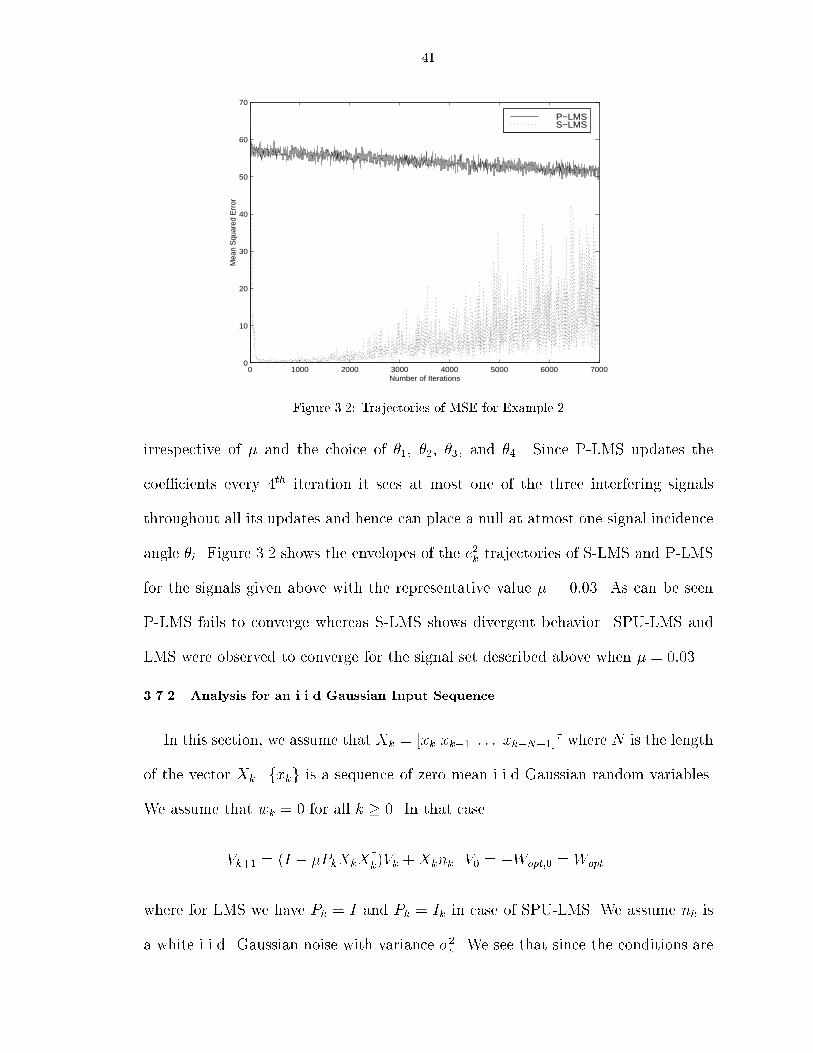
41

0 1000 2000 3000 4000 5000 6000 70000

10

20

30

40

50

60

70

Number of Iterations

Mea

n S

quar

ed E

rror

P−LMSS−LMS

Figure 3.2: Trajectories of MSE for Example 2irrespective of � and the choice of �1, �2, �3, and �4. Since P-LMS updates thecoe�cients every 4th iteration it sees at most one of the three interfering signalsthroughout all its updates and hence can place a null at atmost one signal incidenceangle �i. Figure 3.2 shows the envelopes of the e2k trajectories of S-LMS and P-LMSfor the signals given above with the representative value � = 0:03. As can be seenP-LMS fails to converge whereas S-LMS shows divergent behavior. SPU-LMS andLMS were observed to converge for the signal set described above when � = 0:03.3.7.2 Analysis for an i.i.d Gaussian Input SequenceIn this section, we assume that Xk = [xk xk�1 : : : xk�N+1]� where N is the lengthof the vector Xk. fxkg is a sequence of zero mean i.i.d Gaussian random variables.We assume that wk = 0 for all k � 0. In that caseVk+1 = (I � �PkXkXyk)Vk +Xknk V0 = �Wopt;0 = Woptwhere for LMS we have Pk = I and Pk = Ik in case of SPU-LMS. We assume nk isa white i.i.d. Gaussian noise with variance �2v . We see that since the conditions are

42satis�ed for theorem III.1 both LMS and SPU-LMS are exponentially stable. In factboth have the same � of decay. Therefore, conditions F1 and F2 are satis�ed.We rewrite Vk = J (0)k + J (1)k + J (2)k +H(2)k . Since, we have chosen �Fk = E[Fk] wehave E[PkXkXyk] = �2I in the case of LMS and 1P �2I in the case of SPU-LMS. By[55] and Lemmas 1 and 2 we can upperbound both J (2)k and H(2)k by exactly the sameconstants for LMS and SPU-LMS. From [55] and Lemmas 1 and 2 we have that thereexists some constant C <1 such that for all � 2 (0; �0], we havesupt�0 ���E[J (1)t (J (2)t +H(2)t )y]��� � CkX0kr(r+�)=��2r(v)�1=2supt�0 ���E[J (0)t H(2)t ]��� � C�r(v)kX0kr(r+�)=��1=2Therefore, for LMS we concentrate onJ (0)k+1 = (1� ��2)J (0)k +XknkJ (1)k+1 = (1� ��2)J (1)k + �(�2I �XkXyk)J (0)kand for SPU-LMS we concentrate onJ (0)k+1 = (1� �P �2)J (0)k + IkXknkJ (1)k+1 = (1� �P �2)J (1)k + �(�2P I � IkXkXyk)J (0)kSolving (see Appendix .5), we obtain for LMSlimk!1E[J (0)k (J (0)k )y] = �2v�(2� ��2)Ilimk!1E[J (0)k (J (1)k )y] = 0limk!1E[J (0)k (J (2)k )y] = 0limk!1E[J (1)k (J (1)k )y] = N�2�2v(2� ��2)2 I= N�2�2v4 I +O(�)I

43which yields limk!1E[VkV yk ] = �2v2�I + N�2�2v4 I +O(�)I and for SPU-LMS we obtainlimk!1E[J (0)k (J (0)k )y] = �2v�(2� �P �2)Ilimk!1E[J (0)k (J (1)k )y] = 0limk!1E[J (0)k (J (2)k )y] = 0limk!1E[J (1)k (J (1)k )y] = (N+1)P�1P �2�2v(2� �P �2)2 I= (N+1)P�1P �2�2v4 I +O(�)Iwhich yields limk!1E[VkV yk ] = �2v2�I + (N+1)P�1P �2�2v4 I +O(�)I. Therefore, we see thatSPU-LMS is marginally worse than LMS.3.7.3 Temporally Correlated Spatially Uncorrelated Array OutputIn this section we consider Xk given byXk = �Xk�1 +p1� �2Ukwhere Uk is a vector of circular Gaussian random variables with unit variance. Similarto section 3.7.2, we rewrite Vk = J (0)k + J (1)k + J (2)k + H(2)k . Since, we have chosen�Fk = E[Fk] we have E[PkXkXyk] = I in the case of LMS and 1P I in the case ofSPU-LMS. Again, conditions F1 and F2 are satis�ed because of Theorem III.1. By[55] and Lemmas 1 and 2 we can upperbound both J (2)k and H(2)k by exactly the sameconstants for LMS and SPU-LMS. From [55] and Lemmas 1 and 2 we have that thereexists some constant C <1 such that for all � 2 (0; �0], we havesupt�0 ���E[J (1)t (J (2)t +H(2)t )y]��� � CkX0kr(r+�)=��2r(v)�1=2supt�0 ���E[J (0)t H(2)t ]��� � C�r(v)kX0kr(r+�)=��1=2

44Therefore, for LMS we concentrate onJ (0)k+1 = (1� �)J (0)k +XknkJ (1)k+1 = (1� �)J (1)k + �(I �XkXyk)J (0)kand for SPU-LMS we concentrate onJ (0)k+1 = (1� �P )J (0)k + IkXknkJ (1)k+1 = (1� �P )J (1)k + �( 1P I � IkXkXyk)J (0)kSolving (see Appendix .6), we obtain for LMSlimk!1E[J (0)k (J (0)k )y] = �2v�(2� �)Ilimk!1E[J (0)k (J (1)k )y] = � �2�2vN2(1� �2)I +O(�)Ilimk!1E[J (0)k (J (2)k )y] = �2�2vN4(1� �2)I +O(�)Ilimk!1E[J (1)k (J (1)k )y] = (1 + �2)�2vN4(1� �2) I +O(�)Iwhich leads to limk!1E[VkV yk ] = �2v2�I + N�2v4 I +O(�)I and for SPU-LMS we obtainlimk!1E[J (0)k (J (0)k )y] = �2v�(2� �P )Ilimk!1E[J (0)k (J (1)k )y] = � �2�2vN2(1� �2)P I +O(�)Ilimk!1E[J (0)k (J (2)k )y] = �2�2vN4(1� �2)P I +O(�)Ilimk!1E[J (1)k (J (1)k )y] = �2v4 [NP 1 + �21� �2 + (N + 1)P � 1P ]I +O(�)Iwhich leads to limk!1E[VkV yk ] = �2v2�I + �24 [N + 1� 1P ]I +O(�)I. Again, SPU-LMSis marginally worse than LMS.3.8 Conclusion and Future WorkWe have proposed a new algorithm based on randomization of �lter coe�cientsubsets for partial updating of �lter coe�cients. The conditions on step-size for

45convergence-in-mean and mean-square were shown to be equivalent to those of stan-dard LMS. It was veri�ed by theory and by simulation that LMS and SPU-LMShave similar regions of convergence. We also have shown that the Stochastic PartialUpdate LMS algorithm has the same performance as the Periodic LMS algorithmfor stationary signals but, can have superior performance for some cyclo-stationaryand deterministic signals.The idea of random choice of subsets proposed in the chapter can be extended toinclude arbitrary subsets of size NP and not just subsets from a particular partition.No special advantage is immediately evident from this extension though.

CHAPTER IVCapacity: Isotropically Random Rician Fading4.1 IntroductionIn this chapter, we analyze a mobile wireless link with a line of sight component(specular component) and a di�use component (rayleigh component) both changingover time. We model the specular component as isotropically random independentof the rayleigh component. Traditionally, in a rician model the fading coe�cientsare modeled as Gaussian with non-zero mean. We depart from the traditional modelin the sense that we model the mean (specular component) as time-varying andstochastic. The specular component is modeled as an isotropic rank one matrixwith the specular component staying constant for T symbol durations and takingindependent values every T th instant. We establish that it is su�cient to optimizeover a smaller parameter set of size minfT;Mg of real valued magnitudes of thetransmitted signals instead of T �M complex valued symbols. The capacity achievingsignal matrix is shown to be the product of two independent matrices, a T � Tisotropically random unitary matrix and a T � M real nonnegative matrix. Thismodel is described in detail in section 4.2. In section 4.4, we derive a new lowerbound on capacity. The lower bound also holds for the case of a purely rayleighfading channel. In section 4.5 we show the utility of this bound by computing46

47capacity regions for both rayleigh and rician fading channels.4.2 Signal ModelThe fading channel is assumed to stay constant for T symbol periods and thentake on a completely independent realization, and so on. Let there be M transmitantennas and N receive antennas. We transmit a T �M signal matrix S and receivea T �N signal matrix X which are related as followsX =r �M SH +W (4.1)where the elements, wtn of W are independent circularly symmetric complex Gaus-sian random variables with mean 0 and variance 1 (CN (0; 1)).The only di�erence between the rayleigh model and the rician model consideredhere is in the statistics of the fading matrix H. In the case of the rayleigh model theelements hmn of H are modeled as independent CN (0; 1) random variables. Here forthe rician model, the matrix H is modeled asH = p1� rG+prNMv��ywhere G consists of independent CN (0; 1) random variables, v is a real randomvariable such that E[v2] = 1 and � and � are independent isotropically random unitmagnitude vectors of lengthM and N , respectively. G, � and � take on independentvalues every T th symbol period and remain unchanging in between. The parameterr ranges between zero and one, with the limits corresponding respectively to purelyrayleigh or specular propagation. Irrespective of the value of r, the average varianceof the components of H is equal to one, E[trfHHyg] =M �N .An M -dimensional unit vector � is isotropically random if its probability densityis invariant to pre-multiplication by an M �M deterministic unitary matrix, that

48is p(�) = p(�), 8 : y = IM . The isotropic density is p(�) = �(M)�M �(�y� � 1)([48]).The choice of p(v) the density of v is not clear. p(v) can be chosen to maximizethe entropy of R = v��y which is possibly the worst case scenario for the channelH. In that regard, we have the following proposition.Proposition IV.1. There is no distribution p(v) such that the elements of R =v��y have a joint Gaussian distribution, where � and � are isotropically randomunitary vectors, and v, �, and � are mutually independent.Proof: Proof is by contradiction. Consider the covariance of the elements, Rmn ofR. E[Rm1n1R�m2n2 ] = E[v2]E[�m1��m2 ]E[�n1��n2 ]= E[v2] 1M �m1m2�n1n2If elements of R were jointly Gaussian then they must be independent of each otherwhich contradicts the assumption that R is of rank one.From now on we will assume that v is identically equal to 1. In that case, theconditional probability density function is given byp(XjS) = E�E� "e�trf[IT+(1�r) �M SSy]�1(X�p�rNS��y)(X�p�rNS��y)yg�TN detN [IT + (1� r) �MSSy] #where E� denotes the expectation over the density of �.Irrespective of whether the fading is rayleigh or rician, we have p(yH) = p(H)for any M �M unitary matrix . In the rest of the section we will deal with Hsatisfying this property and refer to rayleigh and rician fading as special cases of thischannel. In that case, the condition probability density of the received signals hasthe following properties

491. For any T � T unitary matrix �p(�Xj�S) = p(XjS)2. For any M �M unitary matrix p(XjS) = p(XjS)We state some Lemmas without proof for lack of space. However, the reader isreferred to [48] for proofs of similar Lemmas.Lemma IV.1. If p(XjS) satis�es property 2 de�ned above then the transmitted sig-nal can be written as �V where � is a T � T unitary matrix and V is a T �M realnonnegative diagonal matrix.Proof: Let the input signal matrix S have the SVD �Vy then the channel canbe written as X =r �M�VyH +WNow, consider a new signal S1 formed by multiplying � and V and let X1 be thecorresponding received signal. ThenX1 =r �M�V H +WNote that X1 and X have exactly the same statistics since p(yH) = p(H). There-fore, one might as well send �V instead of �Vy.Corollary IV.1. If M > T then power should be transmitted only through T of theantennas.Proof: Note that the V in the signal transmitted, �V is T �M . It means thatV = [VT j0] where VT is T � T and 0 is T � (T �M). That meansX =r �M�VTHT +W

50where HT is the matrix of �rst T rows in H. That means power is transmitted viaonly through T transmit antennas instead of through all M .In the case of rayleigh Fading however Lemma IV.1 gives rise to a stronger result([48])Theorem IV.1. For any coherence interval T and any number of receiver antennas,the capacity obtained with M > T transmitter antennas is the same as the capacityobtained with M = T antennas.4.3 Properties of Capacity Achieving SignalsMarzetta and Hochwald [48] have established these results for the case of a purelyrayleigh fading channel but, the proofs were based only on the fact that the con-ditional probability density satis�es Properties 1 and 2 as stated in section 5.2.Therefore, these results are also applicable for the case of rician fading channel dis-cussed in this chapter. The capacity being calculated is under the power constraintE[trfSSyg] � TM .Lemma IV.2. : Suppose that S has a probability density p0(S) that generates somemutual information I0. Then, for any M �M unitary matrix and for any T � Tunitary matrix �, the \rotated" probability density, p1(S) = p0(�yS), also generatesI0.Proof: (For more details refer to the proof for Lemma 1 in [48].) The proofhinges on the fact that Jacobian determinant of any unitary transformation is one,p(�Xj�S) = p(XjS), p(XjSy) = p(XjS) and E[trfSSyg] is invariant to pre- andpost-multiplication of S by unitary matrices.Lemma IV.3. : For any transmitted signal probability density p0(S), there is a

51probability density p1(S) that generates at least as much mutual information and isunchanged by rearrangements of the rows and columns of S.Proof: (For more details refer to the proof for Lemma 2 in [48].) From Lemma IV.2it is evident any density obtained from the original density on S, p0(S) by pre- andpost-multiplying S by any arbitrary permutation matrices PTk, k = 1; : : : ; T ! (thereare T ! permutations of the rows) and PMl, l = 1; : : : ;M ! (there areM ! permutationsof the columns), generates the same mutual information. Since mutual informationis a concave functional of the input signal density a mixture input density, p1(S)formed by taking the average over all densities obtained by permuting S generatesa mutual information at least as large as that of the original density. Note that thenew mixture density satis�es the same power constraint as the original density sinceE[trfSSyg] is invariant to permutations of S.Corollary IV.2. : The following power constraints all yield the same channel ca-pacity.� Ejstmj2 = 1; m = 1; : : : ;M; t = 1; : : : ; T� 1M PMm=1Ejstmj2 = 1; t = 1; : : : ; T� 1T PTt=1 Ejstmj2 = 1; m = 1; : : : ;M� 1TM PTt=1PMm=1Ejstmj2 = 1Basically, the corollary tells us that tighter power constraints as shown abovedon't result in a decrease of capacity.Theorem IV.2. The signal matrix that achieves capacity can be written as S = �V ,where � is a T � T isotropically distributed unitary matrix, and V is an indepen-dent T � M real, nonnegative, diagonal matrix. Furthermore, we can choose the

52joint density of the diagonal elements of V to be unchanged by rearrangements of itsarguments.Proof: Proof is similar to the proof for Theorem 2 in [48].4.4 Capacity Upper and Lower BoundsFirst we will state the following result which has already been established in [48],and follows in a straightforward manner from [64].Theorem IV.3. The expression for capacity when only the receiver has completeknowledge about the channel isCH = T � E log det hIN + �MHyHiThe following upper bound on capacity is quite well known in the literature ([16],[48]).Proposition IV.2. An upper bound on capacity when neither the transmitter northe receiver has any knowledge about the channel is given byC � CH = T � E log det hIN + �MHyHi (4.2)The one thing that the literature lacks is a tractable lower bound on capacity. Inthis work we establish such a lower bound when no channel information is presentat either the transmitter or the receiver.Theorem IV.4. A lower bound on capacity when neither the transmitter nor thereceiver has any knowledge about the channel is given byC � TE hlog2 det�IN + �MHyH�i�NE hlog2 det�IT + �M SSy�i (4.3)� TE hlog2 det�IN + �MHyH�i�NM log2(1 + �M T ) (4.4)

53Proof: First note that the capacity C is given byC = maxp(S) [I(X;S) = H(X)�H(XjS)]by choosing a speci�c distribution on S, in this case CN (0; 1), we get a lower boundto C. Note that H(XjH) � H(X) so that we obtainC � H(XjH)�H(XjS) (4.5)Now, the expression on the right hand side in (4.5) can be rewritten as I(X;SjH)�I(X;HjS) which has a very intuitive meaning. I(X;SjH) is the mutual informationwhen H is known to the receiver and I(X;HjS) is the information contained in Xand S about H and therefore, I(X;HjS) can be viewed as the penalty for learningH in the course of decoding S from the reception of X.Since p(S) = 1�TM exp�trfSSyg (the elements of S are CN (0; 1) random variables)H(XjH) = TE hlog2 �(�e)N det�IN + �MHyH��iNow we turn to evaluating H(XjS). Note that since p(yH) = p(H) for all unitarymatrices , E[hm1n1h�m2n2 ] = �m1m2�n1n2 . Therefore given S, X has covariance givenby E[xt1n1x�t2n2 jS] = �n1n2 � "�t1t2 + �M MXm=1 st1ms�t2m#Since H(XjS) is bounded above by the entropy of a Gaussian with the same meanand covariance as XjS we haveHG(XjS) � NE hlog2 �(�e)T det�IT + �M SSy��iwhere the expectation is over the distribution of S which gives us (4.3). Note thatboth the expressions in the right hand side of (4.3) can be easily evaluated usingMonte Carlo simulations.

54However we can simplify the expression above further to obtain a looser lowerbound. We use the property that for any T � M matrix S, det(IT + SSy) =det(IM +SyS). This, along with the fact that log2 det(K) is convex cap and Jensen'sinequality, givesNE hlog2 det�IT + �M SSy�i � N log2 det�IM + �ME[SyS]� (4.6)= NM log2(1 + �M T ) (4.7)Therefore, we obtain (4.4).A simple improved lower bound in either (4.3) or (4.4) can be obtained by opti-mizing over the number of transmit and receive antennas used.From the new lower bound we can easily prove that as T !1 the normalized ca-pacity, Cn = C=T in bits per second per Hertz is given by Cn = E log det �IN + �MHyH�.This was conjectured by Marzetta and Hochwald in [48] and discussed in [16, p. 2632].4.5 Numerical ResultsFirst we show the utility of the lower bound by comparing it with the actualcapacity curve calculated in [48] for the case of a single transmit and receive antennasin a purely rayleigh fading environment for increasing T . We plot the upper bound,the lower bound derived in this work and the actual capacity in �gure 4.1. Theutility of this bound is clearly evident from how well the lower bound follows theactual capacity.In di�erent simulations, using the upper and lower bounds, we found that thecapacity variations as the channel moves from a purely rayleigh to a purely ricianchannel become more and more visible as we move to higher SNR regimes and largernumber of transmit and receive antennas. Examples of this behaviour are shown in�gures 4.2 and 4.3. Note that for the special case of M = N = 1 the capacity curves

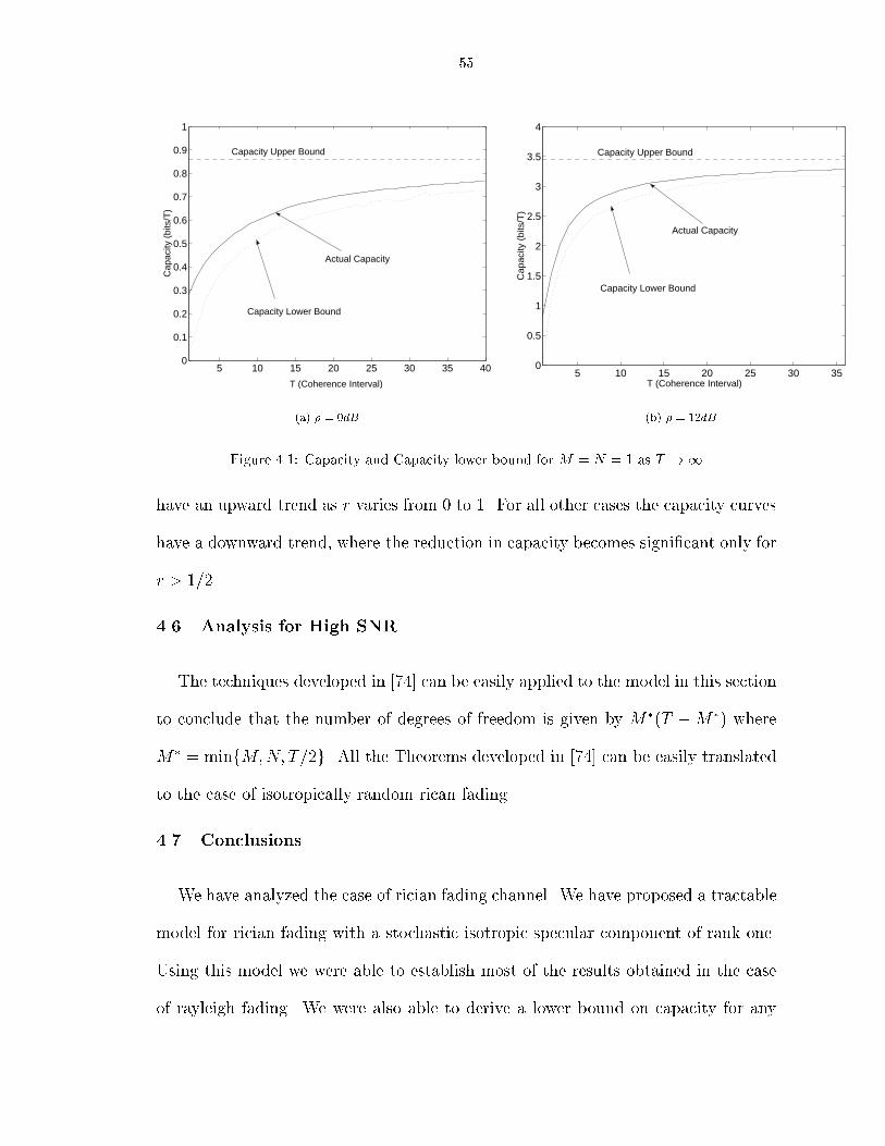
55

5 10 15 20 25 30 35 400

0.1

0.2

0.3

0.4

0.5

0.6

0.7

0.8

0.9

1

T (Coherence Interval)

Cap

acity

(bi

ts/T

)

Capacity Upper Bound

Capacity Lower Bound

Actual Capacity

(a) � = 0dB 5 10 15 20 25 30 350

0.5

1

1.5

2

2.5

3

3.5

4

T (Coherence Interval)

Cap

acity

(bi

ts/T

)

Capacity Upper Bound

Capacity Lower Bound

Actual Capacity

(b) � = 12dBFigure 4.1: Capacity and Capacity lower bound for M = N = 1 as T !1have an upward trend as r varies from 0 to 1. For all other cases the capacity curveshave a downward trend, where the reduction in capacity becomes signi�cant only forr > 1=2.4.6 Analysis for High SNRThe techniques developed in [74] can be easily applied to the model in this sectionto conclude that the number of degrees of freedom is given by M�(T �M�) whereM� = minfM;N; T=2g. All the Theorems developed in [74] can be easily translatedto the case of isotropically random rican fading.4.7 ConclusionsWe have analyzed the case of rician fading channel. We have proposed a tractablemodel for rician fading with a stochastic isotropic specular component of rank one.Using this model we were able to establish most of the results obtained in the caseof rayleigh fading. We were also able to derive a lower bound on capacity for any

56

0 0.1 0.2 0.3 0.4 0.5 0.6 0.7 0.8 0.9 10

1

2

3

4

5

6

7

8

9M = N = 2

r (fraction of power in Rician component)

Cap

acity

(bi

ts/T

)

Upper Bound, T = 4, 8, 16

Lower Bound, T = 16

Lower Bound, T = 8

Lower Bound, T = 4

(a) � = 0dB 0 0.1 0.2 0.3 0.4 0.5 0.6 0.7 0.8 0.9 10

1

2

3

4

5

6

7

8

9M = N = 2

r (fraction of power in Rician component)

Cap

acity

(bi

ts/T

)

Upper Bound, T = 4, 8, 16

Lower Bound, T = 16

Lower Bound, T = 8

Lower Bound, T = 4

(b) � = 15dBFigure 4.2: Capacity upper and lower bounds as the channel moves from purely rayleigh to purelyrician fading

0 0.2 0.4 0.6 0.8 10

2

4

6

8

10

12

14

16

18

20N = 4

r (fraction of power in Rician component)

Cap

acity

(bi

ts/T

)

T = 2, M = 1 T = 4, M = 2 T = 8, M = 4

(a) � = 0dB 0 0.2 0.4 0.6 0.8 10

2

4

6

8

10

12

14

16

18

20N = 4

r (fraction of power in Rician component)

Cap

acity

(bi

ts/T

)

T = 2, M = 1 T = 4, M = 2 T = 8, M = 4

(b) � = 15dBFigure 4.3: Capacity upper and lower bounds as the channel moves from purely rayleigh to purelyrician fading

57number of transmit and receive antennas. This lower bound is also applicable tothe case of rayleigh fading. For single transmit and receive antennas, the ricianchannel gives superior performance with respect to the rayleigh channel. For multipleantenna channels, rician fading tends to degrade the performance. Our numericalresults indicate that the rayleigh model is surprisingly robust, however: under ourrician model, up to half of the received energy can arrive via the specular componentwithout signi�cant reduction in capacity compared with the purely rayleigh case.

CHAPTER VMin-Capacity: Rician Fading, Unknown Static SpecularComponent5.1 IntroductionIn the previous chapter we considered a non-conventional model for the case ofrician fading where the fading channel consists of a rayleigh component, modeled asin [48] and an independent rank-one isotropically distributed specular component.The fading channel was assumed to remain constant over a block of T consecutivesymbol periods but take a completely independent realization over each block. Wederived similar results on optimal capacity achieving signal structures as in [48].We also established a lower bound to capacity that can be easily extended to themodel considered in this chapter. The model described in the previous chapter isapplicable to a mobile-wireless link where both the direct line of sight component(specular component) and the di�use component (rayleigh component) change withtime.In this chapter, we consider a quasi-static rician model where the specular compo-nent is non-changing while the rayleigh component is varying over time. This modelis similar to the traditional model where the specular component is deterministicand persists over time. The model is applicable to the case where the transmitterand receiver are �xed in space or are in motion but su�ciently far apart so that the58

59specular component is practically constant while the di�use multipath componentchanges rapidly. If the specular component were known to both the transmitter andthe receiver then the signaling scheme as well as the capacity would depend on thespeci�c realization of the specular component. We however deal with the case whenthe transmitter has no knowledge about the specular component. In this scenariothe transmitter can either maximize the worst case rate over the ensemble of valuesthat the specular component can take or maximize the average rate by establishinga prior distribution on the ensemble. We address both approaches in this chapter.Similarly to [19] the specular component is an outer product of two vectors ofunit magnitude that are non-changing and unknown to the transmitter but knownto the receiver. The di�erence between our approach and that of [19] is that in [19]the authors consider the channel to be known completely to the receiver. We assumethat the receiver's extent of knowledge about the channel is limited to the specularcomponent. That is, the receiver has no knowledge about the rayleigh component ofthe model. Considering the absence of knowledge at the transmitter it is importantto design a signal scheme that guarantees the largest overall rate for communicationirrespective of the value of the specular component. This is formulated as the problemof determining the worst case capacity in section 5.2. In section 5.5 we consider theaverage capacity instead of worst case capacity and show that both formulationsimply the same optimal signal structure and the same maximum possible rate.5.2 Signal Model and Problem FormulationLet there be M transmit antennas and N receive antennas. We assume that thefading coe�cients remain constant over a block of T consecutive symbol periods butare independent from block to block. Keeping that in mind, we model the channel

60as carrying a T �M signal matrix S over a M �N MIMO channel H, producing Xat the receiver according to the model:X =r �M SH +W (5.1)where the elements, wtn of W are independent circular complex Gaussian randomvariables with mean 0 and variance 1 (CN (0; 1)).The MIMO rician model for the matrix H is H = p1� rG +prNM��y whereG consists of independent CN (0; 1) random variables and � and � are deterministicvectors of lengthM and N , respectively, such that �y� = 1 and �y� = 1. We assume� and � are known to the receiver. Since the receiver is free to apply a co-ordinatetransformation by post multiplyingX by a unitary matrix, without loss of generalitywe can take � to be identically equal to [1 0 : : : 0]T . We will sometimes write H asH� to highlight the dependence of H on �. G remains constant for T symbol periodsand takes on a completely independent realization every T th symbol period.The problem we are investigating is to �nd the distribution pm(S) that attains themaximum in the following maximization de�ning the worst case channel capacityCm = maxp(S) Im(X;S) = maxp(S) inf�2A I�(X;S)and also to �nd the maximum value, Cm.I�(X;S) = Z p(S)p(XjS; ��y) log p(XjS; ��y)R p(S)p(XjS; ��y) dS dSdXis the mutual information between X and S when the specular component is givenby ��y and A def= f� : � 2 Cl M and �y� = 1g. Since A is compact the \inf" in theproblem can be replaced by \min". For convenience we will refer to Im(X;S) as themin-mutual information and Cm as min-capacity.The min-capacity de�ned above is just the capacity of a compound channel. Formore information on the concept of compound channels and worst case capacity

61please refer to [7, chapter 5, pp. 172-178]. It is shown that [7, Prob. 13, p. 183]min-capacity doesn't depend on the receiver's knowledge of the channel. Hence, it isnot necessary for us to assume that the specular component is known to the receiver.However, we do so because it facilitates easier description of min-capacity in termsof the conditional probability distribution p(XjS).5.3 Capacity Upper and Lower BoundsTheorem V.1. Min-capacity, CmH when the channel matrix H is known to the re-ceiver but not to the transmitter is given byCmH = TE log det hIN + �MHye1He1i (5.2)where e1 = [1 0 : : : 0]T is a unit vector inCl M . Note that e1 in (5.2) can be replacedby any � 2 A without changing the answer. Proof: First we note that for T > 1,given H the channel is memoryless and hence the columns of the input signal matrixS are independent of each other. That means the mutual information I�(X;S) =PTi=1 I�(Xi;Si) where Xi and Si denote the ith row of X and S, respectively. Themaximization over each term can be done separately and it is easily seen that eachterm will be maximized individually for the same density on Si. That is p(Si) =p(Sj) for i 6= j and maxp(S) I�(X;S) = T maxp(S1) I�(X1;S1). Therefore, WLOG weassume T = 1.Given H the channel is an AWGN channel therefore, capacity is attained byGaussian signal vectors. Let �S be the input signal covariance. Since the transmitterdoesn't know �, �S can not depend on � and the min-capacity is given bymax�S:trf�Sg�M F(�S) = max�S:trf�Sg�Mmin�2A E log det hIN + �MHy��SH�i (5.3)where F(�S) is implicitly de�ned in an obvious manner. First note that F(�S) in(5.3) is a concave function of �S (This follows from the fact that log detK is a concave

62function of K). Also, F(y�S) = F(�S) for any M �M : y = IM sincey� 2 A for any � 2 A and G has i.i.d. zero mean complex Gaussian entries. LetQyDQ be the SVD of �S then we have F(D) = F(QyDQ) = F(�S). Therefore, wecan choose �S to be diagonal. Moreover, F(P yk�SPk) = F(�S) for any permutationmatrix Pk, k = 1; : : : ;M !. Therefore, if we choose �0S = 1M !PM !k=1 P yk�SPk then byconcavity and Jensen's inequality we haveF(�0S) � M !Xk=1 F(P yk�SPk) = F(�S)Therefore, we conclude that the maximizing input signal covariance �S is a multipleof the identity matrix. It is quite obvious to see that to maximize the expressionin (5.3) we need to choose trf�Sg = M or �S = IM and since E log det[IN +�MHy�1H�1 ] = E log det[IN + �MHy�2H�2 ] for any �1; �2 2 A, (5.2) easily follows.By the data processing theorem additional information at the receiver doesn'tdecrease capacity. Therefore:Proposition V.1. An upper bound on the channel min-capacity when neither thetransmitter nor the receiver has any knowledge about the channel is given byCm � T � E log det hIN + �MHye1He1i (5.4)Now, we establish a lower bound.Proposition V.2. A lower bound on min-capacity when the transmitter has noknowledge about H and the receiver has no knowledge about G is given byCm � CmH �NE hlog2 det�IT + (1� r) �M SSy�i (5.5)� CmH �NM log2(1 + (1� r) �M T ) (5.6)Proof: Proof is similar to that of Theorem IV.4 and won't be repeated here.Combining (5.4) and (4.4) gives us the following

63Corollary V.1. The normalized min-capacity, Cmn = Cm=T in bits per second perHertz as T !1 is given byCmn = E log det hIN + �MHye1He1iNote that this is same as the capacity when the receiver knows H, so that asT !1 perfect channel estimation can be performed.5.4 Properties of Capacity Achieving SignalsIn this section, we derive the optimum signal structure for achieving min-capacity.The optimization is being done under the power constraint E[trfSSyg] � TM .Lemma V.1. Im(X;S) as a functional of p(S) is concave in p(S).Proof: First we note that I�(X;S) is a concave functional of p(S) for every � 2 A.Let Im(X;S)p(S) denote Im(X;S) evaluated using p(S) as the signal density. Then,Im(X;S)�p1(S)+(1��)p2(S) = min�2A I�(X;S)�p1(S)+(1��)p2(S)� min�2A [�I�(X;S)p1(S) + (1� �)I�(X;S)p2(S)]� �min�2A I�(X;S)p1(S) + (1� �)min�2A I�(X;S)p2(S)= �Im(X;S)p1(S) + (1� �)Im(X;S)p2(S)Lemma V.2. For any T � T unitary matrix � and any M �M unitary matrix ,if p(S) generates Im(X;S) then so does p(�Sy).Proof: 1) Note that p(�Xj�S) = p(XjS), therefore I�(X; �S) = I�(X;S) forany T � T unitary matrix � and all � 2 A.2) We have, � 2 A for any � 2 A and any M �M unitary matrix . Therefore,if Im(X;S) achieves its minimum value at �0 2 A then Im(X;Sy) achieves its

64minimum value at �0 because I�(X;S) = I�(X;Sy) for � 2 A and anM�Munitary matrix.Combining 1) and 2) we get the lemma.Lemma V.3. The min-capacity achieving signal distribution, p(S) is unchanged byany pre- and post- multiplication of S by unitary matrices of appropriate dimensions.Proof: We will show that for any signal density p0(S) generating min-mutualinformation Im0 there exists a density p1(S) generating Im1 � Im0 such that p1(S) isinvariant to pre- and post- multiplication of S by unitary matrices of appropriatedimensions. By Lemma V.2, for any pair of permutation matrices, � (T � T ) and (M �M) p0(�Sy) generates the same min-mutual information as p(S). De�neuT (�) to be the isotropically random unitary density function of a T � T unitarymatrix �. Similarly de�ne uM(). Let p1(S) be a mixture density given as followsp1(S) = Z Z p0(�Sy)u(�)u() d�dIt is easy to see that p1(S) is invariant to any pre- and post- multiplication of S byunitary matrices and if Im1 is the min-mutual information generated by p1(S) thenfrom Jensen's inequality and concavity of Im(X;S) we have Im1 � Im0 .Corollary V.2. pm(S), the optimal min-capacity achieving signal density lies inP = [I>0PI where PI = fp(S) : I�(X;S) = I 8� 2 Ag (5.7)Proof: Follows immediately from Lemma V.3 because any signal density that isinvariant to pre- and post- multiplication of S by unitary matrices generates thesame mutual information I�(X;S) irrespective of the value of �.

65Corollary V.3. The min-capacity achieving signal distribution p(S) is unchangedby rearrangements of elements in S.Corollary V.4. : The following power constraints all yield the same channel min-capacity.� Ejstmj2 = 1; m = 1; : : : ;M; t = 1; : : : ; T� 1M PMm=1Ejstmj2 = 1; t = 1; : : : ; T� 1T PTt=1 Ejstmj2 = 1; m = 1; : : : ;M� 1TM PTt=1PMm=1Ejstmj2 = 1Theorem V.2. The signal matrix that achieves min-capacity can be written as S =�Vy, where � and are T � T and M � M isotropically distributed matricesindependent of each other, and V is a T � M real, nonnegative, diagonal matrix,independent of both � and .Proof: From the singular value decomposition (SVD) we can write S = �Vy,where � is a T � T unitary matrix, V is a T �M nonnegative real diagonal matrix,and is an M �M unitary matrix. In general, �, V and are jointly distributed.Suppose S has probability density p0(S) that generates min-mutual information Im0 .Let �1 and �2 be isotropically distributed unitary matrices of size T �T andM�Mindependent of S and of each other. De�ne a new signal S1 = �1S�y2, generatingmin-mutual information Im1 . Now conditioned on �1 and �2, the min-mutual informationgenerated by S1 equals Im0 . From the concavity of the min-mutual information as afunctional of p(S), and Jensen's inequality we conclude that Im1 � Im0 .Since �1 and �2 are isotropically distributed �1� and �2 are also isotropicallydistributed when conditioned on � and respectively. This means that both �1�

66and �2 are isotropically distributed making them independent of �, V and .Therefore, S1 is equal to the product of three independent matrices, a T �T unitarymatrix �, a T �M real nonnegative matrix V and an M �M unitary matrix .Now, we will show that the density p(V ) on V is unchanged by rearrangements ofdiagonal entries of V . There are minfM !; T !g ways of arranging the diagonal entriesof V . This can be accomplished by pre- and post-multiplying V by appropriatepermutation matrices, PTk and PMk, k = 1; : : : ;minfM !; T !g. The permutationdoesn't change the min-mutual information because �PTk and PMk have the samedensity functions as � and . By choosing an equally weighted mixture densityfor V , involving all minfM !; T !g arrangements we obtain a higher value of min-mutual information because of concavity and Jensen's inequality. This new densityis invariant to the rearrangements of the diagonal elements of V .5.5 Average Capacity CriterionIn this case we maximize IE(X;S) = E�[I�(X;S)], where I� is as de�ned earlierand E� denotes expectation over � 2 A under the assumption that all � are equallylikely. That is, under the assumption that � is unchanging over time, isotropicallyrandom and known to the receiver. Please note that this di�ers from the modelconsidered in [29] where the authors consider the case of a piecewise constant, timevarying, i.i.d. specular component.Therefore, the problem can be stated as �nding pE(S) the probability densityfunction on the input signal S that achieves the following maximizationCE = maxp(S) E�[I�(X;S)] (5.8)and also to �nd the value CE. We will refer to IE(X;S) as avg-mutual informationand CE as avg-capacity.

67We will show that the signal density pm(S) that attains Cm also attains CE. Forthat we need to establish the following Lemmas.Lemma V.4. IE(X;S) is a concave functional of the signal density p(S)Proof: First we note that I�(X;S) is a concave functional of p(S) for every � 2 A.Then,IE(X;S)�p1(S)+(1��)p2(S) = E�[I�(X;S)�p1(S)+(1��)p2(S)]� E�[�I�(X;S)p1(S) + (1� �)I�(X;S)p2(S)]= �E�[I�(X;S)p1(S)] + (1� �)E�[I�(X;S)p2(S)]= �IE(X;S)p1(S) + (1� �)IE(X;S)p2(S)Lemma V.5. For any T � T unitary matrix � and any M �M unitary matrix ,if p(S) generates IE(X;S) then so does p(�Sy).Proof: We want to show if p(S) generates IE(X;S) then so does p(�Sy). Nowsince the density function of �, p(�) = �(M)�M �(�y�� 1) we haveIE(X;S) = �M�(M) Z I�(X;S) d�Note that I�(X; �S) = I�(X;S) and I�(X;Sy) = I�(X;S) ) Iy�(X;S) =I�(X;Sy). Therefore,I 0E(X;S) = �M�(M) Z I�(X; �Sy) d�= �M�(M) Z I�(X;Sy) d�= �M�(M) Z Iy�(X;S) d�= �M�(M) Z I!(X;S) d!= IE(X;S)

68where the last two equalities follow from the transformation ! = y� and the factthe Jacobian of the transformation is equal to 1.Lemma V.6. The avg-capacity achieving signal distribution, p(S) is unchanged byany pre- and post- multiplication of S by unitary matrices of appropriate dimensions.Corollary V.5. pm(S), the optimal avg-capacity achieving signal density lies in P =[I>0PI where PI is as de�ned in (5.7).Based on the last corollary we conclude that for a given p(S) in P we haveIm(X;S) = min�2A I�(X;S) = E�[I�(X;S)] = IE(X;S). Therefore, the maximiz-ing densities for CE and Cm are the same and also CE = Cm. Therefore, designingthe signal constellation with the objective of maximizing the worst case performanceis not more pessimistic than maximizing the average performance.5.6 ConclusionsWe have proposed another tractable model for rician fading channel di�erent fromthe one in chapter IV but, along the lines of [19]. We were able to analyze this channeland derive some interesting results on optimal signal structure. We were also able toshow that the optimization e�ort is over a much smaller set of parameters than theset originally started with. We were also able to derive a lower bound that is veryuseful because capacity computations in general are not tractable.Finally, we were able to show that the approach of maximizing the worst casescenario is not overly pessimistic in the sense that the signal density maximizing theworst case performance also maximizes the average performance and the capacityvalue in both formulations turns out to be the same.

CHAPTER VICapacity: Rician Fading, Known Static Specular Component6.1 IntroductionIn the previous chapters we had not considered the case of the standard ricianmodel where the specular component is deterministic and known to both the trans-mitter and the receiver. In chapter IV, we considered a model where the specularcomponent is rank-one and has an isotropic distribution. In chapter V, we considereda model where the specular component is deterministic and static but unknown tothe transmitter. Both these models led to a tractable analysis of the capacity of arician fading model. Also, the specular component considered in both the chapterswas of rank one.In this chapter, we analyze the standard rician fading model for capacity. Through-out the chapter, we assume that the specular component is deterministic and is knownto both the transmitter and the receiver. The specular component in this chapteris of general rank except in section 6.2 where it is restricted to be of rank one. Therayleigh component is never known to the transmitter. There are some cases weconsider where the receiver has complete knowledge of the channel. In such cases,the receiver has knowledge about the rayleigh as well as the specular componentwhereas the transmitter has knowledge only about the specular component. The ca-69

70pacity when the receiver has complete knowledge about the channel will be referredto as coherent capacity and the capacity when the receiver has no knowledge aboutthe rayleigh component will be referred to as non-coherent capacity. This chapteris organized as follows. In section 6.2 we deal with the special case of a rank-onespecular component with the characterization of coherent capacity in section 6.2.1.The general case of no restrictions on the rank of the specular component is dealtwith in section 6.3. The coherent capacity for this case is considered in section 6.3.1,the non-coherent capacity for low SNR in section 6.3.3 and the non-coherent capacityfor high SNR in section 6.3.4. Finally, in section 6.4 we consider the performance ofa rician channel in terms of capacity when pilot symbol based training is used in thecommunication system.6.2 Rank-one Specular ComponentThe model for the rician fading channel being considered here isX =r �M SH +W (6.1)whereX is the T�N matrix of received signals,H is theM�N matrix of propagationcoe�cients, S is the T�M matrix of transmitted signals andW is the T�N matrix ofadditive noise components and � is the expected signal to noise ratio at the receivers.For a deterministic rank one rician channel H is de�ned as H = p1� rG +prNMHm where G consists of independent CN (0; 1) random variables, Hm isM�Ndeterministic matrix of rank one such that trfHymHmg = 1 and r is a number lyingbetween 0 and 1 known to both the transmitter and the receiver. ThereforeHm = ��ywhere � is a length M vector and � is a length N vector such that �y� = �y� = 1.It is assumed that Hm is known to both the receiver and the transmitter. Therefore,

71WLOG we can assume thatHm = 2666666664

10...03777777775 [1 0 : : : 0] (6.2)

where the column and row vectors are of appropriate lengths.In this case, the conditional probability density function is given by,p(XjS) = e�trf[IT+(1�r)(�=M)SSy]�1(X�prNMSHm)(X�prNMSHm)yg�TN detN [IT + (1� r)(�=M)SSy]The conditional probability density enjoys the following properties1. For any T � T unitary matrix �p(�Xj�S) = p(XjS)2. For any (M � 1)� (M � 1) unitary matrix p(XjS) = p(XjS)where = 264 1 00y 375 (6.3)6.2.1 Coherent CapacityThe mutual information expression under the known H case has already beenderived in [21]. For known H the capacity achieving signal S is Gaussian independentfrom time instant to time instant. For this signal the expression isI(X;SjH) = T � E log det hIN + �MHy�Hi

72where � = E[S�t S�t ] for t = 1; : : : ; T where St is the tth row of the T �M matrix S.S�t denotes the transpose of St and S�t def= (S�t )y.Theorem VI.1. The capacity achieving signal covariance matrix is of the form� = 264 M � (M � 1)d LLy D 375where d is a positive real number such that 0 � d � M=(M �1) and D is the productof d and the identity matrix of dimension (M � 1)� (M � 1) and L is the productof a complex number, l (jlj � q( MM�1 � d)d) and an all ones row vector of lengthM � 1.Proof: This proof is a modi�cation of the proof in [64]. Using the property thatyH has the same distribution as H where is of the form given in 6.3 we concludethat T � E log det hIN + �MHy�Hi = T � E log det hIN + �MHy�yHiIf � is written as � = 264 c AAy B 375where c is a positive number such that c � AyB�1A (to ensure positive semi-de�niteness of the covariance matrix �), A is a column vector of length M � 1and B is a positive de�nite matrix of size (M � 1)� (M � 1). Then�y = 264 c A y Ay B y 375Since B = UDU y where D is a diagonal matrix and U is a unitary matrix of size(M � 1)� (M � 1), choosing = �U where � is a permutation matrix, we obtain

73that T � E log det hIN + �MHy�Hi = T � E log det hIN + �MHy��Hiwhere �� = 264 c AU y�y�UAy �D�y 375Since log det is a concave (convex cap) function we haveT � E log det hIN + �MHy �� Hi � T � 1(M � 1)!X� E log det hIN + �MHy��Hi= I(X;S)where �� = 1(M�1)!P� �� and the summation is over all possible permutation ma-trices which are (M � 1)! in number. Therefore, the capacity achieving � is given by1(M�1)!P� �� and is of the form � = 264 c LLy D 375Now, the capacity achieving signal matrix has to satisfy trf�g = M because iftrf�g < M then we can always multiply � by a constant greater than 1 which canonly increase the mutual information. Therefore, c = M � (M � 1)d. And sincec � LyD�1L this implies M � (M � 1)d � (M�1)jlj2d and we obtain the desired signalcovariance structure.The problem is to choose l and d to maximize I(X;S). This problem has ananalytical solution for the special cases of 1) r = 0 for which d = 1 and l = 0 and2) r = 1 for which d = l = 0. The optimization problem can be solved by usingthe method of steepest descent (See Appendix .7). Results for � = 100; 10; 1; 0:1 areshown in Figure 6.1. The optimum values of l for di�erent values of � turned out tobe zero. As can be seen from the plot the optimum value of d stays close to 1 for high

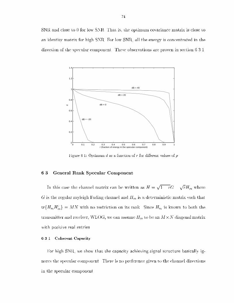
74SNR and close to 0 for low SNR. That is, the optimum covariance matrix is close toan identity matrix for high SNR. For low SNR, all the energy is concentrated in thedirection of the specular component. These observations are proven in section 6.3.1.

0 0.1 0.2 0.3 0.4 0.5 0.6 0.7 0.8 0.9 10

0.2

0.4

0.6

0.8

1

1.2

1.4

r (fraction of energy in the specular component)

d

dB = −20

dB = 0

dB = 20

dB = 40

Figure 6.1: Optimum d as a function of r for di�erent values of �6.3 General Rank Specular ComponentIn this case the channel matrix can be written as H = p1� rG +prHm whereG is the regular rayleigh Fading channel and Hm is a deterministic matrix such thattrfHmHymg = MN with no restriction on its rank. Since Hm is known to both thetransmitter and receiver, WLOG, we can assumeHm to be anM�N diagonal matrixwith positive real entries.6.3.1 Coherent CapacityFor high SNR, we show that the capacity achieving signal structure basically ig-nores the specular component. There is no preference given to the channel directionsin the specular component.

75Proposition VI.1. For high SNR, capacity, CH in the known H case is attained bya diagonal signal covariance matrix when M � N andCH � T � E log det[ �MHyH]Proof: The expression for capacity, CH isCH = T � E log det[IN + �MHy�H]Consider the following expression for a speci�c realization of the matrix H with SVDgiven by H = ��y thenlog det[IN + �MHy�H] = log det[IN + �M�y�y���]Let �y�� = D. Thenlog det[IN + �M�yD�] = log det[IM + �MD��y]The term above is maximized by choosing D to be diagonal ([10, page 255]). LetD = diagfd1; d2; : : : ; dMg and �i be the eigenvalues of ��y and EA[�] denote theexpectation conditioned on the event A, then for large �E log det[IM + �MD��y] = MXi=1 E�i<1=p� log[1 + �M di�i]| {z }=K +MXi=1 E�i�1=p� log[1 + �M di�i]| {z }=L= log �M + MXi=1 log(di) + MXi=1 E�i>1=p�[log(�i)] +O(log(p�)=p�)since K � log[1 +p�] MXi=1 P (�i < 1=p�) = O(log(p�)=p�)

76and L = log �M + MXi=1 log(di) + MXi=1 E�i>1=p�[log(�i)] +O(1=p�)On account of log being a convex cap function the �rst term in the expression onthe last line above is maximized by choosing di = d for i = 1; : : : ;M such thatM � d =M .For low SNR, we show that the rician fading channel essentially behaves like anAWGN channel in the sense that the rayleigh fading component has no e�ect on thestructure of the optimum covariance structure.Proposition VI.2. For low SNR, capacity, CH when H is known to the receiver isattained by the same signal covariance matrix that attains capacity when H = Hmor when r = 0, irrespective of the value of M and N andCH � �[r�max(HmHym) + (1� r)N ]Proof: We haveCH = T � E log det[IN + �MHy�H]= T � EkHk�1=� log det[IN + �MHy�H] + EkHk<1=� log det[IN + �MHy�H]= Etrf �MHy�Hg+O(�2�2 )This follows from the fact that P (kHk � 1=� ) < O(e� 1� =TM) and log det[IN +�MHy�H] = tr[ �MHy�H] +O(�2�2 ) for kHk < 1=� . Since is arbitraryE log det[IN + �MHy�H] = Etr[ �MHy�H] +O(�2)Now Etr[Hy�H] = trf(1� r)E[Gy�G] + rHym�Hm]g= trf(1� r)�E[GGy] + r�HmHymg

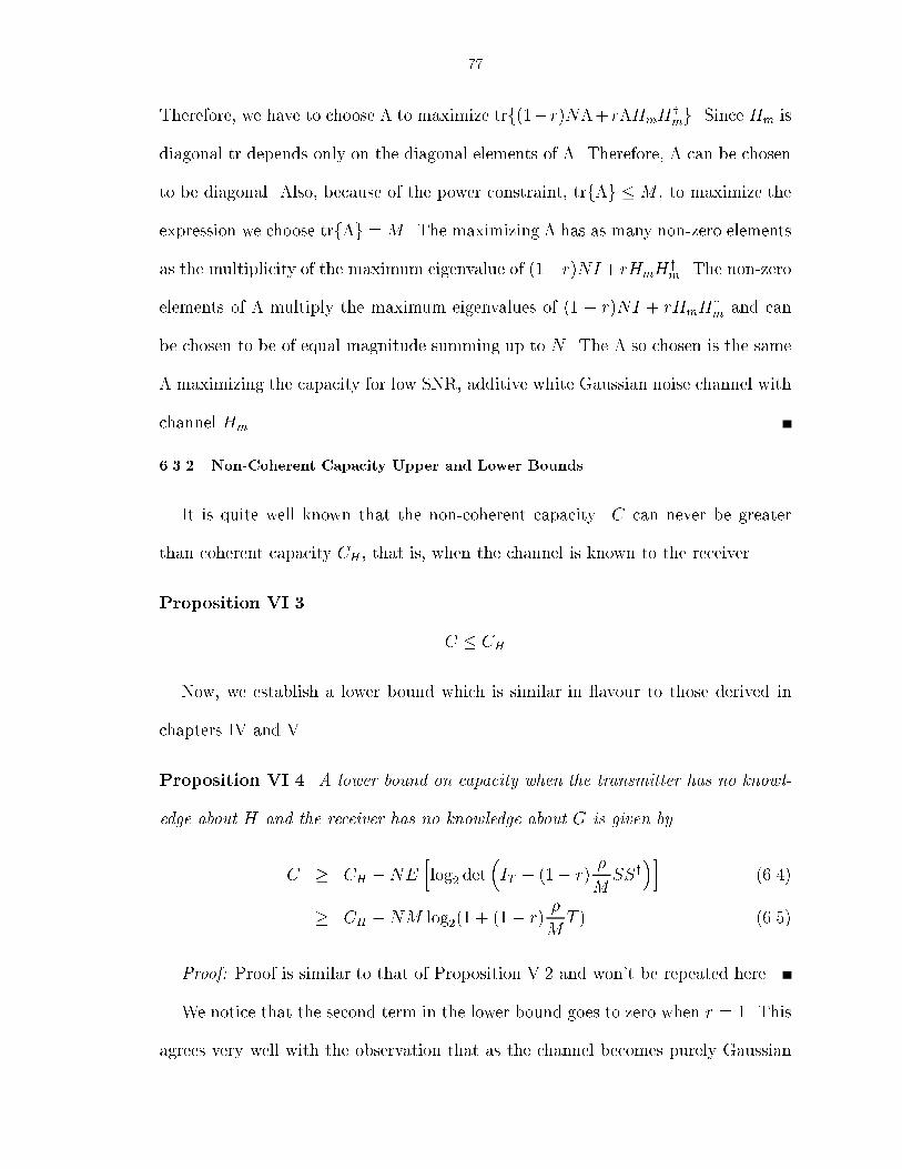
77Therefore, we have to choose � to maximize trf(1� r)N�+ r�HmHymg. Since Hm isdiagonal tr depends only on the diagonal elements of �. Therefore, � can be chosento be diagonal. Also, because of the power constraint, trf�g �M , to maximize theexpression we choose trf�g =M . The maximizing � has as many non-zero elementsas the multiplicity of the maximum eigenvalue of (1�r)NI+rHmHym. The non-zeroelements of � multiply the maximum eigenvalues of (1 � r)NI + rHmHym and canbe chosen to be of equal magnitude summing up to N . The � so chosen is the same� maximizing the capacity for low SNR, additive white Gaussian noise channel withchannel Hm.6.3.2 Non-Coherent Capacity Upper and Lower BoundsIt is quite well known that the non-coherent capacity. C can never be greaterthan coherent capacity CH , that is, when the channel is known to the receiver.Proposition VI.3. C � CHNow, we establish a lower bound which is similar in avour to those derived inchapters IV and V.Proposition VI.4. A lower bound on capacity when the transmitter has no knowl-edge about H and the receiver has no knowledge about G is given byC � CH �NE hlog2 det�IT + (1� r) �M SSy�i (6.4)� CH �NM log2(1 + (1� r) �M T ) (6.5)Proof: Proof is similar to that of Proposition V.2 and won't be repeated here.We notice that the second term in the lower bound goes to zero when r = 1. Thisagrees very well with the observation that as the channel becomes purely Gaussian

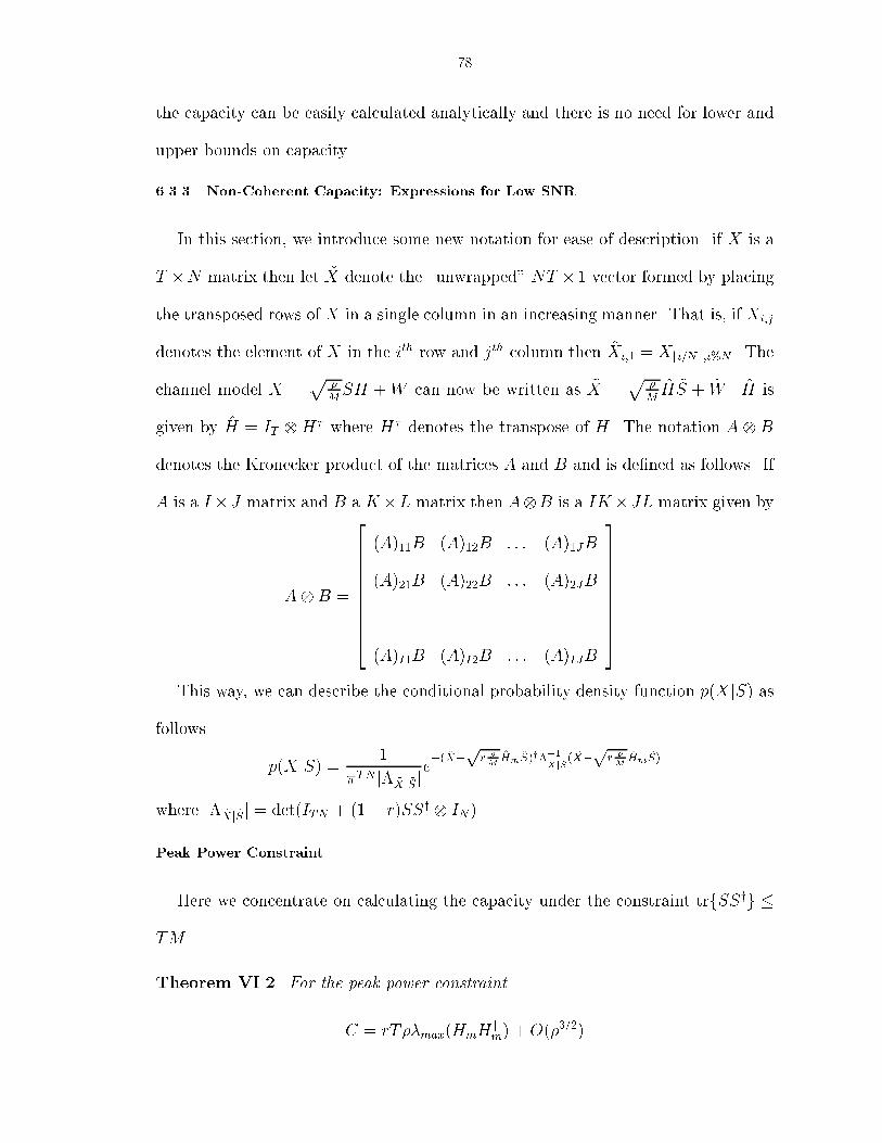
78the capacity can be easily calculated analytically and there is no need for lower andupper bounds on capacity.6.3.3 Non-Coherent Capacity: Expressions for Low SNRIn this section, we introduce some new notation for ease of description. if X is aT �N matrix then let ~X denote the \unwrapped" NT � 1 vector formed by placingthe transposed rows of X in a single column in an increasing manner. That is, if Xi;jdenotes the element of X in the ith row and jth column then ~Xi;1 = Xbi=Nc;i%N . Thechannel model X = p �MSH +W can now be written as ~X = p �M H ~S + ~W . H isgiven by H = IT H� where H� denotes the transpose of H. The notation A Bdenotes the Kronecker product of the matrices A and B and is de�ned as follows. IfA is a I�J matrix and B a K�L matrix then AB is a IK�JL matrix given byAB = 2666666664

(A)11B (A)12B : : : (A)1JB(A)21B (A)22B : : : (A)2JB... ... . . . ...(A)I1B (A)I2B : : : (A)IJB3777777775This way, we can describe the conditional probability density function p(XjS) asfollows p(XjS) = 1�TN j� ~Xj ~Sje�( ~X�pr �M Hm ~S)y��1~Xj ~S( ~X�pr �M Hm ~S)where j� ~Xj ~Sj = det(ITN + (1� r)SSy IN ).Peak Power ConstraintHere we concentrate on calculating the capacity under the constraint trfSSyg �TM .Theorem VI.2. For the peak power constraintC = rT��max(HmHym) +O(�3=2)

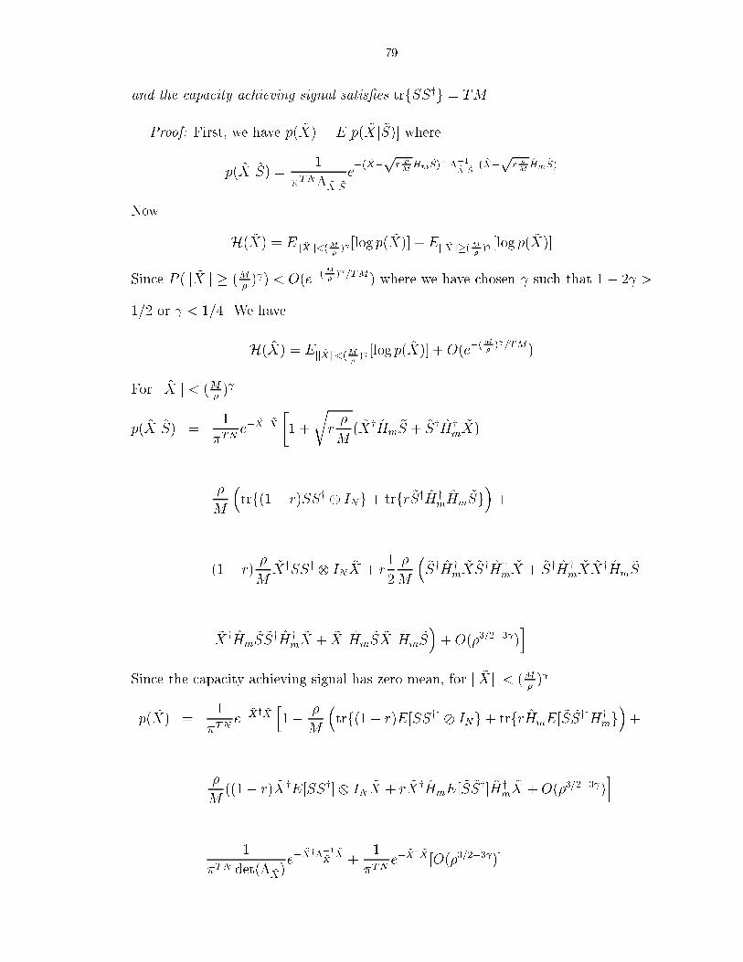
79and the capacity achieving signal satis�es trfSSyg = TM .Proof: First, we have p( ~X) = E[p( ~Xj ~S)] wherep( ~Xj ~S) = 1�TN� ~Xj ~S e�( ~X�pr �M Hm ~S)y ��1~Xj ~S ( ~X�pr �M Hm ~S)Now H( ~X) = Ek ~Xk<(M� ) [log p( ~X)] + Ek ~Xk�(M� ) [log p( ~X)]Since P (k ~Xk � (M� ) ) < O(e�(M� ) =TM) where we have chosen such that 1� 2 >1=2 or < 1=4. We haveH( ~X) = Ek ~Xk<(M� ) [log p( ~X)] +O(e�(M� ) =TM)For k ~Xk < (M� ) p( ~Xj ~S) = 1�TN e� ~Xy ~X �1 +rr �M ( ~XyHm ~S + ~SyHym ~X)��M �trf(1� r)SSy INg+ trfr ~SyHymHm ~Sg�+(1� r) �M ~XySSy IN ~X + r12 �M � ~SyHym ~X ~SyHym ~X + ~SyHym ~X ~XyHm ~S+~XyHm ~S ~SyHym ~X + ~XyHm ~S ~XyHm ~S� +O(�3=2�3 )iSince the capacity achieving signal has zero mean, for k ~Xk < (M� ) p( ~X) = 1�TN e� ~Xy ~X h1� �M �trf(1� r)E[SSy] INg+ trfrHmE[ ~S ~Sy]Hymg�+�M ((1� r) ~XyE[SSy] IN ~X + r ~XyHmE[ ~S ~Sy]Hym ~X +O(�3=2�3 )i= 1�TN det(� ~X)e� ~Xy��1~X ~X + 1�TN e� ~Xy ~X [O(�3=2�3 )]

80where � ~X = ITN + �M (1� r)E[SSy] IN + �M rHmE[ ~S ~Sy]HymH( ~X) = log det(ITN + �M (1� r)E[SSy] IN + �M rHmE[ ~S ~Sy]Hym) +O(�3=2�3 )= �M trf(1� r)E[SSy] IN + rHmE[ ~S ~Sy]Hymg+O(�3=2�3 )Since P (kSk2 > TM) = 0 we can show H( ~Xj ~S) = (1 � r) �M trfE[SSy] INg +O(�2). Since is arbitrary, C = r �M trfHmE[ ~S ~Sy]Hymg + O(�3=2). It is very clearthat to maximize C we need to choose E[ ~S ~Sy] in such a way that all the energy isconcentrated in the direction of the maximum eigenvalues of HmHym. So that weobtain, C = r �M�max(HmHym)trE[ ~S ~Sy] +O(�3=2). trE[ ~S ~Sy] can be easily maximizedby choosing trf ~S ~Syg to be the maximum possible which is TM . Therefore,C = r�T�max(HmHym) +O(�3=2)Corollary VI.1. For purely rayleigh fading channels lim�!0C=� = 0Average Power ConstraintFor low SNR, it will be shown that the channel behaves as well as an AWGNchannel.Theorem VI.3. For a �xed M , N and T if S is Gaussian distributed input then as�! 0 C � rT��max(HmHym)Proof: First, I(X;S) = H(X) � H(XjS). Since S is Gaussian distributed,E[log det(IN + �M H� ~SHy)] � H(X) � log det(IN + �M� ~X) where the expectationis taken over the distribution of H and H� ~SHy = � ~XjH is the covariance of ~X

81for a particular H. Next, we show that H(X) = �M trf� ~Xg + O(�2). First, theupper bound to H(X) can be written as �M trf� ~Xg + O(�2) because H is Gaus-sian distributed and the probability that kHk > R is of the order e�R2 . Second,E[log det(ITN + �M H� ~SHy)] = EkHk<(M� ) [�]+EkHk�(M� ) [�] where is a number suchthat 2� > 1 or < 1. ThenE[log det(ITN + �M H� ~SHy)] = �MEkHk<(M� ) [trfH� ~SHyg] +O(�2� ) +O(log((M� ) )e�(M� ) )= �ME[trfH�Hyg] +O(�2� )Since is arbitrary, we have H(X) = �ME[trfH� ~SHyg] + O(�2). Note that � ~X =E[� ~XjH ] and sinceH(X) is sandwiched between two expressions of the form �M trf� ~Xg+O(�2) the assertion follows.Now, calculate H(XjS) = E[log det(ITN + (1� r) �MSSy IN )]. We have S to beGaussian distributed therefore in a similar manner it can be shown that H(XjS) =(1� r) �M trfE[SSy IN ]g+O(�2).Now, H = prHm + p1� rG therefore, � ~X = E[H� ~SHy] = rHm� ~SHym +(1 � r)E[SSy] IN . Therefore, we have for a Gaussian distributed input C =r �M trfHm� ~SHymg + O(�2). Since Hm is a diagonal matrix only the diagonal ele-ments of � ~S matter. Therefore, we can choose the signals to be independent fromtime instant to time instant. Also, to maximize trfHm� ~SHymg under the conditiontrf�g � TM it is best to concentrate all the available energy on the largest eigen-values of Hm. Therefore, we obtainC = r �M TM�max(HmHym) +O(�2)

82Corollary VI.2. For purely rayleigh fading channels Gaussian input gives lim�!0C=� =0. The peak constraint results and the Gaussian input results give an indication thatfor low SNR rayleigh fading channels are at a disadvantage compared to rician fadingchannels. But, it has been shown in [40, 67] for single antenna transmit and receivechannel rayleigh fading provides as much capacity as a Gaussian channel with thesame energy for low SNR. We will extend that result to multiple transmit and receiveantenna channel for the general case of rician fading. The result for rayleigh fadingwill follow as a special case.Theorem VI.4. As �! 0C � �T �r�max(HmHym) +N(1� r)�Proof: First, we rewrite the channel as~X = H ~S +Wwith the average power constraint on the signal ~S to be given by E[trf ~S ~Syg] ��MTM = �T . In other words, we have absorbed p �M into ~S.It has been e�ectively shown ([67]) that if the input alphabet (the set of valuesthe input signal S, can take) includes the value \0" (symbol with 0 power) for achannel with output X, with condition probability given by p(XjS) thenlimPC!0 CPC = sups2S D( p(XjS = s) k p(XjS = 0) )Pswhere S is the set of values that the input can take, PC is the power constraint onthe input (in our case, PC = �T ) and Ps is the energy in the speci�c realization of theinput S = s and D(pAkpB) is the Kullback-Leibler distance for continuous density

83functions with argument x de�ned asD(pAkpB) = Z pA(x) log pA(x)pB(x)dxApplying the above result to the case of rician fading channels, we obtainlim�!0 C�T = sup~S D( p( ~Xj ~S) k p( ~Xj0) )trf ~S ~SygFirst, we havep( ~Xj ~S) = 1�TN j� ~Xj ~Sje�( ~X�prHm ~S)y ��1~Xj ~S ( ~X�prHm ~S)where � ~Xj ~S = ITN + (1� r)SSy IN . Second, we havep( ~Xj0) = 1�TN e� ~Xy ~XTherefore,D( p( ~Xj ~S) k p( ~Xj0) ) = Z p( ~Xj ~S)"log 1j� ~Xj ~Sj + ~Xy ~X �� ~X �prHm ~S�y ��1~Xj ~S � ~X �prHm ~S�� d ~X= log 1j� ~Xj ~Sj + trnrHm ~S ~SyHym + � ~Xj ~So� TN= log 1det(ITN + (1� r)SSy IN) +trnrHm ~S ~SyHym + (1� r)SSy INoThis gives,D( p( ~Xj ~S) k p( ~Xj0) )trf ~S ~Syg = �NPTi=1 log(1 + �i(SSy))PTi=1 �i(SSy) + trfrHm ~S ~SyHymgPTi=1 trfSiSyi g +N(1� r)where we have used the facts that det(ITN+(1�r)SSyIN ) = det(IT+(1�r)SSy)N ,trf ~S ~Syg = trfSSyg =PTi=1 trfS�i S�i g where Si is the ith row in the matrix S.

84Since,Hm ~S ~SyHym = 2666666664

H�mS�1S�1H�m H�mS�1S�2H�m : : : H�mS�1S�TH�mH�mS�2S�1H�m H�mS�2S�2H�m : : : H�mS�2S�TH�m... ... . . . ...H�mS�TS�1H�m H�mS�TS�2H�m : : : H�mS�TS�TH�m3777777775we have trfHm ~S ~SyHymg = PTi=1 trfH�mS�i S�iH�mg = trfH�mH�mPTi=1 S�i S�i g. There-fore,D( p( ~Xj ~S) k p( ~Xj0) )trf ~S ~Syg = �NPNi=1 log(1 + �i(SyS))PNi=1 �i(SyS) + r trfH�mH�mPTi=1 S�i S�i gPTi=1 trfS�i S�i g +N(1� r)Note that since Hm is a diagonal matrix only the diagonal elements of SiSyi a�ectthe second term. Therefore, for a givenPTi=1 S�i S�i the second term in the expressionabove can be maximized by choosing Si such that S�i S�i is diagonal with only asmany non-zero values which correspond to the multiplicity of the maximum entry inthe diagonal of H�mH�m. In such a case the expression above evaluates toD( p( ~Xj ~S) k p( ~Xj0) )trf ~S ~Syg = �N log(1 + trfSySg)trfSySg + r�max(H�mH�m) +N(1� r)The �rst term can be made arbitrarily small by letting trfSySg ! 1. Therefore,we have lim�!0 C�T = r�max(HmHym) +N(1� r).This result suggests that at low SNR all the energy has to be concentrated inthe strongest directions of the specular component which agrees quite well with theresults obtained so far. In [40] it is shown that the optimum signaling scheme forrayleigh fading channels is an \on-o�" signaling scheme. It can be safely conjecturedthat the capacity achieving signaling scheme for low SNR in the case of the ricianfading is also a similar \on-o�" signaling scheme.

856.3.4 Non-Coherent Capacity: Expressions for High SNRIn this section we apply the method developed in [74] for the analysis of rayleighfading channels. The only di�erence in the models considered in [74] and here is thatwe assume H has a deterministic non-zero mean. For convenience, we use a di�erentnotation for the channel model. We rewrite the channel model asX = SH +Wwith H = pr +p1� rG where Hm is the specular component of H and G denotesthe rayleigh component. G and W consist of Gaussian circular independent randomvariables and the covariance matrices of G andW are given by (1�r)IMN and �2ITN ,respectively. Hm is such that E[trfHHyg] =MN and r is a number between 0 and1. Both Hm and r are known to both the transmitter and the receiver.Lemma VI.1. The capacity achieving signal, S can be written as S = �Vy where� is a T �M unitary matrix independent of V and . V and are M �M .Proof: Follows from the fact that p(�Xj�S) = p(XjS).In [74] the requirement for X = SH +W was that X had to satisfy the propertythat in the singular value decomposition of X, X = �Vy � be independent of Vand . This property holds for the case of rician fading too because the densityfunctions of X, SH and S are invariant to pre-multiplication by a unitary matrix.Therefore, the leading unitary matrix in the SVD decomposition of any of X, SHand S is independent of the other two components in the SVD and isotropicallydistributed.Therefore, Lemma 6 in [74] still holdsLemma VI.2. Let R = �R�RyR have the property described above. ThenH(R) = H(Q�RyR) + log jG(T;M)j+ (T �M)E[log det �2R]

86where Q is M �M unitary matrix independent of V and and jG(T;M)j is thevolume of the Grassmann Manifold.M = N , T � 2MFor a given distribution of kSikI(X;S) = H(X)�H(XjS)To compute H(XjS) we note that given S, X is a Gaussian random vector withcolumns of X independent of each other. Each row has the common covariancematrix given by (1� r)SSy + �2IT = �V 2�y + �2IT . ThereforeH(XjS) =ME[ MXi=1 log(�e((1� r)ksik2 + �2)] +M(T �M) log(�e�2)To compute H(X), we write the SVD X = �X�XyX . Note that �X is isotropi-cally distributed and independent of �XyX , therefore from Lemma VI.2 we haveH(X) = H(Q�XyX) + log jG(T;M)j + (T �M)E[log det �2X ]We �rst characterize the optimal input distribution in the following lemma.Lemma VI.3. Let (s�i ; i = 1; : : : ;M) be the optimal input signal of each antennaat noise level �. If T � 2M ,�ks�i k P�! 0; for i = 1; : : : ;M (6.6)where P�! denotes convergence in probability.Proof: See Appendix .8.Lemma VI.4. The maximal rate of increase of capacity with SNR isM(T�M) log �and the constant norm input where ksik2 = T for i = 1; : : : ;M attains this rate.

87Proof: See Appendix .8.Lemma VI.5. As T !1 the optimal input is the constant norm inputProof: See Appendix .8.From now on, we assume that the optimal input signal is the constant norm input.For the constant norm input �Vy = �V since � is isotropically distributed.Theorem VI.5. For the constant norm input, as �2 ! 0 the capacity is given byC = log jG(T;M)j+ (T �M)E[log detHyH]�M(T �M) log �e�2 �M2 log �e+H(QVH) + (T � 2M)M logT �M2 log(1� r)Proof: Since ks2i k � �2 for all i = 1; : : : ;MH(XjS) = ME[ MXi=1 log�e((1� r)ksik2 + �2)] +M(T �M) log(�e�2)� ME[ MXi=1 log�e(1� r)ksik2] +M(T �M) log �e�2= ME[log det(1� r)V 2] +M2 log �e+M(T �M) log�e�2and from Appendix .10H(X) � H(SH)= H(QVH) + log jG(T;M)j+ (T �M)E[log det(HyV 2H)]= H(QVH) + log jG(T;M)j+ (T �M)E[log detV 2] +(T �M)E[log detHHy]Combining the two equationsI(X;S) � log jG(T;M)j+ (T �M)E[log detHyH]�M(T �M) log �e�2 +H(QVH)�M2 log�e + (T � 2M)E[log detV 2]�M2 log(1� r)

88Now, since the optimal input signal is ksik2 = T for i = 1; : : : ;M , we haveC = I(X;S)� log jG(T;M)j+ (T �M)E[log detHyH]�M(T �M) log �e�2 �M2 log�e +H(QVH) + (T � 2M)M logT �M2 log(1� r)Theorem VI.6. As T ! 1 the normalized capacity C=T ! E[log det �MHyH]where � =M=�2.Proof: First, a lower bound to capacity as �2 ! 0 is given byC � log jG(T;M)j+ (T �M)E[log detHyH] +M(T �M) log T�M�e �M2 logT �M2 log(1� r)�M2 log �eIn [74] it's already been shown that limT!1( 1T log jG(T;M)j+M(1� MT ) log T�e) =0 Therefore we have as T !1C=T �ME[log det �MHyH]Second, since H(QVH) � M2 log(�eT ) an asymptotic upper bound to capacityis given byC � log jG(T;M)j+ (T �M)E[log detHyH] +M(T �M) log T�M�e �M2 log(1� r)Therefore, we have as T !1C � E[log det �MHyH]

89M < N T �M +NIn this case we show that the optimal rate of increase is given by M(T �M) log �.The higher number of receive antennas can provide only a �nite increase in capacityfor all SNRs.Theorem VI.7. The maximum rate of increase is given by M(T �M) log �.Proof: See Appendix .8.6.4 Training in Non-Coherent CommunicationsIt is important to know whether training based signal schemes are practical and ifthey are how much time can be spent in learning the channel and what the optimaltraining signal is like. Hassibi and Hochwald [33] have addressed these issues for thecase of rayleigh fading channels. They showed that 1) pilot symbol training basedcommunication schemes are highly suboptimal for low SNR and 2) when practical theoptimal amount of time devoted to training is equal to the number of transmitters,M when the fraction of power devoted to training is allowed to vary and 3) theorthonormal signal is the optimal signal for training.In [74] the authors demonstrate a very simple training method that achieves theoptimal rate of increase with SNR. The same training method can also be easilyapplied to the rician fading model with known specular component. The trainingsignal is the M �M diagonal matrix DIM . D is chosen such that the same poweris used in the training and the communication phase. Therefore, D = pM . In thiscase the output of the multiple-antenna channel in the training phase is given byX = pMprHm +pMp1� rG+WThe rayleigh channel coe�cients G can be estimated separately using scalar MMSE

90since the elements of W and G are both Gaussian distributedG = p1� rpM(1� r)M + �2 [X �pMprHm]The elements of the estimate G are independent of each other and are Gaussian withvariance (1�r)M(1�r)M+�2 . Similarly, the estimation errors G� G are Gaussian distributedwith zero mean and variance �2(1�r)M+�2 and are independent of each other.The output of the channel in the communication phase is given byX = SH +W= prSHm +p1� rSG+p1� rS(G� G) +Wwhere S consists of zero mean i.i.d circular Gaussian random variables with zeromean and unit variance. Let W = p1� rS(G � G) + W . The entries of W areuncorrelated with each other and also with S(prHm + p1� rG). The varianceof the entries of W is given by �2 + (1 � r)M �2(1�r)M+�2 . If W is replaced with awhite Gaussian noise with the same covariance matrix then the resulting mutualinformation is a lower bound on the actual mutual information ([10, p. 263]). Thisresult is formally stated in Proposition VI.5. The lower bound is given byC � T � TtT E log det�IM + �effM H1Hy1�where H1 is a rician channel with new r given by rnew = rr+(1�r) (1�r)M(1�r)M+�2 . This lowerbound can be easily calculated because the lower bound is essentially the coherentcapacity withH replaced byprnewHm+p1� rnewG. The signal covariance structurewas chosen to be an identity matrix as this is the optimum covariance matrix for highSNR. The e�ective SNR is now given by the ratio of the energy of the elements ofS(prHm+p1� rG) to the energy of the elements of W . The energy in the elementsof S(prHm +p1� rG) is given by M(r + (1� r)2 M(1�r)M+�2 ) and the energy in the

91elements of W are given by �2 + (1�r)M�2(1�r)M+�2 . Therefore, the e�ective SNR is givenby �[r+r(1�r)�+(1�r)2�][1+2(1�r)�] where � = M�2 is the actual SNR. Note, for r = 1 no training isrequired since the channel is completely known.This simple scheme achieves the the optimum increase of capacity with SNR anduses only M of the T symbols for training.We will compare using LMS to estimate the channel coe�cients to this simplescheme. LMS is obviously at a disadvantage because when �2 = 0 the simple schemeoutlined above has a perfect channel estimate just afterM training symbols whereasthe LMS algorithm requires much more than M training symbols to obtain an esti-mate very close to the actual value. This obviously shows the LMS algorithm is avery suboptimal algorithm which can't attain the optimal degrees of freedom. Theperformance of the simple training scheme is plotted with respect to di�erent SNRvalues for comparison with the asymptotic upper bound to capacity in the proof ofTheorem VI.6. The plot also veri�es the result of Theorem VI.6. The plots are forM = N = 5, r = 0:9 and T = 50 in Figure 6.2 the specular component is a rank-onespecular component given by (6.2).We can do a much better analysis of the amount of training required using thetechniques in [33]. In [33], the authors use the optimization of the lower bound tocapacity stated above to �nd the best amount of training required and optimumpower allocation between training and communication phases. Let Tt denote theamount of time devoted to training and Tc the amount of time devoted to actualcommunication. Let St be the Tt �M signal used for training and Sc the Tc �Msignal used for communication. Let � denote the fraction of the energy used for

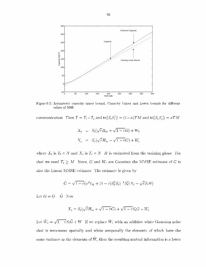
92

0 50 100 150 200 250 300 350 400−50

0

50

100

150

200

250

300

350

SNR (dB)

Cap

acity

(bi

ts/T

)

Coherent Capacity

Training Lower Bound

Capacity

Figure 6.2: Asymptotic capacity upper bound, Capacity Upper and Lower bounds for di�erentvalues of SNRcommunication. Then T = Tt+Tc and trfStSyt g = (1��)TM and trfScSycg = �TM .Xt = St(prHm +p1� rG) +WtXc = Sc(prHm +p1� rG) +Wcwhere Xt is Tt � N and Xc is Tc � N . H is estimated from the training phase. Forthat we need Tt � M . Since, G and Wt are Gaussian the MMSE estimate of G isalso the Linear MMSE estimate. The estimate is given byG = p1� r(�2IM + (1� r)SytSt)�1Syt (Xt �prStH)Let �G = G� G. NowXc = St(prHm +p1� rG) +p1� rSt �G +WcLet Wc = p1� rSt �G +W . If we replace Wc with an additive white Gaussian noisethat is zero-mean spatially and white temporally the elements of which have thesame variance as the elements of Wc then the resulting mutual information is a lower

93bound to the actual mutual information in the above channel. This is stated formallyin the following proposition.Proposition VI.5 (Theorem 1 in [33]). LetX = SH +Wbe a rician fading channel with H known to the receiver. Let S and W satisfy1ME[SSy] = 1 and 1ME[WW y] = �2 and be uncorrelated with each other. Thenthe worst case noise has i.i.d. zero mean Gaussian distribution, W � CN (0; IN).Moreover, this distribution has the following minimax propertyIW�CN (0;�2IN );S(X;S) � IV�CN (0;�2IN );S�CN (0;IM )(X;S) � IV;S�CN (0;IM)(X;S)The variance of the elements of Wc is given by�2wc = �2 + 1� rNTc trfE[ �G �Gy]�TIMg= �2 + (1� r)�TMTc 1NME[ �G �Gy]= �2 + (1� r)�TMTc �2�Gand the lower bound isCt � T � TtT E log det�IM + �effM H1�Hy1�where �eff is the ratio of the energies in the elements of ScH and energies in theelements of Wc and H1 = prnewHm +p1� rnewG where rnew = rr+(1�r)�2G . � is theoptimum signal correlation matrix the form of which depends on the distribution ofH1. This problem has been solved when H1 is a rician channel for low values of �effand high values of �eff with M � N in section 6.3.1.

94To calculate �eff , the energy in the elements of SH is given by�2SH = 1NTc [rtrfHmHym�TIMg+ (1� r)trfGGy�TIMg]= �TMTc 1NM [rNM + (1� r)trfGGyg]= �TMTc [r + (1� r)�2G]which gives us �eff = �T�[r + (1� r)�2G]Tc + (1� r)�T��2�G6.4.1 Optimization of St, � and TtWe will optimize St, � and Tt to maximize the lower bound. In this section wemerely state the main results and their interpretations. Derivations and details aregiven in the Appendices.Optimization over St is not very practical as St e�ects the distribution of H, theform of � as well as �eff . To make the problem simpler we will just �nd the valueof St that maximizes �eff .Theorem VI.8. The signal St that maximizes �eff satis�es the following conditionSytSt = (1� �)TIMProof: See Appendix .11.Optimizing over St gives�eff = �T�[Mr + �(1� �)T ]Tc(M + �(1� �)T ) + (1� r)�T�Mand the corresponding lower bound is given byCt � T � TtT E log det�IM + �effM H1�Hy1�

95where �eff is as given above and H1 = prnewHm + p1� rnewG where rnew =r 1+(1�r)(1��) �M Tr+(1�r)(1��) �M T and G is a matrix consisting of i.i.d. Gaussian circular randomvariables with mean zero and unit variance. Now, � is the input signal covariancematrix when the channel is rician and known to the receiver. The form of � is knownto us for �eff ! 0 and �eff !1.Optimization over � is straighforward as � a�ects the lower bound only through�eff and can be stated in the following proposition.Theorem VI.9. The optimal power allocation � in a training based scheme is givenby � = 8>>>>><>>>>>: minf �p ( � 1� �); 1g for Tc > (1� r)Mminf12 + rM2T� ; 1g for Tc = (1� r)Mminf +p ( � 1� �); 1g for Tc < (1� r)Mwhere = MTc+T�TcT�[Tc�(1�r)M ] and � = rMT� . The corresponding lower bound is given byCt � T � TtT E log det�IM + �effM H1�Hy1�where for Tc > (1� r)M�eff = 8><>: T�Tc�(1�r)M (p �p � 1� �)2 when � = �p ( � 1� �)r�1+(1�r)� when � = 1for Tc = (1� r)M�eff = 8><>: T 2�24(1�r)M(M+T�) (1 + rMT� )2 when � = 12 + rM2T�rT�(1�r)(M+T�) when � = 1and for Tc < (1� r)M�eff = 8><>: T�(1�r)M�Tc (p� �p� + 1 + �)2 when � = +p ( � 1� �)r�1+(1�r)� when � = 1

96and rnew is given by substituting the appropriate value of � in the expressionr1 + (1� r)(1� �) �MTr + (1� r)(1� �) �MTProof: See Appendix .12.For optimization over Tt we draw somewhat similar conclusions as in [33]. Weshow that Tt = M is the optimal setting for \large" SNR and Tt = 0 for smallSNR. The intuition is that increasing Tt linearly decreases the capacity through theterm (T � Tt)=T , but only logarithmically increases the capacity through the highere�ective SNR �eff [33]. Therefore, it makes sense to make Tt as small as possible.For small SNR we show that � = 1. It is clear that optimization of Tt makes senseonly when � is strictly less than 1. When � = 1 no power is devoted to training andTt can be made as small as possible which is zero. When � < 1 the smallest value Ttcan be is M since it takes alteast that many intervals to completely determine theunknowns.Theorem VI.10. The optimal length of the training interval is Tt = M whenever� < 1 for all values of � and T , and the capacity lower bound isCt � T �MT E log det�IM + �effM H1�Hy1� (6.7)where �eff = 8>>>>><>>>>>: T�T�(2�r)M (p �p � 1� �)2 for T > (2� r)MT 2�24(1�r)M(M+T�)(1 + rMT� )2 for T = (2� r)MT�T�(2�r)M (p� �p� + 1 + �)2 for T < (2� r)MThe optimal power allocations are easily obtained from Theorem VI.9 by simply set-ting Tc = T �M .Proof: See Appendix .13

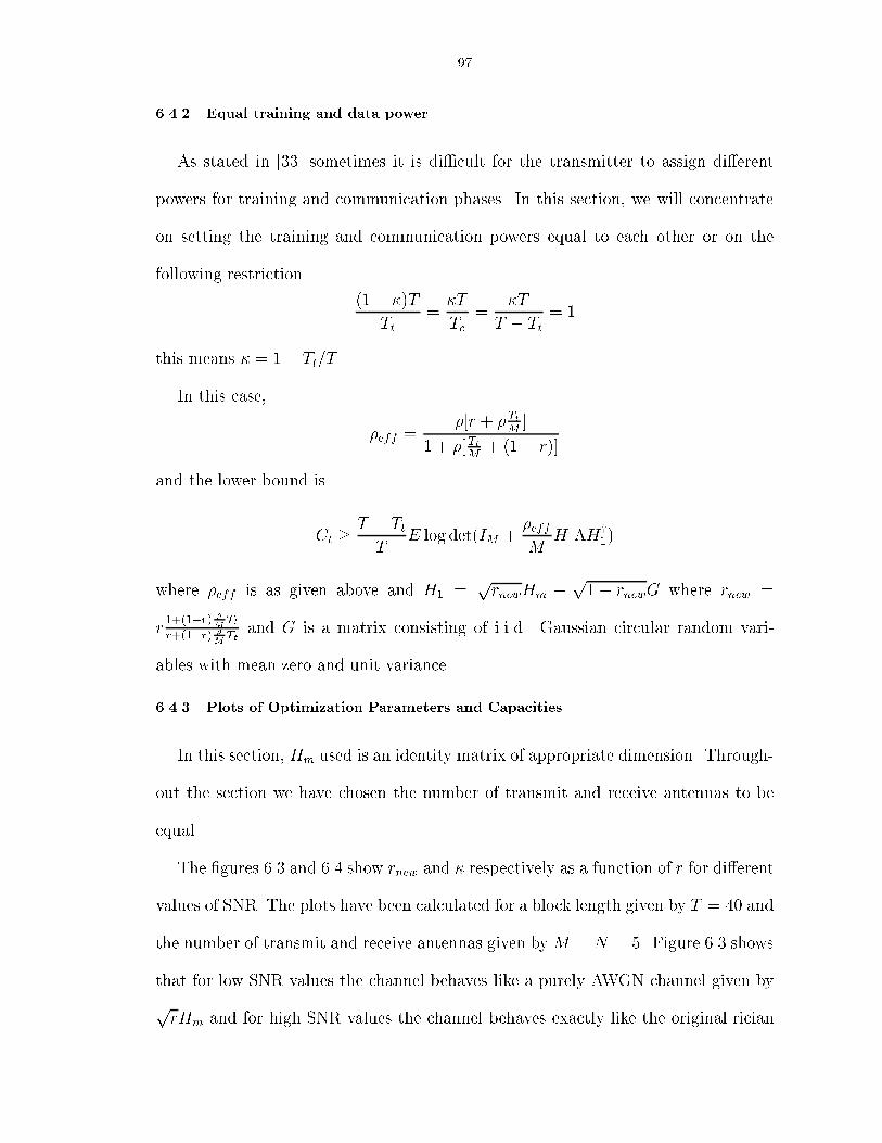
976.4.2 Equal training and data powerAs stated in [33] sometimes it is di�cult for the transmitter to assign di�erentpowers for training and communication phases. In this section, we will concentrateon setting the training and communication powers equal to each other or on thefollowing restriction (1� �)TTt = �TTc = �TT � Tt = 1this means � = 1� Tt=T .In this case, �eff = �[r + � TtM ]1 + �[ TtM + (1� r)]and the lower bound isCt � T � TtT E log det(IM + �effM H1�Hy1)where �eff is as given above and H1 = prnewHm + p1� rnewG where rnew =r 1+(1�r) �M Ttr+(1�r) �M Tt and G is a matrix consisting of i.i.d. Gaussian circular random vari-ables with mean zero and unit variance.6.4.3 Plots of Optimization Parameters and CapacitiesIn this section, Hm used is an identity matrix of appropriate dimension. Through-out the section we have chosen the number of transmit and receive antennas to beequal.The �gures 6.3 and 6.4 show rnew and � respectively as a function of r for di�erentvalues of SNR. The plots have been calculated for a block length given by T = 40 andthe number of transmit and receive antennas given byM = N = 5. Figure 6.3 showsthat for low SNR values the channel behaves like a purely AWGN channel given byprHm and for high SNR values the channel behaves exactly like the original rician

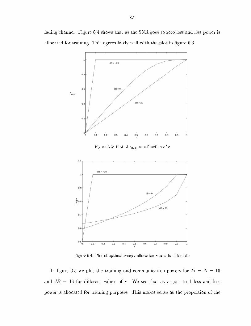
98fading channel. Figure 6.4 shows that as the SNR goes to zero less and less power isallocated for training. This agrees fairly well with the plot in �gure 6.3.

0 0.1 0.2 0.3 0.4 0.5 0.6 0.7 0.8 0.9 10

0.2

0.4

0.6

0.8

1

r

dB = 20

dB = 0

dB = −20

r new

Figure 6.3: Plot of rnew as a function of r

0 0.1 0.2 0.3 0.4 0.5 0.6 0.7 0.8 0.9 10.5

0.6

0.7

0.8

0.9

1

1.1

r

kapp

a

dB = 20

dB = 0

dB = −20

Figure 6.4: Plot of optimal energy allocation � as a function of rIn �gure 6.5 we plot the training and communication powers for M = N = 10and dB = 18 for di�erent values of r. We see that as r goes to 1 less and lesspower is allocated for training purposes. This makes sense as the proportion of the

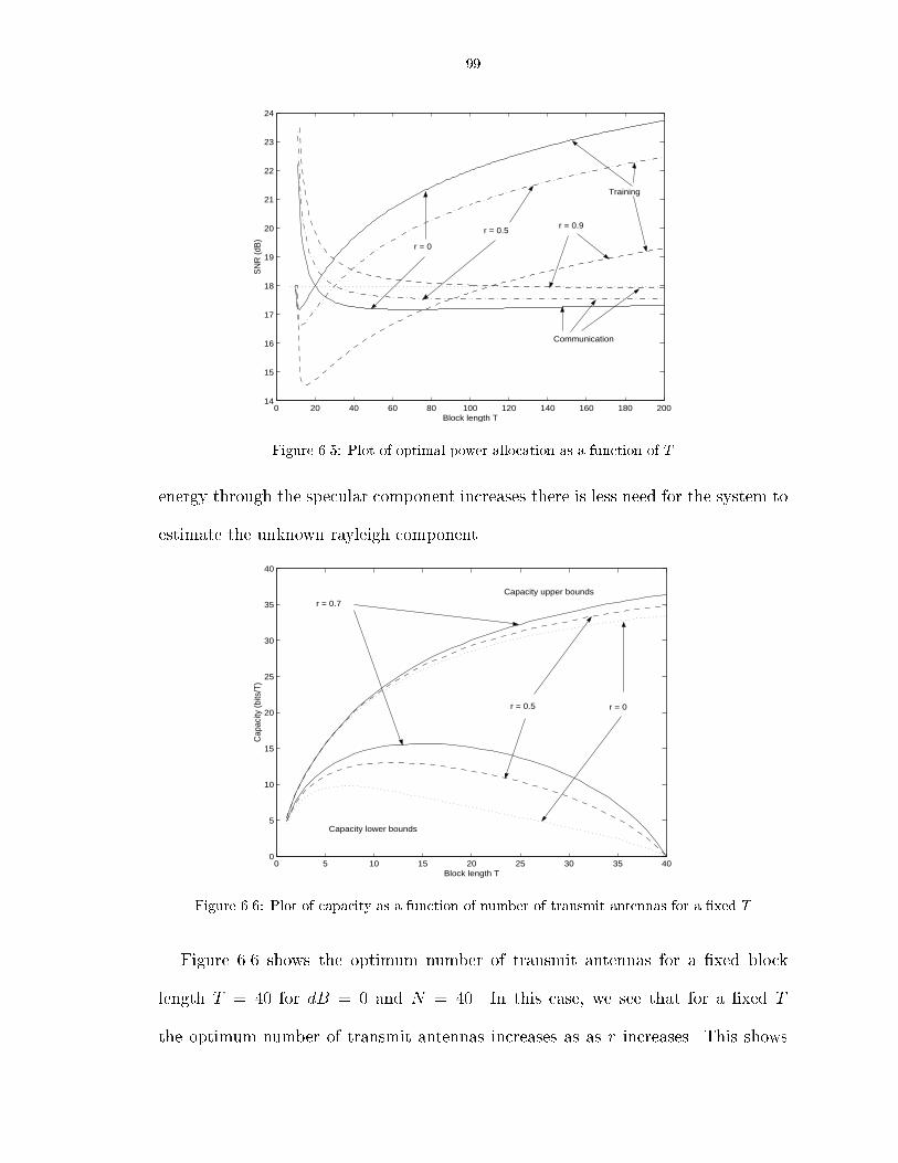
99

0 20 40 60 80 100 120 140 160 180 20014

15

16

17

18

19

20

21

22

23

24

Block length T

SN

R (d

B)

r = 0

r = 0.5 r = 0.9

Training

Communication

Figure 6.5: Plot of optimal power allocation as a function of Tenergy through the specular component increases there is less need for the system toestimate the unknown rayleigh component.

0 5 10 15 20 25 30 35 400

5

10

15

20

25

30

35

40

Block length T

Cap

acity

(bits

/T)

r = 0 r = 0.5

r = 0.7

Capacity lower bounds

Capacity upper bounds

Figure 6.6: Plot of capacity as a function of number of transmit antennas for a �xed TFigure 6.6 shows the optimum number of transmit antennas for a �xed blocklength T = 40 for dB = 0 and N = 40. In this case, we see that for a �xed Tthe optimum number of transmit antennas increases as as r increases. This shows

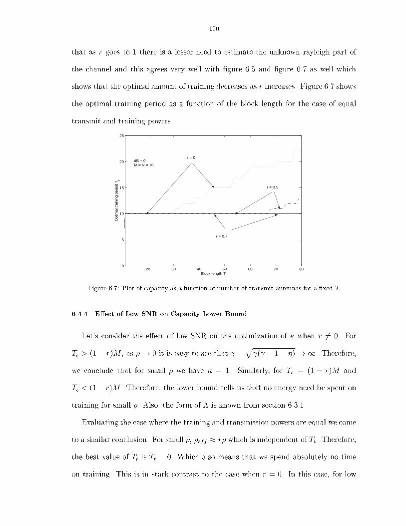
100that as r goes to 1 there is a lesser need to estimate the unknown rayleigh part ofthe channel and this agrees very well with �gure 6.5 and �gure 6.7 as well whichshows that the optimal amount of training decreases as r increases. Figure 6.7 showsthe optimal training period as a function of the block length for the case of equaltransmit and training powers.

20 30 40 50 60 70 800

5

10

15

20

25

Block length T

Opt

imal

trai

ning

per

iod

T t

r = 0.7

r = 0

r = 0.5

dB = 0M = N = 10

Figure 6.7: Plot of capacity as a function of number of transmit antennas for a �xed T6.4.4 E�ect of Low SNR on Capacity Lower BoundLet's consider the e�ect of low SNR on the optimization of � when r 6= 0. ForTc > (1� r)M , as �! 0 it is easy to see that �p ( � 1� �)!1. Therefore,we conclude that for small � we have � = 1. Similarly, for Tc = (1 � r)M andTc < (1� r)M . Therefore, the lower bound tells us that no energy need be spent ontraining for small �. Also, the form of � is known from section 6.3.1.Evaluating the case where the training and transmission powers are equal we cometo a similar conclusion. For small �, �eff � r� which is independent of Tt. Therefore,the best value of Tt is Tt = 0. Which also means that we spend absolutely no timeon training. This is in stark contrast to the case when r = 0. In this case, for low

101SNR Tt = T=2 [33] and �eff behaves as O(�2).Note that in both cases of equal and unequal power distribution between trainingand communication phases we have the signal distribution during data transmissionphase to be Gaussian. Therefore, the lower bound behaves as r��maxfHmHymg. Also,rnew = 1 for small � showing that the channel behaves as a purely Gaussian channel.All the conclusions above mimic those of the capacity results with Gaussian inputin section 6.3.3. The low SNR non-coherent capacity results for the case of a Gaussianinput tell us that the capacity behaves as r��max with Gaussian input. Moreover,the results in [33] also agree quite well the results derived in section 6.3.3. We showedthat for purely rayleigh fading channels with Gaussian input the capacity behaves as�2 which is what the lower bound results in [33] also show. This makes sense becausethe capacity lower bound assumes that the signaling input during communicationperiod is Gaussian. This shows that the lower bound derived in [33] and extendedhere is quite tight for low SNR values.6.4.5 E�ect of High SNR on Capacity Lower BoundFor high SNR, becomes TcTc�(1�r)M and the optimal power allocation � becomes� = pTcpTc +p(1� r)Mand �eff = T(pTc +p(1� r)M)2�In the case of equal training and transmit powers, we have for high ��eff = � TtTt +M(1� r)For high SNR, the channel behaves as if it is completely known to the receiver.Note that in this case rnew = r and � is an identity matrix for the case M � N .

102From the expressions for �eff given above we conclude that unlike the case of lowSNR the value of r a�ects the amount of time and power devoted for training.Let's look at the capacity lower bound for high SNR. The optimizing � in thisregime is an identity matrix. We know that at high SNR the optimal training periodis M therefore, the resulting lower bound is given byCt � T �MT E log det0BBB@IM + ��q1� MT +q (1�r)MT �2HHyM 1CCCANote that the lower bound has H �guring in it instead of H1. That is so because forhigh SNR, rnew = r. This lower bound can be optimized over the number of transmitantennas used in which case the lower bound can be rewritten asCt � maxM 0�M maxn�0BBBB@ MM 0 1CCCCA T �M 0T E log det0BBB@IM 0 + ��q1� M 0T +q (1�r)M 0T �2HnHynM 0 1CCCAwhere now Hn is the nth matrix out of a possible M choose M 0 (the number ofways to choose M 0 transmit elements out of a maximum M elements) matrices ofsize M 0 � N . Let Q = minfM 0; Ng and �i be an arbitrary nonzero eigenvalue of1�q1�M0T +q (1�r)M0T �2 HnHynM 0 then we haveCt � maxM 0�M maxn�0BBBB@ MM 0 1CCCCA�1� M 0T � QXi=1 E log(1 + ��i)At high SNR, the leading term involving � inPQi=1E log(1+ ��i) is Q log � which isindependent of n. Therefore,Ct � maxM 0�M8><>: (1� M 0T )M 0 log � if M 0 � N(1� M 0T )N log � if M > N

103The expression (1�M 0T )M 0, is maximized by choosingM 0 = T=2 when minfM;Ng �T=2 and by choosing M 0 = minfM;Ng when minfM;Ng � T=2. This means thatthe expression is maximized whenM 0 = minfM;N; T=2g. This is a similar conclusiondrawn in [33] and [74]. Also, the leading term in � for high SNR in the lower boundis given by Ct � (1� KT )K log �where K = minfM;N; T=2g. This result suggests that the number of degrees offreedom available for communication is limited by the minimum of the number oftransmit antennas, receive antennas and half the coherence interval. Moreover, fromthe results in section 6.3.4 we see that the lower bound is tight for the case whenM � N and large T in the sense that the leading term involving � in the lower boundis the same as the one in the expression for capacity.6.4.6 Comparison of the training based lower bound (6.7) with the lower boundderived in section 6.3.2It is quite conceivable to use the lower bound to training based techniques as thelower bound to the overall capacity of the system. Actually, using this \training"based lower bound it can be shown that the capacity as T ! 1 converges to thecapacity as if the receiver knows the channel. We will see how the new lower boundderived in this work compares with this training based lower bound. The three�gures below show that the new lower bound is indeed useful as it does better thanthe training based lower bound for r = 0. The plots are for M = N = 1 for di�erentvalues of SNR.However, we note that for r = 1 the training based lower bound and the lowerbound derived in section 6.3.2 agree perfectly with each other and are equal to theupper bound.

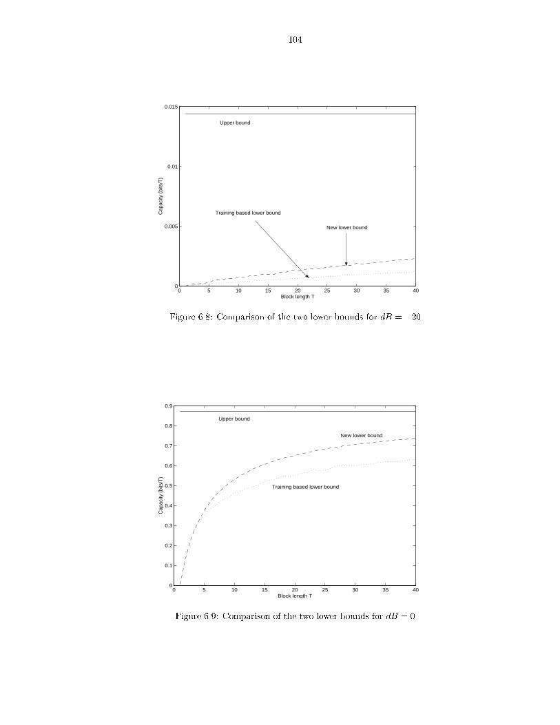
104

0 5 10 15 20 25 30 35 400

0.005

0.01

0.015

Block length T

Cap

acity

(bi

ts/T

)

Upper bound

New lower bound

Training based lower bound

Figure 6.8: Comparison of the two lower bounds for dB = �20

0 5 10 15 20 25 30 35 400

0.1

0.2

0.3

0.4

0.5

0.6

0.7

0.8

0.9

Block length T

Cap

acity

(bits

/T)

Upper bound

Training based lower bound

New lower bound

Figure 6.9: Comparison of the two lower bounds for dB = 0

105

0 5 10 15 20 25 30 35 400

1

2

3

4

5

6

Block length T

Cap

acity

(bits

/T)

Upper bound

Training based lower bound

New lower bound

Figure 6.10: Comparison of the two lower bounds for dB = 206.5 Conclusions and Future WorkIn this chapter, we have analyzed the standard rician fading channel for capacity.Most of the analysis was for a general specular component but, for the special caseof a rank-one specular component we were able to show more structure on the signalinput. For the case of general specular component, we were able to derive asymptoticclosed form expressions for capacity for low and high SNR scenarios.A big part of the analysis e.g. the non-coherent capacity expression and trainingbased lower bounds can be very easily extended to the non-standard rician modelsconsidered in the previous two chapters.One important result of the analysis is that for low SNRs beamforming is verydesirable whereas for high SNR scenarios it is not. This result is very useful in de-signing space-time codes. For high SNR scenarios, one could wager that the standardcodes designed for rayleigh fading can work for the case of rician fading as well.A lot more work needs to be done such as for case of M > N . We believe that

106more work along the lines of [74] is possible for the case of rician fading. We concludeas in [74] that at least for the case M = N the number of degrees of freedom is givenby M T�MT . The training based lower bound gives an indication that the number ofdegrees of freedom of a rician channel is the same as that of a rayleigh fading channelminfM;N; T=2g (derived in [74] and [33]). It also seems reasonable that the work in[4] can be extened to the case of rician fading.

APPENDICES

107

108.1 Derivation of Stability Condition (3.6)We will follow the Z-transform method of [37]. Let ~�(z) donate the Z-transformof �k and ~Gi(z) donate the Z-transform of the ith component of Gk. Then we havethe following ~�(z) = �min 11� z�1 + NXi=1 ~Gi(z)~Gi(z) = (1� 2�P �i + 2�2P �2i ) ~Gi(z) + �2P �2i z�1 ~�(z) +Gi(0)which leads to ~�(z) = �min 11�z�1 +PNi=1 Gi(0)1�z�1(1� 2�P �i+ 2�2P �2i )1�PNi=1 �2P �2i z�11�z�1(1� 2�P �i+ 2�2P �2i ) (.8)and ~Gi(z) = 1D(z) �2P �2iN(z) +Gi(0)D(z)1� z�1(1� 2�P �i + 2�2P �2i ) (.9)where N(z) and D(z) denote the numerator and the denominator in (.8). Therefore,the condition for stability is that the roots ofz � (1� 2�P �i + 2�2P �2i )for i = 1; : : : ; N and QNi=1 hz � (1� 2�P �i + 2�2P �2i )i�PNi=1 �2P �2i Qk 6=i hz � (1� 2�P �k + 2�2P �2k)ishould lie within the unit circle.Please note that (.9) should be used to determine the stability of ~Gi(z) and not~Gi(z) = �2P �2i z�1 h�min 11�z�1 +Pk 6=i ~Gk(z)i +Gi(0)1� z�1(1� 2�P �i + 3�2P �2i )

109that was used in [37].Following the rest of the procedure as outlined in [37] exactly, we obtain theconditions for stability to be (3.6)..2 Derivation of expression (3.8)Here we follow the procedure in [20]. Assuming Gk converges we have the expres-sion for G1 to beG1 = P [2��� 2�2�� �2�211T ]�1�2P �21�minThen we have Gk+1 �G1 = F (Gk �G1)where F = I � 2�P � + 2�2P � + �2P �211T . Since �k = trfGkg we have1Xk=0(�k � �1) = trf 1Xk=0(Gk �G1)g= trf 1Xk=0 F k(G0 �G1)g= trf(I � F )�1(G0 �G1)gfrom which (3.8) follows..3 Derivation of the misadjustment factor (3.7)Here we follow the approach of [37]. The misadjustment factor is de�ned asM(�) = �1��min�min . Since �1 = limz!1(1� z�1)~�(z) we have�1 = limz!1 ��min + (1� z�1)PNi=1 Gi(0)1�z�1(1� 2�P �i+ 2�2P �2i )�limz!1 �1�PNi=1 �2P �2i z�11�z�1(1� 2�P �i+ 2�2P �2i )�

110That is �1 = �min1� 12PNi=1 ��i1���i= �min1� �(�)from which 3.7 follows..4 Proof of Theorem III.1 in Section 3.5.1For the proof, we need some de�nitions �rst. We de�ne for p � 1 the set Mp ofF = fFig as Mp = �F : supi kS(T )i kp = o(T ); as T !1� (.10)where S(T )i =P(i+1)T�1j=iT (Fj � E[Fj]).The proof is just a slightly modi�ed version of the proof to Theorem 2 derived inSection IV in [45, pp. 766-769]. The modi�cation takes into account that Fk is nolonger Fk = XkXHk but, Fk = IkXkXHk . The Theorem III.1 is proved in a step bystep manner using di�erent lemmas. First, we rewriteXk = 1Xj=�1 aj�(k; j) + �k; 1Xj=�1aj <1where by de�nitionaj def= supk kA(k; j)k; �(k; j) = a�1j A(k; j)�k�jThe new process has some simple properties as listed in [45].Lemma .6. if fGkg is a �-mixing d�d-dimensional matrix then so is fFk = IkGkg.Lemma .7. Let fFkg be a �-mixing d � d-dimensional matrix process with mixingrate f�(m). Thensupi kS(T )i k2 � 2cd(T T�1Xm=0p�(m))1=2 ; 8T � 1

111where S(T )i is as de�ned earlier and c is de�ned by c def= supi kFi � EFik2.Proof: Proof is the same as the proof of Lemma 1 in [45].Lemma .8. Let Fk = IkXkXHk , where fXkg is de�ned by (3.11) with supk k�kk4 <1. Then fFkg 2 M2, where M2 is de�ned by (.10).Proof: Proof is practically the same as the proof for Lemma 2 in [45]. All we needto say is that if fGkg is �-mixing then so is fIkGkg.Lemma .9. Let supk EkXkk2 < 1. Then fIkXkXHk g 2 S if and only if (3.13)holds, where S is de�ned by (3.10).Proof: Let us �rst assume that (3.13) is true. Take �� = (1 + supk EkXkk2)�1.Then applying Theorem 2.1 in [32] to the deterministic sequence Ak = �E[IkXkXHk ]for any � 2 (0; ��], it is easy to see that fIkXkXHk g 2 S(��).Conversely, if fXkXHk g 2 S, then there exists �� 2 (0; (1 + supk EkXkk2)�1] suchthat fXkXHk g 2 S(��). Now, applying Theorem 2.2 in [32] to the deterministicsequence Ak = ��E[IkXkXHk ], it is easy to see that (3.13) holds. This completes theproof.Lemma .10. Let Fk = IkXkXHk , where fXkg is de�ned by (3.11) with (3.12) satis-�ed. Then fFkg satis�es condition 1) of Theorem 1.Proof: From Lemma 4 in [45] we know that Gk = XkXHk satis�es condition 1) ofTheorem 1. Since kFkk � kGkk it follows that fFkg satis�es condition 1) of Theorem1.Lemma .11 (Lemma 5 in [45]). Let fzkg be a nonnegative random sequence suchthat for some a > 0; b > 0 and for all i1 < i2 < : : : < in, 8n � 1E exp( nXk=1 zik) � expfan+ bg (.11)

112Then for any L > 0 and any n � i � 0E exp(12 nXj=i+1 zjI(zj � L)) � expfea�L=2(n� i) + bgwhere I(�) is the indicator function.Proof: This lemma has been proved in [45].Lemma .12. Let Fk = IkXkXHk where fXkg is de�ned by (3.11) with (3.12) satis-�ed. Then fFkg satis�es condition 2) of Theorem 1.Proof: Set for any �xed k and lzj def= zj(k; l) = (j+1)T�1Xt=jT [It�(t; k)�(t; l)H � EIt�(t; k)�(t; l)H ] Then, we havenXj=i+1 kS(jT )k � 1Xk;l=�1akal nXj=i+1 zj + 2 1Xk=�1ak nXj=i+1 (j+1)T�1Xt=jT It�(t; k)�Ht (.12)We �rst consider the second to the last term in the previous equation. By theHolder inequalityE exp(� 1Xk;l=�1akal nXj=i+1 zj) � 1Yk;l=�1(E exp(�A2 nXj=i+1 zj))akalA2where A def= P1j=�1 aj.Now, let c =Pk Ek�kk2, and note thatkIt�(t; k)�(t; l)Hk � k�(t; k)�(t; l)Hk� 12[k�(t; k)k2 + k�(t; l)k2]� 12(k�t�kk2 + k�t�lk2)and we have zj � 12 (j+1)T�1Xt=jT (k�t�kk2 + k�t�lk2) + cmT

113By this and (3.12) it is easy to prove that the sequence f�zjg satsi�es (.11) witha = (K + c=m)T and b = logM , where � is de�ned as in (3.12). Consequently, byLemma 5 in [45] we have for any L > 0E exp(�2 nXj=i+1 zjI(zj � LT )) �M expne(K+c��L2 )T (n� i)oNow, in view of the above, taking � < �A�24 and L > 2��1(K + c), and applyingthe Holder inequality, we haveE exp(2�A2 nXj=i+1 zjI(zj � LT )) � Mexpf��(T )(n� i)gwhere �(T )! 0 as T !1, which is de�ned by�(T ) = 4��1A2 exp�(K + c� �L2 )T�Next, we consider the term xj def= zjI(zj � LT ).By the inequality ex � 1 + 2x, 0 � x � log 2, we have for small � > 0exp(2�A2 nXj=i+1xj) � nYj=i+1(1 + 4�A2xj)As noted before, for any �xed k and l, the process f�(t; k)�(t; l)Hg is �-mixingwith mixing rate �(m� jk � lj). Consequently, for any �xed k and l, both fzjg andfxjg are also �-mixing with mixing rate �((m � 1)T + 1 � jk � lj). Note also thatby Lemma 1 in [45]Exj � Ezj � kzjk2 � fkl(T ) where fkl(T ) = 2cdnTPT�1m=0p�(m� jk � jj)o 12Therefore, applying Lemma 6.2 in [45], we haveE nYj=i+1(1 + 4�A2xj) � 2f1 + 8�A2[fkl(T ) + 2LT�(T + 1� jk � lj)]gn�i� 2 expf8�A2[fkl(T ) + 2LT�(T + 1� jk � lj)](n� i)g

114Finally, using the Schwarz inequality we getE exp(�A2 nXj=i+1 zj) � (E exp(2�A2 nXj=i+1 zjI(zj � LT )))1=2 �(E exp(2�A2 nXj=i+1xj))1=2� p2M expf�[�(T ) + 8A2fkl(T ) +16LTA2�(T + 1� jk � lj)](n� i)gTherefore, it is not di�cult to see that there exists a function g(T ) = o(T ) suchthat for all small � > 0E exp(� 1Xk;l=�1akal nXj=i+1 zj) � p2M expf�g(T )(n� i)g:We can similarly bound the second term in (.12) and we are done.Now we will highlight some of the remarks and corollaries to Theorem 2 in [45].The remarks and corollaries and pertinent to this Theorem too.Remark .1. By taking A(k; 0) = I, A(k; j) = 0, 8k; 8j 6= 0, and �k = 0, 8kin (3.11), we see that fXkg is the same as �k, which means that Theorem III.1 isapplicable to any �-mixing sequences.Corollary .3. Let the signal process be generated by (3.11), where f�kg is a boundeddeterministic sequence, and f�kg is an independent sequence satisfyingsupk E[exp(�k�kk2)] <1; for some � > 0Then fXkXHk g 2 Sp for some p � 1 if and only if there exists an integer h > 0 anda constant � > 0 such that (3.13) holds.Proof: Similar to the proof of Corollary 1 in [45].

115.5 Derivation of Expressions in Section 3.7.2In this section, we will need the following identity1Xs=0 s(1� ��)2s = (1� ��)2�2�2(2� ��)2First, we have the following expressions for LMSJ0k+1 = kXs=0(1� ��2)k�sXsnsJ1k+1 = � kXs=0(1� ��2)k�s�1D1(k; s+ 1)XsnsJ2k+1 = �2 kXs=0(1� ��2)k�s�2D2(k; s+ 1)Xsnswhere D1(k; s) = kXu=s Zu k � s D1(k; s) = 0 s > kD2(k; s) = kXu=sD1(k; u+ 1)Zuand Zu = E[XuXHu ]�XuXHuThis leads tolimk!1E[J0k+1(J0k+1)H ] = limk!1�2v kXs=0(1� ��2)2(k�s)E[X0XH0 ]and the expression follows.limk!1E[J0k+1(J1k+1)H ] = ��2v kXs=0(1� ��2)2s�1E[D1(s; 1)X0XH0 ]Now, E[ZuX0XH0 ] = E[XuXHu ]E[X0XH0 ]� E[XuXHu X0XH0 ] = 0 which givesE[D1(s; 1)X0XH0 ] = 0

116limk!1E[J1k+1(J1k+1)H ] = �2v�2 1Xu=0(1� ��2)2u�2E[D1(u; 1)X0XH0 D1(u; 1)H]Now E[ZvX0XH0 ZHu ] = �6I � �2E[XvXHv X0XH0 ]� �2E[X0XH0 XuXHu ] +E[XvXHv X0XH0 XuXHu ]= 0 if v 6= u= N�6I if v = u

Therefore, E[D1(u; 1)X0XH0 D1(u; 1)H] = uN�6I and the expression follows.limk!1E[J0k+1(J2k+1)H ] = �2�2vP1s=0E[D2(s; 1)X0XH0 ]. NowE[ZvZuX0XH0 ] = �6I � �2E[XvXHv X0XH0 ]� �2E[XuXHu X0XH0 ] +E[XvXHv XuXHu X0XH0 ]= 0 if v 6= uTherefore, E[D2(s; 1)X0XH0 ] = 0.Second, we have the following expressions for SPULMSJ0k+1 = kXs=0(1� �P �2)k�sIsXsnsJ1k+1 = � kXs=0(1� �P �2)k�s�1D1(k; s+ 1)IsXsnsJ2k+1 = �2 kXs=0(1� �P �2)k�s�2D2(k; s+ 1)IsXsns

117where D1(k; s) = kXu=s Zu k � s D1(k; s) = 0 s > kD2(k; s) = kXu=sD1(k; u+ 1)Zuand Zu = IuXuXHu � 1PE[XuXHu ]This leads tolimk!1E[J0k+1(J0k+1)H ] = limk!1�2v kXs=0(1� ��2)2(k�s)E[I0X0XH0 I0]and the expression follows.limk!1E[J0k+1(J1k+1)H ] = ��2v kXs=0(1� ��2)2s�1E[D1(s; 1)I0X0XH0 I0]Now, E[ZuI0X0XH0 I0] = E[IuXuXHu ]E[I0X0XH0 I0] � E[IuXuXHu I0X0XH0 I0] = 0which gives E[D1(s; 1)X0XH0 ] = 0.limk!1E[J1k+1(J1k+1)H ] = �2v�2 1Xu=0(1� ��2)2u�2E[D1(u; 1)I0X0XH0 I0D1(u; 1)H]NowE[ZvI0X0X0I0ZHu ] = �6I � �2E[IvXvXHv I0X0XH0 I0]� �2E[I0X0XH0 I0XuXHu Iu]+E[IvXvXHv I0X0XH0 I0XuXHu Iu]= 0 if v 6= u= (N + 1)P � 1P 3 �6I if v = u

Therefore, E[D1(u; 1)X0XH0 D1(u; 1)H] = u (N+1)P�1P 3 �6I and the expression follows.

118limk!1E[J0k+1(J2k+1)H ] = �2�2vP1s=0E[D2(s; 1)X0XH0 ]. NowE[ZvZuX0XH0 ] = �6I � �2E[IvXvXHv I0X0XH0 I0]� �2E[IuXuXHu I0X0XH0 I0]+E[IvXvXHv IuXuXHu I0X0XH0 I0]= 0 if v 6= uTherefore, E[D2(s; 1)X0XH0 ] = 0..6 Derivation of Expressions in Section 3.7.1In this section, we will need the following identitiessXv;w=1 a2jv�wj = s(1� a4)� 2a2 + 2a2(s+1)(1� a2)2sXv;w=1 ajv�wjav+w = a2(1� a2)2 [1 + a2 � (2s+ 1)a2s + (2s� 1)a2s+2]1Xs=0 s(1� ��)2s = (1� ��)2�2�2(2� ��)2First, we have the following expressions for LMSJ0k+1 = kXs=0(1� �)k�sXsnsJ1k+1 = � kXs=0(1� �)k�s�1D1(k; s+ 1)XsnsJ2k+1 = �2 kXs=0(1� �)k�s�2D2(k; s+ 1)Xsnswhere D1(k; s) = kXu=s Zu k � s D1(k; s) = 0 s > kD2(k; s) = kXu=sD1(k; u+ 1)Zuand Zu = E[XuXHu ]�XuXHu

119This leads tolimk!1E[J0k+1(J0k+1)H ] = limk!1�2v kXs=0(1� �)2(k�s)E[X0XH0 ]and the expression follows.limk!1E[J0k+1(J1k+1)H ] = ��2v kXs=0(1� �)2s�1E[D1(s; 1)X0XH0 ]Now, E[ZuX0XH0 ] = E[XuXHu ]E[X0XH0 ] � E[XuXHu X0XH0 ] = � NP 3�2u which givesE[D1(s; 1)X0XH0 ] = � NP 3�2 1��2s1��2 .limk!1E[J1k+1(J1k+1)H ] = �2v�2 1Xu=0(1� �)2u�2E[D1(u; 1)X0XH0 D1(u; 1)H]NowE[ZvX0XH0 ZHu ] = I � E[XvXHv X0XH0 ]� E[X0XH0 XuXHu ] + E[XvXHv X0XH0 XuXHu ]= [(N2 + 1)�v+u�jv�uj +N�2jv�ujTherefore,E[D1(u; 1)X0XH0 D1(u; 1)H] = (N2 + 1) uXs=1 uXt=1 �jv�uj�v+u +N uXs=1 uXt=1 �2jv�ujand the expression follows.limk!1E[J0k+1(J2k+1)H ] = �2�2vP1s=0E[D2(s; 1)X0XH0 ]. NowE[ZvZuX0XH0 ] = I � E[XvXHv X0XH0 ]� E[XuXHu X0XH0 ] + E[XvXHv XuXHu X0XH0 ]= [(N2 + 1)�v+u�jv�uj +N�2jv�ujTherefore,E[D2(s; 1)X0XH0 ] = (N2 + 1) uXs=1 uXt=s+1�jv�uj�v+u +N uXs=1 uXt=s+1 �2jv�uj

120Second, we have the following expressions for SPULMSJ0k+1 = kXs=0(1� �P )k�sIsXsnsJ1k+1 = � kXs=0(1� �P )k�s�1D1(k; s+ 1)IsXsnsJ2k+1 = �2 kXs=0(1� �P )k�s�2D2(k; s+ 1)IsXsnswhere D1(k; s) = kXu=s Zu k � s D1(k; s) = 0 s > kD2(k; s) = kXu=sD1(k; u+ 1)Zuand Zu = IuXuXHu � 1PE[XuXHu ]This leads tolimk!1E[J0k+1(J0k+1)H ] = limk!1�2v kXs=0(1� �)2(k�s)E[I0X0XH0 I0]and the expression follows.limk!1E[J0k+1(J1k+1)H ] = ��2v kXs=0(1� �)2s�1E[D1(s; 1)I0X0XH0 I0]Now, E[ZuI0X0XH0 I0] = E[IuXuXHu ]E[I0X0XH0 I0]�E[IuXuXHu I0X0XH0 I0] = � NP 3�2uwhich gives E[D1(s; 1)X0XH0 ] = � NP 3�2 1��2s1��2 .limk!1E[J1k+1(J1k+1)H ] = �2v�2 1Xu=0(1� �)2u�2E[D1(u; 1)I0X0XH0 I0D1(u; 1)H]

121NowE[ZvI0X0X0I0ZHu ] = I � E[IvXvXHv I0X0XH0 I0]� E[I0X0XH0 I0XuXHu Iu]+E[IvXvXHv I0X0XH0 I0XuXHu Iu]= 1P 3 [(N2P + 1)�v+u�jv�uj +N�2jv�uj]I if v 6= u= 1P 3 [(N2P + 1)�v+u�jv�uj +N�2jv�uj]I+P � 1P 3 [(N + 1) + N2 + 2N + 1P �2u]I if v = ulimk!1E[J0k+1(J2k+1)H ] = �2�2vP1s=0E[D2(s; 1)X0XH0 ]. NowE[ZvZuX0XH0 ] = �6I � �2E[IvXvXHv I0X0XH0 I0]� �2E[IuXuXHu I0X0XH0 I0]+E[IvXvXHv IuXuXHu I0X0XH0 I0]= 1P 3 [(N2P + 1)�v+u�jv�uj +N�2jv�uj]I if v 6= u

.7 Capacity Optimization in Section 6.2.1We have the following expression for the capacityC = E log det(IN + �MHy�H)where � is of the form � = 264 M � (M � 1)d LLy D 375

122Let lr denote the real part of l and li the imaginary part. We can �nd the optimalvalue of d and l iteratively by using the method of steepest descent as followsdk+1 = dk + � @C@dklrk+1 = lrk + �@C@lrklik+1 = lik + �@C@likwhere dk, lrk and lik are the values of d, lr and li respectively at the kth iteration.We use the following identity (Jacobi's formula) to calculate the partial derivatives(REFERENCE???). @ log detA@d = trfA�1@A@d gTherefore, we obtain@C@d = Etrf[IN + �MHy�H]�1 �MHy@�@dHgand similarly for lr and li where@�@d = 264 �(M � 1) 00T IM�1 375@�@lr = 264 0 11T 0M�1 375@�@li = 264 0 1�1T 0M�1 375The derivative can be evaluated using monte carlo simulation.

123.8 Proof of Lemma VI.3 in Section 6.3.4In this section we will show that for the optimal input (s(�)i ; i = 1; : : : ;M), 8�; � >0, 9�0 such that for all � < �0 P ( �ks�i k > �) < � (.13)for i = 1; : : : ;M .This proof in this section has basically been reproduced from [74] except for someminor changes to account for the determinstic specular component (Hm) present inthe channel.The proof is by contradiction. We need to show that if an input distribution Psatis�es P ( �ksik > �) > � for some � and � and for arbitrarily small �2, it is not optimalfor small enough noise level �2. That is, we can construct another input distributionthat satis�es the same power constraint, but achieves higher mutual information.The steps in the proof are as follows1. We show that in a system with M transmit and N receive antennas, coherencetime T � 2N , if M � N , there exists a �nite constant k1 < 1 such that forany �xed input distribution of S, I(X;S) � k1 +M(T �M) log �. That is, themutual information increases with SNR at a rate no higher thanM(T�M) log �.2. For a system with M transmit and receive antennas, if we only choose to sendsignals with strong power inM 0 of the transmit antennas, that is ksik � C� fori =M 0 +1; : : : ;M and some constant C, we show that the mutual informationincreases with SNR at rate no higher than M 0(T �M 0) log �.3. We show that for a system with M transmit and receive antennas if the inputdistribution doesn't satisfy (.13), that is, has a positive probability that ksik �

124C�, the mutual information achieved increases with SNR at rate strictly lowerthan M(T �M) log �.4. We show that in a system with M transmit and receive antennas for constantequal norm input P (ksik = pT ) = 1, for i = 1; : : : ;M , the mutual informationincreases with SNR at rate M(T �M) log �. Since M(T �M) � M 0(T �M 0)for any M 0 � M and T � 2M , any input distribution that doesn't satisfy :13yields a mutual information that increases at lower rate than constant equalnorm input, and thus is not optimal at high enough SNR level.Step 1 For a channel with M transmit and N receive antennas, if M < N andT � 2N , we write the conditional di�erential entropy asH(XjS) = N MXi=1 E[log((1� r)ksik2 + �2)] +N(T �M) log �e�2Let X = �X�XyX be the SVD for X thenH(X) � H(�X) +H(�X j) +H() + E[log JT;M(�1; : : : ; �N )]� H(�X) +H(�X) +H() + E[log JT;N(�1; : : : ; �N)]= log jS(N;N)j+ log jS(T;N)j+H(�X) + E[logJT;N(�1; : : : ; �N )]Now �X = H(�1; : : : ; �M ; �M+1; : : : ; �N )� H(�1; : : : ; �M) +H(�M+1; : : : ; �N)

125NowE[log JT;N(�1; : : : ; �N)] = log 1(2�)N + NXi=1 E[log�2(T�N)+1i ] + Xi<j�N E[log(�2i � �2j )2]= log 1(2�)M + MXi=1 E[log �2(T�N)+1i ] + Xi<j�M E[log(�2i � �2j )2] +Xi�M;M<j�N E[log(�2i � �2j )2| {z }�log �4i ] +log 1(2�)N�M +NXi=M+1E[log �2(T�N)+1i ] + XM<i<j�N E[log(�2i � �2j )2]� E[logJN;M(�1; : : : ; �M)] + E[logJT�M;N�M(�M+1; : : : ; �N)]+2(T �M) MXi=1 E[log�2i ]Now de�ne C1 = �1�1y1 where �1 = diag(�1; : : : ; �M)], �1 is a N �M unitarymatrix, 1 is a M �M unitary matrix. �1, �1 and 1 are all independent of eachother. Similarly de�ne C2 from the rest of the eigenvalues. NowH(C1) = log jS(M;M)j+ log jS(N;M)j+H(�1; : : : ; �M ) + E[logJN;M(�1; : : : ; �M)]H(C2) = log jS(N �M;N �M)j+ log jS(T �M;N �M)j+H(�M+1; : : : ; �N) + E[logJT�M;N�M(�M+1; : : : ; �N )]Subsituting in the formula for H(X), we obtainH(X) � H(C1) +H(C2) + (T �M) MXi=1 E[log �2i ] + log jS(T;N)j+ log jS(N;N)j� log jS(N;M)j � log jS(M;M)j � log jS(N �M;N �M)j �log jS(T �M;N �M)j= H(C1) +H(C2) + (T �M) MXi=1 E[log �2i ] + log jG(T;M)jNow note that C1 has bounded total powertrfE[C1Cy1]g = trfE[�2i ]g = trfE[XXy]g � NT (M + �2)

126Therefore, the di�erential entropy of C1 is bounded by the entropy of a randommatrix with entries iid Gaussian distributed with variance T (M+�2)M . That isH(C1) � NM log ��eT (M + �2)M �Similarly, we bound the total power of C2. Since �M+1; : : : ; �N are the N �M leastsingular values of X, for any (N �M)�N unitary matrix Q.trfE[C2Cy2]g � (N �M)T�2Therefore, the di�erential entropy is maximized if C2 has independent iid Gaussianentries and H(C2) � (N �M)(T �M) log ��e T�2T �M �Therefore, we obtainH(X) � log jG(T;M)j+NM log ��eT (M + �2)M �+ (T �M) MXi=1 E[log �2i ]+(N �M)(T �M) log �e�2 + (N �M)(T �M) log TT �MCombining with H(XjS), we obtainI(X;S) � log jG(T;M)j+NM log T (M + �2)M + (N �M)(T �M) log TT �M| {z }�+(T �M �N) MXi=1 E[log �2i ]| {z }� +N MXi=1 E[log�2i ]� MXi=1 E[log((1� r)ksik2 + �2)]!| {z } �M(T �M) log �e�2It has been shown in [74] that � is upper bounded since PMi=1 �2i = trfXXyg,

127therefore MXi=1 E[log �2i ] � M log( 1M MXi=1 E[�2i ])= M log NT (M + �2)MFor it will be shown thatMXi=1 E[log �2i ]� MXi=1 E[log((1� r)ksik2 + �2)] � kwhere k is some �nite constant.Given S, X has mean prSHm and covariance matrix IN ((1� r)SSy + �2IT ).We will try to �nd given S what the distribution of XyX looks like If S = �Vythen XyX = HySySH +W ySH +HySyW +W yWd= Hy1V 2H1 +W yV H1 +Hy1VW +W yWwhere H1 has the covariance matrix as H but mean is given by pryHm. Therefore,we can write X1 = V H1 +WNow, X1 has the same distribution as ((1�r)V V y+�2IT )1=2Z where Z is a randomGaussian matrix with mean pr((1 � r)V V y + �2IT )�1=2yHm and covariance INT .Therefore, XyX d= Zy((1� r)V V y + �2IT )Z(XyXjS) d= Zy

266666666666666664(1� r)ks1k2 + �2 . . . (1� r)ksMk2 + �2 �2 . . . �2

377777777777777775Z

128Let Z = [Z1jZ2] be the partition of Z such that(XyXjS) d= Zy1((1� r)V 2 + �2IM)Z1 + �2Zy2Z2where Z1 has mean pr((1 � r)V 2 + �2IM)�1=2VyHm and covariance INM and Z2has mean 0 and covariance IN(T�M)We use the following Lemma from [36]Lemma .13. If C and B are both Hermitian matrices, and if their eigenvalues areboth arranged in decreasing order, thenNXi=1 (�i(C)� �i(B))2 � kC � Bk22where kAk22 def= PA2ij, �i(A) denotes the ith eigenvalue of matrix A.Applying this Lemma with C = (XyXjS) and B = Zy1(V 2 + �2IM)Z1 we obtain�i(C) � �i(B) + �2kZy2Z2k2for i = 1; : : : ;M Note that �i(B) = �i(B0) where B0 = ((1� r)V 2+�2IM)Z1Zy1. Letk = E[kZy2Z2k2] be a �nite constant. NowMXi=1 E[log �2i jS] � MXi=1 E[log(�i(((1� r)V 2 + �2IM)Z1Zy1) + �2kZy2Z2k2)]� MXi=1 E[log(�i(((1� r)V 2 + �2IM)Z1Zy1) + �2k)]= E[log det(((1� r)V 2 + �2IM)Z1Zy1 + k�2IM)]= E[log detZ1Zy1] + E[log det((1� r)V 2 + �2IM + k�2(Z1Zy1)�1)]where the second inequality follows from Jensen's inequality and taking expecta-tion over Z2. Using the Lemma again on the second term, we haveMXi=1 E[log �2i jS] � E[log detZ1Zy1] + E[log det((1� r)V 2 + �2IM+k�2k(Z1Z1)�1k2IM)]� E[log detZ1Zy1] + E[log det((1� r)V 2 + k0�2IM)]

129where k0 = 1 + kE[kZ1Zy1k2] is a �nite constant. Now we haveMXi=1 E[log �2i jS]� MXi=1 log((1� r)ksik2 + �2) � E[log detZ1Zy1] +MXi=1 log (1� r)ksik2 + k0�2(1� r)ksik2 + �2� E[log detZ1Zy1] + k00where k00 is another constant. Taking Expectation over S, we have shown thatPMi=1E[log �2i ]�PMi=1E[log((1� r)ksik2 + �2)] is bounded above by a constant.Note that as ksik ! 1, Z1 ! q 11�rH1 so that E[Z1Zy1] ! 11�rE[H1Hy1] =11�rE[HHy].Step 2 Now assume that there are M transmit and receive antennas and that forN�M 0 > 0 antennas, the transmitted signal has bounded SNR, that is, ksik2 < C�2for some constant C. Start from a system with onlyM 0 transmit antennas, the extrapower we send on the rest M �M 0 antennas will get only a limited capacity gainsince the SNR is bounded. Therefore, we conclude that the mutual information mustbe no more than k2+M 0(T �M 0) log � for some �nite k2 that is uniform for all SNRlevel and all input distributions.Particularly, if M 0 = M � 1, ie we have at least 1 transmit antenna to transmitsignal with �nite SNR, under the assumption that T � 2M (T greater than twicethe number of receivers), we have M 0(T �M 0) < M(T �M). This means that themutual information achieved has an upper bound that increases with log SNR atrate M 0(T �M 0) log �, which is a lower rate than M(T �M) log �.Step 3 Now we further generalize the result above to consider the input which onat least 1 antennas, the signal transmitted has �nite SNR with a positive probability,that is P (ksMk2 < C�2) = �. De�ne the event E = fksMk2 < C�2g, then the mutual

130information can be written asI(X;S) � �I(X;SjE) + (1� �)I(X;SjEc) + I(E;X)� �(k1 + (M � 1)(T �M + 1) log �) + (1� �)(k2 +M(T �M) log �) +log 2where k1 and k2 are two �nite constants. Under the assumption that T � 2M , theresulting mutual information thus increases with SNR at rate that is strictly lessthan M(T �M) log �.Step 4 Here we will show that for the case of M transmit and receive antennas,the constant equal norm input P (ksik = pT ) = 1 for i = 1; : : : ;M , achieves amutual information that increases at a rate M(T �M log �.Lemma .14. For the constant equal norm input,lim inf�2!0[I(X;S)� f(�)] � 0where � =M=�2, andf(�) = log jG(T;M)j+(T�M)E[log detHHy]+M(T�M) log T�M�e�M2 log[(1�r)T ]Proof: ConsiderH(X) � H(SH)= H(QVH) + log jG(T;M)j+ (T �M)E[log detHyV 2yH]= H(QVH) + log jG(T;M)j+M(T �M) logT + (T �M)E[log detHHy]H(XjS) � H(QVH) +M MXi=1 E[log((1� r)ksik2 + �2)] +M(T �M) log �e�2� H(QVH) +M2 log[(1� r)T ] +M2 �2(1� r)T +M(T �M) log �e�2

131Therefore,I(X;S) � log jG(T;M)j+ (T �M)E[log detHHy]�M(T �M) log �e�2 +M(T �M) logT �M2 log[(1� r)T ]�M2 �2(1� r)T= f(�)�M2 �2(1� r)T ! f(�)Combine with the results in Step 3, for any input that doesn't satisfy (.13), sincethe mutual information increases at a strictly lower rate, thus at high SNR, they arenot optimal, and this completes the proof of Lemma VI.3..9 Convergence of EntropiesThe main results in this section are Theorems .11 and .12. Lemma .15 is usefulfor applying Theorem .11 to applications in which it is known that the cummulativedistribution functions are converging. Lemma .16 is only useful in establishing theproof of Theorem .11 and is not signi�cant otherwise.Lemma .15. Let a sequence of cummulative distribution functions Fn(x) havingcontinuous derivatives converge to a cummulative distribution function F (x) whichalso has a continuous derivative. If fn(x) are uniformly continuous then fn(x) con-verge to f(x).Proof: Since Fn(x) is absolutely continous and converging to F (x), we have forall y Pn(Ay = fx : jy � xj < �g) = ZAy fn(x)dx! ZAy f(x)dx = P (Ay)Since fn(x) are uniformly continous, given � there exists a single � for all n suchthat jfn(x +�x)� fn(x)j < � for all j�xj < �.

132We have jfn(x)�fn(y)j < � 8x 2 Ay and j RAy fn(x)dx�fn(y)vol(Ay)j < � vol(Ay).Since j RAy f(x)dx�f(y)vol(Ay)j < � vol(Ay) and RAy fn(x)dx! RAy f(x)dx we havej limfn(y)� f(y)j < 2� vol(Ay). Since � is arbitrary we have limfn(y) = f(y) for ally. Let �P (x) denote the characteristic function over a set P de�ned as �P (x) = 0 ifx =2 P and �P (x) = 1 if x 2 P .Lemma .16. Let g : Cl P ! R be a positive bounded function whose region of sup-port, support(g), is compact. If R g(x)dx < 1=e then j R g(x) log g(x)dxj � maxfjL logLj+jL log vol(support(g))j; jL logAjg where A = sup g(x) and L is any positive real num-ber such that R g(x)dx � L < 1=e.Proof: First, R g(x) log g(x)dx � R g(x) logAdx � L logA. Let R g(x)dx =Ig. Consider the function g(x)=Ig a probability density function. We know thatR g(x)Ig log g(x)Igf(x)dx � 0 for all probability density functions f(x). Iff(x) = 1=vol(support(g))�support(g)then Z g(x) log g(x)dx � Z g(x) log(Igf(x)) = Ig log Igvol(support(g))That impliesj Z g(x) log g(x)j � maxfjL logAj; jIg log Igvol(support(g)) jg� maxfjL logAj; jIg log Igj+ jIg log vol(support(g))jg� maxfjL logAj; jL logLj+ jL log vol(support(g))jgThe last inequality follows from the fact that for x < 1=e, jx logxj is an increasingfunction of x.

133Theorem .11. Let fXi 2 Cl Pg be a sequence of continuous random variables withprobability density functions, fi and X 2 Cl P be a continuous random variable withprobability density function f such that fi ! f pointwise. If 1) 0 � maxffi(x); f(x)g �A <1 for all i and 2) maxfR jxj�fi(x)dx; R jxj�f(x)dxg � L <1 for some � > 1and all i then H(Xi)! H(X). jxj denotes the euclidean norm of x.proof: The proof is based on showing that given an � > 0 there exists an R for alli such that j Zjxj>R fi(x) log fi(x)dxj < �This R also works for f(x).Since y log y ! 0 as y ! 0 we have maxf(x)�A jf(x) log f(x)j � maxfA logA; eg def= K.Therefore, fi(x) log fi(x) is bounded above by an L1 function (g = K�jxj�R) and bythe dominated convergence theorem we have� Zjxj�R fi(x) log fi(x)dx! � Zjxj�R f(x) log f(x)dxNow, to show that the integral outside of jxj � R is uniformly bounded for allfi and f . Let g denote either fi or f . We have R jxj�g(x)dx � L. Therefore, byMarkov's inequality RR<jxj�R+1 g(x)dx = IR � L=R�. Choose R large enough so thatfor all l > R: I l < 1=e. Nowj Zjxj>R g(x) log g(x)dxj � Zjxj>R jg(x) log g(x)jdx = 1Xl=R ZBl jg(x) log g(x)jdxwhere Bl = fx : l < jxj � l + 1g.Consider the term RBl jg(x) log g(x)jdx = Gl. Also, de�ne A+ = fx : � log g(x) >

1340g and A� = fx : � log g(x) < 0g Now,Gl = ZA+\Bl jg(x) log g(x)jdx+ ZA�\Bl jg(x) log g(x)jdx= j ZA+\Bl g(x) log g(x)dxj+ j ZA�\Bl g(x) log g(x)dxjFrom Lemma .16, we haveGl � 2maxfjI l log I lj+ jI l log vol(fBlg)j; jI l logAjgWe know vol(fx : Blg) = o(l2P ). Therefore,ZBl jg(x) log g(x)jdx < Ql� log lwhere Q is some su�ciently large constant. Therefore, we haveZjxj>R jg(x) log g(x)jdx < 1Xl=R Ql� log l = O(logR=R��1)Therefore, we can choose R su�ciently large to have j Rjxj>R g(x) log g(x)dxj < �.Theorem .12. Let fXi 2 Cl Pg be a sequence of continuous random variables withprobability density functions, fi and X 2 Cl P be a continuous random variablewith probability density function f . Let Xi P�! X. If 1) R jxj�fn(x)dx � Land R jxj�f(x)dx � L for some � > 1 and L < 1 2) f(x) is bounded thenlim supi!1H(Xi) � H(X).Proof: We will prove this by constructing a density function gi corresponding tofi that maximizes the entropy at stage i then show that limsupi!1Hgi � H(X)thus concluding limsupH(Xi) � H(X) where Hgi def= � R gi(x) log gi(x)dx.First we will show that for all gi de�ned above there exists a single real numberR > 0 such that � Rjxj>R gi(x) log gi(x)dx � �. Note that this is di�erent from the

135condition in Theorem .11 where we show j Rjxj>R gi(x) log gi(x)dxj � �. As in Theorem.11 choose R large enough so that I l < 1=e. Also de�ne the two sets A+ and A� asin Theorem .11 then� Zjxj>R g(x) log g(x)dx = � ZA+ g(x) log g(x)dx� ZA� g(x) log g(x)dx= � 1Xl=R ZBl\A+ g(x) log g(x)dx� ZA� g(x) log g(x)dxwhere Bl is as de�ned in Theorem .11. The last line follows from the Monotone Con-vergence Theorem. From the proof of Lemma .16 we have � RBl\A+ g(x) log g(x)dx ��I l log I l + I l log vol(Bl) Therefore� Zjxj>R g(x) log g(x)dx � 1Xl=R[�I l log I l + I l log vol(Bl)]� ZA� g(x) log g(x)dx� 1Xl=R[�I l log I l + I l log vol(Bl)]and the sum in the last line is bounded above by P1l=R Ql� log l = O(logR=R��1).Therefore, maxg f� Zjxj>R g(x) log g(x)dx g � O(logR=R��1)From the proof of Theorem .11, j Rjxj>R f(x) log f(x)dxj = O(logR=R��1).Now let's concentrate on upperbounding� Rjxj�R fi(x) log fi(x)dx. Let A = sup f(x).For each n divide the region fjxj � Rg into n parts Pm; m = 1; : : : ; n such thatAm�1n � f(x) < Amn for x 2 Pm, m < n and An�1n � f(x) � A for x 2 Pn.Now for each n, there exists a number Mn such that maxm j RPm(fi(x)� f(x))dxj <1n minm RPm f(x)dx for all i � Mn. If Mn � Mn�1 set Mn = Mn�1 + 1. Now, de�ne

136the function M(i) such thatM(i) = 8>>>>>>>><>>>>>>>>:

1 1 � i �M22 M2 < i �M33 M3 < i �M4...For each i, divide the region fjxj � Rg into M(i) parts as de�ned in the previousparagraph Pn; n = 1; : : : ;M(i) and de�ne gi(x) over fjxj � Rg asgi(x) = M(i)Xn=1 �Pn(x)In;i=Vnwhere In;i = RPn fi(x)dx, Vn = vol(Pn).Now, it is easy to see that � Rjxj�R fi(x) log fi(x) � � Rjxj�R gi(x) log gi(x). Also,note that gi(x) ! f(x) pointwise. Since f(x) is bounded there exists a numberN and a constant K such that gi(x) � K for all values of i > N , also f(x) �K. Therefore, using Theorem .11 we conclude that lim� Rjxj�R gi(x) log gi(x)dx !� Rjxj�R f(x) log f(x)dx.Therefore, limsupH(Xi) � lim supHgi � H(X)..10 Convergence of H(X) for T > M = N in Section 6.3.4First, we will show convergence for the case T = M = N and then use theresult to to show convergence for the case T > M = N . Let's consider the T � Nrandom matrix X = SH +W . The entries of M � N matrix H, T = M = N , areindependent circular complex Normal random variables with non-zero mean and unitvariance whereas the entries of W are independent circular complex Normal randomvariables with zero-mean and variance �2.Let S be a random matrix such that �min(SSy) � � > 0 with distribution chosenin such a way to maximize I(X;S). If f(X) denotes the corresponding density

137function of X then it is easy to see that f(X) as a function of �2 is a continuousfunction of �2. As lim�2!0 f(X) exists, let's call this limit g(X).For each value of �2 = 1=n, n an integer !1, the density of X isf(X) = ES "exp�trf[�2IT + (1� r)SSy]�1(X �prNMSHm)(X �prNMSHm)yg�TNdetN [�2IT + (1� r)SSy] #If we impose the condition that �min(SSy) � � > 0 w.p. 1 then f(X) is boundedabove by 1(��)TN which satis�es the condition for the Theorem .11. We will show thatunder this condition we also have that for all n there exists a common � such thatjf(X)� f(Z)j < � for all jX � Zj < �.Lemma .17. If �min(SSy) � � > 0 then 8n there exists an M such that jf(X) �f(Z)j <M� if jX � Zj < �.Proof: Let Z = X +�X with j�Xj < � and [�2IT + (1� r)SSy] = D. First, wewill �x S and show that for all S, f(XjS) satis�es the above property. Therefore, itwill follow that f(X) also satsi�es the same property. Consider f 0(XjS) the densityde�ned with zero mean which is just a translated version of f(XjS).f(X +�XjS) = f(XjS)[1� tr[D�1(�XXy +X�Xy +O(k�Xk22))]]thenjf(X +�XjS)� f(XjS)j � f(XjS)jtr[D�1(�XXy +X�Xy)] + tr[D�1k�Xk22]jNow f(XjS) � 1�TN detN [D] �minf 1ptr[D�1XXy] ; 1gNow, make use of the following inequalitiestrfD�1XXyg � trf�min(D�1)XXyg� �min(D�1)�max(XXy) = �min(D�1)kXk22

138Also,jtrfD�1(X�Xy +�XXy +O(k�Xk22)gj � Xi j�i(D�1[�XXy +X�Xy])j+kD�1k2k�Xk22� TkD�1k2kXk2k�Xk2 + TkD�1k2k�Xk22Therefore,jf(X +�XjS)� f(XjS)j � 1�TN detN [D] �minf 1p�min(D�1)kXk2 ; 1g �TkD�1k2k�Xk2(kXk2 + k�Xk2)Since, we have restricted �min(SSy) � � > 0 we have for some constant Mjf(X +�XjS)� f(XjS)j � Mk�Xk2From which the Lemma follows. Note that det[D] compensates for p�min(D�1) inthe denominator.Using the above Lemma we conclude that if S is restricted to have �min(SSy) �� > 0 then H(X) ! Hg. Since � is arbitrary we conclude that for all optimalsignals with the restriction �min(SSy) > 0 H(X) ! Hg. Now, we claim that thecondition �min > 0 covers all optimal signals because for optimal signals it is notpossible for �min(SSy) = 0 with �nite probability because this means that for all�2 we have minksik2 � L�2 for some constant L with �nite probability which isa contradiction of the condition (6.6). This completes the proof of convergence ofH(X) for T =M = N .Now, we will show convergence of H(X) for T > M = N . We will show thatH(X) � H(SH) for small values of � where S = �Vy with � independent of Vand .

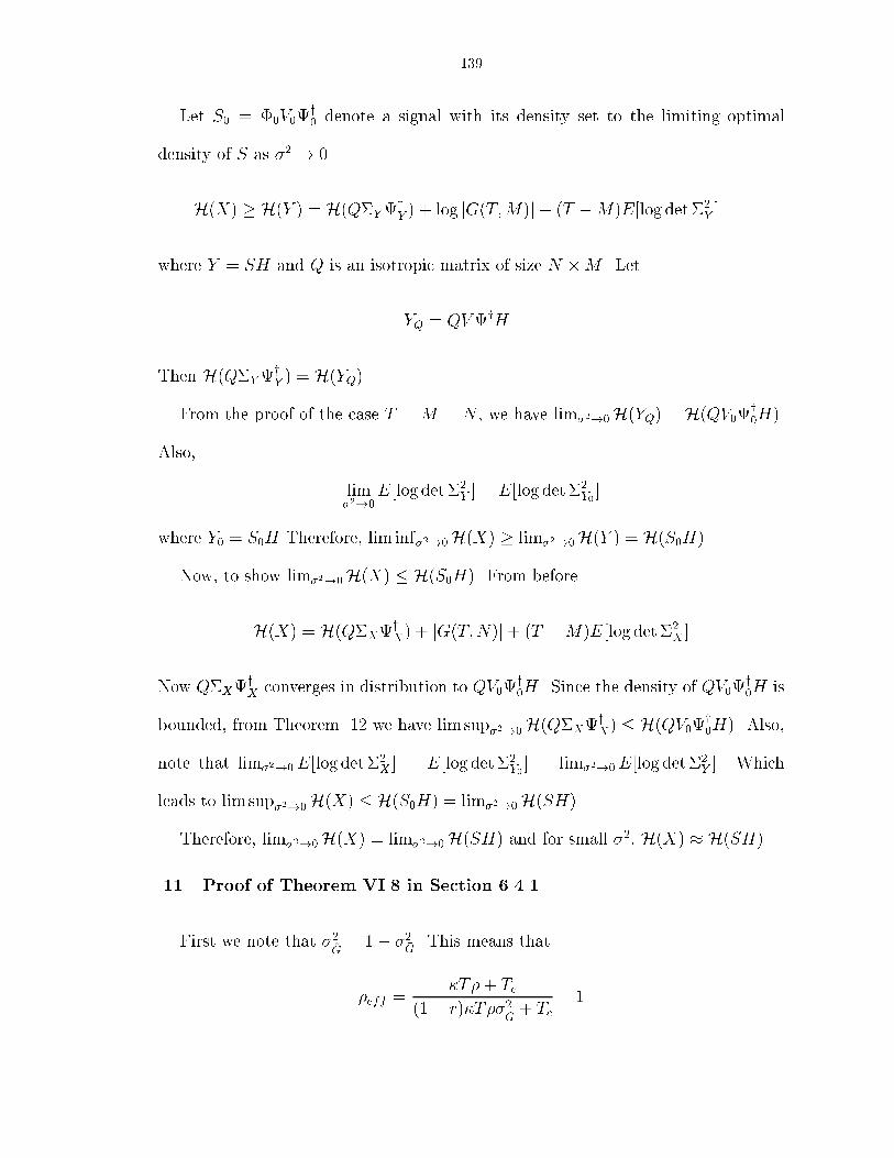
139Let S0 = �0V0y0 denote a signal with its density set to the limiting optimaldensity of S as �2 ! 0.H(X) � H(Y ) = H(Q�YyY ) + log jG(T;M)j+ (T �M)E[log det �2Y ]where Y = SH and Q is an isotropic matrix of size N �M . LetYQ = QVyHThen H(Q�YyY ) = H(YQ).From the proof of the case T = M = N , we have lim�2!0H(YQ) = H(QV0y0H).Also, lim�2!0E[log det �2Y ] = E[log det �2Y0 ]where Y0 = S0H Therefore, lim inf�2!0H(X) � lim�2!0H(Y ) = H(S0H).Now, to show lim�2!0H(X) � H(S0H). From beforeH(X) = H(Q�XyX) + jG(T;N)j+ (T �M)E[log det �2X ]Now Q�XyX converges in distribution to QV0y0H. Since the density of QV0y0H isbounded, from Theorem .12 we have limsup�2!0H(Q�XyX) � H(QV0y0H). Also,note that lim�2!0E[log det �2X ] = E[log det �2Y0 ] = lim�2!0E[log det �2Y ]. Whichleads to limsup�2!0H(X) � H(S0H) = lim�2!0H(SH).Therefore, lim�2!0H(X) = lim�2!0H(SH) and for small �2, H(X) � H(SH)..11 Proof of Theorem VI.8 in Section 6.4.1First we note that �2G = 1� �2�G. This means that�eff = �T�+ Tc(1� r)�T��2�G + Tc � 1

140Therefore, to maximize �eff we just need to minimize �2�G. Now,�2�G = 1NM trfE[ ~�G~�Gy]gwhere E[ ~�G~�Gy] = (IM + (1� r) �M SytSt)�1 INwhere � = M�2 . Therefore, the problem is the followingminSt:trfSytStg�(1��)TM 1M trf�IM + (1� r) �M SytSt��1gThis problem can be restated asmin�1;::: ;�M :P�m�(1��)TM 1M MXm=1 11 + (1� r) �M�mwhere �m, m = 1; : : : ;M are the eigenvalues of SytSt. The solution to the aboveproblem is �1 = : : : = �M = (1 � �)T . Therefore, the optimum St satis�es SytSt =(1� �)TIM . Which is the same as the optimum signal as derived in [33].This gives �2�G = 11+(1�r) �M (1��)T . Also, for this choice of St we obtain the elementsof G to be zero mean independent with Gaussian distribution. This gives�eff = �T�[Mr + �(1� �)T ]Tc(M + �(1� �)T ) + (1� r)�T�M.12 Proof of Theorem VI.9 in Section 6.4.1Now �eff = �T�[Mr + �(1� �)T ]Tc(M + �(1� �)T ) + (1� r)�T�M= T�Tc � (1� r)M (1� �)�+ � rMT�MTc+T�TcT�[Tc�(1�r)M ] � � Tc 6= (1� r)M= T 2�2Tc(M + T�) [(1� �)�+ �rMT� ] Tc = (1� r)M

141Consider the following three cases for the maximization of �eff over 0 � � � 1.Case 1. Tc = (1� r)M :We need to maximize (1 � �)� + � rMT� over 0 � � < 1. The maximum occurs at� = minf12 + rM2T� ; 1g which states that for su�cient small � no training is required.This result agrees with the result in Section 6.3.3 where the rician fading channelbasically behaves like an AWGN channel. In this caseT 2�2(1� r)M(M + T�)[�rMT� + �(1� �)]with � = minf12 + rM2T� ; 1g.Case 2. Tc > (1� r)M :In this case, �eff = T�Tc � (1� r)M (1� �)� + �� � �where � = rMT� and = MTc+T�TcT�[Tc�(1�r)M ] > 1. We need to maximize (1��)�+�� �� over0 � � � 1 which occurs at � = �p 2 � � � . Therefore,�eff = T�Tc � (1� r)M (p �p � 1� �)2When � = 1 we obtain Tc = T . Substituting � = 1 in the expression for �eff�eff = �T�[Mr + �(1� �)T ]Tc(M + �(1� �)T ) + (1� r)�T�Mwe obtain �eff = rT�T+(1�r)T� .Case 3. Tc < (1� r)M :In this case, �eff = T�(1� r)M � Tc (1� �)� + ���� where = MTc+T�TcT�[Tc�(1�r)M ] < 0. Maximizing (1��)�+�� �� over 0 � � � 1 we obtain� = +p 2 � � �. Therefore,�eff = T�Tc � (1� r)M (p� �p� + 1 + �)2

142Similar to the case Tc < (1�r)M when � = 1 we obtain Tc = T and �eff = rT�T+(1�r)T� ..13 Proof of Theorem VI.10 in Section 6.4.1Note that optimization over Tc makes sense only when � < 1. First, we examinethe case Tc > (1� r)M . The other two cases are similar. Let Q = minfM;Ng andlet �i denote the ith, i = 1; : : : ; Q non-zero eigenvalue of H1Hy1M . Then we haveCt � QXi=1 TcT E log(1 + �eff�i)Let Cl denote the lower bound on the RHS in the expression above. The idea is tomaximize Cl as a function of Tc. We havedCldTc = QXi=1 � 1T E log(1 + �eff�i) + TcT d�effdTc E � �i1 + �eff�i��Now, �eff for Tc > (1� r)M is given by�eff = T�Tc � (1� r)M (p �p � 1� �)2where = MTc+T�TcT�[Tc�(1�r)M ] and � = rMT� . It can be easily veri�ed thatd�effdTc = T�(p �p � 1� �)2[Tc � (1� r)M ]2 "s(1� r)M(M + T�)Tc(Tc + T�+ rM) � 1#Therefore,dCldTc = 1T QXi=1 E "log(1 + �eff�i)� �eff�i1 + �eff�i TcTc � (1� r)M "1�s(1� r)M(M + T�)Tc(Tc + T�+ rM) ##Since, TcTc�(1�r)M h1�q (1�r)M(M+T�)Tc(Tc+T�+rM) i < 1 and log(1 + x) � x=(1 + x) � 0 for allx � 0 we have dCldTc > 0. Therefore, we need to increase Tc as much as possible tomaximize Cl.

BIBLIOGRAPHY

143

144BIBLIOGRAPHY

[1] N. S. A. F. Naguib and A. R. Calderbank, \Space-time coding and signal processing for highdata rate wireless communications," IEEE Signal Processing Magazine, pp. 77{92, May 2000.[2] S. T. A-J van der Veen and A. Paulraj, \Blind estimation of multiple digital signals transmittedover �r channels," Signal Processing Letters, vol. 2, no. 5, pp. 99{102, May 1995.[3] M. D. T. A. Narula and G. W. Wornell, \Performance limits of coded diversity methods fortransmitter antenna arrays," IEEE Trans. on Inform. Theory, vol. 45, no. 7, pp. 2418{2433,Nov. 1999.[4] I. Abou-Faycal and B. Hochwald, \Coding requirements for multiple-antenna channels withunknown rayleigh fading," Bell Labs Technical Memorandum, Mar. 1999.[5] T. Aboulnasr and K. Mayyas, \Selective coe�cient update of gradient-based adaptive algo-rithms," Signal Processing, vol. 47, no. 5, pp. 1421{1424, May 1999.[6] T. S. Alexander, Adaptive Signal Processing: Theory and Applications, Springer-Verlag, NewYork, 1986.[7] I. C. ar and J. anos K}orner, Information Theory: Coding Theorems For Discrete MemorylessSystems, New York, NY: Academic Press, 1981.[8] S. L. Ariyavisitakul, \Turbo space-time processing to improve wireless channel capacity," IEEECommunications Magazine, vol. 48, no. 8, pp. 1347{1359, Aug. 2000.[9] T. J. R. B. M. Hochwald, T. L. Marzetta and W. Sweldens, \Systematic design of unitaryspace-time constellations," IEEE Trans. on Inform. Theory, vol. 46, no. 6, pp. 1962{1973,Sep. 2000.[10] T. M. Cover and J. A. Thomas, Elements of Information Theory, Wiley Series in Telecommu-nications, 1995.[11] C. C. A. H. D. Messerschmitt, D. Hedberg and P. Winship, \Digital voice echo canceller witha tms32020," Application report: SPRA129, Texas Instruments.[12] S. C. Douglas, \Analysis and implementation of the max-nlms adaptive �lter," Proceedings ofASIMOLAR-29, vol. 1, pp. 659l{663, 1996.[13] S. C. Douglas, \A family of normalized lms algorithms," IEEE Signal Processing Letters, vol.1, no. 3, pp. 49{51, March 1994.[14] S. C. Douglas, \Adaptive �lters employing partial updates," IEEE Trans. Acoust., Speech, andSig. Proc., vol. ASSP-44, pp. 209{216, March 1997.[15] P. F. Driessen and G. J. Foschini, \On the capacity formula for multiple input-multiple outputwireless channels: A geometric interpretation," IEEE Trans. on Communications, vol. 47, no.2, pp. 173{176, February 1999.

145[16] J. P. E. Biglieri and S. S. (Shitz), \Fading channels: Information-theoretic and communicationsaspects," IEEE Trans. on Inform. Theory, vol. 44, no. 6, pp. 2619{2692, Oct. 1998.[17] A. Y. E. Gautheir and J.-Y. Chouinard, \Capacity of multiple antenna systems in rayleighfading channels," Canadian Conference on Electrical and Computer Engineering, vol. 1, pp.275{279, 2000.[18] R. B. Ertel and P. Cardieri, \Overview of spatial channel models for antenna array communi-cation systems," IEEE Personal Communications, pp. 10{22, Feb. 1998.[19] A. L. F. R. Farrokhi, G. J. Foschini and R. A. Valenzuela, \Link-optimal space-time processingwith multiple transmit and receive antennas," To appear in IEEE Communication Letters.[20] A. Feuer and E. Weinstein, \Convergence analysis of lms �lter with uncorrelated gaussiandata," IEEE Trans. Acoust., Speech, and Sig. Proc., vol. ASSP-33, no. 1, pp. 222{229, Feb.1985.[21] G. J. Foschini, \Layered space-time architecture for wireless communication in a fading envi-ronment when using multiple antennas," Bell Labs Technical Journal, vol. 1, no. 2, pp. 41{59,1996.[22] G. J. Foschini and M. J. Gans, \On limits of wireless communications in a fading environmentwhen using multiple antennas," Wireless Personal Communications, vol. 6, no. 3, pp. 311{335,March 1998.[23] B. Friedlander and A. J. Weiss, \E�ects of model errors on signal reconstruction using a sensorarray," Proc. IEEE Int. Conf. Acoust., Speech, and Sig. Proc., vol. 4, pp. 552{555, 1993.[24] P. D. T. G. Caire and E. Biglieri, \Capacity of multi-antenna block fading channels," Com-munication Theory mini Conference, pp. 11{15, 1999.[25] E. B. G. Tarrico and G. Caire, \Limiting performance of block-fading channels with multipleantennas," Proc. of the IEEE Information Theory and Communications Workshop, pp. 27{29,1999.[26] A. Ganesan and A. M. Sayeed, \Bandwidth-e�cient exploitation of the degrees of freedom ina multipath fading channel," Proc. of IEEE Symposium on Information Theory, p. 161, June2000.[27] L. C. Godara, \Applications of antenna arrays to mobile communications, part ii: Beam-forming and direction-of-arrival considerations," IEEE Proceedings, vol. 85, no. 8, pp. 1195{1245, August 1997.[28] L. C. Godara, \Applications of antenna arrays to mobile communications, part i: Performanceimprovement, feasibility, and system considerations," IEEE Proceedings, vol. 85, no. 7, pp.1031{1060, July 1997.[29] M. Godavarti, \Implementation of a g.165 line echo canceller on texas instruments' tms320c3xand tms320c54x chips," ICSPAT Conference Proceedings, pp. 65{69, Sep. 1997.[30] A. Gorokhov, \Transmit diversity versus sdma: Analytic and numerical comparisons," Proc.of the IEEE Internation Conference on Communications, vol. 2, pp. 1020{1024, 2000.[31] A. Gorokhov, \Capacity of multiple-antenna rayleigh channel with a limited transmit diver-sity," Proc. of IEEE Symposium on Information Theory, p. 411, June 2000.[32] L. Guo, \Stability of recursive stochastic tracking algorithms," SIAM Journal on Control andOptimization, vol. 32, pp. 1195{1225, 1994.

146[33] B. Hassibi and B. M. Hochwald, \How much training is needed in multiple-antenna wirelesslinks?," Bell Labs Technical Memorandum, 2000.[34] A. O. Hero and T. L. Marzetta, \On computational cut-o� rate for space-time coding," Sub-mitted to IEEE Transactions on Information Theory.[35] B. M. Hochwald and T. L. Marzetta, \Unitary space-time modulation for multiple-antennacommunications in rayleigh at fading," IEEE Trans. on Inform. Theory, vol. 46, no. 2, pp.543{564, March 2000.[36] R. A. Horn and C. R. Johnson, Matrix Analysis, Cambridge University Press, 1996.[37] L. L. Horowitz and K. D. Senne, \Performance advantage of complex lms for controlling narrow-band adaptive arrays," IEEE Trans. Acoust., Speech, and Sig. Proc., vol. ASSP-29, no. 3, pp.722{736, June 1981.[38] B. L. Hughes, \Di�erential space-time modulation," Submitted to IEEE Transactions on In-formation Theory, Feb. 2000.[39] B. L. Hughes, \Optimal space-time constellations from groups," Submitted to IEEE Transac-tions on Information Theory, March 2000.[40] M. D. T. I. C. Abou-Faycal and S. S. (Shitz), \The capacity of discrete-time memorylessrayleigh fading channels," To Appear in IEEE Transactions on Information Theory.[41] D. D. F. J. Cui and A. U. H. Sheikh, \Performance evaluation of optimum combining inthe presence of co-channel interference and channel correlation for wireless communicationsystems," Mobile Networks and Applications, vol. 2, no. 4, pp. 315{324, Jan 1998.[42] J. S. J. H. Winters and R. D. Gitlin, \The impact of antenna diversity on the capacity ofwireless communication systems," IEEE Trans. on Communications, vol. 42, pp. 1740{1751,1994.[43] S. D. J. Yang and A. Swindlehurst, \Improved signal copy with partially known or unknownarray response," Proc. IEEE Int. Conf. Acoust., Speech, and Sig. Proc., vol. 4, pp. 265{268,1994.[44] A. R. Kuruc, \Lower bounds on multiple-source direction �nding in the presence of direction-dependent antenna-array-calibration errors," Technical Report 799, MIT Lincoln Laboratory,Oct. 1989.[45] L. L. L. Guo and G. J. Wang, \Necessary and su�cient conditions for stability of lms," IEEETrans. Automatic Control, vol. 42, no. 6, , 1997.[46] B. G. H. M. J. Gingell and L. D. Humphrey, \A block mode update echo canceller using customlsi," GLOBECOM Conference Record, vol. 3, pp. 1394{1397, Nov. 1983.[47] P. P. M. M. R. Andrews and R. deCarvalho, \Tripling the capacity of wireless communicationsusing electromagnetic polarization," Nature, vol. 409, pp. 316{318, Jan. 2001.[48] T. L. Marzetta and B. M. Hochwald, \Capacity of a mobile multiple-antenna communicationlink in rayleigh at fading channel," IEEE Trans. on Inform. Theory, vol. 45, no. 1, pp. 139{157, Jan 1999.[49] A. S. N. Benvenuto, P. Bisaglia and L. Tomba, \Worst case equalizer for noncoherent hiperlanreceivers," IEEE Trans. on Communications, vol. 48, no. 1, pp. 28{36, January 2000.[50] H.-J. S. N. Sharma and E. Geraniotis, \A novel approach for multi-antenna systems," Proc. ofthe IEEE Internation Conference on Communications, vol. 3, pp. 1264{1269, 2000.

147[51] A. Narula, \Information theoretic analysis of multiple-antenna transmission diversity," Ph.D.Dissertation, MIT, Cambridge, MA, 1997.[52] K. M. W. P. Stoica, M. Viberg and Q. Wu, \Maximum-likelihood bearing estimation withpartly calibrated arrays in spatially correlated noise �elds," IEEE Trans. on Signal Processing,vol. 44, no. 4, pp. 888{899, Apr. 1996.[53] M. V. P. Stoica, B. Ottersten and R. L. Moses, \Maximum likelihood array processing forstochastic coherent sources," IEEE Trans. on Signal Processing, vol. 44, no. 1, pp. 96{105,Jan. 1996.[54] D. N. C. T. P. Viswanath and V. Ananthram, \Asymptotically optimal water�lling in multipleantenna multiple access channels," Proc. of IEEE Symposium on Information Theory, p. 466,June 2000.[55] E. M. R. Aguech and P. Priouret, \On a perturbation approach for the analysis of stochastictracking algorithms," To appear in SIAM Journal on Control and Optimization.[56] S. Rice, \Mathematical analysis of random noise," Bell Systems Technical Journal, vol. 23, ,1944.[57] M. V. S. Talwar and A. Paulraj, \Blind estimation of multiple co-channel digital signals usingan antenna array," Signal Processing Letters, vol. 1, no. 2, pp. 29{31, Feb. 1994.[58] M. V. S. Talwar and A. Paulraj, \Blind separation of synchronous co-channel digital signalsusing an antenna array { part i: Algorithms," IEEE Trans. on Signal Processing, vol. 44, no.5, pp. 1184{1197, May 1996.[59] A. M. Sengupta and P. P. Mitra, \Capacity of multivariate channels with multiplicative noise:I-randommatrix techniques and large-n expansions for full transfer matrices," Bell LaboratoriesTechnical Report.[60] N. Seshadri and J. H. Winters, \Two signaling schemes for improving the error performanceof frequency division duplex (fdd) transmission systems using transmitter antenna diversity,"Proc. of the IEEE Vehicular Technology Conference, pp. 508{511, 1993.[61] V. Solo and X. Kong, Adaptive Signal Processing Algorithms, Prentice-Hall, Englewood Cli�s,NJ, 1995.[62] A. Swindlehurst, \Maximum a posteriori approach to beamforming in the presence of cali-bration errors," Proc. of the IEEE Workshop on Statistical Signal and Array Processing, pp.82{85, 1996.[63] A. Swindlehurst, \Detection and estimation in the presence of signals with uncalibrated spatialstructure," Signal Processing, vol. 50, pp. 29{37, Apr. 1996.[64] I. E. Telatar, \Capacity of multi-antenna gaussian channels," European Transactions onTelecommunications, 199.[65] N. S. V. Tarokh and A. R. Calderbank, \Space-time codes for high data rate wireless com-munication: Performance criterion and code construction," IEEE Trans. on Communications,vol. 44, no. 2, pp. 744{765, March 1998.[66] N. S. V. Tarokh, A. Naguib and A. R. Calderbank, \Space-time codes for high data ratewireless communication: Performance criteria in the presence of channel estimation errors,mobility, and multiple paths," IEEE Trans. on Inform. Theory, vol. 47, no. 2, pp. 199{207,Feb. 1999.[67] S. Verd�u, \On channel capacity per unit cost," IEEE Trans. on Inform. Theory, vol. 36, no.5, pp. 1019{1030, September 1990.

148[68] V. Weerackody, \Diversity of the direct-sequence spread spectrum system using multiple trans-mit antennas," Proc. of the IEEE Internation Conference on Communications, pp. 1775{1779,1993.[69] J. H. Winters, \Optimum combining in digital mobile radio with co-channel interference,"IEEE Journal of Selected Areas in Communication, vol. 2, pp. 528{539, 1984.[70] J. H. Winters, \Optimum combining for indoor radio systems with multiple users," IEEETrans. on Communications, vol. 35, pp. 1222{1230, 1987.[71] J. H. Winters and J. Salz, \Upper bounds on the bit error rate of optimum combining inwireless systems," Proc. of the IEEE Vehicular Technology Conference, vol. 2, pp. 942{946,1994.[72] A. Wittenben, \Basestation modulation diversity for digital simulcast," Proc. of the IEEEVehicular Technology Conference, pp. 848{853, 1991.[73] J. Yang and A. L. Swindlehurst, \The e�ects of array calibration errors on df-based signal copyperformance," IEEE Trans. on Signal Processing, vol. 43, no. 11, pp. 2724{2732, Nov. 1995.[74] L. Zheng and D. N. C. Tse, \Packing spheres in the grassmann manifold: A geometric approachto the non-coherent multi-antenna channel,".

ABSTRACTAntenna Arrays in Wireless CommunicationsbyMahesh GodavartiChair: Alfred O. Hero-III

Multiple-antenna wireless systems have been gaining in popularity due to demandfor higher data rates and the limited bandwidth available for communication. Mul-tiple antennas have been used both at the transmitter and the receiver traditionallyin a beamformer (array processing). However, it was shown recently that in thepresence of fading the optimal solution in terms of capacity (upper limit on datarates with arbitrarily small error probabilities) involves other structures that are notbeamformers.We investigate both aspects of multiple-antenna wireless communication systemsin this thesis. We investigate variants of the popular adaptive LMS algorithm knownas the Partial Update LMS Algorithms for the purposes of beamforming in a wirelesscommunication scenario. Partial update LMS algorithms involve partial updatingof the �lter coe�cients as opposed to the full update in a regular LMS algorithm.For example, the coe�cients can be divided into even and odd coe�cient sets and

1the sets could be updated alternatively. We investigate the existing partial updatealgorithms and also a propose a new variant which exhibits none of the disadvantagesof the existing algorithms.The second aspect of the multiple-antenna wireless communcation systems is theshannon capacity. Existing work so far has concentrated on deriving capacity ex-pressions for the case of rayleigh fading channels. In this thesis, we investigate themaximum possible data rate a�ordable by communication systems in the presenceof rician fading. We derive capacity expressions, capacity achieving signal structuresas well as upper and lower bounds on capacity for two new models (proposed fortractable analysis) for rician fading. We also derive asymptotic capacity expressions,capacity achieving signal structures and upper and lower bounds on capacity for thestandard rician fading channel model.