Antarctic climate, Southern Ocean circulation patterns ... · greenhouse climate of the Eocene. 1. Introduction The Paleogene time period (66 to 23 Ma) encompasses the transition

Open Research OnlineThe Open University’s repository of research publicationsand other research outputs

Antarctic climate, Southern Ocean circulation patterns,and deep water formation during the EoceneJournal ItemHow to cite:

Huck, Claire E.; van de Flierdt, Tina; Bohaty, Steven M. and Hammond, Samantha J. (2017). Antarcticclimate, Southern Ocean circulation patterns, and deep water formation during the Eocene. Paleoceanography, 32(7)pp. 674–691.

For guidance on citations see FAQs.

c© 2017 American Geophysical Union

Version: Version of Record

Link(s) to article on publisher’s website:http://dx.doi.org/doi:10.1002/2017PA003135

Copyright and Moral Rights for the articles on this site are retained by the individual authors and/or other copyrightowners. For more information on Open Research Online’s data policy on reuse of materials please consult the policiespage.

oro.open.ac.uk

Antarctic climate, Southern Ocean circulation patterns,and deep water formation during the EoceneClaire E. Huck1,2 , Tina van de Flierdt1, Steven M. Bohaty2 , and Samantha J. Hammond3

1Department of Earth Science and Engineering, Imperial College London, London, UK, 2Ocean and Earth Science, NationalOceanography Centre Southampton, University of Southampton, Southampton, UK, 3Environment, Earth and EcosystemsDepartment, Open University, Milton Keynes, UK

Abstract We assess early-to-middle Eocene seawater neodymium (Nd) isotope records from sevenSouthern Ocean deep-sea drill sites to evaluate the role of Southern Ocean circulation in long-termCenozoic climate change. Our study sites are strategically located on either side of the Tasman Gateway andare positioned at a range of shallow (<500 m) to intermediate/deep (~1000–2500 m) paleowater depths.Unradiogenic seawater Nd isotopic compositions, reconstructed from fish teeth at intermediate/deepIndian Ocean pelagic sites (Ocean Drilling Program (ODP) Sites 738 and 757 and Deep Sea Drilling Project(DSDP) Site 264), indicate a dominant Southern Ocean-sourced contribution to regional deep waters(εNd(t) = �9.3 ± 1.5). IODP Site U1356 off the coast of Adélie Land, a locus of modern-day Antarctic BottomWater production, is identified as a site of persistent deep water formation from the early Eocene to theOligocene. East of the Tasman Gateway an additional local source of intermediate/deep water formation isinferred at ODP Site 277 in the SW Pacific Ocean (εNd(t) = �8.7 ± 1.5). Antarctic-proximal shelf sites (ODP Site1171 and Site U1356) reveal a pronounced erosional event between 49 and 48 Ma, manifested by ~2 εNd unitnegative excursions in seawater chemistry toward the composition of bulk sediments at these sites. Thiserosional event coincides with the termination of peak global warmth following the Early Eocene ClimaticOptimum and is associated with documented cooling across the study region and increased export ofAntarctic deep waters, highlighting the complexity and importance of Southern Ocean circulation in thegreenhouse climate of the Eocene.

1. Introduction

The Paleogene time period (66 to 23 Ma) encompasses the transition from the warm “greenhouse” climatestate of the late Paleocene and early Eocene (59 to 48 Ma) to the colder “icehouse” climate state of theOligocene (34 to 23 Ma) [Zachos et al., 2008]. The warmest climatic conditions of the Paleogene occurredduring the Early Eocene Climatic Optimum (EECO) (~52 to 48 Ma) [Sexton et al., 2011; Zachos et al., 2008]when deep ocean temperatures reached ~12°C [Littler et al., 2014; Zachos et al., 2001] and polar regions werecharacterized by extreme warmth with Antarctic coastal summer temperatures in excess of 20°C [Pross et al.,2012]. Following the EECO, global temperatures declined until the prevailing greenhouse conditions endedat the Eocene-Oligocene Transition (EOT) (~34 Ma) with continental-scale glaciation of Antarctica and oceancooling [e.g., Coxall et al., 2005; Dunkley Jones et al., 2008; Ehrmann et al., 1992; Houben et al., 2013; Lear et al.,2008; Liu et al., 2009; Passchier et al., 2017; Zachos et al., 2001].

The relative role of decreasing atmospheric CO2 versus changing Southern Ocean circulation patterns result-ing from the opening of high-latitude ocean gateways (i.e., Drake Passage and Tasman Gateway) in the tran-sition from greenhouse to icehouse climates during the Paleogene has been much debated [e.g., DeContoand Pollard, 2003; Galeotti et al., 2016; Goldner et al., 2014; Huber and Nof, 2006; Kennett, 1977; Sijp et al.,2011], with several studies highlighting the complex nature of the long-term cooling trend during theEocene [Bohaty and Zachos, 2003; Douglas et al., 2014; Scher et al., 2014]. Eocene reconstructions of CO2 con-centrations indicate a decline from ≥1400 ppm to ~500 ppm by the early Oligocene [Anagnostou et al., 2016;Galeotti et al., 2016; Pagani et al., 2005, 2011]. Although deep oceans cooled during the Eocene [e.g., Zachoset al., 2001], much less is known about the associated changes in circulation patterns and dominant sourceregions of deep water formation. Modeling and geochemical data-based studies have proposed both theSouthern Ocean and the low latitudes as regions of deep water formation during the warmest periods ofthe Cretaceous and early Cenozoic [e.g., Brass et al., 1982; Kennett and Stott, 1991; Bice et al., 1997; Crameret al., 2009; Hague et al., 2012; Pak and Miller, 1992; Scher and Martin, 2004; Sijp and England, 2016;

HUCK ET AL. EOCENE SOUTHERN OCEAN CIRCULATION 674

PUBLICATIONSPaleoceanography

RESEARCH ARTICLE10.1002/2017PA003135

Key Points:• Distinct neodymium water masssignature recorded in intermediate/deep waters in the SW Pacific duringthe Eocene

• Local deep water formation on AdélieCoast during Eocene greenhousewarmth

• A previously unidentified Antarcticerosional event occurred at 49-48 Ma

Supporting Information:• Supporting Information S1

Correspondence to:C. E. Huck,[email protected]

Citation:Huck, C. E., T. van de Flierdt,S. M. Bohaty, and S. J. Hammond (2017),Antarctic climate, Southern Oceancirculation patterns, and deep waterformation during the Eocene,Paleoceanography, 32, 674–691,doi:10.1002/2017PA003135.

Received 10 APR 2017Accepted 29 MAY 2017Accepted article online 11 JUN 2017Published online 3 JUL 2017

©2017. American Geophysical Union.All Rights Reserved.

Thomas, 2004; Thomas et al., 2014], leaving large uncertainty about the link between ocean circulation andclimate during the early Cenozoic greenhouse (e.g., the early Eocene “equable climate paradox”) [Huber andCaballero, 2011]. This is in part due to a lack of detailed records documenting Eocene climate and oceancirculation in key geographical areas.

In this study we reconstruct Southern Ocean water mass distributions during the early to middle Eocene fromseven different Integrated Ocean Drilling Program (IODP), Ocean Drilling Program (ODP), and Deep SeaDrilling Project (DSDP) sites in the Tasman region, Indian Ocean, and the Southwestern Pacific Ocean usingthe neodymium (Nd) isotopic composition of fossil fish teeth. Neodymium is incorporated into the teeth dur-ing the fossilization process at the sediment-water interface and records the composition of bottomwaters atthe time of deposition [Martin and Haley, 2000; Shaw andWasserburg, 1985]. The short residence time of Nd inseawater (~400 to 1000 years) [Arsouze et al., 2009; Tachikawa et al., 2003] allows the Nd isotope compositionof fish teeth to be used as a tracer of prevailing water masses and ocean circulation. Our new Southern Oceanrecords provide insights into (i) pathways of deep and intermediate water masses during the Eocene, (ii) loca-tions of local bottom water formation, and (iii) transient perturbations of seawater chemistry in the SouthernOcean due to changes in Antarctic climate and erosion. We suggest that the Southern Ocean acted as a majorsource of deep water to the surrounding ocean basins during the Eocene, highlighting the importance of thisregion in controlling climate even during the warmest periods of the Cenozoic.

2. Study Sites and Age Models

An overview of the study sites is presented in Table 1 and discussed in more detail below. Additional infor-mation including details of the age models used can be found in the supporting information.

2.1. Pelagic Sites

Four pelagic Southern Ocean drill sites were sampled to obtain low-resolution records of intermediate/deepwater masses in the ocean basins adjacent to the Eocene Tasman Gateway region (Figure 1). Three of thesesites are located in the Indian Ocean: Deep-Sea Drilling Project (DSDP) Site 264 (34°580S, 112°020E) [Hayeset al., 1975], and Ocean Drilling Program (ODP) Sites 738 (62°420S, 82°470E) [Barron et al., 1989] and 757(17°010S, 88°100E) [Peirce et al., 1989]. One additional site, DSDP Site 277 (52°130S, 166°110E) [Kennett et al.,1975], is located in the SW Pacific. The sediments at these four pelagic sites consist predominantly of calcar-eous nannofossil ooze, and Eocene paleowater depths range from 1000 to 1500 m for Sites 277, 738, and 757[Hollis et al., 1997; Roberts et al., 2011; Zachos et al., 1992] to 2500 m for Site 264 (see supporting information).Site 738 has approximately remained at its present latitude (62°S) since the Eocene. Sites 264, 277, and 757were located farther south than their current latitudes, at ~50°S, ~65°S, and ~40°S, respectively [Hollis et al.,2015; van Hinsbergen et al., 2015; Zachos et al., 1992]. Age models for these sites are predominantly basedon biostratigraphy with ages updated to the GTS2012 age scale [Bohaty et al., 2009; Huber and Quillévéré,2005; Vandenberghe et al., 2012].

2.2. Shelf Sites

Three shelf sites located on both the Indian (IODP Site U1356) and Pacific (ODP Sites 1171 and 1172) sides ofthe Tasman Gateway (Figure 1) were included in this study. We use the age models of Bijl et al. [2013a] for allthree of these sites, which are based on magnetostratigraphy and nannofossil and dinocyst biostratigraphycalibrated to the GTS2012 timescale.

Table 1. Summary of Site and Sample Information Considered in This Studya

Leg Program Site Hole/s Cores Sample Range (mbsf) Present Location Water Depth (m) Paleolatitude Paleodepth (m)

28 DSDP 264 A 3R-4R 140.30–151.35 34°580S, 112°020E 2873 ~50°S ~250029 DSDP 277 - 38R-43R 389.20–435.00 52°130S, 166°110E 1232 ~65°S ~1000119 ODP 738 B, C 17X-24X, 6R-8R 140.95–264.70 62°420S, 82°470E 2253 ~62°S ~1500121 ODP 757 B 17H-21X 150.00–207.25 17°010S, 88°100E 1652 ~40°S ~1000–1500189 ODP 1171 D 35R-71R 565.52–912.85 48°290S, 149°60E 2150 ~70°S 500–1000189 ODP 1172 D 8R-14R 536.36–597.60 43°570S, 149°550E 2620 ~65°S 500–1000318 IODP U1356 A 67R-106R 633.47–998.73 63°180S, 135°590E 4003 ~65°S 500–1000

aSee main text for references.

Paleoceanography 10.1002/2017PA003135

HUCK ET AL. EOCENE SOUTHERN OCEAN CIRCULATION 675

ODP Site 1171 (48°290S, 149°60E) on the South Tasman Rise (STR) was positioned adjacent to the Antarcticmargin at ~70°S during the Eocene [Bijl et al., 2013b; Cande and Stock, 2004]. ODP Site 1172 (43°570S,149°550E) was positioned on the East Tasman Plateau (ETP) and was also located farther south at ~65°S duringthe Eocene [Bijl et al., 2013b; Exon et al., 2001]. Both sites subsided through the Eocene, with the depositionalenvironments evolving from restricted shallow-shelf (<500 m paleodepth) to more hemipelagic (~1000 mpaleodepth) conditions by the late Eocene [Exon et al., 2001; Scher et al., 2015].

Site U1356 (63°180S, 135°590E)was positionedwithin the enclosedAustral-Antarctic Gulf (AAG; Figure 1) duringtheearly andmiddle Eocene. Progressive subsidenceof the siteoccurred through theEoceneandOligocene, asevidencedby lithological anddinocyst assemblagechanges [Bijl etal., 2013a,2013b;Escutia etal., 2011]. Existingpaleodepth reconstructions suggestdeepening fromashallowmarine setting (~500mpaleodepth) in theearlyEocene to amorehemipelagic slope setting (>1000m)by the earliestOligocene; however, there is a significantlevel of uncertainty associated with these estimates [Escutia et al., 2011]. The stratigraphic sequence of SiteU1356 is interrupted by two hiatuses which span from ~51 to 49 Ma and from ~46 to 33.6 Ma [see Bijl et al.,2013b;Houbenetal., 2013;Tauxeetal., 2012]. For thepurposesofour study, the threehiatus-boundsedimentarypackages recovered at Site U1356 will be designated according to age and referenced to as follows: the earlyEocene (1006.4 to 948.8 meters below seafloor (mbsf); ~54 to 51.5 Ma), “mid”-Eocene (948.8 to 894.68 mbsf;~49 to 46 Ma), and Oligocene (894.68 to 633.47 mbsf; ~33.5 to 25 Ma).

3. Methods3.1. Neodymium Isotopes3.1.1. Fossil Fish Tooth Sample PreparationA total of 41 samples across all study sites were prepared for fish tooth Nd isotope analyses for this study. Wealso include data from an additional 25 fish tooth samples analyzed frommid-Eocene Core U1356A-98R [Hucket al., 2016]. Fossil fish teeth were picked from the >63 μm sediment fractions that were prepared by wetsieving. To test whether a full oxidative-reductive cleaning protocol was necessary for fish tooth analysis,two samples each from Site U1356, Site 1171, and Site 1172, reflecting a range of ages, different sedimentcompositions, and paleowater depths, were split into two aliquots. One sample split (referred to as “cleaned”)was subjected to a full oxidative-reductive cleaning protocol to remove Fe-Mn oxyhydroxide coatings usingthe method adapted from Boyle and Keigwin [1985]. The other split (“uncleaned”) was treated with the sim-plified MQ-water and methanol-only cleaning method of Martin and Haley [2000] (supporting informationTable S1). Cleaned fish tooth samples were subsequently dissolved overnight in 2 M HCl. A fossil bone

Figure 1. (a) Location of IODP/ODP/DSDP drill sites considered in this study illustrated on a 45 Ma paleogeographic recon-struction made using Ocean Drilling Stratigraphic Network online toolkit (www.odsn.de). Circles denote pelagic sites(≥1000 m), and squares denote shallow shelf sites (<500 m). Major Southern Ocean gateways are outlined with dashedlines. White outlined areas represent submerged plateaus: KP = Kerguelen Plateau, NER = Ninetyeast Ridge,NP = Naturaliste Plateau, CP = Campbell Plateau, and LHR = Lord Howe Rise. (b) Early Eocene reconstruction of shelf sites inthe AAG adapted from Bijl et al. [2013a].

Paleoceanography 10.1002/2017PA003135

HUCK ET AL. EOCENE SOUTHERN OCEAN CIRCULATION 676

composite standard was used for quality control and was digested following the method described inChavagnac et al. [2007]. In short, the fish tooth and bone standard was digested by dissolving 50 mg of mate-rial in 3 M HNO3 in a sealed Teflon beaker on a hotplate at 130°C. Any residue remaining after this step wassubjected to a further 48 h digestion in a 3:1mixture of 15MHNO3 and 27MHF. Neodymium from all sampleswas then collected using a standard two-stage ion exchange chromatography to first separate the rare earthelements (REEs) from the sample matrix using TRU-Spec resin (100–120 μm bead size) and to then isolate Ndfrom the other REEs using Ln-Spec resin (50–100 μm bead size) (modified after Pin and Zalduegui [1997]).3.1.2. Bulk Sediment Sample PreparationBulk sediment Nd isotopic composition was determined for 12 samples from Site U1356 and four samplesfrom Site 1171. A further six bulk sediment samples from mid-Eocene core U1356A-98R from Huck et al.[2016] are also included in the sample set. For these analyses, 0.5–1.0 g of sediment was oven dried, comple-tely homogenized using a mortar and pestle, and ~100 mg of the powdered sample was weighed anddigested using a mixture of 0.5 mL 20 M HClO4, 1 mL 15 M HNO3, and 3 mL 27 M HF. Fe-Mn coatings werenot removed from the sediment samples in our study, as previous work on Eocene-aged samples at SiteU1356 has shown the contributions from authigenic phases to the final Nd isotopic composition to be neg-ligible (i.e., <1% total signal) [Huck et al., 2016]. The bulk samples were processed using the same columnchemistry used for the fish teeth.3.1.3. Neodymium Isotope MeasurementsNeodymium isotope ratios for fish tooth and sediment samples were determined at Imperial College Londonon a Nu Plasma multi-collector inductively coupled plasma mass spectrometer operated in static mode(supporting information Table S1). We used a 146Nd/144Nd ratio of 0.7219 to correct for instrumental massbias. Samarium (Sm) interference can be adequately corrected if the 144Sm signal contributes less than0.1% of the 144Nd signal. The Sm contribution in all our samples was well below this level. Replicate analysesof the Nd standard JNdi [Tanaka et al., 2000] yielded 143Nd/144Nd ratios from 0.511937 ± 0.000015 to0.512251 ± 0.000015 (2σ, n = 316) depending on daily running conditions over 29 months. External reprodu-cibility of sediment samples was monitored using USGS rock standards BCR-1 and BCR-2, which yielded ratiosfrom 0.512651 ± 0.000014 to 0.512655 ± 0.000022 and from 0.512632 ± 0.000016 to 0.512649 ± 0.000016,respectively. These values are indistinguishable from the ratios published by Weis et al. [2006] (BCR-1:0.512646 ± 0.000016; BCR-2: 0.512638 ± 0.000015). The fossil bone composite standard yielded a143Nd/144Nd ratio of 0.512377 ± 0.000014 (2σ, n = 8), which agrees within error with ratios published byChavagnac et al. [2007] and Scher and Delaney [2010]. Procedural blanks were consistently below 10 pg.

To correct for the decay of 147Sm to 144Nd within the fish teeth over time we used Sm and Nd concentrationsobtained from one or more samples at every site (supporting information Table S2). 147Sm/144Nd ratios for allsamples are between 0.124 and 0.174 and are consistent with values for Cretaceous to Miocene fossil fishtooth material [Martin and Scher, 2006; Moiroud et al., 2013; Thomas et al., 2003]. These maximum and mini-mum 147Sm/144Nd ratios would yield a difference of between 10 and 30 ppm if applied to εNd(t) calculationsfor the same samples, which is within the external reproducibility reported. We therefore applied a site-specific average value (147Sm/144Nd = 0.128 to 0.153) to all samples and denote all 147Sm decay-correctedNd isotope data as εNd(t) (where εNd is the deviation of the 143Nd/144Nd ratio measured in a sample from thatof the chondritic uniform reservoir in parts per 10,000 [Jacobsen and Wasserburg, 1980] and (t) denotes thesample correction for radiogenic ingrowth over time).

3.2. Rare Earth Elements

The full suite of REE concentrations were determined for 10 fossil fish tooth samples from the early Eoceneand Oligocene sections from Site U1356 and are compiled with a further 16 mid-Eocene samples fromHuck et al. [2016]. Two samples each from Sites 1171 and 1172 and one sample each from Sites 757, 738,264, and 277 were also analyzed. Major and trace element analysis was performed at the Open Universityusing an Agilent 7500s ICP-MS (supporting information Table S2). Oxide interferences were kept below0.3% for CeO+/Ce+ and 0.8% for (Ce++/Ce+). Analyses were standardized against seven synthetic referencematerials selected for their similarity to the samples that were measured at the beginning and end of eachanalytical run. Detection limits for elements with atomic masses greater than 85 were typically <10 ppt insolution but were somewhat higher for lighter elements (10–100 ppt in solution). Precision was routinely bet-ter than ±2% for elements heavier than rubidium (Rb) (where concentrations exceed 0.5 ppm) and 2–4% for

Paleoceanography 10.1002/2017PA003135

HUCK ET AL. EOCENE SOUTHERN OCEAN CIRCULATION 677

lighter elements. All sample REE data were normalized to Post Archean Shale (PAAS) concentrations [Taylorand McLennan, 1985]. The Ce anomaly for fish tooth samples (Ce/Ce*) was calculated following De Baaret al. [1985], where Ce/Ce* = 2Cen/(Lan + Prn).

4. Results4.1. Fossil Fish Tooth Nd Isotopic Compositions

εNd(t) values of fish tooth samples from all pelagic sites in this study yield an average value of�9.1 ± 1.6 (2sd,n = 19). Indian Ocean Sites 264, 738, and 757 range from�10.7 to�7.8 within the time interval between ~52and 44 Ma (average εNd(t) = 9.3 ± 1.5, 2sd, n = 13; supporting information Table S1 and Figure 2). The mostunradiogenic values at Sites 738 and 757 (εNd(t) = �10.7 and �9.8, respectively) occur between ~50 and48.5 Ma, with increasingly radiogenic compositions recorded at these sites between ~48 and 44 Ma. Thethree fish tooth samples from Site 264 have a similar isotopic composition (εNd(t) =�9.6 to�9.1). εNd(t) valuesof fish tooth samples from the pelagic SW Pacific Site 277 range from�9.7 to�7.3 between ~53 and ~47 Ma(average εNd(t) = �8.7 ± 1.7, 2sd, n = 6). The most negative εNd(t) value of �9.7 recorded at Site 277 occurs at~49 Ma (Figure 2).

εNd(t) values of early to middle Eocene-aged fish tooth samples at shelf Sites 1171 and 1172 span a range of�8.9 to �5.3. The most negative Nd isotopic composition recorded at Site 1172 occurs at ~50 Ma(εNd(t) =�7.9), whereas the fish tooth εNd(t) record at Site 1171 contains two negative excursions to minimumvalues of �8.9 at ~48.7 Ma and �8.2 at ~47.8 Ma (Figure 2). Including previously published data from Hucket al. [2016], compiled fish tooth εNd(t) values spanning the early Eocene to Oligocene (~54 to ~25 Ma) atIODP Site U1356 span a range of ~3 epsilon units (εNd(t) = �9.6 to �12.4) (Figure 2 and supporting informa-tion Table S1). Early Eocene fish teeth at Site U1356 have an average Nd isotope εNd(t) value of �10.7 ± 1.0(2sd, n = 11). During the mid-Eocene interval, a negative excursion to a minimum value of �12.4 is observedat 48.2 Ma. Within the Oligocene section of Site U1356, εNd(t) values vary by 1 epsilon unit between�10.2 and�11.2 with an average value of �10.7 ± 0.8 (2sd, n = 8), similar to the average early Eocene value.

4.2. Site U1356 and Site 1171 Bulk Sediment Nd Isotopic Compositions

At Site U1356, the Nd isotopic composition of bulk sediment samples from the early to mid-Eocene interval(~47 to 53 Ma) of this study and Huck et al. [2016] span a narrow range of ~1.7 epsilon units (�13.1 to�14.8)(Figure 3 and supporting information Table S1). These bulk sediment values are more negative than fish toothεNd(t) values by at least 2 epsilon units throughout the study section (Figure 3 and supporting informationTable S1) [Huck et al., 2016]. Across the early to middle Eocene (~49 and 47.5 Ma) interval of Site 1171, theNd isotopic composition of bulk sediment shows limited variability (εNd(t) = �9.3 to �9.8) in contrast to thelarge amplitude variations observed in fish tooth samples. Similar to the results obtained from Site U1356,the bulk sediment εNd(t) values at Site 1171 are lower than the value obtained from fish teeth from the sameinterval (Figure 3) by ~2 epsilon units.

4.3. Fossil Fish Tooth REE Patterns

The REE patterns of fossil fish tooth samples were primarily generated to confirm a seawater-derived signalfor Nd in all of our samples. Fish tooth samples from pelagic Sites 738, 757, 277, and 264 yielded middle-REEenriched patterns with a pronounced negative Ce anomaly (Ce/Ce* = 0.3 to 0.6) and a positive yttrium (Y)anomaly (Figure 4). Such patterns, as well as low overall REE concentrations, are diagnostic of a seawater ori-gin [e.g., German and Elderfield, 1990; Scher et al., 2011]. The fish tooth REE patterns from shelf Sites 1171,1172, and U1356 show a similar enrichment in mid-REEs but a positive Ce anomaly (Ce/Ce* = 1.0 to 1.9)(Figure 4). The positive Ce anomalies may arise from increased weathering of proximal continental regionsand/or remobilized REEs from authigenic or organic coatings [e.g., Elderfield and Pagett, 1986; Freslon et al.,2014; Huck et al., 2016;Wright et al., 1987]. Oligocene fish tooth REE concentrations at Site U1356 (gray colorin Figure 4 and supporting information Table S2) are generally more enriched than those of the Eocene sam-ples (dark and light green color in Figure 4 and supporting information Table S2). All cleaned and uncleanedfish tooth samples from pelagic and shelf sites show similar REE patterns, with cleaned samples having con-sistently lower REE concentrations (supporting information Table S2).

Paleoceanography 10.1002/2017PA003135

HUCK ET AL. EOCENE SOUTHERN OCEAN CIRCULATION 678

Figure 2. (a) Eocene-Oligocene Nd isotopic composition of fossil fish teeth and debris at Site U1356 from this study andHuck et al. [2016]. (b) Early to middle Eocene Nd isotope data for fossil fish tooth samples from shallow Sites 1171(orange squares) and 1172 (yellow squares) and U1356 (light green squares). (c) Pelagic Sites 757 (pink circles), 738 (purplecircles), 264 (red circles), and 277 (blue circles).

Paleoceanography 10.1002/2017PA003135

HUCK ET AL. EOCENE SOUTHERN OCEAN CIRCULATION 679

5. Discussion

To evaluate ocean circulation in the Southern Ocean during the Eocene, we separate our study sites into twogeographical provinces: (i) those located in the Indian Ocean sector of the Southern Ocean situated to thewest of the Tasman Gateway and (ii) sites from the Pacific sector of the Southern Ocean to the east of theTasman Gateway. Interpreted circulation patterns and history derived from these records are then synthe-sized and discussed in the context of the cooling trend that followed the maximum warmth of the EECO.

5.1. Eocene Circulation and Origin of Deep Water Masses in the Indian Ocean Sector of theSouthern Ocean

Fish tooth Nd isotope records have previously been reported for Indian Ocean Site 757 (εNd(t) =�6.0 to�7.5;34–40 Ma) [Martin and Scher, 2006] (Figure 5) and Sites 689 and 1090 in the Atlantic sector of the SouthernOcean (εNd(t) = �5.2 to �9.5; 34–46 Ma) [Scher and Martin, 2004, 2006] (Figure 5). Our new fish tooth Nd iso-tope records extend these records from 43.8 Ma to 52 Ma and overlap with previously published εNd(t) valuesbetween 43.8 and 46Ma (εNd(t) =�8.8 to�9.0 and�7.8 to�8.1 for sites 738 and 757 respectively; supportinginformation Table S1 and Figure 5). However, more unradiogenic compositions (i.e., lower εNd(t) values) areobserved throughout the early to middle Eocene than previously recorded in the Indian Ocean during theEocene, with minimum εNd(t) values of �9.6 to �10.7 across all sites (Figure 2).

Eocene seawater εNd(t) values below �9.5 have previously been documented only in fish debris and ferro-manganese crust records from the North Atlantic (εNd(t) �7.1 to �10.5) [Burton et al., 1997; Thomas et al.,2003] (Figure 6). Hohbein et al. [2012] proposed formation of deep water in the North Atlantic Basin fromthe early to middle Eocene transition, but significant southward export of these waters to equatorialAtlantic areas has only been detected from the late Eocene [Borrelli et al., 2014]. Therefore, it seems unlikelythat a significant contribution of unradiogenic Nd was transported to our Indian Ocean study sites from theNorth Atlantic during the early and middle Eocene. This argument is further supported by the subsidencehistory of Ninety East Ridge and the Kerguelen Plateau which allowed the exchange of intermediate watersbetween the east and west Indian Ocean basins by the Eocene [e.g., Zachos et al., 1992] but may haverestricted the flow of deeper waters from entering the east Indian Ocean.

Another possible source of deep water to the Indian and Southern Oceans during the Eocene may have beenthe Tethys Ocean [e.g., Kennett and Stott, 1991; Scher and Martin, 2004]. Limited Nd isotope data for seawaterin the Tethys during the Eocene are derived from glauconitic deposits in Northern Europe (εNd(t) = �9.3 to�9.8) [Stille and Fischer, 1990] and phosphate-bearing carbonates in southern Israel (εNd(t) = �7.5) [Soudryet al., 2006]. Export of waters with this range of εNd(t) values from the Tethys may explain our fish tooth recordat Site 757, but not at Site 738, which reaches εNd(t) values as low as �10.7 (Figure 5). Furthermore, earlyEocene benthic foraminifer δ18O reconstructions from Sites 757 and 738 are consistent with a southernsourced, cooler water mass [Zachos et al., 1992] rather than a warmer water mass originating at low latitudes.

Figure 3. Neodymium isotopic composition of fossil fish teeth and debris at shelf Sites U1356 (green squares), 1171(orange squares), and 1172 (yellow squares). Bulk sediment εNd(t) values (open circles) are indicated by the correspond-ing orange (Site 1171) and green (Site U1356) bars. Sediment data for Site U1356 are from this study and Huck et al. [2016].

Paleoceanography 10.1002/2017PA003135

HUCK ET AL. EOCENE SOUTHERN OCEAN CIRCULATION 680

The early to middle Eocene εNd(t) values recorded by fossil fish teeth at Indian Ocean Sites 264, 738, and 757are similar to modern-day bottom waters forming along the Antarctic margin in regions such as the WilkesLand-Adélie Coast (εNd = �9.3 to �10.5) [van de Flierdt et al., 2006; Lambelet et al., 2014]. This unradiogeniccomposition reflects the influence of Archean and Proterozoic bedrock outcropping along the Wilkes Landand Adélie Coast margin [e.g., Pierce et al., 2011, 2014]. Average fish tooth εNd(t) values of the WilkesLand/Adélie Coast Site U1356 during the early Eocene and Oligocene are �10.7 ± 1.0 (2sd, n = 11) and�10.6 ± 0.8 (2sd, n = 8), respectively (supporting information Table S1 and Figure 2), and are relatively invar-iant through time despite progressive deepening of the site from a shallow marine to hemipelagic slopeenvironment (>1000 m) during the Eocene [e.g., Escutia et al., 2011; Lawver and Gahagan, 2003]. A stableNd isotopic composition over a range of depths at Site U1356 is consistent with modern day observationsof the formation of bottom water off the Adélie Coast. A source of locally forming waters on the WilkesLand-Adélie Coast margin during the Eocene provides a suitable Nd end-member for the unradiogenic Ndcompositions reconstructed at the Indian Ocean pelagic sites in this study.

The modern process of AABW production from modified Antarctic Surface Water (AASW) and CircumpolarDeep Water (CDW) via sea ice formation and winter cooling [e.g., Orsi and Wiederwohl, 2009] would not havebeen possible during the persistant Antarctic warmth of the early Eocene [e.g., Pross et al., 2012]. However,modeling studies suggest that Cretaceous to Eocene deep water formation and downwelling may haveoccurred due to density contrasts created by seasonal changes in surface water temperatures and salinity(with or without the presence of sea ice) [e.g., Lunt et al., 2010; Huber and Sloan, 2001; Otto-Bliesner et al.,

Figure 4. Rare earth element (REE) patterns normalized to PAAS [Taylor and McLennan, 1985] for (a) shallow water Sites1171 (orange) and 1172 (yellow), (b) Wilkes Land Site U1356 Early Eocene (green; this study, <500 m water depth) tomid-Eocene (dark green; this study and Huck et al. [2016]) and Oligocene intervals (gray, ~1000 m water depth), and(c) pelagic sites 757 (pink), 738 (purple), 264 (red), and 277 (blue).

Paleoceanography 10.1002/2017PA003135

HUCK ET AL. EOCENE SOUTHERN OCEAN CIRCULATION 681

2002]. More recently, Sijp and England [2016] demonstrated that reduced pole-to-equator sea surfacetemperature gradients, such as those reconstructed from the Tasman Gateway region during the earlyEocene [e.g., Bijl et al., 2009], had little effect on modeled ocean circulation patterns or deep waterformation in the southern high latitudes.

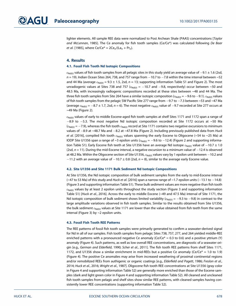
Two final observations from our fish tooth Nd data support the persistent export of deep waters from theAntarctic shelves during the early to middle Eocene: (1) the Nd isotope records from high-latitude Site 738and more northerly Site 757 (Figure 1) follow the same trend towards more radiogenic εNd(t) values duringthe early to middle Eocene and (2) a consistent Nd isotope gradient of ~1 εNd unit exists between these

Figure 5. Compilation of (i) published Eocene authigenic Nd isotope data for the (top) Pacific (gray data points) and (bot-tom) Atlantic/Indian sectors of the Southern Ocean (gray data points) and (ii) new data generated for this study (pelagicsites only; colored data points). Global benthic foramaninifer δ18O stack from Cramer et al. [2009] (Figure 5, top). NorthPacific data: Hague et al. [2012] and Thomas [2004]. Equatorial Pacific data: Thomas et al. [2008, 2014], van de Flierdt et al.[2004], Ling et al. [1997, 2005], and Le Houedec et al. [2016]. South Pacific data: Thomas et al. [2014], Scher et al.[2015], and this study. Atlantic/Indian Ocean data: Martin and Scher [2006], Scher and Martin [2004, 2006], Thomas et al.[2003], and this study. Modern day Ross Sea Bottom Water (RSBW, gray shading) and Circumpolar Deep Water (CDW, blueshading) εNd values taken from Rickli et al. [2014] and Stichel et al. [2012]. Modern Wilkes Land/Adélie Coast Bottom Water(WL-ACBW, gray shaded bar) εNd values from Lambelet et al. [2014].

Paleoceanography 10.1002/2017PA003135

HUCK ET AL. EOCENE SOUTHERN OCEAN CIRCULATION 682

two sites across a south-to-north transect, with lower values at southern Site 738 (Figure 5), suggesting asource to the south. We speculate that entrainment and export of Antarctic shelf-sourced waters to theIndian Ocean study sites likely occurred in geostrophically driven deep western boundary currents [e.g.,Scher et al., 2014] (Figure 7) and is consistent with several proxy-based [e.g., Corfield and Norris, 1996;Cramer et al., 2009; Katz et al., 2011; Pak and Miller, 1992; Sexton et al., 2006; Zachos et al., 1992, 1994] andmodel-based studies [e.g., Bice et al., 1997; Douglas et al., 2014; Uenzelmann-Neben et al., 2016].

5.2. Eocene Circulation and Origin of Deep Water Masses in the Southwest Pacific

Fish tooth εNd(t) values from Site 277 in the SW Pacific sector of the Southern Ocean range from�7.3 to �9.7and are similar to those recorded at Indian Ocean sites but are ~2 epsilon units lower on average than EoceneεNd(t) values from other Pacific Ocean sites (εNd(t) = �1.8 to �6.3 between 34 and 55 Ma) [Le Houedec et al.,2016; Ling et al., 1997, 2005; Hague et al., 2012; Thomas, 2004; Thomas et al., 2008, 2014; Scher et al., 2015;van de Flierdt et al., 2004] (Figures 5 and 6). This observation is noteworthy, as the Tasman Gateway was fullyclosed or only open to very shallow circulation during the early andmiddle Eocene [Bijl et al., 2013b]. Changesin dinoflagellate assemblages at Site U1356 between 48 and 49Ma [Bijl et al., 2013b] have been interpreted asa shallow opening of the Tasman Gateway, with waters flowing from the SW Pacific into the AAG under theinfluence of prevailing winds from the east [e.g., Huber et al., 2004]. Furthermore, younger fish tooth Nd iso-tope records from the region indicate an intermediate to deep (~500 to 2500 m) water flow from the Pacificto the Indian Ocean through the gateway in the late Eocene. Consistent with these observations, we note thatthe negative εNd(t) values recorded at Site 277 during the early to middle Eocene predate even the earliestopening event in the region. We conclude that it is unlikely that the unradiogenic intermediate/deep watersat Site 277 were the result of eastward transport from the Indian Ocean sector through the Tasman Gatewayto the Ross Sea region during the early to middle Eocene.

Instead, we propose two alternative options for the unradiogenic character of waters at Site 277: (1) an influxof intermediate/deep waters from the Indian Ocean via the Indonesian seaway or (2) local formation ofintermediate/deep waters in the Ross Sea region. Through the Cretaceous to Eocene, the low-latitude sea-ways were characterized by a strong, westward flowing surface current. These waters flowed from thePacific Ocean through the Indonesian seaway and across continental seaways in the Tethys to the Atlanticbasin [e.g., Jovane et al., 2009; Pucéat et al., 2005; Poulsen et al., 1999; Soudry et al., 2006]. Radiogenic

Figure 6. Global sites from the Atlantic, Indian, Pacific, and Southern Ocean basins, where seawater Nd isotope data havebeen generated for the early to middle Eocene time interval (~54–40 Ma). Data from literature denoted using circlescolor coded by Nd isotopic composition. New data generated in this study denoted by stars. The published ≤40 Ma recordfor Site 757 [Martin and Scher, 2006] has been extended in this study back to the early Eocene. Atlantic Ocean data:Scher and Martin [2006], Scher and Martin [2004], Via and Thomas [2006], Thomas et al. [2003],MacLeod et al. [2011],Martinet al. [2012], Burton et al. [1997], and O0Nions et al. [1998]. Indian Ocean data: Martin and Scher [2006] and Thomas et al.[2003]. Pacific Ocean data: Ling et al. [1997, 2005], Hague et al. [2012], Thomas [2004], and Thomas et al. [2008, 2014].Tectonic reconstruction made using Ocean Drilling Stratigraphic Network online toolkit (www.odsn.de).

Paleoceanography 10.1002/2017PA003135

HUCK ET AL. EOCENE SOUTHERN OCEAN CIRCULATION 683

seawater Nd isotope compositions are reconstructed at depth from the Pacific side of the IndonesianGateway throughout the Eocene (εNd(t) = �5.9 to �4.6) [Le Houedec et al., 2016], in contrast to moreunradiogenic values reconstructed at Site 213 in the Indian Ocean [Thomas et al., 2003] (Figure 6). Aconsistent radiogenic-unradiogenic trend from the Pacific to the Indian Ocean basins suggests a westwardflow of intermediate/deep waters also characterized the region during the Eocene. We therefore considerIndian Ocean waters flowing through the Indonesian seaway an unlikely explanation for the unradiogenicNd values recorded at SW Pacific Site 277.

The dominantly radiogenic Nd isotopic composition of Pacific deep waters during the Eocene (Figure 5) havepersisted since at least ~110 Ma [e.g., Robinson et al., 2010] and reflect the influx of Nd from young volcanicrocks around the Pacific rim [e.g., Goldstein and Jacobsen, 1988; Jeandel et al., 2007]. In contrast, outcroppingbedrock around the pre-Eocene continental margins of the SW Pacific contains a significant amount of olderterranes (i.e., Proterozoic basement and Paleozoic granitoids and metasediments of the Australian andAntarctic margins) [Cook et al., 2013; Pankhurst et al., 1998; Roberts et al., 2013] as well as youngerMesozoic volcanics, providing a range in εNd values that extends to quite unradiogenic Nd isotopic composi-tions (εNd(t) ~�4 to�20) [Cook et al., 2013; Gingele and De Deckker, 2005]. This range of bedrock Nd composi-tions provides a suitable source region for the seawater Nd isotopic compositions recorded at Site 277(Figure 5).

Based on the distribution of geological source regions surrounding the Pacific Ocean basin, the unradiogeniccharacter of fish tooth Nd isotope values from Site 277 suggests formation of intermediate/deep waters inthe SW Pacific region during the early and middle Eocene, most likely the Ross Sea region, in agreement withexisting modeling and proxy-based studies [e.g., Hollis et al., 2012; Huber et al., 2004; Thomas et al., 2014]. Wealso note that fish tooth εNd records from the Central Pacific suggest a significant contribution of unradio-genic deep waters (paleodepths of 2300 to 2900 m) originating from the Ross Sea (South Pacific DeepWater, SPDW) during the early Eocene [e.g., Thomas et al., 2003, 2014].

However, Site 277 εNd(t) values (�7.3 to �9.7) are lower than both Eocene seawater Nd isotope distributionsmodeled by Thomas et al. [2014] for the SW Pacific (εNd(t) = ~ � 6.5 to �6.0) and modern day values of RossSea bottom water (εNd = �7.4 to �6.5) [Rickli et al., 2014]. One possible explanation is that the Nd isotopiccomposition of RSBW has changed through time. This is feasible due to the Oligocene, and younger,emplacement ages of the late Cenozoic McMurdo Volcanic Group in broad areas around the Ross Sea[e.g., McIntosh, 2000]. Clear evidence for a major change in the composition of erosional inputs to theRoss Sea, containing material from this young, volcanic source, is provided in the Cape Roberts cores[Roberts et al., 2013] and could have readily affected local seawater, driving it toward more radiogenic

Figure 7. Simplified intermediate/deep water mass circulation in the Southern Ocean during the early to middle Eocene asinterpreted from this study. Study sites (stars) and water masses (arrows) are color coded to average εNd(t) valuesfrom this study for the 54–40 Ma interval, with the exception of Sites 689 and 1090 (~40–43 Ma) [Scher and Martin, 2004,2006, 2008] and Site 213 [Thomas et al., 2003]. Double-headed arrows represent εNd(t) values of Eocene sediment fromAntarctic and Australian hinterland [Cook et al., 2013; Gingele and De Deckker, 2005; this study]. Tectonic reconstructionmade using Ocean Drilling Stratigraphic Network online toolkit (www.odsn.de).

Paleoceanography 10.1002/2017PA003135

HUCK ET AL. EOCENE SOUTHERN OCEAN CIRCULATION 684

Nd isotopic compositions since the Oligocene/Miocene. Unfortunately, there are currently no Eocene-ageddeep/bottom water Nd data (>1500 m paleodepth) from the SW Pacific region, and, as such, we are unableto conclude whether the intermediate/deep waters at Site 277 were ultimately exported from the region asdeeper flowing SPDW or whether a more stratified water column prevailed with unradiogenic watersreconstructed from Site 277 overlying a more radiogenic proto-RSBW [e.g., Thomas et al., 2014].

5.3. The Role of Ocean Circulation in the Termination of the EECO

A notable feature of our new early and middle Eocene fish tooth Nd records is the occurrence of a pro-nounced excursion in εNd(t) values between 50 and 48 Ma at multiple sites located in the southern IndianOcean, Australo-Antarctic Gulf, and SW Pacific Ocean. The most unradiogenic Nd isotopic compositions areobserved at Sites 738, 757, 1171, and U1356 and coincide with the end of extreme global warmth duringthe EECO, falling within the early/middle Eocene Transition (EMET; ~51–47 Ma; Figure 5). The EMET is charac-terized by global cooling of deep ocean temperatures, sea level lowstands, and widespread deep marinesediment hiatuses [e.g., Browning et al., 1996; Hohbein et al., 2012; Kominz et al., 2008; Miller et al., 1987;Pekar et al., 2005; Zachos et al., 2008]. A drop in atmospheric pCO2 concentrations, potentially driven byincreased silicate weathering, may explain global cooling [e.g., Anagnostou et al., 2016; Kent and Muttoni,2008, 2013], while tectonic reorganization such as the shallow opening of the Tasman Gateway at ~48 Mamay have also caused regional cooling [Bijl et al., 2013b]. Below we further explore the origin of the fish toothNd excursions from sites in the Tasman Gateway region and the potential relationship between these excur-sions and the cooling climate trend following the EECO.5.3.1. Shallow Opening of the Tasman GatewayBased on early to middle Eocene marine microfossil and organic geochemical records from Site U1356, Bijlet al. [2013b] interpreted a shallow opening of the Tasman Gateway during the EMET. The associated influxof Pacific-sourced surface waters to the Australo-Antarctic Gulf is proposed to have resulted in regional cool-ing along the East Antarctic margin. There was likely long-term deepening of Site U1356 from ~500 m to~1000 m during the early to middle Eocene [Bijl et al., 2013b; Escutia et al., 2011], but precise paleodepth esti-mates for the site are uncertain. Given the uncertainty of the paleodepth of Site U1356 at the EMET, it is pos-sible that a shallow influx of Pacific waters through the Tasman Gateway may not have been detected in ourfish tooth Nd isotope record. If the arrival of Pacific-sourced waters was captured by fish tooth samples at SiteU1356, we would expect a step change in Nd isotopes toward more radiogenic compositions, similar to εNd(t)values observed at Sites 1171 and 1172 (which have average Eocene εNd(t) values of �6.6 ± 2.2 (2sd, n = 23)).We do not observe such as shift during the mid-Eocene interval at Site U1536, but instead a transient excur-sion to unradiogenic compositions in fish tooth Nd isotopes away from, and subsequently returning to, theaverage Nd isotopic composition defined by the early Eocene and Oligocene sections of the record (Figure 2).This suggests that a different mechanism than the shallow opening of the Tasman Gateway was responsiblefor the change in seawater chemistry at Site U1356 during the EMET.5.3.2. Changes in the Erosional Regime on Antarctica: Influence on Shallow Marine RecordsThe observed transient negative Nd isotope excursion in our fish tooth record at Site U1356 is also recordedon the Pacific side of the Tasman Gateway at Site 1171, but not at Site 1172. Two excursions in the fish toothNd isotopes at Site 1171 at ~48 and ~ 49 Ma are of a similar magnitude (~ 2 εNd) to Site U1356 with respectiveεNd(t) (MIN) values of �12.4 at Site U1356 and �8.9 at Site 1171 at ~48 Ma (Figure 2) (note that there is uncer-tainty in the age of the excursion at Site 1171 (±0.5 Myr) due the low resolution of the age model; see sup-porting information for age model details). A similar additional excursion in seawater chemistry may haveoccurred at Site U1356. If it did, it was not recovered due to the hiatus between ~51 and ~49 Ma. Water massmixing alone cannot be responsible for these observed excursions as no suitably unradiogenic water masshas been documented within the respective surrounding oceanic areas during the Eocene (Figure 6).However, Eocene bulk sediment Nd data at both sites are lower than the associated fish tooth records(U1356 sediment εNd(t) = �13.1 to �14.7; 1171 sediment εNd(t) = �9.3 to �9.8; Figure 3), reflecting the localbedrock composition around the areas of Wilkes Land, Adélie Coast and Northern Victoria Land (for a sum-mary see Pierce et al. [2014]). We therefore conclude that changes in the erosional regime of the proximalgeological source regions is likely to be responsible for the Nd isotope excursions detected at Sites U1356and 1171. Relating the transient excursions in our fish tooth Nd records at Sites U1356 and 1171 to changingerosional fluxes from the Antarctic continent is also consistent with the absence of an excursion at Site 1172

Paleoceanography 10.1002/2017PA003135

HUCK ET AL. EOCENE SOUTHERN OCEAN CIRCULATION 685

between 48 and 49 Ma, as tectonic reconstructions place Site 1172 further north on the East Tasman Plateau[Cande and Stock, 2004; Figure 1].

We speculate that a period of intense erosion of the respective Antarctic source regions adjacent to SitesU1356 and 1171 (Figure 3) could have resulted in an increased flux of dissolved (and particulate) Nd to theshelf waters, modifying the composition of local waters toward the sedimentary Nd end-member. A similarmechanism was proposed by Scher et al. [2011] who suggested that the rapid growth and associated erosionof an ice sheet on Antarctica resulted in a pulse of unradiogenic Nd delivered to the Southern Ocean acrossthe Eocene-Oligocene transition. Increased continental erosion may have occurred as a result of either higherprecipitation levels or ephemeral glaciation in mountainous regions. Sediment Nd data alone cannot deci-pher which of these mechanisms was responsible for our records over the EMET. Our findings do, however,suggest that there may have been an important perturbation to the hydrological cycle on the Antarctic con-tinent over this interval, which is expressed in the chemistry of the surrounding ocean.5.3.3. Evidence for a Cooling Event During the EMET?Constraining the erosional mechanism responsible for the Nd isotope excursion in our fish tooth records atSites U1356 and 1171 relies on understanding the continental climate on Antarctica at the time. There is evi-dence for significant cooling during the EMET at both local and regional levels in the southern high latitudes,which may suggest that the development of small-scale highland ice sheets was a feasible driver for chan-ging erosional conditions during the EMET. At Site U1356, bulk sediment geochemistry suggests a short-liveddecrease in temperature and precipitation between 49 and 48 Ma [Passchier et al., 2013] within same intervalas the excursion in fish tooth Nd values. More regionally, a drop in deep water and sea surface temperaturesat Site 277 and an increase in the deposition of siliciclastic sediments has also been reported from the mid-Waipara section in New Zealand at ~48.5 Ma [e.g., Creech et al., 2010; Hollis et al., 2009, 2012]. These regionalresponses to a transient cooling event on the Antarctic continent are superimposed on a prolonged environ-mental shift in the southern high latitudes from the early to middle Eocene. Fossil pollen extracted from SiteU1356 sediments indicate a changing vegetation assemblage from high diversity plant ecosystems on theAntarctic continent during the early Eocene to a lower diversity, cooler assemblage in the middle Eocene[Contreras et al., 2013; Pross et al., 2012]. Similar terrestrial ecosystem changes have been reported from othersites around East Antarctica, the Antarctic Peninsula, and Southern Australia [e.g., Askin, 2000; Francis et al.,2008; Martin, 2006; Truswell and Macphail, 2009].

Farther afield, the fish tooth Nd records from pelagic Sites 738 and 757 also reach minimum εNd(t) values dur-ing the EMET interval (Figure 2). The observation of a similar excursion in the fish tooth Nd record at Site 738(located at ~62°S during the Eocene) to the shallow records from the Tasman Gateway implies that the pro-posed erosional event was widespread across East Antarctica. A similar record from Site 757 then furtherraises the question of whether the changes in Antarctic continental climate were propagated viaintermediate/deep ocean currents to lower latitudes. If so, what was the associated impact? IncreasedSouthern Ocean deep water export between 49 and 48 Ma has been inferred before in order to explainrecords of intensified bottom water currents and decreasing temperatures in the Atlantic and PacificOcean basins [e.g., Barron et al., 2015; Bralower et al., 1995; Danelian et al., 2007; Norris et al., 2001; Ortizand Thomas, 2015; Thomas et al., 2008]. The unradiogenic εNd(t) values between ~49 and 48 Ma at Sites738 and 757 (Figure 5) may therefore be indicative of both an altered Nd isotopic composition of southernsourced seawater due to increased delivery of unradiogenic Nd to the surrounding continental shelves, aswell as cooling in locations of deep water formation, resulting in invigorated propagation of SouthernOcean deep waters into the major ocean basins. Ultimately, to better understand the cause-or-consequencenature between Antarctic continental erosion, cooling over the EMET, and reinvigorated deep ocean circula-tion requires focused studies from cores with well-constrained age models across this little-studied, but pivo-tal, interval in Cenozoic climate history.

6. Conclusion

New Nd isotope data from fossil fish teeth and bulk sediments from pelagic and shallow marine settings inthe Tasman region and surrounding areas of the Southern Ocean allow reconstruction of the distributionof intermediate/deep water masses during the early to middle Eocene. These data isotopically fingerprintthe Antarctic shelves as the source of unradiogenic Nd isotope values that characterize the Indian Ocean

Paleoceanography 10.1002/2017PA003135

HUCK ET AL. EOCENE SOUTHERN OCEAN CIRCULATION 686

sector of the Southern Ocean and deep waters of the Indian Ocean during the Eocene. Additionally, we iden-tify a new, locally formed intermediate-deep water mass in the Ross Sea region during the early to middleEocene, but further research is required to conclude whether this unradiogenic deep water is exported fromthe SW Pacific or constitutes a specific layer in a stratified water column in the Ross Gyre. Finally, transientexcursions in the fish tooth Nd isotope records at shallowmarine sites U1356 and 1171 and pelagic, but prox-imal, Site 738 identify a period of increased flux of Nd from widespread locations on the Antarctic continentto the surrounding shelf seas. Results from Indian Ocean pelagic Site 757 furthermore suggest that this shelfwater was then transported northward in intermediate/deep water masses. The increase in continental ero-sion on Antarctica potentially results from changes in the hydrological cycle in association with regional cool-ing documented at other regional and global locations between ~49 and 48 Ma during the EMET. Climaticchanges on the Antarctic continent during the Eocene greenhouse may hence be communicated in deepwaters across ocean basins, potentially influencing climate on a larger, global scale.

ReferencesAnagnostou, E., E. H. John, K. M. Edgar, G. L. Foster, A. Ridgwell, G. N. Inglis, R. D. Pancost, D. J. Lunt, and P. N. Pearson (2016), Changing

atmospheric CO2 concentration was the primary driver of early Cenozoic climate, Nature, 533(7603), 380–384.Arsouze, T., J. Dutay, F. Lacan, and C. Jeandel (2009), Reconstructing the Nd oceanic cycle using a coupled dynamical-biogeochemical model,

Biogeosciences, 6(12), 2829–2846.Askin, R. A. (2000), Spores and pollen from the McMurdo sound erratics, Antarctica, Antarct. Res. Ser., 76, 161–181.Barron, J., et al. (1989), Proceedings of the Ocean Drilling Program: Initial Reports, vol. 119, 942 pp.Barron, J. A., C. E. Stickley, and D. Bukry (2015), Paleoceanographic, and paleoclimatic constraints on the global Eocene diatom and silico-

flagellate record, Palaeogeogr. Palaeoclimatol. Palaeoecol., 422, 85–100.Bice, K. L., E. J. Barron, and W. H. Peterson (1997), Continental runoff and early Cenozoic bottom-water sources, Geology, 25(10), 951–954.Bijl, P. K., S. Schouten, A. Sluijs, G. J. Reichart, J. C. Zachos, and H. Brinkhuis (2009), Early Palaeogene temperature evolution of the southwest

Pacific Ocean, Nature, 461(7265), 776–779.Bijl, P. K., A. Sluijs, and H. Brinkhuis (2013a), A magneto- and chemostratigraphically calibrated dinoflagellate cyst zonation of the early

Paleogene South Pacific Ocean, Earth Sci. Rev., 124, 1–31.Bijl, P. K., J. A. Bendle, S. M. Bohaty, J. Pross, S. Schouten, L. Tauxe, C. E. Stickley, R. M. McKay, U. Röhl, and M. Olney (2013b), Eocene cooling

linked to early flow across the Tasmanian Gateway, Proc. Natl. Acad. Sci. U.S.A., 110(24), 9645–9650.Boyle, E. A., and L. Keigwin (1985), Comparison of Atlantic and Pacific paleochemical records for the last 215, 000 years: Changes in deep

ocean circulation and chemical inventories, Earth Planet. Sci. Lett., 76, 135–150.Bohaty, S. M., and J. C. Zachos (2003), Significant Southern Ocean warming event in the late middle Eocene, Geology, 31(11), 1017–1020.Bohaty, S. M., J. C. Zachos, F. Florindo, and M. L. Delaney (2009), Coupled greenhouse warming and deep-sea acidification in the middle

Eocene, Paleoceanography, 24, PA2207, doi:10.1029/2008PA001676.Borrelli, C., B. S. Cramer, and M. E. Katz (2014), Bipolar Atlantic deepwater circulation in the middle-late Eocene: Effects of Southern Ocean

gateway openings, Paleoceanography, 29, 308–327, doi:10.1002/2012PA002444.Bralower, T. J., J. C. Zachos, E. Thomas, M. Parrow, C. K. Paull, D. C. Kelly, I. P. Silva, W. V. Sliter, and K. C. Lohmann (1995), Late Paleocene to

Eocene paleoceanography of the equatorial Pacific Ocean: Stable isotopes recorded at ocean drilling program site 865, Allison Guyot,Paleoceanography, 10, 841–865, doi:10.1029/95PA01143.

Brass, G. W., J. R. Southam, and W. H. Peterson (1982), Warm saline bottom water in the ancient ocean, Nature, 296, 620–623.Browning, J. V., K. G. Miller, and D. K. Pak (1996), Global implications of lower to middle Eocene sequence boundaries on the New Jersey

coastal plain: The icehouse cometh, Geology, 24(7), 639–642.Burton, K. W., H. F. Ling, and R. K. O’Nions (1997), Closure of the Central American Isthmus and its effect on deep-water formation in the North

Atlantic, Nature, 386, 382–385.Cande, S. C., and J. M. Stock (2004), Cenozoic reconstructions of the Australia-New Zealand-South Pacific sector of Antarctica, in The Cenozoic

Southern Ocean: Tectonics, Sedimentation, and Climate Change Between Australia and Antarctica, edited by N. F. Exon, J. P. Kennett, and M.J. Malone, pp. 5–18, AGU, Washington, D. C.

Chavagnac, V., J. Milton, D. Green, J. Breuer, O. Bruguier, D. Jacob, T. Jong, G. Kamenov, J. Le Huray, and Y. Liu (2007), Towards the devel-opment of a fossil bone geochemical standard: An inter-laboratory study, Anal. Chim. Acta, 599(2), 177–190.

Contreras, L., J. Pross, P. K. Bijl, A. Koutsodendris, J. I. Raine, B. van de Schootbrugge, and H. Brinkhuis (2013), Early to middle Eocene vege-tation dynamics at the Wilkes Land Margin (Antarctica), Rev. Palaeobot. Palynol., 197, 119–142.

Cook, C. P., T. van de Flierdt, T. Williams, S. R. Hemming, M. Iwai, M. Kobayashi, F. J. Jimenez-Espejo, C. Escutia, J. J. González, and B.-K. Khim(2013), Dynamic behaviour of the East Antarctic ice sheet during Pliocene warmth, Nat. Geosci., 6(9), 765–769.

Corfield, R. M., and R. D. Norris (1996), Deep water circulation in the Paleocene ocean, in Correlation of the Early Paleogene in North-WestEurope, edited by R. W. O’B. Knox, R. M. Corfield, and R. E. Dunay, Geol. Soc. London Spec. Publ., vol. 101, pp. 443–456.

Coxall, H. K., P. A. Wilson, H. Palike, C. H. Lear, and J. Backman (2005), Rapid stepwise onset of Antarctic glaciation and deeper calcite com-pensation in the Pacific Ocean, Nature, 433(7021), 53–57.

Cramer, B., J. Toggweiler, J. Wright, M. Katz, and K. Miller (2009), Ocean overturning since the Late Cretaceous: Inferences from a new benthicforaminiferal isotope compilation, Paleoceanography, 24, PA4216, doi:10.1029/2008PA001683.

Creech, J. B., J. A. Baker, C. J. Hollis, H. E. Morgans, and E. G. Smith (2010), Eocene sea temperatures for the mid-latitude southwest Pacific fromMg/Ca ratios in planktonic and benthic foraminifera, Earth Planet. Sci. Lett., 299(3), 483–495.

Danelian, T., S. Saint Martin, and M.-M. Blanc-Valleron (2007), Middle Eocene radiolarian and diatom accumulation in the equatorial Atlantic(Demerara Rise, ODP Leg 207): Possible links with climatic and palaeoceanographic changes, C. R. Palevol, 6(1–2), 103–114.

De Baar, H. J., M. P. Bacon, P. G. Brewer, and K. W. Bruland (1985), Rare earth elements in the Pacific and Atlantic Oceans, Geochim.Cosmochim. Acta, 49(9), 1943–1959.

DeConto, R. M., and D. Pollard (2003), Rapid Cenozoic glaciation of Antarctica induced by declining atmospheric CO2,Nature, 421(6920), 245–249.

Paleoceanography 10.1002/2017PA003135

HUCK ET AL. EOCENE SOUTHERN OCEAN CIRCULATION 687

AcknowledgmentsWe gratefully acknowledge K. Kreissigand B. Coles for laboratory and technicalsupport and Diederik Liebrand for manyhelpful discussions. We thank the Editorand reviewers for their constructivefeedback, which has improved thismanuscript. This research used samplesand data provided by IODP. Funding forthis research was provided by NERCgrants awarded to T.v.d.F. (NE/L004607/1)and T.v.d.F. and S.M.B. (NE/I006257/1)and an ECORD Research Grant awardedto C.E.H. All data used for this study areavailable in the supporting information,cited references, and on the Pangaeadatabase (www.pangaea.de). Theauthors declare no conflicting interests.

Douglas, P. M. J., H. P. Affek, L. C. Ivany, A. J. P. Houben, W. P. Sijp, A. Sluijs, S. Schouten, andM. Pagani (2014), Pronounced zonal heterogeneityin Eocene southern high-latitude sea surface temperatures, Proc. Natl. Acad. Sci. U.S.A., 111(18), 6582–6587.

Dunkley Jones, T., P. R. Bown, P. N. Pearson, B. S. Wade, H. K. Coxall, and C. H. Lear (2008), Major shifts in calcareous phytoplankton assem-blages through the Eocene-Oligocene transition of Tanzania and their implications for low-latitude primary production,Paleoceanography, 23, PA4204, doi:10.1029/2008PA001640.

Ehrmann, W. U., M. Melles, G. Kuhn, and H. Grobe (1992), Significance of clay mineral assemblages in the Antarctic Ocean, Mar. Geol., 107(4),249–273.

Elderfield, H., and R. Pagett (1986), Rare earth elements in ichthyoliths: Variations with redox conditions and depositional environment, Sci.Total Environ., 49, 175–197.

Escutia, C., H. Brinkhius, A. Klaus, and the Expedition 318 Scientists (2011), Proceedings of the IODP, vol. 18.Exon, N., J. P. Kennett, M. J. Malone, and the Expedition 189 Scientists (2001), The Tasmanian gateway: Cenozoic climatic and oceanographic

development, Sites 1168-1172 Rep., Ocean Drilling Program.Francis, J. E., et al. (2008), Chapter 8 from greenhouse to icehouse—The Eocene/Oligocene, in Antarctica, in Developments in Earth and

Environmental Sciences, edited by F. Fabio, and S. Martin, pp. 309–368, Elsevier, Netherlands.Freslon, N., G. Bayon, S. Toucanne, S. Bermell, C. Bollinger, S. Chéron, J. Etoubleau, Y. Germain, A. Khripounoff, and E. Ponzevera (2014), Rare

earth elements and neodymium isotopes in sedimentary organic matter, Geochim. Cosmochim. Acta, 140, 177–198.Galeotti, S., et al. (2016), Antarctic Ice Sheet variability across the Eocene-Oligocene boundary climate transition, Science, 352(6281),

76–80.German, C. R., and H. Elderfield (1990), Application of the Ce anomaly as a paleoredox indicator: The ground rules, Paleoceanography, 5,

823–833, doi:10.1029/PA005i005p00823.Gingele, F., and P. De Deckker (2005), Clay mineral, geochemical and Sr–Nd isotopic fingerprinting of sediments in the Murray–Darling fluvial

system, southeast Australia, Aust. J. Earth Sci., 52(6), 965–974.Goldstein, S. J., and S. B. Jacobsen (1988), Nd and Sr isotopic systematics of river water suspended material: Implications for crustal evolution,

Earth Planet. Sci. Lett., 87, 249–265.Goldner, A., N. Herold, and M. Huber (2014), Antarctic glaciation caused ocean circulation changes at the Eocene-Oligocene transition,

Nature, 511, 574–577.Hague, A. M., D. J. Thomas, M. Huber, R. Korty, S. C. Woodard, and L. B. Jones (2012), Convection of North Pacific deep water during the early

Cenozoic, Geology, 40(6), 527–530.Hayes, D. E., et al. (1975), Initial reports of the Deep Sea Drilling Project, vol. 28, pp. 725–759, U.S. Gov. Print. Off., Washington, D. C.Hohbein, M. W., P. F. Sexton, and J. A. Cartwright (2012), Onset of North Atlantic Deepwater production coincident with inception of the

Cenozoic global cooling trend, Geology, 40(3), 255–258.Hollis, C. J., D. B. Waghorn, C. P. Strong, E. M. Crouch (1997), Integrated Paleogene biostratigraphy of DSDP site 277 (Leg 29): Foraminifera,

calcareous nannofossils, Radiolaria, and palynomorphs, Institute of Geological and Nuclear Sciences Science Report, 97/07, 87 pp.Hollis, C. J., L. Handley, E. M. Crouch, H. E. Morgans, J. A. Baker, J. Creech, K. S. Collins, S. J. Gibbs, M. Huber, and S. Schouten (2009), Tropical sea

temperatures in the high-latitude South Pacific during the Eocene, Geology, 37(2), 99–102.Hollis, C. J., et al. (2012), Early Paleogene temperature history of the Southwest Pacific Ocean: Reconciling proxies and models, Earth Planet.

Sci. Lett., 349–350, 53–66.Hollis, C. J., B. R. Hines, K. Littler, V. Villasante-Marcos, D. K. Kulhanek, C. P. Strong, J. C. Zachos, S. M. Eggins, L. Northcote, and A. Phillips (2015),

The Paleocene–Eocene Thermal Maximum at DSDP Site 277, Campbell Plateau, southern Pacific Ocean, Clim. Past, 11(7), 1009–1025.Houben, A. J. P., et al. (2013), Reorganization of Southern Ocean plankton ecosystem at the onset of Antarctic glaciation, Science, 340(6130),

341–344.Huber, M., and R. Caballero (2011), The early Eocene equable climate problem revisted, Clim. Past, 7, 603–633.Huber, M., and D. Nof (2006), The ocean circulation in the southern hemisphere and its climatic impacts in the Eocene, Palaeogeogr.

Palaeoclimatol. Palaeoecol., 231(1), 9–28.Huber, M., and L. C. Sloan (2001), Heat transport, deep waters, and thermal gradients: Coupled simulation of an Eocene greenhouse climate,

Geophys. Res. Lett., 28, 3481–3484, doi:10.1029/2001GL012943.Huber, B. T., and F. Quillévéré (2005), Revised Paleogene planktonic foraminiferal biozonation for the Austral realm, J. Foraminifer. Res., 35(4),

299–314.Huber, M., H. Brinkhuis, C. E. Stickley, K. Döös, A. Sluijs, J. Warnaar, S. A. Schellenberg, and G. L. Williams (2004), Eocene circulation of the

Southern Ocean: Was Antarctica kept warm by subtropical waters?, Paleoceanography, 19, PA4026, doi:10.1029/2004PA001014.Huck, C. E., T. van de Flierdt, F. J. Jiménez-Espejo, S. M. Bohaty, U. Röhl, and S. J. Hammond (2016), Robustness of fossil fish teeth for seawater

neodymium isotope reconstructions under variable redox conditions in an ancient shallow marine setting, Geochem. Geophys. Geosyst.,17, 679–698, doi:10.1002/2015GC006218.

Jacobsen, S. B., and G. Wasserburg (1980), Sm-Nd isotopic evolution of chondrites, Earth Planet. Sci. Lett., 50(1), 139–155.Jeandel, C., T. Arsouze, F. Lacan, P. Téchiné, and J.-C. Dutay (2007), Isotopic Nd compositions and concentrations of the lithogenic inputs into

the ocean: A compilation, with an emphasis on the margins, Chem. Geol., 239, 156–164.Jovane, L., R. Coccioni, A. Marsili and G. Acton (2009), The late Eocene greenhouse–icehouse transition: Observations from the Massignano

global stratotype section and point (GSSP), in The Late Eocene Earth—Hothouse, Ice-House, and Impacts, edited by C. Koeberl andA. Montanari, Geol. Soc. Am. Spec. Pap., 452, pp. 149–168.

Katz, M. E., B. S. Cramer, J. Toggweiler, G. Esmay, C. Liu, K. G. Miller, Y. Rosenthal, B. S. Wade, and J. D. Wright (2011), Impact of AntarcticCircumpolar current development on late Paleogene ocean structure, Science, 332(6033), 1076–1079.

Kennett, J. P. (1977), Cenozoic evolution of Antarctic glaciation, the Circum-Antarctic Ocean, and their impact on global paleoceanography,J. Geophys. Res., 82, 3843–3860, doi:10.1029/JC082i027p03843.

Kennett, J. P., et al. (1975), Initial reports of the Deep Sea Drilling project, vol. 29, 1186 pp.Kennett, J. P., and L. D. Stott (1991), Abrupt deep sea warming, paleoceanographic changes and benthic extinctions at the end of the

Paleocene, Nature, 353, 319–322.Kent, D. V., and G. Muttoni (2008), Equatorial convergence of India and early Cenozoic climate trends, Proc. Natl. Acad. Sci. U.S.A., 105(42),

16,065–16,070.Kent, D. V., and G. Muttoni (2013), Modulation of Late Cretaceous and Cenozoic climate by variable drawdown of atmospheric pCO2 from

weathering of basaltic provinces on continents drifting through the equatorial humid belt, Clim. Past, 9(2), 525–546.Kominz, M., J. Browning, K. Miller, P. Sugarman, S. Mizintseva, and C. Scotese (2008), Late Cretaceous to Miocene sea-level estimates from the

New Jersey and Delaware coastal plain coreholes: An error analysis, Basin Res., 20(2), 211–226.

Paleoceanography 10.1002/2017PA003135

HUCK ET AL. EOCENE SOUTHERN OCEAN CIRCULATION 688

Lambelet, M., T. van de Flierdt, E. C. V. Butler, A. R. Bowie, S. R. Rintoul, R. J. Watson, T. Remenyl, and D. Lannuzel (2014), The Nd isotopiccompositions of Adélie coast bottom water—Insights from GIPY6 cruise along 1400 , Abstract OS21G-07 presented at 2014 Fall Meeting2014, AGU, San Francisco, Calif.

Lawver, L. A., and L. M. Gahagan (2003), Evolution of Cenozoic seaways in the circum-Antarctic region, Palaeogeogr. Palaeoclimatol.Palaeoecol., 198(1), 11–37.

Le Houedec, S., L. Meynadier, and C. J. Allègre (2016), Seawater Nd isotope variation in the Western Pacific Ocean since 80 Ma (ODP 807,Ontong Java Plateau), Mar. Geol., 380, 138–147.

Lear, C. H., T. R. Bailey, P. N. Pearson, H. K. Coxall, and Y. Rosenthal (2008), Cooling and ice growth across the Eocene-Oligocene transition,Geology, 36(3), 251–254.

Ling, H. F., K. W. Burton, R. K. O’Nions, B. S. Kamber, F. von Blanckenburg, A. J. Gibb, and J. R. Hein (1997), Evolution of Nd and Pb isotopes inCentral Pacific seawater from ferromanganese crusts, Earth Planet. Sci. Lett., 146(1–2), 1–12.

Ling, H. F., S.-Y. Jiang, M. Frank, H.-Y. Zhou, F. Zhou, Z.-L. Lu, X.-M. Chen, Y.-H. Jiang, and C.-D. Ge (2005), Differing controls over the CenozoicPb and Nd isotope evolution of deepwater in the central North Pacific Ocean, Earth Planet. Sci. Lett., 232, 345–361.

Littler, K., U. Röhl, T. Westerhold, and J. C. Zachos (2014), A high-resolution benthic stable-isotope record for the South Atlantic: Implicationsfor orbital-scale changes in Late Paleocene–early Eocene climate and carbon cycling, Earth Planet. Sci. Lett., 401, 18–30.

Liu, Z. H., M. Pagani, D. Zinniker, R. DeConto, M. Huber, H. Brinkhuis, S. R. Shah, R. M. Leckie, and A. Pearson (2009), Global cooling during theEocene-Oligocene climate transition, Science, 323(5918), 1187–1190.

Lunt, D. J., P. J. Valdes, T. Dunkley-Jones, A. Ridgwell, A. M. Haywood, D. N. Schmidt, R. Marsh, and M. Maslin (2010), CO2-driven ocean cir-culation changes as an amplifier of Paleocene-Eocene thermal maximum hydrate destabilization, Geology, 38(10), 875–878.

MacLeod, K. G., C. Isaza-Londoño, E. E. Martin, A. Jimenez Berrocoso, C. Basak (2011), Changes in North Atlantic circulation at the end of theCretaceous greenhouse interval, Nat. Geosci., 4, 779–782.

Martin, E. E., and B. A. Haley (2000), Fossil fish teeth as proxies for seawater Sr and Nd isotopes, Geochim. Cosmochim. Acta, 64(5), 835–847.Martin, E. E., and H. Scher (2006), A Nd isotopic study of southern sourced waters and Indonesian throughflow at intermediate depths in the

Cenozoic Indian Ocean, Geochem. Geophys. Geosyst., 7, Q09N02, doi:10.1029/2006GC001302.Martin, E., K. Macleod, A. Jiménez Berrocoso and E. Bourbon (2012), Water mass circulation on Demerara Rise during the Late Cretaceous

based on Nd isotopes, Earth Planet. Sci. Lett., 327, 111–120.Martin, H. (2006), Cenozoic climatic change and the development of the arid vegetation in Australia, J. Arid Environ., 66(3), 533–563.McIntosh, W. C. (2000),

40Ar/

39Ar geochronology of tephra and volcanic clasts in CRP-2A, Victoria Land Basin, Antarctica, Terra Antarct., 7,

621–630.Miller, K. G., R. G. Fairbanks, and G. S. Mountain (1987), Tertiary oxygen isotope synthesis, sea level history, and continental margin erosion,

Paleoceanography, 2, 1–19, doi:10.1029/PA002i001p00001.Moiroud, M., E. Pucéat, Y. Donnadieu, G. Bayon, K. Moriya, J.-F. Deconinck, and M. Boyet (2013), Evolution of the neodymium isotopic sig-

nature of neritic seawater on a northwestern Pacific margin: New constrains on possible end-members for the composition of deep-watermasses in the Late Cretaceous ocean, Chem. Geol., 356, 160–170.

Norris, R. D., A. Klaus, and D. Kroon (2001), Mid-Eocene deep water, the Late Palaeocene thermal maximum and continental slope masswasting during the Cretaceous-Palaeogene impact, Geol. Soc. London Spec. Publ., 183(1), 23–48.

O’Nions, R. K., M. Frank, F. von Blanckenburg and H. F. Ling (1998), Secular variation of Nd and Pb isotopes in ferromanganese crusts from theAt- lantic, Indian and Pacific Oceans, Earth Planet. Sci. Lett., 155, 15–28.

Orsi, A. H., and C. L. Wiederwohl (2009), A recount of Ross Sea waters, Deep Sea Res., Part II, 56(13), 778–795.Ortiz, S., and E. Thomas (2015), Deep-sea benthic foraminiferal turnover during the early–middle Eocene transition at Walvis Ridge

(SE Atlantic), Palaeogeogr. Palaeoclimatol. Palaeoecol., 417, 126–136.Otto-Bliesner, B. L., E. C. Brady, and C. Shields (2002), Late Cretaceous ocean: Coupled simulations with the National Center for Atmospheric

Research Climate System Model, J. Geophys. Res., 107(D2), 4019, doi:10.1029/2001JD000821.Pagani, M., J. C. Zachos, K. H. Freeman, B. Tipple, and S. Bohaty (2005), Marked decline in atmospheric carbon dioxide concentrations during

the Paleogene, Science, 309(5734), 600–603.Pagani, M., M. Huber, Z. Liu, S. M. Bohaty, J. Henderiks, W. Sijp, S. Krishnan, and R. M. DeConto (2011), The role of carbon dioxide during the

onset of Antarctic glaciation, Science, 334(6060), 1261–1264.Pak, D. K., and K. G. Miller (1992), Paleocene to Eocene benthic foraminiferal isotopes and assemblages: Implications for deepwater circu-

lation, Paleoceanography, 7, 405–422, doi:10.1029/92PA01234.Pankhurst, R. J., S. D. Weaver, J. D. Bradshaw, B. C. Storey, and T. R. Ireland (1998), Geochronology and geochemistry of pre-Jurassic super-

terranes in Marie Byrd Land, Antarctica, J. Geophys. Res., 103, 2529–2547, doi:10.1029/97JB02605.Passchier, S., S. M. Bohaty, F. Jiménez-Espejo, J. Pross, U. Röhl, T. van de Flierdt, C. Escutia, and H. Brinkhuis (2013), Early Eocene to middle

Miocene cooling and aridification of East Antarctica, Geochem. Geophys. Geosyst., 14, 1399–1410, doi:10.1002/ggge.20106.Passchier, S., D. J. Ciarletta, T. E. Miriagos, P. K. Bijl, and S. M. Bohaty (2017), An Antarctic stratigraphic record of stepwise ice growth through

the Eocene-Oligocene transition, Geol. Soc. Am. Bull., 29(3/4), 318–330.Peirce, J., et al. (1989), Proceedings of the Ocean Drilling Project: Initial Reports, vol. 121, pp. 359–453, Ocean Drilling Program, College Station,

Tex.Pekar, S. F., A. Hucks, M. Fuller, and S. Li (2005), Glacioeustatic changes in the early and middle Eocene (51–42 Ma): Shallow-water strati-

graphy from ODP Leg 189 Site 1171 (South Tasman Rise) and deep-sea δ18O records, Geol. Soc. Am. Bull., 117(7–8), 1081–1093.Pucéat, E., C. Lécuyer, and L. Reisberg (2005), Neodymium isotope evolution of NW Tethyan upper ocean waters throughout the Cretaceous,

Earth Planet. Sci. Lett., 236, 705–720.Pierce, E., S. Hemming, T. Williams, T. van de Flierdt, S. Thomson, P. Reiners, G. Gehrels, S. Brachfeld, and S. Goldstein (2014), A comparison of

detrital U–Pb zircon, 40 Ar/39 Ar hornblende, 40 Ar/39 Ar biotite ages in marine sediments off East Antarctica: Implications for the geologyof subglacial terrains and provenance studies, Earth Sci. Rev., 138, 156–178.

Pierce, E. L., T. Williams, T. Flierdt, S. R. Hemming, S. L. Goldstein, and S. A. Brachfeld (2011), Characterizing the sediment provenance of EastAntarctica’s weak underbelly: The Aurora and Wilkes sub-glacial basins, Paleoceanography, 26, PA4217, doi:10.1029/2011PA002127.

Pin, C., and J. S. Zalduegui (1997), Sequential separation of light rare-earth elements, thorium and uranium by miniaturized extractionchromatography: Application to isotopic analyses of silicate rocks, Anal. Chim. Acta, 339(1), 79–89.

Poulsen, C. J., E. J. Barron, C. C. Johnson, and P. Fawcett (1999), Links between major climatic factors and regional oceanic circulation in themid-Cretaceous, Geol. Soc. Am. Spec. Pap., 73–90.

Pross, J., L. Contreras, P. K. Bijl, D. R. Greenwood, S. M. Bohaty, S. Schouten, J. A. Bendle, U. Röhl, L. Tauxe, and J. I. Raine (2012), Persistent near-tropical warmth on the Antarctic continent during the early Eocene epoch, Nature, 488(7409), 73–77.

Paleoceanography 10.1002/2017PA003135

HUCK ET AL. EOCENE SOUTHERN OCEAN CIRCULATION 689

Rickli, J., M. Gutjahr, D. Vance, M. Fischer-Gödde, C.-D. Hillenbrand, and G. Kuhn (2014), Neodymium and hafnium boundary contributions toseawater along the West Antarctic continental margin, Earth Planet. Sci. Lett., 394, 99–110.

Roberts, A. P., F. Florindo, G. Villa, L. Chang, L. Jovane, S. M. Bohaty, J. C. Larrasoaña, D. Heslop, and J. D. Fitz Gerald (2011), Magnetotacticbacterial abundance in pelagic marine environments is limited by organic carbon flux and availability of dissolved iron, Earth Planet. Sci.Lett., 310, 441–452.

Roberts, A. P., L. Sagnotti, F. Florindo, S. M. Bohaty, K. L. Verosub, G. S. Wilson, and J. C. Zachos (2013), Environmental record of paleoclimate,unroofing of the Transantarctic Mountains, and volcanism in later Eocene to early Miocene glaci-marine sediments from the Victoria LandBasin, Ross Sea, Antarctica, J. Geophys. Res. Solid Earth, 118, 1845–1861, doi:10.1002/jgrb.50151.

Robinson, S. A., D. P. Murphy, D. Vance, and D. J. Thomas (2010), Formation of “Southern Component Water” in the Late Cretaceous: Evidencefrom Nd-isotopes, Geology, 38, 871–874.

Scher, H. D., and E. E. Martin (2004), Circulation in the Southern Ocean during the Paleogene inferred from neodymium isotopes, Earth Planet.Sci. Lett., 228(3–4), 391–405.

Scher, H. D., and E. E. Martin (2006), Timing and climatic consequences of the opening of Drake Passage, Science, 312(5772), 428–430.Scher, H. D., and E. E. Martin (2008), Oligocene deep water export from the North Atlantic and the development of the Antarctic Circumpolar

Current examined with neodymium isotopes, Paleoceanography, 23, PA1205, doi:10.1029/2006PA001400.Scher, H. D., and M. L. Delaney (2010), Breaking the glass ceiling for high resolution Nd isotope records in early Cenozoic paleoceanography,

Chem. Geol., 269(3), 329–338.Scher, H. D., S. M. Bohaty, J. C. Zachos, and M. L. Delaney (2011), Two-stepping into the icehouse: East Antarctic weathering during pro-

gressive ice-sheet expansion at the Eocene–Oligocene transition, Geology, 39(4), 383–386.Scher, H. D., S. M. Bohaty, B. W. Smith, and G. H. Munn (2014), Isotopic interrogation of a suspected late Eocene glaciation, Paleoceanography,

29, 628–644, doi:10.1002/2014PA002648.Scher, H. D., J. M. Whittaker, S. E. Williams, J. C. Latimer, W. E. Kordesch, and M. L. Delaney (2015), Onset of Antarctic Circumpolar Current 30

million years ago as Tasmanian Gateway aligned with westerlies, Nature, 523(7562), 580–583.Sexton, P. F., P. A. Wilson, and R. D. Norris (2006), Testing the Cenozoic multisite composite δ18O and δ13C curves: Newmonospecific Eocene

records from a single locality, Demerara Rise (Ocean Drilling Program Leg 207), Paleoceanography, 21, PA2019, doi:10.1029/2005PA001253.

Sexton, P. F., R. D. Norris, P. A. Wilson, H. Pälike, T. Westerhold, U. Röhl, C. T. Bolton, and S. Gibbs (2011), Eocene global warming events drivenby ventilation of oceanic dissolved organic carbon, Nature, 471(7338), 349–352.

Shaw, H., and G. Wasserburg (1985), Sm-Nd in marine carbonates and phosphates: Implications for Nd isotopes in seawater and crustal ages,Geochim. Cosmochim. Acta, 49(2), 503–518.

Sijp, W. P., and M. H. England (2016), The effect of low ancient greenhouse temperature gradients on the ocean’s overturning circulation,Clim. Past, 12, 543–552.

Sijp, W. P., M. H. England, and M. Huber (2011), Effect of the deepening of the Tasman Gateway on the global ocean, Paleoceanography, 26,PA4207, doi:10.1029/2011PA002143.

Soudry, D., C. R. Glenn, Y. Nathan, I. Segal, and D. Vonder Haar (2006), Evolution of Tethyan phosphogenesis along the northern edges of theArabian-African shield during the Cretaceous-Eocene as deduced from temporal variations of Ca and Nd isotopes and rates of P accu-mulation, Earth Sci. Rev., 78, 27–57.

Stichel, T., M. Frank, J. Rickli, and B. A. Haley (2012), The hafnium and neodymium isotope composition of seawater in the Atlantic sector ofthe Southern Ocean, Earth Planet. Sci. Lett., 317, 282–294.

Stille, P., and H. Fischer (1990), Secular variation in the isotopic composition of Nd in Tethys seawater, Geochim. Cosmochim. Acta, 54,3139–3145.

Tachikawa, K., V. Athias, and C. Jeandel (2003), Neodymium budget in the modern ocean and paleo-oceanographic implications, J. Geophys.Res., 108(8), 3254, doi:10.1029/1999JC000285.

Tanaka, T., et al. (2000), JNdi-1: A neodymium isotopic reference in consistency with LaJolla neodymium, Chem. Geol., 168, 279–281.Tauxe, L., C. Stickley, S. Sugisaki, P. Bijl, S. Bohaty, H. Brinkhuis, C. Escutia, J. Flores, A. Houben, and M. Iwai (2012), Chronostratigraphic

framework for the IODP Expedition 318 cores from the Wilkes Land Margin: Constraints for paleoceanographic reconstruction,Paleoceanography, 27, PA2214, doi:10.1029/2012PA002308.

Taylor, S. R., and S. M. McLennan (1985), The Continental Crust: Its Composition and Evolution, 312 pp., Blackwell Scientific Publ.,Oxford, U. K.

Thomas, D. J. (2004), Evidence for deep-water production in the North Pacific Ocean during the early Cenozoic warm interval, Nature,430(6995), 65–68.

Thomas, D. J., T. J. Bralower, and C. E. Jones (2003), Neodymium isotopic reconstruction of late Paleocene-early Eocene thermohalinecirculation, Earth Planet. Sci. Lett., 209(3–4), 309–322.

Thomas, D. J., M. Lyle, T. C. Moore, and D. K. Rea (2008), Paleogene deepwater mass composition of the tropical Pacific and implications forthermohaline circulation in a greenhouse world, Geochem. Geophys. Geosyst., 9, Q02002, doi:10.1029/2007GC001748.

Thomas, D. J., R. Korty, M. Huber, J. A. Schubert, and B. Haines (2014), Nd isotopic structure of the Pacific Ocean 70–30 Ma and numericalevidence for vigorous ocean circulation and ocean heat transport in a greenhouse world, Paleoceanography, 29, 454–469, doi:10.1002/2013PA002535.

Truswell, E. M., and M. K. Macphail (2009), Polar forests on the edge of extinction: What does the fossil spore and pollen evidence from EastAntarctica say?, Aust. Syst. Bot., 22(2), 57–106.

Uenzelmann-Neben, G., T. Weber, J. Grützner, and M. Thomas (2016), Transition from the Cretaceous ocean to Cenozoic circulation in thewestern South Atlantic—A twofold reconstruction, Tectonophysics, doi:10.1016/j.tecto.2016.05.036.

van de Flierdt, T., S. R. Hemming, S. L. Goldstein, and W. Abouchami (2006), Radiogenic isotope fingerprint of Wilkes Land–Adélie coastbottom water in the circum-Antarctic Ocean, Geophys. Res. Lett., 33, L12606, doi:10.1029/2006GL026020.

van de Flierdt, T., M. Frank, A. N. Halliday, J. R. Hein, B. Hattendorf, D. Günther, and P. W. Kubik (2004), Deep and bottomwater export from theSouthern Ocean to the Pacific over the past 38 million years, Paleoceanography, 19, PA1020, doi:10.1029/2003PA000923.

van Hinsbergen, D. J., L. V. de Groot, S. J. van Schaik, W. Spakman, P. K. Bijl, A. Sluijs, C. G. Langereis, and H. Brinkhuis (2015), A paleolatitudecalculator for paleoclimate studies, PLoS One, 10(6), e0126946.

Vandenberghe, N., R. P. Speijer, and F. J. Hilgen (2012), The Paleogene period, in The Geologic Time Scale 2012, edited by F. M. Gradstein et al.,pp. 855–922, Elsevier, Amsterdam.

Via, R. K., and D. J. Thomas (2006), Evolution of Atlantic thermohaline circulation: Early Oligocene onset of deep-water production in theNorth Atlantic, Geology, 34(6), 441–444.

Paleoceanography 10.1002/2017PA003135

HUCK ET AL. EOCENE SOUTHERN OCEAN CIRCULATION 690

Weis, D., et al. (2006), High-precision isotopic characterization of USGS reference materials by TIMS and MC-ICP-MS, Geochem. Geophys.Geosyst., 7, Q08006, doi:10.1029/2006GC001283.

Wright, J., H. Schrader, and W. T. Holser (1987), Paleoredox variations in ancient oceans recorded by rare earth elements in fossil apatite,Geochim. Cosmochim. Acta, 51(3), 631–644.

Zachos, J., D. Rea, K. Seto, N. Niitsuma, and R. Nomura (1992), Paleogene and early Neogene deep water history of the Indian Ocean:Inferences from stable isotopic records, in The Indian Ocean: A Synthesis of Results from the Ocean Drilling Program, Geophys. Monogr.,vol. 70, pp. 351–386, AGU, Washington, D. C.

Zachos, J., M. Pagani, L. Sloan, E. Thomas, and K. Billups (2001), Trends, rhythms, and aberrations in global climate 65 Ma to present, Science,292(5517), 686–693.

Zachos, J. C., L. D. Stott, and K. C. Lohmann (1994), Evolution of early Cenozoic marine temperatures, Paleoceanography, 9, 353–387,doi:10.1029/93PA03266.

Zachos, J. C., G. R. Dickens, and R. E. Zeebe (2008), An early Cenozoic perspective on greenhouse warming and carbon-cycle dynamics,Nature, 451(7176), 279–283.

Paleoceanography 10.1002/2017PA003135

HUCK ET AL. EOCENE SOUTHERN OCEAN CIRCULATION 691