UNIVERSIT ´ E LIBRE DE BRUXELLES FACULT ´ E DES S CIENCES APPLIQU ´ EES Ant Colony Optimization and its Application to Adaptive Routing in Telecommunication Networks Gianni Di Caro Dissertation pr´ esent´ ee en vue de l’obtention du grade de Docteur en Sciences Appliqu´ ees Bruxelles, September 2004 PROMOTEUR:PROF.MARCO DORIGO IRIDIA, Institut de Recherches Interdisciplinaires et de D´ eveloppements en Intelligence Artificielle ANN ´ EE ACAD ´ EMIQUE 2003-2004

Welcome message from author
This document is posted to help you gain knowledge. Please leave a comment to let me know what you think about it! Share it to your friends and learn new things together.
Transcript
UNIVERSITE LIBRE DE BRUXELLES
FACULTE DES SCIENCES APPLIQUEES
Ant Colony Optimization and its Application to
Adaptive Routing in Telecommunication Networks
Gianni Di Caro
Dissertation presentee en vue de l’obtention du grade de
Docteur en Sciences Appliquees
Bruxelles, September 2004
PROMOTEUR: PROF. MARCO DORIGO
IRIDIA, Institut de Recherches Interdisciplinaires
et de Developpements en Intelligence Artificielle
ANNEE ACADEMIQUE 2003-2004

Abstract
In ant societies, and, more in general, in insect societies, the activities of the individuals, as well
as of the society as a whole, are not regulated by any explicit form of centralized control. On the
other hand, adaptive and robust behaviors transcending the behavioral repertoire of the single
individual can be easily observed at society level. These complex global behaviors are the result
of self-organizing dynamics driven by local interactions and communications among a number
of relatively simple individuals. The simultaneous presence of these and other fascinating and
unique characteristics have made ant societies an attractive and inspiring model for building
new algorithms and newmulti-agent systems. In the last decade, ant societies have been taken as a
reference for an ever growing body of scientific work, mostly in the fields of robotics, operations
research, and telecommunications.
Among the different works inspired by ant colonies, theAnt Colony Optimization metaheuristic
(ACO) is probably the most successful and popular one. The ACOmetaheuristic is a multi-agent
framework for combinatorial optimization whose main components are: a set of ant-like agents,
the use of memory and of stochastic decisions, and strategies of collective and distributed learning.
It finds its roots in the experimental observation of a specific foraging behavior of some ant
colonies that, under appropriate conditions, are able to select the shortest path among few possi-
ble paths connecting their nest to a food site. The pheromone, a volatile chemical substance laid
on the ground by the ants while walking and affecting in turn their moving decisions according
to its local intensity, is the mediator of this behavior. All the elements playing an essential role
in the ant colony foraging behavior were understood, thoroughly reverse-engineered and put
to work to solve problems of combinatorial optimization by Marco Dorigo and his co-workers
at the beginning of the 1990’s. From that moment on it has been a flourishing of new com-
binatorial optimization algorithms designed after the first algorithms of Dorigo’s et al., and of
related scientific events. In 1999 the ACO metaheuristic was defined by Dorigo, Di Caro and
Gambardella with the purpose of providing a common framework for describing and analyzing
all these algorithms inspired by the same ant colony behavior and by the same common process
of reverse-engineering of this behavior. Therefore, the ACO metaheuristic was defined a poste-
riori, as the result of a synthesis effort effectuated on the study of the characteristics of all these
ant-inspired algorithms and on the abstraction of their common traits. The ACO’s synthesis
was also motivated by the usually good performance shown by the algorithms (e.g., for several
important combinatorial problems like the quadratic assignment, vehicle routing and job shop
scheduling, ACO implementations have outperformed state-of-the-art algorithms).
The definition and study of the ACOmetaheuristic is one of the two fundamental goals of the
thesis. The other one, strictly related to this former one, consists in the design, implementation,
and testing of ACO instances for problems of adaptive routing in telecommunication networks.
This thesis is an in-depth journey through the ACO metaheuristic, during which we have
(re)defined ACO and tried to get a clear understanding of its potentialities, limits, and relation-
ships with other frameworks and with its biological background. The thesis takes into account
all the developments that have followed the original 1999’s definition, and provides a formal and
comprehensive systematization of the subject, as well as an up-to-date and quite comprehensive
review of current applications. We have also identified in dynamic problems in telecommuni-
cation networks the most appropriate domain of application for the ACO ideas. According to
this understanding, in the most applicative part of the thesis we have focused on problems of
adaptive routing in networks and we have developed and tested four new algorithms.
Adopting an original point of view with respect to the way ACO was firstly defined (but
maintaining full conceptual and terminological consistency), ACO is here defined and mainly
discussed in the terms of sequential decision processes andMonte Carlo sampling and learning. More
precisely, ACO is characterized as a policy search strategy aimed at learning the distributed pa-
rameters (called pheromone variables in accordance with the biological metaphor) of the stochastic
decision policy which is used by so-called ant agents to generate solutions. Each ant represents
in practice an independent sequential decision process aimed at constructing a possibly feasible so-
lution for the optimization problem at hand by using only information local to the decision step.
Ants are repeatedly and concurrently generated in order to sample the solution set according to the
current policy. The outcomes of the generated solutions are used to partially evaluate the current
policy, spot the most promising search areas, and update the policy parameters in order to possibly
focus the search in those promising areas while keeping a satisfactory level of overall exploration.
This way of looking at ACO has facilitated to disclose the strict relationships between ACO
and other well-known frameworks, like dynamic programming, Markov and non-Markov decision
processes, and reinforcement learning. In turn, this has favored reasoning on the general properties
of ACO in terms of amount of complete state informationwhich is used by the ACO’s ants to take
optimized decisions and to encode in pheromone variables memory of both the decisions that
belonged to the sampled solutions and their quality.
The ACO’s biological context of inspiration is fully acknowledged in the thesis. We report
with extensive discussions on the shortest path behaviors of ant colonies and on the identifi-
cation and analysis of the few nonlinear dynamics that are at the very core of self-organized
behaviors in both the ants and other societal organizations. We discuss these dynamics in the
general framework of stigmergic modeling, based on asynchronous environment-mediated com-
munication protocols, and (pheromone) variables priming coordinated responses of a number
of “cheap” and concurrent agents.
The second half of the thesis is devoted to the study of the application of ACO to problems
of online routing in telecommunication networks. This class of problems has been identified in the
thesis as the most appropriate for the application of the multi-agent, distributed, and adaptive
nature of the ACO architecture. Four novel ACO algorithms for problems of adaptive routing in
telecommunication networks are throughly described. The four algorithms cover a wide spec-
trum of possible types of network: two of them deliver best-effort traffic in wired IP networks, one
is intended for quality-of-service (QoS) traffic in ATM networks, and the fourth is for best-effort traf-
fic in mobile ad hoc networks. The two algorithms for wired IP networks have been extensively
tested by simulation studies and compared to state-of-the-art algorithms for a wide set of refer-
ence scenarios. The algorithm for mobile ad hoc networks is still under development, but quite
extensive results and comparisons with a popular state-of-the-art algorithm are reported. No
results are reported for the algorithm for QoS, which has not been fully tested. The observed ex-
perimental performance is excellent, especially for the case of wired IP networks: our algorithms
always perform comparably or much better than the state-of-the-art competitors. In the thesis
we try to understand the rationale behind the brilliant performance obtained and the good level
of popularity reached by our algorithms. More in general, we discuss the reasons of the general
efficacy of the ACO approach for network routing problems compared to the characteristics of
more classical approaches. Moving further, we also informally define Ant Colony Routing (ACR),
a multi-agent framework explicitly integrating learning components into the ACO’s design in
order to define a general and in a sense futuristic architecture for autonomic network control.
Most of the material of the thesis comes from a re-elaboration of material co-authored and
published in a number of books, journal papers, conference proceedings, and technical reports.
The detailed list of references is provided in the Introduction.
Acknowledgments
First, I shall thank the ants! Without those little mates bugging around this thesis simply would
have not happened. When I was a little kid, I was kind of concerned about the little ant-hills
and their tiny inhabitants sprouting all over my garden. So, one day, I started thinking that
during the winter they could feel cold, and I unilaterally decided to equip their primitive nests
with a technologically advanced heating system. Therefore, I started drilling and putting pipes
underground, connecting the pipes to faucets and sinks, and letting hot water passing through
in order to warm up my little mates during the cold winter days. How disappointed I was
when I realized that they didn’t appreciate my heating technology and quite in a short time they
just vanished, likely moving their nests somewhere else! Well, actually, I then tried to let my
adorable cat to enjoy my concerns about cold and I brought my now well consolidated heating
technology into the carton box where he was used to spend, sleeping, most of his precious time.
Unfortunately, he too didn’t seem ready to enjoy the pleasures of technology, so I gave up and
focused on other amenities. . . So, I do really feel now that in a sense my little mates had actually
appreciated those maybe a bit awkward efforts and rewarded me back, laying somewhere in the
universe the pheromone trail that led me to Marco Dorigo and his ant-inspired algorithms. He’s
the person I shall thank the more for what is in this thesis, and for really bugging me to write it!
The content of the thesis covers part of the research work that I’ve done during the last six
years. These years have been a long journey into science and into life. I’vemoved first to Brussels
(IRIDIA), then to Japan (ATR), then back to Belgium (IRIDIA again), and finally to Lugano, in
Switzerland (IDSIA). All these places have been great places to work and enjoy life. They are
fully international environments where I had the chance to make really good friends and to meet
so many great scientists from whom I could really learn so much! I want to thank for this the
directors of these laboratories where I have been (Philippe Smets, Hugues Bersini and Marco
Dorigo, Katsunori Shimohara, Kenji Doya, and Luca Gambardella) who have done and are still
doing a great job!
This thesis is really the outgrowth of all the discussions, brainstorming, collaborations, that
have happened during these years. It’s like a puzzle, whose tiles have been added day by day:
after a discussion in front of several beers, or after attending a seminar about how Japanese
can learn to distinguish between the sounds “lock” and “rock”, or after a long telephone call
with some friend thousands of kilometers far away discussing about markov decision processes
or antibodies at 3am. . . Thinking back, I realize that I should thank so many people across the
world, but they are really too many. I want to mention here just few of them, those who con-
sciously or unconsciously (!), in different ways, have had a major impact on my growth as a
scientist. The list is in (stochastic) order of appearance: Alessandro Saffiotti, Bruno Marchal, Vit-
torio Gorrini, Marco Dorigo, Hugues Bersini, Gianluca Bontempi, Katsunori Shimohara, Kenji
Doya, Thomas Halva Labella, Luca Maria Gambardella, and Frederick Ducatelle.
There are also few very special people that I really want to mention (in strict alphabetic order,
this time). They have been the closest ones, the most important ones, either from a scientific
point of view and/or from a personal point view. To them a really special “Grazie!” goes deep
down from my heart: Carlotta Piscopo, Luca Di Mauro, Masako (Maco-chan) Hosomi, Mauro
Birattari, Silvana Valensin. I hope there’ll always be a trail of pheromone somewhere in the
universe to find each other.
To this list of very special people I must add my mother, always there to listen to my misfor-
tunes, to give me a warm word, to encourage me, and who gave me the first real impetus to sit
down and write the first words of this thesis: “Grazie Mamma!”.
A special thank goes also to Luca Gambardella, who very kindly let me also to work at the
thesis while I was/am in his group at IDSIA, and who has always been a source of valuables
suggestions and points of view.
Part of the work in this thesis was supported by two Marie Curie fellowships (contract n.
CEC-TMR ERBFMBICT 961153 and HPMF-CT-2000-00987) awarded to the author by the scien-
tific institutions of the European Community. The information provided is the sole responsibility
of the author and does not reflect the Community’s opinion. The Community is not responsible
for any use that might be made of data appearing in this thesis.
Contents
List of Figures xii
List of Tables xiii
List of Algorithms xv
List of Examples xvii
List of Abbreviations xix
1 Introduction 1
1.1 Goals and scientific contributions . . . . . . . . . . . . . . . . . . . . . . . . . . . . . 4
1.1.1 General goals of the thesis . . . . . . . . . . . . . . . . . . . . . . . . . . . . . 4
1.1.2 Theoretical and practical relevance of the thesis’ goals . . . . . . . . . . . . . 6
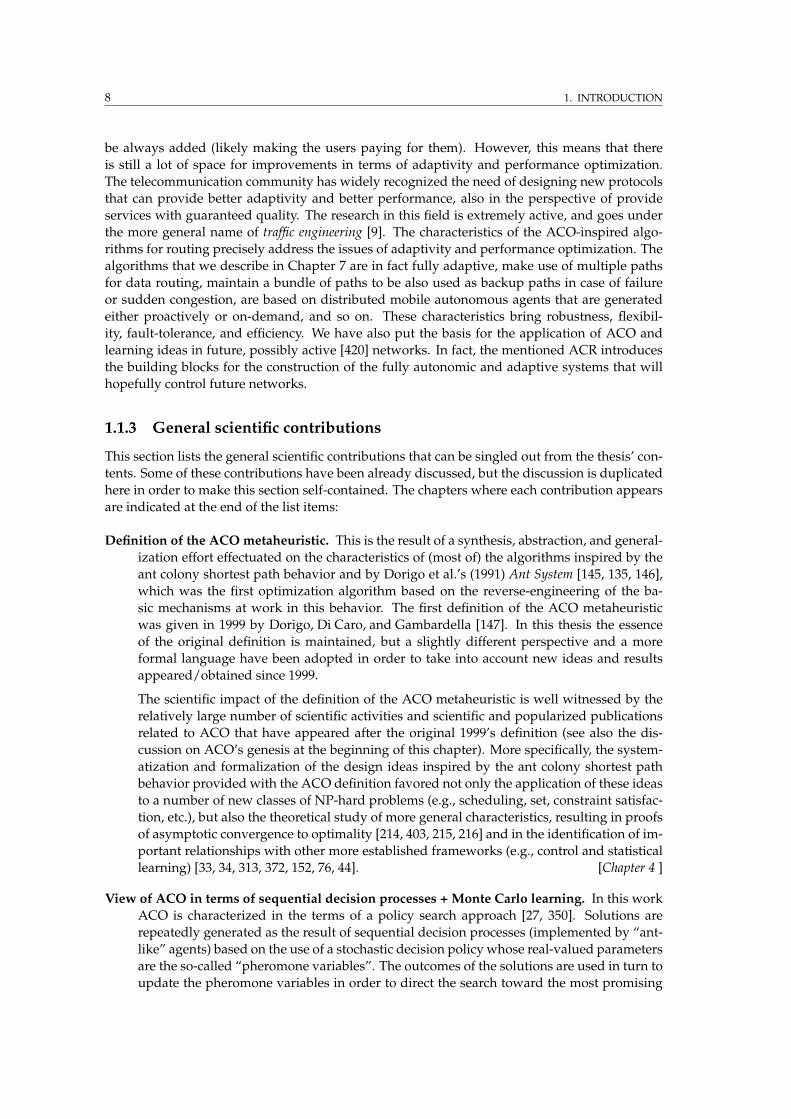
1.1.3 General scientific contributions . . . . . . . . . . . . . . . . . . . . . . . . . . 8
1.2 Organization and published sources of the thesis . . . . . . . . . . . . . . . . . . . . 10
1.3 ACO in a nutshell: a preliminary and informal definition . . . . . . . . . . . . . . . 17
I From real ant colonies to the Ant Colony Optimization metaheuristic 21
2 Ant colonies, the biological roots of Ant Colony Optimization 23
2.1 Ants colonies can find shortest paths . . . . . . . . . . . . . . . . . . . . . . . . . . . 24
2.2 Shortest paths as the result of a synergy of ingredients . . . . . . . . . . . . . . . . . 27
2.3 Robustness, adaptivity, and self-organization properties . . . . . . . . . . . . . . . . 30
2.4 Modeling ant colony behaviors using stigmergy: the ant way . . . . . . . . . . . . . 31
2.5 Summary . . . . . . . . . . . . . . . . . . . . . . . . . . . . . . . . . . . . . . . . . . . 34
3 Combinatorial optimization, construction methods, and decision processes 37
3.1 Combinatorial optimization problems . . . . . . . . . . . . . . . . . . . . . . . . . . 39
3.1.1 Solution components . . . . . . . . . . . . . . . . . . . . . . . . . . . . . . . . 43
3.1.2 Characteristics of problem representations . . . . . . . . . . . . . . . . . . . 44
3.2 Construction methods for combinatorial optimization . . . . . . . . . . . . . . . . . 46
3.2.1 Strategies for component inclusion and feasibility issues . . . . . . . . . . . 49
3.2.2 Appropriate domains of application for construction methods . . . . . . . . 51
3.3 Construction processes as sequential decision processes . . . . . . . . . . . . . . . . 52
3.3.1 Optimal control and the state of a construction/decision process . . . . . . 54
3.3.2 State graph . . . . . . . . . . . . . . . . . . . . . . . . . . . . . . . . . . . . . 56
3.3.3 Construction graph . . . . . . . . . . . . . . . . . . . . . . . . . . . . . . . . . 61
3.3.4 The general framework of Markov decision processes . . . . . . . . . . . . . 67
3.3.5 Generic non-Markov processes and the notion of phantasma . . . . . . . . . 72
viii CONTENTS
3.4 Strategies for solving optimization problems . . . . . . . . . . . . . . . . . . . . . . 75
3.4.1 General characteristics of optimization strategies . . . . . . . . . . . . . . . 76
3.4.2 Dynamic programming and the use of state-value functions . . . . . . . . . 80
3.4.3 Approximate value functions . . . . . . . . . . . . . . . . . . . . . . . . . . . 87
3.4.4 The policy search approach . . . . . . . . . . . . . . . . . . . . . . . . . . . . 88
3.5 Summary . . . . . . . . . . . . . . . . . . . . . . . . . . . . . . . . . . . . . . . . . . . 92
4 The Ant Colony Optimization Metaheuristic (ACO) 95
4.1 Definition of the ACO metaheuristic . . . . . . . . . . . . . . . . . . . . . . . . . . . 97
4.1.1 Problem representation and pheromone model exploited by ants . . . . . . 98
4.1.1.1 State graph and solution feasibility . . . . . . . . . . . . . . . . . . 98
4.1.1.2 Pheromone graph and solution quality . . . . . . . . . . . . . . . . 99
4.1.2 Behavior of the ant-like agents . . . . . . . . . . . . . . . . . . . . . . . . . . 102
4.1.3 Behavior of the metaheuristic at the level of the colony . . . . . . . . . . . . 107
4.1.3.1 Scheduling of the actions . . . . . . . . . . . . . . . . . . . . . . . . 108
4.1.3.2 Pheromone management . . . . . . . . . . . . . . . . . . . . . . . . 110
4.1.3.3 Daemon actions . . . . . . . . . . . . . . . . . . . . . . . . . . . . . 112
4.2 Ant System: the first ACO algorithm . . . . . . . . . . . . . . . . . . . . . . . . . . . 112
4.3 Discussion on general ACO’s characteristics . . . . . . . . . . . . . . . . . . . . . . 115
4.3.1 Optimization by using memory and learning . . . . . . . . . . . . . . . . . . 115
4.3.2 Strategies for pheromone updating . . . . . . . . . . . . . . . . . . . . . . . . 122
4.3.3 Shortest paths and implicit/explicit solution evaluation . . . . . . . . . . . 126
4.4 Revised definitions for the pheromone model and the ant-routing table . . . . . . . 128
4.4.1 Limits of the original definition . . . . . . . . . . . . . . . . . . . . . . . . . . 128
4.4.2 New definitions to use more and better pheromone information . . . . . . . 129
4.5 Summary . . . . . . . . . . . . . . . . . . . . . . . . . . . . . . . . . . . . . . . . . . . 134
5 Application of ACO to combinatorial optimization problems 137
5.1 ACO algorithms for problems that can be solved in centralized way . . . . . . . . . 140
5.1.1 Traveling salesman problems . . . . . . . . . . . . . . . . . . . . . . . . . . . 140
5.1.2 Quadratic assignment problems . . . . . . . . . . . . . . . . . . . . . . . . . 147
5.1.3 Scheduling problems . . . . . . . . . . . . . . . . . . . . . . . . . . . . . . . . 149
5.1.4 Vehicle routing problems . . . . . . . . . . . . . . . . . . . . . . . . . . . . . 151
5.1.5 Sequential ordering problems . . . . . . . . . . . . . . . . . . . . . . . . . . . 153
5.1.6 Shortest common supersequence problems . . . . . . . . . . . . . . . . . . . 154
5.1.7 Graph coloring and frequency assignment problems . . . . . . . . . . . . . 154
5.1.8 Bin packing and multi-knapsack problems . . . . . . . . . . . . . . . . . . . 156
5.1.9 Constraint satisfaction problems . . . . . . . . . . . . . . . . . . . . . . . . . 157
5.2 Parallel models and implementations . . . . . . . . . . . . . . . . . . . . . . . . . . 158
5.3 Related approaches . . . . . . . . . . . . . . . . . . . . . . . . . . . . . . . . . . . . . 160
5.4 Summary . . . . . . . . . . . . . . . . . . . . . . . . . . . . . . . . . . . . . . . . . . . 166
II Application of ACO to problems of adaptive routing intelecommunication networks169
6 Routing in telecommunication networks 171
6.1 Routing: Definition and characteristics . . . . . . . . . . . . . . . . . . . . . . . . . . 172
6.2 Classification of routing algorithms . . . . . . . . . . . . . . . . . . . . . . . . . . . . 174
6.2.1 Control architecture: centralized vs. distributed . . . . . . . . . . . . . . . . 175
6.2.2 Routing tables: static vs. dynamic . . . . . . . . . . . . . . . . . . . . . . . . 175
CONTENTS ix
6.2.3 Optimization criteria: optimal vs. shortest paths . . . . . . . . . . . . . . . . 177
6.2.4 Load distribution: single vs. multiple paths . . . . . . . . . . . . . . . . . . . 177
6.3 Metrics for performance evaluation . . . . . . . . . . . . . . . . . . . . . . . . . . . . 181
6.4 Main routing paradigms: Optimal and shortest path routing . . . . . . . . . . . . . 182
6.4.1 Optimal routing . . . . . . . . . . . . . . . . . . . . . . . . . . . . . . . . . . . 182
6.4.2 Shortest path routing . . . . . . . . . . . . . . . . . . . . . . . . . . . . . . . . 183
6.4.2.1 Distance-vector algorithms . . . . . . . . . . . . . . . . . . . . . . . 184
6.4.2.2 Link-state algorithms . . . . . . . . . . . . . . . . . . . . . . . . . . 187
6.4.3 Collective and individual rationality in optimal and shortest path routing . 190
6.5 An historical glance at the routing on the Internet . . . . . . . . . . . . . . . . . . . 192
6.6 Summary . . . . . . . . . . . . . . . . . . . . . . . . . . . . . . . . . . . . . . . . . . . 194
7 ACO algorithms for adaptive routing 197
7.1 AntNet: traffic-adaptive multipath routing for best-effort IP networks . . . . . . . 200
7.1.1 The communication network model . . . . . . . . . . . . . . . . . . . . . . . 202
7.1.2 Data structures maintained at the nodes . . . . . . . . . . . . . . . . . . . . . 205
7.1.3 Description of the algorithm . . . . . . . . . . . . . . . . . . . . . . . . . . . 208
7.1.3.1 Proactive ant generation . . . . . . . . . . . . . . . . . . . . . . . . 208
7.1.3.2 Storing information during the forward phase . . . . . . . . . . . . 210
7.1.3.3 Routing decision policy adopted by forward ants . . . . . . . . . . 210
7.1.3.4 Avoiding loops . . . . . . . . . . . . . . . . . . . . . . . . . . . . . . 212
7.1.3.5 Forward ants change into backward ants and retrace the path . . . 213
7.1.3.6 Updating of routing tables and statistical traffic models . . . . . . 214
7.1.3.7 Updates of all the sub-paths composing the forward path . . . . . 219
7.1.3.8 A complete example and pseudo-code description . . . . . . . . . 221
7.1.4 A critical issue: how to measure the relative goodness of a path? . . . . . . 221
7.1.4.1 Constant reinforcements . . . . . . . . . . . . . . . . . . . . . . . . 223
7.1.4.2 Adaptive reinforcements . . . . . . . . . . . . . . . . . . . . . . . . 224
7.2 AntNet-FA: improving AntNet using faster ants . . . . . . . . . . . . . . . . . . . . 226
7.3 Ant Colony Routing (ACR): a framework for autonomic network routing . . . . . 228
7.3.1 The architecture . . . . . . . . . . . . . . . . . . . . . . . . . . . . . . . . . . . 231
7.3.1.1 Node managers . . . . . . . . . . . . . . . . . . . . . . . . . . . . . 232
7.3.1.2 Active perceptions and effectors . . . . . . . . . . . . . . . . . . . . 237
7.3.2 Two additional examples of Ant Colony Routing algorithms . . . . . . . . . 238
7.3.2.1 AntNet+SELA: QoS routing in ATM networks . . . . . . . . . . . . 239
7.3.2.2 AntHocNet: routing in mobile ad hoc networks . . . . . . . . . . . 242
7.4 Related work on ant-inspired algorithms for routing . . . . . . . . . . . . . . . . . . 245
7.5 Summary . . . . . . . . . . . . . . . . . . . . . . . . . . . . . . . . . . . . . . . . . . . 254
8 Experimental results for ACO routing algorithms 257
8.1 Experimental settings . . . . . . . . . . . . . . . . . . . . . . . . . . . . . . . . . . . . 258
8.1.1 Topology and physical properties of the networks . . . . . . . . . . . . . . . 259
8.1.2 Traffic patterns . . . . . . . . . . . . . . . . . . . . . . . . . . . . . . . . . . . 261
8.1.3 Performance metrics . . . . . . . . . . . . . . . . . . . . . . . . . . . . . . . . 262
8.2 Routing algorithms used for comparison . . . . . . . . . . . . . . . . . . . . . . . . 263
8.2.1 Parameter values . . . . . . . . . . . . . . . . . . . . . . . . . . . . . . . . . . 265
8.3 Results for AntNet and AntNet-FA . . . . . . . . . . . . . . . . . . . . . . . . . . . . 266
8.3.1 SimpleNet . . . . . . . . . . . . . . . . . . . . . . . . . . . . . . . . . . . . . . 267
8.3.2 NSFNET . . . . . . . . . . . . . . . . . . . . . . . . . . . . . . . . . . . . . . . 268
8.3.3 NTTnet . . . . . . . . . . . . . . . . . . . . . . . . . . . . . . . . . . . . . . . . 270
x CONTENTS
8.3.4 6x6Net . . . . . . . . . . . . . . . . . . . . . . . . . . . . . . . . . . . . . . . . 274
8.3.5 Larger randomly generated networks . . . . . . . . . . . . . . . . . . . . . . 274
8.3.6 Routing overhead . . . . . . . . . . . . . . . . . . . . . . . . . . . . . . . . . . 276
8.3.7 Sensitivity of AntNet to the ant launching rate . . . . . . . . . . . . . . . . . 277
8.3.8 Efficacy of adaptive path evaluation in AntNet . . . . . . . . . . . . . . . . . 278
8.4 Experimental settings and results for AntHocNet . . . . . . . . . . . . . . . . . . . . 278
8.5 Discussion of the results . . . . . . . . . . . . . . . . . . . . . . . . . . . . . . . . . . 282
8.6 Summary . . . . . . . . . . . . . . . . . . . . . . . . . . . . . . . . . . . . . . . . . . . 287
III Conclusions 289
9 Conclusions and future work 291
9.1 Summary . . . . . . . . . . . . . . . . . . . . . . . . . . . . . . . . . . . . . . . . . . . 291
9.2 General conclusions . . . . . . . . . . . . . . . . . . . . . . . . . . . . . . . . . . . . . 293
9.3 Summary of contributions . . . . . . . . . . . . . . . . . . . . . . . . . . . . . . . . . 297
9.4 Ideas for future work . . . . . . . . . . . . . . . . . . . . . . . . . . . . . . . . . . . . 301
IV Appendices 305
A Definition of mentioned combinatorial problems 307
B Modification methods and their relationships with construction methods 311
C Observable and partially observable Markov decision processes 315
C.1 Markov decision processes (MDP) . . . . . . . . . . . . . . . . . . . . . . . . . . . . 315
C.2 Partially observable Markov decision processes (POMDP) . . . . . . . . . . . . . . 316
D Monte Carlo statistical methods 319
E Reinforcement learning 321
F Classification of telecommunication networks 323
F.1 Transmission technology . . . . . . . . . . . . . . . . . . . . . . . . . . . . . . . . . . 323
F.2 Switching techniques . . . . . . . . . . . . . . . . . . . . . . . . . . . . . . . . . . . . 324
F.3 Layered architectures . . . . . . . . . . . . . . . . . . . . . . . . . . . . . . . . . . . . 325
F.4 Forwarding mechanisms . . . . . . . . . . . . . . . . . . . . . . . . . . . . . . . . . . 327
F.5 Delivered services . . . . . . . . . . . . . . . . . . . . . . . . . . . . . . . . . . . . . . 329
Bibliography 333
List of Figures
1.1 Schematic view of the thesis’ organization . . . . . . . . . . . . . . . . . . . . . . . . 11
1.2 Top-level logical blocks composing the ACO metaheuristic . . . . . . . . . . . . . . . 20
2.1 Binary bridge experiment with branches of the same length . . . . . . . . . . . . . . 24
2.2 Binary bridge experiment with branches of different length . . . . . . . . . . . . . . 26
2.3 Pictorial representation of the bias effect of pheromone laying/sensing . . . . . . . . 27
2.4 Binary bridge experiment with branches of unequal length and delayed addition . . 30
3.1 Step of a generic construction process . . . . . . . . . . . . . . . . . . . . . . . . . . . 49
3.2 State diagram for a generic permutation problem . . . . . . . . . . . . . . . . . . . . 57
3.3 State diagram for a 4-cities asymmetric TSP . . . . . . . . . . . . . . . . . . . . . . . . 58
3.4 State diagram for a 4-cities asymmetric TSP using three inclusion operations . . . . 60
3.5 Graph representation of a 5-cities symmetric TSP . . . . . . . . . . . . . . . . . . . . 62
3.6 Different construction graphs for symmetric 3x3 QAP . . . . . . . . . . . . . . . . . . 64
3.7 Different ways of mapping problem costs on the construction graph . . . . . . . . . 65
3.8 Transition graph for a 3-states MDP with two available actions . . . . . . . . . . . . 69
3.9 Influence diagram of a running step of an MDP . . . . . . . . . . . . . . . . . . . . . 69
3.10 Expanded influence diagram representing a trajectory of an MDP . . . . . . . . . . 69
3.11 State graph used by dynamic programming in a 5-cities TSP . . . . . . . . . . . . . 84
4.1 Influence diagram for one forward step of an ACO ant agent . . . . . . . . . . . . . . 109
4.2 Diagram of ACO’s behavior emphasizing the role of memory . . . . . . . . . . . . . 117
4.3 Effect of shifting the position of a pair of components on the values of TSP solutions 123
6.1 Routing in telecommunication networks . . . . . . . . . . . . . . . . . . . . . . . . . 173
6.2 Example of multipath routing . . . . . . . . . . . . . . . . . . . . . . . . . . . . . . . . 178
6.3 Data structures and basic equations of distance-vector algorithms . . . . . . . . . . . 185
6.4 Topological information used in link-state algorithms . . . . . . . . . . . . . . . . . . 188
6.5 Illustration of the Braess’s Paradox . . . . . . . . . . . . . . . . . . . . . . . . . . . . . 191
7.1 Node data structures used the ant agents in AntNet . . . . . . . . . . . . . . . . . . . 205
7.2 Memory of the forward ant . . . . . . . . . . . . . . . . . . . . . . . . . . . . . . . . . 210
7.3 Role of pheromones, heuristics, and memory in the forward ant decision . . . . . . . 211
7.4 Removing loops from the ant memory . . . . . . . . . . . . . . . . . . . . . . . . . . . 213
7.5 Transformation of the forward ant in backward ant . . . . . . . . . . . . . . . . . . . 213
7.6 Paths followed by forward and backward ants . . . . . . . . . . . . . . . . . . . . . . 214
7.7 Updating actions carried out by backward ants . . . . . . . . . . . . . . . . . . . . . 215
7.8 Actor-critic scheme implemented in AntNet routing nodes . . . . . . . . . . . . . . . 216
7.9 Updating of the pheromone table by a backward ant . . . . . . . . . . . . . . . . . . 217
7.10 Transformation of the pheromone table into the data-routing table . . . . . . . . . . 219
7.11 Potential problems updating all the sub-paths composing a forward ant path . . . 220
xii LIST OF FIGURES
7.12 A complete example of the forward-backward behavior in AntNet . . . . . . . . . 221
7.13 Squash functions . . . . . . . . . . . . . . . . . . . . . . . . . . . . . . . . . . . . . . 225
7.14 Forward ants in AntNet vs. forward ants in AntNet-FA . . . . . . . . . . . . . . . . 227
7.15 Network node in the network model of Schoonderwoerd et al. . . . . . . . . . . . . 245
8.1 SimpleNet . . . . . . . . . . . . . . . . . . . . . . . . . . . . . . . . . . . . . . . . . . . 259
8.2 NSFNET . . . . . . . . . . . . . . . . . . . . . . . . . . . . . . . . . . . . . . . . . . . . 259
8.3 NTTnet . . . . . . . . . . . . . . . . . . . . . . . . . . . . . . . . . . . . . . . . . . . . . 260
8.4 6x6Net . . . . . . . . . . . . . . . . . . . . . . . . . . . . . . . . . . . . . . . . . . . . . 260
8.5 SimpleNet: Comparison of algorithms for F-CBR traffic . . . . . . . . . . . . . . . . . 268
8.6 NSFNET: Comparison of algorithms for increasing workload under UP traffic . . . 269
8.7 NSFNET: Comparison of algorithms for increasing workload under RP traffic . . . . 269
8.8 NSFNET: Comparison of algorithms for increasing workload under UP-HS traffic . 270
8.9 NSFNET: Comparison of algorithms for TMPHS-UP traffic . . . . . . . . . . . . . . . 271
8.10 NTTnet: Comparison of algorithms for increasing workload under UP traffic . . . 271
8.11 NTTnet: Comparison of algorithms for increasing workload under RP traffic . . . 272
8.12 NTTnet: Comparison of algorithms for increasing workload under UP-HS traffic . 273
8.13 NTTnet: Comparison of algorithms for TMPHS-UP traffic . . . . . . . . . . . . . . . 273
8.14 6x6net: Comparison of algorithms for medium level workload under UP traffic . . 274
8.15 100-Nodes random networks: Comparison of algorithms for heavy UP workload . 275
8.16 150-Nodes random networks: Comparison of algorithms for heavy RP workload . 275
8.17 Normalized power vs. routing overhead for AntNet . . . . . . . . . . . . . . . . . . 277
8.18 Constant vs. non-constant reinforcements in AntNet . . . . . . . . . . . . . . . . . . 278
8.19 AntHocNet vs. AODV: Increasing the length of the node area . . . . . . . . . . . . 280
8.20 AntHocNet vs. AODV: Changing node pause time . . . . . . . . . . . . . . . . . . . 281
8.21 AntHocNet vs. AODV: Scaling both node area and number of nodes . . . . . . . . 281
8.22 AntHocNet vs. AODV: Increasing area and number of nodes up to large networks 282
C.1 Influence diagram for one step of a POMDP . . . . . . . . . . . . . . . . . . . . . . . 317
F.1 Graphical representation of the seven ISO-OSI layers in networks . . . . . . . . . . . 326
F.2 Two network end-systems connected by an intermediate system . . . . . . . . . . . 327
List of Tables
5.1 List of ACO implementations for dynamic routing in telecommunication networks . 138
5.2 List of ACO implementations for static and dynamic non-distributed problems . . . 139
5.3 List of parallel ACO implementations . . . . . . . . . . . . . . . . . . . . . . . . . . . 140
5.4 List of works concerning theoretical properties of ACO . . . . . . . . . . . . . . . . . 140
8.1 Routing packet characteristics for AntNet, AntNet-FA and competitor algorithms . 265
8.2 Routing overhead for AntNet and competitor algorithms . . . . . . . . . . . . . . . . 276
B.1 Main characteristics of modification and construction strategies . . . . . . . . . . . . 314


List of Algorithms
1.1 High-level description of the ACO metaheuristic . . . . . . . . . . . . . . . . . . . . 19
3.1 Generic construction algorithm . . . . . . . . . . . . . . . . . . . . . . . . . . . . . . . 47
3.2 Generalized policy iteration . . . . . . . . . . . . . . . . . . . . . . . . . . . . . . . . . 83
4.1 Life cycle of an ACO ant-like agent . . . . . . . . . . . . . . . . . . . . . . . . . . . . . 108
4.2 Life cycle of an AS ant-like agent . . . . . . . . . . . . . . . . . . . . . . . . . . . . . . 113
4.3 Metropolis-Hastings algorithm . . . . . . . . . . . . . . . . . . . . . . . . . . . . . . . 125
5.1 Cultural algorithms . . . . . . . . . . . . . . . . . . . . . . . . . . . . . . . . . . . . . 162
5.2 Cross-entropy algorithm . . . . . . . . . . . . . . . . . . . . . . . . . . . . . . . . . . . 164
5.3 Rollout algorithm . . . . . . . . . . . . . . . . . . . . . . . . . . . . . . . . . . . . . . . 166
6.1 Meta-algorithm for routing . . . . . . . . . . . . . . . . . . . . . . . . . . . . . . . . . 174
6.2 General behavior of shortest path routing algorithms . . . . . . . . . . . . . . . . . . 184
7.1 Forward and backward ants in AntNet . . . . . . . . . . . . . . . . . . . . . . . . . . 222
7.2 Forward and backward ants in AntNet-FA . . . . . . . . . . . . . . . . . . . . . . . . 229
7.3 Adaptive setting of the generation frequency of proactive ants . . . . . . . . . . . . . 236
B.1 Modification heuristic in the form of a generic local search . . . . . . . . . . . . . . . 313

List of Examples
2.1 Effect of pheromone laying/sensing to determine convergence . . . . . . . . . . . . 26
3.1 Primitive and environment sets for the TSP . . . . . . . . . . . . . . . . . . . . . . . . 41
3.2 Primitive and environment sets for the set covering problem . . . . . . . . . . . . . . 42
3.3 Different mathematical representations for the TSP . . . . . . . . . . . . . . . . . . . 45
3.4 Greedy methods . . . . . . . . . . . . . . . . . . . . . . . . . . . . . . . . . . . . . . . 52
3.5 Number of states and their connectivity in a TSP . . . . . . . . . . . . . . . . . . . . . 56
3.6 Characteristics of construction graphs for a 3x3 QAP . . . . . . . . . . . . . . . . . . 63
3.7 A more general generating function for a TSP case . . . . . . . . . . . . . . . . . . . 66
3.8 MDPs on the component set C . . . . . . . . . . . . . . . . . . . . . . . . . . . . . . . 71
3.9 MDPs on the solution set S: Local search . . . . . . . . . . . . . . . . . . . . . . . . . 72
3.10 A parametric class of generating functions . . . . . . . . . . . . . . . . . . . . . . . . 74
3.11 Branch-and-bound . . . . . . . . . . . . . . . . . . . . . . . . . . . . . . . . . . . . . 77
3.12 Convex problems and linear programming . . . . . . . . . . . . . . . . . . . . . . . 79
3.13 Dynamic programming formulation for a 5-cities TSP . . . . . . . . . . . . . . . . . 84
3.14 Monte Carlo updates . . . . . . . . . . . . . . . . . . . . . . . . . . . . . . . . . . . . 87
4.1 Practical feasibility-checking using ant memory in a 5-cities TSP . . . . . . . . . . . . 99
4.2 Bi- and three-dimensional pheromone and heuristic arrays . . . . . . . . . . . . . . . 101
4.3 Effects of multiple pheromone attractors . . . . . . . . . . . . . . . . . . . . . . . . . 120
4.4 Variance in the pheromone’s expected values . . . . . . . . . . . . . . . . . . . . . . . 122
4.5 Applications of the new definition of the ant-routing table . . . . . . . . . . . . . . . 131
4.6 Applications of the new definition for the pheromone model . . . . . . . . . . . . . . 132
6.1 Drawbacks of using dynamic programming in dynamic networks . . . . . . . . . . . 187
7.1 Importance of the statistical modelsM for path evaluation . . . . . . . . . . . . . . . 215
7.2 Potential problems when updating intermediate sub-paths . . . . . . . . . . . . . . . 219
7.3 Alternatives to the use of traveling time for path evaluation . . . . . . . . . . . . . . 221
B.1 K-change, crossover, and Hamming neighborhoods . . . . . . . . . . . . . . . . . . . 312

List of Abbreviations
ACO: Ant Colony Optimization
ACR: Ant Colony Routing
ACS: Ant Colony System
AODV: Ad Hoc On-Demand Distance Vector
AS: Ant System
BF: Bellman-Ford
BPP: Bin Packing Problem
CBR: Constant Bit Rate
CSP: Constrain Satisfaction Problem
DP: Dynamic Programming
DV: Distance-Vector
FPA: Frequency Assignment Problem
GA: Genetic algorithm
GVBR: Generic Variable Bit Rate
HS: Hot Spots
LS: Local Search
LS: Link-State
MAC: Medium Access Control
MANET: Mobile Ad-Hoc Network
MMAS : MAX–MIN Ant System
MDP: Markov Decision Process
OSPF: Open Shortest Path First
POMDP: Partially Observable Markov Decision Process
QAP: Quadratic Assignment Problem
QoS: Quality-of-Service
RL: Reinforcement Learning
RP: Random Poisson
SA: Simulated Annealing
SCP: Set Covering Problem
SCSP: Shortest Common Supersequence Problem
SELA: Stochastic Estimator Learning Automaton
SMTWTP: Single Machine Total Weighted Tardiness Scheduling Problem
SOP: Sequential Ordering Problem
SPF: Shortest Path First
TMPHS: Temporary Hot Spots
TS: Tabu Search
TSP: Traveling Salesman Problem
UP: Uniform Poisson
VBR: Variable Bit Rate
VRP: Vehicle Routing Problem

CHAPTER 1
Introduction
Social insects—ants, termites, wasps, and bees—live in almost every land habitat on Earth. Over
the last one hundred million years of evolution they have conquered an enormous variety of
ecological niches in the soil and vegetation. Undoubtedly, their social organization, in particular
the genetically evolved commitment of each individual to the survival of the colony, is a key fac-
tor underpinning their success. Moreover, these insect societies exhibit the fascinating property
that the activities of the individuals, as well as of the society as a whole, are not regulated by any
explicit form of centralized control. Evolutionary forces have generated individuals that com-
bine a total commitment to the society together with specific communication and action skills
that give rise to the generation of complex patterns and behaviors at the global level.
Among the social insects, antsmay be considered the most successful family. There are about
9,000 different species [227], each with a different set of specialized characteristics that enable
them to live in vast numbers, and virtually everywhere. The observation and study of ants and
ant societies have long since attracted the attention of the professional entomologist and the lay-
man alike, but in recent years, the ant model of organization and interaction has also captured
the interest of the computer scientist and engineer. Ant societies feature, among other things,
autonomy of the individual, fully distributed control, fault-tolerance, direct and environment-
mediated communication, emergence of complex behaviors with respect to the repertoire of the
single ant, collective and cooperative strategies, and self-organization. The simultaneous pres-
ence of these unique characteristics have made ant societies an attractive and inspiring model
for building new algorithms and new multi-agent systems.
In the last 10–15 years ant societies have provided the impetus for a growing body of sci-
entific work, mostly in the fields of robotics, operations research, and telecommunications. The
different simulations and implementations described in this research go under the general name
of ant algorithms (e.g., [147, 149, 148, 150, 143, 51, 48]). Researchers from all over the world and
possessing different scientific backgrounds have made significant progress concerning both im-
plementation and theoretical aspects within this novel research framework. Their contributions
have given the field a solid basis and have shown how the ant way, when carefully engineered,
can result in successful applications to many real-world problems.
Ant algorithms are yet another remarkable example of the contribution that Nature, as a
valuable source of brilliant ideas, is offering us for the design of new systems and algorithms.
Genetic algorithms [226, 202, 172] and neural networks [228, 223, 35] are other remarkable and
well-known examples of Nature-inspired systems/algorithms.
Probably the most successful and most popular research direction in ant algorithms is ded-
icated to their application to combinatorial optimization problems, and it goes under the name
of Ant Colony Optimization metaheuristic (ACO) [147, 138, 143, 135, 144, 146]. ACO finds its roots
in the experimental observation of a specific foraging behavior of colonies of Argentine ants
Linepithema humile which, under some appropriate conditions, are able to select the shortest path
among the few alternative paths connecting their nest to a food reservoir [110, 18, 203, 348].
ACO is the most fundamental of the two focal issues of this thesis, the other being the specific ap-
plication of ACO ideas to routing tasks in telecommunication networks. Therefore, as a preliminary
2 1. INTRODUCTION
step before describing in the sections that follow the goals, contributions, and structure of the
thesis, is it useful to discuss first the genesis of ACO and provide an overview on its general
characteristics, its tight relationships with the biological context of inspiration, and its scientific
relevance and popularity (in terms of applications and scientific events).
The shortest path behavior of foraging ant colonies is at the very root of ACO’s design. There-
fore, it is the starting point of our description of ACO’s genesis and can be summarized as follow
(this issue is discussed more in detail in Chapter 2). While moving, ants deposit a volatile chem-
ical substance called pheromone and, according to some probabilistic rule, preferentially move in
the directions locallymarked by higher pheromone intensity. Shorter paths between the colony’s
nest and a food source can be completed quicker by the ants, and will therefore be marked
with higher pheromone intensity since the ants moving back and forth will deposit pheromone
at a higher rate on these paths. According to a self-amplifying circular feedback mechanism, these
paths will therefore attract more ants, which will in turn increase their pheromone level, until
there is possibly convergence of the majority of the ants onto the shortest path. The volatility of
pheromone determines trail evaporation and favors path exploration by decreasing the intensity of
pheromone trails and, accordingly, the strength of the decision biases that have been built over
time by the ants in the colony. The local intensity of the pheromone field, which is the overall
result of the repeated and concurrent path sampling experiences of the ants, encodes a spatially
distributed measure of goodness associated with each possible move. The colony’s ability of even-
tually identifying and marking shortest paths by pheromone trails can be conveniently seen in
the terms of a collective learning process happening over time at the level of the colony. Each single
ant’s “path experience” is encoded in the pheromone trails distributed on the ground. In turn,
the pheromone field locally affects the step-by-step routing decisions of each ant. Eventually,
the “collectively learned” pheromone distribution on the ground makes the ants in the colony to
issue sequences of decisions that can allow to reach the food site (from the nest) following the short-
est path (or, more precisely, following the path which has associated the shortest traveling time).
This form of distributed control based on indirect communication among agents which locally
modify the environment and react to these modifications is called stigmergy [205, 421, 147, 148].
Passing through a process of understanding, abstraction and reverse-engineering of all these
mechanisms at the core of the shortest path behavior of foraging ant colonies, Marco Dorigo and
his co-workers at the beginning of the 1990’s [135, 145] designed Ant System (AS), an algorithm
for the traveling salesman problem (which can be easily seen in the terms of a constrained shortest
path problem).1 AS was designed as a multi-agent algorithm for combinatorial optimization. Its
agents were called ants and were using a probabilistic decision rule, while the learned quality
of decision variables were indicated with the term pheromone in order to fully acknowledge the
biological context of inspiration.
AS was compared to other more established heuristics over a set of rather small problem
instances. Performance was encouraging, although not exceptional. However, the mix of an
appealing design, a biological background, and promising performance, stimulated a number
of researchers around the world to study further the application of the mechanisms at work in
the ant colonies’ shortest paths selection. As a result, in the last fifteen years a number of al-
gorithms inspired by AS and, more in general, by the foraging behavior of ant colonies, have
been designed to solve an extensive range of constrained shortest path problems (e.g., [23]) aris-
ing in the fields of combinatorial optimization and network routing. Algorithms inspired by
the same or other ant foraging behaviors have been also designed for other classes of problems
1 Most of the problems mentioned across this thesis are well-known in the domain of combinatorial optimiza-tion. Therefore, they are not defined in the text, if not strictly necessary. However, Appendix A reports, for the sakeof completeness and clarity, a list of brief definitions for those problems which are mentioned in the text several timesand/or are seen as particularly important, and/or are assumed not to be so widely known. In addition to that, the Listof Abbreviations, in the front pages before this chapter contains a list of acronyms that have been commonly used to referto problems, algorithms, and other entities.

3
(e.g., robotics [111, 437, 321] and clustering [218, 148]). Nevertheless, the majority of the ap-
plications, as well as the most successful ones, belong to the class of ACO algorithms. So far,
concerning combinatorial optimization, particularly successful have been applications to SOP,
QAP, VRP, and scheduling problems (see Chapter 5). On the other hand, the application to adap-
tive routing has been the issue investigated more often, and with good success, in the domain of
telecommunication networks (in particular, the author’s algorithms in this domain have shown
extremely good performance and have gained a good level of popularity). Because of the ever
increasing number of implementations of algorithms designed after AS and its successors such
as ACS [141], as well as because of their usually rather good performance, often comparable or
better than state-of-the-art algorithms in their field of application (mostly falling in the class of
NP-hard [192] problems), in 1999 the ant colony optimization metaheuristic (ACO) [147, 138] was
defined by Dorigo, Di Caro, and Gambardella. The main purpose was to provide a common
framework to describe and analyze all these algorithms inspired by the same shortest path be-
havior of ant colonies and by a similar common process of reverse-engineering of this behavior.
Therefore, the ACO metaheuristic was defined a posteriori, as the result of a synthesis effort effectu-
ated on the study of the characteristics of all these ant-inspired algorithms and on the abstraction of their
common traits. In [138] the definition was further refined, making it more formal and precise.
The ACOmetaheuristic identifies a family of optimization algorithmswhose high-level func-
tional characteristics are similar but are not specified for what concerns implementation and op-
erational details, which can greatly differ among the different algorithms in the family. The term
“metaheuristic” [201] precisely summarizes this characteristic of ACO and specifically refers to
families of heuristic algorithms2 (this issue is discussed again in Subsection 3.4.1):
DEFINITION 1.1 (Metaheuristic): A metaheuristic is a high-level strategy which guides other heuris-
tics to search for solutions in a possibly wide set of problem domains. A metaheuristic can be seen as a
general algorithmic framework which can be applied to different optimization problems with relatively few
modifications to make them adapted to the specific problem.3
Examples of metaheuristics other than ACO include simulated annealing [253], tabu search
[199, 200], iterated local search [358] and the several classes of evolutionary algorithms [202, 172].
The ACOmetaheuristic features the following core characteristics: (i) use of a constructive ap-
proach based on the step-by-step application of a stochastic decision policy for solution generation,
(ii) adaptive learning of the parameters of the decision policy through repeated solution genera-
tion and storing of some memory of the generated solutions and of their quality, (iii) multi-agent
organization, in which every agent mimics the ant behavior and constructs a solution, (iv) highly
modular architecture, that favors the implementation on parallel and distributed systems as well
as the use of additional problem-specific procedures (e.g., local search [344, 2]), (v) straightfor-
ward incorporation of a priori heuristic knowledge about the problem at hand, and (vi) a biological
background that allows to reason on the algorithm using effective pictorial descriptions based
on the ant colony metaphor.
So far ACO has been applied with good success to a number of problems and scenarios,
ranging from classical traveling salesman problems [146, 141, 404, 66] to a variety of scheduling
problems [92, 108, 308, 179], from constraint satisfaction problems [368, 397, 272, 296] to dynamic
vehicle routing problems [187, 323], from routing in wired networks [120, 381, 224] to routing
in wireless mobile ad hoc networks [128, 130, 69, 210, 301], from data mining [347, 346] to fa-
2 An algorithm is called a heuristic if no formal guarantees on performance are provided [344, Page 401]. In principle,a heuristic can even generate the optimal solution to an optimization problem, but it does not tell that the generatedsolution is actually the optimal one. In general, no information is available about the relationship between the solutionsgenerated by the heuristic and the optimal one.
3 Alternative definitions, but rather similar in the spirit, can be found in the current literature on optimization (e.g.,see [44] for a review of definitions).

4 1. INTRODUCTION
cilities layout [37, 36], etc. More in general, ideas from ant colonies have been also applied to
autonomous robotics, machine learning and industrial problems (e.g., see [147, 138, 51, 148, 52,
150, 143, 261] for overviews).
An particularly intense flourishing of applications and scientific activities related to ACO has
happened after the synthesis and abstraction effort that gave birth in 1998–1999 to the definition
of the ACO metaheuristic. The ACO’s formal definition facilitated not only the application of
ACO to a number of new classes of NP-hard [344, 192] problems (e.g., scheduling, subset, con-
straint satisfaction, etc.), but also the theoretical study of its general characteristics, resulting
in proofs of asymptotic convergence to optimality [214, 403, 215, 216] and in the identification
of important relationships with other more established frameworks (e.g., control and statistical
learning) [33, 34, 313, 372, 152, 76].
The current popularity and success of ACO is witnessed by: (i) a number of journal and con-
ference proceedings publications covering a wide spectrum of applications and audience (e.g.,
journal publications range from optimization-specific journals to Nature [52], Scientific Ameri-
can [48] and even newspapers), (ii) journal special issues [149, 151], (iii) two books [51, 143], (iv)
four workshops on ant algorithms that have been held in Brussels on 1998, 2000, 2002 [150] and
2004 [153], which have seen the average participation of 50-70 researchers and students from
all over the world and from both academia and industrial companies, (v) several special ses-
sions and workshops on ant algorithms held in several important conferences in the fields of
optimization and evolutionary computation, and (vi) a number of master and doctoral works all
over the world which focus on ACO and on its applications, especially in the domain of telecom-
munication networks (actually taking the author’s AntNet algorithms as main reference).
This brief discussion on the ACO’s genesis and on its general level of scientific acceptance
and popularity points out the effectiveness of the Nature-inspired design of the metaheuristic.
ACO implementations have shown to be able to compete with state-of-the-art approaches over
a number of classes of problems of both theoretical and practical interest. This does not mean
that ACO is a panacea for all combinatorial optimization problems, on the contrary, several
important open issues still exists and several limits in the ACO design are also well-known.
Nevertheless, the popularity that ACO has been able to gain can be seen as a good general
indicator of its effectiveness and also as an important indirect validation of the work reported in
this thesis.
The following sections of this introductory chapter are organized as follows. Section 1.1 is
devoted to clarify which are the thesis’ general objectives, their scientific and practical relevance
with respect to current state-of-the-art, and the factual scientific contributions. Section 1.2 de-
scribes the thesis’ general structure, the logical flow, and the published sources. The chapter’s
final Section 1.3 provides a preliminary and at the same time rather informal definition of the
ACOmetaheuristic. This definition will serve as a general reference to ACO till Chapter 4, where
ACO will be formally defined with abundance of details.
1.1 Goals and scientific contributions
This section discusses the general goals of the thesis, the rationale and the practical/theoretical
interest behind these goals, and the most important scientific contributions of the thesis. A more
detailed list of the scientific contributions is provided at the end of the thesis, in the conclusive
Chapter 9.
1.1.1 General goals of the thesis
In very general terms, the goal of this thesis consists in the definition and study of ACO, a multi-
agent-based metaheuristic designed after ant colonies’ shortest path behaviors and directed to
1.1 GOALS AND SCIENTIFIC CONTRIBUTIONS 5
the solution of combinatorial optimization tasks. More specifically, with this research work we
aimed at reaching a solid understanding of the general properties of the metaheuristic and de-
signing effective implementations of it for the specific application domain which is identified as
the most appropriate and promising for its characteristics. Therefore, at the top-level there are
two sets of goals:
1. Definition and analysis of the ACO metaheuristics and the review of implementations and related
issues and approaches.
2. Application of the ACO ideas to different problems of adaptive routing in networks, and the vali-
dation of the soundness of the approach by means of extensive experimental studies and in-depth
analysis.
The two set of goals are causally related. In fact, the first part of the thesis, from Chapters 2 to
5, defines ACO and reports an analysis of it, of its current applications, and of its relationships
with other frameworks. On the other hand, the second part of the thesis is completely devoted to
the study and implementation of ACO algorithms for problems of adaptive routing in telecom-
munication networks. In fact, according to the analysis of the first part, it will result that ACO’s
characteristics are indeed a good match for adaptive routing and, more in general, for control
tasks in telecommunication networks, such that only this class of problems is considered in the
second part of the thesis. The rationale behind this choice (discussed in the detail at the end of
Chapter 5) lies in the fact that in these problems the multi-agent, distributed, and adaptive na-
ture of the ACO architecture can be fully exploited, resulting also in truly innovative algorithms
once compared to the most popular routing algorithms. On the other hand, this might not be
always the case for classical combinatorial problems, since they can be usually solved offline
and in centralized way. Moreover, the application to network problems can allow to study and
evaluate fully “genuine” ACO implementations, in the sense that excellent performance can be
obtained without the need for extra, non-ACO, modules. On the contrary, in the case of the
application of ACO to classical statically defined and non-distributed combinatorial problems
the experimental evidence suggests that, to reach state-of-the-art performance, ACO needs to
incorporate some problem-specific procedure of local search (see Appendix B)
Therefore, the application of ACO’s ideas to telecommunication networks are seen as more
meaningful and attractive (in terms of both performance and possible future perspectives), than
applications to classical non-dynamic and non-distributed combinatorial optimization prob-
lems. Accordingly, the applied part of the thesis focuses only on the application of the ACO’s
ideas to the domain of telecommunication networks. In particular, the application of ACO to
routing problems will result in: (i) design, implementation, and extensive testing and analysis,
of two algorithms (AntNet [120, 125, 124, 121, 119, 115], AntNet-FA [122]) for adaptive best-
effort routing in wired IP networks, (ii) definition, implementation and testing of one algorithm
(AntHocNet [128, 155, 129]) for best-effort routing in mobile ad hoc networks,4 (iii) description
and discussion of an algorithm (AntNet+SELA [126, 118]) for quality-of-service routing (QoS)
in ATM networks, (iv) definition of a multi-agent framework (Ant Colony Routing (ACR)) [113]
that explicitly integrates learning components into the ACO’s design in order to define a general
architecture for the design of fully autonomic network control systems [250].
According to the broadness of the scope of the thesis, its contents are expected to serve also
as a main reference and inspiration for researchers from different domains exploring the area
4 The work on AntHocNet is co-authored with Frederick Ducatelle and Luca Maria Gambardella. Both the definitionand the results reported in this thesis have to be seen as preliminary. The study and improvement of AntHocNet, and,more in general, the application of ant-based strategies to routing in mobile ad hoc networks, are among the maintopics of the ongoing doctoral work of Frederick Ducatelle. A better characterization of the algorithm, as well as moreconclusive and comprehensive experiments about AntHocNet are expected to result from this work.
6 1. INTRODUCTION
of ant-inspired optimization in general, and its application to dynamic problems in networks in
particular.
1.1.2 Theoretical and practical relevance of the thesis’ goals
In the previous section we have stated the thesis’ general goals. Here we discuss the scientific
and practical importance of achieving these goals.
Unified framework for a number of ant-inspired algorithms
While describing the genesis of the ACO framework, we pointed out that in the years that
have followed Ant System a number of new algorithms have been developed from different
researchers to attack classical combinatorial problems. These algorithms were either directly
designed after Ant System or, more in general, inspired by the shortest path behavior of ant
colonies. Their performance was usually rather good if not excellent. With the definition of the
framework of the ACOmetaheuristic we provide a unified view of all these algorithms, abstract-
ing their core properties and realizing a synthesis of their design choices. The benefit of this way
of proceeding is evident. The availability of a common formal framework of reference serves to
promote theoretical studies of general properties and facilitates the design of new implementa-
tions for possibly new classes of problems. Moreover, it allows fair comparisons between the
different instances and makes easier to disclose the relationships with other frameworks, favor-
ing in this way possible cross-fertilization of ideas and results.
Study of metaheuristics
The definition and study of the ACOmetaheuristic is interesting also from a more general point
of view. In fact, metaheuristics in general are attracting an increasing attention from the scien-
tific community. This is witnessed by the ever increasing number of publications concerning
metaheuristics (e.g., [201]), as well as the number of scientific events, consortia (e.g., [311]) and
companies related to the study and application of metaheuristics. Metaheuristics are attrac-
tive because they can allow to design effective algorithm implementations in relatively short
time following the main (usually few) guidelines indicated in the metaheuristic’s definition.
Clearly, to get state-of-the-art performance normally requires the integration of problem-specific
knowledge into the algorithm. This usually means to “hack” the basic ideas of the metaheuris-
tic and/or to include ad-hoc heuristics, likely in the form of specialized local search proce-
dures [344, 2]. The study of effective metaheuristics is extremely relevant for the practical solu-
tion of a number of problems of both theoretical and practical interest, as the class of NP-hard
problems [344, 192], which are in some general sense infeasible for exact methods and neces-
sarily call for the use of heuristic methods. Therefore, in this scenario, it is clearly worth to
contribute with the definition of a new and effective metaheuristic and to provide at the same
time an in-depth analysis of its properties.
Effectiveness of using memory and learning in combinatorial optimization
ACO is a metaheuristic based on a recipe mixing in a quite well balanced way stochastic com-
ponents, memory and learning, use of multiple solutions/individuals, etc. The use and the ef-
fectiveness of these design choices in the context of combinatorial optimization is an interesting
and active field of research by itself, not restricted to the specific ACO domain. Therefore, under
this point of view, it is of interest to study ACO’s properties and general efficacy, since ACO is a
concrete example of how all these components can be in practice put to work to solve combina-
torial problems. In fact, it is important to get a more precise understanding of what and whether
1.1 GOALS AND SCIENTIFIC CONTRIBUTIONS 7
it is possible to learn something useful about the characteristics of an instance of a combinatorial
problem through repeated solution generation. And how this experience can be framed into
memory and used in turn to direct the search toward those regions of the search space that can
contain the good or optimal solutions. This is the central philosophical issue faced by ACO, as
well as by several other metaheuristics and machine learning methods [55, 266, 28, 447, 54] for
combinatorial optimization (see also Section 5.3).
Collective intelligence in Nature and in engineering
ACO finds its roots in a Nature’s inspired behavior, such that ACO represents also an indirect
tool to study of the properties, properly abstracted, of the biological background of inspiration.
More specifically, to study the “computational” properties and potentialities of an approach,
quite common in Nature, featuring: multiple individuals, localized interactions, individuals
equipped with a limited repertoire of behaviors, stochastic components, distributed control, ro-
bustness, adaptivity, environment-mediated communication and coordination, etc. The study of
systems with such properties is currently gaining increasing popularity because of their intrin-
sic appeal, and is also part of a rather active research area indicated under the names of “swarm
intelligence” [51, 249], or “collective/computational intelligence”. The appeal of the approach
comes from the fact that in these systems the design complexity is shifted from the single agent
to the interaction protocols that regulate the activities of a number of relatively simple agents
(see Section 2.4). That is, the ultimate hope is that with little design effort, and using a dis-
tributed population of rather cheap (whatever this might mean in relationship to the context at
hand), autonomous, and stigmergic agents, it is possible to obtain robust, adaptive and efficient
synergistic behaviors. ACO algorithms are actually one of themost successful realizations of this
design methodology. Therefore, it is clearly interesting to get a better understanding of ACO’s
properties also in the perspective of getting a better understanding of the general properties and
potentialities of systems designed according to this Nature-inspired methodology.
Design of adaptive and optimized network control systems
So far we have discussed themotivations that make the general ACOmetaheuristic an important
and an interesting subject to study. On the other hand we pointed out that ACO’s characteristics
seem to be particularly appropriate to design novel and effective network routing systems. Rout-
ing and, more in general, control (where with this term hereafter we indicate actions directed at
routing, monitoring, and/or resources management tasks), is at the very core of network func-
tioning. For some important network classes, like the mobile ad hoc ones (e.g., [399, 371, 61]),
routing is definitely the most fundamental control issue. Therefore, is apparent the importance
of implementing effective routing systems, also considering the critical role played by telecom-
munication networks in our daily lives.
Nowadays routing protocols are quite complex and effective, however, some important short-
comings in the most popular routing algorithms can be spot. For instance, on the current In-
ternet, routing protocols (e.g., OSPF [327] and RIP [288]) are mostly adaptive with respect to
topological changes but not with respect to traffic variations. Moreover, they usually forward
data for a same destination over a single-path, they do not really make use of stochastic aspects,
and are passive, in the sense that they only observe data but do not execute any proactive action
for specific information gathering (e.g., [398, 26]). This results in algorithms that are robust and
have rather predictive behaviors, but that are neither really adaptive nor really concerned about
performance optimization under conditions of significant non-stationarity. In a sense, a globally
robust behavior is perceived as the primary goal by network companies, also in order to have
the situation quite under control. If better performance is required, new physical resources can
8 1. INTRODUCTION
be always added (likely making the users paying for them). However, this means that there
is still a lot of space for improvements in terms of adaptivity and performance optimization.
The telecommunication community has widely recognized the need of designing new protocols
that can provide better adaptivity and better performance, also in the perspective of provide
services with guaranteed quality. The research in this field is extremely active, and goes under
the more general name of traffic engineering [9]. The characteristics of the ACO-inspired algo-
rithms for routing precisely address the issues of adaptivity and performance optimization. The
algorithms that we describe in Chapter 7 are in fact fully adaptive, make use of multiple paths
for data routing, maintain a bundle of paths to be also used as backup paths in case of failure
or sudden congestion, are based on distributed mobile autonomous agents that are generated
either proactively or on-demand, and so on. These characteristics bring robustness, flexibil-
ity, fault-tolerance, and efficiency. We have also put the basis for the application of ACO and
learning ideas in future, possibly active [420] networks. In fact, the mentioned ACR introduces
the building blocks for the construction of the fully autonomic and adaptive systems that will
hopefully control future networks.
1.1.3 General scientific contributions
This section lists the general scientific contributions that can be singled out from the thesis’ con-
tents. Some of these contributions have been already discussed, but the discussion is duplicated
here in order to make this section self-contained. The chapters where each contribution appears
are indicated at the end of the list items:
Definition of the ACO metaheuristic. This is the result of a synthesis, abstraction, and general-
ization effort effectuated on the characteristics of (most of) the algorithms inspired by the
ant colony shortest path behavior and by Dorigo et al.’s (1991) Ant System [145, 135, 146],
which was the first optimization algorithm based on the reverse-engineering of the ba-
sic mechanisms at work in this behavior. The first definition of the ACO metaheuristic
was given in 1999 by Dorigo, Di Caro, and Gambardella [147]. In this thesis the essence
of the original definition is maintained, but a slightly different perspective and a more
formal language have been adopted in order to take into account new ideas and results
appeared/obtained since 1999.
The scientific impact of the definition of the ACO metaheuristic is well witnessed by the
relatively large number of scientific activities and scientific and popularized publications
related to ACO that have appeared after the original 1999’s definition (see also the dis-
cussion on ACO’s genesis at the beginning of this chapter). More specifically, the system-
atization and formalization of the design ideas inspired by the ant colony shortest path
behavior provided with the ACO definition favored not only the application of these ideas
to a number of new classes of NP-hard problems (e.g., scheduling, set, constraint satisfac-
tion, etc.), but also the theoretical study of more general characteristics, resulting in proofs
of asymptotic convergence to optimality [214, 403, 215, 216] and in the identification of im-
portant relationships with other more established frameworks (e.g., control and statistical
learning) [33, 34, 313, 372, 152, 76, 44]. [Chapter 4 ]
View of ACO in terms of sequential decision processes + Monte Carlo learning. In this work
ACO is characterized in the terms of a policy search approach [27, 350]. Solutions are
repeatedly generated as the result of sequential decision processes (implemented by “ant-
like” agents) based on the use of a stochastic decision policy whose real-valued parameters
are the so-called “pheromone variables”. The outcomes of the solutions are used in turn to
update the pheromone variables in order to direct the search toward the most promising

1.1 GOALS AND SCIENTIFIC CONTRIBUTIONS 9
parts of the solution set. That is, in order to learn subsets of decisions that are likely to
generate good solutions.
This original characterization of ACO made relatively easy to point out the relationships
between ACO and other more established domains of research, like dynamic program-
ming [20, 23], Markov and non-Markov decision processes [353, 219], and Monte Carlo
learning [367, 414]. Moreover, it allowed to draw some general conclusions on the po-
tentialities and limits of ACO, and to identify some general ways of possibly improving
ACO’s performance. In particular, it permitted to get a precise understanding of the char-
acteristics of the problem representation adopted in ACO and of the amount of associated
information loss with respect to the state representation adopted in dynamic programming
algorithms, which are taken as exact reference.
The ACO’s characterization adopted in this thesis is not the only possible one. For in-
stance, the original 1999’s ACO definition was rather informal and made large use of the
ant metaphor, while more recently Blum [44] and Zlochin et al. [455] have stressed the link
with distribution estimation algorithms [266, 329].
[Chapters 3,4 ]
Generalization of ACO and analysis of design choices. The thesis contains several improve-
ments and generalizations of the original ACO’s definition.
Most of these improvements and generalizations have been suggested quite natural result
of the ACO’s characterization briefly discussed in the previous item.
In particular, the thesis provides: (i) a definition of ACO which is fully compliant with
that originally given by Dorigo and Di Caro (1999) in [138, 147] but that at the same time
corrects some minor flaws and imprecisions, in particular for what concerns the definition
and use of the problem representation adopted by the ant agents to take decisions while
constructing solutions, (ii) a revised definition of the pheromone variables and of their
use which generalizes and extends the original one and at the same time points out some
general ways for possibly improving ACO’s performance.
Moreover, the thesis provides an analysis of the role and relative impact on performance
of the different components of the metaheuristic. The most critical design choices (e.g., the
pheromone updating strategy) are pointed out and few general design guidelines to boost
performance in practical applications are suggested. [Chapters 3,4 ]
Unified view of the fields of sequential decision processes and optimization. Construction ap-
proaches for combinatorial optimization, generic sequential decision processes, and state-
value-based and policy-search strategies are seen under a common perspective, and their
relationships are made explicit. This can be considered as a minor (no new results are
actually presented) contribution of the thesis if one takes into account the fact that usu-
ally these are objects of research in different domains, while it is always useful to adopt a
common view to favor cross-fertilization of ideas and results. [Chapter 3 ]
Review of ACO applications and of related work. The contribution of the thesis in this respect
consists in a quite comprehensive review of ACO applications. A large fraction of all the
major ACO implementations are briefly described and their main characteristics and inno-
vative aspects are discussed.
Concerning related work, the thesis contains a review of the most significant related ap-
proaches to combinatorial optimization. On the other hand, the analysis of the related
work in telecommunication networks has considered in detail the most important state-of-
the-art approaches for routing in wired IP networks.
[Chapters 5,6,7 ]
10 1. INTRODUCTION
Study, design, and implementation of ACO algorithms for network routing. The core ideas of
ACO have been adapted and applied to network problems, resulting in four algorithms
(AntNet, AntNet-FA, AntHocNet, AntNet+SELA) for adaptive routing in telecommunication
networks. The first two algorithms are designed for best-effort routing in wired data-
gram networks, AntNet+SELA is intended for quality-of-service (QoS) routing in ATM
networks, and AntHocNet delivers best-effort routing in mobile ad hoc networks. AntNet,
AntNet-FA, and AntHocNet have been fully implemented, and extensively tested and
compared to state-of-the-art routing algorithms by simulation studies that have addressed
a number of network and traffic scenarios.
Ant Colony Routing (ACR), a general and in some sense futuristic framework for the de-
sign of fully adaptive and autonomic routing/control systems, has been also informally
defined. ACR is a meta-architecture and a collection of ideas/strategies that integrates
explicit learning and adaptive components into the basic design of ACO algorithms.
In general terms, the problems related to the practical application of ACO ideas to network
environments have beenwell understood and original solutions have been proposed in the
different algorithms for the problems of path evaluation, agents generation, probabilistic
routing tables updating and usage, etc.
The excellent performance of the developed algorithms, as well as their innovative design
with respect to traditional control algorithms have had a significant scientific impact. In
fact, a conspicuous number of conference and journal papers, as well as Master and Ph.D.
works, addressing studies, improvements, and extensions of AntNet and AntNet-FA have
been published by researchers from all over the world during the last six years. AntNet
has been often taken as the reference template for what is now commonly defined as the
ant-based approach to network routing. [Chapters 5,7,8 ]
Characterization of the ant-way to problem solution. All the mechanisms at work in the ant
colony shortest path behavior are highlighted and their role is studied. From this analysis,
a list of core properties and ideas is identified and used to informally define the ant-way to
problem solution. That is, a set of design ingredients and strategies for problem-solution
that reverse-engineers the core elements at work in ant colonies. The ant-way is also re-
ferred to with the term stigmergic modeling, since the notion of stigmergy is at the core of
the ant behaviors. The thesis provides an extended definition of stigmergy, and use it to
characterize stigmergic modeling as a general framework to model self-organized behav-
iors in both the ants and other societal organizations. Adopting the stigmergic point of
view, the few nonlinear dynamics that are at the very basis of most of these self-organized
behaviors are modeled in terms of environment-mediated communication protocols and
(pheromone) variables priming the responses of a number of “cheap” and concurrent
agents. Indeed, this view is not a fully original one. Nevertheless, the contribution of
the thesis consists in providing a unified of some of the most recent research on the sub-
ject, and in the identification of the essential properties of ant behaviors that can be used
to quickly design adaptive, robust, and effective multi-agent systems. [Chapter 2 ]
1.2 Organization and published sources of the thesis
The thesis’ organization is summarized in the following list where the content of each chapter
is briefly discussed as well as the logical flow that connects the chapters. A schematic view of
the thesis’ chapters and parts (except for this introductory chapter and for the conclusive one),
is reported in Figure 1.1.
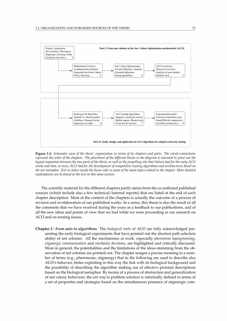
1.2 ORGANIZATION AND PUBLISHED SOURCES OF THE THESIS 11
3
Mathematical context:
Sequential decisions, States,Combinatorial problems,
Policy learning ...
Ant Colony Optimization:Formal definition, Analysis,Extended definition, Analysis of used models,
ACO in practice:Extensive overview,
Design guidelines ...
Nature’s inspiration:Ant Colonies, Pheromone,
Part I: From ants colonies to the Ant Colony Optimization metaheuristic (ACO)
Stigmergic learning, Paths,Stochastic decisions ...
Part II: Study, design, and application of ACO algorithms for adaptive network routing
Related work ...
2
4 5
Routing in IP Networks:
LinkState, DistanceVector,Adaptivity to traffic ...
Optimal vs. Shortest paths,ACO routing algorithms:Adaptive routing & control,Mobile agents, MonteCarlo,Proactive & reactive ... 8
Experimental results:Extensive simulation tests, StateOfTheArt competitors,Excellent performance ...6 7
Figure 1.1: Schematic view of the thesis’ organization in terms of its chapters and parts. The wired connectionsrepresent the order of the chapters. The placement of the different blocks in the diagram is intended to point out thelogical separation between the two parts of the thesis, as well as the propelling role that Nature had for the early ACOworks and that, in turn, ACO had for the development of competitive routing algorithms and architectures based onthe ant metaphor. Text in italics inside the boxes refer to some of the main topics related to the chapter. More detailedexplanations can be found in the text in this same section.
The scientific material for the different chapters partly stems from the co-authored published
sources (which include also a few technical/internal reports) that are listed at the end of each
chapter description. Most of the content of the chapters is actually the outcome of a process of
revision and re-elaboration of our published works. In a sense, this thesis is also the result of all
the comments that we have received during the years as a feedback to our publications, and of
all the new ideas and points of view that we had while we were proceeding in our research on
ACO and on routing issues.
Chapter 2 - From ants to algorithms. The biological roots of ACO are fully acknowledged pre-
senting the early biological experiments that have pointed out the shortest path selection
ability of ant colonies. All the mechanisms at work, especially pheromone laying/sensing,
stigmergic communication and stochastic decisions, are highlighted and critically discussed.
More in general, the potentialities and the limitations of the ideas stemming from the ob-
servation of ant colonies are pointed out. The chapter assigns a precise meaning to a num-
ber of terms (e.g., pheromone, stigmergy) that in the following are used to describe also
ACO’s behavior, better exploiting in this way the link with its biological background and
the possibility of describing the algorithm making use of effective pictorial descriptions
based on the biological metaphor. By means of a process of abstraction and generalization
of ant colony behaviors, the ant-way to problem solution is informally defined in terms of
a set of properties and strategies based on the simultaneous presence of stigmergic com-
12 1. INTRODUCTION
munication protocols and stigmergic variables that prime the response of a number of
relatively simple and concurrent agents.
This chapter is a revised and substantial extension of the content of the journal paper [147]
where ACO was first defined.
Published sources: [147]
Chapter 3 - Combinatorial optimization, construction methods, and decision processes. Before
providing in Chapter 4 the formal definition of the ACO metaheuristic, in Chapter 3 we
provide the formal tools and the basic scientific background that are going to be used at
the time ACO is defined and discussed. Here we define/introduce those mathematical
notions and terms that are useful if not necessary to reason about ACO. In turn, with these
notions in the hands, we point out few other general frameworks that we see as directly
related to ACO and from which we import some basic results, ideas, and models.
The content of the chapter can be also seen as a sort of high-level “related work”, although
discussions on related approaches are practically spread all over the thesis. Amore focused
discussion in this sense is given in Chapter 5, and some general discussions can also be
found in Chapter 4.
The topics considered in this chapter result from the specific way ACO is seen in this the-
sis, that is, in the terms of a multi-agent metaheuristic featuring solution construction, use
of memory, repeated solution sampling, and learning of the parameters of the construc-
tion policy over a small subspace. The chapter goes through all these and related issues:
(i) first, the characteristics of the combinatorial optimization problems addressed by ACO
are defined, (ii) then the issue of problem representation is considered, (iii) according to the
fact that, mimicking real ants, each ant-like agent generates a solution according to an in-
cremental step-by-step approach, the class of construction heuristics is defined, (iv) solution
construction can be conveniently seen in the more general terms of a sequential decision
process, therefore, the framework of sequential decision processes is introduced, stressing
the notion of process state (corresponding to a partial solution) and its relationships with
the fields of control [47], dynamic programming [20, 23], and Markov decision processes [353],
(v) then, the chapter introduces the graphical tools (like state and construction graphs) that
can be used to reason on and represent the structure and the dynamics of construction
processes, (vi) the notion of phantasma is defined, to indicate a subset or a feature of the
complete information state of the decision process, and which correspond to pheromone
variables, (vii) finally, some of the different general approaches to combinatorial optimiza-
tion, in particular those using or not states and state-value functions (e.g., dynamic pro-
gramming) are discussed, stressing the relative differences in terms of used information
and expected finite-time performance.
The originality of this chapter consists in the fact that it brings together in a coherent way
several notions from different fields. Most of its content comes from critical literature re-
view. However, part of the ideas, as well as the link between ACO and control / dynamic
programming, come from the two references below (one technical report [33] and one con-
ference paper [34]) were ant programming was introduced as a framework which presents
most of the characterizing features of ACO but which is more amenable to theoretical anal-
ysis and bridges the terminological gap between ACO and the fields of control [23] and re-
inforcement learning [414]. The work on ant programming has given a major contribution
to the way ACO is seen in this thesis.
Published sources: [34, 33]
Chapter 4 - The Ant Colony Optimization Metaheuristic (ACO). In this chapter ACO is formally
defined and its characteristics are throughly discussed by exploiting the notions and the
1.2 ORGANIZATION AND PUBLISHED SOURCES OF THE THESIS 13
terminology introduced in the previous chapter. The ACO’s definition is given in two
steps. In the first step, ACO is defined in a way which is fully compliant with the original
definition given by Dorigo and Di Caro (1999) in [138] but adopting a slightly different,
more precise, terminology. In the second step, the definition is revised and extended in
order to be able to account for all those algorithms designed (after 1999) according to the
general ACO’s ideas but which formally could not completely fit into the original ACO
definition. This is the case of several implementations for scheduling, set and constraint
satisfaction problems. This process of revision of the definition is in a sense in fully accor-
dance with the nature of ACO as an a posteriori synthesis. The revision of the definition
goes in the direction of generalizing both the characteristics of the state information which
is retained for the purpose of learning and optimization, and the way this information
is combined and used at decision time. In the original definition only the last compo-
nent included in the solution and single pheromone variables were considered at decision
time. The new definition overcomes these limitations providing the possibility of using the
amount of information which is judged as the most appropriate given the characteristics
of the optimization task at hand.
The definition of ACO is given by making a clear distinction among the different de-
sign steps, consisting in the definition of: (i) the problem representation and the phero-
mone model, (ii) the construction strategy adopted by an ant, and (iii) the strategies for
pheromone updating and ant generation. All these steps are described in detail. Following
the definition, an extensive discussion on the general characteristics of ACO is reported,
and in particular on the role played by the pheromone model, the use of memory and
learning, the use of stochastic components, the different strategies for pheromone updat-
ing, and so on.
Definitions and analysis of the ACO metaheuristic have been published in one journal
paper [147], one book chapter [138], and one conference paper [137]. The revised and
extended definitions have not been published yet, but find their roots in the previously
mentioned work on ant programming.
Published sources: [138, 147, 137, 34, 33]
Chapter 5 - Application of ACO to combinatorial optimization problems. In this chapter most
of the ACO implementations are reviewed on a per problem basis, with the purpose of
providing a complete picture of the different combinatorial problems that have been at-
tacked so far and of the design solutions that have been proposed, particularly in terms of
pheromone models and stochastic decision rules. ACO applications in the field of telecom-
munication networks are only listed but not reviewed, since this is done in Chapter 7. On
the other hand, applications in all the other domains of application, as well as parallel
models and implementations, are reviewed in detail.
In addition, the chapter reports a discussion on ACO related work, mainly focusing on those
approaches for combinatorial optimization that make use of stochastic components, pa-
rameter learning, population of solutions, and so on (e.g., evolutionary algorithms [202,
172], distribution estimation algorithms [329, 266], rollout algorithms [28], cultural algo-
rithms [366, 86]).
The chapter is concluded by a Summary that opens the way to the second part of the the-
sis, where the application of ACO to problems of adaptive routing in telecommunication
networks is considered. In the Summary the domain of dynamic network problems is
identified as the most appropriate for ACO characteristics. That is, as the application do-
main in which ACO characteristics can be fully exploited and ACO design guidelines can
naturally result in truly innovative and extremely effective control algorithms.
14 1. INTRODUCTION
The chapter is the result of extensive literature review of ACO implementations and of re-
lated frameworks. Part of the material comes from the previously mentioned publications
on ACO, that, however, cover only implementations and part of the related work up to
1999. Other important sources for this chapter have been the activities of co-editor of a
journal special issue [149] and of a conference proceedings book [150].
Published sources: [138, 147, 149, 150, 113]
Chapter 6 - Routing in telecommunication networks. This first chapter of the second part pro-
vides a general overview on routing in telecommunication networks. This chapter (which
is complemented by Appendix F that describes the different criteria to classify a network)
has been compiled for the sake of completeness for the reader not fully acquainted with
telecommunication issues, as well as to point out where the critical problems are and
which are the general directions to follow in order to optimize the performance of routing
strategies (i.e., to go in the direction of so-called traffic engineering [9], which is receiving a
tremendous attention in recent times by the Internet community).
The chapter defines the characteristics of the problem of routing in wired IP networks (e.g.,
the Internet), which is the class of routing problemsmost considered in this thesis (and also
the most pervasive one), and provides a description of both static and adaptive routing al-
gorithms that have been designed for this class of problems. The chapter also discusses
the metrics for performance evaluation and the reasons that make routing a particularly
hard problem to deal with. The characteristics of, and the relationships between, the most
popular routing paradigms, optimal [26] and shortest path routing [398, 441, 387], are dis-
cussed. For the shortest path case, the characteristics of popular link-state and distance-
vector architectures are thoroughly analyzed in order to get a precise understanding of the
pro and cons of these approaches which cover the majority of current routing implemen-
tations. The conclusion is that there is still much space for improvements when adaptivity
to traffic patterns is considered.
The full content of the chapter is the result of an extensive work of literature review and
analysis which was partly already included in the DEA thesis [113] and in the AntNet’s
journal paper [120].
Published sources: [120, 113]
Chapter 7 - ACO algorithms for adaptive routing. In this chapter four ACO algorithms for adap-
tive routing tasks in telecommunication networks are introduced and their general char-
acteristics are discussed and compared to those of the most used routing approaches. In
particular, the chapter introduces AntNet, AntNet-FA, AntNet+SELA, and AntHocNet. The
four algorithms cover a complete spectrum of networks and delivered services. In fact,
AntNet and AntNet-FA are designed for best-effort routing in wired datagram networks,
AntHocNet is for best-effort routing in mobile ad hoc networks, and AntNet+SELA is in-
tended for QoS routing in ATM networks. In addition to these four algorithms, the chap-
ter also introduces Ant Colony Routing (ACR), a general framework for adaptive control in
networks which extends and generalizes ACO ideas by making use of both learning and
ant-like agents.
AntNet stems directly from the ACO’s general ideas adapted to the specificities of network
environments, and is intended to providemulti-path traffic-adaptive routing in best-effort IP
wired networks. It features mobile autonomous agents that proactively sample paths connect-
ing node pairs, use of probabilistic routing tables directly derived from tables of pheromone
variables for both the ant-like agents and data packets, use of local statistical models to
adaptively score the quality of the sampled paths and to update pheromone tables, etc.
AntNet realizes in a robust way active information gathering in the form of repeated sam-
1.2 ORGANIZATION AND PUBLISHED SOURCES OF THE THESIS 15
pling of full paths, while most of the other routing algorithms, as well as algorithms for
other network tasks (e.g., performance monitoring), implement only passive information
gathering. More in general, several of the AntNet’s characteristics represents a departure
from more “classical” routing algorithms.
AntNet-FA consists in a little modification over AntNet (ants move only over high-priority
queues and their end-to-end delays are estimated according to statistical models depend-
ing on local link queues). Nevertheless, the AntNet-FA’s performance is always similar or
better than that of AntNet, and the relative performance improves as the network size gets
larger.
AntHocNet and AntNet+SELA are introduced for the double purpose of covering the full
spectrum of the most challenging routing problems and as practical examples of the ACR’s
ideas. Nevertheless, they are explained with less detail than AntNet and AntNet-FA, and
experimental results will be reported only for AntHocNet.5
AntNet+SELA is a model for delivering both best-effort and QoS (e.g., [440, 79, 208]) traffic
in ATM (connection-oriented) networks. It is a hybrid algorithm that combines AntNet-
FA with a stochastic estimator learning automaton [430] at the nodes. In addition to same
best-effort functionalities that have in AntNet-FA, the ant-like agents serve for the purpose
of gathering information which is exploited by the automata to define and allocate on-
demand feasible paths for the QoS traffic sessions.
AntHocNet is a traffic- and topology-adaptive algorithm for best-effort multipath routing
in mobile ad hoc networks (e.g., [399, 61]). In addition to the components common also to
the other algorithms and that directly derive from ACO, AntHocNet features: on-demand
generation of ant agents to find paths toward those destinations that are required by a
traffic session and for which no routing information is maintained at the node, continual
cleanup of obsolete routing information, proactive ant generation on a pure per-session
basis for path maintenance and improvement, local repair of link failures, and so on.
ACR is a general framework of reference and a collection of ideas/strategies for the design
of autonomic routing systems [250]. It defines the generalities of a multi-agent society based
on the integration of the ACO’s philosophy and ideas from the domain of reinforcement
learning [414, 27]. The aim is to provide a meta-architecture of reference for the design
and implementation of fully adaptive and distributed routing/control systems that can
be applied to a wide range of network scenarios. The formalization of ACR is still at a
preliminary stage, however, all the necessary building blocks of fully autonomic systems
are already introduced.
The chapter includes also a review of current AntNet-inspired and, more generally, ant-
based implementations for routing tasks.
The content of this chapter is derived from one journal publication [120] (actually, two,
since another journal [125] asked the permission to re-publish the paper), six publica-
tions in conference proceedings [128, 124, 122, 121, 119, 115], and other sources (DEA
thesis [113], conferences with only abstract proceedings [118, 126], internal and techni-
cal reports [115, 127, 129], on going work [155, 130]).
Published sources: [120, 125, 122, 124, 121, 119, 115, 116, 113, 118, 126, 127, 128, 155, 130, 129]
5 The reasons are of practical order. First, to be able to appreciate the details of the algorithms, an extensive reviewof technical issues related to QoS, ATM, and mobile ad hoc networks would have been necessary. Such a review wouldhave made this thesis unnecessarily too long. Second, the implementation of AntNet+SELA has not been fully testedand debugged, such that it is not possible to report experimental results about it. On the other hand, AntHocNet is stillunder intensive development and improvement (see also Footnote 4).
16 1. INTRODUCTION
Chapter 8 - Experimental results for ACO algorithms for routing. In this chapter, experimental
results obtained by simulation are reported for AntNet, AntNet-FA, and AntHocNet.
According to extensive simulation studies of a wide range of situations in terms of different
networks (ranging from 8 to 150 nodes) and traffic patterns, both AntNet and AntNet-
FA clearly outperform a set of five state-of-the-art routing algorithms. On the other side,
AntHocNet is compared to AODV [349, 103], a popular state-of-the-art algorithm, over a
range of scenarios up to 2000 nodes and with different number of nodes, node density, and
mobility. AntHocNet’s performance is always better or comparable than that of AODV,
with AntHocNet performing relatively better in the most challenging scenarios.
The results and the rationale behind them are throughly discussed, validating the view that
the design characteristics of ACO are particularly suited for the characteristics of network
problems and can be considered as a valid alternative to more established approaches.
Material from this chapter comes from the same sources cited for the previous chapter.
Published sources: The same of Chapter 7
Chapter 9 - Summary and Future work. The results presented across the thesis are summarized
and all the major scientific contributions are pointed out. Some general conclusions are
drawn and ideas for future possible works are also listed.
Appendices. Several appendices are included at the end of the thesis. They have been included
for sake of completeness and clarity. Some of the appendices have the purpose of only
briefly discussing general and consolidated issues. This is the case of: (i) Appendix A,
which provides definitions for most of the combinatorial problems mentioned in the text,
so these problems do not need to be defined in the text, (ii) Appendix C, which discusses
the generalities of observable and partially observable Markov decision processes, (iii) Ap-
pendix E, that gives a very short and informal definition and discussion of reinforcement
learning, and (iv) Appendix D that informally discusses Monte Carlo methods, and points
out what we precisely mean here with this term (we use it here with the same meaning
it has in the field of reinforcement learning). Appendix B could have found its place in
the main text, since it introduces original definitions for the class of modification methods
(seen as complementary to construction methods) and discusses their general properties.
However, we have chosen to move these discussions in the appendices since they are seen
as a sort of “extras”. Appendix F has already been mentioned: it provides an overview on
the different types of networks and complements the content of Chapter 6.
Examples and Summaries. A final note on the use of examples and summaries. Across the
thesis we have made an extensive use of examples to explain concepts, consider specific
cases, suggest new ideas, and, in general, to discuss issues that a practical example can
make immediately clear while otherwise a more general and rigorous explanation would
have required a lengthy discussion. In many cases examples can be skippedwithout losing
continuity, but likely losing some interesting bit of information or ideas.
Each chapter is ended by a Summary section whose role is twofold. From one side, it
provides a brief summary of the contents of the chapter in order to provide a unified view
of themost important topics that have been just discussed. On the other side, the Summary
represents the place where important conclusions are drawn from the contents discussed
in the chapter and the topics that are going to be discusses in the chapter that follows are
introduced.
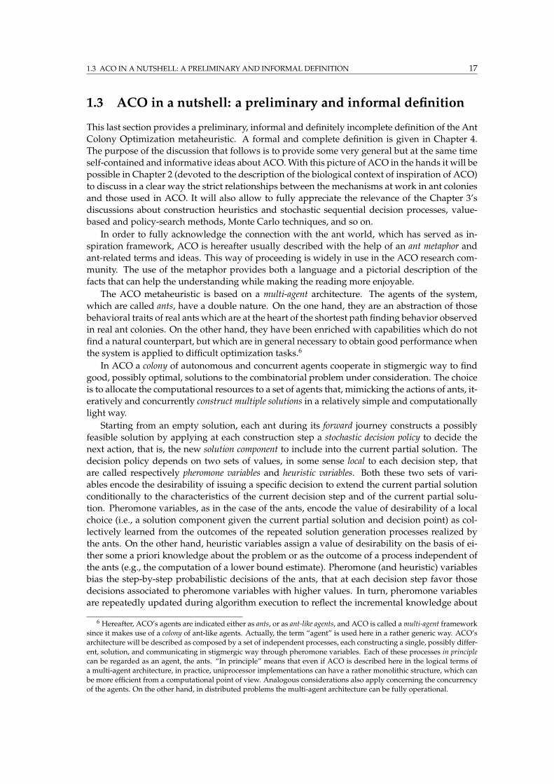
1.3 ACO IN A NUTSHELL: A PRELIMINARY AND INFORMAL DEFINITION 17
1.3 ACO in a nutshell: a preliminary and informal definition
This last section provides a preliminary, informal and definitely incomplete definition of the Ant
Colony Optimization metaheuristic. A formal and complete definition is given in Chapter 4.
The purpose of the discussion that follows is to provide some very general but at the same time
self-contained and informative ideas about ACO.With this picture of ACO in the hands it will be
possible in Chapter 2 (devoted to the description of the biological context of inspiration of ACO)
to discuss in a clear way the strict relationships between the mechanisms at work in ant colonies
and those used in ACO. It will also allow to fully appreciate the relevance of the Chapter 3’s
discussions about construction heuristics and stochastic sequential decision processes, value-
based and policy-search methods, Monte Carlo techniques, and so on.
In order to fully acknowledge the connection with the ant world, which has served as in-
spiration framework, ACO is hereafter usually described with the help of an ant metaphor and
ant-related terms and ideas. This way of proceeding is widely in use in the ACO research com-
munity. The use of the metaphor provides both a language and a pictorial description of the
facts that can help the understanding while making the reading more enjoyable.
The ACO metaheuristic is based on a multi-agent architecture. The agents of the system,
which are called ants, have a double nature. On the one hand, they are an abstraction of those
behavioral traits of real ants which are at the heart of the shortest path finding behavior observed
in real ant colonies. On the other hand, they have been enriched with capabilities which do not
find a natural counterpart, but which are in general necessary to obtain good performance when
the system is applied to difficult optimization tasks.6
In ACO a colony of autonomous and concurrent agents cooperate in stigmergic way to find
good, possibly optimal, solutions to the combinatorial problem under consideration. The choice
is to allocate the computational resources to a set of agents that, mimicking the actions of ants, it-
eratively and concurrently construct multiple solutions in a relatively simple and computationally
light way.
Starting from an empty solution, each ant during its forward journey constructs a possibly
feasible solution by applying at each construction step a stochastic decision policy to decide the
next action, that is, the new solution component to include into the current partial solution. The
decision policy depends on two sets of values, in some sense local to each decision step, that
are called respectively pheromone variables and heuristic variables. Both these two sets of vari-
ables encode the desirability of issuing a specific decision to extend the current partial solution
conditionally to the characteristics of the current decision step and of the current partial solu-
tion. Pheromone variables, as in the case of the ants, encode the value of desirability of a local
choice (i.e., a solution component given the current partial solution and decision point) as col-
lectively learned from the outcomes of the repeated solution generation processes realized by
the ants. On the other hand, heuristic variables assign a value of desirability on the basis of ei-
ther some a priori knowledge about the problem or as the outcome of a process independent of
the ants (e.g., the computation of a lower bound estimate). Pheromone (and heuristic) variables
bias the step-by-step probabilistic decisions of the ants, that at each decision step favor those
decisions associated to pheromone variables with higher values. In turn, pheromone variables
are repeatedly updated during algorithm execution to reflect the incremental knowledge about
6 Hereafter, ACO’s agents are indicated either as ants, or as ant-like agents, and ACO is called amulti-agent frameworksince it makes use of a colony of ant-like agents. Actually, the term “agent” is used here in a rather generic way. ACO’sarchitecture will be described as composed by a set of independent processes, each constructing a single, possibly differ-ent, solution, and communicating in stigmergic way through pheromone variables. Each of these processes in principlecan be regarded as an agent, the ants. “In principle” means that even if ACO is described here in the logical terms ofa multi-agent architecture, in practice, uniprocessor implementations can have a rather monolithic structure, which canbe more efficient from a computational point of view. Analogous considerations also apply concerning the concurrencyof the agents. On the other hand, in distributed problems the multi-agent architecture can be fully operational.

18 1. INTRODUCTION
the characteristics of the solution set that has been acquired through the iterative generation of
multiple solutions.
In particular, after building a solution, the ant metaphorically reports the solution to a phero-
mone manager, which authorizes or not the ant to update the pheromone variables associated
to the built solution. In the positive case, the ant starts its backward journey, retracing its solu-
tion and updating pheromone values, usually of an amount proportional to the quality of the
solution. In this way, decisions associated to solutions which are either of good quality or are
chosen more often, will likely have associated higher levels of pheromone, that is, higher local
desirability. In most of the cases when centralized implementations are possible, the retracing
is purely metaphoric, but in the case of fully distributed problems, like routing in communica-
tion networks, the ant agent physically retraces backward the network nodes visited during its
forward journey. Another peculiar characteristics of network problems consists in the fact that
a proper evaluation of the quality of a solution (e.g., a path joining a (source,destination) pair of
network nodes) is often rather hard to obtain because of the distributed and dynamic nature of
the problem. For instance, because of the continually changing traffic patterns, the same locally
observed value of end-to-end delay can be a good one or a bad one depending on the overall sta-
tus of network congestion. Unfortunately, a correct and up-to-date view of this status cannot be
locally accessed in real-time. On the other hand, in the case of non-dynamic and non-distributed
problems, it is usually rather easy to provide a proper solution evaluation.
The complexity of each ant-like agent is such that it can quickly build a feasible solution, but
high quality solutions are expected to be the overall result of the accumulation and exchange of
information among the agents during the whole execution time of the algorithm. In the same
spirit of ants in Nature, the set of capabilities in the repertoire of the single agent is purposely
minimal: the agent’s complexity is such that according to the allocated time and resources a
relatively large number of solutions can be generated. Moreover, the agent is in general not sup-
posed to be adaptive or to learn during its lifetime (in fact, after generating a solution an ant is
usually removed from the colony). On the contrary, learning is expected to happen at a collec-
tive level through repeated solution sampling and collective/stigmergic exchange of information
about the sampled solutions.
Algorithm 1.1 shows in C-like pseudo-code the very general structure of the ACO meta-
heuristic. The algorithm is organized in three main logical blocks. Ant-like agents generate
solutions through incremental construction processes governed by a stochastic decision pol-
icy. In turn, the decision policy depends on the value of pheromone variables which are in
a sense that is explained in the following chapters local to each step of the construction pro-
cess (ants construct solutions using pheromone() block). The generated solutions are
used, in turn, to update the pheromone variables themselves, in the attempt to bias the whole
generation process towards those regions of the solution space where the best solutions are
expected to be found. The processes in the pheromone updating() block manage all the
activities concerning updating of pheromone variables, like: authorize/deny ants to update
pheromone, decrease the pheromone levels bymimicking natural evaporation processes in order
to favor exploration, update pheromone according to communications coming from the daemon
block (see below). This logical block of strictly pheromone-related activities is also indicated
in the following as pheromone manager. The ACO metaheuristic proceeds iteratively, by a con-
tinual generation of solutions and the updating of the parameters of the decision policy used
to construct the solutions themselves. The generation of solutions, as well as the updating of
the pheromones, can be realized according to either distributed or centralized, concurrent or
sequential schemes, depending on the characteristics of the problem and of the design of the
specific implementation. The construct schedule activities summarizes all these possibil-
ities. The block termed daemon actions() refers to all those optional activities which share
no relationship with the biological context of inspiration of the metaheuristic and which, at the
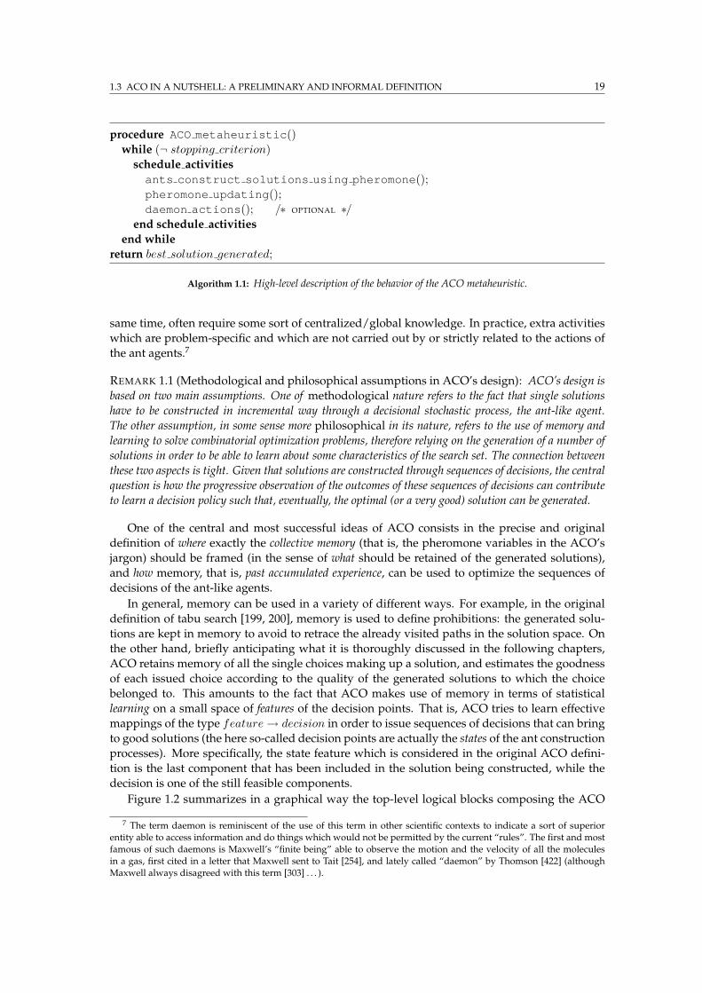
1.3 ACO IN A NUTSHELL: A PRELIMINARY AND INFORMAL DEFINITION 19
procedure ACO metaheuristic()
while (¬ stopping criterion)
schedule activities
ants construct solutions using pheromone();
pheromone updating();
daemon actions(); /∗ OPTIONAL ∗/end schedule activities
end while
return best solution generated;
Algorithm 1.1: High-level description of the behavior of the ACO metaheuristic.
same time, often require some sort of centralized/global knowledge. In practice, extra activities
which are problem-specific and which are not carried out by or strictly related to the actions of
the ant agents.7
REMARK 1.1 (Methodological and philosophical assumptions in ACO’s design): ACO’s design is
based on two main assumptions. One of methodological nature refers to the fact that single solutions
have to be constructed in incremental way through a decisional stochastic process, the ant-like agent.
The other assumption, in some sense more philosophical in its nature, refers to the use of memory and
learning to solve combinatorial optimization problems, therefore relying on the generation of a number of
solutions in order to be able to learn about some characteristics of the search set. The connection between
these two aspects is tight. Given that solutions are constructed through sequences of decisions, the central
question is how the progressive observation of the outcomes of these sequences of decisions can contribute
to learn a decision policy such that, eventually, the optimal (or a very good) solution can be generated.
One of the central and most successful ideas of ACO consists in the precise and original
definition of where exactly the collective memory (that is, the pheromone variables in the ACO’s
jargon) should be framed (in the sense of what should be retained of the generated solutions),
and how memory, that is, past accumulated experience, can be used to optimize the sequences of
decisions of the ant-like agents.
In general, memory can be used in a variety of different ways. For example, in the original
definition of tabu search [199, 200], memory is used to define prohibitions: the generated solu-
tions are kept in memory to avoid to retrace the already visited paths in the solution space. On
the other hand, briefly anticipating what it is thoroughly discussed in the following chapters,
ACO retains memory of all the single choices making up a solution, and estimates the goodness
of each issued choice according to the quality of the generated solutions to which the choice
belonged to. This amounts to the fact that ACO makes use of memory in terms of statistical
learning on a small space of features of the decision points. That is, ACO tries to learn effective
mappings of the type feature→ decision in order to issue sequences of decisions that can bring
to good solutions (the here so-called decision points are actually the states of the ant construction
processes). More specifically, the state feature which is considered in the original ACO defini-
tion is the last component that has been included in the solution being constructed, while the
decision is one of the still feasible components.
Figure 1.2 summarizes in a graphical way the top-level logical blocks composing the ACO
7 The term daemon is reminiscent of the use of this term in other scientific contexts to indicate a sort of superiorentity able to access information and do things which would not be permitted by the current “rules”. The first and mostfamous of such daemons is Maxwell’s “finite being” able to observe the motion and the velocity of all the moleculesin a gas, first cited in a letter that Maxwell sent to Tait [254], and lately called “daemon” by Thomson [422] (althoughMaxwell always disagreed with this term [303] . . . ).
20 1. INTRODUCTION
metaheuristic and their relationships. The central role ofmemory, that is, of the use of pheromone
variables, is stressed by positioning the pheromone manager in the middle of the diagram and
by differentiating the ant from the daemon processes precisely according to the use or not of
pheromone.
Problem Representation
ManagerPheromone
Decision Points
Pheromone
Schedule Activities
Using Pheromone
Ant-like agents
Daemon actions
of Solutions
Incremental Construction
Pheromone
Generation of Solutions
Combinatorial Problem
Without the Use of
Figure 1.2: The logical blocks composing the ACO metaheuristic and their mutual interactions. The daemon’scircular diagram is dotted to express the optional characteristic of such a component. The diagram labeled “problemrepresentation” summarizes the transformation that ACO operates on the original formulation of the combinatorialproblem in order to generate solutions by incremental construction and to make use of some form of memory of thegenerated solutions in the pheromones variables. The presence of an arrow indicates the existence of an interactionbetween the blocks, while the arrow’s direction represents the direction of the main information flows.
Part I
From real ant colonies to the
Ant Colony Optimization
metaheuristic

CHAPTER 2
Ant colonies, the biological roots of
Ant Colony Optimization
The aim of this chapter is to acknowledge the fundamental role provided by Nature’s inspira-
tion in the design of ACO. The following pages describe and informally discuss the biological
experiments that showed how and under which conditions ant colonies can select shortest paths.
These experiments provided, at the beginning of the 1990s [135, 144, 91], the first impetus to the
design of Ant Colony Optimization algorithms.
The chapter singles out all the principal ingredients participating to the shortest path be-
havior (e.g., path construction, pheromone and pheromone-biased stochastic decisions), and discusses
the properties of the system resulting from their combination and interaction. In particular, the
limits of the approach are pointed out, as well as its characteristics of robustness, adaptivity, and
self-organization. In the perspective using ant colonies as a source of inspiration for the design of
distributed multi-agent systems possessing these same appealing properties, we will point out few
nonlinear dynamics that are at the very core of the ant colony behaviors and that are the direct
responsible for these properties (not only in ant colonies, but likely in all societal organizations).
These dynamics are explained using the notion of stigmergy, that expresses the general idea of
using indirect communication mediated by physical modifications of the environment (in the
form of so-called stigmergic variables) to activate and coordinate self-organized behaviors in a
colony of insects, or, more in general, in a set of autonomous agents. From the notion of stig-
mergy we define the notion of stigmergic design, that is, system design focusing on the protocols
of interaction among a number of “cheap” (relatively simple) agents, rather than on the design
of “expensive”/complex modules with little or no interaction at all.
The ultimate goal of the cross-disciplinary discussions reported in the chapter consists in
showing the rationale, the advantages, and the potential problems behind the choice of taking
ant colony behaviors (or, more in general, insect society behaviors) as a reference to guide the
design of multi-agent systems, as it has happened in the case of the ACO metaheuristic.
Organization of the chapter
Section 2.1 describes and discusses the experimental results showing how ant colonies can se-
lect the shortest among few possible alternative paths connecting their nest to food reservoirs.
The following Section 2.2 points out all the elements concurring to the shortest path behavior, as
well as potential problems and intrinsic limitations. Section 2.3 discusses the general properties
of adaptivity and self-organization in ant colonies, and, more in general, in insect societies. The
conclusive Section 2.4 defines stigmergy as an effective way to capture and represent the nonlin-
ear dynamics at the very core of ant colonies’ behaviors. The characteristics of stigmergy-based
design of multi-agent systems are discussed, and the “ant way” to problem-solving is also infor-
mally defined.
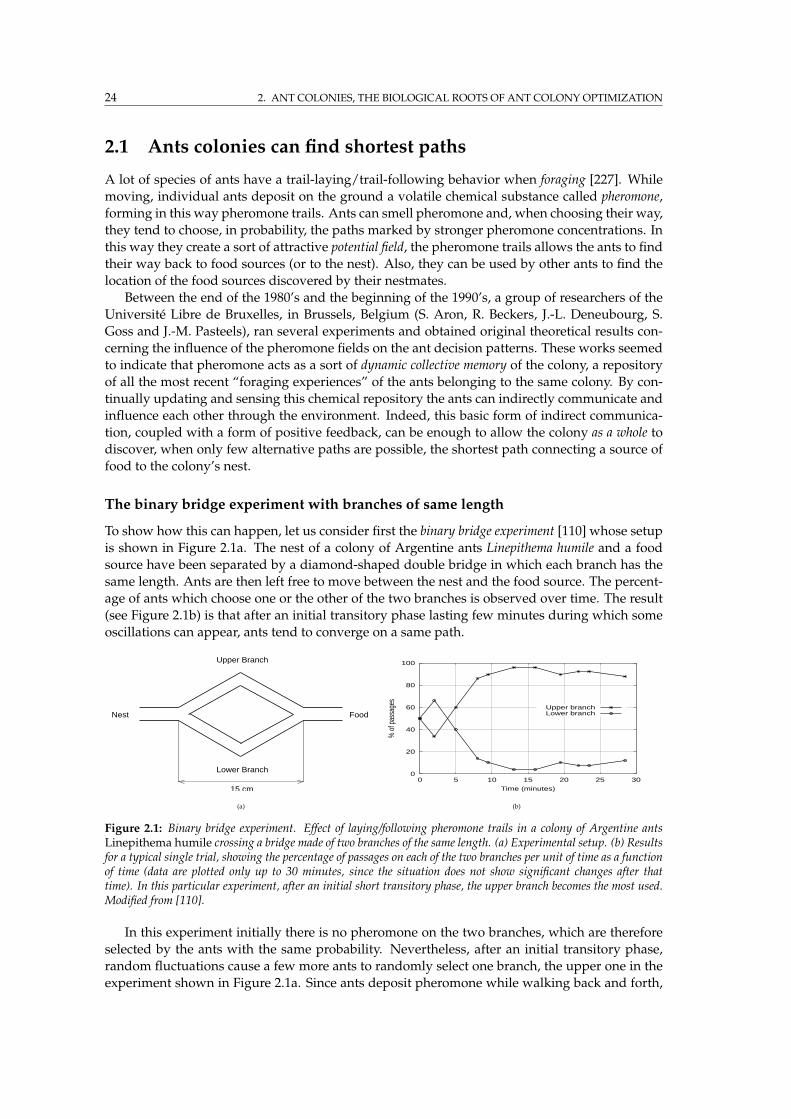
24 2. ANT COLONIES, THE BIOLOGICAL ROOTS OF ANT COLONY OPTIMIZATION
2.1 Ants colonies can find shortest paths
A lot of species of ants have a trail-laying/trail-following behavior when foraging [227]. While
moving, individual ants deposit on the ground a volatile chemical substance called pheromone,
forming in this way pheromone trails. Ants can smell pheromone and, when choosing their way,
they tend to choose, in probability, the paths marked by stronger pheromone concentrations. In
this way they create a sort of attractive potential field, the pheromone trails allows the ants to find
their way back to food sources (or to the nest). Also, they can be used by other ants to find the
location of the food sources discovered by their nestmates.
Between the end of the 1980’s and the beginning of the 1990’s, a group of researchers of the
Universite Libre de Bruxelles, in Brussels, Belgium (S. Aron, R. Beckers, J.-L. Deneubourg, S.
Goss and J.-M. Pasteels), ran several experiments and obtained original theoretical results con-
cerning the influence of the pheromone fields on the ant decision patterns. These works seemed
to indicate that pheromone acts as a sort of dynamic collective memory of the colony, a repository
of all the most recent “foraging experiences” of the ants belonging to the same colony. By con-
tinually updating and sensing this chemical repository the ants can indirectly communicate and
influence each other through the environment. Indeed, this basic form of indirect communica-
tion, coupled with a form of positive feedback, can be enough to allow the colony as a whole to
discover, when only few alternative paths are possible, the shortest path connecting a source of
food to the colony’s nest.
The binary bridge experiment with branches of same length
To show how this can happen, let us consider first the binary bridge experiment [110] whose setup
is shown in Figure 2.1a. The nest of a colony of Argentine ants Linepithema humile and a food
source have been separated by a diamond-shaped double bridge in which each branch has the
same length. Ants are then left free to move between the nest and the food source. The percent-
age of ants which choose one or the other of the two branches is observed over time. The result
(see Figure 2.1b) is that after an initial transitory phase lasting few minutes during which some
oscillations can appear, ants tend to converge on a same path.
Upper Branch
Nest Food
15 cm
Lower Branch
(a)
0
20
40
60
80
100
0 5 10 15 20 25 30
% o
f pas
sage
s
Time (minutes)
Upper branchLower branch
(b)
Figure 2.1: Binary bridge experiment. Effect of laying/following pheromone trails in a colony of Argentine antsLinepithema humile crossing a bridge made of two branches of the same length. (a) Experimental setup. (b) Resultsfor a typical single trial, showing the percentage of passages on each of the two branches per unit of time as a functionof time (data are plotted only up to 30 minutes, since the situation does not show significant changes after thattime). In this particular experiment, after an initial short transitory phase, the upper branch becomes the most used.Modified from [110].
In this experiment initially there is no pheromone on the two branches, which are therefore
selected by the ants with the same probability. Nevertheless, after an initial transitory phase,
random fluctuations cause a few more ants to randomly select one branch, the upper one in the
experiment shown in Figure 2.1a. Since ants deposit pheromone while walking back and forth,
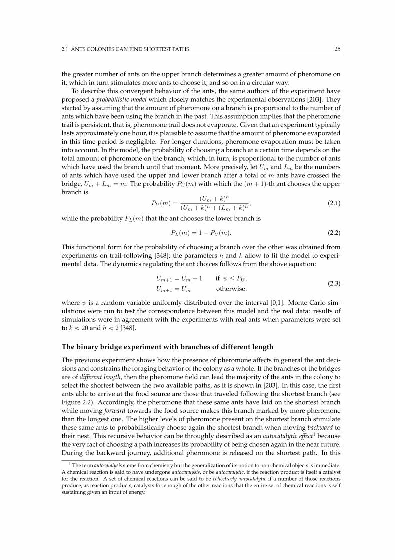
2.1 ANTS COLONIES CAN FIND SHORTEST PATHS 25
the greater number of ants on the upper branch determines a greater amount of pheromone on
it, which in turn stimulates more ants to choose it, and so on in a circular way.
To describe this convergent behavior of the ants, the same authors of the experiment have
proposed a probabilistic model which closely matches the experimental observations [203]. They
started by assuming that the amount of pheromone on a branch is proportional to the number of
ants which have been using the branch in the past. This assumption implies that the pheromone
trail is persistent, that is, pheromone trail does not evaporate. Given that an experiment typically
lasts approximately one hour, it is plausible to assume that the amount of pheromone evaporated
in this time period is negligible. For longer durations, pheromone evaporation must be taken
into account. In the model, the probability of choosing a branch at a certain time depends on the
total amount of pheromone on the branch, which, in turn, is proportional to the number of ants
which have used the branch until that moment. More precisely, let Um and Lm be the numbers
of ants which have used the upper and lower branch after a total of m ants have crossed the
bridge, Um + Lm = m. The probability PU (m) with which the (m+ 1)-th ant chooses the upper
branch is
PU (m) =(Um + k)h
(Um + k)h + (Lm + k)h, (2.1)
while the probability PL(m) that the ant chooses the lower branch is
PL(m) = 1− PU (m). (2.2)
This functional form for the probability of choosing a branch over the other was obtained from
experiments on trail-following [348]; the parameters h and k allow to fit the model to experi-
mental data. The dynamics regulating the ant choices follows from the above equation:
Um+1 = Um + 1 if ψ ≤ PU ,Um+1 = Um otherwise,
(2.3)
where ψ is a random variable uniformly distributed over the interval [0,1]. Monte Carlo sim-
ulations were run to test the correspondence between this model and the real data: results of
simulations were in agreement with the experiments with real ants when parameters were set
to k ≈ 20 and h ≈ 2 [348].
The binary bridge experiment with branches of different length
The previous experiment shows how the presence of pheromone affects in general the ant deci-
sions and constrains the foraging behavior of the colony as awhole. If the branches of the bridges
are of different length, then the pheromone field can lead the majority of the ants in the colony to
select the shortest between the two available paths, as it is shown in [203]. In this case, the first
ants able to arrive at the food source are those that traveled following the shortest branch (see
Figure 2.2). Accordingly, the pheromone that these same ants have laid on the shortest branch
while moving forward towards the food source makes this branch marked by more pheromone
than the longest one. The higher levels of pheromone present on the shortest branch stimulate
these same ants to probabilistically choose again the shortest branch when moving backward to
their nest. This recursive behavior can be throughly described as an autocatalytic effect1 because
the very fact of choosing a path increases its probability of being chosen again in the near future.
During the backward journey, additional pheromone is released on the shortest path. In this
1 The term autocatalysis stems from chemistry but the generalization of its notion to non chemical objects is immediate.A chemical reaction is said to have undergone autocatalysis, or be autocatalytic, if the reaction product is itself a catalystfor the reaction. A set of chemical reactions can be said to be collectively autocatalytic if a number of those reactionsproduce, as reaction products, catalysts for enough of the other reactions that the entire set of chemical reactions is selfsustaining given an input of energy.

26 2. ANT COLONIES, THE BIOLOGICAL ROOTS OF ANT COLONY OPTIMIZATION
way, pheromone is laid on the shortest branch at a higher rate than on the longest branch. This
reinforcement of the pheromone intensity on the shorter paths is the result of a form of implicit
path evaluation: the shorter paths are completed earlier than the longer ones, and therefore they
receive pheromone reinforcement more quickly. Therefore, for a same number of ants choosing
either the shortest or the longest branch at the beginning, since the pheromone on the shortest
branch is accumulated at a higher rate than on the longest one, the choice of the shortest branch
becomes more and more attractive for the subsequent ants at both the decision points. The ex-
perimental observation is that, after a transitory phase which can last a few minutes, most of
the ants use the shortest branch. It is also observed that the colony’s probability of selecting the
shortest path increases with the difference in length between the long and the short branches.
Food1 2
Nest
(a)
Food2
Nest1
(b)
0
50
100
0-20 20-40 40-60 60-80 80-100
% o
ver n e
xperim
ents
% of ants selecting the shorter branch
n=14, r=2
(c)
Figure 2.2: Experiment with a binary bridge whose branches have different length. Effect of laying/followingpheromone trails in a colony of Argentine ants Linepithema humile crossing the bridge. (a) Ants start explor-ing the bridge. The straight line distance between the decision points 1 and 2 is 12.5cm. (b) Eventually most of theants choose the shortest path. This situation happens already after about 8 minutes. (c) Distribution of the percentageof ants that selected the shorter branch over n = 14 experiments for the case of a bridge with the long branch r = 2times longer than the short one. The distribution refers to what happens after a transitory phase of about 10 minutes.Modified from [203].
In this experiment, the importance of initial random fluctuations is much reduced with re-
spect to the previous experiment. In Figure 2.2a-b are shown, together with the experimental
apparatus, the typical result of an experiment with a bridge with branches of different lengths.
Figure 2.2c shows the distribution of the results over n = 14 experiments for the case of a bridge
in which the length r of the longer branch is twice that of the shorter one.
EXAMPLE 2.1: EFFECT OF PHEROMONE LAYING/SENSING TO DETERMINE CONVERGENCE
Figure 2.3 shows in a schematic way how the effect of round-trip pheromone laying/sensing can easily
determine the convergence of all the ants on the shortest between two available paths.
At time t = 0 two ants leave the nest looking for food. According to the fact that no pheromone is present
on the terrain at the nest site, the ants select randomly the path to follow. One ant chooses the longest and
one the shortest path bringing to the food. After one time unit, the ant who chose the shortest path arrives
at the food reservoir. The other ant is still on its way. The intensity levels of the pheromone deposited on the
terrain are shown, where the intensity scale on the right says that a darker color means more pheromone.
Pheromone evaporation is considered as negligible according to the time duration of the experiment. The
ant already arrived at the food site must select the way to go back to the nest. According to the intensity
levels of the pheromone near the food site, the ant decides to go back by moving along the same path, but
in the opposite direction. Additional pheromone is therefore deposited on the shortest branch. At t = 2
the ant is back to the nest, while the other ant is still moving toward the food along the longest path. At
t = 3 another ant moves from the nest looking for food. Again, he/she selects the path according to the
pheromone levels and, therefore, it is biased toward the choice of the shortest path. It is easy to imagine
how the process iterates, bringing, in the end, the majority of the ants on the shortest path.
2.2 SHORTEST PATHS AS THE RESULT OF A SYNERGY OF INGREDIENTS 27
Nest
Food
Pheromone Intensity Scale
t = 2 t = 3
t = 1
Nest
Food
Nest
FoodFood
Nest
t = 0
Figure 2.3: Example of how the effect of laying/sensing pheromone during the forth and back journeys from the nestto food sources can easily determine the convergence of all the ants of the colony to the shortest between two availablepaths. The example is explained in the text.
2.2 Shortest paths and other collective behaviors as the result
of a synergy of ingredients
According to the discussed experiments, the remarkable ability of ant colonies in selecting the
shortest among the available paths can be precisely understood as the result of the synergistic
and concurrent presence of a number of ingredients:
• population (colony) of foraging ants,
• forward-backward path following
• pheromone laying and sensing,
• pheromone-biased stochastic decisions,
• autocatalysis,
• implicit path evaluation,
• iteration over time.
The agents, that is, the ants of the colony, act in a completely asynchronous, concurrent and dis-
tributed fashion. Each ant can be considered as autonomous, and the overall control is completely
distributed. In this perspective, the colony realizes a form of concurrent computation. Multiple
paths are repeatedly tried out back and forth and some information related to each followed
path is released on the environment, which acts as a shared distributed memory encoded in the
pheromone trails. In turn, the local content of this memory affects the stochastic decisions of the
ants, such that, when there is a significant difference in the lengths of the possible paths, implicit
path evaluation gets at work and, coupled with autocatalysis, results in a distributed and collec-
tive path optimization mechanism. Given enough time (depending on the number of ants, length
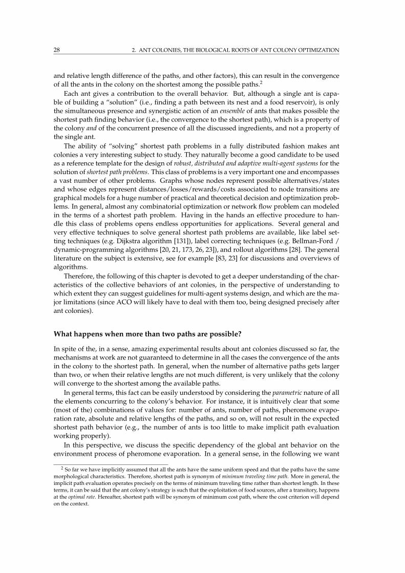
28 2. ANT COLONIES, THE BIOLOGICAL ROOTS OF ANT COLONY OPTIMIZATION
and relative length difference of the paths, and other factors), this can result in the convergence
of all the ants in the colony on the shortest among the possible paths.2
Each ant gives a contribution to the overall behavior. But, although a single ant is capa-
ble of building a “solution” (i.e., finding a path between its nest and a food reservoir), is only
the simultaneous presence and synergistic action of an ensemble of ants that makes possible the
shortest path finding behavior (i.e., the convergence to the shortest path), which is a property of
the colony and of the concurrent presence of all the discussed ingredients, and not a property of
the single ant.
The ability of “solving” shortest path problems in a fully distributed fashion makes ant
colonies a very interesting subject to study. They naturally become a good candidate to be used
as a reference template for the design of robust, distributed and adaptive multi-agent systems for the
solution of shortest path problems. This class of problems is a very important one and encompasses
a vast number of other problems. Graphs whose nodes represent possible alternatives/states
and whose edges represent distances/losses/rewards/costs associated to node transitions are
graphical models for a huge number of practical and theoretical decision and optimization prob-
lems. In general, almost any combinatorial optimization or network flow problem can modeled
in the terms of a shortest path problem. Having in the hands an effective procedure to han-
dle this class of problems opens endless opportunities for applications. Several general and
very effective techniques to solve general shortest path problems are available, like label set-
ting techniques (e.g. Dijkstra algorithm [131]), label correcting techniques (e.g. Bellman-Ford /
dynamic-programming algorithms [20, 21, 173, 26, 23]), and rollout algorithms [28]. The general
literature on the subject is extensive, see for example [83, 23] for discussions and overviews of
algorithms.
Therefore, the following of this chapter is devoted to get a deeper understanding of the char-
acteristics of the collective behaviors of ant colonies, in the perspective of understanding to
which extent they can suggest guidelines for multi-agent systems design, and which are the ma-
jor limitations (since ACO will likely have to deal with them too, being designed precisely after
ant colonies).
What happens when more than two paths are possible?
In spite of the, in a sense, amazing experimental results about ant colonies discussed so far, the
mechanisms at work are not guaranteed to determine in all the cases the convergence of the ants
in the colony to the shortest path. In general, when the number of alternative paths gets larger
than two, or when their relative lengths are not much different, is very unlikely that the colony
will converge to the shortest among the available paths.
In general terms, this fact can be easily understood by considering the parametric nature of all
the elements concurring to the colony’s behavior. For instance, it is intuitively clear that some
(most of the) combinations of values for: number of ants, number of paths, pheromone evapo-
ration rate, absolute and relative lengths of the paths, and so on, will not result in the expected
shortest path behavior (e.g., the number of ants is too little to make implicit path evaluation
working properly).
In this perspective, we discuss the specific dependency of the global ant behavior on the
environment process of pheromone evaporation. In a general sense, in the following we want
2 So far we have implicitly assumed that all the ants have the same uniform speed and that the paths have the samemorphological characteristics. Therefore, shortest path is synonym of minimum traveling time path. More in general, theimplicit path evaluation operates precisely on the terms of minimum traveling time rather than shortest length. In theseterms, it can be said that the ant colony’s strategy is such that the exploitation of food sources, after a transitory, happensat the optimal rate. Hereafter, shortest path will be synonym of minimum cost path, where the cost criterion will dependon the context.
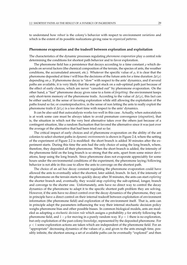
2.2 SHORTEST PATHS AS THE RESULT OF A SYNERGY OF INGREDIENTS 29
to understand how robust is the colony’s behavior with respect to environment variations and
which is the extent of its possible realizations giving raise to organized patterns.
Pheromone evaporation and the tradeoff between exploration and exploitation
The characteristics of the dynamic processes regulating pheromone evaporation play a central role
determining the conditions for shortest path behavior and to favor exploration.
The pheromone field has a persistence that decays according to a time constant ρ which de-
pends on several factors (the chemical composition of the terrain, the species of ants, the weather
conditions, the accumulated amount, etc.). Whatever the specific value of ρ, it is clear that the
pheromone deposited at time twill bias the decisions of the future ants for a time duration ∆t(ρ)
depending on ρ. If pheromone decay is “slow” with respect to the ants’ dynamics, and if several
paths are available, it is very likely that the ants get stuck on a sub-optimal path just because of
the effect of early choices, which are never “canceled out” by pheromone evaporation. On the
other hand, a “fast” pheromone decay gives raise to a form of forgetting: the environment keeps
only short-term memory of the pheromone trails. According to the value of ∆t(ρ), this fact can
be either useful, in the sense of favoring exploration while still allowing the exploitation of the
paths found so far, or counterproductive, in the sense of non letting the ants to really exploit the
pheromone trails if ∆t(ρ) is a too short time with respect to the ants’ dynamics.
It can be also said that autocatalysis works too well in this case. Actually, when autocatalysis
is at work some care must be always taken to avoid premature convergence (stagnation), that
is, the situation in which not the very best alternative takes over the others just because of a
contingent situation, like a random fluctuation that favored the alternative since it was just over
the average of the alternative that had been tried out so far.
The critical impact of early choices and of pheromone evaporation on the ability of the ant
colonies to select shortest paths in dynamic environments is shown in Figure 2.4, where the setting
of the experiment of Figure 2.2 is modified: the short branch is added 30 minutes after the ex-
periment starts. During this time the ants had the only choice of using the long branch, where,
therefore, they deposited all their pheromone. When the short branch is added, the intensity of
the pheromone field on the long branch is so strong that the ants, apart from some minor devi-
ations, keep using the long branch. Since pheromone does not evaporate appreciably for some
hours under the environmental conditions of the experiment, the pheromone laying/following
behavior is not able in this case to allow the ants to converge on the shortest path.
The choice of an ad hoc decay constant regulating the pheromone evaporation could have
allowed the ants to eventually select the shortest, later added, branch. In fact, if the intensity of
the pheromone on the terrain starts to quickly decay after 30 minutes, the ants can start exploring
the shorter branch and, eventually, they would stop exploiting the sub-optimal, longer, branch
and converge to the shorter one. Unfortunately, ants have no direct way to control the decay
dynamics of the pheromone to adapt it to the specific shortest path problem they are solving.
However, if the ants have no direct control over the decay dynamics of the pheromone, they can
in principle have a direct control on their internal tradeoff between exploitation of environment
information (the pheromone field) and exploration of the environment itself. That is, ants can
in principle adapt the parameters influencing the way their internal stochastic decision policy
weighs pheromone bias and other possible biases. In common biological models, ants are mod-
eled as adopting a stochastic decision rule which assigns a probability p for strictly following the
pheromone field, and 1− p for moving in a purely random way. If p = 1 there is no exploration,
but only exploitation of the past colony knowledge, represented by the deposited pheromone. For
p < 1 some exploration actions are taken which are independent of the pheromone field. For an
“appropriate” decreasing dynamics of the values of p, and given to the ants enough time, pos-
sibly infinite, the shortest among a set of available paths can be eventually “explored” and then

30 2. ANT COLONIES, THE BIOLOGICAL ROOTS OF ANT COLONY OPTIMIZATION
0
50
100
0-20 20-40 40-60 60-80 80-100
% o
ver n e
xper
imen
ts
% of ants selecting the shorter branch
n = 18, r = 2
Figure 2.4: Experiment with a binary bridge whose branches have different length. The basic setting is the same as inFigure 2.2. However, in this case the short branch is added 30 minutes after the experiment starts. During this timeants had the only choice of moving, and laying pheromone, on the long branch. The graph reports the distributionof the percentage of ants that selected the shorter branch over n = 18 experiments for the case of a bridge with thelong branch r = 2 times longer than the short one. The distribution refers to what happens after a transitory phase ofabout 10 minutes following the addition of the short branch. Modified from [203].
it can gradually attract the majority of the ants, if the general conditions of the experiment (e.g.,
pheromone evaporation dynamics and differential path lengths) can allow it. This asymptotic
behavior would closely remind that of a population-based (or direct-search) Simulated Anneal-
ing [375] with the decreasing of p playing the role of the decreasing temperature. Therefore, in a
sense, under appropriate “mild” mathematical conditions it can be conjectured that ant colonies
can always be able to asymptotically converge to the shortest path. Clearly, this is not true for
the finite/limited time case.
More in general, both pheromone evaporation and the characteristics of the ant stochastic
decision policy are strictly related to the issue of the tradeoff between exploitation (e.g., of a path
that seems to be particularly good) and exploration (e.g., of new alternative paths), which is a
major issue for any biological or artificial system engaged in search processes repeated over a
certain time interval (e.g., ACO).3 When multiple paths are in principle available or when the
characteristics of the environment dynamically change, it is immediately apparent the impor-
tance of being able to set an appropriate tradeoff between the exploitation of a current path that
appears to be good and the exploration of different alternatives. The issue becomes more and
more critical as the number of possible alternative “solutions” gets larger or the environment’s
changes become more and more frequent.
2.3 Robustness, adaptivity, and self-organization properties
Even if it is not always true that the shortest path behavior will arise, it is often the case that alter-
native non-random, self-organized, global patterns of activity will arise. That is, under reasonable
conditions (e.g., environmental conditions are not such that pheromone evaporates faster than
the average time necessary for an ant to reach the target), some interesting regular patterns can
be eventually observed. This fact witnesses the overall robustness of the mechanisms at work
3 The literature concerning the general mathematical aspects of the exploration/exploitation dilemma is vast, as well asthat on the strictly related bias/variance dilemma. References [248, 423] provide an insightful treatment of the subject inthe field of reinforcement learning (see Appendix E), in which the role of exploration is of central importance. The issueof bias/variance is treated in-depth in [196]. Most of the literature on the popular Simulated Annealing algorithm [253]is precisely about the definition of an appropriate balance between exploration and exploitation in general and practicalterms (e.g., see [367]).
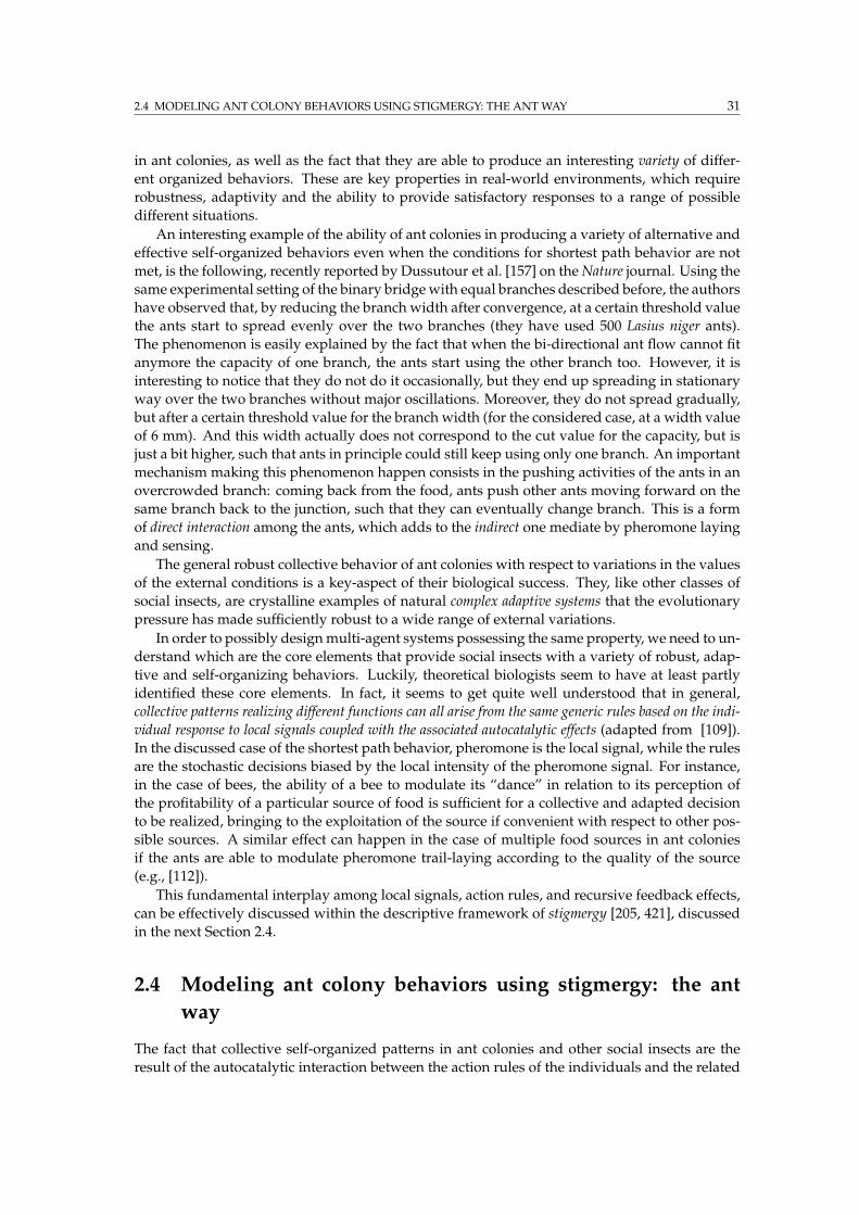
2.4 MODELING ANT COLONY BEHAVIORS USING STIGMERGY: THE ANTWAY 31
in ant colonies, as well as the fact that they are able to produce an interesting variety of differ-
ent organized behaviors. These are key properties in real-world environments, which require
robustness, adaptivity and the ability to provide satisfactory responses to a range of possible
different situations.
An interesting example of the ability of ant colonies in producing a variety of alternative and
effective self-organized behaviors even when the conditions for shortest path behavior are not
met, is the following, recently reported by Dussutour et al. [157] on theNature journal. Using the
same experimental setting of the binary bridgewith equal branches described before, the authors
have observed that, by reducing the branch width after convergence, at a certain threshold value
the ants start to spread evenly over the two branches (they have used 500 Lasius niger ants).
The phenomenon is easily explained by the fact that when the bi-directional ant flow cannot fit
anymore the capacity of one branch, the ants start using the other branch too. However, it is
interesting to notice that they do not do it occasionally, but they end up spreading in stationary
way over the two branches without major oscillations. Moreover, they do not spread gradually,
but after a certain threshold value for the branch width (for the considered case, at a width value
of 6 mm). And this width actually does not correspond to the cut value for the capacity, but is
just a bit higher, such that ants in principle could still keep using only one branch. An important
mechanism making this phenomenon happen consists in the pushing activities of the ants in an
overcrowded branch: coming back from the food, ants push other ants moving forward on the
same branch back to the junction, such that they can eventually change branch. This is a form
of direct interaction among the ants, which adds to the indirect one mediate by pheromone laying
and sensing.
The general robust collective behavior of ant colonies with respect to variations in the values
of the external conditions is a key-aspect of their biological success. They, like other classes of
social insects, are crystalline examples of natural complex adaptive systems that the evolutionary
pressure has made sufficiently robust to a wide range of external variations.
In order to possibly designmulti-agent systems possessing the same property, we need to un-
derstand which are the core elements that provide social insects with a variety of robust, adap-
tive and self-organizing behaviors. Luckily, theoretical biologists seem to have at least partly
identified these core elements. In fact, it seems to get quite well understood that in general,
collective patterns realizing different functions can all arise from the same generic rules based on the indi-
vidual response to local signals coupled with the associated autocatalytic effects (adapted from [109]).
In the discussed case of the shortest path behavior, pheromone is the local signal, while the rules
are the stochastic decisions biased by the local intensity of the pheromone signal. For instance,
in the case of bees, the ability of a bee to modulate its “dance” in relation to its perception of
the profitability of a particular source of food is sufficient for a collective and adapted decision
to be realized, bringing to the exploitation of the source if convenient with respect to other pos-
sible sources. A similar effect can happen in the case of multiple food sources in ant colonies
if the ants are able to modulate pheromone trail-laying according to the quality of the source
(e.g., [112]).
This fundamental interplay among local signals, action rules, and recursive feedback effects,
can be effectively discussed within the descriptive framework of stigmergy [205, 421], discussed
in the next Section 2.4.
2.4 Modeling ant colony behaviors using stigmergy: the ant
way
The fact that collective self-organized patterns in ant colonies and other social insects are the
result of the autocatalytic interaction between the action rules of the individuals and the related
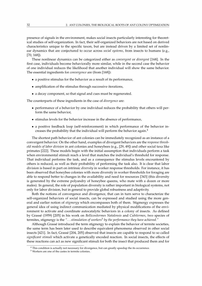
32 2. ANT COLONIES, THE BIOLOGICAL ROOTS OF ANT COLONY OPTIMIZATION
presence of signals in the environment, makes social insects particularly interesting for theoret-
ical studies of self-organization. In fact, their self-organized behaviors are not based on derived
characteristics unique to the specific taxon, but are instead driven by a limited set of nonlin-
ear dynamics that are conjectured to occur across social systems, from insects to humans (e.g.,
[70, 168]).
These nonlinear dynamics can be categorized either as convergent or divergent [168]. In the
first case, individuals become behaviorally more similar, while in the second case the behavior
of one individual reduces the likelihood that another individual will show the same behavior.
The essential ingredients for convergence are (from [168]):
• a positive stimulus for the behavior as a result of its performance,
• amplification of the stimulus through successive iterations,
• a decay component, so that signal and cues must be regenerated.
The counterparts of these ingredients in the case of divergence are:
• performance of a behavior by one individual reduces the probability that others will per-
form the same behavior,
• stimulus levels for the behavior increase in the absence of performance,
• a positive feedback loop (self-reinforcement) in which performance of the behavior in-
creases the probability that the individual will perform the behavior again.4
The shortest path behavior of ant colonies can be immediately recognized as an instance of a
convergent behavior. On the other hand, examples of divergent behaviors are the response thresh-
old models of labor division in ant colonies and honeybees (e.g., [29, 49]) and other social taxa like
primates [222]. These models begin with the initial assumption that individuals perform a task
when environmental stimuli reach a level that matches the individual’s threshold for response.
That individual performs the task, and as a consequence the stimulus levels encountered by
others is reduced, as well as their probability of performing the task also. It is clear that labor
division is based in part on intrinsic diversity in worker response thresholds. For instance, it has
been observed that honeybee colonies with more diversity in worker thresholds for foraging are
able to respond better to changes in the availability and need for resources [343] (this diversity
is generated by the extreme polyandry of honeybee queens, who mate with a dozen or more
males). In general, the role of population diversity is rather important in biological systems, not
only for labor division, but in general to provide global robustness and adaptivity.
Both the notions of convergence and divergence, that can in turn serve to characterize the
self-organized behaviors of social insects, can be expressed and studied using the more gen-
eral and earlier notion of stigmergy which encompasses both of them. Stigmergy expresses the
general idea of using indirect communication mediated by physical modifications of the envi-
ronment to activate and coordinate autocatalytic behaviors in a colony of insects. As defined
by Grasse (1959) [205] in his work on Bellicositermes Natalensis and Cubitermes, two species of
termites, stigmergy is the “. . . stimulation of workers5 by the performance they have achieved.”
Although Grasse introduced the term stigmergy to explain the behavior of termite societies,
the same term has been later used to describe equivalent phenomena observed in other social
insects [421]. In fact, Grasse [204, 205] observed that insects are capable to respond to so called
significant stimuli which activate a genetically encoded reaction. In social insects, the effects of
these reactions can act as new significant stimuli for both the insect that produced them and for
4 This condition is actually not necessary for divergence, but can greatly speedup the its occurrence.5 Workers are one of the castes in termite colonies.

2.4 MODELING ANT COLONY BEHAVIORS USING STIGMERGY: THE ANTWAY 33
other insects in the colony. The production of a new significant stimulus as a consequence of the
reaction to a significant stimulus, when iterated can be seen as an autocatalytic process that can
lead to a phase of a global coordination of the activities of the insects. Coordination in the sense
that each insect keeps acting autonomously and independently, but the effects of his/her actions
are synergistically combined with those of the other insects. The control of this coordination is
distributed and indirect: it is driven by the stimuli present in the environment, which, in turn,
are generated by the acting insects themselves. The whole process can be clearly seen as a form
of self-organization and is just a more general way of rephrasing what has already been said
making a distinction between the two specific cases of convergent and divergent behaviors.
However, speaking in terms of stigmergy is particularly interesting from an information pro-
cessing perspective since it allows to stress the indirect communication happening through the
individuals, and the role of so-called stigmergic variables [148], whose values can prime coordi-
nated behaviors. In order to use these notions also when we will refer to ACO’s artificial ants,
we give here a definition of stigmergy (and stigmergic variables) which slightly departs from
the Grasse’s original one:
DEFINITION 2.1 (Stigmergy and stigmergic variables): We call stigmergy any form of indirect com-
munication among a set of possibly concurrent and distributed agents which happens through acts of
local modification of the environment and local sensing of the outcomes of these modifications [147]. The
local environment’s variables whose value determine in turn the characteristics of the agents’ response,
are called stigmergic variables. Stigmergic communication and the presence of stigmergic variables is
expected (depending on parameter setting) to give raise to a synergy of effects resulting in self-organized
global behaviors.
Stigmergy as characterized here looks as a very specific form of communication aimed at
obtaining synergistic coordination and self-organization in a set of concurrent, and possibly dis-
tributed agents whose actions are driven by the value of stigmergic variables, local to the envi-
ronment. In the case of our ant colony, the stigmergic variables are clearly the pheromone trails.
On the other hand, in the case of a typical diverging situation, the stigmergic variable represent
the intensity of the local task that is waiting to be accomplished. For examples, the height of a
pile of dirty dishes in the sink can be seen in terms of stigmergic variable. Only when the value
of the variable, that is, the height of the pile, reaches some critical value one of the inhabitants of
the house will not be able to stand it anymore and will wash all or part of them, lowering in this
way the probability that somebody else will be engaged in the same task in the near future.
The characteristics of stigmergy, as well as the fact that this model is actually implemented
with success by all studied societies, suggest that it can be very effective to design multi-agent
systems thinking in stigmergic terms, in order to obtain an overall satisfactory level of synergy
from the agents’ actions resulting in robustness, scalability, adaptivity and a multiplicity of self-
organized behavioral patterns.
When a stigmergic approach is adopted, the focus is shifted from the design of the internal
characteristics of the single agents, which can be hopefully kept at a low level of complexity
and cost with respect to the required global task, to the design of: (i) an appropriate system
of indirect communication among the agents, and (ii) effective stigmergic variables such that
robust coordination and synergy can result from their combination. That is, the focus is put on
the definition of the protocols (interfaces), rather than of the modules (agents) of the system [100].
Protocols here are rules that prescribe allowed interfaces between modules, permitting system
functions that could not be achieved by isolated modules. Protocols also facilitate the addition
of new protocols, simplify modeling and abstraction. A good protocol (i.e., a good stigmergic
model) is one that supplies global robustness, scalability, evolvability, and, which, in the end,
allows to fully exploit the potentialities of the modules and of modularity.
34 2. ANT COLONIES, THE BIOLOGICAL ROOTS OF ANT COLONY OPTIMIZATION
It is clear that the design complexity is in a sense a “conserved” variable. In other words, the
intrinsic complexity associated to the global task to be accomplished is not changed by changing
the core design component which has to be engineered and optimized. There is a “price” to pay
in some form to eventually get the task realized by our system, and this price must be paid at
some level. It can be payed in terms of “agentware” by trying to design agents which are rather
complex and likely expensive in some either computational or economical sense. Otherwise,
by opting for a stigmergic approach, the price will be paid in terms of the design of the com-
munication mechanisms and stigmergic variables, and, possibly, by the use of a high number
of “cheap” agents, whatever cheap could mean in the considered context. This is the approach
likely followed by Nature for instance in the cases of ant colonies discovering shortest paths to
exploit food sources or termites building their nests [205]. The adaptation of coordinate behav-
iors over millions of years of evolution has been the price paid to face the intrinsic complexity of
these tasks with respect to the characteristics of the single insect.
In the following we will indicate with the term ant way (to problem-solving) the adoption
of a general stigmergic design model inspired by that implicitly adopted by the evolutionary
forces of Nature in the case of ant colonies. That is, a stigmergic model making use of a sig-
nificant number of computationally cheap concurrent and distributed agents, and relying on
either pheromone-like or threshold-like variables as stigmergic variables. In particular we will
be interested in the case in which the repertoire of the agents is such that each agent can in
principle output a complete solution for the problem at hand, but really good solutions are only
expected as the result of the stigmergic communication affecting the stigmergic variables of in-
terest. That is, the synergy among the agents is intended to obtain superior quality, not new
behaviors. Again, this is precisely what happens in the shortest path case: each ant can build a
path between nest and food but the discovery and convergence on the shortest path is expected
only as the result of the colony’s stigmergic interactions. And this is also what precisely happens
in ACO.
2.5 Summary
In this chapter the biological background of ACO has been fully acknowledged. We have de-
scribed and discussed the biological experiments that between the end of the 1980’s and the
beginning of the 1990’s have shown the ability of ant colonies to converge on the shortest be-
tween two possible paths connecting the colony’s nest to food sources. The general elements at
work (presence of a population of foraging ants, forward-backward path following, pheromone
laying and sensing, pheromone-biased stochastic decisions, autocatalysis, implicit path evalua-
tion, and iteration of the actions over time) have been identified and briefly discussed. We have
also showed the potential problems and limits intimately related to the approach. In particu-
lar, we have pointed out the role of pheromone and of the stochastic decision policy in terms
of exploration/exploitation tradeoff, and the fact that it becomes less likely that the colony can
converge to the shortest path if the number of alternative paths grows and/or the environment
is not really stationary. On the other hand, we have discussed the robustness of the ant behav-
iors. Ant colonies can in fact show a multiplicity of organized behaviors in response to different
external conditions. We have remarked that the observed self-organized behaviors are the result
of a few general nonlinear dynamics likely to be common to all societies. In the perspective of
using the mechanisms at work in ant colonies, and in social insects in general, as a reference to
guide the design of robust, adaptive, scalable, and flexible multi-agent systems, we have tried to
get a precise understanding of these dynamics. At this aim we have discussed them within the
more general stigmergy framework, which we have conveniently (re)defined. We have claimed
that stigmergic modeling is particularly suitable for multi-agent system design, also due to the

2.5 SUMMARY 35
fact that it focuses more on the level of the interactions (protocols) than on that of designing
really complex agents (modules), resulting in system that are expected to be robust, scalable,
adaptive and flexible (other than fully distributed). The “ant way”, a particular instance of stig-
mergic modeling directly derived from ant colony characteristics, is informally introduced, and
will serve, together with the fundamental notions of stigmergy and stigmergic variables (e.g.,
pheromone), to maintain a solid terminological and conceptual bridge between ACO and ant
colonies across the thesis.

36 2. ANT COLONIES, THE BIOLOGICAL ROOTS OF ANT COLONY OPTIMIZATION
CHAPTER 3
Combinatorial optimization,
construction methods, and
decision processes
This chapter provides the formal tools and the basic scientific background that will be used to
formally define and discuss ACO. Here we define/introduce those mathematical notions and
terms that are useful if not necessary to reason about ACO. With these notions in the hands we
will get a clear understanding of which are the really innovative ACO’s ideas, which are the
relationships between ACO and other frameworks for optimization and control, which are the
potentialities and the intrinsic limitations of ACO, and in which sense ACO’s basic design can
be modified and possibly improved.
Since we will discuss important general frameworks that can be seen as directly related to
ACO (and from which we can import results, ideas, models, etc.), the content of the chapter can
be seen as a sort of high-level “related work”, although discussions on related approaches are
practically spread all over the chapters.
The topics considered in this chapter are derived from the specific way ACO is seen in this
thesis, that is, in the terms of a multi-agent metaheuristic featuring solution construction, use of
memory, repeated solution sampling, and learning of the parameters of the construction policy
over a small subspace. According to this view, the chapter defines and/or discusses the char-
acteristics of: (i) the combinatorial optimization problems addressed by ACO, (ii) the model chosen
to represent the problem at hand, (iii) construction heuristics for combinatorial problems, (iv) the
equivalence between solution construction and sequential decision process, stressing the notion of
process state and the relationships with the fields of control [47], dynamic programming [20, 23],
and Markov decision processes [353], (v) the graphical tools (state graph, construction graph, and
influence diagrams) that can be used to represent and reason on the structure and dynamics
of construction processes, (vi) the notion of phantasma, defined as a subset of features of the
complete information state of the decision process, and, (vii) some of the different general ap-
proaches to optimization, in particular those using or not states and state-value functions (value-
based vs. policy-search), pointing out the differences in terms of used information and expected
finite-time performance.
The chapter is necessarily long since it deals with several general topics. However, we have
tried to minimize the overall redundancy, such that all the introduced notions are used some-
where in the following of the thesis. The chapter is not intended to provide a comprehensive
and detailed treatment of all the subjects that are considered, which would be out of the scope
of this thesis, but rather to give a bird-eye view, emphasizing the logical connections and some
of the most characterizing aspects. Therefore, more than focusing on the specific and detailed
properties of each topic, the chapter focuses on their reciprocal relationships and on their general
characteristics. A number of statements are not supported by formal explanations but rather by
38 3. COMBINATORIAL OPTIMIZATION, CONSTRUCTIONMETHODS, AND DECISION PROCESSES
pointing out published references. Examples are extensively used, usually to discuss subjects
that are very specific.
The original outcome of the chapter consists in putting on a same logical line several different
notions, disclosing their connections, and extracting their general core properties in relation to
combinatorial optimization issues.
Most of the chapter’s content comes from a reasoned composition of ideas obtained from
critical literature review. However, part of the ideas, and the link between ACO and control /
dynamic programming comes from the work on ant programming, which was co-authored with
Mauro Birattari and Marco Dorigo [33, 34]. Ant programming was introduced as a framework
that presents most of the characterizing features of ACO but which is more amenable to theoret-
ical analysis, and which allowed to bridge the terminological gap between ACO and the fields
of control [23] and reinforcement learning [442, 414]. The work on ant programming has given
a major contribution to the way ACO is seen in this thesis.
Organization of the chapter
The chapter starts defining and discussing the characteristics of the class of combinatorial op-
timization problems that are the target of ACO algorithms (Section 3.1), pointing out the dif-
ference between static and dynamic, distributed and centralized problems. Different ways of
defining compact representation for a combinatorial problem are discussed. Since problem so-
lutions are expressed in terms of subsets of components, Subsection 3.1.1 defines the precise
meaning of solution component, while Subsection 3.1.2 discusses the issue of using different
problem representations by adopting component sets with different characteristics.
Section 3.2 and all its subsections are devoted to the definition and discussion of construction
methods, that construct a solution by adding one more component at each construction step.
The generalities and definitions about construction methods are discussed in the first part of
the section, while Subsection 3.2.1 considers the properties of different general strategies for
including a new component into a building solution. Subsection 3.2.2 discusses the appropriate
domains of application of construction strategies as well as the definition of the cost values
that can be used to optimize the construction steps. In addition to this, Appendix B discusses
modification methods, which can be seen as complementary to the construction ones, since they
consider whole solutions at once, without passing through the steps of incremental construction.
Construction processes can be conveniently seen in the terms of decision processes. Section 3.3
shows the equivalence between construction and sequential decision processes. Subsection 3.3.1
goes further, discussing the equivalence between sequential decision tasks and control tasks.
This fact allows the introduction of the important notion of state of the process, or, equivalently,
of state of the problem. Problem states have precise characteristics which are discussed in Sub-
section 3.3.2 exploiting their representation in terms of a graph called state graph. The state graph
carries a lot of useful information concerning both the feasibility of a solution under construc-
tion and its quality. However, for large combinatorial problems the dimension of the state graph
explodes exponentially, therefore, Subsection 3.3.3 introduces a more compact graphical repre-
sentation of both the state structure and the dynamics of a construction process. This graphical
representation is termed construction graph, and coincides with the structure used in ACO to
frame experience in terms of pheromone variables and to take optimized decisions.
To understand generic decision processes, in order to get in turn a better understanding of
construction processes, it is necessary to take into consideration the framework of Markov de-
cision processes (MDP), which is the most important framework in the context of sequential de-
cision processes. Subsection 3.3.4 briefly introduces MDPs, discussing also the use of influence
diagrams to represent the MDP dynamics and some implications of the notion of state, making a
3.1 COMBINATORIAL OPTIMIZATION PROBLEMS 39
clear distinction between the underlying states of a systems and those of an agent representation.
Additional general information on MDPs and partially observable MDPs can be found in Ap-
pendix C. Subsection 3.3.5 discusses the situation in which the states of the problem are not fully
accessible to an optimization agent, that then has to rely on an incomplete representation of the
problem, with all the negative consequences of such a loss of important information. Actually,
this is the situation that ACO has to face, since for NP-hard problems the cardinality of the state
set is in general too large to use the states other than to check the feasibility of the solutions being
constructed. The notion of phantasma is defined to express the amount of information from the
past, different from state information, which is retained in order to take optimized decisions. The
connection between a specific phantasma representation and the process representation based
on both the construction and the state graph is also showed.
In the last part of the chapter the focus turns on the discussion of the characteristics of general
optimization strategies. Section 3.4, and Subsection 3.4.1 provide a view-in-the-large of some of
the most important classes of optimization algorithms. The last three subsections focus on two
large classes, which differ in the amount of information they make use of. From one side, there
is dynamic programming, or, more in general, value-based methods, which are exact methods
exploiting theMarkov structure of the state set and relying on the combined use of value functions
and Bellman’s optimality principle (Subsection 3.4.2). These methods can be very effective in
practice, but when the state set is too large, or the states are not accessible at all, they are virtually
ruled out. One can then rely on some form of approximation of the value functions, as it is
briefly discussed in Subsection 3.4.3. Otherwise, the more general policy search approach can be
adopted, which does not need to make use of value functions, or, more precisely, does not make
use of the Bellman’s relationships. Subsection 3.4.4 discusses some of the general properties of
policy search methods, as well as some of the choices that have to be issued when designing
a policy search algorithm. In particular, ACO will turn out to be a specific implementation of
a policy search algorithm. This finds its rationale in the fact that for the case of combinatorial
problems addressed by ACO it is in general computationally infeasible to rely on states and
value functions. ACO belongs to the class of policy search algorithms that transform the original
optimization problem into a learning problem on a small parametric subspace of the policies’
space. This is the final issue discussed in the chapter.
3.1 Combinatorial optimization problems
ACO is a metaheuristic for the solution of problems of combinatorial optimization. This section
provides a precise characterization of this class of problems.
DEFINITION 3.1 (Instance of a combinatorial optimization problem): An instance of a combinato-
rial optimization problem is a pair (S, J), where S is a finite set of feasible solutions and J is a function
that associates a real cost to each feasible solution, J : S → IR. The problem consists in finding the
element s∗ ∈ S which minimizes the function J :
s∗ = arg mins∈S
J(s). (3.1)
Hereafter only sets S with finite cardinality will be considered, even if the above definition
could be extended to countable sets of infinite cardinality. Given the finiteness of the set S, the
minimum of J on S indeed exists. If such minimum is attained for more than one element of S,
it is a matter of indifference which one is considered.
DEFINITION 3.2 (Combinatorial optimization problem): A combinatorial optimization problem is a
set of instances of an optimization problem.
40 3. COMBINATORIAL OPTIMIZATION, CONSTRUCTIONMETHODS, AND DECISION PROCESSES
The set of instances defining an optimization problem are usually all sharing some core prop-
erties or are all generated in a similar way. Therefore, an optimization problem defines a classi-
fication over sets of instances. This classification can be made according to several criteria that
are usually based on both mathematical and practical considerations.
In the following, the term solution is normally used to indicate a feasible solution in the set
S. More in general, the expression “solving the problem 3.1” will be normally used with the
meaning of proposing a solution s ∈ S. The solution itself can be or not an optimal one according
to the specific characteristics of the algorithm.
REMARK 3.1 (The specific class of problems addressed by ACO): ACO’s main target are difficult
instances of optimization combinatorial problems (typically belonging to NP-hard classes) for both the
cases of statically defined and dynamically changing characteristics of the instance.1
DEFINITION 3.3 (Static and dynamic optimization problems): Static combinatorial optimization
problems are such that the value of the mapping J does not change during the execution of the solv-
ing algorithm. In dynamically changing problems the mapping J changes during the execution of the
algorithm, that is, J depends on a time parameter t: J ≡ J(s, t).
If the statistical processes according to which the costs change over time are known in ad-
vance, then the optimization problem can be stated again as a static problem in which J is either
a function of the time or has a value drawn according to some probability distribution. In these
cases the minimization in Equation 3.1 has to be done according to the J ’s characteristics (e.g.,
minimization of the J ’s mean value, if J ’s values are drawn from a unimodal parametric distri-
bution). On the other hand, when only incomplete/insufficient information is available about
the dynamics of cost changes, the problem has to be tackled online using an adaptive approach.
The set of problems here labeled as “static” are actually most of the problems usually consid-
ered in combinatorial optimization textbooks (e.g., the traveling salesman problem, the quadratic
assignment problem, the graph coloring problem, etc.). They can be solved offline, adopting ei-
ther a centralized or a parallel/distributed approach according to the available computing resources.
Dynamic problems are somehow real-world versions of these problems. Routing in communica-
tion networks is a notable example of dynamic problem: the characteristics of both the input
traffic and the topology of the network can change over time according to dynamics for which
is usually hard to make robust prediction models. Moreover, in general routing requires a dis-
tributed problem solving approach (see Chapter 6).
Speaking in very general terms, while for static problems using a centralized or a distributed
algorithm is a matter of choice, dynamic problems usually impose more severe requirements,
such that the nature (either centralized or distributed) of the problem has to be matched by the
characteristics of the algorithm. In this sense, ACO’s design, relying on the use of a set of au-
tonomous agents, appears as rather effective, since it can be in principle used in both centralized
and distributed contexts with little adaptation.
Compact problem definitions
Usually, a combinatorial optimization problem, instead of being defined by directly providing
the solution set S, is defined in a compact way by means of mathematical relations. In the
domain of operations research a quite common way of defining an optimization problem is by
assigning a set of elements of interest, a set resulting from the possible ways to combine these
elements, and a set of restrictions that single out from this set the possible combinations that
identify the set S of the feasible solutions.
1 Appendix A contains brief descriptions for most of the combinatorial problems mentioned in this thesis. A compre-hensive classification of combinatorial problems and an extensive treatment of NP-hardness can be found in [344, 192].
3.1 COMBINATORIAL OPTIMIZATION PROBLEMS 41
These notions are made more precise in the definitions that follows (e.g., see [384, Chapter 1]):
DEFINITION 3.4 (Primitive, environment, and constraints sets): An optimization problem can be
formally identified in terms of a primitive set K, an environment set E, a solution set S, and a cost
criterion J defined on S. The primitive set defines the basic elements of the problem. The environment
set E is derived from the primitive set K as a subset of its power set, E ⊆ ℘(K), and the solution set
S is in turn derived from the environment set in terms of a family of subsets of E defined by a set of
mathematical relations Ω among the K’s elements, S ⊆ ℘(E) ∩ Ω. The set of relations Ω, which puts
specific limitations on the way the elements in E can be selected in order to identify elements in S, is
usually termed the constraints set.
The choices for setsK,E and Ω are not unique. Given an abstract definition of a problem, the
same problem can be expressed in different ways according to different choices for these sets.
One choice can be preferred over another just because it puts some more emphasis on aspects
that are seen asmore important in the considered context. In general, these facts raise the issue of
the representation adopted to model the abstract problem under consideration in the perspective
of attacking it with a specific class of algorithms. This issue is discussed more in depth in the
following of this section. But before that, it is useful to make the above notions of primitive and
environment sets more concrete through a few examples, and to introduce the notion of solution
components which will play a central role throughout the thesis.
In order to explain in what a problem definition in terms of the setsK,E and Ω precisely con-
sists of, let us consider the concrete case of two wide and quite general classes of combinatorial
problems: matching problems (e.g., [344, Chapters 10–11]) and set problems (e.g., [384, Chapter 1]),
to which we will refer often throughout the thesis:
Matching problems: A matching in a graph is a set of edges, no two of which share a node.
Goals in matching problems consist in finding either matchings with maximal edge sets
or, given that costs are associated to the edges/nodes, matchings with minimal associated
cost (weighted matching problems).
DEFINITION 3.5 (Matching problems in terms of primitive and environment sets): LetK =
1, 2, . . . , N be a generic set of elements of interest, and let K be the primitive set. The environ-
ment and solution sets are derived as follows:
E = ℘(K)
S = E ∈ E | problem constraints Ω(K) are satisfied(3.2)
The expressions 3.2 mean that the solution set is directly defined in terms of subsets ofK’s
power set. In the class of matching problems, of particular practical interest, as well as eas-
ier to solve, are those problems for which the underlying graph is a complete bipartite graph
with two sets of nodes that are equal in size.2 Bipartite weighted matchings of this type are
also known as assignment problems, which are for instance the problems of assigning tasks
to agents knowing the cost of making agent i deal with task j, and include important com-
binatorial problems like the TSP, the QAP and the VRP. Network flow problems can be also
expressed in terms of generic bipartite matching. The following example shows in practice
howK,E and S can be defined in the case of a TSP.
EXAMPLE 3.1: PRIMITIVE AND ENVIRONMENT SETS FOR THE TSP
Given anN -cities TSP,K = c1, c2, . . . , cN = 1, 2, . . . , N coincides with the set of the cities to2 A graph G(V, E) is said bipartite if the set of its vertices can be partitioned in two sets A and B such that each edge
in E has one vertex in A and one vertex in B.
42 3. COMBINATORIAL OPTIMIZATION, CONSTRUCTIONMETHODS, AND DECISION PROCESSES
be visited,E = ℘(K) is the set of all their possible combinations, and S results from the application
ofΩ as the subset of elements inE which are cyclic permutations of sizeN . An alternative definition
ofK,E and Ω could consist inK being the set of pairs (pi, cj), pi, cj ∈ 1, 2, . . . , N, that is, theset of elements telling that city cj is in position pi in the solution sequence (notice that being the
TSP’s solutions cyclic permutations, the notion of position requires setting an arbitrary start city).
In this case E is still the power set of K, but the syntax of the Ω relations is slightly different
from before, S is in fact defined as S =
Ek ∈ E, Ek = (pk1 , ck1), . . . , (pkN , ckN ) | ∪i pki =
1, . . . , N ∧ ∪i cki = 1, . . . , N
.That is, the set of pairs must correspond to a permutation
over 1, . . . , N.
Set problems: In assignment problems solutions can be usually expressed in terms of ordered
subsets of primitive elements, while in the case of set problems there is no explicit notion of
ordering. Moreover, in most of the assignment problems the solution has a predefined size,
while this is never the case for set problems. Set problems are also in general characterized
by an additional level of complexity with respect to the assignment ones in the sense that
is well expressed by the structure of the environment and solution sets:
DEFINITION 3.6 (Set problems in terms of primitive and environment sets): In set problems,
which can be further classified in set covering, set packing and set partitioning problems, the
corresponding of expression 3.2 takes the following form:
E = E ∈ ℘(K) | instance constraints ΩI are satisfiedS = E ′ ∈ ℘(E) | problem constraints Ω(K) are satisfied
(3.3)
These expressions point out the fact that the solution set is defined in a more complex
way than in the matching case. Solutions are in this case sets of subsets of elements of
the environment set, which, in turn, are subsets of elements of K. The ΩI constraints,
that have been called a bit improperly “instance constraints”, are defined by the actual
characteristics of the instance at hand.
The following example, which considers the specific case of a set covering problem, can
help to clarify the relationships amongK,E and S for this class of problems.
EXAMPLE 3.2: PRIMITIVE AND ENVIRONMENT SETS FOR THE SET COVERING PROBLEM
A general (unweighted) set covering problem (SCP) is defined as follows:
min |E ′|⋃
E′i∈E′
E ′i = K
E ′ ∈ ℘(E) ∩ Ω(K)
(3.4)
That is, the task is to find a family E ′ of subsets of elements of the power set ofK such that the car-
dinality of this family is minimal and all the elements in the primitive set K are “covered” by the
union of the elements in the family. This is for example the problem that airlines or train companies
have to deal with in order to optimize the assignment of personnel crews to cover transportation
routes. In these cases,K is the set of all routes that have to be covered. Groups of routes can be cov-
ered in principle by the same crew, such that the problem instance comes with possibly overlapping
subsets E of routes, which define the setE (which is the subset ofK’s power set identified by the spe-
cific instance’s data). The problem’s constraints Ω(K) tells that all the routes have to be covered by
3.1 COMBINATORIAL OPTIMIZATION PROBLEMS 43
at least one crew. Therefore, a feasible solution is a set E ′ of groups of routes, E ′ = E1, E2, . . . , En,with the meaning that a separate crew is allocated for each route group Ei. The goal is the mini-
mization of the number of crews (costs) used to cover all the required routes. The problem can be
made more complex by introducing different costs associated to cover each specific group of routes.
SCPs instances are commonly represented in terms of a 0, 1 matrix, whose rows coincides with
the routes of the example, and columns corresponds to crews covering different groups of routes. In
the problem instance 1 entries along column j indicate the set of routes (rows) covered by the j-th
crew (column).
Instead of relying on the use of primitive and environment sets which well characterize the
problem but their precise definition might be not really straightforward in some cases, in the
following we will mostly make use of the related notion of solution components to characterize
optimization problems:
DEFINITION 3.7 (Instance of a combinatorial problem using a compact representation): Let C be
a finite set of variables such that a solution in S can be expressed in terms of subsets of C’s elements. In
particular, called X ′ = ℘(C), S is identified by the subset of elements of X ′ for which the relations in Ω
are satisfied: S ⊆ X ′ ∩ Ω(C). Therefore, given the sets S,C and Ω(C), together with a real-valued cost
function J(S), a problem of combinatorial optimization consists in finding the element s∗ such that:
s∗ = arg mins∈X′ ∩ Ω(C)
J(s). (3.5)
Following this representation, an instance of a combinatorial optimization problem can be also compactly
represented by the triple
〈C,Ω, J〉. (3.6)
The elements of C, which represent the object of the decisions of the optimization process, are called
hereafter solution components.
3.1.1 Solution components
From definition 3.7 it is apparent that solution components always have a precise relationship
with the primitive and environment sets. In particular, for assignment problems C coincides
withK, while for set problemsC coincides withE. However, here we prefer to speak in terms of
solution components rather than primitive and environment sets, because of their more intuitive
and general meaning of parts of which a solution is composed of :
DEFINITION 3.8 (Solution components): The solution components set C is operatively defined as the
set from which a step-by-step decision process would select elements one-at-a-time and add them to a set
x until a feasible solution is built, that is, until x ∈ S.3
According to this characterization, the notion of solution components plays a central role in
this thesis, since combinatorial optimization is here framed in the domain of decision processes,
3 In general a solution to a combinatorial problem can be either expressed by means of ordered sets (sequences) orby means of unordered sets. However, the difference between ordered and unordered sets can be always removed byexpressing a generic sequence of components 〈c0, c1, . . . , cni 〉 as an unordered set whose elements are pairs of type(t, ci), t ∈ IN, with t representing the position index in the sequence. That is, by re-defining the original componentset C as: C′ : C × IN and reasoning on both the pair components. Therefore, in the following a solution will usuallybe referred to generically as a set, dropping off the distinction between ordered and unordered sets when not strictlynecessary.
44 3. COMBINATORIAL OPTIMIZATION, CONSTRUCTIONMETHODS, AND DECISION PROCESSES
and the components of a solution are precisely the step-by-step objects considered by the deci-
sions processes. More specifically, ACO’s target will consists in the learning of good decisions
in the terms of pairs of components to be included in the building solutions.
Definition 3.8 implicitly implies that for each set C of solution components must exist a bi-
jective mapping:
fC : X ⊆ ℘(C)→ S, (3.7)
such that each si ∈ S has a finite subset c1i , c2i , . . . , cni
i ∈ X of solution components as preimage
in X , and this preimage is unique. That is, after a finite number of decision steps, where at each
step t a new component ct is included in the set xt, the elements in xt ∈ X are expected to
map through fC onto an element s ∈ S. The characteristics of the mapping fC define the level
of correspondence between the problem under solution and the way solutions are represented.
In particular, if fC is not anymore surjective, not all the feasible solutions are going to have a
preimage in terms of a single set of components. Such a choice could rule out the same possibility
of addressing the optimal solution. On the other hand, if fC is not anymore injective, the same
solution in S can be addressed by one or more distinct elements in X . Such a choice would
result in a sort of blurred image of the solution set as seen from the component set, since several
solutions could be seen as the same solution, making potentially difficult for an algorithm to
act optimally. In general, when the mapping fC is not anymore bijective the representation will
undergo some loss of necessary information. That is, additional information/elements must be
added to a subset x ∈ X of C’s elements in order to map it onto a solution.
In the following, if not explicitly stated, it is always assumed that a lossless representation
model is being used. This is usually the case also for ACO implementations. The rationale
behind the possible use of lossy models is briefly discussed in the next subsection.
It is clear that once a mapping fC has been defined, solution components can be seen in more
general terms as decision variables. At each solution construction step a decision variable ct rep-
resenting any convenient value is assigned. The only strict requirement consists in the fact that
sets of decision variables can be eventually mapped bijectively onto a feasible solution. Since in
some sense it is natural to explicitly associate decision variables to parts of a solution, in the fol-
lowing we will preferably use the term “solution components” instead of “decision variables”.4
Even if this latter would likely make clearer the intrinsic meaning of ACO’s pheromone vari-
ables, which are precisely associated to pairs (ci, cj) of decision variables: decision cj is taken,
conditionally to the fact that decision ci has been already issued, according to a probability value
which depends on the value of the pheromone variable τcicjassociated to the pair of decisions
(and ACO’s activities are aimed at learning the τ ’s values in order to identify good decisions).
The way ACO is discussed in this thesis in terms of sequential decision processes, as well as the
recent work of Chang et al. [76], where ACO, departing from the usual application to “classi-
cal” combinatorial optimization problems, is applied to the solution of generic MDPs (therefore,
dealing with stochastic transitions after the issuing of a decision), strongly confirm this inter-
changeable view of pheromone variables as pairs of decision variables or solution components.
3.1.2 Characteristics of problem representations
An optimization problem (S, J) can be represented according to different models of the form
〈C,Ω, J〉 (or, equivalently, according to different choices of primitive and environment sets).
That is, the sets C and Ω (and, consequently, fC), can be in principle chosen in a number of
different ways, possibly according to different points of view, yet defining the same abstract
class of problems. However, different choices can result in rather different ways of looking at
and solving the same problem. One example can help to clarify the issue.
4 Also due to the fact that in the ACO’s definition [138] only the term solution component has been used. Such thatthis term in now widely in use in the ACO’s community.
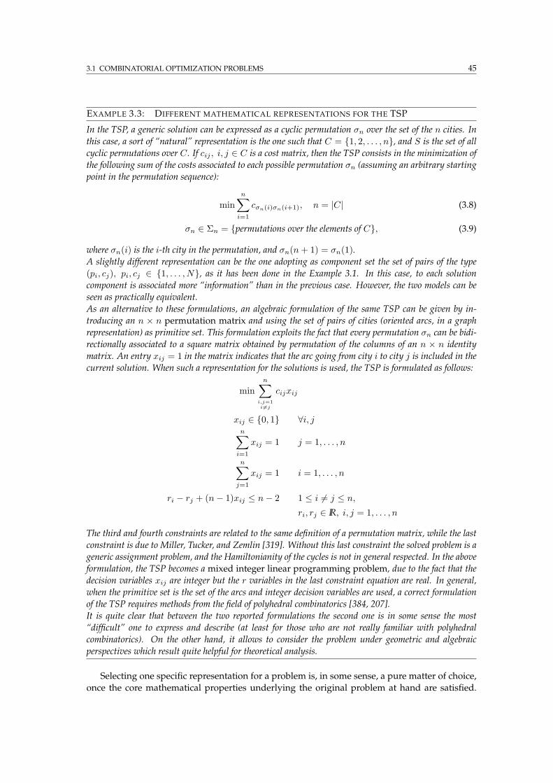
3.1 COMBINATORIAL OPTIMIZATION PROBLEMS 45
EXAMPLE 3.3: DIFFERENT MATHEMATICAL REPRESENTATIONS FOR THE TSP
In the TSP, a generic solution can be expressed as a cyclic permutation σn over the set of the n cities. In
this case, a sort of “natural” representation is the one such that C = 1, 2, . . . , n, and S is the set of all
cyclic permutations over C. If cij , i, j ∈ C is a cost matrix, then the TSP consists in the minimization of
the following sum of the costs associated to each possible permutation σn (assuming an arbitrary starting
point in the permutation sequence):
min
n∑
i=1
cσn(i)σn(i+1), n = |C| (3.8)
σn ∈ Σn = permutations over the elements of C, (3.9)
where σn(i) is the i-th city in the permutation, and σn(n+ 1) = σn(1).
A slightly different representation can be the one adopting as component set the set of pairs of the type
(pi, cj), pi, cj ∈ 1, . . . , N, as it has been done in the Example 3.1. In this case, to each solution
component is associated more “information” than in the previous case. However, the two models can be
seen as practically equivalent.
As an alternative to these formulations, an algebraic formulation of the same TSP can be given by in-
troducing an n × n permutation matrix and using the set of pairs of cities (oriented arcs, in a graph
representation) as primitive set. This formulation exploits the fact that every permutation σn can be bidi-
rectionally associated to a square matrix obtained by permutation of the columns of an n × n identity
matrix. An entry xij = 1 in the matrix indicates that the arc going from city i to city j is included in the
current solution. When such a representation for the solutions is used, the TSP is formulated as follows:
minn∑
i,j=1
i6=j
cijxij
xij ∈ 0, 1 ∀i, jn∑
i=1
xij = 1 j = 1, . . . , n
n∑
j=1
xij = 1 i = 1, . . . , n
ri − rj + (n− 1)xij ≤ n− 2 1 ≤ i 6= j ≤ n,ri, rj ∈ IR, i, j = 1, . . . , n
The third and fourth constraints are related to the same definition of a permutation matrix, while the last
constraint is due to Miller, Tucker, and Zemlin [319]. Without this last constraint the solved problem is a
generic assignment problem, and the Hamiltonianity of the cycles is not in general respected. In the above
formulation, the TSP becomes a mixed integer linear programming problem, due to the fact that the
decision variables xij are integer but the r variables in the last constraint equation are real. In general,
when the primitive set is the set of the arcs and integer decision variables are used, a correct formulation
of the TSP requires methods from the field of polyhedral combinatorics [384, 207].
It is quite clear that between the two reported formulations the second one is in some sense the most
“difficult” one to express and describe (at least for those who are not really familiar with polyhedral
combinatorics). On the other hand, it allows to consider the problem under geometric and algebraic
perspectives which result quite helpful for theoretical analysis.
Selecting one specific representation for a problem is, in some sense, a pure matter of choice,
once the core mathematical properties underlying the original problem at hand are satisfied.
46 3. COMBINATORIAL OPTIMIZATION, CONSTRUCTIONMETHODS, AND DECISION PROCESSES
However, the choice of a specific representation in a sense defines the model used by the algo-
rithm designer to figure the solutions, and, therefore, the way of thinking about the problem. As
also shown by several experiments conducted by cognitive scientists, different representations
for the solution of a same problem defined in a rather abstract way, can easily suggest different
strategies depending also on the person’s background, and, therefore, can lead to final solutions
of different quality.5
Representations can differ not only in the sense of the used language, but also concerning the
amount of information about the “original” problem that is retained in the working model. The
choice of adopting one representation model over another can be explicitly dictated by the inten-
tion of feeding to the class of algorithms at hand amodel which is: (i) particularly appropriate for
the algorithms’ characteristics, or (ii) in some sense easier to deal with, in the hope/conviction
that the possible loss of information will not critically affect the ability of the algorithm to find
optimal/good solutions.
These issues are pointed out here since, as it is explained in the following chapters, an impor-
tant preliminary step in the design of an ACO algorithm precisely consists in the definition of
the solution components model which is fed to the ant agents for solution construction and de-
cision learning. And the characteristics of this model greatly affect the final performance of the
algorithm. It will be shown that ACO implementations usually adopts lossless representations, but at
the same time an important loss of information happens for what concerns the variables that are
ACO’s learning target. However, to understand this point it will be necessary to introduce the
notion of state, which is based, in turn, on that of solution components.
3.2 Construction methods for combinatorial optimization
ACO’s ant-like agents independently generate solutions according to an incremental construc-
tion process. Therefore, the notion of construction algorithm is at the core of ACO. A generic
construction algorithm is defined here as follows:6
DEFINITION 3.9 (Construction algorithm): Given an instance of the generic combinatorial optimiza-
tion problem in the form 3.5, an algorithm is said a construction algorithm when, starting from an
empty partial solution x0 = ∅, a complete solution s ∈ S is incrementally built by adding one-at-a-time
a new component c ∈ C to the partial solution.
The generic iteration (also termed hereafter transition) of a construction process can be described as:
xj = c1, c2, . . . , cj → xj+1 = c1, c2, . . . , cj , cj+1, ci ∈ C, ∀i ∈ 1, 2, . . . , |C|, (3.10)
where xj ∈ X ′ = ℘(C) is a partial solution of cardinality (length) j, j ≤ |C| <∞.
The algorithmic skeleton of a generic construction strategy is reported in the pseudo-code of
the Algorithm box 3.1.
The pseudo-code describes in a compact way the general characteristics of a construction pro-
cess, which are:7
• the starting point is a possibly empty partial solution;
5 The work of Zhang [449] contains some useful references and makes an interesting study on group behaviors inrelationship to the adoption of different representations.
6 See Appendix B for a discussion on modification methods, which can be seen as a complementary general approachto optimization.
7 In the following the terms process, agent, algorithm and strategy are often freely used as synonyms when this wouldnot provoke misunderstandings. Therefore, expressions like “construction agent” or “construction process” will havethe same practical meaning. However, the explicit use of the term agent will be also used, for instance, with the purposeof stressing the characteristics of autonomy of the process of solution construction.
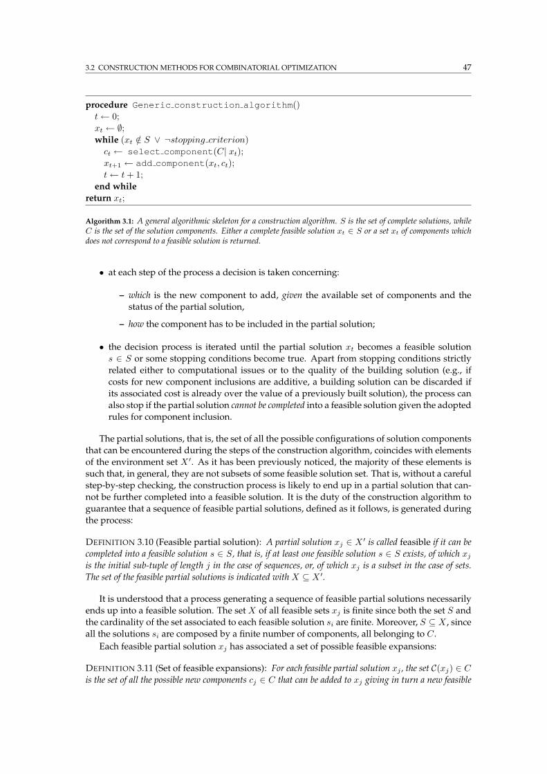
3.2 CONSTRUCTIONMETHODS FOR COMBINATORIAL OPTIMIZATION 47
procedure Generic construction algorithm()
t← 0;
xt ← ∅;while (xt /∈ S ∨ ¬stopping criterion)
ct ← select component(C| xt);xt+1 ← add component(xt, ct);
t← t+ 1;
end while
return xt;
Algorithm 3.1: A general algorithmic skeleton for a construction algorithm. S is the set of complete solutions, whileC is the set of the solution components. Either a complete feasible solution xt ∈ S or a set xt of components whichdoes not correspond to a feasible solution is returned.
• at each step of the process a decision is taken concerning:
– which is the new component to add, given the available set of components and the
status of the partial solution,
– how the component has to be included in the partial solution;
• the decision process is iterated until the partial solution xt becomes a feasible solution
s ∈ S or some stopping conditions become true. Apart from stopping conditions strictly
related either to computational issues or to the quality of the building solution (e.g., if
costs for new component inclusions are additive, a building solution can be discarded if
its associated cost is already over the value of a previously built solution), the process can
also stop if the partial solution cannot be completed into a feasible solution given the adopted
rules for component inclusion.
The partial solutions, that is, the set of all the possible configurations of solution components
that can be encountered during the steps of the construction algorithm, coincides with elements
of the environment set X ′. As it has been previously noticed, the majority of these elements is
such that, in general, they are not subsets of some feasible solution set. That is, without a careful
step-by-step checking, the construction process is likely to end up in a partial solution that can-
not be further completed into a feasible solution. It is the duty of the construction algorithm to
guarantee that a sequence of feasible partial solutions, defined as it follows, is generated during
the process:
DEFINITION 3.10 (Feasible partial solution): A partial solution xj ∈ X ′ is called feasible if it can be
completed into a feasible solution s ∈ S, that is, if at least one feasible solution s ∈ S exists, of which xjis the initial sub-tuple of length j in the case of sequences, or, of which xj is a subset in the case of sets.
The set of the feasible partial solutions is indicated with X ⊆ X ′.
It is understood that a process generating a sequence of feasible partial solutions necessarily
ends up into a feasible solution. The set X of all feasible sets xj is finite since both the set S and
the cardinality of the set associated to each feasible solution si are finite. Moreover, S ⊆ X , since
all the solutions si are composed by a finite number of components, all belonging to C.
Each feasible partial solution xj has associated a set of possible feasible expansions:
DEFINITION 3.11 (Set of feasible expansions): For each feasible partial solution xj , the set C(xj) ∈ Cis the set of all the possible new components cj ∈ C that can be added to xj giving in turn a new feasible
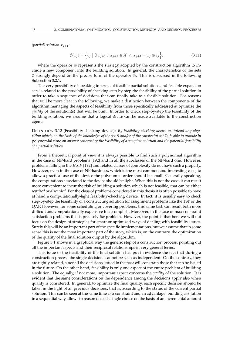
48 3. COMBINATORIAL OPTIMIZATION, CONSTRUCTIONMETHODS, AND DECISION PROCESSES
(partial) solution xj+1:
C(xj) =
cj∣
∣ ∃ xj+1 : xj+1 ∈ X ∧ xj+1 = xj ⊕ cj
, (3.11)
where the operator ⊕ represents the strategy adopted by the construction algorithm to in-
clude a new component into the building solution. In general, the characteristics of the sets
C strongly depend on the precise form of the operator ⊕. This is discussed in the following
Subsection 3.2.1.
The very possibility of speaking in terms of feasible partial solutions and feasible expansion
sets is related to the possibility of checking step-by-step the feasibility of the partial solution in
order to take a sequence of decisions that can finally take to a feasible solution. For reasons
that will be more clear in the following, we make a distinction between the components of the
algorithm managing the aspects of feasibility from those specifically addressed at optimize the
quality of the solution(s) that will be built. In order to check step-by-step the feasibility of the
building solution, we assume that a logical device can be made available to the construction
agent:
DEFINITION 3.12 (Feasibility-checking device): By feasibility-checking device we intend any algo-
rithm which, on the basis of the knowledge of the set S and/or of the constraint set Ω, is able to provide in
polynomial time an answer concerning the feasibility of a complete solution and the potential feasibility
of a partial solution.
From a theoretical point of view it is always possible to find such a polynomial algorithm
in the case of NP-hard problems [192] and in all the subclasses of the NP-hard one. However,
problems falling in theEXP [192] and related classes of complexity do not have such a property.
However, even in the case of NP-hardness, which is the most common and interesting case, to
allow a practical use of the device the polynomial order should be small. Generally speaking,
the computations associated to the device should be light. When this is not the case, it can result
more convenient to incur the risk of building a solution which is not feasible, that can be either
repaired or discarded. For the class of problems considered in this thesis it is often possible to have
at hand a computationally-light feasibility-checking device. In fact, it is usually easy to check
step-by-step the feasibility of a constructing solution for assignment problems like the TSP or the
QAP. However, for some scheduling or covering problems, this same task can result both more
difficult and computationally expensive to accomplish. Moreover, in the case of max constraint
satisfaction problems this is precisely the problem. However, the point is that here we will not
focus on the design of strategies for smart or optimized ways of dealing with feasibility issues.
Surely this will be an important part of the specific implementations, but we assume that in some
sense this is not the most important part of the story, which is, on the contrary, the optimization
of the quality of the final solution output by the algorithm.
Figure 3.1 shows in a graphical way the generic step of a construction process, pointing out
all the important aspects and their reciprocal relationships in very general terms.
This issue of the feasibility of the final solution has put in evidence the fact that during a
construction process the single decisions cannot be seen as independent. On the contrary, they
are tightly related, since all the decisions issued in the past will constrain those that can be issued
in the future. On the other hand, feasibility is only one aspect of the entire problem of building
a solution. The equally, if not more, important aspect concerns the quality of the solution. It is
evident that the same considerations on the dependence among the decisions apply also when
quality is considered. In general, to optimize the final quality, each specific decision should be
taken in the light of all previous decisions, that is, according to the status of the current partial
solution. This can be seen at the same time as a constraint and an advantage: building a solution
in a sequential way allows to reason on each single choice on the basis of an incremental amount
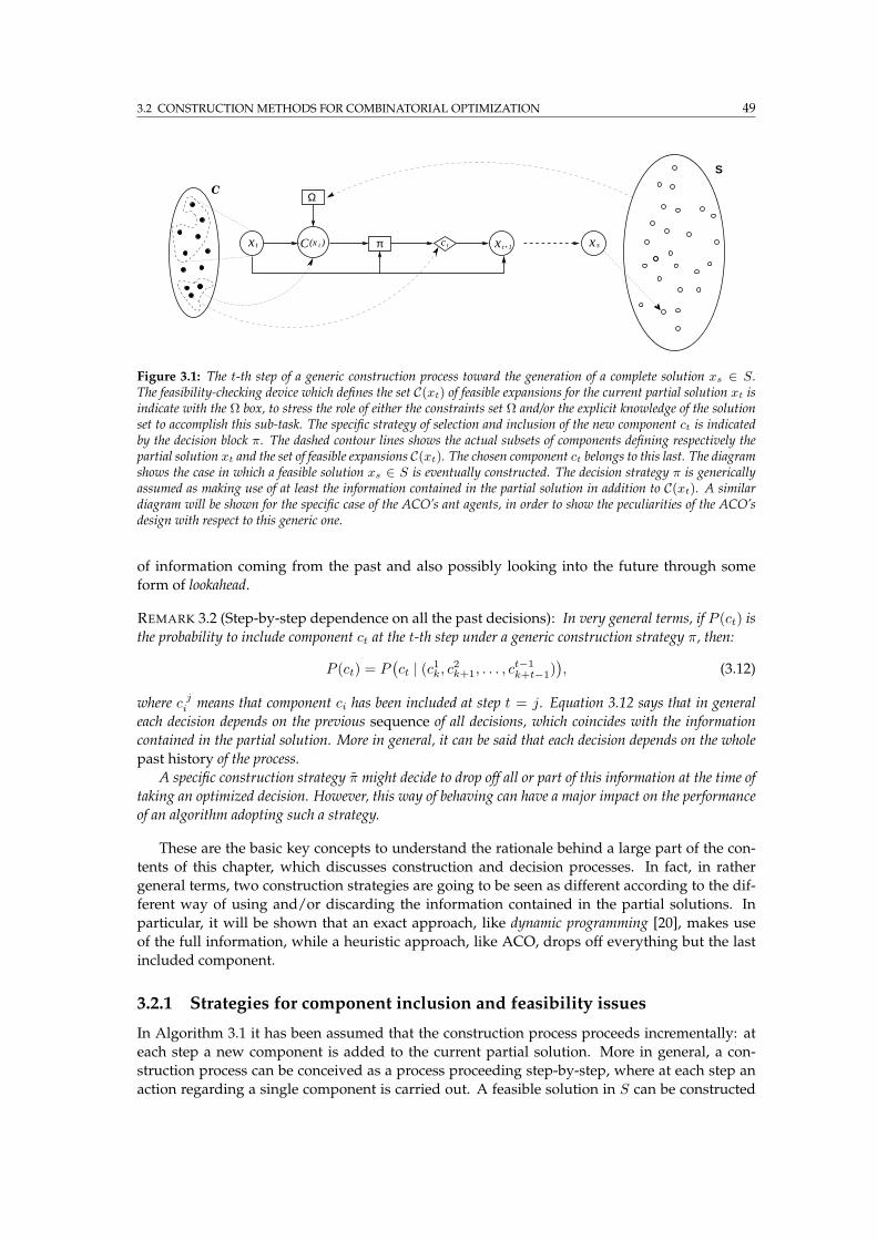
3.2 CONSTRUCTIONMETHODS FOR COMBINATORIAL OPTIMIZATION 49
S
Ω
tcx t x s t(x )
C
π x t+1C
Figure 3.1: The t-th step of a generic construction process toward the generation of a complete solution xs ∈ S.The feasibility-checking device which defines the set C(xt) of feasible expansions for the current partial solution xt isindicate with the Ω box, to stress the role of either the constraints set Ω and/or the explicit knowledge of the solutionset to accomplish this sub-task. The specific strategy of selection and inclusion of the new component ct is indicatedby the decision block π. The dashed contour lines shows the actual subsets of components defining respectively thepartial solution xt and the set of feasible expansions C(xt). The chosen component ct belongs to this last. The diagramshows the case in which a feasible solution xs ∈ S is eventually constructed. The decision strategy π is genericallyassumed as making use of at least the information contained in the partial solution in addition to C(xt). A similardiagram will be shown for the specific case of the ACO’s ant agents, in order to show the peculiarities of the ACO’sdesign with respect to this generic one.
of information coming from the past and also possibly looking into the future through some
form of lookahead.
REMARK 3.2 (Step-by-step dependence on all the past decisions): In very general terms, if P (ct) is
the probability to include component ct at the t-th step under a generic construction strategy π, then:
P (ct) = P(
ct | (c1k, c2k+1, . . . , ct−1k+t−1)
)
, (3.12)
where c ji means that component ci has been included at step t = j. Equation 3.12 says that in general
each decision depends on the previous sequence of all decisions, which coincides with the information
contained in the partial solution. More in general, it can be said that each decision depends on the whole
past history of the process.
A specific construction strategy π might decide to drop off all or part of this information at the time of
taking an optimized decision. However, this way of behaving can have a major impact on the performance
of an algorithm adopting such a strategy.
These are the basic key concepts to understand the rationale behind a large part of the con-
tents of this chapter, which discusses construction and decision processes. In fact, in rather
general terms, two construction strategies are going to be seen as different according to the dif-
ferent way of using and/or discarding the information contained in the partial solutions. In
particular, it will be shown that an exact approach, like dynamic programming [20], makes use
of the full information, while a heuristic approach, like ACO, drops off everything but the last
included component.
3.2.1 Strategies for component inclusion and feasibility issues
In Algorithm 3.1 it has been assumed that the construction process proceeds incrementally: at
each step a new component is added to the current partial solution. More in general, a con-
struction process can be conceived as a process proceeding step-by-step, where at each step an
action regarding a single component is carried out. A feasible solution in S can be constructed

50 3. COMBINATORIAL OPTIMIZATION, CONSTRUCTIONMETHODS, AND DECISION PROCESSES
by acting upon the set of solution components starting from the empty set, x0 = ∅, and by
iteratively executing one of the following three operations:
• Oi, inclusion of a new component,
• Or, replacement of a previously included component,
• Od, deletion of a previously included component.
Therefore, at the j-th step of the process, conditionally depending on the current partial solution,
a component cj ∈ C and an operation oj ∈ Oi, Or, Od are chosen, and the partial solution is
consequently modified. The construction process can end when the resulting xj+1 is a complete
solution or according to some other convenient stopping criteria.
In the previous case of using only the operation Oi, in order to obtain the final feasibility of
the building solution a feasibility-checking device was assumed as necessary. On the other hand,
if all the three operations can be freely used, the feasibility-checking device is still necessary but
it can be in some sense less precise for what concerns the feasibility of partial solutions. In fact,
in this case, at each step a partial solution can grow (Oi), or it can be modified without changing
its size (Or), or it can shrink (Od) by removing previous choices. As a consequence, since it is
always possible to fully repair or backtrack previous choices, it is in principle always possible to
end up in a feasible solution, if the characteristics of the construction process can allow it. On
the other hand, this great flexibility is payed in terms of possibility of cycles generation, lengthy
construction processes, complex decision strategies to implement (both the operation and the
component to act upon must be decided at each step).
These can be seen all as negative features in the perspective of designing and analyzing effi-
cient construction algorithms. Accordingly, as it is shown in the following, the design choice of
ACO has been that ofmainly restricting the use to the inclusion operation. With this choice cycles
are not anymore possible, partial solutions undergo strictly monotonic growth, and the number
of possible alternatives at each construction step is much reduced. Certainly, a lot of flexibility
is also lost but the basic operation Oi is still powerful enough to allow the construction of op-
timal solutions. In some sense, this choice represents a reasonable tradeoff between flexibility
and computational and design complexity. According to these facts, in the following, in both
the general and ACO-specific discussions, it is assumed that the used operation is always the
inclusion one.
With this choice in principle ACO would need an “accurate” feasibility-checking device in
order to guarantee the feasibility of the solutions. However, even when it is not computationally
convenient to run such an accurate device, the very possibility of discarding some of the con-
structing solutions because of feasibility problems can be seen as in accordance with the general
philosophy of the ACO’s approach, and, more in general, with the philosophy of the “ant way”,
based on the quick generation of a number of independent solutions. In this sense, a small per-
centage of solution that have to be discarded is not expected to really affect the outcome of the
whole optimization process.
REMARK 3.3 (Feasibility and quality in ACO): In ACO, the component concerning the feasibility
of the constructed solutions is kept logically separated from that concerning their quality. That is, the
ability to quickly construct feasible solutions (or a large majority of feasible solutions) is given for granted
in ACO’s design, the focus being on the ability to optimize their quality.
Extension and insertion strategies for component inclusion
For the case of solutions expressed in terms of ordered sets, twomajor strategies I for component
inclusion can be identified:
3.2 CONSTRUCTIONMETHODS FOR COMBINATORIAL OPTIMIZATION 51
• Ie: extension of the solution by addition at the end of the sequence,
• Ii: insertion at any position,
In the case of unordered sets, extension and insertion strategies are indistinguishable. Therefore,
considering the case of sequences, if cj+1 is the component selected for inclusion at the j + 1-
th step of the process and xj = (c1, c2, . . . , cj) is the current partial solution, then, the (partial)
solution at step j + 1 becomes:
• Extension case:
xj+1 = (c1, c2, . . . , cj , cj+1).
• Insertion case:
xj+1 = (c1, c2, . . . , ci−1, cj+1, ci, . . . , cj).
In this case, the insertion of the new component can happen at any position i ∈ 1, 2, . . . , j.In particular, i can correspond to the last position, such that the extension case can be ac-
tually seen as a particular case of the insertion one.
3.2.2 Appropriate domains of application for construction methods
The application of construction algorithms appears as appropriate when the cost J(s) of a so-
lution s can be expressed as a combination of contributions each one related to the fact that a
particular component cj is included into the partial solution solution xj . The cost can be either
associated to the inclusion of the component itself, or, more in general, to the component condi-
tionally depending on the current partial solution. This means that a real-valued transition cost
function J must be defined either on the set X of the partial solutions, or on the set C of the so-
lution components. The importance of such a cost function consists in the fact that it can be used
by the step-by-step decision rule to optimize the quality of the generating solution. According
to the fact that C ⊆ X ′, X ⊆ X ′, and the first step of a construction algorithm always produce
a a partial solution with one component, it results that C must be a subset of X . Therefore, the
step-by-step cost function J can be defined in general terms as follows.
DEFINITION 3.13 (Transition cost function): The costs associated to each possible inclusion of a new
component into the current partial solution are assigned by means of a function, called transition cost
function, which is defined as:
J : X ×X → IR, such that
J(si) =
ni⊗
j=1
J (xj |xj−1),(3.13)
where ni is the cardinality of the solution si, and the operator⊗ indicates some combination model for the
single contributions J (xj |xj−1).8
In most cases the combination model is an additive one. Appendix C shows some of the
additive combination models most widely in use in the general probabilistic case. Although a
function J satisfying 3.13 can be always trivially obtained by imposing J (xj | · ) = J(si), if
∃ si ∈ S : xj = si, and J (xj | · ) = 0 otherwise, the interesting cases are those for which also a
non-trivial definition exists and is somewhat “natural” for the problem at hand.
8 In the most general case of probabilistic transition models, briefly considered later on, the function J assumes theform: J : X × X × C → IR, that is, the costs get the form J (xj |xj−1, cj−1).
52 3. COMBINATORIAL OPTIMIZATION, CONSTRUCTIONMETHODS, AND DECISION PROCESSES
DEFINITION 3.14 (Cost of a partial solution): When non-trivial definitions of the transition cost func-
tion in the form 3.13 are available, it makes sense also to speak of the cost of a partial solution, defined
by the cost made up of all the single transition costs incurred so far:
J(xt) =t⊗
j=1
J (xj |xj−1), (3.14)
where J(x0) is assumed to be equal to 0.
Noticing that two partial solutions differs for one component, it is always possible to define
J as:
J (cj |xj−1) (3.15)
More in general, according to the specific characteristics of the problem at hand, it can be possi-
ble to define the cost function more precisely either as:
J (cj), (3.16)
or,
J (cj |cj−1), (3.17)
The first form usually matches the case of set problems (e.g., knapsack problems [299]), while
the second one matches the case of assignment problems defined as sequences (e.g. TSP). In other
cases, like constraint satisfaction problems in their “max” versions (e.g., max-satisfiability [238]),
usually the whole partial solution is necessary to define the cost of the new inclusion, and there-
fore the form of the cost function remains J (cj |xj−1).
EXAMPLE 3.4: GREEDY METHODS
Among the construction methods used in optimization, greedy algorithms are probably the best known
example. In greedy heuristics the stage structure is designed to be simple and to be used for the quick
generation of a hopefully good, but usually not extremely good, solution (the only notable exception being
likely the case of matroids, for which, under some conditions, greedy heuristics are guaranteed to find the
optimal solution [344, Chapter 12]).
The main feature of greedy algorithms consists in the fact that always the solution component which
achieves the maximal myopic benefit is added to the partial solution. That is, the added component is
the one which has associated the minimum transition cost J (xj |xj−1) from the current partial solution
xj or, more in general, from some feature of it, like the last added component in the case of solutions as
sequences. The rationale behind the greedy approach is either the belief, or the hope, that a sequence of
locally good or optimal choices can led to a globally good or optimal solution.
3.3 Construction processes as sequential decision processes
The generic construction process can be conveniently seen in the terms of a sequential decision
process described by a decision policy π. At each iteration t, after taking a decision on the basis of
the current πt, the process “moves” to another decision stage. The outcome of the process is a
(possibly) feasible solution for the original combinatorial problem. Different construction algo-
rithms come with different definitions of the decision stages and of the decision policy, and with
different ways of using the sequential structure in order to take possibly optimized decisions.
REMARK 3.4 (Equivalence between construction and sequential decision processes): The adop-
tion of a construction approach for the solution of an optimization problem implies the definition of a
3.3 CONSTRUCTION PROCESSES AS SEQUENTIAL DECISION PROCESSES 53
sequential decision process on the set of the partial solutions, that is, on the subsets of the solution compo-
nents. Instead of solving the problem 3.1 directly on the set S of the solutions, a sequence of sub-problems
is solved, the j-th of which consisting in selecting a component cj ∈ C to be included in the partial solu-
tion xj in order to obtain the (partial) solution xj+1. At each stage t the selection is made according to a
decision policy πt. Therefore, searching for s∗ on the set S of the solutions becomes equivalent to search
for the optimal decision policy π∗.
The spirit of the transformation of the original combinatorial problem into a sequential de-
cision problem lies in the idea that the decomposition of the original problem into a sequence
of possibly easier problems can be a solution strategy effective in some sense.9 Clearly, the way
stages are defined and the intrinsic characteristics of the problem determine in which sense the
strategy can result effective. In this sense, the role played by the decision policy is central. The
following definitions make more precise this notion.
DEFINITION 3.15 (Stationary decision policy): A policy π = (π1, π2, . . . , πt, . . .) is a sequence of
decision rules, where a decision rule πt at time t is a function which assigns a probability to the event
that action u is taken at time t. A policy is called stationary if all its decision rules are identical and
depend only on the current conditions associated to the decision process. In this sense, a stationary policy
associates situations to actions independently of the time step.
A policy is called deterministic if it has non-randomized rules, otherwise is called stochastic.
In the following, in particular for what concerns ACO, only stationary but parametric policies
of the form π( · ; τ) are taken into account, where τ is a real-valued vector of parameters. That
is, the functional form of the policy is not changed during the iterations, while the values of the
parameters are possibly changed to reflect newly acquired knowledge on the optimization task.
Moreover, in general, only stochastic policies will be considered, also in the perspective that a
deterministic policy can be seen as a limit case of a stochastic one.
Assumed that the focus is restricted here on stationary (parametric) policies, for a construc-
tion process moving from a feasible partial solution to another feasible partial solution and end-
ing up in a feasible solution, the generic policy is conveniently defined as follows:
DEFINITION 3.16 (Decision policies for construction processes): A deterministic decision policy
π(x, C(x)) is a mapping from the set of feasible partial solutions onto the set C of the solution compo-
nents restricted to the set of feasible expansions:
π : X × C → C. (3.18)
A stochastic decision policy for a construction process has the same form but defines a probability distri-
bution over the possible actions that can be selected for the same partial solution.
In the following, a stochastic policy is indicated with πǫ, where the subscript ǫ indicates in
some sense the level of stochasticity. That is, πǫ becomes a deterministic policy for ǫ → 0. A
deterministic policy is said greedy if it always selects the locally best action. A stochastic policy
is said ǫ-greedy if, with a small uniform probability ǫ > 0, also the locally sub-optimal actions
are selected. More in general, an ǫ-soft stochastic policy is one that uses some strategy to assign
a non null selection probability to all the feasible actions. For example, a popular stochastic
9 This idea, as well as the tight connection between optimization and decision/control processes presented here findtheir common roots in the seminal works of R. Bellman [20] who in the ’50s introduced the important framework ofdynamic programming, as a way of solving decision and optimization problems through stage decompositions. The factthat dynamic programming is still one of the most used techniques for solving both combinatorial optimization andcontrol problems witnesses the general goodness of the Bellman’s early view, as well as the soundness of the logicalconnections drawn here between the notions of construction and decision processes, and, later on, between partialsolutions and states, imperfect information and phantasma, policy search and pheromone, and so on.
54 3. COMBINATORIAL OPTIMIZATION, CONSTRUCTIONMETHODS, AND DECISION PROCESSES
decision rule is the so-called soft-max rule that transforms the action probabilities according to
an exponential function reminiscent of the Boltzmann distribution for the energies in a gas and
then selects the action according to a random proportional scheme.
The equivalence between construction and decision process is of great importance in this
thesis. In fact, it allows to introduce in the next section the important notion of state of the
construction process and the use of a language and of results coming from the fields of control
and reinforcement learning that will favor an insightful analysis of the theoretical properties of
ACO.
3.3.1 Optimal control and the state of a construction/decision process
This section makes more precise the equivalence between construction methods for combinato-
rial optimization and decision process through the use of the notion of state, which comes from
the theory of dynamic systems [448] and optimal control [47].
Informally, the state of a dynamic system can be thought of as the piece of information that
“completely” describes the system at a given time instant. In more precise terms:
DEFINITION 3.17 (State): For a deterministic discrete-time dynamic system, the state is a tag or label
that can be associated to a particular aggregate of input-output histories of a system, and that enjoys the
following properties:10
• at a given instant, the set of the admissible input sequences can be given in terms of the state at that
instant;
• for all the admissible future input sequences, the state and a given admissible input sequence deter-
mine in a unique way the future output trajectory.
It is easy to get convinced that these characteristics are both necessary and sufficient to de-
scribe the evolution dynamics of a controlled discrete-time dynamic system expressed in the follow-
ing compact form:
xt+1 = F (xt, ut),
yt+1 = G(xt+1),(3.19)
with t ∈ N, xt, xt+1 ∈ X , where X is the set of the states of the system, yt+1 ∈ C, where C
is the range of the output, and ut ∈ C(xt), where C(xt) is the set of the control actions which are
admissible when the system is in state xt. The use of the set symbolsX,C and C reveals the directconnections between these sets and those previously introduced in the context of construction
processes. In fact, the partial solution xj at stage j of a construction process has the property of
being a state of the process and can be readily identified with the state of the above system at
time t = j. More in general:
REMARK 3.5 (Equivalence between construction processes and dynamic systems): The sequential
decision process associated to a construction strategy can be thoroughly seen in the terms of a controlled
discrete-time dynamic system.
The process is always started from the same initial state x0, and is terminated when the state
belongs to the set S ⊆ X , defined as the set of the final (terminal) states of the control process.
The state-transition application F : X × C → X is such that the state at time t+ 1 is obtained
by “including” the current control action ut ∈ C(xt) into the state xt. Further, the function
10 Being the notion of state of basic relevance for the theory of dynamic systems, more formal definitions can befound in a number of textbooks related to the subject. The contents of this section are partly extracted from the workof Birattari, Di Caro, and Dorigo [33, 34] which contains more extensive discussions on the notion of state.

3.3 CONSTRUCTION PROCESSES AS SEQUENTIAL DECISION PROCESSES 55
G : X → C is such that the new component is observed as the output at time t+ 1 of the system
itself. Therefore, the above system can be more specifically written as:
xt+1 = xt ⊕ ut,yt+1 = ut,
(3.20)
where the operator ⊕ indicates, as before, a generic operation of inclusion. Therefore, it results
that the set of the admissible actions, given the current state, is a subset of the range of the
output: C(xt) ⊂ C.Now let U be the set of all the admissible control sequences which bring the system from the
initial state x0 to a terminal state. The generic element of U ,
u = 〈u0, u1, . . . , uω−1〉,
is such that the corresponding state trajectory, which is unique, is
〈x0, x1, . . . , xω〉,
with xω ∈ S, and ut ∈ C(xt), for 0 ≤ t < ω. In this sense, the dynamic system defines a mapping
S : U → S which assigns to each admissible control sequence u ∈ U a final state s = S(u) ∈ S.The problem of optimal control consists in finding the sequence u∗ ∈ U for which the compo-
sition J of the costs incurred along the state trajectory, is minimized:
u∗ = arg minu∈U
J(
S(u))
, (3.21)
where “arg min” denotes the element of the set U for which the minimum of the composed
function J S is attained. Using different terms, the problem of optimal control consists in
finding the optimal decision policy π∗, that is, the policy in the set Π of the possible policies that
generates the sequence of actions u∗.11
Given the equivalence between the construction process and the dynamic system 3.19, it
is apparent that the solution of the problem of optimal control stated in 3.21 is equivalent to
the solution of the original optimization problem 3.1, and that the optimal sequence of control
actions u∗ for the optimal control problem maps bidirectionally to the optimal solution s∗ of the
original optimization problem.
REMARK 3.6 (Partial solutions as states): From now on it is meaningful to speak of the t-th feasible
partial solution of a generic construction process as the state at the stage t of the process, implicitly
referring to the associated discrete-time dynamic system 3.20.
REMARK 3.7 (States are a characteristics of the problem and of its representation): Given a com-
binatorial optimization problem in the form 3.5, the state set X results from the Definition 3.10 for the
feasible partial solutions. That is, the state set is a characteristics of the problem and of its representation,
and it is independent from the specific construction process.
On the contrary, the sets C(x) depend on both the states and the specific characteristics of the construction
process. That is, the chosen construction strategy can be such that some state transitions are not taken
into account, even if feasible in principle.
Clearly, the fact that states are independent from the specific decision process, and only de-
pend on the solutions in the set S and on the adopted model to represent the solutions means
that the state description is actually a characteristics of the problem and of its representation. In
this sense it is equivalent to speak in terms of either (i) “the state of the decision agent according
11 Since the set U is finite, it is guaranteed that J S attains its minimum on U .
56 3. COMBINATORIAL OPTIMIZATION, CONSTRUCTIONMETHODS, AND DECISION PROCESSES
to its own representation of the problem” or (ii) “the state of the problem according to the chosen
representation model”. What it is different between these two ways of speaking is the point of
view. In case (i) the representation model is part of the agent’s design: the original combinatorial
problem is in fact transformed in a way suitable to be attacked following the agent’s construc-
tion strategy. In the other case, the representation of the problem and the agent design are in
some sense seen as two separate entities. Using the terminology introduced before, the state set
represents the feasible part of the environment where the decision agent shall act upon.
As it has already pointed out, in the case of the class of problems considered in this thesis
the characteristics of feasibility of the environment, that is, the state set, can be safely assumed
as known and accessible to the optimization/control agent. This enjoyable property in some
sense justifies the transformation of the original combinatorial problem into a decision problem.
In fact, if after the transformation only partial knowledge about the environment could be ac-
cessed the problem would dramatically become much harder to solve, since some form of state
identification or reconstruction would be likely required. That is, some computationally-heavy
form of feasibility-checking device would be required.
Next section shows how the process states and their connectivity can be conveniently rep-
resented in a graphical way. The use of such a graphical representation will be a useful tool to
visualize the characteristics of the state space associated to different problems and algorithms.
3.3.2 State graph
Assuming that only feasible solutions are going to be generated, the set X represents the set
of all possible states that can be reached during the decision stages of the construction process
under consideration. In spite of the finiteness of the set X , the number of reachable states is in
general huge also for “small” combinatorial problems. In general, the dimension of the state
graph grows exponentially with the dimension of the problem for all the NP-hard problems. It
is because of this explosion of states that Bellman spoke of curse of dimensionality [20].
EXAMPLE 3.5: NUMBER OF STATES AND THEIR CONNECTIVITY IN A TSP
In the case of a combinatorial problem whose solutions are the permutations of the elements of a set C of
n distinct elements, the number |S| of feasible solutions amount to n!. The number |X| of possible statesis of the same order of magnitude but clearly bigger:
n∑
k=1
n!
(n− k)! (3.22)
If n = 50, which is a reasonably small number, |S| ≈ 3 · 1064 and |X| ≈ 8 · 1064.
In the case of an asymmetric TSP, solutions are cyclic permutations over the set C of the cities iden-
tifiers. Therefore, there are “only” (n − 1)! distinct solutions. In fact, given an n-permutation σ =
(c1, c2, . . . , cn), all the permutations obtained cycling over the elements of σ are equivalent in terms of
the cost of the associated solution. Accordingly, the number of states becomes:
n−1∑
k=1
n!
(n− k)! + (n− 1)! (3.23)
In a symmetric TSP the number of distinct solutions, in terms of both cost and permutation pattern,
becomes (n− 1)!/2.
Figure 3.2 shows the state diagram for the above case of solutions expressed as generic permutations
over the set C = 1, 2, 3, 4. Each node represents a state, while the direct arcs between nodes represent
possible state transitions, that is, the sets C(x), given a construction process which uses Ie, that is, which
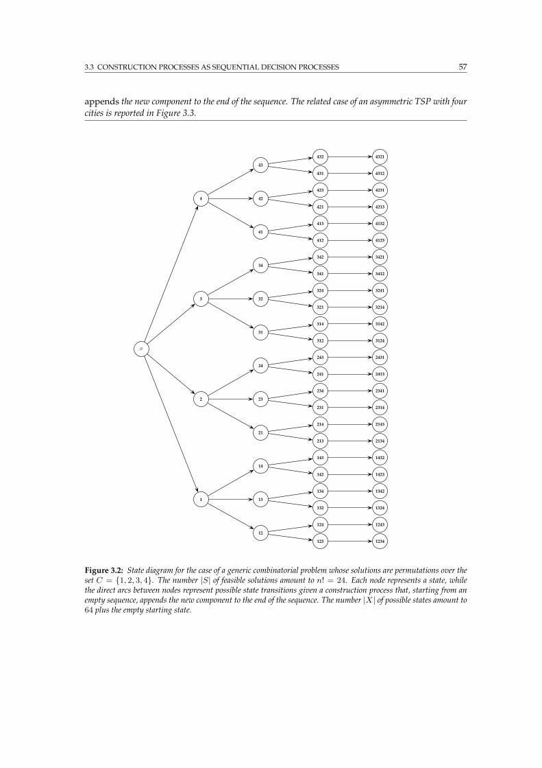
3.3 CONSTRUCTION PROCESSES AS SEQUENTIAL DECISION PROCESSES 57
appends the new component to the end of the sequence. The related case of an asymmetric TSP with four
cities is reported in Figure 3.3.
∅
1
2
3
4
12
13
14
21
23
24
31
32
34
41
42
43
123
124
132
134
142
143
1234
1243
1324
1342
1423
1432
213
214
231
234
241
243
2134
2143
2314
2341
2413
2431
312
314
321
324
341
342
3124
3142
3214
3241
3412
3421
412
413
421
423
431
432
4123
4132
4213
4231
4312
4321
Figure 3.2: State diagram for the case of a generic combinatorial problem whose solutions are permutations over theset C = 1, 2, 3, 4. The number |S| of feasible solutions amount to n! = 24. Each node represents a state, whilethe direct arcs between nodes represent possible state transitions given a construction process that, starting from anempty sequence, appends the new component to the end of the sequence. The number |X| of possible states amount to64 plus the empty starting state.
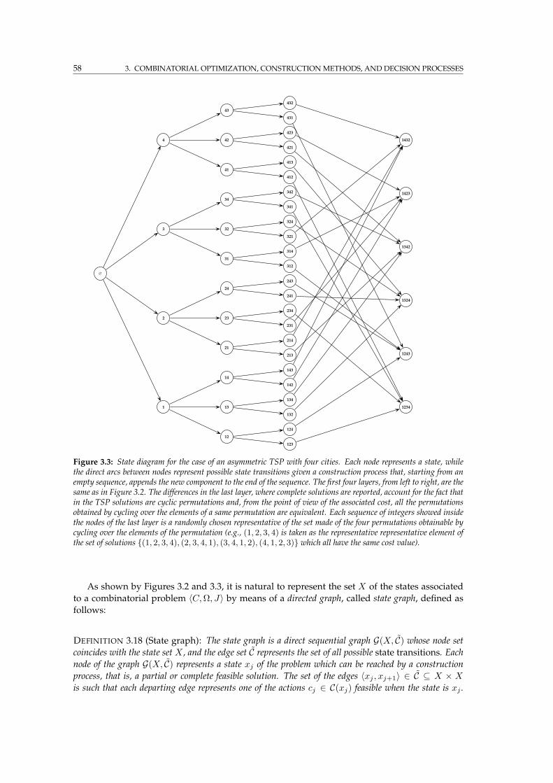
58 3. COMBINATORIAL OPTIMIZATION, CONSTRUCTIONMETHODS, AND DECISION PROCESSES
∅
1
2
3
4
12
13
14
21
23
24
31
32
34
41
42
43
123
124
132
134
142
143
1234
1243
1324
1342
1423
1432
213
214
231
234
241
243
312
314
321
324
341
342
412
413
421
423
431
432
Figure 3.3: State diagram for the case of an asymmetric TSP with four cities. Each node represents a state, whilethe direct arcs between nodes represent possible state transitions given a construction process that, starting from anempty sequence, appends the new component to the end of the sequence. The first four layers, from left to right, are thesame as in Figure 3.2. The differences in the last layer, where complete solutions are reported, account for the fact thatin the TSP solutions are cyclic permutations and, from the point of view of the associated cost, all the permutationsobtained by cycling over the elements of a same permutation are equivalent. Each sequence of integers showed insidethe nodes of the last layer is a randomly chosen representative of the set made of the four permutations obtainable bycycling over the elements of the permutation (e.g., (1, 2, 3, 4) is taken as the representative representative element ofthe set of solutions (1, 2, 3, 4), (2, 3, 4, 1), (3, 4, 1, 2), (4, 1, 2, 3) which all have the same cost value).
As shown by Figures 3.2 and 3.3, it is natural to represent the set X of the states associated
to a combinatorial problem 〈C,Ω, J〉 by means of a directed graph, called state graph, defined as
follows:
DEFINITION 3.18 (State graph): The state graph is a direct sequential graph G(X, C) whose node setcoincides with the state set X , and the edge set C represents the set of all possible state transitions. Eachnode of the graph G(X, C) represents a state xj of the problem which can be reached by a construction
process, that is, a partial or complete feasible solution. The set of the edges 〈xj , xj+1〉 ∈ C ⊆ X × Xis such that each departing edge represents one of the actions cj ∈ C(xj) feasible when the state is xj .
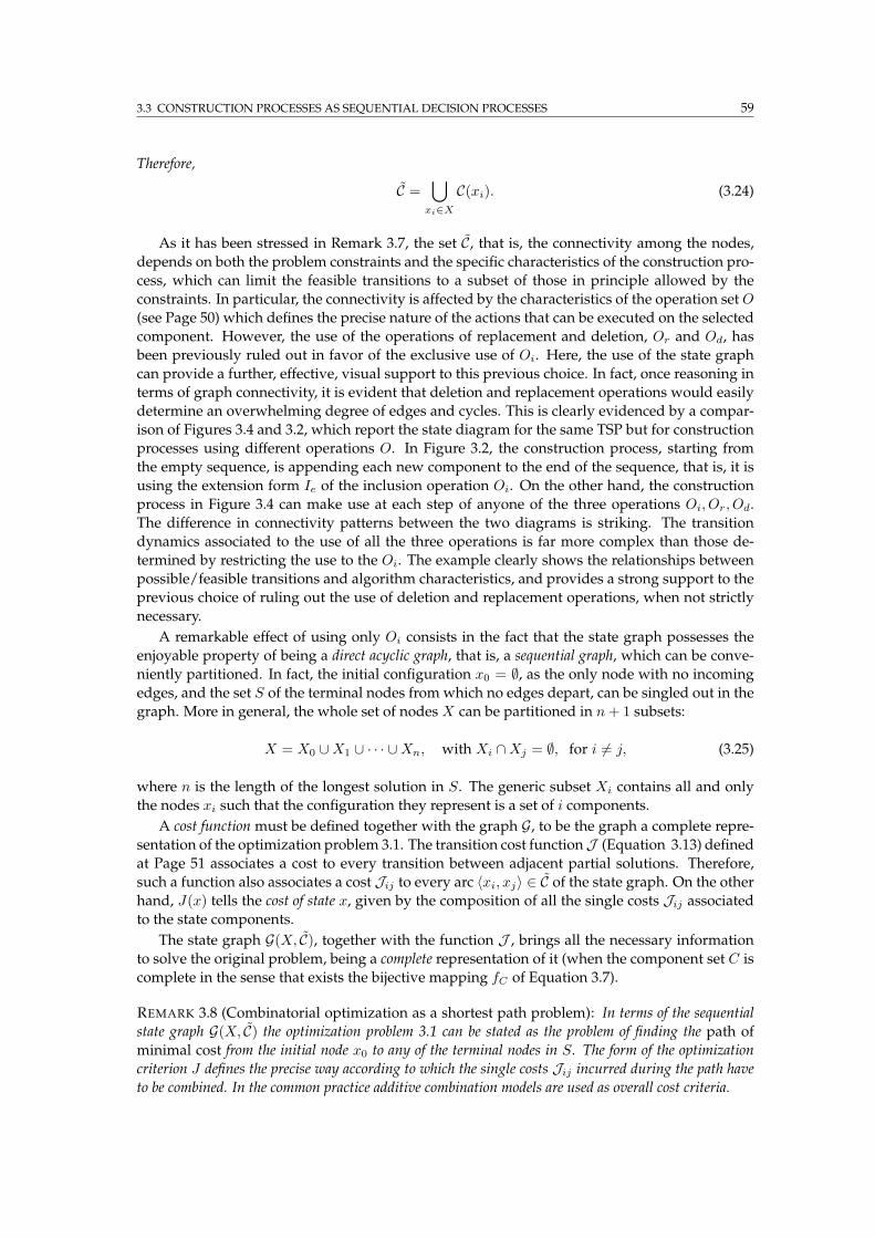
3.3 CONSTRUCTION PROCESSES AS SEQUENTIAL DECISION PROCESSES 59
Therefore,
C =⋃
xi∈X
C(xi). (3.24)
As it has been stressed in Remark 3.7, the set C, that is, the connectivity among the nodes,
depends on both the problem constraints and the specific characteristics of the construction pro-
cess, which can limit the feasible transitions to a subset of those in principle allowed by the
constraints. In particular, the connectivity is affected by the characteristics of the operation setO
(see Page 50) which defines the precise nature of the actions that can be executed on the selected
component. However, the use of the operations of replacement and deletion, Or and Od, has
been previously ruled out in favor of the exclusive use of Oi. Here, the use of the state graph
can provide a further, effective, visual support to this previous choice. In fact, once reasoning in
terms of graph connectivity, it is evident that deletion and replacement operations would easily
determine an overwhelming degree of edges and cycles. This is clearly evidenced by a compar-
ison of Figures 3.4 and 3.2, which report the state diagram for the same TSP but for construction
processes using different operations O. In Figure 3.2, the construction process, starting from
the empty sequence, is appending each new component to the end of the sequence, that is, it is
using the extension form Ie of the inclusion operation Oi. On the other hand, the construction
process in Figure 3.4 can make use at each step of anyone of the three operations Oi, Or, Od.
The difference in connectivity patterns between the two diagrams is striking. The transition
dynamics associated to the use of all the three operations is far more complex than those de-
termined by restricting the use to the Oi. The example clearly shows the relationships between
possible/feasible transitions and algorithm characteristics, and provides a strong support to the
previous choice of ruling out the use of deletion and replacement operations, when not strictly
necessary.
A remarkable effect of using only Oi consists in the fact that the state graph possesses the
enjoyable property of being a direct acyclic graph, that is, a sequential graph, which can be conve-
niently partitioned. In fact, the initial configuration x0 = ∅, as the only node with no incoming
edges, and the set S of the terminal nodes from which no edges depart, can be singled out in the
graph. More in general, the whole set of nodes X can be partitioned in n+ 1 subsets:
X = X0 ∪X1 ∪ · · · ∪Xn, with Xi ∩Xj = ∅, for i 6= j, (3.25)
where n is the length of the longest solution in S. The generic subset Xi contains all and only
the nodes xi such that the configuration they represent is a set of i components.
A cost function must be defined together with the graph G, to be the graph a complete repre-
sentation of the optimization problem 3.1. The transition cost functionJ (Equation 3.13) defined
at Page 51 associates a cost to every transition between adjacent partial solutions. Therefore,
such a function also associates a cost Jij to every arc 〈xi, xj〉 ∈ C of the state graph. On the other
hand, J(x) tells the cost of state x, given by the composition of all the single costs Jij associatedto the state components.
The state graph G(X, C), together with the function J , brings all the necessary information
to solve the original problem, being a complete representation of it (when the component set C is
complete in the sense that exists the bijective mapping fC of Equation 3.7).
REMARK 3.8 (Combinatorial optimization as a shortest path problem): In terms of the sequential
state graph G(X, C) the optimization problem 3.1 can be stated as the problem of finding the path of
minimal cost from the initial node x0 to any of the terminal nodes in S. The form of the optimization
criterion J defines the precise way according to which the single costs Jij incurred during the path have
to be combined. In the common practice additive combination models are used as overall cost criteria.
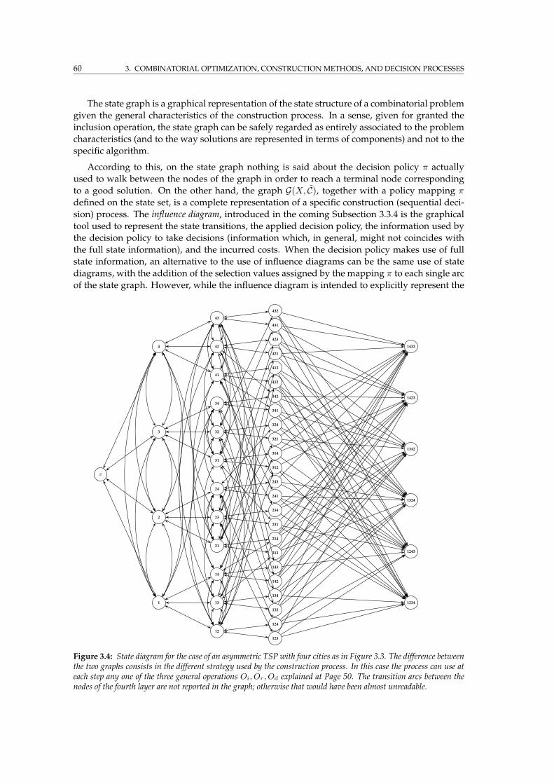
60 3. COMBINATORIAL OPTIMIZATION, CONSTRUCTIONMETHODS, AND DECISION PROCESSES
The state graph is a graphical representation of the state structure of a combinatorial problem
given the general characteristics of the construction process. In a sense, given for granted the
inclusion operation, the state graph can be safely regarded as entirely associated to the problem
characteristics (and to the way solutions are represented in terms of components) and not to the
specific algorithm.
According to this, on the state graph nothing is said about the decision policy π actually
used to walk between the nodes of the graph in order to reach a terminal node corresponding
to a good solution. On the other hand, the graph G(X, C), together with a policy mapping π
defined on the state set, is a complete representation of a specific construction (sequential deci-
sion) process. The influence diagram, introduced in the coming Subsection 3.3.4 is the graphical
tool used to represent the state transitions, the applied decision policy, the information used by
the decision policy to take decisions (information which, in general, might not coincides with
the full state information), and the incurred costs. When the decision policy makes use of full
state information, an alternative to the use of influence diagrams can be the same use of state
diagrams, with the addition of the selection values assigned by the mapping π to each single arc
of the state graph. However, while the influence diagram is intended to explicitly represent the
∅
1
2
3
4
12
13
14
21
23
24
31
32
34
41
42
43
123
124
132
134
142
143
1234
1243
1324
1342
1423
1432
213
214
231
234
241
243
312
314
321
324
341
342
412
413
421
423
431
432
Figure 3.4: State diagram for the case of an asymmetric TSP with four cities as in Figure 3.3. The difference betweenthe two graphs consists in the different strategy used by the construction process. In this case the process can use ateach step any one of the three general operations Oi, Or, Od explained at Page 50. The transition arcs between thenodes of the fourth layer are not reported in the graph; otherwise that would have been almost unreadable.
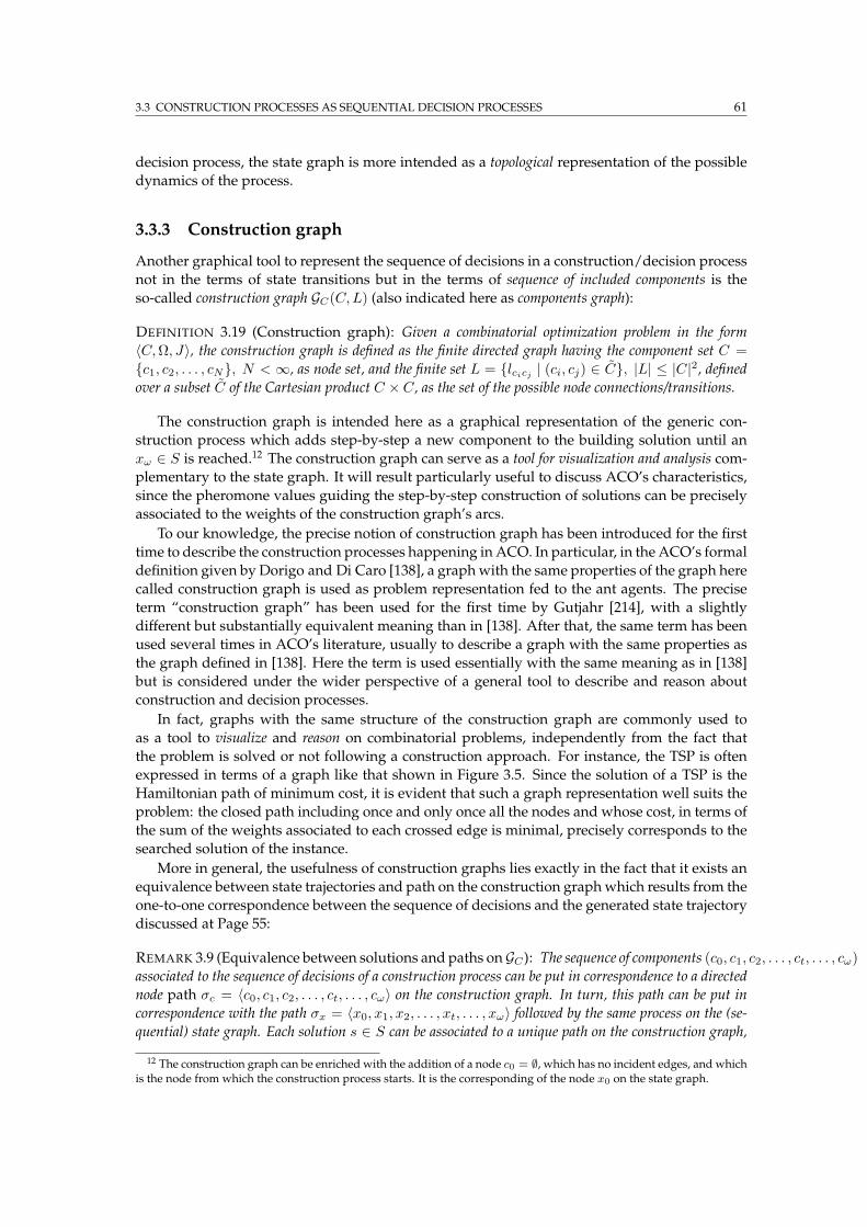
3.3 CONSTRUCTION PROCESSES AS SEQUENTIAL DECISION PROCESSES 61
decision process, the state graph is more intended as a topological representation of the possible
dynamics of the process.
3.3.3 Construction graph
Another graphical tool to represent the sequence of decisions in a construction/decision process
not in the terms of state transitions but in the terms of sequence of included components is the
so-called construction graph GC(C,L) (also indicated here as components graph):
DEFINITION 3.19 (Construction graph): Given a combinatorial optimization problem in the form
〈C,Ω, J〉, the construction graph is defined as the finite directed graph having the component set C =
c1, c2, . . . , cN, N < ∞, as node set, and the finite set L = lcicj| (ci, cj) ∈ C, |L| ≤ |C|2, defined
over a subset C of the Cartesian product C × C, as the set of the possible node connections/transitions.
The construction graph is intended here as a graphical representation of the generic con-
struction process which adds step-by-step a new component to the building solution until an
xω ∈ S is reached.12 The construction graph can serve as a tool for visualization and analysis com-
plementary to the state graph. It will result particularly useful to discuss ACO’s characteristics,
since the pheromone values guiding the step-by-step construction of solutions can be precisely
associated to the weights of the construction graph’s arcs.
To our knowledge, the precise notion of construction graph has been introduced for the first
time to describe the construction processes happening in ACO. In particular, in the ACO’s formal
definition given by Dorigo and Di Caro [138], a graphwith the same properties of the graph here
called construction graph is used as problem representation fed to the ant agents. The precise
term “construction graph” has been used for the first time by Gutjahr [214], with a slightly
different but substantially equivalent meaning than in [138]. After that, the same term has been
used several times in ACO’s literature, usually to describe a graph with the same properties as
the graph defined in [138]. Here the term is used essentially with the same meaning as in [138]
but is considered under the wider perspective of a general tool to describe and reason about
construction and decision processes.
In fact, graphs with the same structure of the construction graph are commonly used to
as a tool to visualize and reason on combinatorial problems, independently from the fact that
the problem is solved or not following a construction approach. For instance, the TSP is often
expressed in terms of a graph like that shown in Figure 3.5. Since the solution of a TSP is the
Hamiltonian path of minimum cost, it is evident that such a graph representation well suits the
problem: the closed path including once and only once all the nodes and whose cost, in terms of
the sum of the weights associated to each crossed edge is minimal, precisely corresponds to the
searched solution of the instance.
More in general, the usefulness of construction graphs lies exactly in the fact that it exists an
equivalence between state trajectories and path on the construction graphwhich results from the
one-to-one correspondence between the sequence of decisions and the generated state trajectory
discussed at Page 55:
REMARK 3.9 (Equivalence between solutions and paths on GC): The sequence of components (c0, c1, c2, . . . , ct, . . . , cω)
associated to the sequence of decisions of a construction process can be put in correspondence to a directed
node path σc = 〈c0, c1, c2, . . . , ct, . . . , cω〉 on the construction graph. In turn, this path can be put in
correspondence with the path σx = 〈x0, x1, x2, . . . , xt, . . . , xω〉 followed by the same process on the (se-
quential) state graph. Each solution s ∈ S can be associated to a unique path on the construction graph,
12 The construction graph can be enriched with the addition of a node c0 = ∅, which has no incident edges, and whichis the node from which the construction process starts. It is the corresponding of the node x0 on the state graph.
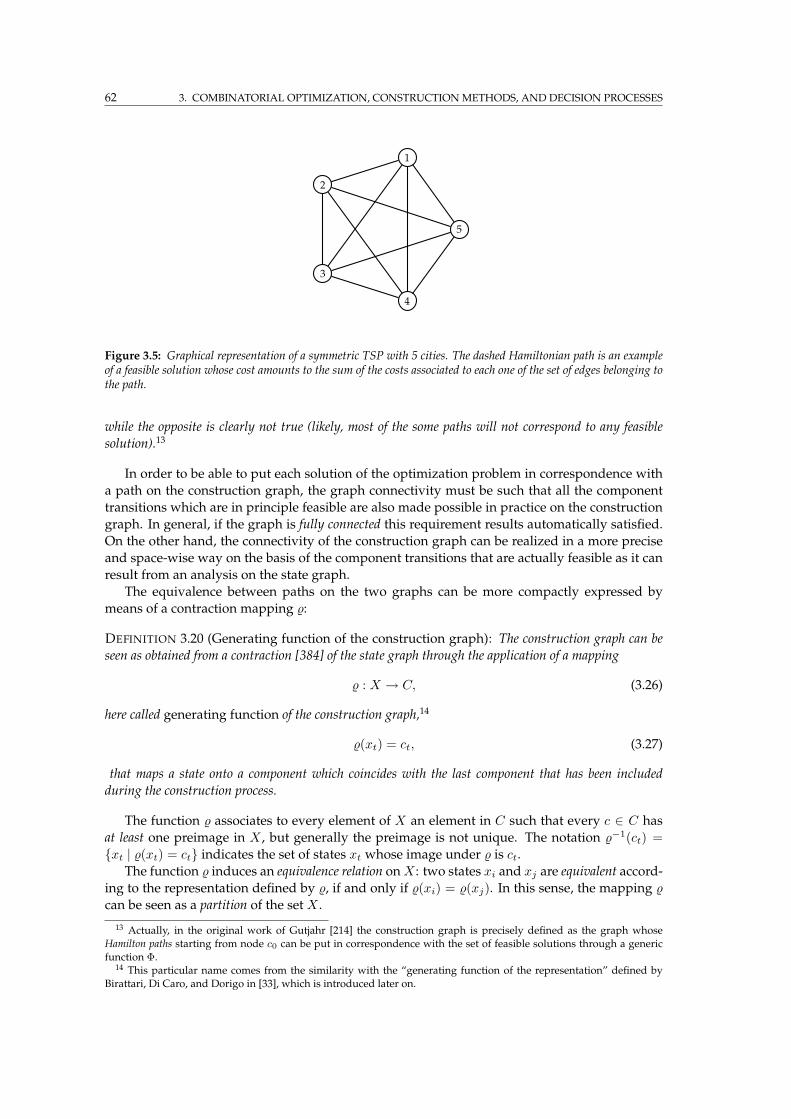
62 3. COMBINATORIAL OPTIMIZATION, CONSTRUCTIONMETHODS, AND DECISION PROCESSES
1
2
3
4
5
Figure 3.5: Graphical representation of a symmetric TSP with 5 cities. The dashed Hamiltonian path is an exampleof a feasible solution whose cost amounts to the sum of the costs associated to each one of the set of edges belonging tothe path.
while the opposite is clearly not true (likely, most of the some paths will not correspond to any feasible
solution).13
In order to be able to put each solution of the optimization problem in correspondence with
a path on the construction graph, the graph connectivity must be such that all the component
transitions which are in principle feasible are also made possible in practice on the construction
graph. In general, if the graph is fully connected this requirement results automatically satisfied.
On the other hand, the connectivity of the construction graph can be realized in a more precise
and space-wise way on the basis of the component transitions that are actually feasible as it can
result from an analysis on the state graph.
The equivalence between paths on the two graphs can be more compactly expressed by
means of a contraction mapping :
DEFINITION 3.20 (Generating function of the construction graph): The construction graph can be
seen as obtained from a contraction [384] of the state graph through the application of a mapping
: X → C, (3.26)
here called generating function of the construction graph,14
(xt) = ct, (3.27)
that maps a state onto a component which coincides with the last component that has been included
during the construction process.
The function associates to every element of X an element in C such that every c ∈ C has
at least one preimage in X , but generally the preimage is not unique. The notation −1(ct) =
xt | (xt) = ct indicates the set of states xt whose image under is ct.
The function induces an equivalence relation onX : two states xi and xj are equivalent accord-
ing to the representation defined by , if and only if (xi) = (xj). In this sense, the mapping
can be seen as a partition of the set X .
13 Actually, in the original work of Gutjahr [214] the construction graph is precisely defined as the graph whoseHamilton paths starting from node c0 can be put in correspondence with the set of feasible solutions through a genericfunction Φ.
14 This particular name comes from the similarity with the “generating function of the representation” defined byBirattari, Di Caro, and Dorigo in [33], which is introduced later on.
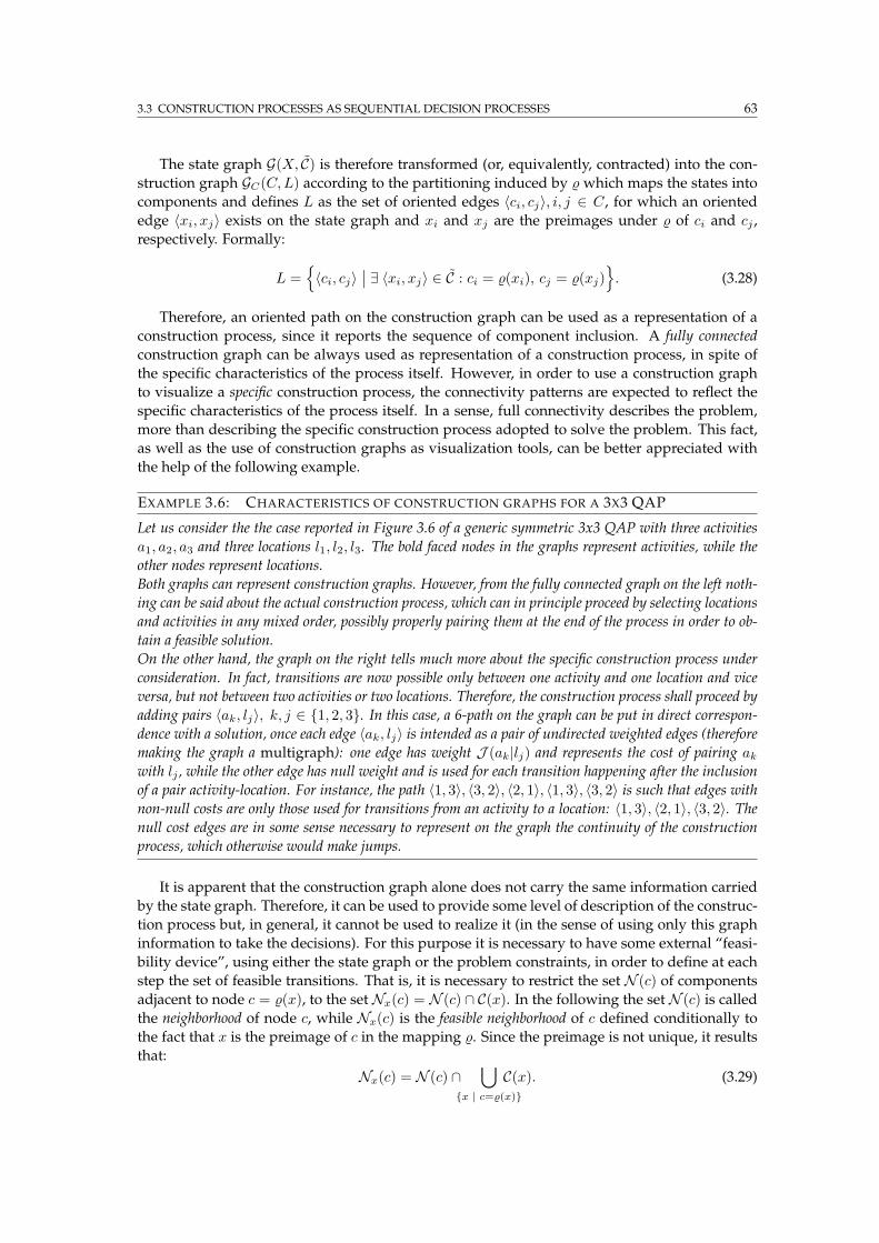
3.3 CONSTRUCTION PROCESSES AS SEQUENTIAL DECISION PROCESSES 63
The state graph G(X, C) is therefore transformed (or, equivalently, contracted) into the con-
struction graph GC(C,L) according to the partitioning induced by which maps the states into
components and defines L as the set of oriented edges 〈ci, cj〉, i, j ∈ C, for which an oriented
edge 〈xi, xj〉 exists on the state graph and xi and xj are the preimages under of ci and cj ,
respectively. Formally:
L =
〈ci, cj〉∣
∣ ∃ 〈xi, xj〉 ∈ C : ci = (xi), cj = (xj)
. (3.28)
Therefore, an oriented path on the construction graph can be used as a representation of a
construction process, since it reports the sequence of component inclusion. A fully connected
construction graph can be always used as representation of a construction process, in spite of
the specific characteristics of the process itself. However, in order to use a construction graph
to visualize a specific construction process, the connectivity patterns are expected to reflect the
specific characteristics of the process itself. In a sense, full connectivity describes the problem,
more than describing the specific construction process adopted to solve the problem. This fact,
as well as the use of construction graphs as visualization tools, can be better appreciated with
the help of the following example.
EXAMPLE 3.6: CHARACTERISTICS OF CONSTRUCTION GRAPHS FOR A 3X3 QAP
Let us consider the the case reported in Figure 3.6 of a generic symmetric 3x3 QAP with three activities
a1, a2, a3 and three locations l1, l2, l3. The bold faced nodes in the graphs represent activities, while the
other nodes represent locations.
Both graphs can represent construction graphs. However, from the fully connected graph on the left noth-
ing can be said about the actual construction process, which can in principle proceed by selecting locations
and activities in any mixed order, possibly properly pairing them at the end of the process in order to ob-
tain a feasible solution.
On the other hand, the graph on the right tells much more about the specific construction process under
consideration. In fact, transitions are now possible only between one activity and one location and vice
versa, but not between two activities or two locations. Therefore, the construction process shall proceed by
adding pairs 〈ak, lj〉, k, j ∈ 1, 2, 3. In this case, a 6-path on the graph can be put in direct correspon-
dence with a solution, once each edge 〈ak, lj〉 is intended as a pair of undirected weighted edges (thereforemaking the graph a multigraph): one edge has weight J (ak|lj) and represents the cost of pairing akwith lj , while the other edge has null weight and is used for each transition happening after the inclusion
of a pair activity-location. For instance, the path 〈1, 3〉, 〈3, 2〉, 〈2, 1〉, 〈1, 3〉, 〈3, 2〉 is such that edges with
non-null costs are only those used for transitions from an activity to a location: 〈1, 3〉, 〈2, 1〉, 〈3, 2〉. Thenull cost edges are in some sense necessary to represent on the graph the continuity of the construction
process, which otherwise would make jumps.
It is apparent that the construction graph alone does not carry the same information carried
by the state graph. Therefore, it can be used to provide some level of description of the construc-
tion process but, in general, it cannot be used to realize it (in the sense of using only this graph
information to take the decisions). For this purpose it is necessary to have some external “feasi-
bility device”, using either the state graph or the problem constraints, in order to define at each
step the set of feasible transitions. That is, it is necessary to restrict the set N (c) of components
adjacent to node c = (x), to the set Nx(c) = N (c) ∩ C(x). In the following the set N (c) is called
the neighborhood of node c, while Nx(c) is the feasible neighborhood of c defined conditionally to
the fact that x is the preimage of c in the mapping . Since the preimage is not unique, it results
that:
Nx(c) = N (c) ∩⋃
x | c=(x)
C(x). (3.29)
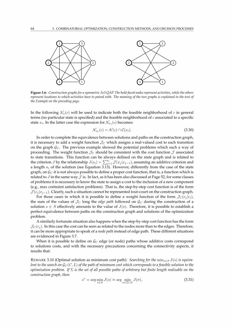
64 3. COMBINATORIAL OPTIMIZATION, CONSTRUCTIONMETHODS, AND DECISION PROCESSES
1
2
3 1
2
3 1
2
3 1
2
3
Figure 3.6: Construction graphs for a symmetric 3x3 QAP. The bold-faced nodes represent activities, while the othersrepresent locations to which activities have to paired with. The meaning of the two graphs is explained in the text ofthe Example on the preceding page.
In the following Nx(c) will be used to indicate both the feasible neighborhood of c in general
terms (no particular state is specified) and the feasible neighborhood of c associated to a specific
state xt. In the latter case the expression for Nxt(c) becomes:
Nxt(c) = N (c) ∩ C(xt). (3.30)
In order to complete the equivalence between solutions and paths on the construction graph,
it is necessary to add a weight function JC which assigns a real-valued cost to each transition
on the graph GC . The previous example showed the potential problems which such a way of
proceeding. The weight function JC should be consistent with the cost function J associated
to state transitions. This function can be always defined on the state graph and is related to
the criterion J by the relationship J(si) =∑ni
j=1 J (xj |xj−1), assuming an additive criterion and
a length ni of the solution (see Equation 3.13). However, differently from the case of the state
graph, on GC it is not always possible to define a proper cost function, that is, a function which is
related to J in the samewayJ is. In fact, as it has been also discussed at Page 52, for some classes
of problems it is necessary to know the state to assign a cost to the inclusion of a new component
(e.g., max contraint satisfaction problems). That is, the step-by-step cost function is of the form
J (cj |xj−1). Clearly, such a situation cannot be represented tout-court on the construction graph.
For those cases in which it is possible to define a weight function of the form JC(cj |ci),the sum of the values of JC long the edge path followed on GC during the construction of a
solution s ∈ S effectively amounts to the value of J(s). Therefore, it is possible to establish a
perfect equivalence between paths on the construction graph and solutions of the optimization
problem.
A similarly fortunate situation also happens when the step-by-step cost function has the form
JC(cj). In this case the cost can be seen as related to the nodes more than to the edges. Therefore,
it can be more appropriate to speak of a node path instead of edge path. These different situations
are evidenced in Figure 3.7.
When it is possible to define on GC edge (or node) paths whose additive costs correspond
to solutions costs, and with the necessary precautions concerning the connectivity aspects, it
results that:
REMARK 3.10 (Optimal solution as minimum cost path): Searching for the mins∈S J(s) is equiva-
lent to the search on GC(C,L) of the path of minimum cost which corresponds to a feasible solution to the
optimization problem. If Σ is the set of all possible paths of arbitrary but finite length realizable on the
construction graph, then:
s∗ = arg mins∈S
J(s) ≡ arg minσ∈Σ∩S
J(σ), (3.31)
3.3 CONSTRUCTION PROCESSES AS SEQUENTIAL DECISION PROCESSES 65
1 2
3 4
J (2|1)
J (4|1)
J (3|1) J (4|2)
J (3|2)
J (4|3)
1 2
3 4 J (4)J (3)
J (1) J (2) 1 2
3 4
J (2)
J (1)
J (1)
J (1) J (2)J (2)
Figure 3.7: Different ways of mapping problem costs on the construction graph. The first graph from the left is anexample of a problem (e.g., TSP) in which costs can be defined as J (ci|cj), that is, they can be associated to edges〈ci, cj〉 on the construction graph. In the reported case costs are symmetric. The bold-faced elements in all the threegraphs indicate where the costs are mapped onto. The middle graph refers to a problem in which costs are associatedto the inclusion of the single component ci, independently from the actual state (e.g., knapsack problems). Therefore,costs are in the form J (ci) and can be associated to each node ci of the construction graph. The last graph to the rightis the equivalent of the middle one but shows how the same result of associating costs to the nodes can be obtained byassociating costs to edges of the graph. Costs are reported only for nodes 1 and 2, while bold-faced edges refers to node1 only. Every node ci has a pair of input/output edges. The edge 〈ci, cj〉, has associated a weight equal to J (cj),while the opposite one has a weight equal to J (ci). That is, all the incident edges to a node ci have a weight equal toJ (ci). In this way every node transition to ci incurs in the same cost ci, which is in practice the cost to include thecomponent ci independently from the previous component or state. Therefore, it is always possible to reason in termsof edge path, with costs associated to the edge weights.
where the notation has been a bit abused, intending with Σ ∩ S the subsets of the path set Σ
which correspond to feasible solutions, and with J(σ) the evaluation of the path itself according
to the sum of the single cost contributions either in the form JC(ci+1|ci) or JC(ci+1).
Domains of application of the construction graph
From the discussions so far, it is apparent that the construction graph can be a particularly ap-
propriate tool to reason on construction processes applied to problems whose solutions are nat-
urally expressed in terms of sequences (e.g., TSP) and when the process inclusion operation is
the extension one Ie. In fact, in these cases, the construction graph is a faithful representation
of the process and solutions can be directly associated to paths. The cost of inclusion of a new
component cj conditioned to the fact that ci is the last included one, is usually well defined in
these cases. More in general, the transition clast → cnew, which is exactly the one reported on
the construction graph, can be seen as playing a special role (e.g., in greedy methods for TSP
is common to select the new city as the one which is “closest” to the one last included in the
sequence). That is:
REMARK 3.11: The construction graph appears as well suited to represent processes for which the notion
of pair of components, or equivalently, of transition between components, plays a sort of privileged
role. It will be shown in the next chapter that this is precisely the case of ACO.
Also in the cases of set problems (e.g., the knapsack problem), in which the cost is associated
to each single included component independently from the state, the path on the construction
graph can be effectively used to represent solutions. In these cases the cost of the solution can
be evaluated either in terms of costs associated to each single node or costs associated to node
transitions (as it has been shown on the two rightmost graphs of Figure 3.7).
On the other side, when for example the insertion operation Ii is used, this is not anymore
true. The followed path cannot be directly associated to the solution actually constructed since
all the already included components can play the role of being the one next to which the newly
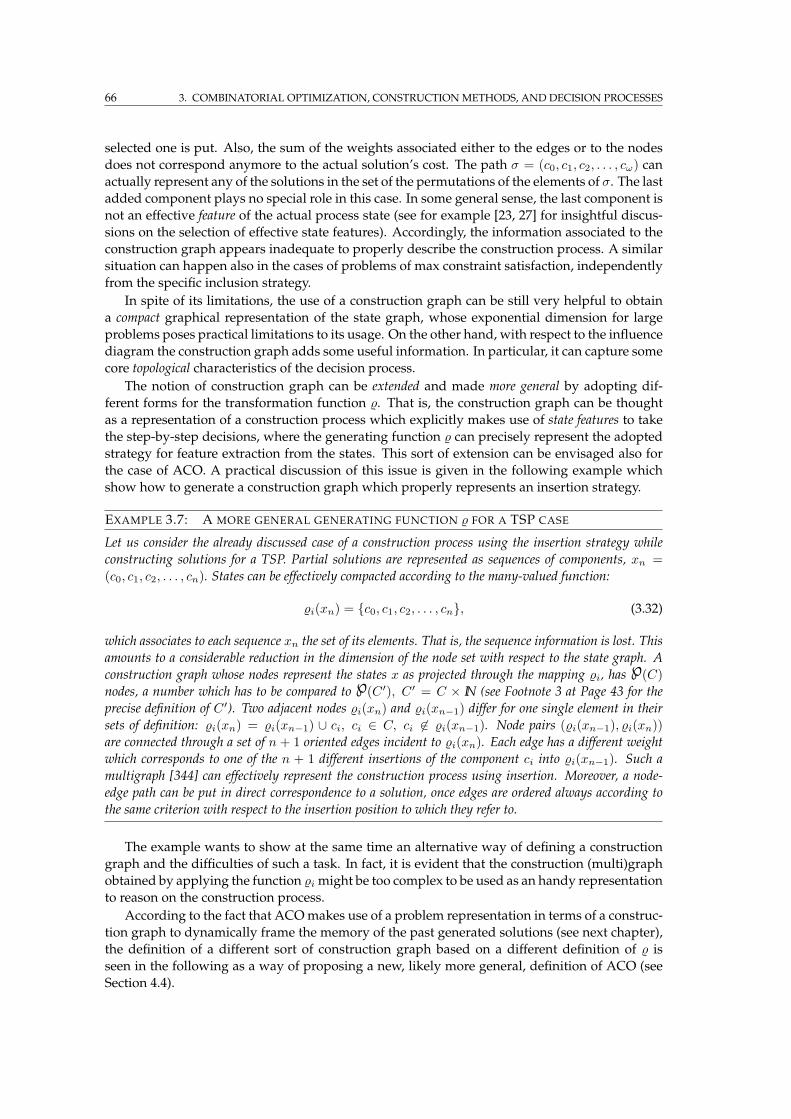
66 3. COMBINATORIAL OPTIMIZATION, CONSTRUCTIONMETHODS, AND DECISION PROCESSES
selected one is put. Also, the sum of the weights associated either to the edges or to the nodes
does not correspond anymore to the actual solution’s cost. The path σ = (c0, c1, c2, . . . , cω) can
actually represent any of the solutions in the set of the permutations of the elements of σ. The last
added component plays no special role in this case. In some general sense, the last component is
not an effective feature of the actual process state (see for example [23, 27] for insightful discus-
sions on the selection of effective state features). Accordingly, the information associated to the
construction graph appears inadequate to properly describe the construction process. A similar
situation can happen also in the cases of problems of max constraint satisfaction, independently
from the specific inclusion strategy.
In spite of its limitations, the use of a construction graph can be still very helpful to obtain
a compact graphical representation of the state graph, whose exponential dimension for large
problems poses practical limitations to its usage. On the other hand, with respect to the influence
diagram the construction graph adds some useful information. In particular, it can capture some
core topological characteristics of the decision process.
The notion of construction graph can be extended and made more general by adopting dif-
ferent forms for the transformation function . That is, the construction graph can be thought
as a representation of a construction process which explicitly makes use of state features to take
the step-by-step decisions, where the generating function can precisely represent the adopted
strategy for feature extraction from the states. This sort of extension can be envisaged also for
the case of ACO. A practical discussion of this issue is given in the following example which
show how to generate a construction graph which properly represents an insertion strategy.
EXAMPLE 3.7: A MORE GENERAL GENERATING FUNCTION FOR A TSP CASE
Let us consider the already discussed case of a construction process using the insertion strategy while
constructing solutions for a TSP. Partial solutions are represented as sequences of components, xn =
(c0, c1, c2, . . . , cn). States can be effectively compacted according to the many-valued function:
i(xn) = c0, c1, c2, . . . , cn, (3.32)
which associates to each sequence xn the set of its elements. That is, the sequence information is lost. This
amounts to a considerable reduction in the dimension of the node set with respect to the state graph. A
construction graph whose nodes represent the states x as projected through the mapping i, has ℘(C)
nodes, a number which has to be compared to ℘(C ′), C ′ = C × IN (see Footnote 3 at Page 43 for the
precise definition of C ′). Two adjacent nodes i(xn) and i(xn−1) differ for one single element in their
sets of definition: i(xn) = i(xn−1) ∪ ci, ci ∈ C, ci 6∈ i(xn−1). Node pairs (i(xn−1), i(xn))
are connected through a set of n + 1 oriented edges incident to i(xn). Each edge has a different weight
which corresponds to one of the n + 1 different insertions of the component ci into i(xn−1). Such a
multigraph [344] can effectively represent the construction process using insertion. Moreover, a node-
edge path can be put in direct correspondence to a solution, once edges are ordered always according to
the same criterion with respect to the insertion position to which they refer to.
The example wants to show at the same time an alternative way of defining a construction
graph and the difficulties of such a task. In fact, it is evident that the construction (multi)graph
obtained by applying the function imight be too complex to be used as an handy representation
to reason on the construction process.
According to the fact that ACOmakes use of a problem representation in terms of a construc-
tion graph to dynamically frame the memory of the past generated solutions (see next chapter),
the definition of a different sort of construction graph based on a different definition of is
seen in the following as a way of proposing a new, likely more general, definition of ACO (see
Section 4.4).
3.3 CONSTRUCTION PROCESSES AS SEQUENTIAL DECISION PROCESSES 67
3.3.4 The general framework of Markov decision processes
From the previous definitions and discussions on the concept of state, it is apparent that at each
node xj ∈ X of the state graph G(X, C) the only information that is necessary to determine
feasible actions and the future cost of a whatever path bringing to a terminal node is actually
the knowledge of the current state xt and of its cost J(xj). That is, in more general terms,
the path followed from x0 to xj does not matter for what concerns the future: the information
associated to xj summarizes all the necessary information. This is the property that informally
characterizes the same concept of state as defined in Subsection 3.3.1. Since what is known in
the literature as Markov property [367, Chapter 4] is precisely related to the concept of state, it is
clear that the state, when correctly conceived, is always a state in the Markov sense. Accordingly,
when described in terms of its state, any discrete-time system is intrinsically Markov.15 16
According to this equivalence, the state description of a process can be reformulated in the
terms of a Markov chain. In particular, the arcs in the state graph representation can be more in
general thought as representing probabilistic state transitions: every possible state transition can
happen with a certain probability value which is associated to the arc. The deterministic case
considered in this thesis can be seen as a limit case of the probabilistic one. More in general, the
state graph can be associated to the structure of a generic Markov decision process (MDP), that is,
a Markov chain generated by explicitly issuing control actions at the states [229, 353].17
An MDP is a basic modeling framework for sequential decision processes. In a broad sense,
it is the main framework of reference for decision making. The range of interest of MDPs is
much wider than that of the ACO framework, but it is useful to reason about ACO referring
also to the modeling tools, the language, and the algorithms proper of the MDP field. In fact,
this will help to make clearer which are the specificities of the decision problems faced by ACO,
as well as the theoretical properties and limitations implicit in the ACO’s design. An indirect
confirmation of the usefulness of using such a language comes from the fact that the first proof
of convergence to optimality for ACO algorithms, given by Gutjahr in [214], precisely made use
of the notion of MDPs (actually, also other subsequent convergence proofs and discussions from
the same author [215, 216]) make use of the same notion).
A Markov decision process is a controlled stochastic process that: (i) assumes that every
process state depends only on the previous process state and not on the history of previous
states (Markov assumption), (ii) assigns costs (or rewards) to state transitions.18 More formally,
an MDP is finite state automaton with a state-transition feedback function described by the 4-
tuple 〈X,U, T,J 〉where:
• X is a finite set of problem states, representing the environment;
• U is a finite set of actions;
• T : X×U×X → [0, 1] defines the transition probability distributionP (xi|xj , uk) that describesthe effect of actions on the world state;
15 Birattari, Di Caro, and Dorigo [34, Page 192] give a detailed mathematical proof of this intuitive equivalence in thegeneral case of a stochastic discrete-time system.
16 The often found expressions like Markov order n-th, have to be seen as a way of dealing with systems whose properstate can be encoded by retaining information from the last n decision steps, but it is in practice more convenient to focuson the single decision step and make explicit from how many steps information has to be maintained in order to build aproper state.
17 Probabilistic transitions mean the following situation. If N (xj) = x1j+1
, x2j+1
, . . . , xkj+1
is the set of states
reachable from xj in one step, then, after issuing at state xj the control action uj , the state xij+1
∈ N (xj) will be the
next state with a probability equal to P (xij+1
|xj , uj).18 In the following, consistently with the terminology used so far, which refers to minimization problems, only cost
models are considered. The case for rewards would refer to maximization problems.
68 3. COMBINATORIAL OPTIMIZATION, CONSTRUCTIONMETHODS, AND DECISION PROCESSES
• J : X × U × X → IR defines a cost model that describes costs associated with a state
transition under some action.
Usually, once a Markov model is defined for the system under study, the aim is to exploit the
characteristics of the model to either search for the optimal action policy π∗ or to study the
dynamics of the system under an assigned policy π (e.g., probability of reaching each terminal
state, asymptotic state occupancies). In general, solving anMDPmeans to compute either: (i) the
policy π∗ which minimizes the overall expected cost incurred when starting from one specific
state, or, (ii) the policy π∗ which minimizes for all the states the overall expected cost incurred
when starting from a state sampled over the whole state set according to an assigned probability
distribution, or, (iii) the overall expected cost, as in (i) or (ii), but for a specific assigned policy
π. For a Markov chain the objectives are similar, except for the fact that the system can only be
observed and not directly controlled.
When all the aspects defining the MDP at hand are precisely known and the cost model is
additive, the methods of dynamic programming, and in particular value iteration and policy itera-
tion, described in Subsection 3.4.2, are among the most common and effectice ways of dealing
with MDP solution. When this is not the case (e.g, the characteristics of the Markov environ-
ment are not fully known in advance), other techniques must be be used, like for instance A∗
algorithms [336] (that address the situation in which the goal states are not known in advance),
or those algorithms developed in the field of reinforcement learning (e.g., Q-learning [442, 414]),
which address both the problem of the complete lack of the environment model and that of
delayed rewards (which cannot be dealt efficiently by dynamic programming).
The literature on Markov processes is extensive. The textbook [353] contains a detailed and
quite comprehensive presentation of the subject. In Appendix C a short overview on the charac-
teristics and properties of Markov decision processes and partially observable Markov decision
processes is given. The discussion has focused on the general case of a stochastic model for
state transitions, even if in the class of combinatorial problems meant to be solved by ACO state
transitions are supposed to be strictly deterministic.
Graphical representations for MDPs
The most informative graphical way used to represent the dynamics of an MDP, and, more in
general of a decision process, is an influence diagram [229], which reports all the information
related to the followed trajectory in the state space of the process. The influence diagram is
complementary to the state diagram, which shows the general connectivity among the states,
and the transition graph, which has a node for each state and an action node for each state-
action pair, with the action node positioned on the arc connecting the two end-states. Basically,
the transition graph reduces to the state graph in the deterministic case since for each issued
action only one specific state transition can happen. Figure 3.8 shows a transition graph. In the
following, since the focus is on systems with deterministic state transitions, only the state graph
is considered.
Figure 3.9 shows the influence diagram for a single process step, while Figure 3.10 shows
a whole trajectory with the accumulated cost value. Circles represent chance nodes and corre-
spond to states of the controlled process in two consecutive time steps, the rectangle stands for a
decision node that represents action choices, the diamond stands for the value node representing
the cost associated with transitions. Directed links represent dependencies between individual
components.
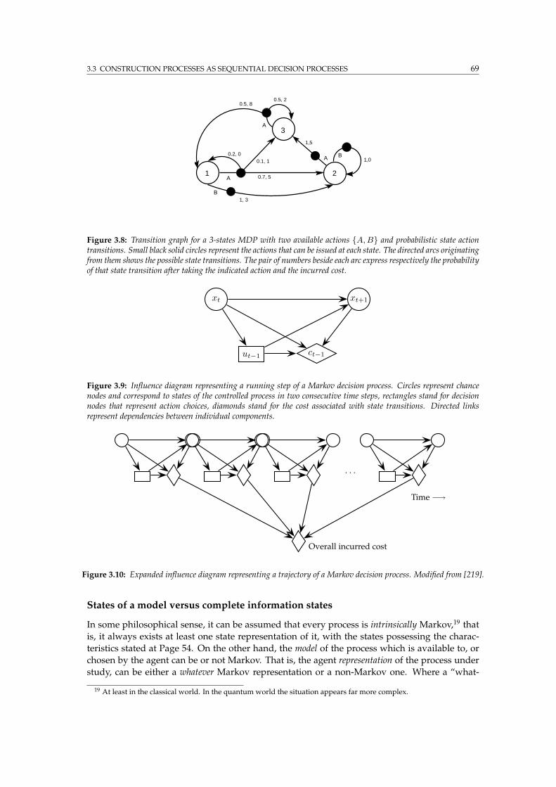
3.3 CONSTRUCTION PROCESSES AS SEQUENTIAL DECISION PROCESSES 69
A
1, 3B
0.1, 1
A
0.5, 2
A
1,5
1,0
0.5, 8
0.7, 5
0.2, 0 B
1 2
3
Figure 3.8: Transition graph for a 3-states MDP with two available actions A, B and probabilistic state actiontransitions. Small black solid circles represent the actions that can be issued at each state. The directed arcs originatingfrom them shows the possible state transitions. The pair of numbers beside each arc express respectively the probabilityof that state transition after taking the indicated action and the incurred cost.
xt xt+1
ut−1 ct−1
Figure 3.9: Influence diagram representing a running step of a Markov decision process. Circles represent chancenodes and correspond to states of the controlled process in two consecutive time steps, rectangles stand for decisionnodes that represent action choices, diamonds stand for the cost associated with state transitions. Directed linksrepresent dependencies between individual components.
· · ·
Time −→
Overall incurred cost
Figure 3.10: Expanded influence diagram representing a trajectory of a Markov decision process. Modified from [219].
States of a model versus complete information states
In some philosophical sense, it can be assumed that every process is intrinsically Markov,19 that
is, it always exists at least one state representation of it, with the states possessing the charac-
teristics stated at Page 54. On the other hand, the model of the process which is available to, or
chosen by the agent can be or not Markov. That is, the agent representation of the process under
study, can be either a whatever Markov representation or a non-Markov one. Where a “what-
19 At least in the classical world. In the quantum world the situation appears far more complex.
70 3. COMBINATORIAL OPTIMIZATION, CONSTRUCTIONMETHODS, AND DECISION PROCESSES
ever Markov representation” means a model whose mathematical properties are such that the
Markov property holds but its relationship with what can be termed the intrinsic/exact under-
lying state representation can be arbitrary. At the two extremes, the agent model can bring the
same information as the exact model or can bear no meaningful relationships with it.
To understand these facts, let us consider a physical process that, for what concerns the pre-
diction of its behavior, is perfectly described in terms of a state space X and a set of differential
equations F(X) defining the time evolution of the state variables in X . This is an “intrinsic”
representation of the system. Let us consider now a prediction agent which adopts a model of
the system based on a different set of variables, Z, which are for example defined on a small
subset Z ⊂ X of X . In this case, the prediction agent using Z will not be able, in general, to
provide fully satisfactory predictions of the system’s behavior, because the adopted description
is not anymore a proper state description. The information carried by the states of the agent
model is expected to be incompletewith respect to that carried by the exact state setX . Therefore,
it is reasonable to expect that in this case the quality of the predictions will not be so good as in
the case of using the set X . However, it is correct to say that the elements in Z are the “states”
of the adopted representation model, as long as these elements precisely play the mathematical
role of states for what concerns the model. That is, as long as a state equation in the form of
Equation C.1 can be defined. A posteriori, it will be the goodness of the predictions that the Z-
based model will be able to produce that will in some sense decide if the choice of the set Z was
or not a proper choice to represent the system under study. Likely, it will turn out that the agent
model is just an “unsatisfactory” Markov model for the system under study.
This is to stress that the intrinsic characteristics of a system, whose understanding are the
ultimate object of scientific investigation, must be seen as separated from the specific character-
istics of the model adopted by an agent to predict or control the behavior of the same system.
The Markovianity or not of a model is just a mathematical property which is assigned to the
model at design time. If the characteristics of the chosen model really match those of the sys-
tem at hand, this is another story. The level of the matching can be only assessed on the basis
of the chosen evaluation metrics. For instance, a Markov model able to provide 70% of correct
predictions can be accepted as a good model and used in practice even if it is clear that that 30%
of incorrect predictions reveal that some of the model’s states are not in correspondence with
the “true” system’s states. The search for representation models corresponding to maximally (or
fully) predictive state models for the system under study can be seen as the ultimate target of
science, resulting in a possibly never ending process of definition and refinement of agent mod-
els (e.g., see [232, 99] for insightful discussions on this subject). Generally speaking, finding the
correct state model of a system means that the model “explains” and perfectly predicts and/or
control the system’s behavior. Clearly, in the majority of the cases such an achievement simply
cannot be reached. This can be easily understood on the basis of the fact that real-world systems
involve the use of real-valued variables that cannot be practically measured and stored with the
required arbitrary precision (while in the quantum world the Heisenberg’s principle put even
more tight limits to knowledge). However, reasonable compromises can and have to be found
in practice by defining convenient evaluation metrics to score the overall quality of a model.
REMARK 3.12 (Complete information states are known for the case at hand): For the case of the
class of combinatorial problems considered in this thesis, a fully predictive state description (hereafter also
3.3 CONSTRUCTION PROCESSES AS SEQUENTIAL DECISION PROCESSES 71
called complete information states) is assumed to be known.20 In fact, the state description X comes
directly from the problem’s definition 〈C,Ω, J〉 which is available to the agent.
In a sense, the case considered here is a fortunate one. In fact, for instance, once a Markov
representation model based on states other than the complete information states described so
far is adopted, we exactly know where and in which sense there might be a loss of necessary
information. We can already predict a sort of sub-optimal performance. In other contexts the
situation is much different, since the complete information state variables and their dynamics
might not be known in advance, and there might be no cue to understand what and if something
is missing in the adopted agent model. While here the target might be the definition of a more
manageable representationmodel starting from the knowledge of the complete information state
model, in other situations the target might be the discovery of an appropriate state set which
could satisfactorily approximate the complete information one, and this discovery that has to be
done in the ignorance of the precise characteristics of the complete information states.
In order to account for the specific characteristics of the class of problems at hand, in the
following the term statewill always refer to the complete information states Therefore, in a sense,
it must be clear that we are talking not of the states of a whatever state-based representation
model but of states carrying all the useful and necessary information.
EXAMPLE 3.8: MDPS ON THE COMPONENT SET C
In some literature related to ACO, a structure equivalent to the fully connected construction graph has
been used to represent the walk of an ant in terms of an MDP whose states coincide with the nodes of
the graph (i.e., they are solution components), and state transitions coincides with the next component to
include:
MDPGC= 〈C,C, T,J 〉,
where each node ci ∈ C has |C| − 1 possible actions/transitions corresponding to transitions to all the
other nodes but itself, T says that transitions are deterministic, that is, the probability T (cj |ci, uj) = 1 if
uj = cj , 0 otherwise, and J assigns a real-valued cost to each transition.
It is easy to understand that, while such anMDP is formally correct, it is at the same time quite useless for
computing, learning or evaluating an action policy π in terms of actions u to select at each state. In fact,
representing the steps of a construction process as a walk through the nodes starting from c0, at each node
all the transitions are possible and there is no information regarding the actual feasibility of the single
choices. Actually this fact implies that there are no terminal states. That is, nodes, that once reached are
not left anymore for either the presence of a repeatedly selected self-transition, or the absence of out edges.
Terminal nodes would represent the completion of a solution. Without terminal nodes the walk on the
graph would last indefinitely while accumulating costs. In this way the walk cannot be representative
of the process of building a feasible solution of finite length. Therefore, on such a state and transition
sets, without any additional technical assumption, is in general impossible to build a feasible solution.
Accordingly, the related MDP cannot be really solved in order to discover in any efficient way the optimal
action policy π∗.
On the other hand, admitting a non-stationary MDPGC, that is, one in which the transition probabil-
ities change at each step according to an external process, the construction graph can fully represent
the construction process. In fact, if at each step t the transitions probabilities are modified such that
Tt(cj |ci, uj) = 1 if uj = cj ∧ uj 6∈ Ht, 0 otherwise, where Ht represents the set of the nodes visited so
20 The knowledge of the state description can be safely assumed for the case of static combinatorial problems. For thecase of dynamic and distributed problems (e.g., network routing), this assumption does not hold anymore, since sucha knowledge would require the knowledge of both the dynamics of the input traffic processes and the current status ofthe packet queues over the network. However, as it is explained in the following, the assumption still holds for whatconcerns the feasibility of the choices. It will be always possible to guarantee the feasibility of the routing decisions oncea decision is considered feasible if it does not give rise to a permanent cycle.
72 3. COMBINATORIAL OPTIMIZATION, CONSTRUCTIONMETHODS, AND DECISION PROCESSES
far, then the non-stationary MDPGCfaithfully represents the construction process and can in principle be
used to compute the value of the optimal policy. However, it is clear that this is a trick, since the external
process is supposed to know the complete state of the process. Unfortunately, non-stationary MDPs are
not easy at all to solve, therefore, this solution would incur computational problems similar to those faced
when trying to solve an MDP defined on the state graph.
EXAMPLE 3.9: MDPS ON THE SOLUTION SET S : LOCAL SEARCH
So far the focus has been on construction processes. Accordingly, the states have been intended in the
sense of the state of a process constructing a complete solution. As it is discussed in Appendix B this is
not by far the only and even the most popular strategy used in optimization algorithms. On the contrary,
it is common practice to search directly the set of the complete solutions.
Let us consider for instance a pure local search algorithm [344]: the search proceeds step-by-step from a
complete solution si ∈ S to another solution sj ∈ S situated in the neighborhood of the current one,
sj ∈ N (si). The search stops when a local minimum slopt ∈ Slopt ⊆ S is reached, with Slopt = s ∈S | ∀si ∈ N (s), J(si) ≥ s. Such a sequential decision process on the solution set can be represented in
the terms of an MDP:
MDPLS = 〈S,|C|∏
×C, TN ,JLS〉,
where∏|C|×C indicates the Cartesian product of order |C| of C, TN depends on the characteristics of
the neighborhoodN , and is such that if s ∈ Slopt no outer edges depart from slopt, while the incurred cost
JLS(sj |si, a), a ∈∏|C|×C, is equal to 0 for each transition which does not bring to a local minimum,
and it is equal to J(sj), ∀sj ∈ Slopt.Most of the convergence proofs or the same design of several stochastic algorithms which search directly
the solution set have been done after modeling the algorithm steps in the terms of an MDP which looks
very alike this one, possibly without the direct association between local optima and terminal states (e.g.,
see [376, 1, 55, 300] for some among the most interesting works done according to this perspective).
The recent work of Chang et al. [76] considers the application of ACO to the solution of generic MDPs,
without any specific reference to what the MDP states precisely mean. Therefore, states could coincide
with the solution set, as in the case of MDPLS . In this perspective it could be interesting to study the
possibility of letting ACO learning the state transition policy for an approximate procedure of local search,
that is, a local search which does not explore the neighborhood exhaustively. The outcome of ACO could
used to define an optimized subsampling strategy for the neighborhood. This would be a combination of
ACO and local search rather different than the usual ones, in which ACO is in a sense used to provide
effective starting points for local search. Another application of learning notions to the optimization of the
starting points of local search using MDP notions is the work of Boyan and Moore (2000) [55] (see also
Section 5.3).
3.3.5 Generic non-Markov processes and the notion of phantasma
It is a fortunate situation when it is possible to have at hand a satisfactory Markov model of a
process. In fact, in this case several appealing properties are satisfied and a plethora of methods
exist to solve the problem in an effective way. On the other hand, it often happens that the avail-
able information cannot amount to that of a state or of a sufficient statistics of it. it. Therefore,
a proper MDP cannot be designed. The class of POMDP (see Appendix C) models extend the
validity of the properties of MDPs to the case in which not a state, but an observation model for
the underlying states is available and can be used to reconstruct the true state through the step-
3.3 CONSTRUCTION PROCESSES AS SEQUENTIAL DECISION PROCESSES 73
by-step observations. In the more general case, such an observation model is either not available
to the agent with the necessary precision, or is not stationary, ending up in a generic non-Markov
representation of the system, independently from the fact that the underlying process is or is
not a Markov one. The fingerprint of a non-Markov situation is that, for necessity or choice, the
underlying complete information states are not anymore accessible to the agent. In general, this
fact dramatically affects the characteristics of the control task, and, accordingly, of the possible
control strategies.
In the case of NP-hard problems the state description explodes exponentially with the prob-
lem dimension. This fact implies that it is very unlikely that, in general, a whole state trajectory
has exploitable superpositions with previously generated ones (clearly, it depends on the pol-
icy used to generate the solution, and the more the policy is stochastic, the less there will be
exploitable superpositions):
REMARK 3.13 (Learning state trajectories is practically infeasible): Therefore, in the perspective of
solving the optimization problem using a memory-based approach as it is the case for ACO, it is practically
infeasible to gather and use memory about solutions in terms of state trajectories.
For this, the focus must shift from states to some compact representation of them. That is,
apart from the use of a state model for what concerns feasibility, an optimization agent is in some
sense forced to make use of a non-Markov representation model.
To reflect the centrality of the the agent’s point of view in the need for a “compact” represen-
tation of the problem to act upon, Birattari, Di Caro, and Dorigo [33] have introduced the term
phantasma, which is a generalization of the concept of state for the generic case of non-Markov
representations:
DEFINITION 3.21 (Phantasma): A phantasma, adopting the Greek term used by Aristotle with the
meaning of mental image,21 plays the role of the agent’s phenomenal perception of the underlying
system, that is, all what is known and retained about the system at time t for optimization purposes. The
phantasma is the result of how the agent see the system to control under the lens of the chosen/available
representation.
In the definition, the expression “for optimization purposes” has been put with the explicit
purpose to stress the fact that, in general, since the phantasma does not bring the same informa-
tion as the state, it corresponds to a non-Markov representation and therefore it cannot be used
to construct feasible solutions. However, it can be used for the purpose of optimization.
REMARK 3.14 (Phantasma as subset of state features): The use of phantasmata can be seen as equiv-
alent to the projection of the state set on a much smaller feature set, and then using the features to either
compute or learn decisions. The introduction of features implicitly involves state aggregation, and can
be conveniently seen as a contraction in the terms of the state graph. When the selected features do not
represent sufficient statistics, that is, if they do not summarize all the essential content of the states for
the purpose of control (e.g., see [23, 27]), the resulting policies are expected to be suboptimal. More in
general, a feature set is an effective one when it can capture the dominant aspects in the states.22
21 Aristotle (384–322 BC) De Anima: “The soul never thinks without a mental image (phantasma).” The same term wasreintroduced in Medieval epistemology by Thomas Aquinas (1225–1274) in the Summa Theologiae. The term phantasmata(instead of phantasms) will be used in the following to indicate the plural of phantasma.
22 In control theory, the process that carries the state into what has been call here a phantasma, is related to the conceptof state-space reduction and terms like imperfect or incomplete state are used. Here a new term is introduced to stress thefacts that: (i) the phantasma can be in principle radically different from the state, while the terms “incomplete” and“imperfect” reminds more of an entity which is either a sub-part or a noisy version of the complete information state,(ii) we are addressing in special mode the case in which the complete information state is perfectly known but it isexplicitly projected into a lower dimensional feature space for the purpose of memory and decision, such that the agentis purposely reasoning on a well defined phantasma of a state.
74 3. COMBINATORIAL OPTIMIZATION, CONSTRUCTIONMETHODS, AND DECISION PROCESSES
The parallel with the definitions in Subsection 3.3.3 is evident. In fact, as in the case of the
construction graph, the definition of a phantasma set results in a compact representation of the
state set which can be described in terms of an appropriate transformation function. Therefore,
most of the reasonings of Subsection 3.3.3 can be duplicated and generalized here.
DEFINITION 3.22 (Generating function of the phantasma representation): Given a state set X , a
phantasma set Zr is be obtained through the application of a mapping r : X → Zr (that has been called
in [33, 34] the generating function of the representation), that maps the set X of the states onto the
set Zr. The function r associates to every elements of X an element in Zr such that every phantasma
zt ∈ Zr has at least one preimage in X , but generally the preimage is not unique.
The notation r−1(zt) = xτ |r(xτ ) = zt indicates the set of states xτ whose image under r
is zt. The function r induces an equivalence relation on X : two states xi and xj are equivalent
according to the representation defined by r, if and only if r(xi) = r(xj). In this sense, a rep-
resentation can be seen as a partition of the set X . From the phantasma set Zr it is possible to
define, in parallel with the state graph, the phantasma representation graph:
DEFINITION 3.23 (Phantasma representation graph): The phantasma representation graph (or,
shortly, either the phantasma graph or the representation graph), is the graph Gr(Zr, Ur), whose edgeset Ur ⊂ Zr × Zr is the set of edges 〈zi, zj〉 for which an edge 〈xi, xj〉 ∈ C exists on the state graph and
xi and xj are the preimages under r of zi and zj , respectively. Formally:
Ur =
〈zi, zj〉∣
∣ ∃〈xi, xj〉 ∈ C : zi = r(xi), zj = r(xj)
. (3.33)
When the system is described through a generic representation r, the subset Ur(t) ⊂ Ur of
the admissible control actions at time t cannot be usually described in terms of the phantasma ztalone, but needs for its definition the knowledge of the underlying state xt. In this sense, because
of the loss of topological information, the graph Gr cannot be in general used to construct feasible
solutions. Moreover, the parallel of the weight functionC of G for the graph Gr cannot be definedin a straightforward manner for a generic r, analogously at what happened in the case of the
construction graph. In fact:
REMARK 3.15 (Construction graph as a phantasma graph): The construction graph is obtained as
the result of specific choice r ≡ , with the same as in Equation 3.20, that is, (xt) = ct.
EXAMPLE 3.10: A PARAMETRIC CLASS OF GENERATING FUNCTIONS
Let us consider a generic construction process. According to the fact that the state is made of components
added one-at-a-time, a sort of “natural” class of representation generating functions is that mapping a
state xt onto a phantasma zt defined by the sequence of the last n components added during the construc-
tion process. That is, in the particular case of states as sequences, if xt = (c0, c1, c2, . . . , ct−n, ct−n+1, . . . , ct)
is the state after t decision steps, the function rn maps xt onto the phantasma zt = (ct−n, ct−n+1, . . . , ct).
For n = t the phantasma reduces to the state, while for the other extreme case of n = 1 everything but
the last step of the construction process is forgotten. In this latter case, the obtained graph coincides with
the construction graph. This situation is also indicated with the term memoryless in related literature
on generic decision processes (e.g., [278, 353]), to stress the fact that only the last “observation” of the
process is retained and used as state feature.
As it has been anticipated and as it will be discussed in depth later, ACO ant-like agents
make use of a construction graph to represent their status for what concerns quality optimiza-
tion and framing and use memory. Equivalently, it can be said that ACO’s ants make use of a
problem representation in terms of phantasmata. That is, they purposely compact the informa-
3.4 STRATEGIES FOR SOLVING OPTIMIZATION PROBLEMS 75
tion retained about visited states. This determines some sort of aliasing of distinct states which
induces a very specific criterion for generalizing previous experience. In particular, the represen-
tation/construction graph is used to encode the values of the pheromone variables, which, in turn,
are the main parameters of the ant decision policy.
3.4 Strategies for solving optimization problems
This final part of the chapter is entirely devoted to a discussion on general-purpose approaches
to optimization, loosely classified according to the characteristics of the results they can gen-
erate and the class of problems that they address. The discussion is necessarily incomplete.
The purpose is not to provide an extensive overview of optimization problems and methods,
which would require an entire thick chapter for the most superficial of the overviews. But rather
to point out some basic and abstract notions which are in some general sense related to ACO
and which in the following will help to get a better understanding of “where” ACO is posi-
tioned within the wide universe of optimization strategies. In this sense, the following pages
can be properly seen also as a high-level description of ACO’s related work in terms of parallel
approaches. This section is complemented by the contents of Appendix B, which discusses the
important class of optimization strategies indicated here with the term “modification methods”.
After a brief discussion in-the-large on optimization strategies, which is provided in the next
Subsection 3.4.1, in the following pages the focus is shifted on general-purpose strategies for
decision optimization and learning. The starting point of the discussion will be dynamic pro-
gramming [20, 23], which represents, both from a conceptual and historic point of view, a fun-
damental bridge between optimization and control. Dynamic programming allows to discuss
the central issue of the use of state information to solve optimization problems. The importance
of dynamic programming lies also in the fact that it is at the same time a quite general-purpose
and exact approach. Very few other optimization frameworks share the same properties (e.g.,
branch-and-bound and some of its derivations, and matroids). However, dynamic program-
ming is also straight to implement, it does not require to search for bounds or any other complex
additional “device” or particularly exotic formulation. The core of dynamic programming is the
comprehensive use of information about the states and their transition structure. Information
that dynamic programming exploits possibly at the best by computing in an effective way the
value of each state and using these values to compute the optimal decision policy. However,
the famous Bellman’s curse of dimensionality [20] is still there, and for large instances this power-
ful and general state-based approach is not anymore computationally feasible. Clearly, “large”
is a relative notion, which directly depends on the available computing power. For example,
nowadays “large” for TSP instances means definitely bigger than 104 nodes, while thirty years
ago the “large” threshold already started at much below than 103 nodes. However, no matter
what large precisely means in numerical terms, the “curse of dimensionality” opens the doors
to the application of approximate methods and heuristics, either relying or not on some state in-
formation and state-values computations. The number of implementations of algorithms falling
in these broad categories is huge. Actually, just considering the vast literature in the domain
of operations research, it is apparent that a plethora of different optimization schemes and im-
plementations have appeared so far. Some of them are very effective and also quite general,
potentially embracing several different classes of problems (e.g., simplex, lagrangean relaxation,
and branch-and-cut methods [384]). However, these algorithms are not brought into the discus-
sion here since the focus is on classes of algorithms which are seen as directly related to ACO,
and, in particular, to the possible different uses of state and memory information in order to get
good or optimal solutions.
In this perspective, Subsection 3.4.2 discusses the impact of using state information and com-
76 3. COMBINATORIAL OPTIMIZATION, CONSTRUCTIONMETHODS, AND DECISION PROCESSES
puting state values, Subsection 3.4.3 briefly discusses approximate methods for computing state
values, and Subsection 3.4.4 describes policy search strategies, seen as a general class of optimiza-
tion/decision strategies which, in opposition to dynamic programming, bypass the assignment
of values to states. ACO is actually seen in this thesis mostly as an instance of a policy search al-
gorithm.23 Therefore, the main characteristics of the policy search framework will be discussed
with some detail, pointing out the different possibilities in terms of design choices, in order to
better understand later the meaning of the ACO-specific ones.
3.4.1 General characteristics of optimization strategies
Given a generic optimization problem in the form arg mins∈S J(s), the ultimate objective of any
optimization strategy is to find the element(s) s∗ ∈ S at which the global minimum of the crite-
rion J is attained. A global optimization problem, either a combinatorial or a continuous one, is
hard to solve to optimality in the general case.24 For finite combinatorial problems, the simplest
solution strategy guaranteed to find the optimal solution consists in the exhaustive enumeration
of all the possible solutions in the set S. Clearly, this approach becomes computationally infea-
sible for large problems. Once this “blind” enumeration is ruled out, the alternative becomes
the search for regularities in (S, J) that can be exploited in order to effectively reduce the search
space. That is, in order to either (i) focus the search on only those regions where the optima
(or the best solutions) are expected to be found according to analytical or heuristic criteria, or (ii)
enumerating only those solutions that can be still optimal according to a criterion that step-by-
step automatically rules out all those solutions that certainly are not optimal. In some sense, the
alternative to blind enumeration is some form of biased or informed search. Different strategies
differ for the way of defining and/or using such a bias.
The issue is if and under which conditions informed search can still guarantee to find the
optimal solution. In general, different algorithms, can provide not only solutions of different
quality, but also different levels of formal guarantees concerning the quality of the generated
solutions with respect to the searched optimal one. Usually, the amount of available resources in
terms of time and space puts strong limitations on both expected quality and formal guarantees.
Those algorithms which are guaranteed to generate the optimal solution in non-asymptotic
time (or space) are called exact algorithms. If asymptotic time is made available, exhaustive enu-
meration can always provide the optimal solutionwith the likely simplest algorithm and in finite
time. An algorithm which can guarantee the optimal solution only asymptotically is expected to
show a rate of convergence toward the optimal solution at least better than that of random search,
which is the stochastic counterpart of the exhaustive search, and which can be seen as the sim-
plest algorithm that can guarantee the optimal solution in asymptotic time. In random search
the evaluated solutions are sequentially withdrawn according to a uniform probability distribu-
tion defined over S. In a sense, sampling according to a uniform probability distribution reflects
amaximum-entropy situation: nothing is known about S, therefore the only theoretically justified
strategy consists in uniformly sampling from it. On the other side, any “informed” algorithm
will use or collect knowledge about S, such that it makes use of this knowledge to adapt the
characteristics of the sampling distribution. However, if the algorithm’s parameters are not set
in a proper way, it can easily happen that the rate of convergence to the optimal solution re-
sults worse than that of pure random search (e.g., see [375] for the case of “badly” designed
simulated annealing algorithms). In this sense, an important conceptual difference exists be-
tween continuous and combinatorial optimization. While exhaustive enumeration is impossible
23 This is however only one specific way of interpreting ACO. Other different readings can be, and are, currentlyadopted. Each different reading can serve to emphasize different aspects. This allows to import methods and resultsfrom several different fields.
24 The focus here is on problems that by necessity or by choice must be solved in algorithmic, not analytical, way.
3.4 STRATEGIES FOR SOLVING OPTIMIZATION PROBLEMS 77
in the continuous case, it is in principle always a possible alternative in the combinatorial one.
Therefore, while an approach asymptotically able to generate the optimal solution is in some
sense reasonable on the continuous, on the other side it might be of questionable utility in the
combinatorial case if its rate of convergence is worse than that of blind enumerations.
For large instances of NP-hard problems, the class of problems in which we are interested
in here, it is in general infeasible to always run exact algorithms efficiently since they will all
have worst-case exponential complexity. To cope with this intractability, a number of different
strategies have been devised in order to get solutions which are good in some well-defined
sense. Approximation algorithms produce not optimal solutions, but solutions that are guaranteed
to be a fixed percentage away from the actual optimum. Exponential algorithms have worst-case
exponential complexity, but are often successfully applied to solve to optimality instances of
reasonable size. This is the case of branch-and-bound algorithms, which are a general form of
intelligent enumeration technique. Algorithms in which the stochastic component plays a major
role cannot usually give any guarantee for what concerns the finite-time case but can guarantee,
in some probabilistic sense, to asymptotically find the optimal solution once a proper setting of
the parameters is done (e.g., simulated annealing [253] genetic algorithms [202, 226], and ACO).
The algorithms inside this class can be generally seen as specific implementations of Monte
Carlo statistical methods [367, 374] (see Appendix D for a brief introduction on Monte Carlo
techniques).
EXAMPLE 3.11: BRANCH-AND-BOUND
The branch-and-bound methods [384, Chapter 14], together with dynamic programming [20] are
among the most notable forms of intelligent enumeration techniques. In particular, branch-and-bound
algorithms are based on the idea of partitioning the solution set and of using lower bounds to construct a
proof of optimality without exhaustive search. That is, a search tree is built, where each node represents
a partition of the set of solutions and each child of a node is a subset of that partition (this is the “branch”
part). An algorithm is available for calculating a lower bound on the cost of any solution in a given subset
(the “bound” part). The search tree is searched by using the lower bounds to remove whole subtrees,
effectively reducing the number of checked solutions. Clearly, both the partitioning and the way the
lower bound is defined have a major impact on the performance of the algorithm. Under some reasonable
assumptions a branch-and-bound algorithm is guaranteed to find the optimal solution. Moreover, it enjoys
the property that if the algorithm is stopped at any time and the solution s is output, this means that the
solution s is within a ratio (s − sL)/sL from the optimal one [344, Page 444], with sL being the lowest
lower bound of any still alive node in the search tree. Unfortunately, the computational load required to
obtain good solutions is often quite heavy, and it is not always easy to find effective lower bounds.
In general, since it cannot be guaranteed to find the optimal solution in non-exponential
time/resources for each possible instance in the case of NP-hard problems, an algorithm is ex-
pected to at least generate the optimal solution once exponential or asymptotic time is allocated.
In a sense, this is a minimal requirement, that guarantee that the algorithm does not get stuck
forever in sub-optimal areas. However, the ability to asymptotically reach the optimal solution
usually does not provide any hint concerning the performance achievable in the more practical
cases when non-exponential and limited time and space resources are made available.
REMARK 3.16 (Good algorithms in practice): Informally speaking, a good algorithm can be defined
as one which can: (i) asymptotically or exponentially guarantee either the optimal solution or a precise,
possibly very small, distance from it, and (ii) in finite and non-exponential time/space show satisfactory
empirical evidence that it can find solutions of good quality inmost of the practical instances of interest.
78 3. COMBINATORIAL OPTIMIZATION, CONSTRUCTIONMETHODS, AND DECISION PROCESSES
This is the case of several popular algorithms like simulated annealing, genetic algorithms
and the same ACO, which are all (meta)heuristics:
DEFINITION 3.24 (Heuristics): An algorithm which does not provide any kind of formal guarantee on
the quality of the output that it will generate is called a heuristic.
In general, a heuristic focuses the search on regions where good solutions are expected to
be found according to heuristic criteria. In this sense, a variety of different strategies have been
adopted, each using a different bias to optimize the ratio between the expected quality of the
solutions and the use of computational resources. Local search [344], simulated annealing [253],
genetic algorithms [226], population based incremental learning [11] and tabu search [199, 200]
are all notable examples of heuristic methods which have proven to be very effective in finding
good solutions given limited resources.25
Topological issues
Since the main purpose of using a heuristic is to obtain good performance in a short running
time, there is usually some level of arbitrariness in the design choices of the algorithm. The
likely principal source of arbitrariness when designing a heuristic for a combinatorial problem
stems from the intrinsic arbitrariness related to the basic notion of neighborhood of a solution
point, and accordingly, to the arbitrariness in the definition of the topological characteristics of
the problem at hand. In fact, while in continuous spaces the notion of neighborhood of a solution
point is defined in some natural way (e.g., in Euclidean way), this is not the case for combinato-
rial problems. According to which criterion two solutions should be considered close or related
in some topological sense is a pure matter of choice in a typical combinatorial situation. It is
in general not possible to attribute to the solution set defining a combinatorial instance struc-
tural properties which are independent from the arbitrarily chosen topology. Or, in other words,
which are independent from the characteristics of the algorithm which is used to search the
set (see also the discussion on modification methods in Appendix B). On the other hand, in a
problem of continuous optimization, the natural Euclidean notion of neighborhood allows the use
(when possible in practice) of the derivatives to find the directions taking to a local optimum.
And each local optimum is know to be a local optimum with respect to the problem landscape,
while in the combinatorial case a local optimum is an optimumwith respect to the specific topol-
ogy which has been chosen to deal with the problem instance. Under a different topology the
same local optimum likely will not be a local optimum anymore, if it was not the global one.
This brief and informal discussion served to point out the potential problems related to the
definition of a strategy of biased/informed search which would result at the same time effective
in practice and theoretically justified.
25 Actually, all these algorithms are classes of algorithms, where the algorithms in the same class share some funda-mental properties and can be practically implemented according to a variety of different heuristic components. In thissense, they are all metaheuristics (see Definition 1.1). For most of these metaheuristic, a proof of asymptotic convergenceto the optimal solution has been found for some specific instances in the class. In this sense, since a guarantee on theperformance can be guaranteed, even if asymptotically, it is questionable if they should be still looked as heuristics ornot. However, since such a guarantee is usually available only for very specific instances in the class, it is reasonable tokeep referring to them as heuristics.
3.4 STRATEGIES FOR SOLVING OPTIMIZATION PROBLEMS 79
EXAMPLE 3.12: CONVEX PROBLEMS AND LINEAR PROGRAMMING
The advantage of a naturally defined metric, as it is the case for continuous search spaces, can be really
appreciated when thinking of the important class of convex problems. The problems in this class are in
some very general sense the easiest to solve to optimality because it is possible to fully exploit the character-
istics of continuous problem landscapes and the finiteness of combinatorial landscapes. For these problems
both the criterion J and the set of definition of the optimization variables are convex. These facts imply
that a local optimum is also a global one. On the contrary, in the general case, the relationship between
either a local optimum or a generic solution s ∈ S, and the searched s∗ is hard to establish. When both
J and the constraints Ω on the solution sets are linear, convex problems become linear programming
problems, which represent an important bridge between continuous and combinatorial problems. In fact,
even if the definition set for the variables is IRn the characteristics of convexity reduce the problem to the
selection of a solution among a finite convex set of possible solutions, making de facto the problem a com-
binatorial one. Khachiyan [251] firstly showed that it exists a polynomial time algorithm to solve linear
problems, by defining the so-called ellipsoid algorithm, which is, however, not really useful in practice
because of its complexity and numerical instabilities. However, both the widely known simplex algo-
rithm [101] (which is not polynomial) and all the innumerable successive variants of it, and the interior
point methods (which have weakly polynomial complexity) initiated by the work of Karmarkar [242],
are all effective ways of solving linear problems up to hundred of thousands of variables and constraints.
The use of states
If the notion of neighborhood is always somewhat arbitrary, on the other hand, the notion of
state is an intrinsic general characteristic of the problem, and the topology on the state set is well
defined. This is why the notion of state plays a special role and the state structure can be used to
define general-purpose exact optimization strategies like, in particular, dynamic programming [20,
23].
Dynamic programming is based on the decomposition of an optimization problem into a se-
quential decision problem of the form previously discussed. Each decision taken at the different
stages of a decision process results in some immediate cost but also affects the costs incurred in
future decisions, such that, in general, the quality of the resulting solution conditionally depends
on all the issued decisions. The optimization challenge consists in finding the best tradeoff be-
tween immediate and future costs. That is, when at state xi, the decision ui should be issued
taking into account both the immediate cost J (xj |xi, ui) and the desirability of the resulting next
state xj in the perspective of reaching a terminal state xs ∈ S. Dynamic programming, how it
is explained in the next section, provides a mathematical formalization of this tradeoff by intro-
ducing an efficient way to assign the correct value of desirability to states. The core idea in dynamic
programming consists in the use of value functions to organize and structure the search for good
decision policies.
DEFINITION 3.25 (Value function): A value function is a function V : X → IR which assigns a
real value to each state in the terms of either the cost-to-go from that state to a terminal state or the
accumulated cost from the initial state, according to the current action policy π. Accordingly, the value
of each state x ∈ X is indicated by V π(x).
That is, taking the state x as a starting state, the combination of the costs incurred after each
state transition while moving from x to xs ∈ S by applying the current policy π, or vice versa
from xs to x, represents the value of state x under that policy. If transitions are probabilistic
this value can be only assigned as an expectation. According to the terminology used in the

80 3. COMBINATORIAL OPTIMIZATION, CONSTRUCTIONMETHODS, AND DECISION PROCESSES
context of dynamic programming, the value in terms of cost-to-go correspond to the use of
backward recursion, while the use of accumulated costs corresponds to the use of forward recursion.
These two equivalent models are discussed more in detail in the next subsection. The notion of
value function can be generalized by that of utility function, which assigns to a state a value
representing, in any convenient sense, the utility of being in that state.
When the cost structure is additive, the use of value functions to describe the structure of
problem states results in an efficient way to compute the optimal action policy. Since the state
structure carries all the important information about the problem, dynamic programming meth-
ods, when properly designed, can guarantee optimality in non asymptotic time (for deterministic
problems).
To emphasize the special role played by the use of states and state-values, a clear distinction
is made between the vast classes of algorithms which make use or not of these notions:
REMARK 3.17 (The value-based and policy search approaches): The approach to problem solution
which makes use of value functions is indicated with the term value-based (e.g., [27]), since it relies on
the estimation of the value of occupying a particular state of the environment or of taking a particular
action in response to being in a state.
On the other hand, policy searchmethods (e.g., [350]) are that vast class of methods searching for optima
directly in the space of the possible decision policies bypassing the direct assignment of a value to states in
the sense specified by value functions.
Value-based methods are the general methods of election when a complete model of the
problem (states and costs) is known, accessible, and in practice computationally tractable. On
the other hand, when a trusting state description is neither available nor computationally tractable,
policy search methods appears more suitable for use. Unfortunately, in the general case, the
use of either incomplete state information or not state information at all results in algorithms
which come with no guarantee of optimality (at least non in finite time). However, policy search
methods amounts several among the most popular and efficient optimization heuristics, like the
already mentioned genetic algorithms, simulated annealing, local search, tabu search, and ACO.
In a sense, the use or not of state information and value functions creates a clear distinction
among algorithms. Two major classes of general approaches can be identified on the basis of
the amount of the problem information they make use of. The following sections discuss the
characteristic of these two classes more in detail, showing, in particular, the practical problems
related to value-based approaches and supporting in a sense the design choices of ACO, which
relies on state information only for what concerns feasibility. Clearly, also policy search is by
no means free from problems, but it is expected to be more robust than value-based approaches
when phantasmata must be used instead of states due to the large cardinality of the state set.
3.4.2 Dynamic programming and the use of state-value functions
Dynamic programming consists in an efficient way to compute the optimal decision policy by
using value functions, and, in particular, by exploiting the properties of global consistency ex-
isting among the optimal state values.
Let us consider the general case of a finite horizon MDP with undiscounted total cost cri-
terion and probabilistic state transitions (see Equation C.5 in Appendix C). The value function
derives directly from the optimization criterion and takes the form:
3.4 STRATEGIES FOR SOLVING OPTIMIZATION PROBLEMS 81
V π(x) = Eπ
[
H∑
t=0
J (xt+1| xt, uπt )∣
∣
∣x0 = x
]
= Eπ
[
J (x1| x0, uπ0 ) +
H∑
t=1
J (xt+1| xt, uπt )∣
∣
∣x0 = x
]
= Eπ
[
J (x1| x0, uπ0 ) + V π(x1)
∣
∣
∣x0 = x
]
∀x ∈ X.
(3.34)
The above equations define one-step relationships between the values of pairs of states under
the same action policy. That is, the state values are not independent but tightly related to each
other. The knowledge of the value of state xj can be used in turn to compute the value of state
xj−1, once the cost of the transition from xj−1 to xj is known as well as the probability of such
transition under the current policy and state transition structure.
The joint set of the V π(x)’s values for all x ∈ X represents a direct evaluation of the policy π.
In fact, each V (x) tells which is the sum of costs which one is expected to incur from that state.
We will see in the Subsection 3.4.4 that without a value function, and, more in general, without
states, it becomes much less straightforward to evaluate a policy.
The relationship 3.34 can be even further expanded and made an n-step relationship:
V π(x) = Eπ
[
c0 + c1 + c2 + . . . cn−1 + V π(xn)∣
∣
∣x0 = x
]
∀x ∈ X (3.35)
with ci = J (xi+1| xi, uπi ).
All these equations express the global consistency existing among the state values under the
generic policy π. But more interesting is the case for the optimal policy π∗, which is the one that
is searched:
DEFINITION 3.26 (Bellman’s optimality equation [20]):
V ∗(x) = minu∈U(xt)
Eπ∗
[
J (xt+1| xt, uπ∗
t ) + V ∗(xt+1)∣
∣
∣xt = x
]
, ∀x ∈ X. (3.36)
In simple terms, the Bellman’s (one-step) optimality equation expresses the fact that the value
of a state under an optimal policy must equal the combination of the costs following after taking
the locally best action for that state and keeping acting according to the optimal policy. The
validity of the Bellman’s equation is based on the Bellman’s principle, which can be shortly and
informally stated as:
DEFINITION 3.27 (Bellman’s principle): In a state graph all the sub-paths of an optimal path must be
in turn optimal sub-paths.
The Bellman’s optimality equations define a precise relationship between state values and
optimal policy. Therefore, they can be used in turn to compute the optimal policy. The equa-
tions are actually a system of |X| nonlinear equations in |X| unknowns. If all the necessary
information on the environment are available (i.e., states, state transitions and costs dynamics),
then in principle one can solve the system with any one of a variety of available methods. Once
V ∗ has been computed, π∗ is any policy which is locally (in the sense of the states) greedy with
respect to the V ∗ values. Therefore, locally optimal choices result in a globally optimal policy:
π∗(x) = arg minu∈U(x)
[
J (xt+1| xt, u) + V ∗(xt+1)∣
∣ xt = x]
, ∀x ∈ X. (3.37)
82 3. COMBINATORIAL OPTIMIZATION, CONSTRUCTIONMETHODS, AND DECISION PROCESSES
The set of states for which the Bellman’s relationships must hold in general depends on the
initial conditions. If any x ∈ X can be a starting state, then Equation 3.37 must be solved for all
the possible states. In fact, since each state-value is related to the others according to 3.36, to be
optimal a policy must necessarily optimize the joint values of all states. When only a subset of
the states can act as starting states, then the Bellman’s equation needs to be solved only on the
related subset of the problem states. That is, in general, the following relationship must hold:
V π∗
(x) < V π(x), ∀ π ∧ x ∈ X interested by the initial conditions. (3.38)
For every finite discounted MDP an optimal policy π∗ satisfying the relationship 3.38 exists
in the set of the stationary deterministic policies [369]. In the case of different cost criteria, the
situation becomes more complex, and relationships more sophisticated than 3.38 have to be
used to derive the optimal policy. For example, the notions of gain and bias optimality are used
to weight in different way the relative contribution given by the costs associated to transient,
recurrent and adsorbing states in the Markov chain. The optimality metric called n-discount-
optimal [431], relates the discounted and the average frameworks providing a quite general way
to define optimality in anyMDPs (theMahadevan’s paper [287] contains an insightful discussion
and good references on this subject).
Among the different ways for solving the system 3.36, dynamic programming is a sort of
general template of election. In fact, under the name of dynamic programming goes a collection
of iterative techniques which explicitly exploit the Bellman’s relationships among the state value
functions.
The description of the state values relationships given in the previous equations is based on
what is called backward recursion, since the values are implicitly computed from the terminal to
the initial states. Equivalently, a forward recursion formulation can be used. The value of a state
is in this case the accumulated cost starting from the initial state. The Bellman’s equation for a
deterministic case becomes:
V ∗(xt) = minu∈U(xt−1)
J (xt| xt−1, uπ∗
t−1) + V ∗(xt−1), (3.39)
that has to be compared to the one of backward recursion:
V ∗(xt) = minu∈U(xt)
J (xt+1| xt, uπ∗
t ) + V ∗(xt+1). (3.40)
In practice, backward recursion requires the precise knowledge of terminal states, while forward
recursion does not, but needs a breadth-first search to expand each state value. In the forward
case the state value corresponds to the accumulated cost from the starting state, while in the back-
ward case the value is the cost-to-go to a terminal state. Both models can be usually applied to
the class of combinatorial problems of interest in this thesis.
In spite of the specific (backward/forward) model, dynamic programming is always based
on (i) the characterization of the optimization problem in the terms of the Bellman’s optimality
equations 3.36, and (ii) on the definition of twomain ways to solve the equation system: policy it-
eration and value iteration. The literature on dynamic programming is extensive, since it has been
widely used in the fields of control, reinforcement learning and operations research. Therefore,
it is not really necessary to explain here the details of these two techniques. It suffices to say that
both are based on the simple scheme of generalized policy iteration [414] , reported in the pseudo-
code of the Algorithm box 3.2, in which phases of policy evaluation and policy improvement are
alternated. Policy evaluation means that the equation system 3.34 is solved, exactly or approx-
imately for a specific policy π, and the values of V π are computed. In the policy improvement
phase, the policy π is changed in order to go towards the direction of optimizing the costs-to-go
of of the states according to the newly estimated values of V π . If both the phases are carried out
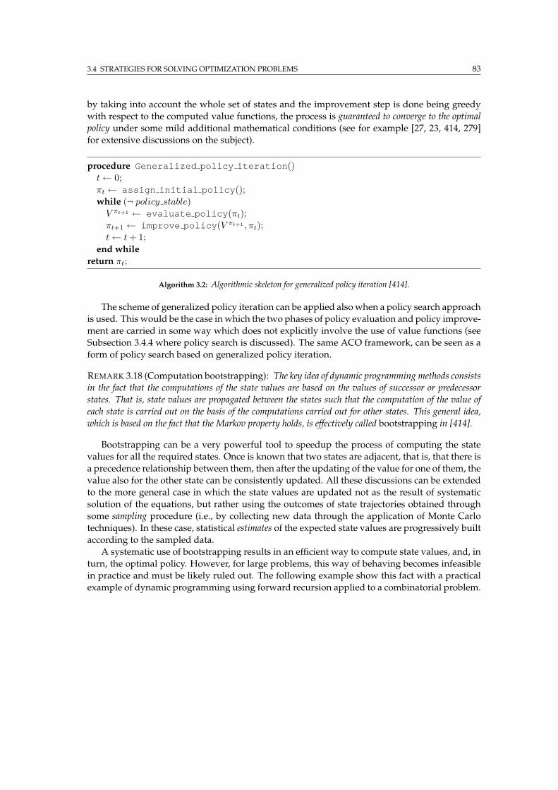
3.4 STRATEGIES FOR SOLVING OPTIMIZATION PROBLEMS 83
by taking into account the whole set of states and the improvement step is done being greedy
with respect to the computed value functions, the process is guaranteed to converge to the optimal
policy under some mild additional mathematical conditions (see for example [27, 23, 414, 279]
for extensive discussions on the subject).
procedure Generalized policy iteration()
t← 0;
πt ← assign initial policy();
while (¬ policy stable)V πt+1 ← evaluate policy(πt);
πt+1 ← improve policy(V πt+1 , πt);
t← t+ 1;
end while
return πt;
Algorithm 3.2: Algorithmic skeleton for generalized policy iteration [414].
The scheme of generalized policy iteration can be applied also when a policy search approach
is used. This would be the case in which the two phases of policy evaluation and policy improve-
ment are carried in some way which does not explicitly involve the use of value functions (see
Subsection 3.4.4 where policy search is discussed). The same ACO framework, can be seen as a
form of policy search based on generalized policy iteration.
REMARK 3.18 (Computation bootstrapping): The key idea of dynamic programming methods consists
in the fact that the computations of the state values are based on the values of successor or predecessor
states. That is, state values are propagated between the states such that the computation of the value of
each state is carried out on the basis of the computations carried out for other states. This general idea,
which is based on the fact that the Markov property holds, is effectively called bootstrapping in [414].
Bootstrapping can be a very powerful tool to speedup the process of computing the state
values for all the required states. Once is known that two states are adjacent, that is, that there is
a precedence relationship between them, then after the updating of the value for one of them, the
value also for the other state can be consistently updated. All these discussions can be extended
to the more general case in which the state values are updated not as the result of systematic
solution of the equations, but rather using the outcomes of state trajectories obtained through
some sampling procedure (i.e., by collecting new data through the application of Monte Carlo
techniques). In these case, statistical estimates of the expected state values are progressively built
according to the sampled data.
A systematic use of bootstrapping results in an efficient way to compute state values, and, in
turn, the optimal policy. However, for large problems, this way of behaving becomes infeasible
in practice and must be likely ruled out. The following example show this fact with a practical
example of dynamic programming using forward recursion applied to a combinatorial problem.
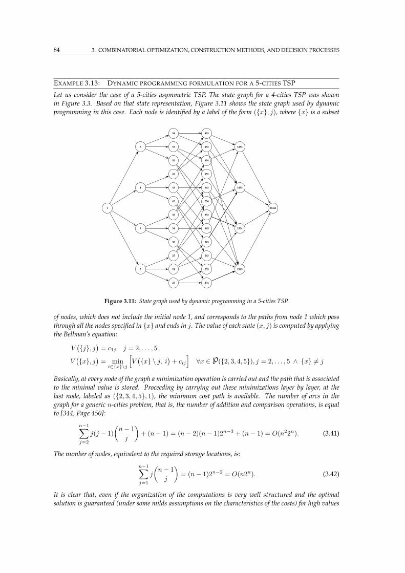
84 3. COMBINATORIAL OPTIMIZATION, CONSTRUCTIONMETHODS, AND DECISION PROCESSES
EXAMPLE 3.13: DYNAMIC PROGRAMMING FORMULATION FOR A 5-CITIES TSP
Let us consider the case of a 5-cities asymmetric TSP. The state graph for a 4-cities TSP was shown
in Figure 3.3. Based on that state representation, Figure 3.11 shows the state graph used by dynamic
programming in this case. Each node is identified by a label of the form (x, j), where x is a subset
1
2
3
4
5
23
24
25
32
34
35
42
43
45
52
53
54
234
235
243
245
2345
2534
2453
3452
23451
345
253
254
342
352
354
452
453
Figure 3.11: State graph used by dynamic programming in a 5-cities TSP.
of nodes, which does not include the initial node 1, and corresponds to the paths from node 1 which pass
through all the nodes specified in x and ends in j. The value of each state (x, j) is computed by applying
the Bellman’s equation:
V(
j, j)
= c1j j = 2, . . . , 5
V(
x, j)
= mini∈x\j
[
V(
x \ j, i)
+ cij
]
∀x ∈ ℘(2, 3, 4, 5), j = 2, . . . , 5 ∧ x 6= j
Basically, at every node of the graph a minimization operation is carried out and the path that is associated
to the minimal value is stored. Proceeding by carrying out these minimizations layer by layer, at the
last node, labeled as (2, 3, 4, 5, 1), the minimum cost path is available. The number of arcs in the
graph for a generic n-cities problem, that is, the number of addition and comparison operations, is equal
to [344, Page 450]:
n−1∑
j=2
j(j − 1)
(
n− 1
j
)
+ (n− 1) = (n− 2)(n− 1)2n−3 + (n− 1) = O(n22n). (3.41)
The number of nodes, equivalent to the required storage locations, is:
n−1∑
j=1
j
(
n− 1
j
)
= (n− 1)2n−2 = O(n2n). (3.42)
It is clear that, even if the organization of the computations is very well structured and the optimal
solution is guaranteed (under some milds assumptions on the characteristics of the costs) for high values
3.4 STRATEGIES FOR SOLVING OPTIMIZATION PROBLEMS 85
of n the approach becomes practically infeasible if implemented without any modification, while nowadays
heuristic methods can easily solve to optimality TSPs up to thousands of cities [237].
Generalizations of the basic dynamic programming approach
The application of dynamic programming requires full knowledge of the Markov model. When
this is not the case, or, more in general, when some components of the Markov model are not
explicitly available or manageable, the basic dynamic programming ideas must be properly re-
vised and adapted.
For instance, if one know does not know where the terminal states are in the search space
(e.g., this might be the typical case of learning from an unknown environment), backward re-
cursion cannot be used. Forward recursion can be still used but if the number of states is large
the stage-by-stage breadth-first operation is usually too heavy to carry out. An effective alterna-
tive in this case are the A∗ algorithms [336], which combine forward recursion with a domain-
specific function h(x) used to estimate V (x) for the states ahead. The estimation function h re-
quires little or no state “look-ahead”, yet it can still bring to an optimal solution assumed that
h(x) ≥ V (x), ∀x ∈ X . That is, when h is a heuristic function which never underestimates the
value of a state. The variant of A∗ called Real-Time A∗ [16] modifies some A∗ behaviors in order
to quickly get a possibly good, even if not optimal solution, and which can incrementally learn
from experience.
Another common situation is that when the costs are always zero except for the transitions
to terminal states (e.g., a foraging agent looking for food gets its reward only when it actually
arrives to the food site). This is the case of delayed rewards/costs, which is typical in reinforcement
learning domain. This situation cannot be tackled efficiently by dynamic programming, since it
is not possible to discriminate the value of all states far more than one transition step from the
terminal states. This case, as well as that in which the states but not the transition and cost func-
tions of the Markov model are known in advance, are domains of application of reinforcement
learning algorithms like Q-learning [442] and SARSA [414], which generalize the bootstrapping
ideas of dynamic programming. For instance, Q-learning constantly adjust the estimate of V (x)
while back-propagating later rewards to the earlier stage. Q-learning does not need the knowl-
edge of the transition function or of the cost function: after executing an action it needs only to
receive from the environment a cost signal which depends on the current environment state and
issued action. Upon receiving the action, the state of the environment changes according to a
probabilistic state transition whose knowledge is not required, since it is assumed that the new
current state can be identified by the controlling agent. However, if the environment’s model is
available, this information can be fruitfully used inside Q-learning-like schemes (e.g., [415]).
REMARK 3.19 (The Markov model is assumed fully accessible): In general, for the class of com-
binatorial problems considered here the characteristics of the Markov model can be always assumed as
accessible to the optimization agent. However, a straightforward application of dynamic programming
would result either computationally infeasible in practice for medium/large NP-hard problems, or possi-
bly flawed when the situation is not stationary (e.g., communication networks problems).
Bootstrapping and Monte Carlo techniques
One can think that it could be possible to partially alleviate the computational burden by using
some compact representations or phantasmata instead of states. Actually, the point is that the
Bellman’s equations, and the Markov property, which make bootstrapping possible, hold only
for states.
86 3. COMBINATORIAL OPTIMIZATION, CONSTRUCTIONMETHODS, AND DECISION PROCESSES
REMARK 3.20 (Bellman’s optimality equations hold only for states): The Bellman’s principle and
equations are really meaningful when applied to states. In fact, if applied to entities which do not have
behave like states (e.g., phantasmata) the expectations will be computed on the basis of wrong probability
distributions, resulting in policies which do not coincide with the optimal policies that would be obtained
by using the system’s complete information states.
To see this, let us rewrite the value function by expliciting the expectation operator:
V π(x) =∑
u∈U
Pr(u|π, x)[
∑
x′∈X
Pr(x′|x, u)[
J (x′| x, u) + V π(x′)]
]
. (3.43)
If x represents for instance the last observation, and this does not coincides with the state, then
the weighting probabilities Pr(u|π, x) and Pr(x′|x, u) are expected to be wrong. In fact, the last
observation alone is not expected to be sufficient to determine the correct probability models for
the transitions in the system. If this would be the case this would mean that the observations
enjoy theMarkov properties, that is, they would coincide with the states, but this hypotheses has
been ruled out at the beginning of the reasonings. Once the Bellman’s equations are solved using
the “wrong” transition probabilities, the resulting policy is not expected to be the optimal one, in
the sense of being optimal with respect to the underlying complete information states. More in
general, the resulting policy might have no meaningful relationships with the policy that would
have been obtained by solving the Bellman’s optimality equations using the states of the system
under study. Singh, Jaakkola, and Jordan [392] discusses several practical examples of such a
situation, showing how unrelated can result the behavior and performance of “optimal” policies
computed according respectively to states and observations. While Littman [278] investigates
more specifically the characteristics of memoryless policies.
These facts does not mean that is always inappropriate to use value-based strategies in non-
Markov situations. Actually, this has been done, and sometimes also with good success (see for
example [280, 277] for applications of value-based approaches in POMDPs using observations
instead of information states). However, in order to be such an approach successful, the state
aliasing determined by the agent representation of the underlying Markov problem has to be
minimal. That is, most the distributions of the adopted observation model must be peaked
around the true states. Moreover, it can greatly help if the agent can find alternative ways to
include some information from its past history at the time the policy is estimated and updated
(e.g., in [280] eligibility traces [414, 442, 391] are used for this purpose).
REMARK 3.21 (Bootstrapping and global propagation of incorrect estimates): It must be under-
stood that the use of Bellman’s equations means that the state structure is seen as a fully connected
network of propagating estimates. A change in one estimate propagates all over the network moving
through adjacent nodes. If this can be clearly seen as an effective way to save computations, it must be
seen also in terms of a system which is potentially extremely fragile: a single locally “wrong” estimate can
propagate throughout the whole state network determining globally wrong estimates.
Therefore, for instance, if phantasmata are used instead of states, it can easily happen that
incorrect estimates are built for some phantasma and quickly propagated, creating an overall
status of inconsistency. A similar situation can happen in the case of dynamic optimization
problems (e.g., routing in communication networks): because of the problem’s dynamics, local
state estimates can become out-of-date while they are still traveling across the network and being
used to build up other (wrong) estimates. These facts actually make value-based methods less
robust than those based on policy search. If the situation is static, the whole state structure is
known and accessible, and no errors happen, value-based methods result very effective. On the
other hand, if anyone of these conditions do not hold anymore the system can potentially show
a dramatic negative drop of performance.
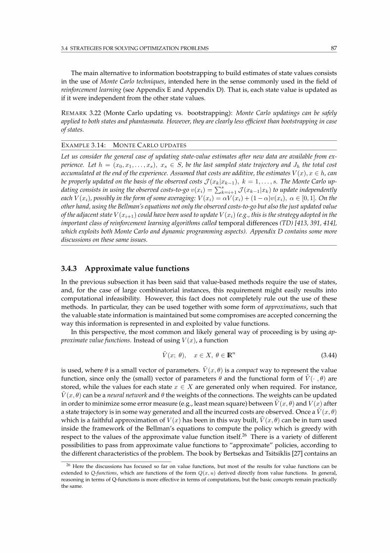
3.4 STRATEGIES FOR SOLVING OPTIMIZATION PROBLEMS 87
The main alternative to information bootstrapping to build estimates of state values consists
in the use of Monte Carlo techniques, intended here in the sense commonly used in the field of
reinforcement learning (see Appendix E and Appendix D). That is, each state value is updated as
if it were independent from the other state values.
REMARK 3.22 (Monte Carlo updating vs. bootstrapping): Monte Carlo updatings can be safely
applied to both states and phantasmata. However, they are clearly less efficient than bootstrapping in case
of states.
EXAMPLE 3.14: MONTE CARLO UPDATES
Let us consider the general case of updating state-value estimates after new data are available from ex-
perience. Let h = (x0, x1, . . . , xs), xs ∈ S, be the last sampled state trajectory and Jh the total cost
accumulated at the end of the experience. Assumed that costs are additive, the estimates V (x), x ∈ h, canbe properly updated on the basis of the observed costs J (xk|xk−1), k = 1, . . . , s. The Monte Carlo up-
dating consists in using the observed costs-to-go v(xi) =∑sk=i+1 J (xk−1|xk) to update independently
each V (xi), possibly in the form of some averaging: V (xi) = αV (xi) + (1−α)v(xi), α ∈ [0, 1]. On the
other hand, using the Bellman’s equations not only the observed costs-to-go but also the just updated value
of the adjacent state V (xi+1) could have been used to update V (xi) (e.g., this is the strategy adopted in the
important class of reinforcement learning algorithms called temporal differences (TD) [413, 391, 414],
which exploits both Monte Carlo and dynamic programming aspects). Appendix D contains some more
discussions on these same issues.
3.4.3 Approximate value functions
In the previous subsection it has been said that value-based methods require the use of states,
and, for the case of large combinatorial instances, this requirement might easily results into
computational infeasibility. However, this fact does not completely rule out the use of these
methods. In particular, they can be used together with some form of approximations, such that
the valuable state information is maintained but some compromises are accepted concerning the
way this information is represented in and exploited by value functions.
In this perspective, the most common and likely general way of proceeding is by using ap-
proximate value functions. Instead of using V (x), a function
V (x; θ), x ∈ X, θ ∈ IRn (3.44)
is used, where θ is a small vector of parameters. V (x, θ) is a compact way to represent the value
function, since only the (small) vector of parameters θ and the functional form of V (· , θ) are
stored, while the values for each state x ∈ X are generated only when required. For instance,
V (x, θ) can be a neural network and θ the weights of the connections. The weights can be updated
in order tominimize some errormeasure (e.g., least mean square) between V (x, θ) and V (x) after
a state trajectory is in someway generated and all the incurred costs are observed. Once a V (x, θ)
which is a faithful approximation of V (x) has been in this way built, V (x, θ) can be in turn used
inside the framework of the Bellman’s equations to compute the policy which is greedy with
respect to the values of the approximate value function itself.26 There is a variety of different
possibilities to pass from approximate value functions to “approximate” policies, according to
the different characteristics of the problem. The book by Bertsekas and Tsitsiklis [27] contains an
26 Here the discussions has focused so far on value functions, but most of the results for value functions can beextended to Q-functions, which are functions of the form Q(x, u) derived directly from value functions. In general,reasoning in terms of Q-functions is more effective in terms of computations, but the basic concepts remain practicallythe same.
88 3. COMBINATORIAL OPTIMIZATION, CONSTRUCTIONMETHODS, AND DECISION PROCESSES
exemplary treatment of the whole subject. A notable and effective class of algorithms based on
these notions and specifically designed for combinatorial optimization problems is that of rollout
algorithms of Bertsekas, Tsitsiklis, and Wu [28] (discussed in Section 5.3.
Without diving into unnecessary details, what is interesting to remark here is the fact that us-
ing approximate value functions reduces the problem of the computation of the (optimal) value
function to the learning of the values of a parameter vector θ. The hypotheses behind this trans-
formation is that if V is a good approximation of V ∗, then a greedy policy based on V is in turn
close to the optimal policy π∗. An important general result in this sense is that if ‖ V − V ‖= ǫ,
for some ǫ ≥ 0 and for all states, where ‖ · ‖ is a maximum norm, then if π is a greedy policy
based on V it results that [27, Page 262]:
‖ V π − V ∗ ‖ ≤ 2αǫ
1− α, (3.45)
for an α-discounted MDP.
Clearly, since an approximation is used, the learned V ∗(x, θ∗) can in principle bear no mean-
ingful relationships with the real V ∗(x). The appropriate choice of (i) the approximation archi-
tecture, (ii) the parameter vector θ, and (iii) the procedure to optimize the values of θ, (iv) the
ways of sampling the state trajectory (possibly using Monte Carlo techniques, see Appendix D),
are all of primary importance to minimize in some meaningful sense the chosen error measure
between the functions V and V ∗
3.4.4 The policy search approach
The two previous subsections have discussed both exact and approximate value-based meth-
ods. While the effectiveness of such methods has been pointed out, the computational problems
potentially related with their use might limit their practical application.
In general, when a state description of the problem at hand either cannot be used in practice
in terms of value functions or it is not fully available, optimization algorithms from the class of
policy searchmight result more effective than those from the value-based class.
Policy search has been broadly defined in Remark 3.17 as the class of all those algorithms
which bypass the assignment of values to states to compute the decision policy. The search for
an optimal policy is executed directly on the policies’ definition space, not “indirectly” through
the computation of state values. Clearly, being such class of methods defined by a “proscription”
rather than a “prescription”, is expected to embrace a really vast number of different possible
implementations.
The fact that policy search does not rely on value functions means also that it is not either
anymore necessary to use states since it is not anymore necessary to compute their values. There-
fore, it is possible to define the policy’s domain in more general terms:
REMARK 3.23 (Generalization of the policy’s domain): Generalizing the previous Definition 3.16,
in the case of policy search a policy can be seen as a mapping from history of observations and actions to
actions. Or, more generically, from agent situations, whatever this could mean, to actions. Clearly, this
does not preclude the policy for being defined on the underlying state set:
π : Z × U → U, (3.46)
with Z ⊆ X , and U ⊆ C. Assuming without loss of generality that the policy is stochastic, this means
that:
πǫ(z, u) = Pr(ut = u | zt = z), z ∈ Z, u ∈ U(z) (3.47)
The use of the letter Z wants to reflect the fact that, according to Definition 3.21, the policy is
generically defined on a phantasma set.

3.4 STRATEGIES FOR SOLVING OPTIMIZATION PROBLEMS 89
If on one side the very possibility to define the policy’s domain in terms of any convenient
set of state features gives great freedom to an algorithm designer, it is by no means free from
complications with respect to the value-based case.
In particular, once neither states nor value functions are in use anymore, it is not precisely
defined how a policy can be evaluated, and, in turn, optimized. In the value-based case, the value
of a policy is automatically expressed in terms of the state values. One clearly wants to find
the policy that optimizes the joint costs-to-go for each state. On the other hand, it has already
pointed out (Remark 3.20) that Bellman’s relationships only hold for states. Therefore, when
history of observations which do not coincide with complete information states are used, is in
general not anymore possible to optimize the value of each observation of each underlying state
(e.g., see [392]). This fact implies that in these cases a different, and in some sense more general,
definition of quality and optimality of a policy must be given, other than that expressed by
Equations 3.37 and 3.38.
Let us call ht the history of a whole cycle of interaction of length t steps between the agent
and the environment. Each ht results in a sequence of actions from the agent and associated cost
signals from the environment. The combination of the costs incurred during the whole length of
the agent’s history represents the numerical outcome J(ht|π) resulting from the application of
the agent’s current policy. This value is clearly a measure of the quality of the adopted policy. If
the policy is stochastic, and/or the starting point is assigned according to some distribution of
probability over the states, the value of the policy must be calculated in terms of an expectation.
DEFINITION 3.28 (Value of a policy when the policy domain is not the state set): Since any policy
πǫ defines a conditional distribution Pr(h|πǫ), h ∈ H , on the set H of all the possible histories of the
agent, the value V of policy πǫ is the expected overall cost computed according to this same distribution:
V(πǫ) = Eπǫ
[
J(h)]
=∑
h∈H
J(h)Pr(h|πǫ). (3.48)
This definition coincides with that based on state values once the histories are intended as infor-
mation states. While in the value-based case the value function V defined on the states can be
directly used to evaluate the policy, in the case of not using states the quality of a policy must be
in general evaluated by executing the policy itself (or by simulating its execution) to observe the
resulting costs. This fact asks for an effective sampling strategy in the set of the agent possible
histories in order to obtain unbiased and low variance estimates for the policy’s value.
It is apparent that the policy which minimizes the value of the expected value V is the policy
which minimizes also the original combinatorial problem. In practice, the optimal policy π∗
is that which assigns probability 1 to the agent history h∗ corresponding to the minimal cost
value J∗ of J . Any other policy which assigns a probability greater than one to histories h with
associated cost J(h) > J∗ is in some sense sub-optimal. However, according to the fact that the
policy can be safely assumed to be a stochastic one, it is satisfactory to find a policy πǫ which
minimizes the expected value in probabilistic sense:
Pr
‖ V πǫ − Vπ∗ ‖≥ δ
= 0, for some δ ≥ 0, (3.49)
and for some suitable norm ‖ · ‖. This relationship expresses the fact that, in the general case,
a policy search algorithm can only guarantee asymptotic convergence in probability. This fact can
be easily understood as the result of the missing state information. Search in the policy set
amounts to the search in the same solution set of the original global optimization problem. The
core difference between value-based methods and generic policy search methods consists in the
fact that the formers exploits the underlying state structure of the problem, while the latters do
not exploit any particular information concerning the intrinsic structure of it.
90 3. COMBINATORIAL OPTIMIZATION, CONSTRUCTIONMETHODS, AND DECISION PROCESSES
However, it is an empirical evidence that optimization/decision algorithms based on the pol-
icy search general scheme are usually quite effective, often able to provide performance better
than those provided by their value-based counterparts for large problems. Popular metaheuris-
tic like genetic algorithms, simulated annealing, iterated local search [358], population based in-
cremental learning [11], evolutionary strategies [172], genetic programming [260], and the same
ACO, can all be seen as specific implementations of policy search algorithms for optimization,
while the successful application of policy search in control and reinforcement learning domains
is ever increasing (a comprehensive treatment of this specific subject and a list of applications
can be found in [350]). To not to mention the excellent performance showed by policy search al-
gorithms in the case of application to telecommunication network problems, which pose severe
restrictions on the ability to know and use problem states. This specific subject will be throughly
discussed in the second part of the thesis.
Broadly speaking, the empirical evidence for good performance can be likely explained by
considering the proscription nature of policy search, which does not impose a precise way of
designing an algorithm, as in some sense dynamic programming does. This design flexibility
can easily accommodate for a wide range of possible strategies, and, in particular, for strategies
ad hoc for the problem at hand. Therefore, if dynamic programming methods naturally exploits
the general characteristics of a problem in terms of its state structure, the design of policy search
can be addressed at the exploitation of the specific characteristics (known, learned or supposed)
of the problem. How it is easy to figure out, this fact can often result in the design of rather
effective algorithms.
Design issues for policy search algorithms
At a general level, three major design components can be identified, from which the global
characteristics and performance of the resulting algorithm largely depends:
1. the functional form of the policy π,
2. what the history information zt ∈ Z retained at time t consists of,
3. how the set of possible histories is sampled to evaluate the policy in an effective way.
The functional form of the policy determines how the available information is used to assign
a value of desirability to the different choices and according to which mechanisms the selection
actually happens. Therefore, the characteristics of the policy defines also the level of exploration,
which is usually an important aspect of a policy search algorithm since it affects the sampling of
agent histories. Monte Carlo techniques for stochastic sampling are in this sense a fundamental
tool often used to design this part of the algorithm, as well as the part concerning with how to
sample histories in order to obtain unbiased and and low variance estimates for policy evalua-
tion and improvement.
Regarding the retained history information, it is clear that when a state description is avail-
able and manageable, it can be fruitfully used. For instance, zt values can coincide with the
states xt. On the contrary, in the more general case of using a non-Markov representation, differ-
ent choices forZ can easily take to dramatically different behaviors and quality. As it has already
remarked, sufficient statistics, or state features which conserve the dominant aspects in the states
should be used in order to reduce the negative impact coming from the loss of state information.
It is evident that different design choices for just these three major aspects can result in algo-
rithms with different characteristics.
3.4 STRATEGIES FOR SOLVING OPTIMIZATION PROBLEMS 91
From global optimization to learning on parametric spaces
In spite of the available freedom when designing a policy search algorithm, searching in the
space Π of all possible policies still means solving a huge and usually non-convex problem of
global optimization which is by no means easier of the original combinatorial problem. There-
fore, one more general and rather popular design strategy consists in transforming the policy
search problem at hand into a learning problem of reasonably small size:
REMARK 3.24 (From optimization to learning on a parametric class of policies): The global op-
timization problem consisting in the search for the optimal stochastic policy can be conveniently trans-
formed into a possibly easier problem by restricting the possible policies to a single parametric class of
the type:
πǫ(· ; θ), πǫ(θ), (3.50)
also shortly indicated with πǫ(θ). In this way, the policy search optimization problem is transformed into
the problem of learning the values to the parameter vector θ such that the value of V(
πǫ(θ))
≡ V πǫ(θ) is
optimized. That is, the problem becomes the search foe the θ∗ such that:
θ∗ = arg minθ∈ΘV πǫ(θ), (3.51)
π∗ǫ = πǫ(θ
∗),
where Θ is some space of definition for the parameter vector.
In the next chapter, ACO will be exactly seen as such a form of policy search, with the
pheromone array playing the role of vector of learning parameters.
The learning problem 3.51 still involves the solution of a global optimization problem, but
this time in the space Θ of the parameters, which is possibly a continuous but low-dimensional
space Θ ⊆ IRn. Again, a variety of approaches are possible, especially if the problem cannot
be made a convex one. The choice of the specific parametric class to which the policy belongs
is critical to make the new problem being solved a meaningful representative of the original
optimization problem. In fact, the ultimate objective is clearly that:
πǫ(θ∗) ≡ π∗, (3.52)
with π∗ being the optimal policy of the original problem. In non asymptotic time this objective
is in general hard or even infeasible to obtain. Reasonings similar to those of Subsection 3.4.3 for
the case of approximate value functions apply also here.
Because of these facts a popular way of behaving consists in focusing not anymore on the
global optima but rather on the local ones, as is often the case also for attacking the original
combinatorial problem by local search procedures. However, this way of proceeding makes
particularly sense since the problem is nowdefined on a continuous space, and there are effective
ways of finding local optima using either analytical or numerical gradient information:
REMARK 3.25 (Gradient techniques): One of the most popular and general approaches to deal with
the parametric problem 3.51 consists in the application of the well-established gradient techniques
[374, Chapter 7]. That is, the parameter vector is iteratively modified in the direction of the gradient
of the policy’s function 3.48. Where the gradient direction is computed analytically, numerically, or ac-
cording to the result of a procedure of statistical sampling. Under some mild mathematical assumptions
an iterative procedure is guaranteed to reach at most asymptotically a local optimum which depends on
the starting point.
This approach is becoming more and more popular in the field of reinforcement learning,
which is now heavily focusing on policy search methods after a first phase of intense devel-
opment of value-based techniques. The Peshikn’s doctoral thesis [350] contains very insightful
92 3. COMBINATORIAL OPTIMIZATION, CONSTRUCTIONMETHODS, AND DECISION PROCESSES
discussions, algorithms, and loads of up-to-date references concerning policy search in general,
and the joint use of stochastic gradient methods in particular. Specifically relevant to ACO is
the work of Meuleau and Dorigo [313] which presents an interesting application of stochastic
gradient methods to design an ACO algorithm for a TSP case.
While the formal guarantee of convergence makes gradient methods quite appealing, on the
other side, they present the drawbacks of depending on the choice of the starting point, which
implicitly defines the attraction “basin”, and of being quite sensitive to the setting of the internal
step parameter and of the used sampling technique.
Apart from the pro and cons specific to gradient methods, the question is if it is more con-
venient to focus the available computing resources on the search of a single local optimum (or
possibly multiple local optima, if the procedure is restarted), or rather on a search across the op-
timizing landscape according to some heuristics, without focusing on a particular basin. This is
a form of the dilemma concerning the tradeoff between exploration and exploitation. The use of
one or another approach is mostly dictated by personal taste and by specific objectives. In some
cases it can be more appealing to have some guarantee that a local optimum is attained at the
end of the algorithm execution, in spite of the fact that in principle the optimum can be of very
poor quality. In other cases, like it often happens in the context of operations research, the main
objective is to find during the execution time of the algorithm a solution of good quality, it does
not really matter neither if it is a local optimum or not or if the algorithm can asymptotically
converge.
3.5 Summary
In this chapter we have defined/introduced the formal tools and the basic scientific background
on which we will rely on to define and discuss ACO in the next chapters. That is, we have set
up a complete vocabulary of terms and notions that will allow us to show important connec-
tions between ACO and other related frameworks and that will allow us to adopt a formal and
insightful language to describe ACO.
The considerable length of the chapter is due to the number of different topics that have been
discussed, that range from the representation of combinatorial problems to the characteristics of
general solution strategies, from the use of sequential decision process to the use of learning
strategies in combinatorial optimization. More specifically, the chapter has, in order:
• introduced the class of combinatorial optimization problems addressed by ACO,
• discussed the role and characteristics of different abstract representations of the same com-
binatorial optimization problem at hand,
• defined the notion of solution component and its characteristics in terms of decision vari-
able,
• provided a formal definition and an analysis of construction methods for combinatorial
optimization,
• made explicit and discussed the relationship between constructionmethods and sequential
decision processes and, in turn, optimal control,
• discussed in formal way the notion of state of a decision process and the related notion of
state graph as a graphical tool to represent and reason on sequential decision processes,
• defined the notion of construction graph as a graphical tool, derived from the state graph
through the application of a generating function, which is useful to visualize and reason
on sequential decision processes using a compact representation,
3.5 SUMMARY 93
• discussed the general characteristics of MDPs, the framework of reference for decision
process, as well as the potential problems deriving from using a Markov model which is
based on state features rather than on the complete information states of the problem,
• defined the important notion of phantasma, which is a generic function of state features
adopted in ACO during solution construction as a manageable representation of the true
state of the process, and is used for the purpose of memory, learning and taking decisions,
• defined the notion of phantasma representation graph which is equivalent to a gener-
alization of the construction graph and is used de facto in ACO to frame and visualize
pheromone variables,
• discussed the characteristics of some general approaches to combinatorial optimization,
focusing in particular on the differences between those approaches directly relying on the
notions of state and state-value function (value-based) and those that do not rely on them
(policy-search), and stressing the relative differences in terms of used information and
expected finite-time performance,
• discussed and formally characterized the specific case of policy search strategies based
on the transformation of the original optimization problem into the problem of learning
on a set of policies defined over a low-dimensional parametric space, which is precisely
the strategy that will be followed in ACO, with the pheromone array playing the role of
learning parameters.
The rationale behind the selection of the discusses topics has to be found in the fact that
ACO is seen in this thesis as a multi-agent metaheuristic for combinatorial optimization featur-
ing: construction of solutions by the agents according to stochastic decision policies, repeated
solution generation, use of memory to learn from generated solutions in terms of learning the
values of the parameters of the decision policy, definition of the parameters of the decision pol-
icy as a small subset of state features. It is therefore evident that, in order to properly discuss
ACO in these terms, it was in a sense necessary to introduce first the notions introduced in this
chapter. In fact, in relatioship to combinatorial optimization, the chapter precisely considers the
issues of: sequential decision processes, incremental learning by sampling and using memory,
taking decisions under condition of imperfect (not state) information. The content of this chap-
ter will allow to draw important connections between ACO and the frameworks of dynamic
programming, MDPs, and reinforcement learning. In turn, this will allow to get a clear under-
stating of the limits of ACO, especially in terms of amount of used state information, as well as
of the possible general ways to improve it.
The chapter was not intended to provide a comprehensive and detailed treatment of all the
subjects that are considered, which would have been out of the scope of this thesis, but rather to
give a bird-eye view on all of them, emphasizing the connections among the different subjects
and their aspects that were identified as the most important ones in the perspective of being
used to discuss ACO.
The high-level original outcome of the chapter has consisted in the definition of several use-
ful notions, as well as in putting on a same logical level several different frameworks, disclosing
their reciprocal connections, and extracting their general core properties in relation to combi-
natorial optimization issues. The chapter (together with all the appendices from A to E) can
be also seen as a reasoned review of literature on heuristic, decision-based, and learning-based
approaches to combinatorial optimization.
94 3. COMBINATORIAL OPTIMIZATION, CONSTRUCTIONMETHODS, AND DECISION PROCESSES
CHAPTER 4
The Ant Colony Optimization
Metaheuristic (ACO)
In this chapter the ACO metaheuristic is defined, in two steps. First, we provide a formal de-
scription of the metaheuristic which is substantially conformal to that given in the papers were
ACO was first introduced by Dorigo, Di Caro, and Gambardella [147, 138]. Nevertheless, the
description given here contains several new aspects and makes use of a slightly different lan-
guage for the purpose of: (i) emphasizing the relationships between ACO and the important
and well-established frameworks of sequential decision making and reinforcement learning, (ii)
making explicit the methodological and philosophical assumptions behind ACO, (iii) making
clearer the different role played by all the components at work, and (iv) highlighting at the same
time the major limits and some of the possible ways of improving the metaheuristic.
In the second step, we revise and extend the original definition of the pheromone model and of
the so-called ant-routing table in order to either increase the amount or improve the quality of
the used pheromone information. In the original definition, pheromone variables τij are asso-
ciated to pairs of solution components, in the sense that they express the utility of choosing a
component cj ∈ C to add to the solution being constructed conditionally to the fact that com-
ponent ci is the last component that has been included. In the new proposed characterization
of the pheromone model, pheromone variables are more generically associated to pairs consti-
tuted by a state feature and a solution component. That is, they represent the learned goodness
of choosing component cj when ζx is a set of features associated to the current state x ∈ X ,
with ζx = (x), and is a feature extraction mapping. This new way of looking at pheromone
variables is the direct result of the discussions of Chapter 3 on the relationships between state
and phantasma, and value-based and policy-search methods. Moreover, while in the original
definition the selection probability of each feasible choice is calculated on the basis of one single
pheromone variable, the revised definition removes this constraint. At decision time multiple
pheromone variables can be taken into account, and selection probabilities can be more generi-
cally assigned on the basis of any arbitrary function combining these values.
These extensions and generalizations allow to fit into the revised ACO’s definition all those
ACO implementations that have followed the 1999’s original definition. That is, also those im-
plementations that, for practical reasons, contained few design elements which did not find
their counterpart in the early definition, as it is the case of several implementations for set and
strongly constrained problems. That is, classes of problems that did not have been really at-
tacked before 1999 (at that time the majority of the applications were in the fields of bipartite
matching problems and telecommunication network problems). In this respect, it is useful from
both a theoretical and practical point of view to revise the ACO definition, even if so far it was
felt as “physiological” that implementations can contain small deviations with respect to the
prescribed ACO’s guidelines. In any case, the revised definition is given according to the same
spirit of a posteriori synthesis that drove the earlier systematization effort and resulted in the
first definition of the ACO metaheuristic.
96 4. THE ANT COLONY OPTIMIZATION METAHEURISTIC (ACO)
The work on ant programming [33, 34] co-authored with Mauro Birattari and Marco Dorigo,
as well as the number of comments received during the years that have passed since ACO was
first defined, have given a major contribution to the way ACO is described and discussed in this
chapter.
In our view of ACO we have given a central role to the construction aspect, to solution sam-
pling, and to the amount and characteristics of state information which are brought into the
pheromone model for the purpose of learning effective decisions for the ant construction processes.
Our way of looking at ACO is however not the only possible one. The same issues can be con-
sidered under a number of slightly different points of view, with each point of view susceptible
of emphasizing different aspects. For instance, other authors have stressed more the relation-
ships between ACO and distribution estimation algorithms (e.g., [44, 455]). On the other hand,
it is always fruitful to have available different readings of the same general approach. This can
in fact facilitate to import methods and results from different fields, as well as can suggest new
domains of application.
Organization of the chapter
The chapter starts with Section 4.1, whose subsections are devoted to the formal definition of the
ACOmetaheuristic. The description proceeds according to three hierarchical levels that roughly
correspond to the three major design phases of an instance of an ACO algorithm: representation
of the problem and definition of the characteristics of the pheromone model (problem-level),
strategies for solution construction (ant-level), and pheromone updating and daemon actions
(colony-level). Subsection 4.1.1 discusses the issue of the representation of the problem that is
adopted by the ant-like agents to construct solutions and frame memory of the quality of the
decisions that belonged to the generated solutions. The subsection is organized in two other
subsections, each one dealing with a separate issue related to solution generation: 4.1.1.1 dis-
cusses the role of the state graph, and, more in general, of state information, to guarantee solution
feasibility, while Subsection 4.1.1.2 introduces the pheromone graph, that describes the structure
and organization of the pheromone variables and is used for learning/taking decisions possibly
optimized in the sense of the final quality of the solution. Subsection 4.1.2 describes in full detail
the actions of an ant agent during its life cycle aimed at constructing a solution. Subsection 4.1.3
describes the behavior of ACO at the level of the colony, therefore describing the activities of
pheromone management, action scheduling, and daemon modules.
Section 4.2 describes Ant System, the first ACO algorithm, but also an important reference
template for a number of subsequent algorithms and a quite didactic implementation of the
general ACO ideas.
The subsections of Section 4.3 report general discussions on the ACO’s characteristics. Sub-
section 4.3.1 extensively discusses the role and use of memory in ACO, the properties of the
learning problem considered by ACO, the importance of using Monte Carlo sampling and up-
dating for the pheromone variables, and the potential problems with the learning approach fol-
lowed by ACO and, more in general, by distribution estimation algorithms. Subsection 4.3.2
discusses different strategies for pheromone updating, pointing out the key role played by this
aspect in order to obtain good performance in practice. Subsection 4.3.3 discusses the capabilities
of ACO in terms of solving shortest path problems, comparing ACO to classical label-correcting
and label-setting methods.
The conclusive Section 4.4 points out the practical and theoretical limits of the pheromone
definition in ACO and proposes new and improved definitions. Subsection 4.4.1 discusses the
fact that ACO, in its original definition, envisages only one way of building the pheromone
model from the state set: the current state is always projected onto the node of the pheromone
4.1 DEFINITION OF THE ACOMETAHEURISTIC 97
graph that correspond to the single component coinciding with the last included one. This
scheme in some cases simply cannot be applied, while in others appears as a too restrictive one,
since only a minimal amount of state information is retained. Therefore, in Subsection 4.4.2,
a new, more general and not restrictive way of defining the characteristics of the pheromone
model is defined. In addition, a new and more general way of using pheromone variables at
decision time is also defined.
4.1 Definition of the ACO metaheuristic
The general architecture of ACO is seen here as organized in a hierarchy of three logical blocks,
each corresponding to a major step during the process of designing a new instance of an ACO
algorithm. The main purpose of using such a perspective is to make explicit all the design
choices that have to be made, their role, and the rationale behind them. Starting from the bottom
of the hierarchy, the three logical blocks are:
The problem representation and the pheromone model. The ACO metaheuristic is a family of
multi-agent algorithms to solve combinatorial optimization problems defined in the generic
form of Definition 3.7. The representation of the combinatorial problem exploited by the
ant-like agents is split in two, one part concerns the feasibility and the other the quality of
the solutions they construct. The representation is used by the ant-like agents to construct
solutions and exploited by the collective stigmergic mechanisms to store and exchange in-
formation. The specific characteristics of the problem representation are one of the most
important fingerprints of ACO, since they precisely define the structure of the ACO’s col-
lective memory, which is encoded in the form of pheromone variables. In the following,
a specific association between problem representation and pheromone variables is also
termed pheromone model.
Since pheromone values are used to take possibly optimized decisions, ACO’s activities
are aimed at learning “good” pheromone values, that is, good decisions that can allow
to construct optimal or near-optimal solutions. On the other hand, the issues related to
the feasibility of the solutions are considered of minor importance. In the sense that it
is assumed either that a feasibility-checking device computationally light is available to
support the step-by-step decisions, or that discarding (or “repairing”) a small percentage
of solutions because of their infeasibility does not really affect algorithm’s performance
(see discussions an Section 3.2 and its subsections).
The characteristics of the ant-like agents. Each agent is an autonomous construction process
making use of a stochastic policy and aimed at building a single solution to the problem
at hand, possibly in computationally light way (such that a number of solutions can be
generated, in accordance with the underlying philosophy of the ant-way, as discussed in
Section 2.4). The ant-like agents are at the core of the ACO metaheuristic. They are the
instrument used to repeatedly sample the solution set according to the bias implemented
by pheromone variables. A bias which is continually updated to reflect the information on
the problem gathered through the same process of solutions generation.
The management of the activities of the entire colony of ants. The colony’smanagement tasks
involve the generation of ant agents, the scheduling of optimization procedures other than
the ants (e.g., local optimizers) and whose results can be used in turn by the ants, and
the management of the pheromone, in the sense of modifying the pheromone values (e.g.,
evaporation) and deciding which ants can and which ants cannot update the pheromone
values according to the quality of the solution they have constructed.
98 4. THE ANT COLONY OPTIMIZATION METAHEURISTIC (ACO)
Looking at Figure 1.2 of Section 1.3, it is immediate to identify to which blocks of the diagram
these three logical components correspond to: the two blocks in the middle-bottom part of the
Figure are in relationship with the representation aspect, the big circle on the left summarizes
the actions of the ant agents, while the remaining diagrams in the middle-right part are related
to the global management of the activities of the colony and to the adoption of external modules.
In the following of this section, each one of the three elements of this hierarchy composing the
ACO’s architecture is described in a separate subsection, starting from the characteristics of the
problem representation, which is at the bottom level of the hierarchy.
4.1.1 Problem representation and pheromone model exploited by ants
The representation of the optimization problem at hand is seen as split in two parts: one con-
cerning the feasibility and one the quality of the generated solutions. In this way we can point out
what information is used/necessary for what purpose.
4.1.1.1 State graph and solution feasibility
Given an instance (S, J) of a combinatorial optimization problem in the form arg mins∈S J(s)
(3.1), the set of elements that serve to express it in the compact form 〈C,Ω, J〉 (3.6) representthe problem’s representation model. Choosing a model means choosing a finite set of components
C = c1, c2, . . . , cNC, NC < ∞, together with a mapping fC (3.7) to project a component set
onto a solution. This is the model which is available to the ACO’s ant agents, and the critical
design choice consists in the choice of the component set. As discussed in Remark 3.7, a model
〈C,Ω, J〉 automatically defines the state set X of the problem.
For the practical reasons discussed in Subsection 3.2.1, from now on we assume, without loss
of generality, that ACO’s ant-like agents makes use of only the inclusion operationOi and of one
of its two possible forms, extension (Ie) and insertion (Ii), during the steps of their construction
process. Therefore, the 4-tuple 〈C, fC ,X, I〉, I ∈ Ie, Ii uniquely defines the state graph G(X ∪x0, C; J ), which represents the state structure of the problem adopted by the ACO’s agents
for the construction of feasible solutions.1 As explained in Subsection 3.3.2 the definition of the
weight function J , which assigns a cost to each state transition, can be derived from the same
definition of the problem instance or, for dynamic instances, can result from the output of some
external process.
Using the ant metaphor, it can be said that the ant-like agents “live” on the state graph.
Starting from the empty state x0, they move from one state xt to an adjacent one xt+1 until a
complete feasible solution xω = s ∈ S is reached. At each state transition they incur in a cost
J (xt+1|xt), that without loss of generality we assume additive, such that the overall cost of the
built solution equals to: J(s) =∑t=ωt=1 J (xt|xt−1).
2
As it has been already discussed, the information associated to the state graph, at least for
what concerns the feasibility of the partial solutions, is supposed to be “easily” accessible to the
agents. That is, at each state x of the construction process the ant agents can make use of the
state graph information to potentially derive the set C(x) of feasible components that can be still
added to the building solution x.
1 In the following, when it does not create misunderstandings, X is used always with the meaning ofX∪x0, wherex0, as it as been previously discussed is the empty set. The same policy is adopted for C, that will have the meaning ofC ∪ c0, where, again, c0 is the empty set.
2 Notice that while for notation convenience the cost of the final solution s has been indicated hereafter as J(s), whichis the problem’s cost criterion, more in general the actual cost used by the algorithm in the perspective of updatingpheromone might be some function Js of J(s), with Js 6= J(s). For instance, the J ’s costs can be assigned as thesquared values of the actual costs, such that cost differences between different solutions are more marked. This sort ofartifice is often used in optimization. In the jargon of evolutionary algorithms, it is spoken of objective function (the “real”function) and fitness function, the one directly used by the algorithm.
4.1 DEFINITION OF THE ACOMETAHEURISTIC 99
From a practical point of view, it is clear that the state graph is not meant to be available in an
explicit form, since it would require an exponential space allocation, infeasible for large NP-hard
problems. On the contrary, it is assumed that the feasible expansions sets C(x) can be generated
on-the-fly by each ant ak on the basis of the available information on the problem in terms of the
constraints Ω, and using the contents of its private memoryHk (see next subsection), which con-
tains the history, that is, the sequence (c0, c1, . . . , ct) of the already included components. As it
has already pointed out, for some classes of problems, it might happen that the sets C(x) cannotbe efficiently generated at each decision step. In these cases, either a computationally intensive
feasibility-checking device has to be adopted (likely at the expenses of the total number of gen-
erated solutions), or some, possibly negligible, percentage of constructed solutions will have to
be discarded because they will not be feasible (notice that for some classes of problems it might
be appropriate to use some form of backtracking, that is, using also deletion and replacement
operations in order to safeguard feasibility).
EXAMPLE 4.1: PRACTICAL FEASIBILITY-CHECKING USING ANT MEMORY IN A 5-CITIES TSP
Let us consider a TSP with n cities, C = c1, c2, c3, . . . , cn, and let us focus on the construction
process of a single ant agent. The constraints Ω say that a solution must be an Hamiltonian path,
that is, each city must be in the solution only and only once, and the path must be a cycle. Start-
ing from the empty set x0 and from an empty private memory H = ∅, the ant adds the first city
ci to the solution: x1 = (ci). The city is also added to its private memory: H = ci. In x1,
the set of feasible expansions can be easily computed as the one containing all the cities but the al-
ready included ones: C(x1) = C \ H = c1, c2, . . . , ci−1, ci+1, . . . , cn. If cj is the component added
at the next step, x2 = (ci, cj) and H = ci, cj. Again, the set of components that can be still
included in the solution to generate in turn a feasible partial solution are quickly obtained through
C(x2) = C \ H = c1, c2, . . . , ci−1, ci+1, . . . , ci−j , ci+j , . . . , cn. The process can be iterated until
C = H and a feasible solution is reached.
4.1.1.2 Pheromone graph and solution quality
The state information is used in ACO for building, when possible, feasible solutions. The state
graph represents in a graphical way all the possible steps of an ant construction process toward
the generation of a feasible solution. However, as it has been discussed in the Subsection 3.4.2,
a direct use of the state structure, in the optimal sense indicated by value-based methods, is
computationally infeasible for large problem instances. In Subsection 3.3.3 the construction graph
has been discussed as a compact way to represent sequential decision processes. ACO precisely
makes use of the equivalent of a construction graph GC to represent the decisions of the ants
for what concerns the optimization of the quality of the constructing solutions. The state graph
information being devoted only to feasibility issues.
The construction graph GC(C,L) is much smaller than the state graph G(X, C) and in the
orginal ACO’s definition is used for the specific purpose of framing collective memory in the
form of pheromone variables, with a pheromone variable τij being associated to the real-valued
weight of the arc 〈i, j〉 connecting the pair of nodes (i.e., components) (ci, cj). According to this
fact, the ants’ construction graph is preferentially indicated here as pheromone graph, since is also
a representation of the adopted pheromone model, that is, of the association between problem
representation (components) and pheromone variables. Moreover, as it was discussed in Sub-
section 3.3.3, the construction graph can be of limited usefulness in some cases, and it cannot
describe adequately pheromone variables in the case of the extended ACO definition given at
the end of the chapter. Therefore, in the following the term pheromone graph will be preferred
over the term construction graph, and will indicate in more general terms the graph describing

100 4. THE ANT COLONY OPTIMIZATION METAHEURISTIC (ACO)
the relationship between pheromone variables (that is, the variables used at decision time) and
the adopted problem representation in terms of solution components. GC(C,L) is the finite di-
rected graph whose node set coincides with the component set with the addition of a node c0which is connected to all the other nodes but has no incident arcs. While the set L of the con-
nections among the nodes is defined over a subset C of the C’s Cartesian product, C ⊆ C × C:L = lcicj
| (ci, cj) ∈ C, |L| ≤ N2C . As it has been discussed in Subsection 3.3.3, without loss
of generality L can be safely defined as L = C × C, such that the graph results fully connected.
The weights associated to the edges play a central role in ACO:
DEFINITION 4.1 (Arrays of pheromone and heuristic values): The pheromone graph is a directed
weighted graph, that is, for each lcicj∈ L two real-valued mappings (or, equivalently, one function
mapping to IR2) are defined:
τ : C × C → IR, (4.1)
η : C × C → IR . (4.2)
According to the finite nature of the set C, these mappings can be equivalently seen in the terms of either
lookup tables or arrays. The set of the values of all the τ ’s values is called the pheromone array (or
pheromone table, or even pheromone trails, which is reminiscent of the biological context of inspira-
tion), while the set of the η’s values is called the heuristic array (or heuristic table). The mappings 4.1
and 4.2 can be more in general parametric, resulting de facto in arrays of dimension higher than two.
Both τ and η play the role of parameters of the stochastic decision policy πǫ of the ant-like agents.
The values of the pheromone array represent the collective long-term memory of the search process
carried by the ant agents during the whole execution time of the algorithm. The τ ’s values are used by the
ants to take decisions while constructing solutions, and are in turn modified according to the quality of
the resulting solutions.
The values of η come from any process independent from the ant actions. They can represent either
some a priori about the problem, or be the result of processes running concurrently with the ants.
From the same definition it is apparent that pheromone is associated to pairs of components3
and represents a measure of the estimated goodness, or utility of the pair in the following sense:
REMARK 4.1 (Pheromonemeasures the goodness of a pair of components): The value of pheromone
τcicjis a measure of the estimated goodness of having in a solution the pair of components (ci, cj). That
is, the set of pheromone values τcicj, cj ∈ N (ci) assigns a value of desirability or utility to each possible
choice/transition that can be issued conditionally to the fact that the current position on the the construc-
tion graph is node ci. The value of this desirability is the incremental result of the collective learning
process realized through repeated solution generation by the ant-like agents.
The notion of “position” on the construction graph will be made clearer in the following.
However, in accordance with the common usage of a construction graph, it is apparent that with
“position” we mean that ci is either the last component included into the solution or a reference
component selected from the current state (e.g., similarly to what was discussed concerning the
relationship between insertion operation and construction graphs in Example 3.7). In particular,
since in this first part of the chapter, as it was stated in the opening of the chapter, we provide a
definition of ACOwhich is fully compliant with the original one given in [138, 147], the position
on the pheromone graph precisely coincides with the last component that has been included into the
solution being built. That is, the last included component is taken as the representative feature of
the state in order to take an optimized decision. This way of proceeding, which is particularly
3 Accordingly, in the following the notations τcicj , τij , and τ(lcicj ), are treated as equivalent. Analogously, ηcicj , ηij ,and η(lcicj ) are also considered as equivalent.
4.1 DEFINITION OF THE ACOMETAHEURISTIC 101
suitable for matching problems, does not fully account for the use of insertion operations or,
in general, for more sophisticated ways of considering state features that have been actually
used in the ACO community to deal with classes of problems other than matching ones. The
revised definition of ACO given in Section 4.4 corrects this flaw. Whereas, for now we will keep
considering the exclusive use of the last state component.
The heuristic values play a role similar to that of pheromones but they are not the result of
the ant actions. Typically, ηij is the inverse of the cost J (cj |ci), coming from the same problem
definition, of adding the component cj right after the already included component ci (or, in the
case of set problems, the cost of including cj , as it has been precisely discussed in relationship to
Figure 3.7).
EXAMPLES 4.2: BI- AND THREE-DIMENSIONAL PHEROMONE AND HEURISTIC ARRAYS
The case of a TSP with n cities, C = c1, c2, c3, . . . , cn can be seen as a paradigmatic example of
a problem requiring “standard” bi-dimensional pheromone and heuristic arrays. In fact, in this case,
pheromone variables are naturally associated to pairs of cities (or, equivalently, to the edges connecting
pairs of cities). The value of τij represents the so far estimated goodness of including city cj in the solution
when the last included city is ci (or, more in general, when ci ∈ xi is taken as the representative feature of
the current state xi). As it can be immediately understood, with this choice τij is assigned independently
from the actual state xi, that is, is independent from both the step in the solution sequence and the specific
set of cities already included in the solution. The heuristic values can be properly assigned in terms of the
instance-defined costs for traveling between pairs of cities, that is, ηij = J (ci, cj).
The case when three-dimensional arrays might be required is well described by a real-life situation in
road networks. In fact, each road intersection can be considered as a decision point i where a set of feasible
alternatives, that is, of possible turns is available to the drivers. Let us imagine to maintain at each decision
point pheromone variables to help the drivers to find the quickest way to their destination. Clearly, each
different destination requires a different set of pheromone variables, because the related information is
possibly different. Therefore, each possible turn in the same road intersection should have a separate
measure of goodness for each possible destination that can be reached taking that turn. In this situation,
a 3-dimensional array of pheromone, τijd, is required. Each τijd can serve to express the goodness of
choosing, at decision point i, the j-th turn among the set of possible turns, when the final destination is
d. The heuristic information could be represented by the actual distance in kilometers to the destinations
(which does not take into account neither the quality of the roads nor the expected traffic). As in the case
of the TSP example, here too the previous path followed by each driver should be taken into account to
properly weight the goodness of each available choice. For instance, a driver might have arrived at road
junction i after a decision taken at junction k where there was a traffic jam toward junction j, which
actually was the minimum-distance direction toward his/her destination d. At junction i, due to delays in
information updating, the driver might find that turn h is indicated as the most desirable toward d, with h
actually bringing to j, which was the jammed junction. A “memoryless” driver would then take the turn
h and heading toward j, where he/she will find a jammed situation, and will possibly find himself/herself
back to k, making in this way a tedious loop.
This road network example has the same characteristics of routing problems in communication networks,
and, more in general, of multicommodity flow problems, where at each node a packet must be forwarded
according to its final destination.
The whole ACO’s strategy is about learning and using the pheromone-encoded goodness
values. Accordingly, the pheromone graph plays a central role in ACO being the graphical
representation of the pheromone (and heuristic) lookup tables, that is, the frame where the core
learning processes happens. At each different state of an ant construction process, GC shows

102 4. THE ANT COLONY OPTIMIZATION METAHEURISTIC (ACO)
the values and the organization of the information which is made available to the ant for the
purpose of optimization. This information is partly the result of a process of collective learning,
the pheromone, and partly the result of a process exogenous to the ants, the heuristic values.
DEFINITION 4.2 (Ant-routing table): For every ci ∈ C, the complex of the pheromone and heuristic
information, τcicjand ηcicj
, ∀cj ∈ N (ci), related to the ci’s outer edges, is the totality of state-local
information which is made available to the ant-like agents to take an optimized decision about the next
state to move to (where, as just pointed out, ci has be to intended as the last component in the state
sequence, while in the revised definition it will represent just one of the considered state features). Any
functional composition
A(ci) = τij ηij , ∀cj ∈ N (ci), (4.3)
of this information is called an ant-routing table (e.g., A(ci) = ταij · ηβij , A(ci) = ατij + βηij). The
entries of the table will be indicated in the following using either the notation [acicj] or [aij ]. The subset of
the pheromone and heuristic values which refer to the components which are still feasible given the current
state xt is termed the feasible ant-routing table, and is indicated as Axt(ci) ≡ A(ci|xt) = [aij ]xt
.
The next section shows how in practice the ants take their decisions using the information
framed in the pheromone graph, and in particular, resulting from the ant-routing tables.
4.1.2 Behavior of the ant-like agents
The activities of the ant-like agents are modeled after those of real ants. Real ants forage for food
by moving on the terrain according to a continuous decisional process: at each step the moving
direction is selected in relationship to the local intensity of the pheromone field, the morphology
of the terrain, and other variables all usually modeled in probabilistic terms. The ant path from
the nest to the food site is therefore constructed in an incremental way following the decisions
of a stochastic policy. The ACO’s ant agents behave similarly:
DEFINITION 4.3 (Ant-like agents): The ACO’s Ant-like agents can be defined as autonomous de-
cision processes ak that construct solutions through the generation of a sequence of feasible partial
solutions.4 Transitions between the process states happen according to the decisions resulting from the
application of a stochastic policy πǫ parametrized by the values τ of pheromone, encoding the long-term
memory about the whole search process, and by additional heuristic values η, representing a priori in-
formation about the problem instance or run-time information provided by a source different from the
ants.
A priori, the ant agents are neither “simple” nor “complex” in absolute terms. Their design
complexity is dictated by the characteristics of the solutions of the problem at hand, by the
available computing power and by specific design choices. The complexity of the single ant
is the result of the selected tradeoff between minimization of computational requirements and
quality of the generated solution such that a consistent number of solutions of possibly good
quality can be generated during the algorithm’s execution time. That is, good quality solutions
are expected to be the result of a collective learning process to which each ant provides a substantial
but not critical contribution, in the same spirit of the ant-way discussed in Section 2.4.5
4 However, by design or by necessity ants can also be allowed to generate infeasible solutions. This aspect has alreadybeen discussed, whereas in the following, without loss of generality, we will focus on the case in which feasible solutionsare eventually built.
5 When speaking in terms of generic ant-like agents it is common to hear theword simple to describe the characteristicsof the agent. As it has been already discussed in Section 2.4, simple is a quite emptyword if not referred to the complexityof the task at hand. Moreover, we are looking for efficient solutions to difficult problems, we do not have the availabilityof the billions of years Nature had, and our targets and constraints are rather different from Nature’s ones. Therefore,pragmatism must always take over what are usually sort of “religious beliefs”.
4.1 DEFINITION OF THE ACOMETAHEURISTIC 103
Using the ant metaphor and graphical representations, the ant-like agents can be pictorially
visualized as making their way towards a complete feasible solution in two nominally different
but in practice equivalent ways:
• Hopping between adjacent states on the state graph but using the information stored on
the pheromone graph to take optimized decisions. That is, the ant searches for a path
of minimal cost on the sequential state graph G, but projects its state xt ∈ G on the cor-
responding node ct on GC (ct being the last included component) and makes use of the
associated ant-routing table information Axt(ci) to take possibly optimized decisions.
• Moving step-by-step directly on the graph GC but using state information (or, more gener-
ically, by using the constraints Ω of the problem definition and the private memory H) tosingle out at each step the actions that are still feasible as defined by the set C(xt), with
xt being the current partial solution. In this case, the search for a solution of minimal cost
is reduced to the search for a feasible path of minimal cost on the construction graph. As
previously pointed out, for some classes of problems/operations it is not straightforward
or even possible to directly map paths on the construction graph onto feasible paths. How-
ever, once the path is built in a way such that it can correspond to a feasible solution, as
it is the case here since state information is assumed to be used step-by-step, it is always
possible to define a generic function fC (see Definition 3.8) to map the GC ’s path onto a
feasible solution (this is for example the approach followed in [214]).
In practice, adopting one of these two views to represent the ant construction process is
a pure matter of choice, the final effect being the same. The approach of looking at the ants
as moving on the construction graph, without mentioning the state graph was adopted in the
original ACO’s formal definition, given in [138]. On the other hand, hereafter, it has been chosen
to keep also the reference to the state graph, in order to make explicit which information is used
for feasibility and which is used for quality optimization. Among other nice features, this way of
proceeding will allow to get a clear understanding of which amount of state information ACO is
making use of, and of the precise relationship between the ACO’s heuristic approach and exact
value-based construction approaches like dynamic programming.
The life cycle of the generic ant-like agent ak, aimed at constructing a solution, is as follows:
• The ant starts the path construction process at the node x0 of the state graph. The building
solution is x0 = ∅. The ant’s internal time tk is initialized to 0. The ant-like agent has a
private memoryHk (or, equivalently, an internal status), used to record possibly useful infor-
mation associated to the ant journey toward building a solution. In particular, H contains
the identifiers of all the visited nodes. At tk = 0, Hk(tk) contains only the information
about the starting point x0.6
• At each state a decision is taken regarding the new component to include into the solution
being constructed. The decision should possibly take the ant to another feasible state,
while, at the same time, should try to optimize the overall quality of the final solution.
• The aspect concerning the feasibility is managed using the information associated to the
state graph. On the basis of the current state xt, and of the selected inclusion operation, the
set C(xt) of feasible decisions for the current state xt is identified. The ant’s privatememory
Hk(t) and the constraints Ω can be used in practice to instantiate C(xt) as explained in
Subsection 4.1.1.1.
6 In the following, for notation’s clarity sake, the ant identifier k is dropped when unnecessary.
104 4. THE ANT COLONY OPTIMIZATION METAHEURISTIC (ACO)
• For the purpose of optimization, an ant at state xt can be seen as being projected onto the
the node ct of the construction graph that corresponds to xt through the function (see also
Subsection 3.3.3 and Equation 3.20)
(xt) = ct, (4.4)
which maps a state onto the component which is the last component that has been in-
cluded in the state set during the construction process. That is, for what concerns quality
optimization, the ant projects its current state xt onto the last included component ct and
decides as it was in that precise “state” ct (which can be see as the state of the “wrong”
MDP discussed in Example 3.8). The set of the pheromone and heuristic values associated
to the outer edges of node ct, the ct’s ant-routing tableA(ct), constitutes all the information
which is made available to the ant for the purpose of optimization and which is passed to
the ant decision policy πǫ.
Using the terminology introduced in Subsection 3.3.5, it can be also said that the ant per-
ceives its current state xt as the phantasma ct obtained through , the generating function of
the representation.
In the revised ACO’s definition the ant state can be seen as projected on more than one
single node (which accounts, for instance, the case when insertion strategy is used). That
is, not a single one but a collection of ant-routing tables are made available to the decision
policy. Therefore, anticipating the revised ACO’s view, we can say that the ant state xt is
projected through not onto a component but more generically onto a phantasma zt. For
now it is assumed that the phantasma zt coincides with ct, with ct being the last added
component.
REMARK 4.2 (State features for decisions): The focal idea here is that, for the purpose of opti-
mization, the ant state is projected onto a single component / phantasma, and the locally related
ant-routing information is used. This projection amounts to a process of feature extraction from
the current state which discards most of the state information. However, it still allows to obtain good
performance in practice, as it is shown by the performance of ACO’s implementations discussed in
the following of the chapter.
• The decision about the new component to include is taken by applying a stochastic decision
policy πǫ which is usually stored in the form of a lookup table. Its entries represent the
probability of including a component cj conditionally to the fact that ρ(xt) = ci, with
cj ∈ N (ci) and N (ci) is the neighborhood of ci, that is, the set of nodes on the pheromone
graph which are connected to ci by the ci’s outer edges.
When the ant is in state xt, πǫ serves to map the pair (ct|xt, Nxt(ct)) to a component
c ∈ Nxt(ct), where Nxt
(ct) ⊆ C is the feasible neighborhood of ct on GC given that the
current state is xt (see Equation 3.30).
Memory about past solutions participates in the π’s decisions in the form of parameters: for
each pair (ci, cj) a separate parameter, the pheromone value τij , is maintained and updated
during the algorithm’s execution, and represents an estimate of the goodness of having
the pair (ci, cj) in the solution set. A second set of parameters, the heuristic values η, this
too associated to the weights of the edges of the pheromone graph, is also used by πǫ.
However, as already explained, the η values result from a process different from that of the
ants.
According to all these facts, πǫ assumes the following general form:
πǫ(
c|x, Nx(c); τNx(c), ηNx(c)
)
= κ, κ ∈ Nx(c) ⊆ C, (4.5)
4.1 DEFINITION OF THE ACOMETAHEURISTIC 105
where the expression τNx(c) indicates the set of pheromone values τcκ for all the pairs
(c, κ), κ ∈ Nx(c) (and analogously for the case of ηNx(c)).
Pheromone and heuristic values play the role of local parameters of the policy: only infor-
mation which is strictly related to c is used at node c = (x) to take the decision. This is
analogous to what happens for (memoryless) real ants, in which each step-by-step decision
is only affected by the local intensity of the pheromone field as well as by the local morpho-
logical characteristics of the terrain (a role that can be seen as played by the heuristic values
η). Since the policy’s parameters are actually the weights of the construction graph’s edges,
is evident that is the information associated to this graph, that is, the information associ-
ated to phantasmata and not to states, which is used to take possibly optimized decisions
exploiting some memory of the past generated solutions.
REMARK 4.3 (Policy’s characteristics): ACO does not specify the precise functional form of πǫ.
However, once projected the ant state on ci the policy is expected to select the next component cj ∈Nx(ci) according to a probabilistic selection rule after assigning a probability value pcicj
≡ pijto each choice cj feasible in ci given that the current state is x.
That is, on the basis of the τ and η values, a goodness [aij ] is assigned to each feasible
choice according to the functional composition of τij and ηij specified by the form Ax(ci)of the feasible ant-routing table. These goodness values are then normalized between [0, 1]
in order to obtain probability values
pij =aij
∑
cj∈Nx(ci)aij
, ∀ j | cj ∈ Nx(ci), aij ∈ Ax(ci), (4.6)
which are finally used by πǫ to select the next component.
Therefore, the expression 4.5 for πǫ can be also rewritten in the more compact form:
πǫ(
Ax(c))
= κ, κ ∈ Nx(c) ⊆ C, (4.7)
In the same way ACO does not defines the implementation details of the π’s decision
rule, it does not precisely define either the way how the τ and η values are functionally
combined in the ant-routing table. However, it is clear that this is one of the most critical
choices that must be done at design time in order to obtain good performance. In practice,
it is common to use forms of either ǫ-greedy or ǫ-soft policies (see Section 3.3) for πǫ, while
A is usually defined as a weighted sum or multiplication of the values of τ and η: aij =
(ατij + βηij), aij = (ταij · ηβij).
• Once the new component ct+1 has been selected by means of πǫ, the partial solution xtis updated by including ct+1 in xt according to the chosen inclusion strategy (see Subsec-
tion 3.2.1), giving in turn:
xt+1 = xt ⊕ ct+1. (4.8)
The ant agent ak then metaphorically moves to the state xt+1, while its projected position
on the construction graph becomes that of node ct+1 = (xt+1).
• Realizing the state transition xt → xt+1, the ant incurs in a cost Jt which is summed (or
more generically composed) to all the other costs incurred since its starting time. The cost
Jt is in general depending on the state transition, that is, Jt = J (xt+1, xt), but, according
to the cases, it can be also expressed more simply as Jt = J (ct+1, ct) or J = J (ct+1) (see
discussions at Subsection 3.2.2 and Subsection 3.3.3).
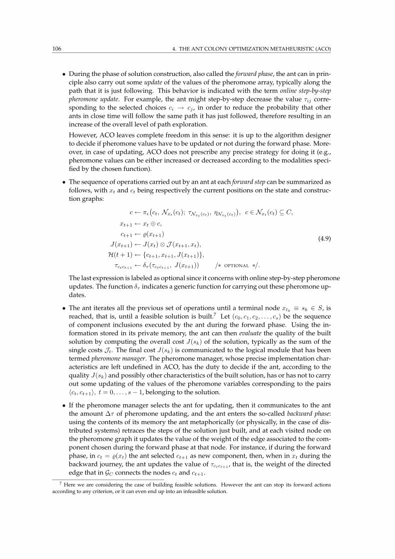
106 4. THE ANT COLONY OPTIMIZATION METAHEURISTIC (ACO)
• During the phase of solution construction, also called the forward phase, the ant can in prin-
ciple also carry out some update of the values of the pheromone array, typically along the
path that it is just following. This behavior is indicated with the term online step-by-step
pheromone update. For example, the ant might step-by-step decrease the value τij corre-
sponding to the selected choices ci → cj , in order to reduce the probability that other
ants in close time will follow the same path it has just followed, therefore resulting in an
increase of the overall level of path exploration.
However, ACO leaves complete freedom in this sense: it is up to the algorithm designer
to decide if pheromone values have to be updated or not during the forward phase. More-
over, in case of updating, ACO does not prescribe any precise strategy for doing it (e.g.,
pheromone values can be either increased or decreased according to the modalities speci-
fied by the chosen function).
• The sequence of operations carried out by an ant at each forward step can be summarized as
follows, with xt and ct being respectively the current positions on the state and construc-
tion graphs:
c← πǫ(
ct, Nxt(ct); τNxt
(ct), ηNxt(ct)
)
, c ∈ Nxt(ct) ⊆ C,
xt+1 ← xt ⊕ c,ct+1 ← (xt+1)
J(xt+1)← J(xt)⊗ J (xt+1, xt),
H(t+ 1)← ct+1, xt+1, J(xt+1),τctct+1
← δτ (τctct+1, J(xt+1)) /∗ OPTIONAL ∗/.
(4.9)
The last expression is labeled as optional since it concernswith online step-by-step pheromone
updates. The function δτ indicates a generic function for carrying out these pheromone up-
dates.
• The ant iterates all the previous set of operations until a terminal node xtk ≡ sk ∈ S, is
reached, that is, until a feasible solution is built.7 Let (c0, c1, c2, . . . , cs) be the sequence
of component inclusions executed by the ant during the forward phase. Using the in-
formation stored in its private memory, the ant can then evaluate the quality of the built
solution by computing the overall cost J(sk) of the solution, typically as the sum of the
single costs Jt. The final cost J(sk) is communicated to the logical module that has been
termed pheromone manager. The pheromone manager, whose precise implementation char-
acteristics are left undefined in ACO, has the duty to decide if the ant, according to the
quality J(sk) and possibly other characteristics of the built solution, has or has not to carry
out some updating of the values of the pheromone variables corresponding to the pairs
〈ct, ct+1〉, t = 0, . . . , s− 1, belonging to the solution.
• If the pheromone manager selects the ant for updating, then it communicates to the ant
the amount ∆τ of pheromone updating, and the ant enters the so-called backward phase:
using the contents of its memory the ant metaphorically (or physically, in the case of dis-
tributed systems) retraces the steps of the solution just built, and at each visited node on
the pheromone graph it updates the value of the weight of the edge associated to the com-
ponent chosen during the forward phase at that node. For instance, if during the forward
phase, in ct = (xt) the ant selected ct+1 as new component, then, when in xt during the
backward journey, the ant updates the value of τctct+1, that is, the weight of the directed
edge that in GC connects the nodes ct and ct+1.
7 Here we are considering the case of building feasible solutions. However the ant can stop its forward actionsaccording to any criterion, or it can even end up into an infeasible solution.
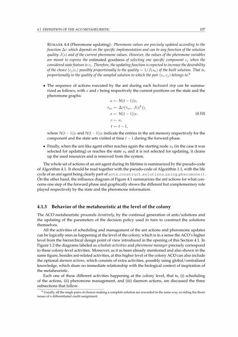
4.1 DEFINITION OF THE ACOMETAHEURISTIC 107
REMARK 4.4 (Pheromone updating): Pheromone values are precisely updated according to the
function ∆τ which depends on the specific implementation and can be any function of the solution
quality J(s) and of the current pheromone values. However, the values of the pheromone variables
are meant to express the estimated goodness of selecting one specific component cj when the
considered state feature is ci. Therefore, the updating function is expected to increase the desirability
of the choice (cj |ci) possibly proportionally to the quality ∼ 1/J(sk) of the built solution. That is,
proportionally to the quality of the sampled solution to which the pair (ci, cj) belongs to.8
• The sequence of actions executed by the ant during each backward step can be summa-
rized as follows, with x and c being respectively the current positions on the state and the
pheromone graphs:
κ← H(t− 1)|c,τκc ← ∆τ(τκc, J(sk)),
x← H(t− 1)|x,c← κ,
t← t− 1,
(4.10)
whereH(t− 1)|c andH(t− 1)|x indicate the entries in the ant memory respectively for the
component and the state sets visited at time t− 1 during the forward phase.
• Finally, when the ant-like agent either reaches again the starting node x0 (in the case it was
selected for updating) or reaches the state sk and it is not selected for updating, it cleans
up the used resources and is removed from the system.
The whole set of actions of an ant agent during its lifetime is summarized by the pseudo-code
of Algorithm 4.1. It should be read together with the pseudo-code of Algorithm 1.1, with the life
cycle of an ant agent being clearly part of ants construct solutions using pheromone().On the other hand, the influence diagram of Figure 4.1 summarizes the ant actions for what con-
cerns one step of the forward phase and graphically shows the different but complementary role
played respectively by the state and the pheromone information.
4.1.3 Behavior of the metaheuristic at the level of the colony
The ACO metaheuristic proceeds iteratively, by the continual generation of ants/solutions and
the updating of the parameters of the decision policy used in turn to construct the solutions
themselves.
All the activities of scheduling and management of the ant actions and pheromone updates
can be logically seen as happening at the level of the colony, which is in a sense the ACO’s higher
level from the hierarchical design point of view introduced in the opening of this Section 4.1. In
Figure 1.2 the diagrams labeled as schedule activities and pheromone manager precisely correspond
to these colony-level activities. Moreover, as it as been already mentioned and also shown in the
same figure, besides ant-related activities, at this higher level of the colony ACO can also include
the optional daemon actions, which consists of extra activities, possibly using global/centralized
knowledge, which share no immediate relationship with the biological context of inspiration of
the metaheuristic.
Each one of these different activities happening at the colony level, that is, (i) scheduling
of the actions, (ii) pheromone management, and (iii) daemon actions, are discussed the three
subsections that follow.8 Usually, all the single pairs of choices making a complete solution are rewarded in the same way, avoiding the thorn
issues of a differentiated credit assignment.
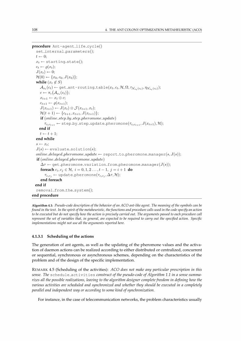
108 4. THE ANT COLONY OPTIMIZATION METAHEURISTIC (ACO)
procedure Ant-agent life cycle()
set internal parameters();
t← 0;
xt ← starting state();
ct ← (xt);
J(xt)← 0;
H(0)← x0, c0, J(x0);while (xt 6∈ S)
Axt(ct)← get ant-routing table(xt, ct,H,Ω, τNxt
(ct), ηNxt(ct));
c← πǫ(
Axt(ct))
;
xt+1 ← xt ⊕ c;ct+1 ← (xt+1);
J(xt+1)← J(xt)⊗ J (xt+1, xt);
H(t+ 1)← ct+1, xt+1, J(xt+1);if (online step by step pheromone update)
τctct+1← step by step update pheromone(τctct+1
, J(xt+1),H);
end if
t← t+ 1;
end while
s← xt;
J(s)← evaluate solution(s);
online delayed pheromone update← report to pheromone manager(s, J(s));
if (online delayed pheromone update)
∆τ ← get pheromone variation from pheromone manager(J(s));
foreach ci, cj ∈ H, i = 0, 1, 2 . . . , t− 1, j = i+ 1 do
τcicj← update pheromone(τcicj
,∆τ,H);
end foreach
end if
removal from the system();
end procedure
Algorithm 4.1: Pseudo-code description of the behavior of an ACO ant-like agent. The meaning of the symbols can befound in the text. In the spirit of the metaheuristic, the functions and procedure calls used in the code specify an actionto be executed but do not specify how the action is precisely carried out. The arguments passed to each procedure callrepresent the set of variables that, in general, are expected to be required to carry out the specified action. Specificimplementations might not use all the arguments reported here.
4.1.3.1 Scheduling of the actions
The generation of ant agents, as well as the updating of the pheromone values and the activa-
tion of daemon actions can be realized according to either distributed or centralized, concurrent
or sequential, synchronous or asynchronous schemes, depending on the characteristics of the
problem and of the design of the specific implementation.
REMARK 4.5 (Scheduling of the activities): ACO does not make any particular prescription in this
sense. The schedule activities construct of the pseudo-code of Algorithm 1.1 in a sense summa-
rizes all the possible realizations, leaving to the algorithm designer complete freedom in defining how the
various activities are scheduled and synchronized and whether they should be executed in a completely
parallel and independent way or according to some kind of synchronization.
For instance, in the case of telecommunication networks, the problem characteristics usually
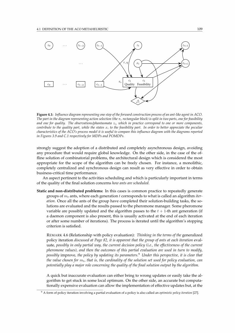
4.1 DEFINITION OF THE ACOMETAHEURISTIC 109
z0 · · · zt−2 zt−1 zt zt+1
· · · τ, η xt xt+1
c0 · · · ct−2 ct−1
πǫ ctQuality
ctFeasibility
Jt
Figure 4.1: Influence diagram representing one step of the forward construction process of an ant-like agent in ACO.The part in the diagram representing action selection (the πǫ rectangular block) is split in two parts, one for feasibilityand one for quality. The observations/phantasmata zi, which in practice correspond to one or more components,contribute to the quality part, while the states xi to the feasibility part. In order to better appreciate the peculiarcharacteristics of the ACO’s process model it is useful to compare this influence diagram with the diagrams reportedin Figures 3.9 and C.1 respectively for MDPs and POMDPs.
strongly suggest the adoption of a distributed and completely asynchronous design, avoiding
any procedure that would require global knowledge. On the other side, in the case of the of-
fline solution of combinatorial problems, the architectural design which is considered the most
appropriate for the scope of the algorithm can be freely chosen. For instance, a monolithic,
completely centralized and synchronous design can result as very effective in order to obtain
business-critical time performance.
An aspect pertinent to the activities scheduling and which is particularly important in terms
of the quality of the final solution concerns how ants are scheduled.
Static and non-distributed problems: In this cases is common practice to repeatedly generate
groups ofmt ants, where each generation t corresponds to what is called an algorithm iter-
ation. Once all the ants of the group have completed their solution-building tasks, the so-
lutions are evaluated and the results passed to the pheromone manager. Some pheromone
variable are possibly updated and the algorithm passes to the t + 1-th ant generation (if
a daemon component is also present, this is usually activated at the end of each iteration
or after some number of iterations). The process is iterated until the algorithm’s stopping
criterion is satisfied.
REMARK 4.6 (Relationship with policy evaluation): Thinking in the terms of the generalized
policy iteration discussed at Page 82, it is apparent that the group of ants at each iteration eval-
uate, possibly in only partial way, the current decision policy (i.e., the effectiveness of the current
pheromone values), and then the outcomes of this partial evaluation are used in turn to modify,
possibly improve, the policy by updating its parameters.9 Under this perspective, it is clear that
the value chosen for mt, that is, the cardinality of the solution set used for policy evaluation, can
potentially play a major role concerning the quality of the final solution output by the algorithm.
A quick but inaccurate evaluation can either bring to wrong updates or easily take the al-
gorithm to get stuck in some local optimum. On the other side, an accurate but computa-
tionally expensive evaluation can allow the implementation of effective updates but, at the
9 A form of policy iteration involving a partial evaluation of a policy is also called an optimistic policy iteration [27].
110 4. THE ANT COLONY OPTIMIZATION METAHEURISTIC (ACO)
same time, can dramatically reduce the number of generations, and, accordingly, of possi-
ble policy improvements. Unfortunately, in the general case, given limited computational
resources there is no an exact recipe to assign the optimal balance between the accuracy of
the evaluations, that is, the numbermt of ants per generation, and the frequency of policy
updatings, that is, the number of iterations. However, in the practice, ACO’s implementa-
tions seem to be quite robust to different “reasonable” choices concerning the value ofmt,
which is usually between 5 and 50.
Dynamic and distributed problems: Similar problems arise in the case of this class of prob-
lems, and in particular referring to telecommunication networks. However, in this case,
the ant generation is usually done in distributed and asynchronous way and there is no
notion of algorithm iteration. Each node generates ant agents according to some private
or common frequency generation ωt, and it can see the outcomes of only those ants which
pass through it. The main challenge in the case of online network problems like adaptive
routing, consists in the ability of the algorithm to adapt to the ever changing global traf-
fic patterns by using only local information. At this aim, it is clear that a high frequency
generation of ant agents would continually provide the nodes with large amounts of fresh
information on the global traffic patterns. However, if it is true that more agents means
more information, on the other hand, too many agents could easily congest the network
with control packets, producing in turn a negative effect on the transmission of data pack-
ets. Therefore, in this case too, a critical tradeoff problem is associated to the ant schedul-
ing process. Again, in practice ACO’s implementations (AntNet algorithms in particular)
seem to be rather robust to the actual frequency used.
ACO does not make any particular prescription on either the value of mt or ωt. However, it
is evident that these parameters can play an important role in terms of obtained performance.
4.1.3.2 Pheromone management
Pheromone management consists of all those activities directly related to pheromone updating,
like: authorize/deny ants to update pheromone, decrease the pheromone levels by mimicking natu-
ral evaporation processes, update pheromone according to the communications coming from the
daemon block (see below), update pheromone using global/centralized knowledge. From a logical
point of view pheromone management can be seen as under the control of a pheromone manager
process.10
In ACO pheromone updating can happen in the following ways:
• Online step-by-step;
• Online delayed;
• Offline.
The keywords “online” and “offline” are in relationship to the ant actions. “Online” indicates
the fact that pheromone is updated by the ant agent during its life cycle. The terms “step-by-
step” and “delayed” indicate respectively the update of pheromone while building and after
having built a solution. The modality “offline” refers to the fact that pheromone can be updated
offline with respect to the ant activities. Offline does not mean “after” the ant actions but carried
out by a component of the algorithm other than the ant agents.
Evaporation is an example of such offline updating. Evaporation usually consists in a contin-
uous process of decay of the levels of all the pheromone variables in the system, independently
10 The definition of a pheromone manager as a logical separate process within the ACO description, which was not inthe original ACO description, stems from the merge operator σ of ant programming [33, 34].
4.1 DEFINITION OF THE ACOMETAHEURISTIC 111
from their participation or not in generated solutions. For instance, the following operation is
often executed in the implementations at the beginning of each new iteration:
τij(t+ 1) = ρτij(t), ∀i, j ∈ 1, . . . , N, ρ ∈ [0, 1].
REMARK 4.7 (Pheromone evaporation): Pheromone evaporation can allow the colony of ant-like agents
to slowly forget the past history so that the colony can direct its search towards new directions without
being over-constrained by past decisions.
Also pheromone updates triggered by daemon processes have to be seen as offline updates.
For example, pheromone can be updated on the solution resulting from the application of a
problem-specific procedure of local search.
REMARK 4.8 (Pheromone manager activities): The three forms used in ACO for pheromone updating
are under the logical control of the pheromone manager which: (i) regulates the dynamics of the evapo-
ration processes, if any, (ii) decides which solutions, among those generated either by the ant agents or
daemon procedures, should and which should not trigger respectively online delayed or offline pheromone
updates, (iii) decides if the agents should make use of online step-by-step updates.
The practical implementation of the activities (i-iii) can be realized in a number of different
ways, according to the different characteristics of the problem. For instance, the use or not of
online step-by-step updates is usually decided at algorithm design time, and, accordingly, all
the agents can be just created with this property switched on or off. For what concerns online
delayed and offline updates, the ant agents and the daemon procedures can be seen as reporting
to the pheromone manager the solutions they have generated, together with their evaluation,
and the pheromone manager decides which solutions should or should not trigger a pheromone
update. That is, the pheromone manager can authorize or not pheromone updating for a built
solution on the basis of some filtering strategy. For instance, in several successful ACO imple-
mentations elitist strategies are applied: only the best solutions modify (or have a much greater
impact) on the pheromones. In Chapter 5 several practical examples of the different strategies
in use are shown and discussed.
Pheromone initialization
In spite of the fact that during the execution of an ACO algorithm pheromone is continually
updated according to a variety of possible schemes, the pheromone initialization strategy can also
significantly affect the final performance. At beginning of the execution, without any knowl-
edge a priori, all the possible decisions can be considered as equivalent. Accordingly, all the
pheromone variables can be conveniently initialized to the same common value. This would cre-
ate a uniform distribution of the decision probabilities in terms of pheromone values. However,
the possible decisions will be differentiated bymeans of the heuristic values η, which are usually
associated to the costsJ (ci|cj) comingwith the same definition of the optimization problem. Af-
ter the first agents have completed their solutions, and the solutions have been evaluated, the
pheromone levels will be updated to reflect the newly acquired knowledge. Subsequent agents
will therefore result biased towards the good decisions “discovered” so far (exploitation of the
past experience), but will also, at the same time, explore new alternatives because of the stochas-
tic component in their decision policy. The implemented mechanism is expected to be ergodic
in a sense, gradually getting independent from the specific initialization point.
112 4. THE ANT COLONY OPTIMIZATION METAHEURISTIC (ACO)
4.1.3.3 Daemon actions
To improve overall system efficiency, ACO algorithms can be enriched with extra capabilities
referred to as daemon actions. That is, problem-specific actions which are not carried out by or
strictly related to the actions of the ant agents. These are optional activities which share no or
little relationship with the biological context of inspiration of the metaheuristic and which, at
the same time, usually require some sort of centralized/global knowledge (in contrast with the
ant actions, which need only local information). In practice, daemon actions refer to problem-
specific extra activities which are not carried out by the ant agents, which do not make explicit
use of pheromone for construction building and which are not restricted to the use of local
information.
Daemon actions are often used to implement centralized actions which could not be per-
formed by single ants but which are know to be quite effective for the solution of the problem at
hand. Typical examples are the execution of problem-specific procedures of local search (see Ap-
pendix B), and the collection of global information, that can be used to update pheromone
over a solution which has not been sampled in the current iteration (e.g., to repeatedly update
pheromone over the best so far generated solution), or to authorize or not a specific ant to update
pheromone at the level of the pheromone manager.
The presence of the daemon component emphasizes the fact that, if additional knowledge or
tools which are specific to the problem under consideration are available, they can be profitably
used inside the metaheuristic. It does not really matter if their application is or is not “compli-
ant” to the general ant computing paradigm, as long as their application is feasible in practice.
In some sense, this is one of the main strengths of the metaheuristic, whosemodular and open ar-
chitecture can easily accommodate the inclusion of external modules, developed independently
of ACO itself. Actually, this aspect has greatly promoted the combined use of ACO and local
search procedures specific for the problem at hand. The excellent performance provided by this
sort of hybrid algorithms, often at the state-of-the-art (see Chapter 5), confirms both the feasibility
and the effectiveness of the approach. Appendix B discusses also the good theoretical reasons
behind the combined use of construction and modification approaches.
4.2 Ant System: the first ACO algorithm
The next chapter provides an extensive review and discussion of ACO implementations in the
domains of both static and dynamic combinatorial optimization. However, a special position in
the ACO’s universe is undoubtly occupied byAnt System (AS), which was the first instance of an
ACO algorithm, developed by Marco Dorigo and his co-workers in 1991 [135, 144]. AS was de-
signed as a set of three ant-colony-inspired algorithms for TSP differing for the way pheromone
variables were updated by ants. Their names were: ant-density, ant-quantity, and ant-cycle. A
number of ant algorithms, including the ACO meta-heuristic itself, have later been inspired by
ant-cycle, the most performing of the three.11 Ant System can be seen as the original specimen
of ACO implementations, in particular for what concerns the application to “classical” combina-
torial problems. Therefore, AS is described here, rather than in the next chapter, to acknowledge
its special historical role and according to the fact that its characterizing traits are actually com-
mon to a number of other ACO algorithms and are in a sense “didactic” to introduce practical
implementations of the rather general framework introduced so far.
Algorithm 4.2 shows in pseudo-code the activities of an AS ant agent during its life cycle. The
11 Hereafter, as it has been done in most published papers, Ant System is identified with ant-cycle.

4.2 ANT SYSTEM: THE FIRST ACO ALGORITHM 113
pseudo-code should be compared to that of Algorithm 4.1, which shows the general behavior of
an ACO ant, in order to immediately capture the specific design characteristics of AS.
procedure AS-ant-agent life cycle()
i← 0;
xi ← get starting city();
ci ← xi;
J(xi)← 0;
H(0)← x0, c0, J(x0);while (|xi| 6= N)
foreach cj ∈ Nxi(ci) do
aij ← ταij · ηβij ; /∗ ENTRIES OF THE ANT-ROUTING TABLE ∗/end foreach
c← apply AS stochastic decision rule(Axi(ci)); /∗ APPLICATION OF πǫ ∗/
xi+1 ← (xi, c);
ci+1 ← c;
J(xi+1)← J(xi) + J (ci+1|ci); /∗ SUM UP THE TRANSITION COSTS ∗/H(i+ 1)← ci+1, xi+1, J(xi+1);i← i+ 1;
end while
s← xi;
J(s)← J(xi) + J (c0|ci); /∗ ADDITION OF THE COST TO RETURN TO THE FIRST CITY ∗/foreach ci, cj ∈ H, i = 0, 1, 2 . . . , N − 1, j = i+ 1 do
τij ← τij + 1/J(s); /∗ UPDATE PHEROMONE ON EDGES BELONGING TO THE SOLUTION ∗/end foreach
removal from the system();
end procedure
Algorithm 4.2: Pseudo-code description of the behavior of an ant-like agent in Ant System [135, 144], the first ACOalgorithm, designed to attack N-city TSPs. The pseudo-code should be compared to that of Algorithm 4.1, describingthe general behavior of an ACO ant. α and β at line 9 are assigned constants.
The algorithm behavior can be informally described as follows. C is the set of cities, C =
c1, c2, . . . , cN, with |C| = N . A number m ≤ N of ants is positioned in parallel on m cities.
The ants’ start state, that is, the start city, can be chosen randomly by means of the function call
get starting city(). Each ant then enter a while cycle (program line 7 in the figure) which
lasts N iterations, that is, until a tour is completed. The process is iterated, with groups of m
ants/solutions generated at each iteration.
During each step an ant located on state xi and corresponding phantasma ci identified by
the last added city, reads the entries aij ’s of the feasible ant-routing table Axi(ci) (line 9) and
passes them to the stochastic decision policy πǫ which chooses the city c to add to the partial
solution to (line 11) on the feasible neighborhood of the current state. Then the ant moves to the
new state (line 12), updates the current phantasma (line 13), sum up the incurred cost (line 14),
and updates its memory (step 15). The memory is used together with the problem constraints to
define the feasible neighborhoods in the same simple way described by Example 4.1 (i.e., only
not already included cities can be considered, and in fact, in the original version of AS, the term
“tabu list” was used to represent the ant’s memory).
Once ants have completed a tour (which happens synchronously, given that during each
iteration of the while loop each ant adds a new city to the tour under construction), they evaluate
114 4. THE ANT COLONY OPTIMIZATION METAHEURISTIC (ACO)
the built solution (line 19), andmetaphorically retrace the same tour backward in order to update
the value of pheromone variables τij associated to the pair of cities included in their solution
(lines 20–21). Every ant in AS is authorized to update pheromone. This is a characterizing
aspect of AS, and at the same time one of its major weak points. No filtering is applied and the
whole sampled information is used. We will see in Subsection 4.3.2 the potential problems in
terms of too noisy goodness estimates with such an approach. One of the major improvements
brought in ACS, the direct successor of AS (described in Subsection 5.1.1), consisted precisely in
the fact that an elitist strategy has been used, such that pheromone is updated only on the best so
far solution.
For each ant k, at the end of the t-th iteration the value of pheromone is increased of a quan-
tity ∆τk equal to the quality 1/J(sk(t)) of the solution sk(t) built by the ant:
τij(t)← τij(t) + ∆τk(t), ∀ 〈ci, cj〉 ∈ sk(t), ∆τk(t) = 1/J(sk(t)), k = 1, . . . ,m. (4.11)
The amount of pheromone τij associated to pair (i, j) represents the learned desirability of
choosing city j when in city i, that is, the utility of including edge 〈ci, cj〉 in the solution in the
hope of eventually building a good solution. Pheromone is increased of an amount proportional
to the quality of the generated solution: the shorter the tour generated by an ant, the greater the
amount of pheromone it adds. This has the effect of making the issued choices becoming more
desirable for future ants proportionally to the quality of the solution they belonged to. As for
most of the ACO implementations, there is no per-pair credit assignment: all the city pairs be-
longing to a solution receive the same amount of pheromone depending on the overall quality of
the solution, in spite of the step of the construction process (i.e., the state) at which the decision
was issued.
Once the ant has updated the pheromone, it is removed from the system, and the associated
resources are made free. In AS all the ants update pheromone following the online delayed
scheme, while no step-by-step online pheromone updating happens (again, this was first intro-
duced in ACS).
At the end of each iteration, after all ants have completed their tours, the pheromone man-
ager systematically operates pheromone evaporation by decreasing all pheromone values accord-
ing to the following law:
τij(t)← (1− ρ)τij(t), ∀i, j ∈ 1, . . . , N, ρ ∈ (0, 1], (4.12)
where ρ is the pheromone decay coefficient. The initial amount of pheromone τij(0) is set to a
same small positive constant value τ0 on all arcs. This decrease is aimed at favoring exploration.
Since pheromone is always increased on the used city pairs, without evaporation it could easily
happen that the search would become highly constrained, with the ants ending up generating
always the same tours (a situation called stagnation).
No problem-specific daemon actions are performed. Although it would be straightforward
to add for instance daemon actions based on some form of local search; this has been done in
most of the ACO algorithms for TSP that have developed after AS (see next chapter).
The transition costs J (cj |ci) comes directly from the problem instance, and represents the
“distance” (which coincides with the physical distance, in the case of Euclidean TSPs) for travel-
ing from city ci to city cj . The local heuristic values ηij are precisely assigned using the inverse
of these distances between cities as defined by the problem instance. The parameters α and β
used in the ant-routing table’s functional form (line 9),
aij(t) = [τij(t)]α · [ηij ]β , (4.13)
serve to control the relative weight of pheromone (i.e., learned utility) and heuristic value (a pri-
ori local cost). Actually, this functional composition for pheromone and heuristic values became
4.3 DISCUSSION ON GENERAL ACO’S CHARACTERISTICS 115
quite popular, and it has been used over and over in ACO’s implementations. If α = 0, the
closest cities are more likely to be selected: this corresponds to a classical stochastic greedy algo-
rithm (with multiple starting points since ants are initially randomly distributed on the nodes).
If on the contrary β = 0, only pheromone amplification is at work: this method will likely lead
to the rapid emergence of a stagnation, with all ants making the same tour which, in general,
is strongly sub-optimal [146]. An appropriate trade-off has to be therefore set between heuristic
value and pheromone importance.
The values akij(t) of the ant-routing table for the k-th ant at iteration t are used by the stochas-
tic decision policy πǫ (function apply AS stochastic decision rule() at line 11) in the
following way. First, these values are normalized in order to obtain selection probabilities:
pkij(t) =akij(t)
∑
cn∈Nxk (ci)
akin(t), (4.14)
and then, after the generation of a uniformly distributed random number, the new component is
chosen inNxk(ci), according (proportionally) to these probabilities (random proportional scheme).
This probabilistic selection scheme is another fingerprint of AS, and in the following we will re-
fer to this overall strategy as the AS decision rule. It greatly favors diversification in the sampled
solutions, but at the same time limits intensification of the search in the sense of not being really
greedy with respect to the supposedly good local decisions. A more greedy strategy is imple-
mented in ACS, which adopts a pure ǫ-greedy policy: the local decision with the highest value
of pheromone is issued with a probability q0 ≈ 1, while an exploratory decision in the some AS
form is issued only with the small probability 1−q0. In order to avoid that all ants end up gener-
ating the same tour, ACS adds to AS’s online delayed pheromone updating, online step-by-step
pheromone decreasing. In this way, the probability that during an iteration the same locally
“best” decision is issued decreases proportionally to the number of times the same decision is
issued.
REMARK 4.9 (AS’s soundness): In a sense, AS is a quite elegant but at the same time “naive” approach:
solutions are repeatedly sampled, all solution outcomes are used to update statistics, decisions are taken
according to a random proportional scheme which is expected to implement a good tradeoff between diver-
sification and intensification. All these ingredients would likely work quite well if pheromone variables
were associated to state transitions, resulting in a form of Monte Carlo learning on the state space. Un-
fortunately, this cannot be the case for the class of problems at hand. Pheromone variables are associated
to phantasmata resulting in a drastic state aliasing. Therefore, a number of “adaptations” of the basic AS
scheme have been implemented over the years in order to cope more efficiently with the information loss
associated to the state→ phantasma transformation.12
4.3 Discussion on general ACO’s characteristics
4.3.1 Optimization by using memory and learning
ACO finds its roots in the pheromone-based shortest path behavior of ant colonies, with the
pheromone field playing the role of collective and distributed memory of the colony’s experi-
ences and biasing the decisions of the single ants. The pheromone array plays a similar role in
12 When pheromone can be associated to state transitions, the AS scheme appears as particularly suitable for use. Thisis the case of the the work of [76], which applies ACO to the solution of MDPs. In this case, the authors assume that theycan deal directly with the MDP states, such that the pheromone array becomes equivalent to a state transition utilityfunction whose value is estimated by repeated sampling. Interestingly, since in this case pheromone can be associateddirectly to states, some form of information bootstrapping can be meaningfully implemented, giving raise to an ACOusing temporal differences [413, 414].
116 4. THE ANT COLONY OPTIMIZATION METAHEURISTIC (ACO)
ACO, encoding memory of the generated solutions and being used in turn by the decision pol-
icy. ACO can be therefore termed a memory-based approach to optimization. In general terms, this
fact essentially means two things:
• Memory of past experience is used in order to optimize the search process.
• Multiple solutions are generated during execution time in order to dynamically gather use-
ful information to encode into the memory in the form of pheromone variables.
This general strategy arises the questions of what at a certain moment of the execution is
retained of the experience, that is, of the solutions generated so far, and how this experience is
used in turn to build new, and possibly better, solutions. The answer that ACO provides to
these questions in terms of pheromone variables is one of the central and likely most original
and successful aspects of the metaheuristic.
Generally speaking, the validity of the use of memory is subject to the fact that the set S
of the solutions defining the instance of the combinatorial problem presents some regularities
that can be identified and exploited through experience, that is, through repeated generation of
solutions. Clearly, if no regularities can be singled out, a pure random/exhaustive search are
the best strategy to follow. However, typical combinatorial problems do have some regularities
that can be in principle exploited, as it is suggested by both theoretical studies and the empirical
evidence that many structured algorithms can in general perform better than blind searches.
Memory can be stored and used in a variety of different ways. Restricting the focus to com-
binatorial optimization a notable example of memory-based approach is tabu search [199, 200], in
which memory is used to define prohibitions. In its original form, in tabu search all the generated
solutions are kept in memory in order to avoid to retrace already visited paths in the solution
space. This can be seen as a reasonable heuristic of quite general validity that can help to op-
timize the efficiency of sampled solution trajectories toward local optima. On the other hand,
ACO makes much stronger assumptions, in fact:
REMARK 4.10 (Use of memory): ACO makes use of memory with the aim of learning the values of a
small parameter set, the pheromone set, that are used by the decision policy to construct solutions. That
is, memory of the generated solutions is framed in the pheromone array, which associate a real value to
each solution component or pair of solution components. This means that not a whole solution is retained
into the memory, but rather all the single choices (cj | ci) making up the solution.
The state xs = (c0, c1, . . . , ct, ct+1, . . . , cs) representing a solution is broken up in the disjoint
sets of features 〈ct+1 | ct〉 associated to each separate decision issued while constructing the
solution. The τij associated to each conditional decision expresses the statistical estimate of how
good the decision 〈cj | ci〉 seems to be according to the quality of the solutions towhich the choice
has so far participated. In turn, at each construction step, after projecting the current solution
state xi to the phantasma identified by one component ci = (xi) of the state set, the τij values
are used to take the decision about the next component to include. Using the ant metaphor, it
can be said that the ant perceives its current state xt as the phantasma ci obtained through the
generating function of the representation, .
REMARK 4.11 (ACO’s fingerprint): This specific way of framing and using memory in a con-
structive scheme, as well as, the same assumption that the combination of memory and learning can be
fruitfully used to solve combinatorial problems, can be seen as the true fingerprints of ACO.
Figure 4.2 graphically summarizes ACO’s behavior emphasizing the role of pheromone in
terms of collective memory and the notion of learning the possibly optimal pheromone values
by solution sampling. The figure also shows the difference in size between the large solution set
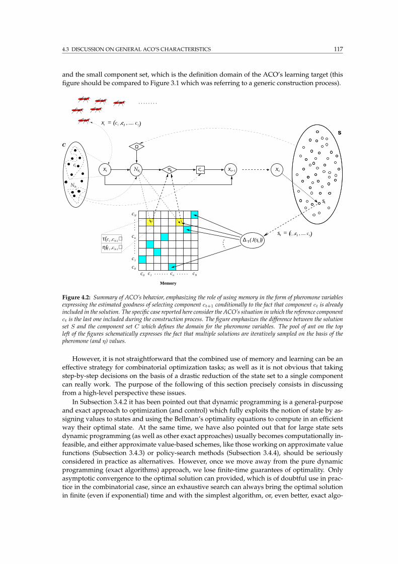
4.3 DISCUSSION ON GENERAL ACO’S CHARACTERISTICS 117
and the small component set, which is the definition domain of the ACO’s learning target (this
figure should be compared to Figure 3.1 which was referring to a generic construction process).
Ω
( )∆ ττ( ))η(
S
. . . . . . . .
ε
S
. . . . . . . . . . .
. . .
. .
. . .
. . .
Memory
ctN
tx
Nx t
xt xt+1 xs
c ,i ctc , .... js = (k cs)kJ(s )
cNcnc1c0
c0
c1
cn
cN
1c ,cN-1
cN-11c ,
c tc , .... j c tic ,tx = ( )
sk
C
t+1cπ
Figure 4.2: Summary of ACO’s behavior, emphasizing the role of using memory in the form of pheromone variablesexpressing the estimated goodness of selecting component ct+1 conditionally to the fact that component ct is alreadyincluded in the solution. The specific case reported here consider the ACO’s situation in which the reference componentct is the last one included during the construction process. The figure emphasizes the difference between the solutionset S and the component set C which defines the domain for the pheromone variables. The pool of ant on the topleft of the figures schematically expresses the fact that multiple solutions are iteratively sampled on the basis of thepheromone (and η) values.
However, it is not straightforward that the combined use of memory and learning can be an
effective strategy for combinatorial optimization tasks; as well as it is not obvious that taking
step-by-step decisions on the basis of a drastic reduction of the state set to a single component
can really work. The purpose of the following of this section precisely consists in discussing
from a high-level perspective these issues.
In Subsection 3.4.2 it has been pointed out that dynamic programming is a general-purpose
and exact approach to optimization (and control) which fully exploits the notion of state by as-
signing values to states and using the Bellman’s optimality equations to compute in an efficient
way their optimal state. At the same time, we have also pointed out that for large state sets
dynamic programming (as well as other exact approaches) usually becomes computationally in-
feasible, and either approximate value-based schemes, like those working on approximate value
functions (Subsection 3.4.3) or policy-search methods (Subsection 3.4.4), should be seriously
considered in practice as alternatives. However, once we move away from the pure dynamic
programming (exact algorithms) approach, we lose finite-time guarantees of optimality. Only
asymptotic convergence to the optimal solution can provided, which is of doubtful use in prac-
tice in the combinatorial case, since an exhaustive search can always bring the optimal solution
in finite (even if exponential) time and with the simplest algorithm, or, even better, exact algo-
118 4. THE ANT COLONY OPTIMIZATION METAHEURISTIC (ACO)
rithms like DP or branch-and-bound can provide the same result still in bounded exponential
time but “shorter”.13
In spite of the fact that in the general case only asymptotic properties can be proved, both
policy-search and approximate value-based methods have empirically shown to be usually able
to provide effective performance. As already remarked, ACO can be conveniently seen as a
form of policy search since it bypasses the direct assignment of values to states even if it retains
some notions of state (for feasibility) and the construction architecture typical of value-based
methods. The task faced by a policy-search algorithm is by no means easier than the original
combinatorial task, since it amounts to a search directly in the solution set. Therefore, specific
heuristics must be in order to search the solution set in some efficient way, trying to possibly
focus the search effort only to those parts containing the optimal solution. A typical way of
proceeding is by transforming the original problem into a possibly easier one and then solving
this easier problem in the hope that the optimal solution to this problem coincides with the
optimal solution of the original one. This is what precisely ACO does.
REMARK 4.12 (ACO transformation of the original problem into a low-dimensional learning
one): The search for s∗ ∈ S is carried out by looking for the optimal assignment of values of a small set of
real-valued parameters, the pheromone array τ , which are used as the parameters of the stochastic decision
policy πǫ controlling the processes of solution construction implemented by the ant-like agents. Therefore,
the original combinatorial problem is transformed into the problem of learning on the continuous set IRn
of dimension n = |C| ≪ |S|. So far, ACO’s implementation have not made use of approximators in the
sense of using compact representations of the state set (e.g., by using a neural network), therefore, ACO
can be said as based on a parametric lookup table representation.
That is, the search for good solutions is reduced to the search for an optimized decision policy
in the policy’s spaces. This global optimization problem is in turn reduced to a learning problem
by restricting the possible policies to a single parametric class of the type (see Equation 3.50):
πǫ(c|x; τ, η), c ∈ C, x ∈ X, τ, η ∈ T = IR|C|× IR|C|, (4.15)
defined over the component set, and depending on a set of assigned parameters, the heuristic
arrays, and a set of learning parameters, the pheromone array, both real-valued and of small
cardinality (with respect to the state set). The state information of the process is assumed as
available to the agents and is specifically used only for what concerns the feasibility of the so-
lutions. Each possible decision is associated to a pheromone variable, such that the pheromone
array results in a lookup table and every τij is intended as an estimate of the goodness of each
of the possible decisions. As pointed out in Subsection 4.3.1, this amounts to solve an MDP
whose states are the so-called phantasma, coinciding with the last component included in the
constructing solution. That is, amemoryless Markov model is built on top of the underlying exact state
model. In more precise terms, ACO is transforming the original problem (for what concerns qual-
ity optimization) into a POMDP whose characteristics are effectively described by the influence
diagram of Figure 4.1. In its original form ACO does not make any explicit use of state values,
such that this transformation of the original combinatorial problem into a learning problem over
a low-dimensional continuous space frames ACO into the class of policy search approaches, and,
13 These facts are in a sense the main reasons according to which hereafter the discussion is kept at a rather high-levellevel, without making, for instance, specific assumptions and derive very specific and possibly asymptotic mathematicalresult of dubious utility in practice. For us a metaheuristic is a tool that can allow to speed-up algorithm design whileat the same time obtaining good performance in practice for the problems of interest. Therefore, our objective here is topoint out where to frame ACO in the universe of the optimization strategies and where in general sense the “problems”are, in order to implicitly suggest possible general ways to overcome these same problems (possibly looking at solutionsproposed in the related frameworks). It is clear that more specific reasoning cannot be followed without restricting theclass of considered problems, that is, taking into account the specific characteristics of the different classes of problems.
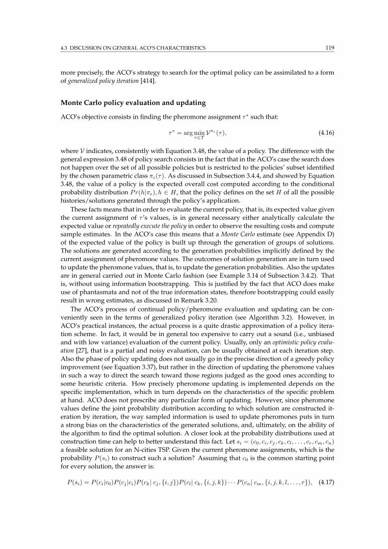
4.3 DISCUSSION ON GENERAL ACO’S CHARACTERISTICS 119
more precisely, the ACO’s strategy to search for the optimal policy can be assimilated to a form
of generalized policy iteration [414].
Monte Carlo policy evaluation and updating
ACO’s objective consists in finding the pheromone assignment τ∗ such that:
τ∗ = arg minτ∈TVπǫ(τ), (4.16)
where V indicates, consistently with Equation 3.48, the value of a policy. The difference with the
general expression 3.48 of policy search consists in the fact that in the ACO’s case the search does
not happen over the set of all possible policies but is restricted to the policies’ subset identified
by the chosen parametric class πǫ(τ). As discussed in Subsection 3.4.4, and showed by Equation
3.48, the value of a policy is the expected overall cost computed according to the conditional
probability distribution Pr(h|πǫ), h ∈ H , that the policy defines on the set H of all the possible
histories/solutions generated through the policy’s application.
These facts means that in order to evaluate the current policy, that is, its expected value given
the current assignment of τ ’s values, is in general necessary either analytically calculate the
expected value or repeatedly execute the policy in order to observe the resulting costs and compute
sample estimates. In the ACO’s case this means that a Monte Carlo estimate (see Appendix D)
of the expected value of the policy is built up through the generation of groups of solutions.
The solutions are generated according to the generation probabilities implicitly defined by the
current assignment of pheromone values. The outcomes of solution generation are in turn used
to update the pheromone values, that is, to update the generation probabilities. Also the updates
are in general carried out in Monte Carlo fashion (see Example 3.14 of Subsection 3.4.2). That
is, without using information bootstrapping. This is justified by the fact that ACO does make
use of phantasmata and not of the true information states, therefore bootstrapping could easily
result in wrong estimates, as discussed in Remark 3.20.
The ACO’s process of continual policy/pheromone evaluation and updating can be con-
veniently seen in the terms of generalized policy iteration (see Algorithm 3.2). However, in
ACO’s practical instances, the actual process is a quite drastic approximation of a policy itera-
tion scheme. In fact, it would be in general too expensive to carry out a sound (i.e., unbiased
and with low variance) evaluation of the current policy. Usually, only an optimistic policy evalu-
ation [27], that is a partial and noisy evaluation, can be usually obtained at each iteration step.
Also the phase of policy updating does not usually go in the precise direction of a greedy policy
improvement (see Equation 3.37), but rather in the direction of updating the pheromone values
in such a way to direct the search toward those regions judged as the good ones according to
some heuristic criteria. How precisely pheromone updating is implemented depends on the
specific implementation, which in turn depends on the characteristics of the specific problem
at hand. ACO does not prescribe any particular form of updating. However, since pheromone
values define the joint probability distribution according to which solution are constructed it-
eration by iteration, the way sampled information is used to update pheromones puts in turn
a strong bias on the characteristics of the generated solutions, and, ultimately, on the ability of
the algorithm to find the optimal solution. A closer look at the probability distributions used at
construction time can help to better understand this fact. Let si = (c0, ci, cj , ck, cl, . . . , cr, cm, cn)
a feasible solution for an N-cities TSP. Given the current pheromone assignments, which is the
probability P (si) to construct such a solution? Assuming that c0 is the common starting point
for every solution, the answer is:
P (si) = P (ci|c0)P (cj |ci)P (ck| cj , i, j)P (cl| ck, i, j, k) · · ·P (cn| cm, i, j, k, l, . . . , r), (4.17)

120 4. THE ANT COLONY OPTIMIZATION METAHEURISTIC (ACO)
that is, called xt the process state at step t-th:
P (si) = P (ci|c0)P (cj |ci)P (ck| cj , x1)P (cl| ck, x2) · · ·P (cn| cm, xN−1), (4.18)
where the conditional probabilities P (cv|cu, x) actually used are obtained from pheromone val-
ues after value normalization depending on the currently feasible neighborhood:
P (cv|cu, x) =τuv
∑
w∈Nx(cv) τuw. (4.19)
The potential problem lies in the fact that after an ant/solution has been selected for pheromone
updating, pheromone values are updated dropping off the state conditional component. For
each pair (u, v) the associated pheromone value expressing the learned desirability of having
such a pair in a solution is updated as P (cv|cu, x) would be the same as P (cv|cu), but unfortu-nately this is not the case. A choice cv ∈ N (cu) with associated pheromone value τuv actually
changes its probability P (v|u, x) of being selected when the phantasma is cu depending on the
other still feasible choices given the current state x. For instance, P (v|u, x) = 1 if Nx(cu) = v,but assumes the form 4.19 if |Nx(cu)| > 1, and quickly decreases as |Nx(cu)| gets large (e.g., at
the beginning of the solution construction for the case of a large problem). It must be pointed out
that this problem is common to most of the learning approaches to optimization based on the
estimation of and sampling from probability distributions. This issue will be further discussed
in Section 5.3. The following example, explained with the help of Figure 4.3 provocatively shows
how weird can in principle be the result of storing and using pheromone values which do not
carry enough state information.
EXAMPLE 4.3: EFFECTS OF MULTIPLE PHEROMONE ATTRACTORS
Let us consider the case of solutions expressed as sequences of length N = 10 and assume that only two
solutions, s1 and s2, with identical final cost Js have been generated so far, and both have been allowed to
update pheromone since Js is a good performance:
s1 = (c0, c1, c2, c3, c4, c5, c6, c7, c8, c9),
s2 = (c0, c9, c2, c1, c8, c3, c6, c5, c7, c4).
Therefore, on each pair (i, j) ∈ sk, k = 1, 2, τij will have a value possibly proportional to 1/Js. Notice
that (i, j) ∈ s1 ⇒ (i, j) 6= s2 and (i, j) ∈ s2 ⇒ (i, j) 6= s1. When a third solution is being constructed,
at each decision step there is an equal probability of choosing between a component pair included in either
s1 or s2. In a limit case (probability less than 0.002) the following solution can be obtained:
s3 = (c0, c1, c8, c9, c2, c3, c6, c7, c4, c5)
in which a pair from s1 is followed by a pair from s2 and vice versa. Therefore, in a sense, the solution
was built as the result of the actions of two competing attractors. The risk is that actually the alternating
attraction had completely disrupted the effective building blocks that had made the two original solutions
effective, possibly resulting in a solution of poor quality. Clearly, since pheromone is updated discarding
the full state information similar situations can in principle always happen.
The above effect of pheromone composition can be compared to that of the crossover operator in genetic
algorithms: s3 can be seen as constructed by the two “parents” s1 and s2 by alternating one component
from s1 and another from s2 when this meet the feasibility requirements.
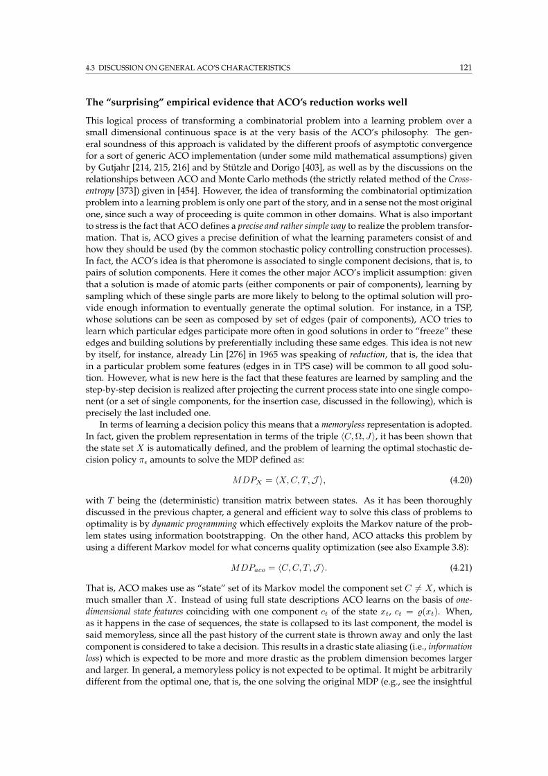
4.3 DISCUSSION ON GENERAL ACO’S CHARACTERISTICS 121
The “surprising” empirical evidence that ACO’s reduction works well
This logical process of transforming a combinatorial problem into a learning problem over a
small dimensional continuous space is at the very basis of the ACO’s philosophy. The gen-
eral soundness of this approach is validated by the different proofs of asymptotic convergence
for a sort of generic ACO implementation (under some mild mathematical assumptions) given
by Gutjahr [214, 215, 216] and by Stutzle and Dorigo [403], as well as by the discussions on the
relationships between ACO and Monte Carlo methods (the strictly related method of the Cross-
entropy [373]) given in [454]. However, the idea of transforming the combinatorial optimization
problem into a learning problem is only one part of the story, and in a sense not the most original
one, since such a way of proceeding is quite common in other domains. What is also important
to stress is the fact that ACO defines a precise and rather simple way to realize the problem transfor-
mation. That is, ACO gives a precise definition of what the learning parameters consist of and
how they should be used (by the common stochastic policy controlling construction processes).
In fact, the ACO’s idea is that pheromone is associated to single component decisions, that is, to
pairs of solution components. Here it comes the other major ACO’s implicit assumption: given
that a solution is made of atomic parts (either components or pair of components), learning by
sampling which of these single parts are more likely to belong to the optimal solution will pro-
vide enough information to eventually generate the optimal solution. For instance, in a TSP,
whose solutions can be seen as composed by set of edges (pair of components), ACO tries to
learn which particular edges participate more often in good solutions in order to “freeze” these
edges and building solutions by preferentially including these same edges. This idea is not new
by itself, for instance, already Lin [276] in 1965 was speaking of reduction, that is, the idea that
in a particular problem some features (edges in in TPS case) will be common to all good solu-
tion. However, what is new here is the fact that these features are learned by sampling and the
step-by-step decision is realized after projecting the current process state into one single compo-
nent (or a set of single components, for the insertion case, discussed in the following), which is
precisely the last included one.
In terms of learning a decision policy this means that a memoryless representation is adopted.
In fact, given the problem representation in terms of the triple 〈C,Ω, J〉, it has been shown that
the state set X is automatically defined, and the problem of learning the optimal stochastic de-
cision policy πǫ amounts to solve the MDP defined as:
MDPX = 〈X,C, T,J 〉, (4.20)
with T being the (deterministic) transition matrix between states. As it has been thoroughly
discussed in the previous chapter, a general and efficient way to solve this class of problems to
optimality is by dynamic programming which effectively exploits the Markov nature of the prob-
lem states using information bootstrapping. On the other hand, ACO attacks this problem by
using a different Markov model for what concerns quality optimization (see also Example 3.8):
MDPaco = 〈C,C, T,J 〉. (4.21)
That is, ACO makes use as “state” set of its Markov model the component set C 6= X , which is
much smaller than X . Instead of using full state descriptions ACO learns on the basis of one-
dimensional state features coinciding with one component ct of the state xt, ct = (xt). When,
as it happens in the case of sequences, the state is collapsed to its last component, the model is
said memoryless, since all the past history of the current state is thrown away and only the last
component is considered to take a decision. This results in a drastic state aliasing (i.e., information
loss) which is expected to be more and more drastic as the problem dimension becomes larger
and larger. In general, a memoryless policy is not expected to be optimal. It might be arbitrarily
different from the optimal one, that is, the one solving the original MDP (e.g., see the insightful
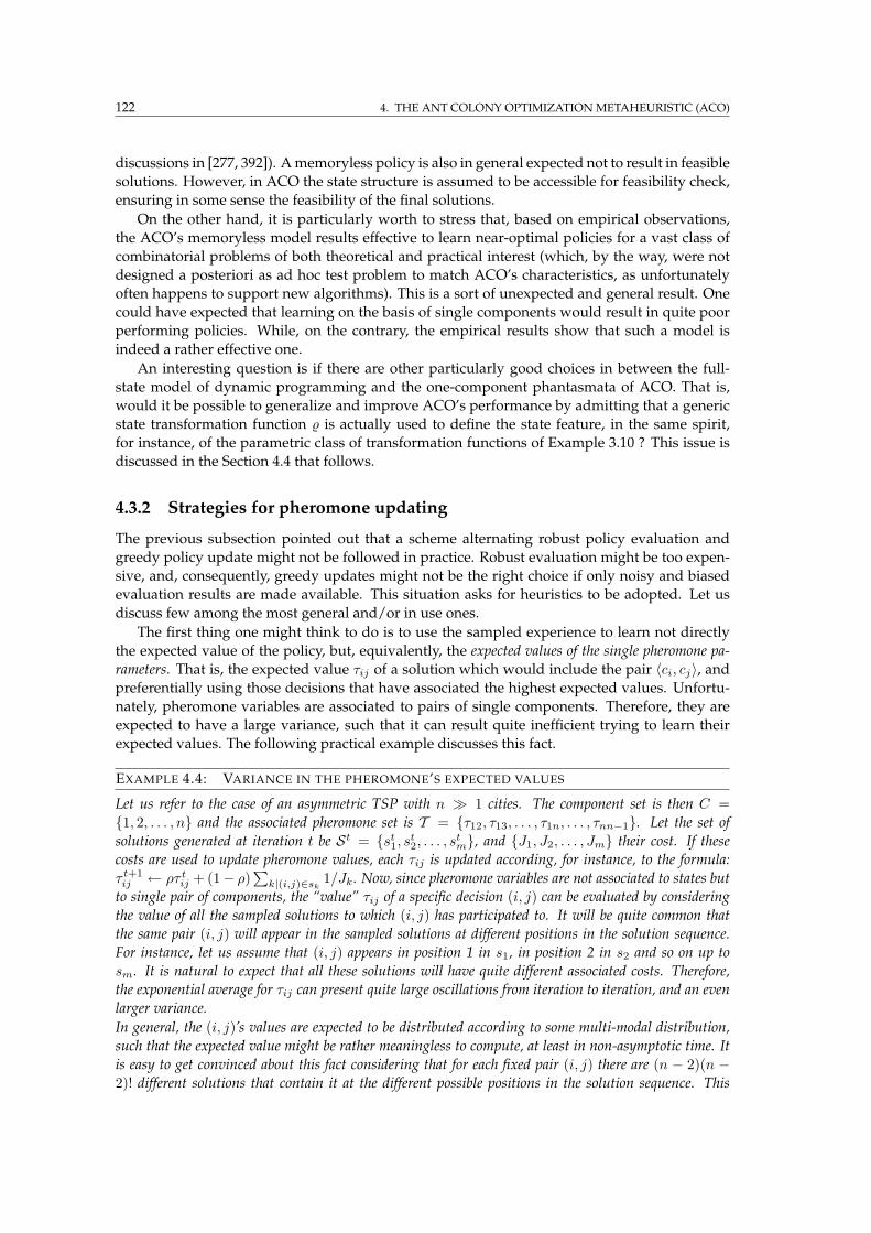
122 4. THE ANT COLONY OPTIMIZATION METAHEURISTIC (ACO)
discussions in [277, 392]). Amemoryless policy is also in general expected not to result in feasible
solutions. However, in ACO the state structure is assumed to be accessible for feasibility check,
ensuring in some sense the feasibility of the final solutions.
On the other hand, it is particularly worth to stress that, based on empirical observations,
the ACO’s memoryless model results effective to learn near-optimal policies for a vast class of
combinatorial problems of both theoretical and practical interest (which, by the way, were not
designed a posteriori as ad hoc test problem to match ACO’s characteristics, as unfortunately
often happens to support new algorithms). This is a sort of unexpected and general result. One
could have expected that learning on the basis of single components would result in quite poor
performing policies. While, on the contrary, the empirical results show that such a model is
indeed a rather effective one.
An interesting question is if there are other particularly good choices in between the full-
state model of dynamic programming and the one-component phantasmata of ACO. That is,
would it be possible to generalize and improve ACO’s performance by admitting that a generic
state transformation function is actually used to define the state feature, in the same spirit,
for instance, of the parametric class of transformation functions of Example 3.10 ? This issue is
discussed in the Section 4.4 that follows.
4.3.2 Strategies for pheromone updating
The previous subsection pointed out that a scheme alternating robust policy evaluation and
greedy policy update might not be followed in practice. Robust evaluation might be too expen-
sive, and, consequently, greedy updates might not be the right choice if only noisy and biased
evaluation results are made available. This situation asks for heuristics to be adopted. Let us
discuss few among the most general and/or in use ones.
The first thing one might think to do is to use the sampled experience to learn not directly
the expected value of the policy, but, equivalently, the expected values of the single pheromone pa-
rameters. That is, the expected value τij of a solution which would include the pair 〈ci, cj〉, andpreferentially using those decisions that have associated the highest expected values. Unfortu-
nately, pheromone variables are associated to pairs of single components. Therefore, they are
expected to have a large variance, such that it can result quite inefficient trying to learn their
expected values. The following practical example discusses this fact.
EXAMPLE 4.4: VARIANCE IN THE PHEROMONE’S EXPECTED VALUES
Let us refer to the case of an asymmetric TSP with n ≫ 1 cities. The component set is then C =
1, 2, . . . , n and the associated pheromone set is T = τ12, τ13, . . . , τ1n, . . . , τnn−1. Let the set of
solutions generated at iteration t be St = st1, st2, . . . , stm, and J1, J2, . . . , Jm their cost. If these
costs are used to update pheromone values, each τij is updated according, for instance, to the formula:
τ t+1ij ← ρτ tij + (1− ρ)∑k|(i,j)∈sk
1/Jk. Now, since pheromone variables are not associated to states but
to single pair of components, the “value” τij of a specific decision (i, j) can be evaluated by considering
the value of all the sampled solutions to which (i, j) has participated to. It will be quite common that
the same pair (i, j) will appear in the sampled solutions at different positions in the solution sequence.
For instance, let us assume that (i, j) appears in position 1 in s1, in position 2 in s2 and so on up to
sm. It is natural to expect that all these solutions will have quite different associated costs. Therefore,
the exponential average for τij can present quite large oscillations from iteration to iteration, and an even
larger variance.
In general, the (i, j)’s values are expected to be distributed according to some multi-modal distribution,
such that the expected value might be rather meaningless to compute, at least in non-asymptotic time. It
is easy to get convinced about this fact considering that for each fixed pair (i, j) there are (n − 2)(n −2)! different solutions that contain it at the different possible positions in the solution sequence. This
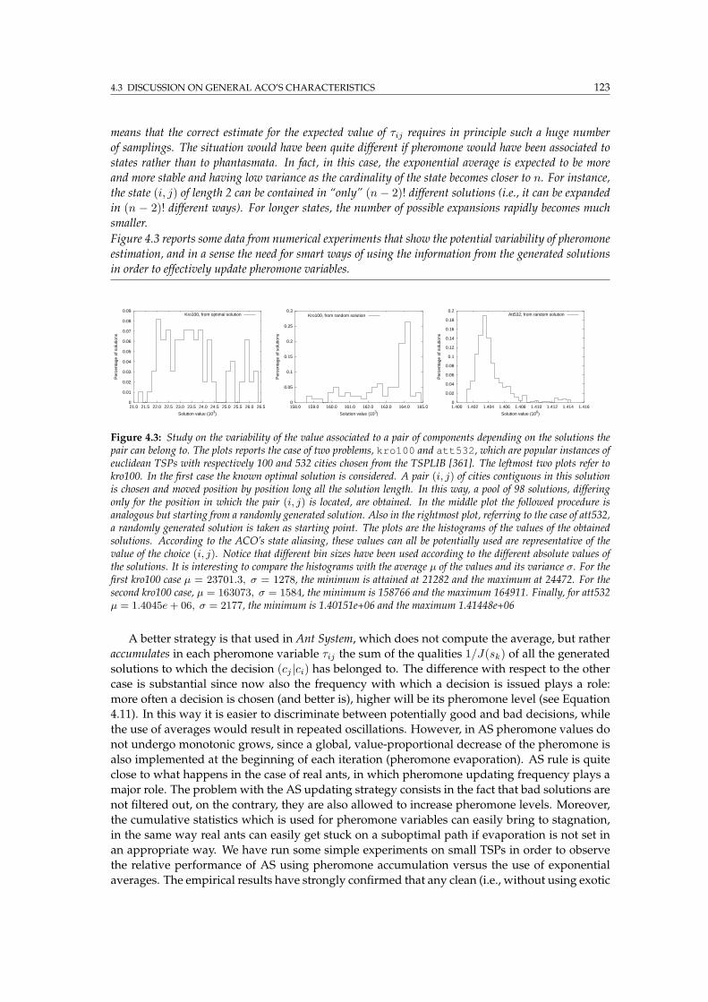
4.3 DISCUSSION ON GENERAL ACO’S CHARACTERISTICS 123
means that the correct estimate for the expected value of τij requires in principle such a huge number
of samplings. The situation would have been quite different if pheromone would have been associated to
states rather than to phantasmata. In fact, in this case, the exponential average is expected to be more
and more stable and having low variance as the cardinality of the state becomes closer to n. For instance,
the state (i, j) of length 2 can be contained in “only” (n− 2)! different solutions (i.e., it can be expanded
in (n − 2)! different ways). For longer states, the number of possible expansions rapidly becomes much
smaller.
Figure 4.3 reports some data from numerical experiments that show the potential variability of pheromone
estimation, and in a sense the need for smart ways of using the information from the generated solutions
in order to effectively update pheromone variables.
0
0.01
0.02
0.03
0.04
0.05
0.06
0.07
0.08
0.09
21.0 21.5 22.0 22.5 23.0 23.5 24.0 24.5 25.0 25.5 26.0 26.5
Per
cent
age
of s
olut
ions
Solution value (103)
Kro100, from optimal solution
0
0.05
0.1
0.15
0.2
0.25
0.3
158.0 159.0 160.0 161.0 162.0 163.0 164.0 165.0
Per
cent
age
of s
olut
ions
Solution value (103)
Kro100, from random solution
0
0.02
0.04
0.06
0.08
0.1
0.12
0.14
0.16
0.18
0.2
1.400 1.402 1.404 1.406 1.408 1.410 1.412 1.414 1.416
Per
cent
age
of s
olut
ions
Solution value (106)
Att532, from random solution
Figure 4.3: Study on the variability of the value associated to a pair of components depending on the solutions thepair can belong to. The plots reports the case of two problems, kro100 and att532, which are popular instances ofeuclidean TSPs with respectively 100 and 532 cities chosen from the TSPLIB [361]. The leftmost two plots refer tokro100. In the first case the known optimal solution is considered. A pair (i, j) of cities contiguous in this solutionis chosen and moved position by position long all the solution length. In this way, a pool of 98 solutions, differingonly for the position in which the pair (i, j) is located, are obtained. In the middle plot the followed procedure isanalogous but starting from a randomly generated solution. Also in the rightmost plot, referring to the case of att532,a randomly generated solution is taken as starting point. The plots are the histograms of the values of the obtainedsolutions. According to the ACO’s state aliasing, these values can all be potentially used are representative of thevalue of the choice (i, j). Notice that different bin sizes have been used according to the different absolute values ofthe solutions. It is interesting to compare the histograms with the average µ of the values and its variance σ. For thefirst kro100 case µ = 23701.3, σ = 1278, the minimum is attained at 21282 and the maximum at 24472. For thesecond kro100 case, µ = 163073, σ = 1584, the minimum is 158766 and the maximum 164911. Finally, for att532µ = 1.4045e + 06, σ = 2177, the minimum is 1.40151e+06 and the maximum 1.41448e+06
A better strategy is that used in Ant System, which does not compute the average, but rather
accumulates in each pheromone variable τij the sum of the qualities 1/J(sk) of all the generated
solutions to which the decision (cj |ci) has belonged to. The difference with respect to the other
case is substantial since now also the frequency with which a decision is issued plays a role:
more often a decision is chosen (and better is), higher will be its pheromone level (see Equation
4.11). In this way it is easier to discriminate between potentially good and bad decisions, while
the use of averages would result in repeated oscillations. However, in AS pheromone values do
not undergo monotonic grows, since a global, value-proportional decrease of the pheromone is
also implemented at the beginning of each iteration (pheromone evaporation). AS rule is quite
close to what happens in the case of real ants, in which pheromone updating frequency plays a
major role. The problem with the AS updating strategy consists in the fact that bad solutions are
not filtered out, on the contrary, they are also allowed to increase pheromone levels. Moreover,
the cumulative statistics which is used for pheromone variables can easily bring to stagnation,
in the same way real ants can easily get stuck on a suboptimal path if evaporation is not set in
an appropriate way. We have run some simple experiments on small TSPs in order to observe
the relative performance of AS using pheromone accumulation versus the use of exponential
averages. The empirical results have strongly confirmed that any clean (i.e., without using exotic
124 4. THE ANT COLONY OPTIMIZATION METAHEURISTIC (ACO)
averaging rules) attempt of using pheromone in terms of averages does not produce appreciable
performance. However, in AS the fact that all the ants are permitted to update pheromone does
not allow to really single out those decisions which participate of the best solutions.
REMARK 4.13 (Elitist strategies go in the right direction): The empirical evidence seems to suggest
that the most effective strategies are those updating the policy parameters according to some elitist se-
lection (borrowing the term used in evolutionary computation), that is, on the basis of only a restricted
subset (typically the best ones) of the solutions generated so far. This is for instance the strategy adopted
by ACS [140, 141, 184],MMAS [406, 407, 408, 404] and also by the cross-entropy method which
shares some strong similarities with ACO (e.g., see its application for fast policy search [298]).
ACS is actually one of the best performing ACO instances: it is a state-of-the-art algorithm
over an extensive set of problem classes (TSP, VRP, SCS) and instances, while models based on
either ACS orMMAS are usually the best performing ACO algorithms. The rationale behind
this design choice finds its hidden roots in the fact that since ACO does not make use of states
as learning target. Accordingly, the information coming from solution sampling should not be
intended for building robust estimates of the expected values of pair of choices, but rather for
quickly spotting which are those decisions that belongs to good solutions and “fixing” them for
further solutions’ construction. In practice, it is important to to be in some sense greedy towards
good solutions, and let the agents explore more in depth the areas around the good solutions
found, possibly moving toward another area when a new better/good solution is found. This
is precisely what ACS does: pheromone is repeatedly increased only for those decisions which
have participated to the best solution so far. In this way, further solutions are sampled in the
“neighborhood” of such best solutions. If a new better solution is found, the neighborhood
is moved toward the new best solution, and so son. In this way, still maintaining a good ex-
ploratory level, the search is intensified around each new best solution. Unfortunately, this way
of proceeding has also some drawbacks that have to be taken care of: if a new better solution is
not found in the currently searched “neighborhood”, the algorithm can easily end up repeatedly
looking in more or less the same region without bringing any further improvement. Moreover, if
several new better solutions are quickly found, the pheromone could be increased for a number
of different decisions actually belonging to different solutions. This would determine a sort of
composition of the pheromone that can result in a sort of multiple and potentially conflicting
pheromone attractors at each decision step (see also Example 4.3). It is not obvious when and
if such a composition can be or not beneficial (even if it reminds of the building blocks’ compo-
sition realized by the crossover operator in genetic algorithms). Actually, ACS throws away all
the new best solutions found at each iteration but one. In this way the problem of uncontrolled
pheromone composition is bypassed, but at the same time a consistent amount of potentially
useful information is discarded. In the Conclusions and Future Work chapter some ideas are
provided about how to exploit in an effective way these good solutions.
Another quite general approach for pheromone updatingwhich is particularly worth tomen-
tion is the Meuleau and Dorigo’s combination of ACOwith the popular [313] stochastic gradient
descent (e.g., see [374]). In their ACO/SGD (initially designed for TSPs and later generalized for
any combinatorial problem in [152, 455]) the generated solutions are used to evaluate the policy
with respect to the directions of the gradient descent in the pheromone space, such that at each
iteration step the pheromone vector is greedily moved downward the gradient direction. Even-
tually, under mild mathematical assumptions and appropriate setting of the algorithm parame-
ters, a local optimum in the pheromone space is guaranteed to be reached. The likely principal
merit of this work has consisted in pointing out a general way (the gradient updating rule) of
dealing with the otherwise ill-defined issue of pheromone updating. Certainly, this was possible
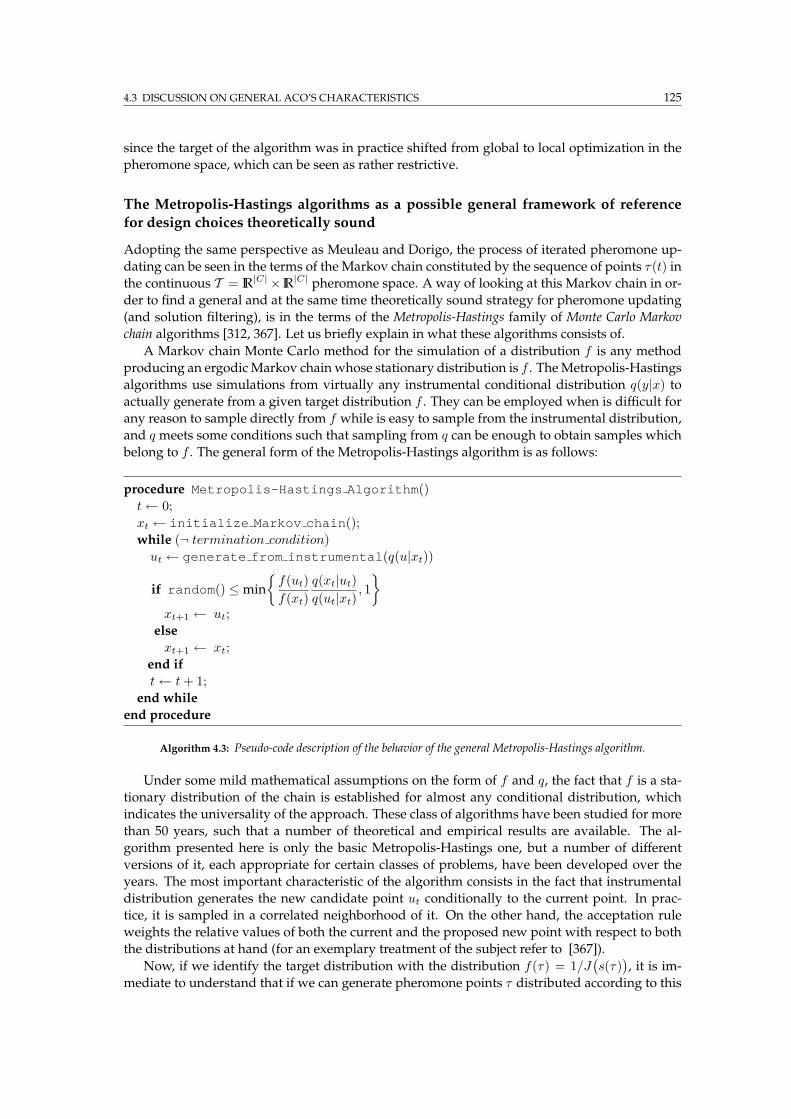
4.3 DISCUSSION ON GENERAL ACO’S CHARACTERISTICS 125
since the target of the algorithm was in practice shifted from global to local optimization in the
pheromone space, which can be seen as rather restrictive.
The Metropolis-Hastings algorithms as a possible general framework of reference
for design choices theoretically sound
Adopting the same perspective as Meuleau and Dorigo, the process of iterated pheromone up-
dating can be seen in the terms of the Markov chain constituted by the sequence of points τ(t) in
the continuous T = IR|C|× IR|C| pheromone space. A way of looking at this Markov chain in or-
der to find a general and at the same time theoretically sound strategy for pheromone updating
(and solution filtering), is in the terms of the Metropolis-Hastings family of Monte Carlo Markov
chain algorithms [312, 367]. Let us briefly explain in what these algorithms consists of.
A Markov chain Monte Carlo method for the simulation of a distribution f is any method
producing an ergodicMarkov chain whose stationary distribution is f . TheMetropolis-Hastings
algorithms use simulations from virtually any instrumental conditional distribution q(y|x) to
actually generate from a given target distribution f . They can be employed when is difficult for
any reason to sample directly from f while is easy to sample from the instrumental distribution,
and q meets some conditions such that sampling from q can be enough to obtain samples which
belong to f . The general form of the Metropolis-Hastings algorithm is as follows:
procedure Metropolis-Hastings Algorithm()
t← 0;
xt ← initialize Markov chain();
while (¬ termination condition)
ut ← generate from instrumental(q(u|xt))
if random() ≤ min
f(ut)
f(xt)
q(xt|ut)q(ut|xt)
, 1
xt+1 ← ut;
else
xt+1 ← xt;
end if
t← t+ 1;
end while
end procedure
Algorithm 4.3: Pseudo-code description of the behavior of the general Metropolis-Hastings algorithm.
Under some mild mathematical assumptions on the form of f and q, the fact that f is a sta-
tionary distribution of the chain is established for almost any conditional distribution, which
indicates the universality of the approach. These class of algorithms have been studied for more
than 50 years, such that a number of theoretical and empirical results are available. The al-
gorithm presented here is only the basic Metropolis-Hastings one, but a number of different
versions of it, each appropriate for certain classes of problems, have been developed over the
years. The most important characteristic of the algorithm consists in the fact that instrumental
distribution generates the new candidate point ut conditionally to the current point. In prac-
tice, it is sampled in a correlated neighborhood of it. On the other hand, the acceptation rule
weights the relative values of both the current and the proposed new point with respect to both
the distributions at hand (for an exemplary treatment of the subject refer to [367]).
Now, if we identify the target distribution with the distribution f(τ) = 1/J(
s(τ))
, it is im-
mediate to understand that if we can generate pheromone points τ distributed according to this
126 4. THE ANT COLONY OPTIMIZATION METAHEURISTIC (ACO)
target distribution we end up solving our optimization problem. In fact, this distribution assigns
the highest probabilities to the points with minimal cost value. If the J ’s optimum is not just an
isolated spike in the pheromone landscape, we might have a good probability to hit it. Any-
way, if q is defined in a proper way, the convergence of the Metropolis-Hastings algorithms will
guarantee the convergence in probability to the optimal solution in the sense of asymptotically
having a finite probability of generating it, probability whose value precisely depends on the
characteristics of the landscape.
Let us see which choices for q and f could be made in order to have a meaningful instance
of a general ACO in the terms of a Metropolis-Hastings algorithm. Since q should preferably be
chosen as a symmetric function (such that (q(x|u)/q(u|x) = 1), a good candidate appears to be
a Gaussian distribution. The new pheromone points will be therefore generated according to a
Gaussian centered in the current point. For the function f there is the problem of providing a
sound definition of the value f(τ), since eventually samples will be generated according to this
distribution. Several reasonable choices can be envisaged, each with different characteristics in
terms of convergence and finite time properties. A first choice might consist in taking as the
value returned by f(
τ(t))
the average of the quality of the m solutions generated at current it-
eration t according to the current τ(t) settings: f(τ(t)) =∑
m
(
J(sm(τ(t))))−1
/m. In this case,
f encodes the expected values associated to a pheromone assignment, which might not be what
we precisely want, since it will be likely very slow in practice. On the other hand, f can be like in
ACS the value of the best of the solutions generated at the current iteration. A sound and com-
putationally efficient way to define f is in the terms of the value of the solution obtained being ǫ-
greedy with respect to the policy implemented by the current pheromone vector τ(t). With these
choices for q and f , we obtain an algorithm which is an instance of ACO in which pheromone
is updated according to the values sampled from q and the current pheromone setting is either
accepted or rejected according to the result of its evaluation and of the stochastic Metropolis-
Hastings rule in which this value is used in turn. If q is a Gaussian, the next pheromone point
will be selected in some meaningful neighborhood of the current pheromone value.
Designing an ACO algorithm in the terms of a Metropolis-Hastings one is not expected to be
efficient in practice. However, this is a clearly interesting direction to explore since: (i) the issue
of pheromone updating becomes quite well defined, and is easy to choose an appropriate distri-
bution, like a Gaussian one, which can guarantee that the desired stationary distribution will be
attained, and can also provide satisfactory performance in practice, (ii) the issue of filtering out
solutions for pheromone updating is also “solved” in a sense, since is the Metropolis-Hastings
stochastic rule that will decide about accepting or rejecting a pheromone modification, (iii) it
might be possible to prove the convergence for a vast number of ACO algorithms just relying
on the general convergence properties of Metropolis-Hastings algorithms, and, finally, (iv) since
50 years of practical and theoretical results are available, it might be not so hard to find some
particularly effective choices for all the involved elements that fit the class of problems at hand.
4.3.3 Shortest paths and implicit/explicit solution evaluation
The use of a construction approach has allowed to speak in terms of state trajectories on the state
graph and to express a combinatorial optimization problem in the terms of finding theminimum
cost trajectory (see Remark 3.8) on the sequential state graph. Accordingly, ACO can be seen as
a metaheuristic for solving shortest path problems.
However, even if in principle ACO can be applied to almost any instance of shortest path
problems with finite-horizon, it has not to be seen as a competitive alternative for all those
cases for which “classical” algorithms, that is, label correcting methods (e.g., Dijkstra-like algo-
rithms [131]), label setting methods (e.g., dynamic programming algorithms like Bellman-Ford [21,
173]), and rollout algorithms [28] (see also Section 5.3) can be applied with success. ACO must
4.3 DISCUSSION ON GENERAL ACO’S CHARACTERISTICS 127
be seen as a viable alternative to deal with all those shortest path problems whose characteris-
tics make in general hard, ineffective, or computationally infeasible the application of those just
cited methods. This might be the case of NP-hard problems, as well as the case of shortest path
problems arising in distributed and dynamic environments (e.g., network routing).14
As it has already been discussed in the Introduction, and will be further discussed in the
next chapter, ACO seems to be particularly appropriate to attack this second class of problems.
This evidence finds its general rationale in the fact that ACO has a multi-agent architecture and
is based on an adaptive learning approach, which are characteristics that intuitively well match
the distributed and dynamic nature of these problems. Moreover, reasoning on a more “philo-
sophical” level, ACO is expected to perform comparatively better in dynamic and distributed
contexts also because it has been designed after ant colony’s behaviors, which are in turn the
result of a long phylogenetic evolution addressed at optimizing (in some sense) the ability of
the ants of moving over shortest paths precisely in the distributed and dynamic environments
where they live.
There is also another, more technical, reason related to ants behavior that makes particularly
successful the ACO application to the solution of geographically distributed shortest path prob-
lems. In ACO solutions generated by ants provide feedback to direct the search of future ants
entering the system. This is done by two mechanisms. The first one, which is common to all
ACO algorithms, consists of an explicit solution evaluation. In this case some measure of the
quality of the solution generated is used to decide in which amount pheromone should be in-
creased/modified. The second one is the same kind of the implicit path evaluationwhich has been
discussed in Section 2.1, that is, the fact that if an ant chooses a shorter path then it is also the
first to lay pheromone and to bias the search of forthcoming ants. In this way, shorter paths are
updated more frequently and can in turn attract more ants. Clearly, this effect becomes visible
only if there is an appreciable different in traveling time (e.g., length) among the paths, that is, if
differential path length (DPL) is at work.
It turns out that in geographically distributed problems, like network problems, implicit so-
lution evaluation can play an important role. When in AntNet [116, 120] explicit solution evalua-
tion was switched off by setting the amount of pheromone deposited by ants to a constant value
independent of the cost of the path built by the ant, it was still possible to find good solutions
just exploiting the DPL effect. Clearly, coupling explicit and implicit solution evaluation (by
making the amount of pheromone deposited proportional to the cost of the solution generated)
can easily improve performance.
The distributed nature of nodes in routing problems allows the exploitation of the DPL ef-
fect in a very natural way, without incurring in any additional computational costs. This is due
both to the decentralized nature of the system and to the inherently asynchronous nature of
the dynamics of telecommunication networks. On the contrary, this is not the case in combi-
natorial optimization problems where the most natural way to implement ACO algorithms is
by a colony of synchronized ants, that is, ants that synchronously add elements to the solution
they are building. Of course, it would in principle be possible to have asynchronous ants also
in combinatorial optimization problems. The problem is that the computational inefficiencies
introduced by the computational overhead necessary to have independent, asynchronous ants
can outweigh the gains due to the exploitation of the DPL effect (this was the case, for example,
of the asynchronous implementation of an ACO algorithm for the TSP reported in [97]).
14 All these shortest path problems have actually finite-horizons and deterministic transitions. On the other hand,there is also a recent application of ACO by Chang, Gutjahr, Yang, and Park [76] for the solution of generic MDPs withterminal state, of the same type of those typically considered in the domain of reinforcement learning. It will be in-teresting to explore this research direction more in detail to see if the ACO’s domain of application can be effectivelyexpanded also to this class of problems which involve stochastic transitions and in principle infinite horizons.
128 4. THE ANT COLONY OPTIMIZATION METAHEURISTIC (ACO)
4.4 Revised definitions for the pheromone model and the ant-
routing table
The given definition of ACO is essentially conformal to that originally provided in [147, 138],
even if it gives a more precise definition of some aspects (e.g., the meaning of and the rela-
tionships among problem states, solution components, and pheromone variables), and intro-
duces also few new notions (e.g., the logical module of the pheromone manager which acts
very alike the selection operator of evolutionary algorithms, and the function which charac-
terizes pheromone variables in terms of state features and points out the amount of informa-
tion loss). Nevertheless, as already remarked, the given ACO definition has also some short-
comings in the sense that a number of implementations (mostly applications to set, scheduling,
and max constraint satisfaction problems) that have appeared after its publications do not pre-
cisely fit into the definition for what concerns the characteristics of the pheromone model and the
way pheromone information is used at decision time. This fact calls for a new definition of the
pheromone model, in order to provide more flexibility in the definition of the information used
to take decisions.
In the following of the section, the part of the ACO definition concerning the pheromone
model is revised, with the aim of letting those applications fitting into the new definition while
at the same time generalizing the way pheromone is defined and used. The new definition will
open the possibility to design ACO implementations making use of more state information at
dcision time.
We proceeds as follows: first, a discussion showing the general limits of the current pheromone
model is provided, then, the characteristics of the new model are introduced.
4.4.1 Limits of the original definition
ACO frames and makes use of memory in terms of pairs of components, with the pheromone
graph being the graphical representation of this behavior. At each construction step the current
state xt is projected through onto the node ct of the pheromone graph, corresponding to the
last included component. In ct a decision is taken according to the estimated goodness τctcj
of each feasible choice cj ∈ Nxt(ct) conditionally to the fact that the current phantasma is ct.
This scheme matches quite well the case of solutions that can be expressed as sequences, since
the last included component can be intuitively seen as the current pivot of the solution being
constructed. However, in the case of set, or, more in general, of strongly constrained problems,
or when the insertion operation is used, this way of proceeding appears inadequate, in the same
way the use of the construction graph was found inadequate to reason about these same classes
of problems (see Subsection 3.3.3). Let us show these facts by considering more in depth the two
distinct cases of using insertion and solving set or constraint satisfaction problems.
Insertion operation: In this case, the decision policy is expected to take into account the whole
set of xt’s components (though losing the ordering information), such that the actual phan-
tasma should be more correctly seen in the terms of:
ins(xt) = c1, c2, . . . , ct, (4.22)
where c1, c2, . . . , ct are the components already included in the state sequence xt. That is,
ins(xt) becomes a multi-valued mapping that puts each state in correspondence to multi-
ple nodes on the pheromone graph. The overall sequence information is lost, but not that
related to all the single components already included in the state (the multigraph defined
in Example 3.7 would be a representation of the construction process more adequate than
the construction graph) Nevertheless, in spite of the fact that the state projection function
4.4 REVISED DEFINITIONS FOR THE PHEROMONE MODEL AND THE ANT-ROUTING TABLE 129
takes a different form with respect to the extension case, the pheromone graph does not
need to be modified. Pheromone variables (and also the heuristic ones) still refer to pairs
of components, even if the state information used at decision time is in this case larger than
that associated to the single node on the pheromone graph. On the other hand, the policy
πǫ takes in this case a decision on the basis of an ant-routing table which is different from
that used so far. In fact, it is the result of the union of all the ant-routing tables associated
to each component already included into the solution:
Ainsxt=⋃
ci∈xt
Axt(ci) (4.23)
Set and constraint satisfaction problems: For these classes of problems theremight be no really
good reasons to attribute a special role to the last included component, since there is no
explicit notion of ordering in the solutions. Therefore, the use of (xt) = ct, with ct being
the last included component, is likely to be of little efficacy for optimization purposes. A
more informative state feature should be reasonably chosen in order to obtain really good
performance. Rather than using as a reference the last included component, it might be
more sound to discard the whole state information and take decisions according to the
estimated goodness τ i of each feasible component, and not of pairs of components. That
is, instead of taking decision conditionally to a phantasma of dubious utility derived from
the state, decisions can be taken according to the unconditional estimate of how good is to
introduce a certain component into the solution. This simple solution looks more sound
and efficient than that referring to the use of the last component, also considering the fact
that the size of the learning set is in this way much reduced, passing from |C|(|C| − 1)
to |C|. From the point of view of the pheromone graph, it can be said that in this case
pheromone variables are associated to nodes rather than to arcs, that is, pheromone variables
take the form τ i, and indicate the goodness of including component ci into the partial
solution, independently from the characteristics of the partial solution itself.
Although pheromone variables take the form τ i, the general assumption that ACO asso-
ciates pheromone to pairs of components can still hold once the function that puts in
relationship state and pheromone graphs is appropriately rewritten as:
set(xt) = c0 = ∅, (4.24)
where the empty component c0 plays the role of fictitious component. Expression 4.24
says that associating pheromone to single components can be seen as formally equivalent
to associating pheromone to pairs of components, once a fictitious reference component is
introduced. With this artifice, the pheromone graph assumes the form of a star with c0 at its
center and pheromone associated to the directed arcs from c0 to all the other components.
Another equivalent description is that in which the pheromone graph is fully connected,
and each arc incident to a cj from any other ci ∈ C, ci 6= cj , has associated the same value τ j
of pheromone: τij = τ j , ∀i, i 6= j. The equivalence between these two representations was
already discussed in Figure 3.7 in relationship to the possible use of construction graphs
for generic set problems.
4.4.2 New definitions to use more and better pheromone information
In the ACO pheromone model pheromone variables are associated to pairs of components. That
is, τij represents the estimated goodness of including component cj conditionally to the fact
that ci is the last component that has been included in the current state xt. However, the two
previous examples on insertion and set problems have pointed out that in some cases more state
130 4. THE ANT COLONY OPTIMIZATION METAHEURISTIC (ACO)
information might be necessary, and that the function (x) might be expected to represent in
general a more complex feature extraction from the state than just the last component.
We identify two main ways of extending and generalizing the original pheromone model
and the way pheromone variables are used at decision time: (i) associating pheromone variables
not to pairs (component, component) but, more in general, to pairs (phantasma, component), with
the phantasma that can represent any set of state features, and (ii) increasing the number of
pheromone variables that are taken into account at decision time and considering at the same
time some aggregate function of their values. In the case (i), (x) is modified such that x is
projected over a subset ζ ∈ Z of state features larger than the single, last, component. Learning
happens between pairs (ζ, c), ζ ∈ Z, c ∈ C. That is, ACO aims at learning the goodness of
selecting component c conditionally to the fact that the current phantasma (i.e., state features) is
ζ. On the other hand, in case (ii), learning might still happen between pairs of components, as in
the original definition, but this time at each decision step a number of components is considered
and some aggregate measure of the related pheromone information is used in the ant-routing table
in order to obtain effective “surrogates” of state information. In the original definition only one
pheromone variable is considered in the ant-routing table (see Equation 4.2). While the case (i)
might in general imply an increase in the number of pheromone variables (and, accordingly, an
increase in the complexity of the learning task), the case (ii) does not. On the contrary, it only
involves an increase of complexity in the way pheromone variables are used to take decisions.
New definition of the ant-routing table: increasing the amount of information con-
sidered at decision time by value aggregation
Let us start by discussing first the case (ii), that changes the definition of the ant-routing table
and allows to extend the ACO definition in order to properly account for all the current imple-
mentations.
Let us assume that pheromone variables are still associated to pairs of components but a
mapping (x) is defined in order to associate a subset of components to the current state:
new(x) = ζ, x ∈ X, ζ ⊆ x. (4.25)
new(x) extracts from the state x = (c0, c1, . . . , ct) the desired subset of components. That is,
new(x) defines a generic operation of feature extraction from the state, such that a subset of
state components is singled out. At state x, the decision concerning the next component to
include is now taken on the basis of this composite information made of a subset of components
new(x), |new(x)| ≥ 1. The new ant-routing table results from the composition of two functions,
fτ , fη : Zn+ → IR, of this subset of components:
Anewx (ζ) = fτ (τ ζc) fη(ηζc) | ζ = new(x) ⊆ x ∧ ∀c ∈ C(x), (4.26)
where τ ζc indicates the set of all pairs τij with ci ∈ (x), and cj = c being of one the components
that are still feasible given x. Equation 4.26 should be compared to the previous definition 4.2:
Ax(ci) = τij ηij , ∀cj ∈ N (ci). According to the new definition, the probability of selecting a
specific component cj ∈ C(x) when the state is x becomes:
p(
cj |x) =fτ (τ ζcj
) fη(ηζcj)
∑
cj∈C(x) fτ (τ ζcj) fη(ηζcj
), ζ = (x) ⊆ x (4.27)
With these new definitions, the pheromone variables τcicjare still associated to single or pairs
of components, but the number of components ci ∈ x that are taken into account at decision time is
now defined by (x), and is not anymore necessarily one (such that the last component does not
anymore play any special role). Moreover, the transition probability for each feasible component
4.4 REVISED DEFINITIONS FOR THE PHEROMONE MODEL AND THE ANT-ROUTING TABLE 131
cj is defined according to a function fτ that possibly combines all the τcicjin order to assign a
selection probability taking into account as much as possible of state information. In this way,
the overall complexity of the ACO learning task is not increased, since the number of parameters to
learn (i.e., the pheromone variables) is unchanged. On the other hand, what is changed is the
amount of state information, and, accordingly, the amount of pheromone information which is
used at decision time. The information contained in the original pheromone model is therefore
used in a possibly more effective way:
REMARK 4.14 (Taking decisions on the basis of aggregate information): Any subset ζ of the x’s
components can be used at decision time, and the related pheromone (heuristic) information can be aggre-
gated according to any function fτ (fη). Pheromone variables still represent the desirability of choosing
cj conditionally to the fact that ci is already in the solution. Nevertheless, with the new definition 4.2 for
the ant-routing-table, pheromone and heuristic information associated to each one of the components in
the solution are potentially taken into account and used as an aggregate to define the selection probability
of feasible components. In this way, the desirability of cj is calculated conditionally not to the single (last)
component, but according to a more complete picture depending on the current state.
Some examples, directly inspired by existing ACO implementations(see Chapter 5), can
help to clarify how to use in practice Equation 4.27 (in all the examples it is assumed that the
current state is x = (c0, c1, . . . , ct)). To these examples is necessary to add also the work of
Merkle and Middendorf [307] on the so-called pheromone summation rule which addresses pre-
cisely the same issues but restricted to the case of specific scheduling problems.
EXAMPLES 4.5: APPLICATIONS OF THE NEW DEFINITION OF THE ANT-ROUTING TABLE
TSP: In this case, if the extension operation is used, we might do not need to change the standard
pheromone model in which (x) = ct, fτ = ταij , and fη = ηβij . On the other hand, if the insertion
operation is used, (x) = c0, c1, . . . , ct, and a likely good choice for fτ (and, equivalently, for fη) is:
fcjτ = max
ci∈(x)τij , ∀cj ∈ C(x).
This is in the same spirit of the GACS algorithm of Louarn et al. [281, 282].
CSP: In (max) constraint satisfaction problems if the current state is not taken into account at decision
time it is likely that either a poor or infeasible solution is generated. On the other hand, state information
can be effectively taken into account by using an additive aggregate as follows:
fcjτ =
∑
ci∈(x)
τcicj, ∀cj ∈ C(x), (x) = c0, c1, . . . , ct.
This is the solution proposed in her Ant Solver by Solnon [397, 396, 429]. In this case the components
are defined as the pairs cki = (vi, vki ) of decision variables vi and value vki ∈ D(vi), |D(vi)| = ni ∈ IN.
According to this way of proceeding, for each feasible component the value of the pheromone variables
relating the feasible component to each state component are summed up in order to assign the selection
probabilities in a more state-aware fashion but letting unchanged the meaning of and number of pheromone
variables.
BPP: For bin packing problems, which are constrained set problems, Levine and Ducatelle [272, 271, 154]
have proposed a solution which is very similar to that just described for CSPs. The only difference relies
in the fact that actually the average of the pheromone values is considered instead of the sum:
fcjτ =
1
|(x)|∑
ci∈(x)
τcicj, ∀cj ∈ C(x), (x) = c0, c1, . . . , ct.

132 4. THE ANT COLONY OPTIMIZATION METAHEURISTIC (ACO)
In this case the solution components coincide with the value of the items still to pack into the bins.
New definition of the pheromone model: extending the domain of the pheromone
variables
So far we have increased the amount of state information which is used at decision time by in-
creasing the number of pheromone variables that are taken into account, and by admitting the
very possibility of using some aggregate measure of them in order to assign selection probabil-
ities that are more state-aware. Nevertheless, the definition of the pheromone variables is left
unchanged, they are assumed to be associated to pair of components. This way of proceeding
can be naturally complemented by extending the domain of definition of the pheromone vari-
ables, with a consequent increase of the overall number of pheromone variables. That is, the pheromone
model can be extended by associating pheromone variables to generic pairs (state features, com-
ponent), and not anymore to pairs (component, component). In this way, pheromone variables
represent the estimate goodness of selecting component cj conditionally to the fact that the cur-
rent state feature (or phantasma) is ζ = (x). In this way more state information can be taken
into account and possibly better decisions can be issued. On the other hand, with this choice the
cardinality of the pheromone set becomes potentially larger than |C|, and grows rapidly with
the cardinality of the sets that define the phantasma (see also the strictly related discussions of
Chapter 3 about the phantasma and the generating function of the phantasma representation).
EXAMPLES 4.6: APPLICATIONS OF THE NEW DEFINITION FOR THE PHEROMONE MODEL
The function n of Example 3.10 can be used to parametrically define the set of pheromone variables. In
fact, if xt = (c0, c1, . . . , ct−n, ct−n+1, . . . , ct), the phantasma is defined from:
n(xt) = ζt = (ct−n, ct−n+1, . . . , ct), (4.28)
and pheromone variables are associated to all the feasible pairs (n, c), c ∈ C. In this case the dimension
of the pheromone set grows exponentially with n. For instance, for n = 2 and in the case of a general
asymmetric problem, the cardinality |T | of the pheromone set becomes |T | = |C||C − 1|2|C|−2, which
has to be compared with |Z| = |C||C − 1| of the n = 1 ACO’s case. It is clear that for large problems
(|C| ≫ 1) using n > 1 can become quickly infeasible in practice.
Let us show now a case in which on the contrary the state is mapped on the empty set, that is, all the state
information is discarded at decision time. Let us consider the single machine total weighted tardiness
scheduling problem. For this class of problems, the component set is conveniently seen as the union of
two different types of elements: C = jobs ∪ pos, where “pos” means the position in the scheduling
sequence. However, in principle there is little exploitable dependence between pairs of jobs, while it makes
more sense to reason in terms of learning the desirability of adding job cji at position cpk, where the super-
scripts j and p stands respectively for jobs and position. Therefore, in this case, according to the fact that
the job can be added either at the end of the current sequence or inserted in any position, a rule similar to
that showed for the TSP case can be used. For instance, in the extension case:
fc
jiτ = τ
cpt c
ji, ∀cji ∈ Nx(cpt ), (x) = cpt .
On the other hand, if the component set is taken in terms of the pairs (job, pos), and the whole state
information is discarded:
fc
jiτ = τ
cji, ∀cji ∈ C(x).
4.4 REVISED DEFINITIONS FOR THE PHEROMONE MODEL AND THE ANT-ROUTING TABLE 133
In this case pheromone variables are associated to single and not pair of components (although, the pair is
actually in the same definition of the component), such that:
(x) = ∅.
This is the approach followed in their ACO implementation by den Besten et al. [108].
The two solutions suggested to extend and improve ACO are not mutually exclusive, such
that they can be combined. However, while there is a number of ACO instances that fit for-
mula 4.27, there are no instances or studies concerning the association of pheromone variables
to pairs of the type (set of state features, component), except for the case of the ANTS subclass of
ACO, defined by Maniezzo et al. [291, 293], which actually considers the full state information.
Nevertheless, it is our conviction that getting a better understanding of the properties of differ-
ent feature extraction mappings is a fundamental yet overlooked direction of research for ACO
(the work on ant programming [33, 34] has only pointed out the issue without reporting any ex-
perimental result). The challenge consists in finding the optimal tradeoff between increasing
computational complexity and possible improvement in performance, and the identification of
classes of mappings that can result effective for specific classes of problems. In the limit, if
state and phantasma coincide, ACO would make use of the same amount of information which
is handled by dynamic programming. In such a scenario the repeated Monte Carlo sampling
can allow to effectively build unbiased estimates of the values of the problem states, such that
a general improvement of performance in terms of quality of the obtained solutions is expected
with respect to the case in which the phantasma coincides with a single component. On the
other hand, also a dramatic increase in the demand of computing power can be also reasonably
expected in order to obtain low variance estimates.
REMARK 4.15 (Tradeoff between the use of states and single components): The open question is
if there it is any good choice in between the case of learning decisions conditionally to single components
and learning decisions conditionally to full state information.
One potential major problem related to the use of phantasmata consisting of large subset of
components is that each single state trajectory has a priori very little probability of being sam-
pled (e.g., in an asymmetric TSP case every state trajectory has an a priori sampling probability
equal to 1/n!, which is very little for large number of cities n). Accordingly, the probability of
passing by the same phantasma gets smaller and smaller as the phantasma becomes closer and
closer to the complete information state. Therefore, being very little the probability of hitting
over and over the same phantasma, the ACO approach is not expected to be effective. In fact, it
becomes harder and harder to build reliable estimates about the best decision to issue condition-
ally to the fact of being in a specific phantasma. This is also the reason why ACO is not expected
to perform really well in the case of functions with domain in IRn, n ≥ 1, since in the continuous
each specific trajectory is a set with associated a null measure.
On the other hand, in the mentioned ANTS case (see Chapter 5), which results in a sort of
stochastic branch-and-bound controlled by learned pheromone values, a strong heuristic compo-
nent is used, and it causes a dramatic reduction in the effective number of trajectories that can be
actually sampled. In this way, the coupling of little exploration with learning of the pheromone
values can still provide excellent results.
Similar issues have been considered in depth in the field of reinforcement learning to attack
POMDPs (see Appendix C.2) using a value-based strategy but relying on some approximation
of the underlying information states. For instance, eligibility traces are used in [280] as a way of
retaining some useful information from the past experience while using a memoryless approach
for the POMDP at hand.
134 4. THE ANT COLONY OPTIMIZATION METAHEURISTIC (ACO)
4.5 Summary
The contribution of this chapter has consisted in the formal definition of the ACO metaheuristic
and the in-depth discussion of its characteristics. The definition of the ACOmetaheuristic is cen-
tral for this thesis. All the rest of the chapters are about applications and study of the properties
of ACO.
ACO has been defined in the terms of a metaheuristic based on solution construction, re-
peated Monte Carlo generation of solutions, use of memory and learning to bias the sequential
processes of solution generation according to a scheme of generalized policy iteration, use of
pairs of pheromone variables to frame memory of generated solutions and to learn about ef-
fective decisions, characterization of the set of pheromone variables as a small subset of state
features.
The definition given is substantially conformal to that given byDorigo, Di Caro, and Gambardella
in the papers were ACO was first introduced [147, 138]. Nevertheless, it contains several novel-
ties: (i) it is formally more precise, (ii) introduces the notion of pheromone manager, (iii) makes
clearer the role played by all the different components, (iv) discloses the link between ACO and
the important and well-established frameworks of sequential decision making, dynamic pro-
gramming and reinforcement learning, (v) explicits the the methodological and philosophical
assumptions behind ACO in terms of characteristics of the pheromone model and usefulness
of learning by sampling, (vi) points out the relationship between the state of the construction
process and the amount of information which is used for memory and learning in the form of
pheromone variables, (vii) highlights the limits of the notion of construction graph.
The chapter has also provided in-depth discussions of the different aspects of themetaheuris-
tic, focusing in particular on the use of memory and learning for combinatorial optimization
tasks, on the efficacy of different strategies for updating pheromone variables (i.e., for using
experience to learn effective construction policies), and on the fact that, similarly to the ants in
Nature, ACO ants solve shortest path problems and can exploit both explicit and implicit forms
of path evaluation.
The use of memory and learning is at the very foundation of ACO. In fact, it has been char-
acterized as an approach that transforms the original combinatorial optimization problem into
a learning problem over a low-dimensional parametric space identified by the pheromone vari-
ables, and solves the transformed problem adopting a policy-search approach based on repeated
(and concurrent) Monte Carlo construction of solutions. It is not immediate to assess in general
terms the efficacy of such a general approach concerning finite-time performance, as it has been
discussed in relationship to the use of value-based (e.g., dynamic programming) methods re-
lying on full state information versus policy-search methods realying on state features (which
is ACO’s case). On the other hand, the empirical evidences discussed in the next chapter sug-
gest that the ACO approach is indeed an effective one. Moreover, the several proofs of con-
vergence [214, 403, 215, 216] (see also Table 5.4) provide some guarantee about the ability of
generating the optimal solution in asymptotic time.
Elitist strategies for the selection of the solutions that are used for pheromone updating, that
is, for updating the statistical estimates of the goodness of the possible decisions, are identified
as the most effective ones. Nevertheless, it has also been pointed out the need to get a more
precise understanding of this fact, since this design components seems to be one of the keys to
reach state-of-the-art performance.
In the last part of the chapter we have also proposed a revised and extended definition for the
pheromone model and for the so-called ant-routing table, which is used to combine pheromone
and heuristic information at decision time. The purpose of these new definitions is twofold.
From one side, we aimed at making ACOmore in general and effective in the sense of increasing
the amount and/or the quality of the information used at decision time (moving toward the use
4.5 SUMMARY 135
of full information states as in dynamic programming). From the other side, we wanted to have
at hand a definition able to include (most of) all the algorithms based onACO that have appeared
also after the 1999’s definition, since many of them presented few design characteristics that did
not precisely find their counterpart in the early definition. That is, in the same spirit of the a
posteriori synthesis of the 1999’s definition, the new definition is based on an abstraction and
genralization of the characteristics of current implementations.
The proposed revised definitions find their roots in the characterization of ACO in terms
of sequential decision processes and in the understanding of the relationships and differences
between ACO and dynamic programming in terms of information used at decision time. In the
original definition, pheromone variables τij are associated to pairs of solution components, in
the sense that they express the estimated goodness of choosing a component cj ∈ C to add to
the solution being constructed conditionally to the fact that component ci is the last component
that has been included to form the current state x. In the new definition, pheromone variables
are more generically associated to pairs constituted by a state feature and a solution component.
That is, they represent the learned goodness of choosing component cj when ζx is the set of
features associated to the current state x ∈ X , with ζx = (x), and is a chosen feature extraction
mapping. Moreover, while in the original definition the selection probability of each feasible
choice is calculated from the ant-routing table on the basis of one single pheromone variable, the
revised definition removes this constraint. At decision time multiple pheromone variables can
be taken into account, and selection probabilities can be more generically assigned on the basis
of any arbitrary function combining these values.
Next chapter shows how all the elements discussed in this chapter have been effectively
put into practice to attack a wide collection of combinatorial problems of both theoretical and
practical interest.

136 4. THE ANT COLONY OPTIMIZATION METAHEURISTIC (ACO)
CHAPTER 5
Application of ACO to combinatorial
optimization problems
In this chapter we list and review most of the current ACO implementations. We provide a
quite comprehensive overview of which problems have been considered so far, which specific
design solutions have been proposed for each class of problems, and which are the quality of the
obtained results. Clearly, given the quite high number of available implementations, it will not
be possible to review all of them. A selection has been made taking into account several criteria,
like: the historical relevance (e.g., either it has been the first implementation for a certain class of
problems or it represents a reference template for other implementations), the particularly good
level of performance, the use of some very specific and interesting design solutions, etc.
The effectiveness in practice and the general soundness of the different design choices is
discussed, such that at the end of the chapter the reader is expected to have at hand a quite
complete picture of what has been already tried out in the ACO’s domain, and which are the
best ingredients to design an effective ACO algorithm.
For each implementation the adopted pheromone model and the form of the stochastic deci-
sion policy are always pointed out, as well as the relationships with previous ACO algorithms.
In particular, it will be evident that some algorithms (mainly because they were historically the
firsts to introduce some particularly effective components or strategies) have played the role of
reference template, at the same time guiding and constraining the design choice of subsequent
implementations (constraining in the sense that sometimes it looks like some specific design
choices have been issued rather acritically just copying from previous algorithms). These refer-
ence algorithms can be readily identified in Ant System, which has been described in Section 4.2,
ACS [141, 140, 184], andMMAS [404, 406, 407, 408] for what concerns static and non-distributed
combinatorial problems, and AntNet [120, 122, 124] and ABC [381, 382] concerning telecommu-
nication network routing problems.
Table 5.2 listsmost of the current ACO applications to both static and dynamic non-distributed
combinatorial problems. Table 5.1 lists the application to adaptive routing problems in telecom-
munication networks. Parallel implementations are listed in Table 5.3, while Table 5.4 lists more
theoretically oriented works (e.g., convergence proofs, general properties).
In the following of the chapter the focus is on the discussion of the characteristics of the
algorithms listed in Tables 5.2 and 5.3. Communication networks applications will be discussed
in depth throughout the second part of the thesis.
Some of the algorithms listed in Table 5.4 are mentioned in Section 5.3,
The last part of the chapter is devoted to a short discussion on other approaches to combi-
natorial optimization which are related to ACO, in order to provide a rather complete picture
of both applications and relationships to other frameworks. This related work section has to be
seen as a more specific add-on to the contents of Chapter 3 where related approaches have been
discussed on a rather general level. Again, related work specific to telecommunication networks
is not considered here but rather in the chapters that follow, that are devoted to telecommunica-
tion networks issues.
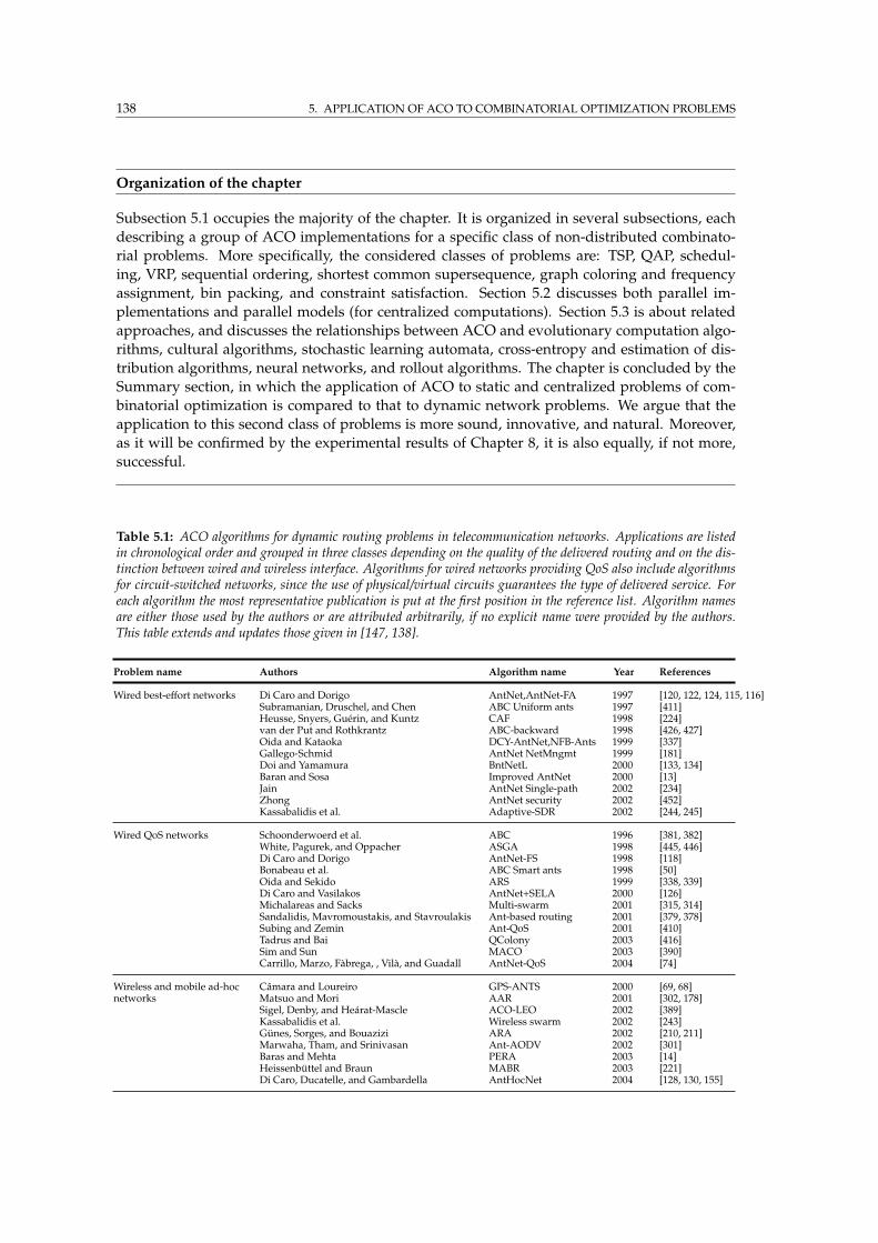
138 5. APPLICATION OF ACO TO COMBINATORIAL OPTIMIZATION PROBLEMS
Organization of the chapter
Subsection 5.1 occupies the majority of the chapter. It is organized in several subsections, each
describing a group of ACO implementations for a specific class of non-distributed combinato-
rial problems. More specifically, the considered classes of problems are: TSP, QAP, schedul-
ing, VRP, sequential ordering, shortest common supersequence, graph coloring and frequency
assignment, bin packing, and constraint satisfaction. Section 5.2 discusses both parallel im-
plementations and parallel models (for centralized computations). Section 5.3 is about related
approaches, and discusses the relationships between ACO and evolutionary computation algo-
rithms, cultural algorithms, stochastic learning automata, cross-entropy and estimation of dis-
tribution algorithms, neural networks, and rollout algorithms. The chapter is concluded by the
Summary section, in which the application of ACO to static and centralized problems of com-
binatorial optimization is compared to that to dynamic network problems. We argue that the
application to this second class of problems is more sound, innovative, and natural. Moreover,
as it will be confirmed by the experimental results of Chapter 8, it is also equally, if not more,
successful.
Table 5.1: ACO algorithms for dynamic routing problems in telecommunication networks. Applications are listedin chronological order and grouped in three classes depending on the quality of the delivered routing and on the dis-tinction between wired and wireless interface. Algorithms for wired networks providing QoS also include algorithmsfor circuit-switched networks, since the use of physical/virtual circuits guarantees the type of delivered service. Foreach algorithm the most representative publication is put at the first position in the reference list. Algorithm namesare either those used by the authors or are attributed arbitrarily, if no explicit name were provided by the authors.This table extends and updates those given in [147, 138].
Problem name Authors Algorithm name Year References
Wired best-effort networks Di Caro and Dorigo AntNet,AntNet-FA 1997 [120, 122, 124, 115, 116]Subramanian, Druschel, and Chen ABC Uniform ants 1997 [411]Heusse, Snyers, Guerin, and Kuntz CAF 1998 [224]van der Put and Rothkrantz ABC-backward 1998 [426, 427]Oida and Kataoka DCY-AntNet,NFB-Ants 1999 [337]Gallego-Schmid AntNet NetMngmt 1999 [181]Doi and Yamamura BntNetL 2000 [133, 134]Baran and Sosa Improved AntNet 2000 [13]Jain AntNet Single-path 2002 [234]Zhong AntNet security 2002 [452]Kassabalidis et al. Adaptive-SDR 2002 [244, 245]
Wired QoS networks Schoonderwoerd et al. ABC 1996 [381, 382]White, Pagurek, and Oppacher ASGA 1998 [445, 446]Di Caro and Dorigo AntNet-FS 1998 [118]Bonabeau et al. ABC Smart ants 1998 [50]Oida and Sekido ARS 1999 [338, 339]Di Caro and Vasilakos AntNet+SELA 2000 [126]Michalareas and Sacks Multi-swarm 2001 [315, 314]Sandalidis, Mavromoustakis, and Stavroulakis Ant-based routing 2001 [379, 378]Subing and Zemin Ant-QoS 2001 [410]Tadrus and Bai QColony 2003 [416]Sim and Sun MACO 2003 [390]Carrillo, Marzo, Fabrega, , Vila, and Guadall AntNet-QoS 2004 [74]
Wireless and mobile ad-hoc Camara and Loureiro GPS-ANTS 2000 [69, 68]networks Matsuo and Mori AAR 2001 [302, 178]
Sigel, Denby, and Hearat-Mascle ACO-LEO 2002 [389]Kassabalidis et al. Wireless swarm 2002 [243]Gunes, Sorges, and Bouazizi ARA 2002 [210, 211]Marwaha, Tham, and Srinivasan Ant-AODV 2002 [301]Baras and Mehta PERA 2003 [14]Heissenbuttel and Braun MABR 2003 [221]Di Caro, Ducatelle, and Gambardella AntHocNet 2004 [128, 130, 155]
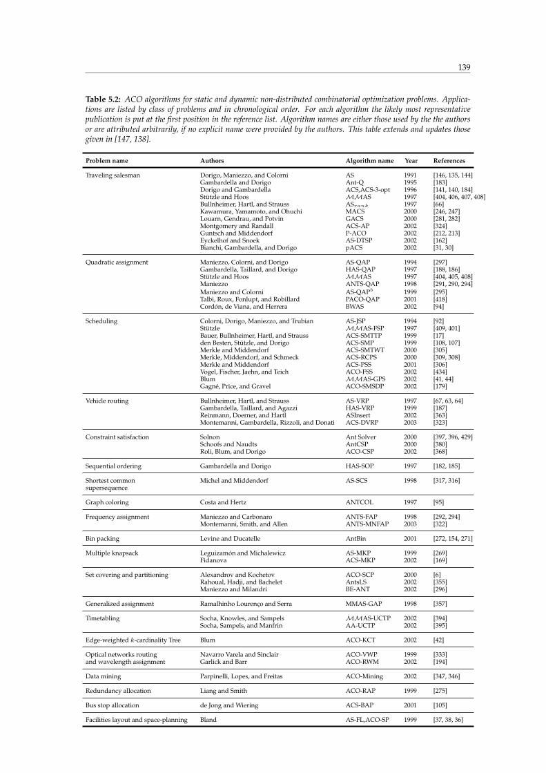
139
Table 5.2: ACO algorithms for static and dynamic non-distributed combinatorial optimization problems. Applica-tions are listed by class of problems and in chronological order. For each algorithm the likely most representativepublication is put at the first position in the reference list. Algorithm names are either those used by the the authorsor are attributed arbitrarily, if no explicit name were provided by the authors. This table extends and updates thosegiven in [147, 138].
Problem name Authors Algorithm name Year References
Traveling salesman Dorigo, Maniezzo, and Colorni AS 1991 [146, 135, 144]Gambardella and Dorigo Ant-Q 1995 [183]Dorigo and Gambardella ACS,ACS-3-opt 1996 [141, 140, 184]Stutzle and Hoos MMAS 1997 [404, 406, 407, 408]Bullnheimer, Hartl, and Strauss ASrank 1997 [66]Kawamura, Yamamoto, and Ohuchi MACS 2000 [246, 247]Louarn, Gendrau, and Potvin GACS 2000 [281, 282]Montgomery and Randall ACS-AP 2002 [324]Guntsch and Middendorf P-ACO 2002 [212, 213]Eyckelhof and Snoek AS-DTSP 2002 [162]Bianchi, Gambardella, and Dorigo pACS 2002 [31, 30]
Quadratic assignment Maniezzo, Colorni, and Dorigo AS-QAP 1994 [297]Gambardella, Taillard, and Dorigo HAS-QAP 1997 [188, 186]Stutzle and Hoos MMAS 1997 [404, 405, 408]Maniezzo ANTS-QAP 1998 [291, 290, 294]Maniezzo and Colorni AS-QAPb 1999 [295]Talbi, Roux, Fonlupt, and Robillard PACO-QAP 2001 [418]Cordon, de Viana, and Herrera BWAS 2002 [94]
Scheduling Colorni, Dorigo, Maniezzo, and Trubian AS-JSP 1994 [92]Stutzle MMAS-FSP 1997 [409, 401]Bauer, Bullnheimer, Hartl, and Strauss ACS-SMTTP 1999 [17]den Besten, Stutzle, and Dorigo ACS-SMP 1999 [108, 107]Merkle and Middendorf ACS-SMTWT 2000 [305]Merkle, Middendorf, and Schmeck ACS-RCPS 2000 [309, 308]Merkle and Middendorf ACS-PSS 2001 [306]Vogel, Fischer, Jaehn, and Teich ACO-FSS 2002 [434]Blum MMAS-GPS 2002 [41, 44]Gagne, Price, and Gravel ACO-SMSDP 2002 [179]
Vehicle routing Bullnheimer, Hartl, and Strauss AS-VRP 1997 [67, 63, 64]Gambardella, Taillard, and Agazzi HAS-VRP 1999 [187]Reinmann, Doerner, and Hartl ASInsert 2002 [363]Montemanni, Gambardella, Rizzoli, and Donati ACS-DVRP 2003 [323]
Constraint satisfaction Solnon Ant Solver 2000 [397, 396, 429]Schoofs and Naudts AntCSP 2000 [380]Roli, Blum, and Dorigo ACO-CSP 2002 [368]
Sequential ordering Gambardella and Dorigo HAS-SOP 1997 [182, 185]
Shortest common Michel and Middendorf AS-SCS 1998 [317, 316]supersequence
Graph coloring Costa and Hertz ANTCOL 1997 [95]
Frequency assignment Maniezzo and Carbonaro ANTS-FAP 1998 [292, 294]Montemanni, Smith, and Allen ANTS-MNFAP 2003 [322]
Bin packing Levine and Ducatelle AntBin 2001 [272, 154, 271]
Multiple knapsack Leguizamon and Michalewicz AS-MKP 1999 [269]Fidanova ACS-MKP 2002 [169]
Set covering and partitioning Alexandrov and Kochetov ACO-SCP 2000 [6]Rahoual, Hadji, and Bachelet AntsLS 2002 [355]Maniezzo and Milandri BE-ANT 2002 [296]
Generalized assignment Ramalhinho Lourenco and Serra MMAS-GAP 1998 [357]
Timetabling Socha, Knowles, and Sampels MMAS-UCTP 2002 [394]Socha, Sampels, and Manfrin AA-UCTP 2002 [395]
Edge-weighted k-cardinality Tree Blum ACO-KCT 2002 [42]
Optical networks routing Navarro Varela and Sinclair ACO-VWP 1999 [333]and wavelength assignment Garlick and Barr ACO-RWM 2002 [194]
Data mining Parpinelli, Lopes, and Freitas ACO-Mining 2002 [347, 346]
Redundancy allocation Liang and Smith ACO-RAP 1999 [275]
Bus stop allocation de Jong and Wiering ACS-BAP 2001 [105]
Facilities layout and space-planning Bland AS-FL,ACO-SP 1999 [37, 38, 36]
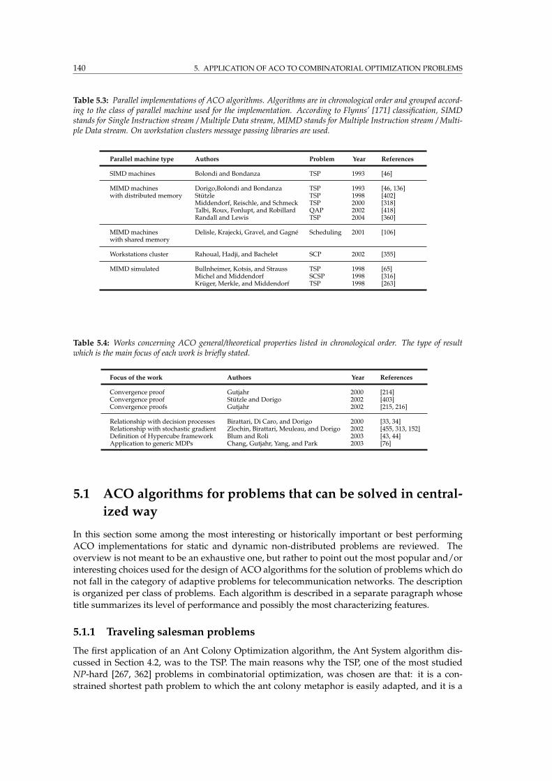
140 5. APPLICATION OF ACO TO COMBINATORIAL OPTIMIZATION PROBLEMS
Table 5.3: Parallel implementations of ACO algorithms. Algorithms are in chronological order and grouped accord-ing to the class of parallel machine used for the implementation. According to Flynns’ [171] classification, SIMDstands for Single Instruction stream / Multiple Data stream, MIMD stands for Multiple Instruction stream / Multi-ple Data stream. On workstation clusters message passing libraries are used.
Parallel machine type Authors Problem Year References
SIMD machines Bolondi and Bondanza TSP 1993 [46]
MIMD machines Dorigo,Bolondi and Bondanza TSP 1993 [46, 136]with distributed memory Stutzle TSP 1998 [402]
Middendorf, Reischle, and Schmeck TSP 2000 [318]Talbi, Roux, Fonlupt, and Robillard QAP 2002 [418]Randall and Lewis TSP 2004 [360]
MIMD machines Delisle, Krajecki, Gravel, and Gagne Scheduling 2001 [106]with shared memory
Workstations cluster Rahoual, Hadji, and Bachelet SCP 2002 [355]
MIMD simulated Bullnheimer, Kotsis, and Strauss TSP 1998 [65]Michel and Middendorf SCSP 1998 [316]Kruger, Merkle, and Middendorf TSP 1998 [263]
Table 5.4: Works concerning ACO general/theoretical properties listed in chronological order. The type of resultwhich is the main focus of each work is briefly stated.
Focus of the work Authors Year References
Convergence proof Gutjahr 2000 [214]Convergence proof Stutzle and Dorigo 2002 [403]Convergence proofs Gutjahr 2002 [215, 216]
Relationship with decision processes Birattari, Di Caro, and Dorigo 2000 [33, 34]Relationship with stochastic gradient Zlochin, Birattari, Meuleau, and Dorigo 2002 [455, 313, 152]Definition of Hypercube framework Blum and Roli 2003 [43, 44]Application to generic MDPs Chang, Gutjahr, Yang, and Park 2003 [76]
5.1 ACO algorithms for problems that can be solved in central-
ized way
In this section some among the most interesting or historically important or best performing
ACO implementations for static and dynamic non-distributed problems are reviewed. The
overview is not meant to be an exhaustive one, but rather to point out the most popular and/or
interesting choices used for the design of ACO algorithms for the solution of problems which do
not fall in the category of adaptive problems for telecommunication networks. The description
is organized per class of problems. Each algorithm is described in a separate paragraph whose
title summarizes its level of performance and possibly the most characterizing features.
5.1.1 Traveling salesman problems
The first application of an Ant Colony Optimization algorithm, the Ant System algorithm dis-
cussed in Section 4.2, was to the TSP. The main reasons why the TSP, one of the most studied
NP-hard [267, 362] problems in combinatorial optimization, was chosen are that: it is a con-
strained shortest path problem to which the ant colony metaphor is easily adapted, and it is a
5.1 ACO ALGORITHMS FOR PROBLEMS THAT CAN BE SOLVED IN CENTRALIZEDWAY 141
sort of didactic problem such that the algorithm behavior is not obscured by too many techni-
calities.
The fact that historically the first application of an ACO algorithm has been to the TSP has re-
sulted in many other implementations for this same class of problems. Some of these algorithms,
like the same Ant System, have become sorts of reference template that have been used in turn
to design ACO algorithms for different problems. Probably, the fact that the TSP is a kind of
didactic problem has facilitate the design of algorithms possessing quite well defined and clear
features that were easy to understand and to import into the design of new ACO algorithms.
Four algorithms in particular have brought ideas that have had amajor impact on subsequent
ACO algorithms for both TSP and other problems: Ant System, ACS, ACS-3-opt, and MAX–MIN Ant System. These algorithms (except for Ant System, already described) are discussed
in some detail in the following. Some other notable ACO implementations for the TSP are also
discussed, as well applications to dynamic and probabilistic versions of TSPs, which, in some
sense, are closer models of real-world situations.
All the following ACO implementations, and, more in general, the majority of ACO im-
plementations for TSP make use of the same pheromone model adopted in AS, consisting in
defining the set of the cities as the component set C = c0, c1, . . . , cN, the phantasma as the
last included component ct = (x) in the state sequence xt = (c0, c1, . . . , ct), and assigning ac-
cordingly pheromone variables in terms of pairs of cities. That is, τij represents the learned
desirability of choosing city cj ∈ Nx(ci) when ci is last component added to the state set.
Ant colony system (ACS), ACS-3-opt, andAnt-Q:major reference schemeswith state-
of-the-art performance
The Ant Colony System (ACS) algorithm has been introduced by Dorigo and Gambardella (1996)
[140, 141, 184] to improve the performance of AS, that was able to find good solutions within a
reasonable time only for small problems. In turn, ACS-3-opt improves the ACS’s performance
by including a daemon action based on an effective implementation of a problem-specific local
search procedure. ACS is based on AS but presents some important differences:
• ACSmakes use of a daemon procedure to update pheromone variables offline and accord-
ing to an elitist strategy: at the end of an iteration of the algorithm, once all the ants have
built a solution and reported it to the pheromone manager, pheromone is added only to
the decision pairs 〈ci, cj〉 used by the ant that found the best tour from the beginning of the
trial. In ACS-3-opt the daemon first activates a local search procedure based on a variant of
the 3-opt local search procedure [276] to improve the solutions generated by the ants and
then performs offline pheromone updates according to the following rule:
τij(t)← (1− ρ)τij(t) + ρ∆τij(t), 〈ci, cj〉 ∈ T+, (5.1)
where ρ ∈ (0, 1] is a parameter governing pheromone decay, ∆τij(t) = 1/J+, and J+ is the
length of T+, the best tour since the beginning of the trial. Equation 5.1 is applied only to
the pairs (i, j) belonging to T+. The ACS’s pheromone updating strategy 5.1 profoundly
differs from AS: a purely greedy strategy is used. Most of the sampled information is
actually discarded and only the pheromone associated to the best so far solution is re-
inforced/increased at each iteration. Every time a new best solution s+k (t+) is sampled,
pheromone is increased only for the decisions belonging to such solution, determining a
sort of new attractor in the pheromone space. In the next iteration, ants in a sense will
explore the neighborhood of such attractor (exploiting the online step-by-step pheromone
decreasing described below). Until a new best solution is not found, at the end of each new
iteration t > t+ the value of the pheromone variables corresponding to the pairs 〈c+i , c+j 〉
142 5. APPLICATION OF ACO TO COMBINATORIAL OPTIMIZATION PROBLEMS
which belonged to s+k (t+) is increased according to 5.1. Actually, the pheromone decrease
implemented by the ants online step-by-step, counterbalances the repeated pheromone in-
crease executed at the end of each iteration, such that the pheromone levels associated to
s+k (t+) result to be quite stationary from iteration to iteration. The two major negative as-
pects of this elitist strategy, consist in the fact that (i) if no new better solutions are sampled,
the search will not really move far away from the current attractor, only information about
the best solution is retained in colony’s memory, and, moreover, if several equally good
solutions are found at the same iteration, all but one are discarded in order to not incur in
the problems related to uncontrolled pheromone composition stressed in Example 4.3 and
Subsection 4.3.2.
• An ant k at state xi and associated phantasma ci chooses the city cj ∈ Nxi(ci) to move
to according to a decision policy implementing a so-called pseudo-random-proportional rule
which is a combination of the biased exploration strategy of AS with an ǫ-greedy policy.
Given q as a random variable uniformly distributed over [0, 1], and q0 ∈ [0, 1] a tunable
parameter, the pseudo-random-proportional rule is:
pkij(t) = 1 if q ≤ q0 and cj = arg maxcl∈Nxi(ci) ail,
pkij(t) = 0 if q ≤ q0 and cj 6= arg maxcl∈Nxi(ci) ail,
pkij(t) =akij(t)
∑
cl∈Nxi(ci)
akil(t)if q > q0,
(5.2)
where the ant-routing table aij is defined as in AS:
aij(t) =[τij(t)][ηij ]
β
∑
l∈Ni
[τil(t)][ηil]β∀j ∈ Nxi
(ci), (5.3)
This rule is such that an ǫ-greedy choice is issued with high probability (q0 ≈ 1), but
in order to favor also exploration, with a small probability the AS’s random proportional
rule (Equation 4.14) is also applied. Tuning q0 allows tomodulate the degree of exploration
and to choose whether to concentrate the activity of the system on the best solutions or to
explore more the search space.
• In ACS ants perform only online step-by-step pheromone updates. These updates are per-
formed to favor the emergence of other solutions than the best so far, counterbalancing
the greediness in the decision policy and the elitist strategy in pheromone updating. The
step-by-step pheromone updates are performed by applying the following rule:
τij(t)← (1− ϕ)τij(t) + ϕτ0 (5.4)
where 0 < ϕ ≤ 1. Equation 5.4 says that an ant moving from city ci to city cj ∈ Nxi(ci)
updates the pheromone value associated to the pair 〈ci, cj〉. The value τ0 is the same as
the initial value of pheromone trails and it was experimentally found that setting τ0 =
(NJNN )−1, where N is the number of cities and JNN is the length of a tour produced by
the nearest neighbor heuristic [195], produces good results. When an ant moves from city
ci to city cj , the application of the local update rule makes the corresponding pheromone
value τij diminish. The rationale for decreasing the pheromone on the path an ant is using
to build a solution is the following. Consider an ant k2 starting in city 2 and moving to
5.1 ACO ALGORITHMS FOR PROBLEMS THAT CAN BE SOLVED IN CENTRALIZEDWAY 143
city 3, 4, and so on, and an ant k1 starting in city 1 and choosing city 2 as the first city to
move to. Then, there are good chances that ant k1 will follow ant k2 with one step delay
given the ǫ-greedy decision policy 5.2. Decreasing the pheromone values by applying the
online step-by-step rule reduces the risk of such a situation. In other words, ACS’s local
update rule has the effect of making the used pairs 〈ci, cj〉 less and less attractive as they
are visited by ants, indirectly favoring the exploration of not yet issued decisions. As a
consequence, ants tend not to converge to a common path. This fact, which was observed
experimentally [141], is a desirable property given that if ants explore different paths then
there is a higher probability that one of them will find an improving solution than there is
in the case that they all converge to the same tour (which would make the use of m ants
pointless). On the other hand, this way of proceeding result in the fact that at each iteration
a neighborhood of the current best so far tour T+ is likely to be explored in order to find
improvements. Since in TSP is has been observed that local optima are usually grouped
together, this strategy is expected to be quite effective in practice.
• ACS exploits a data structure called candidate listwhich provides additional local heuristic
information, and which is a commonly used artifice in the TSP community when it comes
to deal with large problems. A candidate list is a list of preferred cities to be visited from a
given city. In ACS when an ant is in city ci, instead of examining all the unvisited neighbor
cities, it chooses the city to move to among those in the candidate list; only if no candidate
list city has unvisited status then other cities are examined. The candidate list of a city con-
tains cl cities ordered by increasing distance, where cl is a parameter, whose good values
seem to be around 15.
ACS was tested (see [140, 141] for detailed results) on standard problems, both symmetric
and asymmetric, of various sizes and compared with many other meta-heuristics. In all cases
its performance, both in terms of quality of the solutions generated and of CPU time required to
generate them, was the best one (a colony of 10 ants allowed to obtain the best results).
ACS-3-opt performance was compared to that of the genetic algorithm (with local optimiza-
tion) [177, 176] that won the First International Contest on Evolutionary Optimization [22]. The
two algorithms showed similar performance with the genetic algorithm behaving slightly better
on symmetric problems and ACS-3-opt on asymmetric ones.
ACS was actually the direct successor of Ant-Q (1995) [139, 183], an algorithm that tried to
merge AS and Q-learning [442] properties. In fact, Ant-Q differs from ACS only in the value
τ0 used by ants to perform online step-by-step pheromone updates. The idea was to update
pheromone trails with a value which was supposed to be a prediction of the value of the next
state, that is, identifying pheromone values with Q-values. In Ant-Q, an ant k at state xi imple-
ments online step-by-step pheromone updates by the following equation which replaces Equa-
tion 5.4:
τij(t)← (1− ϕ)τij(t) + ϕ γ maxl∈Nxi
(ci)τjl, γ ∈ [0, 1]. (5.5)
Unfortunately, it was later found that setting the complicate prediction term to a small constant
value, as it is done in ACS, resulted in approximately the same performance. Therefore, although
having a good performance, Ant-Q was abandoned for the equally good but simpler ACS. How-
ever, it must be notice that, in spite of the practical reasons that suggested the authors to abandon
Ant-Q, the ACO’s analysis done in the previous chapters clearly points out that the assump-
tions behind Equation 5.5 were quite wrong. In fact, the Q-learning rule, which is of the type:
Q(xt, ut)← Q(xt, ut)+ϕ[
J (xt+1|xt)+γmaxu∈C(xt)(xt+1, u)−Q(xt, ut)]
, or, in a formmore simi-
lar to that of Equation 5.5: Q(xt, ut)← (1−ϕ)Q(xt, ut)+ϕ[
J (xt+1|xt)+γmaxu∈C(xt)Q(xt+1, u)]
is based on the facts: (i) the x’s are states, such the equivalent of Bellman’s equations 3.36 hold for
144 5. APPLICATION OF ACO TO COMBINATORIAL OPTIMIZATION PROBLEMS
the Q-values, (ii) the Q-values precisely represent either costs-to-go or accumulated costs (see the
discussion at Subsection 3.4.2). In fact, Q-learning is actually an efficient way for solving MDPs
when the model of the Markov environment is not precisely known (in which case dynamic pro-
gramming would provide the optimal solution). Unfortunately, none of these properties hold
for pheromone variables, making rather questionable their use in the form of Equation 5.5.
Also other versions of ACSwere studiedwhich differ from the one described here because of:
(i) the way online step-by-step pheromone updates was implemented (in [141] experiments were
run disabling it, or by setting the update term in Equation 5.4 to the value τ0 = 0), (ii) the way
the decision rule was implemented (in [183] the pseudo-random-proportional rule of Equation 5.2
was compared to the random-proportional rule of Ant System, and to a pseudo-random rule which
differs from the pseudo-random-proportional rule because random choices were done uniformly
random), and (iii) the type of solution used by the daemon to update the pheromone values (in
[141] the use of the best solution found in the current iteration was compared with ACS’s use
of the best solution found from the beginning of the trial). ACS as described above is the best
performing of all the algorithms obtained by combinations of the above-mentioned choices.
MAX–MIN Ant System: elitist strategies, pheromone range and restarting
Stutzle andHoos (1997) [406, 407, 408, 404] have introducedMAX–MIN Ant System (MMAS),
which is based on AS, but: (i) an elitist strategy is used as in ACS since either only the best ant of
each iteration or the best ant so far are allowed to update pheromone variables, (ii) pheromone
values are restricted to an interval:
τij ∈ [τmin, τmax] ⊆ IR, ∀ci, cj ∈ C,
to avoid stagnation, (iii) pheromones are initialized to their maximum value τmax, and (iv) if the
algorithm does not generate a new best solution over a fixed number of iterations and most of
the pheromone values get close to τmin, a daemon component of the algorithm operates a restart
by reinitializing pheromone values and the value of the best so far tour to τmax.
Putting explicit limits on the pheromone values restricts the range of possible values for the
probability of including a specific edge into the solution. This helps avoiding stagnation, which
was one of the reasons why AS performed poorly even when an elitist strategy, like allowing
only the best ant(s) to update pheromone, was used (see [146]). To avoid stagnation, which
may occur in case some pheromone values are close to τmax while most others are close to τmin,
Stutzle and Hoos have added what they call a trail smoothing mechanism; that is, pheromone
values are updated using a proportional mechanism:
∆τij ∝ (τmax − τij(t)). (5.6)
In this way the relative difference between the pheromone values gets smaller, which obviously
favors the exploration of new paths. In practice,MMAS adds at the same time effective intensi-
fication (elitist strategy) and diversification (restricted range interval, restart and trail smoothing)
mechanisms to AS in order to overcome its major limits. According to the presented results, in
absolute terms withMMAS very high solution quality can be obtained. Moreover, MMAS
performs significantly better than AS, and slightly better than ACS. In particular, it shows better
performance than ACS for symmetric TSP instances, while ACS andMMAS reach the same
level of performance on ATSPs. The computational results with three variants ofMMAS sug-
gest that the best computational results are obtained when, in addition to the pheromone val-
ues limits, effective diversification mechanisms based on pheromone re-initialization are used.
While the idea of using a finite range for pheromone values quickly gained popularity within
ACO’s community, the idea of restart which was suggest by the authors as equally important,
apparently did not.
5.1 ACO ALGORITHMS FOR PROBLEMS THAT CAN BE SOLVED IN CENTRALIZEDWAY 145
ASrank: pheromone updating based on quality ranking
Bullnheimer, Hartl, and Strauss (1999) [66] proposed yet anothermodification of AS, calledASrank.
In ASrank the ants that at each iteration are allowed to update pheromone are chosen according
to the following strategy: (i) if Ji(t) is the length of the tour generated by the i-th ant at iteration
t, the m ants are ranked according to J ’s values and only the best σ − 1 ants in the ranking are
allowed to update pheromone on their tours, for an amount of pheromone proportional to the
ant rank, and (ii) the edges included in the best tour generated from the beginning of the trial
also receive additional pheromone scaled by σ (this is an elitist strategy logically carried out by
a daemon module). The overall dynamics for pheromone updating is given by:
τij(t)← (1− ρ)τij(t) + σ∆τ+ij (t) + ∆τ rij(t) (5.7)
where ∆τ+ij (t) = 1/J+(t), J+ being the length of the best solution from beginning of the trial,
and ∆τ rij(t) =∑σ−1µ=1 ∆τµij(t), with ∆τµij(t) = (σ − µ)1/Jµ(t) if the ant with rank µ has included
pair 〈ci, cj〉 in its tour and ∆τµij(t) = 0 otherwise. Jµ(t) is the length of the tour performed
by the ant with rank µ at iteration t. Equation 5.7 is applied to all pheromone array and im-
plements therefore both pheromone evaporation (the ρ factor), and online delayed and offline
pheromone updating. The authors found that their procedure improves significantly the quality
of the results obtained with AS.
GACS: making use of insertion strategy
TheGACS algorithm of Louarn, Gendrau, and Potvin (2000) [281, 282] is worthmentioning since
it is based on an insertion strategy rather than on the extension one which is adopted by the
majority of ACO implementations, and in particular by all the other algorithm discussed so far.
GACS, whose name comes from the combination of the “GENeralized Insertion” (GENI) heuris-
tic [197] and ACS, has design characteristics similar to those of ACS adapted to use insertion.
Differently from ACS, at state xt the new component cj to add is selected randomly among the
still feasible ones, then the insertion position is selected according to a rank-based scheme. First,
the ant-routing entries are computed as:
aij(t) =ηij
1 + γτij(t), ∀ci ∈ xt, (5.8)
where γ ∈ [0, 1] and τij is the value of pheromone normalized with respect to the highest value
of pheromone. Then, according to the aij ’s values, the possible insertion positions are ranked
and the precise location is selected according to a random selection over the ranks. GACS’s per-
formance versus ACS have been studied for a set of medium-sized problems from the TSPLIB.
The experimental results seem to indicate a clear superiority of GACS with respect to ACS.
P-ACO: population-based ACO for dynamic problems
Guntsch and Middendorf (2002) [212, 213] have proposed P-ACO, a population-based design
for ACO. In the usual ACO’s implementations pheromone values are the incremental result of
all the updates triggered by the pheromone manager since the start of algorithm execution. In
P-ACO, on the other hand, the pheromone patterns at time T are those precisely induced by
the current ant population P (t) and not the result of all past updates. That is, after one ant has
completed its solution, the ant is either added or included by replacement into the population set
according to both deterministic and stochastic criteria based on quality, population size, etc. (the
authors have explored several possibilities in this sense, also getting inspiration from the number
of population management techniques investigated in the field of evolutionary computation).
146 5. APPLICATION OF ACO TO COMBINATORIAL OPTIMIZATION PROBLEMS
If the ant enters the population, then the value of the pheromone variables associated to the
decisions issued by the ant are correspondingly increased according to an AS-like rule (Equation
4.11). On the other hand, if an ant/solution leaves the population (e.g., to make space to a
new better ant), then the corresponding pheromone is decreased of the same amount it was
increase when the ant entered the population. In this way, the pheromone values precisely
reflect the ants belonging to the current population P (t) at iteration t. In addition to this specific
mechanism, P-ACO makes use of the ACS’s pseudo-random-proportional rule (Equation 5.2)
for component selection but does not make any use of online step-by-step pheromone updates,
since pheromone updates are subject to the fact of either entering or leaving the population.
While the use of a population-based strategy to select which ants have to increase/decrease
pheromone might be of general usefulness, the authors conjecture that this approach is particu-
larly suitable for dynamic problems, where the problem instance changes over time. In particu-
lar, this is expected to be true when changes are not too severe and there exists a good heuristic
for modifying the solutions maintained in the population after a change, such that they can be-
come good solutions also for the modified problem. Since pheromone values do not depend
other than on the solutions in the population, it is not necessary to apply any additional mecha-
nism to adapt the pheromone information to the new situation.
P-ACO’s implementations have been applied to dynamic versions of both TSP and QAP
instances. The dynamic component being in the fact that cities/locations can be randomly in-
serted, replaced or deleted. A subset R of half of the cities/locations is randomly removed from
the instance at t = 0, and then every ∆t iterations a random subset of components in the instance
is randomly replaced by using the cities in R. This procedure is such that the optimal solution
for each single instance that the algorithm is trying to find is (usually) not radically different
after each change. Various implementations of P-ACO have been tested over medium-sized
problems from the TSPLIB. The best implementation seemed to be the one using a population of
3 ants. In general, the algorithm seems able to adapt quite well to changes, showing rather good
performance.
pACS: optimization of a probabilistic objective function
Bianchi, Gambardella, and Dorigo (2002) [31, 30] have considered the case of probabilistic TSP,
in which each customer/city has an independent probability of requiring a visit. This is a model
of a quite realistic situation for goods delivery, for instance, and can be seen as quite close to the
dynamic situation considered by Guntsch and Middendorf. Finding a solution to this problem
implies having a strategy to determine a tour for each random subset of the cities, in such a
way as to minimize the expected tour length. The authors focus on the case most studied in
literature, in which all the cities have the same probability of requiring a visit and the target
of the algorithm is to find an a priori tour containing all the cities and whose expected cost is
minimal under the so-called skipping strategy, consisting in visiting the cities in the same order
they appear in the a priori tour skipping those cities which do not belong to the current subset
of cities requiring a visit.
The implemented ACO algorithm, pACS, is the same as ACS for static TSP, with the only dif-
ference being in the objective function used for elitist pheromone updating, which corresponds
to the expected length of the a priori tour. The authors have extensively studied the perfor-
mance of pACS with respect to other tour construction heuristics over a set of instances from the
TSPLIB [361], with pACS always showing better or comparable performance with respect to its
competitors.
AS-DTSP: pheromone readjustment for dynamic traveling costs
Eyckelhof and Snoek (2002) [162] consider the problem of a dynamic TSP in which changes hap-
5.1 ACO ALGORITHMS FOR PROBLEMS THAT CAN BE SOLVED IN CENTRALIZEDWAY 147
pen not at the level of the nodes but rather at the level of the traveling costs, modeling short-lived
traffic jams. AS-DTSP has characteristics similar toMMAS, strategy, with the best tour so far
always getting an extra reinforcement. In order to keep exploring all the feasible alternatives,
which can be particularly useful in case of traffic jams, the authors make use of an interval range
like inMMAS but open on the right: τij ∈ [τmin,+∞). Pheromone evaporation is aimed at
counterbalancing the excessive growth of pheromone values, together with global shaking, that
is, a readjustment of the pheromone values in order to restrict their range proportionally to their
values: τij ← τmin(1 + log(τij/τmin)). Again, this is quite similar to what happens inMMAS
to smooth and rescale pheromone values, and in Best-Worst AS (see QAP subsection) through
the application of the mutation function. In addition to global shaking, the authors tested also
a local shaking rule, such that the previous formula is applied only to those edges which are
close to those where a traffic jam is happening (with the situation at time t = 0 is taken as the
unjammed reference situation).
Clearly, it was quite difficult for the authors to find benchmarks to test their ideas. Therefore,
they have tested their AS-DTSP on randomly generated problems ranging from 25 to 100 cities
with promising results in terms of robustness and adaptiveness.
5.1.2 Quadratic assignment problems
The QAP was, after the TSP, the first problem to be attacked by an AS-like algorithm. This
was a reasonable choice, since the QAP is a generalization of the TSP. ACO implementations
for QAP instances are in general quite well performing and mostly make use of a pheromone
mapping based on the association of pheromone to pairs (activity, location). Clearly, such amodel
implies some loss of information with respect to the somewhat “natural” choice in which the
component set C is the set of all activities and locations, and pheromone is associated to any
type of pair in C. With this choice, solution construction could be carried out as a sequence of
choices alternating between activities and locations. That is, after an activity ai has been paired
to a location lj according to τailj , the next feasible activity ak to include in the solution could be
possibly selected according to the learned pheromone value τljak(see also the related discussion
in Example 3.6). On the other hand, in most of the ACO implementations for QAP, for sake of
efficiency, the design choice consists in renouncing to learn how to select the next activity, using
instead either a pre-defined sequence of activities or a just a random selection among the still
feasible ones.
This subsection on QAP allows to point out two interesting implementations: HAS-QAP,
which actually departs from the basic ACO’s scheme by using ants to guide solution modification
and not construction, and ANTS which was designed in a QAP context but which is a general
and effective sub-class of ACO algorithms which has imported into the ACO’s framework the
effective idea of using lower bounds to assign the heuristic variables.
AS-QAP and ANTS: state-of-the-art results with lower bounds and tree search
Maniezzo, Colorni, and Dorigo (1994) [297] applied exactly the same algorithm as AS using the
QAP-specific min-max heuristic to compute the η values used in Equation 4.14. The resulting
algorithm,AS-QAP, was tested on a set of standard problems and resulted to be of the same qual-
ity as other meta-heuristic approaches like simulated annealing and evolutionary computation.
More recently, Maniezzo (1998) [290] and Maniezzo and Colorni (1999) [295] have developed
two variants of AS-QAP and added to them a daemon module implementing an effective local
optimizer. The resulting algorithms were compared with some of the best heuristics available
for the QAP with very good results: their versions of AS-QAP gave the best results on all the
tested problems.
148 5. APPLICATION OF ACO TO COMBINATORIAL OPTIMIZATION PROBLEMS
Further development of this work has led to the definition of the ANTS sub-class of ACO
algorithms by Maniezzo and Carbonaro (1999) [291, 293]. ANTS stands for Approximate Nonde-
terministic Tree-Search. In fact, the general structure of an ANTS algorithm is closely akin to that
of a standard tree-search procedure. At each construction step, the current state xt is expanded
by branching on all possible offspring and a bound is computed for each offspring, possibly
fathoming dominated ones. This value is then assigned to the heuristic values η associated to
state pairs, that is, ηϕψ is equal to a lower bound to the cost of a complete solution containing
state (partial solution) ψ. Therefore, the next component to include into the solution, that is,
the next state to move to, is selected on the basis of both pheromone values and lower bound
considerations taken with respect to state pairs. More specifically, the ant-routing values aϕψ for
moving from state ϕ to state ψ for ant k, that is, for adding one of the still feasible components to
the current state, are calculated according to the following linear model (while the combination
model for the ant-routing values used by most of the other ACO implementations follows the
AS quadratic model 4.14):
akϕψ = ατϕψ + (1− α)ηϕψ, α ∈ [0, 1]. (5.9)
This way of dynamically setting the heuristic values using lower bounds, as well as of refer-
ring directly to states, is peculiar of the ANTS subclass of ACO algorithms. It is also one of the
few examples of setting the heuristic values in a non-trivial way and giving them an importance
comparable (if not greater) to that given to pheromone values. Another example of such way
of proceeding will be AntNet, which sets η values according to the current status of the node
queues, and give an almost equal weight to pheromone and heuristics (and makes also use of
a linear weighted composition as that of 5.9). Clearly, ANTS assumes that good lower bounds
for the problem are available or can be efficiently computed at the beginning of the algorithm
execution. However, since large part of the research in combinatorial optimization is devoted to
the identification of tight lower bounds, this assumption is quite reasonable.1
Also pheromone is updated on the basis of lower bound information, with the specific aim
of avoiding stagnation: each solution is not evaluated on an absolute scale, but against the last n
ones. As soon as n solutions are available, their moving average J(t) is computed and each new
solution sk(t) is compared with J(t), and then used to compute the new value for the moving
average (again, this is very close to the way a path is scored in AntNet). If J(sk) < J(t) the
pheromone value associated to the component pairs in the solution is increased, otherwise is
decreased, according to the following formula:
∆τϕψ(t) = τmin
(
1− J(sk)− LBJ(t)− LB
)
, ∀ϕ,ψ ∈ sk, (5.10)
where LB is a lower bound to the optimal problem solution cost. The primal variable values
derived from the LB computation during the algorithm’s initialization phase are used in turn
to initialize pheromone values. The use of the dynamic scaling procedure 5.10 is supposed to
permit to discriminate small achievements in the latest stage of search, while avoiding to focus
the search only around good achievements in the earlier stages.
ANTS has been applied to QAP using the well-known Gilmore and Lawler bound. In [291,
293] computational results are reported for all QAPLIB problem instances of dimension up to
40x40. ANTS has been compared to two state-of-the-art heuristic procedures: GRASP [273] and
robust tabu search [417] showing better or equal performance over all the considered instances.
Interestingly, even in the presence of a bad bound at the root node, the non-deterministic strategy
followed by ANTS permits to quickly identify good solutions.
1 By adding backtracking and eliminating the stochastic component in the decision policy, the algorithm basicallyreverts to a standard branch-and-bound procedure, that is, to an exact procedure. Therefore, in turn, it can be seen aform of stochastic branch-and-bound.
5.1 ACO ALGORITHMS FOR PROBLEMS THAT CAN BE SOLVED IN CENTRALIZEDWAY 149
HAS-QAP: state-of-the-art results with ants guiding solution modifications
Gambardella, Taillard, and Dorigo (1999) [188] have developedHAS-QAP, an ant algorithmwhich,
although initially inspired by AS, does not strictly belong to the ACO meta-heuristic because of
some peculiarities like ants whichmodify solutions as opposed to construct them, and pheromone
variables used to guide solutions modifications and not as an aid to direct their construction.
HAS-QAP interleaves AS-like actions with a simple local search and use the ants to help the
local search, and not, vice versa. This interesting direction has not been further investigated for
other classes of problems, although comparisons with some of the best heuristics for the QAP
have shown that HAS-QAP is among the best as far as real world, irregular, and structured
problems are concerned. On the other hand, on random, regular and unstructured problems the
performance resulted to be less competitive.
MMAS-QAP: state-of-the-art results by simple adaptation ofMMAS
Similar good results were obtained by Stutzle and Hoos (1999) [408] with theirMMAS-QAP
algorithm which is a straightforward application of theirMMAS to the QAP.
Best-Worst AS / ACS: elitist updating, pheromone mutation, and restarting
Cordon, de Viana, and Herrera (2002) [94] have introduced Best-Worst AS (BWAS) and Best-Worst
ACS (BWACS) that add three so-called BW variants respectively to AS and ACS: (i) a best-worst
elitist strategy is used, such that the decisions belonging to the best so far solution are reinforced
but at the same time those belonging to the iteration-worst solution are decreased according to
the geometric law τij(t) ← (1 − ρ)τij(t), ∀(ci, cj) ∈ sworst(t), (ii) in order to introduce diversity,
pheromone values undergo mutation, a notion inherited from the domain of evolutionary com-
putation, in the sense that their value is randomly variated: τij(t)← τij(t)sign(q−1/2)µ(t, τbest),
where q is a uniform random variable in [0, 1], and µ is a real-valued function whose output in-
creases with the iteration values and with the value of the average τbest of the pheromone values
for the pairs belonging to the best so far solution, (iii) when the number of different components
between the iteration best and iteration worst solution is less than a predefined threshold, the
algorithm is restarted by setting the pheromone value to an initial value τ0. It is apparent, as
also their names vaguely remind, that BW systems share important affinities with theMMAS
scheme.
The effect of the BW variants have been extensively studied by the authors by means of
computational studies on a set of 8 instances from the QAPLIB. Interestingly, both BWAS and
BWACS perform significantly better than the respective basic algorithms. Moreover, the BW
variant which seems to be by far the most effective one, is the restart one, followed by the mu-
tation one and finally by the pheromone decrease one. This fact confirms the potential effective-
ness of a restart component already discussed whenMMASwas introduced. On the other side,
negative reinforcements are well-know to be in general difficult to manage in a correct way, and
the BW analysis confirms this fact too.
5.1.3 Scheduling problems
After a first, not extremely successful, application of ACO to job-shop scheduling problems in
1994, and few years of no new applications in the same domain, in more recent years there has
been an impetus of works concerning the application of ACO to scheduling problems, likely
also favored by the variety of different possible scheduling problems that can be studied (see
also Appendix A). It is not feasible in practice to account all this body of work here, also consid-
ering the fact that scheduling problems have often quite complex definitions and, accordingly,
150 5. APPLICATION OF ACO TO COMBINATORIAL OPTIMIZATION PROBLEMS
also the algorithms are not really straightforward to explain. In particular, every implementa-
tion makes use of a different set of specialized heuristics to assign the η values as well as to
guarantee the final feasibility of the solution. Here only some general ideas and few major im-
plementations are reviewed and/or mentioned. In particular, is important to mention the fact
that different ACO algorithms for scheduling problems often makes use of different pheromone
models. Although, the most used model consists in considering solution components in terms
of jobs to be scheduled and position in the schedule (there is little dependence between pairs of
jobs, so it would not be really effective to further restrict the considered component set). Such
that pheromone variables becomes associated to pairs (job, position), with the next job to be in-
cluded which is usually selected according to some random or heuristic schemes (this is very
similar to the strategy usually adopted in the QAP case). An additional difficulties of this class
of problems consists in the fact that it is in general not possible to define in an effective way the
cost of component inclusion in the form J (cj |ci), as it happens for instance for bipartite match-
ing problems like TSP and QAP, since the inclusion cost really depends on the full process state
(actually, scheduling problems can be seen a over constrained matching problems). As already
remarked in Subsection 3.2.2, this fact makes the application of simple greedy heuristics quite
ineffective.
AS-JSP: simple AS adaptation and first promising results
Colorni, Dorigo, Maniezzo, and Trubian (1994) [92] have been the firsts to apply ACO to a schedul-
ing problem, precisely to job-shop scheduling. The basic algorithm they applied, AS-JSP, was ex-
actly the same as AS and the pheromone model was the same as the one just discussed, while
the η heuristic values were computed using the heuristic called “longest remaining processing
time”. Due to the different nature of the constraints with respect to the TSP they also defined
a new way of building in practice the ant’s memory in order to guarantee solution feasibility.
AS-JSP was applied to problems of dimensions up to 15 machines and 15 jobs always finding
solutions within 10% of the optimal value [92, 146]. These results, although not exceptional,
were encouraging and suggested that further work could lead to a workable system.
ACS-SMTWTP: state-of-the-art results with a novel pheromone mapping
In the single machine total weighted tardiness scheduling problem (SMTWTP) n jobs with an associ-
ated processing time pi, weight wi and due time di, have to be processed sequentially without
interruption on a single machine. The goal is to minimize the sum of the weighted tardiness∑ni=1 wiTi, where Ti is the tardiness for the i-th job expressed as the deviation from the due
time.
den Besten, Stutzle, and Dorigo (2000) [108] have attacked this class of problems with an
ACS-like algorithm and using the previouslymentioned pheromonemodel associating pheromone
variables to pairs (job, position). Actually this way of proceeding is common to a number of
ACO implementations, not only for the SMTWTP but for scheduling problems in general. This
same approach has been followed for instance, by Bauer et al. [17] for the unweighted case of
tardiness problem, byMerkle and Middendorf [305] in their ACO implementation for SMTWTP,
byMerkle, Middendorf, and Schmeck [309, 308] in the application to resource-constrained project
scheduling, by Vogel et al. [434] to real-world shop floor scheduling, and by Stutzle [409] in his
MMAS algorithm for flow shop scheduling.
In order to cope effectively with the difficulty represented by the definition of the transition
costs, the authors of ACS-SMTWTP have investigated the use of different types of heuristic
information η based on different heuristics for ordering jobs that still have to be scheduled. This
is another notable case, as it was for the ANTS algorithms, in which the η values are chosen
5.1 ACO ALGORITHMS FOR PROBLEMS THAT CAN BE SOLVED IN CENTRALIZEDWAY 151
according to effective known heuristics and play a major role for good algorithm performance.
For the rest, ACS-SMTWTP has the same characteristics as ACS. The ant actions have also been
enriched with the addition of a daemon procedure implementing a powerful local search.
The algorithm has been tested on a benchmark set of 125 test instances with 100 jobs available
from ORLIB at http://www.ms.ic.ac.uk/info.html. Within the computation time limits
given, ACS-SMTWTP reached a very good performance and could find in each single run the
optimal or best known solutions on all instances of the benchmark set, performing for instance
much better of the best known tabu search method for SMTWTP.
Other ways of associating pheromone to scheduling jobs
In [306] Merkle and Middendorf (2001) point out that constructing solutions by appending jobs
to the job sequence according to pheromone values expressing the goodness of appending job
cj at the current position is a procedure not free from problems, precisely due to the fact that
pheromone variables are not associated to states. Therefore, together with other interesting
ideas, they propose to leave pheromone associated to pairs (position, job) but letting the ants
to also select the position that they have to fill in with a job at step i of their solution construc-
tion process (mimicking an insertion strategy). In this way, each job gets the same chance to
be placed at any position in the solution sequence proportionally to the learned values of the
pheromone variables. Therefore, going in the direction of associating pheromone variables to
all the issued decisions. Moreover, in order to profit also of effective heuristics based on list
scheduling, which cannot be implemented with such random scheme, the authors make use of
also “usual” ants that append the job at the end of the sequence. They have tested their idea to
the case of SMTWTP with deviations, that is, when also weighted earliness has a cost that has to
be considered. Computational results seem to confirm the overall goodness of the approach.
Blum (2002) [41, 44] has considered a variety of scheduling problems, suggesting a number
of different scheduling-specific heuristics to be used inside a generalMMAS scheme with local
search. The aspect that is worth to point out here is the fact that he has also made use of a
different pheromone mapping. In fact, pheromone variables are associated this time to pairs of
operations (i.e., solution components), but only to pairs of related operations. That is, operations
belonging to the same group (the problem considered is the group-shop scheduling) or that have
to be processed on the same machine. If τij has a high value, this means that operation ci should
be scheduled before operation cj . The author claims that this pheromone model does not induce
wrong biases during the search and support this statement with positive experimental results.
5.1.4 Vehicle routing problems
In vehicle routing problems (VRPs) a set of vehicles stationed at a depot has to serve a set of
customers before returning to the depot, minimizing the number of vehicles used and the total
distance traveled by the vehicles. Capacity constraints are imposed on vehicle loading, plus pos-
sibly a number of other constraints coming from real-world applications, such as time windows
for delivery, maximum tour length, back-hauling, rear loading, etc. VRP can be considered as a
generalization of the TSP, since it reduces to TSP in the case only one vehicle is available. Likely,
due to its similarities to TSP, as well as its importance as a model for many real-world problems,
several ACO algorithms have been designed for VRPs. Moreover, some of these algorithms are
the state-of-the-art for the problem. The most used pheromone model consists in associating
pheromone variables to the goodness of choosing customer cj after having visited customer ci.
State transitions happens by adding one of the not yet visited customers respecting the other
additional (e.g., capacity) constraints.
152 5. APPLICATION OF ACO TO COMBINATORIAL OPTIMIZATION PROBLEMS
AS-VRP: good results with AS + effective problem-specific heuristics
Considering the basic VRP formulation reported inAppendix A, Bullnheimer, Hartl, and Strauss
(1999) [67, 63, 62] have implemented an ACO algorithm, AS-VRP, which is a direct extension of
their ASrank algorithm discussed in the TSP subsection. They used various standard heuristics
for the VRP [89, 342], and added a simple local optimizer based on the 2-opt heuristic [98]. They
also adapted the way the feasible neighborhood is identifies by taking in consideration the con-
straints on the maximum total tour length of a vehicle and its maximum capacity. Comparisons
on a set of standard problems showed that AS-VRP performance is at least interesting: it outper-
forms simulated annealing and neural networks, while it has a slightly lower performance than
tabu search.
ACS-VRP and MACS-VRPTW: state-of-the-art results with multiple ant colonies
Gambardella, Taillard, and Agazzi (1999) [187] have adapted the basic ACS scheme to a VRP
similar to that considered in AS-VRP after reformulating the problem by adding to the city set
M−1 depots, whereM is the number of vehicles. Using this formulation, the VRP becomes a TSP
with additional constraints. In their ACS-VRP each ant builds a complete tour without violating
vehicle capacity constraints (each vehicle has associated a maximum transportable weight). A
complete tour comprises many sub-tours connecting depots, and each sub-tour corresponds to
the tour associated to one of the vehicles. Pheromone updates are done offline as in ACS. Also, a
local optimization procedure based on edge exchanges is applied by a daemon module. Results
obtained with this approach are competitive with those of the best known algorithms and new
upper bounds have been computed for well-known problem instances.
In the same paper the authors have also studied the vehicle routing problem with time windows
(VRPTW), which extends the VRP by introducing a time window [tmini , tmaxi ] within which a
customer i must be served, such that a vehicle visiting customer i before time tmini will have
to wait. In the literature the VRPTW is usually solved by considering the minimization of two
objectives: the number of vehicles and the total traveling time. For obvious cost reasons, a
solution with a lower number of vehicles is always preferred to a solution with a higher number
of vehicles but lower travel time. In order to optimize both objectives simultaneously, a two-
colony ant algorithm, called MACS-VRPTW, has been designed starting from ACS-VRP. The first
colony tries to minimize the number of vehicles, while the other one uses V vehicles, where V is
the number of vehicles computed by the first colony, to minimize travel time. The two colonies
work using different sets of pheromone variables, but the best ants of one colony are allowed
to update the pheromone variables of the other colony. This approach has been experimentally
proved to be competitive with the best known methods in literature. The general issue of using
multiple colonies is further discussed in in Section 5.2.
ACS-DVRP: good results for dynamic VRPs with information exchange between ad-
jacent instances
Montemanni, Gambardella, Rizzoli, and Donati (2003) [323] have considered a dynamic version
of VRP, in which new orders dynamically arrive when the vehicles have already started exe-
cuting their tours, such that tours have to be re-planned at runtime to include the new orders.
ACS-DVRP is based on the decomposition of the dynamic VRP into a sequence of static VRPs,
each solved and executed over a finite length time slice. The authors assume that VRPs for adja-
cent time slices have similar characteristics. Therefore, once time slice t is over and the relative
static problem V RP (t) has been solved (by using an ACS-based scheme), the pheromone ar-
ray τ(t) supposedly contains information appropriate for this specific problem. But, since the
next problem V RP (t + 1) is assumed to be similar to the current one, the τ(t)’s information is
5.1 ACO ALGORITHMS FOR PROBLEMS THAT CAN BE SOLVED IN CENTRALIZEDWAY 153
passed on to the next problem solution process which is expected to make a fruitful use of it.
Guntsch and Middendorf’s strategies for pheromone modification in case of dynamic problems
(discussed at Page 145) are used to transfer pheromone information from one problem to the
next one.
Computational results, based on popular static benchmarks, are quite encouraging, showing
that ACS-DVRP can always perform better than a method based on multi-start local search.
ASInsert: good results for VRPTW with backhauls using an insertion strategy
Reinmann, Doerner, and Hartl (2002) [363] describe ASInsert, an application of an ACO algo-
rithm for VRPs with time windows and backhauls, which are of great practical interest. ASIn-
sert is based on the structure of ASrank, with pheromone associated to pairs of customers. How-
ever, its most interesting novelty consists in the use of an insertion strategy instead of the more
common extension one. The heuristic values ηij are dynamically computed according to the
Solomon’s I1 insertion algorithm for each customer ci already in the solution and for each still
feasible cj . Then, these values are combined into the ant-routing table with the correspond-
ing pheromone values according to a rather complex formula which takes into account several
heuristic factors. The resulting values are normalized and used as probabilities to select the next
customer cj , which is inserted at its best position into the current solution.
ASInsert is compared to a stochastic insertion heuristic which does notmake use of pheromone,
and to a state-of-the-art heuristic for the considered class of problems. Results are good, since
ASInsert outperforms the considered competitors. The same authors have also some ongoing
work aimed at embedding ASInsert in a multi-colony framework, in order to better deal with
the multiple objectives of the problem.
5.1.5 Sequential ordering problems
The sequential ordering problem (SOP) [160] consists of finding a minimum cost Hamiltonian
path on a directed graph with costs associated to both the arcs and the nodes, and subject to
precedence constraints among nodes. It is similar to an asymmetric TSP in which the end city is
not directly connected to the start city. The SOP, which is NP-hard, models real-world prob-
lems like single-vehicle routing problems with pick-up and delivery constraints, production
planning, and transportation problems in flexible manufacturing systems and is therefore an
important problem from an applications point of view.
HAS-SOP: state-of-the-art results with an adaptation of ACS and local search
HAS-SOP, by Gambardella and Dorigo (1997) [182, 185], have been the first and so far the only
application of ACO to SOP, in spite of the excellent reported performance. HAS-SOP is designed
as an adaptation of ACS to SOPs. The pheromone model is the same as in ACS for TSP, given the
similarity between the problems. The major difference from ACS stems from the fact that node
precedence constraints must be taken into account to build a feasible solution, and therefore this
fact directly affects the way the feasible neighborhood is defined at each step of the construction
process. Moreover, HAS-SOP, as ACS-3-opt, makes use of a daemon module implementing a
local optimizer designed as a SOP-specific variant of the well-known 3-opt procedure.
Results obtained with HAS-SOP are excellent. Tests have been run on a great number of stan-
dard problems (actually, on all the problems registered in the TSPLIB [361]), and comparisons
have been done with the best available heuristic methods. In all the considered cases HAS-SOP
was the best performing method in terms of both solution quality and computing time. Also, it
improved many of the best known results on the set of tested problems.
154 5. APPLICATION OF ACO TO COMBINATORIAL OPTIMIZATION PROBLEMS
5.1.6 Shortest common supersequence problems
Given a set S′ of strings over an alphabet Σ, the shortest common supersequence problem (SCSP)
consists in finding the supersequence string of the strings in S′ which has minimal length. A
string sA is a supersequence of a string A if sA can be obtained from A by inserting in A zero or
more characters. Consider for example the set S′ = bbbaaa, bbaaab, cbaab, cbaaa. The string
cbbbaaab is a shortest supersequence. The shortest common supersequence problem is NP-hard
even for an alphabet of cardinality two [356].
The ACO algorithms for SCSP are rather interesting and have some unique characteristics in
the universe of ACO implementations: (i) in the adopted problem representation components
are vectors, (ii) lookahead is locally used at decision time, (iii) a parallel model based on the island
model used in the domain of parallel genetic algorithms (e.g., see [71, 142] and the discussions in
Section 5.2) has been implemented.
AS-SCS-LM: good results usingmultidimensional component representation, looka-
head and island models
Michel and Middendorf (1998) [316, 317] have been the only authors that have attacked, with
good success, SCSPs adopting an ACO approach, and, more in particular, starting from an AS-
like architecture. In their algorithms they adopt a representation in terms of vectors for the
solution components and, accordingly, for the pheromone variables: ants build solutions by
repeatedly removing symbols from the front of the strings in S′ and appending them to the
supersequence under construction. In practice, each ant maintains a vector of pointers to the
front of the strings (where the front of a string is the first character in the string not yet removed)
and moves in the space of the feasible vectors. State transitions are implicitly defined by the
rules which govern the way in which characters can be removed from the string fronts, with
the constraints implicitly defined by the ordering of the characters in the strings. Pheromone
variables are associated to pairs of pointer vectors.
AS-SCS-LM makes use of a lookahead function, which takes into account the influence of the
choice of the next symbol that could be appended at the next iteration. The value returned by
the lookahead function takes the place of the heuristic value η in the probabilistic decision rule,
which is of the same form as Equation 4.14. To our knowledge, this is likely the only notable
example of use of lookahead in the framework of ACO. Also, the value returned by a simple
heuristic called LM [59] is factorized in the heuristic term.
Michel and Middendorf further improved their algorithm by the use of an island model of
parallel computation. That is, different colonies of ants work on the same problem concurrently
using colony-private pheromone arrays, but every fixed number of iterations they exchange the
best solution found and make consequent pheromone modification.
AS-SCS-LM has been compared to the MM [175] and LM heuristics, as well as to a genetic
algorithm specialized for the SCS problem. On the great majority of the test problems AS-SCS-
LM outperformed the considered competitors.
5.1.7 Graph coloring and frequency assignment problems
ACO’s application to graph coloring problems have a rather interesting design, and shows quite
good performance. The implementation of Costa and Hertz [95] is indeed thought for general
bipartite matching problems whose solution components are represented by two distinct sets
of items C1 and C2 (e.g., items and resources to assign to the items), of possibly different sizes
(the TSP and QAP are subclasses for the case |C1| = |C2|). Solutions are represented by sets of
pairs of type (c1i , c2j ), c
1i ∈ C1, c
2j ∈ C2. To attack this general class of matching problems, the
authors have proposed a design based on the use of two pheromone arrays. Since for this class of
5.1 ACO ALGORITHMS FOR PROBLEMS THAT CAN BE SOLVED IN CENTRALIZEDWAY 155
problems two-level decisions must be taken, it makes sense to associate a different set of decision
variables to each decision level. We have already remarked, in the case of QAP, that in principle
it was necessary to associate pheromone variables to both the decision concerning the location
to pair to the current activity, and the activity that has to be chosen next. While in the case of
QAP (and TSP), since the two matching sets have the same cardinality it might be a good design
choice to select the next activity in a quick, random or preassigned way, in the general case of
bipartite matching it might be quite helpful to associate pheromone to all the choices that have
to be issued.
The other implementation that is briefly discussed here is also interesting since is an appli-
cation of the ANTS framework introduced in Subsection 5.1.2.
ANTCOL: good performance with a general design based on two pheromone arrays
Costa and Hertz (1997) [95] have proposed ANTCOL for GCPs. As just said, the main novelty
in this ACO’s implementation consists in the use of two distinct sets of pheromone arrays. On
the other hand, the algorithm has the same structure and makes use of the same formulas of AS.
For the GCP case considered, the two set of items to which pheromone variables are associated
to are the graph nodes and the set of colors to assign to each node.
The ants make two choices: first they choose an item c1i from C1, then they choose an item
c2j from C2 to be paired to c1i . The process is iterated until the set of pairs represent a feasible
solution. Pheromone variables τ1i are associated to items in C1 and represent the estimated
quality of selecting item c1i , while pheromone variables τ2ij represent the estimated quality of
choosing c2j after choosing c1i as first component in the pair. Decisions are taken according to an
AS-like rule and making use of two distinct sets of heuristics values, η1 and η2, which are based
on the well-known graph coloring heuristics recursive large first (RLF) [270] and DSATUR [60].
ANTCOL has been tested on a set of random graphs and compared to some of the best avail-
able heuristics. Results have shown that ANTCOL performance is comparable to that obtained
by the other heuristics: on 20 randomly generated graphs of 100 nodes with any two nodes con-
nected with probability 0.5 the average number of colors used by ANTCOL was 15.05, whereas
the best known result [96, 170] is 14.95.
ANTS-FAP: good results using the ANTS design guidelines
Maniezzo and Carbonaro (2000) [292] have implemented an ANTS algorithm for the FAP. Their
algorithm is a straightforward application of the ANTS scheme adapted to the FAP. In general,
in order to have an efficient ANTS algorithm, is necessary to have good lower bounds for the
problem at hand. The lower bound used by the authors in this case is the linear relaxation of the
Orienteering model [53]. This bound is reportedly very weak (actually, no tight bounds seem to be
available for the FAP), but apparently still effective to be used inside the ANTS framework. The
considered problem states are the (partial) frequency assignments, while a decision concerns the
assignment of a frequency to a transmitter. Pheromone is associated to pairs (state, frequency). A
problem-specific and rather simple local search is activated at the end of each algorithm iteration.
Apart from the differences due to the different bounds, state characteristics, and local search, the
algorithm proceeds exactly as in the QAP case discussed in Subsection 5.1.2.
ANTS-FAP has been tested on three well-known problem datasets from the literature and
compared to state-of-the-art heuristics. The computational results show that ANTS-FAP is com-
petitive with the best approaches and has a more stable behavior. This good performance, also
without the use of a tight lower bound, seems to confirm the general robustness of the approach.
Montemanni, Smith, and Allen (2002) [322] reports a related implementation of an ANTS al-
gorithm for an FAP in which the frequency spectrum required for a given level of reception
156 5. APPLICATION OF ACO TO COMBINATORIAL OPTIMIZATION PROBLEMS
quality has to be also minimized. The general structure of the algorithm is in practice the same
as that of ANTS-FAP, however problem-specific bounds have been used, together with other
additional heuristics. The algorithm’s performance, tested over 12 problem and versus other 3
different heuristics, are rather good.
5.1.8 Bin packing and multi-knapsack problems
Bin packing, knapsack andmultiprocessor scheduling problems are all similar set problems. The
common characteristics is that reasoning on the last included component is not expected to be
really helpful. More in general, it is necessary to consider some more complex state features in
order to issue effective decisions. One possible choice is to proceed along the directions sug-
gested in Subsection 4.4.2, that is, by considering either some aggregate measure of pheromone
variables, or identifying state features more complex than a single component. So far only the
first approach has been followed, and is described below for the case of bin packing. Some appli-
cations of ACO to (multi-)knapsack problems [169, 269] have adopted a “classical” pheromone
model with pheromone variables associated to pairs of items. Results, as expected, are not par-
ticularly good.
AntBin: state-of-the-art results using pheromone aggregation and local search
Levine and Ducatelle (2004) [272, 271, 154] have proposed anACO algorithmwhich can solve in-
stances from both bin packing and cutting stock problems classes. AntBin’s general architecture
is designed afterMMAS. Solution components are chosen as the items that have to be fit into a
minimal number of bins of fixed capacityB. More precisely, solution components are associated
to the size ci of item i. Pheromone, as usual, is associated to pairs of solution components. How-
ever, it is used in a slightly different way with respect to the ACO implementations reviewed so
far. In fact, in bin packing problems, the state of a construction process can be readily identified
with the set of already assigned items, which, in turn, defines the total size already occupied
for the current bin. With the objective of taking this important aspect into account, at each con-
struction step AntBin adopts the following procedure. For each item ci already in the current
bin to be filled, and each feasible next item cj , their associated pheromone value τij is consid-
ered. However, the pheromone value which is effectively passed to the ant-routing table and is
exploited in the stochastic decision rule, is not directly τij , but the value τj obtained as the aggre-
gation of all the τij values associated to all the n items ci already in the bin: τj =1
n
∑ni=1 τij . As
it was already remarked in Subsection 4.4.2, this was of proceeding would not completely fit the
original ACO definition, while it fits into the revised version with (xt) = c | c ∈ xt ∧ c ∈ B(t),B(t) being the bin currently filled, and
fcjτ =
1
|(xt)|∑
ci∈(xt)
τij , cj ∈ N (x). (5.11)
The heuristic values ηj , as well as the decision about the first item to put into an empty bin,
are taken as the size cj of the items, similarly to what happens in traditional bin packing first-fit
decreasing heuristics [90].
The first AntBin algorithm, presented in [154], gave good results on both bin packing and
cutting stock problems, but was unable to compete with the best algorithms for the bin packing
case. A second version of the algorithm [272, 271], combining the previous approach with an
additional local search procedure, has obtained excellent results, outperforming current state-of-
the-art algorithms on a number of benchmark problems and providing some new optima for
open problems.
5.1 ACO ALGORITHMS FOR PROBLEMS THAT CAN BE SOLVED IN CENTRALIZEDWAY 157
5.1.9 Constraint satisfaction problems
While in all the problems considered so far (except for bin-packing) one single component could
have been meaningfully taken as representative of the current state, for constraint satisfaction
problems this does not appear to be anymore the case. The idea of associating pheromone vari-
ables τij to pairs (ci, cj) of solution components, and using one single pheromone variable to
assign the desirability of each still feasible component cj conditionally to the fact that ci was the
last included one, is not expected to work well for CSPs. In fact, for this class of problems there
is a strong dependence of each decision from the whole current state. The same inclusion cost
cannot be defined without taking into account the complete current partial solution. Therefore,
in this case aggregations of pheromone values have been proposed to overcome the problem, in
the same spirit of the ACO extended definition given in Subsection 4.4.2.
Ant Solver: good performance using general design, preprocessing, and local search
Solnon (2002) [397, 396, 429], has designedAnt Solver, an ACO algorithm intended to be a generic
tool to solve CSPs. The adopted pheromone model consists in associating pheromone variables
to pairs of pairs of the type:(
(vi, vki ), (vj , v
lj))
, where V = v1, . . . , vn is the set of variables to
assign and D(vi) = v1i , . . . , v
ni
i is the set of the possible assignments to variable vi. That is,
pheromone represents the learned desirability of assigning to the j-th problem variable the l-
th value among its possible ones, conditionally to the fact that variable i has been already as-
signed to its k-the value. Clearly, in this case, a solution component is represented by a pair
(problem variable, assigned value), since a solution precisely consists of a complete assignment
of values to variables. Therefore, the total number of needed pheromone variables becomes:∑ni=1 |D(vi)|
∑n,j 6=ij=1 |D(vj)|, which can be a rather large number when the variables are not de-
fined on binary sets.
Ant Solver adopts pheromone range limits and initialization to a τmax like inMMAS, and
an ant-routing table that, similarly to the previous case of bin-packing is of the general type 4.26,
with fτ defined as:
fcjτ =
[
∑
ci∈(xt)
τij
]α
, cj ∈ N (x), (5.12)
where ci and cj generically indicate solution components, that is, pairs of variable and associated
value. A similar relationship holds for the heuristic values, which depend on the inverse of
the violated constraints. The intrinsically maximally constrained nature of the problems makes
necessary in this case to assign a desirability value according to a global relation between each
still feasible choice cj and all the already issued choices.
Both the performance and the characteristics of Ant Solver have been extensively investi-
gated by the author. Experimental results show that it is able to solve hard instances but is
rather slow. However, when boosted with either a dedicated local search procedure and/or a
preprocessing step (pheromone values are initialized with respect to a representative sample of
the search space), performance is definitely good, in the sense that Ant Solver could solve all the
considered instances in short time. Moreover, as an additional interesting feature, Ant Solver has
been designed to be used as a general tool to attack CSPs: to solve a new problem one only has
to implement a c++ class that describes the variables, their domain and the evaluation function.
ACS-CSP: a study of different pheromone models
Roli, Blum, and Dorigo (2001) [368], have studied the impact on performance of three different
pheromone models: (i) pheromone variables are associated to single solution components (in-
tended as in the previous case of Ant Solver), (ii) pheromone variables are associate to pairs
158 5. APPLICATION OF ACO TO COMBINATORIAL OPTIMIZATION PROBLEMS
of components, (iii) the same pheromone model as in the case of Ant Solver is adopted. The
authors have considered the case of max-SAT problems to investigate the relative performance
of each model within an ACS-like algorithm. From their experiments it results that the choice
(i), as expected, generates on average slightly worse solutions than the other two models, that
show quite similar performance. The authors conclude that the additional information used in
(iii) with respect to (ii) does not result in a significant improvement of the performance. They
have also used a local search procedures that further flattens the performance of all the three
algorithms.
5.2 Parallel models and implementations
The population-oriented nature of ACO algorithms makes them particularly suitable to parallel
implementation. It is natural to think to allocate single ants or group of ants to different proces-
sors and let them possibly exchanging information about the outcomes of their search activities.
Parallel implementations of population-based algorithms have been extensively investigated in
the field of evolutionary computation (e.g., see [71, 142] for overviews). Such that most of the
parallel ACO implementations follow schemes adopted in the past to parallelize genetic algo-
rithms. And face similar problems and design issues.
Most of the ACO parallel models are based on the notion of multiple colonies: the ant popu-
lation is partitioned in NC > 1 possibly communicating colonies. The multiple colony model
can be adopted either to run ACO on parallel/distributed machines or as a convenient compu-
tational model for centralized problem-solving (e.g., in the case of multiple objectives).
Most of the so far parallel implementations and model of ACO are briefly reviewed and
discussed in the following paragraphs organized according to a chronological order.
Implementation on a SIMDmachine: one ant per processing unit
The first parallel versions of an ACO algorithm was Bolondi and Bondanza’s (1993) [46] imple-
mentation of AS for the TSP on the Connection Machine CM-2 [225]. The approach taken was
that of mapping the ACO architecture on the SIMD architecture of the CM-2 such that each sin-
gle processing unit executes the code for a single ant, with all the ants belonging to the same
colony. Unfortunately, experimental results showed that communication overhead can be a ma-
jor problem with this approach on fine-grained parallel machines, since ants spend most of their
time communicating to other ants the modifications they did to pheromone trails. As a result,
the algorithm’s performance was not impressive and scaled up very badly when increasing the
problem dimensions.
Multiple colonies on a coarse-grained MIMD system using a master-slave scheme
Better results were obtained by the same authors [46, 136] adopting a multiple colony approach
on a coarse grained, MIMD, parallel network of 16 transputers [161]. In this implementation,
Bolondi and Bondanza divided the colony in NC subcolonies, where NC was set to be the same
as the number of available processors. Each subcolony acted as a complete colony and imple-
mented therefore a standard AS algorithm. Once each subcolony completed an iteration of the
algorithm, a hierarchical broadcast communication process collected the information about the
tours of all the ants in all the subcolonies and then broadcast this information to all the NC pro-
cessors, according to a a so-called master-slave scheme. In this way, a concurrent update of the
pheromone trails was performed. The speed-up obtained with this approach was nearly linear
with the number of processors and this behavior was shown to be rather stable for increasing
problem dimensions.
5.2 PARALLEL MODELS AND IMPLEMENTATIONS 159
Multiple colonies exchanging pheromone according to different timings
Bullnheimer, Kotsis, and Strauss (1998) [65] have proposed two coarse-grained parallel versions
of AS called respectively Synchronous Parallel Implementation (SPI) and Partially Asynchronous
Parallel Implementation (PAPI). SPI is basically the same as the one implemented on transput-
ers by Bolondi and Bondanza, while in PAPI pheromone information is exchanged among all
subcolonies every fixed number of iterations done by each subcolony. The two algorithms have
been evaluated by simulation. The findings show that PAPI seems to perform better than SPI,
where performance was measured by running time and speedup. This is probably due to PAPI’s
reduced communication caused by the less frequent exchange of pheromone trail information
among subcolonies. However, it is clear that on the other side less information is exchanged,
therefore, for some other classes of problems SPI could perform better than PAPI.
Different exchanged information: global-best, local-best or entire pheromone array
A critical aspect of any ant-level parallel implementation is the type of pheromone information
that should be exchanged between the NC colonies and how in turn this information should
be used to update the colony pheromone information. Kruger, Merkle, and Middendorf (1998)
[263] have considered the following possibilities: (i) exchange of the global best solution with
pheromone increased only on the global best solutions, (ii) exchange of the local best solutions
and increase of the pheromone on the local best solutions, and (iii) exchange of the complete
pheromone arrays: every colony computes the average over the pheromone information of
all colonies (i.e., if τ r = [τ rij ] is the pheromone information of colony r, 1 ≤ r ≤ NC , then
every colony r sends τ r to the other colonies and afterward computes τ rij =∑NC
h=1 τhij/NC ,
1 ≤, i, j ≤ n). Preliminary results seem to indicate that methods (i) and (ii) are faster and give
better solutions than method (iii).
Different ways of exchanging information: local and global exchange
In all the previous algorithms pheromone information is exchanged among all the NC colonies:
each colony communicates the selected pheromone information to all the other colonies. On the
other hand, Middendorf, Reischle, and Schmeck (2000) [318] have investigated also other ways
of exchanging pheromone information among the colonies. They consider an exchange of the
global-best solutions among all colonies and local exchanges based on a virtual neighborhood
among subcolonies, which in their case was chosen as a directed ring. Inducing a neighborhood
relationship among the colonies (possibly based on the proximity among the processors they
are running on), is equivalent to use the so-called island model of computation (e.g., [71]), quite
popular in the domain of genetic algorithms. According to their experimental results, the best
solutions with respect to computing time and solution quality were obtained by limiting the
information exchange to a local neighborhood of the colonies.
Multiple ant colony models for centralized computations
The idea of using multiple ant colonies even in the case of centralized computations has been ap-
plied by several authors. It has been already mentioned the case of the multiple colonies used
by Gambardella, Taillard, and Agazzi [187] for solving VRPs (Page 152) and the island model
adopted by Michel and Middendorf [316] for the SCSP (Page 154). In general, the use of multi-
ple colonies has been invoked to deal with multi-objective problems. Some additional examples
other than the alreadymentioned two are: the bi-colony algorithm of Iredi, Merkle, and Middendorf [231],
intended for rather generic bi-criteria problems, the multiple colony MACS algorithm for TSP
160 5. APPLICATION OF ACO TO COMBINATORIAL OPTIMIZATION PROBLEMS
by Kawamura et al. [246, 247], and the algorithm by de Jong and Wiering [104] for the case of a
bus-stop allocation problem.
The critical point of using multiple ant colonies models for centralized computations consists
in the type and amount of information exchange among the colonies.
A related issue is that of the so-called anti-pheromone, that is, variables whose high val-
ues would indicate decisions which should not be included in the current solution either be-
cause they are estimated to be really bad or in order to avoid to reuse the same local deci-
sion over and over reducing so the overall exploration. For instance, anti-pheromone could
be used to avoid that ants in a colony generating solutions already generated by another colony.
Montgomery and Randall [324], for a TSP case, have investigated the use of both anti-pheromone
and multiple colonies.
Multiple independent colonies with different random seeds
The execution of parallel independent runs is the easiest way to obtain a parallel algorithm and,
obviously, it is a reasonable approach when the underlying algorithm, as it is the case with ACO
algorithms, is randomized. Stutzle (1998) [402] presents computational results for the execution
of parallel independent runs on up to ten processors of hisMMAS algorithm. His results show
that the performance ofMMAS improves with the number of processors.
Other implementations adopting similar models
Delisle, Krajecki, Gravel, and Gagne (2001) [106] describe a parallel implementation of an ACO
algorithm for a real-world industrial scheduling problem using the open message passing APIs
(OpenMP) on a shared-memory machine with 16 processors. The authors make use of a master-
slave architecture as the SPI of Bullnheimer et al., and were able to obtain good speedups.
Talbi, Roux, Fonlupt, and Robillard (2001) [418] also have developed an analogous master-
slave model, but this time for an ACO algorithm combined to local search to solve QAPs with
rather good results and speedups.
Rahoual, Hadji, and Bachelet (2002) [355] have implemented for set covering problems a par-
allel AS combinedwith local search adopting two different models and using a network of work-
stations. In the first model, the algorithm is simply replicated over the available processors using
different seeds (as in the Stutzle’s case). In the second, a master-slave approach is used but at the
level of the ant: the master process generates ant processes, pass them the current pheromone
array, and receives the generated solution to be used to the centralized updated of pheromone
(similarly to what was happening in the Bolondi and Bondanza’s SIMD algorithm).
Randall and Lewis (2004) [360] have realized an extensive study of parallel ACO implemen-
tations. In particular, on a IBM SP2 machine with at most 8 dedicated processors they have
implemented ACS for TSP according to master-slave scheme in which each ant (slave) is as-
signed a separate processor. The master processor is responsible for placing the ants at random
starting cities, performing global pheromone update, and possibly functioning as slave at the
same time. The largest component overhead is in the fact that after each construction step the
ants have to send a pheromone update in order to keep consistency for the local pheromone
updating rule of ACS. The system showed good speedup and efficiency for problems from the
TSPLIB up to 657 cities.
5.3 Related approaches
ACO algorithms share logical connections with several other classes of algorithms and research
domains. In particular, from the general discussions so far, is apparent that ACO is at least

5.3 RELATED APPROACHES 161
related to: Monte Carlo statistical methods, sequential decision processes, reinforcement learning under
incomplete state information, population-based evolutionary methods, heuristic graph search, and multi-
agent learning. Most of these connections have been already acknowledged, even if at a rather
general level, especially in Chapter 3 and Chapter 4. Clearly, is not feasible to discuss in depth all
the similarities and relationships that ACO shares with all these frameworks. Therefore, here we
limit ourselves to a brief analysis of the relationships between ACO and few other approaches
specific for optimization that are very closely related to it, or that have not yet pointed out as
being related to ACO but that can actually suggest new interesting points of view.
Evolutionary computation
There are some general similarities between ACO and the framework of evolutionary computa-
tion (EC) (e.g., [172]). Both approaches make use of a population of individuals which represent
problem solutions, and in both approaches the knowledge about the problem collected by the
population is used to stochastically generate a new population of individuals. Amain difference
is that in EC algorithms all the knowledge about the problem is contained in the current popula-
tion, while in ACO a memory of past performance is maintained under the form of pheromone
variables which is incrementally updated during the iterations.
An EC algorithm which is quite similar in the spirit to ACO algorithms, and in particular to
AS, is Baluja and Caruana’s Population Based Incremental Learning (PBIL) [11]. PBIL maintains a
vector of real numbers, the generating vector, which plays a role similar to that of the population
in genetic algorithms [226, 202]. Starting from this vector, a population of binary strings is ran-
domly generated: each string in the population will have the i-th bit set to 1 with a probability
which is a function of the i-th value in the generating vector. Once a population of solutions
is created, the generated solutions are evaluated and this evaluation is used to increase (or de-
crease) the probabilities of each separate component in the generating vector so that good (bad)
solutions in the future generations will be produced with higher (lower) probability. It is clear
that in ACO algorithms the pheromone array play a role very close to Baluja and Caruana’s
generating vector, and pheromone updating has the same goal as updating the probabilities in
the generating vector. A main difference between ACO algorithms and PBIL consists in the
fact that in PBIL all the probability vector components are evaluated independently, making the
approach working well only in the cases the solution is separable in its components.
The (1, λ) evolution strategy is another EC algorithm which is related to ACO algorithms, and
in particular to ACS. In fact, in the (1, λ) evolution strategy the following steps are iteratively re-
peated: (i) a population of λ solutions (that can be seen as ants) is initially generated, then (ii) the
best individual of the population is saved for the next generation, while all the other solutions
are discarded, and (iii) starting from the best individual, λ − 1 new solutions are stochastically
generated by mutation, and finally (iv) the process is iterated going back to step (ii). The simil-
itude with ACS is striking, as well as with the proposed general ACO scheme based on the use
of the Metropolis-Hastings algorithms (Subsection 4.4.2).
Pheromone and culture of an agent society
Pheromone has been characterized has the distributed memory of the colony. Therefore, maybe
a bit abusing of the terms, pheromone can be effectively read as the accumulated and shared
culture of the ant society. This primitive form of culture is built up by experience, with effective
experiences putting a strong bias on the society’s culture, while poor or not so often used ones
are either not stored or quickly forgotten. From an anthropological point of view culture is what
allows a society to progress by an incremental use and processing of past experiences. Culture
acts through the availability of a shared base of knowledge, and can be seen as complementary
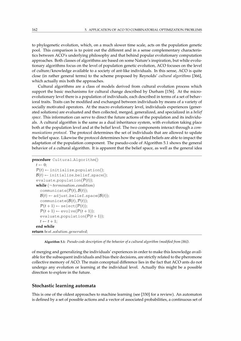
162 5. APPLICATION OF ACO TO COMBINATORIAL OPTIMIZATION PROBLEMS
to phylogenetic evolution, which, on a much slower time scale, acts on the population genetic
pool. This comparison is to point out the different and in a sense complementary characteris-
tics between ACO’s underlying philosophy and that behind popular evolutionary computation
approaches. Both classes of algorithms are based on some Nature’s inspiration, but while evolu-
tionary algorithms focus on the level of population genetic evolution, ACO focuses on the level
of culture/knowledge available to a society of ant-like individuals. In this sense, ACO is quite
close (in rather general terms) to the scheme proposed by Reynolds’ cultural algorithms [366],
which actually mix both the approaches.
Cultural algorithms are a class of models derived from cultural evolution process which
support the basic mechanisms for cultural change described by Durham [156]. At the micro-
evolutionary level there is a population of individuals, each described in terms of a set of behav-
ioral traits. Traits can be modified and exchanged between individuals by means of a variety of
socially motivated operators. At the macro evolutionary level, individuals experiences (gener-
ated solutions) are evaluated and then collected, merged, generalized, and specialized in a belief
space. This information can serve to direct the future actions of the population and its individu-
als. A cultural algorithm is the same as a dual inheritance system, with evolution taking place
both at the population level and at the belief level. The two components interact through a com-
munications protocol. The protocol determines the set of individuals that are allowed to update
the belief space. Likewise the protocol determines how the updated beliefs are able to impact the
adaptation of the population component. The pseudo-code of Algorithm 5.1 shows the general
behavior of a cultural algorithm. It is apparent that the belief space, as well as the general idea
procedure Cultural Algorithm()
t← 0;
P(t)← initialize population();
B(t)← initialize belief space();
evaluate population(P(t));
while (¬ termination condition)
communicate(P(t),B(t));
B(t)← adjust belief space(B(t));
communicate(B(t),P(t));
P(t+ 1)← select(P(t));
P(t+ 1)← evolve(P(t+ 1));
evaluate population(P(t+ 1));
t← t+ 1;
end while
return best solution generated;
Algorithm 5.1: Pseudo-code description of the behavior of a cultural algorithm (modified from [86]).
of merging and generalizing the individuals’ experiences in order to make this knowledge avail-
able for the subsequent individuals and bias their decisions, are strictly related to the pheromone
collective memory of ACO. The main conceptual difference lies in the fact that ACO ants do not
undergo any evolution or learning at the individual level. Actually this might be a possible
direction to explore in the future.
Stochastic learning automata
This is one of the oldest approaches to machine learning (see [330] for a review). An automaton
is defined by a set of possible actions and a vector of associated probabilities, a continuous set of
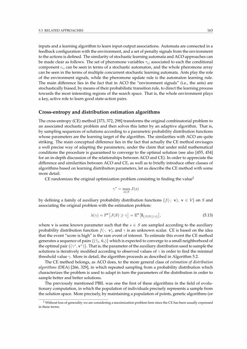
5.3 RELATED APPROACHES 163
inputs and a learning algorithm to learn input-output associations. Automata are connected in a
feedback configuration with the environment, and a set of penalty signals from the environment
to the actions is defined. The similarity of stochastic learning automata andACO approaches can
be made clear as follows. The set of pheromone variables τij associated to each the conditional
component ci, can be seen in terms of a stochastic automaton, and the whole pheromone array
can be seen in the terms of multiple concurrent stochastic learning automata. Ants play the role
of the environment signals, while the pheromone update rule is the automaton learning rule.
The main difference lies in the fact that in ACO the “environment signals” (i.e., the ants) are
stochastically biased, bymeans of their probabilistic transition rule, to direct the learning process
towards the most interesting regions of the search space. That is, the whole environment plays
a key, active role to learn good state-action pairs.
Cross-entropy and distribution estimation algorithms
The cross-entropy (CE) method [373, 372, 298] transforms the original combinatorial problem to
an associated stochastic problem and then solves this latter by an adaptive algorithm. That is,
by sampling sequences of solutions according to a parametric probability distribution functions
whose parameters are the learning target of the algorithm. The similarities with ACO are quite
striking. The main conceptual difference lies in the fact that actually the CE method envisages
a well precise way of adapting the parameters, under the claim that under mild mathematical
conditions the procedure is guaranteed to converge to the optimal solution (see also [455, 454]
for an in-depth discussion of the relationships between ACO and CE). In order to appreciate the
difference and similarities between ACO and CE, as well as to briefly introduce other classes of
algorithms based on learning distribution parameters, let us describe the CE method with some
more detail.
CE randomizes the original optimization problem consisting in finding the value2
γ∗ = maxs∈S
J(s)
by defining a family of auxiliary probability distribution functions f(·; v), v ∈ V on S and
associating the original problem with the estimation problem:
λ(γ) = Pv
[
J(S) ≥ γ]
= Ev
[
IJ(S)≥γ
]
, (5.13)
where v is some known parameter such that the s ∈ S are sampled according to the auxiliary
probability distribution function f(·; v), and γ is an unknown scalar. CE is based on the idea
that the event “score is high” is the rare event of interest. To estimate this event the CE method
generates a sequence of pairs (γt, vt)which is expected to converge to a small neighborhood of
the optimal pair (γ∗,v∗). That is, the parameter of the auxiliary distribution used to sample the
solutions is iteratively modified according to observed values of γ in order to find the minimal
threshold value γ. More in detail, the algorithm proceeds as described in Algorithm 5.2.
The CE method belongs, as ACO does, to the more general class of estimation of distribution
algorithms (DEA) [266, 329], in which repeated sampling from a probability distribution which
characterizes the problem is used to adapt in turn the parameters of the distribution in order to
sample better and better solutions.
The previously mentioned PBIL was one the first of these algorithms in the field of evolu-
tionary computation, in which the population of individuals precisely represents a sample from
the solution space. More precisely, by maintaining a population of points, genetic algorithms (or
2 Without loss of generality we are considering a maximization problem here since the CE has been usually expressedin these terms.
164 5. APPLICATION OF ACO TO COMBINATORIAL OPTIMIZATION PROBLEMS
1. Choose some v0, and set t = 1.
2. Generate a sample st = s1, . . . , sn according to the density f(·; vt−1).
3. Since γt is such that Pv
t−1[J(S) ≥ γt] ≥ ρ, the estimate γt of γt is computed as the desired
percentile of the sample: γt = (1− ρ)100%.
4. Use the same sample and the approximation γt of γt to solve the following stochastic prob-
lem:
vt = arg minv
Ev
t−1
[
IJ(S)≥γt log f(st; v)]
. (5.14)
5. Smooth out the value of vt as follows: vt = αvt + (1− α)vt−1.
6. If for some t ≥ d, where d is a small number (e.g., d = 5), γt = γt−1 = . . . = γt−d then stop,
otherwise reiterate from step 2.
Algorithm 5.2: Description of the general behavior of the cross-entropy method (modified from [298]).
similar evolutionary algorithms) can be viewed as creating implicit probabilistic models of the so-
lutions seen in the search. On the other hand, PBILwent precisely in the direction of maintaining
explicit and incremental information about which group of parameter values have contributed to
the generation of good quality solutions. Actually, even if derived in the context of genetic algo-
rithms, PBIL is more close to a cooperative system of stochastic learning automata in which the
automata choose their actions independently but all receive the same common reinforcement.
In this perspective, the difference with ACO can be appreciated even more according to the way
ACO has been related to stochastic learning automata. The basic ideas of PBIL have been further
enhanced in order to consider dependencies among the variables [12], in particular adding no-
tions and ideas from the domain of Bayesian networks, which are a popular and effective method
to model dependencies and independencies among random variables.
In general, a variety of methods have been proposed to effectively learn probability distri-
butions. ACO, CE, and PBIL being some of the most popular ones (see [266] for a review of
these methods in the specific field of evolutionary computation for continuous optimization).
The likely most critical aspects when these methods are applied to combinatorial problems con-
sists in the ability to take into account the tight relationships among the variables. In this sense
the ACO’s construction approach might be seen as an advantage over other methods working
directly in the solution space. The Blum’s thesis [44] contains insightful discussions about the
relationship between ACO and DEAs.
Neural networks
Ant colonies, being composed of numerous concurrently and locally interacting units, can be
seen as “connectionist” systems [165], the most famous examples of which are neural networks
[35, 223, 377]. From a structural point of view, the parallel between the ACO meta-heuristic and
a generic neural network can be drawn in the case of the original ACO definition by putting each
solution component ci in correspondence with a neuron νi, and the problem-specific neighbor-
hood of ci on the pheromone graph in correspondence with the set of synaptic-like links exiting
neuron νi, such that synapses are equivalent so the edges of the pheromone graph. The ants
themselves can be seen as input signals concurrently propagating through the neural network
and modifying the strength of the synaptic-like inter-neuron connections. Signals (ants) are lo-
cally propagated by means of a stochastic transfer function (the ant stochastic decision policy

5.3 RELATED APPROACHES 165
using only local information) and the more a synapse (a decision pair 〈ci|cj〉) is used, the more
the connection between its two end-neurons is reinforced. The ACO-synaptic learning rule can
be interpreted as an a posteriori rule: signals related to good examples, that is, ants which dis-
covered a good quality solution, reinforce the synaptic connections they traverse more than
signals related to poor examples.
The work of Chen [78], who proposed a neural network approach to TSP, bears important
similarities with the ACO approach. Like in ACO algorithms, a tour is built in an incremental
way, according to synaptic strengths. It makes also use of candidate lists and 2-opt local opti-
mization, similarly to ACS. The strengths of the synapses of the current tour and of all previous
tours are updated according to a Boltzmann-like rule and a learning rate playing the role of an
evaporation coefficient. Although there are some differences, the common features are, in this
case, striking.
Rollout algorithms
Rollout algorithms have been proposed by Bertsekas et al. [28] as a metaheuristic derived from
dynamic programming and that is expected to improve the effectiveness of a given heuristic
algorithm, which is rolled-out to obtain useful information to guide the construction of a solution
to the problem under consideration. The effectiveness of the approach, in the sense of improving
the quality of a given heuristic, is supported by the results of the application to a number of NP-
hard combinatorial optimization problems [25, 383, 209]. Moreover, the efficacy of the method
does not critically depend on any used-defined parameter, so that it is rather robust. The real
drawback of the algorithm consist in the fact that it is expected to be quite computationally
intensive.
The general rollout algorithm consists of a construction process that provides a solution to
the problem under investigation by starting with some partial solution x0 ∈ X and by including
a new component ci ∈ C at each step of the process. The different feasible options ck ∈ C(xj)available at the j-th step of the process are evaluated by using a base heuristicH in the following
way. It is assumed that, given a partial solution xj , H can determine from it a complete feasible
solution sj ∈ S, sj = H(xj), and a cost J(sj) can be assigned to it. Therefore, if xk+1 = xk ⊕ ckis the new partial solution that would be obtained by selecting ck as new component to include
into the partial solution xk, then, a complete feasible solution sk+1 is obtained by expanding
xk+1 through the heuristic H, sk+1 = H(xk+1), and the associated cost J(sk+1|ck) is calculatedand used as the cost to score the goodness of the choice ck. In practice, H provides a heuris-
tic completion of the current partial solution, and the final cost J is used as an evaluation of
cost-to-go associated to the choice ck. The alternative with the lowest cost-to-go, is chosen and
added to the partial solution, and the process is iterated. The algorithmic skeleton of the rollout
metaheuristic is reported in the pseudo-code of the Algorithm box 5.3.
The relationship with dynamic programming is apparent from both the construction ap-
proach and the fact that each choice is scored according to an estimate of the cost-to-go asso-
ciated to that choice. The truly innovative component of rollout algorithms consists in the use of
a heuristic to provide an approximate evaluation of the cost, instead of relying on the systematic
expansion of all the possible completions from the current partial solution. This is equivalent
to the use of approximate cost-to-go functions mentioned in Subsection 3.4.3. However, in this
case, the approximation function is a heuristic algorithm, and not, for instance a neural network.
A more general possibility consists in using a pool of heuristics, which are weighted with some
scalar weights in order to provide a better approximation. More in general, a variety of alter-
native schemes can be adopted (see the original paper [28]), and for some of them it can be
guaranteed that the rollout algorithm will outperform the base heuristic algorithm H. In inter-
esting way of choosing the heuristicH is like in [209], in whichH is composed of two parts: one
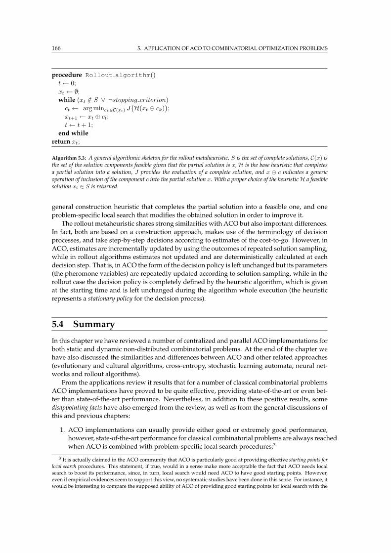
166 5. APPLICATION OF ACO TO COMBINATORIAL OPTIMIZATION PROBLEMS
procedure Rollout algorithm()
t← 0;
xt ← ∅;while (xt /∈ S ∨ ¬stopping criterion)
ct ← arg minck∈C(xt) J(
H(xt ⊕ ck))
;
xt+1 ← xt ⊕ ct;t← t+ 1;
end while
return xt;
Algorithm 5.3: A general algorithmic skeleton for the rollout metaheuristic. S is the set of complete solutions, C(x) isthe set of the solution components feasible given that the partial solution is x, H is the base heuristic that completesa partial solution into a solution, J provides the evaluation of a complete solution, and x ⊕ c indicates a genericoperation of inclusion of the component c into the partial solution x. With a proper choice of the heuristicH a feasiblesolution xt ∈ S is returned.
general construction heuristic that completes the partial solution into a feasible one, and one
problem-specific local search that modifies the obtained solution in order to improve it.
The rollout metaheuristic shares strong similarities with ACO but also important differences.
In fact, both are based on a construction approach, makes use of the terminology of decision
processes, and take step-by-step decisions according to estimates of the cost-to-go. However, in
ACO, estimates are incrementally updated by using the outcomes of repeated solution sampling,
while in rollout algorithms estimates not updated and are deterministically calculated at each
decision step. That is, in ACO the form of the decision policy is left unchanged but its parameters
(the pheromone variables) are repeatedly updated according to solution sampling, while in the
rollout case the decision policy is completely defined by the heuristic algorithm, which is given
at the starting time and is left unchanged during the algorithm whole execution (the heuristic
represents a stationary policy for the decision process).
5.4 Summary
In this chapter we have reviewed a number of centralized and parallel ACO implementations for
both static and dynamic non-distributed combinatorial problems. At the end of the chapter we
have also discussed the similarities and differences between ACO and other related approaches
(evolutionary and cultural algorithms, cross-entropy, stochastic learning automata, neural net-
works and rollout algorithms).
From the applications review it results that for a number of classical combinatorial problems
ACO implementations have proved to be quite effective, providing state-of-the-art or even bet-
ter than state-of-the-art performance. Nevertheless, in addition to these positive results, some
disappointing facts have also emerged from the review, as well as from the general discussions of
this and previous chapters:
1. ACO implementations can usually provide either good or extremely good performance,
however, state-of-the-art performance for classical combinatorial problems are always reached
when ACO is combined with problem-specific local search procedures;3
3 It is actually claimed in the ACO community that ACO is particularly good at providing effective starting points forlocal search procedures. This statement, if true, would in a sense make more acceptable the fact that ACO needs localsearch to boost its performance, since, in turn, local search would need ACO to have good starting points. However,even if empirical evidences seem to support this view, no systematic studies have been done in this sense. For instance, itwould be interesting to compare the supposed ability of ACO of providing good starting points for local search with the
5.4 SUMMARY 167
2. when compared to related exact methods like dynamic programming, it becomes ap-
parent that only a small fraction of state information is usually retained in the adopted
pheromone models, such that the associated loss of fundamental information determines
that only asymptotic guarantees of convergence can be given (under mild assumptions),
while finite-time performance critically depends on how the design choices (e.g., the cho-
sen pheromone model) accounts for the specific problem characteristics, and in general no
guarantees can be given;
3. the potentialities of the multi-agent and distributed ACO’s architecture, directly stem-
ming from the biological context of inspiration, are not really exploited in the case of non-
distributed problems;4
4. even if ACO was one of the first frameworks based on the use of learning strategies to
attack hard combinatorial problems several other similar and equally good approaches
exist (e.g., distribution estimation algorithms, cross entropy, cultural algorithms), such that
ACO cannot be really seen anymore as a particularly innovative approach for the field.
On the other hand, the application of ACO to problems of adaptive routing in telecommuni-
cation networks is equally successful (see following Chapters 7 and 8) than the application to
classical non-distributed combinatorial problems, but at the same time does not suffer from the
“drawbacks” (1-4) and enjoys some additional appealing properties. Let us discuss these facts
with some detail.
The problem of routing in telecommunication networks is the problem of finding the joint
set of paths connecting traffic sources to traffic destinations that minimize some network-wide
cost criteria. In the general and most common cases, the precise properties of the processes reg-
ulating the arrivals and the characteristics of the traffic sessions are unknown a priori, and the
overall solution to the problem, in terms of setting a routing policy at the nodes, is expected to
continually adapt to the ever changing traffic patterns and must be provided online in a fully
decentralized and distributed way. It is apparent that all these characteristics closely match
those of ACO and of its biological context of inspiration in terms of fully distributed environ-
ment, stigmergic communication, concurrent search for minimum cost paths, adaptation over
time, etc. This results in the fact that the application of ACO to routing, or, more in general,
to control problems in telecommunication networks, is at the same time extremely natural and
also successful. While in the case of classical combinatorial problem the choice of an effective
pheromone model is one of the main issues that the algorithm designer has to deal with, in the case
of routing in networks the choice for the pheromone model is naturally dictated by the intrin-
sic characteristics of the problem: the network nodes ck, k = 1, . . . , N are the decisions points
(i.e., the solution components) holding the pheromone tables T ck , and each pheromone variable
τ ck
nd represents, for each locally known final destination d, d 6= ck, d ∈ 1, . . . , N, and for each
one of the feasible next hop nodes n ∈ N (ck) (e.g., the nodes in the radio range or those di-
rectly connected by cables), the locally estimated goodness of forwarding a data packet through
the neighbor n when its final destination is d. It is not by chance that all the instances of ACO
algorithms for routing follow this general scheme for their pheromone model.5
STAGE algorithm of Boyan and Moore [55] which makes use of value functions to learn precisely good starting pointsfor local search by exploiting the same trajectories generated by repeated runs of local search.
4 It is usually true that for a statically defined and centralized problem a monolithic approach is the most efficientone from a computational point of view.
5 Clearly, if even if the structure of the pheromonemodel is naturally mapped onto the network structure, there is stillthe problem of defining what the pheromone precisely represents (e.g., the expected end-to-end delay, the remainingnumber of hops, etc.) and how to evaluate a path given the non-stationarity of the traffic conditions. Different ACOalgorithms for routing have implemented different ways of dealing with these problems. These issues will be discussedin depth when AntNet will be introduced in Chapter 7.
168 5. APPLICATION OF ACO TO COMBINATORIAL OPTIMIZATION PROBLEMS
Given this distributed organization of the pheromone tables, the ACO’s ants become true
mobile stigmergic agents, sampling paths between source-destination nodes and repeatedly and
concurrently updating the pheromone (routing) tables at the nodes in order to adapt the overall
control policy to the changing traffic conditions. While in the static and non-distributed case
the multi-agent architecture of ACO was more an abstraction than a real issue, in the case of
network problems it becomes necessary to think of the ants are actual mobile agents (or routing
packets) physically moving from one node to an adjacent one.
Moreover, in network environments the notion of local search becomes rather meaningless,
such that state-of-the-art performance can be and are obtained by genuine ACO implementa-
tions, without the need of daemon components to boost up the performance.
Also the issue of convergence becomes of less practical importance than in the static case,
due to the fact that in dynamic environments rather than convergence in (unlikely) situations
of stationarity, it is more important the ability of the algorithm to effectively adapt to the ever
changing situations without incurring in counterproductive oscillations or delays. And this is
what ACO ants can effectively do by repeated Monte Carlo sampling of paths and updating of
the pheromone tables.
Finally, ACO’s ideas, once translated into a routing algorithm almost naturally result in a de-
sign made of several components (active information gathering by using mobile agents, stochas-
tic decisions, Monte-Carlo-based adaptive learning, availability of multiple paths, robustness to
agent failures) that make the ACO-based approach as a truly innovative one in the domain of routing
and, more in general, of control algorithms for telecommunication networks. Going further, we
conjecture that ACO-based approaches have good chances of increasing their popularity over
the years with the increase of the number of different services offered by the networks and the
evolution of network architectures in the direction of becoming more and more active [420] and
heterogeneous.
REMARK 5.1 (The choice of focusing on the application of ACO to network problems): All these
facts seem to suggest that the application of ACO to adaptive problems in telecommunication networks is
at the same time more natural, sound, innovative, closer to the original biological framework of inspiration,
and open to future developments than the application to classical non-distributed combinatorial problems.
Therefore, we are going to focus exclusively on the application of ACO to telecommunication networks in
the second part of the thesis, starting from the next chapter.
Part II
Application of ACO to problems of
adaptive routing in
telecommunication networks

CHAPTER 6
Routing in telecommunication
networks
This second part of the thesis is devoted to the description and discussion of a family of ACO al-
gorithms for adaptive multipath routing in telecommunication networks. Therefore, this first chapter
provides the generalities on the problem of routing in telecommunication networks and dis-
cusses the salient characteristics of some of the most popular routing schemes. In particular, we
discuss the characteristics of adaptive and multipath routing solutions versus static and single-
path strategies. Moreover, according to the fact that most of the experimental results that will
be presented in the following chapters concern wired IP wide-area networks, the discussions of
this chapter mainly focus on this specific but extremely important class of networks.
One of the aims of the chapter is to show that there are still several important open issues and
quite unexplored directions in the domain of routing algorithms. In particular, true adaptivity
to changing traffic patterns is still far from being reached and very few algorithms make use of
multiple paths. Most of the focus in the routing community has been so far on overall robustness,
adaptivity to topological changes and single shortest path solutions. Also, strategies based on
stochastic decisions and active information gathering bymeans ofmobile agents have not gained
so far much popularity. On the other hand, adaptivity, discovery and use of multiple paths,
use of stochastic components, and repeated path sampling and updating are at the very core
of the design of the ACO algorithms for routing that will be introduced in the next chapter.
Therefore, in the following of this chapter we discuss these specific issues in relationship to the
characteristics of the most widely in use and consolidated routing algorithms.
The chapter can be also considered as a high-level overview on routing algorithms. Its con-
tent is complemented by that of Appendix F, which provides a general overview on telecommu-
nication networks, their architectures, transmission technologies, forwarding mechanisms, and
so on.
Organization of the chapter
Section 6.1 introduces the general characteristics of routing and of generic routing strategies.
Section 6.2 and its subsections provide a classification of routing algorithms based on: the con-
trol architecture (Subsection 6.2.1), the way, static or adaptive, routing tables are set up (Subsec-
tion 6.2.2), the general characteristics of the solution strategy, which can be in general based on
optimal or shortest path routing (Subsection 6.2.3), and the strategies to forward data, that can
make use of a single or multiple paths at the same time (Subsection 6.2.4). Section 6.3 considers
the most used metrics for network performance evaluation, while Section 6.4 and its subsec-
tions are devoted to discuss the characteristics and the relationships of optimal and shortest
path routing. Optimal routing is described in Subsection 6.4.1, while the two most in use classes
of shortest path algorithms, that is, distance-vector and link-state algorithms, are discussed re-
spectively in Subsection 6.4.2.1, and Subsection 6.4.2.2. Subsection 6.4.3 succinctly discusses the

172 6. ROUTING IN TELECOMMUNICATION NETWORKS
relationships between optimal and shortest path routing, both from the perspective of game
theory, in terms of cooperative vs. non-cooperative games, and of the inverse problem of trans-
forming a shortest path problem into an optimal routing one. The section is concluded by an
historical glance at the routing on the Internet, provided in Section 6.5. The chapter’s Summary
summarizes all themajor characteristics of the discussed algorithms, points out their drawbacks,
and compiles a sort of wish list of properties that novel and innovative routing algorithms are
expected to show. ACO algorithms are precisely designed after these properties.
6.1 Routing: Definition and characteristics
Routing is at the core of any network control system, strongly affecting the overall network per-
formance.1 Routing can be characterized in the following general way. Let the network be
represented in terms of a directed weighted graph G = (V,E), where each node in the set V
represents a processing and forwarding unit and each edge in E is a transmission system with some
capacity/bandwidth and propagation characteristics. Data traffic originates from one node (end-
point) and can be directed to another node (unicast traffic), to a set of other nodes (multicast traffic)
and/or to all the other nodes (broadcast traffic). The node from where the traffic flow originates
is also called source, or starting end-point, while the nodes to which traffic is directed are the
final end-points, or destinations. The nodes in-between that forward traffic from sources to des-
tinations are called intermediate, or relay, nodes. A flow is a vector in R|E| that for a traffic pair
(s,D), s ∈ V,D ⊆ V , assigns a way of forwarding the data traffic from s to the nodes in D
across the network while respecting the edge capacities and such that the sum of entering flows
minus exiting flows at each node is null (more in general, a flow can be considered in the terms
of defining a forwarding (multi-)path across the network for a traffic session, and such that both
temporary data buffering and data losses can happen).
DEFINITION 6.1 (Routing problem): The general routing problem is the problem of defining path flows
to forward incoming data traffic such that the overall network performance is maximized. At each node
data is forwarded according to a decision policy parametrized by a local data structure called routing
table. In this sense, a routing system can be properly seen as a distributed decision system.
According to the different characteristics of the processing and transmission components, as
well as of traffic pattern and type of performance expected to be delivered (see Appendix F for a
discussion on network classifications), a variety of different classes of specific routing problems
of practical and theoretical interest can be defined. For example, routing telephone calls in a
network of mobile devices is a problem presenting characteristics which are quite different from
those of the problem of routing telephone calls in a cable telephone network, which, in turn, is a
problemmuch different from the problem of routing data packets in a best-effort connection-less
data network as the Internet.
An important difference between routing and the combinatorial problems that have been
considered so far consists in the presence of input data traffic which characterizes the problem
instance. That is, the routing problem is composed of two parts: (i) the communication struc-
ture, which in a sense defines the constraints, and (ii) the traffic patterns that make use of this
structure. It is always necessary to reason taking into account the two aspects together. For
instance, the set of all the disjoint shortest paths (taken with respect to link bandwidths and
1 A network control architecture is the set of protocols, policies and algorithms used to control a (partition of a)network. Therefore, usually routing participate to the control together with a number of other additional components,like the congestion control one (e.g., TCP on the Internet) or the admission control one (e.g., call admission in telephonenetworks).
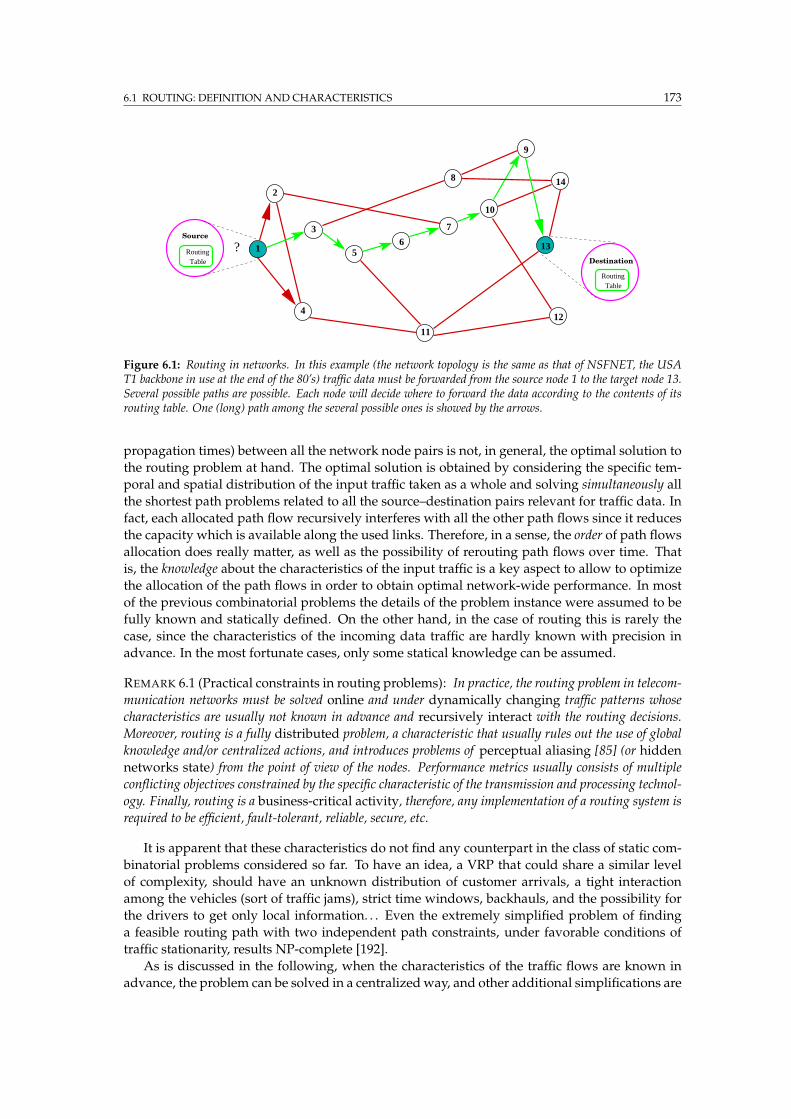
6.1 ROUTING: DEFINITION AND CHARACTERISTICS 173
1
3
4
5
7
8
9
14
11
12
RoutingTable
Source
?
RoutingTable
6
10
13
2
Destination
Figure 6.1: Routing in networks. In this example (the network topology is the same as that of NSFNET, the USAT1 backbone in use at the end of the 80’s) traffic data must be forwarded from the source node 1 to the target node 13.Several possible paths are possible. Each node will decide where to forward the data according to the contents of itsrouting table. One (long) path among the several possible ones is showed by the arrows.
propagation times) between all the network node pairs is not, in general, the optimal solution to
the routing problem at hand. The optimal solution is obtained by considering the specific tem-
poral and spatial distribution of the input traffic taken as a whole and solving simultaneously all
the shortest path problems related to all the source–destination pairs relevant for traffic data. In
fact, each allocated path flow recursively interferes with all the other path flows since it reduces
the capacity which is available along the used links. Therefore, in a sense, the order of path flows
allocation does really matter, as well as the possibility of rerouting path flows over time. That
is, the knowledge about the characteristics of the input traffic is a key aspect to allow to optimize
the allocation of the path flows in order to obtain optimal network-wide performance. In most
of the previous combinatorial problems the details of the problem instance were assumed to be
fully known and statically defined. On the other hand, in the case of routing this is rarely the
case, since the characteristics of the incoming data traffic are hardly known with precision in
advance. In the most fortunate cases, only some statical knowledge can be assumed.
REMARK 6.1 (Practical constraints in routing problems): In practice, the routing problem in telecom-
munication networks must be solved online and under dynamically changing traffic patterns whose
characteristics are usually not known in advance and recursively interact with the routing decisions.
Moreover, routing is a fully distributed problem, a characteristic that usually rules out the use of global
knowledge and/or centralized actions, and introduces problems of perceptual aliasing [85] (or hidden
networks state) from the point of view of the nodes. Performance metrics usually consists of multiple
conflicting objectives constrained by the specific characteristic of the transmission and processing technol-
ogy. Finally, routing is a business-critical activity, therefore, any implementation of a routing system is
required to be efficient, fault-tolerant, reliable, secure, etc.
It is apparent that these characteristics do not find any counterpart in the class of static com-
binatorial problems considered so far. To have an idea, a VRP that could share a similar level
of complexity, should have an unknown distribution of customer arrivals, a tight interaction
among the vehicles (sort of traffic jams), strict time windows, backhauls, and the possibility for
the drivers to get only local information. . . Even the extremely simplified problem of finding
a feasible routing path with two independent path constraints, under favorable conditions of
traffic stationarity, results NP-complete [192].
As is discussed in the following, when the characteristics of the traffic flows are known in
advance, the problem can be solved in a centralized way, and other additional simplifications are
174 6. ROUTING IN TELECOMMUNICATION NETWORKS
possible, routing can be framed in the general terms of a multi-commodity flow problem (e.g., [24,
344]), which is an important class of problemsmodeling the transfer of commodities from source
locations to destinations.
There is an extensive literature concerning routing issues, and, more in general, network
communications systems. This material is not duplicated here. This chapter contains only a
short and necessarily incomplete overview on the main characteristics of network systems and
on routing in particular, focusing on those aspects that are of specific interest for the ACO algo-
rithms presented in the following. For more general and comprehensive treatments, the reader
is referred, for example, to [26, 419, 398, 439]. In particular, the Bertsekas and Gallager [26]
and Tanenbaum’s [419] textbooks contain comprehensive and accurate treatments of most of the
general issues concerning the characteristics, design and control of data networks. For more
specific reviews, the reader is referred for example to [359, 61] for routing techniques in mo-
bile networks, to [79, 208, 81] for issues concerning routing in high-speed networks providing
Quality-of-Service (QoS), and to [217, 398] for routing on the Internet.
In spite of the aspects that characterize each specific routing problem at hand, any routing
strategy virtually consists of the same set of activities carried out at each node, as shown in
Algorithm 6.1, which can be seen as a sort of generalmeta-algorithm for routing. Clearly, different
strategies implement each of the operations of the meta-algorithm in a possibly different way
according to the specificities of the problem and of the design choices.
At each network node:
1. Acquisition and organization of up-to-date information concerning the local state, that is,
information on the local traffic flows and on the status of the locally available resources;
2. Build up a view of the global network state, possibly by some form of exchanging of the local
state information;
3. Use of the global view to set up the values of the local routing table and, consequently, to
define the local routing policywith the perspective of optimizing some measure of network
performance;
4. Forward of the user traffic according to the defined routing policy.
5. Asynchronously and concurrently with the other nodes repeat the previous activities over
time.
Algorithm 6.1: Meta-algorithm for routing, describing the general activities concurrently carried out at each node inorder to realize the network-wide routing function.
6.2 Classification of routing algorithms
Routing algorithms are usually designed in relationship to the type of both the network and the
services delivered by the network. Under this perspective, given the variety of possible network
types and delivered services as briefly discussed in Appendix F, it is hard to identify meaningful
and exhaustive classifications for routing algorithms. Therefore, in the following the algorithms
are classified according to few very general characteristics that can be singled out. In particu-
lar, Subsection 6.2.1 discusses the differences between algorithms using a centralized control and
those using a distributed control (in the following only distributed algorithms are considered).
Additional general characteristics that can be used to classify routing algorithms can be derived
6.2 CLASSIFICATION OF ROUTING ALGORITHMS 175
by the meta-algorithm, which suggests that different choices for either the optimization criteria
or the strategies for building and using the local and the global views can result in different
classes of algorithms. In particular, since the strategies for building the local and global views
are strictly related to the way both traffic information and topological information are managed in
order to define the routing tables, a classification of the different routing systems is precisely
given according to the algorithm behavior, which can be static or adaptive with respect to topol-
ogy and/or traffic patterns. Moreover, since different choices in the criterion to be optimized
can generate different classes of algorithms, a further classification is given in this sense, making
a distinction between optimal and shortest path routing. A final classification is drawn according
to the number of paths that are used or maintained for the same traffic session or destination. In
this sense, algorithms are divided in single-path, multi-path and alternate-path.
6.2.1 Control architecture: centralized vs. distributed
In centralized algorithms, a main controller is responsible for the updating of all the node routing
tables and/or for every routing decision. Centralized algorithms can be used only in particular
cases and for small networks. In general, the controller has to gather information about the
global network status and has to transmit all the decisions/updates. The relatively long time
delays necessarily involved with such activities, as well as the lack of fault-tolerance (if not at
the expenses of redundant duplications), make centralized approaches unfeasible in practice.
From now on only non-centralized, that is, distributed routing systems are considered.
In distributed routing systems, every node autonomously decide about local data forwarding.
At each node a local routing table is maintained in order to implement the local routing policy.
The distributed paradigm is currently used in the majority of network systems.
6.2.2 Routing tables: static vs. dynamic
Routing tables can be statically assigned or dynamically built and updated. It is evident that the
performance of the two approaches can be radically different, and the appropriateness of one
approach over the other tightly depends on the characteristics of the network scenario under
consideration.
In both cases routing tables are built in order to possibly optimize some network-wide criteria
which are made depending in turn on costs associated to network elements. That is, to each link,
or whatever network resource of interest (e.g., available processing power of a routing node),
a value (integer, real, nominal, etc.), here called cost, is assigned according to some metric in
order to have a measure of either utilization level or physical characteristics (e.g., bandwidth,
propagation delay). Therefore, the process of finding routing paths optimizedwith respect to the
chosen criteria can be actually intended as the minimization process with respect to the defined
costs (e.g, the overall cost criterion can be expressed in in terms of a sum of the link costs or of
the path/link flows). If trusting information about the incoming traffic patterns is available, then
an optimal routing approach (i.e., a multi-commodity flow formulation) can be used to actually
carry the minimization, otherwise other approaches, like those based on independent shortest
path calculations, are called for.
Static routing
In static (or oblivious) routing systems, the path to forward traffic between pairs of nodes is de-
termined without regard to the current network state. The paths are usually chosen as the result
of the offline optimization of some selected cost criterion. Once defined the paths to be used for
each source-destination pair, data are always forwarded along these paths.
176 6. ROUTING IN TELECOMMUNICATION NETWORKS
Costs, and, accordingly, routing tables, are assigned either by an operator or through auto-
matic procedures independently from the current traffic events. The use of the links’ physical
characteristics is one of the simplest ways to assign static link costs (e.g., a link with characteris-
tics of high bandwidth and low propagation delay will have associated a low cost). For instance,
the cost default value of a link for the Internet intra-domain protocol Open Shortest Path First
(OSPF) [328, 326] as automatically assigned by most CISCO routers is 108/b, with b being the
unload bandwidth of the link [332].
Routing tables can be also assigned on the basis of some a priori knowledge about the ex-
pected input traffic. For instance, traffic statistics can be periodically recorded, and if some
regularities can be spot, these can be used in turn to model the incoming traffic and assign the
routing tables as the result of optimal routing calculations.
Dynamic routing
Dynamic (or adaptive) routing goes beyond static routing by admitting the possibility of build-
ing/changing the routing tables online according to the current traffic events. It is useful to
distinguish between the ability of adapting to the changing traffic conditions and to topological
modifications (e.g., link/node failures, link/node addition/removal).
Topological adaptivity is in a sense more fundamental. It is not reasonable to think that every
resource addition/removal should be explicitly notified by the human operator. Instead, is a
minimal requirement to ask the distributed routing system to have the ability to automatically
get aware of such modifications. This is what actually happens in most of the currently used
routing protocols. Clearly, different protocols react in different way to such events. For instance,
classical Bellman-Ford algorithms (see in the following), since they do not make explicit use of
global network topology and only use the notion of distance, suffer the problem of the so-called
counting-to-infinity [26], that is, when a link becomes suddenly unavailable, in the worst case it
might take infinite time to adjust the routing tables accordingly.
On the other hand, the most common intra-domain routing protocol, OSPF [328], is a shortest
path algorithm based on topology broadcast and is able to be fully and efficiently adaptive with
respect to topological modifications. However, OSPF is not really adaptive with respect to traffic
modifications, such that link costs are static, and may change only when network components
become unreachable or new ones come up.
As another example, the Enhanced Interior Gateway Routing Protocol (EIGRP), which is the
CISCO’s proprietary intra-domain protocol, is an extension of the Bellman-Ford based on the
DUAL algorithm [189], such that it overcomes the counting-to-infinity problem and uses link
costs which are dynamically assigned according to the following formula:
C =
[
k1B +k2B
256− L + k3D
]
k5
R− k4, (6.1)
where ki, i = 1, . . . , 5 are constants, L is the link load assigned as an integer over a scale going
from 1 to 255,D is the topological delay, that is, the amount of time it takes to get to the destina-
tion using that link in case of unloaded network, R is the reliability of the path expressed as the
fraction of packets that will arrive at destination undamaged, and B =107
mini bi, where bi is the
bandwidth of the path to destination. The parameters B and D are defined during the router
configuration, while L and R are estimated through measurements. However, the default link
cost is also defined as C = B +D.
Generally speaking, adaptiveness to traffic events is commonly obtained by monitoring local
resource utilization (usually in terms of link costs), building up statical estimates of these costs,
using these costs to update the local routing table and possibly exchanging this information with
6.2 CLASSIFICATION OF ROUTING ALGORITHMS 177
other nodes in order to allow some form of dissemination of fresh local information. The nature
of the local statistical information, and the modalities of information exchange characterize the
different algorithms.
Adaptive routers are, in principle, the most attractive ones, because they can adapt the rout-
ing policy to varying traffic conditions. As a drawback, they can cause oscillations and incon-
sistencies in the selected paths, and, in turn, these can cause, circular paths, as well as large
fluctuations in measured performance. Stability and inconsistency problems are more evident
for connection-less than for connection-oriented networks [26] (see Appendix F for network clas-
sifications). The problems with adaptive routing are well captured by the following sentence,
slightly changed from the original citation: Link arrival rates depend on routing, which in turn de-
pends on arrival rates via routing selected paths, with a feedback effect resulting [26, Page 412].
Intuitively, the general non stationarity of the traffic patterns, as well as the above feedback
effect, generate non-trivial problems of parameters setting in any adaptive algorithm. If the
link costs are adaptively assigned in function of the locally observed traffic flows, which is, for
instance, the amount of the variation in the traffic flows that should trigger an update of the
link costs and in turn of the routing table? Should every update trigger a transmission of the
new costs / routing table to other nodes in the network? In general, every answer to these
questions will contain some level of arbitrariness. In fact, the values assigned to the parameters
of the algorithm define the tradeoff between reactivity to local traffic changes and stability in the
overall network response.
6.2.3 Optimization criteria: optimal vs. shortest paths
Shortest path routing [26, 441, 398] is the routing paradigm most in use in real networks. In short-
est path routing the optimizing strategy for path flows consists in using the minimum cost paths
connecting all the node pairs in the network, where the paths are calculated independently for
each pair. That is, shortest path routing adopts a per pair perspective. On the other hand, op-
timal routing [26], which is the other main reference paradigm (at least from a theoretical point
of view), has a network-wide perspective, since the path flows are calculated considering all
the incoming traffic sessions. Clearly, in order to adopt such a global strategy, optimal routing
requires the prior knowledge of the statistical characteristics of all the incoming flows, a require-
ment which is usually quite hard to satisfy.
Considered the importance, both theoretical and practical, of optimal and shortest path rout-
ing, Section 6.4 and its subsections are completely devoted to a detailed description and discus-
sion of these two approaches.
According to an optimization perspective, a more coarse-grained distinction can be also
made between minimal and non-minimal routing algorithms. Minimal routers allow packets to
choose only paths which are minimal with respect to some cost criterion, while in non-minimal
algorithms packets can be forwarded along any of the available paths according to some heuris-
tic decision strategy [45]. Both optimal and pure shortest path routing implement minimal
routers. On the other hand, ACO algorithms for routing are not minimal, due to the presence of
stochastic components playing a major role in decision-taking.
6.2.4 Load distribution: single vs. multiple paths
Data traffic toward the same destination d can be forwarded along always the same link or it
can be spread along multiple paths.2 Actually, when routing tables are updated being adaptive
to traffic patterns, the resulting effect can be that of actually spreading the data packets toward
2 In the following of this section the term “path” if often used instead of “link”, to actually indicate the path todestination which is associated to a specific local link. Links and paths plays essentially the same role in connection-
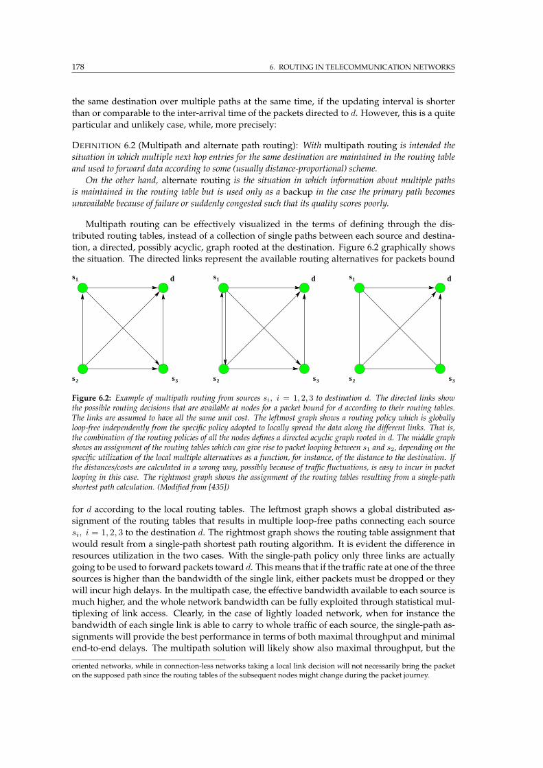
178 6. ROUTING IN TELECOMMUNICATION NETWORKS
the same destination over multiple paths at the same time, if the updating interval is shorter
than or comparable to the inter-arrival time of the packets directed to d. However, this is a quite
particular and unlikely case, while, more precisely:
DEFINITION 6.2 (Multipath and alternate path routing): With multipath routing is intended the
situation in which multiple next hop entries for the same destination are maintained in the routing table
and used to forward data according to some (usually distance-proportional) scheme.
On the other hand, alternate routing is the situation in which information about multiple paths
is maintained in the routing table but is used only as a backup in the case the primary path becomes
unavailable because of failure or suddenly congested such that its quality scores poorly.
Multipath routing can be effectively visualized in the terms of defining through the dis-
tributed routing tables, instead of a collection of single paths between each source and destina-
tion, a directed, possibly acyclic, graph rooted at the destination. Figure 6.2 graphically shows
the situation. The directed links represent the available routing alternatives for packets bound
d
ss
s1
2 3
d
ss
s1
2 3
d
ss
s1
2 3
Figure 6.2: Example of multipath routing from sources si, i = 1, 2, 3 to destination d. The directed links showthe possible routing decisions that are available at nodes for a packet bound for d according to their routing tables.The links are assumed to have all the same unit cost. The leftmost graph shows a routing policy which is globallyloop-free independently from the specific policy adopted to locally spread the data along the different links. That is,the combination of the routing policies of all the nodes defines a directed acyclic graph rooted in d. The middle graphshows an assignment of the routing tables which can give rise to packet looping between s1 and s2, depending on thespecific utilization of the local multiple alternatives as a function, for instance, of the distance to the destination. Ifthe distances/costs are calculated in a wrong way, possibly because of traffic fluctuations, is easy to incur in packetlooping in this case. The rightmost graph shows the assignment of the routing tables resulting from a single-pathshortest path calculation. (Modified from [435])
for d according to the local routing tables. The leftmost graph shows a global distributed as-
signment of the routing tables that results in multiple loop-free paths connecting each source
si, i = 1, 2, 3 to the destination d. The rightmost graph shows the routing table assignment that
would result from a single-path shortest path routing algorithm. It is evident the difference in
resources utilization in the two cases. With the single-path policy only three links are actually
going to be used to forward packets toward d. This means that if the traffic rate at one of the three
sources is higher than the bandwidth of the single link, either packets must be dropped or they
will incur high delays. In the multipath case, the effective bandwidth available to each source is
much higher, and the whole network bandwidth can be fully exploited through statistical mul-
tiplexing of link access. Clearly, in the case of lightly loaded network, when for instance the
bandwidth of each single link is able to carry to whole traffic of each source, the single-path as-
signments will provide the best performance in terms of both maximal throughput and minimal
end-to-end delays. The multipath solution will likely show also maximal throughput, but the
oriented networks, while in connection-less networks taking a local link decision will not necessarily bring the packeton the supposed path since the routing tables of the subsequent nodes might change during the packet journey.
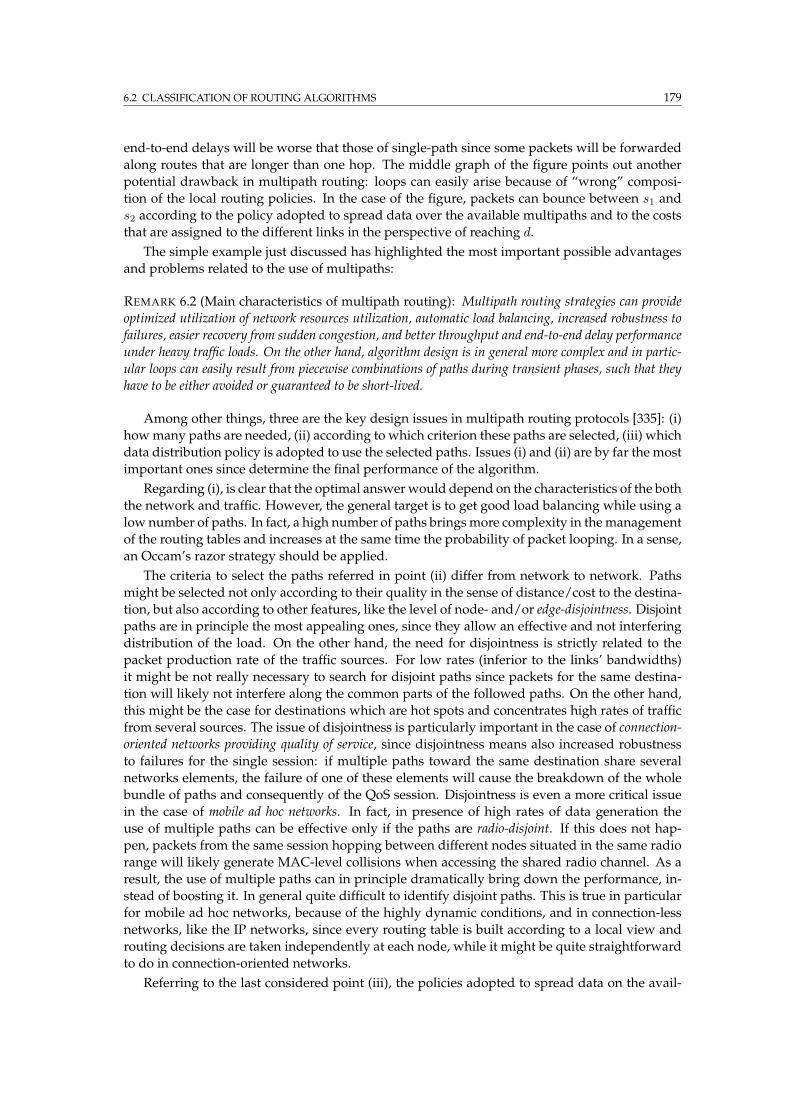
6.2 CLASSIFICATION OF ROUTING ALGORITHMS 179
end-to-end delays will be worse that those of single-path since some packets will be forwarded
along routes that are longer than one hop. The middle graph of the figure points out another
potential drawback in multipath routing: loops can easily arise because of “wrong” composi-
tion of the local routing policies. In the case of the figure, packets can bounce between s1 and
s2 according to the policy adopted to spread data over the available multipaths and to the costs
that are assigned to the different links in the perspective of reaching d.
The simple example just discussed has highlighted the most important possible advantages
and problems related to the use of multipaths:
REMARK 6.2 (Main characteristics of multipath routing): Multipath routing strategies can provide
optimized utilization of network resources utilization, automatic load balancing, increased robustness to
failures, easier recovery from sudden congestion, and better throughput and end-to-end delay performance
under heavy traffic loads. On the other hand, algorithm design is in general more complex and in partic-
ular loops can easily result from piecewise combinations of paths during transient phases, such that they
have to be either avoided or guaranteed to be short-lived.
Among other things, three are the key design issues in multipath routing protocols [335]: (i)
howmany paths are needed, (ii) according to which criterion these paths are selected, (iii) which
data distribution policy is adopted to use the selected paths. Issues (i) and (ii) are by far the most
important ones since determine the final performance of the algorithm.
Regarding (i), is clear that the optimal answerwould depend on the characteristics of the both
the network and traffic. However, the general target is to get good load balancing while using a
low number of paths. In fact, a high number of paths bringsmore complexity in themanagement
of the routing tables and increases at the same time the probability of packet looping. In a sense,
an Occam’s razor strategy should be applied.
The criteria to select the paths referred in point (ii) differ from network to network. Paths
might be selected not only according to their quality in the sense of distance/cost to the destina-
tion, but also according to other features, like the level of node- and/or edge-disjointness. Disjoint
paths are in principle the most appealing ones, since they allow an effective and not interfering
distribution of the load. On the other hand, the need for disjointness is strictly related to the
packet production rate of the traffic sources. For low rates (inferior to the links’ bandwidths)
it might be not really necessary to search for disjoint paths since packets for the same destina-
tion will likely not interfere along the common parts of the followed paths. On the other hand,
this might be the case for destinations which are hot spots and concentrates high rates of traffic
from several sources. The issue of disjointness is particularly important in the case of connection-
oriented networks providing quality of service, since disjointness means also increased robustness
to failures for the single session: if multiple paths toward the same destination share several
networks elements, the failure of one of these elements will cause the breakdown of the whole
bundle of paths and consequently of the QoS session. Disjointness is even a more critical issue
in the case of mobile ad hoc networks. In fact, in presence of high rates of data generation the
use of multiple paths can be effective only if the paths are radio-disjoint. If this does not hap-
pen, packets from the same session hopping between different nodes situated in the same radio
range will likely generate MAC-level collisions when accessing the shared radio channel. As a
result, the use of multiple paths can in principle dramatically bring down the performance, in-
stead of boosting it. In general quite difficult to identify disjoint paths. This is true in particular
for mobile ad hoc networks, because of the highly dynamic conditions, and in connection-less
networks, like the IP networks, since every routing table is built according to a local view and
routing decisions are taken independently at each node, while it might be quite straightforward
to do in connection-oriented networks.
Referring to the last considered point (iii), the policies adopted to spread data on the avail-
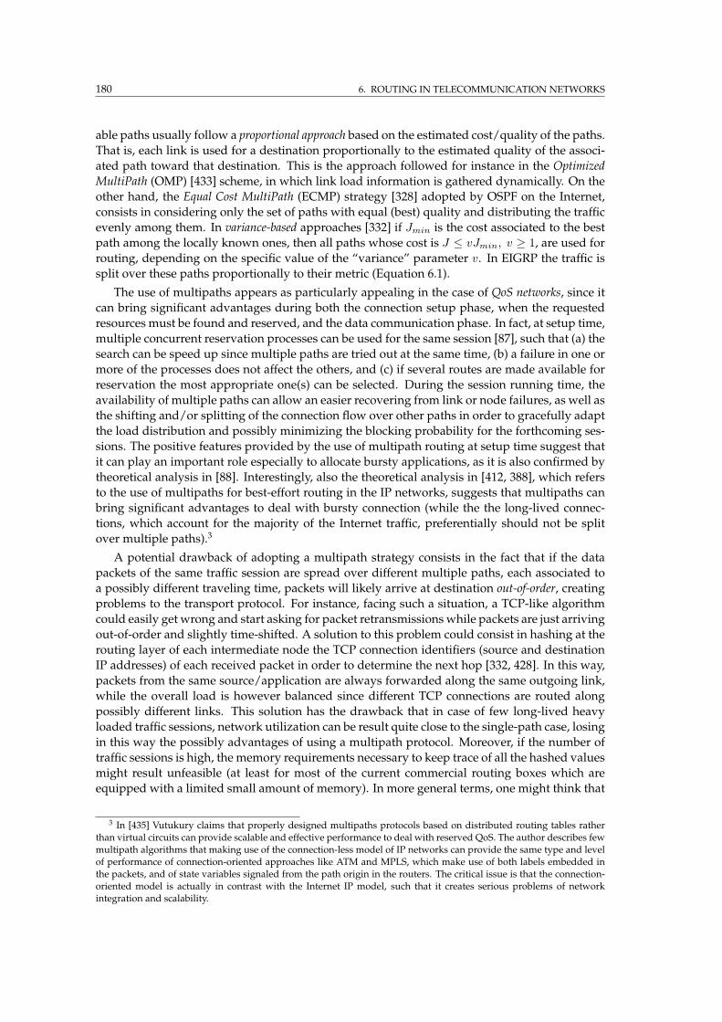
180 6. ROUTING IN TELECOMMUNICATION NETWORKS
able paths usually follow a proportional approach based on the estimated cost/quality of the paths.
That is, each link is used for a destination proportionally to the estimated quality of the associ-
ated path toward that destination. This is the approach followed for instance in the Optimized
MultiPath (OMP) [433] scheme, in which link load information is gathered dynamically. On the
other hand, the Equal Cost MultiPath (ECMP) strategy [328] adopted by OSPF on the Internet,
consists in considering only the set of paths with equal (best) quality and distributing the traffic
evenly among them. In variance-based approaches [332] if Jmin is the cost associated to the best
path among the locally known ones, then all paths whose cost is J ≤ vJmin, v ≥ 1, are used for
routing, depending on the specific value of the “variance” parameter v. In EIGRP the traffic is
split over these paths proportionally to their metric (Equation 6.1).
The use of multipaths appears as particularly appealing in the case of QoS networks, since it
can bring significant advantages during both the connection setup phase, when the requested
resources must be found and reserved, and the data communication phase. In fact, at setup time,
multiple concurrent reservation processes can be used for the same session [87], such that (a) the
search can be speed up since multiple paths are tried out at the same time, (b) a failure in one or
more of the processes does not affect the others, and (c) if several routes are made available for
reservation the most appropriate one(s) can be selected. During the session running time, the
availability of multiple paths can allow an easier recovering from link or node failures, as well as
the shifting and/or splitting of the connection flow over other paths in order to gracefully adapt
the load distribution and possibly minimizing the blocking probability for the forthcoming ses-
sions. The positive features provided by the use of multipath routing at setup time suggest that
it can play an important role especially to allocate bursty applications, as it is also confirmed by
theoretical analysis in [88]. Interestingly, also the theoretical analysis in [412, 388], which refers
to the use of multipaths for best-effort routing in the IP networks, suggests that multipaths can
bring significant advantages to deal with bursty connection (while the the long-lived connec-
tions, which account for the majority of the Internet traffic, preferentially should not be split
over multiple paths).3
A potential drawback of adopting a multipath strategy consists in the fact that if the data
packets of the same traffic session are spread over different multiple paths, each associated to
a possibly different traveling time, packets will likely arrive at destination out-of-order, creating
problems to the transport protocol. For instance, facing such a situation, a TCP-like algorithm
could easily get wrong and start asking for packet retransmissions while packets are just arriving
out-of-order and slightly time-shifted. A solution to this problem could consist in hashing at the
routing layer of each intermediate node the TCP connection identifiers (source and destination
IP addresses) of each received packet in order to determine the next hop [332, 428]. In this way,
packets from the same source/application are always forwarded along the same outgoing link,
while the overall load is however balanced since different TCP connections are routed along
possibly different links. This solution has the drawback that in case of few long-lived heavy
loaded traffic sessions, network utilization can be result quite close to the single-path case, losing
in this way the possibly advantages of using a multipath protocol. Moreover, if the number of
traffic sessions is high, the memory requirements necessary to keep trace of all the hashed values
might result unfeasible (at least for most of the current commercial routing boxes which are
equipped with a limited small amount of memory). In more general terms, one might think that
3 In [435] Vutukury claims that properly designed multipaths protocols based on distributed routing tables ratherthan virtual circuits can provide scalable and effective performance to deal with reserved QoS. The author describes fewmultipath algorithms that making use of the connection-less model of IP networks can provide the same type and levelof performance of connection-oriented approaches like ATM and MPLS, which make use of both labels embedded inthe packets, and of state variables signaled from the path origin in the routers. The critical issue is that the connection-oriented model is actually in contrast with the Internet IP model, such that it creates serious problems of networkintegration and scalability.
6.3 METRICS FOR PERFORMANCE EVALUATION 181
if multipath routing is used then the transport layer algorithms should be consequently adapted
in order to fully exploit the potentialities of using multipaths at the routing layer.
6.3 Metrics for performance evaluation
The performance of a network and, accordingly, of the control algorithms active on it, is mea-
sured according tometrics which depend on the types of services expected to be delivered by the
network. Performance is usually measured over a suitable time interval, and can be expressed
either in terms of instantaneous, cumulative or average values.
In the following the focus is on wired connection-less networks providing best-effort services.
For this class of networks standard metrics for performance evaluation are:
• Throughput: the number of correctly delivered data bits/sec. Throughput is a global index
of performance, associated to the quantity of delivered service. It is usually expressed as the
sum of correctly delivered bits and/or packets over a specified time interval.
• End-to-end delay for data packets: the time necessary to a data packet to reach its destina-
tion node. The values of packet delays can be spread over a wide range. This is an intrinsic
characteristics of data networks: packet delays can range from very low values, for data
flows open between adjacent nodes connected by fast links, to much higher values, in the
case of flows involving nodes very far apart and reachable only through by low band-
width links. Because of this, in the general case, the empirical distribution of packet delays
cannot be expressed in terms of a unimodal parametric distribution. Therefore, mean and
variance of packet delays may not able to capture the most important statistical aspects
of the observed data. Accordingly, in the following, results concerning packet delays are
reported considering also the whole empirical distribution and/or its 90-th percentile.
• Network resources utilization considering both data and routing packets. Network resources
commonly considered are the link capacities and the memory and processing time of the
nodes. Network resources utilization is usually expressed as the used fraction of the over-
all available resources.
In the case of networks providing QoS, additional metrics are usually considered. In princi-
ple, a general and effective way to score the performance of a QoS network is in terms of the total
return that the network provider obtains from all the accepted and correctly routed QoS connec-
tions. That is, the performance can be assessed in terms of the weighted blocking ratio: the number
of accepted (and correctly delivered) traffic sessions multiplied by their associated weight (e.g.,
the monetary return), and divided by the total number of arrived sessions. It is common practice
to considered that the weight is the same for all sessions, such that the objective consists in min-
imizing the number of blocked sessions. This is also the same measure of performance adopted
in the case of telephone networks.
However, in practice the situation is more complex. In fact, usually both best-effort and QoS
traffic coexist, therefore, the negative impact on throughput and packet delays for best-effort
traffic due to the presence of the accepted QoS connections must be also taken into account.
Moreover, users’ pricing strategies can be much more complex than the simple “pay per each
accepted QoS connection”. The whole situation can bemade evenmore intricate by allowing on-
line price negotiations between user applications and the underlying network, such that prices
can vary according to the specific resources requested in relationship to the current, and forth-
coming, traffic load on the network.
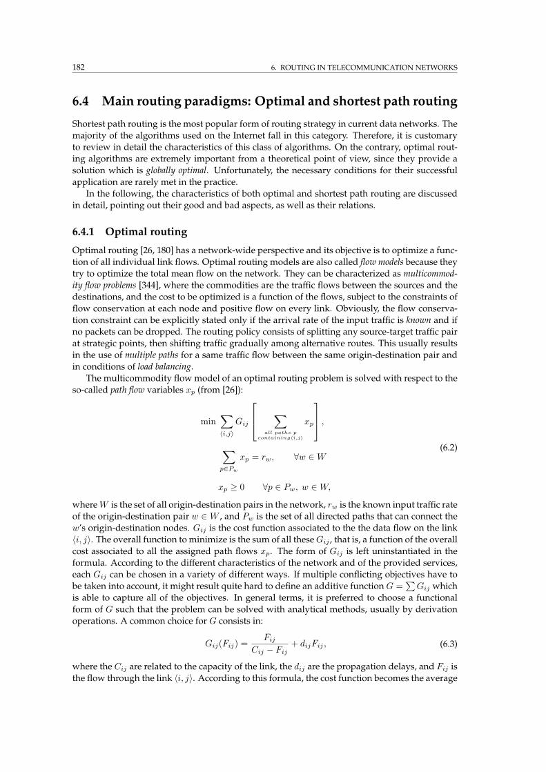
182 6. ROUTING IN TELECOMMUNICATION NETWORKS
6.4 Main routing paradigms: Optimal and shortest path routing
Shortest path routing is the most popular form of routing strategy in current data networks. The
majority of the algorithms used on the Internet fall in this category. Therefore, it is customary
to review in detail the characteristics of this class of algorithms. On the contrary, optimal rout-
ing algorithms are extremely important from a theoretical point of view, since they provide a
solution which is globally optimal. Unfortunately, the necessary conditions for their successful
application are rarely met in the practice.
In the following, the characteristics of both optimal and shortest path routing are discussed
in detail, pointing out their good and bad aspects, as well as their relations.
6.4.1 Optimal routing
Optimal routing [26, 180] has a network-wide perspective and its objective is to optimize a func-
tion of all individual link flows. Optimal routing models are also called flow models because they
try to optimize the total mean flow on the network. They can be characterized as multicommod-
ity flow problems [344], where the commodities are the traffic flows between the sources and the
destinations, and the cost to be optimized is a function of the flows, subject to the constraints of
flow conservation at each node and positive flow on every link. Obviously, the flow conserva-
tion constraint can be explicitly stated only if the arrival rate of the input traffic is known and if
no packets can be dropped. The routing policy consists of splitting any source-target traffic pair
at strategic points, then shifting traffic gradually among alternative routes. This usually results
in the use of multiple paths for a same traffic flow between the same origin-destination pair and
in conditions of load balancing.
The multicommodity flowmodel of an optimal routing problem is solved with respect to the
so-called path flow variables xp (from [26]):
min∑
〈i,j〉
Gij
∑
all paths p
containing〈i,j〉
xp
,
∑
p∈Pw
xp = rw, ∀w ∈W
xp ≥ 0 ∀p ∈ Pw, w ∈W,
(6.2)
whereW is the set of all origin-destination pairs in the network, rw is the known input traffic rate
of the origin-destination pair w ∈ W , and Pw is the set of all directed paths that can connect the
w’s origin-destination nodes. Gij is the cost function associated to the the data flow on the link
〈i, j〉. The overall function to minimize is the sum of all theseGij , that is, a function of the overall
cost associated to all the assigned path flows xp. The form of Gij is left uninstantiated in the
formula. According to the different characteristics of the network and of the provided services,
each Gij can be chosen in a variety of different ways. If multiple conflicting objectives have to
be taken into account, it might result quite hard to define an additive functionG =∑
Gij which
is able to capture all of the objectives. In general terms, it is preferred to choose a functional
form of G such that the problem can be solved with analytical methods, usually by derivation
operations. A common choice for G consists in:
Gij(Fij) =Fij
Cij − Fij+ dijFij , (6.3)
where the Cij are related to the capacity of the link, the dij are the propagation delays, and Fij is
the flow through the link 〈i, j〉. According to this formula, the cost function becomes the average
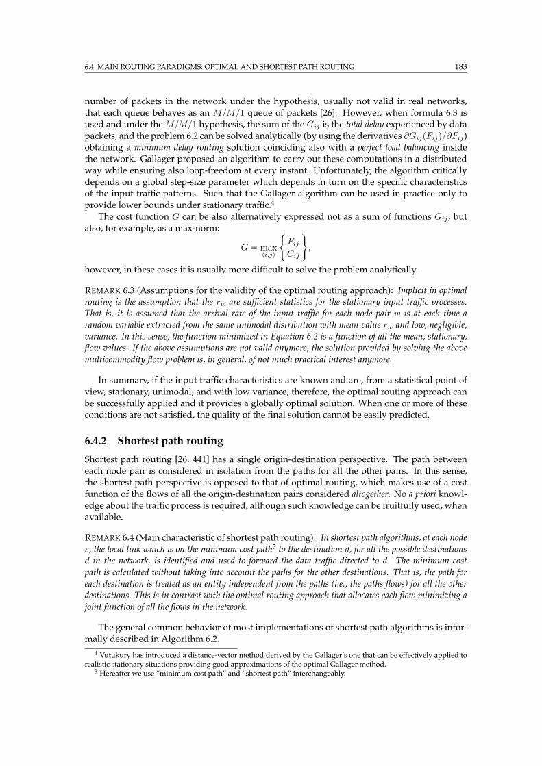
6.4 MAIN ROUTING PARADIGMS: OPTIMAL AND SHORTEST PATH ROUTING 183
number of packets in the network under the hypothesis, usually not valid in real networks,
that each queue behaves as an M/M/1 queue of packets [26]. However, when formula 6.3 is
used and under theM/M/1 hypothesis, the sum of the Gij is the total delay experienced by data
packets, and the problem 6.2 can be solved analytically (by using the derivatives ∂Gij(Fij)/∂Fij)
obtaining a minimum delay routing solution coinciding also with a perfect load balancing inside
the network. Gallager proposed an algorithm to carry out these computations in a distributed
way while ensuring also loop-freedom at every instant. Unfortunately, the algorithm critically
depends on a global step-size parameter which depends in turn on the specific characteristics
of the input traffic patterns. Such that the Gallager algorithm can be used in practice only to
provide lower bounds under stationary traffic.4
The cost function G can be also alternatively expressed not as a sum of functions Gij , but
also, for example, as a max-norm:
G = max〈i,j〉
FijCij
,
however, in these cases it is usually more difficult to solve the problem analytically.
REMARK 6.3 (Assumptions for the validity of the optimal routing approach): Implicit in optimal
routing is the assumption that the rw are sufficient statistics for the stationary input traffic processes.
That is, it is assumed that the arrival rate of the input traffic for each node pair w is at each time a
random variable extracted from the same unimodal distribution with mean value rw and low, negligible,
variance. In this sense, the function minimized in Equation 6.2 is a function of all the mean, stationary,
flow values. If the above assumptions are not valid anymore, the solution provided by solving the above
multicommodity flow problem is, in general, of not much practical interest anymore.
In summary, if the input traffic characteristics are known and are, from a statistical point of
view, stationary, unimodal, and with low variance, therefore, the optimal routing approach can
be successfully applied and it provides a globally optimal solution. When one or more of these
conditions are not satisfied, the quality of the final solution cannot be easily predicted.
6.4.2 Shortest path routing
Shortest path routing [26, 441] has a single origin-destination perspective. The path between
each node pair is considered in isolation from the paths for all the other pairs. In this sense,
the shortest path perspective is opposed to that of optimal routing, which makes use of a cost
function of the flows of all the origin-destination pairs considered altogether. No a priori knowl-
edge about the traffic process is required, although such knowledge can be fruitfully used, when
available.
REMARK 6.4 (Main characteristic of shortest path routing): In shortest path algorithms, at each node
s, the local link which is on the minimum cost path5 to the destination d, for all the possible destinations
d in the network, is identified and used to forward the data traffic directed to d. The minimum cost
path is calculated without taking into account the paths for the other destinations. That is, the path for
each destination is treated as an entity independent from the paths (i.e., the paths flows) for all the other
destinations. This is in contrast with the optimal routing approach that allocates each flow minimizing a
joint function of all the flows in the network.
The general common behavior of most implementations of shortest path algorithms is infor-
mally described in Algorithm 6.2.
4 Vutukury has introduced a distance-vector method derived by the Gallager’s one that can be effectively applied torealistic stationary situations providing good approximations of the optimal Gallager method.
5 Hereafter we use “minimum cost path” and “shortest path” interchangeably.
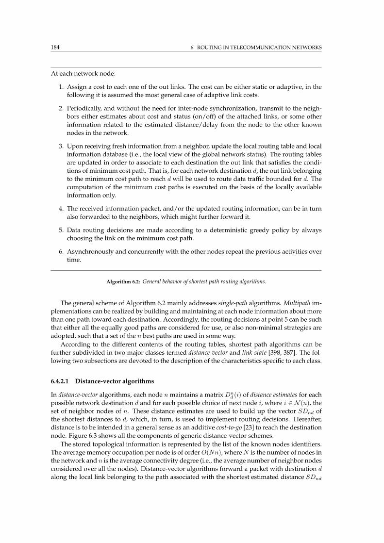
184 6. ROUTING IN TELECOMMUNICATION NETWORKS
At each network node:
1. Assign a cost to each one of the out links. The cost can be either static or adaptive, in the
following it is assumed the most general case of adaptive link costs.
2. Periodically, and without the need for inter-node synchronization, transmit to the neigh-
bors either estimates about cost and status (on/off) of the attached links, or some other
information related to the estimated distance/delay from the node to the other known
nodes in the network.
3. Upon receiving fresh information from a neighbor, update the local routing table and local
information database (i.e., the local view of the global network status). The routing tables
are updated in order to associate to each destination the out link that satisfies the condi-
tions of minimum cost path. That is, for each network destination d, the out link belonging
to the minimum cost path to reach d will be used to route data traffic bounded for d. The
computation of the minimum cost paths is executed on the basis of the locally available
information only.
4. The received information packet, and/or the updated routing information, can be in turn
also forwarded to the neighbors, which might further forward it.
5. Data routing decisions are made according to a deterministic greedy policy by always
choosing the link on the minimum cost path.
6. Asynchronously and concurrently with the other nodes repeat the previous activities over
time.
Algorithm 6.2: General behavior of shortest path routing algorithms.
The general scheme of Algorithm 6.2 mainly addresses single-path algorithms. Multipath im-
plementations can be realized by building andmaintaining at each node information about more
than one path toward each destination. Accordingly, the routing decisions at point 5 can be such
that either all the equally good paths are considered for use, or also non-minimal strategies are
adopted, such that a set of the n best paths are used in some way.
According to the different contents of the routing tables, shortest path algorithms can be
further subdivided in two major classes termed distance-vector and link-state [398, 387]. The fol-
lowing two subsections are devoted to the description of the characteristics specific to each class.
6.4.2.1 Distance-vector algorithms
In distance-vector algorithms, each node n maintains a matrix Dnd (i) of distance estimates for each
possible network destination d and for each possible choice of next node i, where i ∈ N (n), the
set of neighbor nodes of n. These distance estimates are used to build up the vector SDnd of
the shortest distances to d, which, in turn, is used to implement routing decisions. Hereafter,
distance is to be intended in a general sense as an additive cost-to-go [23] to reach the destination
node. Figure 6.3 shows all the components of generic distance-vector schemes.
The stored topological information is represented by the list of the known nodes identifiers.
The average memory occupation per node is of orderO(Nn), whereN is the number of nodes in
the network and n is the average connectivity degree (i.e., the average number of neighbor nodes
considered over all the nodes). Distance-vector algorithms forward a packet with destination d
along the local link belonging to the path associated with the shortest estimated distance SDnd
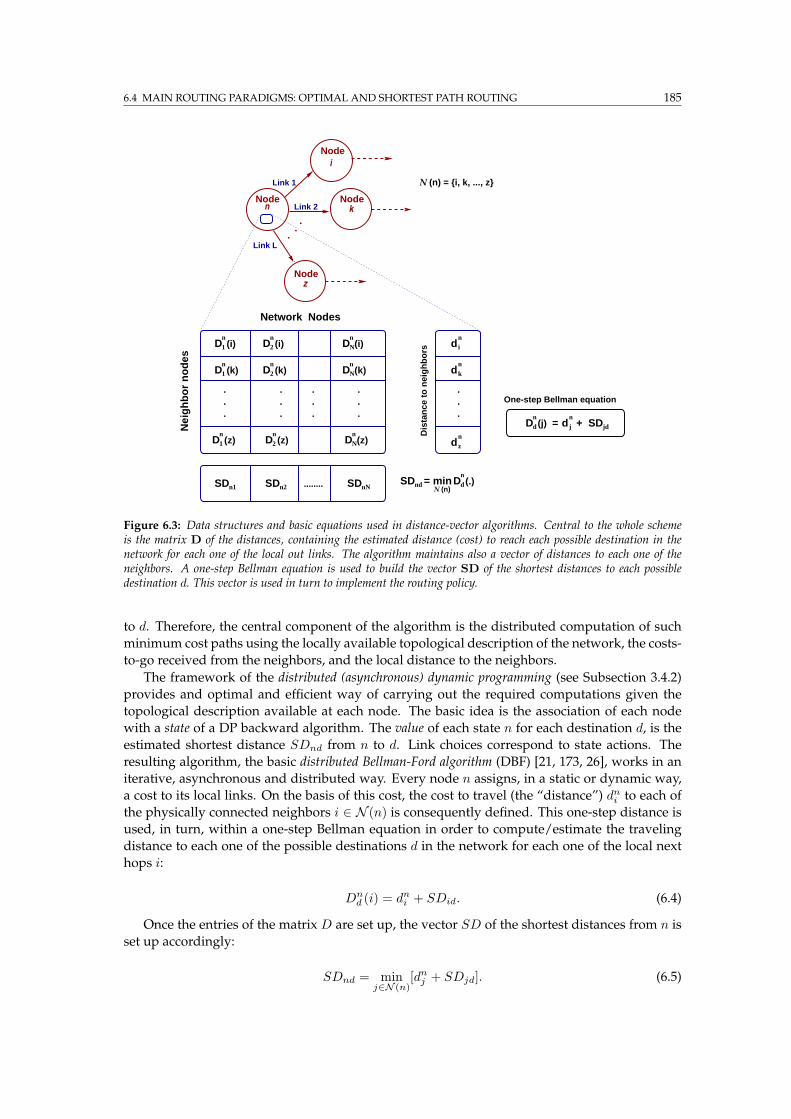
6.4 MAIN ROUTING PARADIGMS: OPTIMAL AND SHORTEST PATH ROUTING 185
nN
n1 (i)
ni
nk
nz
n(z)N
n1 n2 N (n)
nd (.)
nd (j)
nj jd
N (n) = i, k, ..., z
n(i)
n(i)
n2 (k)
nN(k)
n1 (z)
n2
n1 (k)
2 N
(z)
nd
. . .
........ SD = min SD
D d
d
dD
SD SD D
D d SD= +
Node n
. . . . . . . .
. . . .
Node
Node kLink 2
Link 1
Link L
Dis
tan
ce t
o n
eig
hb
ors
i
Nei
gh
bo
r n
od
es
Network Nodes
D D
D D
D D
D
Node z
. .
.
One-step Bellman equation
Figure 6.3: Data structures and basic equations used in distance-vector algorithms. Central to the whole schemeis the matrix D of the distances, containing the estimated distance (cost) to reach each possible destination in thenetwork for each one of the local out links. The algorithm maintains also a vector of distances to each one of theneighbors. A one-step Bellman equation is used to build the vector SD of the shortest distances to each possibledestination d. This vector is used in turn to implement the routing policy.
to d. Therefore, the central component of the algorithm is the distributed computation of such
minimum cost paths using the locally available topological description of the network, the costs-
to-go received from the neighbors, and the local distance to the neighbors.
The framework of the distributed (asynchronous) dynamic programming (see Subsection 3.4.2)
provides and optimal and efficient way of carrying out the required computations given the
topological description available at each node. The basic idea is the association of each node
with a state of a DP backward algorithm. The value of each state n for each destination d, is the
estimated shortest distance SDnd from n to d. Link choices correspond to state actions. The
resulting algorithm, the basic distributed Bellman-Ford algorithm (DBF) [21, 173, 26], works in an
iterative, asynchronous and distributed way. Every node n assigns, in a static or dynamic way,
a cost to its local links. On the basis of this cost, the cost to travel (the “distance”) dni to each of
the physically connected neighbors i ∈ N (n) is consequently defined. This one-step distance is
used, in turn, within a one-step Bellman equation in order to compute/estimate the traveling
distance to each one of the possible destinations d in the network for each one of the local next
hops i:
Dnd (i) = dni + SDid. (6.4)
Once the entries of the matrix D are set up, the vector SD of the shortest distances from n is
set up accordingly:
SDnd = minj∈N (n)
[dnj + SDjd]. (6.5)
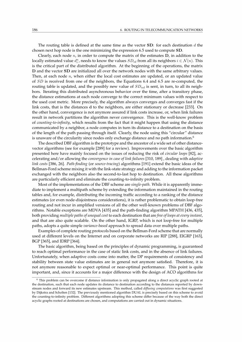
186 6. ROUTING IN TELECOMMUNICATION NETWORKS
The routing table is defined at the same time as the vector SD: for each destination d the
chosen next hop node is the one minimizing the expression 6.5 used to compute SD.
Clearly, each node n, in order to compute the matrix of the estimates D, in addition to the
locally estimated value dni , needs to know the values SDid from all its neighbors i ∈ N (n). This
is the critical part of the distributed algorithm. At the beginning of the operations, the matrix
D and the vector SD are initialized all over the network nodes with the same arbitrary values.
Then, at each node n, when either the local cost estimates are updated, or an updated value
of SD is received from one of the neighbors, the Equations 6.4 and 6.5 are re-computed, the
routing table is updated, and the possibly new value of SDnd is sent, in turn, to all its neigh-
bors. Iterating this distributed asynchronous behavior over the time, after a transitory phase,
the distance estimations at each node converge to the correct minimum values with respect to
the used cost metric. More precisely, the algorithm always converges and converges fast if the
link costs, that is the distances d to the neighbors, are either stationary or decrease [233]. On
the other hand, convergence is not anymore assured if link costs increase, or, when link failures
result in network partitions the algorithm never convergence. This is the well-know problem
of counting-to-infinity, which results from the fact that it might happen that using the distance
communicated by a neighbor, a node computes in turn its distance to a destination on the basis
of the length of the path passing through itself. Clearly, the node using this “circular” distance
is unaware of the circularity since nodes only exchange distance and no path information.6
The describedDBF algorithm is the prototype and the ancestor of awide set of other distance-
vector algorithms (see for example [289] for a review). Improvements over the basic algorithm
presented here have mainly focused on the issues of reducing the risk of circular loops [82], ac-
celerating and/or allowing the convergence in case of link failures [310, 189] , dealing with adaptive
link costs [386, 26]. Path-finding (or source-tracing) algorithms [191] extend the basic ideas of the
Bellman-Ford schememixing it with the link-state strategy and adding to the information packet
exchanged with the neighbors also the second-to-last hop to destination. All these algorithms
are particularly efficient and eliminate the counting-to-infinity problem.
Most of the implementations of the DBF scheme are single-path. While it is apparently imme-
diate to implement a multipath scheme by extending the information maintained in the routing
tables and, for example, distributing the incoming traffic according to a ranking of the distance
estimates (or even node-disjointness considerations), it is rather problematic to obtain loop-free
routing and not incur in amplified versions of all the other well-known problems of DBF algo-
rithms. Notable exceptions are MDVA [435] and the path-finding algorithm MPATH [436, 435],
both providingmultiple paths of unequal cost to each destination that are free of loops at every instant,
and that are also quite scalable. On the other hand, IGRP, which is not loop-free for multiple
paths, adopts a quite simple variance-based approach to spread data over multiple paths.
Examples of complete routing protocols based on the Bellman-Ford scheme that are normally
used at different levels on the Internet and on corporate networks are RIP [288], EIGRP [163],
BGP [365], and IDRP [364].
The basic algorithm, being based on the principles of dynamic programming, is guaranteed
to reach optimal performance in the case of static link costs, and in the absence of link failures.
Unfortunately, when adaptive costs come into matter, the DP requirements of consistency and
stability between state value estimates are in general not anymore satisfied. Therefore, it is
not anymore reasonable to expect optimal or near-optimal performance. This point is quite
important, and, since it accounts for a major difference with the design of ACO algorithms for
6 This problem can be overcome if distance information is only propagated along a direct acyclic graph rooted atthe destination, such that each node updates its distance to destination according to the distances reported by down-stream nodes and forward its new estimates upstream. This method, called diffusing computations was first suggestedby Dijkstra and Scholten [132]. The previously mentioned algorithm DUAL is precisely based on this scheme to avoidthe counting-to-infinity problem. Different algorithms adopting this scheme differ because of the way both the directacyclic graphs rooted at destinations are chosen, and computations are carried out in dynamic situations.
6.4 MAIN ROUTING PARADIGMS: OPTIMAL AND SHORTEST PATH ROUTING 187
routing, it is useful to clarify here which is, in general, the problem of following a DP approach
in the case of a dynamic and distributed environment.
As discussed in Subsection 3.4.2, DP makes use of information bootstrapping to efficiently ex-
ploit the Markov structure of the state space and update the cost-to-go of one state using the
costs-to-go of predecessor states. In order to work properly, bootstrapping requires stationar-
ity and the fact that the Markov property holds. To show the potential problems with the DP
approach, let us consider the following situation:
EXAMPLE 6.1: DRAWBACKS OF USING DYNAMIC PROGRAMMING IN DYNAMIC NETWORKS
Let start with node n sending to its neighbor i the current shortest distance estimate SDnd for destination
d. On receiving the information packet from n, node i updates, its distance estimate for destination d by
applying the one-step Bellman equation. Let the path through node n becoming the shortest one to reach
destination d from i. Therefore, i, in turn, sends its new SDid to the neighbors, that will make their
updates, and, in turn, will possibly propagate the new distance estimates. After some time steps, all the
nodes in the network will have their distance estimates for destination d updated. Now, let us imagine
that the position of node n is such that all the paths for d pass now through n, and that after a while a new
user application starts at node n sending data to i, therefore jamming the link that node n is currently
using to forward data towards d. At this point, node n must: (i) get aware of the changed situation, (ii)
trigger an update of the link costs, (iii) update its distance estimate SDnd about destination d, that will
likely be much higher than before. Once the distance estimate has been updated, it must be transmitted to
i, that in turn, will transmit it to its neighbors and so on, until all the nodes in the network can get aware
of the changed traffic situation and change the routing paths accordingly. During all this updating time,
all the distance estimates over the whole network are potentially inconsistent. It takes some relaxation
time before the estimates become jointly consistent again. In principle, if there are continual oscillations
in the adaptive values of the local link costs, the distance estimates never get consistent, with an expected
negative impact on the overall performance when bootstrapping is used. On the contrary, if link costs are
calculated in an adaptive way but their vales are smoothed adopting a low-pass filter, the local oscillations
are damped out and distance estimates are in general more consistent. In this case bootstrapping can be
safely used, but the algorithm will result much less adaptive.
Bootstrapping is a powerful technique in the static and Markov case. It allows to save a lot
of computation by propagating estimates from one node to all the other nodes. A single cost
update allows the update of the distance estimates of virtually all the nodes in the network, but,
on the other hand:
REMARK 6.5 (Bootstrapping and globally wrong routing tables): In the adaptive, non-stationary
case, bootstrapping can also mean that one wrong estimate, wrong because of the lack of global view at
the nodes or of high non-stationarity in the input traffic, is propagated, step-by-step, to all the other nodes
in the networks, determining, in principle, a routing policy which is wrong across the whole the network.
ACO algorithms routing, do not rely on bootstrapping, even if it can be used in principle.
Instead, Monte Carlo updates are used. This design choice makes in general ACO algorithms
less effective in the stationary case, with respect to a typical Bellman-Ford algorithm, but more
robust and better performing in the more interesting non-stationary case.
6.4.2.2 Link-state algorithms
Link-state algorithms make use of routing tables containing much more information than that
used in distance-vector algorithms:

188 6. ROUTING IN TELECOMMUNICATION NETWORKS
REMARK 6.6 (Characteristics of link-state algorithms): At the core of link-state algorithms there is a
distributed and replicated database. This database is essentially a topological map, usually built in a
dynamic way, of the whole network. The map contains comprehensive information concerning the link-
state of the links of all the network nodes, that is, information about their cost value, node end-points, and
operational status. Figure 6.4 schematically shows such an organization.
TableRouting
TableRouting
TableRouting
TableRouting
TableRouting
Figure 6.4: Schematic representation of the topological information used in link-state algorithms. Each node on thesame hierarchical level maintains a complete description of the link states (costs, interconnections, operational status)of all the network nodes that belong to the same hierarchical level.
In order to avoid this local database to grow up linearly with the size of the whole network,
as well as for other general administrative and logistic reasons, networks usually have a hierar-
chical organization. Therefore, the link-state maps need to contain only information related to the
network nodes on the same hierarchical level. Hierarchical organization is an important aspect
of the whole network management. For example, in the Internet, nodes are organized in hier-
archical Autonomous Systems and multiple routing areas inside each Autonomous System [328].
Roughly speaking, sub-networks are seen as single host nodes connected to interface nodes
called gateways. Gateways perform fairly sophisticated network layer tasks, including routing.
Groups of gateways, connected by an arbitrary topology, define logical areas. Inside each area, all
the gateways are at the same hierarchical level and flat routing is performed among them. Areas
communicate only by means of area border gateways. In this way, the computational complex-
ity of the routing problem itself, as seen by each gateway, is much reduced (e.g., OSPF areas in
the Internet typically group from 10 to 300 gateways), while the complexity of the design and
management of the routing protocol is much increased. These considerations are in general not to
limited to link-state algorithms, but are valid for any type of routing scheme.
Using the local link-state description as input, each node can calculate shortest paths from
itself to each destination node by using any classical algorithm for centralized shortest path
computations. Typically, some efficient variant of the basic Dijkstra’s algorithm [131] is used.
The memory requirement for each node in this case is O(N2), that has to be compared to the
average value of O(Nm) for the distance-vector case. The main difference between the two
algorithmic schemes lies exactly in the information locally available to each node to compute
the shortest paths. Distance-vector algorithms carry out the computation in a distributed way
involving all the network nodes, while in link-state algorithms every single node carries out
an independent centralized computation of the shortest paths. Therefore, link-state algorithms
require locally both more computational power and more memory space, but can provide also
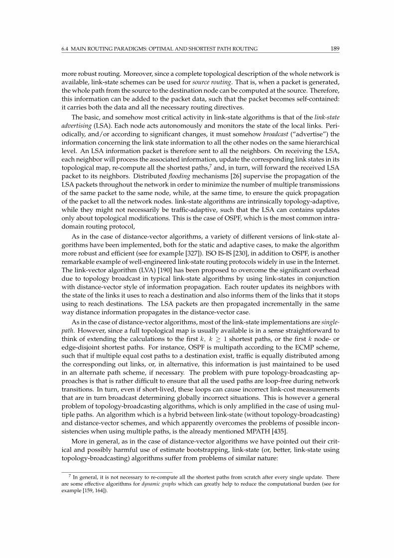
6.4 MAIN ROUTING PARADIGMS: OPTIMAL AND SHORTEST PATH ROUTING 189
more robust routing. Moreover, since a complete topological description of the whole network is
available, link-state schemes can be used for source routing. That is, when a packet is generated,
the whole path from the source to the destination node can be computed at the source. Therefore,
this information can be added to the packet data, such that the packet becomes self-contained:
it carries both the data and all the necessary routing directives.
The basic, and somehow most critical activity in link-state algorithms is that of the link-state
advertising (LSA). Each node acts autonomously and monitors the state of the local links. Peri-
odically, and/or according to significant changes, it must somehow broadcast (“advertise”) the
information concerning the link state information to all the other nodes on the same hierarchical
level. An LSA information packet is therefore sent to all the neighbors. On receiving the LSA,
each neighbor will process the associated information, update the corresponding link states in its
topological map, re-compute all the shortest paths,7 and, in turn, will forward the received LSA
packet to its neighbors. Distributed flooding mechanisms [26] supervise the propagation of the
LSA packets throughout the network in order to minimize the number of multiple transmissions
of the same packet to the same node, while, at the same time, to ensure the quick propagation
of the packet to all the network nodes. link-state algorithms are intrinsically topology-adaptive,
while they might not necessarily be traffic-adaptive, such that the LSA can contains updates
only about topological modifications. This is the case of OSPF, which is the most common intra-
domain routing protocol,
As in the case of distance-vector algorithms, a variety of different versions of link-state al-
gorithms have been implemented, both for the static and adaptive cases, to make the algorithm
more robust and efficient (see for example [327]). ISO IS-IS [230], in addition to OSPF, is another
remarkable example of well-engineered link-state routing protocols widely in use in the Internet.
The link-vector algorithm (LVA) [190] has been proposed to overcome the significant overhead
due to topology broadcast in typical link-state algorithms by using link-states in conjunction
with distance-vector style of information propagation. Each router updates its neighbors with
the state of the links it uses to reach a destination and also informs them of the links that it stops
using to reach destinations. The LSA packets are then propagated incrementally in the same
way distance information propagates in the distance-vector case.
As in the case of distance-vector algorithms, most of the link-state implementations are single-
path. However, since a full topological map is usually available is in a sense straightforward to
think of extending the calculations to the first k, k ≥ 1 shortest paths, or the first k node- or
edge-disjoint shortest paths. For instance, OSPF is multipath according to the ECMP scheme,
such that if multiple equal cost paths to a destination exist, traffic is equally distributed among
the corresponding out links, or, in alternative, this information is just maintained to be used
in an alternate path scheme, if necessary. The problem with pure topology-broadcasting ap-
proaches is that is rather difficult to ensure that all the used paths are loop-free during network
transitions. In turn, even if short-lived, these loops can cause incorrect link-cost measurements
that are in turn broadcast determining globally incorrect situations. This is however a general
problem of topology-broadcasting algorithms, which is only amplified in the case of using mul-
tiple paths. An algorithm which is a hybrid between link-state (without topology-broadcasting)
and distance-vector schemes, and which apparently overcomes the problems of possible incon-
sistencies when using multiple paths, is the already mentioned MPATH [435].
More in general, as in the case of distance-vector algorithms we have pointed out their crit-
ical and possibly harmful use of estimate bootstrapping, link-state (or, better, link-state using
topology-broadcasting) algorithms suffer from problems of similar nature:
7 In general, it is not necessary to re-compute all the shortest paths from scratch after every single update. Thereare some effective algorithms for dynamic graphs which can greatly help to reduce the computational burden (see forexample [159, 164]).
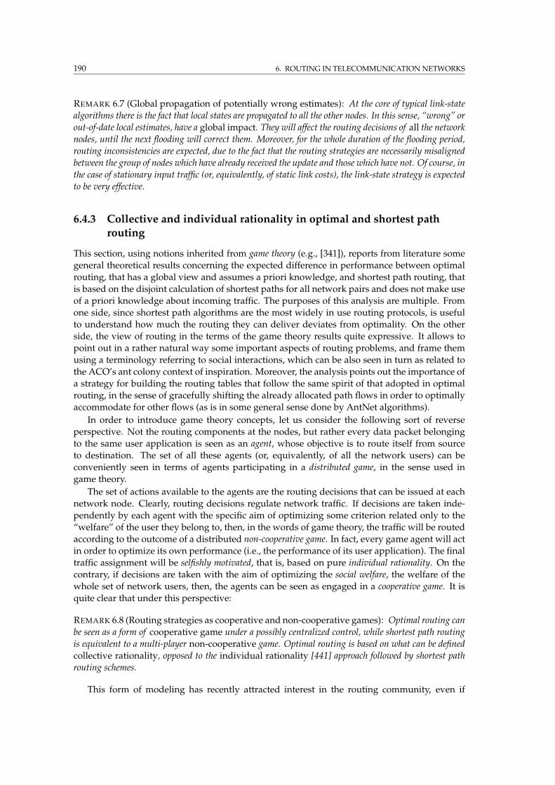
190 6. ROUTING IN TELECOMMUNICATION NETWORKS
REMARK 6.7 (Global propagation of potentially wrong estimates): At the core of typical link-state
algorithms there is the fact that local states are propagated to all the other nodes. In this sense, “wrong” or
out-of-date local estimates, have a global impact. They will affect the routing decisions of all the network
nodes, until the next flooding will correct them. Moreover, for the whole duration of the flooding period,
routing inconsistencies are expected, due to the fact that the routing strategies are necessarily misaligned
between the group of nodes which have already received the update and those which have not. Of course, in
the case of stationary input traffic (or, equivalently, of static link costs), the link-state strategy is expected
to be very effective.
6.4.3 Collective and individual rationality in optimal and shortest path
routing
This section, using notions inherited from game theory (e.g., [341]), reports from literature some
general theoretical results concerning the expected difference in performance between optimal
routing, that has a global view and assumes a priori knowledge, and shortest path routing, that
is based on the disjoint calculation of shortest paths for all network pairs and does not make use
of a priori knowledge about incoming traffic. The purposes of this analysis are multiple. From
one side, since shortest path algorithms are the most widely in use routing protocols, is useful
to understand how much the routing they can deliver deviates from optimality. On the other
side, the view of routing in the terms of the game theory results quite expressive. It allows to
point out in a rather natural way some important aspects of routing problems, and frame them
using a terminology referring to social interactions, which can be also seen in turn as related to
the ACO’s ant colony context of inspiration. Moreover, the analysis points out the importance of
a strategy for building the routing tables that follow the same spirit of that adopted in optimal
routing, in the sense of gracefully shifting the already allocated path flows in order to optimally
accommodate for other flows (as is in some general sense done by AntNet algorithms).
In order to introduce game theory concepts, let us consider the following sort of reverse
perspective. Not the routing components at the nodes, but rather every data packet belonging
to the same user application is seen as an agent, whose objective is to route itself from source
to destination. The set of all these agents (or, equivalently, of all the network users) can be
conveniently seen in terms of agents participating in a distributed game, in the sense used in
game theory.
The set of actions available to the agents are the routing decisions that can be issued at each
network node. Clearly, routing decisions regulate network traffic. If decisions are taken inde-
pendently by each agent with the specific aim of optimizing some criterion related only to the
“welfare” of the user they belong to, then, in the words of game theory, the traffic will be routed
according to the outcome of a distributed non-cooperative game. In fact, every game agent will act
in order to optimize its own performance (i.e., the performance of its user application). The final
traffic assignment will be selfishly motivated, that is, based on pure individual rationality. On the
contrary, if decisions are taken with the aim of optimizing the social welfare, the welfare of the
whole set of network users, then, the agents can be seen as engaged in a cooperative game. It is
quite clear that under this perspective:
REMARK 6.8 (Routing strategies as cooperative and non-cooperative games): Optimal routing can
be seen as a form of cooperative game under a possibly centralized control, while shortest path routing
is equivalent to a multi-player non-cooperative game. Optimal routing is based on what can be defined
collective rationality, opposed to the individual rationality [441] approach followed by shortest path
routing schemes.
This form of modeling has recently attracted interest in the routing community, even if
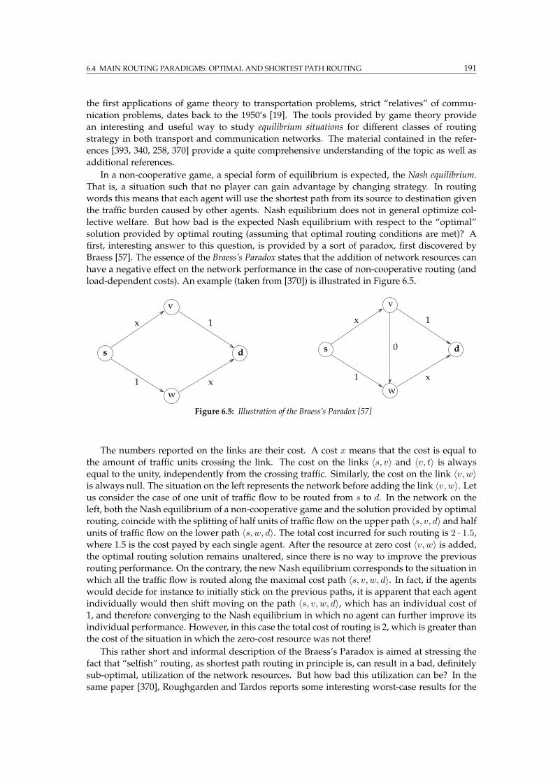
6.4 MAIN ROUTING PARADIGMS: OPTIMAL AND SHORTEST PATH ROUTING 191
the first applications of game theory to transportation problems, strict “relatives” of commu-
nication problems, dates back to the 1950’s [19]. The tools provided by game theory provide
an interesting and useful way to study equilibrium situations for different classes of routing
strategy in both transport and communication networks. The material contained in the refer-
ences [393, 340, 258, 370] provide a quite comprehensive understanding of the topic as well as
additional references.
In a non-cooperative game, a special form of equilibrium is expected, the Nash equilibrium.
That is, a situation such that no player can gain advantage by changing strategy. In routing
words this means that each agent will use the shortest path from its source to destination given
the traffic burden caused by other agents. Nash equilibrium does not in general optimize col-
lective welfare. But how bad is the expected Nash equilibrium with respect to the “optimal”
solution provided by optimal routing (assuming that optimal routing conditions are met)? A
first, interesting answer to this question, is provided by a sort of paradox, first discovered by
Braess [57]. The essence of the Braess’s Paradox states that the addition of network resources can
have a negative effect on the network performance in the case of non-cooperative routing (and
load-dependent costs). An example (taken from [370]) is illustrated in Figure 6.5.
s d
x
1 x
1
w
v
s d
x
1 x
1
0
v
w
Figure 6.5: Illustration of the Braess’s Paradox [57]
The numbers reported on the links are their cost. A cost x means that the cost is equal to
the amount of traffic units crossing the link. The cost on the links 〈s, v〉 and 〈v, t〉 is always
equal to the unity, independently from the crossing traffic. Similarly, the cost on the link 〈v, w〉is always null. The situation on the left represents the network before adding the link 〈v, w〉. Letus consider the case of one unit of traffic flow to be routed from s to d. In the network on the
left, both the Nash equilibrium of a non-cooperative game and the solution provided by optimal
routing, coincide with the splitting of half units of traffic flow on the upper path 〈s, v, d〉 and half
units of traffic flow on the lower path 〈s, w, d〉. The total cost incurred for such routing is 2 · 1.5,where 1.5 is the cost payed by each single agent. After the resource at zero cost 〈v, w〉 is added,the optimal routing solution remains unaltered, since there is no way to improve the previous
routing performance. On the contrary, the newNash equilibrium corresponds to the situation in
which all the traffic flow is routed along the maximal cost path 〈s, v, w, d〉. In fact, if the agents
would decide for instance to initially stick on the previous paths, it is apparent that each agent
individually would then shift moving on the path 〈s, v, w, d〉, which has an individual cost of
1, and therefore converging to the Nash equilibrium in which no agent can further improve its
individual performance. However, in this case the total cost of routing is 2, which is greater than
the cost of the situation in which the zero-cost resource was not there!
This rather short and informal description of the Braess’s Paradox is aimed at stressing the
fact that “selfish” routing, as shortest path routing in principle is, can result in a bad, definitely
sub-optimal, utilization of the network resources. But how bad this utilization can be? In the
same paper [370], Roughgarden and Tardos reports some interesting worst-case results for the
192 6. ROUTING IN TELECOMMUNICATION NETWORKS
performance of selfish routing, under some specific and restrictive assumptions and conditions
on the traffic flows and the characteristics of the link costs. The probably most interesting result,
which is reported here without the otherwise necessary mathematical details, states that:
REMARK 6.9 (Worst-case performance for shortest path strategies): A traffic flow at (the unique)
Nash equilibrium has a total cost, expressed in terms of link latency, no more than that incurred by the
solution provided by optimal routing in the case of a traffic flow double of that flow.
In spite of the limited practical applicability of the result, considered the specific restrictions
that have been assumed, this result gives the “flavor” that shortest path routing cannot be ar-
bitrarily worse than optimal routing. Moreover, it indicates the fact that adding cooperation
among the agents can, in principle, greatly improve the performance, because it can be possible
to go beyond the performance limits of (selfish) Nash equilibria. Where cooperation can be seen
in the terms of the ability to repeatedly and gradually adjust the path flows in order to take into
the right account the existence of the other paths flows, realizing over time a sort of relaxation
process that would mimic the global strategy adopted by optimal routing to assign the path
flows. That is:
REMARK 6.10 (Approximate optimal routing performance): The performance of optimal routing can
be expected to be approached by a cost-adaptive strategy that gracefully remodels over time the routing
tables according to both local and non-local perspective and that is not fully greedy in the sense of always
deterministically following the minimum cost shortest paths. The design of our ACO algorithms for
routing precisely go in this direction, since they feature adaptivity, multiple paths, stochastic decisions,
and remote information sampling.
The statedworst-case result for the performance of shortest path routing is based on the usual
assumption that a priori knowledge about the input traffic is not available to the shortest path
algorithm. Although, it could be fruitfully used if available. Moreover, is in a sense more fair to
compare optimal and shortest path routing assuming the same amount of a priori knowledge.
In this case, shortest path can in principle provide precisely the same performance as optimal
routing once the knowledge about the statistical characteristics on incoming traffic in used to set
the costs of the links, such that the solution provided by the shortest path algorithm can be the
same as that obtainable by applying optimal routing.
REMARK 6.11 (The problem of setting optimal link costs is NP-hard): Given the knowledge about
the input traffic, search for an assignment of link costs such that the shortest-path solution is the same as
the one obtainable by optimal routing. This is a sort of inverse problem that once solved could be used
for instance on the Internet, where, for several practical reasons other than pure routing performance (e.g.,
the complete independence among the nodes), shortest-path routing is used. Unfortunately, this inverse
problem is NP-hard [174].
Therefore, if in principle, under the above specific conditions, shortest-path routing can
be the same as optimal routing, in practice this results computationally unfeasible. A good
overview on the problem, and an effective genetic algorithm heuristic is provided in [284].
6.5 An historical glance at the routing on the Internet
For the management of routing on the Internet and on its predecessor, ARPANET, several im-
plementations of shortest path protocols have been used over the years.
The first ARPANET routing algorithm (1969) was a distributed adaptive asynchronous Bellman-
Ford algorithm [26]. It used an adaptive link cost metric based on local measures of traffic con-
gestion on the links and in particular on the number of packets waiting in the link queues. The
6.5 AN HISTORICAL GLANCE AT THE ROUTING ON THE INTERNET 193
chosen adaptive metric led to considerable oscillations, such that a large positive constant value
was added to each link cost in order to stabilize the oscillations. Unfortunately, this solution
dramatically reduced the sensitivity to traffic congestion situations.
These problems led, in 1980, to a second version of the routing algorithm on ARPANET, a
link-state routing algorithm known as Shortest Path First (SPF) [304]. An adaptive link cost metric
was still used, based on local statistics of the delays experienced by data packets. Cost were
defined in term of transmission delays by summing queuing, transmission and propagation
delays.
This new class of algorithms exhibited more robust behavior than previous distance-vector
algorithms, but, in this case too, under heavy load conditions, the observed oscillations were too
large. Several changes were operated in order to limit the allowed variability in the link cost
values [252, 453].
Through the years, the ARPANET was transformed in NSFNET, and progressively trans-
formed from a USA network to a world network, becoming the Internet as we know it today.
With the increasing of the global connectivity, there was an explosion of administrative and
management problems. Nowadays, Internet is a very complex system, organized at several
hierarchical levels and managed by several organizations spread all over the globe. This ever
increasing level of complexity, asked for routing algorithms with stable performance and for
routing protocols able to deal with efficiency and safeness with the explosion of topological
complexity. It is in this perspective, that the first adaptive attempts have been ruled out. The
current routing algorithms used on the Internet, both distance-vector and link-state, are mainly
topology-adaptive, but not really traffic-adaptive. Moreover, they are mostly single-path al-
gorithms implementing only quite limited form of multi-path routing. This is the case of the
already mentioned OSPF [328], which is a link-state protocol widely in use as Interior Gateway
Protocol (IGP) and Border Gateway Protocol (BGP), that is, for inter- and intra-areas routing.
Also RIP [288, 289] can be and is used in both situations, anyhow, OSPF is more appropriate for
larger Autonomous Systems.8
This very short historical retrospective highlights the many difficulties encountered in the
implementation of adaptive and possibly multi-path routing algorithms for the Internet. The
current Internet routing system is not clearly the “best solution”: is probably the “best compro-
mise” among efficiency, stability and robustness that has been found so far. A great amount of
the complexity concerning the control of the network dynamics has been de facto moved from
the routing layer to the transport layer, where the TCP [93] supervises both reliable end-to-end
data transfers and congestion control.
In order to further support the design ideas that will be behind our AntNet, is appropriate to
conclude this section with the following consideration:
REMARK 6.12 (The need for adaptive multipath algorithms): Even if adaptive routing “failed” in
the past, the need for an adaptive and efficient routing system on the Internet is virtually still there. In
particular, in the present/future scenario of networks massively providing both best-effort and QoS, it
will be of primary importance to have efficient routing policies able to discover, allocate and maintain
routing paths in a business-effective way. In this perspective, the adoption of fully adaptive multi-path
algorithms seems to be the right way of dealing with the problems, as also pointed out by several recent
studies (e.g., [332, 435, 436, 88, 77, 388]).
8 Node systems on the same hierarchical level should not exceed the few hundred nodes, as CISCO, one of the worldleaders in network technologies, suggests, in order to keep performance at a good level given the characteristics ofcurrently in use switching and transmission technology.
194 6. ROUTING IN TELECOMMUNICATION NETWORKS
6.6 Summary
This chapter has discussed several issues that are central for routing. The contents of the chapter
are complemented by Appendix F which reports about general characteristics of telecommuni-
cation networks (layered architectures, transmission technologies, delivered services, etc.).
Here we summarize the salient characteristics of general link-state (LS) and distance-vector
(DV) algorithms, as well as those of single-path and multipath, static and adaptive, algorithms.
We will point out in which sense there is still the need for new routing algorithms and which
characteristics these algorithms are expected to possess. We mainly focus on those aspects that
will find their counterpart in the design characteristics of our ACO routing algorithms, which
are introduced in the next coming chapter.
• Adaptive routing can be highly beneficial for the overall network performance, but most of the
practical implementations of traffic-adaptive schemes have not been satisfactory so far, as
documented by Internet’s history. As a matter of fact, most of the protocols in use on the
today’s Internet are either static or topology-adaptive, but not traffic-adaptive. Neverthe-
less, it is apparent that robust and efficient traffic-adaptive algorithms are still searched for,
since they can be of great practical interest.
• Link-state and distance-vector algorithms, in the form of OSPF-like and Bellman-Ford-like
algorithms respectively, are the most used routing schemes. They have been implemented
in a variety of different flavors, ranging from static to adaptive, from single-path to mul-
tipath, possessing or not loop-free characteristics, using link-states and distance-vectors at
the same time, etc. This widespread use and popularity of LS and DV algorithms requires
that any new proposed routing algorithm has to be compared to instances of LS and DV
algorithms both in terms of design and performance.
• Optimal routing has mainly theoretical interest, since the conditions for their sound applica-
tion to real-world problems are rarely met in practice. However, the multipath splitting
strategy of optimal routing optimization procedures, which iteratively splits and moves
the flows in order to globally and jointly account for the whole set of flows at hand, might
be taken as a reference to design new efficient routing algorithms in practice. In particu-
lar, the ideas of using multipaths, repeated rearrangement of the path flows, and collective
rationality (instead of shortest path’s individual rationality) might be fruitfully used.
• Multipath routing is potentially more interesting than single-path routing under high load
conditions since it can provide automatic load balancing, increased robustness and fault-
tolerance, optimized utilization of the resources, etc. This seems to be particularly true for
the specific case of QoS networks. However, if not designed properly a multipath protocol
can result in disastrous effects (e.g., loops, interference, long paths). Moreover, also some
appropriate adaptations at the transport layer are called for in order to deal efficiently with
out-of-order packets.
• When using adaptive link costs, the designer of either an LS or a DV algorithm, has to face
with two critical questions: (i) according to which variables and statistics local link cost
estimates are built, and (ii) according to which frequency or events the local information
should be transmitted? No matter which specific design choices are issued, it is however
evident that the values of several parameters and thresholds must be set. The past experi-
ences on the Internet and ARPANET have shown that both LS and DV algorithms seem to
be very sensitive to the setting of these parameters.
6.6 SUMMARY 195
• One of themain components of both LS andDV strategies consists in the explicit propagation
of local estimates to all the other nodes in the network. In the case of LS algorithms, individual
link costs are propagated from every node to every other node in the network. In the
case of DV, additive cost-to-go estimates are propagated to the neighbors and used, in
turn, to build new local cost-to-go estimates through a process of bootstrapping based on
a one-step Bellman equation. The aspect common to both DV and LS is the fact that local
estimates have a global impact. A local estimate, “wrong” in some sense, is propagated all
over the network, determining “wrong” estimates for potentially all the network nodes,
and, accordingly, producing overall bad routing. Even when the estimates are “correct”,
the network will always suffer from local, possibly short-lived, inconsistencies. In fact, the
up-to-date information propagates as a wave with finite velocity, creating areas of up-to-
dated nodes and out-of-date nodes. The routing policies of these two sets of nodes always
will be necessarily misaligned.
• Routing policies, as well as the processes related to the propagation of local estimates, are
deterministic (and greedy) in most of the canonical implementations of LS and DV algo-
rithms. This feature might result as not adequate to deal with the information aliasing
problems intrinsic to network environments. In fact, as also discussed in the previous
chapters and supported by several results from the domain of reinforcement learning, if
the Markov property does not hold, in the sense that the true state of the system is not
accessible, stochastic decision policies are preferable over deterministic ones.
• All the adaptive algorithms considered in the chapter gather traffic load information only
according to a passive strategy. That is, it is common practice to monitor at the nodes the
load associated to each attached link in order to update statistics that are in turn used either
to compute distances or are broadcast to the other nodes. On the other hand, there is no
notable example of gathering information according to also an active strategy. For example,
by generating an agent and sending it into the networkwith the purpose of collecting some
useful information about a well defined resource or destination.
This summary points out that there are still several open issues and unexplored directions
in the domain of routing algorithms, especially concerning traffic-adaptive algorithms. Taking
into account all the aspects discussed so far, it is possible to compile a sort of wish list for the
design characteristics of novel routing algorithms, that are expected to: (i) be traffic adaptive,
(ii) make use of multipaths, (iii) integrate both forms of collective rationality and continual and
graceful adaptation of the routing policy, (iv) show robustness with respect to parameter setting,
with possible self-tuning of the parameters in order to adapt to the characteristics of the specific
network scenario, (v) limit loop formation, or at least ensuring that loops are very short-lived,
(vi) possibly not fully rely on information bootstrapping or broadcasting, in order to obtain more
robustness under dynamic and near saturation conditions, while at the same time providing at
least near-optimal performance under static and low load conditions, (vii) make use of stochas-
tic components in order to be more robust to the lack of global up-to-date information at the
nodes, (viii) implement some form of (pro)active information gathering to complement passive
information gathering one, while at the same time limiting the associated routing overhead.
Our ACO algorithms for routing have been precisely designed according to these guidelines,
resulting in novel traffic-adaptive algorithms for stochastic multipath routing.

196 6. ROUTING IN TELECOMMUNICATION NETWORKS
CHAPTER 7
ACO algorithms for adaptive routing
This chapter introduces four novel algorithms for routing in telecommunication networks (AntNet,
AntNet-FA, AntNet+SELA, and AntHocNet), a general framework for the design of routing algo-
rithms (Ant Colony Routing), and reviews related work on ant-inspired routing algorithms.
AntNet [120, 125, 124, 121, 119, 115] and AntNet-FA [122] are two ACO algorithms for adap-
tive best-effort routing inwired datagram networks (extensive experimental results for these two
algorithms are presented in the next chapter). On the other hand, Ant Colony Routing (ACR) is
a general framework of reference for the design of autonomic routing systems [250].1 ACR defines
the generalities of a multi-agent society based on the integration of the ACO’s philosophy with
ideas from the domain of reinforcement learning, with the aim of providing a meta-architecture
of reference for the design and implementation of fully adaptive and distributed routing systems
for a wide range of network scenarios (e.g., wired and wireless, best-effort and QoS, static and
mobile). In the same way ACO has been defined as an ant-inspired meta-heuristic for generic
combinatorial problems, ACR can be seen as the equivalent meta-architecture for network con-
trol problems based on the use of ant-like and learning agents. In the following ACRwill be also
referred to as the ant-based network control/routing framework. Both AntNet and AntNet-FA
can be seen as specific instances of ACR for the case of best-effort routing in wired datagram
networks.In order to show how the general ACR’s ideas can find their application, as well as in
order to introduce a new routing algorithm for each one of the most important and popular net-
work scenarios, we briefly describe two additional routing algorithms, AntNet+SELA [126] and
AntHocNet [128, 155, 129]. AntNet+SELA is a model to deliver QoS routing in ATM networks,
while AntHocNet is intended for routing in mobile ad hoc networks.2
The author’s work on ACO algorithms for routing tasks dates back to 1997, when he de-
veloped the first versions of AntNet [116, 117, 115, 114]. AntNet was specifically designed to
address the problem of adaptive best-effort routing in wired datagram networks (e.g., Internet).
Since then, AntNet’s design has evolved, and improved/revised versions of it have been de-
veloped by the author [120, 125, 124, 121, 119, 123] and also by several other researchers from
all over the world (these additional contributions are discussed in Section 7.4). In particular,
AntNet-FA [122, 113] has brought some major improvements into the AntNet design and made
it also suitable for a possible use in connection-oriented and QoS networks. Some models for
fair-share and generic QoS networks [118] have been also derived from the basic AntNet, but
are not going to be described in this thesis since similar ideas have contributed to the design
of AntNet+SELA [126], intended for QoS routing in ATM networks. In AntNet+SELA ACO’s
ant-like agents are complemented by the presence of node agents each implementing a stochastic
learning automata exploiting the information gathered by the ants to adaptively learn an ef-
1 More in general, ACR can be considered as a framework for distributed control tasks in telecommunication net-works (e.g., monitoring, admission control, maintenance, load balancing). However, in the following the focus will bealmost exclusively on routing tasks. For instance, a discussion on how ACO algorithms can be applied to perform activemonitoring can be found in [127].
2 Hereafter, for notation convenience, we will also refer to the set of ACO routing algorithms that we are going todescribe, that is, AntNet, AntNet-FA, AntNet+SELA, and AntHocNet, in terms of ACR algorithms, since they can all beseen as instances of this more general ant-based framework.

198 7. ACO ALGORITHMS FOR ADAPTIVE ROUTING
fective routing policy for QoS data. The definition of ACR as a sort of general framework of
reference for ant-based routing and control systems is the result of a process of abstraction and
generalization from all these ACO algorithms developed during the years, as well as from the
number of other ant-based algorithms that have appeared in the literature in the same time, and
from results and ideas from the field of reinforcement learning. ACR finds its roots in the work
on AntNet++, which was introduced in the author’s DEA thesis [113]. ACR and AntNet++ share
the basic architecture and several other ideas. However, we choose to use here a different name
since AntNet++ gives more the idea of an evolution over AntNet, rather than the definition of a
general framework that finds its roots in ACO. The work on ACR has to be considered as still
preliminary. More systematic and formal definitions are necessary. The author’s most recent
ongoing work on routing is that on AntHocNet [128, 130, 155, 129], which is an application to
the case of mobile ad hoc networks. This work is co-authored with Frederick Ducatelle and Luca
Maria Gambardella, as explained in Footnote 4.
As already discussed in the Summary section of Chapter 5, the application of the ACO frame-
work to routing tasks in telecommunication networks is rather natural and straightforward due
to the isomorphism between the pheromone graph and stigmergic architecture of ACO on one
side, and the structure and constraints of telecommunication networks on the other side. An
isomorphism that makes rather natural to map ACO’s components onto a telecommunication
network in the following way:
REMARK 7.1 (One-to-one relationship between ACO’s components and routing problems): Ants
are mobile agents that migrate from one node to an adjacent one searching for feasible paths between source
and destination nodes. ACO’s solution components (and phantasmata) correspond to network nodes, and,
accordingly, routing tables correspond to pheromone tables T k in which each pheromone variable τknd holds
the estimated goodness of selecting k’s neighbor n to forward a data packet toward d.
The immediate relationship between ACO and network routing is likely one of the main
reasons behind the popularity of the application of ACO to routing problems (see Section 7.4), as
well as behind the usually good performance and the strong similarities showed by the different
implementations. In particular, the adopted pheromone model is in practice the same for all the
implementations: a pheromone variable is always associated to a pair of nodes, which are the
“natural” solution components for routing problems. Nevertheless, important differences also
exist among the algorithms, in particular concerning the heuristic variables, the way the paths
sampled by the ants are evaluated and reinforced, the modalities for the generation of the ants,
and so on. The relationship between ACO (as well as its biological context of inspiration) and
networks is particularly evident for the case of datagram protocols. In fact, in this case each node
builds and holds its own routing table and an independent routing decision is taken for each
single data packet on the sole basis of the contents of the local routing table. On the other hand,
in a virtual-circuit model all the packets of the same session are routed along the same path and
no independent per packet decisions are issued at the nodes. The direct relationship between
ACO and datagram models is likely one of the main reasons behind the fact that most of the
works on ant-based routing have focused so far on best-effort datagram networks, in spite of
the fact that the first work in this domain by Schoonderwoerd et al. [381] was an application to
circuit-switched networks. Nevertheless, the application of the ACO ideas to both connection-
oriented and QoS networks is in a sense equally straightforward, as it will be also shown by the
description of AntNet+SELA.
In the Summary of the previous chapter a sort of “wish list” for the characteristics of novel
routing algorithms was compiled. The characteristics of the routing algorithms that are intro-
duced in the following of the chapter well match the characteristics indicated in the wish list.
199
REMARK 7.2 (General characteristics of ACO algorithms for routing): The following set of core
properties characterizes ACO instances for routing problems:
• provide traffic-adaptive and multipath routing,
• rely on both passive and active information monitoring and gathering,
• make use of stochastic components,
• do not allow local estimates to have global impact,
• set up paths in a less selfish way than in pure shortest path schemes favoring load balancing,
• show limited sensitivity to parameter settings.
These are all characteristics that directly result from the application of the ACO’s design
guidelines, and in particular from the use of controlled random experiments (the ants) that are
repeatedly generated in order to actively gather useful non-local information about the charac-
teristics of the solution set (i.e., the set of paths connecting all pairs of source-destination nodes,
in the routing case). In turn, this information is used to set and continually update the decision
(routing) policies at the decision nodes in the form of pheromone tables. All the other prop-
erties derive in some sense from this basic behavior. Traffic-adaptiveness, as well as automatic
load balancing, come from the generalized policy iteration structure of ACO, which is expected
to repeatedly refine and/or adapt the current decision policy to new sampled experiences and,
therefore, to the changing traffic patterns. The use of stochastic components is a fundamental
aspect of ACO, as well as the notion of locality of the information and the related use of Monte
Carlo (i.e., non-bootstrapping) updating. The availability of multiple paths derives from two of
the most fundamental components of ACO, that is, the pheromone tables, which old estimates
for the goodness of each feasible local decision, and the use of a stochastic decision policy. In
fact, pheromone variables virtually assign a score to each possible path in the network, while
the use of a stochastic routing policy not only for the ants but also for data packets allows to
concurrently spread data along those paths that are currently estimated to be the best ones. That
is, a bundle of paths, each one with an associated value of goodness, are made available for each
source-destination pair and can be used for either multipath or alternate path routing. The rela-
tive stability of performance with respect to a wide range of parameter settings derives from the
locality of the estimates, such that “wrong” settings do not have global impact, as well as from
the fact that in ACO algorithms several different components contribute to the overall perfor-
mance such that there is not a single component which is extremely critical and that has to be
finely and carefully tuned.
Organization of the chapter
The chapter is organized in four main sections. The first three describe respectively AntNet,
AntNet-FA, and ACR (and also AntNet+SELA and AntHocNet, that are seen as examples of
ACR), the fourth is devoted to the discussion of related work on ant-inspired routing algorithms.
The introductory part of Section 7.1 discusses the generalities of AntNet and reports a com-
pact and informal description of the overall algorithm behavior. The characteristics of the model
of communication network that is assumed for both AntNet and AntNet-FA (and which is used
for the experiments reported in the next chapter), are discussed in Subsection 7.1.1, as a prelimi-
nary step before providing a detailed description of the algorithm. Subsection 7.1.2 describes the
data structures (e.g., routing and pheromone tables) that are maintained at the nodes. AntNet
200 7. ACO ALGORITHMS FOR ADAPTIVE ROUTING
is finally described in detail in Subsection 7.1.3. This subsection is organized in several sub-
subsections, each describing a single component of the algorithm. A pseudo-code description
of the full behavior of an ant agent is provided in Subsection 7.1.3.8. Subsection 7.1.4 discusses
the central and thorny issue of how to properly evaluate an ant path, and shows the difference
between using constant and adaptive evaluations.
Section 7.2 describes AntNet-FA, which is an improvement over AntNet, while Section 7.3
describes ACR, which is a preliminary characterization of a general multi-agent framework de-
rived from ACO for the design of fully adaptive and distributed network control systems. The
architecture of ACR, based on the use of both learning agents as node managers and mobile ant-
like agents, is discussed in Subsection 7.3.1 and its subsections. In Subsection 7.3.2 two other
novel routing algorithms are briefly described. They are intended to be examples of the gen-
eral ACR design concepts. AntNet+SELA, an algorithm for QoS routing in ATM networks is
described in Subsection 7.3.2.1, while Subsection 7.3.2.2 reports the description of AntHocNet,
an algorithm for routing in mobile ad hoc networks.
The chapter is concluded by Section 7.4, which reviews related work in the domain of routing
algorithms inspired by ant behaviors.
7.1 AntNet: traffic-adaptive multipath routing for best-effort IP
networks
AntNet is an ACO algorithm for distributed and traffic-adaptive multipath routing in wired best-
effort IP networks. AntNet’s design is based on ACO’s general ideas as well as on the work of
Schoonderwoerd et al. [381, 382], which was a first application of algorithms inspired by the
foraging behavior of ant colonies to routing tasks (in telephone networks). AntNet behavior is
based on the use of mobile agents, the ACO’s ants, that realize a pheromone-drivenMonte Carlo
sampling and updating of the paths connecting sources and destination nodes.3
Informally, the behavior of AntNet can be summarized as follows (a detailed description and
discussion of all AntNet’s components is provided in the subsections that follow).
• From each network node smobile agents are launched towards specific destination nodes
d at regular intervals and concurrently with the data traffic. The agent generation pro-
cesses happen concurrently and without any form of synchronization among the nodes.
These agents moving from their source to destination nodes are called forward ants and are
indicated with F is→d where i is the ant identifier.
• Each forward ant is a random experiment aimed at collecting and gathering at the nodes
non-local information about paths and traffic patterns. Forward ants simulate data packets
moving hop-by-hop towards their destination. They make use of the same priority queues
used by data packets. The characteristics of each experiment can be tuned by assigning
different values to the agent’s parameters (e.g., the destination node).
3 In ACO the notion of agent is more an abstraction than a practical issue. But in the general ACR case ants are“true” mobile agents. On the other hand, mobile agents are expected to carry their own code an execute it at thenodes. However, these are genuine implementation issues. AntNet’s ants can be precisely designed in such a way:they could read the routing information at the nodes, make their own calculations, and communicate the results to therouting component of the node that would in turn decide to accept or not the proposed modifications to the routing andpheromone tables. However, in the following, even if we will keep using the term “mobile agents”, we will more simplyassume that our ants are routing control packets managed at the network layer and their contents are used to updaterouting tables and related information.
7.1 ANTNET: TRAFFIC-ADAPTIVE MULTIPATH ROUTING FOR BEST-EFFORT IP NETWORKS 201
• Ants, once generated, are fully autonomous agents. They act concurrently, independently
and asynchronously. They communicate in an indirect, stigmergic way, through the infor-
mation they locally read from and write to the nodes.
• The specific task of each forward ant is to search for a minimum delay path connecting its
source and destination nodes.
• The forward ant migrates from a node to an adjacent one towards its destination. At each
intermediate node, a stochastic decision policy is applied to select the next node to move to.
The parameters of the local policy are: (i) the local pheromone variables, (ii) the status
of the local link queues (playing the role of heuristic variables), and (iii) the information
carried into the ant memory (to avoid cycles). The decision is the results of some tradeoff
among all these components.
• While moving, the forward ant collects information about the traveling time and the node
identifiers along the followed path.
• Once arrived at destination, the forward ant becomes a backward ant Bid→s and goes back
to its source node by moving along the same path Pis→d = [s, v1, v2, . . . , d] as before but in
the opposite direction. For its return trip the ant makes use of queues of priority higher
than those used by data packets, in order to quickly retrace the path.
• At each visited node vk ∈ Ps→d and arriving from neighbor vj , vj ∈ N (vk) ∩ Pis→d the
backward ant updates the local routing information related to each node vd in the path
Pivk→d followed by the forward ant from vk to d, and related to the choice of vj as next
hop to reach each vd. In particular, the following data structures are updated: a statistical
modelMvk of the expected end-to-end delays, the pheromone table T vk used by the ants,
and the data routing table Rvk used to route data packets. Both the pheromone and the
routing tables are updated on the basis of the evaluation of the goodness of the path that
was followed by the forward ant from that node toward the destination. The evaluation
is done by comparing the experienced traveling time with the expected traveling time
estimated according to the local delay model.
• Once they have returned to their source node, the agent is removed from the network.
• Data packets are routed according to a stochastic decision policy based on the information
contained in the data-routing tables. These tables are derived from the pheromone tables
used to route the ants: only the best next hops are in practice retained in the data-routing
tables. In this way data traffic is concurrently spread over the best available multiple paths,
possibly obtaining an optimized utilization of network resources and load balancing.
The AntNet’s general structure is quite simple and closely follows the ACO’s guidelines.
During the forward phase each mobile ant-like agent constructs a path by taking a sequence of
decisions based on a stochastic policy parametrized by local pheromone and heuristic information
(the length of the local link queues). Once arrived at destination, the backward phase starts.
The ant retraces the path and at each node it evaluates the followed path with respect to the
destination (and to all the intermediate nodes) and updates the local routing information. Due
to the practical implementation of both the forward and backward phases envisaged by ACO,
the AntNet model is also often referred to as the Forward-Backward model. For instance, in the
model adopted by Schoonderwoerd et al. [381] for cost-symmetric networks (the end-to-end de-
lay along a path connecting two nodes is the same in both directions) only the forward phase is
present. The need for a backward phase comes from the need of completing and evaluating the
path before carrying out any update. This is the case of cost-asymmetric networks. Moreover,
202 7. ACO ALGORITHMS FOR ADAPTIVE ROUTING
in both cost-symmetric and cost-asymmetric networks, until the destination is reached there is
no guarantee that the agent is not being actually catch in a loop, such that carrying out updates
during the forward phase might result in reinforcing a loop, which is clearly wrong.
The AntNet’s ant-like agents behave similarly to data packets. However, an important con-
ceptual difference exists:
REMARK 7.3 (Ants and exploration): Ants simulate data packets with the aim of performing controlled
network exploration (i.e., discovering and testing of paths). Ants do not belong to user applications,
therefore they can freely explore the network. No user will complain if an ant gets lost or follows a long-
latency path. On the other hand, users would possibly get disappointed if their packets would incur in
long delays or get lost for the sake of general exploration and/or information gathering.
In this sense, AntNet and, more in general, all ACR algorithms, constitute a radical departure
from previous approaches to adaptive routing, in which exploration is either absent or marginal.
Classical approaches are mainly based on the somehow passive observation of data traffic: nodes
observe local data flows, build local cost estimates on the basis of these observations, and prop-
agate the estimates to other nodes. With this strategy path exploration becomes problematic,
since it has to be carried out directly using users’ data packets. On the other hand:
REMARK 7.4 (Passive and active information gathering in ant-based routing algorithms): ACR
algorithms complement the passive observation of the local traffic streams with an active exploratory
component based on the ACO’s core idea of repeated Monte Carlo simulation by online generated ant-like
agents. Routing tables are built and maintained on the basis of the observation of the behavior of both data
packets generated by traffic sources and routing agents generated by the control system itself.
The ants explore the network making use of their own ant-routing tables, while data packets
are routed making use of data-routing tables derived from the ant-routing tables such that only
the best paths discovered so far will be followed by data. In this way, path exploration and path
exploitation policies are conveniently kept separate. In the jargon of reinforcement learning, this
is termed off-policy control [414, Chapter 5]: the policy used to generate samples is different from
the target one which has to be evaluated and possibly improved.
It is interesting to notice that the very possibility of executing realistic simulations concurrently
with the normal activities of the system is a sort of unique property of telecommunication net-
works. While the usefulness of simulation for learning tasks is well understood (e.g., [415, 27]),
building a faithful simulator (based on either a mechanistic or phenomenological model) of the
system under study is usually a quite complex/expensive task. On the other hand, in the case of
telecommunication networks, the network itself can be used as a fully realistic online simulator.
With simulation packets running concurrently with data packets at a cost (i.e., the generated
overhead) under control and usually negligible with respect to the produced benefits.
In spite of the fact that the AntNet’s general architecture is rather simple, the design of each
single component (e.g., evaluation of paths, use of heuristic information, pheromone updating,
etc.) had to be carefully engineered in order to obtain an algorithm which is not just a proof-
of-concept but rather an algorithm able to provide performance comparable or better than that
of state-of-the-art algorithms under realistic assumptions and for a wide set of scenarios. The
subsections that follow discuss one-by-one and in detail all the components of the algorithm.
7.1.1 The communication network model
Before diving into the detailed description of AntNet (and AntNet-FA), is customary to discuss
the characteristics of the model of IP wired networks that has been adopted. The IP datagram
model is rather general and scalable (and these are two of the major reasons behind its popu-
7.1 ANTNET: TRAFFIC-ADAPTIVE MULTIPATH ROUTING FOR BEST-EFFORT IP NETWORKS 203
larity), but does not tell anything about how packets are, for instance, queued and transmitted,
while at the same time it comes with a number of different possible choices at the transport layer
(several TCP implementations exist) and in terms of classes of service and forwarding. More in
general, since we are not going to focus on a specific type of network and our experiments
are only based on simulation, as is common practice to evaluate telecommunication protocols
(e.g., [325]), is necessary to first make explicit the characteristics of the adopted network and,
accordingly, of the simulation model.
At the network layer we have adopted an IP-like datagram model, while we make use of
a very simple, UDP-like, protocol at the transport layer. The terms “IP-like” and ”UDP-like”
stands for the fact that we did not implement full protocols (i.e., that could be used in real
networks) but rather oversimplified models that, however, conserve the core characteristics of
real implementations in terms of dynamics of packet processing and forwarding.
The assumed network topology is in general irregular, and both connection-less and connection-
oriented forwarding schemes are in principle admitted, even if the basic IP model considers only
the connection-less one.4 In the following the discussion will mainly focus on the connection-
less case. We see the connection-oriented case as a quite straightforwardmodification of it, since,
generally speaking, it can be realized by keeping per-application, per flow, or per-destination
state information at the nodes, or by using source routing.
The segment of considered networks is that of wide-area networks (WAN), which usually
have point-to-point links. In these cases, hierarchical organization schemes are adopted. The
instance of the communication network is mapped on a directed weighted graph with N pro-
cessing/forwarding nodes. All the links are viewed as bit pipes characterized by a bandwidth
(bit/sec) and a end-to-end propagation delay (sec), and are accessed following a statistical multi-
plexing scheme. For this purpose, every node, which is of type store-and-forward (e.g., this is not
the case of ATM networks), holds a buffer space where the incoming and the outgoing packets
are stored. This buffer is a shared resource among all the queues associated to every ongoing
and outgoing link attached to the node. Traveling packets are subdivided in two classes: data
and routing packets. All the packets in the same class have the same priority, so they are queued
and served on the basis of a first-in-first-out policy, but routing packets have a greater priority
than data packets. The workload is defined in terms of applications whose arrival rate at each
node is dictated by a selected probabilistic model. By application (or traffic session/connection,
in the following), we mean a stochastic process sending data packets from an origin node to a
destination node. The number of packets to send, their sizes and the intervals between them are
assigned according to some defined stochastic process. No distinction is made among nodes,
in the sense that they act at the same time as hosts (session end-points) and gateways/routers
(forwarding elements). The workload model incorporates a simple flow control mechanism im-
plemented by using a fixed production window for the session’s packets generation. The window
determines the maximum number of data packets waiting to be sent. Once sent, a packet is con-
sidered to be acknowledged. This means that the transport layer neither manages error control,
nor packet sequencing, nor acknowledgments and retransmissions.5
For each incoming packet, the node routing layer make use of the information stored in
the local routing table to assign the output link to be used to forward the packet toward its
destination. When the link resources are available, they are reserved and the transfer is set up.
The time it takes to move a packet from one node to a neighbor one depends on the packet size
and on the transmission characteristics of the link. If, on a packet’s arrival, there is not enough
4 Resources reservation schemes, that in principle would require connection-oriented architectures, can be possiblymanaged in the Internet by using the proposed IntServ [58, 450], which is aimed at providing deterministic serviceguarantees in the Internet connection-less architecture. IntServ is based on the idea of using per flow reservations usingthe soft-state protocol RSVP [450].
5 This choice is the same as in the Simple Traffic model in the MaRS network simulator [5]. It can be seen as a verybasic form of File Transfer Protocol (FTP) [93].
204 7. ACO ALGORITHMS FOR ADAPTIVE ROUTING
buffer space to hold it, the packet is discarded. Otherwise, a service time is stochastically generated
for the newly arrived packet. This time represents the delay between the packet arrival time
and the time when it will be put in the buffer queue of the outgoing link that the local routing
component has selected for it.
A packet-level network simulator according to the above characteristics has been developed in
C++. It is a discrete event simulator using as its main data structure a priority queue dynamically
holding the time-ordered list of future events. The simulation time is a continuous variable and
is set by the currently scheduled event. The design characteristic of the simulator is to closely
mirror the essential features of the concurrent and distributed behavior of a generic queue net-
work without sacrificing run-time efficiency and flexibility in code development.6
What is not in the model
Situations causing a temporary or steady alteration of the network topology or of its physical char-
acteristics are not taken into account (e.g., link or node failure, addition or removal of network
components). In fact, these are low probability events in real networks (which otherwise would
be quite unstable), whose proper management requires, at the same time, to include in the rout-
ing protocol quite specific components of considerable complexity. We will briefly discuss how
our algorithms can in a sense already deal with the problem, though not in a way which is
expected to be efficient. An efficient solution has been devised in AntHocNet for the case of
mobile ad hoc networks, in which topological dynamics is the norm, not the exception. While
this same solution could be applied to deal with online topological modifications also in the
considered wired IP networks, it will not explicitly considered in this thesis and the whole issue
of topological modifications is actually bypassed.
As it is clear from the model description, the implemented transport layer, that is, the man-
agement of error, flow, and congestion control, is quite simple. This choice has been motivated
by two main concerns. First, as pointed out at Page 180, when multipath routing is used, as
is the case of our algorithms, some problems can arise with packet reordering. Such that the
only reasonable choice is to accordingly re-design the transport protocol in order to effectively
deal in practice with this thorny issue. Second, is a fact that each additional control component
(other than routing) has a considerable impact on the network performance such that it might re-
sult quite difficult to evaluate and study the properties of each implemented control component
without taking into account the complex way it interacts with all the other control components
(and possibly mutually adapting the different components). The layered architecture of net-
works is an extremely good design feature from a software engineers point of view, it allows
to independently modify the algorithms used at each layer, but at the same time nothing can
be said about the global network dynamics resulting from intra- and inter-layers interactions.7
Therefore, our choice has been to test the behavior of AntNet and AntNet-FA in conditions such
that the number of interacting components is minimal, as well as the complexity of components
other than routing. In this way the routing component can be in a sense evaluated in isola-
tion. This way of proceeding is expected to allow a better understanding of the properties of the
proposed algorithms.
6 We are well aware of how critical is the choice of both the network model and of its practical implementation in asimulation software (see also the co-authored report [325] on general simulation issues and on simulation/simulatorsfor mobile ad hoc networks in particular). However, realistic and arbitrarily complex situations for traffic patterns canhardly be studied by analytical models. Therefore, simulation is an inescapable choice to carry out extensive analysisand performance studies.
7 For instance, someworks [102] reported an improvement ranging from 2 to 30% in variousmeasures of performancefor real Internet traffic changing from the Reno version to the Vegas version of the TCP [351]. Other authors even claimedimprovements ranging from 40 to 70% [58].

7.1 ANTNET: TRAFFIC-ADAPTIVE MULTIPATH ROUTING FOR BEST-EFFORT IP NETWORKS 205
7.1.2 Data structures maintained at the nodes
In any routing algorithm, the final quality of the routing policy critically depends on the charac-
teristics of the information maintained at the network nodes. Figure 7.1 graphically summarizes
the data structures used by AntNet at each node k, that are as follows:
0
0.2
0.4
0.6
0.8
1
0 0.2 0.4 0.6 0.8 1
Da
ta-r
ou
ting
ta
ble
Ant-routing table
y=x1.4
y=x
1
2
3
...
L
Network Node
Network Nodes
........
........
Network Nodes
DelayModels
Data ........
....
RoutingTable
Parametric
Nei
ghbo
r no
desLink Queues
Pheromone Table
Exponential Mean
Window Best Window Count
21
L1
1N
2N
LN
22
L2
1211
1 2 N
Exponential Variance
MMM
τ
τ τ
τ
τ
ττ
τ
τ
Figure 7.1: Node data structures used the ant agents in AntNet for the case of a node withL neighbors and a networkwith N nodes. For simplicity the identifiers of the neighbors are supposed to be 1, 2, . . . L. Both the ant-routing anddata-routing tables are organized as in distance-vector algorithms, but the entries are not distances but probabilitiesindicating the goodness of each next hop choice. The data-routing table is obtained by the ant-routing table by meansof an exponential transformation as the one showed in the graph in the lower-left part of the figure. The entries of thevector of delay models are data structures representing parametric models for the expected traveling times to reacheach possible destination from the current node. Also the current status of the link queues (in terms of bits waiting tobe transmitted) is used by AntNet, and it is represented in the upper part of the node diagram.
Pheromone matrix T k: is organized similarly to the routing tables in distance-vector algorithms,
but its entries τnd are not distances or generic costs-to-go. The entries, in agreement with
the common meaning attributed to pheromone variables in ACO, are a measure, for each
one of the physically connected neighbor nodes n ∈ Nk, of the goodness of forwarding to
such a neighbor a packet traveling toward destination d. The τij values are in the interval
[0,1] and sum up to 1 along each destination column:∑
n∈Nk
τnd = 1, d ∈ [1, N ], Nk = neighbors(k). (7.1)
Accordingly, the entries of the pheromone table can be seen as the probabilities of select-
ing one specific outgoing link for a specific final destination according to what has been
learned so far through the ant agents.8 T k are parameters of the stochastic routing policy
8 Thematrix T is actually what is a generically called a stochastic matrix. If the nodes are seen as the states of a Markovdecision process, the pheromone stochastic matrix precisely coincides with the process’ transition matrix.
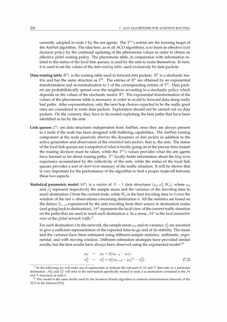
206 7. ACO ALGORITHMS FOR ADAPTIVE ROUTING
currently adopted at node k by the ant agents. The T k’s entries are the learning target of
the AntNet algorithm. The idea here, as in all ACO algorithms, is to learn an effective local
decision policy by the continual updating of the pheromone values in order to obtain an
effective global routing policy. The pheromone table, in conjunction with information re-
lated to the status of the local link queues, is used by the ants to route themselves. In turn,
it is used to set the values of the data-routing table, used exclusively by data packets.
Data-routing tableRk: is the routing table used to forward data packets. Rk is a stochastic ma-
trix and has the same structure as T k. The entries of Rk are obtained by an exponential
transformation and re-normalization to 1 of the corresponding entries of T k. Data pack-
ets are probabilistically spread over the neighbors according to a stochastic policy which
depends on the values of the stochastic matrix Rk. The exponential transformation of the
values of the pheromone table is necessary in order to avoid to forward data along really
bad paths. After exponentiation, only the next hop choices expected to be the really good
ones are considered to route data packets. Exploration should not be carried out on data
packets. On the contrary, they have to be routed exploiting the best paths that have been
identified so far by the ants.
Link queues Lk: are data structures independent from AntNet, since they are always present
in a node if the node has been designed with buffering capabilities. The AntNet routing
component at the node passively observes the dynamics of data packets in addition to the
active generation and observation of the simulated data packets, that is, the ants. The status
of the local link queues are a snapshot of what is locally going on at the precise time instant
the routing decision must be taken, while the T k’s values provides what the ant agents
have learned so far about routing paths. T k locally holds information about the long-term
experience accumulated by the collectivity of the ants, while the status of the local link
queues provides a sort of short-term memory of the traffic situation. It will be shown that
is very important for the performance of the algorithm to find a proper trade-off between
these two aspects.
Statistical parametric modelMk: is a vector of N − 1 data structures (µd, σ2d,Wd), where µd
and σ2d represent respectively the sample mean and the variance of the traveling time to
reach destination d from the current node, whileWd is the best traveling time to d over the
window of the last w observations concerning destination d. All the statistics are based on
the delays Tk→d experienced by the ants traveling from their source to destination nodes
(and going back to destination).Mk represents the local view of the current traffic situation
on the paths that are used to reach each destination d. In a sense,Mk is the local parametric
view of the global network traffic.9
For each destination d in the network, the sample mean µd and its variance σ2d are assumed
to give a sufficient representation of the expected time-to-go and of its stability. The mean
and the variance have been estimated using different sample statistics: arithmetic, expo-
nential, and with moving window. Different estimation strategies have provided similar
results, but the best results have always been observed using the exponential model:10
µd ← µd + η(ok→d − µd),σ2d ← σ2
d + η(
(ok→d − µd)2 − σ2d
)
, (7.2)
9 In the following we will make use of superscripts to indicate the sub-part of M and T that refer to a particulardestination: Mk
dand T k
dwill refer to the information specifically related to node d as destination contained in the M
and T structures of node k.10 This model is the same model used by the Jacobson/Karels algorithm to estimate retransmission timeouts of the
TCP on the Internet [351].
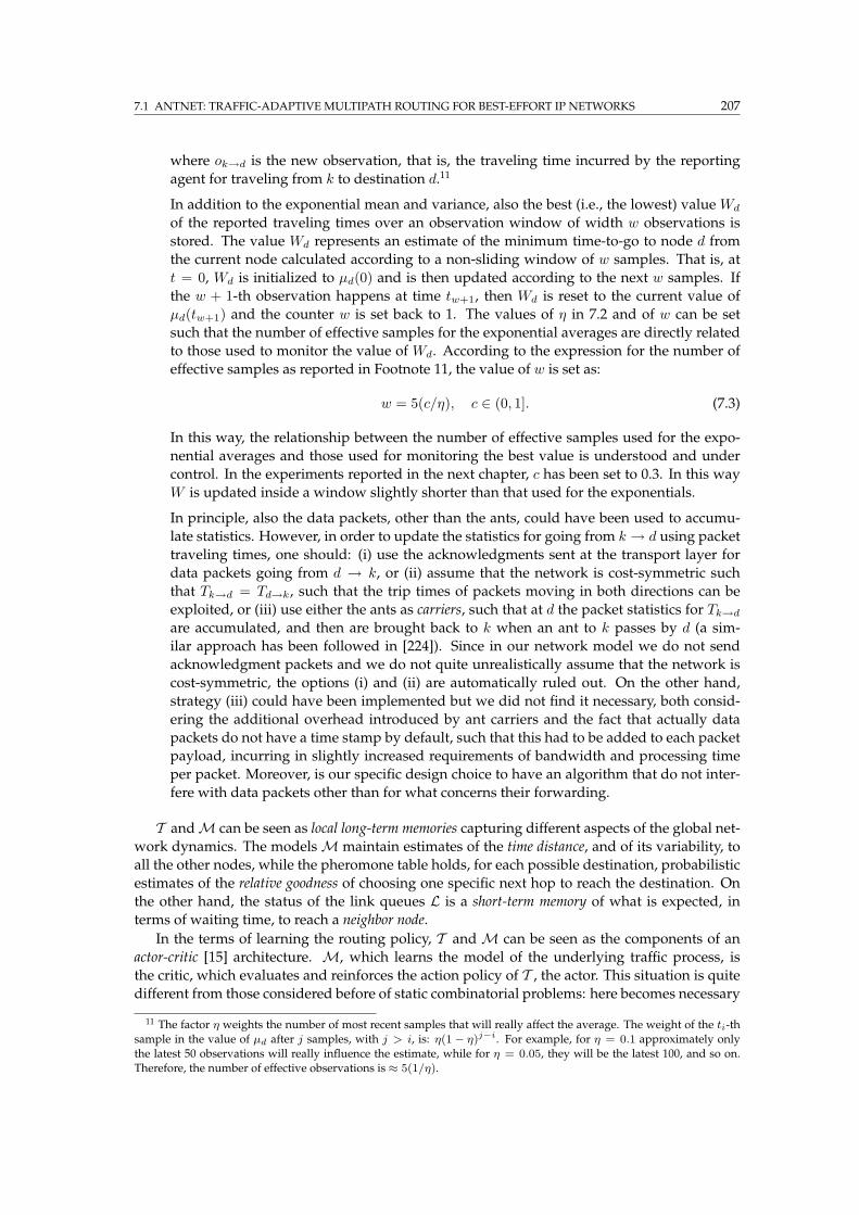
7.1 ANTNET: TRAFFIC-ADAPTIVE MULTIPATH ROUTING FOR BEST-EFFORT IP NETWORKS 207
where ok→d is the new observation, that is, the traveling time incurred by the reporting
agent for traveling from k to destination d.11
In addition to the exponential mean and variance, also the best (i.e., the lowest) valueWd
of the reported traveling times over an observation window of width w observations is
stored. The value Wd represents an estimate of the minimum time-to-go to node d from
the current node calculated according to a non-sliding window of w samples. That is, at
t = 0, Wd is initialized to µd(0) and is then updated according to the next w samples. If
the w + 1-th observation happens at time tw+1, then Wd is reset to the current value of
µd(tw+1) and the counter w is set back to 1. The values of η in 7.2 and of w can be set
such that the number of effective samples for the exponential averages are directly related
to those used to monitor the value of Wd. According to the expression for the number of
effective samples as reported in Footnote 11, the value of w is set as:
w = 5(c/η), c ∈ (0, 1]. (7.3)
In this way, the relationship between the number of effective samples used for the expo-
nential averages and those used for monitoring the best value is understood and under
control. In the experiments reported in the next chapter, c has been set to 0.3. In this way
W is updated inside a window slightly shorter than that used for the exponentials.
In principle, also the data packets, other than the ants, could have been used to accumu-
late statistics. However, in order to update the statistics for going from k → d using packet
traveling times, one should: (i) use the acknowledgments sent at the transport layer for
data packets going from d → k, or (ii) assume that the network is cost-symmetric such
that Tk→d = Td→k, such that the trip times of packets moving in both directions can be
exploited, or (iii) use either the ants as carriers, such that at d the packet statistics for Tk→d
are accumulated, and then are brought back to k when an ant to k passes by d (a sim-
ilar approach has been followed in [224]). Since in our network model we do not send
acknowledgment packets and we do not quite unrealistically assume that the network is
cost-symmetric, the options (i) and (ii) are automatically ruled out. On the other hand,
strategy (iii) could have been implemented but we did not find it necessary, both consid-
ering the additional overhead introduced by ant carriers and the fact that actually data
packets do not have a time stamp by default, such that this had to be added to each packet
payload, incurring in slightly increased requirements of bandwidth and processing time
per packet. Moreover, is our specific design choice to have an algorithm that do not inter-
fere with data packets other than for what concerns their forwarding.
T andM can be seen as local long-term memories capturing different aspects of the global net-
work dynamics. The modelsM maintain estimates of the time distance, and of its variability, to
all the other nodes, while the pheromone table holds, for each possible destination, probabilistic
estimates of the relative goodness of choosing one specific next hop to reach the destination. On
the other hand, the status of the link queues L is a short-term memory of what is expected, in
terms of waiting time, to reach a neighbor node.
In the terms of learning the routing policy, T andM can be seen as the components of an
actor-critic [15] architecture. M, which learns the model of the underlying traffic process, is
the critic, which evaluates and reinforces the action policy of T , the actor. This situation is quite
different from those considered before of static combinatorial problems: here becomes necessary
11 The factor η weights the number of most recent samples that will really affect the average. The weight of the ti-thsample in the value of µd after j samples, with j > i, is: η(1 − η)j−i. For example, for η = 0.1 approximately onlythe latest 50 observations will really influence the estimate, while for η = 0.05, they will be the latest 100, and so on.Therefore, the number of effective observations is ≈ 5(1/η).
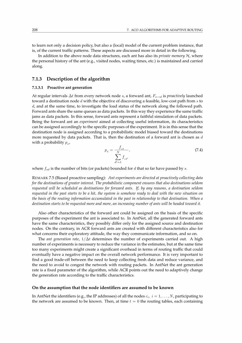
208 7. ACO ALGORITHMS FOR ADAPTIVE ROUTING
to learn not only a decision policy, but also a (local) model of the current problem instance, that
is, of the current traffic patterns. These aspects are discussed more in detail in the following.
In addition to the above node data structures, each ant has also its private memory H, where
the personal history of the ant (e.g., visited nodes, waiting times, etc.) is maintained and carried
along.
7.1.3 Description of the algorithm
7.1.3.1 Proactive ant generation
At regular intervals ∆t from every network node s, a forward ant, Fs→d is proactively launched
toward a destination node dwith the objective of discovering a feasible, low-cost path from s to
d, and at the same time, to investigate the load status of the network along the followed path.
Forward ants share the same queues as data packets. In this way they experience the same traffic
jams as data packets. In this sense, forward ants represent a faithful simulation of data packets.
Being the forward ant an experiment aimed at collecting useful information, its characteristics
can be assigned accordingly to the specific purposes of the experiment. It is in this sense that the
destination node is assigned according to a probabilistic model biased toward the destinations
more requested by data packets. That is, then the destination of a forward ant is chosen as d
with a probability pd,
pd
=f
sd
N∑
d′=1
fsd′
, (7.4)
where fsd is the number of bits (or packets) bounded for d that so far have passed by s.
REMARK 7.5 (Biased proactive sampling): Ant experiments are directed at proactively collecting data
for the destinations of greater interest. The probabilistic component ensures that also destinations seldom
requested will be scheduled as destinations for forward ants. If, by any reasons, a destination seldom
requested in the past starts to be a hit, the system is somehow ready to deal with the new situation on
the basis of the routing information accumulated in the past in relationship to that destination. When a
destination starts to be requested more and more, an increasing number of ants will be headed toward it.
Also other characteristics of the forward ant could be assigned on the basis of the specific
purposes of the experiment the ant is associated to. In AntNet, all the generated forward ants
have the same characteristics, they possibly differ only for the assigned source and destination
nodes. On the contrary, in ACR forward ants are created with different characteristics also for
what concerns their exploratory attitude, the way they communicate information, and so on.
The ant generation rate, 1/∆t determines the number of experiments carried out. A high
number of experiments is necessary to reduce the variance in the estimates, but at the same time
too many experiments might create a significant overhead in terms of routing traffic that could
eventually have a negative impact on the overall network performance. It is very important to
find a good trade-off between the need to keep collecting fresh data and reduce variance, and
the need to avoid to congest the network with routing packets. In AntNet the ant generation
rate is a fixed parameter of the algorithm, while ACR points out the need to adaptively change
the generation rate according to the traffic characteristics.
On the assumption that the node identifiers are assumed to be known
In AntNet the identifiers (e.g., the IP addresses) of all the nodes ci, i = 1, . . . , N , participating to
the network are assumed to be known. Then, at time t = 0 the routing tables, each containing
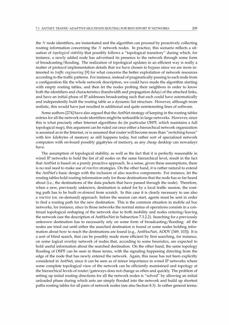
7.1 ANTNET: TRAFFIC-ADAPTIVE MULTIPATH ROUTING FOR BEST-EFFORT IP NETWORKS 209
the N node identifiers, are instantiated and the algorithm can proceed by proactively collecting
routing information concerning the N network nodes. In practice, this scenario reflects a sit-
uation of topological stability that possibly follows a “topological transitory” during which, for
instance, a newly added node has advertised its presence to the network through some form
of broadcasting/flooding. The realization of topological updates in an efficient way is really a
matter of protocol implementation details that we have chosen to bypass since we are more in-
terested in traffic engineering [9] for what concerns the better exploitation of network resources
according to the traffic patterns. For instance, instead of pragmatically passing to each node from
a configuration file the whole network description, we could have made the algorithm starting
with empty routing tables, and then let the nodes probing their neighbors in order to know
both the identifiers and characteristics (bandwidth and propagation delay) of the attached links,
and have an initial phase of IP addresses broadcasting such that each could have automatically
and independently built the routing table as a dynamic list structure. However, although more
realistic, this would have just resulted in additional and quite uninteresting lines of software.
Some authors [274] have also argued that the AntNet strategy of keeping in the routing tables
entries for all the network node identifiersmight be unfeasible in large networks. However, since
this is what precisely other Internet algorithms do (in particular OSPF, which maintains a full
topological map), this argument can be ruled out once either a hierarchical network organization
is assumed as in the Internet, or is assumed that router will becomemore than “switching boxes”
with few kilobytes of memory as still happens today, but rather sort of specialized network
computers with on-board possibly gigabytes of memory, as any cheap desktop can nowadays
have.
The assumption of topological stability, as well as the fact that it is perfectly reasonable in
wired IP networks to hold the list of all nodes on the same hierarchical level, result in the fact
that AntNet is based on a purely proactive approach. In a sense, given these assumptions, there
is no real need to make use of reactive strategies. On the other hand, it is rather natural to extend
the AntNet’s basic design with the inclusion of also reactive components. For instance, let the
routing tables hold routing information only for those destinations that the node has so far heard
about (i.e., the destinations of the data packets that have passed through the node). Therefore,
when a new, previously unknown, destination is asked for by a local traffic session, the rout-
ing path has to be built on-demand from scratch. In this case it is clearly necessary to use also
a reactive (or, on-demand) approach: before the session can start, agents must be sent in order
to find a routing path for the new destination. This is the common situation in mobile ad hoc
networks, for instance, since in those networks the normal status of operations consists in a con-
tinual topological reshaping of the network due to both mobility and nodes entering/leaving
the network (see the description of AntHocNet in Subsection 7.3.2.2). Searching for a previously
unknown destination has to necessarily rely on some form of broadcasting/flooding: all the
nodes are tried out until either the searched destination is found or some nodes holding infor-
mation about how to reach the destinations are found (e.g., AntHocNet, AODV [349, 103]). It is
a sort of blind search, that can be possibly made more efficient by first searching, for instance,
on some logical overlay network of nodes that, according to some heuristics, are expected to
hold useful information about the searched destination. On the other hand, the same topology
flooding of OSPF can be seen in these terms, with the signaling happening directing from the
edge of the node that has newly entered the network. Again, this issue has not been explicitly
considered in AntNet, since it can be seen as of minor importance in wired IP networks where
some complete topological view of the network can be efficiently maintained and topology at
the hierarchical levels of router/gateways does not change so often and quickly. The problem of
setting up initial routing directions for all the network nodes is “solved” by allowing an initial
unloaded phase during which ants are simply flooded into the network and build up shortest
paths routing tables for all pairs of network nodes (see also Section 8.3). In rather general terms:
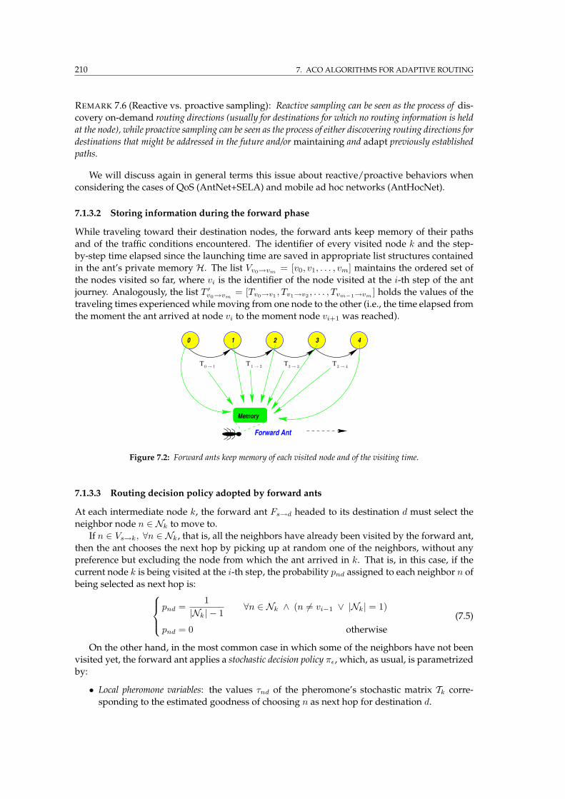
210 7. ACO ALGORITHMS FOR ADAPTIVE ROUTING
REMARK 7.6 (Reactive vs. proactive sampling): Reactive sampling can be seen as the process of dis-
covery on-demand routing directions (usually for destinations for which no routing information is held
at the node), while proactive sampling can be seen as the process of either discovering routing directions for
destinations that might be addressed in the future and/or maintaining and adapt previously established
paths.
We will discuss again in general terms this issue about reactive/proactive behaviors when
considering the cases of QoS (AntNet+SELA) and mobile ad hoc networks (AntHocNet).
7.1.3.2 Storing information during the forward phase
While traveling toward their destination nodes, the forward ants keep memory of their paths
and of the traffic conditions encountered. The identifier of every visited node k and the step-
by-step time elapsed since the launching time are saved in appropriate list structures contained
in the ant’s private memory H. The list Vv0→vm= [v0, v1, . . . , vm] maintains the ordered set of
the nodes visited so far, where vi is the identifier of the node visited at the i-th step of the ant
journey. Analogously, the list T ′v0→vm
= [Tv0→v1 , Tv1→v2 , . . . , Tvm−1→vm] holds the values of the
traveling times experienced while moving from one node to the other (i.e., the time elapsed from
the moment the ant arrived at node vi to the moment node vi+1 was reached).
Forward Ant
Memory
2 40 1 3
T TTT0→ 1 1→ 2 2→ 3 3→ 4
Figure 7.2: Forward ants keep memory of each visited node and of the visiting time.
7.1.3.3 Routing decision policy adopted by forward ants
At each intermediate node k, the forward ant Fs→d headed to its destination d must select the
neighbor node n ∈ Nk to move to.
If n ∈ Vs→k, ∀n ∈ Nk, that is, all the neighbors have already been visited by the forward ant,
then the ant chooses the next hop by picking up at random one of the neighbors, without any
preference but excluding the node from which the ant arrived in k. That is, in this case, if the
current node k is being visited at the i-th step, the probability pnd assigned to each neighbor n of
being selected as next hop is:
pnd =1
|Nk| − 1∀n ∈ Nk ∧ (n 6= vi−1 ∨ |Nk| = 1)
pnd = 0 otherwise
(7.5)
On the other hand, in the most common case in which some of the neighbors have not been
visited yet, the forward ant applies a stochastic decision policy πǫ, which, as usual, is parametrized
by:
• Local pheromone variables: the values τnd of the pheromone’s stochastic matrix Tk corre-
sponding to the estimated goodness of choosing n as next hop for destination d.
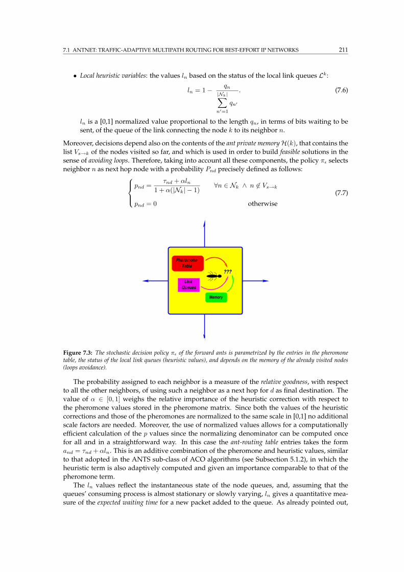
7.1 ANTNET: TRAFFIC-ADAPTIVE MULTIPATH ROUTING FOR BEST-EFFORT IP NETWORKS 211
• Local heuristic variables: the values ln based on the status of the local link queues Lk:
ln = 1− qn|Nk|∑
n′=1
qn′
. (7.6)
ln is a [0,1] normalized value proportional to the length qn, in terms of bits waiting to be
sent, of the queue of the link connecting the node k to its neighbor n.
Moreover, decisions depend also on the contents of the ant private memoryH(k), that contains the
list Vs→k of the nodes visited so far, and which is used in order to build feasible solutions in the
sense of avoiding loops. Therefore, taking into account all these components, the policy πǫ selects
neighbor n as next hop node with a probability Pnd precisely defined as follows:
pnd =τnd + αln
1 + α(|Nk| − 1)∀n ∈ Nk ∧ n 6∈ Vs→k
pnd = 0 otherwise
(7.7)
???
Link
Table
Pheromone
Queues
Memory
Figure 7.3: The stochastic decision policy πǫ of the forward ants is parametrized by the entries in the pheromonetable, the status of the local link queues (heuristic values), and depends on the memory of the already visited nodes(loops avoidance).
The probability assigned to each neighbor is a measure of the relative goodness, with respect
to all the other neighbors, of using such a neighbor as a next hop for d as final destination. The
value of α ∈ [0, 1] weighs the relative importance of the heuristic correction with respect to
the pheromone values stored in the pheromone matrix. Since both the values of the heuristic
corrections and those of the pheromones are normalized to the same scale in [0,1] no additional
scale factors are needed. Moreover, the use of normalized values allows for a computationally
efficient calculation of the p values since the normalizing denominator can be computed once
for all and in a straightforward way. In this case the ant-routing table entries takes the form
and = τnd + αln. This is an additive combination of the pheromone and heuristic values, similar
to that adopted in the ANTS sub-class of ACO algorithms (see Subsection 5.1.2), in which the
heuristic term is also adaptively computed and given an importance comparable to that of the
pheromone term.
The ln values reflect the instantaneous state of the node queues, and, assuming that the
queues’ consuming process is almost stationary or slowly varying, ln gives a quantitative mea-
sure of the expected waiting time for a new packet added to the queue. As already pointed out,
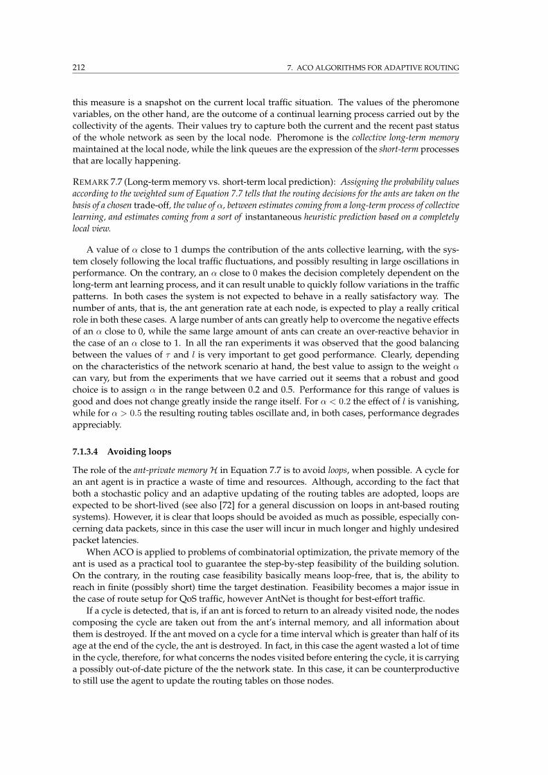
212 7. ACO ALGORITHMS FOR ADAPTIVE ROUTING
this measure is a snapshot on the current local traffic situation. The values of the pheromone
variables, on the other hand, are the outcome of a continual learning process carried out by the
collectivity of the agents. Their values try to capture both the current and the recent past status
of the whole network as seen by the local node. Pheromone is the collective long-term memory
maintained at the local node, while the link queues are the expression of the short-term processes
that are locally happening.
REMARK 7.7 (Long-termmemory vs. short-term local prediction): Assigning the probability values
according to the weighted sum of Equation 7.7 tells that the routing decisions for the ants are taken on the
basis of a chosen trade-off, the value of α, between estimates coming from a long-term process of collective
learning, and estimates coming from a sort of instantaneous heuristic prediction based on a completely
local view.
A value of α close to 1 dumps the contribution of the ants collective learning, with the sys-
tem closely following the local traffic fluctuations, and possibly resulting in large oscillations in
performance. On the contrary, an α close to 0 makes the decision completely dependent on the
long-term ant learning process, and it can result unable to quickly follow variations in the traffic
patterns. In both cases the system is not expected to behave in a really satisfactory way. The
number of ants, that is, the ant generation rate at each node, is expected to play a really critical
role in both these cases. A large number of ants can greatly help to overcome the negative effects
of an α close to 0, while the same large amount of ants can create an over-reactive behavior in
the case of an α close to 1. In all the ran experiments it was observed that the good balancing
between the values of τ and l is very important to get good performance. Clearly, depending
on the characteristics of the network scenario at hand, the best value to assign to the weight α
can vary, but from the experiments that we have carried out it seems that a robust and good
choice is to assign α in the range between 0.2 and 0.5. Performance for this range of values is
good and does not change greatly inside the range itself. For α < 0.2 the effect of l is vanishing,
while for α > 0.5 the resulting routing tables oscillate and, in both cases, performance degrades
appreciably.
7.1.3.4 Avoiding loops
The role of the ant-private memory H in Equation 7.7 is to avoid loops, when possible. A cycle for
an ant agent is in practice a waste of time and resources. Although, according to the fact that
both a stochastic policy and an adaptive updating of the routing tables are adopted, loops are
expected to be short-lived (see also [72] for a general discussion on loops in ant-based routing
systems). However, it is clear that loops should be avoided as much as possible, especially con-
cerning data packets, since in this case the user will incur in much longer and highly undesired
packet latencies.
When ACO is applied to problems of combinatorial optimization, the private memory of the
ant is used as a practical tool to guarantee the step-by-step feasibility of the building solution.
On the contrary, in the routing case feasibility basically means loop-free, that is, the ability to
reach in finite (possibly short) time the target destination. Feasibility becomes a major issue in
the case of route setup for QoS traffic, however AntNet is thought for best-effort traffic.
If a cycle is detected, that is, if an ant is forced to return to an already visited node, the nodes
composing the cycle are taken out from the ant’s internal memory, and all information about
them is destroyed. If the ant moved on a cycle for a time interval which is greater than half of its
age at the end of the cycle, the ant is destroyed. In fact, in this case the agent wasted a lot of time
in the cycle, therefore, for what concerns the nodes visited before entering the cycle, it is carrying
a possibly out-of-date picture of the the network state. In this case, it can be counterproductive
to still use the agent to update the routing tables on those nodes.
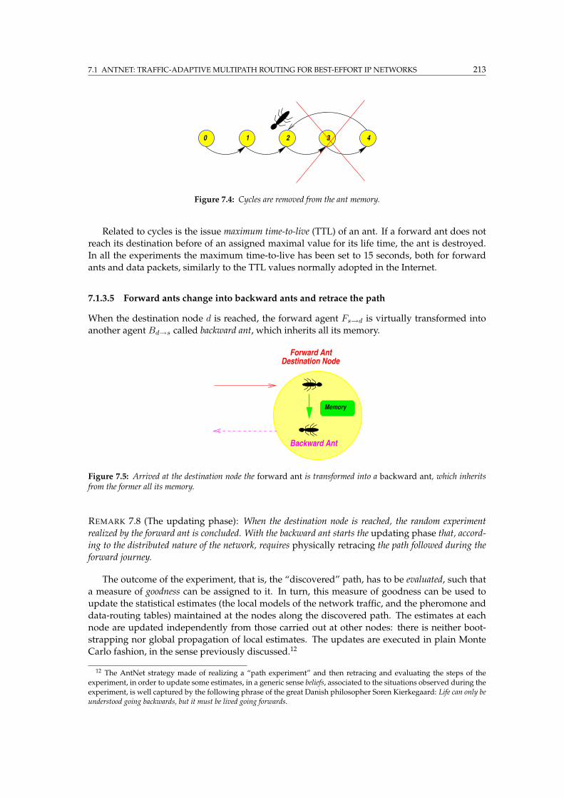
7.1 ANTNET: TRAFFIC-ADAPTIVE MULTIPATH ROUTING FOR BEST-EFFORT IP NETWORKS 213
0 1 2 3 4
Figure 7.4: Cycles are removed from the ant memory.
Related to cycles is the issue maximum time-to-live (TTL) of an ant. If a forward ant does not
reach its destination before of an assigned maximal value for its life time, the ant is destroyed.
In all the experiments the maximum time-to-live has been set to 15 seconds, both for forward
ants and data packets, similarly to the TTL values normally adopted in the Internet.
7.1.3.5 Forward ants change into backward ants and retrace the path
When the destination node d is reached, the forward agent Fs→d is virtually transformed into
another agent Bd→s called backward ant, which inherits all its memory.
Memory
Forward AntDestination Node
Backward Ant
Figure 7.5: Arrived at the destination node the forward ant is transformed into a backward ant, which inheritsfrom the former all its memory.
REMARK 7.8 (The updating phase): When the destination node is reached, the random experiment
realized by the forward ant is concluded. With the backward ant starts the updating phase that, accord-
ing to the distributed nature of the network, requires physically retracing the path followed during the
forward journey.
The outcome of the experiment, that is, the “discovered” path, has to be evaluated, such that
a measure of goodness can be assigned to it. In turn, this measure of goodness can be used to
update the statistical estimates (the local models of the network traffic, and the pheromone and
data-routing tables) maintained at the nodes along the discovered path. The estimates at each
node are updated independently from those carried out at other nodes: there is neither boot-
strapping nor global propagation of local estimates. The updates are executed in plain Monte
Carlo fashion, in the sense previously discussed.12
12 The AntNet strategy made of realizing a “path experiment” and then retracing and evaluating the steps of theexperiment, in order to update some estimates, in a generic sense beliefs, associated to the situations observed during theexperiment, is well captured by the following phrase of the great Danish philosopher Soren Kierkegaard: Life can only beunderstood going backwards, but it must be lived going forwards.
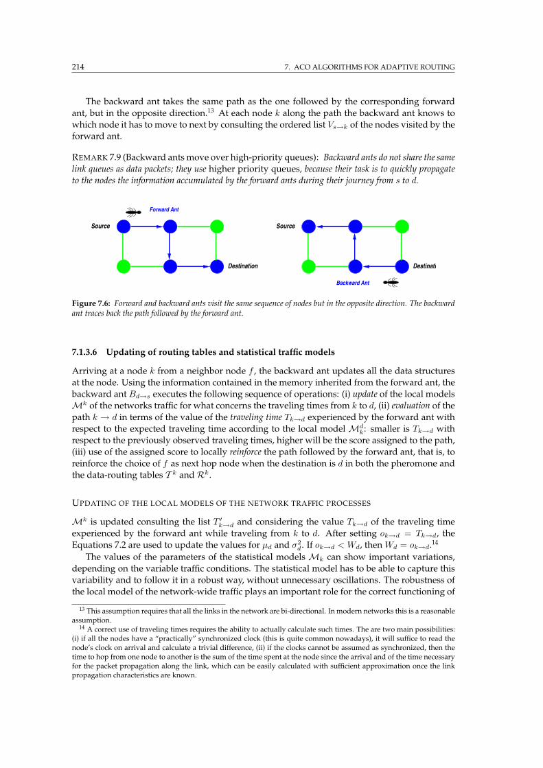
214 7. ACO ALGORITHMS FOR ADAPTIVE ROUTING
The backward ant takes the same path as the one followed by the corresponding forward
ant, but in the opposite direction.13 At each node k along the path the backward ant knows to
which node it has to move to next by consulting the ordered list Vs→k of the nodes visited by the
forward ant.
REMARK 7.9 (Backward ants move over high-priority queues): Backward ants do not share the same
link queues as data packets; they use higher priority queues, because their task is to quickly propagate
to the nodes the information accumulated by the forward ants during their journey from s to d.
Source
Destination
Forward Ant
Source
Destination
Backward Ant
Figure 7.6: Forward and backward ants visit the same sequence of nodes but in the opposite direction. The backwardant traces back the path followed by the forward ant.
7.1.3.6 Updating of routing tables and statistical traffic models
Arriving at a node k from a neighbor node f , the backward ant updates all the data structures
at the node. Using the information contained in the memory inherited from the forward ant, the
backward ant Bd→s executes the following sequence of operations: (i) update of the local models
Mk of the networks traffic for what concerns the traveling times from k to d, (ii) evaluation of the
path k → d in terms of the value of the traveling time Tk→d experienced by the forward ant with
respect to the expected traveling time according to the local modelMdk: smaller is Tk→d with
respect to the previously observed traveling times, higher will be the score assigned to the path,
(iii) use of the assigned score to locally reinforce the path followed by the forward ant, that is, to
reinforce the choice of f as next hop node when the destination is d in both the pheromone and
the data-routing tables T k andRk.
UPDATING OF THE LOCAL MODELS OF THE NETWORK TRAFFIC PROCESSES
Mk is updated consulting the list T ′k→d and considering the value Tk→d of the traveling time
experienced by the forward ant while traveling from k to d. After setting ok→d = Tk→d, the
Equations 7.2 are used to update the values for µd and σ2d. If ok→d < Wd, thenWd = ok→d.
14
The values of the parameters of the statistical modelsMk can show important variations,
depending on the variable traffic conditions. The statistical model has to be able to capture this
variability and to follow it in a robust way, without unnecessary oscillations. The robustness of
the local model of the network-wide traffic plays an important role for the correct functioning of
13 This assumption requires that all the links in the network are bi-directional. In modern networks this is a reasonableassumption.
14 A correct use of traveling times requires the ability to actually calculate such times. The are two main possibilities:(i) if all the nodes have a “practically” synchronized clock (this is quite common nowadays), it will suffice to read thenode’s clock on arrival and calculate a trivial difference, (ii) if the clocks cannot be assumed as synchronized, then thetime to hop from one node to another is the sum of the time spent at the node since the arrival and of the time necessaryfor the packet propagation along the link, which can be easily calculated with sufficient approximation once the linkpropagation characteristics are known.
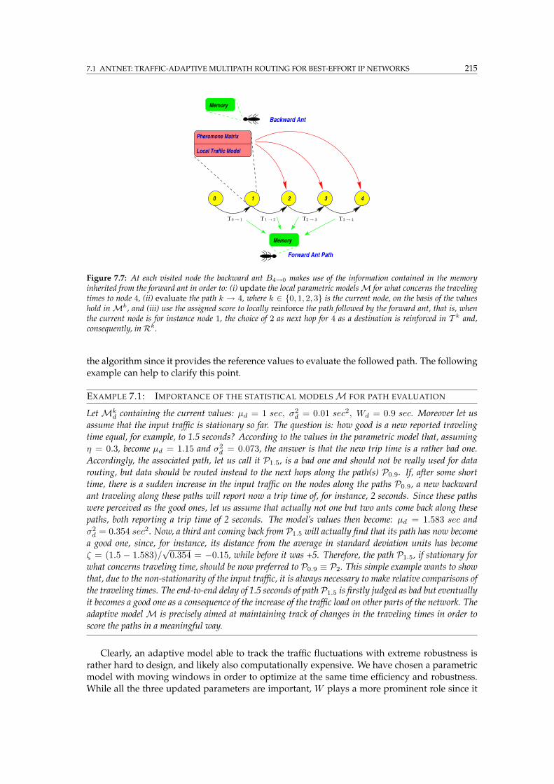
7.1 ANTNET: TRAFFIC-ADAPTIVE MULTIPATH ROUTING FOR BEST-EFFORT IP NETWORKS 215
Forward Ant Path
Backward Ant
Memory
Memory
T T TT
2 40 1 3
Local Traffic Model
Pheromone Matrix
0→ 1 1→ 2 2→ 3 3→ 4
Figure 7.7: At each visited node the backward ant B4→0 makes use of the information contained in the memoryinherited from the forward ant in order to: (i) update the local parametric modelsM for what concerns the travelingtimes to node 4, (ii) evaluate the path k → 4, where k ∈ 0, 1, 2, 3 is the current node, on the basis of the valueshold inMk, and (iii) use the assigned score to locally reinforce the path followed by the forward ant, that is, whenthe current node is for instance node 1, the choice of 2 as next hop for 4 as a destination is reinforced in T k and,consequently, inRk.
the algorithm since it provides the reference values to evaluate the followed path. The following
example can help to clarify this point.
EXAMPLE 7.1: IMPORTANCE OF THE STATISTICAL MODELSM FOR PATH EVALUATION
LetMkd containing the current values: µd = 1 sec, σ2
d = 0.01 sec2, Wd = 0.9 sec. Moreover let us
assume that the input traffic is stationary so far. The question is: how good is a new reported traveling
time equal, for example, to 1.5 seconds? According to the values in the parametric model that, assuming
η = 0.3, become µd = 1.15 and σ2d = 0.073, the answer is that the new trip time is a rather bad one.
Accordingly, the associated path, let us call it P1.5, is a bad one and should not be really used for data
routing, but data should be routed instead to the next hops along the path(s) P0.9. If, after some short
time, there is a sudden increase in the input traffic on the nodes along the paths P0.9, a new backward
ant traveling along these paths will report now a trip time of, for instance, 2 seconds. Since these paths
were perceived as the good ones, let us assume that actually not one but two ants come back along these
paths, both reporting a trip time of 2 seconds. The model’s values then become: µd = 1.583 sec and
σ2d = 0.354 sec2. Now, a third ant coming back from P1.5 will actually find that its path has now become
a good one, since, for instance, its distance from the average in standard deviation units has become
ζ = (1.5 − 1.583)/√
0.354 = −0.15, while before it was +5. Therefore, the path P1.5, if stationary for
what concerns traveling time, should be now preferred to P0.9 ≡ P2. This simple example wants to show
that, due to the non-stationarity of the input traffic, it is always necessary to make relative comparisons of
the traveling times. The end-to-end delay of 1.5 seconds of path P1.5 is firstly judged as bad but eventually
it becomes a good one as a consequence of the increase of the traffic load on other parts of the network. The
adaptive modelM is precisely aimed at maintaining track of changes in the traveling times in order to
score the paths in a meaningful way.
Clearly, an adaptive model able to track the traffic fluctuations with extreme robustness is
rather hard to design, and likely also computationally expensive. We have chosen a parametric
model with moving windows in order to optimize at the same time efficiency and robustness.
While all the three updated parameters are important, W plays a more prominent role since it
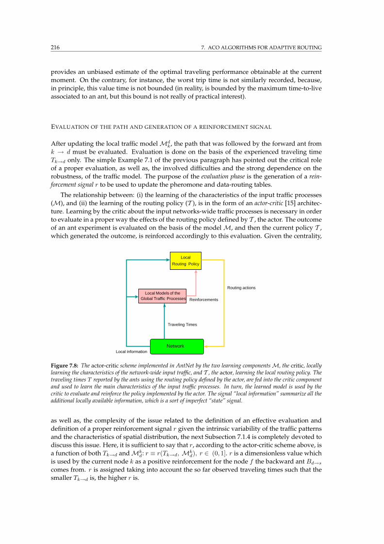
216 7. ACO ALGORITHMS FOR ADAPTIVE ROUTING
provides an unbiased estimate of the optimal traveling performance obtainable at the current
moment. On the contrary, for instance, the worst trip time is not similarly recorded, because,
in principle, this value time is not bounded (in reality, is bounded by the maximum time-to-live
associated to an ant, but this bound is not really of practical interest).
EVALUATION OF THE PATH AND GENERATION OF A REINFORCEMENT SIGNAL
After updating the local traffic modelMdk, the path that was followed by the forward ant from
k → d must be evaluated. Evaluation is done on the basis of the experienced traveling time
Tk→d only. The simple Example 7.1 of the previous paragraph has pointed out the critical role
of a proper evaluation, as well as, the involved difficulties and the strong dependence on the
robustness, of the traffic model. The purpose of the evaluation phase is the generation of a rein-
forcement signal r to be used to update the pheromone and data-routing tables.
The relationship between: (i) the learning of the characteristics of the input traffic processes
(M), and (ii) the learning of the routing policy (T ), is in the form of an actor-critic [15] architec-
ture. Learning by the critic about the input networks-wide traffic processes is necessary in order
to evaluate in a proper way the effects of the routing policy defined by T , the actor. The outcome
of an ant experiment is evaluated on the basis of the modelM, and then the current policy T ,which generated the outcome, is reinforced accordingly to this evaluation. Given the centrality,
Routing
Traveling Times
of theModelsRouting actions
Local information
Local
LocalGlobal Traffic Processes
Policy
Reinforcements
Network
Figure 7.8: The actor-critic scheme implemented in AntNet by the two learning componentsM, the critic, locallylearning the characteristics of the network-wide input traffic, and T , the actor, learning the local routing policy. Thetraveling times T reported by the ants using the routing policy defined by the actor, are fed into the critic componentand used to learn the main characteristics of the input traffic processes. In turn, the learned model is used by thecritic to evaluate and reinforce the policy implemented by the actor. The signal “local information” summarize all theadditional locally available information, which is a sort of imperfect “state” signal.
as well as, the complexity of the issue related to the definition of an effective evaluation and
definition of a proper reinforcement signal r given the intrinsic variability of the traffic patterns
and the characteristics of spatial distribution, the next Subsection 7.1.4 is completely devoted to
discuss this issue. Here, it is sufficient to say that r, according to the actor-critic scheme above, is
a function of both Tk→d andMkd : r ≡ r(Tk→d, Mk
d), r ∈ (0, 1]. r is a dimensionless value which
is used by the current node k as a positive reinforcement for the node f the backward ant Bd→s
comes from. r is assigned taking into account the so far observed traveling times such that the
smaller Tk→d is, the higher r is.
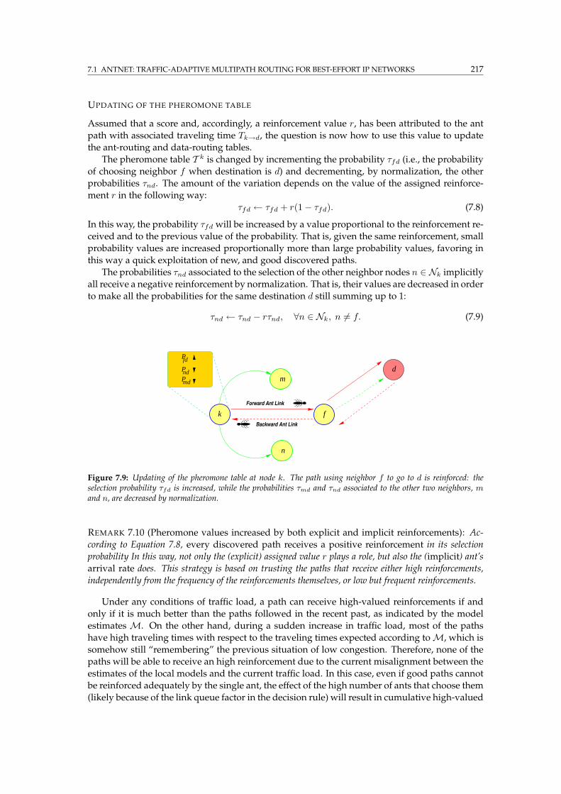
7.1 ANTNET: TRAFFIC-ADAPTIVE MULTIPATH ROUTING FOR BEST-EFFORT IP NETWORKS 217
UPDATING OF THE PHEROMONE TABLE
Assumed that a score and, accordingly, a reinforcement value r, has been attributed to the ant
path with associated traveling time Tk→d, the question is now how to use this value to update
the ant-routing and data-routing tables.
The pheromone table T k is changed by incrementing the probability τfd (i.e., the probability
of choosing neighbor f when destination is d) and decrementing, by normalization, the other
probabilities τnd. The amount of the variation depends on the value of the assigned reinforce-
ment r in the following way:
τfd ← τfd + r(1− τfd). (7.8)
In this way, the probability τfd will be increased by a value proportional to the reinforcement re-
ceived and to the previous value of the probability. That is, given the same reinforcement, small
probability values are increased proportionally more than large probability values, favoring in
this way a quick exploitation of new, and good discovered paths.
The probabilities τnd associated to the selection of the other neighbor nodes n ∈ Nk implicitly
all receive a negative reinforcement by normalization. That is, their values are decreased in order
to make all the probabilities for the same destination d still summing up to 1:
τnd ← τnd − rτnd, ∀n ∈ Nk, n 6= f. (7.9)
Pfd
Pmd
Pnd
f
n
dm
Backward Ant Link
Forward Ant Link
k
Figure 7.9: Updating of the pheromone table at node k. The path using neighbor f to go to d is reinforced: theselection probability τfd is increased, while the probabilities τmd and τnd associated to the other two neighbors, mand n, are decreased by normalization.
REMARK 7.10 (Pheromone values increased by both explicit and implicit reinforcements): Ac-
cording to Equation 7.8, every discovered path receives a positive reinforcement in its selection
probability In this way, not only the (explicit) assigned value r plays a role, but also the (implicit) ant’s
arrival rate does. This strategy is based on trusting the paths that receive either high reinforcements,
independently from the frequency of the reinforcements themselves, or low but frequent reinforcements.
Under any conditions of traffic load, a path can receive high-valued reinforcements if and
only if it is much better than the paths followed in the recent past, as indicated by the model
estimatesM. On the other hand, during a sudden increase in traffic load, most of the paths
have high traveling times with respect to the traveling times expected according toM, which is
somehow still “remembering” the previous situation of low congestion. Therefore, none of the
paths will be able to receive an high reinforcement due to the current misalignment between the
estimates of the local models and the current traffic load. In this case, even if good paths cannot
be reinforced adequately by the single ant, the effect of the high number of ants that choose them
(likely because of the link queue factor in the decision rule) will result in cumulative high-valued
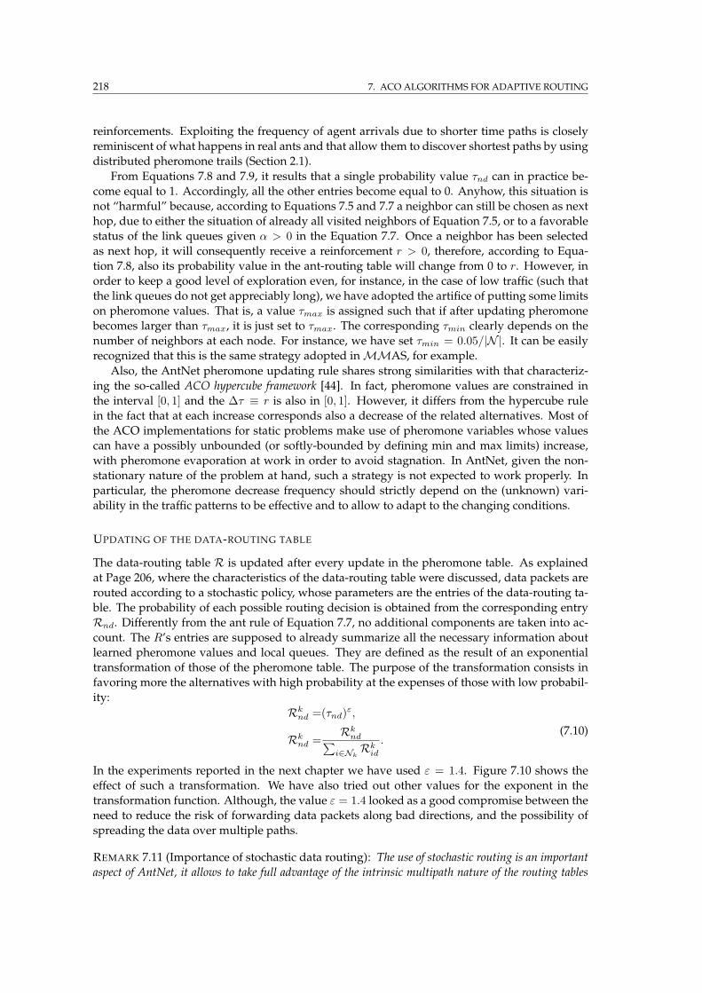
218 7. ACO ALGORITHMS FOR ADAPTIVE ROUTING
reinforcements. Exploiting the frequency of agent arrivals due to shorter time paths is closely
reminiscent of what happens in real ants and that allow them to discover shortest paths by using
distributed pheromone trails (Section 2.1).
From Equations 7.8 and 7.9, it results that a single probability value τnd can in practice be-
come equal to 1. Accordingly, all the other entries become equal to 0. Anyhow, this situation is
not “harmful” because, according to Equations 7.5 and 7.7 a neighbor can still be chosen as next
hop, due to either the situation of already all visited neighbors of Equation 7.5, or to a favorable
status of the link queues given α > 0 in the Equation 7.7. Once a neighbor has been selected
as next hop, it will consequently receive a reinforcement r > 0, therefore, according to Equa-
tion 7.8, also its probability value in the ant-routing table will change from 0 to r. However, in
order to keep a good level of exploration even, for instance, in the case of low traffic (such that
the link queues do not get appreciably long), we have adopted the artifice of putting some limits
on pheromone values. That is, a value τmax is assigned such that if after updating pheromone
becomes larger than τmax, it is just set to τmax. The corresponding τmin clearly depends on the
number of neighbors at each node. For instance, we have set τmin = 0.05/|N |. It can be easily
recognized that this is the same strategy adopted inMMAS, for example.
Also, the AntNet pheromone updating rule shares strong similarities with that characteriz-
ing the so-called ACO hypercube framework [44]. In fact, pheromone values are constrained in
the interval [0, 1] and the ∆τ ≡ r is also in [0, 1]. However, it differs from the hypercube rule
in the fact that at each increase corresponds also a decrease of the related alternatives. Most of
the ACO implementations for static problems make use of pheromone variables whose values
can have a possibly unbounded (or softly-bounded by defining min and max limits) increase,
with pheromone evaporation at work in order to avoid stagnation. In AntNet, given the non-
stationary nature of the problem at hand, such a strategy is not expected to work properly. In
particular, the pheromone decrease frequency should strictly depend on the (unknown) vari-
ability in the traffic patterns to be effective and to allow to adapt to the changing conditions.
UPDATING OF THE DATA-ROUTING TABLE
The data-routing table R is updated after every update in the pheromone table. As explained
at Page 206, where the characteristics of the data-routing table were discussed, data packets are
routed according to a stochastic policy, whose parameters are the entries of the data-routing ta-
ble. The probability of each possible routing decision is obtained from the corresponding entry
Rnd. Differently from the ant rule of Equation 7.7, no additional components are taken into ac-
count. The R’s entries are supposed to already summarize all the necessary information about
learned pheromone values and local queues. They are defined as the result of an exponential
transformation of those of the pheromone table. The purpose of the transformation consists in
favoring more the alternatives with high probability at the expenses of those with low probabil-
ity:
Rknd =(τnd)ε,
Rknd =Rknd
∑
i∈NkRkid
.(7.10)
In the experiments reported in the next chapter we have used ε = 1.4. Figure 7.10 shows the
effect of such a transformation. We have also tried out other values for the exponent in the
transformation function. Although, the value ε = 1.4 looked as a good compromise between the
need to reduce the risk of forwarding data packets along bad directions, and the possibility of
spreading the data over multiple paths.
REMARK 7.11 (Importance of stochastic data routing): The use of stochastic routing is an important
aspect of AntNet, it allows to take full advantage of the intrinsic multipath nature of the routing tables
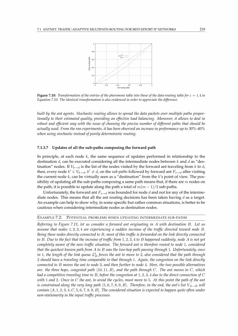
7.1 ANTNET: TRAFFIC-ADAPTIVE MULTIPATH ROUTING FOR BEST-EFFORT IP NETWORKS 219
0
0.2
0.4
0.6
0.8
1
0 0.2 0.4 0.6 0.8 1
Dat
a-ro
utin
g ta
ble
Ant-routing table
y=x1.4
y=x
Figure 7.10: Transformation of the entries of the pheromone table into those of the data-routing table for ε = 1.4 inEquation 7.10. The identical transformation is also evidenced in order to appreciate the difference.
built by the ant agents. Stochastic routing allows to spread the data packets over multiple paths propor-
tionally to their estimated quality, providing an effective load balancing. Moreover, it allows to deal in
robust and efficient way with the issue of choosing the precise number of different paths that should be
actually used. From the ran experiments, it has been observed an increase in performance up to 30%-40%
when using stochastic instead of purely deterministic routing.
7.1.3.7 Updates of all the sub-paths composing the forward path
In principle, at each node k, the same sequence of updates performed in relationship to the
destination d, can be executed considering all the intermediate nodes between k and d as “des-
tination” nodes. If Vk→d is the list of the nodes visited by the forward ant traveling from k to d,
then, every node k′ ∈ Vk→d, k′ 6= d, on the sub-paths followed by forward ant Fs→d after visiting
the current node k, can be virtually seen as a “destination” from the k’s point of view. The pos-
sibility of updating all the sub-paths composing a same path means that, if there arem nodes on
the path, it is possible to update along the path a total ofm(m− 1)/2 sub-paths.
Unfortunately, the forward ant Fs→d was bounded for node d and not for any of the interme-
diate nodes. This means that all the ant routing decisions has been taken having d as a target.
An example can help to show why, in some specific but rather common situations, is better to be
cautious when considering intermediate nodes as destination nodes.
EXAMPLE 7.2: POTENTIAL PROBLEMS WHEN UPDATING INTERMEDIATE SUB-PATHS
Referring to Figure 7.11, let us consider a forward ant originating in A with destination B. Let us
assume that nodes 1, 2, 3, 4 are experiencing a sudden increase of the traffic directed toward node B.
Being these nodes directly connected to B, most of this traffic is forwarded on the link directly connected
to B. Due to the fact that the increase of traffic from 1, 2, 3, 4 to B happened suddenly, node A is not yet
completely aware of the new traffic situation. The forward ant is therefore routed to node 1, considered
that the quickest known path from A to B was the two-hop path passing through 1. Unfortunately, once
in 1, the length of the link queue L1B forces the ant to move to 2, also considered that the path through
2 should have a traveling time comparable to that through 1. Again, the congestion on the link directly
connected to B moves the ant to node 3, and then further to node 4. Here, the two possible alternatives
are: the three hops, congested path 〈10, 11, B〉, and the path through C. The ant moves to C, which
had a competitive traveling time to B, before the congestion at 1, 2, 3, 4 due to the direct connection of C
with 1 and 2. Once in C the ant, to avoid the cycles, must move to 5. At this point the path of the ant
is constrained along the very long path 〈5, 6, 7, 8, 9, B〉. Therefore, in the end, the ant’s list VA→B will
contain [A, 1, 2, 3, 4, C, 5, 6, 7, 8, 9, B]. The considered situation is expected to happen quite often under
non-stationarity in the input traffic processes.
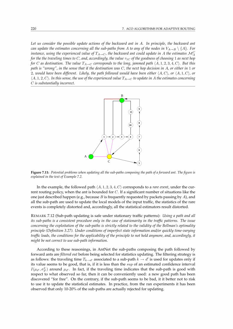
220 7. ACO ALGORITHMS FOR ADAPTIVE ROUTING
Let us consider the possible update actions of the backward ant in A. In principle, the backward ant
can update the estimates concerning all the sub-paths from A to any of the nodes in VA→B \ A. Forinstance, using the experienced value of TA→C , the backward ant could update in A the estimatesMC
A
for the the traveling times to C, and, accordingly, the value τ1C of the goodness of choosing 1 as next hop
for C as destination. The value TA→C corresponds to the long, jammed path 〈A, 1, 2, 3, 4, C〉. But thispath is “wrong”, in the sense that if the destination was C, the next hop decision in A, or either in 1 or
2, would have been different. Likely, the path followed would have been either 〈A,C〉, or 〈A, 1, C〉, or〈A, 1, 2, C〉. In this sense, the use of the experienced value TA→C to update in A the estimates concerning
C is substantially incorrect.
C
A
B
1 2 3 4
8
7
6
5
9
10
11
Figure 7.11: Potential problems when updating all the sub-paths composing the path of a forward ant. The figure isexplained in the text of Example 7.2.
In the example, the followed path 〈A, 1, 2, 3, 4, C〉 corresponds to a rare event, under the cur-
rent routing policy, when the ant is bounded for C. If a significant number of situations like the
one just described happen (e.g., becauseB is frequently requested by packets passing byA), and
all the sub-path are used to update the local models of the input traffic, the statistics of the rare
events is completely distorted and, accordingly, all the statistical estimators result distorted.
REMARK 7.12 (Sub-path updating is safe under stationary traffic patterns): Using a path and all
its sub-paths is a consistent procedure only in the case of stationarity in the traffic patterns. The issue
concerning the exploitation of the sub-paths is strictly related to the validity of the Bellman’s optimality
principle (Definition 3.27). Under conditions of imperfect state information and/or quickly time-varying
traffic loads, the conditions for the applicability of the principle to not hold anymore, and, accordingly, it
might be not correct to use sub-path information.
According to these reasonings, in AntNet the sub-paths composing the path followed by
forward ants are filtered out before being selected for statistics updating. The filtering strategy is
as follows: the traveling time Tk→d′ associated to a sub-path k → d′ is used for updates only if
its value seems to be good, that is, if it is less than the sup of an estimated confidence interval
I(µd′ , σ2d′) around µd′ . In fact, if the traveling time indicates that the sub-path is good with
respect to what observed so far, then it can be conveniently used: a new good path has been
discovered “for free”. On the contrary, if the sub-path seems to be bad, it it better not to risk
to use it to update the statistical estimates. In practice, from the ran experiments it has been
observed that only 10-20% of the sub-paths are actually rejected for updating.
7.1 ANTNET: TRAFFIC-ADAPTIVE MULTIPATH ROUTING FOR BEST-EFFORT IP NETWORKS 221
7.1.3.8 A complete example and pseudo-code description
A complete c-like pseudo-code description of the actions of forward and backward ants is re-
ported in Algorithm 7.1, while an example of the forward-backward behavior of AntNet ants is
illustrated bymeans of Figure 7.12. The forward ant, F1→4, moves along the path 1→ 2→ 3→ 4
and, arrived at node 4, it is transformed in the backward antB4→1 that will travel in the opposite
direction. At each node k, k = 3, 2, 1, the backward ant uses the contents of the lists V1→4(k) and
T ′1→4(k) to update the values forMk(µ4, σ
24 ,W4), and, in case of good sub-paths, to update also
the values forMk(µi, σ2i ,Wi), i = k+ 1, . . . , 3. At the same time, the pheromone table T k is up-
dated by (a) incrementing the goodness τj4, j = k+1, of the node k+1 which is the node the ant
B4→1 came from, for the cases of node i = k+1, . . . , 4 as destination node, and (b) decrementing
by normalization the value of the probabilities for the other neighbors (here not shown). The
increment is a function of the traveling time experienced by the forward ant going from node k
to destination node i. As it happens forM, the pheromone table is also always updated for the
case of node 4 as destination, while the other nodes i′ = k + 1, . . . , 3 on the sub-paths are taken
in consideration as destination nodes only if the traveling time associated to the corresponding
sub-path of the forward ant is good in statistical sense.
( 1 4)
2 41 3
Forward Ant (1 4 )
Backward Ant
Figure 7.12: A complete example, described in the text, of the forward-backward behavior in AntNet.
7.1.4 A critical issue: how to measure the relative goodness of a path?
The traveling time (or end-to-end delay) Tk→d experienced by the forward ant is the metric used
in AntNet to measure the goodness of the followed path Pk→d. Tk→d is a good indicator of the
absolute quality of Pk→d because is a sort of aggregate measure that depends on both physical
characteristics (number of hops, transmission capacity of the used links, processing speed of the
crossed nodes) and traffic conditions (the forward ants share the same queues as data packets).
EXAMPLE 7.3: ALTERNATIVES TO THE USE OF TRAVELING TIME FOR PATH EVALUATION
In principle, other metrics could have been used to score the path (this could be a future issue to explore).
For instance, the number of hops could have been also used. A routing strategy preferentially choosing
the paths with minimal number of hops tends to minimize resources utilization in terms of nodes involved
in routing data traffic for the same source-destination pair. On the other hand, paths with low number of
hops are expected to be more robust to failures and easy to control/monitor.
In AntHocNet we make use, for mobile ad hoc networks, of a composite metric taking into account both
traveling time and number of hops: J(Pk→d) = Tk→d + THHk→d, where TH is the time for one hop
under unloaded conditions, andHk→d is the number of hops in the path. In this way, the number of hops
is conveniently converted to a time. If the time TH cannot be assumed as the same for all links it should
be calculated link by link (and possibly, in this case, the ant trip time should not include the propagation
time, that would be automatically included in the TH values).
The different role between queuing time and propagation time is actually well captured byWedde et al. [443]:
in their bee-inspired algorithm they assign the cost of a link according to a formula that separates the con-
tribution due to propagation time from that due to queuing time. The rationale behind this choice consists
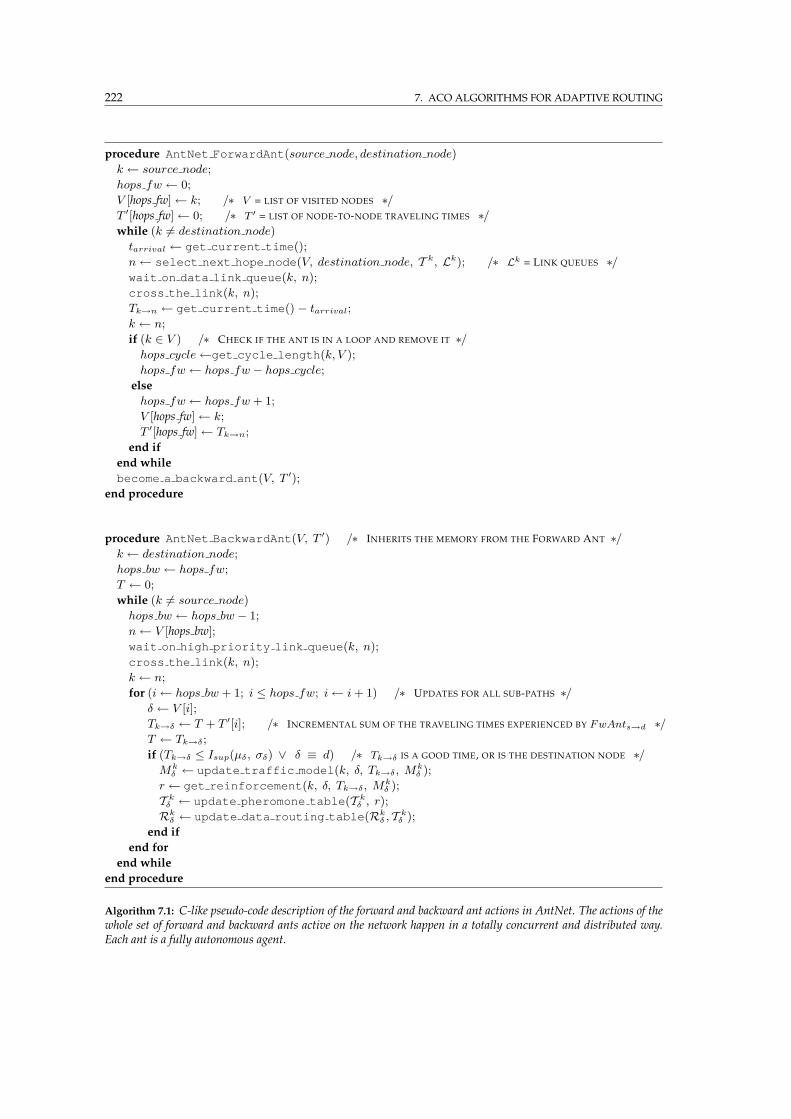
222 7. ACO ALGORITHMS FOR ADAPTIVE ROUTING
procedure AntNet ForwardAnt(source node, destination node)
k ← source node;
hops fw ← 0;
V [hops fw]← k; /∗ V = LIST OF VISITED NODES ∗/
T ′[hops fw]← 0; /∗ T ′ = LIST OF NODE-TO-NODE TRAVELING TIMES ∗/
while (k 6= destination node)
tarrival ← get current time();
n← select next hope node(V, destination node, T k, Lk); /∗ Lk = LINK QUEUES ∗/
wait on data link queue(k, n);
cross the link(k, n);
Tk→n ← get current time() − tarrival;
k ← n;
if (k ∈ V ) /∗ CHECK IF THE ANT IS IN A LOOP AND REMOVE IT ∗/
hops cycle←get cycle length(k, V );
hops fw ← hops fw − hops cycle;
else
hops fw ← hops fw + 1;
V [hops fw]← k;
T ′[hops fw]← Tk→n;
end if
end while
become a backward ant(V, T ′);
end procedure
procedure AntNet BackwardAnt(V, T ′) /∗ INHERITS THE MEMORY FROM THE FORWARD ANT ∗/
k ← destination node;
hops bw ← hops fw;
T ← 0;
while (k 6= source node)
hops bw ← hops bw − 1;
n← V [hops bw];
wait on high priority link queue(k, n);
cross the link(k, n);
k ← n;
for (i← hops bw + 1; i ≤ hops fw; i← i + 1) /∗ UPDATES FOR ALL SUB-PATHS ∗/
δ ← V [i];
Tk→δ ← T + T ′[i]; /∗ INCREMENTAL SUM OF THE TRAVELING TIMES EXPERIENCED BY FwAnts→d ∗/
T ← Tk→δ;
if (Tk→δ ≤ Isup(µδ, σδ) ∨ δ ≡ d) /∗ Tk→δ IS A GOOD TIME, OR IS THE DESTINATION NODE ∗/
Mkδ ← update traffic model(k, δ, Tk→δ, Mk
δ );
r ← get reinforcement(k, δ, Tk→δ, Mkδ );
T kδ ← update pheromone table(T k
δ , r);
Rkδ ← update data routing table(Rk
δ , T kδ );
end if
end for
end while
end procedure
Algorithm 7.1: C-like pseudo-code description of the forward and backward ant actions in AntNet. The actions of thewhole set of forward and backward ants active on the network happen in a totally concurrent and distributed way.Each ant is a fully autonomous agent.
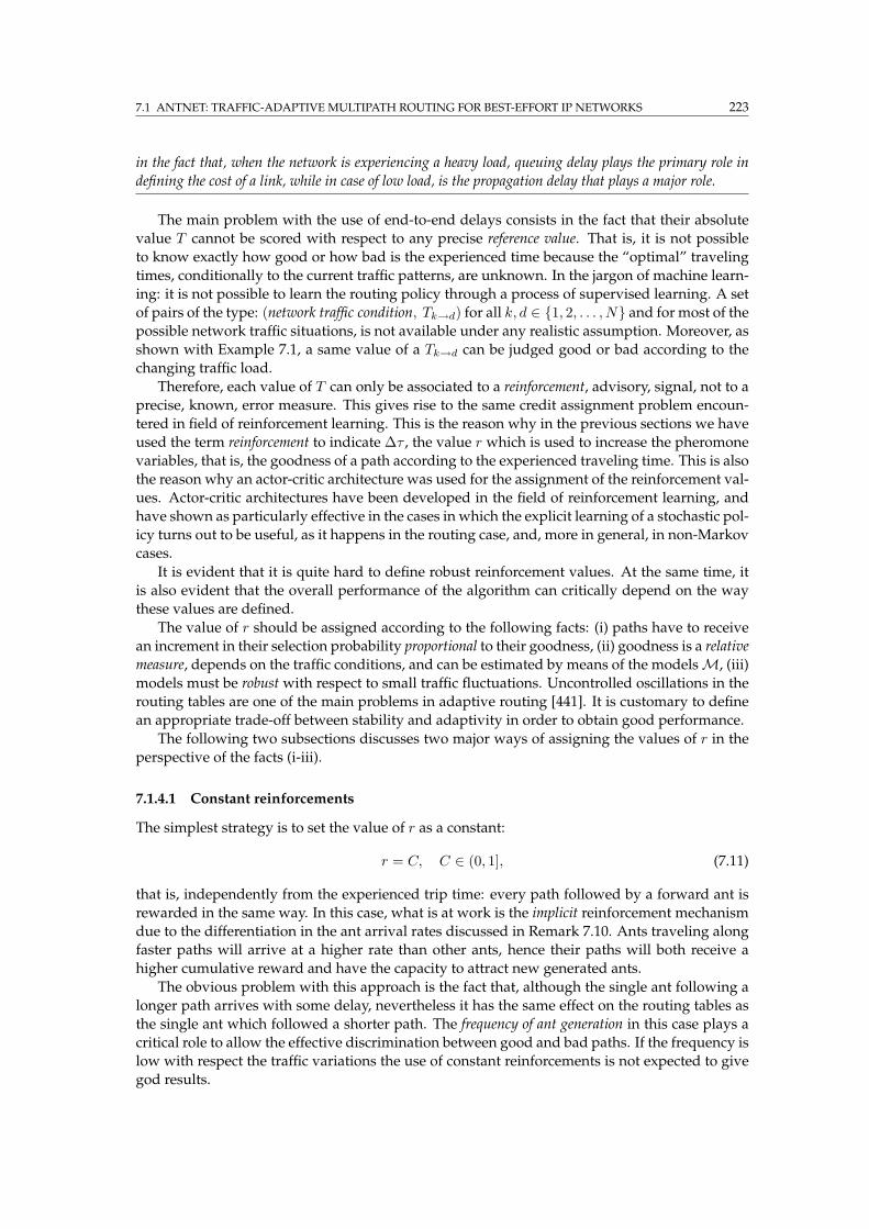
7.1 ANTNET: TRAFFIC-ADAPTIVE MULTIPATH ROUTING FOR BEST-EFFORT IP NETWORKS 223
in the fact that, when the network is experiencing a heavy load, queuing delay plays the primary role in
defining the cost of a link, while in case of low load, is the propagation delay that plays a major role.
The main problem with the use of end-to-end delays consists in the fact that their absolute
value T cannot be scored with respect to any precise reference value. That is, it is not possible
to know exactly how good or how bad is the experienced time because the “optimal” traveling
times, conditionally to the current traffic patterns, are unknown. In the jargon of machine learn-
ing: it is not possible to learn the routing policy through a process of supervised learning. A set
of pairs of the type: (network traffic condition, Tk→d) for all k, d ∈ 1, 2, . . . , N and for most of the
possible network traffic situations, is not available under any realistic assumption. Moreover, as
shown with Example 7.1, a same value of a Tk→d can be judged good or bad according to the
changing traffic load.
Therefore, each value of T can only be associated to a reinforcement, advisory, signal, not to a
precise, known, error measure. This gives rise to the same credit assignment problem encoun-
tered in field of reinforcement learning. This is the reason why in the previous sections we have
used the term reinforcement to indicate ∆τ , the value r which is used to increase the pheromone
variables, that is, the goodness of a path according to the experienced traveling time. This is also
the reason why an actor-critic architecture was used for the assignment of the reinforcement val-
ues. Actor-critic architectures have been developed in the field of reinforcement learning, and
have shown as particularly effective in the cases in which the explicit learning of a stochastic pol-
icy turns out to be useful, as it happens in the routing case, and, more in general, in non-Markov
cases.
It is evident that it is quite hard to define robust reinforcement values. At the same time, it
is also evident that the overall performance of the algorithm can critically depend on the way
these values are defined.
The value of r should be assigned according to the following facts: (i) paths have to receive
an increment in their selection probability proportional to their goodness, (ii) goodness is a relative
measure, depends on the traffic conditions, and can be estimated by means of the modelsM, (iii)
models must be robust with respect to small traffic fluctuations. Uncontrolled oscillations in the
routing tables are one of the main problems in adaptive routing [441]. It is customary to define
an appropriate trade-off between stability and adaptivity in order to obtain good performance.
The following two subsections discusses two major ways of assigning the values of r in the
perspective of the facts (i-iii).
7.1.4.1 Constant reinforcements
The simplest strategy is to set the value of r as a constant:
r = C, C ∈ (0, 1], (7.11)
that is, independently from the experienced trip time: every path followed by a forward ant is
rewarded in the same way. In this case, what is at work is the implicit reinforcement mechanism
due to the differentiation in the ant arrival rates discussed in Remark 7.10. Ants traveling along
faster paths will arrive at a higher rate than other ants, hence their paths will both receive a
higher cumulative reward and have the capacity to attract new generated ants.
The obvious problem with this approach is the fact that, although the single ant following a
longer path arrives with some delay, nevertheless it has the same effect on the routing tables as
the single ant which followed a shorter path. The frequency of ant generation in this case plays a
critical role to allow the effective discrimination between good and bad paths. If the frequency is
low with respect the traffic variations the use of constant reinforcements is not expected to give
god results.
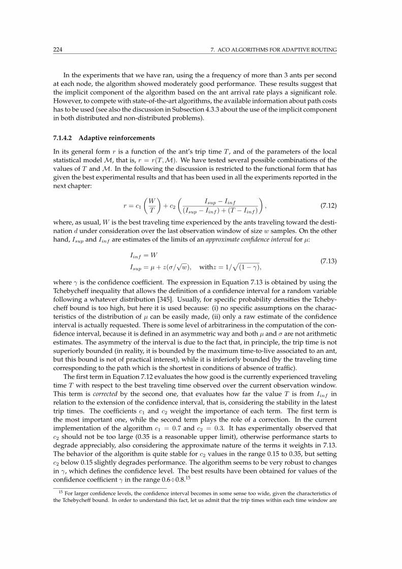
224 7. ACO ALGORITHMS FOR ADAPTIVE ROUTING
In the experiments that we have ran, using the a frequency of more than 3 ants per second
at each node, the algorithm showed moderately good performance. These results suggest that
the implicit component of the algorithm based on the ant arrival rate plays a significant role.
However, to compete with state-of-the-art algorithms, the available information about path costs
has to be used (see also the discussion in Subsection 4.3.3 about the use of the implicit component
in both distributed and non-distributed problems).
7.1.4.2 Adaptive reinforcements
In its general form r is a function of the ant’s trip time T , and of the parameters of the local
statistical modelM, that is, r = r(T,M). We have tested several possible combinations of the
values of T andM. In the following the discussion is restricted to the functional form that has
given the best experimental results and that has been used in all the experiments reported in the
next chapter:
r = c1
(
W
T
)
+ c2
(
Isup − Iinf(Isup − Iinf ) + (T − Iinf )
)
, (7.12)
where, as usual,W is the best traveling time experienced by the ants traveling toward the desti-
nation d under consideration over the last observation window of size w samples. On the other
hand, Isup and Iinf are estimates of the limits of an approximate confidence interval for µ:
Iinf = W
Isup = µ+ z(σ/√w), withz = 1/
√
(1− γ),(7.13)
where γ is the confidence coefficient. The expression in Equation 7.13 is obtained by using the
Tchebycheff inequality that allows the definition of a confidence interval for a random variable
following a whatever distribution [345]. Usually, for specific probability densities the Tcheby-
cheff bound is too high, but here it is used because: (i) no specific assumptions on the charac-
teristics of the distribution of µ can be easily made, (ii) only a raw estimate of the confidence
interval is actually requested. There is some level of arbitrariness in the computation of the con-
fidence interval, because it is defined in an asymmetric way and both µ and σ are not arithmetic
estimates. The asymmetry of the interval is due to the fact that, in principle, the trip time is not
superiorly bounded (in reality, it is bounded by the maximum time-to-live associated to an ant,
but this bound is not of practical interest), while it is inferiorly bounded (by the traveling time
corresponding to the path which is the shortest in conditions of absence of traffic).
The first term in Equation 7.12 evaluates the how good is the currently experienced traveling
time T with respect to the best traveling time observed over the current observation window.
This term is corrected by the second one, that evaluates how far the value T is from Iinf in
relation to the extension of the confidence interval, that is, considering the stability in the latest
trip times. The coefficients c1 and c2 weight the importance of each term. The first term is
the most important one, while the second term plays the role of a correction. In the current
implementation of the algorithm c1 = 0.7 and c2 = 0.3. It has experimentally observed that
c2 should not be too large (0.35 is a reasonable upper limit), otherwise performance starts to
degrade appreciably, also considering the approximate nature of the terms it weights in 7.13.
The behavior of the algorithm is quite stable for c2 values in the range 0.15 to 0.35, but setting
c2 below 0.15 slightly degrades performance. The algorithm seems to be very robust to changes
in γ, which defines the confidence level. The best results have been obtained for values of the
confidence coefficient γ in the range 0.6÷0.8.15
15 For larger confidence levels, the confidence interval becomes in some sense too wide, given the characteristics ofthe Tchebycheff bound. In order to understand this fact, let us admit that the trip times within each time window are
7.1 ANTNET: TRAFFIC-ADAPTIVE MULTIPATH ROUTING FOR BEST-EFFORT IP NETWORKS 225
The denominator of the second term in Equation 7.12 can become equal to zero, in the rather
pathological cases in which Isup = Iinf = T and T = 2Iinf − Isup. In these cases the term
weighted by c2 is simply not taken into account.
In order to prevent the pheromone values going to 1, or to make too large jumps, r is actually
saturated at the value 0.9. Finally, the value of r is squashed by means of a function s(x):
s(x) =
(
1 + exp
(
a
x|Nk|
)
)−1
, x ∈ (0, 1], a ∈ R+, (7.14)
r =s(r)
s(1). (7.15)
By squashing the value of r, the upper scale of the r values is expanded, such that the sen-
sitivity of the system in the case of good (high) values of r is increased. On the contrary, the
lower scale is compressed, bad (near to 0) r values are saturated around 0. In such a way more
emphasis is put on good results. The coefficient a/|Nk| determines a parametric dependence of
0
0.2
0.4
0.6
0.8
1
0 0.2 0.4 0.6 0.8 1
s(r)
/s(1
)
r
5 neighbors4 neighbors3 neighbors2 neighbors
Figure 7.13: Squash functions with a different a/|Nk|.
the squashed reinforcement value on the number |Nk| of neighbors of the node k: the greater thenumber of neighbors, the higher the reinforcement (see Figure 7.13). The rationale behind this
choice is the need to have similar effects independently of the number of neighbor nodes. The
number of neighbors has, in fact, an effect at themoment of the normalization of the probabilistic
entries of the routing table. A more uniform distribution of the probability values is expected,
in general, with an higher number of neighbors, due to the fact that several alternative paths
might result similar. To contrast this tendency, the coefficient a/|Nk| tries to slightly amplify the
possible differences.
REMARK 7.13 (Robustness to parameter setting): In spite of the fact that many parameters are in-
volved, the algorithm has experimentally proved to be very robust to parameter settings. All the different
experiments presented in the next chapter have been realized using the same set of values for the parame-
ters, in spite of the significant differences among the different problem scenarios. Clearly, the performance
could have been improved by mean of a fine tuning of the parameters, choosing different values for the
different problem instances. This tuning process has purposely not been carried out. The target was, in
fact, the design of an algorithm able to show a robust behavior under a variety of completely different
normally distributed. In this case, an expression for the confidence interval similar to the Tchebycheff one, but moreprecise and with a slightly different meaning for the term z, can be written. In particular, setting up a confidence levelof 0.95 implies z ≈ 2. The same value of z for the more general, non Gaussian, case expressed by the Tchebycheffinequality, implies a confidence level of the 65%, which is also the same used in the experiments reported in Chapter 8.
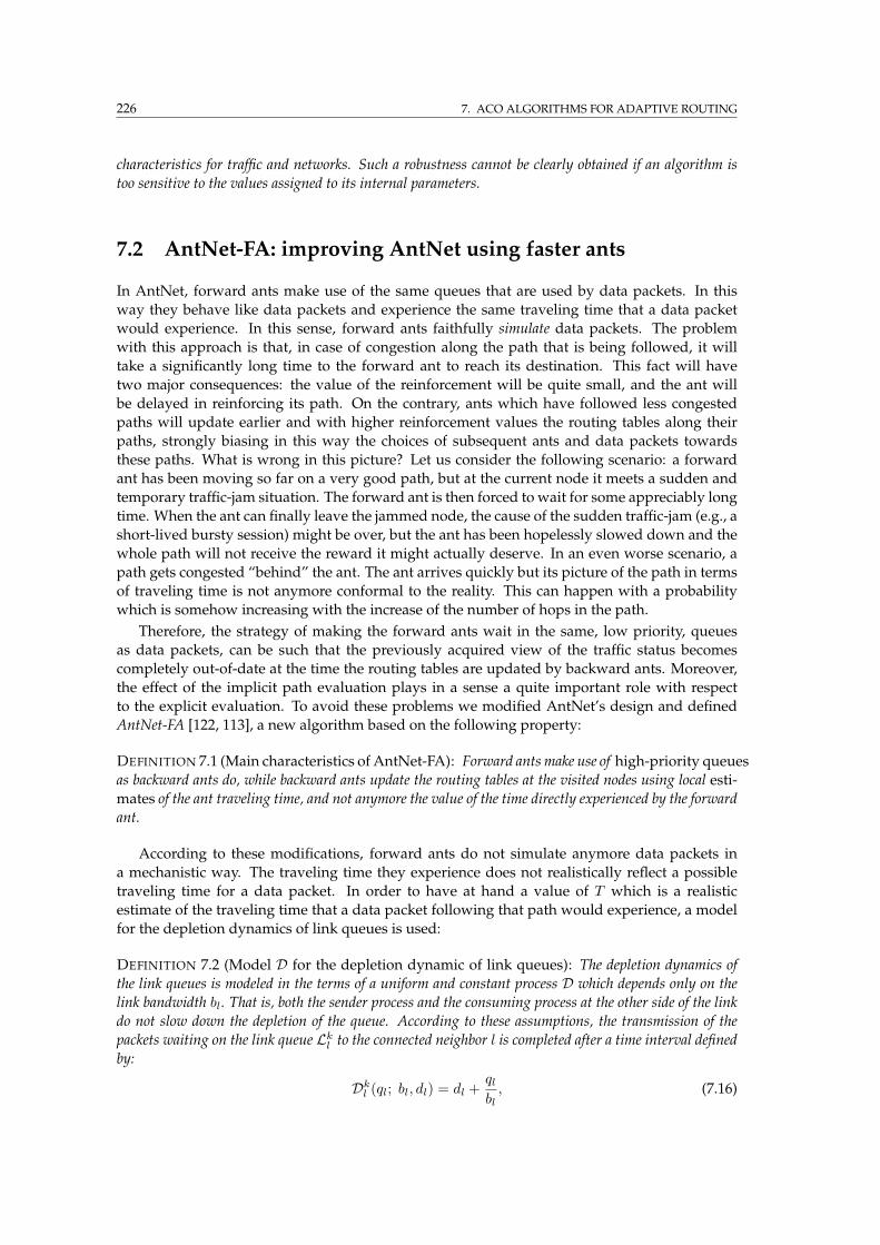
226 7. ACO ALGORITHMS FOR ADAPTIVE ROUTING
characteristics for traffic and networks. Such a robustness cannot be clearly obtained if an algorithm is
too sensitive to the values assigned to its internal parameters.
7.2 AntNet-FA: improving AntNet using faster ants
In AntNet, forward ants make use of the same queues that are used by data packets. In this
way they behave like data packets and experience the same traveling time that a data packet
would experience. In this sense, forward ants faithfully simulate data packets. The problem
with this approach is that, in case of congestion along the path that is being followed, it will
take a significantly long time to the forward ant to reach its destination. This fact will have
two major consequences: the value of the reinforcement will be quite small, and the ant will
be delayed in reinforcing its path. On the contrary, ants which have followed less congested
paths will update earlier and with higher reinforcement values the routing tables along their
paths, strongly biasing in this way the choices of subsequent ants and data packets towards
these paths. What is wrong in this picture? Let us consider the following scenario: a forward
ant has been moving so far on a very good path, but at the current node it meets a sudden and
temporary traffic-jam situation. The forward ant is then forced to wait for some appreciably long
time. When the ant can finally leave the jammed node, the cause of the sudden traffic-jam (e.g., a
short-lived bursty session) might be over, but the ant has been hopelessly slowed down and the
whole path will not receive the reward it might actually deserve. In an even worse scenario, a
path gets congested “behind” the ant. The ant arrives quickly but its picture of the path in terms
of traveling time is not anymore conformal to the reality. This can happen with a probability
which is somehow increasing with the increase of the number of hops in the path.
Therefore, the strategy of making the forward ants wait in the same, low priority, queues
as data packets, can be such that the previously acquired view of the traffic status becomes
completely out-of-date at the time the routing tables are updated by backward ants. Moreover,
the effect of the implicit path evaluation plays in a sense a quite important role with respect
to the explicit evaluation. To avoid these problems we modified AntNet’s design and defined
AntNet-FA [122, 113], a new algorithm based on the following property:
DEFINITION 7.1 (Main characteristics of AntNet-FA): Forward ants make use of high-priority queues
as backward ants do, while backward ants update the routing tables at the visited nodes using local esti-
mates of the ant traveling time, and not anymore the value of the time directly experienced by the forward
ant.
According to these modifications, forward ants do not simulate anymore data packets in
a mechanistic way. The traveling time they experience does not realistically reflect a possible
traveling time for a data packet. In order to have at hand a value of T which is a realistic
estimate of the traveling time that a data packet following that path would experience, a model
for the depletion dynamics of link queues is used:
DEFINITION 7.2 (Model D for the depletion dynamic of link queues): The depletion dynamics of
the link queues is modeled in the terms of a uniform and constant process D which depends only on the
link bandwidth bl. That is, both the sender process and the consuming process at the other side of the link
do not slow down the depletion of the queue. According to these assumptions, the transmission of the
packets waiting on the link queue Lkl to the connected neighbor l is completed after a time interval defined
by:
Dkl (ql; bl, dl) = dl +qlbl, (7.16)
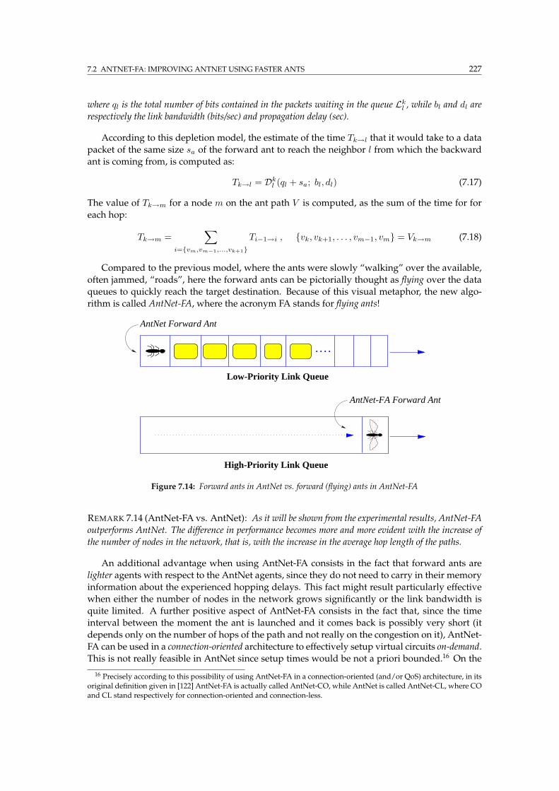
7.2 ANTNET-FA: IMPROVING ANTNET USING FASTER ANTS 227
where ql is the total number of bits contained in the packets waiting in the queue Lkl , while bl and dl arerespectively the link bandwidth (bits/sec) and propagation delay (sec).
According to this depletion model, the estimate of the time Tk→l that it would take to a data
packet of the same size sa of the forward ant to reach the neighbor l from which the backward
ant is coming from, is computed as:
Tk→l = Dkl (ql + sa; bl, dl) (7.17)
The value of Tk→m for a node m on the ant path V is computed, as the sum of the time for for
each hop:
Tk→m =∑
i=vm,vm−1,...,vk+1
Ti−1→i , vk, vk+1, . . . , vm−1, vm = Vk→m (7.18)
Compared to the previous model, where the ants were slowly “walking” over the available,
often jammed, “roads”, here the forward ants can be pictorially thought as flying over the data
queues to quickly reach the target destination. Because of this visual metaphor, the new algo-
rithm is called AntNet-FA, where the acronym FA stands for flying ants!
AntNet-FA Forward Ant
High-Priority Link Queue
. . . .
Low-Priority Link Queue
AntNet Forward Ant
Figure 7.14: Forward ants in AntNet vs. forward (flying) ants in AntNet-FA
REMARK 7.14 (AntNet-FA vs. AntNet): As it will be shown from the experimental results, AntNet-FA
outperforms AntNet. The difference in performance becomes more and more evident with the increase of
the number of nodes in the network, that is, with the increase in the average hop length of the paths.
An additional advantage when using AntNet-FA consists in the fact that forward ants are
lighter agents with respect to the AntNet agents, since they do not need to carry in their memory
information about the experienced hopping delays. This fact might result particularly effective
when either the number of nodes in the network grows significantly or the link bandwidth is
quite limited. A further positive aspect of AntNet-FA consists in the fact that, since the time
interval between the moment the ant is launched and it comes back is possibly very short (it
depends only on the number of hops of the path and not really on the congestion on it), AntNet-
FA can be used in a connection-oriented architecture to effectively setup virtual circuits on-demand.
This is not really feasible in AntNet since setup times would be not a priori bounded.16 On the
16 Precisely according to this possibility of using AntNet-FA in a connection-oriented (and/or QoS) architecture, in itsoriginal definition given in [122] AntNet-FA is actually called AntNet-CO, while AntNet is called AntNet-CL, where COand CL stand respectively for connection-oriented and connection-less.
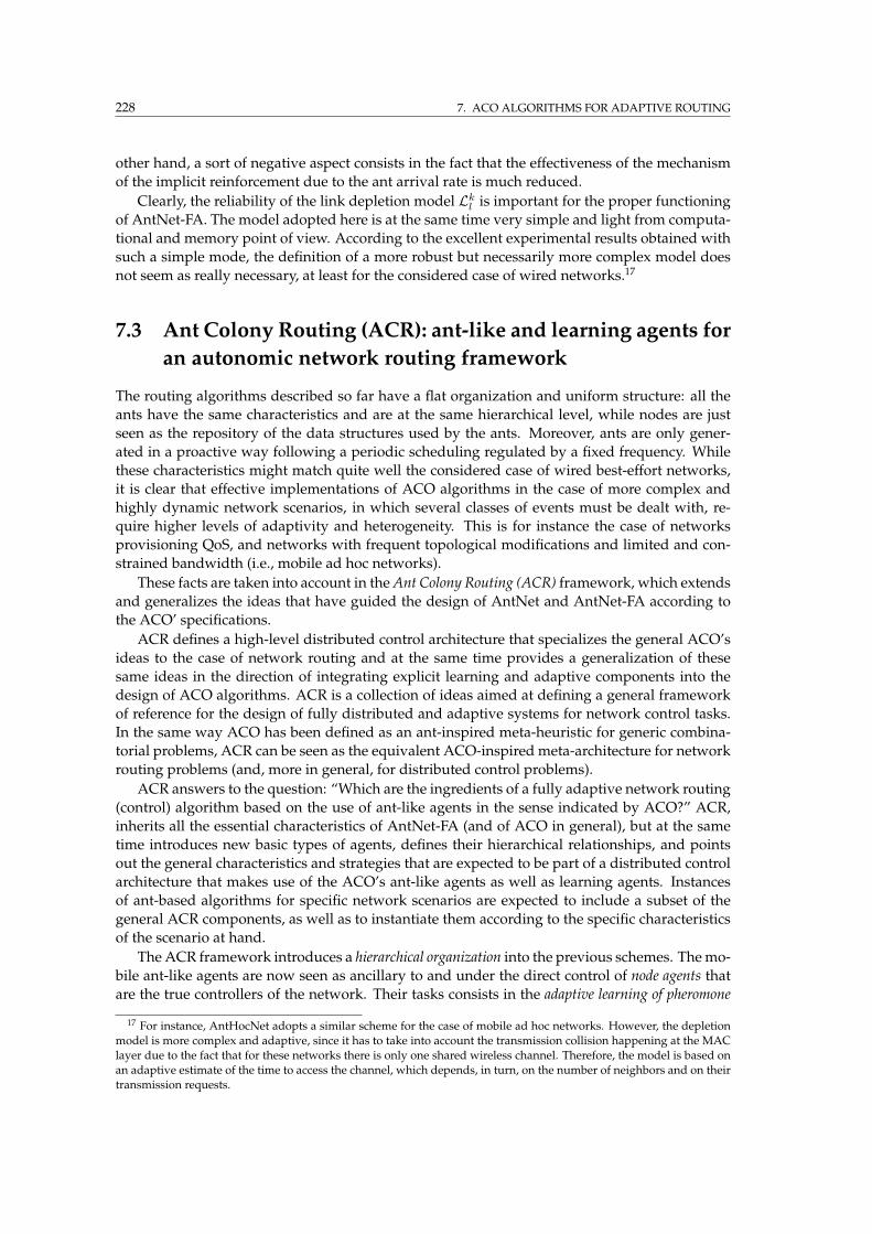
228 7. ACO ALGORITHMS FOR ADAPTIVE ROUTING
other hand, a sort of negative aspect consists in the fact that the effectiveness of the mechanism
of the implicit reinforcement due to the ant arrival rate is much reduced.
Clearly, the reliability of the link depletion model Lkl is important for the proper functioning
of AntNet-FA. The model adopted here is at the same time very simple and light from computa-
tional and memory point of view. According to the excellent experimental results obtained with
such a simple mode, the definition of a more robust but necessarily more complex model does
not seem as really necessary, at least for the considered case of wired networks.17
7.3 Ant Colony Routing (ACR): ant-like and learning agents for
an autonomic network routing framework
The routing algorithms described so far have a flat organization and uniform structure: all the
ants have the same characteristics and are at the same hierarchical level, while nodes are just
seen as the repository of the data structures used by the ants. Moreover, ants are only gener-
ated in a proactive way following a periodic scheduling regulated by a fixed frequency. While
these characteristics might match quite well the considered case of wired best-effort networks,
it is clear that effective implementations of ACO algorithms in the case of more complex and
highly dynamic network scenarios, in which several classes of events must be dealt with, re-
quire higher levels of adaptivity and heterogeneity. This is for instance the case of networks
provisioning QoS, and networks with frequent topological modifications and limited and con-
strained bandwidth (i.e., mobile ad hoc networks).
These facts are taken into account in theAnt Colony Routing (ACR) framework, which extends
and generalizes the ideas that have guided the design of AntNet and AntNet-FA according to
the ACO’ specifications.
ACR defines a high-level distributed control architecture that specializes the general ACO’s
ideas to the case of network routing and at the same time provides a generalization of these
same ideas in the direction of integrating explicit learning and adaptive components into the
design of ACO algorithms. ACR is a collection of ideas aimed at defining a general framework
of reference for the design of fully distributed and adaptive systems for network control tasks.
In the same way ACO has been defined as an ant-inspired meta-heuristic for generic combina-
torial problems, ACR can be seen as the equivalent ACO-inspired meta-architecture for network
routing problems (and, more in general, for distributed control problems).
ACR answers to the question: “Which are the ingredients of a fully adaptive network routing
(control) algorithm based on the use of ant-like agents in the sense indicated by ACO?” ACR,
inherits all the essential characteristics of AntNet-FA (and of ACO in general), but at the same
time introduces new basic types of agents, defines their hierarchical relationships, and points
out the general characteristics and strategies that are expected to be part of a distributed control
architecture that makes use of the ACO’s ant-like agents as well as learning agents. Instances
of ant-based algorithms for specific network scenarios are expected to include a subset of the
general ACR components, as well as to instantiate them according to the specific characteristics
of the scenario at hand.
The ACR framework introduces a hierarchical organization into the previous schemes. Themo-
bile ant-like agents are now seen as ancillary to and under the direct control of node agents that
are the true controllers of the network. Their tasks consists in the adaptive learning of pheromone
17 For instance, AntHocNet adopts a similar scheme for the case of mobile ad hoc networks. However, the depletionmodel is more complex and adaptive, since it has to take into account the transmission collision happening at the MAClayer due to the fact that for these networks there is only one shared wireless channel. Therefore, the model is based onan adaptive estimate of the time to access the channel, which depends, in turn, on the number of neighbors and on theirtransmission requests.
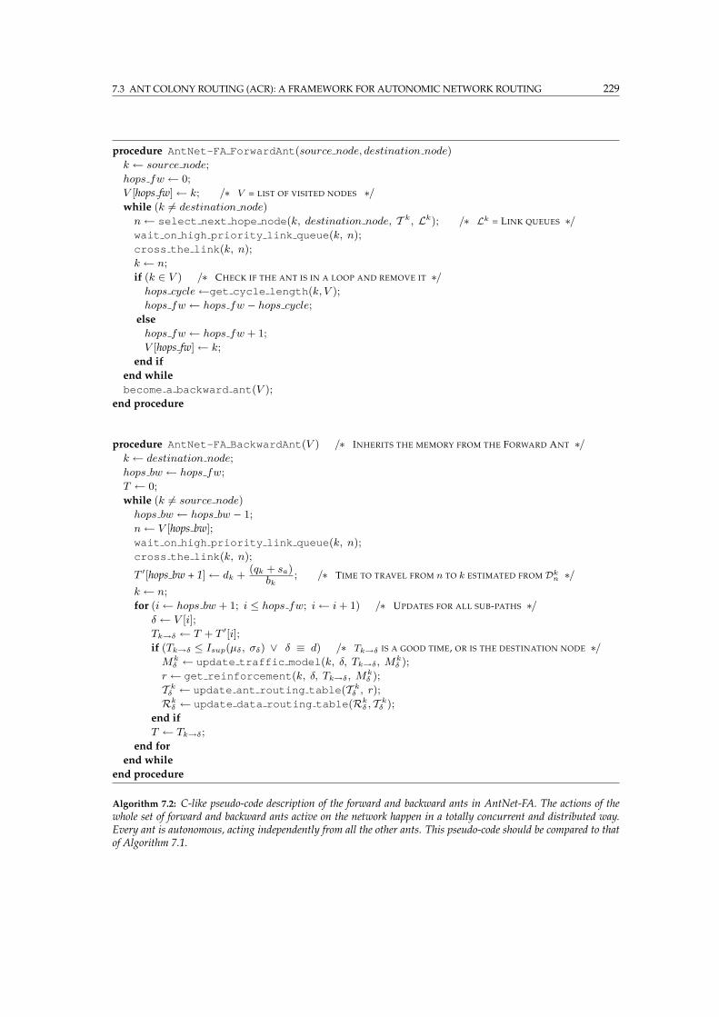
7.3 ANT COLONY ROUTING (ACR): A FRAMEWORK FOR AUTONOMIC NETWORK ROUTING 229
procedure AntNet-FA ForwardAnt(source node, destination node)
k ← source node;
hops fw ← 0;
V [hops fw]← k; /∗ V = LIST OF VISITED NODES ∗/
while (k 6= destination node)
n← select next hope node(k, destination node, T k, Lk); /∗ Lk = LINK QUEUES ∗/
wait on high priority link queue(k, n);
cross the link(k, n);
k ← n;
if (k ∈ V ) /∗ CHECK IF THE ANT IS IN A LOOP AND REMOVE IT ∗/
hops cycle←get cycle length(k, V );
hops fw ← hops fw − hops cycle;
else
hops fw ← hops fw + 1;
V [hops fw]← k;
end if
end while
become a backward ant(V );
end procedure
procedure AntNet-FA BackwardAnt(V ) /∗ INHERITS THE MEMORY FROM THE FORWARD ANT ∗/
k ← destination node;
hops bw ← hops fw;
T ← 0;
while (k 6= source node)
hops bw ← hops bw − 1;
n← V [hops bw];
wait on high priority link queue(k, n);
cross the link(k, n);
T ′[hops bw + 1]← dk +(qk + sa)
bk; /∗ TIME TO TRAVEL FROM n TO k ESTIMATED FROM Dk
n ∗/
k ← n;
for (i← hops bw + 1; i ≤ hops fw; i← i + 1) /∗ UPDATES FOR ALL SUB-PATHS ∗/
δ ← V [i];
Tk→δ ← T + T ′[i];
if (Tk→δ ≤ Isup(µδ, σδ) ∨ δ ≡ d) /∗ Tk→δ IS A GOOD TIME, OR IS THE DESTINATION NODE ∗/
Mkδ ← update traffic model(k, δ, Tk→δ, Mk
δ );
r ← get reinforcement(k, δ, Tk→δ, Mkδ );
T kδ ← update ant routing table(T k
δ , r);
Rkδ ← update data routing table(Rk
δ , T kδ );
end if
T ← Tk→δ;
end for
end while
end procedure
Algorithm 7.2: C-like pseudo-code description of the forward and backward ants in AntNet-FA. The actions of thewhole set of forward and backward ants active on the network happen in a totally concurrent and distributed way.Every ant is autonomous, acting independently from all the other ants. This pseudo-code should be compared to thatof Algorithm 7.1.
230 7. ACO ALGORITHMS FOR ADAPTIVE ROUTING
tables, such that these tables can be in turn used by the local stochastic control policy. The genera-
tion of the ant agents is expected to be adaptive and to follow both proactive and reactive strategies.
Moreover, the ant agents do not need anymore to have all the same characteristics. On the con-
trary, diversity at the level of both the value of their parameters and of their actions can play and
important role to cope with the intrinsic non-stationarity and stochasticity of network environ-
ments.
REMARK 7.15 (General characteristics of ACR): ACR defines the routing system as a distributed
society of both static and mobile agents. The static agents, called node managers, are connected to
the nodes and are involved in a continual process of adaptive learning of pheromone tables, that is,
of arrays of variables holding statistical estimates of the goodness of the different control actions locally
available. The control actions are expected to be issued on the basis of the application of stochastic
decision policies relying on the local pheromone values. The mobile, ant-like agents, play the role of
either active perceptions or effectors for the static agents, and are generated proactively and on-demand.
Node managers are expected to self-tune their internal parameters in order to adaptively regulate the
generation and the characteristics of these ancillary agents. In this way they are involved in two levels of
learning activities. The active perceptions carry out exploratory tasks across the network and gather
the collected non-local information back to the node managers. The effectors carry out ad hoc tasks, and
base their actions on pre-compiled deterministic plans (opposite to the active perceptions, that make use of
stochastic decisions and adapt to local conditions).
Using the language of the ant metaphor, passing from AntNet to ACR equals to moving from a colony
of ants to a society of multiple ant colonies, with each colony being an autonomic element devoted to
manage the activities of a single network node in social agreement with all the other colonies.
The ACR’s society of heterogeneous agents well matches forthcoming scenarios, in which net-
works will be likely populated by node agents and mobile agents. With these lasts carrying their
own code and specifications, moving across the networks, acting and interacting with other mo-
bile or node agents. They will be able to adapt themselves to new situations, possibly learn from
past experience, replicate if necessary or remove themselves if not useful anymore, cooperate
and/or compete with other agents, and so on.18 This picture will be likely closer and closer to
reality with the networks becoming more and more active (e.g., [420, 438]). That is, such that
packets will be able to carry their own execution or description code and all the network nodes
will be able to perform, as normal status of operations, customized computations on the packets
passing through them. Nowadays networks are more like a collection of high speed switching
boxes, but in the future those boxes will be replaced by “network computers” and the whole
network will likely appear as a huge multiprocessor system.
The organization envisaged by ACR is in accordance with the recent vision of autonomic
computing [250], that is, of computing systems that can manage themselves given high-level ob-
jectives from the administrators. ACR defines the generalities of a multi-agent society based on
the integration of the ACO’s philosophy with ideas from the domain of reinforcement learning,
with the aim of providing a meta-architecture of reference for the design and implementation of
fully autonomic routing systems. In fact, the node managers are expected to proactively monitor,
experiment with, and tune their own parameters in order to learn to issue effective decisions in
response to the different possible events and traffic scenarios. Each node manager is equipped
with a repertoire of basic strategies for control and monitoring actions. Adaptively and au-
tonomously the node manager optimizes the parameters of these strategies acting in accordance
18 Agent technology is receiving an ever increasing attention from telecommunication system engineers, researchersand practitioners. Agent modeling account in a straightforward way for the modularity of network components and,more importantly, they overcome the typical client-server model of communication since they can carry their own exe-cution code and they can be used as autonomous component of a global distributed and fault-tolerant system (among anumber of ever increasing works, see for example [220, 259, 206, 424, 265, 432]).
7.3 ANT COLONY ROUTING (ACR): A FRAMEWORK FOR AUTONOMIC NETWORK ROUTING 231
to social agreements with the other node managers. Each node manager is a fully autonomic el-
ement active in self-tuning and optimization by learning. On the other hand, the whole system
of node managers give raise to a fully autonomic routing system aimed at providing a traffic-
adaptive routing policy which is optimized at the network level.
7.3.1 The architecture
In the ACR framework the network is under the control of a system of distributed and adaptive
agents θk, one for each node k of the network. Each controller θk, also called a node manager, is
static (i.e., non-mobile) and its internal status is defined by the local values of pheromone tables
T θk (and also of heuristic arrays), as well as by other additional data structures ad hoc for the
problem at hand. Each entry in the pheromone array is associated to a different control action
locally available to the controller, and represents a statistical estimate of the goodness (e.g., util-
ity, profit, cost-to-go, etc.) of taking that action. The controller adopts a stochastic decision policy
which is parametrized by the pheromone and heuristic variables. The target of each controller
is to locally, and in some sense independently, learn a decision policy in terms of pheromone
variables such that the distributed society of controllers can jointly learn a decision policy opti-
mizing some global performance. Each controller is expected to learn good pheromone values by
observing the network environment, as well as the effect of its decisions on it, and making use of
these observations to adaptively change the pheromone values as well as other parameters regu-
lating its monitoring and control actions. Observations can be both local and non-local. Ant-like
agents are responsible for carrying out non-local observations and bringing back useful informa-
tion to the node managers. At each time the node manager must decide which kind of “action”
(local observation, remote perception, data routing, etc.) looks more appropriate according to
current status, requirements, and estimated costs/benefits.19 The local decision must be issued
taking into account the fact that the set of all node managers act concurrently and without any
form of global coordination. That is, the nodemanagers must act socially and possibly cooperate
in order to obtain positive synergy.
More specifically, the control architecture defined by the ACR framework is designed in the
terms of a hierarchical society composed of the following classes of agents:
Node managers: adaptive learning agents statically bounded to the nodes (one for each node).
They are all situated at the same hierarchical level. Each node manager autonomously
control the node activities (e.g., data routing and performance monitoring) on the ba-
sis of stochastic decision policies whose parameters, in the form of locally maintained
pheromone variables, are the main object of learning.
Active perceptions: mobile ant-like agents that are explicitly generated by the node managers
to collect non-local information (e.g., discovery of new routing paths). They have char-
acteristics of local adaptivity, might learn at individual level, and make use of stochastic
decision policies.
Effectors: mobile ant-like agents generated by the node managers to carry out pre-compiled
and highly specialized tasks (e.g., reserve and free network resources). They are expected
to adopt deterministic policies.
The dynamics of the whole network control system is driven by the node managers, while
both active perceptions and effector agents are generated in order to support node managers
activities. Generation dynamics can be based on both proactive and on-demand strategies in order
to deal effectively with the characteristics of the network at hand.
19 See for instance [219] for general discussions on decision systems that have to repeatedly decide between controland observation actions.
232 7. ACO ALGORITHMS FOR ADAPTIVE ROUTING
The terms “perceptions” and “effectors” suggest the interpretation of the node managers
as static robotic agents acting in the physically constrained network environment. On the other
hand, using the language of the ant metaphor, each node manager can be seen in the terms of a
single colony of ant-like agents. Learning processes happen as usual at the level of the colony
but are now concentrated on a node, while the ant agents, the active perceptions, are adaptively
generated in order to collect specific information or to reserve/free resources for the colony.
The ensemble of all the colonies constitutes a society of colonies, that must find the right level of
cooperation in order to obtain effective synergistic behaviors. Under this new point of view, a
greater emphasis is put on the activities at the nodes, which become the main actors of the whole
system, with learning happening at two levels, both at the level of the single nodes (the colonies)
and at the level of the ensemble of all the nodes (the colonies’ society). In the following we will
use interchangeably the terms nodemanager and colonymanager. Also the terms ant-like agent,
perception ant (effector ant), and active perception (effector agent), will be used interchangeably.
7.3.1.1 Node managers
The first task of a nodemanager consists in gathering data for building and continually updating
pheromone variables. Node managers can passively observe the local dynamics of traffic flows
and packet queues. However, this information might be in general insufficient to effectively
accomplish the node activities because of its intrinsic incompleteness. Therefore, node man-
agers need also to expand their “sensory field” with the adaptive generation of active perceptions
agents ξθk(t), that is, ant-like mobile agents that leave the node at time t, carry out some network
exploration activities, and gather back to the colony manager the information it requires after
some possibly short time delay. The term “active perception” is referred to both the facts that
a non-local perceptual act is explicitly issued and that each of these perceptual acts are actually
generated with a possibly different set of parameters in order to precisely get information about
a specific area of the network by using specific parameters concerning the path-following strat-
egy. That is, in general, ξθk(t1) 6= ξθk(t2), for t1 6= t2. This means that a node manager has a high
degree of control over the type of information that must be collected by its remote sensors, the
ant-like agents.
The design of node managers involves three main general aspects. That is, the definition of
the strategies for: (i) the scheduling of the active perceptions, (ii) the definition of the internal
characteristics for the generated perceptions, and (iii) the use of the gathered information in or-
der to learn effective decision policies and tune other internal parameters regulating for instance
the proactive scheduling of active perceptions. It is clear that a wide range of possible strategies
exists, depending on the specific characteristics of the problem at hand. Nevertheless, some gen-
eral strategies can be readily identified. Each of the three subsections that follow considers one
of the aspects (i-iii) and discusses in very general terms possible problems and solutions.
Scheduling of active perceptions
The set Θ = θ1, θ2, . . . , θN of all node managers virtually constitutes an agent society, in the
sense that node managers must behave socially since all of them equally contribute to the global
network performance. That is, generation of the perceptions must happen in order to safe-
guard the overall social welfare: each node must find the right tradeoff between gathering large
amounts of information and not creating congestion that in turn would either have a negative
impact on data routing or not allow the other node managers to gather the information that they
might need. It is apparent that the issue of the scheduling of the ant-like agents is central in ACR, as
it is in all ACO algorithms since they are all based on repeated agent generation for information
sampling.
7.3 ANT COLONY ROUTING (ACR): A FRAMEWORK FOR AUTONOMIC NETWORK ROUTING 233
REMARK 7.16 (Reactive and proactive information gathering): In ACR the ant-like mobile agents
can be generated by the node managers according to both reactive (on-demand) and proactive strategies.
In particular, the proactive strategies are not necessarily based on a fixed frequency scheme but on the
contrary are expected to be adaptive in order to find a good tradeoff between information gathering and
congestion induced by control packets.
Some general strategies for both the reactive and proactive generation of ant-like agents can
be identified. The list that follows is aimed at clarifying in which general situations ant-like
agents are “expected” to be generated and the general modalities of these generations. That
is, we point out some common problems/situations and we suggest some general solutions.
More concrete examples of mixing on-demand and proactive generation are provided by the
descriptions of AntNet+SELA and AntHocNet.
On-demand generation of active perceptions. Four classes of events can automatically trigger
the generation of new perception ants:
1. Setup of a new application: In the case of a best-effort connection-less network, at the
start-up of a new application As→d a burst of m ∝ |N (s)| new perception agents can
be generated toward d by θs to collect up-to-date information about the paths d. In
practice, active perceptions can be broadcast to the local set of neighbors, and then
move toward d using pheromone information.
In the case of connection-oriented and/or QoS networks, these setup ants play a more
critical role. In fact, they have to actually find (and possibly reserve) the path(s) to
allocate the application flow. A possible behavior of the perception agents in this
case is described more in detail in the following referring to the solution envisaged in
AntNet+SELA.
2. Major change in the traffic patterns: If the information associated to some newly ac-
quired data seems to strongly disagree with previously learned information, new
perceptions can be fruitfully generated in order to confirm or not the changes. For
instance, if the traveling time Ts→d reported by an ant agent indicates a value much
larger than the one estimated up to that moment going through the same next hop,
then it might be worth to get a clearer understanding of the traffic situation along the
path. In fact, the unexpected value could have been caused either by “wrong” choices
made by the perception agent due to a high level of stochasticity in its decision policy,
or by some new congestion along the path. If the involved next hop was among the
best ones so far for d, then before either keeping trusting it or reducing its goodness, it
can be worth to generate further perception agents with destination d through some
of the other outgoing links in order to gather more extensive information.
This behavior can be effectively seen in the terms of a local feedback loop between
monitoring of the network performance and issuing of control actions according to the
fact that the monitored performance is either poor or has significantly changed.
3. Request for or notification from a new destination node: According to the discussion in
Subsection 7.1.3.1 and in particular in the Remark 7.6 of the same subsection, it is
clear that in some cases a destination which is not yet present in the node routing
table might be requested (or, equivalently, a new node entering the network might
advertise its presence). In these cases perception agents need to be generated to
gather information about the new destination. This might be a rather common sit-
uation in mobile ad hoc networks. For instance, in AntHocNet, so-called reactive
setup ants search for a new destination by following pheromone information when
this is present at the current node, or being radio broadcast when no information is
available.
234 7. ACO ALGORITHMS FOR ADAPTIVE ROUTING
4. Topological failure: After the failure of a local link, or, equivalently, the disappearing
of a neighbor node, it might be necessary to generate perception agents in order to
gather fresh information about those destinations that were reached through that
link/node. This situation is quite common in networks with frequent topological
alterations, like the mobile ad hoc ones. However, since ACR instances make use of
multipath routing (because of the use of a stochastic decisions based on pheromone
values), several equally good alternatives are expected to be always available. Such
that it might be not strictly necessary to “recover” from the failure event since good
“backup” paths are likely made available. Again, in AntHocNet, ants are generated
only if the broken link was the choice of election to reach some of the used network
destinations, and/or no other equally good alternatives seem to be locally available.
When alternatives are available, some (effector) ant agents are however radio broad-
cast in order to notify neighbors about major changes in the routing table due to the
broken link.
Proactive generation of active perceptions. A background flow ωk of active perception agents
is continually and independently generated by each node manager θk to proactively keep
an updated view of the overall network status, and for the purpose of maintenance of the
paths used to route current traffic sessions. That is, proactive perceptions serve to be
ready for future traffic requests and to maintain and/or improve the quality of the cur-
rent ones. For what concerns routing in particular, proactive perceptions allow to main-
tain for each destination a bundle of paths with an associated measure of quality in the
form of pheromone value. Each path can be used either for multipath data spreading or as
alternate path in case of failures or sudden congestion.
The frequency of the proactive background flow is in general expected to be adaptive in
ACR instances, whereas it was heuristically assigned as a constant value in AntNet and
AntNet-FA. While the experimental results reported in Figure 8.17 in Subsection 8.3.6 sug-
gest that AntNet is quite robust with respect to the choice of the background frequency,
they also show that, with an appropriate tuning that depends on the overall network sce-
nario, performance can be appreciably improved. In general, answering the question “At
which rate control/routing agents should be generated ?” is at the same time extremely
difficult and of fundamental importance for any adaptive and social scheme. As pointed
out before, it is necessary to find a good tradeoff between frequency in information gath-
ering and generated congestion.
In principle, more control packets mean more precise and up-to-date information but also
control-induced congestion. However, control overhead should not be measured on an
absolute scale (as it is often done) but rather in relationship to the network performance
that it allows to obtain. A control algorithm that makes use of more control packets has
not to be seen in a negative way if those extra packets allow to obtain much better perfor-
mance, and at the same time performance scales well with network size and transmission
characteristics.20 The use of adaptive generation schemes precisely address this problem,
in principle allowing to optimize over the time the generation of control packets versus the
obtained performance.
Focusing on routing, a few major aspects have to be taken into account in the adaptive
definition of ωk: (i) the local transmission bandwidth, (ii) the minimal transmission band-
width across the network, (iii) the input traffic profile, (iv) the relative load generated by
20 For instance, the generation of 3-4 control agents per second (more or less the same frequency used in the AntNetexperiments) at each node of a backbone network with transmission links of more than 1 Gbits/sec cannot not be con-sidered as a significant overhead. On the other hand, the same overhead might be not negligible in the case of networkswith link bandwidths less than of 1 Mbits/sec or with shared wireless links.
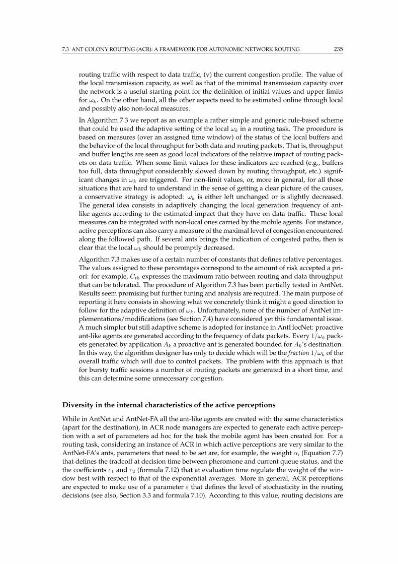
7.3 ANT COLONY ROUTING (ACR): A FRAMEWORK FOR AUTONOMIC NETWORK ROUTING 235
routing traffic with respect to data traffic, (v) the current congestion profile. The value of
the local transmission capacity, as well as that of the minimal transmission capacity over
the network is a useful starting point for the definition of initial values and upper limits
for ωk. On the other hand, all the other aspects need to be estimated online through local
and possibly also non-local measures.
In Algorithm 7.3 we report as an example a rather simple and generic rule-based scheme
that could be used the adaptive setting of the local ωk in a routing task. The procedure is
based on measures (over an assigned time window) of the status of the local buffers and
the behavior of the local throughput for both data and routing packets. That is, throughput
and buffer lengths are seen as good local indicators of the relative impact of routing pack-
ets on data traffic. When some limit values for these indicators are reached (e.g., buffers
too full, data throughput considerably slowed down by routing throughput, etc.) signif-
icant changes in ωk are triggered. For non-limit values, or, more in general, for all those
situations that are hard to understand in the sense of getting a clear picture of the causes,
a conservative strategy is adopted: ωk is either left unchanged or is slightly decreased.
The general idea consists in adaptively changing the local generation frequency of ant-
like agents according to the estimated impact that they have on data traffic. These local
measures can be integrated with non-local ones carried by the mobile agents. For instance,
active perceptions can also carry ameasure of themaximal level of congestion encountered
along the followed path. If several ants brings the indication of congested paths, then is
clear that the local ωk should be promptly decreased.
Algorithm 7.3 makes use of a certain number of constants that defines relative percentages.
The values assigned to these percentages correspond to the amount of risk accepted a pri-
ori: for example, Cth expresses the maximum ratio between routing and data throughput
that can be tolerated. The procedure of Algorithm 7.3 has been partially tested in AntNet.
Results seem promising but further tuning and analysis are required. The main purpose of
reporting it here consists in showing what we concretely think it might a good direction to
follow for the adaptive definition of ωk. Unfortunately, none of the number of AntNet im-
plementations/modifications (see Section 7.4) have considered yet this fundamental issue.
A much simpler but still adaptive scheme is adopted for instance in AntHocNet: proactive
ant-like agents are generated according to the frequency of data packets. Every 1/ωk pack-
ets generated by application Ak a proactive ant is generated bounded for Ak’s destination.
In this way, the algorithm designer has only to decide which will be the fraction 1/ωk of the
overall traffic which will due to control packets. The problem with this approach is that
for bursty traffic sessions a number of routing packets are generated in a short time, and
this can determine some unnecessary congestion.
Diversity in the internal characteristics of the active perceptions
While in AntNet and AntNet-FA all the ant-like agents are created with the same characteristics
(apart for the destination), in ACR node managers are expected to generate each active percep-
tion with a set of parameters ad hoc for the task the mobile agent has been created for. For a
routing task, considering an instance of ACR in which active perceptions are very similar to the
AntNet-FA’s ants, parameters that need to be set are, for example, the weight α, (Equation 7.7)
that defines the tradeoff at decision time between pheromone and current queue status, and the
the coefficients c1 and c2 (formula 7.12) that at evaluation time regulate the weight of the win-
dow best with respect to that of the exponential averages. More in general, ACR perceptions
are expected to make use of a parameter ε that defines the level of stochasticity in the routing
decisions (see also, Section 3.3 and formula 7.10). According to this value, routing decisions are
236 7. ACO ALGORITHMS FOR ADAPTIVE ROUTING
procedure ACR LocalFrequencyOfProactiveAgentGeneration(ω)if (routing throughput ≥ Cth · data throughput) LOCAL ROUTING THROUGHPUT SEEMS TOO HIGH. . .
if (waiting data bits ≥ C−
buf · total size of local buffers) . . . AND TOO MANY DATA PACKETS. . .
∆←C−
buf · total size of local buffers
waiting data bits; . . . DECREASE THE FREQUENCY
else if (waiting routing bits > Cw · waiting data bits) . . . TOO MANY ROUTING PACKETS . . .
∆←Cw · waiting data bits
waiting routing bits; . . . DECREASE THE FREQUENCY
else if`
(waiting data bits < C+
buf · total size of local buffer) ∧(waiting data bits > C+
w · waiting routing bits) ∨(waiting routing bits < C+
wr · total size of local buffers)´
. . . QUEUES ALMOST EMPTY. . .
∆← 1 +waiting data bits
C+
buf · total size of local buffer; . . . INCREASE THE FREQUENCY
else . . . THE SITUATION IS HARD TO EVALUATE. . .∆← 1; . . . CONSERVATIVE STRATEGY: DO NOT CHANGE
end if
else if ((waiting data bits ≥ C−
buf · total size of local buffers) ∧(waiting routing bits > C−
w · waiting data bits)) . . . ROUTING QUEUES OK BUT BUFFERS ARE FULL. . .
∆←C−
w · waiting data bits
waiting routing bits; . . . DECREASE FREQUENCY
else . . . BOTH THROUGHPUT AND BUFFERS ARE OK. . .∆← 1 + ǫ; . . . INCREASE FREQUENCY
end ifω ← ω ·∆;
end procedure
Algorithm 7.3: Pseudo-code for the example of adaptive setting of the frequency for the proactive generation of activeperceptions by a node manager. Cth, C−
buf , C+
buf , C−
w , C+w , C+
wr, ǫ are assigned constants. For instance, a reasonable
assignment of values might be as follows: Cth = 0.2, C−
buf = 0.1, C+
buf = 0.001, C−
w = 0.2, C+w = 1.2, C+
wr =0.0001, ǫ = 0.001.
taken following a random proportional scheme or strategies more greedy toward the best next
hop(s). For instance, at the setup time of a new application in a QoS network, on-demand per-
ceptions searching for a QoS-feasible path are expected to behave more greedily than proactive
perceptions exploring the network (see also the description of AntNet+SELA).
The probabilistic selection of (some of) the agent characteristics determines in the agent pop-
ulation a high level of diversity, which is in general seen as an effective feature in a multi-agent
system operating in non-stationary environments, since it is expected to provide robustness, and
favor global adaptability and task distribution.21 The assignment of parameter values accord-
ing to some sampling procedure avoids the assignment of critical crisp values to the algorithm
parameters. On the contrary, it might be necessary to define only the parametric characteristics
of statistical distributions (e.g., Gaussian) from which the parameter values are sampled from
during the algorithm execution. In principle, also the characteristics of centrality and disper-
sion of the sampling distributions can be in turn adapted online according to the monitored
performance.
21 At least this is what is commonly observed in Nature’s systems (e.g., see [168, 3]). Some general studies on artificialmulti-agent systems [10, 239, 240] further support this view.
7.3 ANT COLONY ROUTING (ACR): A FRAMEWORK FOR AUTONOMIC NETWORK ROUTING 237
Learning strategies
Node managers can make use of any appropriate strategy to learn effective decision policies
concerning data routing, monitoring, agent generation, parameters setting, etc. The pheromone
variables are the main object of learning, since they play the role of parameters of the stochastic
decision policies. Generally speaking, stochastic decision policies appears as more appropriate
than deterministic ones to deal with the intrinsic characteristics of non-stationarity and distribu-
tion (i.e., hidden global state) of network environments. Moreover, in the case of routing tasks,
the adoption for data routing of a stochastic policy based on pheromone values likely results
in spreading data over multiple paths and automatically providing load balancing, that we see as
positive features.
In the case of AntNet and AntNet-FA the adopted learning strategies are quite essential. An
example of amore complex example learning architecture and strategy is given inAntNet+SELA,
in which the node managers are stochastic estimator learning automata (SELA) [430, 330] and make
use of link-state tables to provide guaranteed QoS routing in ATM networks. Stochastic learning
automata, have been used in early times [331, 334] to provide fully distributed adaptive routing.
Their main characteristics consists in the fact that they learn by induction: no data are exchanged
among the controllers. They only monitor local traffic and try to get an understanding of the
effectiveness of their routing choices. In AntNet+SELA the static inductive learning component
is enhanced by using the ants as active perceptions in order to gather also non-local information
to keep up-to-date the link-state routing table in the perspective of rapidly allocating resources
for multipath QoS routing when necessary.
7.3.1.2 Active perceptions and effectors
Active perceptions are mobile agents explicitly generated by node managers for the purpose of
non-local exploration and monitoring. Most of the general characteristics that can be attributed
to active perception agents have been already described in the previous subsections. Here we
complete the general picture pointing out some additional aspects.
• The model of interaction between perceptions and node managers envisaged by ACR is
that typical of agent and object-oriented programming. Node managers and active percep-
tions are situated at a different hierarchical level. The active perception is subordinate to
the node manager, that creates it for the purpose of collecting useful non-local informa-
tion. Therefore, the hierarchically lower active perception should not directly modify the
internal state of a node manager. That is, perceptions are not expected to directly modify
the node manager’s data structures (e.g., the pheromone table). Perceptions can only com-
municate to node managers the information they have collected along the path, while is
the node manager’s responsibility and decision to use or not this information to update its
private data structures. There are at least three reasons to follow this behavior. First, by
design the component for “intelligent” processing of sensory data is supposed to be the
node manager and not its perception. Second, for security reasons: what if a competing and
“malicious” network provider generates intruder perceptions carrying wrong information
and evil objectives? ACR does not directly address this class of problems, but shielding a
potential enemy from gaining access to the main node data structures is clearly an issue
of critical importance. Third, a direct modification of the node data structures would be
against the principles of information hiding at the basis of all the modern (object-oriented)
programming. The perception does not need to know about which kind of models, struc-
tures, data are used by the node managers. All it does need to know is the protocol to
communicate its data to the node manager. In this way, data representations and learning
algorithms internal to the nodes can either change very often or even being different from
238 7. ACO ALGORITHMS FOR ADAPTIVE ROUTING
node to node. The only important thing from the point of view of the perceptions is that
the local communication interface does not change.
• Active perceptions can have the peculiar characteristic of replicating (or, proliferating) when
there is more than one single good alternative. For instance, let Fs→d be a “forward” per-
ception moving from s to d. At the current node k, an AntNet ant would just pick-up one
single link proportionally to its probability and move through it. Acting in this way, the
ant discards other potentially promising links. On the other hand, if after the calculations
of formula 7.7 there is no one single best link but a set n1, n2, . . . , nb, b > 1, of more or less
equally good links, then the perception might replicate in b copies. Each copy can proceed
on a different link ni, i = 1, . . . , b to explore all these equivalent alternatives. Clearly, to
avoid an uncontrolled proliferation of perception agents, some limits must be heuristically
assigned on the allowed number of replicas.
For instance, in AntHocNet, when no pheromone information for the ant destination is
present at the current node, the ant is broadcast. This equals to considering all the links
as equally good, such that the ant is transmitted to each possible neighbor. Clearly, if
multiple broadcastings happen, the network can easily get flooded (and congested) by
routing packets. Therefore, some heuristics are applied in order to kill the forward ant
(e.g., ants that have proliferated from the same original ant and that arrive at a same node
with no pheromone are destroyed if they have been already broadcast a certain number of
times, or if their traveling time and number of hops do not score favorably with those of
previous passed by ants).
• Active perceptions can be of different type, according to the different task they will be in-
volved in. Clearly, different tasks usually require also different characteristic (e.g., level of
stochasticity). While in AntNet and AntNet-FA all the ants are involved in the same task
such that they all have the same type and characteristics, in both AntNet+SELA and An-
tHocNet there are several types of active perceptions, and the different types have different
internal characteristics.
• There is not somuchmore to say about the effector agents. We have already introduced them
when talking about AntHocNet’s ants that notify pheromone updates after a link failure.
Also in AntNet+SELA effector agents are used: to take care of allocation and deallocation
of QoS resources. In general effectors are “blind” executor agents, used to carry out tasks
whose specifications have been completely defined at the level of the generating node
manager.
7.3.2 Two additional examples of Ant Colony Routing algorithms
Both AntNet and AntNet-FA can be seen as instances of the more general ideas of the ACR
framework. On the other hand, in both AntNet and AntNet-FA all the ants are generated ac-
cording to the same fixed proactive scheme, have the same characteristics and behavior, and
the notion of node manager has not been made explicit, such that there is little “intelligence” at
the nodes. In a sense, AntNet and AntNet-FA results in a rather natural way from the general
ACO’s guidelines and from the adaptation of the main ideas of previous ACO implementa-
tions for static combinatorial problems. Even though these characteristics might be a quite good
match for the considered cases of wired best-effort networks, it is apparent that smarter node
managers, as well as increased levels of heterogeneity and adaptivity, might be useful if not
necessary components to deal effectively with network scenarios that are either highly dynamic
(e.g., mobile ad hoc networks) or include some forms of QoS provisioning. Therefore, in order to
show how the ACR’s ideas find their natural application in such complex and highly dynamic
7.3 ANT COLONY ROUTING (ACR): A FRAMEWORK FOR AUTONOMIC NETWORK ROUTING 239
scenarios (or, equivalently, how the basic AntNet and AntNet-FA design can be extended and
adapted to deal with the increased complexity), we briefly describe in the two next subsections
two additional routing algorithms: AntNet+SELA [126] and AntHocNet [128, 155, 129].
AntNet+SELA is a intended for guaranteed QoS routing in ATMnetworks, while AntHocNet
is for routing in mobile ad hoc networks. AntNet+SELA and AntHocNet will be not described
in all their details. In fact, in order to properly discuss all the components of these algorithms, an
in-depth introduction to both QoS and mobile ad hoc networks issues is required. However, this
would likely require an additional chapter, that would make this thesis unnecessarily too long.
Moreover, AntNet+SELA has never been fully tested, such that it is more a model than a real
implementation, while AntHocNet is still under intensive development, and only preliminary,
even if extremely encouraging, results are at the moment available (they will be shortly reported
in the next chapter).22
7.3.2.1 AntNet+SELA: QoS routing in ATM networks
The transmission capacity of current network technology allows to support multiple classes of
network services associated to different QoS requirements. QoS routing is the first, essential step
toward achieving QoS guarantees. It serve to identify one or more paths that meet the QoS re-
quirements of current traffic sessions while possibly providing at the same time efficient utiliza-
tion of the network resources in order to satisfy the QoS requests of also future traffic sessions.
When a new user application arrives and requires some specific network resources, the local
connection admission control (CAC) component makes use of the available routing information
to evaluate at which degree the QoS requirements can be satisfied and to decide if the session
can be accepted or not. Several different general models (e.g., IntServ, DiffServ, MPLS, ATM)
have been proposed so far to deal with the several issues involved in this general picture: reser-
vation vs. non-reservation of the resources, classes of type of provided services, deterministic
vs. statistical guarantees, mechanisms for evaluation (and allocation) of the available resources,
levels of negotiation between the user and the CAC component, rerouting vs. non-rerouting of
the applications, use of multiple paths vs. single path, etc. (there is an extensive literature on
QoS, good and quite comprehensive discussions can be found for example in [398, 285, 440]).
AntNet+SELA [126] focuses on the case of providing QoS in ATM networks for generic vari-
able bit rate (VBR) traffic. For this class of networks virtual circuits can be established either per
flow or per destination basis such that physical reservation of resources is possible. Therefore,
statistically guaranteed quality of service can be provided.
In AntNet+SELA the node managers, that are directly responsible for both routing and ad-
mission decisions, are designed after the stochastic estimator learning automata (SELA) [430] used
in the SELA-routing distributed system [8]. They make use of active perceptions to collect non-
local information according to both on-demand and proactive generation schemes. The active
perceptions are designed after the AntNet-FA ants. Also effectors agents are used, to tear down
paths and to gather specific information about traffic profiles of running applications.
Node managers in SELA-routing
In order to understand the overall behavior of the algorithm, is first necessary to briefly ex-
plain the characteristics of the SELA-routing system, in which each node manager is a stochastic
learning automaton. In general terms, a stochastic learning automaton is an finite-state machine
that interacts with a stochastic environment trying to learn the optimal action the environment
22 More conclusive and comprehensive experiments about AntHocNet are expected to result fromDucatelle’s doctoralwork, as explained in Footnote 4.
240 7. ACO ALGORITHMS FOR ADAPTIVE ROUTING
offers. The automaton chooses an action according to an output function and a vector of prob-
abilities scoring the goodness of every possible action. After executing the action, it receives a
reward/feedback signal from the environment and uses the signal to update a statistical model
(e.g., a moving average of the received rewards and of the last time an action has been selected)
of the expected feedback associated to every possible action. The actions are then sorted accord-
ing to the new estimates and the vector of probabilities is updated increasing the probability of
the action with the new best estimated reward and lowering the probabilities for all the other ac-
tions. In the specific case of SELA-routing, the node managers make use of a link-state database
and offline find the k-minimum-hop paths P1, . . . ,Pk for each destination. These k paths are the
set of actions available to the automaton. The behavior of the algorithm is then as follows:
Arrival of a new application: Whenever a new application asks for a QoS connection, the applica-
tion must communicate to the local node manager: (i) its traffic profile in terms of peak cell
rate, mean idle and burst periods, (ii) its QoS requests in terms of bandwidth, delay, delay
jitter, and loss rate.
Estimate of link utilization: The application’s characteristics are input to a fluid-flow approxima-
tion model to estimate the expected utilization ui for each link i on the k possible paths.
Environment feedback: For each possible action (path with n hops) the feedback from the envi-
ronment is computed as: aj = M −∑ni=1,ui∈Pj
ui, whereM is a constant representing the
maximum number of hops that can be admitted in a path, ui ∈ [0, 1] and ui = 1 if ui is
greater than a threshold utrunk defined according to some trunk-reservation strategy.
Path selection: Order the actions according to the estimated feedback and select the action ajwith the best estimated feedback: aj > ai, ∀i, i 6= j (ties are resolved at random). If aj is a
minimum-hop path andmeets the QoS requirements then the path is accepted. Otherwise,
if aj is not a minimum-hop path but meets the QoS requirements and∑ni=1,ui∈Pj
ui <
utrunk, then the path is accepted. If none of these two sets of conditions are met, the next
path in the a’s sequence is considered until an acceptable path is found and the application
can start. If none of the paths meets the requirements, the application is rejected.
AntNet+SELA: description of the algorithm
In AntNet+SELA the node managers make use of ant-like agents in order to proactively up-
date their link-state database, take routing decision using fresh information about the candi-
date paths, and split and reroute the applications if useful/necessary. In particular, node man-
agers make use of two sets of active perceptions. The perceptions in one set behave exactly
like AntNet-FA ants, and are aimed at proactively building and maintaining pheromone ta-
bles for the perceptions (ants) in the second set, which are reactively generated at the setup of
a new application. These perceptions make use of the pheromone tables either to probe the
paths suggested for routing by the node manager or to discover other and possibly better paths.
Node managers make also use of effector agents, to gather information about the congestion
status over the allocated paths in order to update the parameters of fluid-flow model used
by node managers and/or to possibly reroute them. More in specific, the overall behavior of
AntNet+SELA is as follows:
• Perception agents (hereafter called proactive ants) are generated from every node manager
according to a proactive scheme. They behave like AntNet-FA ants, searching for paths
and updating the pheromone tables that are going to be used for routing also by other per-
ceptions. That is, the routing information used by the perception agents is different from
that used to route data, which is contained in the link-state tables of the node managers.
In this way, network exploration and routing of data traffic follow different dynamics.
7.3 ANT COLONY ROUTING (ACR): A FRAMEWORK FOR AUTONOMIC NETWORK ROUTING 241
• At the arrival of a new application, the node manager launches two groups of perceptions:
– Perceptions in the first group (path-probing setup ants) probe online the the k paths
suggested by the node manager path selection phase.
– Perceptions in the other group (path-discovering setup ants) make use of the pheromone
tables built by proactive ants to discover new QoS-feasible paths for the application.
• Ants in both groups temporary reserve resources for the applicationwhile theymove along
the paths.
• Path-discovering setup ants are created with different internal parameters, such that they
can be more or less greedy with respect to the current status of the link queues (parameter
α in Equation 7.7). Moreover, they always choose the link with the highest probability
(computed on the basis of ant-routing table).
• In the case that there is only a little difference between the best and the second best link, the
setup ant forks and both links are followed (however, to avoid uncontrolled multiplication
of ants, an ant is allowed the fork only once).
• If a followed path does not meet anymore the QoS requests, an effector ant is generated to
retrace back the setup ant path and free the allocated resources.
• Every setup ant which is able to arrive at destination following a QoS-feasible path comes
back and reports the information to the node manager. This information is also used to
revise the selection probabilities for the k paths.
• After the first setup ant is back (earlier than a maximum timeout delay), the application
can start sending packets.
• If more setup ants come back, the node manager decides about the opportunity to split or
not the application over multiple paths (e.g., if path superposition is very low it might be
quite effective to use multiple paths).
• Once the application is active, periodically some effectors agents (monitor ants) are proac-
tively sent over the allocated path(s) to collect information about the application traffic
profile and about the links’ usage. This information is used to update online the param-
eters of the fluid-flow approximation model used by the node managers to calculate the
environment feedback associated to the possible paths.
• The information reported by the monitor agents is also used to monitor the traffic over
established paths for the purpose of maintenance. If the network load becomes heavily
unbalanced and/or new resources are made available, the application can be gracefully
rerouted (or split).
• When the application ends its activities, effector agents are sent over the paths used by the
application in order to free the allocated resources.
• The system can be used to manage at the same time QoS traffic and best-effort traffic (via
the routing tables built by the proactive monitor ants).
AntNet+SELA contains several additional components with respect to both AntNet and
AntNet-FA: learning agents as node managers, reactive and effector agents, diversity in the
agent population, allocation and maintenance of virtual circuits, etc. However, all the three
algorithms are clearly designed according to the same philosophy, which is that that we have
tried to capture in the informal definition of ACR.
242 7. ACO ALGORITHMS FOR ADAPTIVE ROUTING
AntNet+SELA is a good example of how several aspect can andmust coexist in the same ant-
based routing system in order to cope effectively with the overall complexity of routing tasks.
Moreover, it is apparent the modularity of the approach: a different learning architecture can be
used for the nodemanagers in place of learning automata without requiringmajor modifications
in the structure and behaviors of the ant-like agents (whose task remains that of exploring and
gathering information).
No pseudo-code description is given for AntNet+SELA (as well as for AntHocNet). In
fact, these algorithms, are designed to deal with a number of different events (e.g., genera-
tion, forwarding, and processing of monitor, path-probing and proactive ant perceptions, as
well as of various effector agents), such that, for instance, the pseudo-code description of an
AntNet+SELA’s node manager would result in a finite state machine with several states and
state transitions. The pseudo-code of AntHocNet would result even more complex since An-
tHocNet has been implemented using a realistic packet-level simulator, such that the protocol
has to deal in practice with all the possible events that characterize a fully realistic protocol.
These facts would probably make the pseudo-code quite hard to follow and so quite useless for
the purpose of helping to get a clearer idea of the algorithm behavior.
7.3.2.2 AntHocNet: routing in mobile ad hoc networks
In recent years there has been an increasing interest in Mobile Ad Hoc Networks (MANETs). In
this kind of networks, all nodes are mobile and can enter and leave the network at any time.
They communicate with each other via wireless connections. All nodes are equal and there is
neither centralized control nor fixed infrastructure to rely on (e.g., ground antennas). There are
no designated routers: all nodes can serve as routers for each other, and data packets are for-
warded from node to node in a multi-hop fashion. Providing reliable data transport in MANETs
is quite difficult, and a lot of research is being devoted to this. Especially the routing problem is
very hard to solve, mainly due to the constantly changing topology, the lack of central control
or overview, and the low bandwidth of the shared wireless channel. In recent years a number of
routing algorithms have been proposed (e.g., see [371, 61, 399]), but even current state-of-the-art
protocols are quite unreliable in terms of data delivery and delay.
The main challenge of MANETs for ant-based routing schemes consists in finding the right
balance between the rates of agent generation and the associated overhead. In fact, from one
side, repeated path sampling is at the very core of ACR algorithms: more agents means that an
increased and more up-to-date amount of routing information is gathered, possibly resulting in
better routing. On the other side, an uncontrolled generation of routing packets can negatively
affect whole sets of nodes at once due to the fact that the radio channel is a shared resource
among all the nodes, such that multiple radio collisions can happen at the MAC layer with con-
sequent degradation of performance (this is especially true if the channel has low bandwidth).
In a MANET nodes can enter and leave the network at any time, as well as nodes can become
unreachable becomes of mobility and limitations in the radio range. Therefore, in general it is
not reasonable to keep at the nodes either a complete topological description of the network or
a set of distances/costs to all the other nodes (even at the same hierarchical level) as it can be
done, for instance, in the most of the cases of wired networks. These situations call for building
and maintaining routing tables on the basis of reactive strategies possibly supported by proactive
actions in order to continually refresh the routing information that might quickly become out-of-
date because of the intrinsic dynamism of the network.
This is the strategy followed in AntHocNet [128, 130, 155, 129], which is a reactive-proactive
multipath algorithm for routing in MANETs. The structure of AntHocNet is quite similar to
that of AntNet-FA with the addition of some components specific to MANETs that results in
the presence of several types of ant-like agents. In particular, the design of AntHocNet features:

7.3 ANT COLONY ROUTING (ACR): A FRAMEWORK FOR AUTONOMIC NETWORK ROUTING 243
reactive agents to setup paths toward a previously unknown destination, per-session proactive
gathering of information, agents for the explicit management of link failure situations (because
of mobility and limited radio range the established radio link between two nodes can easily
break). Node managers are not really learning agents as it was the case for AntNet+SELA, but
rather finite statemachines respondingmore or less reactively to external events. This is partially
due to the fact that in such highly dynamic environments it might be of questionable utility to
rely on approaches strongly based on detecting and learning environment’s regularities. In the
general case, some level of learning and proactivness is expected to be of some usefulness, but
at the same time the core strategy should be a reactive one. This has been our design philosophy
in this case.
The algorithm’s behavior is explained in the following subsections. Each subsection dis-
cusses the algorithm actions in relationship to a different subtask: (i) setup of routing informa-
tion, (ii) maintenance of established routes and exploration of new ones, (iii) data routing, (iv)
management of link failures.
Path setup
When a new data session to a destination d is started, the node manager at source node s reac-
tively sends out a setup ant for the purpose of searching for routes between s and d (unless, of
course the source already has routing information about the destination). Setup ants, as all the
other agents, always make use of higher priority queues with respect to data packets. Each node
which receives the setup ant either radio broadcast or unicast it according to the fact that it has or
not routing information about d in the routing table. The node to unicast the ants to is selected
according to the pheromone information. Broadcasting determines a sort of proliferation of the
original ant since each neighbor will receive a copy of it. This proliferation, if uncontrolled, can
be easily lead to an unwanted congestion. Therefore, setup ants are filtered according to the qual-
ity of the path followed so far in order to limit the generated overhead. When a node receives
several ants of the same generation (i.e., deriving from the same forward ant generated in s),
it will compare the path traveled by the ant to that of the previously received ants of the same
generation: only if its number of hops and travel time are both within a certain factor of that of
the best ant of the generation, it will forward the ant. Ants can get also killed on the way if their
number of hops exceeds a predefined time-to-live value, which is set according to the network
size.
Upon arrival at the destination d, the forward ant is converted into a backward ant which
travels back to the source, retracing the forward path. At each node i, it sets up a path towards
the original destination d creating or updating routing table entries T ind for the neighbor n it is
coming from. The entry will contain a pheromone value which represents an average of the
inverse of the cost, in terms of both estimated time and number of hops, to travel to d through n
from i.
Data routing
The path setup phase creates a number of paths between source and destination, indicated in
the datagram routing tables of the nodes. Data can then be forwarded between nodes accord-
ing to a stochastic policy parametrized by the data-routing tables, which are obtained from the
pheromone tables after a power-law transformation equivalent to that used in AntNet-FA.
The probabilistic routing strategy leads to data load spreading with consequent automatic
load balancing. This might be quite important in MANETs, because the bandwidth of the wire-
less channel is very limited. Of course, in order to spread data properly, adapting to the repeated
modifications in both the traffic and mobility patterns, it is customary to keep monitoring the
244 7. ACO ALGORITHMS FOR ADAPTIVE ROUTING
quality (and the existence) of the different paths. To this end the node managers generate proac-
tive maintenance ants (perceptions) and pheromone diffusion ants (effectors).
Path maintenance and exploration
While a data session is running, the nodemanager sends out proactive maintenance ants according
to the data sending rate (one ant every n data packets). They follow the pheromone values
similarly to data but have a small probability at each node of being broadcast. In this way
they serve two purposes. If an ant reaches the destination without a single broadcast it simply
samples an existing path. It gathers up-to-date quality estimates of this path, and updates the
pheromone values along the path from source to destination. If on the other hand the ant got
broadcast at any point, it will leave the currently known “pheromone-constrained” paths, and
explore new paths. However, we limit the total number of broadcasts of a proactive ant to a small
number (e.g., two) in order to avoid excessive agent proliferation. The effect of this mechanism
is that the search for new paths is concentrated around the current paths, so that we are looking
for path improvements and variations.
In order to guide the search more efficiently, node managers make use also of effector agents
termed pheromone diffusion ants: short messages resembling hello messages broadcast every t
seconds (e.g., t = 1 sec). If a node receives a pheromone diffusion agent from a new node n,
it will add n as a new destination in its routing table. After that it expects to receive an agent
from n every t seconds. After missing a certain number of expected messages (2 in our case),
n will be removed. Using these messages, nodes know about their immediate neighbors and
have pheromone information about them in their routing table. Pheromone diffusion ants also
serve another purpose: they allow to detect broken links. This allow nodes to clean up stale
pheromone entries from their routing tables. In the following we plan to make these agents
carrying more information (e.g., the list of neighbors).
Link failures
Node managers can detect link failures (e.g., a neighbor has moved far away) when unicast
transmissions (of data packets or ants) fail, or when expected pheromone diffusion agents were
not received. When a link fails, a node might loose a route to one or more destinations.
If the node has other next hop alternatives to the same destination, or if the lost destination
was not used regularly by data, this loss is not so important, and the node manager will just
update its routing table and broadcast an effector agent, termed failure notification ant. The agent
carries a list of the destinations it lost a path to, and the new best estimated end-to-end delay
and number of hops to this destination (if the node still has entries for the destination). All its
neighbors receive the notification and update their pheromone table using the new estimates. If
they in turn lost their best or their only path to a destination due to the failure, they will in turn
generate and broadcast a failure ant, until all nodes along the different paths are notified of the
new situation.
If the lost destination was regularly used for data traffic, and it was the node’s only alterna-
tive for this destination, the loss is important and the node should try to locally repair the path.
This is the strategy followed in AntHocNet, with the restriction that a node only repairs the path
if the link loss was discovered with a failed data packet transmission. After the link failure, the
node manager broadcasts a route repair ant that travels to the involved destination very alike
a setup ant: it follows available routing information when it can, and is broadcast otherwise
(with a limit of the maximum number of broadcasts). The node manager waits for a certain time
and if no backward route repair ant is received, it concludes that it was not possible to find an
alternative path to the destination which is then removed from the routing table, and a failure
notification ant is generated to advertise the new situation.
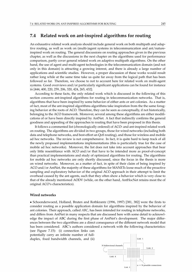
7.4 RELATED WORK ON ANT-INSPIRED ALGORITHMS FOR ROUTING 245
7.4 Related work on ant-inspired algorithms for routing
An exhaustive related work analysis should include general work on both multipath and adap-
tive routing, as well as work on (multi-)agent systems in telecommunication and ant/nature-
inspired work on routing. The general discussions on routing approaches given in the previous
chapter, as well as the discussions in the next chapter on the algorithms used for performance
comparison, partly cover general related work on adaptive multipath algorithms. On the other
hand, the use of agent and multi-agent technologies in the telecommunication domain (and not
only in this domain) is attracting a growing interest, and there is already a large number of
applications and scientific studies. However, a proper discussion of these works would result
rather long while at the same time take us quite far away from the logical path that has been
followed so far. Therefore, we choose to not to account here for related work on multi-agent
systems. Good overviews and/or particularly significant applications can be found for instance
in [444, 400, 220, 259, 206, 320, 424, 265, 432].
According to these facts, the only related work which is discussed in the following of this
section concerns ant-inspired algorithms for routing in telecommunication networks. That is,
algorithms that have been inspired by some behavior of either ants or ant colonies. As a matter
of fact, most of the ant-inspired algorithms algorithms take inspiration from the the same forag-
ing behavior at the roots of ACO. Therefore, they can be seen as conceptually, if not historically,
belonging to the ACO framework. Moreover, several among these algorithms are either modifi-
cations of or have been directly inspired by AntNet. A fact that indirectly confirms the general
goodness and appealing of the approaches to routing that have been proposed in this thesis.
It follows a commented list (chronologically ordered) of ACO- and ant-inspired related work
on routing. The algorithms are divided in two groups, those for wired networks (including both
data and telephone networks, and best-effort an QoS routing), and those for wireless andmobile
ad hoc networks. The review is not comprehensive. In fact, it is quite hard to keep track of all
the newly proposed implementations implementations (this is particularly true for the case of
mobile ad hoc networks). Moreover, the list does not take into account approaches that bear
only little resemblance with ACO and/or that have to be intended more as proof-of-concept
than practical implementations and study of optimized algorithms for routing. The algorithms
for mobile ad hoc networks are only shortly discussed, since the focus in the thesis is more
on wired networks. Moreover, as a matter of fact, in spite of their claim of being inspired by
ACO and/or AntNet, the majority of these algorithms for MANETs loose much of the proactive
sampling and exploratory behavior of the original ACO approach in their attempt to limit the
overhead caused by the ant agents, such that they often show a behavior which is very close to
that of the already mentioned AODV (while, on the other hand, AntHocNet retains most the of
original ACO’s characteristics).
Wired networks
• Schoonderwoerd, Holland, Bruten and Rothkrantz (1996, 1997) [381, 382] were the firsts to
consider routing as a possible application domain for algorithms inspired by the behavior of
ant colonies. Their approach, called ABC, has been intended for routing in telephone networks,
and differs from AntNet in many respects that are discussed here with some detail to acknowl-
edge the impact of ABC during the first phase of AntNet’s development. The major differ-
ences between the two algorithms are a direct consequence of the different network model that
has been considered. ABC’s authors considered a network with the following characteristics:
Link 4
N bidirectional channels
Link 1
Link 3n << N possible connections
Link 2
(see Figure 7.15): (i) connection links can
potentially carry an infinite number of full-
duplex, fixed bandwidth channels, and (ii)
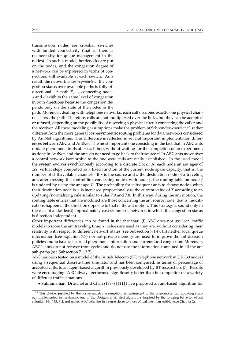
246 7. ACO ALGORITHMS FOR ADAPTIVE ROUTING
transmission nodes are crossbar switches
with limited connectivity (that is, there is
no necessity for queue management in the
nodes). In such a model, bottlenecks are put
on the nodes, and the congestion degree of
a network can be expressed in terms of con-
nections still available at each switch. As a
result, the network is cost-symmetric: the con-
gestion status over available paths is fully bi-
directional. A path Ps→d connecting nodes
s and d exhibits the same level of congestion
in both directions because the congestion de-
pends only on the state of the nodes in the
path. Moreover, dealing with telephone networks, each call occupies exactly one physical chan-
nel across the path. Therefore, calls are not multiplexed over the links, but they can be accepted
or refused, depending on the possibility of reserving a physical circuit connecting the caller and
the receiver. All these modeling assumptions make the problem of Schoonderwoerd et al. rather
different from the more general cost-asymmetric routing problems for data networks considered
by AntNet algorithms. This difference is reflected in several important implementation differ-
ences between ABC and AntNet. The most important one consisting in the fact that in ABC ants
update pheromone trails after each hop, without waiting for the completion of an experiment,
as done in AntNet, and the ants do not need to go back to their source.23 In ABC ants move over
a control network isomorphic to the one were calls are really established. In the used model
the system evolves synchronously according to a discrete clock. At each node an ant ages of
∆T virtual steps computed as a fixed function of the current node spare capacity, that is, the
number of still available channels. If s is the source and d the destination node of a traveling
ant, after crossing the control link connecting node i with node j, the routing table on node j
is updated by using the ant age T . The probability for subsequent ants to choose node i when
their destination node is s, is increased proportionally to the current value of T according to an
updating/normalizing rule similar to rules 7.9 and 7.8. In this way, during the ant motion, the
routing table entries that are modified are those concerning the ant source node, that is, modifi-
cations happen in the direction opposite to that of the ant motion. This strategy is sound only in
the case of an (at least) approximately cost-symmetric network, in which the congestion status
is direction-independent.
Other important differences can be found in the fact that: (i) ABC does not use local traffic
models to score the ant traveling time: T values are used as they are, without considering their
relativity with respect to different network states (see Subsection 7.1.4), (ii) neither local queue
information (see Equation 7.7) nor ant-private memory are used to improve the ant decision
policies and to balance learned pheromone information and current local congestion. Moreover,
ABC’s ants do not recover from cycles and do not use the information contained in all the ant
sub-paths (see Subsection 7.1.3.7).
ABC has been tested on a model of the British Telecom (BT) telephone network in UK (30 nodes)
using a sequential discrete time simulator and has been compared, in terms of percentage of
accepted calls, to an agent-based algorithm previously developed by BT researchers [7]. Results
were encouraging: ABC always performed significantly better than its competitor on a variety
of different traffic situations.
• Subramanian, Druschel and Chen (1997) [411] have proposed an ant-based algorithm for
23 This choice, justified by the cost-symmetry assumption, is reminiscent of the pheromone trail updating strat-egy implemented in ant-density, one of the Dorigo’s et al. first algorithms inspired by the foraging behavior of antcolonies [144, 135, 91], and makes ABC behavior in a sense closer to those of real ants than AntNet (see Chapter 2).
7.4 RELATED WORK ON ANT-INSPIRED ALGORITHMS FOR ROUTING 247
packet-switched networks. Their algorithm is a straightforward extension of Schoonderwoerd
et al. system by the addition of so-called uniform ants, a very simple (but of quite questionable
efficacy) exploration mechanism: ants just wonder around without a precise destination and
select their next hop according to a uniform random rule. While regular ants update the routing
tables forward, in the direction of their destination, uniform ants update in the reverse direction,
that is, toward the nodes they come from. Both the two types of ants update the routing tables
according to a not well specified path cost, which is the sum of the costs associated to each
one of the links belonging to the path followed so far. The mechanism of the uniform ant is
intended to avoid a rapid sub-optimal convergence of the algorithm and help to find new paths
in case of link/node failure (the algorithm is explicitly aimed at scenarios involving frequent
topological modifications). A major limitation of the approach consists in the fact that, although
the algorithm they propose is based on the same cost-symmetry hypothesis as ABC, they apply
it to packet-switched networks where this requirement is seldom met. On the other hand, the
pheromone updating of the uniform ants, since it happens in the reverse direction, does not
require the assumption of cost-symmetry, but it is however prone to efficiency problems since
the followed paths from one node to another are expected to be highly sub-optimal due to the
uniform random selection rule.
• Bonabeau, Henaux, Guerin, Snyers, Kuntz and Theraulaz (1998) [50] have improved ABC
by the introduction of a mechanism based on dynamic programming ideas. Pheromone values
along an ant path are updated not only with respect to the ant’s origin node as in ABC, but also
with respect to all the other intermediate nodes between the origin and the ant current node.
A similar mechanism, as discussed in depth in Subsection 7.1.3.7, was earlier implemented in
AntNet since its first draft version [116]. The difference between the AntNet’s and Bonabeau’s et
al. updating strategy lies in the fact that AntNet does not necessarily updates all the sub-paths
of a path, but only those which appear to carry reliable or competitive information. The fact that
a straight application of the Bellman’s principle is not free from problems has been discussed in
Subsection 7.1.3.7.
• Van der Put and Rothkrantz (1998, 1999) [426, 427] designed ABC-backward, an extension
of the ABC algorithm based on the AntNet strategy. Accordingly, ABC-backward is applicable
to cost-asymmetric networks, but, ultimately, the algorithm results to be identical to AntNet
with some, rather questionable simplifications directly inherited from the ABC settings. The
authors use the same forward-backward mechanism used in AntNet: Forward ants, while mov-
ing from the source to the destination node, collect information on the status of the network,
and backward ants use this information to update the routing tables of the visited nodes during
their journey back from the destination to the source node. In ABC-backward, backward ants
update the routing tables using an updating formula identical to that used in ABC, except for
the fact that the ants’ age is replaced by the trip times experienced by the ants in their forward
journey. The authors have shown experimentally that ABC-backward has a better performance
than ABC on both cost-symmetric (because backward ants can avoid depositing information on
cycles) and cost-asymmetric networks. ABC-backward has been applied to a fax distribution
problem proposed by the Dutch largest telephone company (KPN Telecom).
•White, Pagurek and Oppacher (1998) [445, 446] use an ACO algorithm for unicast and mul-
ticast routing in connection-oriented networks. The algorithm, called ASGA, follows a scheme
very similar to that of Ant System (see Section 4.2) which was designed for TSPs. On the other
hand, the TSP is a minimum cost path problem with the addition of the Hamiltonian constraint.
Therefore, it can be seen in the terms of a constrained routing problem. In this perspective, the
authors added some additional components to Ant System to account for the fact that they were
dealing with routing and not anymore with TSP. In particular, they have used the same forward-
backwardmechanism of AntNet, combined with a mechanisms very similar to that envisaged in
ACR for supporting the setup phase of a QoS or connection-oriented application and for main-
248 7. ACO ALGORITHMS FOR ADAPTIVE ROUTING
taining it. The major difference with AntNet lies in the fact that the authors apply the same
selection and updating formulae used in Ant System. In practice, Equation 7.7 is replaced by
one in which the terms are multiplied instead of being summed, and the l term is replaced by a
not clearly specified link cost. Equations 7.9 and 7.8 are replaced by exponential averages. From
the source node of each incoming connection, a group of ants is launched to search for a path. At
the beginning of the trip each ant k sets an internal path cost variable Ck to 0, and after each link
crossing the internal path cost is incremented by the current link cost lij : Ck ← Ck + lij . When
arrived at destination, the ant moves backward to its source node and at each node uses a simple
additive rule, similar to that of AntNet, to compute the equivalent of the AntNet’s T value: T
becomes equal to Ck, which is the sum of all the previously encountered costs. When all the
spooled ants come back at the source node, a simple local daemon algorithm decides whether a
path should be allocated for the session, based on the percentage of ants that followed a same
path. Moreover, during all the connection lifetime, the local daemon launches and coordinates
exploring ants to re-route the connection paths in case of network congestion or failures. A ge-
netic algorithm [202, 226] is used online to evolve two critical parameters (the equivalent of α in
Equation 7.7) that regulate the behavior of the transition rule formula (the name ASGA precisely
comes from this mechanism: ant-system plus genetic algorithm). Some preliminary results were
obtained testing the algorithm on several networks and using several link cost functions. Results
are promising: the algorithm is able to compute shortest paths and the genetic adaptation of the
rule parameters seems to improve considerably the algorithm’s performance.
Actually the same authors have published several other short conference papers on ant, swarm,
multi-agent systems for network management and control. Most of them mix the above mecha-
nisms and concepts with other similar flavors, therefore they are not further mentioned here.
•Heusse, Snyers, Guerin and Kuntz (1998) [224] developed a new algorithm for general cost-
asymmetric networks, called Co-operative Asymmetric Forward (CAF). CAF, even if still grounded
on the ACO framework, introduces some new ideas to exploit the advantages of an online step-
by-step pheromone updating scheme, as that used in ABC, in addition to the forward-backward
model of AntNet. In ABC the step-by-step updating strategy was made possible by the as-
sumptions of cost-symmetry, in CAF this assumption is relaxed, but it is still possible to use
step-by-step updates. In fact, each data packet, after going from node i to node j, releases on
node j the information cij about the sum of the waiting and crossing times experienced from
node i. This information can be used as an estimate of the traveling time to go from i to j. An
ant As→d hopping from j to i reads the cij information in j and moves it to i, where it is used
to update the estimate for the time to travel from i to j, and, accordingly, for the total traveling
time Ti→d′ from i to all the nodes s′ visited by the ant during its journey from s. In this way the
routing tables in the opposite direction of the ant motion can be updated online step-by-step.
Clearly, in order to work properly, the system requires that an “updating ant” would arrive in
coincidence or with a negligible time shift with respect to the moment the “information ant” de-
posited the information cij . The algorithm’s authors tested CAF under some static and dynamic
conditions, using the average number of packets waiting in the queues and the average packet
delay as performance measures. They compared CAF to an algorithm very similar to an earlier
version of AntNet. Results were encouraging and under all the test situations CAF performed
better than its competitors.
• The CAFmechanism is quite general and could be straightforwardly incorporated inAntNet
and AntNet-FA. Actually, Doi and Yamamura (2000, 2002) [133, 134] make use of a similar strat-
egy in their BntNetL algorithm. BntNetL has been designed as a supposed improvement over
AntNet-FA. Supposed because the authors misunderstood some of the behaviors of AntNet-FA
and then tried to devise some additional heuristics to “correct” them. For instance, they have
asserted that AntNet’s selection rule could get “locked” if one entry in the routing table would
reach the limit value of 1, but actually this is not the case, because AntNet-FA makes use of the
7.4 RELATED WORK ON ANT-INSPIRED ALGORITHMS FOR ROUTING 249
selection rule of Equation 7.7 which weights both the entries in the routing table and the current
status of the link queues. BntNetL has been compared to AntNet-FA on a restricted set of sim-
ulated situations. BntNetL and AntNet-FA (actually, a version of AntNet-FA containing some
incorrectly interpreted parts), showed more or less similar performance.
• On a similar stream of misleading interpretations of AntNet is the work of Oida and
Kataoka (1999) [337]. These authors, for some reasons, decided to work on improving the very
first draft version of AntNet [116], in which the status of the data link queues was not used,
such that the above mentioned “lock” mechanism could actually happen. To avoid this fact,
Oida and Kataoka have added some simple adaptive mechanisms to the routing table updat-
ing rule. Their algorithms, DCY-AntNet and NFB-Ants, once compared to the early version of
AntNet [116] performed much better under the challenging considered situations. Actually, the
mechanisms proposed by Oida and Kataoka could be also of some usefulness in AntNet-FA and
ACR, but their efficacy should be anyhow tested more carefully.
• The same Oida, but this time in collaboration with Sekido (1999, 2000) [339, 338], also
added some functionalities to the basic behavior of AntNet to make it suitable to work in a
QoS environment with constraints on the bandwidth and the number of hops. In particular,
in their algorithm Agent-based Routing System (ARS), they make the forward ants moving in a
“virtually constrained network” in order to support several classes of bandwidth requirements
(e.g., similarly to the DiffServ model [440]). The probability of a forward ant of choosing a link is
made depending not only on the values in the routing table but also on the level of the already
reserved bandwidth, and for each class of service in terms of bandwidth there is a different
colony of ants. All the ants of a colony only use those links whose the unreserved bandwidth
resources are not less than the value of the bandwidth constraint assigned to the colony. If
almost all bandwidth had already been reserved then the probability is accordingly made very
low. Similarly, if the number of executed hops is already too large and/or none of the outgoing
links has still much free bandwidth, then the forward ant terminates its journey. Interestingly,
these heuristics can be readily seen as the direct transposition of the basic AntNet’s mechanisms
in a QoS context. In fact, the heuristic taking into account the available bandwidth to assign
the link probabilities is equivalent to the AntNet’s heuristic that takes into account the current
number of bits waiting on the link queue. While the mechanisms for the ant self-termination
had already been implemented in AntNet by using the TTL parameter to remove those ants that
are trying to build a likely very bad path.
• Using the same concepts (stigmergy, ants, pheromone, multi-agency) underlying ACO but
not being explicitly inspired byACO, Fennet andHassas (2000) [166, 167] developed amodel of a
multi-agent system for multiple criteria balancing on a network of processors. It has been tested
on a some rather simple simulated situations. In their system ants move among the processing
units, perceiving local artificial pheromone fields that are emitted by the units and that encode
some useful information about the criteria to optimize. While the description that the authors
give of the actions and of the tasks is quite vague and not not well defined, it is interesting
to mention here that they use a terminology that reminds that of ACR: a distinction is made
between static and mobile agents interacting together, while the mobile agents are also seen as
sensory and effector agents for user applications.
• Baran and Sosa (2000) [13] have proposed several supposed improvements over AntNet:
(i) routing tables are initialized more efficiently by taking into account knowledge about the
neighbors, such that ants searching for destinations coinciding with one of the neighbors are not
actually generated, (ii) link and node failures are explicitly taken into account: after a link fail-
ure, the related pheromone entries are explicitly set to zero, (iii) with some small probability ants
can also issue a random uniform selection among the available alternatives in order to suppos-
edly reduce the (in)famous locking problem that has been repeatedly and incorrectly attributed
to AntNet, (iv) ants make greedy deterministic decisions instead of random proportional ones
250 7. ACO ALGORITHMS FOR ADAPTIVE ROUTING
(with the clear risk of incurring in very long lived loops and at the same time cutting off neces-
sary exploration),(v) the number of ants living in the network is arbitrarily limited to four times
the number of links (it is however not clear why this number and also how the number of active
ants can be actually determined given the fully distributed characteristics of the problem).
• Michalareas and Sacks (2001) [314] have studied the performance of an AntNet version
that makes use of deterministic greedy choices and of no link queue heuristic with respect to
that of an OSPF-like algorithm. The authors have considered three small topologies (tree, ring
and grid-like) and uniform FTP traffic using TCP Tahoe. According to the their results, at steady
state both the algorithms show equivalent performance. The same authors have implemented a
hybrid between their AntNet and ABC for the management of the routing in multi-constrained
QoS networks [315, 314]. They have considered an IP network offering soft-QoS service with
two constraints: on the end-to-end delay and on the available bandwidth. The proposed algo-
rithm makes use of two types of ant agents, one for each QoS constraint. The ants dealing with
the delay constraint are the same as in their previous version of AntNet, since AntNet’s ants
precisely try to minimize end-to-end delays. On the other hand, the bandwidth constraint is
dealt with ants that are artificially delayed at the nodes, as in ABC, proportionally to the occu-
pied link bandwidth as measured by a local exponential average of the link utilization. In this
way, their virtual delay bring a measure of the available bandwidth along the path. Experiments
conducted on the same traffic types and networks of the previously mentioned work show that
the AntNet-like algorithm performs similarly to an OSPF-like one, but scales much better with
the increasing of the load.
• In [378] (2001), Sandalidis, Mavromoustakis, and Stavroulakis have studied the perfor-
mance of Schoonderwoerd et al.’s ABC using a different network and considering some addi-
tional variables to monitor ants behavior. Their study confirms the earlier results for ABC. In a
more recent work [379] (2004), the same authors have developed a new version of ABC which
makes use of the notions of probabilistic routing of the phone calls and of anti-pheromone. When
an ant arrives at a node with an age larger than that currently recorded on the node, pheromone
is decreased instead of being increased. The performance of the new algorithm is compared to
that of ABC for a topology of 25 nodes and have shown a certain degree of improvement over it.
• Jain (2002) [234] has compared AntNet to a link-state protocol using the well known net-
work simulator ns-2. The author has implemented a version of AntNet very similar to that
of Michalareas and Sacks and has made use of greedy deterministic forwarding for data pack-
ets (the link with the highest probability is deterministically chosen), such that the algorithm
turned into a single-path one. Experiments were run on a small grid network and on the same
networks that have been used in the next chapter for AntNet experiments, but using different
traffic patterns. The experiments show that under light traffic conditions the two considered
algorithm behave similarly, but on the other hand the single-path AntNet algorithm can adapt
to new situations much quicker and much better.
•Kassabalidis, El-Sharkawi, Marks II, Arabshahi, and Gray (2002) [244] have proposed amod-
ification of AntNet based on the organization of the network in clusters and on the use ofmultiple
colonies. The network is first partitioned into clusters of nodes which are defined by running a
centralized k-means algorithm using as a metric the geographic location of the nodes (e.g., clus-
ters can be easily seen in the terms of Autonomous Systems in the Internet). Once the clustering
is realized, intra- and inter-clustering route discovery and maintenance is realized by two differ-
ent types of ants, and separate routing tables are hold at the nodes for intra- and inter-clustering
routing. In this way, the number of ants that have to be sent is in principle reduced, since every
node needs to hold a route only to each node in the same cluster it belongs to and to each other
cluster, and not to all the other nodes in the network (see also the discussion in Subsection 7.1.3.1
about the assumption of adopting a flat topological organization in AntNet). The authors pro-
pose also other minor modifications that are more simplifications of the AntNet’s mechanisms
7.4 RELATED WORK ON ANT-INSPIRED ALGORITHMS FOR ROUTING 251
more than real improvements. In particular, again, the authors have misunderstood AntNet’s
behavior, and affirm that in AntNet data packets are routed deterministically according to the
link with the highest probability (while a whole section is specifically devoted to this issue in
the main AntNet paper [120, Pages 352–353]). Their AntNet-derived algorithm, Adaptive-SDR,
was compared for two test networks of 16 and 49 nodes respectively to their single-path imple-
mentation of AntNet and to OSPF and RIP. The ns-2 simulator has been used. While AntNet,
OSPF, and RIP show similar performance, Adaptive-SDR shows much better results for both
throughput and average delay.
The same authors have also realized a short review on so-called swarm intelligence (in prac-
tice, ACO) algorithms for routing in networks [245]. Moreover, in [243] they have also discussed
the conditions for the applicability of AntNet-like algorithms to wireless networks, like satellite
and sensor networks. In particular, they have pointed out the importance of energy and radio
propagation issues, and have proposed some possible ways of incorporating these aspects in the
mechanisms used to search and score a path.
• Sim and Sun (2003) [390] have made a quite detailed review paper on ACO approaches
for routing and load balancing, focusing in particular on discussing the issue of the different
methods (for both static and dynamic problems) devised to avoid early convergence in the
pheromone tables (also previously indicated as stagnation or locked decisions). In the same
paper the authors propose an ACO approach, named MACO, based on multiple colonies for
load balancing tasks in connection-oriented networks. The idea is to use multiple colonies and
pheromone repulsion among colonies in order to find good disjoint path to allocate the traf-
fic sessions: at setup time of a traffic session multiple (two in the example reported in the
paper) colonies are generated and concurrently search for feasible paths. The issue of how
many colonies should be generated in not considered. Differently from what is claimed in
the paper, AntNet and AntNet-FA, with their stochastic data spreading, comes with a built-
in way of providing load balancing. However, the use of pheromone repulsion in order to favor
the exploration of disjoint paths appears as promising and it has been already used also by
Navarro Varela and Sinclair (1999) [333] to solve (static) problems of virtual wavelength path
routing and wavelength allocations. For this class of problems the challenge consists in allocat-
ing a minimum number of wavelengths for each link by evenly distributing the wavelengths
over the different links, while at the same time minimizing the number of hops for each path.
Pheromone repulsion is used precisely to favor the even distribution of the wavelengths.
• Tadrus and Bai (2003) [416] have implemented the QColony algorithm for QoS routing.
QColony is based on AntNet but contains a number of new features specific for QoS, such that
it is more correct to see it as an interesting example of ACR. In QColony each node contains
several QoS pheromone tables, with each table used to route ants associated to a different QoS
requirement. Each QoS table is associated to a range of continuous bandwidth constraints (i.e.,
each QoS table is related to one class of service in terms of provided range of bandwidth). QoS
sessions ask for a class of service in terms of acceptable range of bandwidth andmaximum num-
ber of hops. The QoS tables are built by the ants according to several proactive and on-demand
schemes, and are used by the ants to search for feasible QoS paths at the setup time of a new ses-
sion. The system comprises several classes of ant agents, each class has a different priority and
deals with a different task: search for best-effort paths, search for a QoS-feasible path at setup
time, retry of the search in case of failure of the first search attempt, allocation/deallocation
of resources, search for alternative paths to be used by the QoS sessions in case of link/node
failures. All the ants update the QoS tables, but with a strength which is proportional to their
priority and age. QColony shares several similarities with AntNet+SELA. In fact, both: make
use of different agents for the different tasks, search for a QoS-feasible path at setup time by us-
ing ants, send per-session ants (so-called soldier ants in the case of QColony) in order to provide
the QoS session with a bundle of paths to deal with possible failure situations, try to optimize
252 7. ACO ALGORITHMS FOR ADAPTIVE ROUTING
also the number of hops of the used paths. However, important differences also exist between
the two algorithms. In particular, one of the claims of QColony consists precisely in the fact
that purely local information is used at the nodes, while in the case of AntNet+SELA the node
manager issues its decisions on the basis of an OSPF-like topological description of the whole
network. The QColony’s design is quite interesting, since it is another crystalline example of
how different types of agents and on-demand/proactive generation strategies are jointly neces-
sary in order to effectively deal with complex routing tasks. The performance of QColony has
been compared to that of ARS and to the selective flooding algorithm described in [80]. For
the considered scenarios (three networks up to 35 nodes, and 10 ranges of bandwidth) QColony
has shown performance comparable to the competitors for small networks and mild traffic, and
much better performance for the larger networks and heavy traffic loads.
Other work in the domain of QoS is that of Subing and Zemin (2001) [410] and Carrillo et al.
(2003) [73], that suggest algorithms similar to QColony in the sense of using ants at setup time
and multiple QoS tables, but the structure of their algorithms is simpler and has less compo-
nents than that of QColony. The same authors of [73] have also made a preliminary theoretical
study on the general scalability of AntNet, showing the expected good level of scalability of the
approach [73].
•Other implementations of both the ACO and AntNet paradigms are the works of: Gallego-
Schmid (1999) [181], who implemented a minor modification of AntNet in the general perspec-
tive of using it for network management, and Zhong (2002) [452], which is the first who has
considered the issue of security when using AntNet, an issue that has been also pointed out
when ACR has been discussed, emphasizing the fact that ant agents should not be allowed to
directly modify the routing tables. The use of key certificates and ant identifiers are proposed as
a way to overcome to possible armful situations like: (i) generation of bogus backward ants in
order to promote/avoid a specific route, (ii) dropping ant agents in order to not allow them to
further update routing tables and/or find a path through the current node, (iii) tampering the
backward ants information in order to generate wrong routing paths.
Wireless and mobile ad hoc networks
• Matsuo and Mori (2001) [302] have proposed Accelerated Ants Routing, which is an extension
to MANETs of the ideas of Subramanian et al. [411]. They add the rule that uniform ants do not
return to an already visited node, and make these ants to hold the history about the n last visited
nodes. In this way, routing information can be updated not only toward the source, but all the
intermediate nodes. The algorithm heavily rely on the uniform ants, and no on-demand actions
are taken. It has been compared for a small 10 nodes network to Q-routing, dual Q-routing [264],
and to the original algorithm making use of uniform ants, showing better performance than the
competitors. In a later paper [178] the algorithmwas tested in a 56 node network, and compared
also to AntNet, again showing better performance and faster convergence.
• Camara and Loureiro (2001) [69, 68] describe a location-based algorithm which makes use
of ant agents to collect and disseminate routing information in MANETs. Every node keeps in a
routing table location information of all the other nodes, and routing paths are calculated with a
shortest path algorithm. To keep the tables up-to-date, information is exchanged locally among
neighbors, and globally by sending ants to nodes further away. In practice, ants implement
an efficient form of flooding. The algorithm is compared to another popular location-based
algorithm, LAR [255] and shows less overhead and comparable performance.
• Sigel, Denby, and Hearat-Mascle (2002) [389] have applied a straightforward modification
(and simplification) of AntNet to the problem of adaptive routing in the LEO satellite network.
Some experimental results from simulations are discussed taking into account some possibly
realistic traffic patterns in terms of both voice and data telecommunication. The algorithm is

7.4 RELATED WORK ON ANT-INSPIRED ALGORITHMS FOR ROUTING 253
compared to more a classical routing algorithms such as SPF (see next chapter), as well as to
an ”ideal” realization of it aimed at providing a kind of performance upper bound. Overall,
the performance of the proposed algorithm is near-optimal and much better than that of SPF,
especially for high non-bursty traffics.
• Gunes et al. (2002) [210, 211] introduced Ant-Colony-Based Routing Algorithm (ARA), which
does not differ much from other popular MANET algorithms like AODV. In fact, it works in a
purely on-demandway, with both the forward and backward ants setting up the paths about the
node they are coming from. Also data packets do the same, reducing in this way the node for
sending more ants. The reported performance was slightly better than that of AODV but worse
than that of DSR [236] in highly dynamic environments.
•Marwaha et al. (2002) [301] have proposedAnt-AODV, an hybrid algorithm combining ants
with the basic AODV behavior. A certain number of ants keeps going around the network in
a more or less random manner, keeping track of the last n visited nodes and when they arrive
at a node they update its routing table. The behavior of the algorithm is like AODV, but the
presence of the ants is supposed to boost AODV’s performance. In fact, they proactively refresh
routing tables, increasing the chance that either the node will have a route available or one
of its neighbors has. Moreover, ants can discover better paths than those currently in use by
AODV and the paths can be rerouted. According to the reported simulation studies, Ant-AODV
performs usually better than the simple ant-based algorithm or AODV separately.
• In [14] Baras and Mehta (2003) propose two algorithms for MANETs. The first is very sim-
ilar to AntNet: it is in fact purely proactive, trying to maintain pheromone entries for all the
destinations. It differs from AntNet because of data packets that are routed deterministically
and ants taking also random uniform decisions for the purpose of unbiased exploration. The
algorithm does not work very well, due to the large amount of routing overhead, and the ineffi-
cient route discovery. The second version of the algorithm, called Probabilistic Emergent Routing
Algorithm (PERA), is much closer to AODV. In fact, the algorithm becomes purely reactive: ants
are only sent out when a route is needed. Also, they are now broadcast instead of being unicast
to a certain destination. In this way, the forward ants are in practice identical to route request
messages in AODV and DSR. The only difference stays in the fact that multiple routes are set
up, but actually only the one with the highest probability is actually used by data, with the
other being available for quick recovery from link failures. The performance of the algorithm is
comparable to that of AODV.
• In [221], Heissenbuttel and Braun (2003) describe an ant-based algorithm for large scale
MANETs. The algorithm is quite complicate and makes use of geographical partitioning of the
node area. It shares some resemblance with the Terminode project [40, 39].
254 7. ACO ALGORITHMS FOR ADAPTIVE ROUTING
7.5 Summary
In this chapter four novel ACO algorithms for adaptive routing in telecommunication networks,
AntNet, AntNet-FA, AntHocNet, and AntNet+SELA, have been described and throughly dis-
cussed. These algorithms cover a wide range of possible network scenarios. Experimental result
are be reported in the next chapter, and only for the first three of them.
In addition to these algorithms, in this chapter we also introduced ACR, a high-level dis-
tributed control framework that specializes the general ACO’s ideas to the domain of network
routing and at the same time provides a generalization of these same ideas in the direction of
integrating explicit learning components into the design of ACO algorithms.
AntNet, which was chronologically the first of these algorithms to be developed, is a traffic-
adaptive multipath routing algorithm for best-effort datagram networks. It makes use of a strat-
egy based on:(i) ant-like mobile agents repeatedly and concurrently sampling paths between
assigned source and destination nodes, (ii) stochastic routing of data according to the local
pheromone values, with automatic load balancing and multipath routing effects, (iii) informa-
tion from both pheromone values (resulting from collective ant learning) and current status of
the local link queues (current congestion at the node) to take balanced ant routing decisions, (iv)
adaptive statistical models to track significant changes in the estimate end-to-end delays of the
sampled paths. The basic characteristics of the routing delivered by AntNet (traffic-adaptive,
and multipath), and the strategies adopted to obtain these behaviors (active sampling by mobile
agents, stochastic routing, Monte Carlo learning, use of local queues information) are in some
sense conserved also in all the other algorithms. They can be seen as their true fingerprints.
Moreover, we discussed in this and in the previous chapter why these characteristics and strate-
gies have to be seen as innovative with respect to those of popular routing algorithms.
AntNet-FA is an improvement over AntNet in which both backward and forward ants make
use of high priority queues. AntNet-FA allows prompter reactions and always makes use of
information more up-to-date with respect to AntNet. AntNet-FA is expected to always perform
equally or better than AntNet. This will be confirmed by the experimental results reported in
the next chapter.
ACR introduces a hierarchical organization into the previous schemes, with node managers
that are fully autonomic learning agents, and mobile ant-like agents that are under the direct
control of the node managers and serve for the purpose of non-local discovering andmonitoring
of useful information. Even if all the ACO routing algorithms described in this thesis can be seen
as instances of the ACR framework, the purpose of defining ACR is more ambitious than a pure
generalization of the ACO design guidelines for the specific case of network problems. ACR
defines the general architecture of a multi-agent society based on the integration of the ACO’s
philosophy with ideas from the domain of reinforcement learning, with the aim of providing a
framework of reference for the design and implementation of fully autonomic routing systems
in the same spirit as described in more general terms in [250] (fully distributed systems able to
globally self-govern through self-tuning, self-optimization, self-management, . . . , of the single
autonomic unit that socially interacts with all the other units). ACR points out the critical issues
of the scheduling of the ant-like agents, the definition of their characteristics, and the ability to
deal effectively with a range of different possible event (such that some diversity is necessary
into the population of the ant-like agents).
In order to show how these ACR issues can be (partly) dealt with, two more novel routing
algorithms have been described: AntNet+SELA, for QoS routing inATMnetworks, andAntHoc-
Net, for best-effort routing in mobile ad hoc networks. The purpose of introducing these two
additional algorithmswas twofold: from one hand they addressmore complex routing problems
than those considered by AntNet and AntNet-FA, such that that they are practical examples of
7.5 SUMMARY 255
how to deal with the issues of ant scheduling, diversity, response to several different high-level
events, and so on, raised up in ACR. So, they can be seen as practical instances of ACR. On the
other hand, with AntNet+SELA and AntHocNet in addition to AntNet and AntNet-FA, we have
covered the majority of the routing scenarios of practical interest.
In AntNet+SELA the node managers, that are directly responsible for both routing and ad-
mission decisions, are designed after the stochastic estimator learning automata (SELA) [430] used
in the SELA-routing distributed system [8]. They make use of several types of agents: (i) mobile
ant-like (perception) agents to collect non-local information, and that are generated according
to both on-demand (at session setup time) and proactive generation schemes, and (ii) mobile
effectors agents used to tear down paths and to gather specific information about traffic pro-
files of running applications. The different perception agents are designed after the AntNet-FA
ants, however, they are generated with different parameters in order to have different behaviors
according to the different task they are involved in.
AntHocNet is a reactive-proactive multipath algorithm for routing in MANETs. Node man-
agers are not really learning agents as it was the case for AntNet+SELA, but rather finite state
machines responding more or less reactively to external events and generating the appropri-
ate action and type of ant-like agent. In particular, the design of AntHocNet features: reactive
agents to setup paths toward a previously unknown destination, per-session proactive gathering
of information, and agents for the explicit management of link failure situations (repair and noti-
fication to the neighbors). The fact that a strong reactive component is included in the algorithm
is partially due to the fact that in such highly dynamic environments it might be of questionable
utility to rely on approaches strongly based on detecting and learning environment’s regulari-
ties. Some level of learning and proactivity is expected to be of some usefulness, but at the same
time the core strategy is expected to be a reactive one.
The chapter has also extensively reviewed related work in the domain of ant-inspired algo-
rithms for routing tasks. The review has pointed out the main different solutions proposed so
far, as well as has served to remark the interest that AntNet and, more in general, ACO ideas,
have aroused in the routing community.

256 7. ACO ALGORITHMS FOR ADAPTIVE ROUTING
CHAPTER 8
Experimental results for ACO
routing algorithms
This chapter is devoted to the presentation of extensive experimental results concerning AntNet,
AntNet-FA, and AntHocNet. The majority of the results concern AntNet and AntNet-FA and re-
fer to the case of best-effort routing in wired IP networks. As discussed in Subsection 7.1.1, failure
events are not taken into account, the focus being on the study of traffic-adaptiveness and on the
effective use of multiple paths. Some preliminary results concerning AntHocNet and routing
mobile ad hoc networks are also briefly reported. However, AntHocNet is still under develop-
ment and testing, such that these results must be considered as preliminary ones.
All the results refer to simulations. The algorithms have not been tested yet on real networks,
even if some explicit interest in this sense has been shown by some important network compa-
nies. Actually, a large part of the research in the field of networks is based on simulation studies,
due to the difficulties related to the use of effective mathematical tools to study the properties
of routing algorithms under realistic assumptions (e.g., see the extensive discussions in [325]).
The simulator that has been implemented and used for the experiments has the characteristics
discussed in Subsection 7.1.1.
Nomathematical proofs concerning the specific properties of the algorithms are provided. In
fact, a sound mathematical treatment for the non-stationary case would require the knowledge
of the dynamics of the input traffic processes, but this is precisely what is a priori not known. If
such knowledge is available, an optimal routing approach (Subsection 6.4.1) should be definitely
adopted (at least in the wired case, while the situation is way more complex in the wireless
and mobile case). Moreover, such dynamics should be representable in terms of low-variance
stationary stochastic processes to be amenable to effective mathematical analysis. On the other
hand, it is not immediately obvious which type of convergence or stability is appropriate to be
studied under conditions of non-stationarity.
Concerning convergence under conditions of traffic stationarity, the general proofs of con-
vergence provided for the more general ACO case by Stutzle and Dorigo [403] and Gutjahr [214,
215, 216] can intuitively guarantee that a basic form of an AntNet-like algorithm, will converge
to an optimal solution. Where the optimality must be intended in some sense in between the
optimal shortest path solution and the optimal routing solution. In fact, the optimization strat-
egy followed by AntNet and AntNet-FA can be situated in between the criteria used by these
two approaches. However, ACR algorithms are intended for traffic-adaptive routing. The case
of static or quasi-static traffic patterns is in a sense not of interest. Generic ACR algorithms are
not expected to be really competitive with more classical approaches for the static case. what
is termed batch Monte Carlo it can be expected to minimize the mean hypothetically available
training set. (p. 144)
The experimental results will show that under all the considered situations AntNet and
AntNet-FA clearly outperform all the considered five competitors, that include several traffic-
adaptive state-of-the-art algorithms. Tests have been run for a number of different traffic pat-
terns and for five different topologies (two real-world ones, two artificially designed ones, and
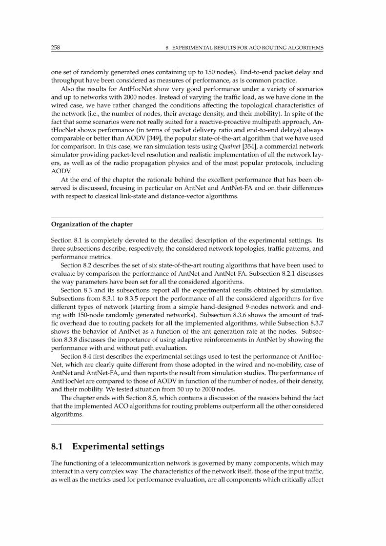
258 8. EXPERIMENTAL RESULTS FOR ACO ROUTING ALGORITHMS
one set of randomly generated ones containing up to 150 nodes). End-to-end packet delay and
throughput have been considered as measures of performance, as is common practice.
Also the results for AntHocNet show very good performance under a variety of scenarios
and up to networks with 2000 nodes. Instead of varying the traffic load, as we have done in the
wired case, we have rather changed the conditions affecting the topological characteristics of
the network (i.e., the number of nodes, their average density, and their mobility). In spite of the
fact that some scenarios were not really suited for a reactive-proactive multipath approach, An-
tHocNet shows performance (in terms of packet delivery ratio and end-to-end delays) always
comparable or better than AODV [349], the popular state-of-the-art algorithm that we have used
for comparison. In this case, we ran simulation tests using Qualnet [354], a commercial network
simulator providing packet-level resolution and realistic implementation of all the network lay-
ers, as well as of the radio propagation physics and of the most popular protocols, including
AODV.
At the end of the chapter the rationale behind the excellent performance that has been ob-
served is discussed, focusing in particular on AntNet and AntNet-FA and on their differences
with respect to classical link-state and distance-vector algorithms.
Organization of the chapter
Section 8.1 is completely devoted to the detailed description of the experimental settings. Its
three subsections describe, respectively, the considered network topologies, traffic patterns, and
performance metrics.
Section 8.2 describes the set of six state-of-the-art routing algorithms that have been used to
evaluate by comparison the performance of AntNet and AntNet-FA. Subsection 8.2.1 discusses
the way parameters have been set for all the considered algorithms.
Section 8.3 and its subsections report all the experimental results obtained by simulation.
Subsections from 8.3.1 to 8.3.5 report the performance of all the considered algorithms for five
different types of network (starting from a simple hand-designed 9-nodes network and end-
ing with 150-node randomly generated networks). Subsection 8.3.6 shows the amount of traf-
fic overhead due to routing packets for all the implemented algorithms, while Subsection 8.3.7
shows the behavior of AntNet as a function of the ant generation rate at the nodes. Subsec-
tion 8.3.8 discusses the importance of using adaptive reinforcements in AntNet by showing the
performance with and without path evaluation.
Section 8.4 first describes the experimental settings used to test the performance of AntHoc-
Net, which are clearly quite different from those adopted in the wired and no-mobility, case of
AntNet and AntNet-FA, and then reports the result from simulation studies. The performance of
AntHocNet are compared to those of AODV in function of the number of nodes, of their density,
and their mobility. We tested situation from 50 up to 2000 nodes.
The chapter ends with Section 8.5, which contains a discussion of the reasons behind the fact
that the implemented ACO algorithms for routing problems outperform all the other considered
algorithms.
8.1 Experimental settings
The functioning of a telecommunication network is governed by many components, which may
interact in a very complex way. The characteristics of the network itself, those of the input traffic,
as well as the metrics used for performance evaluation, are all components which critically affect
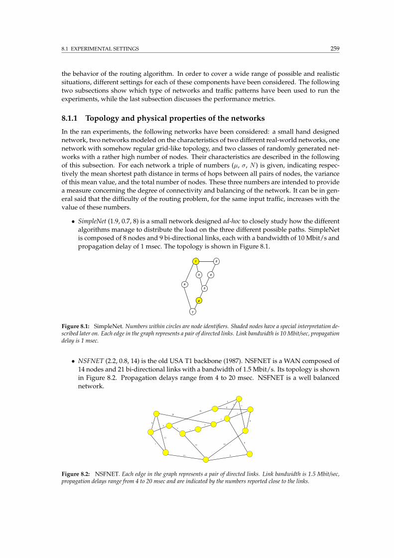
8.1 EXPERIMENTAL SETTINGS 259
the behavior of the routing algorithm. In order to cover a wide range of possible and realistic
situations, different settings for each of these components have been considered. The following
two subsections show which type of networks and traffic patterns have been used to run the
experiments, while the last subsection discusses the performance metrics.
8.1.1 Topology and physical properties of the networks
In the ran experiments, the following networks have been considered: a small hand designed
network, two networks modeled on the characteristics of two different real-world networks, one
network with somehow regular grid-like topology, and two classes of randomly generated net-
works with a rather high number of nodes. Their characteristics are described in the following
of this subsection. For each network a triple of numbers (µ, σ, N ) is given, indicating respec-
tively the mean shortest path distance in terms of hops between all pairs of nodes, the variance
of this mean value, and the total number of nodes. These three numbers are intended to provide
a measure concerning the degree of connectivity and balancing of the network. It can be in gen-
eral said that the difficulty of the routing problem, for the same input traffic, increases with the
value of these numbers.
• SimpleNet (1.9, 0.7, 8) is a small network designed ad-hoc to closely study how the different
algorithms manage to distribute the load on the three different possible paths. SimpleNet
is composed of 8 nodes and 9 bi-directional links, each with a bandwidth of 10 Mbit/s and
propagation delay of 1 msec. The topology is shown in Figure 8.1.
8
2
4
6
5
7
3
1
Figure 8.1: SimpleNet. Numbers within circles are node identifiers. Shaded nodes have a special interpretation de-scribed later on. Each edge in the graph represents a pair of directed links. Link bandwidth is 10Mbit/sec, propagationdelay is 1 msec.
• NSFNET (2.2, 0.8, 14) is the old USA T1 backbone (1987). NSFNET is a WAN composed of
14 nodes and 21 bi-directional links with a bandwidth of 1.5 Mbit/s. Its topology is shown
in Figure 8.2. Propagation delays range from 4 to 20 msec. NSFNET is a well balanced
network.
9
7
15 9
81411
13
9
20
16
5
7
47
7
77
8
5
7
Figure 8.2: NSFNET. Each edge in the graph represents a pair of directed links. Link bandwidth is 1.5 Mbit/sec,propagation delays range from 4 to 20 msec and are indicated by the numbers reported close to the links.
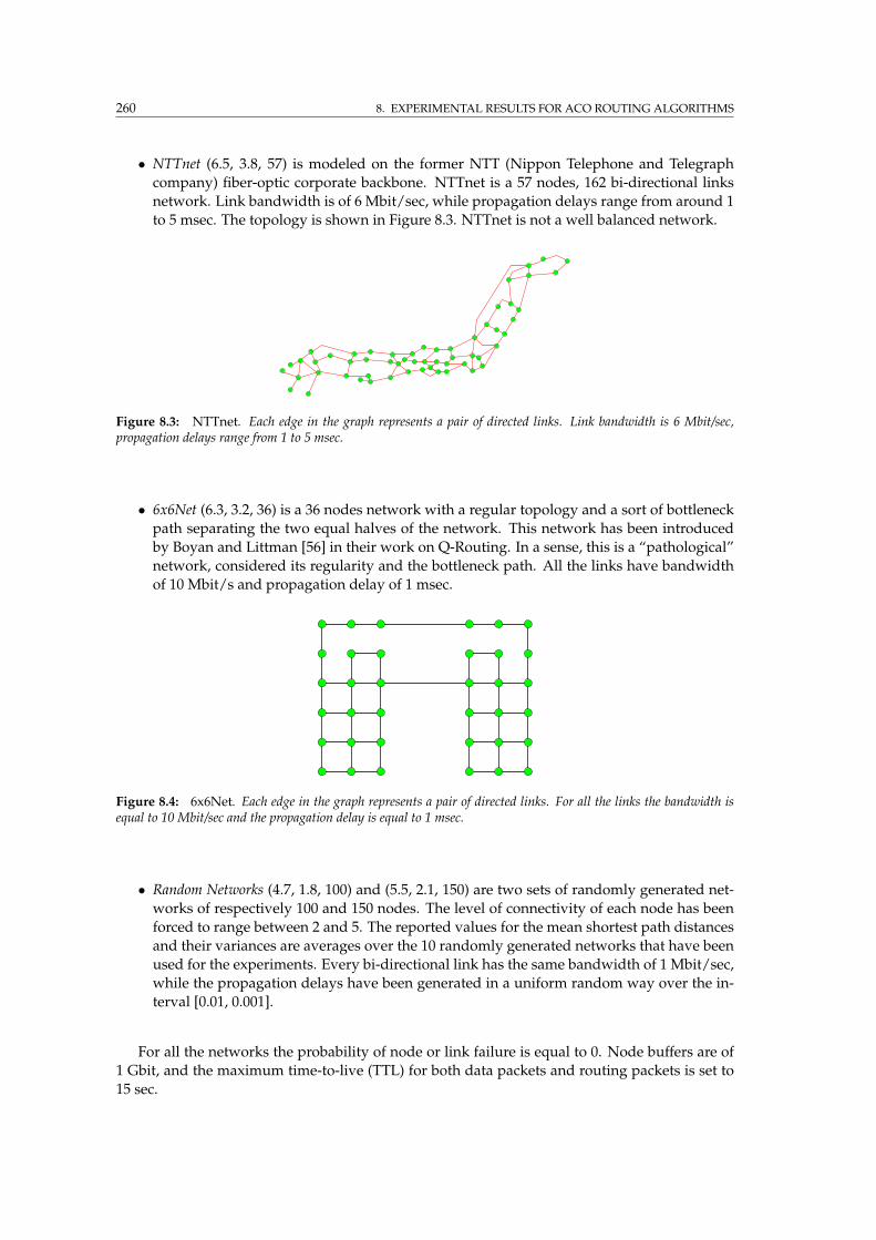
260 8. EXPERIMENTAL RESULTS FOR ACO ROUTING ALGORITHMS
• NTTnet (6.5, 3.8, 57) is modeled on the former NTT (Nippon Telephone and Telegraph
company) fiber-optic corporate backbone. NTTnet is a 57 nodes, 162 bi-directional links
network. Link bandwidth is of 6 Mbit/sec, while propagation delays range from around 1
to 5 msec. The topology is shown in Figure 8.3. NTTnet is not a well balanced network.
Figure 8.3: NTTnet. Each edge in the graph represents a pair of directed links. Link bandwidth is 6 Mbit/sec,propagation delays range from 1 to 5 msec.
• 6x6Net (6.3, 3.2, 36) is a 36 nodes network with a regular topology and a sort of bottleneck
path separating the two equal halves of the network. This network has been introduced
by Boyan and Littman [56] in their work on Q-Routing. In a sense, this is a “pathological”
network, considered its regularity and the bottleneck path. All the links have bandwidth
of 10 Mbit/s and propagation delay of 1 msec.
Figure 8.4: 6x6Net. Each edge in the graph represents a pair of directed links. For all the links the bandwidth isequal to 10 Mbit/sec and the propagation delay is equal to 1 msec.
• Random Networks (4.7, 1.8, 100) and (5.5, 2.1, 150) are two sets of randomly generated net-
works of respectively 100 and 150 nodes. The level of connectivity of each node has been
forced to range between 2 and 5. The reported values for the mean shortest path distances
and their variances are averages over the 10 randomly generated networks that have been
used for the experiments. Every bi-directional link has the same bandwidth of 1 Mbit/sec,
while the propagation delays have been generated in a uniform random way over the in-
terval [0.01, 0.001].
For all the networks the probability of node or link failure is equal to 0. Node buffers are of
1 Gbit, and the maximum time-to-live (TTL) for both data packets and routing packets is set to
15 sec.
8.1 EXPERIMENTAL SETTINGS 261
8.1.2 Traffic patterns
Traffic is defined in terms of open sessions between pairs of different nodes. Traffic patterns over
the whole network depend on the characteristics of each session and on their geographical and
temporal distribution.
Each single session is characterized by the number of transmitted packets and by the dis-
tribution of their sizes and inter-arrival times. Sessions over the network are characterized by
their geographical distribution and by their inter-arrival time. The geographical distribution is
controlled by the probability assigned to each node to be selected as a start- or end-point of a
session.
Arrival of new sessions at the nodes
The following three different types of basic processes have been used in the experiments to
regulate the arrival of new sessions at the nodes:
• Poisson (P): for each node an independent Poisson process regulates the arrival of new
sessions, i.e., sessions’ inter-arrival times are negative exponentially distributed.
• Fixed (F): at the beginning of the simulation an assigned number of sessions is set up at
each node, and they keep sending data for all the remainder of the simulation.
• Temporary Hot Spots (TMPHS): in this case some nodes act like temporary hot spots, that is,
they generate a heavy load of traffic but only for a short time interval.
Geographical distribution of traffic sessions
The geographical distribution of the active sessions all over the network is defined according to
one of the following three basic patterns:
• Uniform (U): the characteristics of the process that at each node is regulating the arrival of
new sessions are the same for all the nodes in the network.
• Random (R): the characteristics of the process that at each node is regulating the arrival of
new sessions are set up according to the same randomized procedure for all the network
nodes.
• Hot Spots (HS): some nodes act as hot spots, concentrating a high rate of input/output
traffic. In this case, a fixed number of sessions are opened from the hot spots toward all
the other nodes.
Complex traffic patterns have been obtained by combining in various ways the above basic
patterns for temporal and spatial distribution (e.g., F-CBR, UP, UP-HS). For example, UP traffic
means that for each node an identical Poisson process is regulating the arrival of new sessions,
while RP means that the Poisson process is different for each node and its characteristics are
drawn from a random distribution. UP-HS means that a Hot Spots traffic process is superim-
posed to a UP traffic, and so on.
Packet stream of traffic sessions
Concerning the characteristics of the bit stream generated by each session, two basic types have
been considered:
262 8. EXPERIMENTAL RESULTS FOR ACO ROUTING ALGORITHMS
• Constant Bit Rate (CBR): the per-session bit rate is kept constant. Examples of applications
of CBR streams are the voice signal in a telephone network, which is converted into a
stream of bits with a constant rate of 64 Kbit/sec, and the MPEG1 compression standard,
which converts a video signal into a stream of 1.5 Mbit/sec.
• Generic Variable Bit Rate (GVBR): the per-session generated bit rate is time varying. The
term GVBR is a broad generalization of the VBR term normally used to designate a bit
streamwith a variable bit rate but with known average characteristics and expected/admitted
fluctuations.1 Here, a GVBR session generates packets whose sizes and inter-arrival times
are variable and follow a negative exponential distribution. The information about these
characteristics is never directly used by the implemented routing algorithms.
The values used in the experiments to shape traffic patterns are values considered somehow
“reasonable” once the current network usage and computing power are taken into account. The
mean of the distribution of packet sizes has been set to 4096 bits in all the experiments.
8.1.3 Performance metrics
Results refer to measures of throughput, packet delays and network resources utilization. Results
for throughput are reported as average values without an associated measure of variance. The
inter-trial variability is in fact usually very low, just a few percent of the average value. Network
resource utilization is only considered with respect to the routing packets and is reported for
a single specific sample instance. Numerical results on packet delays are reported either by
displaying the whole empirical distribution or by using the statistic of the 90-th percentile. The
empirical distribution shows the complete picture of what happened during the observation
interval, but it might be difficult to compare two empirical distributions. On the contrary, the
90-th percentile allows to compactly compare the algorithms on the basis of the upper value of
delay they been have able to keep the 90% of the correctly delivered packets. In other works on
routing, the mean packet delay is often used as a sufficient statistics for packet delays. However,
the mean value is of doubtful significance. In fact, packet delays can spread over a wide range
of values. This is an intrinsic characteristics of data networks: end-to-end delays can range from
very low values for sessions open between adjacent nodes and connected by fast links, to much
higher values in the case of sessions involving nodes very far apart and possibly connected by
several slow links. According to this, in general, the empirical distribution of packet delays
cannot be meaningfully parametrized in terms of the mean and variance. This is why here the
display of the whole empirical distribution and/or the statistics of the 90-th percentile have been
used.
Most of the results will show little difference in throughput among the algorithms, while
more marked differences will concern end-to-end delays. This is also a consequence of the fact
that node buffers are quite large. Therefore, packets can accumulate long delays while suffering
little throughput loss due to dropping because of lack of buffer space (however, the 15 seconds
TTL put a limit on the maximum delay that a packet can experience). Some experiments con-
ducted with smaller buffers have confirmed the obtained results with differences more marked
for what concerns throughput.
1 The knowledge about the characteristics of the incoming CBR or VBR bit streams is of fundamental importance innetworks able to deliver QoS. It is on the basis of this knowledge that the network can accept/refuse the session requests,and, in case of acceptance, allocate/reserve necessary resources.
8.2 ROUTING ALGORITHMS USED FOR COMPARISON 263
8.2 Routing algorithms used for comparison
The performance of AntNet and AntNet-FA is compared to that of the following routing algo-
rithmswhich are taken as representative of the state-of-the-art in the fields of telecommunication
and machine learning for both the cases of static and adaptive algorithms.
OSPF (static, link-state): the algorithm considered here is a simplified implementation ofOSPF
[328], the most used Interior Gateway Protocol on the Internet (see Chapter 6). According
to the assumptions made for the communication network model as described in Subsec-
tion 7.1.1 (no failure situations or topological modifications), the routing protocol here
called OSPF does not mirror the real OSPF protocol in its details. It only retains some
basic features of OSPF. Link costs are statically assigned on the basis of the link physical
characteristics. Routing tables are set as the result of the shortest (minimum end-to-end
delay) path computation for a sample data packet of 512 bytes. This way of assigning link
costs penalizes the implemented version of OSPF with respect to the one used on real net-
works, where costs are set up by network administrators, who can use additional heuristic
and the on-field knowledge they have about local traffic workloads. Since no topological
alterations are considered, the periodically flooded link state advertising messages have
always the same contents. As a result, the routing tables do not change over time and the
algorithm is here labeled as “static”, while the real OSPF is a dynamic algorithm in the
sense specified in Subsection 6.2.2 (i.e., topology-adaptive).
SPF (adaptive, link-state): this algorithm is a sort of prototype of link-state algorithms with adap-
tive link costs. A similar algorithm was implemented in the second version of ARPANET
[304] and in its successive revisions [252] (see Section 6.5). The implementation consid-
ered here makes use of the same flooding algorithm used in the real implementation,
while link costs are assigned over a discrete scale of 20 values by using the ARPANET
hop-normalized-delay metric2 of Khanna and Zinky [252] and the the statistical window av-
erage method described in [386]. Link costs are computed as weighted averages between
short- and long-term real-valued statistics reflecting a cost measure (e.g., utilization, queu-
ing and/or transmission delay, etc.) over time intervals of assigned length. The resulting
cost values are then rescaled and saturated by a linear function in order to obtain a value
in the range 1, 2, 3, . . . , 20. We have tried also other discrete and real-valued metrics in
addition to the discretized hop-normalized-delay, but none of them was able to provide
better performance and stability than the hop-normalized-delay one. The reason might
be that using a discrete scale reduces the sensitivity of the algorithm but at the same time
reduces also undesirable oscillations.
BF (adaptive, distance-vector): is an implementation of the asynchronous distributed Bellman-Ford
algorithm [26] making use of adaptive cost metrics. The basic structure of the algorithm
is the same as described in Subsection 6.4.2.1, while link costs are calculated as in the SPF
case, that is, according to [386]. As discussed in Subsection 6.4.2.1, several enhanced ver-
sions of the basic Bellman-Ford algorithm can be found in the literature (e.g., the Merlin-
Segall [310] and the Extended Bellman-Ford [82]). However, these algorithmsmainly focus
on the problem of avoiding the counting to infinity, or, more in general, the slow conver-
gence recovering from a link failure. These algorithms try to optimize the time necessary
to spread the information about the link failure such that the risk of routing inconsisten-
cies is much reduced. On the other hand, concerning dynamic situations other than link
2 The transmitting nodemonitors the average packet delay d (queuing plus transmission time) and the average packettransmission time t over observation windows of assigned time length. From these measures, and assuming an M/M/1queue model [26], a cost measure for the link utilization is calculated as 1 − t/d.
264 8. EXPERIMENTAL RESULTS FOR ACO ROUTING ALGORITHMS
failures, their behavior is in general equivalent to that of the basic adaptive distributed
Bellman-Ford considered here.
Q-R (adaptive, distance-vector): this algorithm is a faithful implementation of theQ-Routing al-
gorithm proposed by Boyan and Littman [56]. The algorithm makes use of the Q-learning
[442] updating rule within a scheme which is an online version of the asynchronous dis-
tributed Bellman-Ford algorithm. Q-learning is a popular reinforcement learning algo-
rithm designed for solving Markov decision process without relying on the use of the
environment model. Q-Routing learns online the values Qk(d, n), which are estimates of
the time to reach node d from node k via the neighbor node n. The algorithm operates as
follows. Upon sending a packet P from node k to neighbor node n with destination d, a
back packet Pback is immediately generated from n to k. Pback carries: (i) the information
about the current estimate
Q∗n(d) = min
n′∈N (n)Qn(d, n
′)
held at node n about the best expected time-to-go for destination d, and (ii) the sum TPk→n
of the queuing and transmission time experienced by P to hop from k to n. The sum
Qk(d, n) = Q∗n(d) + TPk→n
is used to update the k’s Q-value for destination d and neighbor n:
∆Qk(d, n) = η(Qk(d, n)−Qk(d, n)), η ∈ (0, 1] .
Data packets are routed toward the neighbor currently associated to the Q∗ estimate. In
the BF scheme running averages for link costs are calculated locally and then broadcast at
somehow regular intervals to the neighbors, that, in turn use them to directly update their
time-to-go estimates. In the Q-routing scheme, local estimates are sent from one node to
another after each packet hop, and time-to-go estimates are updated not by direct value
replacement but rather using exponential averaging.
PQ-R (adaptive, distance-vector): this is the Predictive Q-Routing algorithm [84], which is an
extended and revised version of Q-Routing designed to possibly deal in a better way with
traffic variability. In Q-routing, the best link (i.e., the one with the lowest Qk(d, n)) is
always deterministically chosen by data packets. Therefore, a neighbor n which has has
been associated to a high value of Qk(d, n), for example because of a temporary high load
condition, will never be used again until all the other neighbors will be associated to a
worse, that is, higher, Q-value. To overcome this potential problem, PQ-R try to learn a
model, called the recovery rate, of the variation rate of the local link queues, and makes use
of it to probe also those links that, although do no have the lowest Qk(d, n), shows a high
recovery rate. The idea is to give a chance to those links that seem to have recovered from
that was only a temporary congestion.
Daemon (adaptive, centralized): this algorithm is defined to provide a measure of an empirical
upper bound on the achievable performance. It is a sort of ideal algorithm, in the sense that
in general it cannot be implemented in practice since is at the same time centralized and
makes use of a “daemon” able to instantaneously read the state of all the queues in the
network such that shortest path calculations can be done for each packet hop according to
the up-to-date overall network status. A more precise upper bound could have been de-
fined by assuming full knowledge on the input traffic processes and then calculating the
optimal routing solution. However, such solution would have required to choose traffic
patterns amenable to mathematical treatment, and would have ruled out the study of tem-
porary hot spots situations. On the other hand, the Daemon algorithm proposed here can

8.2 ROUTING ALGORITHMS USED FOR COMPARISON 265
be applied to any kind of traffic patterns and does not require any additional knowledge.
The algorithm works as follows.
Link costs are defined in terms of the depletion time of the corresponding queue (similarly
to the strategy adopted in AntNet-FA), and the daemon knows at any time the cost of all
the links in the network. In order to assign the next hop node, before each packet hop the
algorithm re-calculates the shortest path solution according to the current costs of all net-
work links. The next hop node is then chosen as the one along the current minimum cost
path. In a sense, Daemon behaves as an SPF making use of instantaneous and continuous
information flooding.
Links costs express the time necessary for a new packet of size sp to cross the link l given
the current queues:
Cl = dl +spbl
+ (1− α)qlbl
+ αqlbl,
where dl is the transmission delay for link l, bl is its bandwidth, ql is the current size (in bits)
of the queue of link l, and ql is an exponential average of the size of the same link queue. By
means of the weight factor α, a weighted average between ql and ql is in practice calculated
in order to take into account both the current and the previous level of congestion along
the link (the value of α has been set to 0.4 in all the ran experiments). Clearly, for each
recalculation of the shortest paths, the value of sp is set to zero for all links but the ones
connected to the node where the current packet to be routed is located at.
8.2.1 Parameter values
All the implemented algorithms depend on their own set of parameters. For all the algorithms
the size of their routing packets and the related elaboration time must be properly set. Settings
for these specific parameters are shown in Table 8.1.
Table 8.1: Characteristics of routing packets for the implemented algorithms, except for the Daemon algorithm,which does not generate routing packets. Nh is the incremental number of hops made by the forward ant, |Nn| is thenumber of neighbors of the generic node n, and N is the total number of network nodes.
AntNet AntNet-FA OSPF, SPF BF Q-R, PQ-R
Packet size (byte) 24 + 8Nh 24 + 4Nh 64 + 8|Nn| 24 + 12N 12Packet processing time (msec) 3 3 6 2 3
These parameters have been assigned on the basis of values used in previous simulation
works [5] and/or on the basis of heuristic evaluations taking into consideration information
encoding schemes and currently available computing power. The size for AntNet forward ants
has been determined as the same size of a BF packet plus 8 bytes for each hop to store the
information about the node address and the traveling time. In the case of AntNet-FA only 4
additional bytes are necessary for each hop.
Except for AntNet, the parameters specific to each algorithm have been assigned by using the
best settings available in the literature, and/or through a tuning process in order to obtain pos-
sibly better results. The length of the time interval between consecutive broadcasting of routing
information and the length of the time window to average the link costs are both set to the value
of 0.8 or 3 seconds, depending on the experiment, for SPF and BF. The same values have been set
to 30 seconds for OSPF. Link costs inside each time window are assigned as the weighted sum
between the arithmetic average computed over the window and an exponential average with
decay factor equal to 0.9. The obtained values are mapped on a scale of integer values ranging
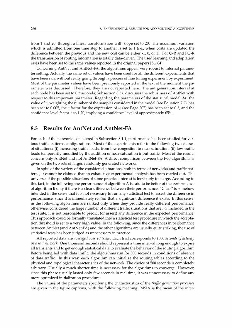
266 8. EXPERIMENTAL RESULTS FOR ACO ROUTING ALGORITHMS
from 1 and 20, through a linear transformation with slope set to 20. The maximum variation
which is admitted from one time step to another is set to 1 (i.e., when costs are updated the
difference between the previous and the new cost can be either -1, 0, or 1). For Q-R and PQ-R
the transmission of routing information is totally data-driven. The used learning and adaptation
rates have been set to the same values reported in the original papers [56, 84].
Concerning AntNet and AntNet-FA, the algorithms appear very robust to internal parame-
ter setting. Actually, the same set of values have been used for all the different experiments that
have been ran, without really going through a process of fine tuning experiment by experiment.
Most of the parameter values have been previously reported in the text at the moment the pa-
rameter was discussed. Therefore, they are not repeated here. The ant generation interval at
each node has been set to 0.3 seconds; Subsection 8.3.6 discusses the robustness of AntNet with
respect to this important parameter. Regarding the parameters of the statistical modelM: the
value of η, weighting the number of the samples considered in the model (see Equation 7.2), has
been set to 0.005, the c factor for the expression of w (see Page 207) has been set to 0.3, and the
confidence level factor z to 1.70, implying a confidence level of approximately 65%.
8.3 Results for AntNet and AntNet-FA
For each of the networks considered in Subsection 8.1.1, performance has been studied for var-
ious traffic patterns configurations. Most of the experiments refer to the following two classes
of situations: (i) increasing traffic loads, from low congestion to near-saturation, (ii) low traffic
loads temporarily modified by the addition of near-saturation input traffic. Most of the results
concern only AntNet and not AntNet-FA. A direct comparison between the two algorithms is
given on the two sets of larger, randomly generated networks.
In spite of the variety of the considered situations, both in terms of networks and traffic pat-
terns, it cannot be claimed that an exhaustive experimental analysis has been carried out. The
universe of the possible situations of some practical interest is inevitably too large. According to
this fact, in the following the performance of algorithm A is said to be better of the performance
of algorithm B only if there is a clear difference between their performance. “Clear” is somehow
intended in the sense that it is not necessary to run any statistical test to assert the difference in
performance, since it is immediately evident that a significant difference it exists. In this sense,
in the following algorithms are ranked only when they provide really different performance,
otherwise, considered the large number of different traffic situations that are not included in the
test suite, it is not reasonable to predict (or assert) any difference in the expected performance.
This approach could be formally translated into a statistical test procedure in which the accepta-
tion threshold is set to a very high value. In the following, since the differences in performance
between AntNet (and AntNet-FA) and the other algorithms are usually quite striking, the use of
statistical tests has been judged as unnecessary in practice.
All reported data are averaged over 10 trials. Each trial corresponds to 1000 seconds of activity
in a real network. One thousand seconds should represent a time interval long enough to expire
all transients and to get enough statistical data to evaluate the behavior of the routing algorithm.
Before being fed with data traffic, the algorithms run for 500 seconds in conditions of absence
of data traffic. In this way, each algorithm can initialize the routing tables according to the
physical and topological characteristics of the network. The choice of 500 seconds is completely
arbitrary. Usually a much shorter time is necessary for the algorithms to converge. However,
since this phase usually lasted only few seconds in real time, it was unnecessary to define any
more optimized initialization procedure.
The values of the parameters specifying the characteristics of the traffic generation processes
are given in the figure captions, with the following meaning: MSIA is the mean of the inter-
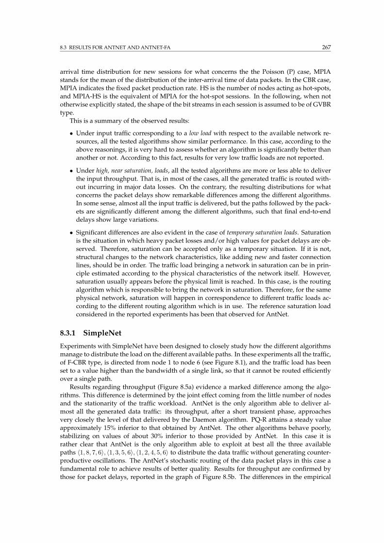
8.3 RESULTS FOR ANTNET AND ANTNET-FA 267
arrival time distribution for new sessions for what concerns the the Poisson (P) case, MPIA
stands for the mean of the distribution of the inter-arrival time of data packets. In the CBR case,
MPIA indicates the fixed packet production rate. HS is the number of nodes acting as hot-spots,
and MPIA-HS is the equivalent of MPIA for the hot-spot sessions. In the following, when not
otherwise explicitly stated, the shape of the bit streams in each session is assumed to be of GVBR
type.
This is a summary of the observed results:
• Under input traffic corresponding to a low load with respect to the available network re-
sources, all the tested algorithms show similar performance. In this case, according to the
above reasonings, it is very hard to assess whether an algorithm is significantly better than
another or not. According to this fact, results for very low traffic loads are not reported.
• Under high, near saturation, loads, all the tested algorithms are more or less able to deliver
the input throughput. That is, in most of the cases, all the generated traffic is routed with-
out incurring in major data losses. On the contrary, the resulting distributions for what
concerns the packet delays show remarkable differences among the different algorithms.
In some sense, almost all the input traffic is delivered, but the paths followed by the pack-
ets are significantly different among the different algorithms, such that final end-to-end
delays show large variations.
• Significant differences are also evident in the case of temporary saturation loads. Saturation
is the situation in which heavy packet losses and/or high values for packet delays are ob-
served. Therefore, saturation can be accepted only as a temporary situation. If it is not,
structural changes to the network characteristics, like adding new and faster connection
lines, should be in order. The traffic load bringing a network in saturation can be in prin-
ciple estimated according to the physical characteristics of the network itself. However,
saturation usually appears before the physical limit is reached. In this case, is the routing
algorithm which is responsible to bring the network in saturation. Therefore, for the same
physical network, saturation will happen in correspondence to different traffic loads ac-
cording to the different routing algorithm which is in use. The reference saturation load
considered in the reported experiments has been that observed for AntNet.
8.3.1 SimpleNet
Experiments with SimpleNet have been designed to closely study how the different algorithms
manage to distribute the load on the different available paths. In these experiments all the traffic,
of F-CBR type, is directed from node 1 to node 6 (see Figure 8.1), and the traffic load has been
set to a value higher than the bandwidth of a single link, so that it cannot be routed efficiently
over a single path.
Results regarding throughput (Figure 8.5a) evidence a marked difference among the algo-
rithms. This difference is determined by the joint effect coming from the little number of nodes
and the stationarity of the traffic workload. AntNet is the only algorithm able to deliver al-
most all the generated data traffic: its throughput, after a short transient phase, approaches
very closely the level of that delivered by the Daemon algorithm. PQ-R attains a steady value
approximately 15% inferior to that obtained by AntNet. The other algorithms behave poorly,
stabilizing on values of about 30% inferior to those provided by AntNet. In this case it is
rather clear that AntNet is the only algorithm able to exploit at best all the three available
paths 〈1, 8, 7, 6〉, 〈1, 3, 5, 6〉, 〈1, 2, 4, 5, 6〉 to distribute the data traffic without generating counter-
productive oscillations. The AntNet’s stochastic routing of the data packet plays in this case a
fundamental role to achieve results of better quality. Results for throughput are confirmed by
those for packet delays, reported in the graph of Figure 8.5b. The differences in the empirical
268 8. EXPERIMENTAL RESULTS FOR ACO ROUTING ALGORITHMS
distributions for packet delays reflect approximatively the same proportions evidenced in the
throughput case.
9.5
10.0
10.5
11.0
11.5
12.0
12.5
13.0
13.5
14.0
0 100 200 300 400 500 600 700 800 900 1000
Thr
ough
put (
106 b
it/se
c)
Simulation Time (sec)
OSPFSPF
BFQ-R
PQ-RAntNet
Daemon
(a)
0.0
0.2
0.4
0.6
0.8
1.0
0 0.05 0.1 0.15 0.2
Em
piric
al D
istr
ibut
ion
Packet Delay (sec)
OSPFSPF
BFQ-R
PQ-RAntNet
Daemon
(b)
Figure 8.5: SimpleNet: Comparison of algorithms for F-CBR traffic directed from node 1 to node 6 (MPIA = 0.0003sec). (a) Throughput, and (b) empirical distribution of the end-to-end data packet delays.
8.3.2 NSFNET
Performance on NSFNET have been tested using UP, RP, UP-HS and TMPHS-UP traffic patterns.
For all the considered cases, all the algorithms behave similarly with respect to throughput,
while major differences are apparent for packet delays. For each one of the UP, RP and UP-
HS cases, we have ran a sequence of five distinct experiments sets, each of ten repeated trials.
The generated workload is gradually increased at each set starting from an initial low workload
until a near-saturation one is reached. The workload is increased by reducing the time interval
between sessions’ inter-arrivals.
UP TRAFFIC - WORKLOAD RANGING FROM LOW TO NEAR-SATURATION
In this case, differences in throughput (Figure 8.6a) are small: the best performing algorithms are
BF and SPF, which can attain performance of only about 10% inferior to those of Daemon, and
of the same amount better than those of AntNet, Q-R and PQ-R,3 while OSPF behaves slightly
better than these last ones. Concerning delays (Figure 8.6b) the picture is rather different: it
seems that all the algorithms but AntNet have been able to produce a quite good throughput at
the expenses of a much worse result for end-to-end delays, as it will also happen in the majority
of the ran experiments. OSPF, Q-R and PQ-R show really poor results (delays of order 2 or more
seconds have to be considered as very high values, even if considering the 90-th percentile of the
distribution). BF and SPF show a similar behavior, with performance of order 50% worse than
those obtained by AntNet and of order 65% worse than Daemon.
3 In these and in some of the experiments presented in the following, PQ-R’s performance is slightly worse than thatof Q-R. This seems to be in contrast with the results presented by the PQ-R’s authors in the article where they introducedPQ-R [84]. A possible explanation of such a behavior the fact that: (i) their link recovery rate has been designed havingin mind a discrete-time system while in the ran simulations time is a continuous variable, and (ii) the experimentaland simulation conditions are rather different, due to the fact that the simulator they have used is quite far from beingrealistic. Moreover, in the paper the way traffic patterns are generated is not specified.

8.3 RESULTS FOR ANTNET AND ANTNET-FA 269
0
2
4
6
8
10
14
16
18
AntNet OSPF SPF BF Q-R PQ-R Daemon
Thro
ughput (1
06
bit/
sec)
2.4 2.3 2.2 2.1 2
1→ 2
(a)
0.0
0.5
1.0
1.5
2.0
2.5
3.0
3.5
4.0
4.5
AntNet OSPF SPF BF Q-R PQ-R Daemon90-t
h p
erc
entil
e o
f pack
et dela
ys (
sec)
2.4 2.3 2.2 2.1 2
(b)
Figure 8.6: NSFNET: Comparison of algorithms for increasing workload under UP traffic conditions. The load isincreased by reducing the MSIA value from 2.4 to 2 seconds (MPIA = 0.005 sec). (a) Throughput, and (b) 90-thpercentile of the empirical distribution of the end-to-end data packet delays.
RP TRAFFIC - WORKLOAD RANGING FROM LOW TO NEAR-SATURATION
In the RP case (Figure 8.7a), the throughput generated by AntNet, SPF and BF look very similar,
although AntNet shows a slightly better performance. OSPF and PQ-R behave only slightly
worse than SPF and BF, while Q-R is the worst performing algorithm. Daemon is able to obtain
only slightly better results than AntNet. Again, looking at the results for end-to-end delays
(Figure 8.7b), OSPF, Q-R and PQ-R perform quite bad, while SPF’s results are a bit better than
those of BF but of order 40%worse than those of AntNet. Daemon is in this case far better, which
might be an indication of the fact that the testbed was rather difficult.
0
2
4
6
8
10
AntNet OSPF SPF BF Q-R PQ-R Daemon
Thro
ughput (1
06
bit/
sec)
2.8 2.7 2.6 2.5 2.41→ 2
(a)
0.0
0.5
1.0
1.5
2.0
2.5
3.0
3.5
4.0
AntNet OSPF SPF BF Q-R PQ-R Daemon90-t
h p
erc
entil
e o
f pack
et dela
ys (
sec)
2.8 2.7 2.6 2.5 2.4
(b)
Figure 8.7: NSFNET: Comparison of algorithms for increasing workload under RP traffic conditions. The load isincreased by reducing the MSIA value from 2.8 to 2.4 seconds (MPIA = 0.005 sec). (a) Throughput, and (b) 90-thpercentile of the empirical distribution of the end-to-end data packet delays.
UP-HS TRAFFIC - WORKLOAD RANGING FROM LOW TO NEAR-SATURATION
In this case packet burstiness is set to a much lower level than in the previous cases due to
the additional load given by the hot spots. Throughput (Figure 8.8a) for AntNet, SPF, BF, Q-R
and Daemon are very similar, while OSPF and PQ-R clearly obtain much worse results. Again
(Figure 8.8b), end-to-end delays results for OSPF, Q-R and PQ-R are much worse than those for
the other algorithms (they are so much worse that actually they do not fit in the chosen scale).
270 8. EXPERIMENTAL RESULTS FOR ACO ROUTING ALGORITHMS
AntNet is still the best performing algorithm. In this case, differences with SPF are of order 20%,
and of 40%with respect to BF. Daemon performs about 50% better than AntNet and scales much
better than AntNet, which, again, indicates that the testbed was rather difficult.
0
2
4
6
8
10
14
16
18
AntNet OSPF SPF BF Q-R PQ-R Daemon
Thro
ughput (1
06
bit/
sec)
2.4 2.3 2.2 2.1 2
1→ 2
(a)
0.0
0.1
0.2
0.3
0.4
0.5
AntNet OSPF SPF BF Q-R PQ-R Daemon90-t
h p
erc
entil
e o
f pack
et dela
ys (
sec)
2.4 2.3 2.2 2.1 2
(b)
Figure 8.8: NSFNET: Comparison of algorithms for increasing load for UP-HS traffic. The load is increased byreducing the MSIA value from 2.4 to 2.0 seconds (MPIA = 0.3 sec, HS = 4, MPIA-HS = 0.04 sec). (a) Throughput,and (b) 90-th percentile of the empirical distribution of the end-to-end data packet delays.
TMPHS-UP TRAFFIC
Figure 8.9 shows how the algorithms behave in the case of a TMPHS-UP situation. At time t =
400 four hot spot nodes are turned on and superimposed to the existing, light, UP traffic (packet
burstiness for the HS sessions is much higher than that for the UP sessions). The transient is held
for 120 seconds. The graph shows the details of the typical answer curves observed during the
experiments. Reported values are a sort of “instantaneous” values for throughput and packet
delays, computed as the average of the values observed during moving time windows of 5
seconds. Most of the algorithms have a similar, very good, performance as far as throughput is
concerned. Only OSPF and PQ-R, lose a few percent of the packets during the transitory period.
The graph of packet delays confirms previous results. SPF and BF show similar behavior, with
performance of about 20% worse than AntNet and 45% worse than Daemon. The other three
algorithms show a big out-of-scale jump, clearly being unable to adapt properly to the sudden
increase in the workload.
8.3.3 NTTnet
The same set of experiments run on NSFNET have been also run on NTTnet. Results are in
this case even sharper than those obtained with NSFNET: AntNet clearly outperforms all the
competitor algorithms.
UP TRAFFIC - WORKLOAD RANGING FROM LOW TO NEAR-SATURATION
In the UP case, as well as, in the RP and UP-HS cases, differences in throughput are not signifi-
cant (Figures 8.10a, 8.11a and 8.12a). All the algorithms, with the exception of OSPF, are able to
deliver more or less the same throughput as Daemon does.
Concerning delays (Figure 8.10b), differences between AntNet and the other algorithms are
of one or more orders of magnitude. AntNet’s packet delays are very close to those obtained by
Daemon. SPF is the third best, but its performance is about of 80% worse than that of AntNet.
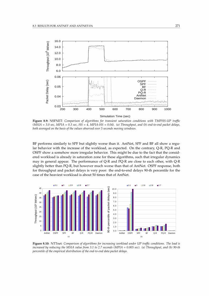
8.3 RESULTS FOR ANTNET AND ANTNET-FA 271
6.0
8.0
10.0
12.0
14.0
16.0
Thro
ughp
ut (1
06 bit/
sec)
OSPFSPF
BFQ-R
PQ-RAntNet
Daemon
0.03
0.04
0.05
0.06
200 300 400 500 600 700 800 900 1000
Pac
ket D
elay
(sec
)
Simulation Time (sec)
Figure 8.9: NSFNET: Comparison of algorithms for transient saturation conditions with TMPHS-UP traffic(MSIA = 3.0 sec, MPIA = 0.3 sec, HS = 4, MPIA-HS = 0.04). (a) Throughput, and (b) end-to-end packet delays,both averaged on the basis of the values observed over 5 seconds moving windows.
BF performs similarly to SPF but slightly worse than it. AntNet, SPF and BF all show a regu-
lar behavior with the increase of the workload, as expected. On the contrary, Q-R, PQ-R and
OSPF show a somehow more irregular behavior. This might be due to the fact that the consid-
ered workload is already in saturation zone for these algorithms, such that irregular dynamics
may in general appear. The performance of Q-R and PQ-R are close to each other, with Q-R
slightly better than PQ-R, but however much worse than that of AntNet. OSPF response, both
for throughput and packet delays is very poor: the end-to-end delays 90-th percentile for the
case of the heaviest workload is about 50 times that of AntNet.
0
5
10
15
20
25
30
35
40
45
AntNet OSPF SPF BF Q-R PQ-R Daemon
Thro
ughput (1
06
bit/
sec)
3.1 3 2.9 2.8 2.7
(a)
0.0
1.0
2.0
3.0
4.0
5.0
6.0
7.0
8.0
9.0
10.0
AntNet OSPF SPF BF Q-R PQ-R Daemon90-t
h p
erc
entil
e o
f pack
et dela
ys (
sec)
3.1 3 2.9 2.8 2.7
(b)
Figure 8.10: NTTnet: Comparison of algorithms for increasing workload under UP traffic conditions. The load isincreased by reducing the MSIA value from 3.1 to 2.7 seconds (MPIA = 0.005 sec). (a) Throughput, and (b) 90-thpercentile of the empirical distribution of the end-to-end data packet delays.
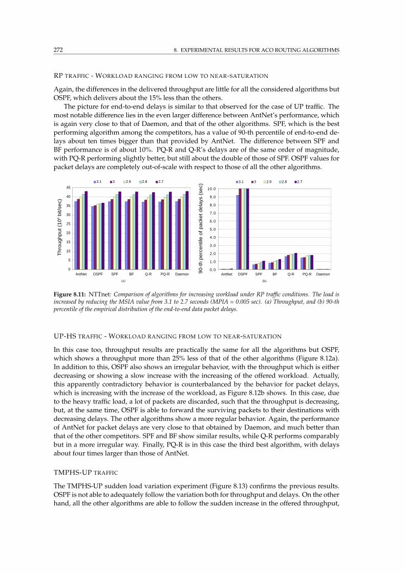
272 8. EXPERIMENTAL RESULTS FOR ACO ROUTING ALGORITHMS
RP TRAFFIC - WORKLOAD RANGING FROM LOW TO NEAR-SATURATION
Again, the differences in the delivered throughput are little for all the considered algorithms but
OSPF, which delivers about the 15% less than the others.
The picture for end-to-end delays is similar to that observed for the case of UP traffic. The
most notable difference lies in the even larger difference between AntNet’s performance, which
is again very close to that of Daemon, and that of the other algorithms. SPF, which is the best
performing algorithm among the competitors, has a value of 90-th percentile of end-to-end de-
lays about ten times bigger than that provided by AntNet. The difference between SPF and
BF performance is of about 10%. PQ-R and Q-R’s delays are of the same order of magnitude,
with PQ-R performing slightly better, but still about the double of those of SPF. OSPF values for
packet delays are completely out-of-scale with respect to those of all the other algorithms.
0
5
10
15
20
25
30
35
40
45
AntNet OSPF SPF BF Q-R PQ-R Daemon
Thro
ughput (1
06
bit/
sec)
3.1 3 2.9 2.8 2.7
(a)
0.0
1.0
2.0
3.0
4.0
5.0
6.0
7.0
8.0
9.0
10.0
AntNet OSPF SPF BF Q-R PQ-R Daemon90-t
h p
erc
entil
e o
f pack
et dela
ys (
sec)
3.1 3 2.9 2.8 2.7
(b)
Figure 8.11: NTTnet: Comparison of algorithms for increasing workload under RP traffic conditions. The load isincreased by reducing the MSIA value from 3.1 to 2.7 seconds (MPIA = 0.005 sec). (a) Throughput, and (b) 90-thpercentile of the empirical distribution of the end-to-end data packet delays.
UP-HS TRAFFIC - WORKLOAD RANGING FROM LOW TO NEAR-SATURATION
In this case too, throughput results are practically the same for all the algorithms but OSPF,
which shows a throughput more than 25% less of that of the other algorithms (Figure 8.12a).
In addition to this, OSPF also shows an irregular behavior, with the throughput which is either
decreasing or showing a slow increase with the increasing of the offered workload. Actually,
this apparently contradictory behavior is counterbalanced by the behavior for packet delays,
which is increasing with the increase of the workload, as Figure 8.12b shows. In this case, due
to the heavy traffic load, a lot of packets are discarded, such that the throughput is decreasing,
but, at the same time, OSPF is able to forward the surviving packets to their destinations with
decreasing delays. The other algorithms show a more regular behavior. Again, the performance
of AntNet for packet delays are very close to that obtained by Daemon, and much better than
that of the other competitors. SPF and BF show similar results, while Q-R performs comparably
but in a more irregular way. Finally, PQ-R is in this case the third best algorithm, with delays
about four times larger than those of AntNet.
TMPHS-UP TRAFFIC
The TMPHS-UP sudden load variation experiment (Figure 8.13) confirms the previous results.
OSPF is not able to adequately follow the variation both for throughput and delays. On the other
hand, all the other algorithms are able to follow the sudden increase in the offered throughput,
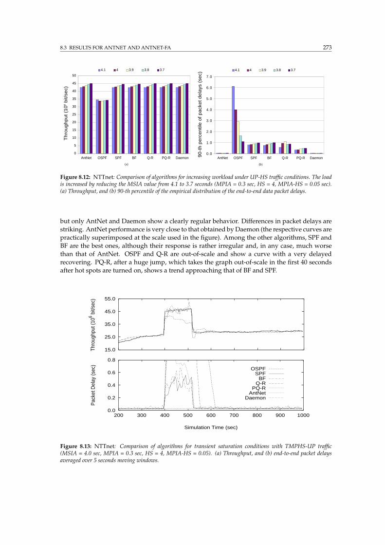
8.3 RESULTS FOR ANTNET AND ANTNET-FA 273
0
5
10
15
20
25
30
35
40
45
50
AntNet OSPF SPF BF Q-R PQ-R Daemon
Thro
ughput (1
06
bit/
sec)
4.1 4 3.9 3.8 3.7
(a)
0.0
1.0
2.0
3.0
4.0
5.0
6.0
7.0
AntNet OSPF SPF BF Q-R PQ-R Daemon90-t
h p
erc
entil
e o
f pack
et dela
ys (
sec)
4.1 4 3.9 3.8 3.7
(b)
Figure 8.12: NTTnet: Comparison of algorithms for increasing workload under UP-HS traffic conditions. The loadis increased by reducing the MSIA value from 4.1 to 3.7 seconds (MPIA = 0.3 sec, HS = 4, MPIA-HS = 0.05 sec).(a) Throughput, and (b) 90-th percentile of the empirical distribution of the end-to-end data packet delays.
but only AntNet and Daemon show a clearly regular behavior. Differences in packet delays are
striking. AntNet performance is very close to that obtained byDaemon (the respective curves are
practically superimposed at the scale used in the figure). Among the other algorithms, SPF and
BF are the best ones, although their response is rather irregular and, in any case, much worse
than that of AntNet. OSPF and Q-R are out-of-scale and show a curve with a very delayed
recovering. PQ-R, after a huge jump, which takes the graph out-of-scale in the first 40 seconds
after hot spots are turned on, shows a trend approaching that of BF and SPF.
15.0
25.0
35.0
45.0
55.0
Thro
ughp
ut (1
06 bit/
sec)
OSPFSPF
BFQ-R
PQ-RAntNet
Daemon
0.0
0.2
0.4
0.6
0.8
200 300 400 500 600 700 800 900 1000
Pac
ket D
elay
(sec
)
Simulation Time (sec)
Figure 8.13: NTTnet: Comparison of algorithms for transient saturation conditions with TMPHS-UP traffic(MSIA = 4.0 sec, MPIA = 0.3 sec, HS = 4, MPIA-HS = 0.05). (a) Throughput, and (b) end-to-end packet delaysaveraged over 5 seconds moving windows.
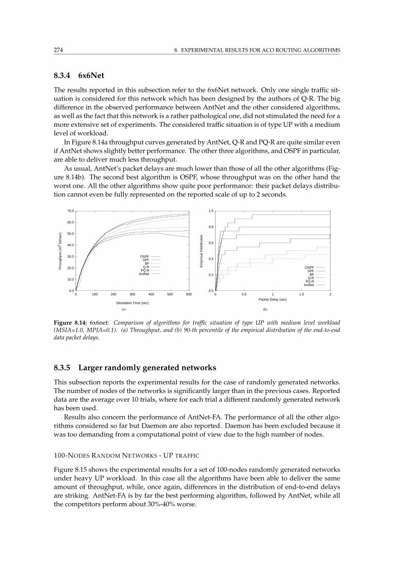
274 8. EXPERIMENTAL RESULTS FOR ACO ROUTING ALGORITHMS
8.3.4 6x6Net
The results reported in this subsection refer to the 6x6Net network. Only one single traffic sit-
uation is considered for this network which has been designed by the authors of Q-R. The big
difference in the observed performance between AntNet and the other considered algorithms,
as well as the fact that this network is a rather pathological one, did not stimulated the need for a
more extensive set of experiments. The considered traffic situation is of type UP with a medium
level of workload.
In Figure 8.14a throughput curves generated by AntNet, Q-R and PQ-R are quite similar even
if AntNet shows slightly better performance. The other three algorithms, and OSPF in particular,
are able to deliver much less throughput.
As usual, AntNet’s packet delays are much lower than those of all the other algorithms (Fig-
ure 8.14b). The second best algorithm is OSPF, whose throughput was on the other hand the
worst one. All the other algorithms show quite poor performance: their packet delays distribu-
tion cannot even be fully represented on the reported scale of up to 2 seconds.
0.0
10.0
20.0
30.0
40.0
50.0
60.0
70.0
0 100 200 300 400 500 600
Thr
ough
put (
106 b
it/se
c)
Simulation Time (sec)
OSPFSPF
BFQ-R
PQ-RAntNet
(a)
0.0
0.2
0.4
0.6
0.8
1.0
0 0.5 1 1.5 2
Em
piric
al D
istr
ibut
ion
Packet Delay (sec)
OSPFSPF
BFQ-R
PQ-RAntNet
(b)
Figure 8.14: 6x6net: Comparison of algorithms for traffic situation of type UP with medium level workload(MSIA=1.0, MPIA=0.1). (a) Throughput, and (b) 90-th percentile of the empirical distribution of the end-to-enddata packet delays.
8.3.5 Larger randomly generated networks
This subsection reports the experimental results for the case of randomly generated networks.
The number of nodes of the networks is significantly larger than in the previous cases. Reported
data are the average over 10 trials, where for each trial a different randomly generated network
has been used.
Results also concern the performance of AntNet-FA. The performance of all the other algo-
rithms considered so far but Daemon are also reported. Daemon has been excluded because it
was too demanding from a computational point of view due to the high number of nodes.
100-NODES RANDOM NETWORKS - UP TRAFFIC
Figure 8.15 shows the experimental results for a set of 100-nodes randomly generated networks
under heavy UP workload. In this case all the algorithms have been able to deliver the same
amount of throughput, while, once again, differences in the distribution of end-to-end delays
are striking. AntNet-FA is by far the best performing algorithm, followed by AntNet, while all
the competitors perform about 30%-40% worse.
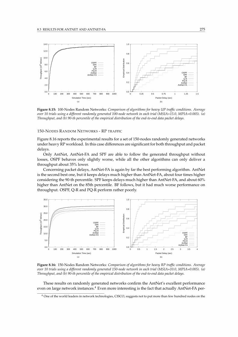
8.3 RESULTS FOR ANTNET AND ANTNET-FA 275
0.0
2.0
4.0
6.0
8.0
10.0
12.0
14.0
0 100 200 300 400 500 600 700 800 900 1000
Thr
ough
put (
106 b
it/se
c)
Simulation Time (sec)
OSPFSPF
BFQ-R
PQ-RAntNet
AntNet-FA
(a)
0.0
0.2
0.4
0.6
0.8
1.0
0 0.25 0.5 0.75 1 1.25 1.5
Em
piric
al D
istr
ibut
ion
Packet Delay (sec)
OSPFSPF
BFQ-R
PQ-RAntNet
AntNet-FA
(b)
Figure 8.15: 100-Nodes Random Networks: Comparison of algorithms for heavy UP traffic conditions. Averageover 10 trials using a different randomly generated 100-node network in each trial (MSIA=15.0, MPIA=0.005). (a)Throughput, and (b) 90-th percentile of the empirical distribution of the end-to-end data packet delays.
150-NODES RANDOM NETWORKS - RP TRAFFIC
Figure 8.16 reports the experimental results for a set of 150-nodes randomly generated networks
under heavy RPworkload. In this case differences are significant for both throughput and packet
delays.
Only AntNet, AntNet-FA and SPF are able to follow the generated throughput without
losses, OSPF behaves only slightly worse, while all the other algorithms can only deliver a
throughput about 35% lower.
Concerning packet delays, AntNet-FA is again by far the best performing algorithm. AntNet
is the second best one, but it keeps delays much higher than AntNet-FA, about four times higher
considering the 90-th percentile. SPF keeps delays much higher than AntNet-FA, and about 60%
higher than AntNet on the 85th percentile. BF follows, but it had much worse performance on
throughput. OSPF, Q-R and PQ-R perform rather poorly.
0.0
5.0
10.0
15.0
20.0
25.0
30.0
35.0
0 100 200 300 400 500 600 700 800 900 1000
Thr
ough
put (
106 b
it/se
c)
Simulation Time (sec)
OSPFSPF
BFQ-R
PQ-RAntNet
AntNet-FA
(a)
0.0
0.2
0.4
0.6
0.8
1.0
0 0.5 1 1.5 2 2.5 3 3.5 4
Em
piric
al D
istr
ibut
ion
Packet Delay (sec)
OSPFSPF
BFQ-R
PQ-RAntNet
AntNet-FA
(b)
Figure 8.16: 150-Nodes Random Networks: Comparison of algorithms for heavy RP traffic conditions. Averageover 10 trials using a different randomly generated 150-node network in each trial (MSIA=10.0, MPIA=0.005). (a)Throughput, and (b) 90-th percentile of the empirical distribution of the end-to-end data packet delays.
These results on randomly generated networks confirm the AntNet’s excellent performance
even on large network instances.4 Even more interesting is the fact that actually AntNet-FA per-
4 One of the world leaders in network technologies, CISCO, suggests not to put more than few hundred nodes on the
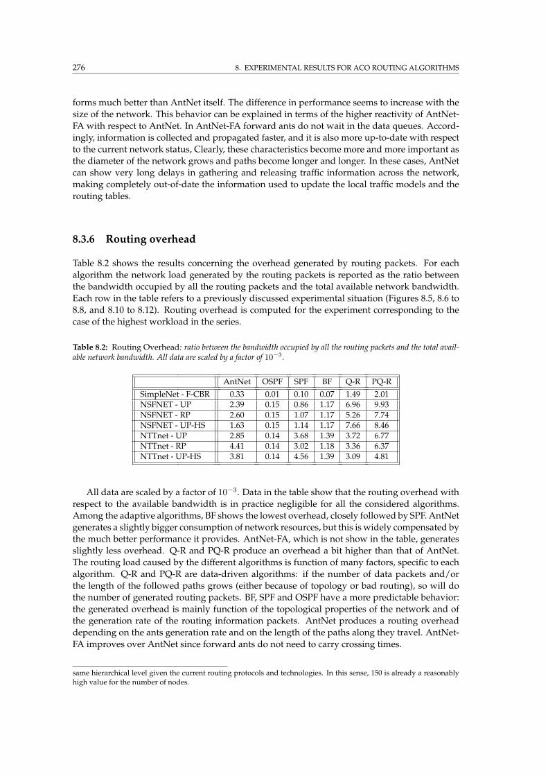
276 8. EXPERIMENTAL RESULTS FOR ACO ROUTING ALGORITHMS
forms much better than AntNet itself. The difference in performance seems to increase with the
size of the network. This behavior can be explained in terms of the higher reactivity of AntNet-
FA with respect to AntNet. In AntNet-FA forward ants do not wait in the data queues. Accord-
ingly, information is collected and propagated faster, and it is also more up-to-date with respect
to the current network status, Clearly, these characteristics become more and more important as
the diameter of the network grows and paths become longer and longer. In these cases, AntNet
can show very long delays in gathering and releasing traffic information across the network,
making completely out-of-date the information used to update the local traffic models and the
routing tables.
8.3.6 Routing overhead
Table 8.2 shows the results concerning the overhead generated by routing packets. For each
algorithm the network load generated by the routing packets is reported as the ratio between
the bandwidth occupied by all the routing packets and the total available network bandwidth.
Each row in the table refers to a previously discussed experimental situation (Figures 8.5, 8.6 to
8.8, and 8.10 to 8.12). Routing overhead is computed for the experiment corresponding to the
case of the highest workload in the series.
Table 8.2: Routing Overhead: ratio between the bandwidth occupied by all the routing packets and the total avail-able network bandwidth. All data are scaled by a factor of 10−3.
AntNet OSPF SPF BF Q-R PQ-R
SimpleNet - F-CBR 0.33 0.01 0.10 0.07 1.49 2.01NSFNET - UP 2.39 0.15 0.86 1.17 6.96 9.93NSFNET - RP 2.60 0.15 1.07 1.17 5.26 7.74NSFNET - UP-HS 1.63 0.15 1.14 1.17 7.66 8.46NTTnet - UP 2.85 0.14 3.68 1.39 3.72 6.77NTTnet - RP 4.41 0.14 3.02 1.18 3.36 6.37NTTnet - UP-HS 3.81 0.14 4.56 1.39 3.09 4.81
All data are scaled by a factor of 10−3. Data in the table show that the routing overhead with
respect to the available bandwidth is in practice negligible for all the considered algorithms.
Among the adaptive algorithms, BF shows the lowest overhead, closely followed by SPF. AntNet
generates a slightly bigger consumption of network resources, but this is widely compensated by
the much better performance it provides. AntNet-FA, which is not show in the table, generates
slightly less overhead. Q-R and PQ-R produce an overhead a bit higher than that of AntNet.
The routing load caused by the different algorithms is function of many factors, specific to each
algorithm. Q-R and PQ-R are data-driven algorithms: if the number of data packets and/or
the length of the followed paths grows (either because of topology or bad routing), so will do
the number of generated routing packets. BF, SPF and OSPF have a more predictable behavior:
the generated overhead is mainly function of the topological properties of the network and of
the generation rate of the routing information packets. AntNet produces a routing overhead
depending on the ants generation rate and on the length of the paths along they travel. AntNet-
FA improves over AntNet since forward ants do not need to carry crossing times.
same hierarchical level given the current routing protocols and technologies. In this sense, 150 is already a reasonablyhigh value for the number of nodes.
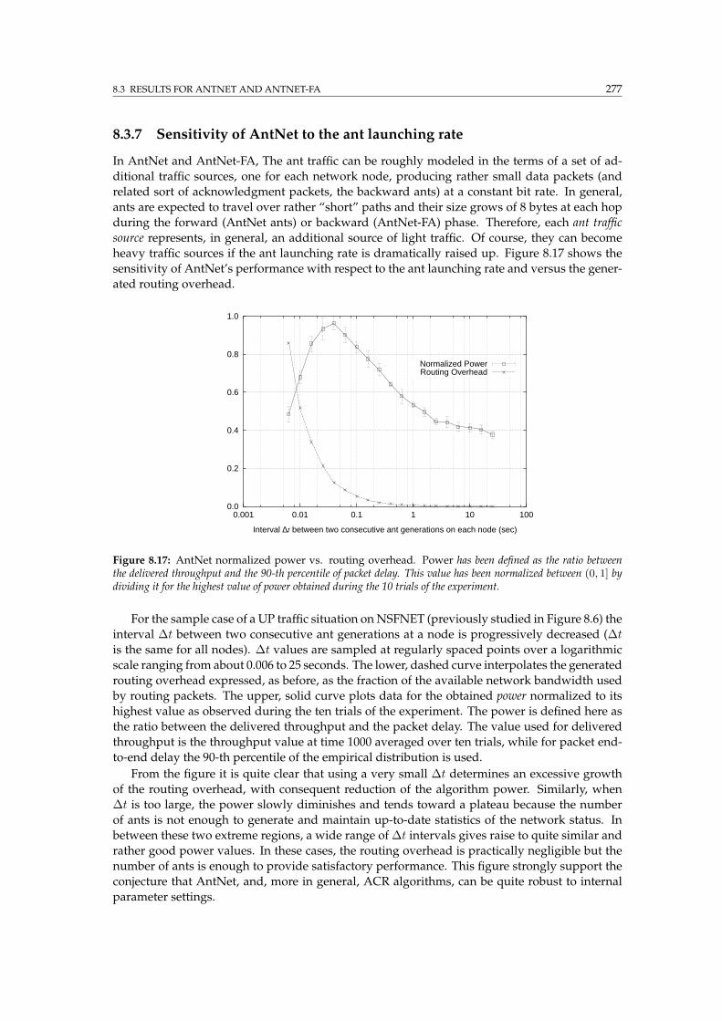
8.3 RESULTS FOR ANTNET AND ANTNET-FA 277
8.3.7 Sensitivity of AntNet to the ant launching rate
In AntNet and AntNet-FA, The ant traffic can be roughly modeled in the terms of a set of ad-
ditional traffic sources, one for each network node, producing rather small data packets (and
related sort of acknowledgment packets, the backward ants) at a constant bit rate. In general,
ants are expected to travel over rather “short” paths and their size grows of 8 bytes at each hop
during the forward (AntNet ants) or backward (AntNet-FA) phase. Therefore, each ant traffic
source represents, in general, an additional source of light traffic. Of course, they can become
heavy traffic sources if the ant launching rate is dramatically raised up. Figure 8.17 shows the
sensitivity of AntNet’s performance with respect to the ant launching rate and versus the gener-
ated routing overhead.
0.0
0.2
0.4
0.6
0.8
1.0
0.001 0.01 0.1 1 10 100
Interval ∆t between two consecutive ant generations on each node (sec)
Normalized PowerRouting Overhead
Figure 8.17: AntNet normalized power vs. routing overhead. Power has been defined as the ratio betweenthe delivered throughput and the 90-th percentile of packet delay. This value has been normalized between (0, 1] bydividing it for the highest value of power obtained during the 10 trials of the experiment.
For the sample case of a UP traffic situation onNSFNET (previously studied in Figure 8.6) the
interval ∆t between two consecutive ant generations at a node is progressively decreased (∆t
is the same for all nodes). ∆t values are sampled at regularly spaced points over a logarithmic
scale ranging from about 0.006 to 25 seconds. The lower, dashed curve interpolates the generated
routing overhead expressed, as before, as the fraction of the available network bandwidth used
by routing packets. The upper, solid curve plots data for the obtained power normalized to its
highest value as observed during the ten trials of the experiment. The power is defined here as
the ratio between the delivered throughput and the packet delay. The value used for delivered
throughput is the throughput value at time 1000 averaged over ten trials, while for packet end-
to-end delay the 90-th percentile of the empirical distribution is used.
From the figure it is quite clear that using a very small ∆t determines an excessive growth
of the routing overhead, with consequent reduction of the algorithm power. Similarly, when
∆t is too large, the power slowly diminishes and tends toward a plateau because the number
of ants is not enough to generate and maintain up-to-date statistics of the network status. In
between these two extreme regions, a wide range of ∆t intervals gives raise to quite similar and
rather good power values. In these cases, the routing overhead is practically negligible but the
number of ants is enough to provide satisfactory performance. This figure strongly support the
conjecture that AntNet, and, more in general, ACR algorithms, can be quite robust to internal
parameter settings.

278 8. EXPERIMENTAL RESULTS FOR ACO ROUTING ALGORITHMS
8.3.8 Efficacy of adaptive path evaluation in AntNet
At a first glance, the mechanisms used by AntNet and AntNet-FA to assign reinforcement values
might seem over-complicate. Subsection 7.1.4 has discussed in depth the need for such mecha-
nisms, and, accordingly, the need to maintain at each node a local model for the network-wide
traffic patterns.
In Figure 8.18 we report the outcome of a simple experiment that compare the performance
of AntNet without path evaluation (i.e., making use of an assigned constant value for the rein-
forcements whatever path is followed), with the performance of the usual AntNet, making use
of path evaluation and therefore of possibly non-constant reinforcements.
4e+06
6e+06
8e+06
1e+07
1.2e+07
1.4e+07
1.6e+07
1.8e+07
2e+07
0.001 0.01 0.1 1 10 100
Thr
ough
put /
90-
th D
elay
Per
cent
ile (
106 b
it/se
c2 )
Interval ∆t between two consecutive ant generations on each node (sec)
AntNet with r ≠ Const.AntNet with r = Const.
Figure 8.18: Constant vs. non-constant reinforcements: AntNet power for increasing values of ant generationrates at each node. The results are averages over 10 trials for UP traffic conditions on NSFNET.
In the case of the use of constant reinforcements, what is at work in AntNet is the implicit re-
inforcement mechanism due to the differentiation in the ant arrival rates explained at Page 217.
Ants traveling along faster paths will arrive at a higher rate than other ants, hence their paths
will receive a higher cumulative reward. In AntNet-FA this effect is much reduced. The fig-
ure shows that, in spite of its simplicity, the implicit reinforcement mechanism is already quite
effective but, in the range of the ant generation rates corresponding to the higher power val-
ues, the difference between the two algorithms can reach about 30%. Such a difference surely
justifies the additional complexity associated to path evaluation and to the use of non-constant
reinforcements.
8.4 Experimental settings and results for AntHocNet
We report in this section some preliminary experimental results for AntHocNet. As simulation
software we have used Qualnet [354], a discrete-event packet-level simulator developed by Scal-
able Networks Inc. as a follow-up of GloMoSim, which was a shareware simulator designed at
University of California, Los Angeles. Qualnet is specifically optimized to simulate large-scale
MANETs, and comes with correct implementations of the most important protocols for all the
network layers and for routing in particular. We have compared the performance of AntHocNet
with Ad Hoc On-Demand Distance Vector (AODV) [349] (with local route repair and expanding
ring search, e.g., [268]), a state-of-the-art MANET routing algorithm and a de facto standard.
AODV is a purely reactive approach. Single-path routes are established on-demand and on the
8.4 EXPERIMENTAL SETTINGS AND RESULTS FOR ANTHOCNET 279
basis on aminimum-hopmetric. Only the nodes along the path used by the applicationmaintain
routing information toward the destination, such that in practice a virtual-circuit is established
and end-to-end signaling is used tear up and down the path, as well as to rebuild the path in
case of broken links.
Most of our simulation scenarios, except for the scalability study scenario which is taken
from [268], are derived from the base scenario used in [61], which is so far a constant reference
in the current MANET literature, even if it is quite pathological and not really general. In this
base scenario 50 nodes are randomly placed in a rectangular area of 1500 × 300 m2. Within
this area, the nodes move according to the random waypoint model [236]: each node randomly
chooses a destination point and a speed, and moves to this point with the chosen speed. After
that it stops for a certain pause time and then randomly chooses a new destination and speed.
The maximum speed in the scenario is 20 meters/sec and the pause time is 30 seconds. The total
length of the simulation is 900 seconds. Data traffic is generated by 20 constant bit rate (CBR)
sources sending one 64-byte packet per second. Each source starts sending at a random time
between 0 and 180 seconds after the start of the simulation, and keeps sending until the end. At
the physical layer we use a two-ray signal propagation model. The transmission range is around
300 meters, and the data rate is 2 Mbit/sec. At the MAC layer we use the popular 802.11 DCF
protocol.
In this scenario nodes are densely packed, such that from one side there is a high probability
of radio collisions but from the other side it is always possible to easily find a short route to a
destination. The average path length is about two hops and the average number of neighbors
of a node is about ten (due to the dimensions of the node area vs. the radio range and the fact
that random waypoint movements tend to concentrate nodes in the central zone of the area).
This is clearly a scenario that well match the characteristics of a purely reactive algorithm like
AODV since it is relatively easy and fast to build or re-build a path while at the same time
is important to keep low the routing overhead in order to reduce the risk of radio collisions.
Moreover, since it is quite hard to find multiple (and good) radio-disjoint paths for the same
destination given the high node density, the AODV’s single-path strategy minimizing the hop
number appears as the most suitable one. On the other hand, AntHocNet is a hybrid, reactive-
proactive, algorithm for multi-path routing using both end-to-end delay and hop metrics to
define the paths. In order to study the behavior of the two algorithms under this reference
scenario but also under possibly more interesting and challenging conditions involving longer
path lengths and less dense networks, we have performed extensive simulations changing the
pause time, the node area and the number of nodes. For each new scenario, 5 different problems
have been created, by choosing different initial placements of the nodes and different movement
patterns. The reported results, in terms of delivery ratio (fraction of sent packets which actually
arrives at their destination) and end-to-end delay, are averaged over 5 different runs (to account
for stochastic elements, both in the algorithms and in the physical and MAC layers) on each of
the 5 problems.
Since AntHocNet generate considerably more routing packets than AODV, we have also
made a further study increasing the number of nodes up to 2000 in order to study the over-
all scalability of the approach.
Increasing number of hops and node sparseness
We have progressively extended the long side of the simulation area. This has a double effect:
paths become longer and the network becomes sparser. The results are shown in Figure 8.19. In
the base scenario, AntHocNet has a better delivery ratio than AODV, but a higher average delay.
For the longer areas, the difference in delivery ratio becomes bigger, and AODV also looses its
advantage in delay. If we take a look at the 99-th percentile of the delay, we can see that the
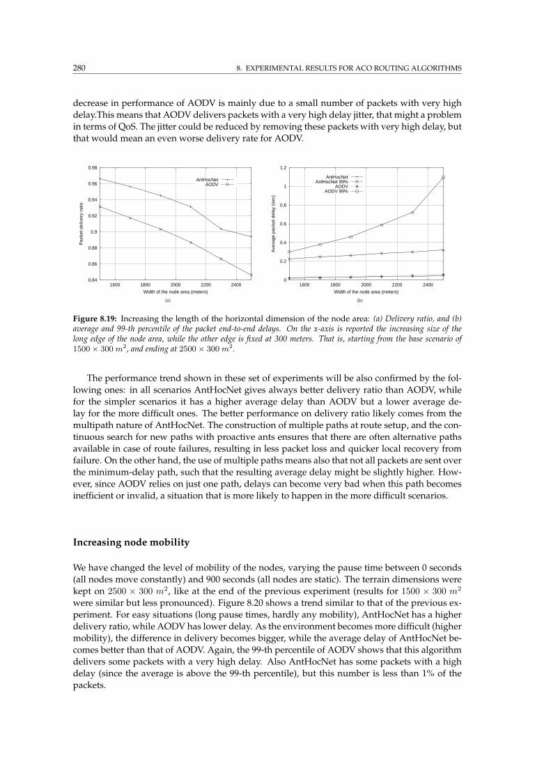
280 8. EXPERIMENTAL RESULTS FOR ACO ROUTING ALGORITHMS
decrease in performance of AODV is mainly due to a small number of packets with very high
delay.This means that AODV delivers packets with a very high delay jitter, that might a problem
in terms of QoS. The jitter could be reduced by removing these packets with very high delay, but
that would mean an even worse delivery rate for AODV.
0.84
0.86
0.88
0.9
0.92
0.94
0.96
0.98
1600 1800 2000 2200 2400
Pac
ket d
eliv
ery
ratio
Width of the node area (meters)
AntHocNetAODV
(a)
0
0.2
0.4
0.6
0.8
1
1.2
1600 1800 2000 2200 2400
Ave
rage
pac
ket d
elay
(se
c)
Width of the node area (meters)
AntHocNetAntHocNet 99%
AODVAODV 99%
(b)
Figure 8.19: Increasing the length of the horizontal dimension of the node area: (a) Delivery ratio, and (b)average and 99-th percentile of the packet end-to-end delays. On the x-axis is reported the increasing size of thelong edge of the node area, while the other edge is fixed at 300 meters. That is, starting from the base scenario of1500× 300 m2, and ending at 2500× 300 m2.
The performance trend shown in these set of experiments will be also confirmed by the fol-
lowing ones: in all scenarios AntHocNet gives always better delivery ratio than AODV, while
for the simpler scenarios it has a higher average delay than AODV but a lower average de-
lay for the more difficult ones. The better performance on delivery ratio likely comes from the
multipath nature of AntHocNet. The construction of multiple paths at route setup, and the con-
tinuous search for new paths with proactive ants ensures that there are often alternative paths
available in case of route failures, resulting in less packet loss and quicker local recovery from
failure. On the other hand, the use of multiple paths means also that not all packets are sent over
the minimum-delay path, such that the resulting average delay might be slightly higher. How-
ever, since AODV relies on just one path, delays can become very bad when this path becomes
inefficient or invalid, a situation that is more likely to happen in the more difficult scenarios.
Increasing node mobility
We have changed the level of mobility of the nodes, varying the pause time between 0 seconds
(all nodes move constantly) and 900 seconds (all nodes are static). The terrain dimensions were
kept on 2500 × 300 m2, like at the end of the previous experiment (results for 1500 × 300 m2
were similar but less pronounced). Figure 8.20 shows a trend similar to that of the previous ex-
periment. For easy situations (long pause times, hardly any mobility), AntHocNet has a higher
delivery ratio, while AODV has lower delay. As the environment becomes more difficult (higher
mobility), the difference in delivery becomes bigger, while the average delay of AntHocNet be-
comes better than that of AODV. Again, the 99-th percentile of AODV shows that this algorithm
delivers some packets with a very high delay. Also AntHocNet has some packets with a high
delay (since the average is above the 99-th percentile), but this number is less than 1% of the
packets.
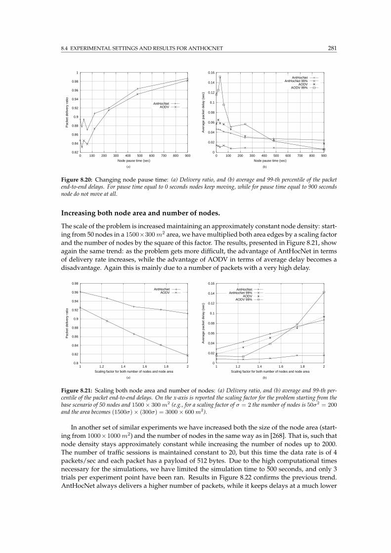
8.4 EXPERIMENTAL SETTINGS AND RESULTS FOR ANTHOCNET 281
0.82
0.84
0.86
0.88
0.9
0.92
0.94
0.96
0.98
1
0 100 200 300 400 500 600 700 800 900
Pac
ket d
eliv
ery
ratio
Node pause time (sec)
AntHocNetAODV
(a)
0
0.02
0.04
0.06
0.08
0.1
0.12
0.14
0.16
0 100 200 300 400 500 600 700 800 900
Ave
rage
pac
ket d
elay
(se
c)
Node pause time (sec)
AntHocNetAntHocNet 99%
AODVAODV 99%
(b)
Figure 8.20: Changing node pause time: (a) Delivery ratio, and (b) average and 99-th percentile of the packetend-to-end delays. For pause time equal to 0 seconds nodes keep moving, while for pause time equal to 900 secondsnode do not move at all.
Increasing both node area and number of nodes.
The scale of the problem is increasedmaintaining an approximately constant node density: start-
ing from 50 nodes in a 1500×300m2 area, we have multiplied both area edges by a scaling factor
and the number of nodes by the square of this factor. The results, presented in Figure 8.21, show
again the same trend: as the problem gets more difficult, the advantage of AntHocNet in terms
of delivery rate increases, while the advantage of AODV in terms of average delay becomes a
disadvantage. Again this is mainly due to a number of packets with a very high delay.
0.8
0.82
0.84
0.86
0.88
0.9
0.92
0.94
0.96
0.98
1 1.2 1.4 1.6 1.8 2
Pac
ket d
eliv
ery
ratio
Scaling factor for both number of nodes and node area
AntHocNetAODV
(a)
0
0.02
0.04
0.06
0.08
0.1
0.12
0.14
0.16
1 1.2 1.4 1.6 1.8 2
Ave
rage
pac
ket d
elay
(se
c)
Scaling factor for both number of nodes and node area
AntHocNetAntHocNet 99%
AODVAODV 99%
(b)
Figure 8.21: Scaling both node area and number of nodes: (a) Delivery ratio, and (b) average and 99-th per-centile of the packet end-to-end delays. On the x-axis is reported the scaling factor for the problem starting from thebase scenario of 50 nodes and 1500× 300 m2 (e.g., for a scaling factor of σ = 2 the number of nodes is 50σ2 = 200and the area becomes (1500σ)× (300σ) = 3000× 600 m2).
In another set of similar experiments we have increased both the size of the node area (start-
ing from 1000×1000m2) and the number of nodes in the same way as in [268]. That is, such that
node density stays approximately constant while increasing the number of nodes up to 2000.
The number of traffic sessions is maintained constant to 20, but this time the data rate is of 4
packets/sec and each packet has a payload of 512 bytes. Due to the high computational times
necessary for the simulations, we have limited the simulation time to 500 seconds, and only 3
trials per experiment point have been ran. Results in Figure 8.22 confirms the previous trend.
AntHocNet always delivers a higher number of packets, while it keeps delays at a much lower
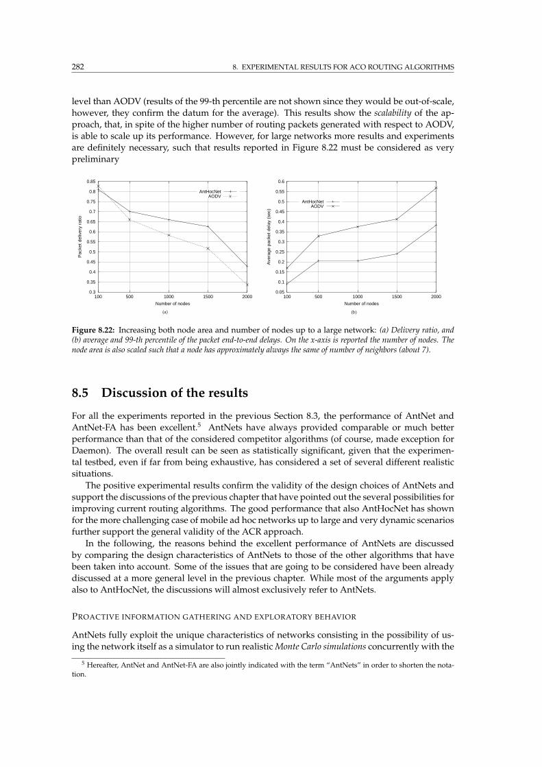
282 8. EXPERIMENTAL RESULTS FOR ACO ROUTING ALGORITHMS
level than AODV (results of the 99-th percentile are not shown since they would be out-of-scale,
however, they confirm the datum for the average). This results show the scalability of the ap-
proach, that, in spite of the higher number of routing packets generated with respect to AODV,
is able to scale up its performance. However, for large networks more results and experiments
are definitely necessary, such that results reported in Figure 8.22 must be considered as very
preliminary
0.3
0.35
0.4
0.45
0.5
0.55
0.6
0.65
0.7
0.75
0.8
0.85
100 500 1000 1500 2000
Pac
ket d
eliv
ery
ratio
Number of nodes
AntHocNetAODV
(a)
0.05
0.1
0.15
0.2
0.25
0.3
0.35
0.4
0.45
0.5
0.55
0.6
100 500 1000 1500 2000
Ave
rage
pac
ket d
elay
(se
c)
Number of nodes
AntHocNetAODV
(b)
Figure 8.22: Increasing both node area and number of nodes up to a large network: (a) Delivery ratio, and(b) average and 99-th percentile of the packet end-to-end delays. On the x-axis is reported the number of nodes. Thenode area is also scaled such that a node has approximately always the same of number of neighbors (about 7).
8.5 Discussion of the results
For all the experiments reported in the previous Section 8.3, the performance of AntNet and
AntNet-FA has been excellent.5 AntNets have always provided comparable or much better
performance than that of the considered competitor algorithms (of course, made exception for
Daemon). The overall result can be seen as statistically significant, given that the experimen-
tal testbed, even if far from being exhaustive, has considered a set of several different realistic
situations.
The positive experimental results confirm the validity of the design choices of AntNets and
support the discussions of the previous chapter that have pointed out the several possibilities for
improving current routing algorithms. The good performance that also AntHocNet has shown
for the more challenging case of mobile ad hoc networks up to large and very dynamic scenarios
further support the general validity of the ACR approach.
In the following, the reasons behind the excellent performance of AntNets are discussed
by comparing the design characteristics of AntNets to those of the other algorithms that have
been taken into account. Some of the issues that are going to be considered have been already
discussed at a more general level in the previous chapter. While most of the arguments apply
also to AntHocNet, the discussions will almost exclusively refer to AntNets.
PROACTIVE INFORMATION GATHERING AND EXPLORATORY BEHAVIOR
AntNets fully exploit the unique characteristics of networks consisting in the possibility of us-
ing the network itself as a simulator to run realisticMonte Carlo simulations concurrently with the
5 Hereafter, AntNet and AntNet-FA are also jointly indicated with the term “AntNets” in order to shorten the nota-tion.
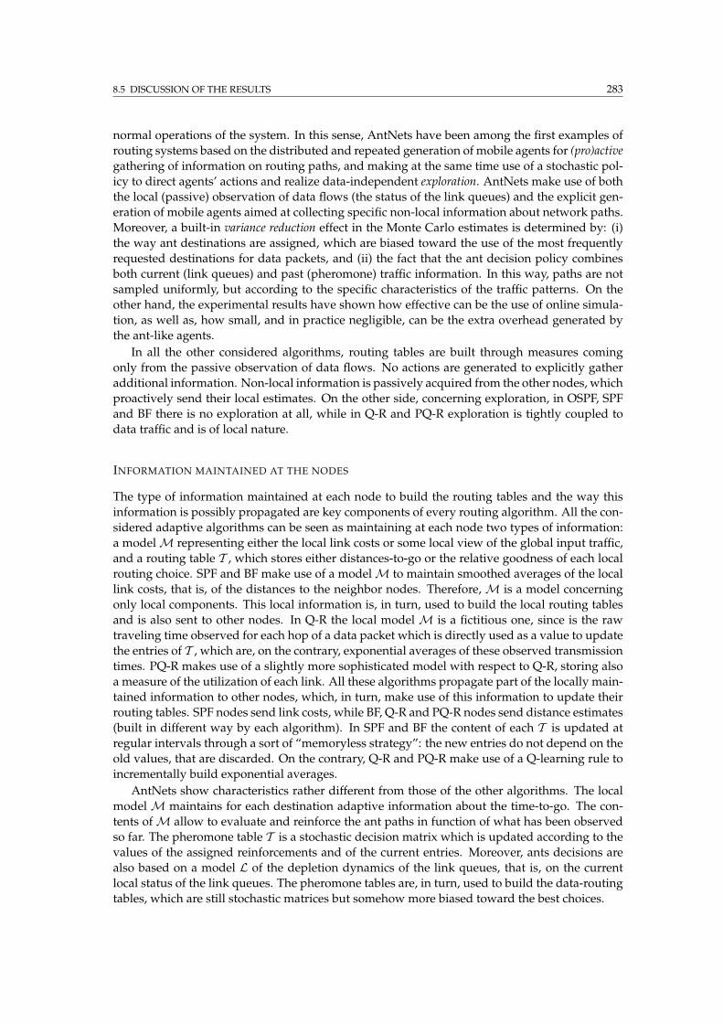
8.5 DISCUSSION OF THE RESULTS 283
normal operations of the system. In this sense, AntNets have been among the first examples of
routing systems based on the distributed and repeated generation of mobile agents for (pro)active
gathering of information on routing paths, and making at the same time use of a stochastic pol-
icy to direct agents’ actions and realize data-independent exploration. AntNets make use of both
the local (passive) observation of data flows (the status of the link queues) and the explicit gen-
eration of mobile agents aimed at collecting specific non-local information about network paths.
Moreover, a built-in variance reduction effect in the Monte Carlo estimates is determined by: (i)
the way ant destinations are assigned, which are biased toward the use of the most frequently
requested destinations for data packets, and (ii) the fact that the ant decision policy combines
both current (link queues) and past (pheromone) traffic information. In this way, paths are not
sampled uniformly, but according to the specific characteristics of the traffic patterns. On the
other hand, the experimental results have shown how effective can be the use of online simula-
tion, as well as, how small, and in practice negligible, can be the extra overhead generated by
the ant-like agents.
In all the other considered algorithms, routing tables are built through measures coming
only from the passive observation of data flows. No actions are generated to explicitly gather
additional information. Non-local information is passively acquired from the other nodes, which
proactively send their local estimates. On the other side, concerning exploration, in OSPF, SPF
and BF there is no exploration at all, while in Q-R and PQ-R exploration is tightly coupled to
data traffic and is of local nature.
INFORMATION MAINTAINED AT THE NODES
The type of information maintained at each node to build the routing tables and the way this
information is possibly propagated are key components of every routing algorithm. All the con-
sidered adaptive algorithms can be seen as maintaining at each node two types of information:
a modelM representing either the local link costs or some local view of the global input traffic,
and a routing table T , which stores either distances-to-go or the relative goodness of each local
routing choice. SPF and BF make use of a modelM to maintain smoothed averages of the local
link costs, that is, of the distances to the neighbor nodes. Therefore,M is a model concerning
only local components. This local information is, in turn, used to build the local routing tables
and is also sent to other nodes. In Q-R the local modelM is a fictitious one, since is the raw
traveling time observed for each hop of a data packet which is directly used as a value to update
the entries of T , which are, on the contrary, exponential averages of these observed transmission
times. PQ-R makes use of a slightly more sophisticated model with respect to Q-R, storing also
a measure of the utilization of each link. All these algorithms propagate part of the locally main-
tained information to other nodes, which, in turn, make use of this information to update their
routing tables. SPF nodes send link costs, while BF, Q-R and PQ-R nodes send distance estimates
(built in different way by each algorithm). In SPF and BF the content of each T is updated at
regular intervals through a sort of “memoryless strategy”: the new entries do not depend on the
old values, that are discarded. On the contrary, Q-R and PQ-R make use of a Q-learning rule to
incrementally build exponential averages.
AntNets show characteristics rather different from those of the other algorithms. The local
modelM maintains for each destination adaptive information about the time-to-go. The con-
tents ofM allow to evaluate and reinforce the ant paths in function of what has been observed
so far. The pheromone table T is a stochastic decision matrix which is updated according to the
values of the assigned reinforcements and of the current entries. Moreover, ants decisions are
also based on a model L of the depletion dynamics of the link queues, that is, on the current
local status of the link queues. The pheromone tables are, in turn, used to build the data-routing
tables, which are still stochastic matrices but somehow more biased toward the best choices.
284 8. EXPERIMENTAL RESULTS FOR ACO ROUTING ALGORITHMS
It is apparent that AntNets make use of a richer repertoire of information than the other
algorithms: (i) adaptive probabilistic models for distance estimates and to score the relative
goodness of each local choice, (ii) a simple model to capture the instantaneous state of the link
queues, (iii) a stochastic decision matrix for both data and ants routing. Each node in AntNets
is an actor-critic agent, learning on the basis of a wise balance between long- and short-term
estimates, in order to cope with the intrinsic variability of the input traffic. The use of several
components at each node has also the great advantage of reducing the criticality of each of these
components, since a sort of task distribution happens. In some sense, AntNets’ architecture is
not only using richer information but is also more robust with respect to those of the considered
competitors.
STOCHASTIC MULTIPATH ROUTING BASED ON PHEROMONE TABLES
All the tested algorithms but AntNets use a deterministic routing policy. More in general, AntNets
are the only algorithms really relying on the use of stochastic components. It has already dis-
cussed the fact that stochastic policies seem in general to be more appropriate to deal with non-
Markov, non-stationary problems. In AntNets, being based on proactiveMonte Carlo simulation
(the ants), stochasticity is at the core of the mechanisms for building the routing tables. But what
makes AntNets even more different from the other algorithms is the combined effect of using
different stochastic matrices to route ants and data. In this way, the ants have a built-in explo-
ration component that allow them to explore new routes using the ant-routing tables, while at
the same time, data packets make use of the data-routing tables, exploiting the best of the paths
discovered so far. None of the other considered algorithms keep on separate levels exploration
and exploitation. Actually, none of them really do exploration.
The use of a stochastic policy to route data packets result in a better distribution of the traffic
load over different paths, with a resulting better utilization of the resources and automatic load
balancing (the experiments with SimpleNet well show this fact). In this sense, AntNets are the
only algorithms which implement multipath routing. Data packets of a same session are con-
currently spread over multiple paths, if there are several equally good possible paths that can
be used. Moreover, AntNets do not have to face the problem of deciding a priori how many
paths have to be used. Since a relative goodness is assigned to every local choice, the chosen
transformation function of Equation 7.10 and the random selection mechanism of a next hop
automatically select the appropriate number of paths that will be actually used by data packets.
On the other hand, since every choice is locally scored by means of pheromone (and status of
link queues) and this score is proactively and repeatedly refreshed with some non null proba-
bility, even those paths that are not actually used by data are made available and can be used in
case of sudden congestion along the best paths, and/or in case of failure.
The fact that a bundle of paths is made available and scored by the ants, such that it can be
used for both multipath and backup routing is quite important to explain the good performance
shown by AntHocNet over AODV. The construction of multiple paths at route setup, and the
continuous search for new paths with proactive ants ensures that there are often alternative
paths available in case of route failures, resulting in less packet loss and in the higher delivery
ratio shown by AntHocNet in all the experiments. Moreover, local repair of paths after link
failures is made easier and quicker by the presence of the presence of multiple paths. On the
other hand, AntHocNet has a higher average delay than AODV for the simpler scenarios, but
a lower average delay for the more difficult ones (while results are always usually better if the
99-th percentile is considered). Again, this is in line with the multipath nature of AntHocNet:
since it uses different paths simultaneously, not all packets are sent over the shortest path, and so
the average delay will be slightly higher. On the other hand, since AODV relies on just one path,
delays can become very bad when this path becomes inefficient or invalid. This is especially

8.5 DISCUSSION OF THE RESULTS 285
likely to happen in difficult scenarios, with longer paths, lower node density or higher mobility,
rather than in the dense and relatively easy base scenario.
Concerning the contents of the routing tables, while AntNets maintains probabilistic measures
of the relative goodness of the local choices, all the other algorithms maintain for each choice a dis-
tance estimate to the destinations. The main difference consists in the fact that distance values are
absolute values, while the AntNets’ goodness measures are only relative values. For instance,
the values in the routing table of BF say that passing by neighbor n the distance to d is tn seconds,
while passing bym is tm seconds. This is quite different from what happens in AntNets, whose
data-routing table contains [0, 1] normalized entries like τnd and τmd that indicate the relative
goodness of choosing the route through m with respect to the route through n. On the other
hand, AntNets maintain estimates for the expected and best traveling times toward the destina-
tions from the current node in the modelM. However, distances are calculated considering the
whole set of neighbors, and not separately for each neighbor.
Under rapid traffic fluctuations, it might result quite hard to keep track for each neighbor
of the precise absolute distances toward the destinations of interest (as well as misleading con-
clusions can be easily drawn as shown in Subsection 7.1.4). On the other hand, is expected to
be more robust to deal with only relative measure of goodness assigned on the basis of all the
sampled information available, which is the approach followed in AntNets.
Another advantage of using normalized goodness values instead of absolute distances, con-
sists in the possibility of exploiting the arrival rate of the ants as a way to assign implicit rein-
forcements to the sampled paths. In fact, after the arrival of a backward ant, the routing table is
always updated, kicking up the path that has been followed by an amount that depends on both
the quality of the path and its estimated goodness. It is not obvious how the same effect could
be obtained by using routing tables containing distance estimates. In fact, in this case each new
sampled value of a traveling time would have to be added to the statistical estimate, that would
then oscillate around its expected value without inducing an arrival-dependent cumulative ef-
fect.
It is interesting to remark that the use of probabilistic routing tables whose entries are learned
in an adaptive way by changing on positive feedback and ignoring negative feedback, is reminis-
cent of older automata approaches to routing in telecommunication networks, alreadymentioned
in the previous chapters. In these approaches, a learning automaton is usually placed on each
network node. An automaton is defined by a set of possible actions and a vector of associated
probabilities, a continuous set of inputs and a learning algorithm to learn input-output associ-
ations. Automata are connected in a feedback configuration with the environment (the whole
network), and a set of penalty signals from the environment to the actions is defined. Routing
choices and modifications to the learning strategy are carried out in a probabilistic way and ac-
cording to the network conditions (e.g., see [334, 331]). The main difference lies in the fact that in
AntNet the ants are part of the environment itself, and they actively direct the learning process
towards the most interesting regions of the search space. That is, the whole environment plays
a key, active role in learning good state-action pairs, while learning automata essentially learn
only by induction.
ROBUSTNESS TO WRONG ESTIMATES
AntNets do not propagate local estimates to other nodes, as all the other algorithms do. The
statistical estimates and the routing table maintained at each node are updated after each ant
experiment without relying on any form of estimate bootstrapping. AntNets rely on pure Monte
Carlo sampling and updates. Each ant experiment affects only the estimates and the routing
table entries relative to the nodes visited by the ant, and local information is updated on the basis
of the “global” information collected by traveling ants along the path, implicitly reducing in this
286 8. EXPERIMENTAL RESULTS FOR ACO ROUTING ALGORITHMS
way the variance in the local estimates. All these characteristics make AntNets particularly
robust to wrong or out-of-date estimates. The information associated to each ant experiment
has a limited impact. If this characteristic can be a disadvantage under conditions of traffic
stationarity, it is an advantage under the more usual conditions of non-stationarity.
On the contrary, in all the other algorithms local estimates (of either link costs or distances)
are propagated to other nodes and might affect the decisions concerning all the different des-
tinations. Accordingly, an estimate which is wrong in some sense, is propagated overall the
network, and can have a globally negative impact. How bad this is for the algorithm perfor-
mance depends on how long the effect of the wrong estimate stay in the network. In particular,
for SPF and BF this is a function of frequency updates and of the propagation time throughout
the network, while for Q-R and PQ-R is a function of the learning parameters.
The issue of information bootstrapping in BF, Q-R, PQ-R and AntNets can be considered un-
der a more general perspective. In fact, as it has been already pointed out, AntNets are a sort
of parallel replicated Monte Carlo systems. As it has been shown by Singh and Sutton (1996),
a first-visit Monte Carlo simulation system (only the first visit to a state is used to estimate its
value during a trial) is equivalent to a batch temporal difference (TD) [413] method with replacing
traces and decay parameter λ = 1. In some sense, TD(1) is a pathological case of the TD class of
algorithms, since its results are the same obtained by a first-visit Monte Carlo, that is, without
any form of bootstrapping. The advantage of TD(1) overMonte Carlo is the fact that it can be run
as an online method [414, Chapter 7]. Although AntNets can be seen as first-visit Monte Carlo
simulation systems, there are some important differences with the type of Monte Carlo consid-
ered by Singh and Sutton and, more in general, by other works in the field of reinforcement
learning. The differences are mainly due to the differences in the characteristic of the considered
classes of problems. In AntNets, outcomes of experiments are both used to update local models
able to capture the global network state, which is only partially observable, and to generate a
sequence of stochastic policies. On the contrary, in the Monte Carlo system considered by Singh
and Sutton, the outcomes of the experiments are used to compute reduced maximum-likelihood
estimates of the expected mean and variance of the states’ returns (i.e., the total cost or payoff
following the visit of a state) of a Markov process. Actually, batch Monte Carlo methods learn
the estimates that minimize the mean-squared error on the used training set, while, for example,
batch TD(0) methods find the maximum-likelihood estimates for the parameters of the under-
lying Markov process [414, Page 144]. In spite of the differences between AntNet and TD(1),
the weak parallel with TD(λ) methods is rather interesting, and it allows to compare some of
the characteristics of AntNets with those of BF, Q-R and PQ-R by reasoning within the TD class
of algorithms. In fact, BF, Q-R and PQ-R are TD methods. In particular, Q-R and PQ-R, which
propagate the estimation information only one step back, are precisely distributed versions of
the TD(0) class of algorithms. They could be transformed into generic TD(λ), 0 ≥ λ < 1, by
transmitting backward to all the nodes previously visited by the data packet, the information
collected by the routing packet generated after each data hop. Of course, this would greatly in-
crease the routing traffic generated, because it has to be done after each hop of each data packet,
making the approach at least very costly, if feasible at all.
In general, using temporal differences methods in the context of routing presents an impor-
tant problem: the key condition of the method, the self-consistency between the estimates of
successive states, that is, the application of the Bellman’s principle, may not be strictly satisfied
in the general case. This is due to the fact that (i) the dynamics at each node are related in a
highly non-linear way to the dynamics of all its neighbors, (ii) the traffic process evolves concur-
rently over all the nodes, and (iii) there is a recursive interaction between the traffic patterns and
the control actions (that is, the modifications of the routing tables). According to these facts, the
nodes cannot be correctly seen as the states of a Markov process, therefore, the assumptions for
the effective application of TD methods whose final outcomes are based on information boot-
8.6 SUMMARY 287
strapping are not met. In this sense, the poor performance of TD(0)-like algorithms as Q-R and
PQ-R in case of highly non-stationary routing problems can be better understood. On the con-
trary, being AntNets a sort of batch TD(1) methods, not relying on information bootstrapping,
they can be more safely applied in these cases. Although, in case of quasi-stationarity, bootstrap-
ping methods are expected to be more effective and to converge more quickly.
UPDATE FREQUENCY OF THE ROUTING TABLES
In BF and SPF the frequency according to which routing information is transmitted to the other
nodes plays a major role concerning algorithm performance. This is particularly true for BF,
which maintains at each node only an incomplete representation of the network status and
topology. Unfortunately, the “right” frequency for sending routing information is problem-
dependent, and there is no straightforward way to make it adaptive, while, at the same time,
avoiding large oscillations (as is confirmed by the early attempts in both ARPANET and Inter-
net). In Q-R and PQ-R, routing tables updating is data driven: only the Q-values associated to
the neighbor nodes visited by data packets are updated. Although this is a reasonable strategy,
given that the exploration of new routes (by using data packets) could cause undesired delays
to data, it causes long delays before discovering new good routes, and is a major handicap in a
domain in which good routes could change all the time. In OSPF routing tables are practically
never updated: link costs have been assigned on the basis of the physical characteristics of the
links. This lack of an adaptive metric is the main reason of the poor performance of OSPF, as it
has been already remarked.
AntNets, from one side do not have the exploration problems of Q-R and PQ-R, since they
make use of simulation packets to explore new routes, from the other side, they do not have the
same critical dependency of BF and SPF from the frequency for sending routing information. In
fact, from the experiments carried out, AntNets have shown to be robust to changes in the ants’
generation rate: for a wide range of generation rates, rather independent of the network size,
the algorithm is able to provide very good performance, while, at the same time, the generated
routing overhead is in practice negligible also for considerable amount of generated ant agents.
8.6 Summary
In this chapter we have reported an extensive set of experimental results based on simulation
about the performance of AntNet, AntNet-FA, and AntHocNet.
Concerning AntNet and AntNet-FA, to which the majority of results refer to, in order to
provide significance to our studies, we have investigated several different traffic patterns and
levels of workload for six different types of networks both modeled on real-world instances and
artificially designed. The performance of our algorithms have been compared to those of six
other algorithms representative of state-of-the-art of both static and adaptive routing algorithms.
The performance showed by AntNet and AntNet-FA are excellent. Under all the considered
situations they clearly outperformed the competitor algorithms. In the case of low and quasi-
static input traffic, algorithms’ performance is quite similar, and has not been showed here.
On the other hand, AntHocNet has been compared only to AODV, which is however the cur-
rently most popular state-of-the-art algorithm for MANETs. We investigated the behavior of the
algorithms for a range of different situations in terms of number of nodes, node mobility, and
node density. We also briefly investigated the behavior in large networks (up to 2000 nodes). In
general, in all scenarios AntHocNet performed comparably or better than AODV. In particular, it
always gave better delivery ratio than AODV. Concerning delay, it had a slightly higher average
delay than AODV for the simpler scenarios (high density and short paths) but a lower aver-
age delay for the more difficult ones. While when considering the 99-th percentile for delays,
288 8. EXPERIMENTAL RESULTS FOR ACO ROUTING ALGORITHMS
AntHocNet had always better performance. The better performance on delivery ratio likely re-
sults from the multipath nature of AntHocNet that ensures that there are often alternative paths
available in case of route failures, resulting in less packet loss and quicker local recovery from
failure. On the other hand, the use of multiple paths means also that not all packets are sent over
the minimum-delay path, such that the resulting average delay might be slightly higher. How-
ever, since AODV relies on just one path, delays can become very bad when this path becomes
inefficient or invalid, as it might likely be the case in the more difficult scenarios. The good
performance also for large networks are promising regarding the scalability of the approach.
Even if it is not really possible to draw final conclusions, it is clear that we have at least
good indications that the general ACO ideas, once applied to distributed and highly dynamic
problems can be indeed very effective. In the last section of the chapter we have (re)discussed
the major design characteristics of AntNet and AntNet-FA, which have been directly inherited
from the ACO metaheuristic, and we have pointed out why and under which conditions these
characteristics are possibly an advantage with respect to those of other adaptive approaches. In
particular, the use of: active information gathering and path exploration, stochastic components,
and both local and non-local (brought by the ants) information, are the most distinctive and ef-
fective aspects of AntNet, AntNet-FA, and AntHocNet design, and, more in general, of instances
of ACR. These algorithms can automatically provide multipath routing with an associated load
balancing. More in general, a bundle of paths is adaptively made available and maintained,
with each path associated to a relative measure of goodness (the pheromone), such that the best
paths can be used for actual data routing, while the less good ones can be used as backup paths
in case of need.
We have shown that the algorithms are quite robust to internal parameter settings and in
particular to the ant generation rate, as well as to possible ant failures. Moreover, the study
on routing overhead for AntNet has shown that the actual impact of the ant-like agents can be
made quite negligible while at the same time still providing good performance, at least in small
wired networks. Clearly much more care in the ant generation and spreading must be taken in
the case of mobile ad hoc networks. And in a sense, this is one of the issues critically affecting
the performance of the algorithm in this case.
Part III
Conclusions


CHAPTER 9
Conclusions and future work
9.1 Summary
The main goals of thesis have been the definition and study of the Ant Colony Optimization
metaheuristic, and the design, implementation, and testing of ACO instances for routing tasks
in telecommunication networks. The ACO metaheuristic is a multi-agent framework for combi-
natorial optimization tasks that finds its root in the pheromone-mediated shortest path behavior
of ant colonies. The design of optimization algorithms based on the ACO metaheuristic has
gained a good level of popularity in recent years. This is witnessed by the number of applica-
tions discussed in Chapter 5, most of which perform in their domain of interest comparably or
better than state-of-the-art algorithms, as well as by the number of ACO-related scientific events
(workshops, special issues, books), as it has been pointed out in the Introduction. The interest
that ACO has attracted so far in the scientific community asked for a complete overview on, as
well as for an initial systematization of, the subject. This is what has been done in this thesis,
which has been an in-depth journey through the ACOmetaheuristic, during which we have de-
fined ACO and tried to get a clear understanding of its potentialities, limits, and relationships
with other frameworks.
Through the first part of the thesis we discussed the ACO’s genesis and biological context
of inspiration (Chapter 2), identified the mathematical context of reference (Chapter 3), pro-
vided definitions of ACO and analyzed its properties (Chapter 4), reviewedmost of the practical
implementations (Chapter 5), and selected a specific domain of application (routing problems
in telecommunication networks) as the most promising, innovative, and appropriate one to be
tackled by ACO algorithms (Summary of Chapter 5). In the second part of the thesis, we first dis-
cussed the characteristics of routing problems and of current approaches to routing (Chapter 6),
then we proposed four novel algorithms (AntNet, AntNet-FA, AntNet+SELA, AntHocNet) for
adaptive routing in different types of networks, and the definition of Ant Colony Routing (ACR),
a framework for adaptive control in networked environments which extends and generalizes
ACO by making use of both learning and ant-like agents (Chapter 7). The effectiveness of the
proposed algorithms, and, more in general, of the ACO approach for routing, has been validated
by the excellent performance shown by the algorithms through extensive simulation studies in
which they were compared to state-of-the-art algorithms (Chapter 8).
In the first part of the thesis we tried to cover most of the aspects that are relevant for ACO
in order to provide a complete picture that is intended to serve also as reference and inspiration
for researchers from different domains interested in ACO, and, more in general, in the design
of ant-inspired optimization algorithms. On the other hand, the second part has provided a
comprehensive discussion on the theoretical and practical issues concerning the application of
ACO to the specific domain of control problems in telecommunication networks.
We defined ACO adopting the language of sequential decision processes (introduced in
Chapter 3), that is, viewing each ant-like agent as an independent sequential decision process
aimed at constructing a feasible solution to the problem at hand by selecting solution compo-
nents one-at-a-time. In this way a great emphasis has been put on the pheromone variables,
292 9. CONCLUSIONS AND FUTURE WORK
that are the distributed parameters of the stochastic decision policy of the ants and serve for
the purpose of estimating the goodness of having a specific component in the solution condi-
tionally to the fact some other components are already included into the constructing solution
(more specifically, conditionally to the last included component). The values of the pheromone
variables are the result of a continual process of collective learning happening in the form of
a generalized policy iteration based in turn on the outcomes of the Monte Carlo sampling of
solutions realized by the ants. The characteristics of the pheromone model define the repre-
sentation of the problem available to the ant agents for the purpose of framing memory of the
single decisions issued so far and of the quality of the solutions they participated to. In turn, the
pheromone variables are used to take optimized decision exploiting the experience about the
solutions sampled so far. This characterization of the ACO metaheuristic is in accordance with
the original definition co-authored by the author in 1999 [147, 138, 137]. Nevertheless, it intro-
duced a slightly different language, corrected some aspects, provided some generalizations of it,
and allowed to highlight important connections between ACO and dynamic programming and
ACO and reinforcement learning. In particular, these logical connections allowed to get a clear
understanding of the critical role of the pheromone model, as well as of the intrinsic limitations
in the use of pheromone variables once compared to the use of complete information states,
since pheromone variables rely on the notion of phantasma, that is, a low-dimensional set of
state features. This new understanding allowed us to also propose a revised and extended def-
inition of the ACO’s pheromone variables that could partially overcome the limitations related
to the original definition (Section 4.4).
The first part of the thesis was rather theoretical and speculative, but at the same time pro-
vided also an extensive review of the main characteristics of most of the ACO applications to
combinatorial optimization problems (not falling in the class of online network problems). In
this way we gave a quite complete picture on both ACO’s theoretical properties and practical
implementation issues. With this knowledge in the hands, we could get a clear understanding
of the general potentialities and limits of ACO algorithms, and we could identify in adaptive
routing/control problems in telecommunication networks, rather than in classical static and cen-
tralized combinatorial problems, the most promising and innovative domain of application of
ACO’s ideas (Chapter 5). It is according to this conviction that the second, application-oriented
part of the thesis was entirely devoted to the study and application of ACO to routing problems
in telecommunication networks (clearly, this has not to be intended as a negative statement to-
ward the application of ACO to static and centralized optimization problem on absolute terms,
but rather as a sort of relative ranking between the two considered domains of application).
In Chapter 7 we proposed four algorithms for adaptive routing in different types of net-
work (wired networks providing best-effort and QoS routing, and mobile ad hoc networks). All
the algorithms have been designed according to the general ACO’s philosophy adapted to the
specificities of networked environments, that feature: online operations, fully distributed deci-
sion system, non-stationary input traffic, recursive interaction between routing decisions and
traffic patterns, and so on. We discussed (Chapters 6 and 7) in which sense ACO algorithms for
routing contain innovative and competitive aspects with respect to more classical and widely
used in routing approaches (e.g., ACO algorithms are fully adaptive, make use of active dis-
covery and gathering of non-local information, provide automatic load balancing and fast and
robust reactions to sudden changes by making available multiple choices at the nodes and by
adopting stochastic routing decisions, are robust to agent failures and/or incorrect behaviors,
etc.). Our theoretical expectations for good performance were fulfilled by the excellent exper-
imental results showed by the proposed algorithms, always performing comparably or better
than the considered state-of-the-art algorithms (Chapter 8). We were not interested in providing
with our algorithms just a proof-of-concept, but rather our purpose was to deliver state-of-the-
art performance under realistic assumptions and for an extensive set of scenarios. At this aim
9.2 GENERAL CONCLUSIONS 293
we payed special attention to the general experimental settings, to the characteristics of the sim-
ulators used for the experiments, and to the selection of the state-of-the-art algorithms used to
compare the performance of our algorithms against.
Encouraged by the brilliant performance, as well as by the number of works in the domain
of routing that have been designed after our and other ACO algorithms, we went further, and
defined the Ant Colony Routing framework (Chapter 7). That is, a meta-architecture and a
collection of ideas/strategies for the design of network routing (and, more in general, control)
algorithms. All the algorithms presented in the thesis can be seen as special instances of the ACR
framework. ACR specializes the general ACO’s ideas to the case of networks and at the same
time provides a generalization of these same ideas in the direction of integrating explicit learn-
ing and adaptive components into the design of ACO algorithms. In ACR the ant-like agents are
seen as non-local active perceptions (and effectors) explicitly issued by node managers, that are
the true controllers of the network. Each node manager is an autonomic reinforcement learning
agent that acts independently but socially to concur to the global optimization of the network
performance. It is expected to self-tune its internal parameters and behaviors in order to opti-
mize its performance, possibly via some learning process. ACR has defined the generalities of
a multi-agent society that is expected to be a meta-architecture of reference for the design and
implementation of fully autonomic routing systems, in accordance with the general organiza-
tion envisaged for autonomic systems in [250]. The formalization of ACR is still at a preliminary
stage, however, all the basic components that are considered as necessary to build a fully auto-
nomic systems are already part of ACR.
9.2 General conclusions
A Nature-inspired metaheuristic
Undoubtedly, part of the ACO’s popularity is due to the fact that it is aNature-inspired metaheuris-
tic with a quite simple and modular structure based on the use of ant-like agents and stigmergy.
That is, an optimization metaheuristic which promises to generate optimal or near-optimal solu-
tions on the basis of a recipe made of a set of possibly simple and computationally light agents,
that independently and repeatedly construct solutions according to a stochastic decision policy
locally dependent on pheromone variables. Part of the appeal of ACO precisely comes from this
expectation of generating extremely good solutions out of the simplicity of the main actors (the
ant-like agents) and from the collective and fully distributed learning activities in which they are
involved in, similarly to what happens in the case of real ant colonies (as discussed in Chapter 2).
ACO is probably the most successful example of so-called swarm intelligence [51, 249]: it is a
first step towards the ultimate objective of controlling the generation of complex behaviors from
simple and collective behaviors/learning relying only on local information. Nevertheless, in the prac-
tical application of the ACO framework, good solutions do not easily result from a simple/naive
design. In order to obtain reasonably good performance with respect to state-of-the-art algo-
rithms, ACO algorithms must be carefully designed in all their components as shown by the
review of ACO applications in Chapter 5. And even if it can be claimed that the ant-like agents
are usually quite simple, on the other hand each ant must be always complex enough to effi-
ciently construct a solution for the problem under consideration. Shortly, we are still far away
from the dreamed situation in which we need to define just few simple rules, and complex be-
haviors efficiently result from the interaction of a number of simple elements. Nevertheless, as
a matter of fact, the basic characteristics of ACO are quite intriguing, and make the design of
an ACO algorithm a relatively straightforward task. These facts, together with the often excel-
lent experimental performance showed by ACO algorithms, are certainly behind the quite large
interest that ACO has attracted so far in the scientific community.
294 9. CONCLUSIONS AND FUTURE WORK
Use of memory and learning
The joint use of memory and learning by sampling is another of the most distinctive traits of ACO,
and another of the reasons behind its popularity as well as its efficacy. We stressed this aspect
of ACO across the thesis, proposing also an original reading of ACO in terms of sequential
decision processes and generalized policy iteration based on Monte Carlo learning (Chapter 4),
and highlighting ACO’s relationships with other learning and control frameworks (Chapter 3).
In general, the use of memory and learning to solve optimization tasks is attracting an increasing
interest in recent years (especially in the form of distribution estimation algorithms, as discussed
in Section 5.3), and ACO is undoubtedly one of the leading metaheuristics for what concerns the
application of these notions to combinatorial optimization.
How effective a strategy based on learning by sampling can be in the case of combinatorial
optimization is however not immediately clear, due to the lack of a topology of reference in com-
binatorial spaces. ACO represents a sort of empirical evidence that such a way of proceeding
can be fruitful. On the other hand, it is a matter of fact that the most effective heuristics for com-
binatorial problems are usually based on problem-specific procedures of local search that make
little or no use at all of learning strategies. A way of proceeding that seems to be particularly
effective consists in the design of hybrid algorithms, in which problem-specific local search pro-
cedures are included as Daemon procedures into the design of the ACO algorithm (or of other
learning-based algorithms, as in the case of the STAGE algorithm [55]). It is an empirical ev-
idence that the combined use of local search and ACO synergistically boosts the performance
of both components resulting in algorithms performing extremely well. It is said that ACO can
learn good starting points for the local search, as well as that ACO searches in neighborhoods that
are complementary with respect to local search (see also Appendix B). However, these empirical
evidences need to be supported by more precise results, both theoretical and experimental.
Pheromone models based on incomplete state information
In the design of an ACO algorithm a critical and sometimes conceptually rather difficult step
consists in the definition of the problem representation used by the ants to take decisions and
frame memory of generated solutions. That is, the transformation of the problem at hand into
a sequential decision problem, and the definition of the decision variables and of the way they get
updated after sampled solutions. The characteristics of the pheromone model used by the ant-like
agents greatly affect the final performance of the algorithm. After this step, even if several other
components still have to be chosen and properly tuned (e.g., the characteristics of the scheduling
of the ants, that directly affects the evaluation of the current policy), the design of the rest of the
algorithm is in general rather straightforward and reasonably good performance can be quite
easily obtained with little effort in parameter tuning. Nevertheless, because of inescapable com-
putational limits, the cardinality of the chosen pheromonemodel is always expected to represent
a low-cardinality projection of the set of the complete information states of the problem, which are
those used by an exact approach like dynamic programming (Chapters 3 and 4). This means that
the ant agents have to rely on incomplete representations of the problem at the time of taking
optimized decisions.
This information loss with respect to the fully informative state representation adopted by
dynamic programming has important negative consequences concerning finite-time conver-
gence and provided performance. In particular, it affects the fact that only asymptotic guar-
antees of convergence can be usually provided, which are of doubtful practical utility for combi-
natorial problems (Chapter 3), and the fact that state-of-the-art performance in the case of static
and offline combinatorial problems are usually obtained only when problem-specific Daemon
procedures of local search are included in the design of the algorithm.
9.2 GENERAL CONCLUSIONS 295
If part of the limitations in the ACOperformance can be easily explained by the fact that ACO
is actually a general-purpose metaheuristic, it is also true that the use of more state information
could be highly beneficial. It is to go in this direction that in Section 4.4 we proposed a revised
definition of both the derivation of the phantasma from the state and the way pheromone vari-
ables are used at decision time. According to the new definitions, the phantasma does not coin-
cide necessarily with one single component, but it can be made of any subset of state features,
dramatically increasing in this way the amount of retained state information. Nevertheless, this
direction is not free from problems, since more state information in the phantasma means an
increase in the number of phantasmata. That is, a way more complex learning problem to deal
with. An appropriate balance between the richer information at hand to take decisions and the
increased complexity to deal with must be necessarily found.
Design and tuning of ACO instances
In addition to the definition of the pheromonemodel, several other components must be defined
at the time of designing a new ACO algorithm (e.g., see Section 4.3). Among the most critical
ones are: the strategies for the scheduling of the ants, the form of the ant-routing table and decision
policy, and the strategies for the use of the sampled information to update pheromone variables.
The ant scheduling determines the level of evaluation of the current policy and/or the fre-
quency for gathering fresh information in online problems. The form of the ant-routing table
defines the balance between pheromone information, resulting from the collective ant learn-
ing, and heuristic information, resulting from either a priori knowledge or external processes.
The form of the decision policy defines the chosen balance between exploration and exploita-
tion during the phases of solution construction. Finally, the strategies for pheromone updating
determine which information is considered valuable and with which strength it has to bias sub-
sequent solution generations.
While all these components are expected to be more or less equally important, a proper
setting of the pheromone updating strategy seems to be one of the main keys to reach re-
ally good performance for static optimization problems. The empirical evidence seems to sug-
gest that the most effective strategies are those that update the policy parameters according
to some elitist selection that is, on the basis of only a restricted subset (typically the best ones)
of the solutions generated so far (e.g., this is the strategy adopted by ACS [140, 141, 184] and
MMAS [406, 407, 408, 404], that are among the best performing ACO implementations). The
rationale behind this is the fact that ACO does not make use of states as learning target. Ac-
cordingly, the information coming from solution sampling should be used for quickly spotting
which are those decisions that belongs to good solutions, and not, for instance, to try to build
good estimates of the expected values of single decisions, since these expected values would be
very noisy due to the fact that decisions are related to pairs of components and not to pairs of
states (see also Subsection 4.3.2). Therefore, a large part of the sampled solutions can be thrown
away, selecting only the best ones for pheromone updating. In this way, the single decisions
belonging to good solutions can be fixed, and bias for a while the processes of solution construc-
tion. Therefore, in practice, it seems rather important to be quite greedy towards good solutions,
letting the agents explore in depth the areas around the good solutions found, and possibly in
some sense moving toward another area when a new better/good solution is found.
In the case of telecommunication networks, the overall strategy for pheromone updating is
less critical than in the case of static problems. In fact, in these cases any ant sample of an end-to-
end delay can be quite safely used to update useful statistics (however, some care must be taken
also in these cases, as pointed out in Subsection 7.1.3.7). Way more important is the related is-
sued of the scheduling of the ant agents. More ants means more and up-to-date information, but
also increased overhead and routing-induced congestion. Finding a right balance between these
296 9. CONCLUSIONS AND FUTURE WORK
two opposite aspects is the key to get good performance, especially in bandwidth-constrained
networks like MANETs. ACR has explicitly pointed out the issue and suggested some general
strategies to deal with it. On the other hand, in static non-distributed problems the tendency
for ant scheduling consists in using few ants at each iteration. That is, choosing to get a very
incomplete evaluation of the current policy but at the same time updating the policy a consid-
erable number of times. However, so far there are no in-depth and general studies concerning
either the selection of the components of ACO algorithms or the values to assign to the basic
parameters.
Network control problems as the most suited to ACO’s characteristics
One of the theses of this dissertation is that ACO’s characteristics are indeed a good match in
particular for routing and, in general, control tasks in telecommunication networks, more than for
static and non-distributed combinatorial optimization problems (see Summary of Chapter 5 and
Chapters 6 and 7). In fact, for this wide class of problems of extremely practical and theoretical
importance, the multi-agent, distributed, and adaptive nature of the ACO architecture can be
fully exploited. Such that the design of ACO algorithms for adaptive network control is at
the same time: (i) extremely natural (the characteristics of the pheromone model are directly
dictated by the network structure and the ants are true mobile agents), (ii) innovativewith respect
to most of current state-of-the-art algorithms (ACO algorithms feature full adaptivity, active
information discovery by mobile agents, availability of multiple paths for routing and backup
actions, automatic load balancing, robustness to agent failures, use of stochastic components,
and so on), and (iii) successful, as showed by the impressive experimental results of extensive
simulation studies over a wide set of scenarios and types of network reported in Chapter 8.
Once compared to the application to classical static combinatorial optimization problems,
the application to online network problems presents several advantages: (a) better than state-
of-the-art performance can be obtained by genuine ACO implementations, without the need of
daemon components to boost up the performance, (b) the choice of an effective representation of the
problem at hand is not anymore a major problem, since it is naturally suggested by the intrinsic
characteristics of the environment: the network nodes are the decisions points (i.e., the solution
components) holding the pheromone tables, and each pheromone variable represents, for each
locally known final destination d and for each feasible next hop node n, the locally estimated
goodness of forwarding a data packet through nwhen its final destination is d, (c) the distributed
multi-agent architecture of ACO in the case of networks becomes a natural and effective way
of dealing with the problem, while it is more an abstraction than a real issue in the case of
non-distributed problems, (d) the implicit solution evaluation discussed in Subsection 4.3.3 and
Section 2.1 can be exploited at null cost, such that both the frequency of the ants and the explicit
evaluation of their paths can be used to update the pheromone tables, (e) the issue of convergence
in either finite or asymptotic time becomes of less practical importance, due to the fact that in
dynamic environments rather than convergence (that requires stationarity), it is more important
the ability of the algorithm to effectively adapt to the ever changing situations, and this is what ACO
ants do by repeated Monte Carlo sampling of paths and distributed updating of the routing
policy at the nodes, (f) while the use of memory and learning are not anymore truly innovative
ideas in the domain of combinatorial optimization, on the other hand, the characteristics of ACO
algorithms for routing tasks are significantly different and innovativewith respect to those of the
majority of the algorithms most in use, and appear to be good candidates to become building
blocks for the fully autonomic [250] and adaptive routing systems that will hopefully operate in
forthcoming active networks [420].
9.3 SUMMARY OF CONTRIBUTIONS 297
The challenge of Ant Colony Routing
The ACO routing algorithms that we defined and tested (AntNet, AntNet-FA, and AntHocNet),
showed excellent performance. More in general, the application of ACO to routing tasks has
gained some popularity, such that several implementations, most of them directly inspired by
our original work on AntNet, have appeared in literature (see also Section 7.4), and their perfor-
mance is usually quite good. We tried to identify the reasons behind this popularity, as well as
the common characteristics across the implementations that are behind the more than promis-
ing performance. This resulted in the definition of ACR as a general framework derived from
ACO for the design of routing (and control) algorithms for networked/distributed environments
(Chapter 7). Designing an algorithm in true accordance to the ACR guidelines is a challenging
task, but is at the same time the way toward the realization of truly autonomic and optimized sys-
tems for the online control of distributed environments. And we believe that this is the direction that
the design of networked computing systems will follow more and more in the coming years.
Such that, in order to build on top of the basic ACO ideas systems that can have impact and find
useful application also in the future, we hold the conviction that the way indicated by ACR is
the most promising and interesting one.
The challenge defined by ACR consists in the fact that it explicitly addresses the issues of the
scheduling of the ant-like agents, the definition of their internal characteristics, and the assign-
ment of the tasks they have to deal with. ACR proposes to view these issues in terms of adaptive
learning issues. The ACR’s nodemanagers are fully autonomic and adaptive reinforcement learn-
ing agents. Each node manager participate in the continual and collective optimization of the
global network performance by learning the local control policy. At this aim it makes use of
ant-like agents explicitly generated to support its local activities with non-local discovering and
monitoring of useful information. On the other hand, learning an effective control policy by
using the ant-like agents asks in turn for the adaptive learning of the scheduling strategies and
characteristics of these agents, as well as of the values of their internal parameters. That is, a sort
of hierarchical organization in two levels of learning.
ACR’s architecture specializes and at the same time generalizes that of ACO, pointing out
the need of integrating explicit learning components into the design of ACO algorithms. If this
way of proceeding can be seen as necessary in the case of online network problems to track the
non-stationarity and to deal with the problematics arising from the distributed architecture, it
can result useful also in the case of static problems. In fact, for instance, the scheduling and
the characteristics of the ant agents are directly related to the critical issues of partial evaluation
of the current policy and of exploration versus exploitation. More in general, if ACO has been
presented as a memory- and learning-based approach to combinatorial optimization, with ACR
we pointed out the need of introducing in ACO new components that learn how to learn.
9.3 Summary of contributions
The technical and conceptual contributions contained in the thesis are briefly discussed in the
following list that introduces the contributions on a per chapter basis.
Chapter 2 - This chapter has acknowledged the biological background of ACO. The main con-
tributions consist in the review and discussion of the biological literature related to ant colonies
shortest path behaviors, and in the abstraction and critical analysis of the main elements that
make these synergistic behaviors happening. We have also provided an original discussion on
the more general issue of self-organized behaviors in biological systems as the result of nonlin-
ear dynamics that can be modeled in the terms of stigmergic protocols of communication and
coordination among a number of “cheap” and concurrent agents. Artificial stigmergy itself has
298 9. CONCLUSIONS AND FUTURE WORK
been provided with a new definition and the notion of stigmergic variable (i.e., pheromone) has
been clarified. The “ant way”, as particular instance of stigmergic multi-agent modeling directly
derived from ant colony characteristics, has been informally defined.
Chapter 3 - In this rather long chapter we defined/introduced the formal tools and the basic
scientific background that we used to define and discuss ACO in the terms of a multi-agent
metaheuristic featuring solution construction, use of memory, repeated solution sampling, and
learning of the parameters of the construction policy over a small subspace. The overall original
outcome of the chapter consists in having put on a same logical line several different notions
coming from different domains (optimization, control, and reinforcement learning), disclosing
their connections, and extracting their general core properties in relation to combinatorial opti-
mization issues. The chapter (together with all the appendices from A to E) can be also seen as
a reasoned review of literature on heuristic, decision-based, and learning-based approaches to
combinatorial optimization.
There are also several specific technical contributions contained in the chapter: (i) the char-
acteristics of different abstract problem representations have been discussed and the notion of
solution component has been formally defined and put in relationship with problem representa-
tions given in terms of primitive, environment, and constraint sets, (ii) a formal definition and an
extensive analysis of construction methods for combinatorial optimization has been provided,
(iii) the relationship between construction methods and sequential decision processes and, in
turn, optimal control, has been pointed out, formalized, and discussed, (iv) the notion of con-
struction graph as a graphical tool to represent and reason on sequential decision processes has
been introduced and formally defined on the basis of a previous analysis of the properties of
the state graph of the process, (v) the notion of generating function of the construction graph
from the state graph has been formally defined and used to reason on the information loss and
visualization capabilities of a construction graph, (vi) the general characteristics of MDPs have
been discussed as well as the potential problems deriving from using a Markov model which is
based on state features rather than on the complete information states of the problem, (vii) the
notion of phantasma, as a function of state features, and used in ACO for the purpose of memory
and learning, has been formally introduced together with the phantasma representation graph,
which is equivalent to a generalization of the construction graph.
Among other minor original contributions contained in the chapter, there is a discussed re-
view of the general characteristics of value-based (i.e., based on Bellman’s equations) methods
versus policy search methods. In particular, the chapter considers the case of policy search
strategies based on the transformation of the original optimization problem in the problem of
learning on a set of policies defined over a low-dimensional parametric space. Which is pre-
cisely the strategy followed by ACO, with the pheromone array playing the role of learning
parameters.
Chapter 4 - The original contribution of this central chapter consists in the definition in two steps
of the ACOmetaheuristic and in the in-depth discussion of its characteristics. First, we provided
a formal description of the metaheuristic which is substantially conformal to that given in the
papers were ACO was first introduced by Dorigo, Di Caro, and Gambardella [147, 138]. In the
second step, we revised and extended the original definition for what concerns the characteris-
tics of the pheromone model and of the way pheromone variables are used at decision time.
The first definition contains several new aspects with respect to the original, published one,
and makes also use of a more formal and slightly different mathematical language (that de-
veloped in the previous Chapter 3) for the purpose of emphasizing the relationships between
ACO and the frameworks of sequential decision processes and control, and making explicit the
methodological and philosophical assumptions behind ACO as well as its potentialities and
limits. Among the newly introduced aspects, the definition is based on an explicit distinction
9.3 SUMMARY OF CONTRIBUTIONS 299
between feasibility and optimization of the quality of the solutions. At this purpose, we intro-
duced the use of the state graph for solution feasibility, and of the pheromone graph (which is
a phantasma representation graph) for framing memory of the sampled solutions in the form
of pheromone variables and taking optimized decisions in the sense of the quality of the so-
lution. In particular, the relationships between the fully informative but computationally un-
manageable state graph, and the much smaller but carrying incomplete information pheromone
graph, are highlighted and thoroughly discussed to disclose the true nature of pheromone vari-
ables as subsets of state features. The ACO’s definition given here introduces also the notion
of pheromone manager, as an autonomous component of the algorithm that regulates all the
activities of pheromone updating.
In the original definition, pheromone variables are associated to pairs (component, component)
such that the decision about the new component to include is issued conditionally to the fact that
another specific single component is already in the solution (and is possibly the last included
one). In the revised definition we extended and generalized the original pheromone model in
order to either increase the amount or improve the quality of the used pheromone information:
(i) pheromone variables are associated to pairs (phantasma, component), where the phantasma
can represent any set of state features, (ii) any aggregate of pheromone variables can be used at
decision time to assign the selection probability of a feasible component (in the previous case
only one variable was considered at a time).
Among the other contributions of the chapter there are extensive discussions of the ACO’s
characteristics, especially regarding the use of memory and learning. The connections and the
differences with dynamic programming, policy search, and Monte Carlo methods have been
also pointed out and discussed. The role of different design choices has been analyzed, focusing
in particular on the strategies for pheromone updating, which have been recognized as one of
the most critical components. In particular, the use of elitist strategies is invoked as the most
effective choice in this sense. On the other hand, the Metropolis-Hastings class of algorithms
has been suggested for use as harness of ACO algorithms, in order to provide general and at the
same time theoretically sound strategies for pheromone updating.
Chapter 5 - This chapter was mainly devoted to review current ACO implementations for com-
binatorial optimization problems (but not the applications to online network problems). There-
fore, its main contribution precisely consists of providing a quite comprehensive and up-to-date
overview of most of all the ACO algorithms implemented so far. Each algorithm is briefly ex-
plained, its most interesting features, design choices, and reported performance are discussed.
In particular, we highlighted the different choices adopted concerning problem representation
and pheromone model, strategies for pheromone updating, and the use or not of local search
and its relative impact on the algorithm performance when it is used.
The population-oriented nature of ACO algorithms makes them particularly suitable to par-
allel implementations, such that a number of parallel models and implementations have been
developed so far. We reviewed also these, suggesting a classification taxonomy based on the
different parallel computational models adopted, on the use or not of multiple colonies, and on
the way information is exchanged either among the colonies or among the ants.
In this chapter we also discussed similarities and differences between ACO and other related
optimization approaches. In particular, we identified in evolutionary and cultural algorithms,
rollout algorithms, cross-entropy, stochastic learning automata, and neural networks, the frame-
works that share the strongest similarities with ACO.
The chapter was concluded with a fundamental contribution of this thesis: with in the hands
the comprehensive review of applications and the outcomes of all the previous discussions about
general ACO’s characteristics, we argued that the application of ACO to online problems in
telecommunication networks is more sound, innovative, appealing, and in a sense, also “natu-
300 9. CONCLUSIONS AND FUTURE WORK
ral” and genuine, than that to classical static and centralized combinatorial optimization prob-
lems. Clearly, this did not mean that the application of ACO to this last class of problems is not
appropriate. In fact, the experimental results tell us that the application of ACO can indeed re-
sult in extremely good performance also in these cases. However, we pointed out some general
reasons to prefer, in purely relative terms, the application of ACO to dynamic network problems.
And in the second part of the thesis we tried to validate and fully support this view.
Chapter 6 - Similarly to Chapter 3, this chapter too was a sort of preparatory chapter that in-
troduced the terminology, the problems, and the general mathematical and algorithmic back-
ground related to routing in telecommunication networks. The contents of the chapter are com-
plemented by Appendix F, that reports about general characteristics of telecommunication net-
works (layered architectures, transmission technologies, delivered services, etc.).
Therefore, the main contributions of this chapter can be seen in the terms of providing a
high-level literature overview on routing issues, and, in particular, concerning adaptive and
multipath routing solutions versus static and single-path strategies. One of the original con-
tributions of this overview precisely consists in having pointed out both the good and the bad
aspects of popular routing paradigms (optimal routing and shortest-path routing) and of their
current implementations (e.g., link-state and distance-vector algorithms). The aim was to stress
the fact that there are still several important open issues and quite unexplored directions in the
domain of routing algorithms, and that ACO algorithms naturally have characteristics that fit
quite well a number of these open issues and unexplored directions.
Chapter 7 - The contributions of this chapter are substantial. In fact, we defined four new ACO
algorithms for routing in telecommunication networks (AntNet, AntNet-FA, AntNet+SELA, and
AntHocNet), and ACR, an innovative framework for the design of autonomic routing systems
based on and at the same time generalizing ACO’s ideas. The chapter provided also a com-
prehensive and detailed review of related work in the domain of ant-inspired algorithms for
network routing tasks.
AntNet andAntNet-FA are traffic-adaptivemultipath routing algorithms for wired datagram
networks (i.e., they provide connection-less best-effort routing). AntNet-FA is actually a revised
and improved version of AntNet. AntNet+SELA is a model for delivering both best-effort and
QoS traffic in ATM (connection-oriented) networks. It is a hybrid algorithm that combines ACO
with a stochastic estimator learning automaton at the nodes. AntHocNet is a reactive and proac-
tive traffic- and topology-adaptive algorithm for best-effort multipath routing in wireless mobile
ad hoc networks. The set of proposed algorithms covers a quite wide spectrum of possible net-
work scenarios.
AntNet and AntNet-FA have been described in full detail, and their properties have been
thoroughly discussed in relationship to those of other popular routing paradigms. Such that
the chapter provided a quite complete and insightful picture of these algorithms and of their
innovative design in terms of: active information discovery, setting of multiple paths that result
in automatic load balancing, adaptive performance optimization, quick and robust recovery
from sudden changes, full traffic-adaptiveness, robustness to agent failures, and so on. Both
AntNet and AntNet-FA had a significant impact: the review on related work at the end of the
chapter showed how several routing algorithms proposed during the years have actually taken
these algorithms as main reference. More in general, it can be said that AntNet has become a
sort of reference algorithm for the implementation of so-called ant-based or swarm intelligence
algorithms for routing.
We introduced AntNet+SELA and AntHocNet as practical examples of the ACR’s ideas, as
well as to cover a full spectrum of network scenarios. They are described in a bit less detail
with respect to AntNet and AntNet-FA (a more detailed description would have required also
additional extensive discussions on QoS and mobile ad hoc networks). AntNet+SELA was not
9.4 IDEAS FOR FUTURE WORK 301
fully tested, such that no results about it are reported, while AntHocNet is still under develop-
ment, but we reported anyway some preliminary and extremely encouraging results about it in
Chapter 8.
ACR has been defined as a high-level distributed control framework that specializes the gen-
eral ACO’s ideas to the domain of network routing, and at the same time provides a generaliza-
tion of these same ideas in the direction of integrating explicit learning components into the de-
sign of ACO algorithms. ACR introduces a hierarchical organization into the previous schemes,
with node managers that are fully autonomic learning agents, and mobile ant-like agents that
are under the direct control of the node managers and serve for the purpose of non-local discov-
ering and monitoring of useful information. Even if all the ACO routing algorithms described
in this thesis can be seen as instances of the ACR framework, the purpose of defining ACR is
more ambitious than just the generalization of the guidelines for the design of ACO routing
algorithms. ACR defines the generalities of a multi-agent society based on the integration of
the ACO’s philosophy with ideas from the domain of reinforcement learning, with the aim of
providing a meta-architecture of reference for the design and implementation of fully autonomic
routing systems, as defined in [250]. The current definition of ACR is still at a preliminary stage,
but we firmly believe that it will have impact andwill serve as amain platform formore in-depth
studies and as reference for practical implementation of future routing/control algorithms.
Chapter 8 - This chapter was devoted to the presentation and discussion of experimental results
(obtained by simulation) concerning AntNet, AntNet-FA, and AntHocNet. The majority of the
results concerned AntNet, which was chronologically the first developed algorithm of the three.
The core contribution of the chapter consists in the empirical validation of the effectiveness of
the designed algorithms, and, more in general, of the ACO ideas for dynamic routing problems.
In order to provide a sound statistical validation of the algorithms, we payed special atten-
tion to the experimental settings and to the selection of the state-of-the-art algorithms to be used
for performance comparison. We tried to be reasonably realistic regarding both traffic and net-
work scenarios and to implement faithful and possibly improved versions of the competitor
algorithms. The algorithms have been tested over a reasonably comprehensive set of different
situations. Our experimental protocol was actually taken as a reference in several other works,
which is an indirect confirmation of the soundness of our way of proceeding. All the experi-
mental results have shown excellent performance for our algorithms. In practice, under all the
different tested situations they performed comparably or better than the their state-of-the-art
competitors.
This has provided the necessary validation for our design choices and expectations. In the
chapter we also discussed in a comparative way the characteristics of our algorithms with re-
spect to those of the considered competitors. The purpose was to get a deeper understanding of
the reasons behind such good performance, as well as to point out the efficacy of the components
of our algorithms that we claimed to be innovative ones.
Nevertheless, for the sake of scientific honesty and pragmatism, we have to say that a com-
plete confirmation of the goodness of the ACO approach for routing still requires more simula-
tion studies and, in particular, a full protocol implementation and test on a real network.
9.4 Ideas for future work
We already pointed out several directions for interesting future work across the thesis. Here we
briefly discuss a short list of topics/ideas that we see as particularly interesting to investigate
and that have been enabled by the contributions of this thesis. The subset of topics that the
author plans to further work on are explicitly pointed out.

302 9. CONCLUSIONS AND FUTURE WORK
Increasing the amount of state information used for learning and taking decisions
We proposed in Subsection 4.4.2 a revised definition of the pheromone model in which pheromone
variables are associated to pairs of the type (z, c), where c is a component, and z is a phantasma
defined as z = (x), with x the current state and any function of feature extraction from the
state . So far, z was in practice always coinciding with the last component included into the state
sequence. The use of different functions that retain more state information in the phantasma
could represent a general form of improvement of the performance of the algorithms whenever
is possible to find a good tradeoff between richer state information and additional computational
load (the cardinality of the pheromone set can rapidly increase with the amount of retained state
information). For example, a good candidate for testing could be the parametric function n of
Example 3.10, that retains as state feature the last n included components.
On the other hand, instead of dramatically increasing the number of pheromone variables,
this number can be maintained low, but the amount of state information which is used at deci-
sion time can be also increased by increasing the number of pheromone variables that are taken
into account by the decision rule and by calculating some aggregate value of them as shown in
Subsection 4.4.2. In this case, it is interesting to study which class of aggregation functions can
in practice boost the performance according to the characteristics of the problem (e.g., we might
expect that different aggregation functions are required to deal respectively with a subset and
a bipartite assignment problem). The work of Merkle and Middendorf [307] on the so-called
pheromone summation rule for the case of scheduling problems is an important reference in this
sense.
For static centralized problems, another way of increasing the amount of information used at
decision timewithout increasing the number of pheromone variables is suggested by our routing
algorithms, that all maintain statistics about end-to-end delays in order to provide a more precise
evaluation of the ant traveling times and to update the pheromone variables. Statistics could be
maintained also in the static case and used in the same way. For instance, in a TSP case, the
algorithm could maintain: for each component and for each possible position in the solution
sequence the value of the best associated solution, and for each pair of components the best
value and the sample mean and variance. This information could be combined into a function
that weights the best observed performance depending on the position and the spreading of the
values.
Speaking in more general terms, it is worth to explore the behavior of ACO implementations
by including more state information either in the phantasmata and/or in the decision rule. We
plan to explore this thread, and in this respect we believe that it might be of great practical and
theoretical usefulness to look at the solutions proposed in the field of reinforcement learning for
the solution of POMDPs, especially using policy search methods (e.g., see [350, 219]).
Understanding the properties of the combination of ACO with Local Search
State-of-the-art performance are usually obtained in the case of static and centralized problems
only when a Daemon procedure of problem-specific Local Search is included into the algorithm
and is iteratively used. It is claimed that ACO⊕LS is in general a good combination, especially
because ACO can provide good starting points for LS. This statement should be made way more
rigorous. First, it should be empirically validated, for different classes of problems, by extensive
comparison of different combinations of the type: ∗ ⊕ LS, where ∗ can be any algorithm (and
in particular those used in Iterated Local Search [358] and the STAGE [55] algorithm). Second, if
the statement is in some sense statistically validated, then the reasons must be understood. That
is, the different ways ACO and LS search the solution set should be compared to each other, as
well as the characteristics of the neighborhoods that they in practice make use of, in order to see
if they make complementary searches. The ultimate goal is to reach a level of understanding
9.4 IDEAS FOR FUTURE WORK 303
that could allow to design the characteristics of the ACO component in order to provide LS with
starting points that possibly: (i) all belong to different basins of attraction for LS, such that the
same local optimum is never found more than once, (ii) are quite close to the optimum in order
to facilitate the task also to non-exhaustive LS procedures, (iii) are located in the most interesting
parts of the search set (see also Appendix B).
Strategies for pheromone updating
Aswe discussed in Subsection 4.3.2, elitist strategies for pheromone updating seem to be the most
effective ones (e.g., this is the case of ACS [140, 141, 184],MMAS [406, 407, 408, 404], and of the
related method of cross-entropy [298]). We provided an informal explanation of this fact on the
basis of the use of state features and not of complete information states. Such that the informa-
tion from solution sampling should be used mainly to quickly spot and fix those decisions that
belong to good solutions. The disappointing aspect of this way of proceeding consists in the fact
that most of the sampled solutions are just thrown away. In fact, in current implementations
making use of elitist strategies the resulting behavior is such that pheromone is increased only
for those decisions which have participated to the best solution (so far and/or of the current
iteration). Further solutions are then sampled in the neighborhood of such best solutions. If a
new better solution is found, the neighborhood is moved toward the new best solution, and so
son. In this way, still maintaining a good exploratory level, the search is intensified around each
new best solution found.
Unfortunately, this way of proceeding has also some important drawbacks: (i) if not coupled
with a restart procedure like inMMAS, the algorithm can easily end up looking in approxi-
mately the same region without generating any improvement, (ii) if several good solutions are
repeatedly found and pheromone is updated for all the related variables, this might result in
multiple and potentially conflicting pheromone attractors, such that poor solutions can be easily
generated (see Example 4.3). A way to deal with these problems might be by introducing some
diversity in the ant population, such that each ant is created with a probabilistic bias toward a
different one of the current attractors.
As an alternative, a solution based on multiple colonies can be also adopted. With the creation
of a new and independent colony for each new best solution. The colony can be dedicated to the
exploration of the neighborhood of this solution. If no improvements are found after some time,
the colony and its pheromone are removed. Otherwise the colony can keep searching, possibly
generating in turn other colonies or communicating its results to other colonies.
In Subsection 4.3.2 we also proposed the use of Metropolis-Hastings [312, 367] algorithms to
design ACO algorithms with theoretically sound strategies for pheromone updating and solu-
tion filtering (and, likely, the possibility of relatively straightforward proofs of convergence).
This proposition stemmed from viewing the process of iterated pheromone updating in the
terms of the Markov chain constituted by the sequence of points τ(t) in the continuous T =
IR|C|× IR|C| pheromone space (this way of looking at the ACO was firstly introduced in [313]).
Metropolis-Hastings algorithms have been studied for more than 50 years, such that exploring
this direction might more in general allow to import both theoretical and practical results into
the ACO framework.
The definition of strategies for pheromone updating is a topic that certainly needs more in-
vestigation, also according to the empirical evidence that an effective design of this component
is one of the main keys to attain good performance.
Diversity in the ant population
The general issue of the diversity of the agents, mentioned in the previous point, has not been
explored yet, even if it has been explicitly pointed out in the definition of ACR. Diversity in the
304 9. CONCLUSIONS AND FUTURE WORK
ant characteristics might be an effective way to deal with the uncertainty intrinsic to the problem
representation available to the ants, as well as the structural differences possibly existing among
the different regions of the search set. In Nature diversity plays an important role in this sense,
as also discussed in Section 2.4. In the case of routing in telecommunication networks the un-
certainty is in the problem definition itself, and the general characteristics of the problem, like in
the case of mobile ad hoc networks, require a certain level of diversity and task differentiation
for the ant agents. In ACR is raised up also the issue of the adaptive tuning of the parameters
regulating the definition of the characteristics for the newly generated agents.
The generation of ant-like agents with different characteristics can be also made depending
on the current phase/situation of the algorithm. For instance, the level of exploration in the
decisions could be tuned in different ways for iteration 1 and iterationM ≫ 1, or, in the case of
networks, the level of exploration can be set differently for different levels of estimated conges-
tion. In the case of a static problem, the use of a process similar in the spirit to the scheduling of
the temperature parameter adopted in Simulated Annealing algorithms [253] could deserve some
investigation. For instance, it could be used to regulate on a per ant basis either the exploration
level or the balance between pheromone and heuristic information.
Information bootstrapping in routing algorithms
We pointed out that all our ACO algorithms for routing do not make use of information bootstrap-
ping, but rely on pure Monte Carlo learning. On the other hand, in quasi-stationary situations
it might be effective to make use of also some form of information bootstrapping. Therefore,
we plan to study versions of AntNet-FA and AntHocNet closer to Q-learning algorithms, in
the sense that pheromone estimates are updated by using both the ant traveling time and the
estimates coming from the other nodes along the path, and that are carried by the backward ant.
Implementation of algorithms for QoS routing
So far, most of the applications of ACR algorithms have been for best-effort traffic in both
wired and mobile/wireless networks. QoS has received much less attention. We proposed
AntNet+SELA but it never went through full testing and debugging. Nevertheless, QoS is a
hot topic in the network field, such that we plan to design, implement, and test an ACR algo-
rithm for QoS in wired IP networks adopting the DiffServ model [440]. It will be derived from
AntNet+SELA, which was specifically designed for ATM networks, and from the ACR general
guidelines.
ACR and autonomic routing systems
The definition and characterization of the ACR framework is still preliminary and more work
is necessary to possibly provide more formal and precise definitions. On the other hand, it
is our personal conviction that the ACR’s multi-agent society can serve as reference platform
for the study and implementation of futuristic and effective autonomic routing systems. ACR
aims at integrating multi-agent modeling, ACO’s philosophy, and ideas from the domain of
reinforcement learning to create fully distributed systems able to self-tune, self-optimize, and
self-manage. It is the author’s personal opinion that the future of networked computing systems
should andwill go in this direction. Therefore, we plan to investigatemore ACR-related subjects.
Likely, focusing in the first phase more than on fully autonomic systems, on antnomic systems!
Part IV
Appendices
305

APPENDIX A
Definition of mentioned
combinatorial problems
This appendix contains a list of brief definitions for most of the combinatorial problems men-
tioned in this text. All these problems are well-known, and more accurate definitions can be
found consulting any good textbook on combinatorial optimization (e.g., [344, 192]). The defini-
tions are given here for the sake of completeness and to be used as a quick reference.
Traveling salesman problem (TSP)
Consider a setN of nodes, representing cities, and a set E of directed edges fully connecting the
nodes N . Let dij be the cost associated to edge 〈i, j〉 ∈ E, that is, the distance between cities i
and j, with i, j ∈ N . The TSP is the problem of finding a minimal length Hamiltonian circuit on
the graph G = (N,E), where an Hamiltonian circuit of a graph G is a closed tour visiting once
and only once all the |N | nodes of G, and its length is given by the sum of the lengths of all the
edges of which it is composed.
Note that distances need not be symmetric: in an asymmetric TSP (ATSP) it may be that dij 6=dji. Also, the graph need not be fully connected. If it is not, it suffices to add the missing edges
with associated a very high (in principle infinite) cost. Therefore, it is always more convenient
to reason in terms of full connectivity.
Example 3.3 at Page 45 reports two other alternative mathematical representations for the
TSP, based, respectively, on permutations and on a mixed integer linear programming represen-
tation.
The TSP, in the form of the search of the existence of an Hamiltonian circuit, has been one
of the first combinatorial problems being systematically studied (the problem was posed by
William R. Hamilton in the mid of the 19th century). On the other hand, in the related form of
the search for an Eulerian circuit, that is, a circuit passing through all the edges once and only
once, it was studied since 1736 by Leonhard Euler. This work is also considered as the start of
the graph theory (e.g., see [32] for a history of the graph theory).
Quadratic assignment problem (QAP)
The quadratic assignment problem [257] can be stated as follows. Consider a set of n activities
that have to be assigned to n locations. A matrix D = [dij ] gives distances between locations,
where dij is the distance between location i and location j, and a matrix F = [fhk] characterizes
flows among activities (transfers of data, material, humans, etc.), where fhk is the flow between
activity h and activity k. An assignment is a permutation π of 1, . . . , n, where π(i) is the
activity that is assigned to location i. The problem is to find a permutation πm such that the
product of the flows among activities by the distances between their locations be minimized.
The TSP can be seen as a particular case of the QAP: the items are the set of integers between
1 and n, while the locations are the cities to be visited. The TSP is then the problem of assigning
308 A. DEFINITION OF MENTIONED COMBINATORIAL PROBLEMS
a different integer number to each city in such a way that the tour which visits the cities ordered
according to their assigned number has minimal length. QAP, as the TSP, is NP-hard [385].
Scheduling problems
There is a extensive variety of scheduling problems (e.g., see [352]). The probably most studied
one is the job-shop scheduling problem (JSP), which is informally formulated as follows. Given
a set M of machines and a set J of jobs consisting of an ordered sequence of operations to be
executed on these machines, the problem consists in assigning operations to machines and time
intervals so that themaximum of the completion times of all operations is minimized and no two
jobs are processed at the same time on the same machine. JSP, as most of the studied scheduling
problems, is NP-hard [193].
One of themost general formulations for scheduling problems is that of the resource-constrained
project scheduling problem (RCPSP) [256], that contains for instance the job-shop, flow-shop, open-
shop, and mixed-shop problems as special cases. In practice, without diving into quite technical
and complex definitions, the type of constraints given on the precedence relationships and on
themodality of job executions identify different subclasses of scheduling problems. For instance,
in the group shop scheduling the job set is partitioned into groups, while in the single machine total
weighted tardiness problem there is only one machine and no precedence constraints but only due
completion times (these types of problems are also called permutation scheduling problems).
Vehicle routing problems (VRP)
Vehicle routing problems are a class of problems in which a set of vehicles has to serve a set of
customers minimizing a cost function and subject to a number of constraints. The characteristics
of the vehicles and of the constraints determines the particular type of VRP. A simple example is
the following: Let G = (V,A, d) be a complete weighted directed graph, where V = v0, . . . , vnis the set of vertices, A = (i, j) : i 6= j is the set of arcs, and a weight dij ≥ 0 is associated to arc
(i, j) and represents the distance/cost between vi and vj . Vertex v0 represents a depot, while
the other vertices represent customers locations. A demand di ≥ 0 and a service time θi ≥ 0
are associated to each customer vi (d0 = 0 and θ0 = 0). The objective is to find minimum cost
vehicle routes such that (i) every customer is visited exactly once by exactly one vehicle, (ii) for
every vehicle the total demand does not exceed the vehicle capacity D, (iii) every vehicle starts
and ends its tour in the depot, and (iv) the total tour length of each vehicle does not exceed a
bound L. It is easy to see that VRPs and TSPs are closely related: a VRP consists of the solution
of many TSPs with common start and end cities. As such, VRP is an NP-hard problem.
The vehicle routing problem has also a definition with time windows (VRPTW), that is, a
time window [bi, ei] is introduced within which a customer i must be served. Therefore, a ve-
hicle visiting customer i before time bi has to wait. To make the problem formulation closer to
real-world situation other additional constraints can be imposed, such as back-hauling and rear
loading. The problem can be also formulated with the objective of minimizing the number of
used vehicles.
Graph coloring (GCP) and frequency assignment (FAP) problems
Graph coloring is one of the first graph problems that have been intensively studied in math-
ematics. It was raised up in 1852 by the young British mathematician Francis Guthrie, who
conjectured that four-colors are enough to color any (geographic) map with the constraints that
two adjacent countries are not colored with the same color. Conjecture proved only in 1976 by
W. Haken and K. Appel with the help of intensive computational procedures.

309
In its simplest form the GCP, can be defined as follows. Given a graph G = (N,E), a q-
coloring of G is a mapping c : N → 1, · · · , q such that c(i) 6= c(j) if (i, j) ∈ E. The GCP is the
problem of finding a coloring of the graph G so that the number q of colors used is minimum.
Graph coloring is NP-hard.
The frequency assignment problem is a generalization of the graph coloring problem. It arises
when a network of radio links is to be established and a frequency has to be assigned to each
radio link. The problem consists in defining which among the available channels/frequencies
can be used by each receiver for servicing the radio links so that the resulting interference is min-
imized. This is equivalent to the problem of finding a coloring of a graph such that the number
of used colors is minimum, subject to the constraint that any two adjacent vertices have two dif-
ferent colors. In fact, to each instance of the FAP is possible to associate a weighted interference
graph G = (N,E,W ), in which to each frequency request corresponds a node n ∈ N , such that
the objective is to assign frequencies (colors) to nodes. There is an edge (i, j) between vertices
i and j if and only if there exists a minimal distance requirement between frequencies assigned
to links corresponding to vertices i and j, and the edges are weighted by means of the required
distance. Clearly, no two connected vertices should be labeled with the same frequency.
Constraint satisfaction problems
In constraint satisfaction problems (CSP) one has to find an assignment of values to a set of
variables such that a set of constraints is satisfied (e.g., [425]). Formally, a CSP is defined by a
triple (V,D,Ω) , where V is a finite set of variables, D is a function mapping each vi ∈ V to a
domain D(vi) = v1i , . . . , v
ini of possible assignment values, and Ω(V ) is a set of constraints,
that is, relations among the variables that restrict the set of values that can be simultaneously
assigned to elements in V .
A set of pairs of the typeA = (v1, vi1), (v2, vj2), . . . , (vn, vnn) is an assignment, corresponding
to the simultaneous assignment of values to variables. A solution to the CSP is an assignment
for all the variables in V which does not violate any constraint in Ω, that is, when replacing
the variables involved in all the relations ωk ∈ Ω with the values assigned in A, all the ωk are
satisfied.
The objective when solving a CSP consists in finding a solution. Unfortunately, most real-
world CSPs are over-constrained, so that no solution exists. Hence, the CSP framework has been
generalized toMAX-CSP, for which the goal consists in finding a complete assignment of values
to the variables such that the number of satisfied constraints is maximized. More in general,
each constraint can be associated to a cost value (in the simplest case all the costs are the same),
and the target becomes finding a complete assignment with minimal cost. In this way the CSP
can be reduced to the usual form of a combinatorial optimization problem with constraints.
A number of important problems can be naturally stated in the form of either a CSP or a
MAX-CSP. Some among the best known are: satisfiability, scheduling, set covering and parti-
tioning, bin packing, knapsack, timetabling, etc.
Packing, knapsack and multi-processor scheduling problems
Bin packing, knapsack, cutting stock, multi-processor scheduling problems are all similar set
problems with important real-world applications. All these problems are NP-hard.
In the traditional one-dimensional bin packing problem, the input of the problem is an as-
sortment of small items, each of a certain weight. The aim is to combine the items into bins of
a fixed maximum weight while minimizing the total number of bins used. In the traditional
one-dimensional cutting stock problem, there is again a set of small items given. This time, each
item has a fixed length, and the aim is to cut them out of stocks of a fixed maximum length,
310 A. DEFINITION OF MENTIONED COMBINATORIAL PROBLEMS
again minimizing the total number of stocks used. Clearly, the two problems are very similar.
According to Dyckhoff [158], who made a typology of the larger group of cutting, packing and
knapsack problems, the only difference between the two lies in the fact that in cutting stock
problems there are usually many items of the same size, while in bin packing problems most
items have different weights.
Knapsack problems are the symmetric of the bin packing ones: given a single bin (knapsack)
of fixed capacity, and a set of items, each with a weight and with a value, the goal is to pack as
many as possible items into the bin while respecting the maximum bin capacity andmaximizing
the value of the included items. In multi-knapsack problems there are n > 1 knapsacks, while
the rest of the other conditions is left unchanged.
The multi-processor scheduling problem is very similar to a multi-knapsack but has different
constraints: the number of bins is fixed but there is no limit on the bin capacity. The goal is to
minimize the maximum sum of the weights of the items assigned to each bin. If the bins are
computers, the items are computer jobs, and the weights are processing times, it becomes clear
why it is interesting to minimize the maximal sum of the processing time for the jobs assigned
to each machine.
Networks flow problems
A network flow problem is such that given a graph representing a transmission structure with
limited-capacity links, the goal consists in finding an appropriate routing for the data flows
established between node pairs, subject to the constraint of the link capacities and optimizing
some cost criteria related to link utilization. If the (statistical) characteristics of the incoming
flows are not know in advance, the problem becomes a dynamic one. The problem of adaptive
routing in telecommunication networks which is extensively considered in the last half of this
thesis, can be precisely seen in the terms of a specific dynamic and distributed network flow
problem. In a network using connection-oriented data forwarding, the elements to reason on
are the flows, that can be either physically or virtually allocated over a specific path connecting
its two end-points. On the other hand, in a connection-less network, the unit element becomes
the packet, and each flow is in practice decomposed in its packets, with each packet that can be
routed over a different path in the case a dynamic routing protocol is used.
In a sense, the main aspect that characterizes a network flow problem is the simultaneous
presence of: a structure (the network itself), a basic mechanism for data forwarding (e.g., see
Subsection F.4), and data flows that are transferred over the structure according to the character-
istics of the protocol. Network flow, and, more in general, routing problems, are combinatorial
problems. Nevertheless, in the text routing and combinatorial problems are seen as two disjoint
classes. In fact, “classical” combinatorial problems (e.g., TSP, QAP, and so on) are not charac-
terized by the presence of data flows and are usually solved offline and in centralized way. On
the other hand, the flow problems considered in the thesis are problems that have to be solved
online and in fully distributed way.
In their dual version, network flow problems can be used to represent constraints between
pairs of variables. In this case, nodes represent the variables at hand and links model the pres-
ence of a constraints between the variables at its two end-points.
APPENDIX B
Modification methods
and their relationships with
construction methods
While construction algorithms work on the set of solution components, on the other side, an-
other wide class of strategies, here termed modification strategies, acts upon the search space of the
complete solutions. Actually, this class numbers some of the most effective algorithms and heuris-
tics for combinatorial problems. Therefore, it is customary to give here an informal review of
these strategies, stressing the differences with respect to construction strategies.
Generally speaking, while construction methods build solutions incrementally, starting from
an empty solution and adding components one-at-a-time, methods working on the space of the
complete solutions start with a complete solution and proceed bymodifications of it. Construction
methods make use of an incremental local view of the solution, while modification approaches are
based on a global view of the solution.
The notion of neighborhood of a solution is central in modification methods:
DEFINITION B.1 (Neighborhood): A neighborhood is a mappingN that associates to each feasible solu-
tion s of an optimization problem a setN (s) of other feasible solutions. The mapping can be conveniently
expressed in terms of a rule M that, given s, defines, by applying some modification procedure on the
components of s, the set of solutions identifying the neighborhood:
N (s) = s′ : s′ ∈ S ∧ s′ can be obtained from s from the ruleM(s). (B.1)
In a limit case, the mappingN can be also given in the form of a randomly generated lookup
table. However, this is a pathological case in which it seems inappropriate to speak in terms of
“modifications”. In fact, the definition of a neighborhood structure should have the following
property:
REMARK B.1 (Correlation structure of the neighborhood): Even if in principle any mapping can be
used to define a neighborhood, the really meaningful mapping are only those preserving a certain degree
of correlation between the value J(s) associated to the point s and the values associated to the points in
N (s).
In fact, once the neighborhood structure has been defined and a starting solution s0 is as-
signed, a modification method searches among the candidate solutions belonging to N (s0), to
find, in general, for a possible improvement of s0. If there is no correlation among the values of
s0 and N (s0), then searching in the neighborhood becomes equivalent to a pure random sam-
pling in the solution space. In general, the definition of neighborhood must be related to the
definition of a meaningful measure of “closeness” among the values associated to the solutions.
Typically this means that if some components of s0 are kept fixed, the values of the solutions
312 B. MODIFICATION METHODS AND THEIR RELATIONSHIPS WITH CONSTRUCTIONMETHODS
generated by modifying some of the other components through M are somehow correlated to
the value of s0.
Local searchmethods [344, 2], that probably are the most well-known and widely used exam-
ples of modification methods, look for a solution locally optimal with respect to the defined neighbor-
hood structure (see also the discussions on “topological issues” at Page 78). Local search methods
are based on the iteration of the process of neighborhood examination until no further improve-
ments are found. Starting from s0 a new solution s1 is generated from the set of candidate
solutions in the neighborhood such that:
s1 = arg mins∈N (s0)
J(s) and J(s1) < J(s0)
. The process is iterated and a sequence s0 > s1 > . . . > sn of improving solutions can be
generated. The iteration stops when no further “local” improvement is possible. In practice,
since the examination of the whole neighborhood can result computationally very expensive,
only a subset of the solutions inN (si) is usually considered. Moreover, also the constraint on the
strictly monotonic improving is relaxed in the practice. With such choices there is not anymore
guarantee that the process will end up in a local optimum.
Anyhow, these “approximate” local search schemes can be seen as general templates for
modification methods. With the local search properly said being only a particular case. In fact,
starting from an assigned solution, the general idea behind modification methods lies in the iter-
ation of the process of: (i) inspecting the neighborhood of the current solution, and (ii) selecting
one of solutions in the neighborhood to define the next solution.
Therefore, in modification methods the focus is on the generation of a sequence of solutions
(or, sets of solutions), while the procedure for the definition of a single solution is contained
in the definition of M , that is, of the neighborhood itself. This is in some sense opposite to
construction methods, whose focus is on the generation of a single solution. Certainly, construc-
tion methods are usually applied within iterative schemes, such that sequences of solutions are
generated. This is, for example, the case of ACO’s ants, where each ant represents a single con-
struction process, but at the same time, the set of the ants is used for the repeated generation of
multiple solutions. However, also modification methods are in turn used in order to eventually
output multiple local optima.
Algorithm B.1 shows the general skeleton for a modification heuristic using the local search
template. From the pseudo-code it is clear that a plethora of different implementations can be
designed by making different choices concerning the following four main aspects: (i) neighbor-
hood structure, (ii) generation of the initial solution, (iii) selection of a candidate solution from
the neighborhood of the current solution, (iv) criterion to accept or reject such selected solution.
For example, simulated annealing [253] makes use of a stochastic acceptance criterion, steepest de-
scent approaches search the entire neighborhood and the best solution in the neighborhood is
selected if it improves the current solution, otherwise the whole process stops, first improvement
strategies, on the contrary, accept the first generated solution that improves the current one.
Clearly, the characteristics of the defined neighborhood structure put strong constraints on
the ability of the algorithm of generating good solutions. Let us informally describe some exam-
ples of neighborhoods.
EXAMPLES B.1: K-CHANGE, CROSSOVER, AND HAMMING NEIGHBORHOODS
A well-known example of an effective neighborhood definition is the k-change neighborhood [276, 237],
which has proved to be very successful for TSPs. In this case the rule M(s) prescribes that k edges are
removed from the tour s and then replaced with other k edges. The best results are usually obtained for
k = 2 and k = 3.
313
procedure Modification heuristic()
define neighborhood structure();
s← get initial solution(S);
sbest ← s;
while (¬ stopping criterion)
s′ ← select solution from neighborhood(N (s));
if (accept solution(s′))
s← s′;
if (s < sbest)
sbest ← s;
end if
end if
end while
return sbest;
Algorithm B.1: A general algorithmic skeleton for a modification heuristic. S is the set of complete solutions, whileN is the defined neighborhood structure. The best solution found is returned (a minimization task is supposed).
Another remarkable example, is the crossover operator used in genetic algorithms [226, 202]. For the
crossover operator the rule M is such that a solution s′ ∈ N (s) is obtained from s by replacing whole
subsets of the component set of s with whole component subsets of another solution s′′ in the current
population. The different ways of choosing the “mating” solution s′′, as well as the criteria concerning
how to select and replace the component subsets, characterize the different instances of crossover operators.
More in general, the whole process of genetic algorithms can be seen in terms of a modification heuristic
as the one in the pseudo-code of Figure B.1 when the considered “solution point” is actually a point in
Sn, with n the dimension of the population, and the neighborhood defined by the joint application of the
crossover, mutation and selection operators.
A further example of a neighborhood definition is based on the well-knowHamming distance for binary
strings. A k-Hamming neighborhood can be defined as the set of all those solutions distant no more than
k bits from the current solution.
Modification methods have been presented here as a class of methods adopting a different
“philosophical” approach with respect to construction ones. Actually, these two classes of ap-
proaches can be conveniently seen as complementary and used together. Both methods can be in
fact described in terms of a sequential decision process, where each process acts on a different
search space (either the solution components or the complete solutions). This fact is well cap-
tured by Example 3.9, which describes the MDP associated to a generic local search procedure.
In modification methods decisions are related to the selection of a new complete solution from
the neighborhood of the current complete solution. On the other side, in construction methods
decisions are about the selection of a new component to add to the current partial solution. One
of the strengths of construction methods lies in the fact that the task of building a whole solution
is decomposed in a sequence of possibly easier tasks. Modification methods can be in general
very effective but their efficacy critically depends on: (i) the structure and size of the neighbor-
hood, (ii) the way the neighborhood is searched, and (iii) the degree of dependence of the whole
process on the starting solution. Intuitively, the probability that a local optimumwhich has been
found is at the same time a global optimum grows with: (i) the size of the neighborhood, (ii)
the ratio between the number of different solution points checked at each step and the number
of points actually contained in the neighborhood, (iii) the degree of independence of the search
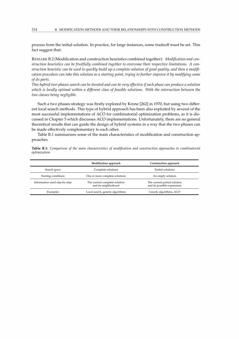
314 B. MODIFICATION METHODS AND THEIR RELATIONSHIPS WITH CONSTRUCTIONMETHODS
process from the initial solution. In practice, for large instances, some tradeoff must be set. This
fact suggest that:
REMARK B.2 (Modification and construction heuristics combined together): Modification and con-
struction heuristics can be fruitfully combined together to overcome their respective limitations. A con-
struction heuristic can be used to quickly build up a complete solution of good quality, and then a modifi-
cation procedure can take this solution as a starting point, trying to further improve it by modifying some
of its parts.
This hybrid two-phases search can be iterated and can be very effective if each phase can produce a solution
which is locally optimal within a different class of feasible solutions. With the intersection between the
two classes being negligible.
Such a two phases strategy was firstly explored by Krone [262] in 1970, but using two differ-
ent local search methods. This type of hybrid approach has been also exploited by several of the
most successful implementations of ACO for combinatorial optimization problems, as it is dis-
cussed in Chapter 5 which discusses ACO implementations. Unfortunately, there are no general
theoretical results that can guide the design of hybrid systems in a way that the two phases can
be made effectively complementary to each other.
Table B.1 summarizes some of the main characteristics of modification and construction ap-
proaches.
Table B.1: Comparison of the main characteristics of modification and construction approaches to combinatorialoptimization
Modification approach Construction approach
Search space Complete solutions Partial solutions
Starting conditions One or more complete solutions An empty solution
Information used step-by-step The current complete solution The current partial solutionand its neighborhood and its possible expansions
Examples Local search, genetic algorithms Greedy algorithms, ACO
APPENDIX C
Observable and partially observable
Markov decision processes
C.1 Markov decision processes (MDP)
Here we discuss some general characteristics of MDPs which have not been covered by the
brief introduction to MDP give in Subsection 3.3.4 (for a comprehensive treatment of the subject
see [353, 23]).
A decision (control) problem within the MDP framework consists in the search for an action
or a sequence of control actions for one or more states that optimizes some cost criterion J ,
starting from one or more initial states. The mapping of states into control actions is called the
decision policy, here indicated with π. The whole dynamics of the process is described by the
following state equation:
xt+1 = F (xt, uπt ), xt, xt+1 ∈ X, uπt ∈ U(xt), (C.1)
where it is assumed that the function F of the state evolution is known, as well as the starting
state x0. Each single control action is determined by the current action policy, and, accordingly, is
indicated as uπt . The purpose of the agent is to compute, or learn, the policy optimal with respect
to the criterion J . Therefore, the action policy might change during the process execution time.
The criterion to optimize is such that the costs incurred over time are combined into a single
quantity using various types of models. The cost criterion assesses the quality of the policies
followed by the agent in terms of total expected cost incurred by starting from a state x and
following the current policy π over a defined horizon H . Typically, the criterion to optimize is
an additive combination of the costs and, according to the probabilistic nature of the process, is
based on expectations:
J(x) = E
[
H∑
t=0
gt(
C(xt+1| xt, uπt ))
∣
∣
∣x0 = x
]
, (C.2)
where x is the starting state, and gt is a generic function to weight the contribution of each sin-
gle cost. The subscript t indicates that costs incurred at different time steps can be weighted in
different way. The horizon H can be finite or infinite [23]. In general, the use of an infinite hori-
zon allows a more sophisticated and insightful mathematical treatment, even if it is a condition
which is never satisfied in practice. Due to its mathematical appealing, infinite horizon model-
ing is also used to treat cases which naturally have a finite horizon, like shortest path problems
on direct acyclic graphs. In general, the finite horizon problems can be treated as a sub-class
of the infinite horizon ones once terminal, or absorbing, states are made recurrent with null-cost
self-transitions. In general, this approach is always feasible but requires some care when, for
example, average cost criteria are used to assess the quality of a policy (see below).
When the horizon is infinite, the sum J can be unbounded if no absorbing states are en-
countered. Therefore, a finite or bounded long-term measure of the quality of a policy must be
316 C. OBSERVABLE AND PARTIALLY OBSERVABLE MARKOV DECISION PROCESSES
defined. In these cases, a time-dependent cost discount factor γ ∈ [0, 1) is used and J takes the
following form:
gt = γtC(xt+1| xt, uπt )
J(x) = limH→∞
E
[
H∑
t=0
γtC(xt+1| xt, uπt )∣
∣
∣x0 = x
]
. (C.3)
In some cases, like in some economic-like domains where future costs matter less than the
cost incurred in earlier stages, discounting has its own rationale. In many other cases it is just a
useful mathematical tool. When there are no reasons to weight in a decreasing way the incurring
costs, an average costmeasure of optimality is used, to optimize the average cost per action:
gt =1
HC(xt+1| xt, uπt )
J(x) = limH→∞
1
HE
[
H∑
t=0
C(xt+1| xt, uπt )∣
∣
∣x0 = x
]
. (C.4)
For cyclic tasks this is maybe a better measure than the discounted one (see [287] for an insightful
discussion on discounting, averaging, and related measures of optimality).
If the horizon is finite and sums are bounded, then there is no mathematical need for aver-
aging and/or discounting. Expectations over the total costs incurred can be used, if the charac-
teristics of the problem do not suggest otherwise. In this case:
gt = C(xt+1| xt, uπt ),
J(x) = E
[
H∑
t=0
C(xt+1| xt, uπt )∣
∣
∣x0 = x
]
. (C.5)
Total costs can be in principle safely used for the class of finite combinatorial problems consid-
ered in this thesis. More in general, total costs can be properly used in the case of (stochastic)
shortest path problems over acyclic graphs. Using total costs in an online process can have some
drawbacks when the current (finite) length of the horizon is not known with precision.
For what concerns the computational complexity of MDPs, any discounted MDP can be repre-
sented as a linear program and solved in time polynomial in the size of the state space, action
space, and bits of precision required to encode instantaneous costs and state-transition probabil-
ities as rational numbers [279]. However, the order of the polynomials is large enough that the
theoretically efficient algorithms are not efficient in practice. Among the algorithms specific for
solving MDPs, none is known to run in worst-case polynomial time. The best known practical
algorithms for solving MDPs appear to be dependent on the discount rate γ for the number of
required iterations, which grows as
1
(1− γ) log(1/(1− γ)) . (C.6)
As γ → 1, that is, extending the effective horizon, the number of iterations grows indefinitely.
More in general, the properties of the state structure associated to the generated Markov chains,
like the mixing conditions [235], which are related to degree of conditional dependence among
the states, seem to suggest a more effective way to classify MDPs into easy and hard problems.
C.2 Partially observable Markov decision processes (POMDP)
The Markov decision process framework models a controlled stochastic process whose state are
assumed to be perfectly observable by the acting agent. There might be uncertainty about the
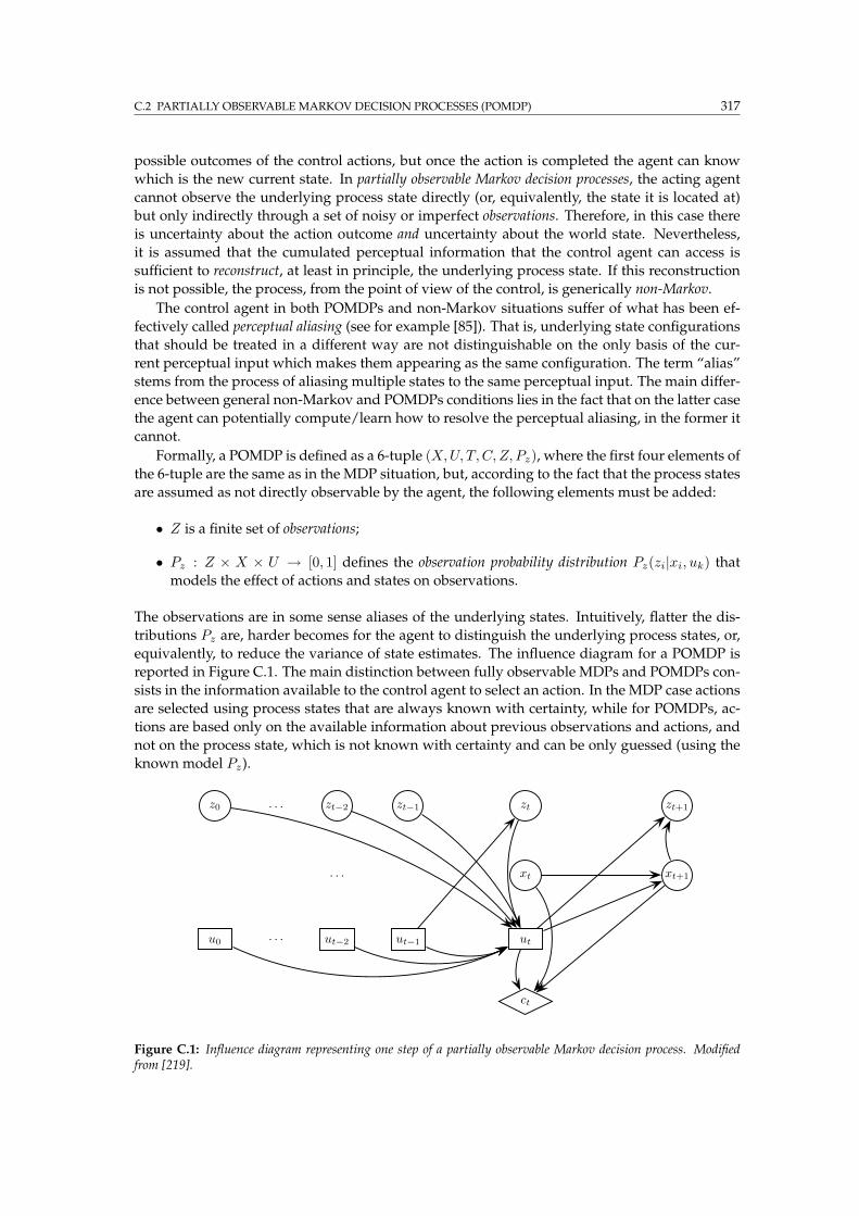
C.2 PARTIALLY OBSERVABLE MARKOV DECISION PROCESSES (POMDP) 317
possible outcomes of the control actions, but once the action is completed the agent can know
which is the new current state. In partially observable Markov decision processes, the acting agent
cannot observe the underlying process state directly (or, equivalently, the state it is located at)
but only indirectly through a set of noisy or imperfect observations. Therefore, in this case there
is uncertainty about the action outcome and uncertainty about the world state. Nevertheless,
it is assumed that the cumulated perceptual information that the control agent can access is
sufficient to reconstruct, at least in principle, the underlying process state. If this reconstruction
is not possible, the process, from the point of view of the control, is generically non-Markov.
The control agent in both POMDPs and non-Markov situations suffer of what has been ef-
fectively called perceptual aliasing (see for example [85]). That is, underlying state configurations
that should be treated in a different way are not distinguishable on the only basis of the cur-
rent perceptual input which makes them appearing as the same configuration. The term “alias”
stems from the process of aliasing multiple states to the same perceptual input. The main differ-
ence between general non-Markov and POMDPs conditions lies in the fact that on the latter case
the agent can potentially compute/learn how to resolve the perceptual aliasing, in the former it
cannot.
Formally, a POMDP is defined as a 6-tuple (X,U, T,C, Z, Pz), where the first four elements of
the 6-tuple are the same as in the MDP situation, but, according to the fact that the process states
are assumed as not directly observable by the agent, the following elements must be added:
• Z is a finite set of observations;
• Pz : Z × X × U → [0, 1] defines the observation probability distribution Pz(zi|xi, uk) that
models the effect of actions and states on observations.
The observations are in some sense aliases of the underlying states. Intuitively, flatter the dis-
tributions Pz are, harder becomes for the agent to distinguish the underlying process states, or,
equivalently, to reduce the variance of state estimates. The influence diagram for a POMDP is
reported in Figure C.1. The main distinction between fully observable MDPs and POMDPs con-
sists in the information available to the control agent to select an action. In the MDP case actions
are selected using process states that are always known with certainty, while for POMDPs, ac-
tions are based only on the available information about previous observations and actions, and
not on the process state, which is not known with certainty and can be only guessed (using the
known model Pz).
z0 · · · zt−2 zt−1 zt zt+1
· · · xt xt+1
u0 · · · ut−2 ut−1 ut
ct
Figure C.1: Influence diagram representing one step of a partially observable Markov decision process. Modifiedfrom [219].
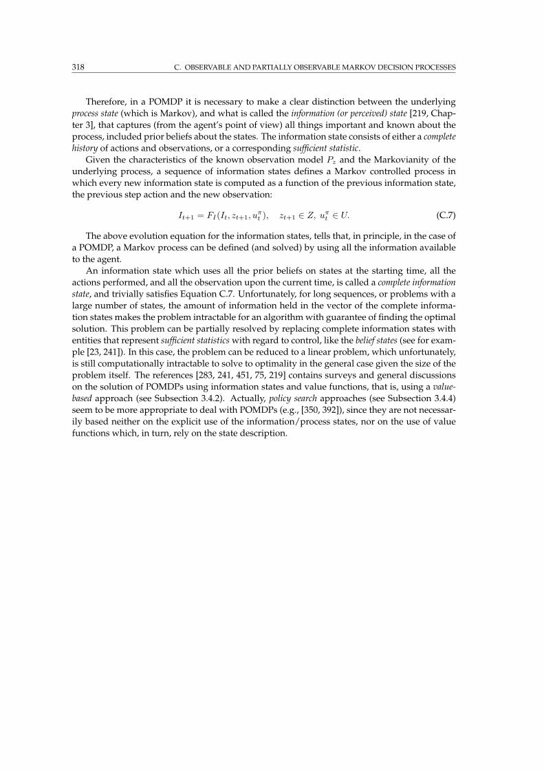
318 C. OBSERVABLE AND PARTIALLY OBSERVABLE MARKOV DECISION PROCESSES
Therefore, in a POMDP it is necessary to make a clear distinction between the underlying
process state (which is Markov), and what is called the information (or perceived) state [219, Chap-
ter 3], that captures (from the agent’s point of view) all things important and known about the
process, included prior beliefs about the states. The information state consists of either a complete
history of actions and observations, or a corresponding sufficient statistic.
Given the characteristics of the known observation model Pz and the Markovianity of the
underlying process, a sequence of information states defines a Markov controlled process in
which every new information state is computed as a function of the previous information state,
the previous step action and the new observation:
It+1 = FI(It, zt+1, uπt ), zt+1 ∈ Z, uπt ∈ U. (C.7)
The above evolution equation for the information states, tells that, in principle, in the case of
a POMDP, a Markov process can be defined (and solved) by using all the information available
to the agent.
An information state which uses all the prior beliefs on states at the starting time, all the
actions performed, and all the observation upon the current time, is called a complete information
state, and trivially satisfies Equation C.7. Unfortunately, for long sequences, or problems with a
large number of states, the amount of information held in the vector of the complete informa-
tion states makes the problem intractable for an algorithmwith guarantee of finding the optimal
solution. This problem can be partially resolved by replacing complete information states with
entities that represent sufficient statisticswith regard to control, like the belief states (see for exam-
ple [23, 241]). In this case, the problem can be reduced to a linear problem, which unfortunately,
is still computationally intractable to solve to optimality in the general case given the size of the
problem itself. The references [283, 241, 451, 75, 219] contains surveys and general discussions
on the solution of POMDPs using information states and value functions, that is, using a value-
based approach (see Subsection 3.4.2). Actually, policy search approaches (see Subsection 3.4.4)
seem to be more appropriate to deal with POMDPs (e.g., [350, 392]), since they are not necessar-
ily based neither on the explicit use of the information/process states, nor on the use of value
functions which, in turn, rely on the state description.
APPENDIX D
Monte Carlo statistical methods
Any generic method for carrying out variable estimations by means of operations involving a
significant random component is termed a Monte Carlo method [374, 367]. If the estimations are
carried out using a whatever approximate model of the system under study, the estimations are
said to be based on the outcomes of aMonte Carlo simulation process.
The vast framework of Monte Carlo statistical methods provides the theoretical basis and
the practical tools for a number of research domains of fundamental importance, like all those
domains related to the study of stochastic processes.
The general aim of Monte Carlo methods consist in solving one or both of the following
problems:
1. Generate samples from a given given distribution P (x);
2. Estimate expectation of functions under this distribution, like, for instance:
〈φ〉 =
∫
φ(x)P(x)dx. (D.1)
Clearly, to solve the second problem is necessary to solve the first in order to use the samples
to carry out the desired expectation estimate. Unfortunately, it is often not easy to sample from
a desired distribution, in particular from a high-dimensional one. Therefore, a number of tech-
niques have been devised in order to efficiently obtain representative samples and unbiased and
low variance estimates (e.g., [367, 374]).
The history of Monte Carlo methods is long and finds its roots in the the 1777 Buffon’s
work [198] on using needle throws to compute an approximation to π. The term “Monte Carlo”
was introduced by Von Neumann and Ulam during World War II as a code word for their se-
cret work at Los Alamos on neutron diffusion and adsorption. The use of the term was related
to the fact that they were heavily using stochastic simulation, and the Monte Carlo’s roulettes
represented one the simplest models for the generation of random variables.
In addition to the rather general characteristics given in the definition above, and which
are widely accepted in scientific community, in the specific community of reinforcement learn-
ing, Monte Carlo methods have been connoted more in specific as those statistical methods
which shares no similarities with the dynamic programming way of building up statistical esti-
mates [414]. That is, Monte Carlo methods for evaluation and control refer to statistical methods
for learning from the experience without using any form of information bootstrapping. A sim-
ple example can help to clarify this point of view. Let us imagine that, in order to estimate state
values (see Subsection 3.4.2), an experience h is generated by an agent and the sequence of states
(x1, x2, . . . , xn) is visited. Let us assume that an additive cost criterion is used to score the actions
of the agent and that Jh is the total accumulated cost at the end of the experience. The state-value
estimates V (x) can be updated on the basis of the costs-to-go that have been observed for the
states xi ∈ h visited during the experience h:
v(xi) =n−1∑
k=i
J (xk+1|xk), ∀xi ∈ h, xn terminal state. (D.2)
320 D. MONTE CARLO STATISTICAL METHODS
The critical point lies exactly in the way the V (x) are updated using the v(xi) resulting from the
experience. In the sense Monte Carlo is intended in reinforcement learning, every V (x),∀x ∈ his updated using the corresponding v(x) such that the resulting V (x) is some average of all the
v(x) incurred during all the generated experiences h. No bootstrapping (see Remark 3.18) is
actually performed in order to improve or speedup the computation of the estimates. In a sense,
every state is treated as independent, while, when a bootstrapping approach is used like in dy-
namic programming, estimates are propagated among the states, and the correlation structure
of the underlying Markov chain is fully exploited to obtain unbiased and low variance estimates
as quick as possible. The Bellman’s relationships between the states are the most basic relation-
ships existing between the states points, but they are better than nothing, and they are always
valid in spite of the specific characteristics of the problem at hand. Therefore, whenMonte Carlo
updating is used, a slower convergence is expectedwith respect to a bootstrapping-based updat-
ing strategy, since the Monte Carlo strategy will only make use of the information coming from
the experience, neglecting that related to the state structure. On the other hand, it must be clear
that a really effective use of the state structure in terms of information bootstrapping, would re-
quire the knowledge of the precise topology of the state set, which would serve to define where
the estimates should propagate according to the fact that two states are topologically close or
not. In typical reinforcement learning tasks, state information is rarely assumed to be known,
and it must be learned by direct interaction with the environment. Therefore, in these cases it
is not clear how to rank a priori the expected relative performance of Monte Carlo learning vs.
bootstrapping-based learning (e.g., see also [414, Chapters 5-6]).
Monte Carlo methods intended as statistical methods for learning (building estimates) from
the experience without using any form of information bootstrapping appears suitable to be used
in the case of POMDPs, or generic non-Markov representations when the states are not directly
accessible. That is, in those cases inwhich assuming some form of correlation among entities that
are not states can result in completely wrong estimates. On the other side, when the underlying
problem at hand is an MDP, the Monte Carlo and dynamic programming approaches can be
fruitfully combined, even if the environment’s model is fully available. This is actually what
is effectively done in the important class of reinforcement learning algorithms called temporal
differences [413, 391, 414].
Throughout the thesis, the activities of performing sampling experiments on the problem
environment or on a model of it are referred to as Monte Carlo. More in general, when not
explicitly stated, the term Monte Carlo is used with the same specialized meaning it is used in
the field of reinforcement learning.
APPENDIX E
Reinforcement learning
When the model of the environment is available, that is, when the dynamics for state transition
and cost generation are perfectly known, the problem at hand can be in principle solved to
optimality by solving the Bellman’s equations 3.36. The equations can be solved in numerical or
analytical way, according to themathematical properties of the involved functions. The situation
is rather different when the model is not available. Clearly, in this case is impossible to solve
directly the equations because it is impossible to precisely write them down. The optimization
agent is therefore forced to acquire the missing information by possibly interacting directly with
the environment. That is, direct or simulated experience must be acquired in order to estimate the
variables of interest. Experience can be used to build up the missing model, that can be in turn
used to solve the equations. For the problems of interest this approach is often not an efficient
one. The effort necessary to build up a trusting model can be focusedmore conveniently to build
up directly the statistical estimates of the variables of interest. That is, the value of the states, or,
in the case of policy search, the value of the policy itself.
The research domain which is specifically addressed to the study of decision problems in ab-
sence of a perfect model of the environment is that of reinforcement learning. Generally speaking,
reinforcement learning refers to learning from direct interaction with an environment in absence
of a perfect model of the environment and of a training set of labeled examples (which is the case
of so-called supervised learning). The learning agent can receive just a reinforcement/advisory
signal from the environment, and not a precise error signal measuring the discrepancy between
the realized and a known expected performance. Learning a decision policy without a labeled
training set and a model of the environment determines the need for: (i) a direct interaction with
the environment, (ii) the exploitation of any kind of advisory signal the environment can pro-
vide regarding the executed actions, (iii) the use of an exploratory component while interacting
with the environment in order to explore the environment itself to discover the best actions in
relationship to the environment states.
Every sequential decision task which is not supervised and which need to be solved by
means of information collected by direct interaction with the environment for the inability to
directly solve model equations, can be framed as a reinforcement learning problem. In addition
to this class of problems also the general delayed rewards problems, that is, problems in which
only sporadic signals are received from the environment, are usually classified as reinforcement
learning problems. In fact, in these cases dynamic programming cannot perform efficiently even
if the model of the environment is available, and is therefore is necessary to use different tech-
niques. Usually, delayed rewards come from real-world problems, like foraging, that require a
direct interaction with the environment.
Generally speaking, reinforcement learning refers to a class of problems rather than to a class
of techniques.
The literature on reinforcement learning is extensive. The references [414, 27, 350, 219] offer
a comprehensive, insightful and somehow complementary introduction to the field, covering
most of the major issues considered so far.

APPENDIX F
Classification of telecommunication
networks
A network is a set of nodes that are interconnected through links to permit the exchange of in-
formation. Data traffic originates from one node and can be directed to another node (unicast
traffic), to a set of other nodes (multicast traffic) and/or to all the other nodes (broadcast traffic).
Nodes can be connected by means of either wired cables or radio interfaces, and their relative
position can be dynamically changing (mobile networks) or be static in practice. User nodes can
communicate through the use of infrastructures (in the form of specialized gateways/routers), or
they can act themselves as routers to form an ad hoc, infrastructureless, network.
Classifications over the existing networks can be done according to a number of different
criteria, ranging from physical characteristics for transmission and connectivity, to strategies for
the utilization of the transmission technology, to the organization at the nodes of the activities of
data processing and forwarding. Some among the most important criteria are briefly considered
in the following subsections, where each subsection focuses on one single criterion. According
to the fact that in this thesis most of the focus is on wired data networks, most of the discussion
will precisely concern these types of networks.
F.1 Transmission technology
The most immediate distinction in terms of transmission technology is between wired and wire-
less networks. That is, networks making use of cabled links versus networks making use of
radio links. The range of network utilization being greatly affected by the specific physical char-
acteristics of the network links whose bandwidth can range from the few kilobits/sec of a cheap
parallel or serial cable, to the several Gbits/sec of all-optical links.
In more general sense, there are two types of transmission technology to interconnect the
nodes: broadcast links and point-to-point links.
Broadcast links have a single communication channel that is shared by all the nodes on the
network. Messages sent by any node are received by all the others sharing the same channel. An
address field within the packet can be used to specify the intended recipient. After receiving a
packet, a node can check the address field. If the packet is intended for itself the node processes
the packet, if not, it is just ignored. Ethernet networks are precisely based on the use of broadcast
links. Point-to-point networks consist of single connections between individual pairs of nodes.
As a general rule for the case of wired networks, smaller geographically localized networks
tend to use broadcasting technology, whereas larger networks usually are point-to-point. Wire-
less networks are an in-between-case since the channel is in principle shared by all the nodes
but limitations in the signal power do make it rarely possible a real broadcast communication.
In this case it can be said that the link is of multicast type since the signal is broadcast in practice
only to a subset (those in the physical reception range) of all the network nodes.
324 F. CLASSIFICATION OF TELECOMMUNICATION NETWORKS
In the case of broadcast links, a critical issue consists in the channel contention access among
the nodes, due to the fact that the channel is a shared resource. This issue becomes of par-
ticular relevance for the case of mobile wireless networks. For GSM networks the problem is
in a sense solved by the base stations placed on the ground, which provide to assign different
communication frequencies to the mobile nodes, such that the single radio channel becomes in
practice equivalent to n different frequency channels that can be used concurrently (e.g., see also
the discussions on the frequency assignment problem at Page 155). On the other hand, in the
case of mobile ad hoc networks, which are mobile wireless networks lacking of an infrastructure
in the sense of not relying on antennas / base stations, the radio channel is really a fully shared
resource, and contention problems are a major drawback (that, added to the fact that network
topology is continually changing because of node mobility and nodes switching on and off,
makes this type of networks quite hard to deal with in an effective way).
F.2 Switching techniques
Three main switching techniques have been proposed to effectively share the available transmis-
sion links among multiple users (the end systems) located at the nodes (the intermediate systems):
Circuit-switching: It is used for ordinary telephone networks and is characterized by the fact
that network resources are reserved all the way from sender to receiver before the start of
the transfer, thereby creating a circuit. The resources are dedicated to the circuit during
the whole transfer. Control signaling and payload data transfers are separated. Processing
of control information and control signaling such as routing is performed mainly at circuit
setup and termination. Consequently, the transfer of payload data within the circuit does
not contain any overhead in the form of headers or the like. Electronic interfaces in the
switches convert the analog signal into the digital one, called a bit stream, and vice versa.
An advantage of circuit-switched networks is that they allow for large amounts of data to
be transferred with guaranteed transmission capacity, thus providing support for real-time
traffic. A disadvantage of circuit switching, however, is that if connections are short-lived
when transferring short messages, for example the setup delay may represent a large part
of the total connection time, thus reducing the network’s capacity. Moreover, reserved
resources cannot be used by any other users even if the circuit is inactive, which may
further reduce link utilization.
Packet-switching: It is used in computer networks exchanging data in the form of packets of
bits. In packet switching, a data stream is divided into standardized packets. Each packet
contains address, size, sequence, and error-checking information, in addition to the pay-
load data. Once packets are sent into the network, specific packet switches or routers sort
and direct them one-by-one. Packet-switched networks were developed to cope more ef-
fectively with the data-transmission limitations of the circuit-switched networks during
bursts of random traffic, in order to obtain a more efficient exploitation of the available
network resources.
Packet-switched networks are based either on connection-less (datagram) or connection-oriented
(virtual-circuit) strategies for packet forwarding. These two complementary strategies are
discussed in depth the following.
Asynchronous transfer mode (ATM): This uses a connection-oriented approach, setting up a
connection, and multiplexing and switching fixed size cells onto the the connection. The
connection has reduced functionality from the traditional circuit-switched type connec-
tion and is made possible by making assumptions about the reliability and capacity of the
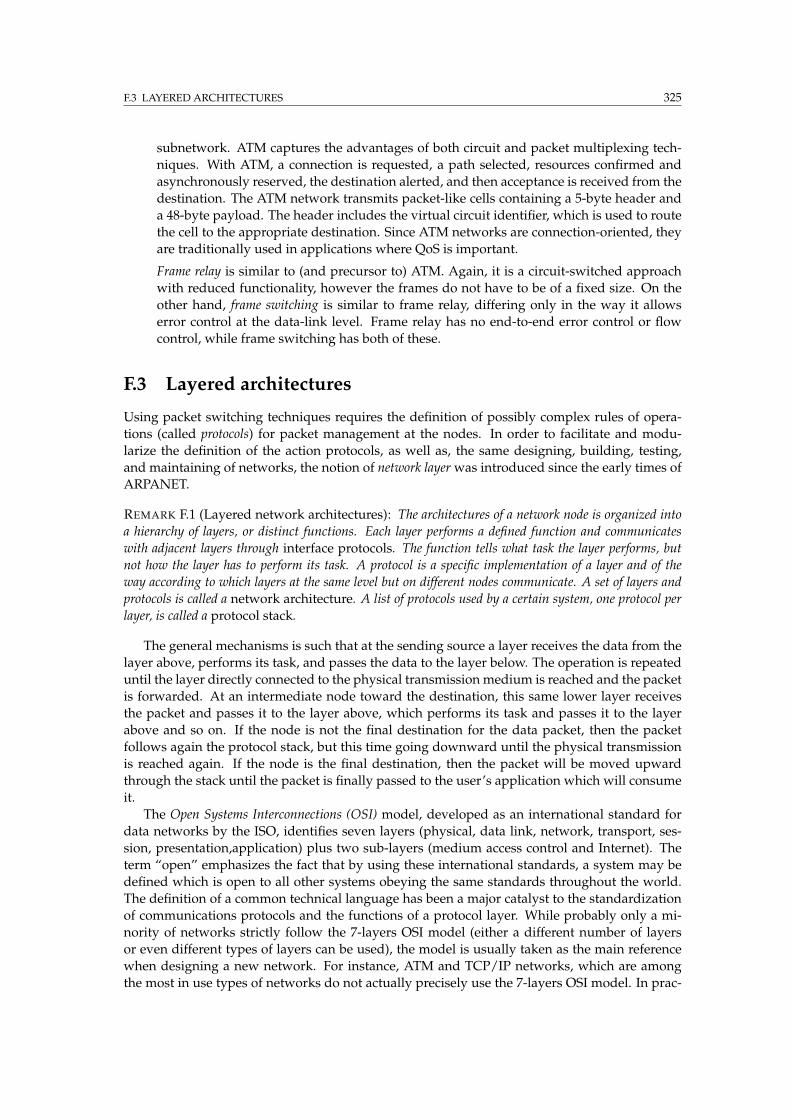
F.3 LAYERED ARCHITECTURES 325
subnetwork. ATM captures the advantages of both circuit and packet multiplexing tech-
niques. With ATM, a connection is requested, a path selected, resources confirmed and
asynchronously reserved, the destination alerted, and then acceptance is received from the
destination. The ATM network transmits packet-like cells containing a 5-byte header and
a 48-byte payload. The header includes the virtual circuit identifier, which is used to route
the cell to the appropriate destination. Since ATM networks are connection-oriented, they
are traditionally used in applications where QoS is important.
Frame relay is similar to (and precursor to) ATM. Again, it is a circuit-switched approach
with reduced functionality, however the frames do not have to be of a fixed size. On the
other hand, frame switching is similar to frame relay, differing only in the way it allows
error control at the data-link level. Frame relay has no end-to-end error control or flow
control, while frame switching has both of these.
F.3 Layered architectures
Using packet switching techniques requires the definition of possibly complex rules of opera-
tions (called protocols) for packet management at the nodes. In order to facilitate and modu-
larize the definition of the action protocols, as well as, the same designing, building, testing,
and maintaining of networks, the notion of network layerwas introduced since the early times of
ARPANET.
REMARK F.1 (Layered network architectures): The architectures of a network node is organized into
a hierarchy of layers, or distinct functions. Each layer performs a defined function and communicates
with adjacent layers through interface protocols. The function tells what task the layer performs, but
not how the layer has to perform its task. A protocol is a specific implementation of a layer and of the
way according to which layers at the same level but on different nodes communicate. A set of layers and
protocols is called a network architecture. A list of protocols used by a certain system, one protocol per
layer, is called a protocol stack.
The general mechanisms is such that at the sending source a layer receives the data from the
layer above, performs its task, and passes the data to the layer below. The operation is repeated
until the layer directly connected to the physical transmission medium is reached and the packet
is forwarded. At an intermediate node toward the destination, this same lower layer receives
the packet and passes it to the layer above, which performs its task and passes it to the layer
above and so on. If the node is not the final destination for the data packet, then the packet
follows again the protocol stack, but this time going downward until the physical transmission
is reached again. If the node is the final destination, then the packet will be moved upward
through the stack until the packet is finally passed to the user’s application which will consume
it.
The Open Systems Interconnections (OSI) model, developed as an international standard for
data networks by the ISO, identifies seven layers (physical, data link, network, transport, ses-
sion, presentation,application) plus two sub-layers (medium access control and Internet). The
term “open” emphasizes the fact that by using these international standards, a system may be
defined which is open to all other systems obeying the same standards throughout the world.
The definition of a common technical language has been a major catalyst to the standardization
of communications protocols and the functions of a protocol layer. While probably only a mi-
nority of networks strictly follow the 7-layers OSI model (either a different number of layers
or even different types of layers can be used), the model is usually taken as the main reference
when designing a new network. For instance, ATM and TCP/IP networks, which are among
the most in use types of networks do not actually precisely use the 7-layers OSI model. In prac-
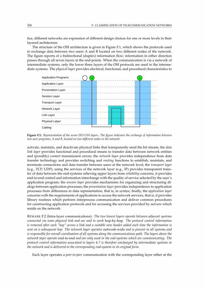
326 F. CLASSIFICATION OF TELECOMMUNICATION NETWORKS
tice, different networks are expression of different design choices for one or more levels in their
layered architecture.
The structure of the OSI architecture is given in Figure F.1, which shows the protocols used
to exchange data between two users A and B located on two different nodes of the network.
The figure reports of a bidirectional (duplex) information flow; information in either direction
passes through all seven layers at the end-points. When the communication is via a network of
intermediate systems, only the lower three layers of the OSI protocols are used in the interme-
diate systems. The physical layer provides electrical, functional, and procedural characteristics to
Physical Lalyer
Link Layer
Network Layer
Transport Layer
Session Layer
Presentation Layer
Application Layer
Application Programs
Cabling
BA
Figure F.1: Representation of the seven ISO-OSI layers. The figure indicates the exchange of information betweentwo user programs, A and B, located on two different nodes in the network.
activate, maintain, and deactivate physical links that transparently send the bit stream; the data
link layer provides functional and procedural means to transfer data between network entities
and (possibly) correct transmission errors; the network layer provides independence from data
transfer technology and provides switching and routing functions to establish, maintain, and
terminate connections and data transfer between users at the network level; the transport layer
(e.g., TCP, UDP), using the services of the network layer (e.g., IP) provides transparent trans-
fer of data between the end-systems relieving upper layers from reliability concerns, it provides
end-to-end control and information interchange with the quality of service selected by the user’s
application program; the session layer provides mechanisms for organizing and structuring di-
alogs between application processes; the presentation layer provides independence to application
processes from differences in data representation, that is, in syntax; finally, the application layer
concerns with the requirements of applications to access the network services, that is, it provides
library routines which perform interprocess communication and deliver common procedures
for constructing application protocols and for accessing the services provided by servers which
reside on the network.
REMARK F.2 (Intra-layer communications): The two lowest layers operate between adjacent systems
connected via some physical link and are said to work hop-by-hop. The protocol control information
is removed after each ”hop” across a link and a suitable new header added each time the information is
sent on a subsequent hop. The network layer operates network-wide and is present in all systems and
is responsible for overall coordination of all systems along the communications path. The layers above the
network layer operate end-to-end and are only used in the end-systems which are communicating. The
protocol control information associated to layers 4-7 is therefore unchanged by intermediate systems in
the network and is delivered to the corresponding end-system in its original form.
Each layer operates a peer-to-peer communication with the corresponding layer either at the
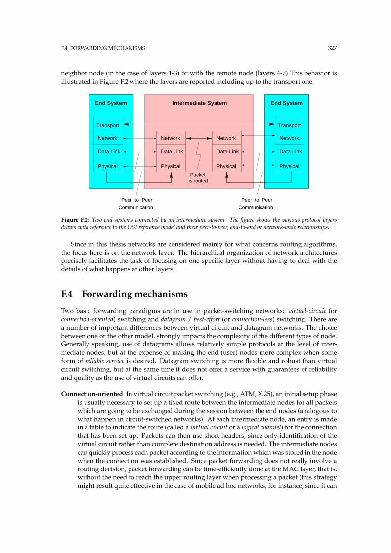
F.4 FORWARDINGMECHANISMS 327
neighbor node (in the case of layers 1-3) or with the remote node (layers 4-7) This behavior is
illustrated in Figure F.2 where the layers are reported including up to the transport one.
Transport
Network
Data Link
Physical
Transport
Network
Data Link
Physical
End System
Network
Data Link
Physical
Network
Data Link
Physical
Intermediate System End System
Communication
Peer−to−Peer
Communication
Packet
Peer−to−Peer
is routed
Figure F.2: Two end-systems connected by an intermediate system. The figure shows the various protocol layersdrawn with reference to the OSI reference model and their peer-to-peer, end-to-end or network-wide relationships.
Since in this thesis networks are considered mainly for what concerns routing algorithms,
the focus here is on the network layer. The hierarchical organization of network architectures
precisely facilitates the task of focusing on one specific layer without having to deal with the
details of what happens at other layers.
F.4 Forwarding mechanisms
Two basic forwarding paradigms are in use in packet-switching networks: virtual-circuit (or
connection-oriented) switching and datagram / best-effort (or connection-less) switching. There are
a number of important differences between virtual circuit and datagram networks. The choice
between one or the other model, strongly impacts the complexity of the different types of node.
Generally speaking, use of datagrams allows relatively simple protocols at the level of inter-
mediate nodes, but at the expense of making the end (user) nodes more complex when some
form of reliable service is desired. Datagram switching is more flexible and robust than virtual
circuit switching, but at the same time it does not offer a service with guarantees of reliability
and quality as the use of virtual circuits can offer.
Connection-oriented In virtual circuit packet switching (e.g., ATM, X.25), an initial setup phase
is usually necessary to set up a fixed route between the intermediate nodes for all packets
which are going to be exchanged during the session between the end nodes (analogous to
what happen in circuit-switched networks). At each intermediate node, an entry is made
in a table to indicate the route (called a virtual circuit or a logical channel) for the connection
that has been set up. Packets can then use short headers, since only identification of the
virtual circuit rather than complete destination address is needed. The intermediate nodes
can quickly process each packet according to the information which was stored in the node
when the connection was established. Since packet forwarding does not really involve a
routing decision, packet forwarding can be time-efficiently done at the MAC layer, that is,
without the need to reach the upper routing layer when processing a packet (this strategy
might result quite effective in the case of mobile ad hoc networks, for instance, since it can
328 F. CLASSIFICATION OF TELECOMMUNICATION NETWORKS
allow to make an optimized use of all the handshaking signals that are necessary to be
exchanged for a reliable communication can happen [4].
Since a node is required to keep state information about all sessions whose circuits pass
through it, a disconnect phase at the end of data transfer is required (as in the circuit-
switched network) in order to clear up memory resources.
As an alternative to keep session state information, source routing can be used to emulate
virtual circuits: at the source node each data packet is created together with a complete
specification of the node path that it has to follow. In this way routers are not required to
keep state information about sessions’ circuits, packets do.
The use of virtual circuits gives the possibility of offering a reliable service directly at the
network layer: delivery of packets in proper sequence and with essentially no errors can
be guaranteed, and congestion control to minimize queuing is common. By physically re-
serving the resources on the nodes, a virtual circuit network can also provide guaranteed
quality-of-service in terms of end-to-end delay or other metrics. Without resources reserva-
tion, each circuit may compete with the others for the same resources. In this case delays
might be more variable but they are usually more stable than in the datagram case. In
general, the use of virtual circuits compared to the use of datagrams allows for a more di-
rect control on the dynamics of packet routing and, consequently, allows for a service more
reliable and with some level of guaranteed quality.
Connection-less In the connection-less approach, there is no need of setup phases or session
state information maintained at the routing nodes. Each data packet is treated as an inde-
pendent entity. Each packet contains a header with the full information about the intended
recipient. The intermediate nodes examine the header of the packet and on the basis of a
per-packet decision it selects an appropriate link to an intermediate node which is nearer
(in some sense) to the destination. Accordingly, data packets from a same session can pos-
sibly follow different paths and the intermediate nodes do not require prior knowledge of
the routes that will be used.
In a datagram network delivery is not guaranteed (although they are usually reliably sent),
as well as a correct packet ordering. The service is said of type best-effort. Enhancements,
if required, to the basic service (e.g., reliable delivery and packet reordering) must be pro-
vided by the end systems using additional components. The most common datagram net-
work is the Internetwhich uses the IP network protocol. Applications which do not require
more than a best-effort service can be supported by direct use of packets in a datagram
network, using the User Datagram Protocol (UDP) transport protocol. Such applications
include Internet video, voice communications, e-mail notification, etc. However, most In-
ternet applications need additional functions to provide reliable communication (such as
end-to-end error and sequence control). Examples include sending e-mail, web browsing,
or file sending using the file transfer protocol (ftp). In these cases reliability is provided by
additional layers of software algorithms implemented in the end systems, that is, likely at
the transport layer by the Transmission Control Protocol (TCP).
One merit of the datagram approach is that not all packets need to follow the same route
through the network (although frequently packets do follow the same route). This removes
the need to set-up and tear-down the path, reducing the processing overhead, and a need
for intermediate systems to execute an additional protocol. Packets may also be routed
around busy parts of the network when alternate paths exist. This is useful when a particu-
lar intermediate system becomes busy or overloaded with excessive volumes of packets to
send. It can also provide a high degree of fault tolerance, when an individual intermediate
system or communication interface fails. As long as a route exists through the network
F.5 DELIVERED SERVICES 329
between two end-systems, they can in principle able to communicate, depending on the
characteristics of adaptivity of the routing protocol.
F.5 Delivered services
Networks and network layers can be classified according to the nature of their delivered services.
The following three major classes of services are usually considered.
Best-effort: Networks like most parts of the current Internet are said providing a best-effort ser-
vice at the routing layer, in the sense that there is no guarantee on the quality of the de-
livered performance The system is just tries to provide the overall “best” service it can
provide, considering that no reservation or prioritization of resources is admitted, and
that there is no control on the resources used by each specific session. In this sense, the
provided service can be quite “unfair” and governed by factors completely out of the user
control. For example, according to the traffic load, the completion time of the FTP down-
loading of a same big file in different moments can present a big variability, and the user
has no way to “complain” or to impose constraints on the downloading time.
A best-effort service, not only does not provide any guarantee on the quality of the deliv-
ered performance, but also does not provide full reliability. Where reliable delivery means
that data is accepted at one end of a link in the same order as it was transmitted at the other
end, without loss andwithout duplicates. A best-effort service at the network layer usually
performs some error control (e.g. discarding all frames which may have been corrupted)
and may also provided some (limited) retransmission. However, a reliable delivering of
data is not guaranteed, requiring reliability to be provided by a higher layer protocol (e.g.,
the TCP in the case of the Internet).
Fair-share: In networks with virtual circuits or source routing, fair-share routing schemes can be
implemented [286]. In this case the protocol characteristics of the routing layer are such
that the network utilization tends to be equally distributed over all the active applications.
In these networks there is a “fair sharing” of the available resources which is made possible
by a more direct control over the path which are followed by the running data flows.
Again, the FTP downloading time of a same file can show important oscillations, but this
time the user knows that he/she is getting a quite fair fraction of the network resources.
Quality-of-Service: At the other extreme of best-effort networks there are networks providing
quality-of-service (QoS) (e.g., see [440] for a good overview). In this case, the application
(the user) explicitly specifies the resources it needs, for example in terms of bandwidth or
delay jitter, and the network, once it accepts the application, is in some sense committed to
deliver the required resources to the application.
The notion of QoS captures the fact that, qualitatively or quantitatively, user applications
and network (the service provider) can negotiate the delivery of a specific performance.
The required performance can be expressed by hard or soft constraints. In general, con-
straints can be put on links, on whole paths, or on sets of rooted paths, that is, on trees.
On each of these topological elements specific physical constraints can be defined. For
example, a bandwidth constraint requires that each link on the path must have a specified
amount of free bandwidth, a delay constraint puts a limit on the maximal end-to-end delay
associated to the whole path, or, on the longest end-to-end delay for all paths of an entire
multicast tree (see for example [79, 440, 208] for overviews on QoS routing).
Once received the details about the requirements of the user application, the networkmust:
(i) find the resources, and (ii) guarantee their availability for all the lifetime of the appli-
330 F. CLASSIFICATION OF TELECOMMUNICATION NETWORKS
cation. If the system cannot meet these two conditions it is forced to refuse the session,
incurring in a negative payoff. The management of the whole process (i-ii) is rather com-
plex, and involves not only the routing component but also the connection admission con-
trol (CAC) component. The CAC component makes of use of routing layer information
to check if there is any path connecting the application end-points that meets the QoS re-
quirements of the application. If one or more paths can be found, the CAC evaluates the
convenience (in terms of costs, benefits, forecasting of network status, etc.) of accepting
or not the application. In the positive case, one (or more than one) of the QoS-feasible
paths are selected to route the application, and the required resources are either reserved
on these paths (e.g., this is what happens in the case of the Integrated Services architecture
and of the MPLS protocol) or provisioned by a combination of limiting at the edge the total
amount of traffic that the user can inject and adjusting routing paths (this is the case of the
Differentiated Services architecture). With Integrated Services the required quality is guar-
anteed according to a per-flow reservation. On the other hand, with Differentiated Services
no resources are reserved, users’ traffic is divided into a small number of forwarding classes
and aggregated, and for each forwarding class the amount of traffic that the user can inject
is limited at the edge of the network. This fact, together with a proper management of the
resources inside the network and of the routing paths, as well as with a prioritization of
the forwarding classes, can still provide deterministic guarantee on the offered service.
In general, to provide and sustain QoS, the network management system must deal with
resource availability and allocation and control policies. The systemmust compute/estimate
the feasibility and convenience of allocating a new QoS application. At the same time, it
must ensure that the contracted QoS is sustained, monitoring the network status and possi-
bly reallocating resources in response to anomalies or heavily unbalanced situations. From
this picture it is quite clear that when QoS is involved, the network management becomes
much more complex than in the best-effort case. In particular, the metrics that are used to
score the whole network performance become much more complex and are made up by
several, often conflicting criteria.
Most the forthcoming data and (interactive) multimedia network applications will require
some form of hard or soft QoS, in terms, for example, of guaranteed end-to-end delay,
bandwidth, delay jitter, loss rate, etc. QoS technologies provide the tools to deliver mis-
sion critical business over the networks. This fact is opening a wide range of different
possibilities in network utilization and pricing. Actually this perspective has attracted the
interest of a large number of companies and governmental institutions, making the re-
search in the field of QoS very active. The range of proposed solutions is quite wide, also
because different types of networks (e.g., ATM, IP, wireless, frame relay) have different
characteristics at the different layers. In particular, QoS research is very active for ATM,
IP, and mobile networks for which international committees work to define specifications,
requirements and algorithms.

Bibliography
331

Bibliography
[1] E. Aarts and J. Korst. Simulated Annealing and Boltzmann Machines, A Stochastic Approach to Combina-
torial Optimization and Neural Computing. Wiley, 1989.
[2] E.H. Aarts and J. K. Lenstra, editors. Local Search in Combinatorial Optimization. John Wiley & Sons,
Chichester, UK, 1997.
[3] T. Abe, S. A. Levin, and M. Higashi, editors. Biodiversity: an ecological perspective. Springer-Verlag,
New York, USA, 1997.
[4] A. Acharya, A. Misra, and S. Bansal. A label-switching packet forwarding architecture for multi-hop
wireless LANs. In Proceedings of the 5th ACM international workshop onWireless mobile multimedia, 2002.
[5] C. Alaettinoglu, A. U. Shankar, K. Dussa-Zieger, and I. Matta. Design and implementation of MaRS:
A routing testbed. Technical Report UMIACS-TR-92-103, CS-TR-2964, Institute for Advanced Com-
puter Studies and Department of Computer Science, University of Maryland, College Park (MD),
August 1992.
[6] D.A. Alexandrov and Y.A. Kochetov. The behavior of the ant colony algorithm for the set cov-
ering problem. In K. Inderfurth, G. Schwodiauer, W. Domschke, F. Juhnke, P. Kleinschmidt, and
G. Wascher, editors, Operations Research Proceedings 1999, pages 255–260. Springer-Verlag, 2000.
[7] S. Appleby and S. Steward. Mobile software agents for control in telecommunications networks. BT
technology Journal, 12(2), 1994.
[8] A.F. Atlasis, M.P. Saltouros, and A.V. Vasilakos. On the use of a Stochastic Estimator Learning Algo-
rithm to the ATM routing problem: a methodology. Computer Communications, 21(538), 1998.
[9] D.O. Awduche, A. Chiu, A. Elwalid, I. Widjaja, and X.P. Xiao. A framework for Internet traffic
engineering. Internet Draft draft-ietf-tewg-framework-05, Internet Engineering Task Force - Traffic
Engineering Working Group, January 2000.
[10] T. R. Balch. Hierarchic social entropy: An information theoretic measure of robot group diversity.
Autonomous Robots, 8(3):209–238, 2000.
[11] S. Baluja and R. Caruana. Removing the genetics from the standard genetic algorithm. In A. Prieditis
and S. Russell, editors, Proceedings of the Twelfth International Conference on Machine Learning (ML-95),
pages 38–46. Palo Alto, CA: Morgan Kaufmann, 1995.
[12] S. Baluja and S. Davies. Fast probabilistic modeling for combinatorial optimization. In Proceedings of
AAAI-98, 1998.
[13] B. Baran and R. Sosa. A new approach for AntNet routing. In Proceedings of the 9th International
Conference on Computer Communications Networks, Las Vegas, USA, 2000.
[14] J.S. Baras and H. Mehta. A probabilistic emergent routing algorithm for mobile ad hoc networks. In
WiOpt03: Modeling and Optimization in Mobile, Ad Hoc and Wireless Networks, 2003.
[15] A. G. Barto, R. S. Sutton, and C. W. Anderson. Neuronlike adaptive elements that can solve difficult
learning control problems. IEEE Transaction on Systems, Man and Cybernetics, SMC-13:834–846, 1983.
[16] A.G. Barto, S.J. Bradtke, and S.P. Singh. Learning to act using real-time dynamic programming.
Artificial Intelligence, 72:81–138, 1995.
[17] A. Bauer, B. Bullnheimer, R. F. Hartl, and C. Strauss. An Ant Colony Optimization approach for the
single machine total tardiness problem. In Proceedings of the 1999 Congress on Evolutionary Computa-
tion, pages 1445–1450. IEEE Press, Piscataway, NJ, USA, 1999.
334 BIBLIOGRAPHY
[18] R. Beckers, J. L. Deneubourg, and S. Goss. Trails and U-turns in the selection of the shortest path by
the ant Lasius Niger. Journal of Theoretical Biology, 159:397–415, 1992.
[19] M. Beckmann, C.B. McGuire, and C.B. Winstein. Studies in the Economices of Transportation. Yale
University Press, 1956.
[20] R. Bellman. Dynamic Programming. Princeton University Press, 1957.
[21] R. Bellman. On a routing problem. Quarterly of Applied Mathematics, 16(1):87–90, 1958.
[22] H. Bersini, M. Dorigo, S. Langerman, G. Seront, and L. M. Gambardella. Results of the first interna-
tional contest on evolutionary optimisation (1st ICEO). In Proceedings of IEEE International Conference
on Evolutionary Computation, IEEE-EC 96, pages 611–615. IEEE Press, 1996.
[23] D. Bertsekas. Dynamic Programming and Optimal Control, volume I–II. Athena Scientific, 1995.
[24] D. Bertsekas. Network Optimization: Continuous and Discrete Models. Athena Scientific, 1998.
[25] D. Bertsekas and D. Castanon. Rollout algorithms for stochastic scheduling problems. Journal of
Heuristics, 5(1):89–108, 1999.
[26] D. Bertsekas and R. Gallager. Data Networks. Prentice–Hall, Englewood Cliffs, NJ, USA, 1992.
[27] D. Bertsekas and J. Tsitsiklis. Neuro-Dynamic Programming. Athena Scientific, 1996.
[28] D. Bertsekas, J. N. Tsitsiklis, and Cynara Wu. Rollout algorithms for combinatorial optimization.
Journal of Heuristics, 3(3):245–262, 1997.
[29] S. Besher and J.H. Fewell. Models of division of labor in social insects. Annual Review of Entomology,
46:413–440, 2001.
[30] L. Bianchi, L. M. Gambardella, and M. Dorigo. Solving the homogeneous probabilistic traveling
salesman problem by the ACO metaheuristic. In M. Dorigo, G. Di Caro, and M. Sampels, editors,
Ants Algorithms - Proceedings of ANTS 2002, Third International Workshop on Ant Algorithms, volume
2463 of Lecture Notes in Computer Science, pages 176–187. Springer-Verlag, 2002.
[31] L. Bianchi, L. M. Gambardella, and M. Dorigo. An ant colony optimization approach to the prob-
abilistic traveling salesman problem. In Proceedings of PPSN-VII, Seventh International Conference on
Parallel Problem Solving from Nature, volume 2439 of Lecture Notes in Computer Science. Springer Verlag,
Berlin, Germany, 2002.
[32] N. Biggs, E. Lloyd, and R. Wilson. Graph theory 1736-1936. Oxford University Press, 1976.
[33] M. Birattari, G. Di Caro, and M. Dorigo. For a formal foundation of the Ant Programming approach
to combinatorial optimization. Part 1: The problem, the representation, and the general solution strat-
egy. Technical Report TR-H-301, Advanced Telecommunications Research Institute (ATR), Human
Information Processing Laboratories, Kyoto, Japan, December 2000.
[34] M. Birattari, G. Di Caro, and M. Dorigo. Toward the formal foundation of ant programming. In
M. Dorigo, G. Di Caro, and M. Sampels, editors, Ants Algorithms - Proceedings of ANTS 2002, Third
International Workshop on Ant Algorithms, Brussels, Belgium, September 12–14, 2002, volume 2463 of
Lecture Notes in Computer Science, pages 188–201. Springer-Verlag, 2002.
[35] C. M. Bishop. Neural Networks for Pattern Recognition. Oxford University Press, 1995.
[36] J.A. Bland. Optimal structural design by Ant Colony Optimization. Engineering optimization, 33:
425–443, 2001.
[37] J.A. Bland. Layout of facilities using an Ant System approach. Engineering optimization, 32(1), 1999.
[38] J.A. Bland. Space-planning by Ant Colony Optimization. International Journal of Computer Applications
in Technology, 12, 1999.
[39] L. Blazevic, L. Buttyan, S. Capkun, S. Giordano, J.-P. Hubaux, and J.-Y. Le Boudec. Self-organization
in mobile ad-hoc networks: the approach of terminodes. IEEE Communications Magazine, 39(6), June
2001.
[40] L. Blazevic, S. Giordano, and J.-Y. Le Boudec. Self organized terminode routing. Journal of Cluster
Computing, April 2002.
BIBLIOGRAPHY 335
[41] C. Blum. Aco applied to group shop scheduling: a case study on intensification and diversification.
In M. Dorigo, G. Di Caro, and M. Sampels, editors, Ants Algorithms - Proceedings of ANTS 2002, Third
International Workshop on Ant Algorithms, volume 2463 of Lecture Notes in Computer Science, pages
14–27. Springer-Verlag, 2002.
[42] C. Blum. Ant colony optimization for the edge-weighted k-cardinality tree problem. InGECCO 2002:
Proceedings of the Genetic and Evolutionary Computation Conference, pages 27–34, 2002.
[43] C. Blum and A. Roli. Metaheuristics in combinatorial optimization: Overview and conceptual com-
parison. ACM Computing Surveys, 35(3):268–308, 2003.
[44] Christian Blum. Theoretical and practical aspects of ant colony optimization. PhD thesis, Faculte des
Sciences Appliquees, Universite Libre de Bruxelles, Brussels, Belgium, March 2004.
[45] K. Bolding, M. L. Fulgham, and L. Snyder. The case for chaotic adaptive routing. Technical Report
CSE-94-02-04, Department of Computer Science, University of Washington, Seattle, 1994.
[46] M. Bolondi and M. Bondanza. Parallelizzazione di un algoritmo per la risoluzione del problema del
commesso viaggiatore. Master’s thesis, Dipartimento di Elettronica e Informazione, Politecnico di
Milano, Italy, 1993.
[47] V. Boltyanskii. Optimal Control of Discrete Systems. John Wiley & Sons, New York, NY, USA, 1978.
[48] E. Bonabeau and G. Theraulaz. Swarm smarts. Scientific American, 282(3):54–61, 2000.
[49] E. Bonabeau, A. Sobkowski, G. Theraulaz, and J.-L. Deneubourg. Adaptive task allocation inspired
by a model of division of labor in social insects. In D. Lundh, B. Olsson, and A. Narayanan, editors,
Biocomputing and Emergent Computation, pages 36–45. World Scientific, 1997.
[50] E. Bonabeau, F. Henaux, S. Guerin, D. Snyers, P. Kuntz, and G. Theraulaz. Routing in telecommu-
nication networks with ”Smart” ant-like agents. In Proceedings of IATA’98, Second Int. Workshop on
Intelligent Agents for Telecommunication Applications, volume 1437 of Lecture Notes in Artificial Intelli-
gence. Springer Verlag, 1998.
[51] E. Bonabeau, M. Dorigo, and G. Theraulaz. Swarm Intelligence: From Natural to Artificial Systems.
Oxford University Press, 1999.
[52] E. Bonabeau, M. Dorigo, and G. Theraulaz. Inspiration for optimization from social insect behavior.
Nature, 406:39–42, 2000.
[53] R. Borndorfer, A. Eisenblatter, M. Grotschel, and A. Martin. The orientation model for frequency
assignment problems. Technical Report TR-98-01, Konrad-Zuse-Zentrum fur Informationstechnik,
Berlin, Germany, 1998.
[54] J. Boyan and W. Buntine (Editors). Statistical machine learning for large scale optimization. Neural
Computing Surveys, 3, 2000.
[55] J. Boyan and A. Moore. Learning evaluation functions to improve optimization by local search.
Journal of Machine Learning Research, 1:77–112, 2000.
[56] J.A. Boyan and M.L. Littman. Packet routing in dinamically changing networks: A reinforcement
learning approach. In J. D. Cowan, G. Tesauro, and J. Alspector, editors, Advances in Neural Infor-
mation Processing Systems 6 (NIPS6), pages 671–678. Morgan Kaufmann, San Francisco, CA, USA,
1994.
[57] D. Braess. Uber ein paradoxon der verkehrsplanung. Unternehmensforschung, 12:258–268, 1968.
[58] L. S. Brakmo, S.W. O’Malley, and L. L. Peterson. TCP vegas: New techniques for congestion detection
and avoidance. ACM Computer Communication Review (SIGCOMM’94), 24(4), 1994.
[59] J. Branke, M. Middendorf, and F. Schneider. Improved heuristics and a genetic algorithm for finding
short supersequences. OR-Spektrum, 20:39–46, 1998.
[60] D. Brelaz. New methods to color vertices of a graph. Communications of the ACM, 22:251–256, 1979.
[61] J. Broch, D.A.Maltz, D.B. Johnson, Y.-C. Hu, and J. Jetcheva. A performance comparison of multi-hop
wireless ad hoc network routing protocols. In Proceedings of the Fourth Annual ACM/IEEE International
Conference on Mobile Computing and Networking (MobiCom98), 1998.
336 BIBLIOGRAPHY
[62] B. Bullnheimer and C. Strauss. Tourenplanung mit dem Ant System. Technical Report 6, Institut fur
Betriebwirtschaftslehre, Universitat Wien, 1996.
[63] B. Bullnheimer, R. F. Hartl, and C. Strauss. Applying the ant system to the vehicle routing problem.
In S. Voß, S. Martello, I. H. Osman, and C. Roucairol, editors, Meta-Heuristics: Advances and Trends in
Local Search Paradigms for Optimization, pages 285–296. Kluwer Academics, 1998.
[64] B. Bullnheimer, R. F. Hartl, and C. Strauss. Applying the ant system to the vehicle routing problem.
In Proc. of the Metaheuristics International Conference (MIC97), pages 109–120. Kluwer Academics, 1998.
[65] B. Bullnheimer, G. Kotsis, and C. Strauss. Parallelization strategies for the ant system. In R. De Leone,
A. Murli, P. Pardalos, and G. Toraldo, editors, High Performance Algorithms and Software in Nonlinear
Optimization, volume 24 of Applied Optimization, pages 87–100. Kluwer Academic Publishers, 1998.
[66] B. Bullnheimer, R. F. Hartl, and C. Strauss. A new rank-based version of the ant system: a com-
putational study. Central European Journal for Operations Research and Economics, 7(1), 1999. Also
TR-POM-03/97.
[67] B. Bullnheimer, R. F. Hartl, and C. Strauss. An improved ant system algorithm for the vehicle routing
problem. Annals of Operations Research, 89:319–328, 1999. Also TR-POM-10/97.
[68] D. Camara and A.F. Loureiro. A novel routing algorithm for ad hoc networks. In Proceedings of the
33rd Hawaii International Conference on System Sciences, 2000.
[69] D. Camara and A.F. Loureiro. Gps/ant-like routing in ad hoc networks. Telecommunication Systems,
18(1–3):85–100, 2001.
[70] S. Camazine, J.-L. Deneubourg, N. R. Franks, J. Sneyd, G. Theraulaz, and E. Bonabeau. Self-
Organization in Biological Systems. Princeton University Press, 2001.
[71] R. Campanini, G. Di Caro, M. Villani, I. D’Antone, and G. Giusti. Parallel architectures and intrin-
sically parallel algorithms: Genetic algorithms. International Journal of Modern Physics C, 5(1):95–112,
1994.
[72] G. Canright. Ants and loops. In M. Dorigo, G. Di Caro, and M. Sampels, editors, Ants Algorithms
- Proceedings of ANTS 2002, Third International Workshop on Ant Algorithms, volume 2463 of Lecture
Notes in Computer Science, pages 235–242. Springer-Verlag, 2002.
[73] L. Carrillo, J.L. Marzo, D. Harle, and P. Vila. A review of scalability and its application in the eval-
uation of the scalability measure of antnet routing. In C.E. Palau Salvador, editor, Proceedings of the
IASTED Conference on Communication Systems and Networks (CSN’03), pages 317–323. ACTA Press,
2003.
[74] L. Carrillo, J.L. Marzo, L. Fabrega, , P. Vila, and C. Guadall. Ant colony behaviour as routing mech-
anism to provide quality of service. In M. Dorigo, M. Birattari, C. Blum, L. M. Gambardella, F. Mon-
dada, and T. Stutzle, editors,Ants Algorithms - Proceedings of ANTS 2004, Fourth International Workshop
on Ant Algorithms, volume 3172 of Lecture Notes in Computer Science. Springer-Verlag, 2004.
[75] A. Cassandra, M. L. Littman, and N. L. Zhang. Incremental pruning: A simple, fast, exact algorithm
for partially observable markov decision processes. In Proceedings of the 13th Conference on Uncertain-
ties in Artificial Intelligence, 1997.
[76] H.S. Chang, W. Gutjahr, J. Yang, and S. Park. An Ant System approach to Markov Decision Pro-
cesses. Technical Report 2003-10, Department of Statistics and Decision Support Systems, University
of Vienna, Vienna, Austria, September 2003.
[77] J. Chen, P. Druschel, and D. Subramanian. An efficient multipath forwarding method. In Proceedings
of IEEE Infocom ’98, San Francisco, CA, USA, 1998.
[78] K. Chen. A simple learning algorithm for the traveling salesman problem. Physical Review E, 55,
1997.
[79] S. Chen and K. Nahrstedt. An overview of quality-of-service routing for the next generation high-
speed networks: Problems and solutions. IEEE Network Magazine, Special issue on Transmission and
Distribution of Digital Video, Nov./Dec., 1998.
BIBLIOGRAPHY 337
[80] S. Chen and K. Nahrstedt. Distributed QoS routing with imprecise state information. In Proceedings of
7th IEEE International Conference on Computer, Communications and Networks, pages 614–621, Lafayette,
LA, USA, October 1998.
[81] S. Chen and K. Nahrstedt. Distributed quality-of-service routing in ad-hoc networks. IEEE Journal
on Selected Areas in Communications, 17(8), 1999.
[82] C. Cheng, R. Riley, S.P. Kumar, and J.J. Garcia-Luna-Aceves. A loop-free extended bellman-ford
routing protocol without bouncing effect. ACM Computer Communication Review (SIGCOMM ’89), 18
(4):224–236, 1989.
[83] B. V. Cherkassky, A. V. Goldberg, and T. Radzik. Shortest paths algorithms: Theory and experimental
evaluation. In D. D. Sleator, editor, Proceedings of the 5th Annual ACM-SIAM Symposium on Discrete
Algorithms (SODA 94), pages 516–525, Arlington, VA, January 1994. ACM Press.
[84] S.P. Choi and D.-Y. Yeung. Predictive Q-routing: A memory-based reinforcement learning approach
to adaptive traffic control. In Advances in Neural Information Processing Systems 8 (NIPS8), pages 945–
951. MIT Press, 1996.
[85] L. Chrisman. Reinforcement learningwith perceptual aliasing: The perceptual distinctions approach.
In Proceedings of the Tenth National Conference on Artificial Intelligence, pages 183–188, 1992.
[86] C.-J. Chung and R.G. Reynolds. A testbed for solving optimization problems using cultural algo-
rithms. In Proceedings of the 5th Annual Conference on Evolutionary Programming, 1996.
[87] I. Cidon, R. Rom, and Y. Shavitt. Multi-path routing combined with resource reservation. In IEEE
INFOCOM’97, pages 92–100, 1997.
[88] I. Cidon, R. Rom, and Y. Shavitt. Analysis of multi-path routing. IEEE/ACM Transactions on Network-
ing, 7(6):885–896, 1999.
[89] G. Clarke and J. W. Wright. Scheduling of vehicles from a central depot to a number of delivery
points. Operations Research, 12:568–581, 1964.
[90] E. G. Coffman, M. R. Garey, and D. S. Johnson. Approximation algorithms for bin packing: a survey.
In D. HochBaum, editor, Approximation algorithms for NP-hard problems, pages 46–93. PWS Publishing,
Boston, MA, USA, 1996.
[91] A. Colorni, M. Dorigo, and V. Maniezzo. Distributed optimization by ant colonies. In Proceedings of
the European Conference on Artificial Life (ECAL 91), pages 134–142. Elsevier, 1991.
[92] A. Colorni, M. Dorigo, V. Maniezzo, and M. Trubian. Ant system for job-shop scheduling. Belgian
Journal of Operations Research, Statistics and Computer Science (JORBEL), 34:39–53, 1994.
[93] D. E. Comer. Internetworking with TCP/IP. Principles, Protocols, and Architecture. Prentice–Hall, Engle-
wood Cliffs, NJ, USA, third edition, 1995.
[94] O. Cordon, I. Fernandez de Viana, and F. Herrera. Analysis of the Best-Worst Ant System and its
variants on the qap. In M. Dorigo, G. Di Caro, and M. Sampels, editors, Ants Algorithms - Proceed-
ings of ANTS 2002, Third International Workshop on Ant Algorithms, volume 2463 of Lecture Notes in
Computer Science, pages 228–234. Springer-Verlag, 2002.
[95] D. Costa and A. Hertz. Ants can colour graphs. Journal of the Operational Research Society, 48:295–305,
1997.
[96] D. Costa, A. Hertz, and O. Dubuis. Embedding of a sequential algorithm within an evolutionary
algorithm for coloring problems in graphs. Journal of Heuristics, 1:105–128, 1995.
[97] M. Cottarelli and A. Gobbi. Estensioni dell’algoritmo formiche per il problema del commesso vi-
aggiatore. Master’s thesis, Dipartimento di Elettronica e Informazione, Politecnico di Milano, Italy,
1997.
[98] G.A. Croes. A method for solving traveling salesman problems. Operations Research, 6:791–812, 1958.
[99] J. P. Crutchfield. Semantics and thermodynamics. In M. Casdagli and S. Eubank, editors, Nonlinear
modeling and forecasting, pages 317–359. Addison Wesley, Redwood City, 1992.
[100] M.E. Csete and J.C. Doyle. Reverse engineering of biological complexity. Science, 295(1):1664–11669,
March 2002.
338 BIBLIOGRAPHY
[101] G. B. Dantzig. Maximization of a linear function of variables subject to linear inequalities. In T. C.
Koopmans, editor, Activity analysis of production and allocation, pages 339–347. John Wiley & Sons,
New York, USA, 1951.
[102] P. B. Danzig, Z. Liu, and L. Yan. An evaluation of TCP Vegas by live emulation. Technical Re-
port UCS-CS-94-588, Computer Science Department, University of Southern California, Los Angeles,
1994.
[103] S.R. Das, C.E. Perkins, and E.M. Royer. Performance comparison of two on-demand routing proto-
cols for ad hoc networks. IEEE Personal Communications Magazine special issue on Ad hoc Networking,
pages 16–28, February 2001.
[104] J. de Jong and M. Wiering. Multiple ant colony systems for the busstop allocation problem. In
Proceedings of the Thirteenth Belgium-Netherlands Conference on Artificial Intelligence (BNAIC’01), pages
141–148, 2001.
[105] J. de Jong and M.A. Wiering. Multiple ant colony systems for the busstop allocation problem. In
Proceedings of the Thirteenth Belgium-Netherlands Conference on Artificial Intelligence, pages 141–148,
2001.
[106] P. Delisle, M. Krajecki, M. Gravel, and C. Gagne. Parallel implementation of an ant colony op-
timization metaheuristic with OpenMP. In Proceedings of the 3rd European Workshop on OpenMP
(EWOMP’01), 2001.
[107] M. den Besten, T. Stutzle, and M. Dorigo. Scheduling single machines by ants. Technical Report
IRIDIA/99-16, IRIDIA, Universite Libre de Bruxelles, Belgium, 1999.
[108] M. den Besten, T. Stutzle, and M. Dorigo. Ant colony optimization for the total weighted tardiness
problem. In M. Schoenauer, K. Deb, G. Rudolph, X. Yao, E. Lutton, J.J. Merelo, and H. Schwefel,
editors, Proceedings of PPSN-VI, Sixth International Conference on Parallel Problem Solving from Nature,
volume 1917 of Lecture Notes in Computer Science, pages 611–620. Springer-Verlag, 2000.
[109] J.-L. Denebourg, A. lioni, and C. Detrain. Dynamics of aggregation and emergence of cooperation.
Biological Bulletin, 202:262–267, June 2002.
[110] J.-L. Deneubourg, S. Aron, S. Goss, and J.-M. Pasteels. The self-organizing exploratory pattern of the
argentine ant. Journal of Insect Behavior, 3:159–168, 1990.
[111] J.L. Deneubourg, S. Goss, N. Franks, A. Sendova-Franks, C. Detrain, and L. Chretien. The dynamics
of collective sorting: robot-like ants and ant-like robots. In S. Wilson, editor, Proceedings of the First
International Conference on Simulation of Adaptive Behaviors: From Animals to Animats, pages 356–365.
MIT Press, Cambridge, MA, USA, 1991.
[112] C. Detrain, J.-L. Denebourg, and J. Pasteels. Decision-making in foraging by social insects. In C. De-
train, J.-L. Denebourg, and J. Pasteels, editors, Information processing in social insects, pages 331–354.
Birkhauser, Basel, CH, 1999.
[113] G. Di Caro. A society of ant-like agents for adaptive routing in networks. DEA thesis in Applied
Sciences, Polytechnic School, Universite Libre de Bruxelles, Brussels, Belgium, May 2001.
[114] G. Di Caro and M. Dorigo. Distributed reinforcement agents for adaptive routing in communication
networks. Third European Workshop on Reinforcement Learning (EWRL-3), Rennes, France, October
13-14, 1997.
[115] G. Di Caro and M. Dorigo. Adaptive learning of routing tables in communication networks. In
Proceedings of the Italian Workshop on Machine Learning, Torino, Italy, December 9-10 1997.
[116] G. Di Caro and M. Dorigo. AntNet: A mobile agents approach to adaptive routing. Technical Report
97–12, IRIDIA, Universite Libre de Bruxelles, Brussels, Belgium, June 1997.
[117] G. Di Caro andM. Dorigo. A study of distributed stigmergetic control for packet-switched communi-
cations networks. Technical Report 97-18, IRIDIA, Universite Libre de Bruxelles, Brussels, Belgium,
November 1997.
[118] G. Di Caro and M. Dorigo. Extending AntNet for best-effort Quality-of-Service routing. ANTS’98 -
From Ant Colonies to Artificial Ants: First International Workshop on Ant Colony Optimization, Brussels,
Belgium, October 15–16, 1998.
BIBLIOGRAPHY 339
[119] G. Di Caro and M. Dorigo. Mobile agents for adaptive routing. In Proceedings of the 31st International
Conference on System Sciences (HICSS-31), volume 7, pages 74–83. IEEE Computer Society Press, 1998.
[120] G. Di Caro and M. Dorigo. AntNet: Distributed stigmergetic control for communications networks.
Journal of Artificial Intelligence Research (JAIR), 9:317–365, 1998.
[121] G. Di Caro and M. Dorigo. An adaptive multi-agent routing algorithm inspired by ants behavior.
In Proceedings of PART98 - 5th Annual Australasian Conference on Parallel and Real-Time Systems, pages
261–272. Springer-Verlag, 1998.
[122] G. Di Caro and M. Dorigo. Two ant colony algorithms for best-effort routing in datagram networks.
In Proceedings of the Tenth IASTED International Conference on Parallel and Distributed Computing and
Systems (PDCS’98), pages 541–546. IASTED/ACTA Press, 1998.
[123] G. Di Caro and M. Dorigo. Ant colony routing. PECTEL 2 Workshop on Parallel Evolutionary Computa-
tion in Telecommunications, Reading, England, April 6-7, 1998.
[124] G. Di Caro and M. Dorigo. Ant colonies for adaptive routing in packet-switched communications
networks. In A. E. Eiben, T. Back, M. Schoenauer, and H.-P. Schwefel, editors, Proceedings of PPSN-
V, Fifth International Conference on Parallel Problem Solving from Nature, volume 1498 of LNCS, pages
673–682. Springer-Verlag, 1998.
[125] G. Di Caro and M. Dorigo. AntNet: Distributed stigmergetic control for communications networks.
Vivek, a Quarterly in Artificial Intelligence, 12(3 & 4):2–37, 1999. Reprinted from JAIR.
[126] G. Di Caro and T. Vasilakos. Ant-SELA: Ant-agents and stochastic automata learn adaptive routing
tables for QoS routing in ATM networks. ANTS’2000 - From Ant Colonies to Artificial Ants: Second
International Workshop on Ant Colony Optimization, Brussels (Belgium), September 8–9, 2000.
[127] G. Di Caro, F. Ducatelle, N. Ganguly, P. Heegarden, M. Jelasity, R. Montemanni, and A. Montresor.
Models for basic services in ad-hoc, peer-to-peer and grid networks. Internal Deliverable D05 of
Shared-Cost RTD Project BISON (IST-2001-38923) funded by the Future & Emerging Technologies
initiative of the Information Society Technologies Programme of the European Commission, 2003.
[128] G. Di Caro, F. Ducatelle, and L.M. Gambardella. AntHocNet: an ant-based hybrid routing algorithm
for mobile ad hoc networks. In Proceedings of Parallel Problem Solving from Nature (PPSN) VIII, volume
3242 of Lecture Notes in Computer Science, pages 461–470. Springer-Verlag, 2004. (Conference best
paper award).
[129] G. Di Caro, F. Ducatelle, and L.M. Gambardella. AntHocNet: probabilistic multi-path routing in
mobile ad hoc networks using ant-like agents. Technical Report 16-04, IDSIA, Lugano, Switzerland,
April 2004.
[130] G. Di Caro, F. Ducatelle, and L.M. Gambardella. AntHocNet: an adaptive nature-inspired algorithm
for routing in mobile ad hoc networks. European Transactions on Telecommunications, 16(5), October
2005.
[131] E. W. Dijkstra. A note on two problems in connection with graphs. Numerical Mathematics, 1:269–271,
1959.
[132] E.W. Dijkstra and C.S. Scholten. Termination detection for diffusing computations. Information Pro-
cessing Letters, 11:1–4, August 1980.
[133] S. Doi and M. Yamamura. BntNetL: Evaluation of its performance under congestion. Journal of IEICE
B (in Japanese), pages 1702–1711, 2000.
[134] S. Doi and M. Yamamura. BntNetL and its evaluation on a situation of congestion. Electronics and
Communications in Japan (Part I: Communications), 85(9):31–41, 2002.
[135] M. Dorigo. Optimization, Learning and Natural Algorithms (in Italian). PhD thesis, Dipartimento di
Elettronica e Informazione, Politecnico di Milano, IT, 1992.
[136] M. Dorigo. Parallel ant system: An experimental study. Unpublished manuscript, 1993.
[137] M. Dorigo and G. Di Caro. Ant colony optimization: A new meta-heuristic. In Proceedings of CEC99
- Congress on Evolutionary Computation, Washington DC, July 6-9 1999.
340 BIBLIOGRAPHY
[138] M. Dorigo and G. Di Caro. The ant colony optimization meta-heuristic. In D. Corne, M. Dorigo, and
F. Glover, editors, New Ideas in Optimization, pages 11–32. McGraw-Hill, 1999.
[139] M. Dorigo and L. M. Gambardella. A study of some properties of Ant-Q. In Proceedings of PPSN-
IV, Fourth International Conference on Parallel Problem Solving From Nature, pages 656–665. Berlin:
Springer-Verlag, 1996.
[140] M. Dorigo and L. M. Gambardella. Ant colonies for the traveling salesman problem. BioSystems, 43:
73–81, 1997.
[141] M. Dorigo and L. M. Gambardella. Ant colony system: A cooperative learning approach to the
traveling salesman problem. IEEE Transactions on Evolutionary Computation, 1(1):53–66, 1997.
[142] M. Dorigo and V. Maniezzo. Parallel genetic algorithms: Introduction and overview of the current
research. In J. Stender, editor, Parallel Genetic Algorithms: Theory and Applications, pages 5–42. IOS
Press, 1993.
[143] M. Dorigo and T. Stutzle. Ant Colony Optimization. MIT Press, Cambridge, MA, 2004.
[144] M. Dorigo, V. Maniezzo, and A. Colorni. Positive feedback as a search strategy. Technical Report
91-016, Dipartimento di Elettronica, Politecnico di Milano, IT, 1991.
[145] M. Dorigo, V. Maniezzo, and A. Colorni. The ant system: An autocatalytic optimizing process.
Technical Report 91-016 Revised, Dipartimento di Elettronica, Politecnico di Milano, IT, 1991.
[146] M. Dorigo, V. Maniezzo, and A. Colorni. The ant system: Optimization by a colony of cooperating
agents. IEEE Transactions on Systems, Man, and Cybernetics–Part B, 26(1):29–41, 1996.
[147] M. Dorigo, G. Di Caro, and L. M. Gambardella. Ant algorithms for discrete optimization. Artificial
Life, 5(2):137–172, 1999.
[148] M. Dorigo, E. Bonabeau, and G. Theraulaz. Ant algorithms and stigmergy. Future Generation Com-
puter Systems, 16(8):851–871, 2000.
[149] M. Dorigo, G. Di Caro, and T. Stutzle (Editors). Ant algorithms. Special Issue on Future Generation
Computer Systems (FGCS), 16(8), 2000.
[150] M. Dorigo, G. Di Caro, and M. Sampels, editors. Ant Algorithms - Proceedings of ANTS 2002, Third
International Workshop on Ant Algorithms, Brussels, Belgium, September 12–14, 2002, volume 2463 of
Lecture Notes in Computer Science, 2002. Springer-Verlag.
[151] M. Dorigo, L.MGambardella, M.Middendorf, and T. Stutzle (Eds.). Ant colony optimization. Special
Section on IEEE Transactions on Evolutionary Computation, 6(4), 2002.
[152] M. Dorigo, M. Zlochin, N. Meuleau, and M. Birattari. Updating ACO pheromones using stochastic
gradient ascent and cross-entropy methods. In S. Cagnoni, J. Gottlieb, E. Hart, M. Middendorf, and
G. R. Raidl, editors, Applications of Evolutionary Computing, Proceedings of EvoWorkshops 2002, volume
2279 of Lecture Notes in Computer Science, pages 21–30. Springer Verlag, Berlin, Germany, 2002.
[153] M. Dorigo, M. Birattari, C. Blum, L. M. Gambardella, F. Mondada, and T. Stutzle, editors. Ant Colony
Optimization and Swarm Intelligence, 4th International Workshop, ANTS 2004, volume 3172 of LNCS.
Springer-Verlag, Berlin, Germany, 2004.
[154] F. Ducatelle and J. Levine. Ant colony optimisation for bin packing and cutting stock problems. In
Proceedings of the UK Workshop on Computational Intelligence, Edinburgh, UK, September 2001.
[155] F. Ducatelle, G. Di Caro, and L.M. Gambardella. Ant agents for hybrid multipath routing in mobile
ad hoc networks. In Proceedings of the Second Annual Conference onWireless On demand Network Systems
and Services (WONS), St. Moritz, Switzerland, January 18–19, 2005. (Technical Report IDSIA 26-04).
[156] W. Durham. Co-Evolution: Genes, Culture, and Human Diversity. Stanford University Press, Stanford,
CA, USA, 1984.
[157] A. Dussutour, V. Fourcassie, D. Helbing, and J.-L. Denebourg. Optimal traffic organization in ants
under crowded conditions. Nature, 428:70–73, March 2004.
[158] H. Dyckhoff. A typology of cutting and packing problems. European Journal of Operational Research,
44:145–159, 1990.

BIBLIOGRAPHY 341
[159] D. Eppstein, Z. Galil, and G. Italiano. Dynamic graph algorithms. In Handbook of Algorithms and
Theory of Computation, chapter 22. CRC Press, 1997.
[160] L. F. Escudero. An inexact algorithm for the sequential ordering problem. European Journal of Opera-
tions Research, 37:232–253, 1988.
[161] G.R. Brookes et al. Inside the Transputer. Blackwell Scientific Publications, 1990.
[162] C. J. Eyckelhof and M. Snoek. Ant systems for a dynamic TSP. In M. Dorigo, G. Di Caro, and
M. Sampels, editors, Ants Algorithms - Proceedings of ANTS 2002, Third International Workshop on Ant
Algorithms, volume 2463 of Lecture Notes in Computer Science, pages 88–99. Springer-Verlag, 2002.
[163] D. Farinachi. Introduction to enhanced IGRP (EIGRP). Cisco System Inc., 1993.
[164] J. Feigenbaum and S. Kannan. Dynamic graph algorithms. In K. H. Rosen, J. G. Michaels, J. L. Gross,
J. W. Grossman, and D. R. Shier, editors, Handbook of Discrete and Combinatorial Mathematics. CRC
Press, 2000.
[165] J. A. Feldman and D. H. Ballard. Connectionist models and their properties. Cognitive Science, 6:
205–254, 1982.
[166] S. Fenet and S. Hassas. A.N.T.: a distributed network control framework based on mobile agents. In
Proceedings of the International ICSC Congress on Intelligent Systems And Applications, 2000.
[167] S. Fenet and S. Hassas. A.N.T.: a distributed problem-solving framework based on mobile agents.
In Advances in Mobile Agents and System Research, volume 1, 2000.
[168] J. H. Fewell. Social insect networks. Science, 301(26):1867–1869, September 2003.
[169] S. Fidanova. ACO algorithm for MKP using different heuristic information. In Proceedings of
NM&A’02 - Fifth International Conference on Numerical Methods and Applications, Lecture Notes in Com-
puter Science. Springer Verlag, Berlin, Germany, 2002.
[170] C. Fleurent and J. Ferland. Genetic and hybrid algorithms for graph coloring. Annals of Operations
Research, 63:437–461, 1996.
[171] M.J. Flynn. Some computer organization and their effectiveness. IEEE Transactions on Computers,
C-21(9), September 1972.
[172] D. B. Fogel. Evolutionary Computation. IEEE Press, 1995.
[173] L. Ford and D. Fulkerson. Flows in Networks. Prentice-Hall, 1962.
[174] B. Fortz and M. Thorup. Increasing internet capacity using local search. Technical report, AT&T
Labs Research, 2000. Short version published as ”Internet traffic engineering by optimizing OSPF
weights”, in Proc. IEEE INFOCOM 2000 - The Conference on Computer Communication.
[175] D. E. Foulser, M. Li, and Q. Yang. Theory and algorithms for plan merging. Artificial Intelligence, 57:
143–181, 1992.
[176] B. Freisleben and P. Merz. New genetic local search operators for the traveling, salesman problem.
In H.-M. Voigt, W. Ebeling, I. Rechenberg, and H.-P. Schwefel, editors, Proceedings of PPSN-IV, Fourth
International Conference on Parallel Problem Solving fromNature, pages 890–899. Berlin: Springer-Verlag,
1996.
[177] B. Freisleben and P. Merz. Genetic local search algorithms for solving symmetric and asymmetric
traveling salesman problems. In Proceedings of IEEE International Conference on Evolutionary Computa-
tion, IEEE-EC96, pages 616–621. IEEE Press, 1996.
[178] K. Fujita, A. Saito, T. Matsui, and H. Matsuo. An adaptive ant-based routing algorithm used routing
history in dynamic networks. In 4th Asia-Pacific Conference on Simulated Evolution and Learning, pages
46–50, 2002.
[179] C. Gagne, W.L. Price, and M. Gravel. Comparing an aco algorithm with other heuristics for the
single machine scheduling problem with sequence dependent setup times. Journal of the Operational
Research Society, 2002.
[180] R. Gallager. A minimum delay routing algorithm using distributed computation. IEEE Transactions
on Communications, 25:73–84, January 1977.
342 BIBLIOGRAPHY
[181] M. Gallego-Schmid. Modified AntNet: Software application in the evaluation and management of
a telecommunication network. Genetic and Evolutionary Computation Conference (GECCO-99),
Student Workshop, 1999.
[182] L. M. Gambardella and M. Dorigo. An ant colony system hybridized with a new local search for the
sequential ordering problem. INFORMS Journal on Computing, 12(3):237–255, 2000.
[183] L. M. Gambardella and M. Dorigo. Ant-Q: A reinforcement learning approach to the traveling
salesman problem. In Proceedings of the Twelfth International Conference on Machine Learning, ML-95,
pages 252–260. Palo Alto, CA: Morgan Kaufmann, 1995.
[184] L. M. Gambardella and M. Dorigo. Solving symmetric and asymmetric TSPs by ant colonies. In
Proceedings of the IEEE Conference on Evolutionary Computation, ICEC96, pages 622–627. IEEE Press,
1996.
[185] L. M. Gambardella and M. Dorigo. HAS-SOP: An hybrid ant system for the sequential ordering
problem. Technical Report 11-97, IDSIA, Lugano, CH, 1997.
[186] L. M. Gambardella, E. D. Taillard, and M. Dorigo. Ant colonies for the QAP. Technical Report 4-97,
IDSIA, Lugano, Switzerland, 1997.
[187] L.M. Gambardella, E. Taillard, andG. Agazzi. Ant colonies for vehicle routing problems. In D. Corne,
M. Dorigo, and F. Glover, editors, New Ideas in Optimization, pages 63–76. London,UK: McGraw-Hill,
1999.
[188] L.M. Gambardella, E. D. Taillard, andM. Dorigo. Ant colonies for the quadratic assignment problem.
Journal of the Operational Research Society (JORS), 50(2):167–176, 1999. Also TR-IDSIA-4-97.
[189] J.J. Garcia-Luna-Aceves. Loop-free routing using diffusing computations. IEEE/ACM Transactions on
Networking, 1:130–141, February 1993.
[190] J.J. Garcia-Luna-Aceves and J. Behrens. Distributed, scalable routing based on vectors of link states.
IEEE Journal on Selected Areas in Communications, 13, October 1995.
[191] J.J. Garcia-Luna-Aceves and S. Murthy. A path-finding algorithm for loop-free routing. IEEE/ACM
Transactions on Networking, February 1997.
[192] M. R. Garey and D. S. Johnson. Computers and Intractability. W.H. Freeman and Company, 1979.
[193] M. R. Garey, D. S. Johnson, and R. Sethi. The complexity of flowshop and jobshop scheduling.
Mathematics of Operations Research, 2(2):117–129, 1976.
[194] R.M. Garlick and R.S. Barr. Dynamic wavelength routing in WDM networks via Ant Colony Opti-
mization. In M. Dorigo, G. Di Caro, and M. Sampels, editors, Ants Algorithms - Proceedings of ANTS
2002, Third International Workshop on Ant Algorithms, volume 2463 of Lecture Notes in Computer Science,
pages 250–255. Springer-Verlag, 2002.
[195] J. Gavett. Three heuristics rules for sequencing jobs to a single production facility. Management
Science, 11:166–176, 1965.
[196] S. Geman, E. Bienenstock, and R. Doursat. Neural networks and the bias/variance dilemma. Neural
Computation, 4:1–58, 1992.
[197] M. Gendrau, A. Hertz, and G. Laporte. New insertion and postoptimization procedures for the
traveling salesman problem. Operations Research, 40:1086–1094, 1992.
[198] Comte de Buffon Georges-Luis Lecrerc. Essai d’aritmetique morale. France, 1777.
[199] F. Glover. Tabu search, part I. ORSA Journal on Computing, 1:190–206, 1989.
[200] F. Glover. Tabu search, part II. ORSA Journal on Computing, 2:4–32, 1989.
[201] F. Glover and G. Kochenberger, editors. Handbook of Metaheuristics, volume 57 of International Series
in Operations Research and Management Science. Kluwer Academic Publishers, 2003.
[202] D. E. Goldberg. Genetic Algorithms in Search, Optimization and Machine Learning. Addison-Wesley,
1989.
[203] S. Goss, S. Aron, J. L. Deneubourg, and J. M. Pasteels. Self-organized shortcuts in the Argentine ant.
Naturwissenschaften, 76:579–581, 1989.

BIBLIOGRAPHY 343
[204] P. P. Grasse. Les Insects dans Leur Univers. Ed. du Palais de la decouverte, Paris, 1946.
[205] P. P. Grasse. La reconstruction du nid et les coordinations interindividuelles chez bellicositermes natal-
ensis et cubitermes sp. La theorie de la stigmergie: essai d’interpretation du comportement des termites
constructeurs. Insectes Sociaux, 6:41–81, 1959.
[206] R. S. Gray, G. Cybenko, D. Kotz, and D. Rus. Mobile agents: Motivations and state of the art. In
J. Bradshaw, editor, Handbook of Agent Technology. AAAI/MIT Press, 2001.
[207] M. Grotschel and M. W. Padberg. Polyhedral theory. In E. L. Lawler, J. K. Lenstra, A. H. G. Rinnooy-
Kan, and D. B. Shmoys, editors, The Travelling Salesman Problem. John Wiley & Sons, Chichester, UK,
1985.
[208] R. Guerin and A. Orda. QoS-based routing in networks with inaccurate information: Theory and
algorithms. In Proceedings of IEEE INFOCOM’97, May 1997.
[209] F. Guerriero and M. Mancini. A cooperative parallel rollout algorithm for the sequential ordering
problem. Parallel Computing, 29(5):663–677, 2003.
[210] M. Gunes, U. Sorges, and I. Bouazizi. ARA - the ant-colony based routing algorithm for MANETS.
In Proceedings of the 2002 ICPP International Workshop on Ad Hoc Networks (IWAHN 2002), pages 79–85,
August 2002.
[211] M. Gunes, M. Kahmer, and I. Bouazizi. Ant-routing-algorithm (ARA) for mobile multi-hop ad-hoc
networks - new features and results. In Proceedings of the 2nd Mediterranean Workshop on Ad-Hoc
Networks (Med-Hoc-Net’03), Mahdia, Tunisia, June 2003.
[212] M. Guntsch and M. Middendorf. Applying population based ACO to dynamic optimization prob-
lems. In M. Dorigo, G. Di Caro, and M. Sampels, editors, Ants Algorithms - Proceedings of ANTS 2002,
Third InternationalWorkshop on Ant Algorithms, volume 2463 of Lecture Notes in Computer Science, pages
111–122. Springer-Verlag, 2002.
[213] M. Guntsch and M. Middendorf. A population based approach for ACO. In S. Cagnoni, J. Gottlieb,
E. Hart, M. Middendorf, and G. Raidl, editors, Applications of Evolutionary Computing, Proceedings of
EvoWorkshops2002: EvoCOP, EvoIASP, EvoSTim, volume 2279, pages 71–80, Kinsale, Ireland, 3–4 2002.
Springer-Verlag.
[214] W. Gutjahr. A graph-based ant system and its convergence. Special issue on Ant Algorithms, Future
Generation Computer Systems, 16(8):873–888, 2000.
[215] W. Gutjahr. Aco algorithms with guaranteed convergence to the optimal solution. Information Pro-
cessing Letters, 82:145–153, 2002.
[216] W. Gutjahr. A converging aco algorithm for stochastic combinatorial optimization. In A. Albrecht
and K. Steinhoefl, editors, Stochastic Algorithms: Foundations and Applications - Proceedings of SAGA
2003, volume 2827 of Lecture Notes in Computer Science, pages 10–25. Springer-Verlag, 2003.
[217] B. Halabi. Internet Routing Architectures. New Riders Publishing, Cisco Press, 1997.
[218] J. Handl, J. Knowles, and M. Dorigo. On the performance of ant-based clustering. In Design and
application of hybrid intelligent systems, volume 104 of Frontiers in Artificial intelligence and Applications.
IOS Press, Amsterdam, The Netherlands, 2003.
[219] M. Hauskrecht. Planning and control in stochastic domains with imperfect information. PhD thesis, De-
partment of Electrical Engineering and Computer Science, MIT, 1997.
[220] A.L. Hayzelden and J. Bigham. Agent technology in communications systems: An overview. Knowl-
edge Engineering Review, 1999.
[221] M. Heissenbuttel and T. Braun. Ants-based routing in large scale mobile ad-hoc networks. In Kom-
munikation in verteilten Systemen (KiVS03), March 2003.
[222] C. K. Hemelrijk. Self-organization and natural selection in the evolution of complex despotic soci-
eties. Biological Bulletin, 202:283–288, 2002.
[223] J. Hertz, A. Krogh, and R. G. Palmer. Introduction to the Theory of Neural Computation. AddisonWesley,
1991.
344 BIBLIOGRAPHY
[224] M. Heusse, D. Snyers, S. Guerin, and P. Kuntz. Adaptive agent-driven routing and load balancing in
communication networks. Advances in Complex Systems, 1(2):237–254, 1998.
[225] W. D. Hillis. The Connection Machine. MIT Press, 1982.
[226] J. Holland. Adaptation in Natural and Artificial Systems. University of Michigan Press, 1975.
[227] B. Holldobler and E.O. Wilson. The Ants. Springer-Verlag, Berlin, Germany, 1990.
[228] J. Hopfield and D. W. Tank. Neural computation of decisions in optimization problems. Biological
Cybernetics, 52, 1985.
[229] R. A. Howard. Dynamic Programming and Markov Processes. MIT Press, Cambridge, 1960.
[230] International Standards Organization. Intra-domain IS-IS routing protocol. ISO/IEC JTC1/SC6WG2
N323, September 1989.
[231] S. Iredi, D. Merkle, and M. Middendorf. Bi-criterion optimization with multi colony ant algorithms.
In Proceedings of the First International Conference on Multi-Criterion Optimization (EMO’01), Zurich,
Switzerland, pages 359–372, 2001.
[232] G. Israel. La visione matematica della realta (in Italian). Editori Laterza, 2003. Translated from French,
La mathematisation du reel, Editions du Seuil, Paris, 1996.
[233] J.M. Jaffe and F.H. Moss. A responsive distributed routing algorithm for computer networks. IEEE
Transactions on Communications, 30:1758–1762, July 1982.
[234] P. Jain. Validation of AntNet as a superior single path, single constrained routing protocol. Master’s
thesis, Department of Computer Science and Engineering, University of Minnesota, June 2002.
[235] M. Jerrum and A. Sinclair. Conductance and the rapid mixing property for markov chains: the
approximation of the permanent resolved. In Proceedings of the ACM Symposium on Theoretical Com-
puting, pages 235–244, 1988.
[236] D. B. Johnson and D. A. Maltz. Mobile Computing, chapter Dynamic Source Routing in Ad Hoc
Wireless Networks, pages 153–181. Kluwer, 1996.
[237] D. S. Johnson and L. A. McGeoch. The traveling salesman problem: A case study. In E.H. Aarts and
J. K. Lenstra, editors, Local Search in Combinatorial Optimization, pages 215–310. John Wiley & Sons,
Chichester, UK, 1997.
[238] D. S. Johnson and M. A. Trick, editors. Cliques, Coloring, and Satisfiability: Second DIMACS Implemen-
tation Challenge, volume 26 of DIMACS Series in Discrete Mathematics and Theoretical Computer Science.
American Mathematical Society, 1996.
[239] N. L. Johnson. Importance of diversity: Reconciling natural selection and noncompetitive processes.
In J. L. R. Chandler and G. V. d. Vijer, editors, Closure: Emergent Organizations and Their Dynamics,
volume 901 of Annals of the New York Academy of Sciences, New York, USA, 2000.
[240] N. L. Johnson. Developmental insights into evolving systems: Roles of diversity, non-selection, self-
organization, symbiosis. In M. Bedau, editor, Artificial Life VII. MIT Press, Cambridge, MA, 2000.
[241] L. P. Kaebling, M. L. Littman, and A. R. Cassandra. Planning and acting in partially observable
stochastic domains. Artificial Intelligence, 101(1-2):99–134, 1998.
[242] N. Karmarkar. A new polynomial-time algorithm for linear programming. Combinatorica, 4:373–395,
1984.
[243] I. Kassabalidis, A.K. Das, M.A. El-Sharkawi, R.J. Marks II, P. Arabshahi, and A.A. Gray. Intelligent
routing and bandwidth allocation in wireless networks. In Proceedings of the NASA Earth Science
Technology Conference, College Park, MD, USA, August 28–30, 2001, 2002.
[244] I. Kassabalidis, M.A. El-Sharkawi, R.J. Marks II, P. Arabshahi, and A.A. Gray. Adaptive-SDR: Adap-
tive swarm-based distributed routing. In Proceedings of IEEE Globecom 2001, 2002.
[245] I. Kassabalidis, M.A. El-Sharkawi, R.J. Marks II, P. Arabshahi, and A.A. Gray. Swarm intelligence
for routing in communication networks. In Proceedings of the IEEE World Congress on Computational
Intelligence, Hawaii, May 12–17 2002, 2002.

BIBLIOGRAPHY 345
[246] H. Kawamura, M. Yamamoto, K. Suzuki, and A. Ohuchi. Multiple ant colonies algorithm based on
colony level interactions. IEICE Transactions, Fundamentals, E83-A:371–379, 2000.
[247] H. Kawamura, M. Yamamoto, and A. Ohuchi. Improved multiple ant colonies systems for traveling
salesman problems. In E. Kozan and A. Ohuchi, editors, Operations research / management science at
work, pages 41–59. Kluwer, Boston, USA, 2002.
[248] M. Kearns and S. Singh. Near-optimal reinforcement learning in polynomial time. In Proc. 15th
International Conf. on Machine Learning, pages 260–268. Morgan Kaufmann, San Francisco, CA, 1998.
[249] J. Kennedy and R.C. Eberhart. Swarm Intelligence. Morgano Kaufmann, 2001.
[250] J. Kephart and D. Chess. The vision of autonomic computing. IEEE Computer magazine, pages 41–50,
January 2003.
[251] L. G. Khachiyan. A polynomial algorithm for linear programming. Soviet Mathematics Doklady, 15:
434–437, 1979.
[252] A. Khanna and J. Zinky. The revised ARPANET routing metric. ACM SIGCOMM Computer Commu-
nication Review, 19(4):45–56, 1989.
[253] S. Kirkpatrick, D. C. Gelatt, and M. P. Vecchi. Statistical mechanics algorithm for Monte Carlo opti-
mization. Physics Today, May:17–19, 1982.
[254] C. G. Knott. Life and Scientific Work of Peter Guthrie Tait, pages 214–215. London, UK, 1911.
[255] Young-Bae Ko andNitin H. Vaidya. Location-aided routing (LAR) in mobile ad hoc networks. In Pro-
ceedings of the Fourth Annual ACM/IEEE International Conference on Mobile Computing and Networking,
pages 66–75, Dallas, TX, USA, October 1998.
[256] R. Kolisch. Project scheduling under resource constraints. Production and Logistics. Springer, 1995.
[257] T. C. Koopmans and M. J. Beckmann. Assignment problems and the location of economic activities.
Econometrica, 25:53–76, 1957.
[258] Y.A. Korli, A.A. Lazar, and A. Orda. Capacity allocation under noncooperative routing. IEEE Trans-
actions on Automatic Control, 43(3):309–325, 1997.
[259] D. Kotz and R. S. Gray. Mobile agents and the future of the Internet. ACM Operating Systems Review,
33(3):7–13, August 1999.
[260] J. Koza. Genetic Programming: On the Programming of Computers by Means of Natural Selection. MIT
Press, 1992.
[261] K. Krishnaiyer and S.H. Cheraghi. Ant algorithms: Review and future applications. In Proceedings of
the 2002 IERC Conference, May 2002.
[262] M. J. Krone. Heuristic programming applied to scheduling problems. PhD thesis, Princeton University,
September 1970.
[263] F. Kruger, D. Merkle, and M. Middendorf. Studies on a parallel ant system for the BSP model.
Unpublished manuscript, 1998.
[264] S. Kumar and R. Miikulainen. Dual reinforcement Q-routing: an on-line adaptive routing algorithm.
In Artificial Neural Networks In Engineering (ANNIE97), 1997.
[265] A. Kupper and A. S. Park. Stationary vs. mobile user agents in future mobile telecommunication
networks. In Proceedings if Mobile Agents ’98, volume 1477 of Lecture Notes in Computer Science, pages
112–124. Springer-Verlag: Heidelberg, Germany, 1998.
[266] P. Larranaga. A review of estimation of distribution algorithms. In P. Larranaga and J.A. Lozano,
editors, Estimation of distribution algorithms, pages 80–90. Kluwer Academic Publisher, 2002.
[267] E. L. Lawler, J. K. Lenstra, A. H. G. Rinnooy-Kan, and D. B. Shmoys, editors. The Travelling Salesman
Problem. John Wiley & Sons, Chichester, UK, 1985.
[268] S.-J. Lee, E. M. Royer, and C. E. Perkins. Scalability study of the ad hoc on-demand distance vector
routing protocol. ACM/Wiley International Journal of Network Management, 13(2):97–114, March 2003.
346 BIBLIOGRAPHY
[269] G. Leguizamon and Z.Michalewicz. A new version of Ant System for subset problems. In Proceedings
of the 1999 Congress on Evolutionary Computation, pages 1459–1464. IEEE Press, Piscataway, NJ, USA,
1999.
[270] F. Leighton. A graph coloring algorithm for large scheduling problems. Journal of Research of the
National Bureau of Standards, 84:489–505, 1979.
[271] J. Levine and F. Ducatelle. Ants can solve difficult bin packing problems. In Proceedings of the 1st
Multidisciplinary International Conference on Scheduling: Theory and Applications (MISTA 2003), Not-
tingham, UK, August 2003.
[272] J. Levine and F. Ducatelle. Ant colony optimisation and local search for bin packing and cutting stock
problems. Journal of the Operational Research Society, Special Issue on Local Search, 55(7), July 2004.
[273] Y. Li, P.M. Pardalos, and M.G. Resende. A greedy randomized adaptive search procedure for the
quadratic assignment problem. In P.M. Pardalos and H. Wolkowicz, editors, Quadratic assignment
and related problems, volume 16 of DIMACS Series in Discrete Mathematics and Theoretical Computer
Science, pages 237–261. 1994.
[274] S. Liang, A.N. Zincir-Heywood, and M.I. Heywood. Intelligent packets for dynamic network rout-
ing using distributed genetic algorithm. In Proceedings of the Genetic and Evolutionary Computation
Conference (GECCO’02), 2002.
[275] Y.-C. Liang and A. E. Smith. An Ant System approach to redundancy allocation. In Proceedings of the
1999 Congress on Evolutionary Computation, pages 1478–1484. IEEE Press, Piscataway, NJ, USA, 1999.
[276] S. Lin. Computer solutions of the traveling salesman problem. Bell Systems Journal, 44:2245–2269,
1965.
[277] M. Littman. Memoryless policies: Theoretical limitations and practical results. In Proceedings of the
International Conference on Simulation of Adaptive Behavior: From Animals to Animats 3, 1994.
[278] M. L. Littman. Markov games as a framework for multi-agent reinforcement learning. In Proceedings
of the 11th International Conference on Machine Learning, pages 157–163, New Brunswick, NJ, 1994.
[279] M. L. Littman, T. L. Dean, and L. P. Kaelbling. On the complexity of solving Markov decision pro-
cesses. In Proceedings of the Eleventh International Conference on Uncertainty in Artificial Intelligence,
1995.
[280] J. Loch and S. Singh. Using eligibility traces to find the best memoryless policy in partially observable
markov decision processes. In Proceedings of the Fifteenth International Conference on Machine Learning,
1998.
[281] F.-X. Le Louarn, M. Gendrau, and J.-Y. Potvin. GENI ants for the traveling salesman problem. In
INFORMS Fall 2000 Meeting, November 5–8, San Antonio, 2000.
[282] F.-X. Le Louarn, M. Gendrau, and J.-Y. Potvin. GENI ants for the traveling salesman problem. Tech-
nical report, Centre de recherche sur le transports (CRT), University of Montreal, Quebec, Canada,
2001.
[283] W.S. Lovejoy. A survey of algorithmic methods for partially observed Markov decision processes.
Annals of Operations Research, 28:47–66, 1991.
[284] M.G.C. Resende M. Ericsson and P.M. Pardalos. A genetic algorithm for the weight setting problem
in OSPF routing. Journal of Combinatorial Optimization, 6:299–333, 2002.
[285] Q. Ma. Quality of Service routing in integrated services networks. PhD thesis, Department of Computer
Science, Carnegie Mellon University, 1998.
[286] Q. Ma, P. Steenkiste, and H. Zhang. Routing in high-bandwidth traffic in max-min fair share net-
works. ACM Computer Communication Review (SIGCOMM’96), 26(4):206–217, 1996.
[287] S. Mahadevan. Average reward reinforcement learning: Foundations, algorithms, and empirical
results. Machine Learning, 22:159–196, 1996.
[288] G. S. Malkin. RIP: An Intra-Domain Routing Protocol. Addison-Wesley, 1999.
[289] G. S. Malkin and M. E. Steenstrup. Distance-vector routing. In M. E. Steenstrup, editor, Routing in
Communications Networks, chapter 3, pages 83–98. Prentice-Hall, 1995.
BIBLIOGRAPHY 347
[290] V. Maniezzo. Exact and approximate nondeterministic tree-search procedures for the quadratic as-
signment problem. Technical Report CSR 98-1, C. L. In Scienze dell’Informazione, Universita di
Bologna, sede di Cesena, Italy, 1998.
[291] V. Maniezzo. Exact and approximate nondeterministic tree-search procedures for the quadratic as-
signment problem. INFORMS Journal of Computing, 1999.
[292] V. Maniezzo and A. Carbonaro. An ANTS heuristic for the frequency assignment problem. Future
Generation Computer Systems, 16(8):927–935, 2000.
[293] V. Maniezzo and A. Carbonaro. Ant colony optimization: an overview. In C. Ribeiro, editor, Essays
and Surveys in Metaheuristics, pages 21–44. Kluwer, 2001.
[294] V. Maniezzo and A. Carbonaro. An ANTS heuristic for the frequency assignment problem. Technical
Report CSR 98-4, Scienze dell’Informazione, Universita di Bologna, Sede di Cesena, Italy, 1998.
[295] V. Maniezzo and A. Colorni. The Ant System applied to the quadratic assignment problem. IEEE
Transactions on Knowledge and Data Engineering, 11(5):769–778, 1999.
[296] V. Maniezzo and M. Milandri. An ant-based framework for very strongly constrained problems. In
M. Dorigo, G. Di Caro, and M. Sampels, editors, Ants Algorithms - Proceedings of ANTS 2002, Third
International Workshop on Ant Algorithms, volume 2463 of Lecture Notes in Computer Science, pages
222–227. Springer-Verlag, 2002.
[297] V. Maniezzo, A. Colorni, and M. Dorigo. The ant system applied to the quadratic assignment prob-
lem. Technical Report IRIDIA/94-28, Universite Libre de Bruxelles, Belgium, 1994.
[298] S. Mannor, R. Y. Rubinstein, and Y. Gat. The cross-entropy method for fast policy search. In Proceed-
ings of the Twelfth International Conference on Machine Learning (ICML-2003), Washington DC, USA,
2003.
[299] S. Martello and P. Toth. Knapsack Problems. Algorithms and Computer Implementations. John Wiley &
Sons, West Sussex, UK, 1990.
[300] O. Martin, S. W. Otto, and E. W. Felten. Large-step Markov chains for the TSP incorporating local
search heuristics. Operations Research Letters, 11(4):219–224, 1992.
[301] S. Marwaha, C. K. Tham, and D. Srinivasan. Mobile agents based routing protocol for mobile ad hoc
networks. In Proceedings of IEEE Globecom, 2002.
[302] H. Matsuo and K. Mori. Accelerated ants routing in dynamic networks. In 2nd International Confer-
ence on Software Engineering, Artificial Intelligence, Networking and Parallel/Distributed Computing, pages
333–339, 2001.
[303] J. C. Maxwell. Theory of Heat. London, UK, 1872.
[304] J. M. McQuillan, I. Richer, and E. C. Rosen. The new routing algorithm for the ARPANET. IEEE
Transactions on Communications, 28:711–719, 1980.
[305] D. Merkle and M. Middendorf. An ant algorithm with a new pheromone evaluation rule for total
tardiness problems. In Proceedings of the EvoWorkshop 2000, volume 1803 of Lecture Notes in Computer
Science, pages 287–296. Springer-Verlag, 2000.
[306] D. Merkle and M. Middendorf. A new approach to solve permutation scheduling problems with ant
colony optimization. In E.J. Boers, S. Cagnoni, J. Gottlieb, E. Hart, P.L. Lanzi, G. Raidl, R.E. Smith,
and H. Tijink, editors, Applications of Evolutionary Computing: Proceedings of the EvoWorkshop 2001,
volume 2037 of Lecture Notes in Computer Science, pages 213–222. Springer-Verlag, 2001.
[307] D. Merkle and M. Middendorf. Ant colony optimization with global pheromone evaluation for
scheduling a single machine. Applied Intelligence, 18(1):105–111, 2003.
[308] D. Merkle, M. Middendorf, and H. Schmeck. Ant colony optimization for resource-constrained
project scheduling. In Proceedings of the Genetic and Evolutionary Computation Conference (GECCO-
2000), pages 893–900. Morgan Kauffmann, 2000.
[309] D. Merkle, M. Middendorf, and H. Schmeck. Ant colony optimization for resource-constrained
project scheduling. IEEE Transactions on Evolutionary Computation, 6(4):333–346, 2002.
348 BIBLIOGRAPHY
[310] P.M. Merlin and A. Segall. A failsafe distributed routing protocol. IEEE Transactions on Communica-
tions, COM-27(9):1280–1287, September 1979.
[311] Metaheuristics Network: Project sponsored by the Improving Human Potential program of the Eu-
ropean Community. http://www.metaheuristics.org.
[312] N. Metropolis, A.W. Rosenbluth, M.N. Rosenbluth, A.H. Teller, and E. Teller. Equations of state
calculations by fast computing machines. Journal of Chemical Physics, 21:1087–1092, 1953.
[313] N. Meuleau and M. Dorigo. Ant colony optimization and stochastic gradient descent. Artificial Life,
8(2):103–121, 2002.
[314] T. Michalareas and L. Sacks. Link-state and ant-like algorithm behaviour for single-constrained rout-
ing. IEEE Workshop on High Performance Switching and Routing, HPSR 2001, May 2001.
[315] T. Michalareas and L. Sacks. Stigmergic techniques for solving multi-constraint routing for packet
networks. In P. Lorenz, editor, Networking - ICN 2001, Proceedings of the First International Conference
on Networking, Part II, Colmar, France July 9-13, 2001, volume 2094 of Lecture Notes in Computer Science,
pages 687–697. Springer-Verlag, 2001.
[316] R. Michel and M. Middendorf. An island model based ant system with lookahead for the shortest
supersequence problem. In A. E. Eiben, T. Back, M. Schoenauer, and H.-P. Schwefel, editors, Proceed-
ings of PPSN-V, Fifth International Conference on Parallel Problem Solving from Nature, pages 692–701.
Springer-Verlag, 1998.
[317] R. Michel and M. Middendorf. An ACO algorithm for the shortest supersequence problem. In
D. Corne, M. Dorigo, and F. Glover, editors, New Ideas in Optimization, pages 51–61. London,UK:
McGraw-Hill, 1999.
[318] M. Middendorf, F. Reischle, and H. Schmeck. Information exchange in multi colony ant algorithms.
In J. Rolim, editor, Parallel and Distributed Computing, Proceedings of the 15th IPDPS 2000 Workshops,
Third Workshop on Biologically Inspired Solutions to Parallel Processing Problems (BioSP3), volume 1800
of Lecture Notes in Computer Science, pages 645–652. Springer-Verlag, Berlin, Germany, 2000.
[319] C. E. Miller, A. W. Tucker, and R. A. Zemlin. Integer programming formulation and traveling sales-
man problems. Journal of the ACM, 7:326–329, 1960.
[320] N. Minar, K. H. Kramer, and P. Maes. Cooperating mobile agents for dynamic network routing. In
Alex Hayzelden and John Bigham, editors, Software Agents for Future Communication Systems, chap-
ter 12. Springer-Verlag, 1999.
[321] F. Mondada, G. C. Pettinaro, A. Guignard, I. W. Kwee, D. Floreano, J.-L. Deneubourg, S. Nolfi, L. M.
Gambardella, and M. Dorigo. Swarm-Bot: a New Distributed Robotic Concept. Autonomous Robots,
17(2–3), 2004.
[322] R. Montemanni, D. Smith, and S. Allen. An ANTS algorithm for the minimum-span frequency-
assignment problem with multiple interference. IEEE Transactions on Vehicular Technology, 51(5):949–
953, September 2002.
[323] R. Montemanni, L.M. Gambardella, A.E. Rizzoli, and A.V. Donati. A new algorithm for a dynamic
vehicle routing problem based on ant colony system. In Proceedings of ODYSSEUS 2003, Palermo,
Italy, May 27–30, 2003, 2003. (Extended abstract).
[324] J. Montgomery and M. Randall. Anti-pheromones as a tool for better exploration of search space. In
M. Dorigo, G. Di Caro, and M. Sampels, editors, Ants Algorithms - Proceedings of ANTS 2002, Third
International Workshop on Ant Algorithms, volume 2463 of Lecture Notes in Computer Science, pages
100–110. Springer-Verlag, 2002.
[325] A. Montresor, G. Di Caro, and P. Heegarden. Architecture of the simulation environment. Inter-
nal Deliverable D11 of Shared-Cost RTD Project BISON (IST-2001-38923) funded by the Future &
Emerging Technologies initiative of the Information Society Technologies Programme of the Euro-
pean Commission, 2003.
[326] J. Moy. OSPF version 2. Request For Comments (RFC) 1583, Network Working Group, 1994.
[327] J. Moy. Link-state routing. In M. E. Steenstrup, editor, Routing in Communications Networks, chapter 5,
pages 135–157. Prentice-Hall, 1995.
BIBLIOGRAPHY 349
[328] J. Moy. OSPF Anatomy of an Internet Routing Protocol. Addison-Wesley, 1998.
[329] H. Muhlenbein and G. Paass. From recombination of genes to the estimation of distributions: I. bi-
nary parameters. In Proceedings of PPSN-IV, Second International Conference on Parallel Problem Solving
from Nature, volume 1141 of Lecture Notes in Computer Science, pages 178–187. Springer-Verlag, 1996.
[330] K. Narendra and M Thathachar. Learning Automata: An Introduction. Prentice-Hall, 1989.
[331] K. S. Narendra and M. A. Thathachar. On the behavior of a learning automaton in a changing envi-
ronment with application to telephone traffic routing. IEEE Transactions on Systems, Man, and Cyber-
netics, SMC-10(5):262–269, 1980.
[332] V. Naumov. Aggregate multipath QoS routing in the Internet. In Proceedings of the Next Generation
Network Technologies International Workshop NGNT, pages 25–30, 2001.
[333] G. Navarro Varela and M. C. Sinclair. Ant colony optimisation for virtual-wavelength-path routing
and wavelength allocation. In Proceedings of the 1999 Congress on Evolutionary Computation, pages
1809–1816. IEEE Press, Piscataway, NJ, USA, 1999.
[334] O. V. Nedzelnitsky and K. S. Narendra. Nonstationary models of learning automata routing in data
communication networks. IEEE Transactions on Systems, Man, and Cybernetics, SMC-17:1004–1015,
1987.
[335] S. Nelakuditi and Z.-L. Zhang. On selection of paths for multipath routing. In Proceedings of the
Interational Workshop on QoS (IWQoS), volume 2092 of Lecture Notes in Computer Science, pages 170–
182, 2001.
[336] N. J. Nilsson. Artificial Intelligence: A New Synthesis. Morgan Kauffmann, 1998.
[337] K. Oida and A. Kataoka. Lock-free AntNet and its evaluation for adaptiveness. Journal of IEICE B (in
Japanese), J82-B(7):1309–1319, 1999.
[338] K. Oida and M. Sekido. ARS: an efficient agent-based routing system for QoS guarantees. Computer
communications, 23:1437–1447, 2000.
[339] K. Oida andM. Sekido. An agent-based routing system for QoS guarantees. In Proceedings of the IEEE
International Conference on Systems, Man, and Cybernetics, pages 833–838, 1999.
[340] A. Orda, R. Rom, and N. Shimkin. Competitive routing in multi-user communication networks.
IEEE/ACM Transactions on Networking, 1:510–521, 1993.
[341] G. Owen. Game Theory. Academic Press, third edition, 1995.
[342] H. Paessens. The savings algorithm for the vehicle routing problem. European Journal of Operational
Research, 34:336–344, 1988.
[343] R. E. Page and J. Erber. Levels of behavioral organization and the evolution of division of labor.
Naturwissenschaften, 89(3):91–106, March 2002.
[344] C.H. Papadimitriou and K. Steiglitz. Combinatorial Optimization. Prentice-Hall, New Jersey, 1982.
[345] A. Papoulis. Probability, Random Variables and Stochastic Process. McGraw-Hill, third edition, 1991.
[346] R.S. Parpinelli, H.S. Lopes, andA.A. Freitas. An ant colony algorithm for classification rule discovery.
In H. Abbass, R. Sarker, and C. Newton, editors, Data Mining: a Heuristic Approach, pages 191–208.
Idea Group Publishing, London, UK, 2002.
[347] R.S. Parpinelli, H.S. Lopes, and A.A. Freitas. Data mining with an ant colony optimization algorithm.
IEEE Transactions on Evolutionary Computation, 6(4), August 2002.
[348] J. M. Pasteels, J.-L. Deneubourg, and S. Goss. Self-organization mechanisms in ant societies (i): Trail
recruitment to newly discovered food sources. Experientia Supplementum, 54:155–175, 1987.
[349] C. E. Perkins and E. M. Royer. Ad-hoc on-demand distance vector routing. In Proceedings of the Second
IEEE Workshop on Mobile Computing Systems and Applications, 1999.
[350] L. Peshkin. Reinforcement learning by policy search. PhD thesis, Department of Computer Science,
Brown University, Providence, Rhode Island, April 2002.
[351] L. L. Peterson and B. Davie. Computer Networks: A System Approach. Morgan Kaufmann, 1996.
350 BIBLIOGRAPHY
[352] M. Pinedo. Scheduling: theory, algorithms, and systems. Prentice–Hall, Englewood Cliffs, NJ, USA,
1995.
[353] M.L. Puterman. Markov Decision Problems. John Wiley & Sons, 1994.
[354] Qualnet Simulator, Version 3.6. Scalable Network Technologies, Inc., Culver City, CA, USA, 2003.
http://stargate.ornl.gov/trb/tft.html.
[355] M. Rahoual, R. Hadji, and V. Bachelet. Parallel Ant System for the set covering problem. InM. Dorigo,
G. Di Caro, and M. Sampels, editors, Ants Algorithms - Proceedings of ANTS 2002, Third Interna-
tional Workshop on Ant Algorithms, volume 2463 of Lecture Notes in Computer Science, pages 262–267.
Springer-Verlag, 2002.
[356] K.-J. Raiha and E. Ukkonen. The shortest common supersequence problem over binary alphabet is
NP-complete. Theoretical Computer Science, 16:187–198, 1981.
[357] H. Ramalhinho Lourenco and D. Serra. Adaptive approach heuristics for the generalized assignment
problem. Technical Report EWP Series No. 304, Universitat Pompeu Fabra, Dept. of Economics and
Management, Barcelona, 1998.
[358] H. Ramalhinho Lourenco, O. Martin, and T. Stuzle. Iterated local search. In F. Glover and G. Kochen-
berger, editors, Handbook of Metaheuristics, pages 321–353. Kluwer Academic Publishers, Norwell,
MA, USA, 2002.
[359] S. Ramanathan and M. Steenstrup. A survey of routing techniques for mobile communications net-
works. Mobile Networks and Applications, 1:89–104, 1996.
[360] M. Randall and A. Lewis. A parallel implementation of ant colony optimisation. Journal of Parallel
and Distributed Computing, 62(9):1421–1432, 2004.
[361] G. Reinelt. TSPLIB - A traveling salesman problem library. ORSA Journal on Computing, 3:376–384,
1991.
http://www.iwr.uni-heidelberg.de/iwr/comopt/soft/TSPLIB95/TSPLIB.html.
[362] G. Reinelt. The Traveling Salesman Problem: Computational Solutions for TSP Applications. Berlin:
Springer-Verlag, 1994.
[363] M. Reinmann, K. Doerner, and R. Hartl. Insertion based ants for vehicle routing problems with
backhauls and time windows. In M. Dorigo, G. Di Caro, and M. Sampels, editors, Ants Algorithms
- Proceedings of ANTS 2002, Third International Workshop on Ant Algorithms, volume 2463 of Lecture
Notes in Computer Science, pages 135–148. Springer-Verlag, 2002.
[364] Y. Rekhter. Inter-Domain Routing Protocolo (IDRP). Internetworking: research and experience, 4(2):
61–80, June 1993.
[365] Y. Rekhter and T. Li. A Border Gateway Protocol 4 (BGP-4). Request For Comments (RFC) 1644,
Network Working Group, 1994.
[366] R. G. Reynolds. An introduction to cultural algorithms. In Proceedings of the 3rd Annual Conference on
Evolutionary Programming, pages 131–139. World Scientific Publishing, 1994.
[367] C. P. Robert and G. Casella. Monte Carlo Statistical Methods. Springer-Verlag, 1999.
[368] A. Roli, C. Blum, and M. Dorigo. ACO for maximal constraint satisfaction problems. In Proceedings
of MIC’2001 – Meta–heuristics International Conference, volume 1, pages 187–191, 2001.
[369] S. Ross. Introduction to Stochastic Dynamic Programming. Academic Press, New York, USA, 1983.
[370] T. Roughgarden and E. Tardos. How bad is selfish routing? In IEEE Symposium on Foundations of
Computer Science, pages 93–102, 2000.
[371] E. M. Royer and C.-K. Toh. A review of current routing protocols for ad hoc mobile wireless net-
works. IEEE Personal Communications, 1999.
[372] R. Y. Rubinstein. Combinatorial optimization, cross-entropy, ants and rare events. In S. Uryasev
and P.M. Pardalos, editors, Stochastic Optimization: Algorithms and Applications. Kluwer Academic
Publisher, 2000.
[373] R. Y. Rubinstein. The cross-entropy method for combinatorial and continuous optimization. Method-
ology and Computing in Applied Probability, 2:127–190, 1999.
BIBLIOGRAPHY 351
[374] R. Y. Rubistein. Simulation and the Monte Carlo Method. John Wiley & Sons, 1981.
[375] Gunter Rudolph. Massively parallel simulated annealing and its relation to evolutionary algorithms.
Evolutionary Computation, 1(4):361–382, 1993.
[376] Gunter Rudolph. Convergence analysis of canonical genetic algorithms. IEEE Transactions on Neural
Networks, 5(1):96–101, 1994.
[377] D. E. Rumelhart, J. L. McClelland, and the PDP Research Group, editors. Parallel Distributed Process-
ing. Cambridge, MA: MIT Press, 1986.
[378] H. Sandalidis, K.Mavromoustakis, and P. Stavroulakis. Performancemeasures of an ant based decen-
tralized routing scheme for circuit switching communication networks. Soft Computing, 5(4):313–317,
2001.
[379] H. Sandalidis, K. Mavromoustakis, and P. Stavroulakis. Ant-based probabilistic routing with
pheromone and antipheromone mechanisms. International Journal of Communication Systems (IJCS),
17:55–62, January 2004.
[380] L. Schoofs and B. Naudts. Ant colonies are good at solving constraint satisfaction problems. In
Proceedings of the 2000 Congress on Evolutionary Computation, volume 2, pages 1190–1195. IEEE Press,
2000.
[381] R. Schoonderwoerd, O. Holland, J. Bruten, and L. Rothkrantz. Ant-based load balancing in telecom-
munications networks. Adaptive Behavior, 5(2):169–207, 1996.
[382] R. Schoonderwoerd, O. Holland, and J. Bruten. Ant-like agents for load balancing in telecommu-
nications networks. In Proceedings of the First International Conference on Autonomous Agents, pages
209—216. ACM Press, 1997.
[383] N. Secomandi. Comparing neuro-dynamic programming algorithms for the vehicle routing problem
with stochastic demands. Computer and Operations Research, 27:1201–1225, 2000.
[384] P. Serafini. Ottimizzazione (in Italian). Zanichelli, Bologna, Italy, 2000.
[385] S. Shani and T. Gonzales. P-complete approximation problems. Journal of ACM, 23:555–565, 1976.
[386] A. U. Shankar, C. Alaettinoglu, K. Dussa-Zieger, and I. Matta. Performance comparison of routing
protocols under dynamic and static file transfer connections. ACM Computer Communication Review,
22(5):39–52, 1992.
[387] A. U. Shankar, C. Alaettinoglu, K. Dussa-Zieger, and I. Matta. Transient and steady-state perfor-
mance of routing protocols: Distance-vector versus link-state. Technical Report UMIACS-TR-92-87,
CS-TR-2940, Institute for Advanced Computer Studies and Department of Computer Science, Uni-
versity of Maryland, College Park (MD), August 1992.
[388] J. Shen, J. Shi, and J. Crowcroft. Proactive multipath routing. In Proceedings of Quality of future Internet
Services (QofIS) 2002, 2002.
[389] E. Sigel, B. Denby, and S. Le Hearat-Mascle. Application of ant colony optimization to adaptive
routing in a LEO telecommunications satellite network. Annals of Telecommunications, 57(5–6):520–
539, May-June 2002.
[390] K.M. Sim and W.H. Sun. Ant colony optimization for routing and load-balancing: Survey and new
directions. IEEE Transactions on Systems, Man, and Cybernetics–Part A, 33(5):560–572, September 2003.
[391] S. P. Singh and R. S. Sutton. Reinforcement learning with replacing eligibility traces. Machine Learn-
ing, 22:123–158, 1996.
[392] S. P. Singh, T. Jaakkola, and M. I. Jordan. Learning without state estimation in partially observable
Markovian decision processes. In Proceedings of the Eleventh Machine Learning Conference, pages 284–
292. New Brunswick, NJ: Morgan Kaufmann, 1994.
[393] M. J. Smith. The existence, uniqueness and stability of traffic equilibria. Transportation Research, 13B:
295–304, 1979.
[394] K. Socha, J. Knowles, and M. Sampels. AMAX -MIN Ant System for the University Timetabling
Problem. In M. Dorigo, G. Di Caro, and M. Sampels, editors, Ants Algorithms - Proceedings of ANTS
2002, Third International Workshop on Ant Algorithms, volume 2463 of Lecture Notes in Computer Science,
pages 1–13. Springer-Verlag, 2002.
352 BIBLIOGRAPHY
[395] K. Socha, M. Sampels, and M. Manfrin. Ant Algorithms for the University Course Timetabling
Problem with regard to the state-of-the-art. In Proceedings of EvoCOP 2003 – 3rd European Workshop
on Evolutionary Computation in Combinatorial Optimization, volume 2611 of Lecture Notes in Computer
Science, pages 334–345. Springer-Verlag, 2003.
[396] C. Solnon. Solving permutation constraint satisfaction problems with artificial ants. In Proceedings of
the 14th European Conference on Artificial Intelligence (ECAI’2000), pages 118–122. IOS Press, 2000.
[397] C. Solnon. Ants can solve constraint satisfaction problems. IEEE Transactions on Evolutionary Compu-
tation, 6(4):347–357, August 2002.
[398] M. E. Steenstrup, editor. Routing in Communications Networks. Prentice-Hall, 1995.
[399] Ivan Stojmenovic, editor. Mobile Ad-Hoc Networks. John Wiley and Sons, January 2002.
[400] P. Stone and M. M. Veloso. Multiagent systems: A survey from a machine learning persective. Au-
tonomous Robots, 8(3), 2000.
[401] T. Stutzle. An Ant Approach to the Flow Shop Problem. Technical Report AIDA–97–07, FG Intellek-
tik, FB Informatik, TH Darmstadt, September 1997.
[402] T. Stutzle. Parallelization strategies for ant colony optimization. In A. E. Eiben, T. Back, M. Schoe-
nauer, and H.-P. Schwefel, editors, Proceedings of PPSN-V, Fifth International Conference on Parallel
Problem Solving from Nature, pages 722–731. Springer-Verlag, 1998.
[403] T. Stutzle andM. Dorigo. A short convergence proof for a class of ant colony optimization algorithms.
IEEE Transactions on Evolutionary Computation, 6(4):358–365, 2002.
[404] T. Stutzle and H. Hoos.MAX–MIN Ant System. Future Generation Computer Systems, 16(8), 2000.
[405] T. Stutzle and H. Hoos. MAX–MIN Ant System for the quadratic assignment problem. Technical
Report AIDA–97–4, FG Intellektik, TH Darmstadt, July 1997.
[406] T. Stutzle and H. Hoos. TheMAX–MIN Ant System and local search for the traveling salesman
problem. In T. Baeck, Z. Michalewicz, and X. Yao, editors, Proceedings of IEEE-ICEC-EPS’97, IEEE
International Conference on Evolutionary Computation and Evolutionary Programming Conference, pages
309–314. IEEE Press, 1997.
[407] T. Stutzle and H. Hoos. Improvements on the Ant System: IntroducingMAX–MIN ant system.
In Proceedings of the International Conference on Artificial Neural Networks and Genetic Algorithms, pages
245–249. Springer Verlag, Wien, 1997.
[408] T. Stutzle and H. Hoos. MAX–MIN Ant system and local search for combinatorial optimization
problems. In S. Voß, S. Martello, I.H. Osman, and C. Roucairol, editors, Meta-Heuristics: Advances
and Trends in Local Search Paradigms for Optimization, pages 313–329. Boston,MA:Kluwer Academics,
1999.
[409] Thomas Stutzle. An Ant Approach to the Flow Shop Problem. In Proceedings of the 6th European
Congress on Intelligent Techniques and Soft Computing (EUFIT’98), volume 3, pages 1560–1564, 1998.
[410] Z. Subing and L. Zemin. A QoS routing algorithm based on ant algorithm. In Proceedings of the IEEE
International Conference on Communications (ICC’01), pages 1587–1591, 2001.
[411] D. Subramanian, P. Druschel, and J. Chen. Ants and reinforcement learning: A case study in routing
in dynamic networks. In Proceedings of IJCAI-97, International Joint Conference on Artificial Intelligence,
pages 832–838. Morgan Kaufmann, 1997.
[412] X. Sun and G. Veciana. Dynamic multi-path routing: asymptotic approximation and simulation. In
Proceedings of Sigmetrics, 2001.
[413] R. S. Sutton. Learning to predict by the methods of temporal differences. Machine Learning, 3:9–44,
1988.
[414] R. S. Sutton and A. G. Barto. Reinforcement Learning: An Introduction. Cambridge, MA: MIT Press,
1998.
[415] R.S. Sutton. Integrated architectures for learning, planning, and reacting based on approximating
dynamic programming. In Proceedings of the Seventh International Conference on Machine Learning,
pages 216–224, 1990.
BIBLIOGRAPHY 353
[416] S. Tadrus and L. Bai. A QoS network routing algorithm using multiple pheromone tables. In Pro-
ceedings of 2003 IEEE/WIC International Conference on Web Intelligence, Halifax, Canada, October 13–16,
2003, pages 132–138, 2003.
[417] E. Taillard. Robust taboo search for the quadratic assignment problem. Parallel Computing, 17:443–
455, 1991.
[418] E.-G. Talbi, O. Roux, C. Fonlupt, and D. Robillard. Parallel ant colonies for the quadratic assignment
problem. Future Generation Computer Systems, 17:441–449, 2001.
[419] A. Tanenbaum. Computer Networks. Prentice-Hall, 4th edition, 2002.
[420] D. L. Tennenhouse, J. M. Smith, W. D. Sincoskie, D. J. Wetherall, and G. J. Minden. A survey of active
network research. IEEE Communications Magazine, 35(1):80–86, 1997.
[421] G. Theraulaz and E. Bonabeau. A brief history of stigmergy. Artificial Life, Special Issue on Stigmergy,
5:97–116, 1999.
[422] W. Thomson. Mathematical and Physical Papers, volume V of 6 voll., page 12. Cambridge, UK, 1882–
1911.
[423] S. B. Thrun. Efficient exploration in reinforcement learning. Technical Report CMU-CS-92-102,
Carnegie Mellon University, Computer Science Department, Pittsburgh, Pennsylvania, 1992.
[424] R. A. Tintin and Dong I. Lee. Intelligent and mobile agents over legacy, present and future telecom-
munication networks. In A. Karmouch and R. Impley, editors, First International Workshop on Mobile
Agents for Telecommunication Applications (MATA’99), pages 109–126. World Scientific Publishing Ltd.,
1999.
[425] E.P.K. Tsang. Foundations of constraint satisfaction. Academic Press, London, UK, 1993.
[426] R. van der Put. Routing in the faxfactory using mobile agents. Technical Report R&D-SV-98-276,
KPN Research, 1998.
[427] R. van der Put and L. Rothkrantz. Routing in packet switched networks using agents. Submitted to
Simulation Practice and Theory, 1999.
[428] M. Van der Zee. Quality of service routing: state of the art report. Technical report, Ericsson, 1999.
[429] J. van Hemert and C. Solnon. A study into ant colony optimization, evolutionary computation and
constraint programming on binary constraint satisfaction problems. In EvoCOP 2004, Lecture Notes
in Computer Science. Springer-Verlag, April 2004.
[430] A.V. Vasilakos and G.A. Papadimitriou. A new approach to the design of reinforcement scheme for
learning automata: Stochastic Estimator Learning Algorithms. Neurocomputing, 7(275), 1995.
[431] A.F. Veinott. On discrete dynamic programming with sensitive discount optimality criteria. Annals
of Mathematical Statistics, 40:1635–1660, 1969.
[432] G. Vigna, editor. Mobile Agents and Security, volume 1419 of Lecture Notes in Computer Science.
Springer-Verlag, Berlin Germany, 1998.
[433] C. Villamizar. OSPF Optimized Multipath (OSPF-OMP). Internet Draft, February 1999.
[434] A. Vogel, M. Fischer, H. Jaehn, and T. Teich. Real-world shop floor scheduling by ant colony opti-
mization. In M. Dorigo, G. Di Caro, and M. Sampels, editors, Ants Algorithms - Proceedings of ANTS
2002, Third International Workshop on Ant Algorithms, volume 2463 of Lecture Notes in Computer Science,
pages 268–273. Springer-Verlag, 2002.
[435] S. Vutukury. Multipath routing mechanisms for traffic engineering and quality of service in the Internet.
PhD thesis, University of California, Santa Cruz, CA, USA, March 2001.
[436] S. Vutukury and J.J. Garcia-Luna-Aceves. An algorithm for multipath computation using distance-
vectors with predecessor information. In Proceedings of the IEEE International Conference on Computer
Communications and Networks (ICCCN), pages 534–539, Boston, MA, USA, 1999.
[437] I.A. Wagner and A.M. Bruckstein. Cooperative cleaners: A case of distributed ant-robotics. In Com-
munications, Computation, Control, and Signal Processing: A Tribute to Thomas Kailath, pages 289–308.
Kluwer Academic Publishers, The Netherlands, 1997.
354 BIBLIOGRAPHY
[438] N. Wakamiya, M. Solarski, and J. Sterbenz, editors. Active Networks - IFIP TC6 5th International Work-
shop, IWAN 2003, Kyoto, Japan, December 10-12, 2003, Revised Papers, volume 2982 of Lecture Notes in
Computer Science, 2004. Springer-Verlag.
[439] J. Walrand and P. Varaiya. High-performance Communication Networks. Morgan Kaufmann, 1996.
[440] Z. Wang. Internet QoS: Architectures and Mechanisms for Quality of Service. Morgan Kaufmann, 2001.
[441] Z. Wang and J. Crowcroft. Analysis of shortest-path routing algorithms in a dynamic network envi-
ronment. ACM Computer Communication Review, 22(2), 1992.
[442] C. J. Watkins. Learning with Delayed Rewards. PhD thesis, Psychology Department, University of
Cambridge, UK, 1989.
[443] H.F. Wedde, M. Farooq, and Y. Zhang. BeeHive: An efficient fault tolerant routing algorithm under
high loads inspired by honey bee behavior. In M. Dorigo, M. Birattari, C. Blum, L. M. Gambardella,
F. Mondada, and T. Stutzle, editors, Ants Algorithms - Proceedings of ANTS 2004, Fourth International
Workshop on Ant Algorithms, volume 3172 of Lecture Notes in Computer Science. Springer-Verlag, 2004.
[444] G. Weiss, editor. Multiagent Systems - A Modern Approach to Distributed Artificial Intelligence. The MIT
Press, 1999.
[445] T. White, B. Pagurek, and F. Oppacher. Connection management using adaptive mobile agents. In
H.R. Arabnia, editor, Proceedings of the International Conference on Parallel and Distributed Processing
Techniques and Applications (PDPTA’98), pages 802–809. CSREA Press, 1998.
[446] T. White, B. Pagurek, and F. Oppacher. ASGA: improving the ant system by integration with genetic
algorithms. In Proceedings of the Third Genetic Programming Conference, pages 610–617, 1998.
[447] D.H. Wolpert and K. Tumer. An introduction to collective intelligence. In J. Bradshaw, editor, Hand-
book of Agent Technology. AAAI/MIT Press, 2001.
[448] L. A. Zadeh and C. A. Desoer. Linear System Theory. McGraw-Hill, New York, NY, USA, 1963.
[449] J. Zhang. A distributed representation approach to group problem solving. Journal of the American
Society of Information Science, 49(9):801–809, 1998.
[450] L. Zhang, S. Deering, and D. Estrin. RSVP: A new resource ReSerVation protocol. IEEE Networks, 7
(5):8–18, September 1993.
[451] N. L. Zhang, S. S. Lee, and W. Zhang. A method for speeding up value iteration in partially ob-
servable markov decision processes. In Proceedings of the 15th Conference on Uncertainties in Artificial
Intelligence, pages 696–703, 1999.
[452] W. Zhong. When ants attack: Security issues for stigmergic systems. Master’s thesis, University of
Virginia, Master of Computer Science, Charlottesville, VA (USA), April 2002.
[453] J. Zinky, G. Vichniac, and A. Khanna. Performance of the revised routing metric in the ARPANET
and MILNET. In MILCOM 89, 1989.
[454] M. Zlochin, M. Birattari, N. Meuleau, andM. Dorigo. Model-base search for combinatorial optimiza-
tion. Technical Report 2001-15, IRIDIA, Universite Libre de Bruxelles, Brussels (Belgium), 2001.
[455] M. Zlochin, M. Birattari, N. Meuleau, and M. Dorigo. Model-based search for combinatorial opti-
mization: A critical survey. Annals of Operations Research, 131, 2004.
Related Documents