Ant Colony Optimization Algorithm for Maintenance, Repair ...

applied sciences

Article

Ant Colony Optimization Algorithm for Maintenance,Repair and Overhaul Scheduling Optimization in theContext of Industrie 4.0

Le Vu Tran *, Bao Huy Huynh and Humza AkhtarSmart Manufacturing Group, Advanced Remanufacturing and Technology Centre, A*STAR, Singapore 637143,Singapore; [email protected] (B.H.H.); [email protected] (H.A.)* Correspondence: [email protected]

Received: 14 October 2019; Accepted: 7 November 2019; Published: 11 November 2019�����������������

Featured Application: Production scheduling for MRO sector.

Abstract: Maintenance, Repair, and Overhaul (MRO) is a crucial sector in the remanufacturingindustry and scheduling of MRO processes is significantly different from conventional manufacturingprocesses. In this study, we adopted a swarm intelligent algorithm, Ant Colony Optimization (ACO),to solve the scheduling optimization of MRO processes with two business objectives: minimizingthe total scheduling time (make-span) and total tardiness of all jobs. The algorithm also has thedynamic scheduling capability which can help the scheduler to cope with the changes in the shopfloor which frequently occur in the MRO processes. Results from the developed algorithm haveshown its better solution in comparison to commercial scheduling software. The dependency of thealgorithm’s performance on tuning parameters has been investigated and an approach to shorten theconvergence time of the algorithm is emerging.

Keywords: Ant Colony Optimization; MRO; scheduling problem

1. Introduction

Maintenance, Repair, and Overhaul (MRO) is a crucial sector in the remanufacturing industry [1].In the context of Industrie 4.0, predictive maintenance has gained much attention in maintenanceand asset management. Adopting reliability methods are one of the most interesting aspects tobe considered. The works of [2,3] proposed a novel model for inspection scheduling of weldedcomponents as well as additive manufacturing parts. This marks a clear pathway of interest in thescientific community that evolves to the industrial domain in enhancements of products and processes.

Another aspect of MRO industry is on job scheduling of MRO parts which are typically low-processvolume, high-value and complex components such as engine blades, compressor blisks and turbinedisks. An engine blade, for example, its MRO processes generally consist of four fundamental phasescomprising pre-treatment, material deposit, recontouring, and post-treatment. Various methods andmachines can be utilized in each phase of the aforesaid sequence. Furthermore, due to the diversity ofdamages on components, the MRO process of each component might have to adapt to the sequence ofthese fundamental steps fully or partly and the processing time for each operation also varies due tothis uncertainty. Therefore, scheduling of MRO processes is significantly different from conventionalmanufacturing processes. Some characteristics of MRO processes that scheduling task should take intoaccounts are disassembly process, uncertainty of material recovery, material matching requirements,stochastic routings and variable processing times [4].

In order to solve the scheduling optimization problem, numerous approaches and algorithms havebeen proposed and developed such as swarm intelligence algorithms, genetic algorithms, state-space

Appl. Sci. 2019, 9, 4815; doi:10.3390/app9224815 www.mdpi.com/journal/applsci

Appl. Sci. 2019, 9, 4815 2 of 13

search algorithms, GraphPlan algorithm and critical path method [5]. Among these approaches, theswarm intelligence algorithms such as Ant Colony Optimization (ACO), Fish Swarm Optimization,Bee-Inspired Algorithms and Bacterial Foraging Optimization have been demonstrated as effectivemethods to solve complex optimization problems [6]. The most prevalent swarm intelligence algorithmis ACO that has been successfully implemented for a variety of optimization problems such asscheduling, routing, assignment and machine learning [7]. The implementation of the ACO algorithmdoes not require a complex mathematical model of the problem. Furthermore, the complexity ofprocess routings in MRO processes can be straightforwardly defined in the ACO algorithm.

Research on scheduling problem of MRO processes is scarce in the literature. Among thelimited results, simulation optimization was usually adopted to formulate scheduling problem [4–8].Liu et al. [4] used hybrid algorithms based on nested partition framework to address stochasticroutings and variable processing times. Multi-fidelity optimization based on ordinal transformationand optimal sampling proposed by Huang et al. [8] was shown to achieve feasible solutions with lowtardiness. Li et al. [9] implemented the genetic algorithm to optimize the scheduling of MRO resourcesconsidering the complexity of products. However, to the best of our knowledge, there is no paper thataddresses scheduling MRO processes using swarm intelligence algorithms.

In this paper, we adopt the ACO algorithm to solve the scheduling optimization for MROprocesses in the Industrie 4.0 context. According to Posada, et al. [10], in order to adopt Industrie4.0, digital systems and applications must be able to address several challenges, including complexvariation requirements of production processes. Therefore, the ACO algorithm developed in this paperconsiders the complexity of process routings, variable process times and rescheduling. A use-case isdefined reflecting the complexity of process routings and variable processing time MRO processes.Rescheduling is also included for illustrating the dynamic scheduling capacity of the algorithm.Initially, minimization of make-span was selected as the objective function in order to develop thealgorithm. Results from the developed algorithm are compared with a commercial scheduling softwaresolution to show its effectiveness. Subsequently, the dependency of performance of the algorithm onthe tuning parameters has been investigated. In addition, an alternative for the objective function,which was minimization of tardiness, was implemented for the algorithm to cater for practical usecases. Last but not least, the ACO algorithm has been further developed for the dynamic schedulingcapability in an application deployed in the Model Factory at the Advanced Remanufacturing andTechnology Centre (ARTC), which is a research and development program of the Agency for Science,Technology, and Research (A*STAR), Singapore. The outcome of the research can benefit not onlyMRO but any industrial sector with complex and variable process routings as well as dynamic changesin the shop floor.

The structure of the paper is as follows. First, we define the problem in Section 2. After that, state ofart and the developed ACO algorithm for solving scheduling problem is described in Section 3. Section 4presents and discusses numerical results that include the comparison with a commercial software,effects of tuning parameters on performance of the algorithm, the expansion to using minimizationof total weighted tardiness as the objective function and the dynamic scheduling capability. Theconclusion and further improvements are pointed out in Section 5.

2. Modelling of the Scheduling Optimization Problem of MRO Processes

First and foremost, the MRO process is required to be properly defined in order to model thescheduling optimization problem. Figure 1 describes an example of the MRO processes that have beendefined in this paper. All components are initially inspected at an inspection station. Based on theidentified damages on each component, a particular process flow will be assigned for that component.The process flow defines a series of operations to process the component. The operations of eachprocess flow follow a defined sequence. After all operations of a process flow have been executed, thecomponent is released from the MRO. Each operation is executed via various types of resources suchas personnel, machines, materials, and tools. As a simplification, a machine represents all resources

Appl. Sci. 2019, 9, 4815 3 of 13

required to execute an operation. The different colored arrows in Figure 1 indicate the process flows ofdifferent components. The numbers of operations in process flows can be different from component tocomponent. Depending on damages on the components, the processing times of the operations are alsodifferent from each other. The scheduling optimization problem in this paper covers the operations toprocess the components after they have been inspected at the inspection station.

Appl. Sci. 2019, 9, x FOR PEER REVIEW 3 of 14

resources such as personnel, machines, materials, and tools. As a simplification, a machine represents all resources required to execute an operation. The different colored arrows in Figure 1 indicate the process flows of different components. The numbers of operations in process flows can be different from component to component. Depending on damages on the components, the processing times of the operations are also different from each other. The scheduling optimization problem in this paper covers the operations to process the components after they have been inspected at the inspection station.

Figure 1. Illustration of Maintenance, Repair, and Overhaul (MRO) processes.

The MRO process must be modelled in order to implement the ACO algorithm for scheduling optimization. The MRO process flow of a single component is represented as a job. There are jobs assigned for the corresponding components to be processed. Let = is the set of n jobs, where 1 . There are machines to process the jobs. Each job consists of a predetermined sequence of operations. An operation is represented as , , which means it is the -th operation of job . Each of the operations can only be processed on a specific machine in the set of machines. The operation , takes the processing time , to be completed. The objective of the scheduling optimization is to minimize the makespan or scheduling time, , which is the time required to finish all the operations of all the jobs. The constraints to the objective function are:

• The machine’s set-up time and transportation time required between operations are not considered.

• There is no dependency between machines. • A machine can only execute other operations if the current operation is completed. • The precedence constraints which indicate the sequence to execute the operations are only

applicable for the operations in the same job. • Only one operation of the same job can be executed at a time.

3. Ant Colony Optimization (ACO) algorithm

ACO algorithm [11–13] was developed based on the foraging behavior of ants in their colonies where pheromone is the substance used to communicate amongst the individuals. The ant that finds a food source will come back to its nest and deposits an amount of pheromone along the path. The ants tend to follow the path that has more pheromone deposited. Pheromone also evaporates over time. In this way, by depositing pheromone and following pheromone trails, ants can find a good approximation to the shortest path of the food source from their nest.

ACO algorithm addressed job-shop scheduling problem firstly appeared in the literature which was known as Ant System (AS) in 1990s by Dorigo, Marco, et al. [14,15]. Since then, several ACO variations were proposed such as ASElite, ASRank, Ant Colony System (ACS), Max–Min Ant System (MMAS) and Best–Worst Ant System (BWAS) [16]. Each algorithm enhanced the base algorithm in different ways. ASElite only used the best solution to update the pheromone. ASRank has a ranking

Figure 1. Illustration of Maintenance, Repair, and Overhaul (MRO) processes.

The MRO process must be modelled in order to implement the ACO algorithm for schedulingoptimization. The MRO process flow of a single component is represented as a job. There are n jobsassigned for the corresponding n components to be processed. Let J = Ji is the set of n jobs, where1 ≤ i ≤ n. There are m machines to process the jobs. Each job Ji consists of a predetermined sequenceof j operations. An operation is represented as Oi, j, which means it is the j-th operation of job i. Eachof the operations can only be processed on a specific machine in the set of m machines. The operationOi, j takes the processing time pi, j to be completed. The objective of the scheduling optimization is tominimize the makespan or scheduling time, Cmax, which is the time required to finish all the operationsof all the jobs. The constraints to the objective function are:

• The machine’s set-up time and transportation time required between operations are not considered.• There is no dependency between machines.• A machine can only execute other operations if the current operation is completed.• The precedence constraints which indicate the sequence to execute the operations are only

applicable for the operations in the same job.• Only one operation of the same job can be executed at a time.

3. Ant Colony Optimization (ACO) Algorithm

ACO algorithm [11–13] was developed based on the foraging behavior of ants in their colonieswhere pheromone is the substance used to communicate amongst the individuals. The ant that findsa food source will come back to its nest and deposits an amount of pheromone along the path. Theants tend to follow the path that has more pheromone deposited. Pheromone also evaporates overtime. In this way, by depositing pheromone and following pheromone trails, ants can find a goodapproximation to the shortest path of the food source from their nest.

ACO algorithm addressed job-shop scheduling problem firstly appeared in the literature whichwas known as Ant System (AS) in 1990s by Dorigo, Marco, et al. [14,15]. Since then, several ACOvariations were proposed such as ASElite, ASRank, Ant Colony System (ACS), Max–Min Ant System(MMAS) and Best–Worst Ant System (BWAS) [16]. Each algorithm enhanced the base algorithm indifferent ways. ASElite only used the best solution to update the pheromone. ASRank has a rankingsystem of subsets of solutions so only these are used for pheromone update. MMAS has bounded value

Appl. Sci. 2019, 9, 4815 4 of 13

of pheromone and BWAS updated the pheromone only using the best and the worst solutions. Bothexploration and exploitation mechanisms are adopted in ACS in order to widen the decision of pathchosen in construction stage [17]. In addition, ACS also used local pheromone updating calculated atthe end of each ant’s construction step to diversify the path built by subsequent ants. ACS has beenapplied to job-shop scheduling problem to minimize the makespan [18–20] or tardiness [21–23]. In thispaper, ACS is implemented to address MRO scheduling problem and described below.

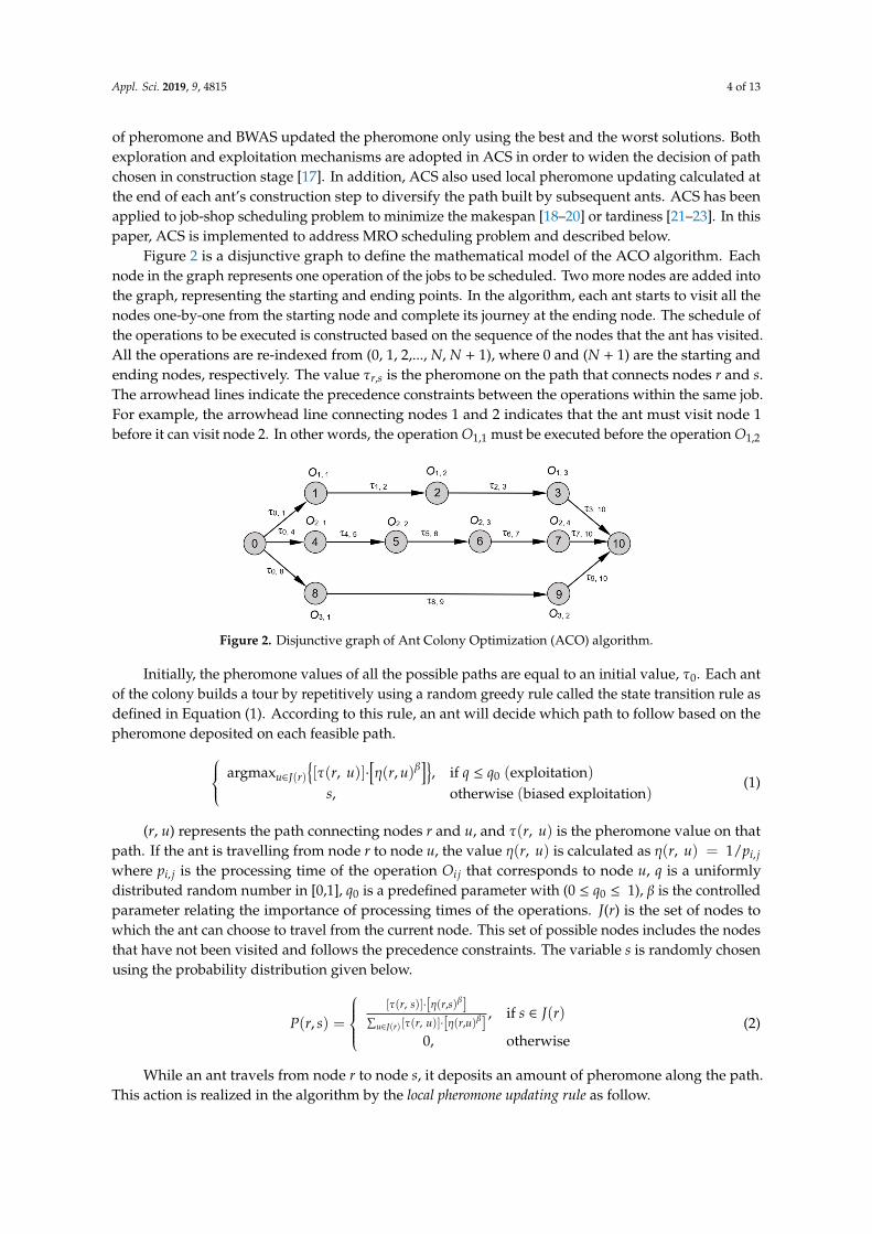
Figure 2 is a disjunctive graph to define the mathematical model of the ACO algorithm. Eachnode in the graph represents one operation of the jobs to be scheduled. Two more nodes are added intothe graph, representing the starting and ending points. In the algorithm, each ant starts to visit all thenodes one-by-one from the starting node and complete its journey at the ending node. The schedule ofthe operations to be executed is constructed based on the sequence of the nodes that the ant has visited.All the operations are re-indexed from (0, 1, 2,..., N, N + 1), where 0 and (N + 1) are the starting andending nodes, respectively. The value τr,s is the pheromone on the path that connects nodes r and s.The arrowhead lines indicate the precedence constraints between the operations within the same job.For example, the arrowhead line connecting nodes 1 and 2 indicates that the ant must visit node 1before it can visit node 2. In other words, the operation O1,1 must be executed before the operation O1,2

Appl. Sci. 2019, 9, x FOR PEER REVIEW 4 of 14

system of subsets of solutions so only these are used for pheromone update. MMAS has bounded value of pheromone and BWAS updated the pheromone only using the best and the worst solutions. Both exploration and exploitation mechanisms are adopted in ACS in order to widen the decision of path chosen in construction stage [17]. In addition, ACS also used local pheromone updating calculated at the end of each ant’s construction step to diversify the path built by subsequent ants. ACS has been applied to job-shop scheduling problem to minimize the makespan [18–20] or tardiness [21–23]. In this paper, ACS is implemented to address MRO scheduling problem and described below.

Figure 2 is a disjunctive graph to define the mathematical model of the ACO algorithm. Each node in the graph represents one operation of the jobs to be scheduled. Two more nodes are added into the graph, representing the starting and ending points. In the algorithm, each ant starts to visit all the nodes one-by-one from the starting node and complete its journey at the ending node. The schedule of the operations to be executed is constructed based on the sequence of the nodes that the ant has visited. All the operations are re-indexed from (0, 1, 2,..., N, N + 1), where 0 and (N + 1) are the starting and ending nodes, respectively. The value , is the pheromone on the path that connects nodes r and s. The arrowhead lines indicate the precedence constraints between the operations within the same job. For example, the arrowhead line connecting nodes 1 and 2 indicates that the ant must visit node 1 before it can visit node 2. In other words, the operation , must be executed before the operation ,

Figure 2. Disjunctive graph of Ant Colony Optimization (ACO) algorithm.

Initially, the pheromone values of all the possible paths are equal to an initial value, τ0. Each ant of the colony builds a tour by repetitively using a random greedy rule called the state transition rule as defined in Eq. (1). According to this rule, an ant will decide which path to follow based on the pheromone deposited on each feasible path. argmax ∈ ( ) ( , ) ∙ ( , ) , if 0(exploitation), otherwise(biasedexploitation) (1)

(r, u) represents the path connecting nodes r and u, and ( , ) is the pheromone value on that path. If the ant is travelling from node r to node u, the value ( , ) is calculated as ( , ) =1/ , where , is the processing time of the operation that corresponds to node u, q is a uniformly distributed random number in [0,1], is a predefined parameter with (0 1), β is the controlled parameter relating the importance of processing times of the operations. J(r) is the set of nodes to which the ant can choose to travel from the current node. This set of possible nodes includes the nodes that have not been visited and follows the precedence constraints. The variable s is randomly chosen using the probability distribution given below.

( , ) = ( , ) ∙ ( , )∑ ( , ) ∙ ( , )∈ ( ) ,0, otherwise if ∈ ( ) (2)

While an ant travels from node r to node s, it deposits an amount of pheromone along the path. This action is realized in the algorithm by the local pheromone updating rule as follow. ( , ) ← (1 − ) ∙ ( , ) + ∙ (3)

where ρ is the local pheromone evaporation rate (0 1).

Figure 2. Disjunctive graph of Ant Colony Optimization (ACO) algorithm.

Initially, the pheromone values of all the possible paths are equal to an initial value, τ0. Each antof the colony builds a tour by repetitively using a random greedy rule called the state transition rule asdefined in Equation (1). According to this rule, an ant will decide which path to follow based on thepheromone deposited on each feasible path. argmaxu∈J(r)

{[τ(r, u)]·

[η(r, u)β

]}, if q ≤ q0 (exploitation)

s, otherwise (biased exploitation)(1)

(r, u) represents the path connecting nodes r and u, and τ(r, u) is the pheromone value on thatpath. If the ant is travelling from node r to node u, the value η(r, u) is calculated as η(r, u) = 1/pi, jwhere pi, j is the processing time of the operation Oi j that corresponds to node u, q is a uniformlydistributed random number in [0,1], q0 is a predefined parameter with (0 ≤ q0 ≤ 1), β is the controlledparameter relating the importance of processing times of the operations. J(r) is the set of nodes towhich the ant can choose to travel from the current node. This set of possible nodes includes the nodesthat have not been visited and follows the precedence constraints. The variable s is randomly chosenusing the probability distribution given below.

P(r, s) =

[τ(r, s)]·[η(r,s)β]∑

u∈J(r) [τ(r, u)]·[η(r,u)β], if s ∈ J(r)

0, otherwise(2)

While an ant travels from node r to node s, it deposits an amount of pheromone along the path.This action is realized in the algorithm by the local pheromone updating rule as follow.

Appl. Sci. 2019, 9, 4815 5 of 13

τ(r, s)← (1− ρ)·τ(r, s) + ρ·τ0 (3)

where ρ is the local pheromone evaporation rate (0 < ρ < 1).Once all the ants of the colony have completed their tours, the schedule to execute the operations

can be built based on the sequence of nodes that each ant has visited during the tour. The operationsare scheduled by following the sequence of the nodes as soon as the required machines are available.Afterwards, the time to complete all the operations of each ant, Cmax, is defined from the schedule.The best tour provides the minimum value of Cmax. Subsequently, the global pheromone updating rule isperformed as follow.

τ(r, s)← (1− α)·τ(r, s) + Q·α·∆τ(r, s) (4)

where

∆τ(r, s) ={ 1

minCmax, if (r, s) ∈ global− best− tour

0, otherwise(5)

α is the global pheromone evaporation rate which control the influence of the new best solution, Q is atuning parameter. With the new updated values of pheromone on all the possible paths, the process,where all the ants build their tours until the global pheromone updating rule is performed, is iterateduntil the solution (Cmax)min converges and the scheduling optimization is completed.

4. Numerical Results

4.1. Minimizing Make-Span

The ACO algorithm explained in previous section has been implemented in MATLAB. The inputincludes all jobs for scheduling, their operations as well as processing time and machine of eachoperation. Users can input the required information into a csv file. Subsequently, the ACO programloads the information from the csv file and executes the optimization algorithm. Once the optimizationoperation has been performed, a schedule or Gantt chart is generated as output.

A use case has been deployed in order to demonstrate the performance of ACO algorithm. Inthis use case, there are 10 components that correspond to 10 jobs to be scheduled. After damages onthese components were identified at an inspection station, the operations of the jobs, their sequences,required machines and processing times were defined as shown in Table 1. These data are also includedin the input file for the algorithm to run. Values of the parameters of algorithm are selected as follows:α = 0.1; ρ = 0.1; β = 0; q0 = 0.8; τ0 = 0.1. Values of the other parameters which are Q and A willbe discussed in the next sub-section as they have significant impacts to performance of the algorithm.

Table 1. Required machines and processing times of operations in the use case to execute theACO algorithm.

Job

Operation Operation 1 Operation 2 Operation 3 Operation 4 Operation 5

Processtime Machine Process

time Machine Processtime Machine Process

time Machine Processtime Machine

Job 1 5 (min) 2 2 (min) 9 3 (min) 10 - - - -

Job 2 2 (min) 1 4 (min) 2 1 (min) 3 - - - -

Job 3 1 (min) 1 4 (min) 3 3 (min) 2 - - - -

Job 4 20 (min) 1 5 (min) 2 16 (min) 3 15 (min) 4 25 (min) 5

Job 5 15 (min) 1 25 (min) 10 - - - - - -

Job 6 15 (min) 6 7 (min) 5 - - - - - -

Job 7 10 (min) 1 7 (min) 2 20 (min) 3 - - - -

Job 8 20 (min) 4 5 (min) 5 16 (min) 6 15 (min) 7 25 (min) 8

Job 9 15 (min) 10 7 (min) 8 - - - - - -

Job 10 15 (min) 3 7 (min) 6 - - - - - -

Appl. Sci. 2019, 9, 4815 6 of 13

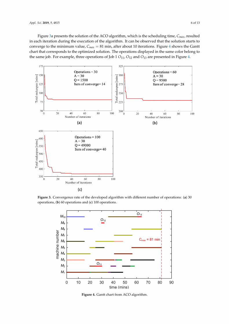
Figure 3a presents the solution of the ACO algorithm, which is the scheduling time, Cmax, resultedin each iteration during the execution of the algorithm. It can be observed that the solution starts toconverge to the minimum value, Cmax = 81 min, after about 10 iterations. Figure 4 shows the Ganttchart that corresponds to the optimized solution. The operations displayed in the same color belong tothe same job. For example, three operations of Job 1 O11, O12 and O13 are presented in Figure 4.

Appl. Sci. 2019, 9, x FOR PEER REVIEW 6 of 14

Job 9 15

(min) 10 7 (min) 8 - - - - - -

Job 10 15

(min) 3 7 (min) 6 - - - - - -

Figure 3a presents the solution of the ACO algorithm, which is the scheduling time, ,

resulted in each iteration during the execution of the algorithm. It can be observed that the solution starts to converge to the minimum value, = 81 , after about 10 iterations. Figure 4 shows the Gantt chart that corresponds to the optimized solution. The operations displayed in the same color belong to the same job. For example, three operations of Job 1 , and are presented in Figure 4.

Figure 3. Convergence rate of the developed algorithm with different number of operations: (a) 30 operations, (b) 60 operations and (c) 100 operations.

Figure 3. Convergence rate of the developed algorithm with different number of operations: (a) 30operations, (b) 60 operations and (c) 100 operations.Appl. Sci. 2019, 9, x FOR PEER REVIEW 7 of 14

Figure 4. Gantt chart from ACO algorithm.

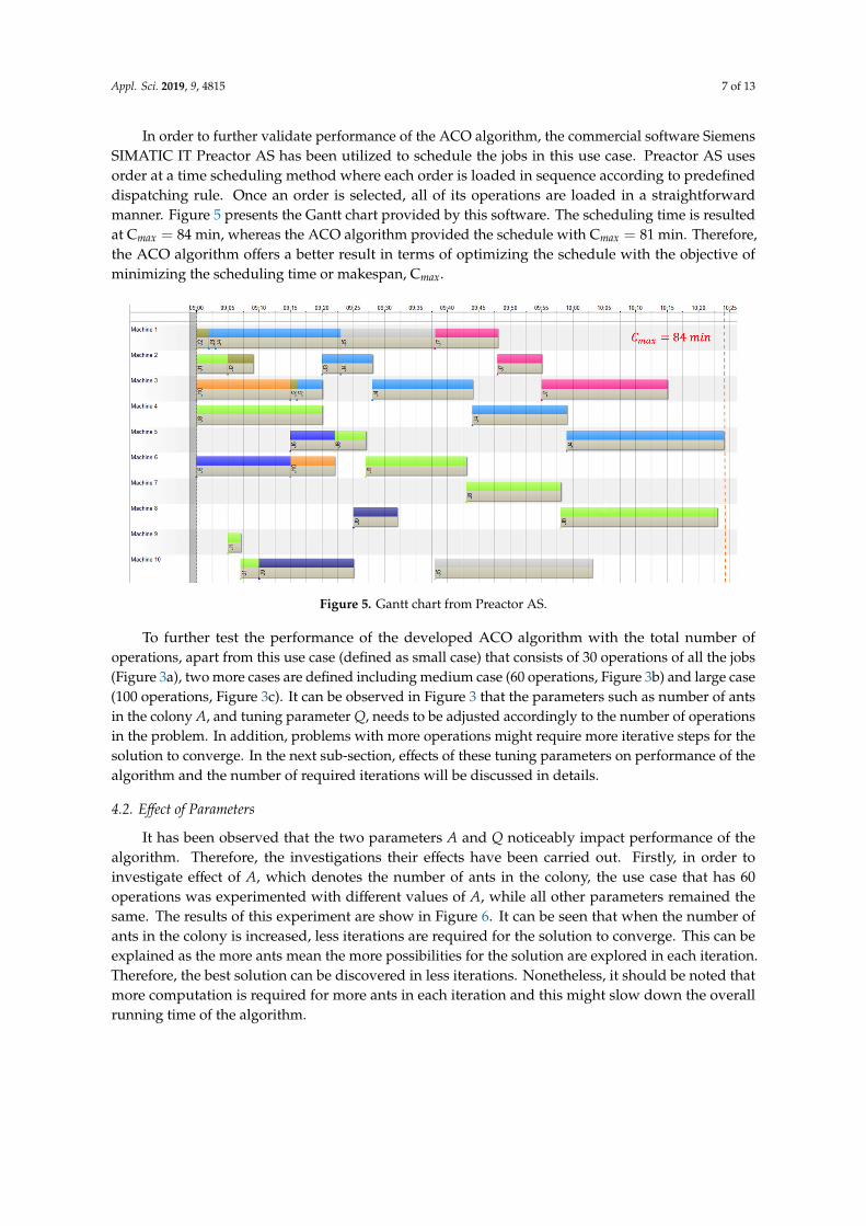
In order to further validate performance of the ACO algorithm, the commercial software Siemens SIMATIC IT Preactor AS has been utilized to schedule the jobs in this use case. Preactor AS uses order at a time scheduling method where each order is loaded in sequence according to predefined dispatching rule. Once an order is selected, all of its operations are loaded in a straightforward manner. Figure 5 presents the Gantt chart provided by this software. The scheduling time is resulted at C = 84min, whereas the ACO algorithm provided the schedule with C =81min. Therefore, the ACO algorithm offers a better result in terms of optimizing the schedule with the objective of minimizing the scheduling time or makespan, C .

Figure 5. Gantt chart from Preactor AS.

To further test the performance of the developed ACO algorithm with the total number of operations, apart from this use case (defined as small case) that consists of 30 operations of all the jobs (Figure 3a), two more cases are defined including medium case (60 operations, Figure 3b) and large case (100 operations, Figure 3c). It can be observed in Figure 3 that the parameters such as number of ants in the colony , and tuning parameter , needs to be adjusted accordingly to the number of operations in the problem. In addition, problems with more operations might require more iterative steps for the solution to converge. In the next sub-section, effects of these tuning parameters on performance of the algorithm and the number of required iterations will be discussed in details.

Figure 4. Gantt chart from ACO algorithm.

Appl. Sci. 2019, 9, 4815 7 of 13

In order to further validate performance of the ACO algorithm, the commercial software SiemensSIMATIC IT Preactor AS has been utilized to schedule the jobs in this use case. Preactor AS usesorder at a time scheduling method where each order is loaded in sequence according to predefineddispatching rule. Once an order is selected, all of its operations are loaded in a straightforwardmanner. Figure 5 presents the Gantt chart provided by this software. The scheduling time is resultedat Cmax = 84 min, whereas the ACO algorithm provided the schedule with Cmax = 81 min. Therefore,the ACO algorithm offers a better result in terms of optimizing the schedule with the objective ofminimizing the scheduling time or makespan, Cmax.

Appl. Sci. 2019, 9, x FOR PEER REVIEW 7 of 14

Figure 4. Gantt chart from ACO algorithm.

In order to further validate performance of the ACO algorithm, the commercial software Siemens SIMATIC IT Preactor AS has been utilized to schedule the jobs in this use case. Preactor AS uses order at a time scheduling method where each order is loaded in sequence according to predefined dispatching rule. Once an order is selected, all of its operations are loaded in a straightforward manner. Figure 5 presents the Gantt chart provided by this software. The scheduling time is resulted at C = 84min, whereas the ACO algorithm provided the schedule with C =81min. Therefore, the ACO algorithm offers a better result in terms of optimizing the schedule with the objective of minimizing the scheduling time or makespan, C .

Figure 5. Gantt chart from Preactor AS.

To further test the performance of the developed ACO algorithm with the total number of operations, apart from this use case (defined as small case) that consists of 30 operations of all the jobs (Figure 3a), two more cases are defined including medium case (60 operations, Figure 3b) and large case (100 operations, Figure 3c). It can be observed in Figure 3 that the parameters such as number of ants in the colony , and tuning parameter , needs to be adjusted accordingly to the number of operations in the problem. In addition, problems with more operations might require more iterative steps for the solution to converge. In the next sub-section, effects of these tuning parameters on performance of the algorithm and the number of required iterations will be discussed in details.

Figure 5. Gantt chart from Preactor AS.

To further test the performance of the developed ACO algorithm with the total number ofoperations, apart from this use case (defined as small case) that consists of 30 operations of all the jobs(Figure 3a), two more cases are defined including medium case (60 operations, Figure 3b) and large case(100 operations, Figure 3c). It can be observed in Figure 3 that the parameters such as number of antsin the colony A, and tuning parameter Q, needs to be adjusted accordingly to the number of operationsin the problem. In addition, problems with more operations might require more iterative steps for thesolution to converge. In the next sub-section, effects of these tuning parameters on performance of thealgorithm and the number of required iterations will be discussed in details.

4.2. Effect of Parameters

It has been observed that the two parameters A and Q noticeably impact performance of thealgorithm. Therefore, the investigations their effects have been carried out. Firstly, in order toinvestigate effect of A, which denotes the number of ants in the colony, the use case that has 60operations was experimented with different values of A, while all other parameters remained thesame. The results of this experiment are show in Figure 6. It can be seen that when the number ofants in the colony is increased, less iterations are required for the solution to converge. This can beexplained as the more ants mean the more possibilities for the solution are explored in each iteration.Therefore, the best solution can be discovered in less iterations. Nonetheless, it should be noted thatmore computation is required for more ants in each iteration and this might slow down the overallrunning time of the algorithm.

Appl. Sci. 2019, 9, 4815 8 of 13

Appl. Sci. 2019, 9, x FOR PEER REVIEW 8 of 14

4.2. Effect of Parameters

It has been observed that the two parameters and noticeably impact performance of the algorithm. Therefore, the investigations their effects have been carried out. Firstly, in order to investigate effect of , which denotes the number of ants in the colony, the use case that has 60 operations was experimented with different values of , while all other parameters remained the same. The results of this experiment are show in Figure 6. It can be seen that when the number of ants in the colony is increased, less iterations are required for the solution to converge. This can be explained as the more ants mean the more possibilities for the solution are explored in each iteration. Therefore, the best solution can be discovered in less iterations. Nonetheless, it should be noted that more computation is required for more ants in each iteration and this might slow down the overall running time of the algorithm.

Figure 6. Tuning Number of Ants parameter, , for a use-case of 60 operations and fixed value of = 9500: (a) = 15, (b) = 30 and (c) = 45

In order to investigate effect of the parameter , the same use case that has 60 operations was also used. Three test cases were experimented with the value of varied, while other parameters were kept the same. The results of these test cases are shown in Figure 7. It can be observed from Figure 7a–c that the higher value of is defined, the lesser iterations are required for the solution to converge. This is because based on Equation (4), the effect of is to amplify the enhancement of pheromone when the global updating rule is applied for the best solution. Therefore, the convergence rate towards the best solution is increased. However, it should be noted that an excessively high value of might lead to a local optimal solution. For example, in Figure 7d, the value of is increased to 50,000 and the best solution found is 240 min, while in the other cases, the best solution found is 230 min.

Figure 6. Tuning Number of Ants parameter, A, for a use-case of 60 operations and fixed value ofQ = 9500: (a) A = 15, (b) A = 30 and (c) A = 45.

In order to investigate effect of the parameter Q, the same use case that has 60 operations was alsoused. Three test cases were experimented with the value of Q varied, while other parameters were keptthe same. The results of these test cases are shown in Figure 7. It can be observed from Figure 7a–c thatthe higher value of Q is defined, the lesser iterations are required for the solution to converge. This isbecause based on Equation (4), the effect of Q is to amplify the enhancement of pheromone when theglobal updating rule is applied for the best solution. Therefore, the convergence rate towards the bestsolution is increased. However, it should be noted that an excessively high value of Q might lead to alocal optimal solution. For example, in Figure 7d, the value of Q is increased to 50,000 and the bestsolution found is 240 min, while in the other cases, the best solution found is 230 min.

4.3. Minimizing Total Weighted Tardiness

In practical use cases, due dates are usually assigned for work orders. Therefore, in other toconsider this feature, the developed algorithm is tested with another performance objective which isminimizing the total weighted tardiness defined as:∑

wiTi (6)

where wi is the weightage of job i. Ti = max{0, Ci − di} is tardiness of job i, Ci and di are completion timeand due date respectively. In this case study, the weightage of all jobs is set to be equal to each other. Theinput data of machines, operations and processing time is obtained from the minimizing make-span case.The due date is set based on due date tightness factor which is also fixed value for all jobs [21].

Appl. Sci. 2019, 9, 4815 9 of 13Appl. Sci. 2019, 9, x FOR PEER REVIEW 9 of 14

Figure 7. Tuning parameter Q for a use-case of 60 operations and fixed value of parameter = 30: (a) = 7000, (b) = 9500, (c) = 11,000 and (d) = 50,000

4.3. Minimizing Total Weighted Tardiness

In practical use cases, due dates are usually assigned for work orders. Therefore, in other to consider this feature, the developed algorithm is tested with another performance objective which is minimizing the total weighted tardiness defined as:

(6)

where is the weightage of job . = max 0, − is tardiness of job , and are completion time and due date respectively. In this case study, the weightage of all jobs is set to be equal to each other. The input data of machines, operations and processing time is obtained from the minimizing make-span case. The due date is set based on due date tightness factor which is also fixed value for all jobs [21].

Similar to minimizing the make span, three cases with variable number of operations: small (30 operations), medium (60 operations) and large (100 operations) are used to test the developed algorithm. The tuning parameters are the same as previous simulation, which are number of ants in the colony A and parameter Q.

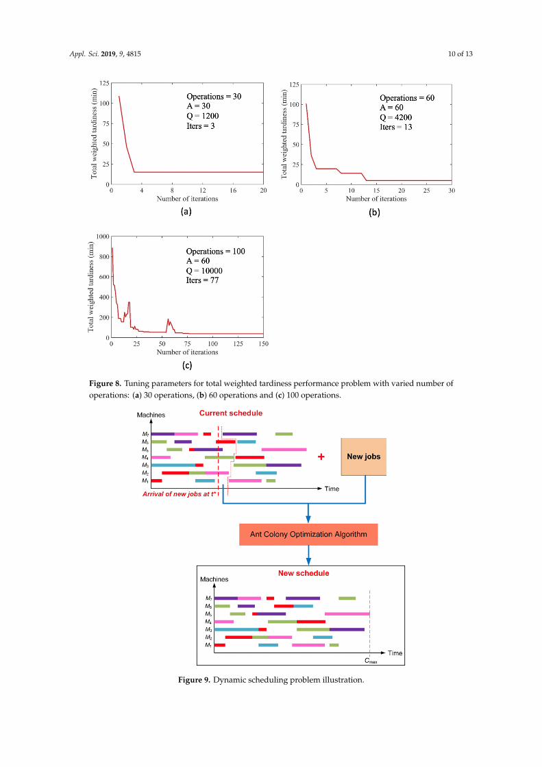
The convergence graphs of the problems with different numbers of operations and the parameters adjusted are presented in Figure 8. When we increase the number of operations, different combinations of A and Q are needed to ensure converged solutions. Small value of A = 30 and Q = 1200 are sufficient for small number of operations. However, for larger size problem, the number of ants A and Q should be increased. Large value of A requires more computing time; therefore, for the largest number of operations, increasing Q is preferred to speed up the running time.

Figure 7. Tuning parameter Q for a use-case of 60 operations and fixed value of parameter A = 30: (a)Q = 7000, (b) Q = 9500, (c) Q = 11, 000 and (d) Q = 50, 000.

Similar to minimizing the make span, three cases with variable number of operations: small(30 operations), medium (60 operations) and large (100 operations) are used to test the developedalgorithm. The tuning parameters are the same as previous simulation, which are number of ants inthe colony A and parameter Q.

The convergence graphs of the problems with different numbers of operations and the parametersadjusted are presented in Figure 8. When we increase the number of operations, different combinationsof A and Q are needed to ensure converged solutions. Small value of A = 30 and Q = 1200 are sufficientfor small number of operations. However, for larger size problem, the number of ants A and Q shouldbe increased. Large value of A requires more computing time; therefore, for the largest number ofoperations, increasing Q is preferred to speed up the running time.

4.4. Dynamic scheduling

We have extended the ACO to solve the problem of dynamic scheduling or re-scheduling. Inpractical scenarios, during the execution of the scheduled jobs, there are usually arrivals of new orurgent work orders that need to be executed at the same time with the on-going work orders. Therefore,the current schedule needs to be updated in order to include new jobs. The ACO algorithm wasdeveloped to accommodate this requirement. Assuming that during the execution process, there arenew jobs arriving at the shop floor at the time point t*. The solver firstly extracts the operations thathave not been started from current schedule. Then, the ACO algorithm is implemented for theseoperations together with the new jobs in order to produce a new updated schedule. This process issummarized in Figure 9.

Appl. Sci. 2019, 9, 4815 10 of 13Appl. Sci. 2019, 9, x FOR PEER REVIEW 10 of 14

Figure 8. Tuning parameters for total weighted tardiness performance problem with varied number of operations: (a) 30 operations, (b) 60 operations and (c) 100 operations.

4.4. Dynamic scheduling

We have extended the ACO to solve the problem of dynamic scheduling or re-scheduling. In practical scenarios, during the execution of the scheduled jobs, there are usually arrivals of new or urgent work orders that need to be executed at the same time with the on-going work orders. Therefore, the current schedule needs to be updated in order to include new jobs. The ACO algorithm was developed to accommodate this requirement. Assuming that during the execution process, there are new jobs arriving at the shop floor at the time point t*. The solver firstly extracts the operations that have not been started from current schedule. Then, the ACO algorithm is implemented for these operations together with the new jobs in order to produce a new updated schedule. This process is summarized in Figure 9.

Figure 8. Tuning parameters for total weighted tardiness performance problem with varied number ofoperations: (a) 30 operations, (b) 60 operations and (c) 100 operations.Appl. Sci. 2019, 9, x FOR PEER REVIEW 11 of 14

Figure 9. Dynamic scheduling problem illustration.

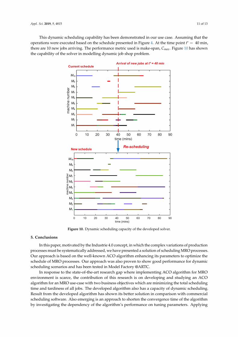
This dynamic scheduling capability has been demonstrated in our use case. Assuming that the operations were executed based on the schedule presented in Figure 4. At the time point ∗ =40 , there are 10 new jobs arriving. The performance metric used is make-span, . Figure 10 has shown the capability of the solver in modelling dynamic job shop problem.

Figure 9. Dynamic scheduling problem illustration.

Appl. Sci. 2019, 9, 4815 11 of 13

This dynamic scheduling capability has been demonstrated in our use case. Assuming that theoperations were executed based on the schedule presented in Figure 4. At the time point t∗ = 40 min,there are 10 new jobs arriving. The performance metric used is make-span, Cmax. Figure 10 has shownthe capability of the solver in modelling dynamic job shop problem.Appl. Sci. 2019, 9, x FOR PEER REVIEW 12 of 14

Figure 10. Dynamic scheduling capacity of the developed solver.

5. Conclusions

In this paper, motivated by the Industrie 4.0 concept, in which the complex variations of production processes must be systematically addressed, we have presented a solution of scheduling MRO processes. Our approach is based on the well-known ACO algorithm enhancing its parameters to optimize the schedule of MRO processes. Our approach was also proven to show good performance for dynamic scheduling scenarios and has been tested in Model Factory @ARTC.

In response to the state-of-the-art research gap where implementing ACO algorithm for MRO environment is scarce, the contribution of this research is on developing and studying an ACO algorithm for an MRO use-case with two business objectives which are minimizing the total scheduling time and tardiness of all jobs. The developed algorithm also has a capacity of dynamic scheduling. Result from the developed algorithm has shown its better solution in comparison with commercial scheduling software. Also emerging is an approach to shorten the convergence time of the algorithm by investigating the dependency of the algorithm’s performance on tuning parameters. Applying the developed ACO algorithm in this research can bring out various practical business values to companies. For example, complex MRO processes with various product routings can be optimally scheduled to improve productivity. The dynamic scheduling capability developed in this study can help production planners efficiently adjust the current product schedules to accommodate urgent work orders or additional work orders induced during the production process which frequently occurs in the MRO environment.

Figure 10. Dynamic scheduling capacity of the developed solver.

5. Conclusions

In this paper, motivated by the Industrie 4.0 concept, in which the complex variations of productionprocesses must be systematically addressed, we have presented a solution of scheduling MRO processes.Our approach is based on the well-known ACO algorithm enhancing its parameters to optimize theschedule of MRO processes. Our approach was also proven to show good performance for dynamicscheduling scenarios and has been tested in Model Factory @ARTC.

In response to the state-of-the-art research gap where implementing ACO algorithm for MROenvironment is scarce, the contribution of this research is on developing and studying an ACOalgorithm for an MRO use-case with two business objectives which are minimizing the total schedulingtime and tardiness of all jobs. The developed algorithm also has a capacity of dynamic scheduling.Result from the developed algorithm has shown its better solution in comparison with commercialscheduling software. Also emerging is an approach to shorten the convergence time of the algorithmby investigating the dependency of the algorithm’s performance on tuning parameters. Applying

Appl. Sci. 2019, 9, 4815 12 of 13

the developed ACO algorithm in this research can bring out various practical business values tocompanies. For example, complex MRO processes with various product routings can be optimallyscheduled to improve productivity. The dynamic scheduling capability developed in this study canhelp production planners efficiently adjust the current product schedules to accommodate urgent workorders or additional work orders induced during the production process which frequently occurs inthe MRO environment.

There are several areas where the research can be carried on in the future. First, the algorithm canbe improved to shorten the overall time required for the solution to converge. One of the possibilitiesis to modify the local and global pheromone updating strategies. Industrial applicability of thedeveloped algorithm can be enhanced by considering more constraints such as sequence-dependentsetup times, availabilities of materials and personnel. The integration of the developed algorithm tocommercial scheduling software to harvest all advantages of the algorithm and the software is alsounder consideration with the support of middleware option [24]. Finally, alternative optimizationalgorithms such as bee colony for scheduling optimization will be also explored and developed.

Author Contributions: Conceptualization, L.V.T. and B.H.H.; methodology, L.V.T. and B.H.H; software, L.V.T.;validation, L.V.T, B.H.H. and H.A.; formal analysis, L.V.T. and B.H.H.; investigation, L.V.T.; resources, B.H.H. andH.A.; data curation, L.V.T.; writing—original draft preparation, L.V.T.; writing—review and editing, L.V.T, B.H.H.and H.A.; visualization, L.V.T. and B.H.H.; supervision, H.A.; project administration, B.H.H. and H.A.; fundingacquisition, H.A.

Funding: This research is supported by the Agency for Science, Technology and Research (A*STAR) under itsAdvanced Manufacturing & Engineering (AME) Industry Alignment Funding - Pre-positioning funding scheme(Project No: A1723a0035).

Conflicts of Interest: The authors declare no conflict of interest.

References

1. Roy, R.; Stark, R.; Tracht, K.; Takata, S.; Mori, M. Continuous maintenance and the future–Foundations andtechnological challenges. Cirp Ann. 2016, 65, 667–688. [CrossRef]

2. Coro, A.; Abasolo, M.; Aguirrebeitia, J.; Lopez de Lacalle, L.N. Inspection scheduling based on reliabilityupdating of gas turbine welded structures. Adv. Mech. Eng. 2019, 11, 1–20. [CrossRef]

3. Coro, A.; Macareno, L.M.; Aguirrebeitia, J.; López de Lacalle, L.N. A Methodology to Evaluate the ReliabilityImpact of the Replacement of Welded Components by Additive Manufacturing Spare Parts. Metals 2019, 9,932. [CrossRef]

4. Liu, P.; Zhang, X.; Shi, Z.; Huang, Z. Simulation Optimization for MRO Systems Operations. Asia-Pac. J.Oper. Res. 2017, 34, 1750003. [CrossRef]

5. Toader, F.A. Production scheduling in flexible manufacturing systems: A state of the art survey. J. Electr. Eng.Electron. Control Comput. Sci. 2017, 3, 1–6.

6. Mavrovouniotis, M.; Li, C.; Yang, S. A survey of swarm intelligence for dynamic optimization: Algorithmsand applications. Swarm Evol. Comput. 2017, 33, 1–17. [CrossRef]

7. Lin, C.W.; Lin, Y.K.; Hsieh, H.T. Ant colony optimization for unrelated parallel machine scheduling. Int. J.Adv. Manuf. Technol. 2013, 67, 35–45. [CrossRef]

8. Huang, Z.; Ding, J.; Song, J.; Shi, L.; Chen, C.H. Simulation optimization for the MRO scheduling problembased on multi-fidelity models. In Proceedings of the 2016 IEEE International Conference on IndustrialTechnology (ICIT), Taipei, Taiwan, 14–17 March 2016; pp. 1556–1561.

9. Li, H.; Mi, S.; Li, Q.; Wen, X.; Qiao, D.; Luo, G. A scheduling optimization method for maintenance, repairand operations service resources of complex products. J. Intell. Manuf. 2018, 1–19. [CrossRef]

10. Posada, J.; Toro, C.; Barandiaran, I.; Oyarzun, D.; Stricker, D.; de Amicis, R.; Pinto, E.B.; Eisert, P.; Döllner, J.;Vallarino, I. Visual computing as a key enabling technology for industrie 4.0 and industrial internet. IEEEComput. Graph. Appl. 2015, 35, 26–40. [CrossRef] [PubMed]

11. Dorigo, M.; Birattari, M. Ant Colony Optimization; Springer: Boston, MA, USA, 2010.12. Dorigo, M.; Stützle, T. Ant colony optimization: Overview and recent advances. In Handbook of Metaheuristics;

Springer: Cham, Switzerland, 2019; pp. 311–351.

Appl. Sci. 2019, 9, 4815 13 of 13

13. Zhang, J.; Hu, X.; Tan, X.; Zhong, J.H.; Huang, Q. Implementation of an ant colony optimization techniquefor job shop scheduling problem. Trans. Inst. Meas. Control 2006, 28, 93–108. [CrossRef]

14. Dorigo, M.; Maniezzo, V.; Colorni, A. Ant system: Optimization by a colony of cooperating agents. IEEETrans. Syst. Man Cybern. Part B Cybern. 1996, 26, 29–41. [CrossRef]

15. Dorigo, M.; Dorigo, M.; Manjezzo, V.; Trubian, M. Ant system for job-shop scheduling. Belg. J. Oper. Res.1994, 34, 39–53.

16. Neto, R.F.T.; Godinho Filho, M. Literature review regarding Ant Colony Optimization applied to schedulingproblems: Guidelines for implementation and directions for future research. Eng. Appl. Artif. Intell. 2013, 26,150–161. [CrossRef]

17. Zhuo, X.L.; Zhang, J.; Cheng, W.N. A new pheromone design in ACS for solving JSP. In Proceedings of the2007 IEEE Congress on Evolutionary Computation, Singapore, 25–28 September 2007; pp. 1963–1969.

18. Yagmahan, B.; Yenisey, M.M. Ant colony optimization for multi-objective flow shop scheduling problem.Comput. Ind. Eng. 2008, 54, 411–420. [CrossRef]

19. Wang, L.; Cai, J.; Li, M.; Liu, Z. Flexible job shop scheduling problem using an improved ant colonyoptimization. Sci. Program. 2017, 2017, 9016303. [CrossRef]

20. Qin, W.; Zhang, J.; Song, D. An improved ant colony algorithm for dynamic hybrid flow shop schedulingwith uncertain processing time. J. Intell. Manuf. 2018, 29, 891–904. [CrossRef]

21. Raghavan, N.S.; Venkataramana, M. Parallel processor scheduling for minimizing total weighted tardinessusing ant colony optimization. Int. J. Adv. Manuf. Technol. 2009, 41, 986. [CrossRef]

22. M’Hallah, R.; Alhajraf, A. Ant colony systems for the single-machine total weighted earliness tardinessscheduling problem. J. Sched. 2016, 19, 191–205. [CrossRef]

23. Huang, R.H.; Yu, S.C. Enhancement of job shop scheduling with time windows using a wise select ant colonyoptimization. J. Stat. Manag. Syst. 2015, 18, 57–83. [CrossRef]

24. Modoni, G.E.; Trombetta, A.; Veniero, M.; Sacco, M.; Mourtzis, D. An event-driven integrative frameworkenabling information notification among manufacturing resources. Int. J. Comput. Integr. Manuf. 2019, 32,241–252. [CrossRef]

© 2019 by the authors. Licensee MDPI, Basel, Switzerland. This article is an open accessarticle distributed under the terms and conditions of the Creative Commons Attribution(CC BY) license (http://creativecommons.org/licenses/by/4.0/).