Ansys Tutorial 8 Mixing Tank - drahmednagib.comdrahmednagib.com/onewebmedia/Optimum-Design-2016/Tut v 15/Tutorial_8... · Ansys Tutorial 8 Mixing Tank Optimum Design Course Fall 2016

1

Ansys Tutorial 8

Mixing Tank

Optimum Design Course

Fall 2016

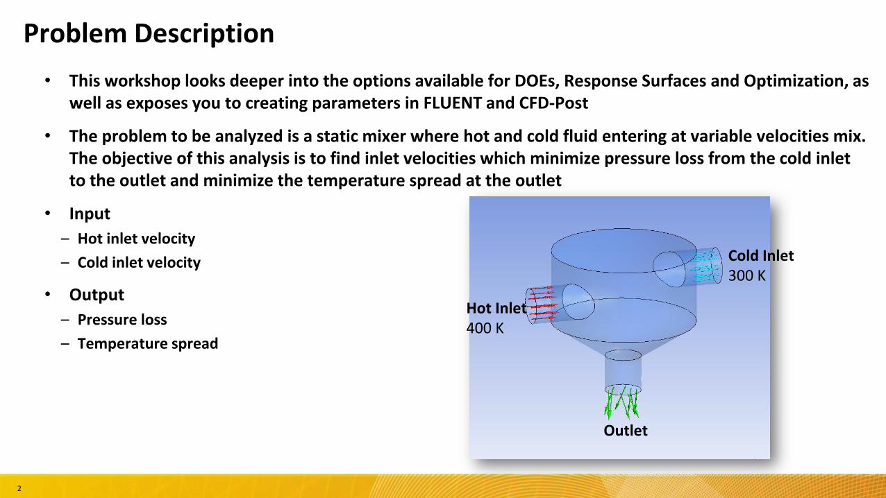
• This workshop looks deeper into the options available for DOEs, Response Surfaces and Optimization, as well as exposes you to creating parameters in FLUENT and CFD-Post

• The problem to be analyzed is a static mixer where hot and cold fluid entering at variable velocities mix. The objective of this analysis is to find inlet velocities which minimize pressure loss from the cold inlet to the outlet and minimize the temperature spread at the outlet

• Input

– Hot inlet velocity

– Cold inlet velocity

• Output

– Pressure loss

– Temperature spread

Cold Inlet300 K

Hot Inlet400 K

Outlet

Problem Description

2

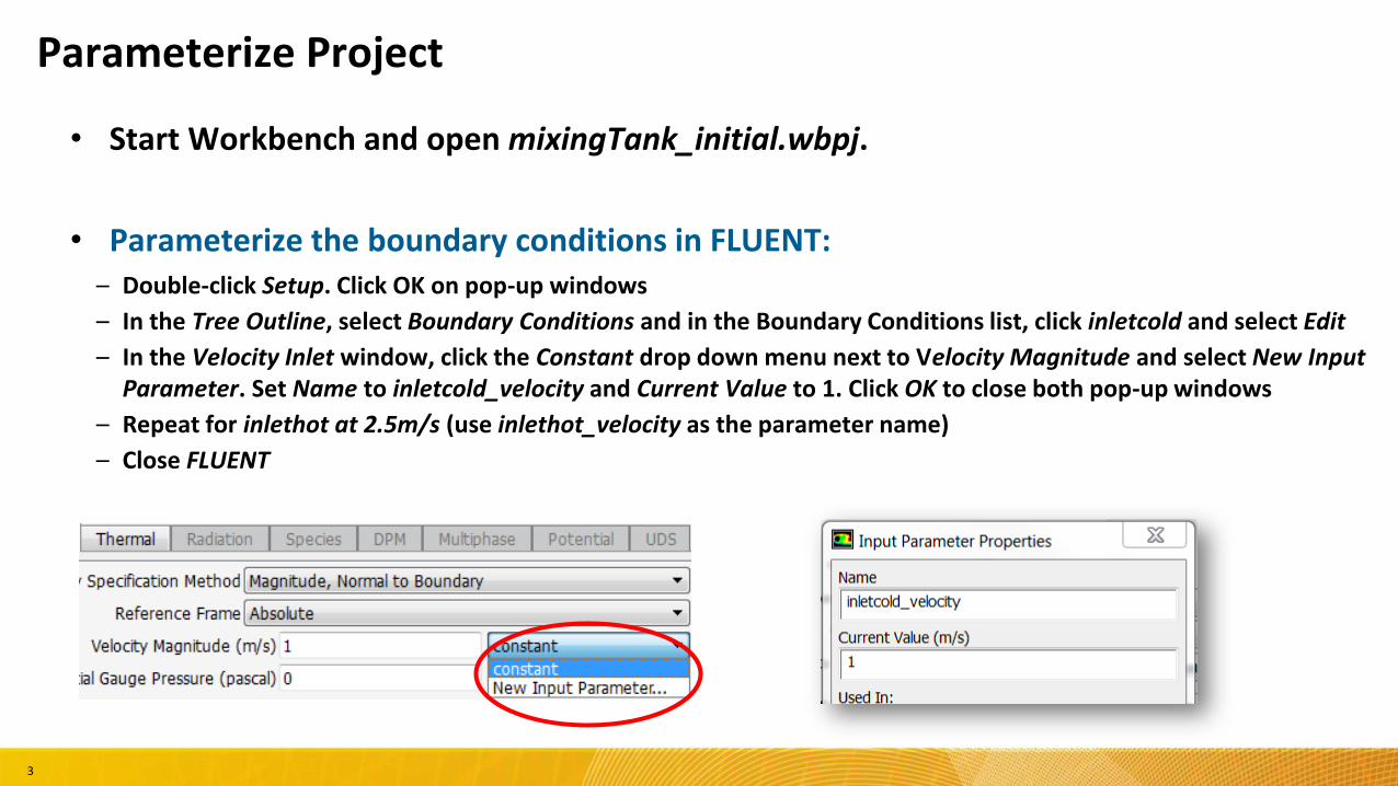
• Parameterize the boundary conditions in FLUENT:– Double-click Setup. Click OK on pop-up windows

– In the Tree Outline, select Boundary Conditions and in the Boundary Conditions list, click inletcold and select Edit

– In the Velocity Inlet window, click the Constant drop down menu next to Velocity Magnitude and select New Input Parameter. Set Name to inletcold_velocity and Current Value to 1. Click OK to close both pop-up windows

– Repeat for inlethot at 2.5m/s (use inlethot_velocity as the parameter name)

– Close FLUENT

Parameterize Project

3

• Start Workbench and open mixingTank_initial.wbpj.

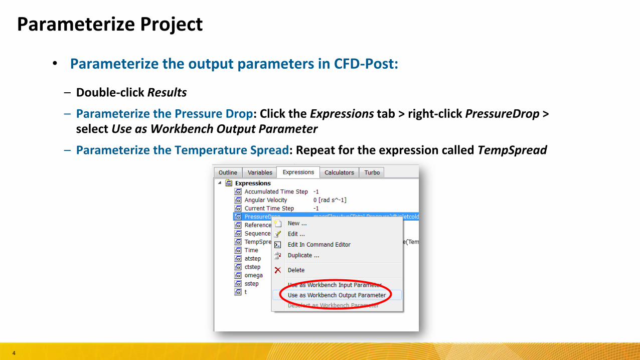
• Parameterize the output parameters in CFD-Post:

– Double-click Results

– Parameterize the Pressure Drop: Click the Expressions tab > right-click PressureDrop > select Use as Workbench Output Parameter

– Parameterize the Temperature Spread: Repeat for the expression called TempSpread

Parameterize Project

4

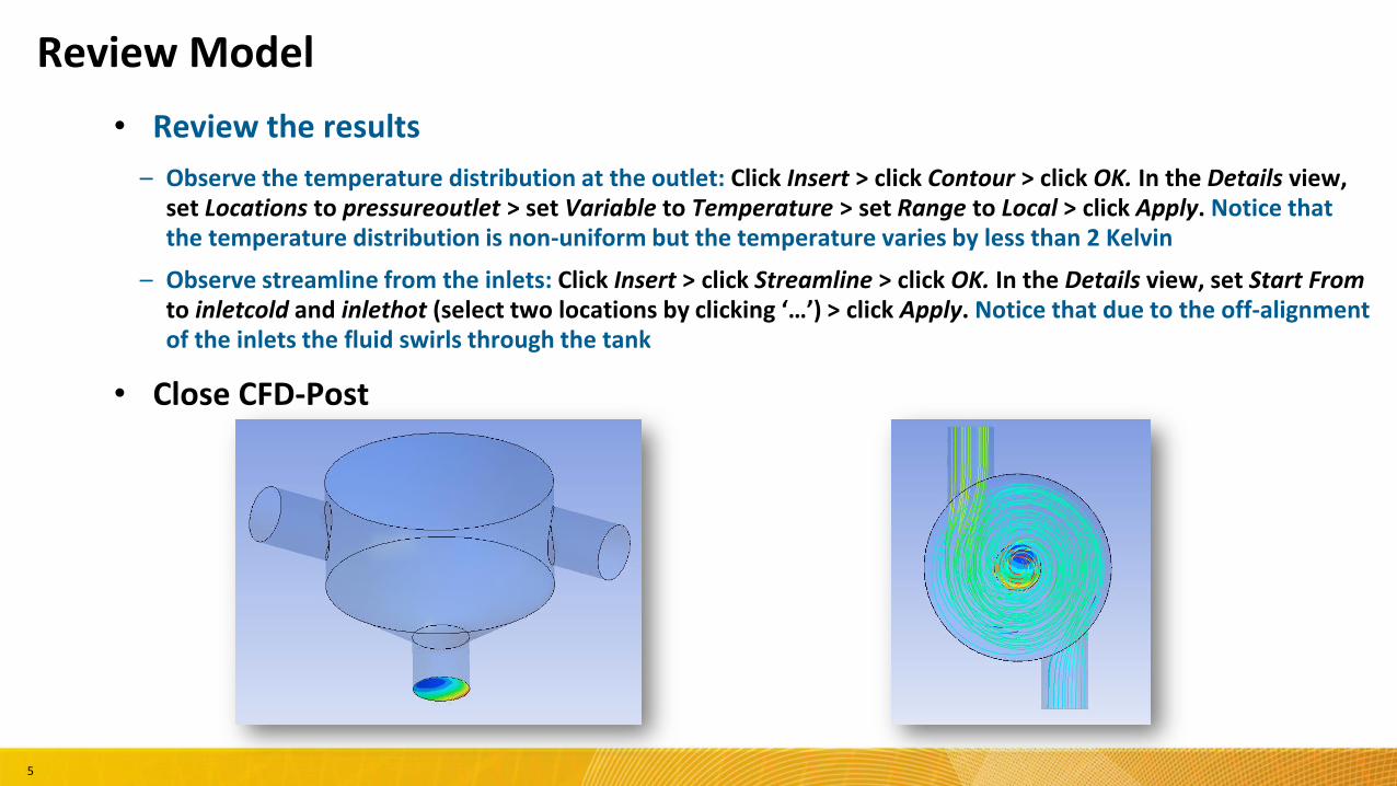
– Observe the temperature distribution at the outlet: Click Insert > click Contour > click OK. In the Details view, set Locations to pressureoutlet > set Variable to Temperature > set Range to Local > click Apply. Notice that the temperature distribution is non-uniform but the temperature varies by less than 2 Kelvin

– Observe streamline from the inlets: Click Insert > click Streamline > click OK. In the Details view, set Start From to inletcold and inlethot (select two locations by clicking ‘…’) > click Apply. Notice that due to the off-alignment of the inlets the fluid swirls through the tank

• Close CFD-Post

Review Model

• Review the results

5

• Drag and drop a Response Surface Optimization system onto the Project Schematic > double-click Design of Experiments

• Explore the different DOE types

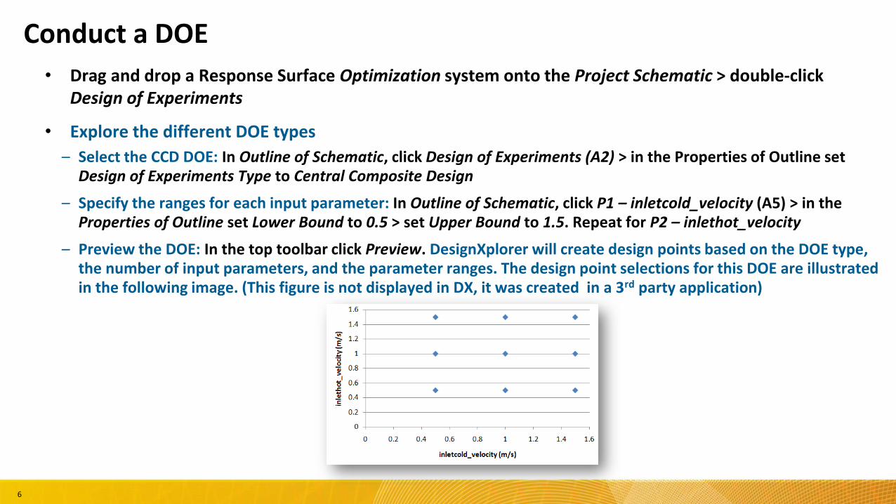
– Select the CCD DOE: In Outline of Schematic, click Design of Experiments (A2) > in the Properties of Outline set Design of Experiments Type to Central Composite Design

– Specify the ranges for each input parameter: In Outline of Schematic, click P1 – inletcold_velocity (A5) > in the Properties of Outline set Lower Bound to 0.5 > set Upper Bound to 1.5. Repeat for P2 – inlethot_velocity

– Preview the DOE: In the top toolbar click Preview. DesignXplorer will create design points based on the DOE type, the number of input parameters, and the parameter ranges. The design point selections for this DOE are illustrated in the following image. (This figure is not displayed in DX, it was created in a 3rd party application)

Conduct a DOE

6

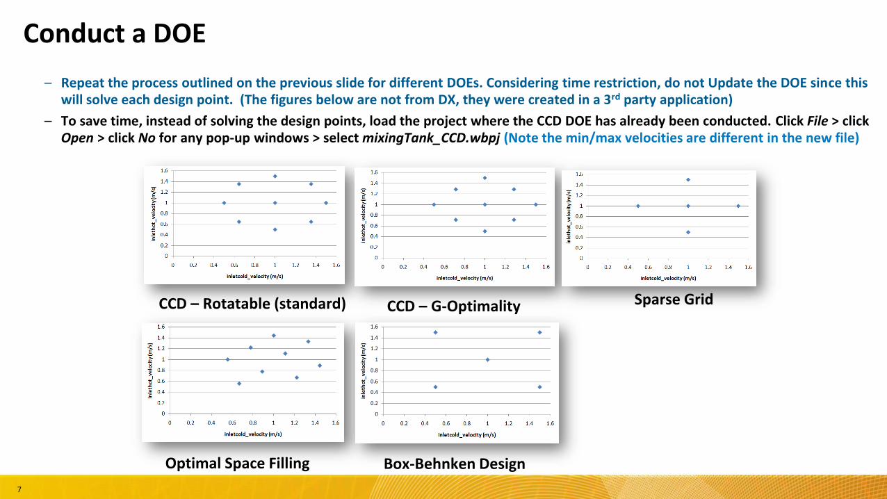
– Repeat the process outlined on the previous slide for different DOEs. Considering time restriction, do not Update the DOE since this will solve each design point. (The figures below are not from DX, they were created in a 3rd party application)

– To save time, instead of solving the design points, load the project where the CCD DOE has already been conducted. Click File > click Open > click No for any pop-up windows > select mixingTank_CCD.wbpj (Note the min/max velocities are different in the new file)

CCD – Rotatable (standard) CCD – G-Optimality

Optimal Space Filling Box-Behnken Design

Sparse Grid

Conduct a DOE

7

• Review the Full 2nd Order Polynomials response surface

– Generate the Full 2nd Order Polynomials Response Surface:

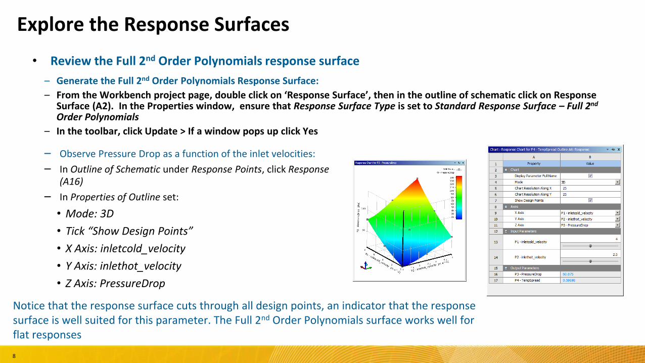
– From the Workbench project page, double click on ‘Response Surface’, then in the outline of schematic click on Response Surface (A2). In the Properties window, ensure that Response Surface Type is set to Standard Response Surface – Full 2nd

Order Polynomials

– In the toolbar, click Update > If a window pops up click Yes

– Observe Pressure Drop as a function of the inlet velocities:

– In Outline of Schematic under Response Points, click Response (A16)

– In Properties of Outline set:

• Mode: 3D

• Tick “Show Design Points”

• X Axis: inletcold_velocity

• Y Axis: inlethot_velocity

• Z Axis: PressureDrop

Notice that the response surface cuts through all design points, an indicator that the response surface is well suited for this parameter. The Full 2nd Order Polynomials surface works well for flat responses

Explore the Response Surfaces

8

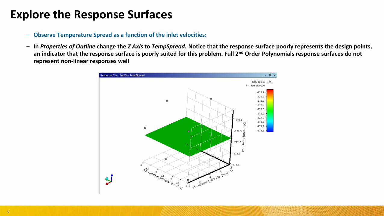
– Observe Temperature Spread as a function of the inlet velocities:

– In Properties of Outline change the Z Axis to TempSpread. Notice that the response surface poorly represents the design points, an indicator that the response surface is poorly suited for this problem. Full 2nd Order Polynomials response surfaces do not represent non-linear responses well


9

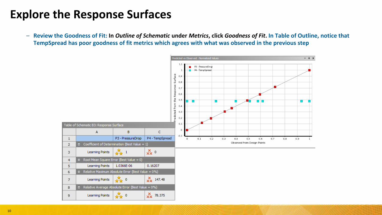
– Review the Goodness of Fit: In Outline of Schematic under Metrics, click Goodness of Fit. In Table of Outline, notice that TempSpread has poor goodness of fit metrics which agrees with what was observed in the previous step


10

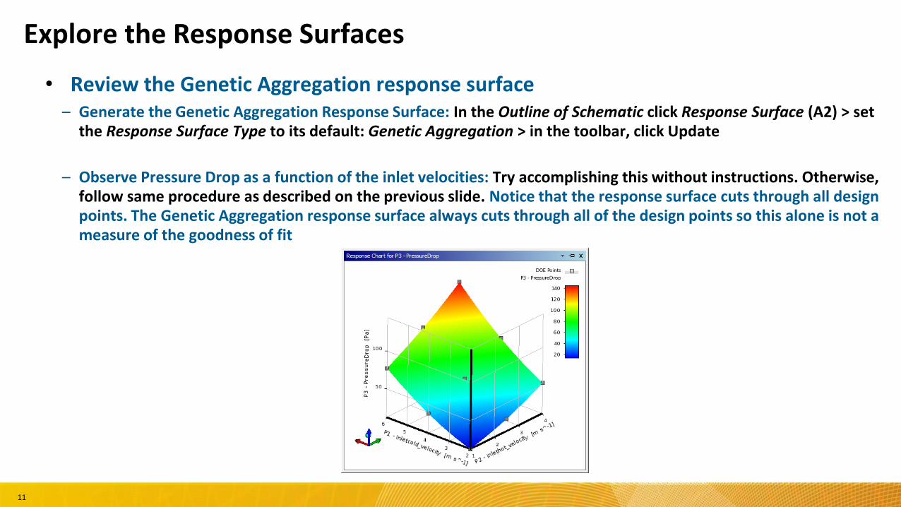
• Review the Genetic Aggregation response surface– Generate the Genetic Aggregation Response Surface: In the Outline of Schematic click Response Surface (A2) > set

the Response Surface Type to its default: Genetic Aggregation > in the toolbar, click Update

– Observe Pressure Drop as a function of the inlet velocities: Try accomplishing this without instructions. Otherwise, follow same procedure as described on the previous slide. Notice that the response surface cuts through all design points. The Genetic Aggregation response surface always cuts through all of the design points so this alone is not a measure of the goodness of fit


11

– Observe Temperature Spread as a function of the inlet velocities (same workflow as before): The Genetic Aggregation response surface cuts through all design points. If the response surface does not pass through all points, try increasing the Number of Points on X and Y

– Review the Goodness of Fit: Since the Genetic Aggregation response surface cuts through all design points, the goodness of fit metrics are always perfect. This, however, does not imply that the response surface properly predicts the response away from the design points. One way to check the goodness of fit for Genetic Aggregation response surfaces is to look at the Cross-Validation on Learning Points and to compare it with one or more verification points. Verification points are additional design points that are not used when generating the response surface, consequently the response surface will not necessarily cut through the verification points (the same applies to the Sparse Grid and Kriging response surfaces)


12

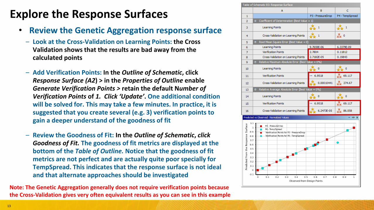
• Review the Genetic Aggregation response surface– Look at the Cross-Validation on Learning Points: the Cross

Validation shows that the results are bad away from the calculated points

– Add Verification Points: In the Outline of Schematic, click Response Surface (A2) > in the Properties of Outline enable Generate Verification Points > retain the default Number of Verification Points of 1. Click ‘Update’. One additional condition will be solved for. This may take a few minutes. In practice, it is suggested that you create several (e.g. 3) verification points to gain a deeper understand of the goodness of fit

– Review the Goodness of Fit: In the Outline of Schematic, click Goodness of Fit. The goodness of fit metrics are displayed at the bottom of the Table of Outline. Notice that the goodness of fit metrics are not perfect and are actually quite poor specially for TempSpread. This indicates that the response surface is not ideal and that alternate approaches should be investigated


Note: The Genetic Aggregation generally does not require verification points becausethe Cross-Validation gives very often equivalent results as you can see in this example

13

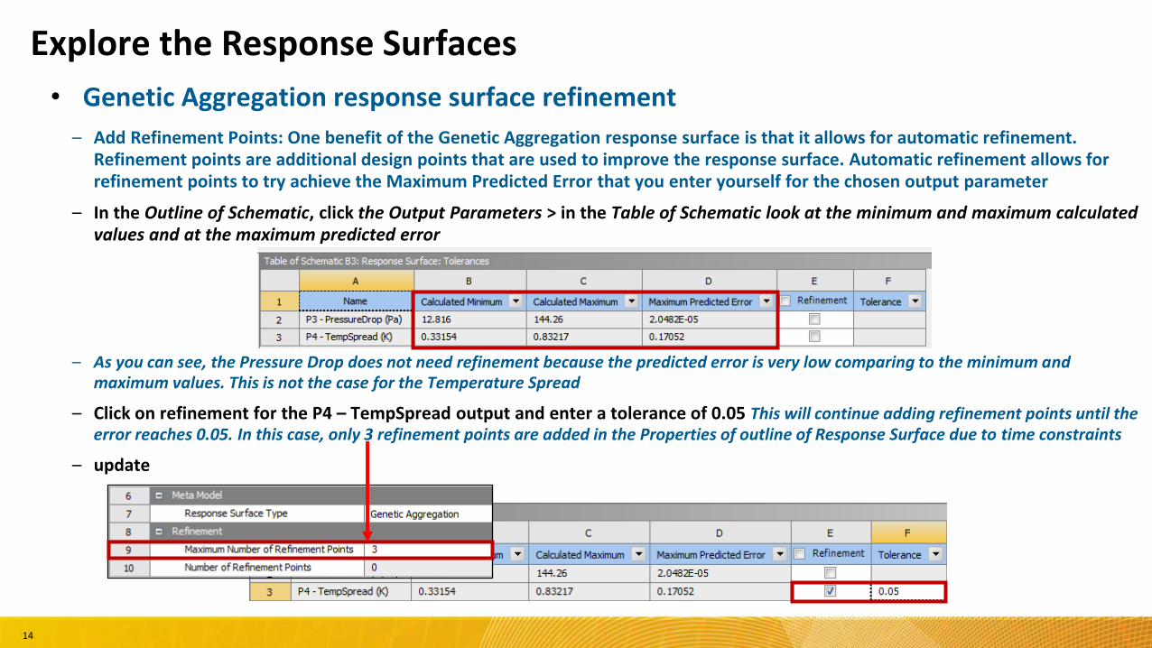
– Add Refinement Points: One benefit of the Genetic Aggregation response surface is that it allows for automatic refinement. Refinement points are additional design points that are used to improve the response surface. Automatic refinement allows forrefinement points to try achieve the Maximum Predicted Error that you enter yourself for the chosen output parameter

– In the Outline of Schematic, click the Output Parameters > in the Table of Schematic look at the minimum and maximum calculated values and at the maximum predicted error

– As you can see, the Pressure Drop does not need refinement because the predicted error is very low comparing to the minimum and maximum values. This is not the case for the Temperature Spread

– Click on refinement for the P4 – TempSpread output and enter a tolerance of 0.05 This will continue adding refinement points until the error reaches 0.05. In this case, only 3 refinement points are added in the Properties of outline of Response Surface due to time constraints

– update


• Genetic Aggregation response surface refinement

14

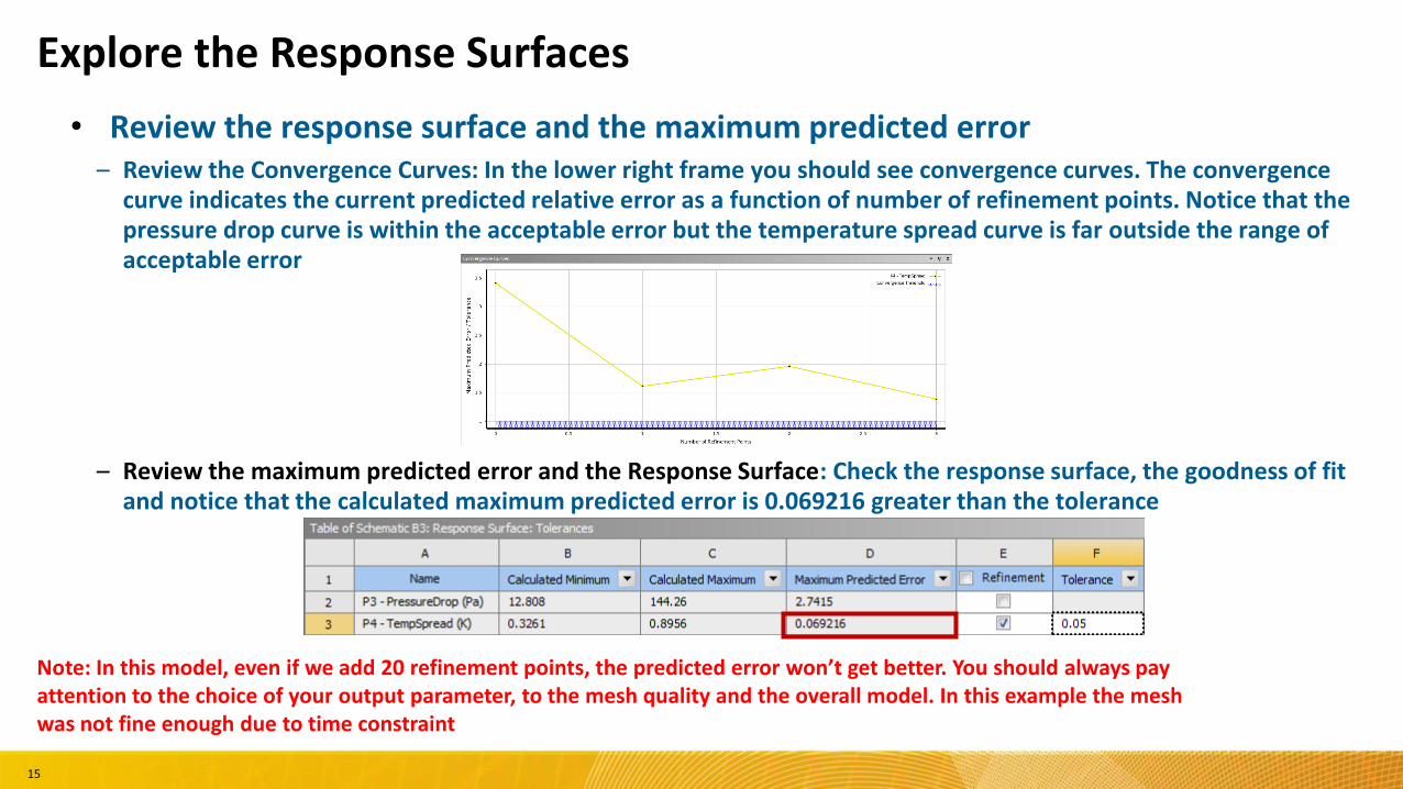
• Review the response surface and the maximum predicted error– Review the Convergence Curves: In the lower right frame you should see convergence curves. The convergence

curve indicates the current predicted relative error as a function of number of refinement points. Notice that the pressure drop curve is within the acceptable error but the temperature spread curve is far outside the range of acceptable error

– Review the maximum predicted error and the Response Surface: Check the response surface, the goodness of fit and notice that the calculated maximum predicted error is 0.069216 greater than the tolerance


Note: In this model, even if we add 20 refinement points, the predicted error won’t get better. You should always payattention to the choice of your output parameter, to the mesh quality and the overall model. In this example the meshwas not fine enough due to time constraint

15

• Review the local sensitivity

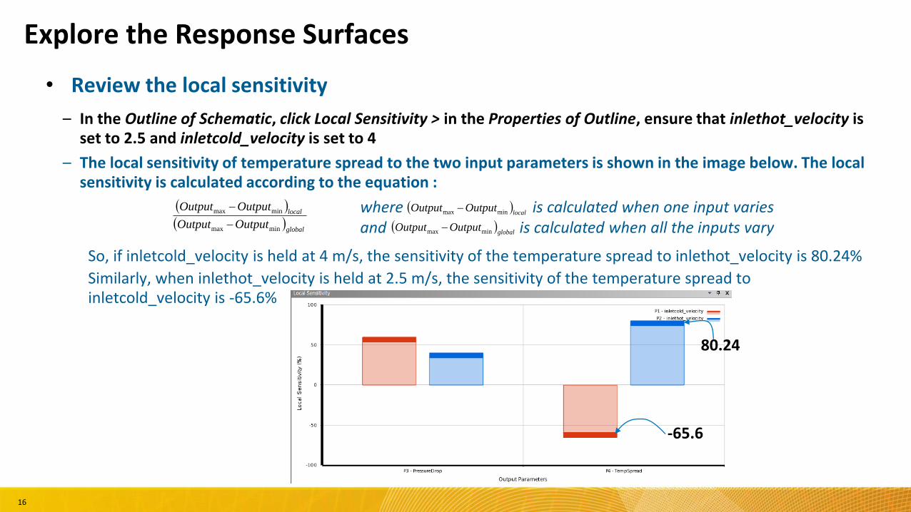
– In the Outline of Schematic, click Local Sensitivity > in the Properties of Outline, ensure that inlethot_velocity is set to 2.5 and inletcold_velocity is set to 4

– The local sensitivity of temperature spread to the two input parameters is shown in the image below. The local sensitivity is calculated according to the equation :

So, if inletcold_velocity is held at 4 m/s, the sensitivity of the temperature spread to inlethot_velocity is 80.24%

Similarly, when inlethot_velocity is held at 2.5 m/s, the sensitivity of the temperature spread to inletcold_velocity is -65.6%

80.24

-65.6

global

local

OutputOutput

OutputOutput

minmax

minmax


local

OutputOutput minmax where is calculated when one input varies and is calculated when all the inputs vary

globalOutputOutput minmax

16


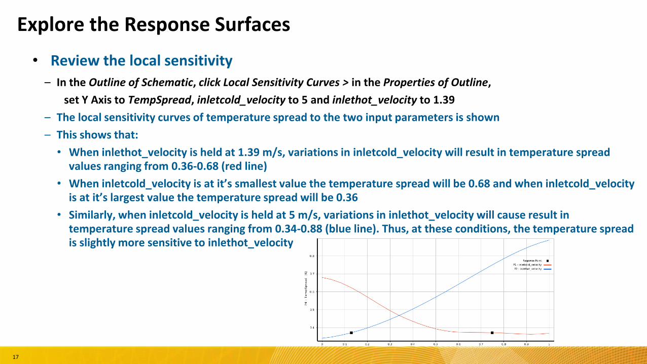
– In the Outline of Schematic, click Local Sensitivity Curves > in the Properties of Outline,

set Y Axis to TempSpread, inletcold_velocity to 5 and inlethot_velocity to 1.39

– The local sensitivity curves of temperature spread to the two input parameters is shown

– This shows that:

• When inlethot_velocity is held at 1.39 m/s, variations in inletcold_velocity will result in temperature spread values ranging from 0.36-0.68 (red line)

• When inletcold_velocity is at it’s smallest value the temperature spread will be 0.68 and when inletcold_velocity is at it’s largest value the temperature spread will be 0.36

• Similarly, when inletcold_velocity is held at 5 m/s, variations in inlethot_velocity will cause result in temperature spread values ranging from 0.34-0.88 (blue line). Thus, at these conditions, the temperature spread is slightly more sensitive to inlethot_velocity


17


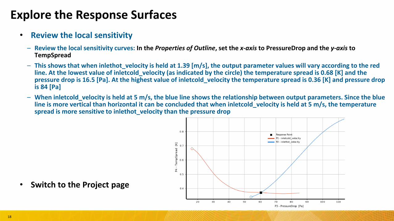
– Review the local sensitivity curves: In the Properties of Outline, set the x-axis to PressureDrop and the y-axis to TempSpread

– This shows that when inlethot_velocity is held at 1.39 [m/s], the output parameter values will vary according to the red line. At the lowest value of inletcold_velocity (as indicated by the circle) the temperature spread is 0.68 [K] and the pressure drop is 16.5 [Pa]. At the highest value of inletcold_velocity the temperature spread is 0.36 [K] and pressure drop is 84 [Pa]

– When inletcold_velocity is held at 5 m/s, the blue line shows the relationship between output parameters. Since the blue line is more vertical than horizontal it can be concluded that when inletcold_velocity is held at 5 m/s, the temperature spread is more sensitive to inlethot_velocity than the pressure drop

• Switch to the Project page


18

• Explore the Screening optimization method

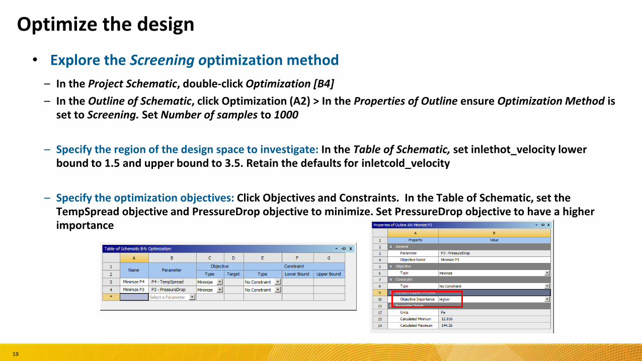
– In the Project Schematic, double-click Optimization [B4]

– In the Outline of Schematic, click Optimization (A2) > In the Properties of Outline ensure Optimization Method is set to Screening. Set Number of samples to 1000

– Specify the region of the design space to investigate: In the Table of Schematic, set inlethot_velocity lower bound to 1.5 and upper bound to 3.5. Retain the defaults for inletcold_velocity

– Specify the optimization objectives: Click Objectives and Constraints. In the Table of Schematic, set the TempSpread objective and PressureDrop objective to minimize. Set PressureDrop objective to have a higher importance

Optimize the design

19

• Explore the Screening optimization method

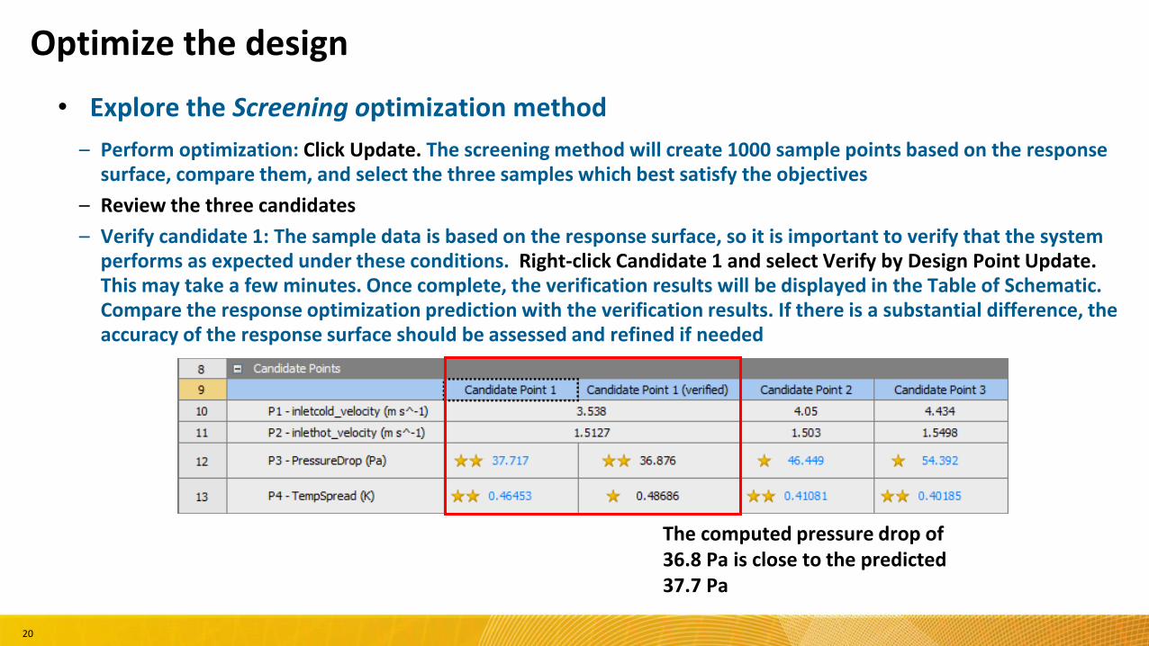
– Perform optimization: Click Update. The screening method will create 1000 sample points based on the response surface, compare them, and select the three samples which best satisfy the objectives

– Review the three candidates

– Verify candidate 1: The sample data is based on the response surface, so it is important to verify that the system performs as expected under these conditions. Right-click Candidate 1 and select Verify by Design Point Update. This may take a few minutes. Once complete, the verification results will be displayed in the Table of Schematic. Compare the response optimization prediction with the verification results. If there is a substantial difference, the accuracy of the response surface should be assessed and refined if needed

The computed pressure drop of 36.8 Pa is close to the predicted 37.7 Pa

Optimize the design

20

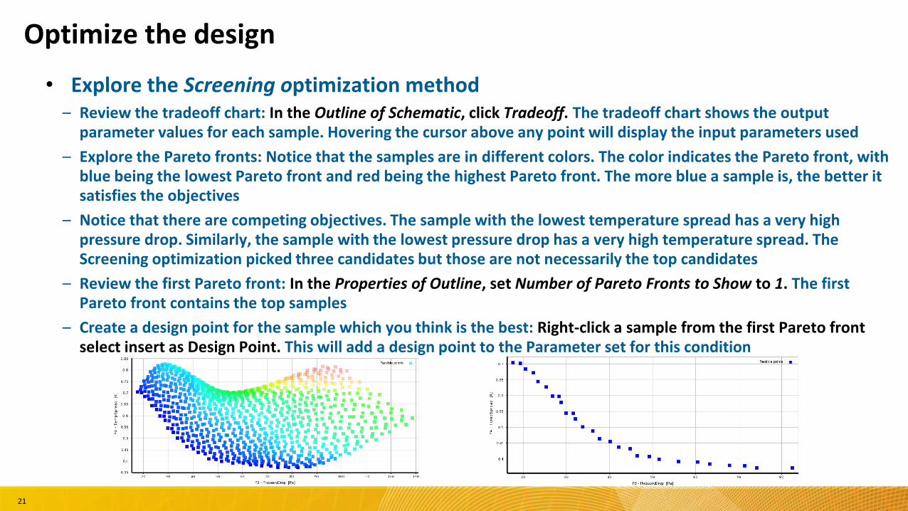
• Explore the Screening optimization method– Review the tradeoff chart: In the Outline of Schematic, click Tradeoff. The tradeoff chart shows the output

parameter values for each sample. Hovering the cursor above any point will display the input parameters used

– Explore the Pareto fronts: Notice that the samples are in different colors. The color indicates the Pareto front, with blue being the lowest Pareto front and red being the highest Pareto front. The more blue a sample is, the better it satisfies the objectives

– Notice that there are competing objectives. The sample with the lowest temperature spread has a very high pressure drop. Similarly, the sample with the lowest pressure drop has a very high temperature spread. The Screening optimization picked three candidates but those are not necessarily the top candidates

– Review the first Pareto front: In the Properties of Outline, set Number of Pareto Fronts to Show to 1. The first Pareto front contains the top samples

– Create a design point for the sample which you think is the best: Right-click a sample from the first Pareto front select insert as Design Point. This will add a design point to the Parameter set for this condition

Optimize the design

21

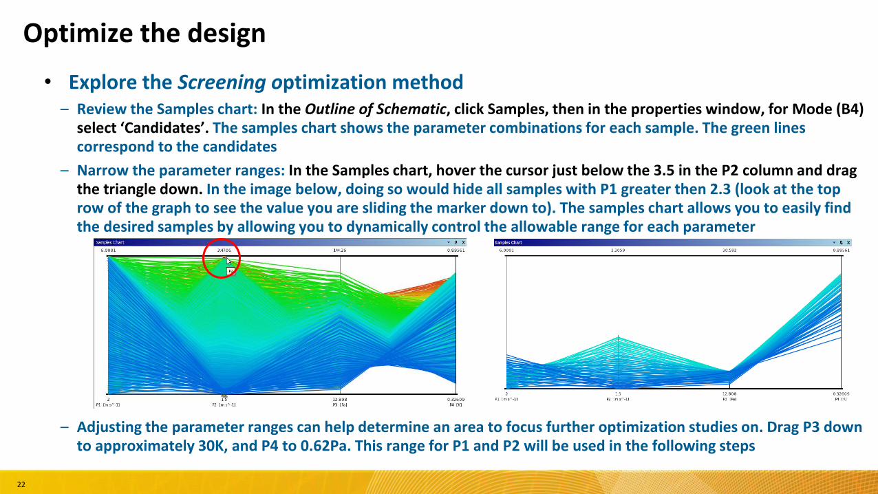
• Explore the Screening optimization method– Review the Samples chart: In the Outline of Schematic, click Samples, then in the properties window, for Mode (B4)

select ‘Candidates’. The samples chart shows the parameter combinations for each sample. The green lines correspond to the candidates

– Narrow the parameter ranges: In the Samples chart, hover the cursor just below the 3.5 in the P2 column and drag the triangle down. In the image below, doing so would hide all samples with P1 greater then 2.3 (look at the top row of the graph to see the value you are sliding the marker down to). The samples chart allows you to easily find the desired samples by allowing you to dynamically control the allowable range for each parameter

– Adjusting the parameter ranges can help determine an area to focus further optimization studies on. Drag P3 down to approximately 30K, and P4 to 0.62Pa. This range for P1 and P2 will be used in the following steps

Optimize the design

22

• Explore the MOGA optimization method

– Select the MOGA (Multi-Objective Generic Algorithm) method: In the Outline of Schematic, click Optimization (A2) > In the Properties of Outline set Optimization Method to MOGA. Review the other options related to MOGA

– Narrow the optimization domain: Select each of the 2 inlet velocities in the Outline of Schematic, then in the Table of Schematic, set the lower bound of P1 (inletcold_velocity) to 2 and the upper bound to 3.75. For P2 (inlethot_velocity), set the bounds to 1.5 and 1.8 respectively. Click Update

– Review the candidate points and other graphs, in a similar way to the previous slides (when we had used the Screening Optimizer rather than MOGA)

– The accuracy of the Screening method depends on the number of samples used. If a sample point does not exist for the optimal condition, the Screening method will not find it. For this reason the Screening method is only good at narrowing the optimization domain but not for finding the optimal condition. Instead, optimization studies should finish with MOGA or NLPQL. With the current settings, the optimizer will retain a set of 100 sample points while iterating several times, removing the worst samples and adding new ones, until 70% of the samples are in the first Pareto front or 20 iterations have been reached

Optimize the design

23

Summary:

• In this workshop you parameterized boundary conditions in FLUENT and expressions in CFD-Post, and explored the features within the DOE, Response Surface and Optimization cells. It was shown that model selection has a significant impact on results so it is good practice to always check the goodness of fit and the maximum predicted error to ensure that your model selections are appropriate. For optimization, a preliminary optimization study was done using the Screening method to narrow the optimization domain and the optimal condition was found using MOGA

Final Statements

24

Ansys Tutorial 8 Mixing Tank - drahmednagib.comdrahmednagib.com/onewebmedia/Optimum-Design-2016/Tut v 15/Tutorial_8... · Ansys Tutorial 8 Mixing Tank Optimum Design Course Fall 2016

Documents