1 ANNA UNIVERSITY OF TECHNOLOGY, TIRUCHIRAPPALLI TIRUCHIRAPPALLI-624 024 DEPARTMENT OF MECHANICAL ENGINEERING ME1404- COMPUTER AIDED SIMULATION AND ANLAYSIS LABORATORY MANUAL Prepared By Approved By PON AZHAGIRI Dr. T.SENTHIL KUMAR

Welcome message from author
This document is posted to help you gain knowledge. Please leave a comment to let me know what you think about it! Share it to your friends and learn new things together.
Transcript

1
ANNA UNIVERSITY OF TECHNOLOGY, TIRUCHIRAPPALLI
TIRUCHIRAPPALLI-624 024
DEPARTMENT OF MECHANICAL ENGINEERING
ME1404- COMPUTER AIDED SIMULATION AND ANLAYSIS
LABORATORY MANUAL
Prepared By Approved By
PON AZHAGIRI Dr. T.SENTHIL KUMAR

2
Sl.No. Date Title of the Exercise Page Number Remarks
1 Stress analysis of a plate with a circular hole.
2 Stress analysis of simple bracket.
3 Stress analysis of rectangular L bracket
4 Stress analysis of an Axisymmetric component.
5 Stress analysis of Cantilever beam.
6 Stress analysis of Simply supported beam.
7 Stress analysis of Fixed beam.
8 Mode frequency analysis of a 2 D component.
9 Mode frequency analysis of Cantilever beam.
10 Mode frequency analysis of Simply supported beam.
11 Mode frequency analysis of Fixed beam.
12 Harmonic analysis of a 2D component
13 Thermal stress analysis of a 2D component – static
14 Conductive heat transfer analysis of a 2D component
15 Convective heat transfer analysis of a 2D component
3
Ex. No. : 01 STRESS ANALYSIS OF A PLATE WITH A CIRCULAR HOLE
Date :
AIM:
To determine the displacement and bending stress of a given plate with a circular hole using Finite Element Analysis bases ANSYS structure and view the displacement and bending stress plots. PROCEDURE:
A flat rectangular plate with a hole shown in the following figure:
Preprocessing: Defining the Problem
1. Give the Simplified Version a Title
Utility Menu > File > Change Title
2. Form Geometry
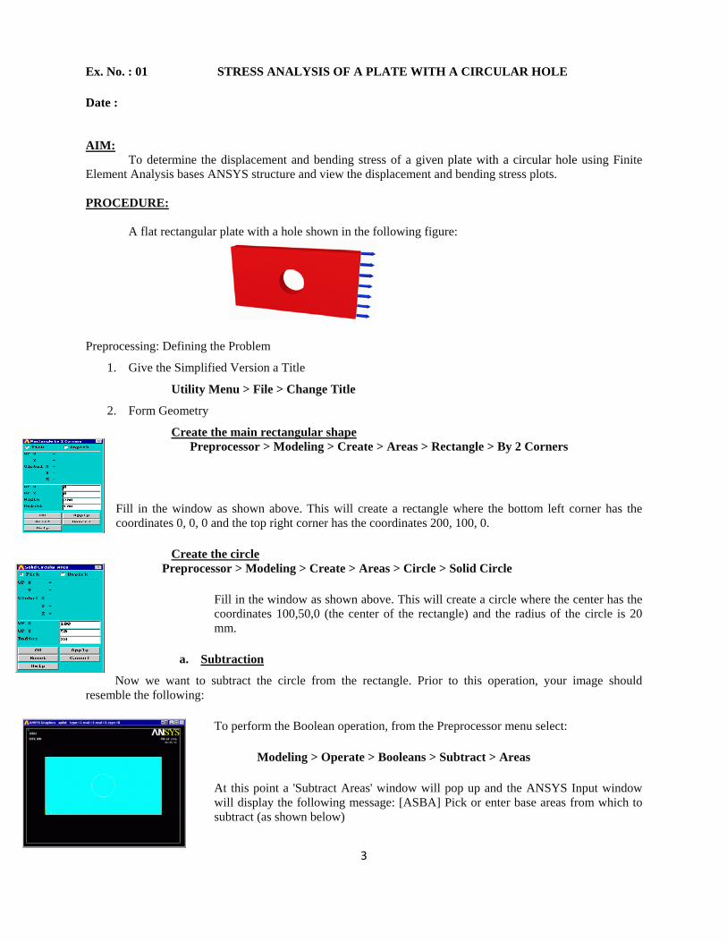
Create the main rectangular shape Preprocessor > Modeling > Create > Areas > Rectangle > By 2 Corners
Fill in the window as shown above. This will create a rectangle where the bottom left corner has the coordinates 0, 0, 0 and the top right corner has the coordinates 200, 100, 0.
Create the circle Preprocessor > Modeling > Create > Areas > Circle > Solid Circle
Fill in the window as shown above. This will create a circle where the center has the coordinates 100,50,0 (the center of the rectangle) and the radius of the circle is 20 mm.
a. Subtraction
Now we want to subtract the circle from the rectangle. Prior to this operation, your image should resemble the following:
To perform the Boolean operation, from the Preprocessor menu select:
Modeling > Operate > Booleans > Subtract > Areas
At this point a 'Subtract Areas' window will pop up and the ANSYS Input window will display the following message: [ASBA] Pick or enter base areas from which to subtract (as shown below)
4
Therefore, select the base area (the rectangle) by clicking on it. Note: The selected area will turn pink once it is selected.
The following window may appear because there are 2 areas at the location you clicked.
Ensure that the entire rectangular area is selected (otherwise click 'Next') and then click 'OK'.
Click 'OK' on the 'Subtract Areas' window.
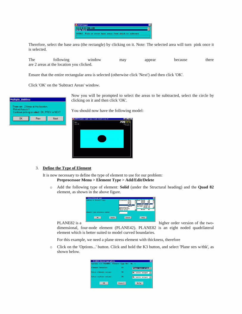
Now you will be prompted to select the areas to be subtracted, select the circle by clicking on it and then click 'OK'.
You should now have the following model:
3. Define the Type of Element
It is now necessary to define the type of element to use for our problem: Preprocessor Menu > Element Type > Add/Edit/Delete
o Add the following type of element: Solid (under the Structural heading) and the Quad 82 element, as shown in the above figure.
PLANE82 is a higher order version of the two-dimensional, four-node element (PLANE42). PLANE82 is an eight noded quadrilateral element which is better suited to model curved boundaries.
For this example, we need a plane stress element with thickness, therefore
o Click on the 'Options...' button. Click and hold the K3 button, and select 'Plane strs w/thk', as shown below.
5
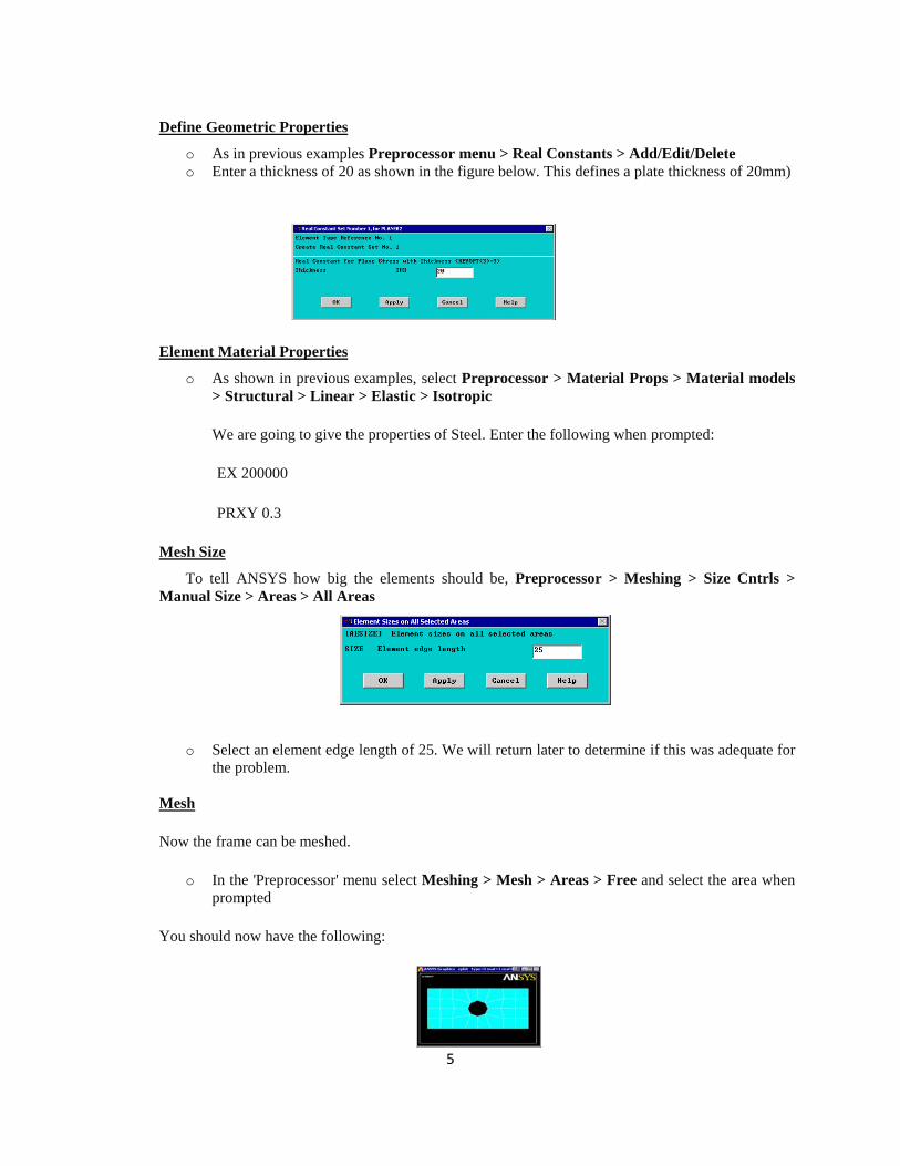
Define Geometric Properties
o As in previous examples Preprocessor menu > Real Constants > Add/Edit/Delete o Enter a thickness of 20 as shown in the figure below. This defines a plate thickness of 20mm)
Element Material Properties
o As shown in previous examples, select Preprocessor > Material Props > Material models > Structural > Linear > Elastic > Isotropic
We are going to give the properties of Steel. Enter the following when prompted:
EX 200000
PRXY 0.3
Mesh Size
To tell ANSYS how big the elements should be, Preprocessor > Meshing > Size Cntrls > Manual Size > Areas > All Areas
o Select an element edge length of 25. We will return later to determine if this was adequate for the problem.
Mesh
Now the frame can be meshed.
o In the 'Preprocessor' menu select Meshing > Mesh > Areas > Free and select the area when prompted
You should now have the following:
6
Solution Phase: Assigning Loads and Solving
You have now defined your model. It is now time to apply the load(s) and constraint(s) and solve the resulting system of equations.
1. Define Analysis Type o Ensure that a Static Analysis will be performed (Solution > Analysis Type > New Analysis).
2. Apply Constraints
As shown previously, the left end of the plate is fixed.
o In the Solution > Define Loads > Apply > Structural > Displacement > On Lines
o Select the left end of the plate and click on 'Apply' in the 'Apply U,ROT on Lines' window.
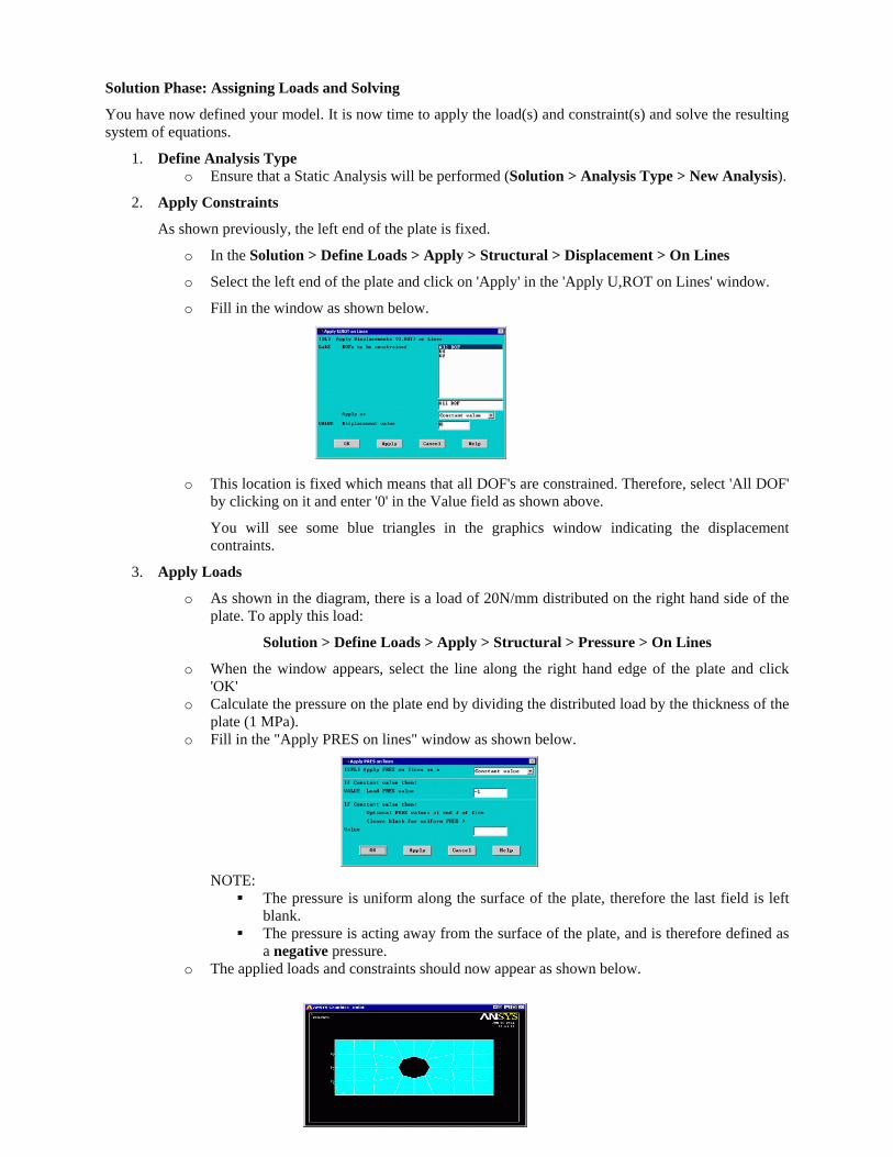
o Fill in the window as shown below.
o This location is fixed which means that all DOF's are constrained. Therefore, select 'All DOF' by clicking on it and enter '0' in the Value field as shown above.
You will see some blue triangles in the graphics window indicating the displacement contraints.
3. Apply Loads
o As shown in the diagram, there is a load of 20N/mm distributed on the right hand side of the plate. To apply this load:
Solution > Define Loads > Apply > Structural > Pressure > On Lines
o When the window appears, select the line along the right hand edge of the plate and click 'OK'
o Calculate the pressure on the plate end by dividing the distributed load by the thickness of the plate (1 MPa).
o Fill in the "Apply PRES on lines" window as shown below. NOTE:
The pressure is uniform along the surface of the plate, therefore the last field is left blank.
The pressure is acting away from the surface of the plate, and is therefore defined as a negative pressure.
o The applied loads and constraints should now appear as shown below.
7
4. Solving the System
Solution > Solve > Current LS
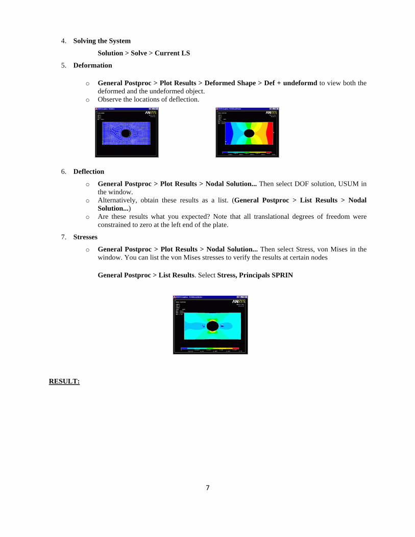
5. Deformation
o General Postproc > Plot Results > Deformed Shape > Def + undeformd to view both the deformed and the undeformed object.
o Observe the locations of deflection.
6. Deflection
o General Postproc > Plot Results > Nodal Solution... Then select DOF solution, USUM in the window.
o Alternatively, obtain these results as a list. (General Postproc > List Results > Nodal Solution...)
o Are these results what you expected? Note that all translational degrees of freedom were constrained to zero at the left end of the plate.
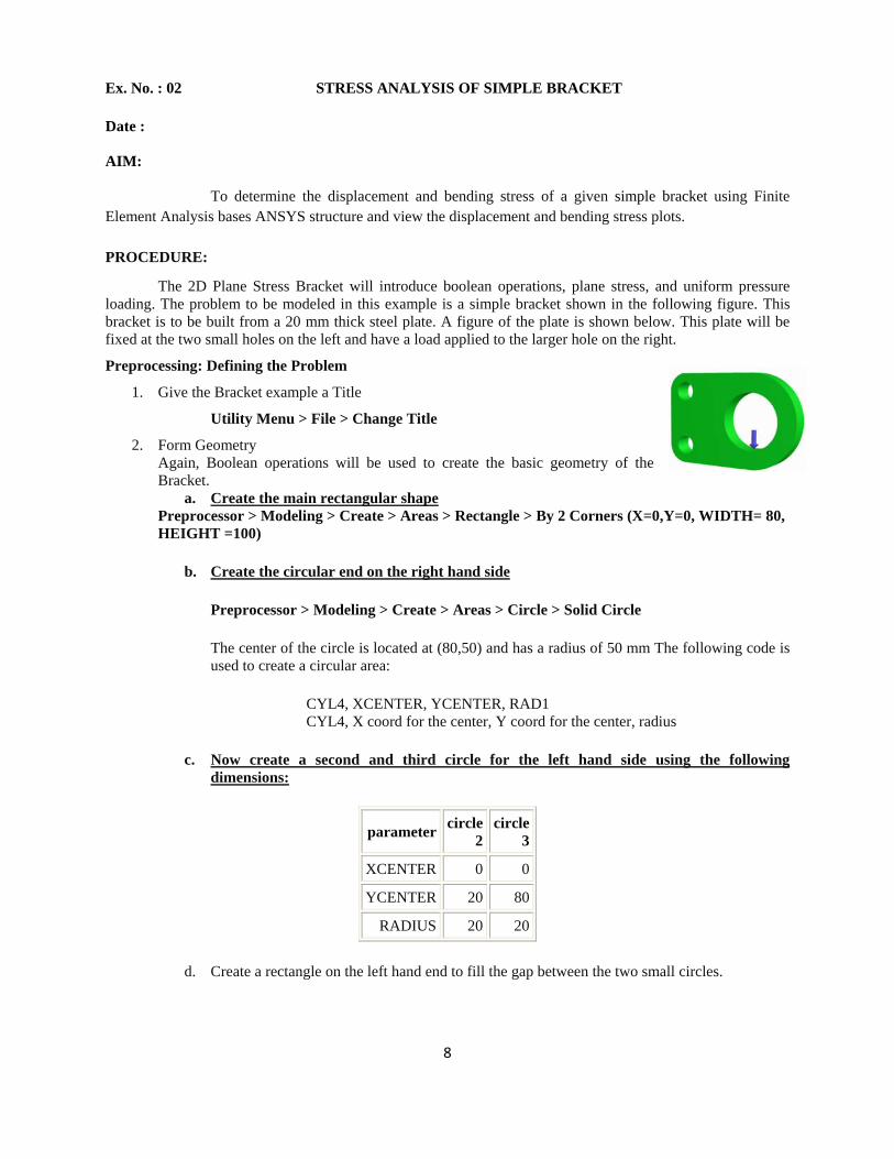
7. Stresses
o General Postproc > Plot Results > Nodal Solution... Then select Stress, von Mises in the window. You can list the von Mises stresses to verify the results at certain nodes
General Postproc > List Results. Select Stress, Principals SPRIN
RESULT:
8
Ex. No. : 02 STRESS ANALYSIS OF SIMPLE BRACKET
Date :
AIM:
To determine the displacement and bending stress of a given simple bracket using Finite Element Analysis bases ANSYS structure and view the displacement and bending stress plots.
PROCEDURE:
The 2D Plane Stress Bracket will introduce boolean operations, plane stress, and uniform pressure loading. The problem to be modeled in this example is a simple bracket shown in the following figure. This bracket is to be built from a 20 mm thick steel plate. A figure of the plate is shown below. This plate will be fixed at the two small holes on the left and have a load applied to the larger hole on the right.
Preprocessing: Defining the Problem
1. Give the Bracket example a Title
Utility Menu > File > Change Title
2. Form Geometry Again, Boolean operations will be used to create the basic geometry of the Bracket.
a. Create the main rectangular shape Preprocessor > Modeling > Create > Areas > Rectangle > By 2 Corners (X=0,Y=0, WIDTH= 80, HEIGHT =100)
b. Create the circular end on the right hand side
Preprocessor > Modeling > Create > Areas > Circle > Solid Circle
The center of the circle is located at (80,50) and has a radius of 50 mm The following code is used to create a circular area:
CYL4, XCENTER, YCENTER, RAD1 CYL4, X coord for the center, Y coord for the center, radius
c. Now create a second and third circle for the left hand side using the following dimensions:
parameter circle 2
circle 3
XCENTER 0 0
YCENTER 20 80
RADIUS 20 20
d. Create a rectangle on the left hand end to fill the gap between the two small circles.
9
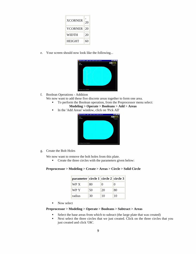
e. Your screen should now look like the following...
f. Boolean Operations - Addition We now want to add these five discrete areas together to form one area.
To perform the Boolean operation, from the Preprocessor menu select: Modeling > Operate > Booleans > Add > Areas
In the 'Add Areas' window, click on 'Pick All'
g. Create the Bolt Holes
We now want to remove the bolt holes from this plate. Create the three circles with the parameters given below:
Preprocessor > Modeling > Create > Areas > Circle > Solid Circle
parameter circle 1 circle 2 circle 3
WP X 80 0 0
WP Y 50 20 80
radius 30 10 10
Now select
Preprocessor > Modeling > Operate > Booleans > Subtract > Areas
Select the base areas from which to subract (the large plate that was created) Next select the three circles that we just created. Click on the three circles that you
just created and click 'OK'.
XCORNER -20
YCORNER 20
WIDTH 20
HEIGHT 60

10
Now you should have the following:
3. Define the Type of Element
As in the verification model, PLANE82 will be used for this example
o Preprocessor > Element Type > Add/Edit/Delete
o Use the 'Options...' button to get a plane stress element with thickness
o Under the Extra Element Output K5 select nodal stress.
Define Geometric Contants
o Preprocessor > Real Constants > Add/Edit/Delete o Enter a thickness of 20mm.
Element Material Properties
o Preprocessor > Material Props > Material Library > Structural > Linear > Elastic > Isotropic We are going to give the properties of Steel. Enter the following when prompted:
EX 200000 PRXY 0.3
Mesh Size
o Preprocessor > Meshing > Size Cntrls > Manual Size > Areas > All Areas o Select an element edge length of 5. Again, we will need to make sure the model has
converged.
Mesh
Preprocessor > Meshing > Mesh > Areas > Free and select the area when prompted
Solution Phase: Assigning Loads and Solving
You have now defined your model. It is now time to apply the load(s) and constraint(s) and solve the the resulting system of equations.
1. Define Analysis Type
o 'Solution' > 'New Analysis' and select 'Static'.
2. Apply Constraints
11
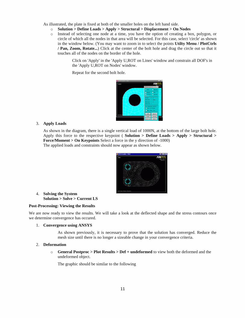
As illustrated, the plate is fixed at both of the smaller holes on the left hand side. o Solution > Define Loads > Apply > Structural > Displacement > On Nodes o Instead of selecting one node at a time, you have the option of creating a box, polygon, or
circle of which all the nodes in that area will be selected. For this case, select 'circle' as shown in the window below. (You may want to zoom in to select the points Utilty Menu / PlotCtrls / Pan, Zoom, Rotate...) Click at the center of the bolt hole and drag the circle out so that it touches all of the nodes on the border of the hole.
Click on 'Apply' in the 'Apply U,ROT on Lines' window and constrain all DOF's in the 'Apply U,ROT on Nodes' window.
Repeat for the second bolt hole.
3. Apply Loads
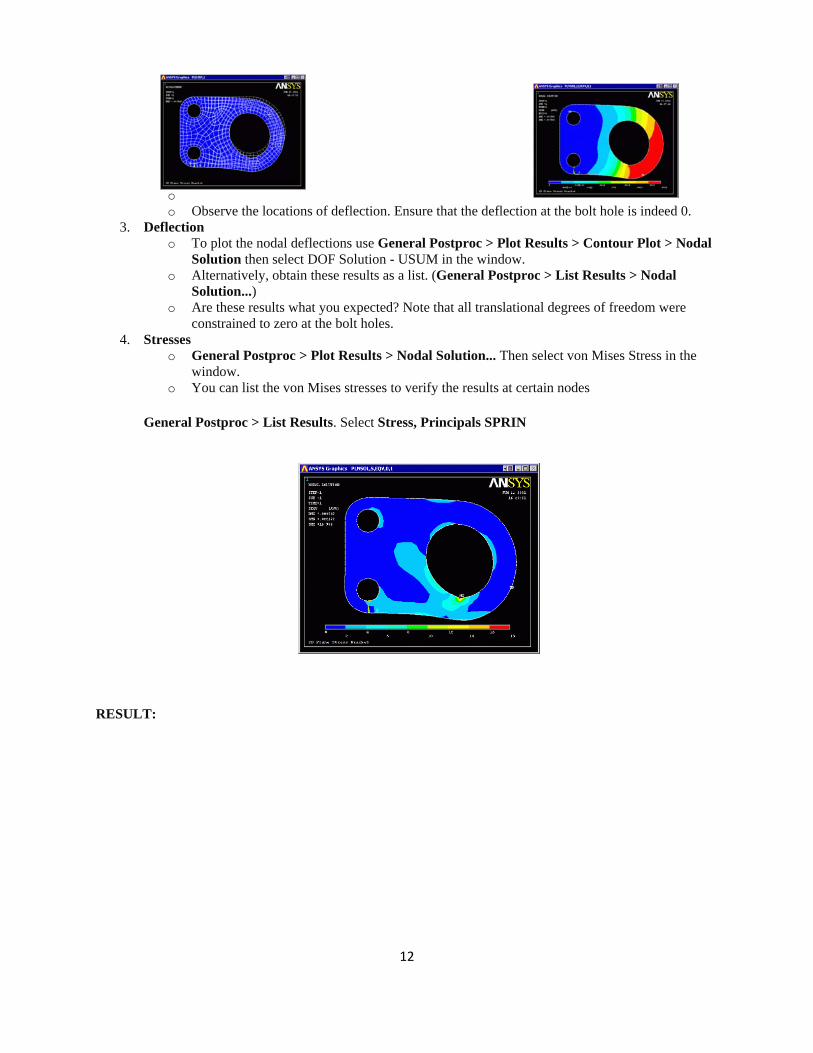
As shown in the diagram, there is a single vertical load of 1000N, at the bottom of the large bolt hole. Apply this force to the respective keypoint ( Solution > Define Loads > Apply > Structural > Force/Moment > On Keypoints Select a force in the y direction of -1000) The applied loads and constraints should now appear as shown below.
4. Solving the System Solution > Solve > Current LS
Post-Processing: Viewing the Results
We are now ready to view the results. We will take a look at the deflected shape and the stress contours once we determine convergence has occured.
1. Convergence using ANSYS
As shown previously, it is necessary to prove that the solution has converged. Reduce the mesh size until there is no longer a sizeable change in your convergence criteria.
2. Deformation
o General Postproc > Plot Results > Def + undeformed to view both the deformed and the undeformed object.
The graphic should be similar to the following
12
o o o o o o o Observe the locations of deflection. Ensure that the deflection at the bolt hole is indeed 0.
3. Deflection o To plot the nodal deflections use General Postproc > Plot Results > Contour Plot > Nodal
Solution then select DOF Solution - USUM in the window. o Alternatively, obtain these results as a list. (General Postproc > List Results > Nodal
Solution...) o Are these results what you expected? Note that all translational degrees of freedom were
constrained to zero at the bolt holes. 4. Stresses
o General Postproc > Plot Results > Nodal Solution... Then select von Mises Stress in the window.
o You can list the von Mises stresses to verify the results at certain nodes
General Postproc > List Results. Select Stress, Principals SPRIN
RESULT:
13
Ex. No. : 03. STRESS ANALYSIS OF RECTANGULAR L - BRACKET
Date :
AIM:
To determine the displacement and bending stress of a given L - bracket using Finite Element Analysis bases ANSYS structure and view the displacement and bending stress plots.
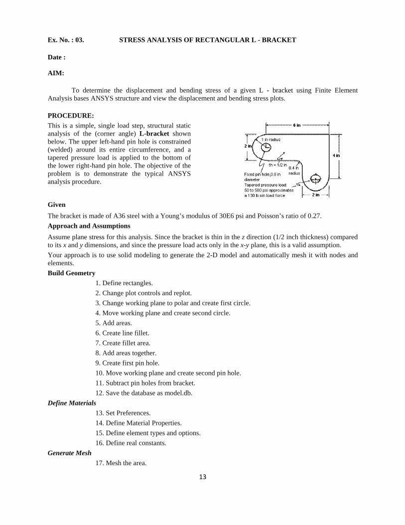
PROCEDURE: This is a simple, single load step, structural static analysis of the (corner angle) L-bracket shown below. The upper left-hand pin hole is constrained (welded) around its entire circumference, and a tapered pressure load is applied to the bottom of the lower right-hand pin hole. The objective of the problem is to demonstrate the typical ANSYS analysis procedure.
Given The bracket is made of A36 steel with a Young’s modulus of 30E6 psi and Poisson’s ratio of 0.27. Approach and Assumptions Assume plane stress for this analysis. Since the bracket is thin in the z direction (1/2 inch thickness) compared to its x and y dimensions, and since the pressure load acts only in the x-y plane, this is a valid assumption. Your approach is to use solid modeling to generate the 2-D model and automatically mesh it with nodes and elements. Build Geometry
1. Define rectangles. 2. Change plot controls and replot. 3. Change working plane to polar and create first circle. 4. Move working plane and create second circle. 5. Add areas. 6. Create line fillet. 7. Create fillet area. 8. Add areas together. 9. Create first pin hole. 10. Move working plane and create second pin hole. 11. Subtract pin holes from bracket. 12. Save the database as model.db.
Define Materials 13. Set Preferences. 14. Define Material Properties. 15. Define element types and options. 16. Define real constants.
Generate Mesh 17. Mesh the area.
14
Apply Loads 19. Apply displacement constraints. 20. Apply pressure load.
Obtain Solution 21. Solve.
Review Results 22. Enter the general postprocessor and read in the results. 23. Plot the deformed shape. 24. Plot the von Mises equivalent stress. 25. List the reaction solution.
Step 1: Define rectangles. There are several ways to create the model geometry within ANSYS, some more convenient than others. The first step is to recognize that you can construct the bracket easily with combinations of rectangles and circle Primitives. Decide where the origin will be located and then define the rectangle and circle primitives relative to that origin. The location of the origin is arbitrary. Here, use the center of the upper left-hand hole. ANSYS does not need to know where the origin is. Simply begin by defining a rectangle relative to that location. In ANSYS, this origin is called the global origin.
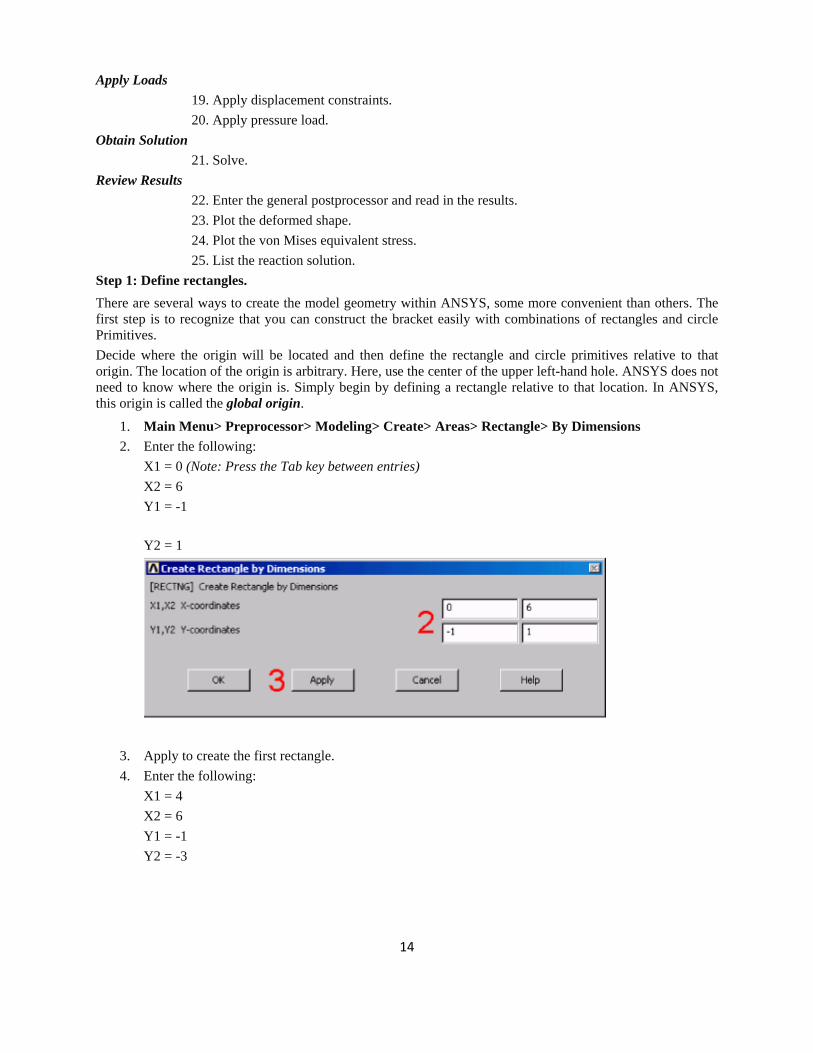
1. Main Menu> Preprocessor> Modeling> Create> Areas> Rectangle> By Dimensions 2. Enter the following:
X1 = 0 (Note: Press the Tab key between entries) X2 = 6 Y1 = -1
Y2 = 1
3. Apply to create the first rectangle. 4. Enter the following:
X1 = 4 X2 = 6 Y1 = -1 Y2 = -3
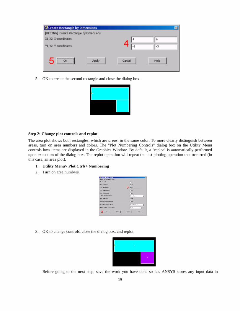
15
5. OK to create the second rectangle and close the dialog box.
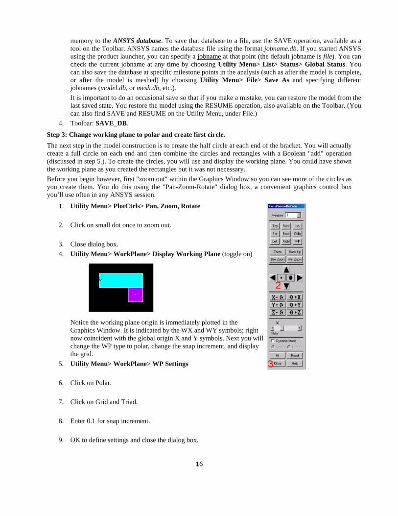
Step 2: Change plot controls and replot. The area plot shows both rectangles, which are areas, in the same color. To more clearly distinguish between areas, turn on area numbers and colors. The "Plot Numbering Controls" dialog box on the Utility Menu controls how items are displayed in the Graphics Window. By default, a "replot" is automatically performed upon execution of the dialog box. The replot operation will repeat the last plotting operation that occurred (in this case, an area plot).
1. Utility Menu> Plot Ctrls> Numbering 2. Turn on area numbers.
3. OK to change controls, close the dialog box, and replot.
Before going to the next step, save the work you have done so far. ANSYS stores any input data in
16
memory to the ANSYS database. To save that database to a file, use the SAVE operation, available as a tool on the Toolbar. ANSYS names the database file using the format jobname.db. If you started ANSYS using the product launcher, you can specify a jobname at that point (the default jobname is file). You can check the current jobname at any time by choosing Utility Menu> List> Status> Global Status. You can also save the database at specific milestone points in the analysis (such as after the model is complete, or after the model is meshed) by choosing Utility Menu> File> Save As and specifying different jobnames (model.db, or mesh.db, etc.). It is important to do an occasional save so that if you make a mistake, you can restore the model from the last saved state. You restore the model using the RESUME operation, also available on the Toolbar. (You can also find SAVE and RESUME on the Utility Menu, under File.)
4. Toolbar: SAVE_DB.
Step 3: Change working plane to polar and create first circle. The next step in the model construction is to create the half circle at each end of the bracket. You will actually create a full circle on each end and then combine the circles and rectangles with a Boolean "add" operation (discussed in step 5.). To create the circles, you will use and display the working plane. You could have shown the working plane as you created the rectangles but it was not necessary. Before you begin however, first "zoom out" within the Graphics Window so you can see more of the circles as you create them. You do this using the "Pan-Zoom-Rotate" dialog box, a convenient graphics control box you’ll use often in any ANSYS session.
1. Utility Menu> PlotCtrls> Pan, Zoom, Rotate
2. Click on small dot once to zoom out.
3. Close dialog box. 4. Utility Menu> WorkPlane> Display Working Plane (toggle on)
Notice the working plane origin is immediately plotted in the Graphics Window. It is indicated by the WX and WY symbols; right now coincident with the global origin X and Y symbols. Next you will change the WP type to polar, change the snap increment, and display the grid.
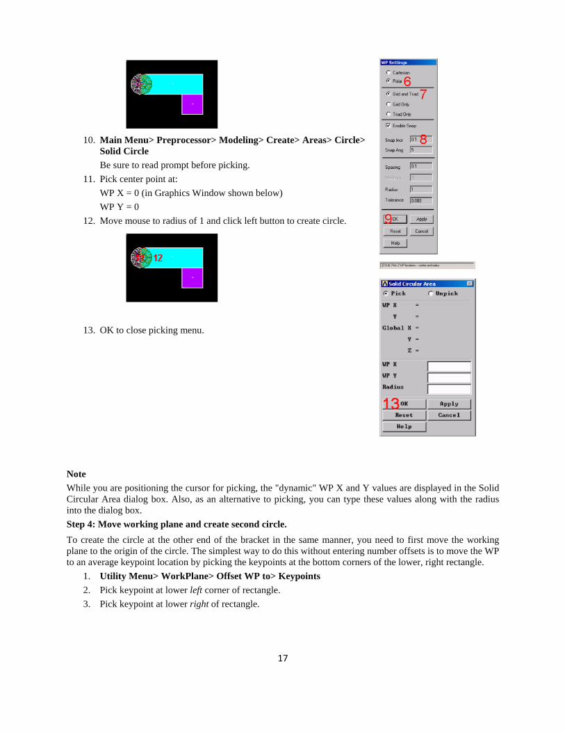
5. Utility Menu> WorkPlane> WP Settings
6. Click on Polar.
7. Click on Grid and Triad.
8. Enter 0.1 for snap increment.
9. OK to define settings and close the dialog box.
17
10. Main Menu> Preprocessor> Modeling> Create> Areas> Circle>
Solid Circle Be sure to read prompt before picking.
11. Pick center point at: WP X = 0 (in Graphics Window shown below) WP Y = 0
12. Move mouse to radius of 1 and click left button to create circle.
13. OK to close picking menu.
Note While you are positioning the cursor for picking, the "dynamic" WP X and Y values are displayed in the Solid Circular Area dialog box. Also, as an alternative to picking, you can type these values along with the radius into the dialog box. Step 4: Move working plane and create second circle. To create the circle at the other end of the bracket in the same manner, you need to first move the working plane to the origin of the circle. The simplest way to do this without entering number offsets is to move the WP to an average keypoint location by picking the keypoints at the bottom corners of the lower, right rectangle.
1. Utility Menu> WorkPlane> Offset WP to> Keypoints 2. Pick keypoint at lower left corner of rectangle. 3. Pick keypoint at lower right of rectangle.
18
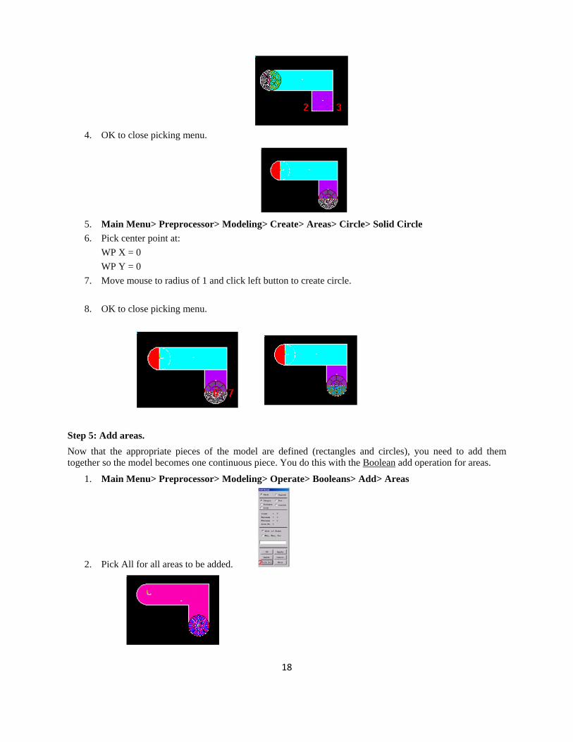
4. OK to close picking menu.
5. Main Menu> Preprocessor> Modeling> Create> Areas> Circle> Solid Circle 6. Pick center point at:
WP X = 0 WP Y = 0
7. Move mouse to radius of 1 and click left button to create circle.
8. OK to close picking menu.
Step 5: Add areas. Now that the appropriate pieces of the model are defined (rectangles and circles), you need to add them together so the model becomes one continuous piece. You do this with the Boolean add operation for areas.
1. Main Menu> Preprocessor> Modeling> Operate> Booleans> Add> Areas
2. Pick All for all areas to be added.
19
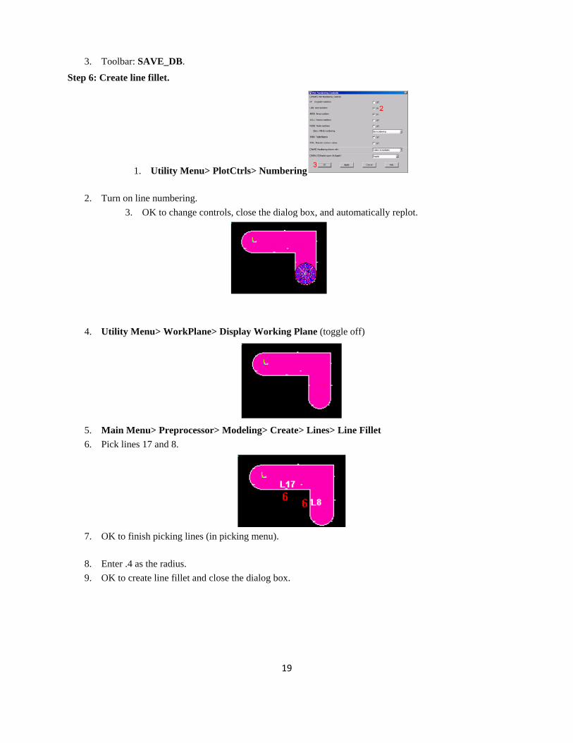
3. Toolbar: SAVE_DB.
Step 6: Create line fillet.
1. Utility Menu> PlotCtrls> Numbering
2. Turn on line numbering. 3. OK to change controls, close the dialog box, and automatically replot.
4. Utility Menu> WorkPlane> Display Working Plane (toggle off)
5. Main Menu> Preprocessor> Modeling> Create> Lines> Line Fillet 6. Pick lines 17 and 8.
7. OK to finish picking lines (in picking menu).
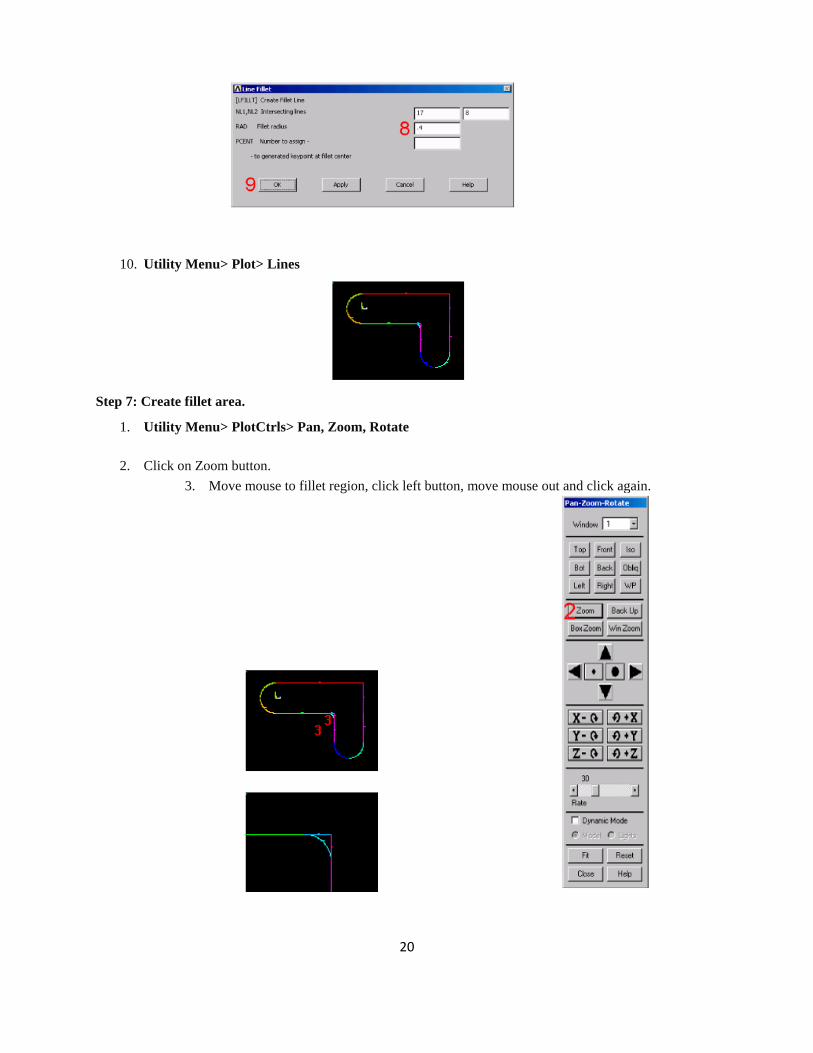
8. Enter .4 as the radius. 9. OK to create line fillet and close the dialog box.
20
10. Utility Menu> Plot> Lines
Step 7: Create fillet area.
1. Utility Menu> PlotCtrls> Pan, Zoom, Rotate
2. Click on Zoom button. 3. Move mouse to fillet region, click left button, move mouse out and click again.
21
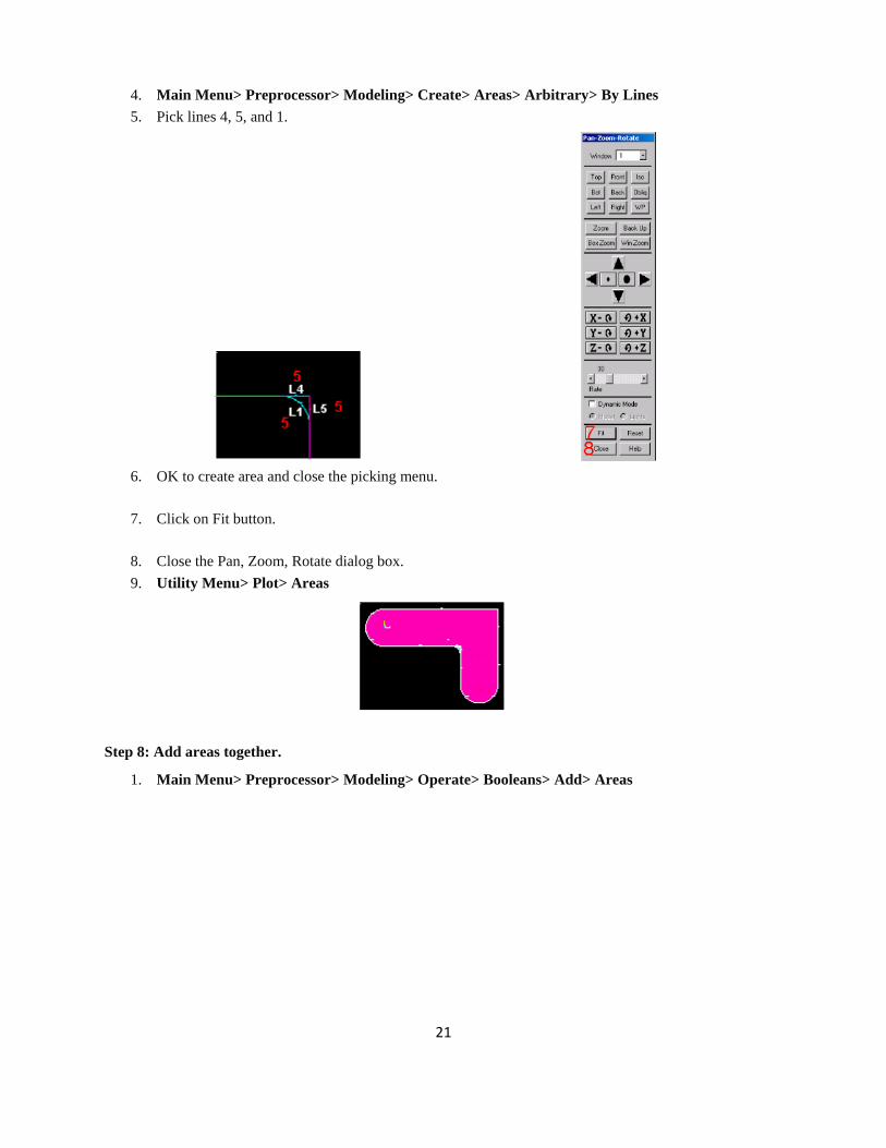
4. Main Menu> Preprocessor> Modeling> Create> Areas> Arbitrary> By Lines 5. Pick lines 4, 5, and 1.
6. OK to create area and close the picking menu.
7. Click on Fit button.
8. Close the Pan, Zoom, Rotate dialog box. 9. Utility Menu> Plot> Areas
Step 8: Add areas together.
1. Main Menu> Preprocessor> Modeling> Operate> Booleans> Add> Areas
22
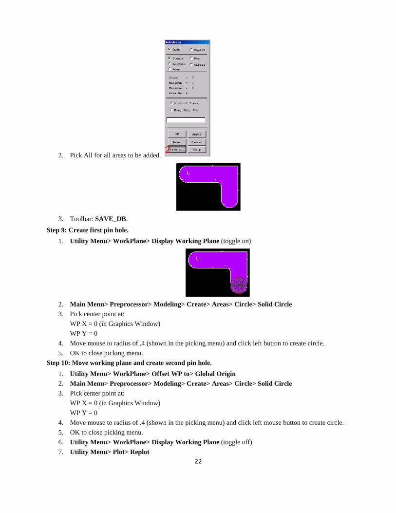
2. Pick All for all areas to be added.
3. Toolbar: SAVE_DB.
Step 9: Create first pin hole. 1. Utility Menu> WorkPlane> Display Working Plane (toggle on)
2. Main Menu> Preprocessor> Modeling> Create> Areas> Circle> Solid Circle 3. Pick center point at:
WP X = 0 (in Graphics Window) WP Y = 0
4. Move mouse to radius of .4 (shown in the picking menu) and click left button to create circle. 5. OK to close picking menu.
Step 10: Move working plane and create second pin hole. 1. Utility Menu> WorkPlane> Offset WP to> Global Origin 2. Main Menu> Preprocessor> Modeling> Create> Areas> Circle> Solid Circle 3. Pick center point at:
WP X = 0 (in Graphics Window) WP Y = 0
4. Move mouse to radius of .4 (shown in the picking menu) and click left mouse button to create circle. 5. OK to close picking menu. 6. Utility Menu> WorkPlane> Display Working Plane (toggle off) 7. Utility Menu> Plot> Replot
23
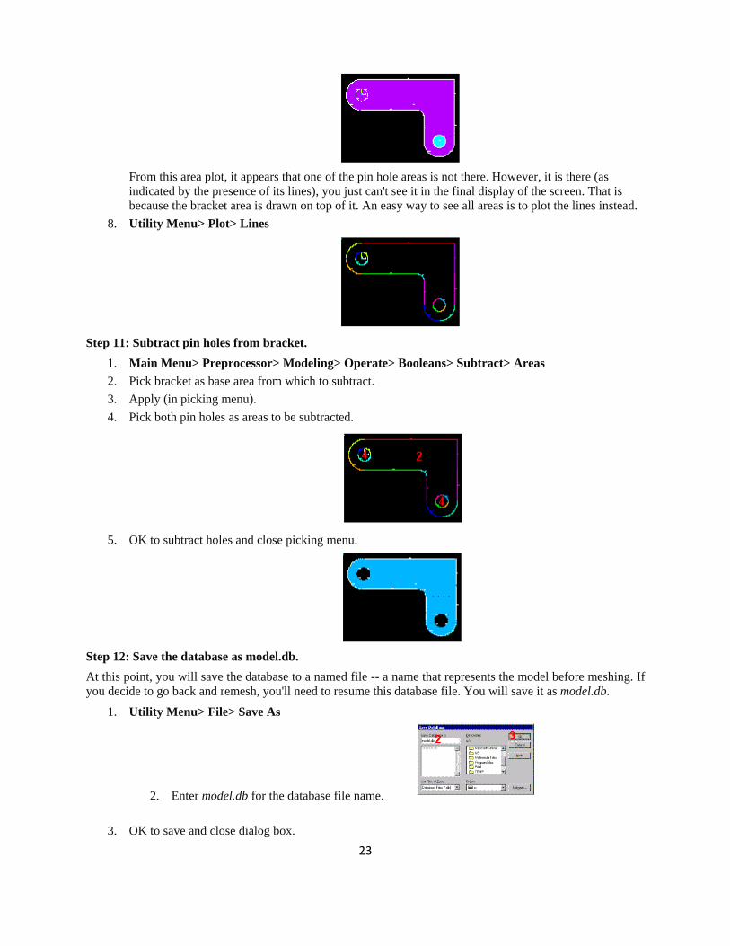
From this area plot, it appears that one of the pin hole areas is not there. However, it is there (as indicated by the presence of its lines), you just can't see it in the final display of the screen. That is because the bracket area is drawn on top of it. An easy way to see all areas is to plot the lines instead.
8. Utility Menu> Plot> Lines
Step 11: Subtract pin holes from bracket.
1. Main Menu> Preprocessor> Modeling> Operate> Booleans> Subtract> Areas 2. Pick bracket as base area from which to subtract. 3. Apply (in picking menu). 4. Pick both pin holes as areas to be subtracted.
5. OK to subtract holes and close picking menu.
Step 12: Save the database as model.db. At this point, you will save the database to a named file -- a name that represents the model before meshing. If you decide to go back and remesh, you'll need to resume this database file. You will save it as model.db.
1. Utility Menu> File> Save As
2. Enter model.db for the database file name.
3. OK to save and close dialog box.
24
Define Materials Step 13: Set preferences. In preparation for defining materials, you will set preferences so that only materials that pertain to a structural analysis are available for you to choose. To set preferences:
1. Main Menu> Preferences 2. Turn on structural filtering. The options may differ from what is shown here since they
depend on the ANSYS product you are using.
3. OK to apply filtering and close the dialog box.
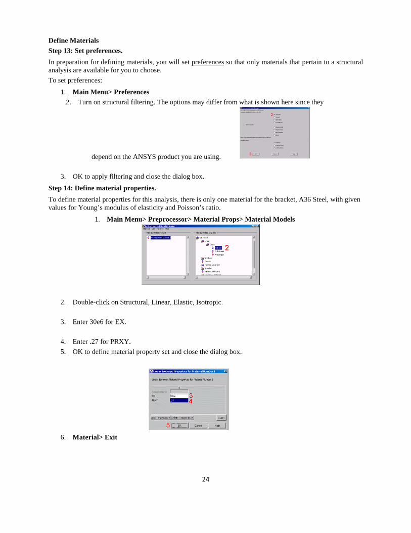
Step 14: Define material properties. To define material properties for this analysis, there is only one material for the bracket, A36 Steel, with given values for Young’s modulus of elasticity and Poisson’s ratio.
1. Main Menu> Preprocessor> Material Props> Material Models
2. Double-click on Structural, Linear, Elastic, Isotropic.
3. Enter 30e6 for EX.
4. Enter .27 for PRXY. 5. OK to define material property set and close the dialog box.
6. Material> Exit
25
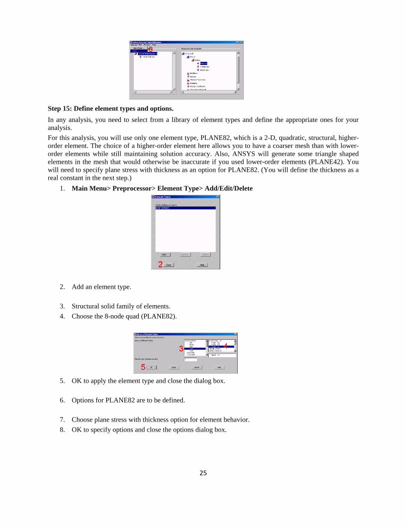
Step 15: Define element types and options. In any analysis, you need to select from a library of element types and define the appropriate ones for your analysis. For this analysis, you will use only one element type, PLANE82, which is a 2-D, quadratic, structural, higher-order element. The choice of a higher-order element here allows you to have a coarser mesh than with lower-order elements while still maintaining solution accuracy. Also, ANSYS will generate some triangle shaped elements in the mesh that would otherwise be inaccurate if you used lower-order elements (PLANE42). You will need to specify plane stress with thickness as an option for PLANE82. (You will define the thickness as a real constant in the next step.)
1. Main Menu> Preprocessor> Element Type> Add/Edit/Delete
2. Add an element type.
3. Structural solid family of elements. 4. Choose the 8-node quad (PLANE82).
5. OK to apply the element type and close the dialog box.
6. Options for PLANE82 are to be defined.
7. Choose plane stress with thickness option for element behavior. 8. OK to specify options and close the options dialog box.
26
9. Close the element type dialog box.
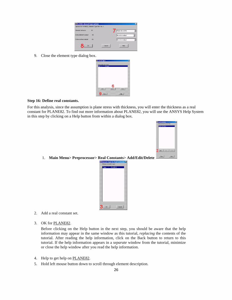
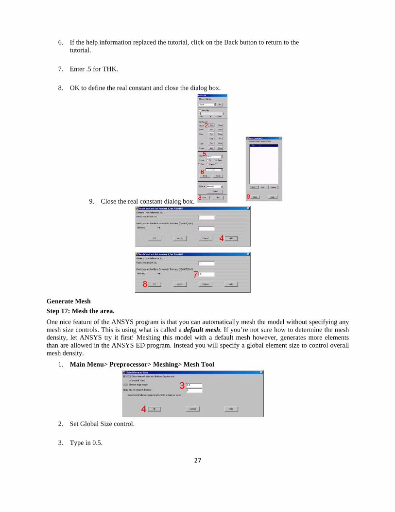
Step 16: Define real constants. For this analysis, since the assumption is plane stress with thickness, you will enter the thickness as a real constant for PLANE82. To find out more information about PLANE82, you will use the ANSYS Help System in this step by clicking on a Help button from within a dialog box.
1. Main Menu> Preprocessor> Real Constants> Add/Edit/Delete
2. Add a real constant set.
3. OK for PLANE82. Before clicking on the Help button in the next step, you should be aware that the help information may appear in the same window as this tutorial, replacing the contents of the tutorial. After reading the help information, click on the Back button to return to this tutorial. If the help information appears in a separate window from the tutorial, minimize or close the help window after you read the help information.
4. Help to get help on PLANE82. 5. Hold left mouse button down to scroll through element description.
27
6. If the help information replaced the tutorial, click on the Back button to return to the tutorial.
7. Enter .5 for THK.
8. OK to define the real constant and close the dialog box.
9. Close the real constant dialog box.
Generate Mesh Step 17: Mesh the area. One nice feature of the ANSYS program is that you can automatically mesh the model without specifying any mesh size controls. This is using what is called a default mesh. If you’re not sure how to determine the mesh density, let ANSYS try it first! Meshing this model with a default mesh however, generates more elements than are allowed in the ANSYS ED program. Instead you will specify a global element size to control overall mesh density.
1. Main Menu> Preprocessor> Meshing> Mesh Tool
2. Set Global Size control.
3. Type in 0.5.
28
4. OK.
5. Choose Area Meshing.
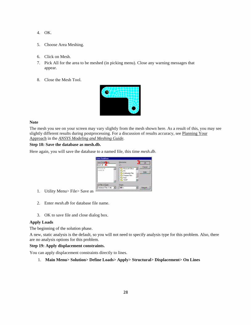
6. Click on Mesh. 7. Pick All for the area to be meshed (in picking menu). Close any warning messages that
appear.
8. Close the Mesh Tool.
Note The mesh you see on your screen may vary slightly from the mesh shown here. As a result of this, you may see slightly different results during postprocessing. For a discussion of results accuracy, see Planning Your Approach in the ANSYS Modeling and Meshing Guide. Step 18: Save the database as mesh.db. Here again, you will save the database to a named file, this time mesh.db.
1. Utility Menu> File> Save as
2. Enter mesh.db for database file name.
3. OK to save file and close dialog box.
Apply Loads The beginning of the solution phase. A new, static analysis is the default, so you will not need to specify analysis type for this problem. Also, there are no analysis options for this problem. Step 19: Apply displacement constraints. You can apply displacement constraints directly to lines.
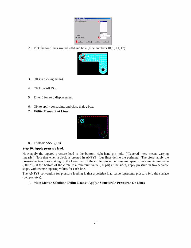
1. Main Menu> Solution> Define Loads> Apply> Structural> Displacement> On Lines
29
2. Pick the four lines around left-hand hole (Line numbers 10, 9, 11, 12).
3. OK (in picking menu).
4. Click on All DOF.
5. Enter 0 for zero displacement.
6. OK to apply constraints and close dialog box. 7. Utility Menu> Plot Lines
8. Toolbar: SAVE_DB.
Step 20: Apply pressure load. Now apply the tapered pressure load to the bottom, right-hand pin hole. ("Tapered" here means varying linearly.) Note that when a circle is created in ANSYS, four lines define the perimeter. Therefore, apply the pressure to two lines making up the lower half of the circle. Since the pressure tapers from a maximum value (500 psi) at the bottom of the circle to a minimum value (50 psi) at the sides, apply pressure in two separate steps, with reverse tapering values for each line. The ANSYS convention for pressure loading is that a positive load value represents pressure into the surface (compressive).
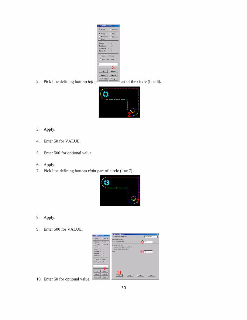
1. Main Menu> Solution> Define Loads> Apply> Structural> Pressure> On Lines
30
2. Pick line defining bottom left p art of the circle (line 6).
3. Apply.
4. Enter 50 for VALUE.
5. Enter 500 for optional value.
6. Apply. 7. Pick line defining bottom right part of circle (line 7).
8. Apply.
9. Enter 500 for VALUE.
10. Enter 50 for optional value.
31
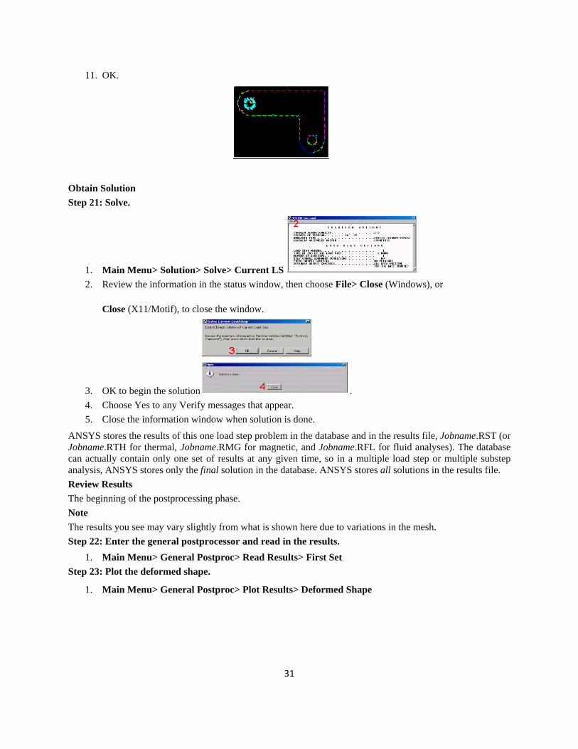
11. OK.
Obtain Solution Step 21: Solve.
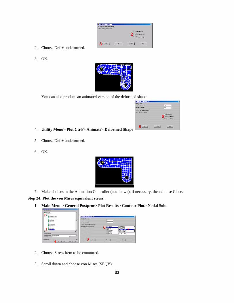
1. Main Menu> Solution> Solve> Current LS 2. Review the information in the status window, then choose File> Close (Windows), or
Close (X11/Motif), to close the window.
3. OK to begin the solution . 4. Choose Yes to any Verify messages that appear. 5. Close the information window when solution is done.
ANSYS stores the results of this one load step problem in the database and in the results file, Jobname.RST (or Jobname.RTH for thermal, Jobname.RMG for magnetic, and Jobname.RFL for fluid analyses). The database can actually contain only one set of results at any given time, so in a multiple load step or multiple substep analysis, ANSYS stores only the final solution in the database. ANSYS stores all solutions in the results file. Review Results The beginning of the postprocessing phase. Note The results you see may vary slightly from what is shown here due to variations in the mesh. Step 22: Enter the general postprocessor and read in the results.
1. Main Menu> General Postproc> Read Results> First Set Step 23: Plot the deformed shape.
1. Main Menu> General Postproc> Plot Results> Deformed Shape
32
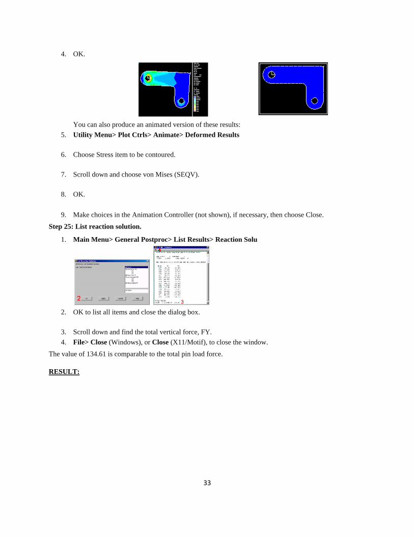
2. Choose Def + undeformed.
3. OK.
You can also produce an animated version of the deformed shape:
4. Utility Menu> Plot Ctrls> Animate> Deformed Shape
5. Choose Def + undeformed.
6. OK.
7. Make choices in the Animation Controller (not shown), if necessary, then choose Close.
Step 24: Plot the von Mises equivalent stress.
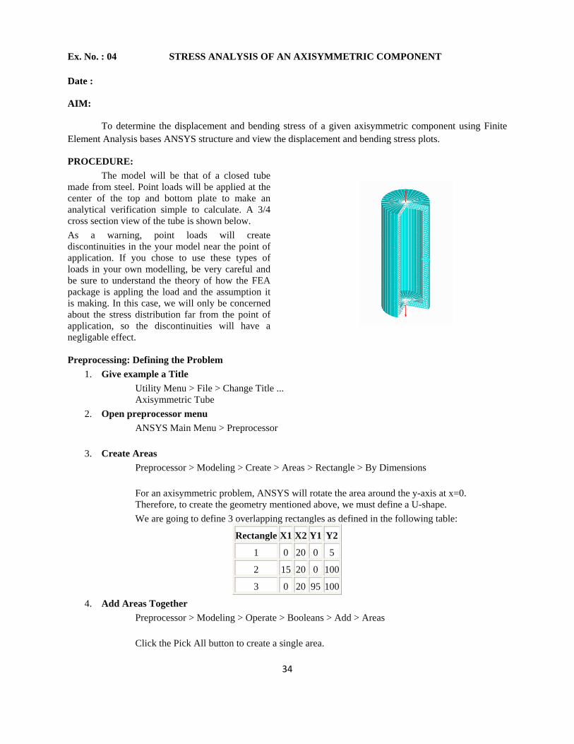
1. Main Menu> General Postproc> Plot Results> Contour Plot> Nodal Solu
2. Choose Stress item to be contoured.
3. Scroll down and choose von Mises (SEQV).
33
4. OK.
You can also produce an animated version of these results:
5. Utility Menu> Plot Ctrls> Animate> Deformed Results
6. Choose Stress item to be contoured.
7. Scroll down and choose von Mises (SEQV).
8. OK.
9. Make choices in the Animation Controller (not shown), if necessary, then choose Close.
Step 25: List reaction solution.
1. Main Menu> General Postproc> List Results> Reaction Solu
2. OK to list all items and close the dialog box.
3. Scroll down and find the total vertical force, FY. 4. File> Close (Windows), or Close (X11/Motif), to close the window.
The value of 134.61 is comparable to the total pin load force.
RESULT:
34
Ex. No. : 04 STRESS ANALYSIS OF AN AXISYMMETRIC COMPONENT
Date :
AIM:
To determine the displacement and bending stress of a given axisymmetric component using Finite Element Analysis bases ANSYS structure and view the displacement and bending stress plots.
PROCEDURE: The model will be that of a closed tube
made from steel. Point loads will be applied at the center of the top and bottom plate to make an analytical verification simple to calculate. A 3/4 cross section view of the tube is shown below. As a warning, point loads will create discontinuities in the your model near the point of application. If you chose to use these types of loads in your own modelling, be very careful and be sure to understand the theory of how the FEA package is appling the load and the assumption it is making. In this case, we will only be concerned about the stress distribution far from the point of application, so the discontinuities will have a negligable effect.
Preprocessing: Defining the Problem
1. Give example a Title Utility Menu > File > Change Title ... Axisymmetric Tube
2. Open preprocessor menu ANSYS Main Menu > Preprocessor
3. Create Areas Preprocessor > Modeling > Create > Areas > Rectangle > By Dimensions For an axisymmetric problem, ANSYS will rotate the area around the y-axis at x=0. Therefore, to create the geometry mentioned above, we must define a U-shape. We are going to define 3 overlapping rectangles as defined in the following table:
Rectangle X1 X2 Y1 Y2
1 0 20 0 5
2 15 20 0 100
3 0 20 95 100
4. Add Areas Together Preprocessor > Modeling > Operate > Booleans > Add > Areas Click the Pick All button to create a single area.
35
5. Define the Type of Element Preprocessor > Element Type > Add/Edit/Delete... For this problem we will use the PLANE2 (Structural, Solid, Triangle 6node) element. This element has 2 degrees of freedom (translation along the X and Y axes). Many elements support axisymmetry, however if the Ansys Elements Reference (which can be found in the help file) does not discuss axisymmetric applications for a particular element type, axisymmetry is not supported.
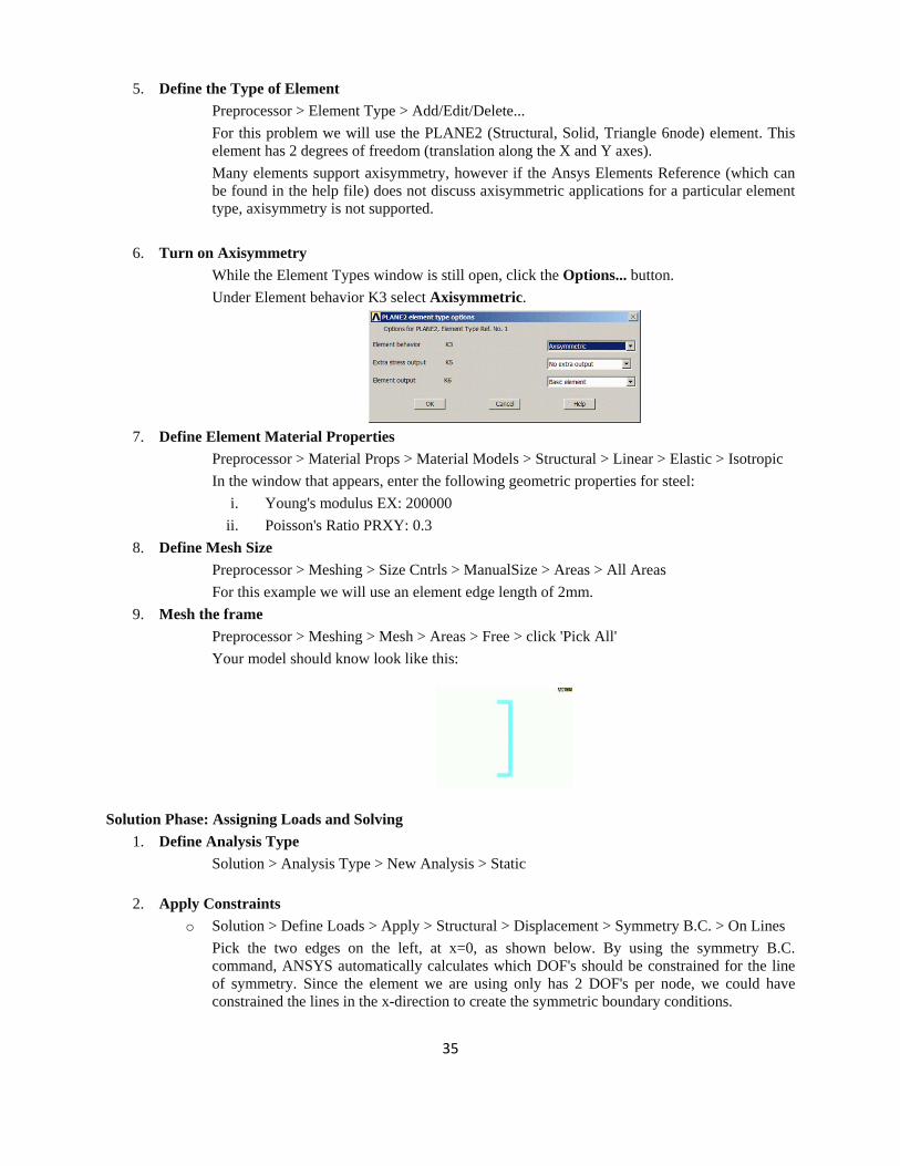
6. Turn on Axisymmetry
While the Element Types window is still open, click the Options... button. Under Element behavior K3 select Axisymmetric.
7. Define Element Material Properties
Preprocessor > Material Props > Material Models > Structural > Linear > Elastic > Isotropic In the window that appears, enter the following geometric properties for steel:
i. Young's modulus EX: 200000 ii. Poisson's Ratio PRXY: 0.3
8. Define Mesh Size Preprocessor > Meshing > Size Cntrls > ManualSize > Areas > All Areas For this example we will use an element edge length of 2mm.
9. Mesh the frame Preprocessor > Meshing > Mesh > Areas > Free > click 'Pick All' Your model should know look like this:
Solution Phase: Assigning Loads and Solving 1. Define Analysis Type
Solution > Analysis Type > New Analysis > Static
2. Apply Constraints o Solution > Define Loads > Apply > Structural > Displacement > Symmetry B.C. > On Lines
Pick the two edges on the left, at x=0, as shown below. By using the symmetry B.C. command, ANSYS automatically calculates which DOF's should be constrained for the line of symmetry. Since the element we are using only has 2 DOF's per node, we could have constrained the lines in the x-direction to create the symmetric boundary conditions.
36
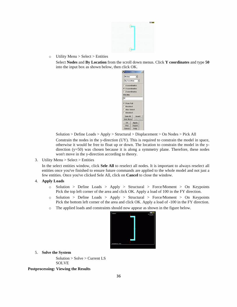
o Utility Menu > Select > Entities
Select Nodes and By Location from the scroll down menus. Click Y coordinates and type 50 into the input box as shown below, then click OK.
Solution > Define Loads > Apply > Structural > Displacement > On Nodes > Pick All Constrain the nodes in the y-direction (UY). This is required to constrain the model in space, otherwise it would be free to float up or down. The location to constrain the model in the y-direction (y=50) was chosen because it is along a symmetry plane. Therefore, these nodes won't move in the y-direction according to theory.
3. Utility Menu > Select > Entities In the select entities window, click Sele All to reselect all nodes. It is important to always reselect all entities once you've finished to ensure future commands are applied to the whole model and not just a few entities. Once you've clicked Sele All, click on Cancel to close the window.
4. Apply Loads o Solution > Define Loads > Apply > Structural > Force/Moment > On Keypoints
Pick the top left corner of the area and click OK. Apply a load of 100 in the FY direction. o Solution > Define Loads > Apply > Structural > Force/Moment > On Keypoints
Pick the bottom left corner of the area and click OK. Apply a load of -100 in the FY direction. o The applied loads and constraints should now appear as shown in the figure below.
5. Solve the System
Solution > Solve > Current LS SOLVE
Postprocessing: Viewing the Results
1. HHTh
2. D
3. P
RESULT
Hand CalculatiHand calculation
he stress acros
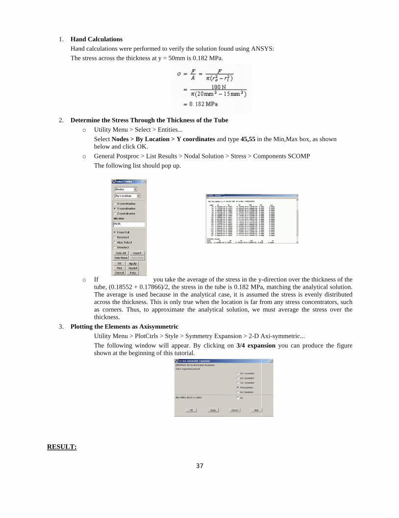
Determine the o Utility
Select Nbelow a
o GeneraThe fol
o If tube, (0The avacross as cornthickne
lotting the EleUtility The foshown
:
ions ns were perfor
ss the thickness
Stress ThrougMenu > SelectNodes > By Land click OK.
al Postproc > Lllowing list sho
0.18552 + 0.17verage is used the thickness. ners. Thus, to ess. ements as AxiMenu > PlotC
ollowing windoat the beginnin
rmed to verify ts at y = 50mm
gh the Thicknt > Entities... ocation > Y co
List Results > Nould pop up.
you take the 7866)/2, the strbecause in theThis is only trapproximate
symmetric Ctrls > Style > Sow will appeang of this tutor
37
the solution fouis 0.182 MPa.
ess of the Tub
oordinates and
Nodal Solution
average of theress in the tubee analytical carue when the lothe analytical
Symmetry Expar. By clickingrial.
und using ANS
be
d type 45,55 in
> Stress > Com
stress in the ye is 0.182 MPa
ase, it is assumocation is far f
solution, we
pansion > 2-D Ag on 3/4 expan
SYS:
n the Min,Max
mponents SCO
y-direction overa, matching the
med the stress ifrom any stressmust average
Axi-symmetricnsion you can
box, as shown
OMP
r the thickness e analytical solis evenly distrs concentrators the stress ov
c... n produce the
n
of the lution.
ributed s, such ver the
figure
38
Ex. No. : 05 STRESS ANALYSIS OF CANTILEVER BEAM
Date:
AIM:
To determine the displacement and bending stress of a given Cantilever Beam using Finite Element Analysis bases ANSYS structure and view the displacement and bending stress plots.
PROCEDURE:
The simplified version that will be used for this problem is that of a cantilever beam shown in the following figure:
Preprocessing: Defining the Problem
1. Give the Simplified Version a Title Utility Menu > File > Change Title (stress analysis of cantilever beam)
2. Enter Keypoints
For this simple example, these keypoints are the ends of the beam.
We are going to define 2 keypoints for the simplified structure as given in the following table
keypointcoordinate
x y z1 0 0 0 2 500 0 0
From the 'ANSYS Main Menu' select: Preprocessor > Modeling > Create > Keypoints > In Active CS
3. Form Lines
The two keypoints must now be connected to form a bar using a straight line. Select: Preprocessor > Modeling> Create > Lines > Lines > Straight Line. Pick keypoint #1 (i.e. click on it). It will now be marked by a small yellow box. Now pick keypoint #2. A permanent line will appear. When you're done, click on 'OK' in the 'Create Straight Line' window.
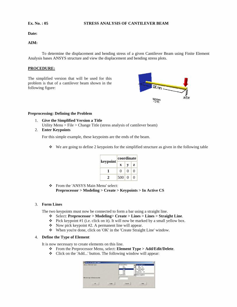
4. Define the Type of Element
It is now necessary to create elements on this line. From the Preprocessor Menu, select: Element Type > Add/Edit/Delete. Click on the 'Add...' button. The following window will appear:
39
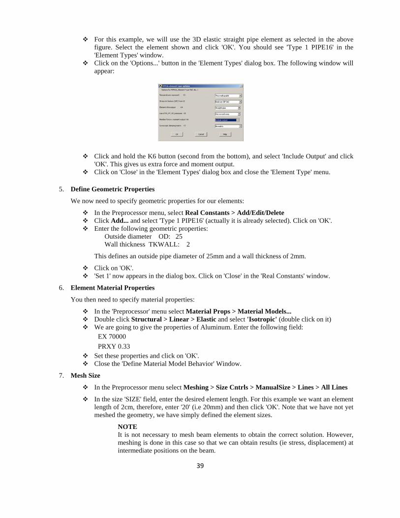
For this example, we will use the 3D elastic straight pipe element as selected in the above figure. Select the element shown and click 'OK'. You should see 'Type 1 PIPE16' in the 'Element Types' window.
Click on the 'Options...' button in the 'Element Types' dialog box. The following window will appear:
Click and hold the K6 button (second from the bottom), and select 'Include Output' and click 'OK'. This gives us extra force and moment output.
Click on 'Close' in the 'Element Types' dialog box and close the 'Element Type' menu.
5. Define Geometric Properties
We now need to specify geometric properties for our elements:
In the Preprocessor menu, select Real Constants > Add/Edit/Delete Click Add... and select 'Type 1 PIPE16' (actually it is already selected). Click on 'OK'. Enter the following geometric properties:
Outside diameter OD: 25 Wall thickness TKWALL: 2
This defines an outside pipe diameter of 25mm and a wall thickness of 2mm.
Click on 'OK'. 'Set 1' now appears in the dialog box. Click on 'Close' in the 'Real Constants' window.
6. Element Material Properties
You then need to specify material properties:
In the 'Preprocessor' menu select Material Props > Material Models... Double click Structural > Linear > Elastic and select 'Isotropic' (double click on it) We are going to give the properties of Aluminum. Enter the following field:
EX 70000 PRXY 0.33
Set these properties and click on 'OK'. Close the 'Define Material Model Behavior' Window.
7. Mesh Size
In the Preprocessor menu select Meshing > Size Cntrls > ManualSize > Lines > All Lines
In the size 'SIZE' field, enter the desired element length. For this example we want an element length of 2cm, therefore, enter '20' (i.e 20mm) and then click 'OK'. Note that we have not yet meshed the geometry, we have simply defined the element sizes.
NOTE It is not necessary to mesh beam elements to obtain the correct solution. However, meshing is done in this case so that we can obtain results (ie stress, displacement) at intermediate positions on the beam.
40
8. Mesh
Now the frame can be meshed.
In the 'Preprocessor' menu select Meshing > Mesh > Lines and click 'Pick All' in the 'Mesh Lines' Window
9. Saving Your Work
Utility Menu > File > Save as.... Select the name and location where you want to save your file.
Solution Phase: Assigning Loads and Solving
1. Define Analysis Type
From the Solution Menu, select 'Analysis Type > New Analysis'. Ensure that 'Static' is selected and click 'OK'.
2. Apply Constraints
In the Solution menu, select Define Loads > Apply > Structural > Displacement > On Keypoints
Select the left end of the rod (Keypoint 1) by clicking on it in the Graphics Window and click on 'OK' in the 'Apply U,ROT on KPs' window.
This location is fixed which means that all translational and rotational degrees of freedom (DOFs) are constrained. Therefore, select 'All DOF' by clicking on it and enter '0' in the Value field and click 'OK'.
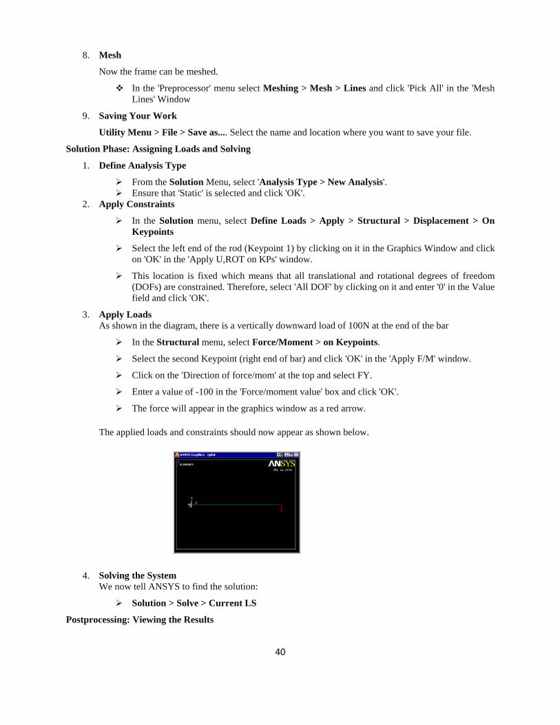
3. Apply Loads As shown in the diagram, there is a vertically downward load of 100N at the end of the bar
In the Structural menu, select Force/Moment > on Keypoints.
Select the second Keypoint (right end of bar) and click 'OK' in the 'Apply F/M' window.
Click on the 'Direction of force/mom' at the top and select FY.
Enter a value of -100 in the 'Force/moment value' box and click 'OK'.
The force will appear in the graphics window as a red arrow.
The applied loads and constraints should now appear as shown below.
4. Solving the System We now tell ANSYS to find the solution:
Solution > Solve > Current LS
Postprocessing: Viewing the Results
41
1. Hand Calculations
Now, since the purpose of this exercise was to verify the results - we need to calculate what we should find.
Deflection:
The maximum deflection occurs at the end of the rod and was found to be 6.2mm as shown above.
Stress:
The maximum stress occurs at the base of the rod and was found to be 64.9MPa as shown above (pure bending stress).
2. Results Using ANSYS
Deformation
from the Main Menu select General Postproc from the 'ANSYS Main Menu'. In this menu you will find a variety of options, the two which we will deal with now are 'Plot Results' and 'List Results'
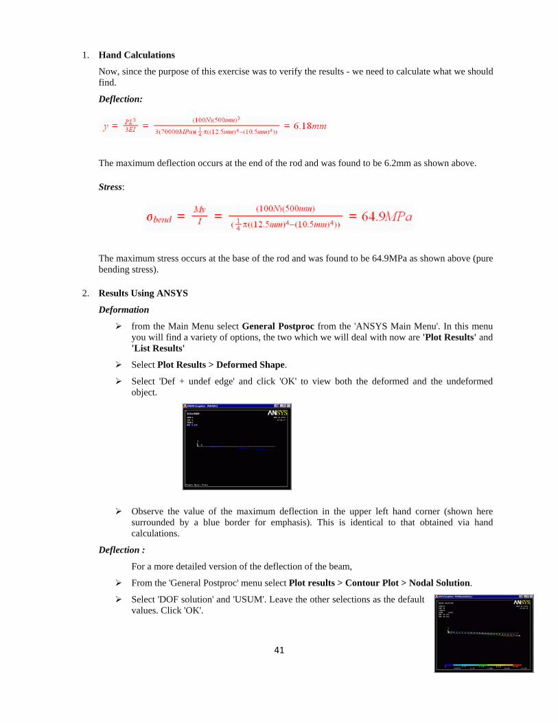
Select Plot Results > Deformed Shape.
Select 'Def + undef edge' and click 'OK' to view both the deformed and the undeformed object.
Observe the value of the maximum deflection in the upper left hand corner (shown here surrounded by a blue border for emphasis). This is identical to that obtained via hand calculations.
Deflection :
For a more detailed version of the deflection of the beam,
From the 'General Postproc' menu select Plot results > Contour Plot > Nodal Solution.
Select 'DOF solution' and 'USUM'. Leave the other selections as the default values. Click 'OK'.

42
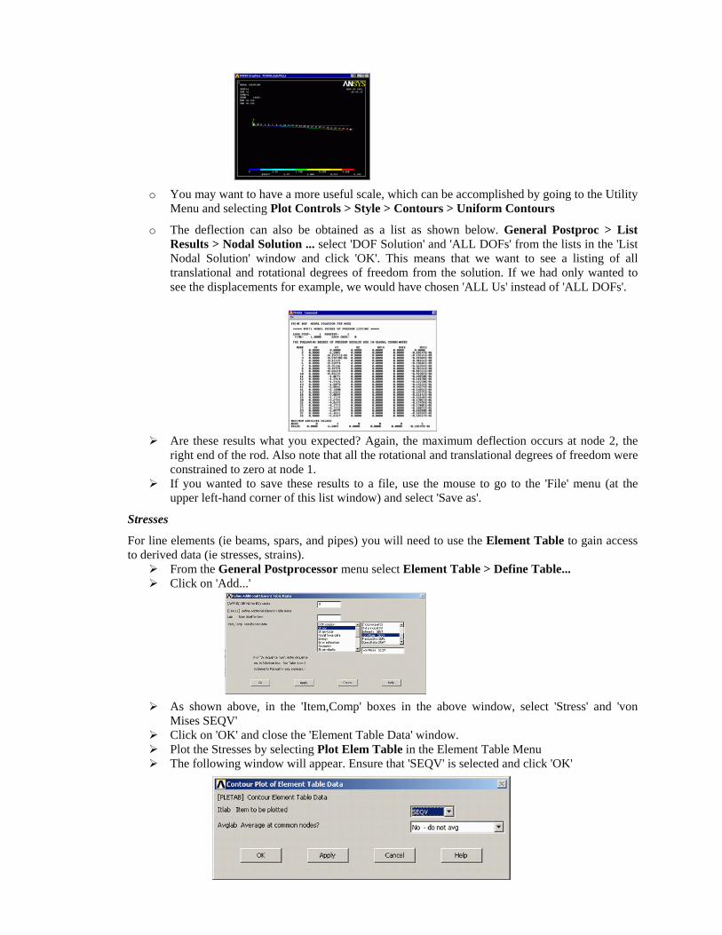
o You may want to have a more useful scale, which can be accomplished by going to the Utility Menu and selecting Plot Controls > Style > Contours > Uniform Contours
o The deflection can also be obtained as a list as shown below. General Postproc > List Results > Nodal Solution ... select 'DOF Solution' and 'ALL DOFs' from the lists in the 'List Nodal Solution' window and click 'OK'. This means that we want to see a listing of all translational and rotational degrees of freedom from the solution. If we had only wanted to see the displacements for example, we would have chosen 'ALL Us' instead of 'ALL DOFs'.
Are these results what you expected? Again, the maximum deflection occurs at node 2, the right end of the rod. Also note that all the rotational and translational degrees of freedom were constrained to zero at node 1.
If you wanted to save these results to a file, use the mouse to go to the 'File' menu (at the upper left-hand corner of this list window) and select 'Save as'.
Stresses
For line elements (ie beams, spars, and pipes) you will need to use the Element Table to gain access to derived data (ie stresses, strains).
From the General Postprocessor menu select Element Table > Define Table... Click on 'Add...'
As shown above, in the 'Item,Comp' boxes in the above window, select 'Stress' and 'von Mises SEQV'
Click on 'OK' and close the 'Element Table Data' window. Plot the Stresses by selecting Plot Elem Table in the Element Table Menu The following window will appear. Ensure that 'SEQV' is selected and click 'OK'
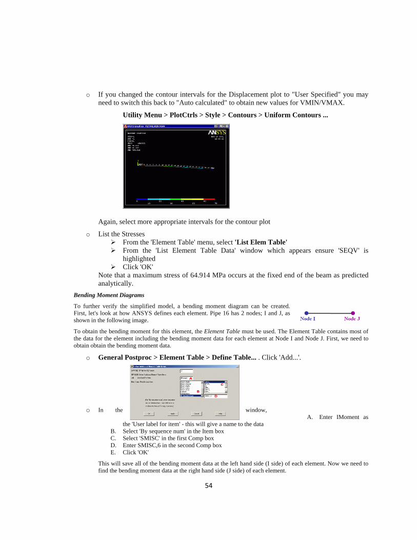
o If you changed the contour intervals for the Displacement plot to "User Specified" you may need to switch this back to "Auto calculated" to obtain new values for VMIN/VMAX.
43
Utility Menu > PlotCtrls > Style > Contours > Uniform Contours...
Again, select more appropriate intervals for the contour plot
o List the Stresses From the 'Element Table' menu, select 'List Elem Table' From the 'List Element Table Data' window which appears ensure 'SEQV' is
highlighted Click 'OK'
Note that a maximum stress of 64.914 MPa occurs at the fixed end of the beam as predicted analytically.
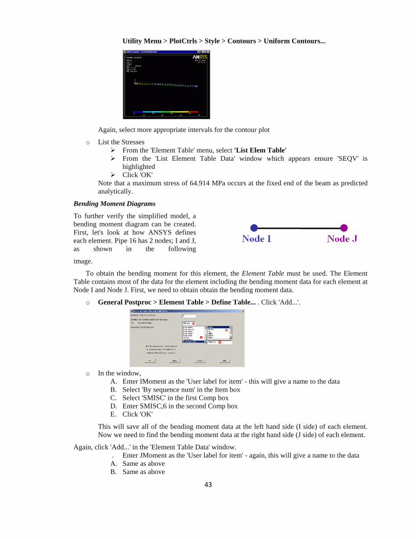
Bending Moment Diagrams
To further verify the simplified model, a bending moment diagram can be created. First, let's look at how ANSYS defines each element. Pipe 16 has 2 nodes; I and J, as shown in the following
image.
To obtain the bending moment for this element, the Element Table must be used. The Element Table contains most of the data for the element including the bending moment data for each element at Node I and Node J. First, we need to obtain obtain the bending moment data.
o General Postproc > Element Table > Define Table... . Click 'Add...'.
o In the window, A. Enter IMoment as the 'User label for item' - this will give a name to the data B. Select 'By sequence num' in the Item box C. Select 'SMISC' in the first Comp box D. Enter SMISC,6 in the second Comp box E. Click 'OK'
This will save all of the bending moment data at the left hand side (I side) of each element. Now we need to find the bending moment data at the right hand side (J side) of each element.
Again, click 'Add...' in the 'Element Table Data' window. . Enter JMoment as the 'User label for item' - again, this will give a name to the data A. Same as above B. Same as above
44
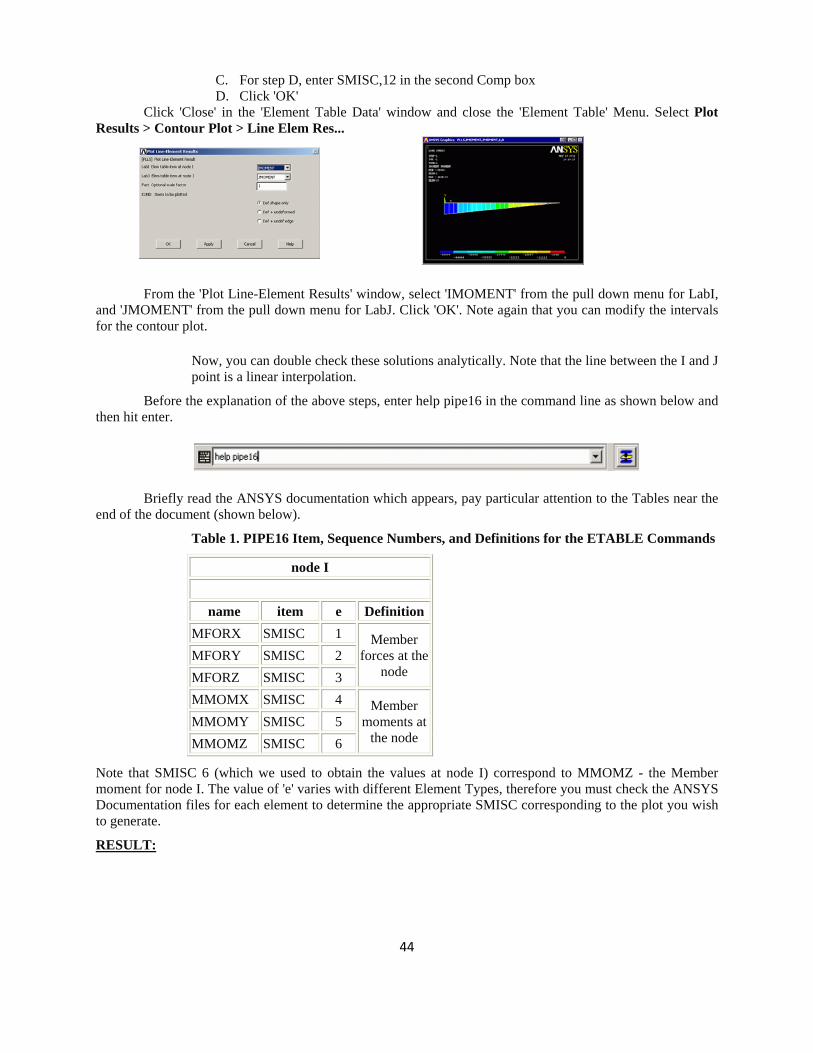
C. For step D, enter SMISC,12 in the second Comp box D. Click 'OK'
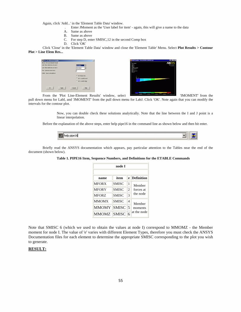
Click 'Close' in the 'Element Table Data' window and close the 'Element Table' Menu. Select Plot Results > Contour Plot > Line Elem Res...
From the 'Plot Line-Element Results' window, select 'IMOMENT' from the pull down menu for LabI, and 'JMOMENT' from the pull down menu for LabJ. Click 'OK'. Note again that you can modify the intervals for the contour plot.
Now, you can double check these solutions analytically. Note that the line between the I and J point is a linear interpolation.
Before the explanation of the above steps, enter help pipe16 in the command line as shown below and then hit enter.
Briefly read the ANSYS documentation which appears, pay particular attention to the Tables near the end of the document (shown below).
Table 1. PIPE16 Item, Sequence Numbers, and Definitions for the ETABLE Commands
node I
name item e DefinitionMFORX SMISC 1 Member
forces at the node
MFORY SMISC 2 MFORZ SMISC 3 MMOMX SMISC 4 Member
moments at the node
MMOMY SMISC 5 MMOMZ SMISC 6
Note that SMISC 6 (which we used to obtain the values at node I) correspond to MMOMZ - the Member moment for node I. The value of 'e' varies with different Element Types, therefore you must check the ANSYS Documentation files for each element to determine the appropriate SMISC corresponding to the plot you wish to generate.
RESULT:
45
Ex. No. : 06 STRESS ANALYSIS OF SIMPLY SUPPORTED BEAM
Date:
AIM:
To determine the displacement and bending stress of a given simply supported beam using Finite Element Analysis bases ANSYS structure and view the displacement and bending stress plots.
PROCEDURE:
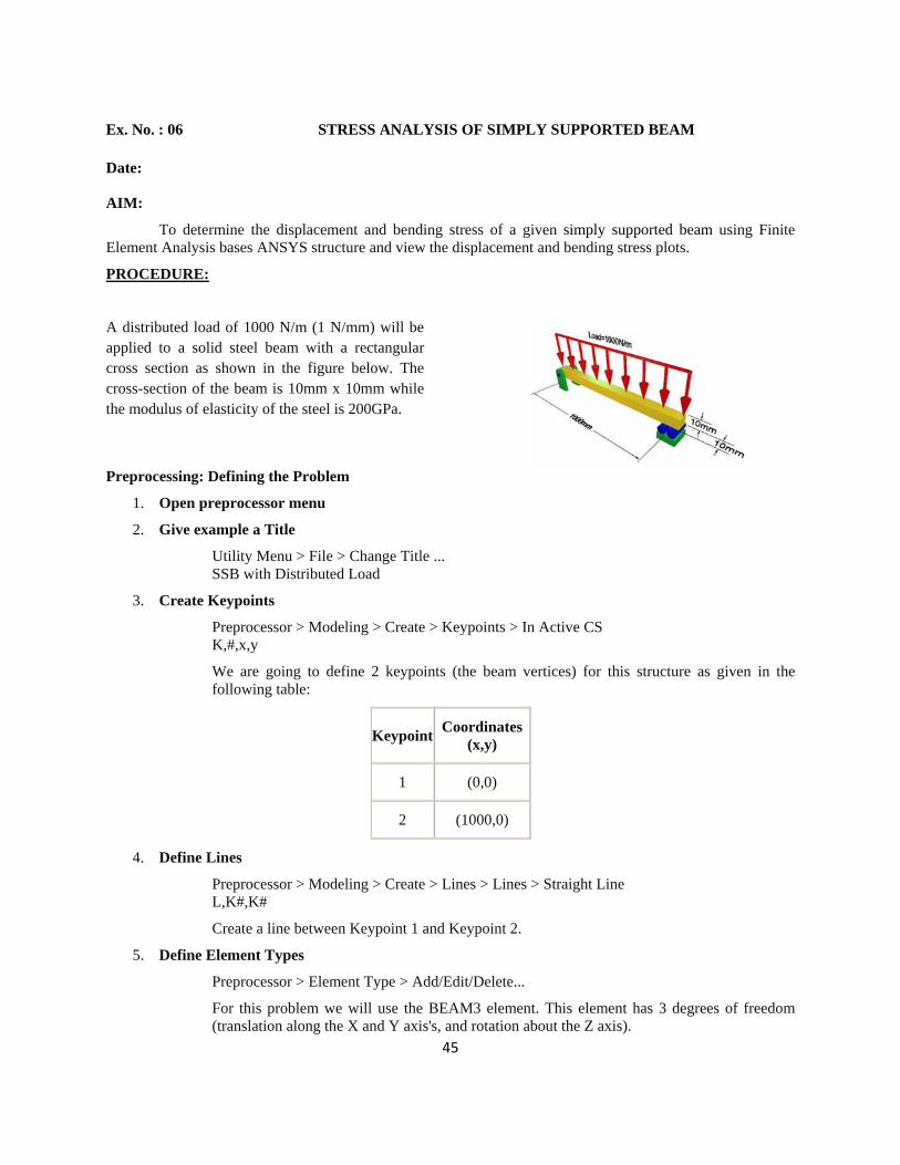
A distributed load of 1000 N/m (1 N/mm) will be applied to a solid steel beam with a rectangular cross section as shown in the figure below. The cross-section of the beam is 10mm x 10mm while the modulus of elasticity of the steel is 200GPa.
Preprocessing: Defining the Problem
1. Open preprocessor menu
2. Give example a Title
Utility Menu > File > Change Title ... SSB with Distributed Load
3. Create Keypoints
Preprocessor > Modeling > Create > Keypoints > In Active CS K,#,x,y
We are going to define 2 keypoints (the beam vertices) for this structure as given in the following table:
Keypoint Coordinates (x,y)
1 (0,0)
2 (1000,0)
4. Define Lines
Preprocessor > Modeling > Create > Lines > Lines > Straight Line L,K#,K#
Create a line between Keypoint 1 and Keypoint 2.
5. Define Element Types
Preprocessor > Element Type > Add/Edit/Delete...
For this problem we will use the BEAM3 element. This element has 3 degrees of freedom (translation along the X and Y axis's, and rotation about the Z axis).

46
6. Define Real Constants
Preprocessor > Real Constants... > Add...
In the 'Real Constants for BEAM3' window, enter the following geometric properties:
i. Cross-sectional area AREA: 100
ii. Area Moment of Inertia IZZ: 833.333
iii. Total beam height HEIGHT: 10
This defines an element with a solid rectangular cross section 10mm x 10mm.
7. Define Element Material Properties
Preprocessor > Material Props > Material Models > Structural > Linear > Elastic > Isotropic
In the window that appears, enter the following geometric properties for steel:
i. Young's modulus EX: 200000
ii. Poisson's Ratio PRXY: 0.3
8. Define Mesh Size
Preprocessor > Meshing > Size Cntrls > ManualSize > Lines > All Lines... For this example we will use an element length of 100mm.
9. Mesh the frame
Preprocessor > Meshing > Mesh > Lines > click 'Pick All'
10. Plot Elements
Utility Menu > Plot > Elements
You may also wish to turn on element numbering and turn off keypoint numbering
Utility Menu > PlotCtrls > Numbering...
Solution Phase: Assigning Loads and Solving
1. Define Analysis Type
Solution > Analysis Type > New Analysis > Static
2. Apply Constraints
Solution > Define Loads > Apply > Structural > Displacement > On Keypoints
Pin Keypoint 1 (ie UX and UY constrained) and fix Keypoint 2 in the y direction (UY constrained).
3. Apply Loads
We will apply a distributed load, of 1000 N/m or 1 N/mm, over the entire length of the beam.
47
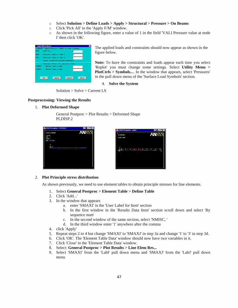
o Select Solution > Define Loads > Apply > Structural > Pressure > On Beams o Click 'Pick All' in the 'Apply F/M' window. o As shown in the following figure, enter a value of 1 in the field 'VALI Pressure value at node
I' then click 'OK'.
The applied loads and constraints should now appear as shown in the figure below.
Note: To have the constraints and loads appear each time you select 'Replot' you must change some settings. Select Utility Menu > PlotCtrls > Symbols.... In the window that appears, select 'Pressures' in the pull down menu of the 'Surface Load Symbols' section.
4. Solve the System
Solution > Solve > Current LS
Postprocessing: Viewing the Results
1. Plot Deformed Shape
General Postproc > Plot Results > Deformed Shape PLDISP.2
2. Plot Principle stress distribution
As shown previously, we need to use element tables to obtain principle stresses for line elements.
1. Select General Postproc > Element Table > Define Table 2. Click 'Add...' 3. In the window that appears
a. enter 'SMAXI' in the 'User Label for Item' section b. In the first window in the 'Results Data Item' section scroll down and select 'By
sequence num' c. In the second window of the same section, select 'NMISC, ' d. In the third window enter '1' anywhere after the comma
4. click 'Apply' 5. Repeat steps 2 to 4 but change 'SMAXI' to 'SMAXJ' in step 3a and change '1' to '3' in step 3d. 6. Click 'OK'. The 'Element Table Data' window should now have two variables in it. 7. Click 'Close' in the 'Element Table Data' window. 8. Select: General Postproc > Plot Results > Line Elem Res... 9. Select 'SMAXI' from the 'LabI' pull down menu and 'SMAXJ' from the 'LabJ' pull down
menu
48
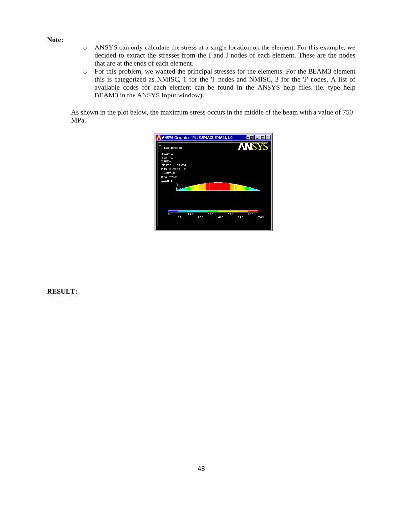
Note: o ANSYS can only calculate the stress at a single location on the element. For this example, we
decided to extract the stresses from the I and J nodes of each element. These are the nodes that are at the ends of each element.
o For this problem, we wanted the principal stresses for the elements. For the BEAM3 element this is categorized as NMISC, 1 for the 'I' nodes and NMISC, 3 for the 'J' nodes. A list of available codes for each element can be found in the ANSYS help files. (ie. type help BEAM3 in the ANSYS Input window).
As shown in the plot below, the maximum stress occurs in the middle of the beam with a value of 750 MPa.
RESULT:
49
Ex. No. : 07 STRESS ANALYSIS OF FIXED BEAM
Date:
AIM:
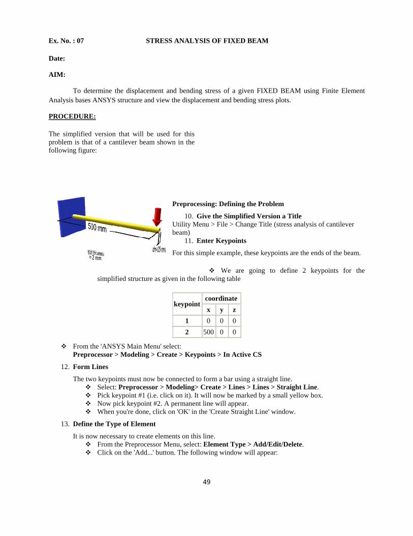
To determine the displacement and bending stress of a given FIXED BEAM using Finite Element Analysis bases ANSYS structure and view the displacement and bending stress plots.
PROCEDURE:
The simplified version that will be used for this problem is that of a cantilever beam shown in the following figure:
Preprocessing: Defining the Problem
10. Give the Simplified Version a Title Utility Menu > File > Change Title (stress analysis of cantilever beam)
11. Enter Keypoints
For this simple example, these keypoints are the ends of the beam.
We are going to define 2 keypoints for the simplified structure as given in the following table
keypointcoordinatex y z
1 0 0 0 2 500 0 0
From the 'ANSYS Main Menu' select: Preprocessor > Modeling > Create > Keypoints > In Active CS
12. Form Lines
The two keypoints must now be connected to form a bar using a straight line. Select: Preprocessor > Modeling> Create > Lines > Lines > Straight Line. Pick keypoint #1 (i.e. click on it). It will now be marked by a small yellow box. Now pick keypoint #2. A permanent line will appear. When you're done, click on 'OK' in the 'Create Straight Line' window.
13. Define the Type of Element
It is now necessary to create elements on this line. From the Preprocessor Menu, select: Element Type > Add/Edit/Delete. Click on the 'Add...' button. The following window will appear:
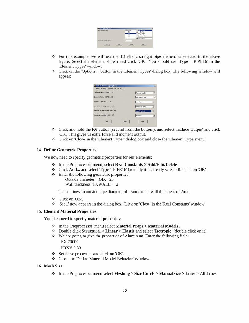
50
For this example, we will use the 3D elastic straight pipe element as selected in the above figure. Select the element shown and click 'OK'. You should see 'Type 1 PIPE16' in the 'Element Types' window.
Click on the 'Options...' button in the 'Element Types' dialog box. The following window will appear:
Click and hold the K6 button (second from the bottom), and select 'Include Output' and click 'OK'. This gives us extra force and moment output.
Click on 'Close' in the 'Element Types' dialog box and close the 'Element Type' menu.
14. Define Geometric Properties
We now need to specify geometric properties for our elements:
In the Preprocessor menu, select Real Constants > Add/Edit/Delete Click Add... and select 'Type 1 PIPE16' (actually it is already selected). Click on 'OK'. Enter the following geometric properties:
Outside diameter OD: 25 Wall thickness TKWALL: 2
This defines an outside pipe diameter of 25mm and a wall thickness of 2mm.
Click on 'OK'. 'Set 1' now appears in the dialog box. Click on 'Close' in the 'Real Constants' window.
15. Element Material Properties
You then need to specify material properties:
In the 'Preprocessor' menu select Material Props > Material Models... Double click Structural > Linear > Elastic and select 'Isotropic' (double click on it) We are going to give the properties of Aluminum. Enter the following field:
EX 70000 PRXY 0.33
Set these properties and click on 'OK'. Close the 'Define Material Model Behavior' Window.
16. Mesh Size
In the Preprocessor menu select Meshing > Size Cntrls > ManualSize > Lines > All Lines
51
In the size 'SIZE' field, enter the desired element length. For this example we want an element length of 2cm, therefore, enter '20' (i.e 20mm) and then click 'OK'. Note that we have not yet meshed the geometry, we have simply defined the element sizes.
NOTE It is not necessary to mesh beam elements to obtain the correct solution. However, meshing is done in this case so that we can obtain results (ie stress, displacement) at intermediate positions on the beam.
17. Mesh
Now the frame can be meshed.
In the 'Preprocessor' menu select Meshing > Mesh > Lines and click 'Pick All' in the 'Mesh Lines' Window
18. Saving Your Work
Utility Menu > File > Save as.... Select the name and location where you want to save your file.
Solution Phase: Assigning Loads and Solving
5. Define Analysis Type
From the Solution Menu, select 'Analysis Type > New Analysis'. Ensure that 'Static' is selected and click 'OK'.
6. Apply Constraints
In the Solution menu, select Define Loads > Apply > Structural > Displacement > On Keypoints
Select the left end of the rod (Keypoint 1) and Select the right end of the rod (Keypoint 2) by clicking on it in the Graphics Window and click on 'OK' in the 'Apply U,ROT on KPs' window.
This location is fixed which means that all translational and rotational degrees of freedom (DOFs) are constrained. Therefore, select 'All DOF' by clicking on it and enter '0' in the Value field and click 'OK'.
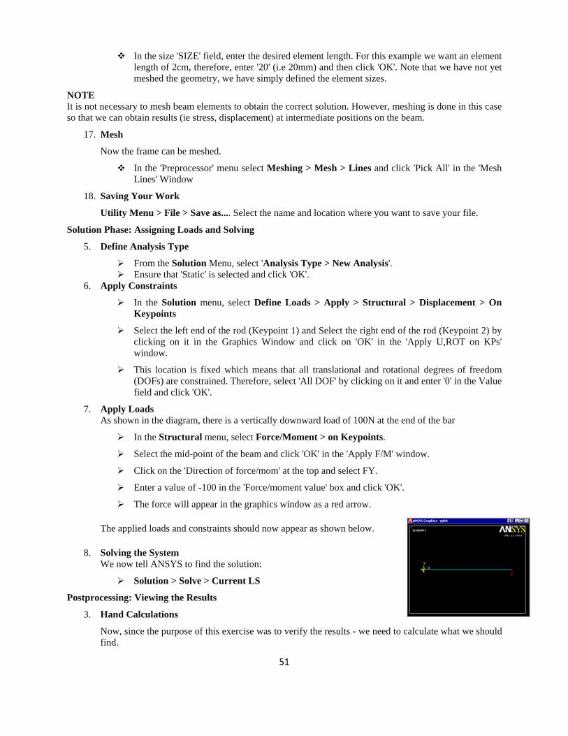
7. Apply Loads As shown in the diagram, there is a vertically downward load of 100N at the end of the bar
In the Structural menu, select Force/Moment > on Keypoints.
Select the mid-point of the beam and click 'OK' in the 'Apply F/M' window.
Click on the 'Direction of force/mom' at the top and select FY.
Enter a value of -100 in the 'Force/moment value' box and click 'OK'.
The force will appear in the graphics window as a red arrow.
The applied loads and constraints should now appear as shown below.
8. Solving the System We now tell ANSYS to find the solution:
Solution > Solve > Current LS
Postprocessing: Viewing the Results
3. Hand Calculations
Now, since the purpose of this exercise was to verify the results - we need to calculate what we should find.
52
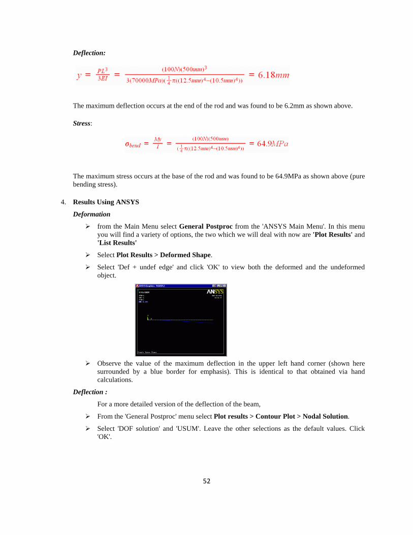
Deflection:
The maximum deflection occurs at the end of the rod and was found to be 6.2mm as shown above.
Stress:
The maximum stress occurs at the base of the rod and was found to be 64.9MPa as shown above (pure bending stress).
4. Results Using ANSYS
Deformation
from the Main Menu select General Postproc from the 'ANSYS Main Menu'. In this menu you will find a variety of options, the two which we will deal with now are 'Plot Results' and 'List Results'
Select Plot Results > Deformed Shape.
Select 'Def + undef edge' and click 'OK' to view both the deformed and the undeformed object.
Observe the value of the maximum deflection in the upper left hand corner (shown here surrounded by a blue border for emphasis). This is identical to that obtained via hand calculations.
Deflection :
For a more detailed version of the deflection of the beam,
From the 'General Postproc' menu select Plot results > Contour Plot > Nodal Solution.
Select 'DOF solution' and 'USUM'. Leave the other selections as the default values. Click 'OK'.
53
o You may want to have a more useful scale, which can be accomplished by going to the Utility Menu and selecting Plot Controls > Style > Contours > Uniform Contours
o The deflection can also be obtained as a list as shown below. General Postproc > List Results > Nodal Solution ... select 'DOF Solution' and 'ALL DOFs' from the lists in the 'List Nodal Solution' window and click 'OK'. This means that we want to see a listing of all translational and rotational degrees of freedom from the solution. If we had only wanted to see the displacements for example, we would have chosen 'ALL Us' instead of 'ALL DOFs'.
Are these results what you expected? Again, the maximum deflection occurs at node 2, the right end of the rod. Also note that all the rotational and translational degrees of freedom were constrained to zero at node 1.
If you wanted to save these results to a file, use the mouse to go to the 'File' menu (at the upper left-hand corner of this list window) and select 'Save as'.
Stresses
For line elements (ie beams, spars, and pipes) you will need to use the Element Table to gain access to derived data (ie stresses, strains).
From the General Postprocessor menu select Element Table > Define Table... Click on 'Add...'
As shown above, in the 'Item,Comp' boxes in the above window, select 'Stress' and 'von Mises SEQV'
Click on 'OK' and close the 'Element Table Data' window. Plot the Stresses by selecting Plot Elem Table in the Element Table Menu The following window will appear. Ensure that 'SEQV' is selected and click 'OK'
54
o If you changed the contour intervals for the Displacement plot to "User Specified" you may need to switch this back to "Auto calculated" to obtain new values for VMIN/VMAX.
Utility Menu > PlotCtrls > Style > Contours > Uniform Contours ...
Again, select more appropriate intervals for the contour plot
o List the Stresses From the 'Element Table' menu, select 'List Elem Table' From the 'List Element Table Data' window which appears ensure 'SEQV' is
highlighted Click 'OK'
Note that a maximum stress of 64.914 MPa occurs at the fixed end of the beam as predicted analytically.
Bending Moment Diagrams
To further verify the simplified model, a bending moment diagram can be created. First, let's look at how ANSYS defines each element. Pipe 16 has 2 nodes; I and J, as shown in the following image.
To obtain the bending moment for this element, the Element Table must be used. The Element Table contains most of the data for the element including the bending moment data for each element at Node I and Node J. First, we need to obtain obtain the bending moment data.
o General Postproc > Element Table > Define Table... . Click 'Add...'.
o In the window, A. Enter IMoment as
the 'User label for item' - this will give a name to the data B. Select 'By sequence num' in the Item box C. Select 'SMISC' in the first Comp box D. Enter SMISC,6 in the second Comp box E. Click 'OK'
This will save all of the bending moment data at the left hand side (I side) of each element. Now we need to find the bending moment data at the right hand side (J side) of each element.
55
Again, click 'Add...' in the 'Element Table Data' window. . Enter JMoment as the 'User label for item' - again, this will give a name to the data A. Same as above B. Same as above C. For step D, enter SMISC,12 in the second Comp box D. Click 'OK'
Click 'Close' in the 'Element Table Data' window and close the 'Element Table' Menu. Select Plot Results > Contour Plot > Line Elem Res...
From the 'Plot Line-Element Results' window, select 'IMOMENT' from the pull down menu for LabI, and 'JMOMENT' from the pull down menu for LabJ. Click 'OK'. Note again that you can modify the intervals for the contour plot.
Now, you can double check these solutions analytically. Note that the line between the I and J point is a linear interpolation.
Before the explanation of the above steps, enter help pipe16 in the command line as shown below and then hit enter.
Briefly read the ANSYS documentation which appears, pay particular attention to the Tables near the end of the document (shown below).
Table 1. PIPE16 Item, Sequence Numbers, and Definitions for the ETABLE Commands
node I
name item e DefinitionMFORX SMISC 1 Member
forces at the node
MFORY SMISC 2
MFORZ SMISC 3
MMOMX SMISC 4Member moments
at the nodeMMOMY SMISC 5MMOMZ SMISC 6
Note that SMISC 6 (which we used to obtain the values at node I) correspond to MMOMZ - the Member moment for node I. The value of 'e' varies with different Element Types, therefore you must check the ANSYS Documentation files for each element to determine the appropriate SMISC corresponding to the plot you wish to generate.
RESULT:
56
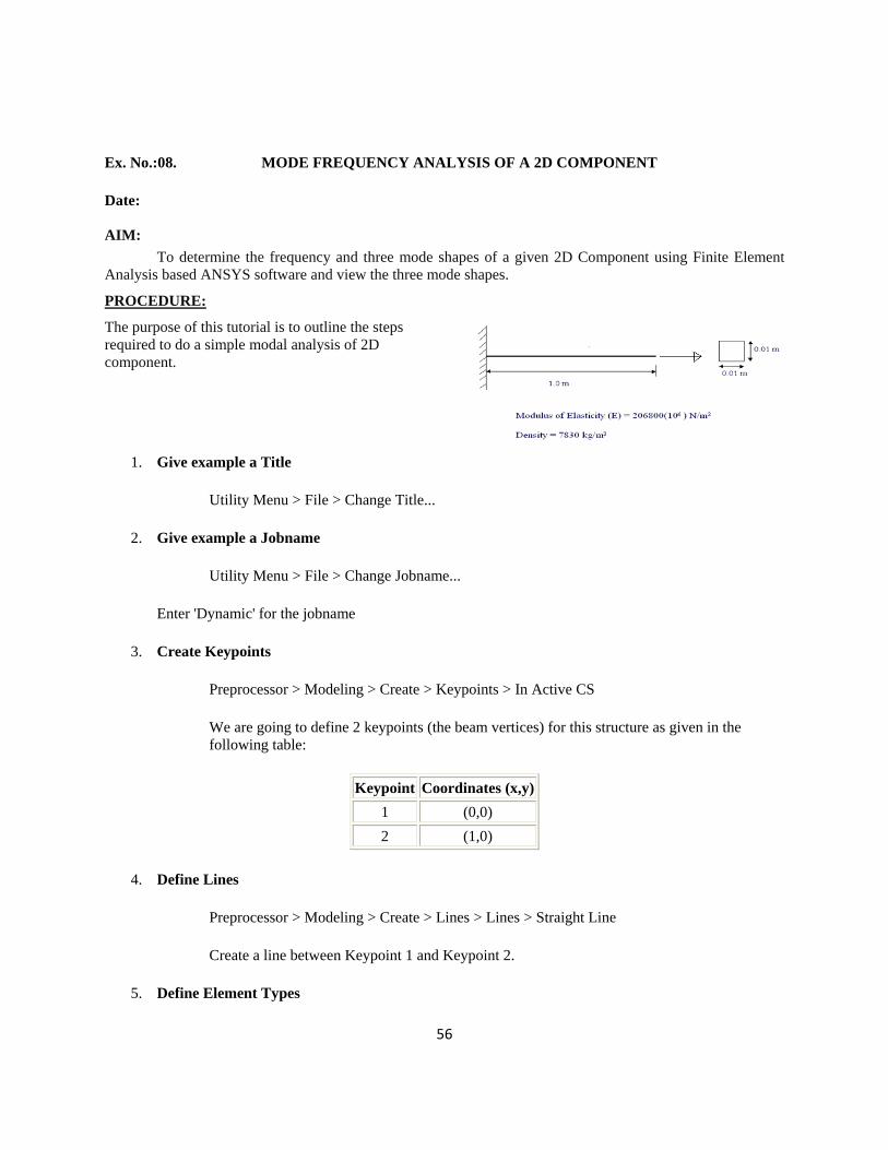
Ex. No.:08. MODE FREQUENCY ANALYSIS OF A 2D COMPONENT
Date:
AIM: To determine the frequency and three mode shapes of a given 2D Component using Finite Element Analysis based ANSYS software and view the three mode shapes.
PROCEDURE:
The purpose of this tutorial is to outline the steps required to do a simple modal analysis of 2D component.
1. Give example a Title
Utility Menu > File > Change Title...
2. Give example a Jobname
Utility Menu > File > Change Jobname...
Enter 'Dynamic' for the jobname
3. Create Keypoints
Preprocessor > Modeling > Create > Keypoints > In Active CS
We are going to define 2 keypoints (the beam vertices) for this structure as given in the following table:
Keypoint Coordinates (x,y)1 (0,0) 2 (1,0)
4. Define Lines
Preprocessor > Modeling > Create > Lines > Lines > Straight Line
Create a line between Keypoint 1 and Keypoint 2.
5. Define Element Types

57
Preprocessor > Element Type > Add/Edit/Delete...
For this problem we will use the BEAM3 (Beam 2D elastic) element. This element has 3 degrees of freedom (translation along the X and Y axis's, and rotation about the Z axis). With only 3 degrees of freedom, the BEAM3 element can only be used in 2D analysis.
6. Define Real Constants
Preprocessor > Real Constants... > Add...
In the 'Real Constants for BEAM3' window, enter the following geometric properties:
i. Cross-sectional area AREA: 0.0001 ii. Area Moment of Inertia IZZ: 8.33e-10
iii. Total beam height HEIGHT: 0.01
This defines an element with a solid rectangular cross section 0.01 m x 0.01 m.
7. Define Element Material Properties
Preprocessor > Material Props > Material Models > Structural > Linear > Elastic > Isotropic
In the window that appears, enter the following geometric properties for steel:
i. Young's modulus EX: 2.068e11 ii. Poisson's Ratio PRXY: 0.3
To enter the density of the material, double click on 'Linear' followed by 'Density' in the 'Define Material Model Behavior' Window
Enter a density of 7830
Note: For dynamic analysis, both the stiffness and the material density have to be specified.
8. Define Mesh Size
Preprocessor > Meshing > Size Cntrls > ManualSize > Lines > All Lines...
For this example we will specify 10 element divisions along the line.
9. Mesh the frame
Preprocessor > Meshing > Mesh > Lines > click 'Pick All'
Solution: Assigning Loads and Solving
1. Define Analysis Type
Solution > Analysis Type > New Analysis > Modal
2. Set options for analysis type:

58
o Select: Solution > Analysis Type > Analysis Options.. The following window will appear
o As shown, select the Subspace method and enter 5 in the 'No. of modes to extract' o Check the box beside 'Expand mode shapes' and enter 5 in the 'No. of modes to expand' o Click 'OK'
Note that the default mode extraction method chosen is the Reduced Method. This is the fastest method as it reduces the system matrices to only consider the Master Degrees of Freedom (see below). The Subspace Method extracts modes for all DOF's. It is therefore more exact but, it also takes longer to compute (especially when the complex geometries).
o The following window will then appear
For a better understanding of these options see the Commands manual.
o For this problem, we will use the default options so click on OK.
3. Apply Constraints
Solution > Define Loads > Apply > Structural > Displacement > On Keypoints
Fix Keypoint 1 (ie all DOFs constrained).
Solution > Define Loads > Apply > Structural > Displacement > On Keypoints
Fix Keypoint 2 (only Uy is constrained).
59
4. Solve the System
Solution > Solve > Current LS
Postprocessing: Viewing the Results
1. Verify extracted modes against theoretical predictions
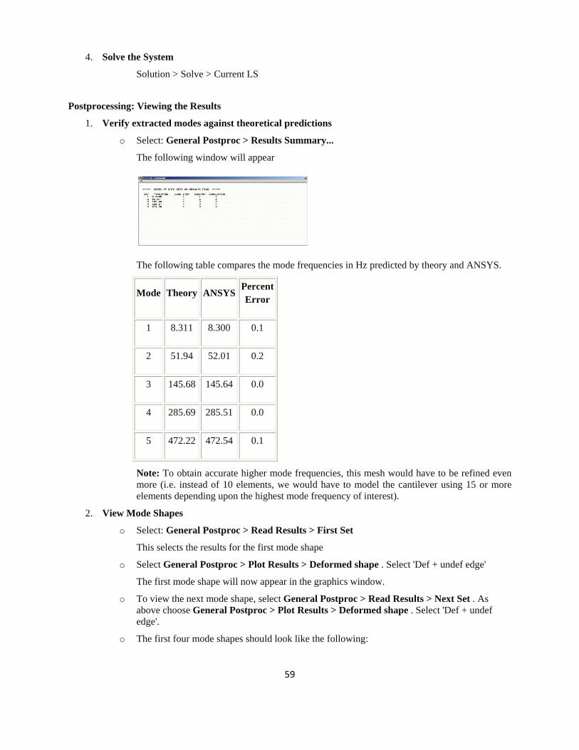
o Select: General Postproc > Results Summary...
The following window will appear
The following table compares the mode frequencies in Hz predicted by theory and ANSYS.
Mode Theory ANSYSPercent Error
1 8.311 8.300 0.1
2 51.94 52.01 0.2
3 145.68 145.64 0.0
4 285.69 285.51 0.0
5 472.22 472.54 0.1
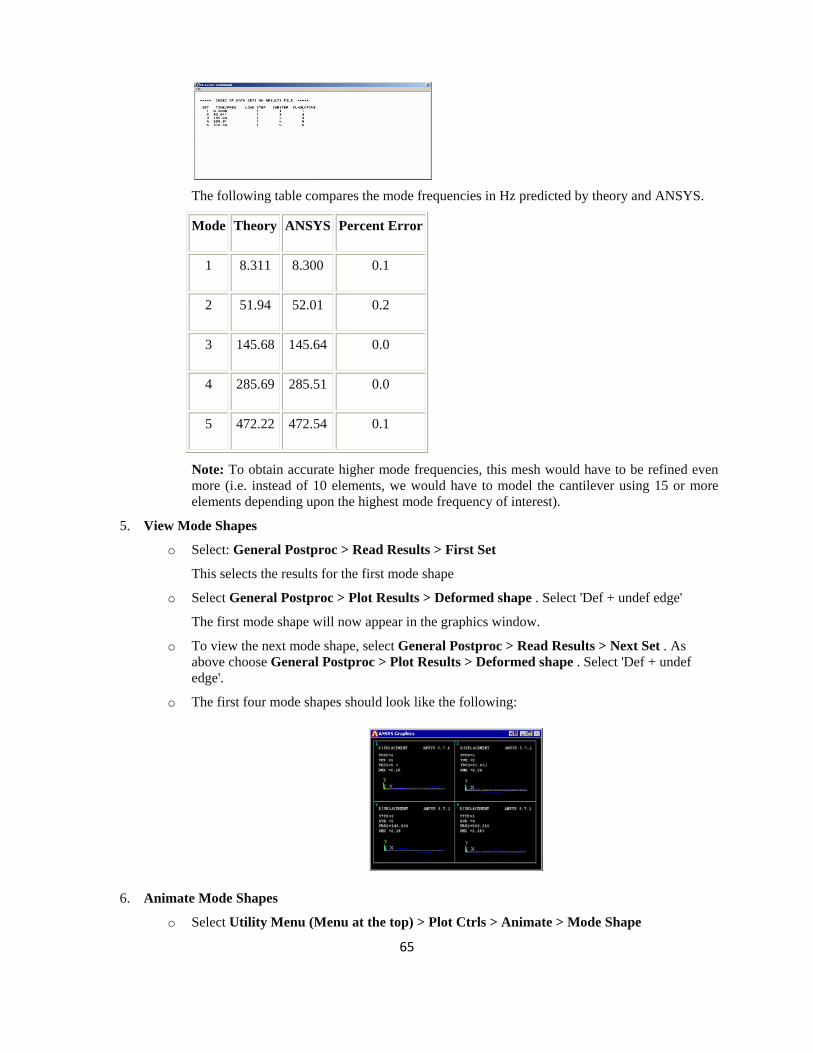
Note: To obtain accurate higher mode frequencies, this mesh would have to be refined even more (i.e. instead of 10 elements, we would have to model the cantilever using 15 or more elements depending upon the highest mode frequency of interest).
2. View Mode Shapes
o Select: General Postproc > Read Results > First Set
This selects the results for the first mode shape
o Select General Postproc > Plot Results > Deformed shape . Select 'Def + undef edge'
The first mode shape will now appear in the graphics window.
o To view the next mode shape, select General Postproc > Read Results > Next Set . As above choose General Postproc > Plot Results > Deformed shape . Select 'Def + undef edge'.
o The first four mode shapes should look like the following:
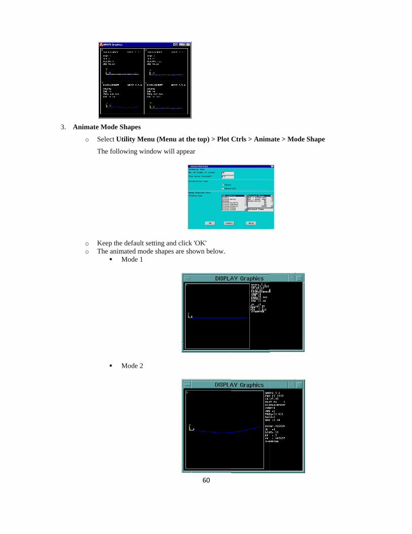
3. AAnimate Mode
o Select
The fo
o Keep to The an
e Shapes
Utility Menu
llowing windo
the default settnimated mode
Mode 1
Mode 2
u (Menu at the
ow will appea
ting and click shapes are sho
60
e top) > Plot
ar
'OK' own below.
Ctrls > Animmate > Mode S
Shape
RESULT
:
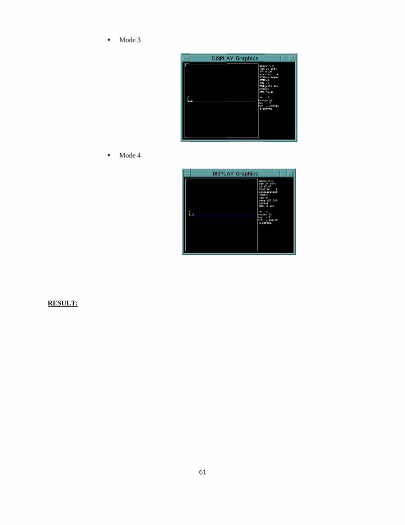
Mode 3
Mode 4
61
62
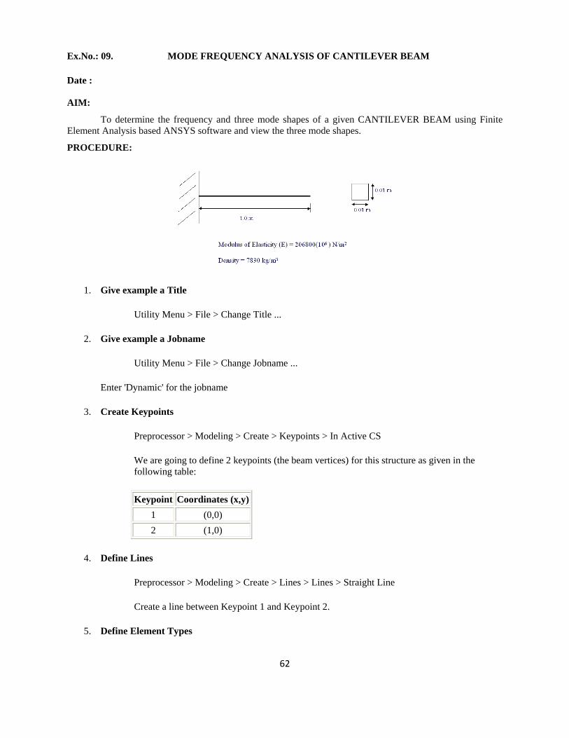
Ex.No.: 09. MODE FREQUENCY ANALYSIS OF CANTILEVER BEAM
Date :
AIM:
To determine the frequency and three mode shapes of a given CANTILEVER BEAM using Finite Element Analysis based ANSYS software and view the three mode shapes.
PROCEDURE:
1. Give example a Title
Utility Menu > File > Change Title ...
2. Give example a Jobname
Utility Menu > File > Change Jobname ...
Enter 'Dynamic' for the jobname
3. Create Keypoints
Preprocessor > Modeling > Create > Keypoints > In Active CS
We are going to define 2 keypoints (the beam vertices) for this structure as given in the following table:
Keypoint Coordinates (x,y)1 (0,0) 2 (1,0)
4. Define Lines
Preprocessor > Modeling > Create > Lines > Lines > Straight Line
Create a line between Keypoint 1 and Keypoint 2.
5. Define Element Types
63
Preprocessor > Element Type > Add/Edit/Delete...
For this problem we will use the BEAM3 (Beam 2D elastic) element. This element has 3 degrees of freedom (translation along the X and Y axis's, and rotation about the Z axis). With only 3 degrees of freedom, the BEAM3 element can only be used in 2D analysis.
6. Define Real Constants
Preprocessor > Real Constants... > Add...
In the 'Real Constants for BEAM3' window, enter the following geometric properties:
i. Cross-sectional area AREA: 0.0001 ii. Area Moment of Inertia IZZ: 8.33e-10
iii. Total beam height HEIGHT: 0.01
This defines an element with a solid rectangular cross section 0.01 m x 0.01 m.
7. Define Element Material Properties
Preprocessor > Material Props > Material Models > Structural > Linear > Elastic > Isotropic
In the window that appears, enter the following geometric properties for steel:
i. Young's modulus EX: 2.068e11 ii. Poisson's Ratio PRXY: 0.3
To enter the density of the material, double click on 'Linear' followed by 'Density' in the 'Define Material Model Behavior' Window
Enter a density of 7830
Note: For dynamic analysis, both the stiffness and the material density have to be specified.
8. Define Mesh Size
Preprocessor > Meshing > Size Cntrls > ManualSize > Lines > All Lines...
For this example we will specify 10 element divisions along the line.
9. Mesh the frame
Preprocessor > Meshing > Mesh > Lines > click 'Pick All'
Solution: Assigning Loads and Solving
5. Define Analysis Type
Solution > Analysis Type > New Analysis > Modal ANTYPE,2
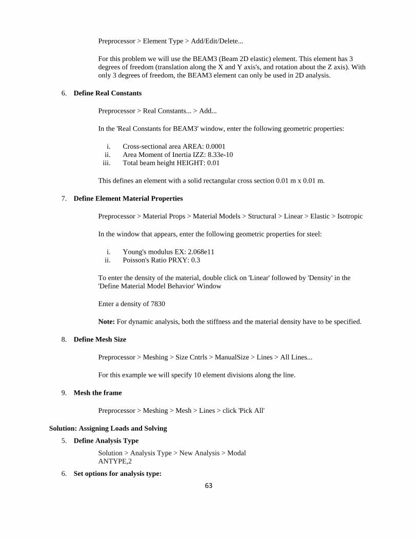
6. Set options for analysis type:
64
o Select: Solution > Analysis Type > Analysis Options.. The following window will appear
o As shown, select the Subspace method and enter 5 in the 'No. of modes to extract' o Check the box beside 'Expand mode shapes' and enter 5 in the 'No. of modes to expand' o Click 'OK'
Note that the default mode extraction method chosen is the Reduced Method. This is the fastest method as it reduces the system matrices to only consider the Master Degrees of Freedom (see below). The Subspace Method extracts modes for all DOF's. It is therefore more exact but, it also takes longer to compute (especially when the complex geometries).
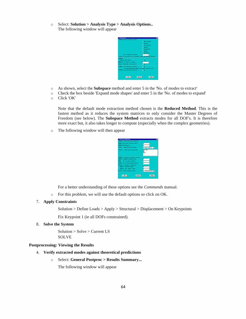
o The following window will then appear
For a better understanding of these options see the Commands manual.
o For this problem, we will use the default options so click on OK.
7. Apply Constraints
Solution > Define Loads > Apply > Structural > Displacement > On Keypoints
Fix Keypoint 1 (ie all DOFs constrained).
8. Solve the System
Solution > Solve > Current LS SOLVE
Postprocessing: Viewing the Results
4. Verify extracted modes against theoretical predictions
o Select: General Postproc > Results Summary...
The following window will appear
65
The following table compares the mode frequencies in Hz predicted by theory and ANSYS.
Mode Theory ANSYS Percent Error
1 8.311 8.300 0.1
2 51.94 52.01 0.2
3 145.68 145.64 0.0
4 285.69 285.51 0.0
5 472.22 472.54 0.1
Note: To obtain accurate higher mode frequencies, this mesh would have to be refined even more (i.e. instead of 10 elements, we would have to model the cantilever using 15 or more elements depending upon the highest mode frequency of interest).
5. View Mode Shapes
o Select: General Postproc > Read Results > First Set
This selects the results for the first mode shape
o Select General Postproc > Plot Results > Deformed shape . Select 'Def + undef edge'
The first mode shape will now appear in the graphics window.
o To view the next mode shape, select General Postproc > Read Results > Next Set . As above choose General Postproc > Plot Results > Deformed shape . Select 'Def + undef edge'.
o The first four mode shapes should look like the following:
6. Animate Mode Shapes
o Select Utility Menu (Menu at the top) > Plot Ctrls > Animate > Mode Shape
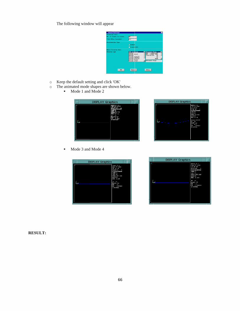
RESULT
The fo
o Keep to The an
:
llowing windo
the default settnimated mode
Mode 1 and
Mode 3 and
ow will appea
ting and click shapes are sho
d Mode 2
d Mode 4
66
ar
'OK' own below.
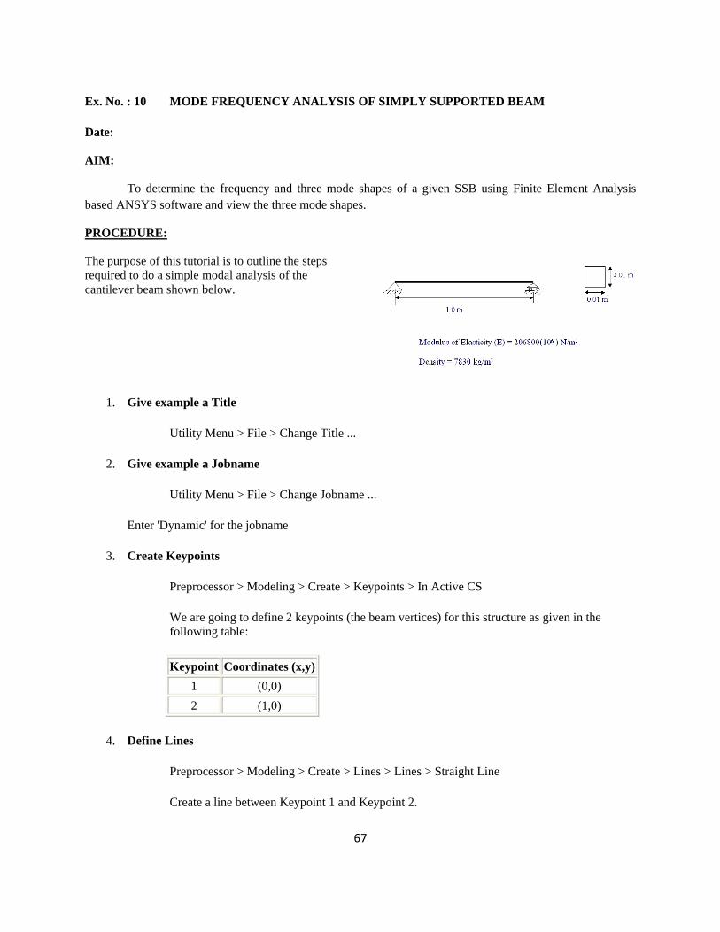
67
Ex. No. : 10 MODE FREQUENCY ANALYSIS OF SIMPLY SUPPORTED BEAM
Date:
AIM:
To determine the frequency and three mode shapes of a given SSB using Finite Element Analysis based ANSYS software and view the three mode shapes.
PROCEDURE:
The purpose of this tutorial is to outline the steps required to do a simple modal analysis of the cantilever beam shown below.
1. Give example a Title
Utility Menu > File > Change Title ...
2. Give example a Jobname
Utility Menu > File > Change Jobname ...
Enter 'Dynamic' for the jobname
3. Create Keypoints
Preprocessor > Modeling > Create > Keypoints > In Active CS
We are going to define 2 keypoints (the beam vertices) for this structure as given in the following table:
Keypoint Coordinates (x,y)1 (0,0) 2 (1,0)
4. Define Lines
Preprocessor > Modeling > Create > Lines > Lines > Straight Line
Create a line between Keypoint 1 and Keypoint 2.
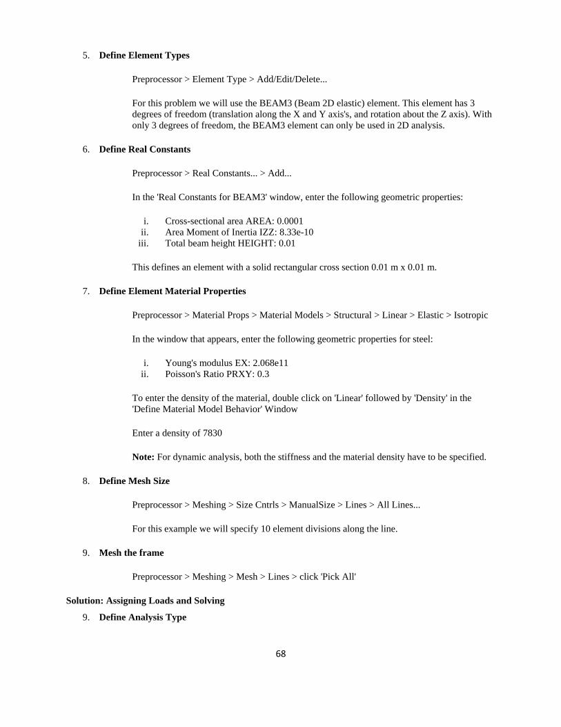
68
5. Define Element Types
Preprocessor > Element Type > Add/Edit/Delete...
For this problem we will use the BEAM3 (Beam 2D elastic) element. This element has 3 degrees of freedom (translation along the X and Y axis's, and rotation about the Z axis). With only 3 degrees of freedom, the BEAM3 element can only be used in 2D analysis.
6. Define Real Constants
Preprocessor > Real Constants... > Add...
In the 'Real Constants for BEAM3' window, enter the following geometric properties:
i. Cross-sectional area AREA: 0.0001 ii. Area Moment of Inertia IZZ: 8.33e-10
iii. Total beam height HEIGHT: 0.01
This defines an element with a solid rectangular cross section 0.01 m x 0.01 m.
7. Define Element Material Properties
Preprocessor > Material Props > Material Models > Structural > Linear > Elastic > Isotropic
In the window that appears, enter the following geometric properties for steel:
i. Young's modulus EX: 2.068e11 ii. Poisson's Ratio PRXY: 0.3
To enter the density of the material, double click on 'Linear' followed by 'Density' in the 'Define Material Model Behavior' Window
Enter a density of 7830
Note: For dynamic analysis, both the stiffness and the material density have to be specified.
8. Define Mesh Size
Preprocessor > Meshing > Size Cntrls > ManualSize > Lines > All Lines...
For this example we will specify 10 element divisions along the line.
9. Mesh the frame
Preprocessor > Meshing > Mesh > Lines > click 'Pick All'
Solution: Assigning Loads and Solving
9. Define Analysis Type
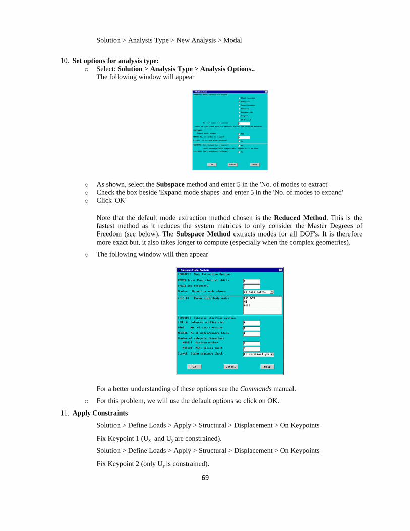
69
Solution > Analysis Type > New Analysis > Modal
10. Set options for analysis type: o Select: Solution > Analysis Type > Analysis Options..
The following window will appear
o As shown, select the Subspace method and enter 5 in the 'No. of modes to extract' o Check the box beside 'Expand mode shapes' and enter 5 in the 'No. of modes to expand' o Click 'OK'
Note that the default mode extraction method chosen is the Reduced Method. This is the fastest method as it reduces the system matrices to only consider the Master Degrees of Freedom (see below). The Subspace Method extracts modes for all DOF's. It is therefore more exact but, it also takes longer to compute (especially when the complex geometries).
o The following window will then appear
For a better understanding of these options see the Commands manual.
o For this problem, we will use the default options so click on OK.
11. Apply Constraints
Solution > Define Loads > Apply > Structural > Displacement > On Keypoints
Fix Keypoint 1 (Ux and Uy are constrained).
Solution > Define Loads > Apply > Structural > Displacement > On Keypoints
Fix Keypoint 2 (only Uy is constrained).
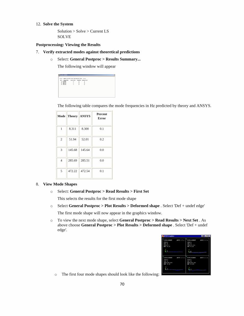
70
12. Solve the System
Solution > Solve > Current LS SOLVE
Postprocessing: Viewing the Results
7. Verify extracted modes against theoretical predictions
o Select: General Postproc > Results Summary...
The following window will appear
The following table compares the mode frequencies in Hz predicted by theory and ANSYS.
Mode Theory ANSYS Percent Error
1 8.311 8.300 0.1
2 51.94 52.01 0.2
3 145.68 145.64 0.0
4 285.69 285.51 0.0
5 472.22 472.54 0.1
8. View Mode Shapes
o Select: General Postproc > Read Results > First Set
This selects the results for the first mode shape
o Select General Postproc > Plot Results > Deformed shape . Select 'Def + undef edge'
The first mode shape will now appear in the graphics window.
o To view the next mode shape, select General Postproc > Read Results > Next Set . As above choose General Postproc > Plot Results > Deformed shape . Select 'Def + undef edge'.
o The first four mode shapes should look like the following:

9. A
RESULT
Animate Mode
o Select
The fo
o Keep to The an
:
e Shapes
Utility Menu
llowing windo
the default settnimated mode
Mode 1 and
Mode 3 and
u (Menu at the
ow will appea
ting and click shapes are sho
d Mode 2
d Mode 4
71
e top) > Plot
ar
'OK' own below.
Ctrls > Anim
mate > Mode S
Shape
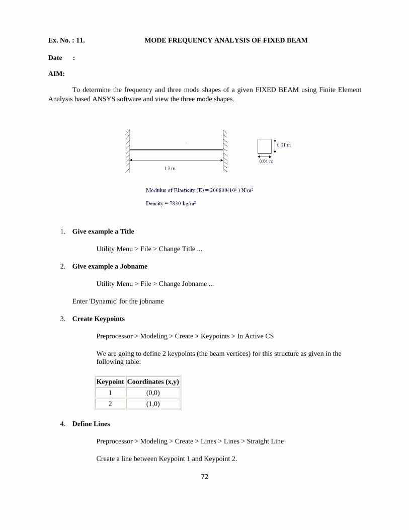
72
Ex. No. : 11. MODE FREQUENCY ANALYSIS OF FIXED BEAM
Date :
AIM:
To determine the frequency and three mode shapes of a given FIXED BEAM using Finite Element Analysis based ANSYS software and view the three mode shapes.
1. Give example a Title
Utility Menu > File > Change Title ...
2. Give example a Jobname
Utility Menu > File > Change Jobname ...
Enter 'Dynamic' for the jobname
3. Create Keypoints
Preprocessor > Modeling > Create > Keypoints > In Active CS
We are going to define 2 keypoints (the beam vertices) for this structure as given in the following table:
Keypoint Coordinates (x,y)1 (0,0) 2 (1,0)
4. Define Lines
Preprocessor > Modeling > Create > Lines > Lines > Straight Line
Create a line between Keypoint 1 and Keypoint 2.
73
5. Define Element Types
Preprocessor > Element Type > Add/Edit/Delete...
For this problem we will use the BEAM3 (Beam 2D elastic) element. This element has 3 degrees of freedom (translation along the X and Y axis's, and rotation about the Z axis). With only 3 degrees of freedom, the BEAM3 element can only be used in 2D analysis.
6. Define Real Constants
Preprocessor > Real Constants... > Add...
In the 'Real Constants for BEAM3' window, enter the following geometric properties:
i. Cross-sectional area AREA: 0.0001 ii. Area Moment of Inertia IZZ: 8.33e-10
iii. Total beam height HEIGHT: 0.01
This defines an element with a solid rectangular cross section 0.01 m x 0.01 m.
7. Define Element Material Properties
Preprocessor > Material Props > Material Models > Structural > Linear > Elastic > Isotropic
In the window that appears, enter the following geometric properties for steel:
i. Young's modulus EX: 2.068e11 ii. Poisson's Ratio PRXY: 0.3
To enter the density of the material, double click on 'Linear' followed by 'Density' in the 'Define Material Model Behavior' Window
Enter a density of 7830
Note: For dynamic analysis, both the stiffness and the material density have to be specified.
8. Define Mesh Size
Preprocessor > Meshing > Size Cntrls > ManualSize > Lines > All Lines...
For this example we will specify 10 element divisions along the line.
9. Mesh the frame
Preprocessor > Meshing > Mesh > Lines > click 'Pick All'
Solution: Assigning Loads and Solving
13. Define Analysis Type
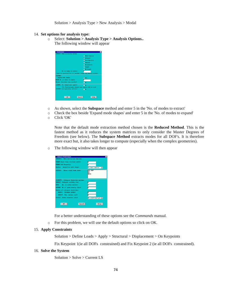
74
Solution > Analysis Type > New Analysis > Modal
14. Set options for analysis type: o Select: Solution > Analysis Type > Analysis Options..
The following window will appear
o As shown, select the Subspace method and enter 5 in the 'No. of modes to extract' o Check the box beside 'Expand mode shapes' and enter 5 in the 'No. of modes to expand' o Click 'OK'
Note that the default mode extraction method chosen is the Reduced Method. This is the fastest method as it reduces the system matrices to only consider the Master Degrees of Freedom (see below). The Subspace Method extracts modes for all DOF's. It is therefore more exact but, it also takes longer to compute (especially when the complex geometries).
o The following window will then appear
For a better understanding of these options see the Commands manual.
o For this problem, we will use the default options so click on OK.
15. Apply Constraints
Solution > Define Loads > Apply > Structural > Displacement > On Keypoints
Fix Keypoint 1(ie all DOFs constrained) and Fix Keypoint 2 (ie all DOFs constrained).
16. Solve the System
Solution > Solve > Current LS
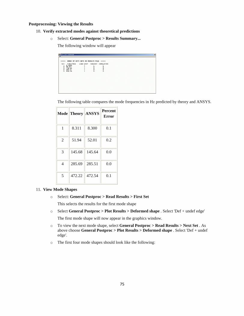
75
Postprocessing: Viewing the Results
10. Verify extracted modes against theoretical predictions
o Select: General Postproc > Results Summary...
The following window will appear
The following table compares the mode frequencies in Hz predicted by theory and ANSYS.
Mode Theory ANSYSPercent Error
1 8.311 8.300 0.1
2 51.94 52.01 0.2
3 145.68 145.64 0.0
4 285.69 285.51 0.0
5 472.22 472.54 0.1
11. View Mode Shapes
o Select: General Postproc > Read Results > First Set
This selects the results for the first mode shape
o Select General Postproc > Plot Results > Deformed shape . Select 'Def + undef edge'
The first mode shape will now appear in the graphics window.
o To view the next mode shape, select General Postproc > Read Results > Next Set . As above choose General Postproc > Plot Results > Deformed shape . Select 'Def + undef edge'.
o The first four mode shapes should look like the following:
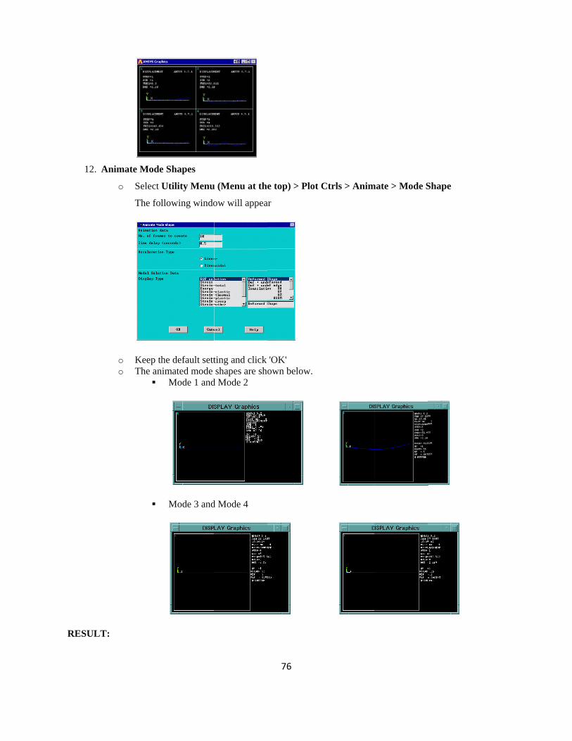
12. A
RESULT
Animate Mode
o Select
The fo
o Keep to The an
:
e Shapes
Utility Menu
llowing windo
the default settnimated mode
Mode 1 and
Mode 3 and
u (Menu at the
ow will appea
ting and click shapes are sho
d Mode 2
d Mode 4
76
e top) > Plot
ar
'OK' own below.
Ctrls > Anim
mate > Mode SShape
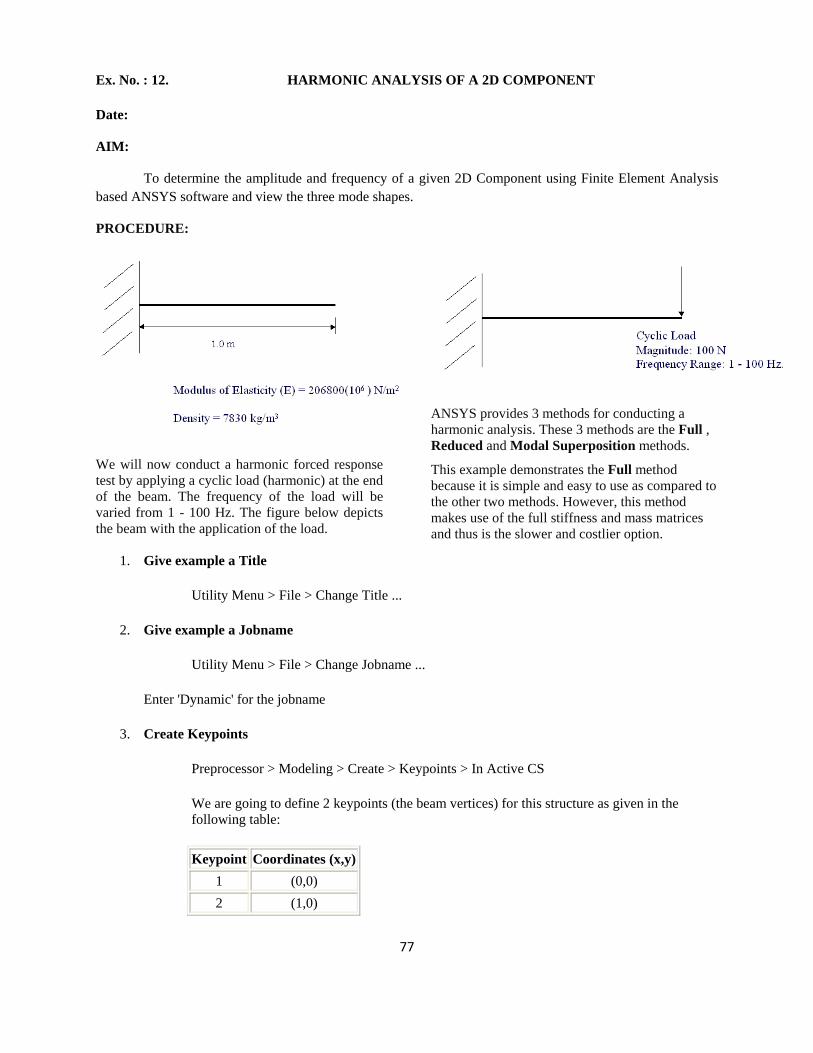
77
Ex. No. : 12. HARMONIC ANALYSIS OF A 2D COMPONENT
Date:
AIM:
To determine the amplitude and frequency of a given 2D Component using Finite Element Analysis based ANSYS software and view the three mode shapes.
PROCEDURE:
We will now conduct a harmonic forced response test by applying a cyclic load (harmonic) at the end of the beam. The frequency of the load will be varied from 1 - 100 Hz. The figure below depicts the beam with the application of the load.
ANSYS provides 3 methods for conducting a harmonic analysis. These 3 methods are the Full , Reduced and Modal Superposition methods.
This example demonstrates the Full method because it is simple and easy to use as compared to the other two methods. However, this method makes use of the full stiffness and mass matrices and thus is the slower and costlier option.
1. Give example a Title
Utility Menu > File > Change Title ...
2. Give example a Jobname
Utility Menu > File > Change Jobname ...
Enter 'Dynamic' for the jobname
3. Create Keypoints
Preprocessor > Modeling > Create > Keypoints > In Active CS
We are going to define 2 keypoints (the beam vertices) for this structure as given in the following table:
Keypoint Coordinates (x,y)1 (0,0) 2 (1,0)
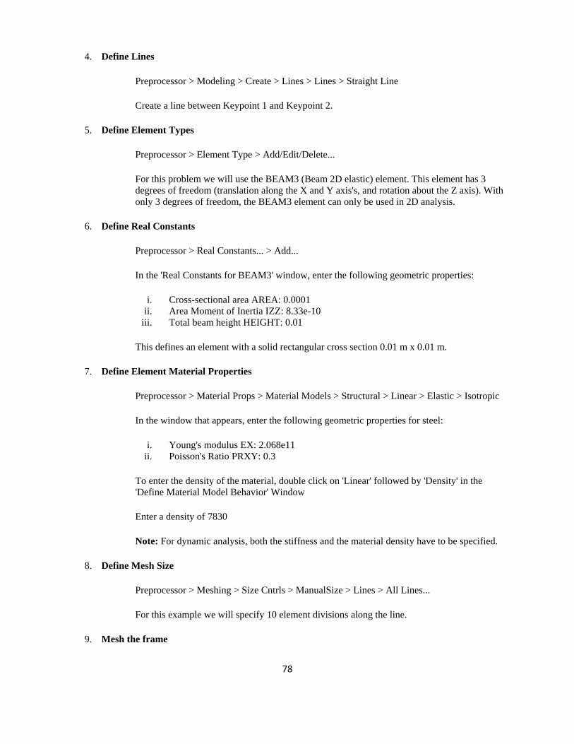
78
4. Define Lines
Preprocessor > Modeling > Create > Lines > Lines > Straight Line
Create a line between Keypoint 1 and Keypoint 2.
5. Define Element Types
Preprocessor > Element Type > Add/Edit/Delete...
For this problem we will use the BEAM3 (Beam 2D elastic) element. This element has 3 degrees of freedom (translation along the X and Y axis's, and rotation about the Z axis). With only 3 degrees of freedom, the BEAM3 element can only be used in 2D analysis.
6. Define Real Constants
Preprocessor > Real Constants... > Add...
In the 'Real Constants for BEAM3' window, enter the following geometric properties:
i. Cross-sectional area AREA: 0.0001 ii. Area Moment of Inertia IZZ: 8.33e-10
iii. Total beam height HEIGHT: 0.01
This defines an element with a solid rectangular cross section 0.01 m x 0.01 m.
7. Define Element Material Properties
Preprocessor > Material Props > Material Models > Structural > Linear > Elastic > Isotropic
In the window that appears, enter the following geometric properties for steel:
i. Young's modulus EX: 2.068e11 ii. Poisson's Ratio PRXY: 0.3
To enter the density of the material, double click on 'Linear' followed by 'Density' in the 'Define Material Model Behavior' Window
Enter a density of 7830
Note: For dynamic analysis, both the stiffness and the material density have to be specified.
8. Define Mesh Size
Preprocessor > Meshing > Size Cntrls > ManualSize > Lines > All Lines...
For this example we will specify 10 element divisions along the line.
9. Mesh the frame
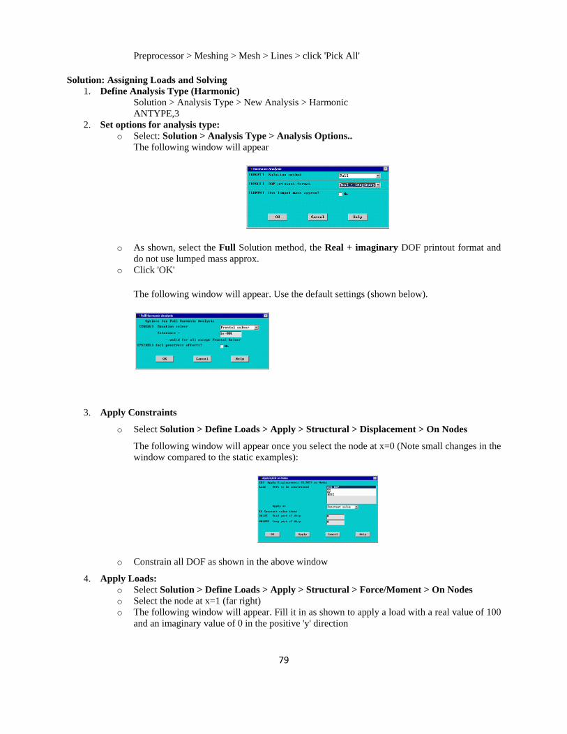
79
Preprocessor > Meshing > Mesh > Lines > click 'Pick All'
Solution: Assigning Loads and Solving 1. Define Analysis Type (Harmonic)
Solution > Analysis Type > New Analysis > Harmonic ANTYPE,3
2. Set options for analysis type: o Select: Solution > Analysis Type > Analysis Options..
The following window will appear
o As shown, select the Full Solution method, the Real + imaginary DOF printout format and do not use lumped mass approx.
o Click 'OK'
The following window will appear. Use the default settings (shown below).
3. Apply Constraints
o Select Solution > Define Loads > Apply > Structural > Displacement > On Nodes
The following window will appear once you select the node at x=0 (Note small changes in the window compared to the static examples):
o Constrain all DOF as shown in the above window
4. Apply Loads: o Select Solution > Define Loads > Apply > Structural > Force/Moment > On Nodes o Select the node at x=1 (far right) o The following window will appear. Fill it in as shown to apply a load with a real value of 100
and an imaginary value of 0 in the positive 'y' direction
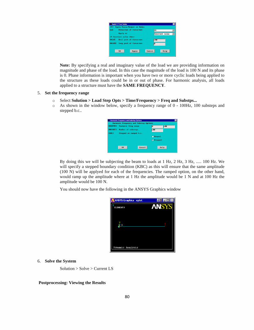
80
Note: By specifying a real and imaginary value of the load we are providing information on magnitude and phase of the load. In this case the magnitude of the load is 100 N and its phase is 0. Phase information is important when you have two or more cyclic loads being applied to the structure as these loads could be in or out of phase. For harmonic analysis, all loads applied to a structure must have the SAME FREQUENCY.
5. Set the frequency range
o Select Solution > Load Step Opts > Time/Frequency > Freq and Substps... o As shown in the window below, specify a frequency range of 0 - 100Hz, 100 substeps and
stepped b.c..
By doing this we will be subjecting the beam to loads at 1 Hz, 2 Hz, 3 Hz, ..... 100 Hz. We will specify a stepped boundary condition (KBC) as this will ensure that the same amplitude (100 N) will be applyed for each of the frequencies. The ramped option, on the other hand, would ramp up the amplitude where at 1 Hz the amplitude would be 1 N and at 100 Hz the amplitude would be 100 N.
You should now have the following in the ANSYS Graphics window
6. Solve the System
Solution > Solve > Current LS
Postprocessing: Viewing the Results
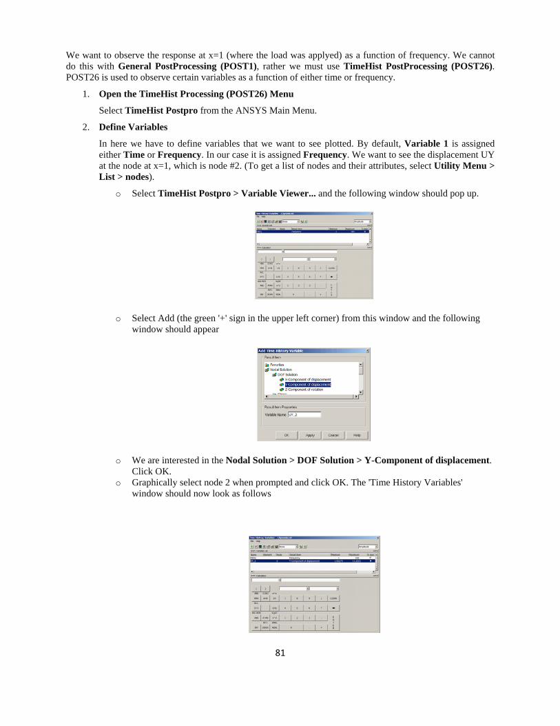
81
We want to observe the response at x=1 (where the load was applyed) as a function of frequency. We cannot do this with General PostProcessing (POST1), rather we must use TimeHist PostProcessing (POST26). POST26 is used to observe certain variables as a function of either time or frequency.
1. Open the TimeHist Processing (POST26) Menu
Select TimeHist Postpro from the ANSYS Main Menu.
2. Define Variables
In here we have to define variables that we want to see plotted. By default, Variable 1 is assigned either Time or Frequency. In our case it is assigned Frequency. We want to see the displacement UY at the node at x=1, which is node #2. (To get a list of nodes and their attributes, select Utility Menu > List > nodes).
o Select TimeHist Postpro > Variable Viewer... and the following window should pop up.
o Select Add (the green '+' sign in the upper left corner) from this window and the following window should appear
o We are interested in the Nodal Solution > DOF Solution > Y-Component of displacement. Click OK.
o Graphically select node 2 when prompted and click OK. The 'Time History Variables' window should now look as follows
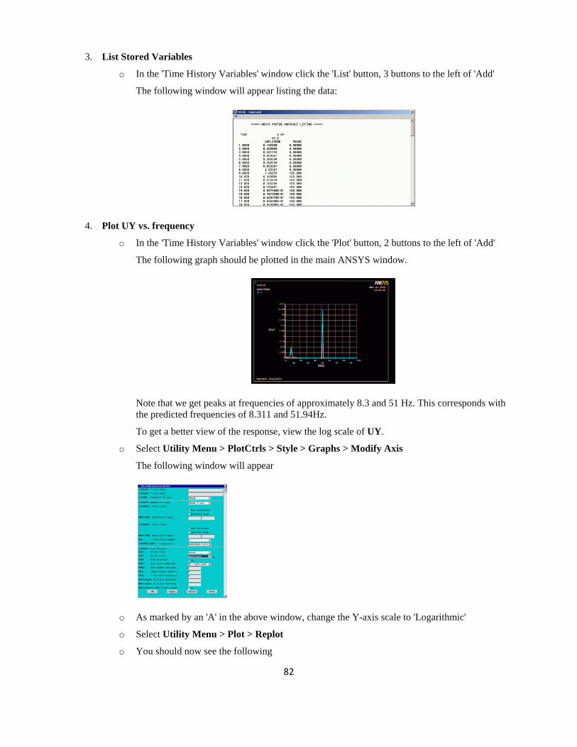
82
3. List Stored Variables
o In the 'Time History Variables' window click the 'List' button, 3 buttons to the left of 'Add'
The following window will appear listing the data:
4. Plot UY vs. frequency
o In the 'Time History Variables' window click the 'Plot' button, 2 buttons to the left of 'Add'
The following graph should be plotted in the main ANSYS window.
Note that we get peaks at frequencies of approximately 8.3 and 51 Hz. This corresponds with the predicted frequencies of 8.311 and 51.94Hz.
To get a better view of the response, view the log scale of UY.
o Select Utility Menu > PlotCtrls > Style > Graphs > Modify Axis
The following window will appear
o As marked by an 'A' in the above window, change the Y-axis scale to 'Logarithmic'
o Select Utility Menu > Plot > Replot
o You should now see the following

83
This is the response at node 2 for the cyclic load applied at this node from 0 - 100 Hz.
o For ANSYS version lower than 7.0, the 'Variable Viewer' window is not available. Use the 'Define Variables' and 'Store Data' functions under TimeHist Postpro. See the help file for instructions.
RESULT:
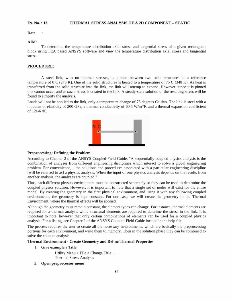
84
Ex. No. : 13. THERMAL STRESS ANALYSIS OF A 2D COMPONENT – STATIC
Date :
AIM: To determine the temperature distribution axial stress and tangential stress of a given rectangular block using FEA based ANSYS software and view the temperature distribution axial stress and tangential stress.
PROCEDURE:
A steel link, with no internal stresses, is pinned between two solid structures at a reference temperature of 0 C (273 K). One of the solid structures is heated to a temperature of 75 C (348 K). As heat is transferred from the solid structure into the link, the link will attemp to expand. However, since it is pinned this cannot occur and as such, stress is created in the link. A steady-state solution of the resulting stress will be found to simplify the analysis. Loads will not be applied to the link, only a temperature change of 75 degrees Celsius. The link is steel with a modulus of elasticity of 200 GPa, a thermal conductivity of 60.5 W/m*K and a thermal expansion coefficient of 12e-6 /K.
Preprocessing: Defining the Problem According to Chapter 2 of the ANSYS Coupled-Field Guide, "A sequentially coupled physics analysis is the combination of analyses from different engineering disciplines which interact to solve a global engineering problem. For convenience, ...the solutions and procedures associated with a particular engineering discipline [will be referred to as] a physics analysis. When the input of one physics analysis depends on the results from another analysis, the analyses are coupled." Thus, each different physics environment must be constructed seperately so they can be used to determine the coupled physics solution. However, it is important to note that a single set of nodes will exist for the entire model. By creating the geometry in the first physical environment, and using it with any following coupled environments, the geometry is kept constant. For our case, we will create the geometry in the Thermal Environment, where the thermal effects will be applied. Although the geometry must remain constant, the element types can change. For instance, thermal elements are required for a thermal analysis while structural elements are required to deterime the stress in the link. It is important to note, however that only certain combinations of elements can be used for a coupled physics analysis. For a listing, see Chapter 2 of the ANSYS Coupled-Field Guide located in the help file. The process requires the user to create all the necessary environments, which are basically the preprocessing portions for each environment, and write them to memory. Then in the solution phase they can be combined to solve the coupled analysis. Thermal Environment - Create Geometry and Define Thermal Properties
1. Give example a Title Utility Menu > File > Change Title ... Thermal Stress Analysis
2. Open preprocessor menu
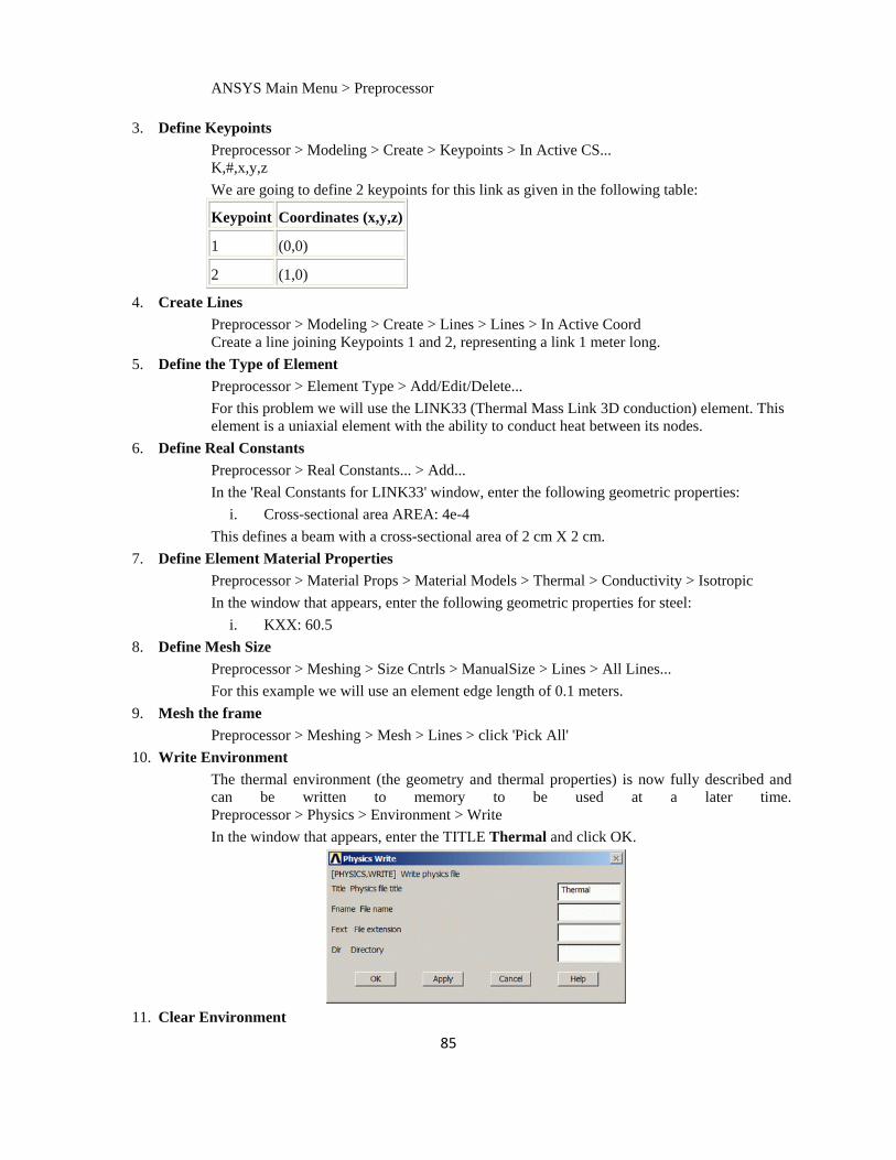
85
ANSYS Main Menu > Preprocessor
3. Define Keypoints Preprocessor > Modeling > Create > Keypoints > In Active CS... K,#,x,y,z We are going to define 2 keypoints for this link as given in the following table:
Keypoint Coordinates (x,y,z)
1 (0,0)
2 (1,0)
4. Create Lines Preprocessor > Modeling > Create > Lines > Lines > In Active Coord Create a line joining Keypoints 1 and 2, representing a link 1 meter long.
5. Define the Type of Element Preprocessor > Element Type > Add/Edit/Delete... For this problem we will use the LINK33 (Thermal Mass Link 3D conduction) element. This element is a uniaxial element with the ability to conduct heat between its nodes.
6. Define Real Constants Preprocessor > Real Constants... > Add... In the 'Real Constants for LINK33' window, enter the following geometric properties:
i. Cross-sectional area AREA: 4e-4 This defines a beam with a cross-sectional area of 2 cm X 2 cm.
7. Define Element Material Properties Preprocessor > Material Props > Material Models > Thermal > Conductivity > Isotropic In the window that appears, enter the following geometric properties for steel:
i. KXX: 60.5 8. Define Mesh Size
Preprocessor > Meshing > Size Cntrls > ManualSize > Lines > All Lines... For this example we will use an element edge length of 0.1 meters.
9. Mesh the frame Preprocessor > Meshing > Mesh > Lines > click 'Pick All'
10. Write Environment The thermal environment (the geometry and thermal properties) is now fully described and can be written to memory to be used at a later time. Preprocessor > Physics > Environment > Write In the window that appears, enter the TITLE Thermal and click OK.
11. Clear Environment
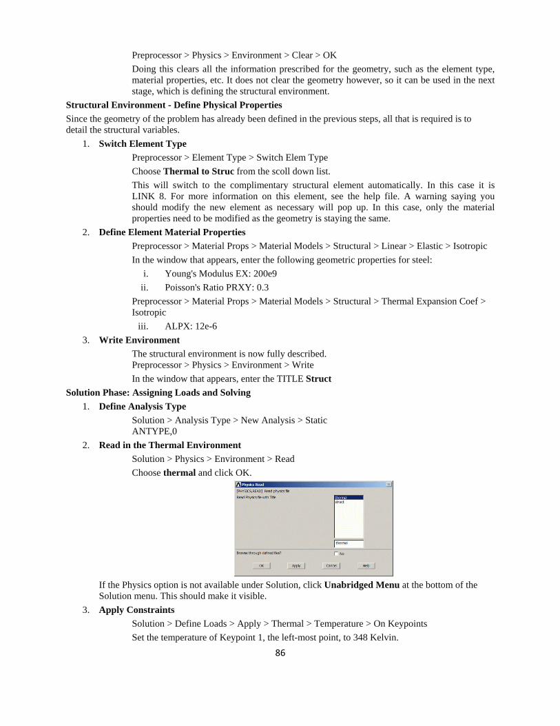
86
Preprocessor > Physics > Environment > Clear > OK Doing this clears all the information prescribed for the geometry, such as the element type, material properties, etc. It does not clear the geometry however, so it can be used in the next stage, which is defining the structural environment.
Structural Environment - Define Physical Properties Since the geometry of the problem has already been defined in the previous steps, all that is required is to detail the structural variables.
1. Switch Element Type Preprocessor > Element Type > Switch Elem Type Choose Thermal to Struc from the scoll down list. This will switch to the complimentary structural element automatically. In this case it is LINK 8. For more information on this element, see the help file. A warning saying you should modify the new element as necessary will pop up. In this case, only the material properties need to be modified as the geometry is staying the same.
2. Define Element Material Properties Preprocessor > Material Props > Material Models > Structural > Linear > Elastic > Isotropic In the window that appears, enter the following geometric properties for steel:
i. Young's Modulus EX: 200e9 ii. Poisson's Ratio PRXY: 0.3
Preprocessor > Material Props > Material Models > Structural > Thermal Expansion Coef > Isotropic
iii. ALPX: 12e-6 3. Write Environment
The structural environment is now fully described. Preprocessor > Physics > Environment > Write In the window that appears, enter the TITLE Struct
Solution Phase: Assigning Loads and Solving 1. Define Analysis Type
Solution > Analysis Type > New Analysis > Static ANTYPE,0
2. Read in the Thermal Environment Solution > Physics > Environment > Read Choose thermal and click OK.
If the Physics option is not available under Solution, click Unabridged Menu at the bottom of the Solution menu. This should make it visible.
3. Apply Constraints Solution > Define Loads > Apply > Thermal > Temperature > On Keypoints Set the temperature of Keypoint 1, the left-most point, to 348 Kelvin.
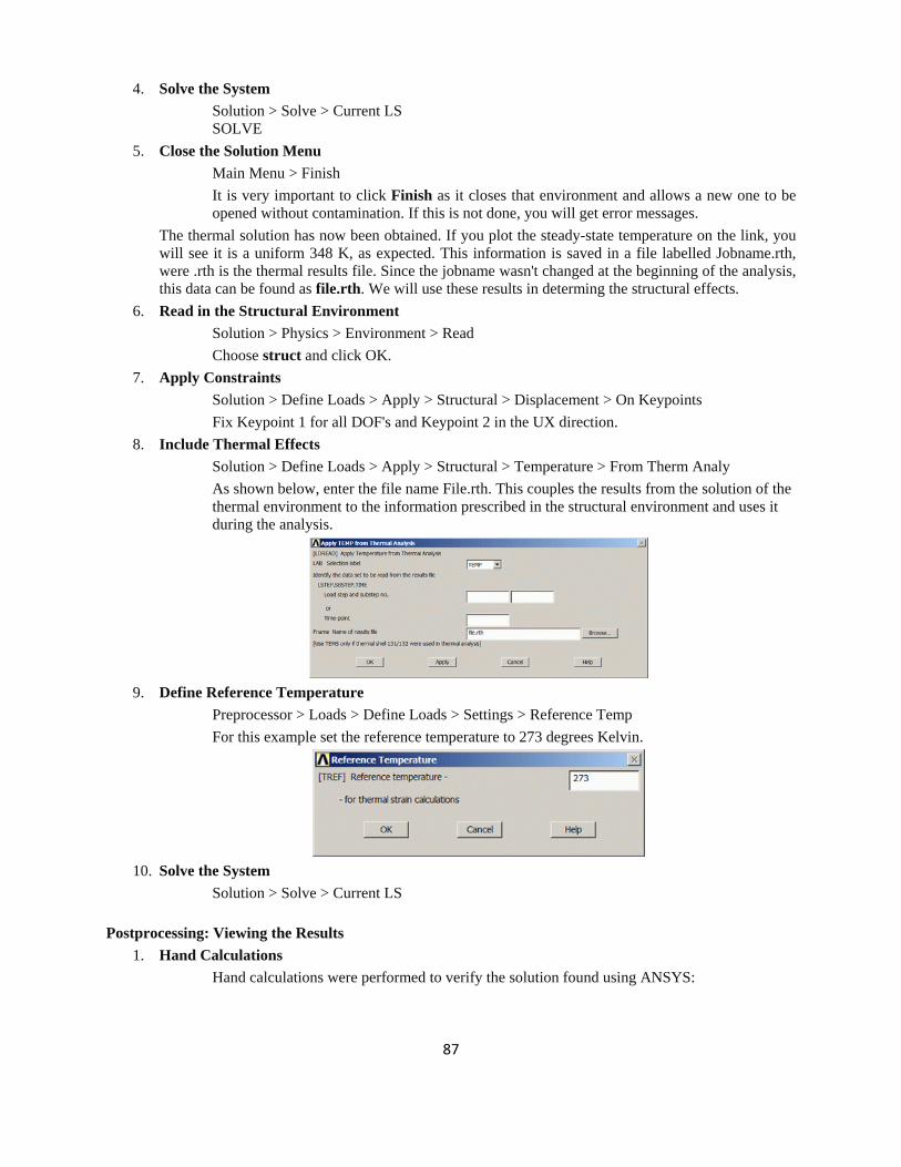
87
4. Solve the System Solution > Solve > Current LS SOLVE
5. Close the Solution Menu Main Menu > Finish It is very important to click Finish as it closes that environment and allows a new one to be opened without contamination. If this is not done, you will get error messages.
The thermal solution has now been obtained. If you plot the steady-state temperature on the link, you will see it is a uniform 348 K, as expected. This information is saved in a file labelled Jobname.rth, were .rth is the thermal results file. Since the jobname wasn't changed at the beginning of the analysis, this data can be found as file.rth. We will use these results in determing the structural effects.
6. Read in the Structural Environment Solution > Physics > Environment > Read Choose struct and click OK.
7. Apply Constraints Solution > Define Loads > Apply > Structural > Displacement > On Keypoints Fix Keypoint 1 for all DOF's and Keypoint 2 in the UX direction.
8. Include Thermal Effects Solution > Define Loads > Apply > Structural > Temperature > From Therm Analy As shown below, enter the file name File.rth. This couples the results from the solution of the thermal environment to the information prescribed in the structural environment and uses it during the analysis.
9. Define Reference Temperature
Preprocessor > Loads > Define Loads > Settings > Reference Temp For this example set the reference temperature to 273 degrees Kelvin.
10. Solve the System
Solution > Solve > Current LS
Postprocessing: Viewing the Results 1. Hand Calculations
Hand calculations were performed to verify the solution found using ANSYS:
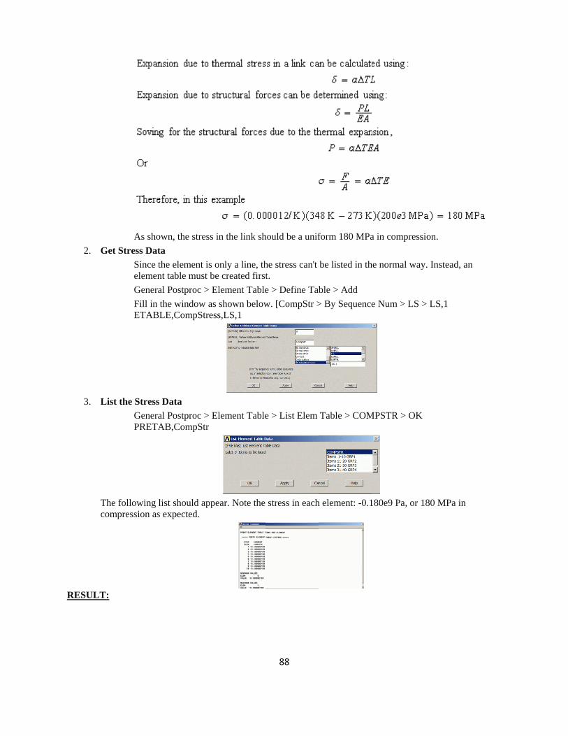
2. G
3. L
Tco
RESULT
As shoGet Stress Dat
Since telemenGeneraFill in ETAB
List the StressGeneraPRETA
he following lompression as
:
own, the stressta the element is nt table must bal Postproc > Ethe window aLE,CompStre
Data al Postproc > EAB,CompStr
list should apps expected.
s in the link sh
only a line, thbe created firstElement Tables shown below
ess,LS,1
Element Table
pear. Note the
88
hould be a unif
he stress can't t. e > Define Tabw. [CompStr >
e > List Elem
stress in each
form 180 MPa
be listed in th
ble > Add > By Sequence
Table > COM
h element: -0.1
a in compressi
he normal way
e Num > LS >
MPSTR > OK
180e9 Pa, or 1
ion.
y. Instead, an
> LS,1
80 MPa in

89
Ex. No. : 14. CONDUCTIVE HEAT TRANSFER ANALYSIS OF A 2D COMPONENT
Date:
AIM: To determine the temperature distribution and heat flux of a given 2D component using FEA based ANSYS software and view the temperature and heat flux.
PROCEDURE:
The Simple Conduction Example is constrained as shown in the following figure. Thermal conductivity (k) of the material is 10 W/m*C and the block is assumed to be infinitely long.
Preprocessing: Defining the Problem
1. Give example a Title 2. Open preprocessor menu
ANSYS Main Menu > Preprocessor
3. Create geometry Preprocessor > Modeling > Create > Areas > Rectangle > By 2 Corners > X=0, Y=0, Width=1, Height=1
4. Define the Type of Element Preprocessor > Element Type > Add/Edit/Delete... > click 'Add' > Select Thermal Mass Solid, Quad 4Node 55
For this example, we will use PLANE55 (Thermal Solid, Quad 4node 55). This element has 4 nodes and a single DOF (temperature) at each node. PLANE55 can only be used for 2 dimensional steady-state or transient thermal analysis.
5. Element Material Properties Preprocessor > Material Props > Material Models > Thermal > Conductivity > Isotropic > KXX = 10 (Thermal conductivity)
6. Mesh Size Preprocessor > Meshing > Size Cntrls > ManualSize > Areas > All Areas > 0.05
7. Mesh Preprocessor > Meshing > Mesh > Areas > Free > Pick All
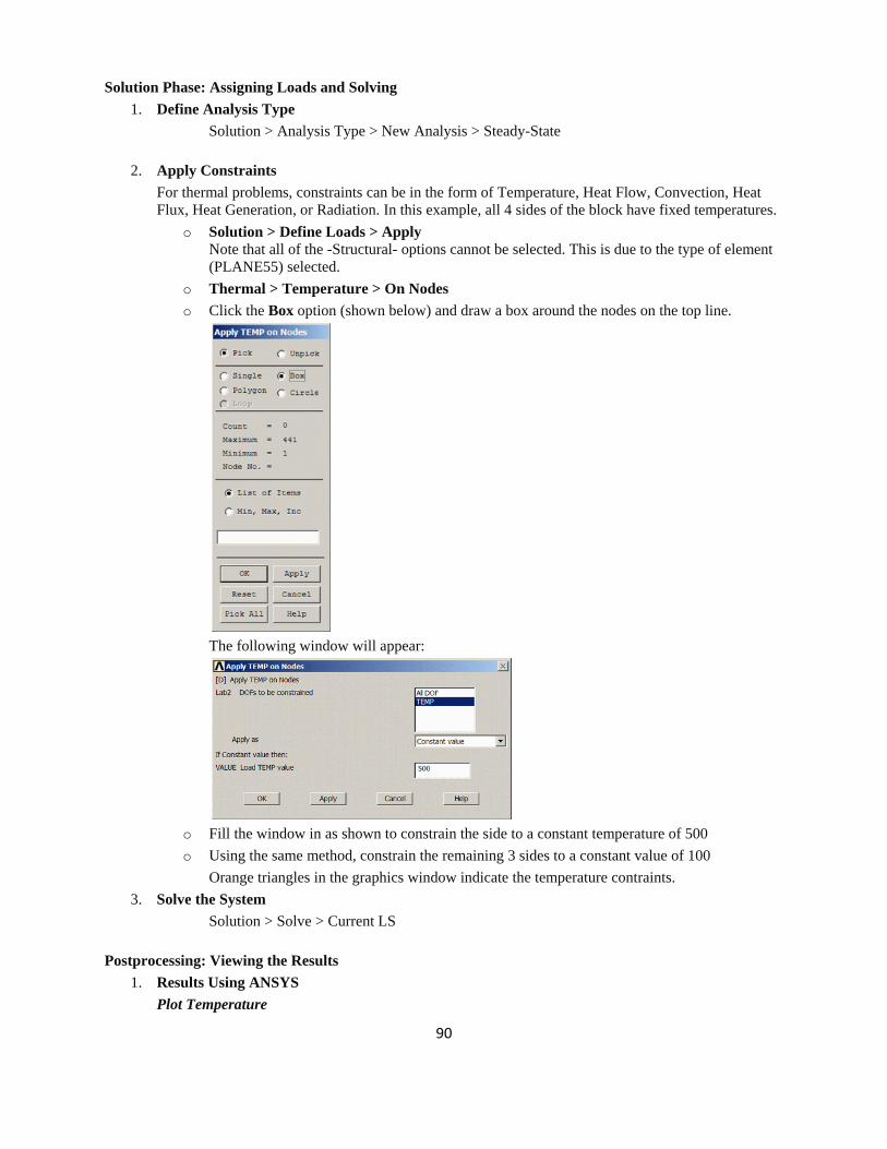
90
Solution Phase: Assigning Loads and Solving 1. Define Analysis Type
Solution > Analysis Type > New Analysis > Steady-State
2. Apply Constraints For thermal problems, constraints can be in the form of Temperature, Heat Flow, Convection, Heat Flux, Heat Generation, or Radiation. In this example, all 4 sides of the block have fixed temperatures.
o Solution > Define Loads > Apply Note that all of the -Structural- options cannot be selected. This is due to the type of element (PLANE55) selected.
o Thermal > Temperature > On Nodes o Click the Box option (shown below) and draw a box around the nodes on the top line.
The following window will appear:
o Fill the window in as shown to constrain the side to a constant temperature of 500 o Using the same method, constrain the remaining 3 sides to a constant value of 100
Orange triangles in the graphics window indicate the temperature contraints. 3. Solve the System
Solution > Solve > Current LS
Postprocessing: Viewing the Results 1. Results Using ANSYS
Plot Temperature
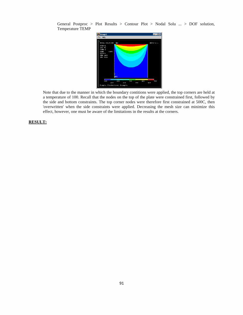
91
General Postproc > Plot Results > Contour Plot > Nodal Solu ... > DOF solution, Temperature TEMP
Note that due to the manner in which the boundary contitions were applied, the top corners are held at a temperature of 100. Recall that the nodes on the top of the plate were constrained first, followed by the side and bottom constraints. The top corner nodes were therefore first constrained at 500C, then 'overwritten' when the side constraints were applied. Decreasing the mesh size can minimize this effect, however, one must be aware of the limitations in the results at the corners.
RESULT:
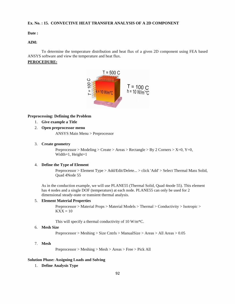
92
Ex. No. : 15. CONVECTIVE HEAT TRANSFER ANALYSIS OF A 2D COMPONENT
Date :
AIM:
To determine the temperature distribution and heat flux of a given 2D component using FEA based ANSYS software and view the temperature and heat flux. PEROCEDURE:
Preprocessing: Defining the Problem 1. Give example a Title 2. Open preprocessor menu
ANSYS Main Menu > Preprocessor
3. Create geometry Preprocessor > Modeling > Create > Areas > Rectangle > By 2 Corners > X=0, Y=0, Width=1, Height=1
4. Define the Type of Element Preprocessor > Element Type > Add/Edit/Delete... > click 'Add' > Select Thermal Mass Solid, Quad 4Node 55
As in the conduction example, we will use PLANE55 (Thermal Solid, Quad 4node 55). This element has 4 nodes and a single DOF (temperature) at each node. PLANE55 can only be used for 2 dimensional steady-state or transient thermal analysis.
5. Element Material Properties Preprocessor > Material Props > Material Models > Thermal > Conductivity > Isotropic > KXX = 10 This will specify a thermal conductivity of 10 W/m*C.
6. Mesh Size Preprocessor > Meshing > Size Cntrls > ManualSize > Areas > All Areas > 0.05
7. Mesh Preprocessor > Meshing > Mesh > Areas > Free > Pick All
Solution Phase: Assigning Loads and Solving 1. Define Analysis Type
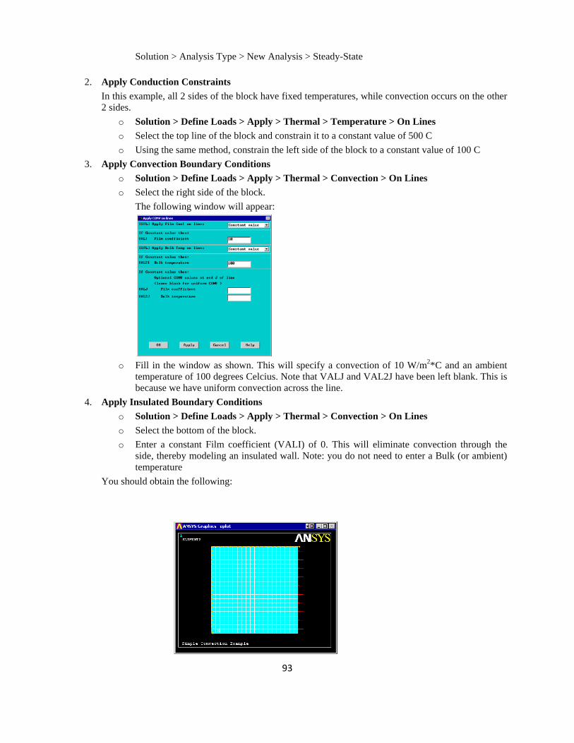
93
Solution > Analysis Type > New Analysis > Steady-State
2. Apply Conduction Constraints In this example, all 2 sides of the block have fixed temperatures, while convection occurs on the other 2 sides.
o Solution > Define Loads > Apply > Thermal > Temperature > On Lines o Select the top line of the block and constrain it to a constant value of 500 C o Using the same method, constrain the left side of the block to a constant value of 100 C
3. Apply Convection Boundary Conditions o Solution > Define Loads > Apply > Thermal > Convection > On Lines o Select the right side of the block.
The following window will appear:
o Fill in the window as shown. This will specify a convection of 10 W/m2*C and an ambient
temperature of 100 degrees Celcius. Note that VALJ and VAL2J have been left blank. This is because we have uniform convection across the line.
4. Apply Insulated Boundary Conditions o Solution > Define Loads > Apply > Thermal > Convection > On Lines o Select the bottom of the block. o Enter a constant Film coefficient (VALI) of 0. This will eliminate convection through the
side, thereby modeling an insulated wall. Note: you do not need to enter a Bulk (or ambient) temperature
You should obtain the following:
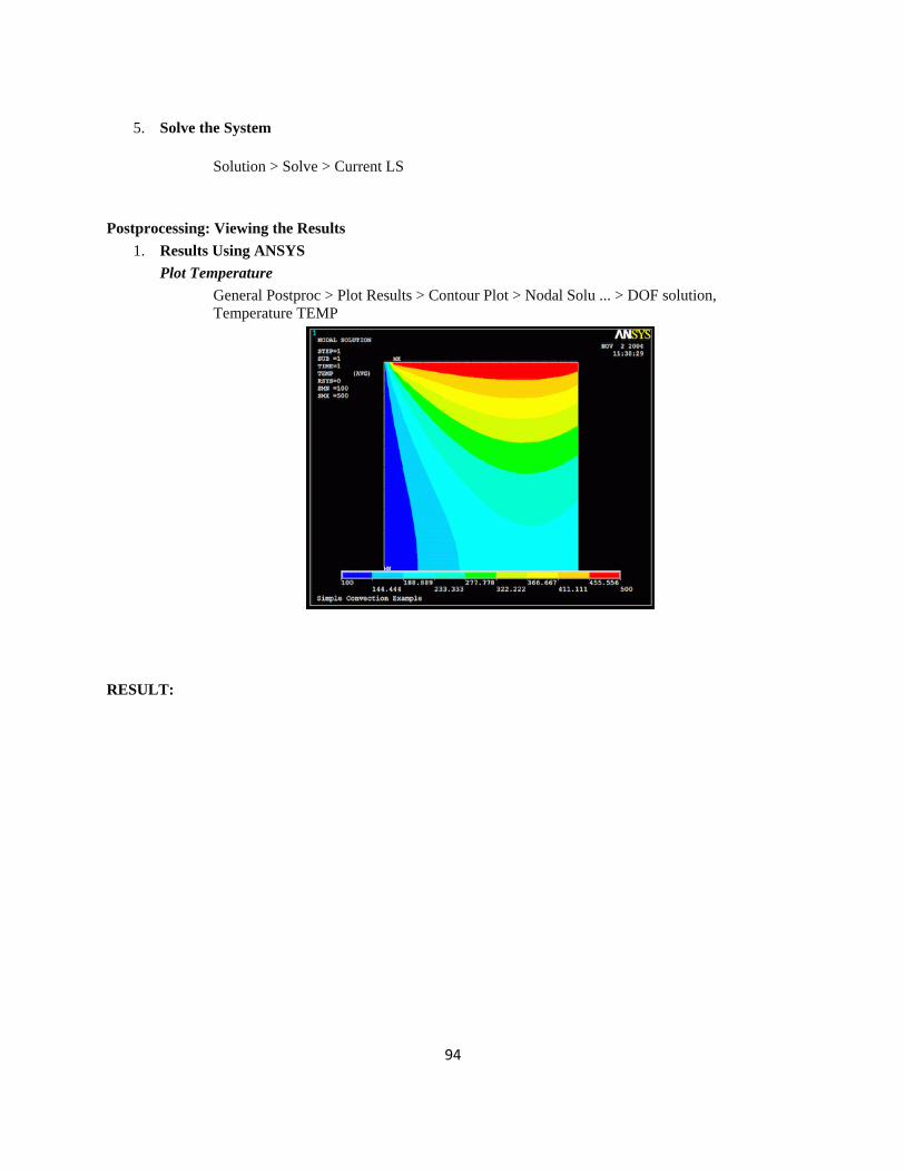
94
5. Solve the System
Solution > Solve > Current LS
Postprocessing: Viewing the Results 1. Results Using ANSYS
Plot Temperature General Postproc > Plot Results > Contour Plot > Nodal Solu ... > DOF solution, Temperature TEMP
RESULT:
Related Documents