Answers to Warm-Up Exercises

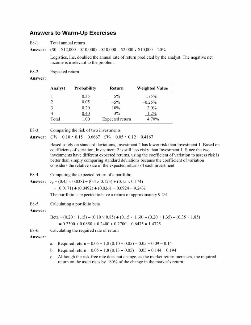
Answers to Warm-Up Exercises

E8-1. Total annual return

Answer: ($0 $12,000 $10,000) $10,000 $2,000 $10,000 20%

Logistics, Inc. doubled the annual rate of return predicted by the analyst. The negative net

income is irrelevant to the problem.

E8-2. Expected return

Answer:

Analyst Probability Return Weighted Value

1 0.35 5% 1.75%

2 0.05 5% 0.25%

3 0.20 10% 2.0%

4 0.40 3% 1.2%

Total 1.00 Expected return 4.70%

E8-3. Comparing the risk of two investments

Answer: CV1 0.10 0.15 0.6667 CV2 0.05 0.12 0.4167

Based solely on standard deviations, Investment 2 has lower risk than Investment 1. Based on

coefficients of variation, Investment 2 is still less risky than Investment 1. Since the two

investments have different expected returns, using the coefficient of variation to assess risk is

better than simply comparing standard deviations because the coefficient of variation

considers the relative size of the expected returns of each investment.

E8-4. Computing the expected return of a portfolio

Answer: rp (0.45 0.038) (0.4 0.123) (0.15 0.174)

(0.0171) (0.0492) (0.0261 0.0924 9.24%

The portfolio is expected to have a return of approximately 9.2%.

E8-5. Calculating a portfolio beta

Answer:

Beta (0.20 1.15) (0.10 0.85) (0.15 1.60) (0.20 1.35) (0.35 1.85)

0.2300 0.0850 0.2400 0.2700 0.6475 1.4725

E8-6. Calculating the required rate of return

Answer:

a. Required return 0.05 1.8 (0.10 0.05) 0.05 0.09 0.14

b. Required return 0.05 1.8 (0.13 0.05) 0.05 0.144 0.194

c. Although the risk-free rate does not change, as the market return increases, the required

return on the asset rises by 180% of the change in the market’s return.

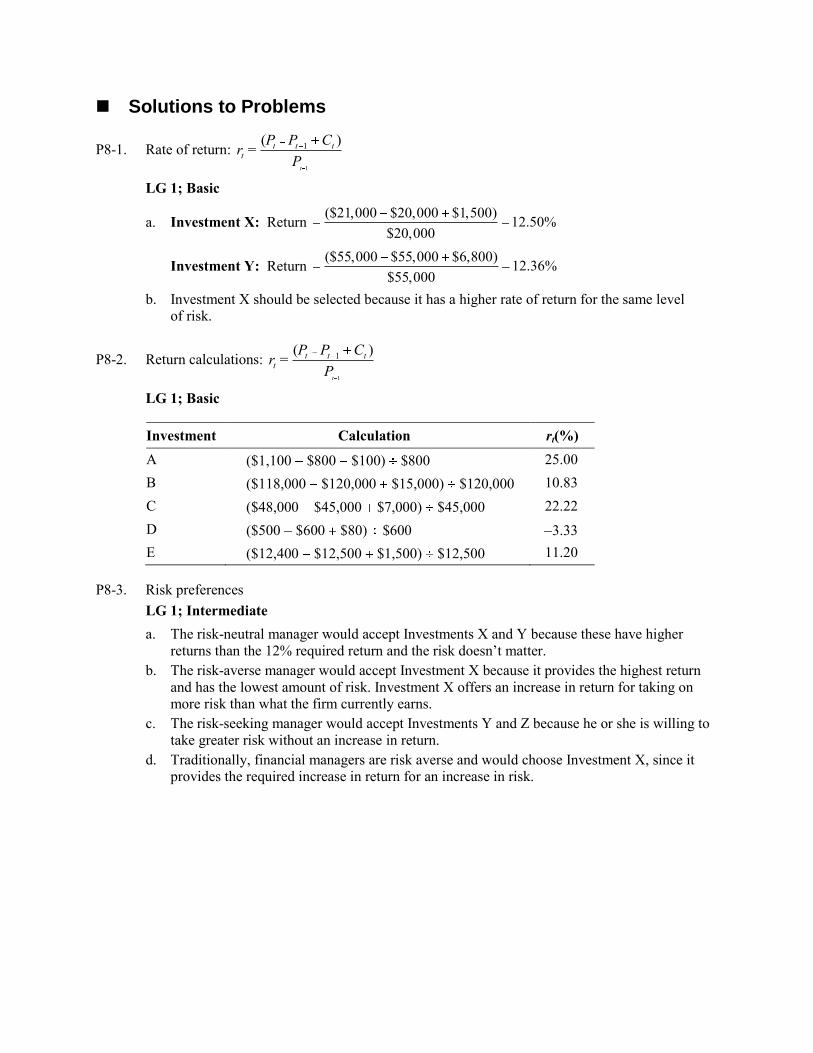
Solutions to Problems

P8-1. Rate of return: 1

1( )

t

t t t

t

P P Cr =

P

LG 1; Basic

a. Investment X: Return ($21,000 $20,000 $1,500)

12.50%$20,000

Investment Y: Return ($55,000 $55,000 $6,800)

12.36%$55,000

b. Investment X should be selected because it has a higher rate of return for the same level of risk.

P8-2. Return calculations: 1

1( )

t

t t t

t

P P Cr =

P

LG 1; Basic

Investment Calculation rt(%)

A ($1,100 $800 $100) $800 25.00

B ($118,000 $120,000 $15,000) $120,000 10.83

C ($48,000 $45,000 $7,000) $45,000 22.22

D ($500 $600 $80) $600 3.33

E ($12,400 $12,500 $1,500) $12,500 11.20

P8-3. Risk preferences

LG 1; Intermediate

a. The risk-neutral manager would accept Investments X and Y because these have higher

returns than the 12% required return and the risk doesn’t matter.

b. The risk-averse manager would accept Investment X because it provides the highest return

and has the lowest amount of risk. Investment X offers an increase in return for taking on more risk than what the firm currently earns.

c. The risk-seeking manager would accept Investments Y and Z because he or she is willing to

take greater risk without an increase in return.

d. Traditionally, financial managers are risk averse and would choose Investment X, since it provides the required increase in return for an increase in risk.

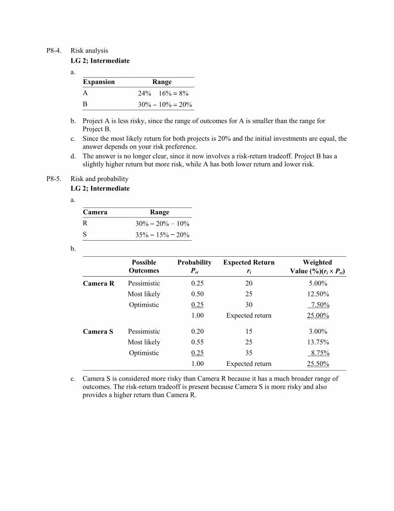
P8-4. Risk analysis

LG 2; Intermediate

a.

Expansion Range

A 24% 16% 8%

B 30% 10% 20%

b. Project A is less risky, since the range of outcomes for A is smaller than the range for

Project B.

c. Since the most likely return for both projects is 20% and the initial investments are equal, the answer depends on your risk preference.

d. The answer is no longer clear, since it now involves a risk-return tradeoff. Project B has a slightly higher return but more risk, while A has both lower return and lower risk.

P8-5. Risk and probability

LG 2; Intermediate

a.

Camera Range

R 30% 20% 10%

S 35% 15% 20%

b.

Possible

Outcomes

Probability

Pri

Expected Return

ri

Weighted

Value (%)(ri Pri)

Camera R Pessimistic 0.25 20 5.00%

Most likely 0.50 25 12.50%

Optimistic 0.25 30 7.50%

1.00 Expected return 25.00%

Camera S Pessimistic 0.20 15 3.00%

Most likely 0.55 25 13.75%

Optimistic 0.25 35 8.75%

1.00 Expected return 25.50%

c. Camera S is considered more risky than Camera R because it has a much broader range of

outcomes. The risk-return tradeoff is present because Camera S is more risky and also

provides a higher return than Camera R.

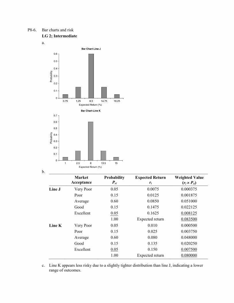
P8-6. Bar charts and risk

LG 2; Intermediate

a.

b.

Market

Acceptance

Probability

Pri

Expected Return

ri

Weighted Value

(ri Pri)

Line J Very Poor 0.05 0.0075 0.000375

Poor 0.15 0.0125 0.001875

Average 0.60 0.0850 0.051000

Good 0.15 0.1475 0.022125

Excellent 0.05 0.1625 0.008125

1.00 Expected return 0.083500

Line K Very Poor 0.05 0.010 0.000500

Poor 0.15 0.025 0.003750

Average 0.60 0.080 0.048000

Good 0.15 0.135 0.020250

Excellent 0.05 0.150 0.007500

1.00 Expected return 0.080000

c. Line K appears less risky due to a slightly tighter distribution than line J, indicating a lower

range of outcomes.

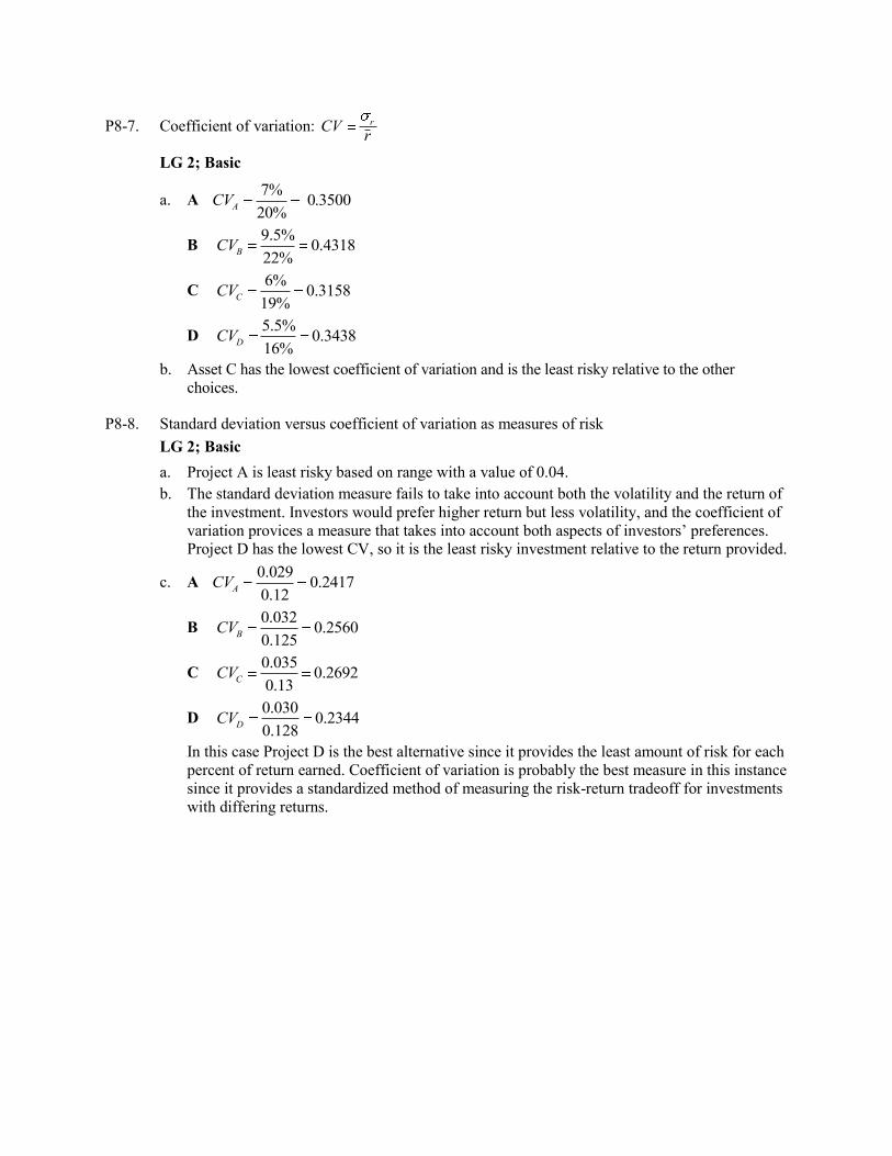
P8-7. Coefficient of variation: rCVr

LG 2; Basic

a. A 7%

0.350020%

ACV

B 9.5%

0.431822%

BCV

C 6%

0.315819%

CCV

D 5.5%

0.343816%

DCV

b. Asset C has the lowest coefficient of variation and is the least risky relative to the other

choices.

P8-8. Standard deviation versus coefficient of variation as measures of risk

LG 2; Basic

a. Project A is least risky based on range with a value of 0.04.

b. The standard deviation measure fails to take into account both the volatility and the return of

the investment. Investors would prefer higher return but less volatility, and the coefficient of

variation provices a measure that takes into account both aspects of investors’ preferences. Project D has the lowest CV, so it is the least risky investment relative to the return provided.

c. A 0.029

0.24170.12

ACV

B 0.032

0.25600.125

BCV

C 0.035

0.26920.13

CCV

D 0.030

0.23440.128

DCV

In this case Project D is the best alternative since it provides the least amount of risk for each

percent of return earned. Coefficient of variation is probably the best measure in this instance

since it provides a standardized method of measuring the risk-return tradeoff for investments

with differing returns.

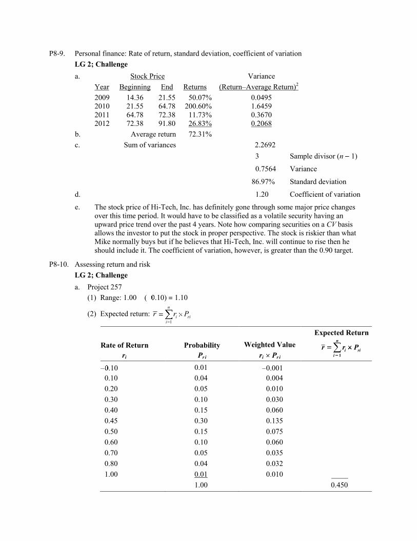
P8-9. Personal finance: Rate of return, standard deviation, coefficient of variation

LG 2; Challenge

a. Stock Price Variance

Year Beginning End Returns (Return–Average Return)2

2009

2010

2011

2012

14.36

21.55

64.78

72.38

21.55

64.78

72.38

91.80

50.07%

200.60%

11.73%

26.83%

0.0495

1.6459

0.3670

0.2068

b. Average return 72.31%

c. Sum of variances 2.2692

3 Sample divisor (n 1)

0.7564 Variance

86.97% Standard deviation

d. 1.20 Coefficient of variation

e. The stock price of Hi-Tech, Inc. has definitely gone through some major price changes

over this time period. It would have to be classified as a volatile security having an

upward price trend over the past 4 years. Note how comparing securities on a CV basis

allows the investor to put the stock in proper perspective. The stock is riskier than what

Mike normally buys but if he believes that Hi-Tech, Inc. will continue to rise then he

should include it. The coefficient of variation, however, is greater than the 0.90 target.

P8-10. Assessing return and risk

LG 2; Challenge

a. Project 257

(1) Range: 1.00 ( .10) 1.10

(2) Expected return: =1

n

i ri

i

r r P

Rate of Return

ri

Probability

Pr i

Weighted Value

ri Pr i

Expected Return

1

n

i ri

i

r r P

.10 0.01 0.001

0.10 0.04 0.004

0.20 0.05 0.010

0.30 0.10 0.030

0.40 0.15 0.060

0.45 0.30 0.135

0.50 0.15 0.075

0.60 0.10 0.060

0.70 0.05 0.035

0.80 0.04 0.032

1.00 0.01 0.010

1.00 0.450

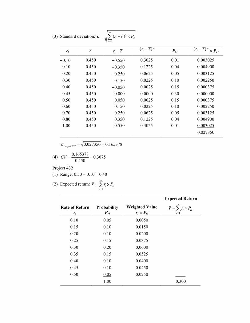
(3) Standard deviation: 2

1

( )n

i ri

i

r r P

ri r ir r

( )ir r 2

Pr i ( )ir r 2

Pr i

0.10 0.450 0.550 0.3025 0.01 0.003025

0.10 0.450 0.350 0.1225 0.04 0.004900

0.20 0.450 0.250 0.0625 0.05 0.003125

0.30 0.450 0.150 0.0225 0.10 0.002250

0.40 0.450 0.050 0.0025 0.15 0.000375

0.45 0.450 0.000 0.0000 0.30 0.000000

0.50 0.450 0.050 0.0025 0.15 0.000375

0.60 0.450 0.150 0.0225 0.10 0.002250

0.70 0.450 0.250 0.0625 0.05 0.003125

0.80 0.450 0.350 0.1225 0.04 0.004900

1.00 0.450 0.550 0.3025 0.01 0.003025

0.027350

Project 2570.027350 0.165378

(4) 0.165378

0.36750.450

CV

Project 432

(1) Range: 0.50 0.10 0.40

(2) Expected return: 1

n

i ri

i

r r P

Rate of Return

ri

Probability

Pr i

Weighted Value

ri Pri

Expected Return

=1

n

i ri

i

r r P

0.10 0.05 0.0050

0.15 0.10 0.0150

0.20 0.10 0.0200

0.25 0.15 0.0375

0.30 0.20 0.0600

0.35 0.15 0.0525

0.40 0.10 0.0400

0.45 0.10 0.0450

0.50 0.05 0.0250

1.00 0.300

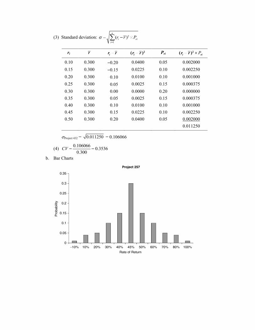
(3) Standard deviation: 2

1

( )n

i ri

i

r r P

ri r ir r 2( )

ir r Pri P2( )

i rir r

0.10 0.300 0.20 0.0400 0.05 0.002000

0.15 0.300 0.15 0.0225 0.10 0.002250

0.20 0.300 0.10 0.0100 0.10 0.001000

0.25 0.300 0.05 0.0025 0.15 0.000375

0.30 0.300 0.00 0.0000 0.20 0.000000

0.35 0.300 0.05 0.0025 0.15 0.000375

0.40 0.300 0.10 0.0100 0.10 0.001000

0.45 0.300 0.15 0.0225 0.10 0.002250

0.50 0.300 0.20 0.0400 0.05 0.002000

0.011250

Project 432 0.011250 0.106066

(4) 0.106066

0.35360.300

CV

b. Bar Charts

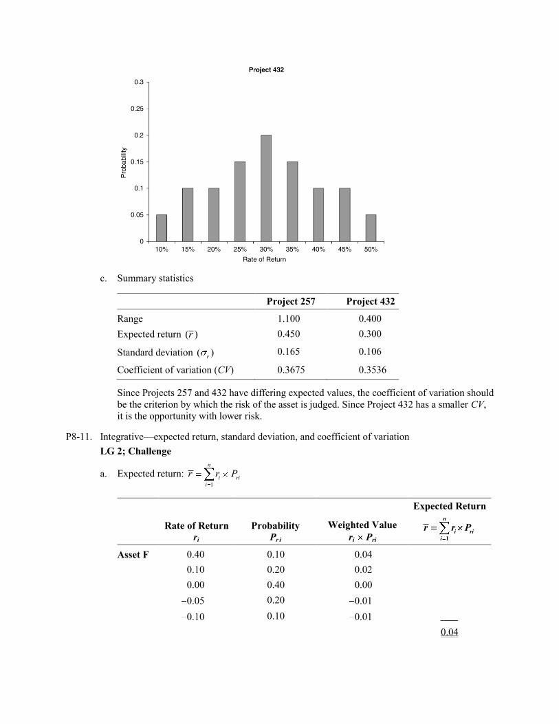
c. Summary statistics

Project 257 Project 432

Range 1.100 0.400

Expected return ( )r 0.450 0.300

Standard deviation ( )r

0.165 0.106

Coefficient of variation (CV) 0.3675 0.3536

Since Projects 257 and 432 have differing expected values, the coefficient of variation should

be the criterion by which the risk of the asset is judged. Since Project 432 has a smaller CV,

it is the opportunity with lower risk.

P8-11. Integrative—expected return, standard deviation, and coefficient of variation

LG 2; Challenge

a. Expected return: 1

n

i ri

i

r r P

Rate of Return

ri

Probability

Pr i

Weighted Value

ri Pri

Expected Return

1

n

i ri

i

r r P

Asset F 0.40 0.10 0.04

0.10 0.20 0.02

0.00 0.40 0.00

0.05 0.20 0.01

0.10 0.10 0.01

0.04

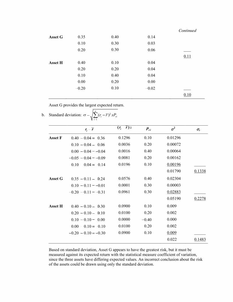
Continued

Asset G 0.35 0.40 0.14

0.10 0.30 0.03

0.20 0.30 0.06

0.11

Asset H 0.40 0.10 0.04

0.20 0.20 0.04

0.10 0.40 0.04

0.00 0.20 0.00

0.20 0.10 0.02

0.10

Asset G provides the largest expected return.

b. Standard deviation: 2

1

( )n

i ri

i

r r xP

ir r

( )ir r 2

Pr i 2 r

Asset F 0.40 0.04 0.36 0.1296 0.10 0.01296

0.10 0.04 0.06 0.0036 0.20 0.00072

0.00 0.04 0.04 0.0016 0.40 0.00064

0.05 0.04 0.09 0.0081 0.20 0.00162

0.10 0.04 0.14 0.0196 0.10 0.00196

0.01790 0.1338

Asset G 0.35 0.11 .24 0.0576 0.40 0.02304

0.10 0.11 0.01 0.0001 0.30 0.00003

0.20 0.11 0.31 0.0961 0.30 0.02883

0.05190 0.2278

Asset H 0.40 0.10 .30 0.0900 0.10 0.009

0.20 0.10 .10 0.0100 0.20 0.002

0.10 0.10 0.00 0.0000 0.40 0.000

0.00 0.10 0.10 0.0100 0.20 0.002

0.20 0.10 0.30 0.0900 0.10 0.009

0.022 0.1483

Based on standard deviation, Asset G appears to have the greatest risk, but it must be

measured against its expected return with the statistical measure coefficient of variation,

since the three assets have differing expected values. An incorrect conclusion about the risk

of the assets could be drawn using only the standard deviation.

c. standard deviation ( )

Coefficient of variation =expected value

Asset F: 0.1338

3.3450.04

CV

Asset G: 0.2278

2.0710.11

CV

Asset H: 0.1483

1.4830.10

CV

As measured by the coefficient of variation, Asset F has the largest relative risk.

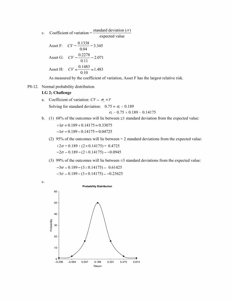
P8-12. Normal probability distribution

LG 2; Challenge

a. Coefficient of variation: CV rr

Solving for standard deviation: 0.75 r 0.189

r 0.75 0.189 0.14175

b. (1) 68% of the outcomes will lie between 1 standard deviation from the expected value:

1 0.189 0.14175 0.33075

1 0.189 0.14175 0.04725

(2) 95% of the outcomes will lie between 2 standard deviations from the expected value:

2 0.189 (2 0.14175) 0.4725

2 0.189 (2 0.14175) 0.0945

(3) 99% of the outcomes will lie between 3 standard deviations from the expected value:

3 0.189 (3 0.14175) 0.61425

3 0.189 (3 0.14175) 0.23625

c.

P8-13. Personal finance: Portfolio return and standard deviation

LG 3; Challenge

a. Expected portfolio return for each year: rp (wL rL) (wM rM)

Year

Asset L

(wL rL)

Asset M

(wM rM)

Expected

Portfolio Return

rp

2013 (14% 0.40 5.6%) (20% 0.60 12.0%) 17.6%

2014 (14% 0.40 5.6%) (18% 0.60 10.8%) 16.4%

2015 (16% 0.40 6.4%) (16% 0.60 9.6%) 16.0%

2016 (17% 0.40 6.8%) (14% 0.60 8.4%) 15.2%

2017 (17% 0.40 6.8%) (12% 0.60 7.2%) 14.0%

2018 (19% 0.40 7.6%) (10% 0.60 6.0%) 13.6%

b. Portfolio return: 1

n

j j

j

p

w r

rn

17.6 16.4 16.0 15.2 14.0 13.6

15.467 15.5%6

pr

c. Standard deviation: 2

1

( )

( 1)

ni

rp

i

r r

n

2 2 2

2 2 2

(17.6% 15.5%) (16.4% 15.5%) (16.0% 15.5%)

(15.2% 15.5%) (14.0% 15.5%) (13.6% 15.5%)

6 1rp

2 2 2

2 2 2

(2.1%) (0.9%) (0.5%)

( 0.3%) ( 1.5%) ( 1.9%)

5rp

(.000441 0.000081 0.000025 0.000009 0.000225 0.000361)

5rp

0.001142

0.000228% 0.0151 1.51%5

rp

d. The assets are negatively correlated.

e. Combining these two negatively correlated assets reduces overall portfolio risk.

P8-14. Portfolio analysis

LG 3; Challenge

a. Expected portfolio return:

Alternative 1: 100% Asset F

16% 17% 18% 19%17.5%

4pr

Alternative 2: 50% Asset F 50% Asset G

Year Asset F

(wF rF)

Asset G

(wG rG)

Portfolio Return

rp

2013 (16% 0.50 8.0%) (17% 0.50 8.5%) 16.5%

2014 (17% 0.50 8.5%) (16% 0.50 8.0%) 16.5%

2015 (18% 0.50 9.0%) (15% 0.50 7.5%) 16.5%

2016 (19% 0.50 9.5%) (14% 0.50 7.0%) 16.5%

16.5% 16.5% 16.5% 16.5%16.5%

4pr

Alternative 3: 50% Asset F 50% Asset H

Year Asset F

(wF rF)

Asset H

(wH rH)

Portfolio Return

rp

2013 (16% 0.50 8.0%) (14% 0.50 7.0%) 15.0%

2014 (17% 0.50 8.5%) (15% 0.50 7.5%) 16.0%

2015 (18% 0.50 9.0%) (16% 0.50 8.0%) 17.0%

2016 (19% 0.50 9.5%) (17% 0.50 8.5%) 18.0%

15.0% 16.0% 17.0% 18.0%16.5%

4pr

b. Standard deviation: 2

1

( )

( 1)

ni

rp

i

r r

n

(1)

2 2 2 2[(16.0% 17.5%) (17.0% 17.5%) (18.0% 17.5%) (19.0% 17.5%) ]

4 1F

2 2 2 2[( 1.5%) ( 0.5%) (0.5%) (1.5%) ]

3F

(0.000225 0.000025 0.000025 0.000225)

3F

0.0005

.000167 0.01291 1.291%3

F

(2)

2 2 2 2[(16.5% 16.5%) (16.5% 16.5%) (16.5% 16.5%) (16.5% 16.5%) ]

4 1FG

2 2 2 2[(0) (0) (0) (0) ]

3FG

0FG

(3)

2 2 2 2[(15.0% 16.5%) (16.0% 16.5%) (17.0% 16.5%) (18.0% 16.5%) ]

4 1FH

2 2 2 2[( 1.5%) ( 0.5%) (0.5%) (1.5%) ]

3FH

[(0.000225 0.000025 0.000025 0.000225)]

3FH

0.0005

0.000167 0.012910 1.291%3

FH

c. Coefficient of variation: CV rr

1.291%0.0738

17.5%F

CV

00

16.5%FG

CV

1.291%0.0782

16.5%FH

CV

d. Summary:

rp: Expected Value

of Portfolio rp CVp

Alternative 1 (F) 17.5% 1.291% 0.0738

Alternative 2 (FG) 16.5% 0 0.0

Alternative 3 (FH) 16.5% 1.291% 0.0782

Since the assets have different expected returns, the coefficient of variation should be used to

determine the best portfolio. Alternative 3, with positively correlated assets, has the highest

coefficient of variation and therefore is the riskiest. Alternative 2 is the best choice; it is perfectly negatively correlated and therefore has the lowest coefficient of variation.

P8-15. Correlation, risk, and return

LG 4; Intermediate

a. (1) Range of expected return: between 8% and 13%

(2) Range of the risk: between 5% and 10%

b. (1) Range of expected return: between 8% and 13%

(2) Range of the risk: 0 risk 10%

c. (1) Range of expected return: between 8% and 13%

(2) Range of the risk: 0 risk 10%

P8-16. Personal finance: International investment returns

LG 1, 4; Intermediate

a. Returnpesos 24,750 20,500 4,250

0.20732 20.73%20,500 20,500

b. Price in pesos 20.50

Purchase price $2.22584 1,000 shares $2,225.84Pesos per dollar 9.21

Price in pesos 24.75

Sales price $2.51269 1,000 shares $2,512.69Pesos per dollar 9.85

c. Returnpesos 2,512.69 2,225.84 286.85

0.12887 12.89%2,225.84 2,225.84

d. The two returns differ due to the change in the exchange rate between the peso and the

dollar. The peso had depreciation (and thus the dollar appreciated) between the purchase date

and

the sale date, causing a decrease in total return. The answer in part c is the more important of the two returns for Joe. An investor in foreign securities will carry exchange-rate risk.

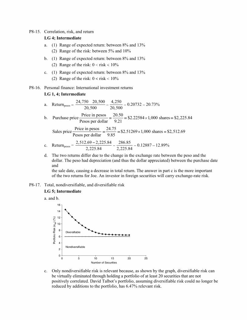
P8-17. Total, nondiversifiable, and diversifiable risk

LG 5; Intermediate

a. and b.

c. Only nondiversifiable risk is relevant because, as shown by the graph, diversifiable risk can

be virtually eliminated through holding a portfolio of at least 20 securities that are not

positively correlated. David Talbot’s portfolio, assuming diversifiable risk could no longer be reduced by additions to the portfolio, has 6.47% relevant risk.

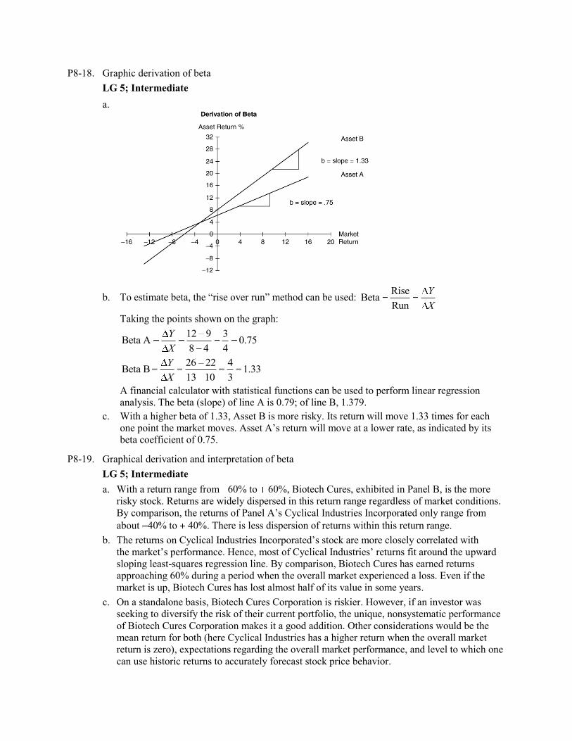
P8-18. Graphic derivation of beta

LG 5; Intermediate

a.

b. To estimate beta, the ―rise over run‖ method can be used: Rise

BetaRun

Y

X

Taking the points shown on the graph:

12 9 3Beta A 0.75

8 4 4

Y

X

26 22 4Beta B 1.33

13 10 3

Y

X

A financial calculator with statistical functions can be used to perform linear regression

analysis. The beta (slope) of line A is 0.79; of line B, 1.379.

c. With a higher beta of 1.33, Asset B is more risky. Its return will move 1.33 times for each

one point the market moves. Asset A’s return will move at a lower rate, as indicated by its beta coefficient of 0.75.

P8-19. Graphical derivation and interpretation of beta

LG 5; Intermediate

a. With a return range from 60% to 60%, Biotech Cures, exhibited in Panel B, is the more

risky stock. Returns are widely dispersed in this return range regardless of market conditions.

By comparison, the returns of Panel A’s Cyclical Industries Incorporated only range from

about 40% to 40%. There is less dispersion of returns within this return range.

b. The returns on Cyclical Industries Incorporated’s stock are more closely correlated with

the market’s performance. Hence, most of Cyclical Industries’ returns fit around the upward

sloping least-squares regression line. By comparison, Biotech Cures has earned returns

approaching 60% during a period when the overall market experienced a loss. Even if the

market is up, Biotech Cures has lost almost half of its value in some years.

c. On a standalone basis, Biotech Cures Corporation is riskier. However, if an investor was

seeking to diversify the risk of their current portfolio, the unique, nonsystematic performance

of Biotech Cures Corporation makes it a good addition. Other considerations would be the

mean return for both (here Cyclical Industries has a higher return when the overall market

return is zero), expectations regarding the overall market performance, and level to which one

can use historic returns to accurately forecast stock price behavior.

P8-20. Interpreting beta

LG 5; Basic

Effect of change in market return on asset with beta of 1.20:

a. 1.20 (15%) 18.0% increase

b. 1.20 ( 8%) 9.6% decrease

c. 1.20 (0%) no change

d. The asset is more risky than the market portfolio, which has a beta of 1. The higher beta

makes the return move more than the market.

P8-21. Betas

LG 5; Basic

a. and b.

Asset

Beta

Increase in

Market Return

Expected Impact

on Asset Return

Decrease in

Market Return

Impact on

Asset Return

A 0.50 0.10 0.05 0.10 0.05

B 1.60 0.10 0.16 0.10 0.16

C 0.20 0.10 0.02 0.10 0.02

D 0.90 0.10 0.09 0.10 0.09

c. Asset B should be chosen because it will have the highest increase in return.

d. Asset C would be the appropriate choice because it is a defensive asset, moving in opposition to the market. In an economic downturn, Asset C’s return is increasing.

P8-22. Personal finance: Betas and risk rankings

LG 5; Intermediate

a.

Stock Beta

Most risky B 1.40

A 0.80

Least risky C 0.30

b. and c.

Asset

Beta Increase in

Market Return

Expected Impact

on Asset Return

Decrease in

Market Return

Impact on

Asset Return

A 0.80 0.12 0.096 0.05 0.04

B 1.40 0.12 0.168 0.05 0.07

C 0.30 0.12 0.036 0.05 0.015

d. In a declining market, an investor would choose the defensive stock, Stock C. While the

market declines, the return on C increases.

e. In a rising market, an investor would choose Stock B, the aggressive stock. As the market rises one point, Stock B rises 1.40 points.

P8-23. Personal finance: Portfolio betas: bp 1

n

j j

j

w b

LG 5; Intermediate

a.

Portfolio A Portfolio B

Asset Beta wA wA bA wB wB bB

1 1.30 0.10 0.130 0.30 0.39

2 0.70 0.30 0.210 0.10 0.07

3 1.25 0.10 0.125 0.20 0.25

4 1.10 0.10 0.110 0.20 0.22

5 0.90 0.40 0.360 0.20 0.18

bA 0.935 bB 1.11

b. Portfolio A is slightly less risky than the market (average risk), while Portfolio B is more

risky than the market. Portfolio B’s return will move more than Portfolio A’s for a given

increase or decrease in market return. Portfolio B is the more risky.

P8-24. Capital asset pricing model (CAPM): rj RF [bj (rm RF)]

LG 6; Basic

Case rj RF [bj (rm RF)]

A 8.9% 5% [1.30 (8% 5%)]

B 12.5% 8% [0.90 (13% 8%)]

C 8.4% 9% [ 0.20 (12% 9%)]

D 15.0% 10% [1.00 (15% 10%)]

E 8.4% 6% [0.60 (10% 6%)]

P8-25. Personal finance: Beta coefficients and the capital asset pricing model

LG 5, 6; Intermediate

To solve this problem you must take the CAPM and solve for beta. The resulting model is:

Beta F

m F

r R

r R

a. 10% 5% 5%

Beta 0.454516% 5% 11%

b. 15% 5% 10%

Beta 0.909116% 5% 11%

c. 18% 5% 13%

Beta 1.181816% 5% 11%

d. 20% 5% 15%

Beta 1.363616% 5% 11%

e. If Katherine is willing to take a maximum of average risk then she will be able to have an

expected return of only 16%. (r 5% 1.0(16% 5%) 16%.)

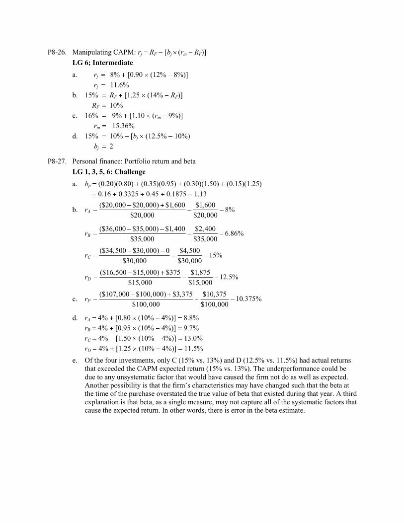
P8-26. Manipulating CAPM: rj RF [bj (rm RF)]

LG 6; Intermediate

a. rj 8% [0.90 (12% 8%)]

rj 11.6%

b. 15% RF [1.25 (14% RF)]

RF 10%

c. 16% 9% [1.10 (rm 9%)]

rm 15.36%

d. 15% 10% [bj (12.5% 10%)

bj 2

P8-27. Personal finance: Portfolio return and beta

LG 1, 3, 5, 6: Challenge

a. bp (0.20)(0.80) (0.35)(0.95) (0.30)(1.50) (0.15)(1.25)

0.16 0.3325 0.45 0.1875 1.13

b. rA ($20,000 $20,000) $1,600 $1,600

8%$20,000 $20,000

rB ($36,000 $35,000) $1,400 $2,400

6.86%$35,000 $35,000

rC ($34,500 $30,000) 0 $4,500

15%$30,000 $30,000

rD ($16,500 $15,000) $375 $1,875

12.5%$15,000 $15,000

c. rP ($107,000 $100,000) $3,375 $10,375

10.375%$100,000 $100,000

d. rA 4% [0.80 (10% 4%)] 8.8%

rB 4% [0.95 (10% 4%)] 9.7%

rC 4% [1.50 (10% 4%)] 13.0%

rD 4% [1.25 (10% 4%)] 11.5%

e. Of the four investments, only C (15% vs. 13%) and D (12.5% vs. 11.5%) had actual returns

that exceeded the CAPM expected return (15% vs. 13%). The underperformance could be

due to any unsystematic factor that would have caused the firm not do as well as expected.

Another possibility is that the firm’s characteristics may have changed such that the beta at

the time of the purchase overstated the true value of beta that existed during that year. A third

explanation is that beta, as a single measure, may not capture all of the systematic factors that cause the expected return. In other words, there is error in the beta estimate.

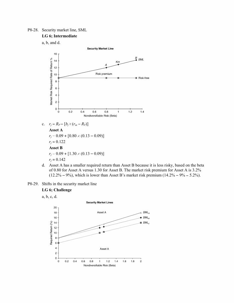
P8-28. Security market line, SML

LG 6; Intermediate

a, b, and d.

c. rj RF [bj (rm RF)]

Asset A

rj 0.09 [0.80 (0.13 0.09)]

rj 0.122

Asset B

rj 0.09 [1.30 (0.13 0.09)]

rj 0.142

d. Asset A has a smaller required return than Asset B because it is less risky, based on the beta

of 0.80 for Asset A versus 1.30 for Asset B. The market risk premium for Asset A is 3.2%

(12.2% 9%), which is lower than Asset B’s market risk premium (14.2% 9% 5.2%).

P8-29. Shifts in the security market line

LG 6; Challenge

a, b, c, d.

b. rj RF [bj (rm RF)]

rA 8% [1.1 (12% 8%)]

rA 8% 4.4%

rA 12.4%

c. rA 6% [1.1 (10% 6%)]

rA 6% 4.4%

rA 10.4%

d. rA 8% [1.1 (13% 8%)]

rA 8% 5.5%

rA 13.5%

e. (1) A decrease in inflationary expectations reduces the required return as shown in the parallel downward shift of the SML.

(2) Increased risk aversion results in a steeper slope, since a higher return would be required

for each level of risk as measured by beta.

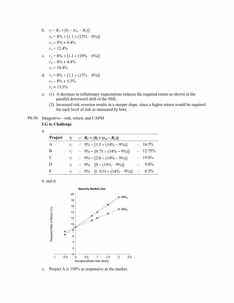
P8-30. Integrative—risk, return, and CAPM

LG 6; Challenge

a.

Project rj RF [bj (rm RF)]

A rj 9% [1.5 (14% 9%)] 16.5%

B rj 9% [0.75 (14% 9%)] 12.75%

C rj 9% [2.0 (14% 9%)] 19.0%

D rj 9% [0 (14% 9%)] 9.0%

E rj 9% [( 0.5) (14% 9%)] 6.5%

b. and d.

c. Project A is 150% as responsive as the market.

Project B is 75% as responsive as the market.

Project C is twice as responsive as the market.

Project D is unaffected by market movement.

Project E is only half as responsive as the market, but moves in the opposite direction as the market.

d. See graph for new SML.

rA 9% [1.5 (12% 9%)] 13.50%

rB 9% [0.75 (12% 9%)] 11.25%

rC 9% [2.0 (12% 9%)] 15.00%

rD 9% [0 (12% 9%)] 9.00%

rE 9% [ 0.5 (12% 9%)] 7.50%

e. The steeper slope of SMLb indicates a higher risk premium than SMLd for these market

conditions. When investor risk aversion declines, investors require lower returns for any

given risk level (beta).

P8-31. Ethics problem

LG 1; Intermediate

Investors expect managers to take risks with their money, so it is clearly not unethical for

managers to make risky investments with other people’s money. However, managers have a duty

to communicate truthfully with investors about the risk that they are taking. Portfolio managers

should not take risks that they do not expect to generate returns sufficient to compensate

investors for the return variability.