ANOVA: Full Factorial Designs - 國立臺灣大學tx.liberal.ntu.edu.tw/~PurpleWoo/Literature/!DataAnalysis/ANOVA... · ANOVA: Full Factorial Designs ... ANOVA tests the null hypothesis

11

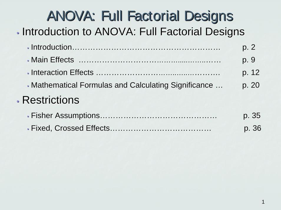
ANOVA: Full Factorial DesignsANOVA: Full Factorial Designs•• Introduction to ANOVA: Full Factorial DesignsIntroduction to ANOVA: Full Factorial Designs

•• IntroductionIntroduction…………………………………………………………………………………………………… p. 2p. 2•• Main Effects Main Effects ……………………………………………………………………..........…………....………… p. 9p. 9•• Interaction Effects Interaction Effects ……………………………………………………....……....…………………….. p. 12p. 12•• Mathematical Formulas and Calculating Significance Mathematical Formulas and Calculating Significance …… p. 20p. 20

•• RestrictionsRestrictions•• Fisher AssumptionsFisher Assumptions……………………………………………………………………………… p. 35p. 35•• Fixed, Crossed EffectsFixed, Crossed Effects…………………………………………………………………… p. 36p. 36

22

Analysis of variance (ANOVA)Analysis of variance (ANOVA) is a statistical technique used to investigate and model the relationship between a response variable and one or more independent variables. Each explanatory variable (factorfactor) consists of two or more categories (levelslevels). ANOVA tests the null hypothesisnull hypothesis that the population means of each level are equal, versus the alternative hypothesisalternative hypothesis that at least one of the level means are not all equal.EXAMPLE 1: A 2003 study was conducted to test if there was a difference in attitudes towards science between boys and girls.

FactorFactor : gender with LevelsLevels : boys and girlsUnitUnit (Experimental Unit or Subject): each individual childResponse VariableResponse Variable: Each child’s score on an attitude assessment.Null HypothesisNull Hypothesis: boys and girls have the same mean score on the assessment.Alternative HypothesisAlternative Hypothesis: boys and girls have different mean scores on the assessment.

Introduction to ANOVAIntroduction to ANOVA

33

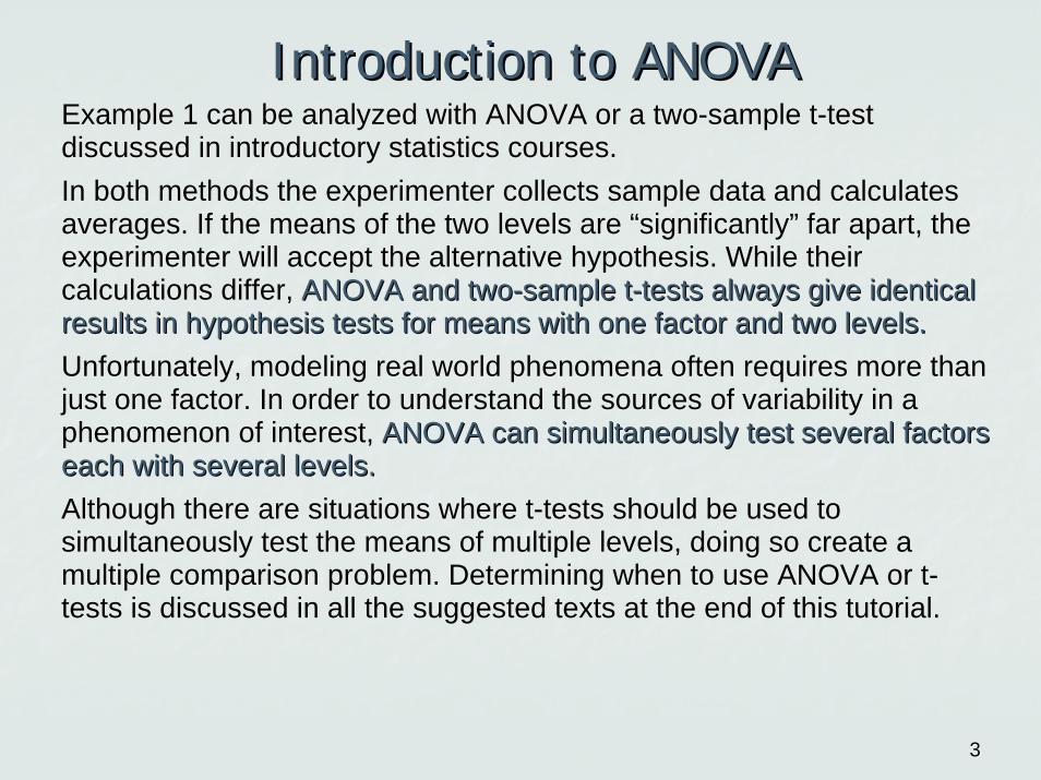
Example 1 can be analyzed with ANOVA or a two-sample t-test discussed in introductory statistics courses.In both methods the experimenter collects sample data and calculates averages. If the means of the two levels are “significantly” far apart, the experimenter will accept the alternative hypothesis. While theircalculations differ, ANOVA and twoANOVA and two--sample tsample t--tests always give identical tests always give identical results in hypothesis tests for means with one factor and two leresults in hypothesis tests for means with one factor and two levels.vels.Unfortunately, modeling real world phenomena often requires more than just one factor. In order to understand the sources of variability in a phenomenon of interest, ANOVA can simultaneously test several factors ANOVA can simultaneously test several factors each with several levels. each with several levels. Although there are situations where t-tests should be used to simultaneously test the means of multiple levels, doing so create a multiple comparison problem. Determining when to use ANOVA or t-tests is discussed in all the suggested texts at the end of this tutorial.

Introduction to ANOVAIntroduction to ANOVA

44

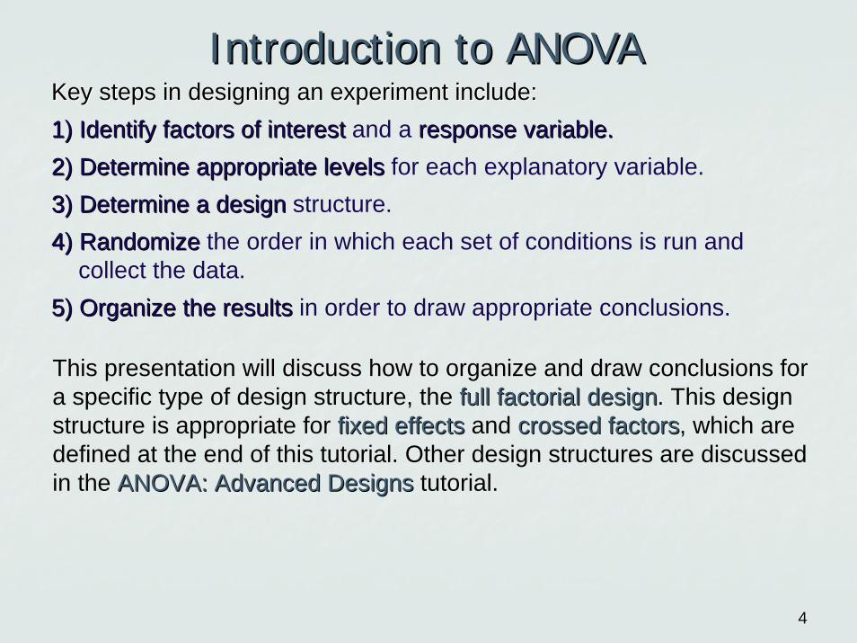
Introduction to ANOVAIntroduction to ANOVAKey steps in designing an experiment include:Key steps in designing an experiment include:1)1) IdentifyIdentify factors of interestfactors of interest and a response variable.response variable.2)2) Determine appropriate levelsDetermine appropriate levels for each explanatory variable. 3) Determine a design 3) Determine a design structure.4)4) RandomizeRandomize the order in which each set of conditions is run and

collect the data.5) Organize the results 5) Organize the results in order to draw appropriate conclusions.

This presentation will discuss how to organize and draw conclusions for a specific type of design structure, the full factorial designfull factorial design. This design structure is appropriate for fixed effectsfixed effects and crossed factorscrossed factors, which are defined at the end of this tutorial. Other design structures are discussed in the ANOVA: Advanced DesignsANOVA: Advanced Designs tutorial.

55

Introduction to Multivariate ANOVAIntroduction to Multivariate ANOVAEXAMPLE 2: Soft Drink Modeling Problem (Montgomery p. 232): A soft drink bottler is interested in obtaining more uniform fill heights in the bottles produced by his manufacturing process. The filling machine theoretically fills each bottle to the correct target height, but in practice, there is variation around this target, and the bottler would like to understand better the sources of this variability and eventually reduce it. The engineer can control three variables during the filling process (each at two levels):

Factor AFactor A: Carbonation with LevelsLevels : 10% and 12%Factor BFactor B: Operating Pressure in the filler with LevelsLevels : 25 and 30 psiFactor CFactor C: Line Speed with LevelsLevels: 200 and 250 bottles produced per minute (bpm)UnitUnit: Each bottleResponse VariableResponse Variable: Deviation from the target fill height Six Hypotheses will be simultaneously tested Six Hypotheses will be simultaneously tested

The steps to designing this experiment include:1)1) IdentifyIdentify factors of interestfactors of interest and a response variable.response variable.2)2) Determine appropriate levelsDetermine appropriate levels for each explanatory variable.

66

Introduction to Multivariate ANOVAIntroduction to Multivariate ANOVA

This is called a 2This is called a 233 full factorial design (i.e. 3 full factorial design (i.e. 3 factors at 2 levels will need 8 runs).factors at 2 levels will need 8 runs). Each row in Each row in this table gives a specific treatment that will be this table gives a specific treatment that will be run. For example, the first row represents arun. For example, the first row represents aspecific test in which thespecific test in which the manufacturing process manufacturing process ran with A set at 10% carbonation, B set atran with A set at 10% carbonation, B set at 25 25 psipsi, and line speed, C, is set at 200 bmp., and line speed, C, is set at 200 bmp.

3) Determine a design structure3) Determine a design structure: Design structures can be very complicated. One of the most basic structures is called the full factorial full factorial designdesign. This design tests every combination of factor levels an equal amount of times. To list each factor combination exactly once

1st Column--alternate every other (20) row2nd Column--alternate every 2 (21) rows3rd Column--alternate every 4th (=22) row

test A B C1234567

10%

8

12%200200200200250250250

10%12%10%12%10%

25012%

2525303025253030

*If there were four factors each at two levels there would be 16 treatments.*If factor C had 3 levels there would be 2*2*3 = 12 treatments.

77

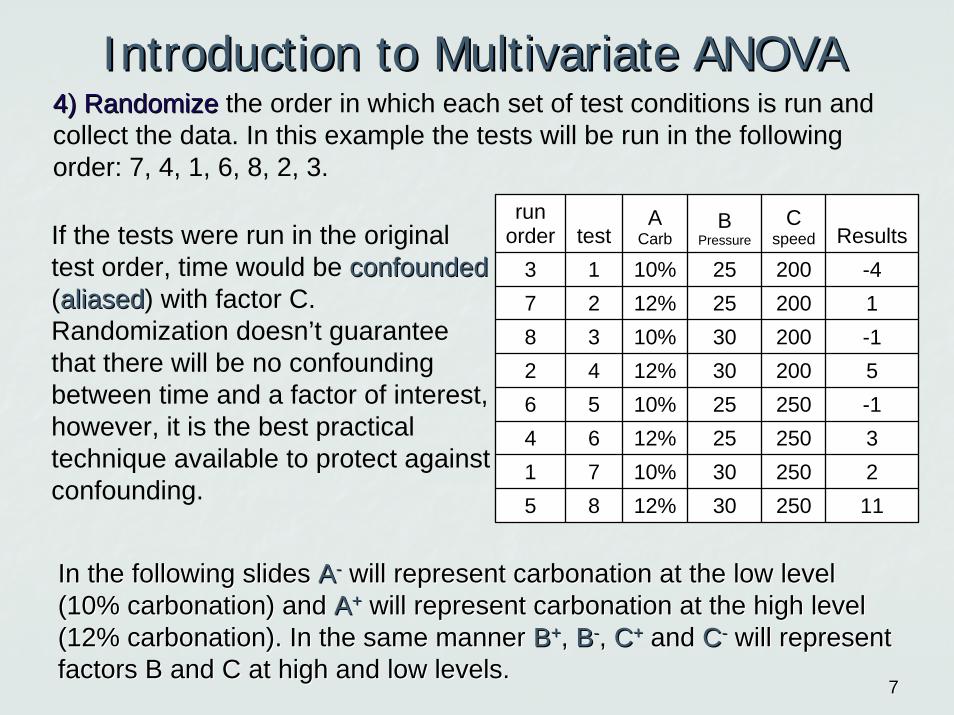
Introduction to Multivariate ANOVAIntroduction to Multivariate ANOVA4)4) RandomizeRandomize the order in which each set of test conditions is run and collect the data. In this example the tests will be run in the following order: 7, 4, 1, 6, 8, 2, 3.

run order test

ACarb

BPressure

Cspeed

3 200200200200250250250250

782641

Results

5

12345678

-41-15-13211

2510%12%10%12%10%12%10%

253030252530

12% 30

If the tests were run in the original test order, time would be confoundedconfounded(aliasedaliased) with factor C. Randomization doesn’t guarantee that there will be no confounding between time and a factor of interest, however, it is the best practical technique available to protect against confounding.

In the following slides In the following slides AA-- will represent carbonation at the low level will represent carbonation at the low level (10% carbonation) and (10% carbonation) and AA++ will represent carbonation at the high level will represent carbonation at the high level (12% carbonation). In the same manner (12% carbonation). In the same manner BB++, , BB--, , CC++ and and CC-- will represent will represent factors B and C at high and low levels.factors B and C at high and low levels.

88

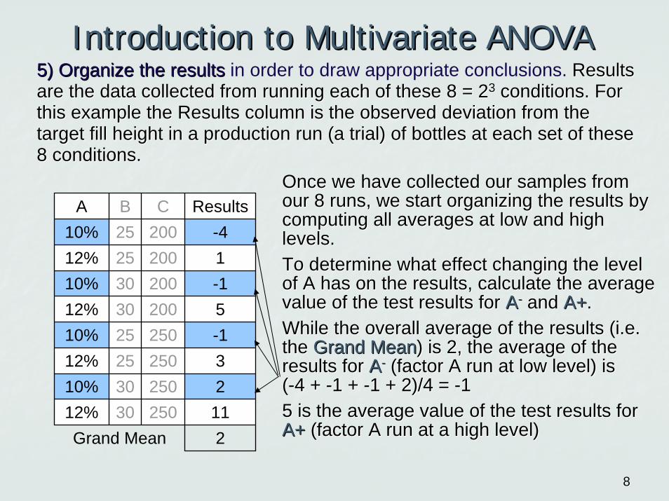
5) Organize the results 5) Organize the results in order to draw appropriate conclusions. Results Results are the data collected from running each of these 8 = 2are the data collected from running each of these 8 = 233 conditions. For conditions. For this example the Results column is the observedthis example the Results column is the observed deviation from the deviation from the target fill height in a production run (a trial) of bottles at etarget fill height in a production run (a trial) of bottles at each set of these ach set of these 8 conditions. 8 conditions.

Once we have collected our samples from Once we have collected our samples from our 8 runs, we start organizing the results by our 8 runs, we start organizing the results by computing all averages at low and high computing all averages at low and high levels. levels. To determine what effect changing the level To determine what effect changing the level of A has on the results, calculate the average of A has on the results, calculate the average value of the test results for value of the test results for AA-- and and A+A+..While the overall average of the results (i.e. While the overall average of the results (i.e. the the Grand MeanGrand Mean) is 2, the average of the ) is 2, the average of the results for results for AA-- (factor A run at low level) is (factor A run at low level) is ((--4 + 4 + --1 + 1 + --1 + 2)/4 = 1 + 2)/4 = --115 is the average value of the test results for 5 is the average value of the test results for A+ A+ (factor A run at a high level)(factor A run at a high level)

A B C Results10% 25 200 -412% 25 200 110% 30 200 -112% 30 200 510% 25 250 -112% 25 250 310% 30 250 212% 30 250 11Grand Mean 2

Introduction to Multivariate ANOVAIntroduction to Multivariate ANOVA

99

A B C Results10% 25 200 -412% 25 200 110% 30 200 -112% 30 200 510% 25 250 -112% 25 250 310% 30 250 212% 30 250 11

Main EffectsMain EffectsThe B and C averages at low and high levels also calculated.

The mean for The mean for BB-- isis ((-- 4 + 1 + 4 + 1 + --1 + 3)/4 = 1 + 3)/4 = --.25.25

The mean for The mean for CC-- isis ((-- 4 +1+4 +1+--1+5)/4 = .251+5)/4 = .25

Notice that each of these eight trial results are used multiple times to calculate six different averages. This can be effectively done because the full factorial design is balancedbalanced. For example when calculating the mean of C low (CC--), there are 2 A highs (AA++) and 2 A lows (AA--), thus the mean of A is not confounded with the mean of C. This balance is true for all mean calculations.

A Avg. B Avg. C Avg.

low -1 -.25 .25high 5 4.25 3.75

1010

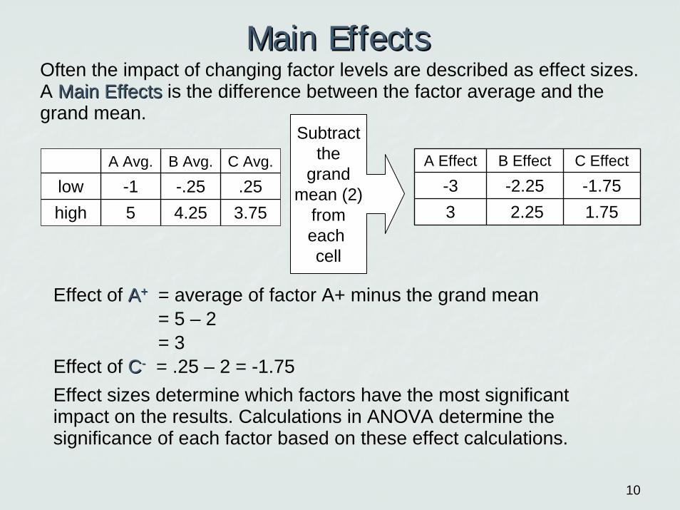
Main EffectsMain EffectsOften the impact of changing factor levels are described as effect sizes. A Main EffectsMain Effects is the difference between the factor average and the grand mean.

A Effect B Effect C Effect

-3 -2.252.253

-1.751.75

Subtract the

grand mean (2)

from each cell

Effect of AA++ = = average of factor A+ minus the grand mean= 5 – 2= 3

Effect of CC-- = .= .25 – 2 = -1.75Effect sizes determine which factors have the most significant impact on the results. Calculations in ANOVA determine the significance of each factor based on these effect calculations.

A Avg. B Avg. C Avg.

low -1 -.25 .25high 5 4.25 3.75

1111

Main EffectsMain EffectsMain Effects PlotsMain Effects Plots are a quick and efficient way to visualize effect size. are a quick and efficient way to visualize effect size. The grand mean, 2, is plotted as a horizontal line. The average The grand mean, 2, is plotted as a horizontal line. The average result is result is represented by dots for each factor level.represented by dots for each factor level.The Y axis is always the same for each factor in Main Effects PlThe Y axis is always the same for each factor in Main Effects Plots. ots. Factors with steeper slopes have larger effects and thus larger Factors with steeper slopes have larger effects and thus larger impacts impacts on the results. on the results.

Mea

n o

f R

esu

lts

12%10%

5

4

3

2

1

0

-1

30psi25psi 250200

Carbonation Pressure Speed

Main Effects Plot for Results (Bottle Fill Heights)

A Avg.

B Avg.

C Avg.

low -1 -.25 .25high 5 4.25 3.75

This graph shows that This graph shows that AA+ +

has a higher mean fill has a higher mean fill height than height than AA--. . BB++ and and CC+ +

also have higher means also have higher means than than BB-- and and CC--

respectively. In addition, respectively. In addition, the effect size of factor A, the effect size of factor A, Carbonation, is larger than Carbonation, is larger than the other factor effects.the other factor effects.

1212

A B C Results

10% 25 200 -412% 25 200 110% 30 200 -112% 30 200 510% 25 250 -112% 25 250 310% 30 250 212% 30 250 11

Interaction EffectsInteraction Effects

AB Avg.

AA--BB--

AA++BB--

AA--BB++

AA++BB++

-2.52.00.58.0

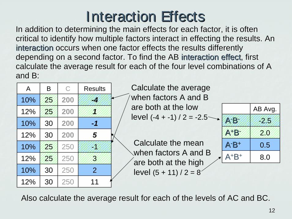
In addition to determining the main effects for each factor, it In addition to determining the main effects for each factor, it is often is often critical to identify how multiple factors interact in effecting critical to identify how multiple factors interact in effecting the results. An the results. An interactioninteraction occurs whenoccurs when one factor effects the results differently factor effects the results differently depending on a second factor. To find the AB depending on a second factor. To find the AB interaction effectinteraction effect, first , first calculate the average result for each of the four level combinatcalculate the average result for each of the four level combinations of A ions of A and B: and B:

Calculate the average when factors A and B are both at the low level (-4 + -1) / 2 = -2.5

Calculate the mean when factors A and B are both at the high level (5 + 11) / 2 = 8

Also calculate the average result for each of the levels of AC aAlso calculate the average result for each of the levels of AC and BC.nd BC.

1313

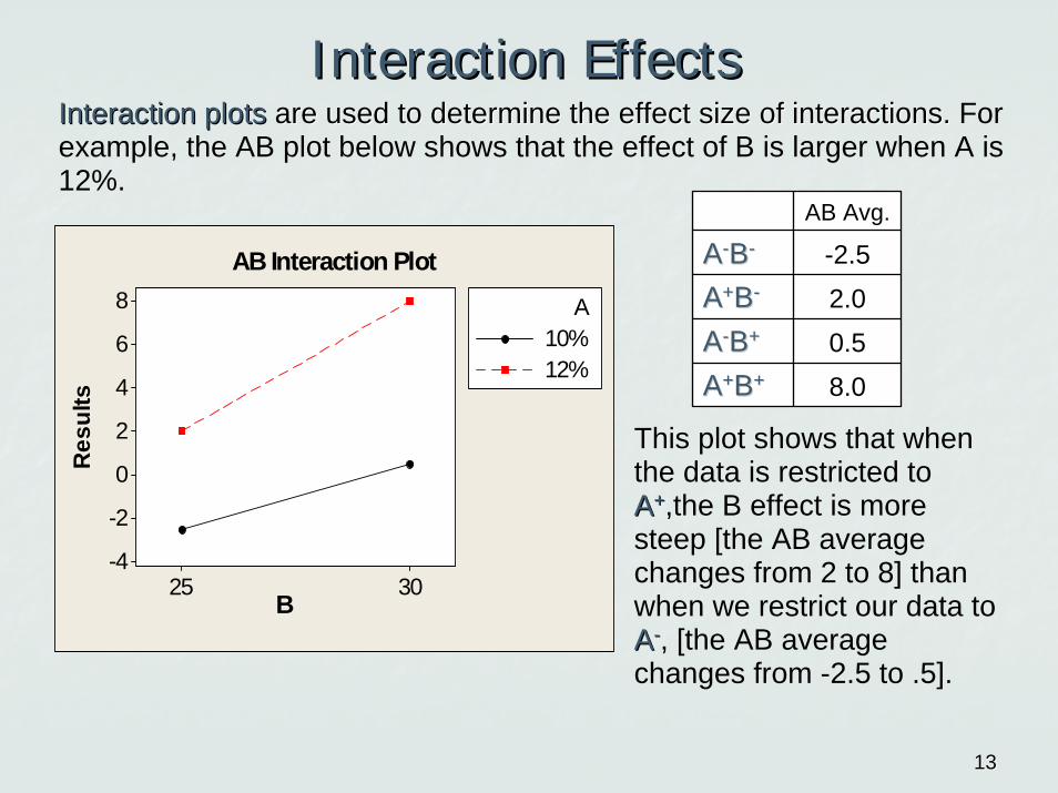
Interaction EffectsInteraction EffectsInteraction plotsInteraction plots are used to determine the effect size of interactions.are used to determine the effect size of interactions. For example, the AB plot below shows that the effect of B is larger when A is 12%.

B

Res

ults

3025

8

6

4

2

0

-2

-4

A10%12%

AB Interaction Plot

AB Avg.

AA--BB--

AA++BB--

AA--BB++

AA++BB++

-2.52.00.58.0

This plot shows that when the data is restricted to AA++,the B effect is more steep [the AB average changes from 2 to 8] than when we restrict our data to AA--, [the AB average changes from -2.5 to .5].

1414

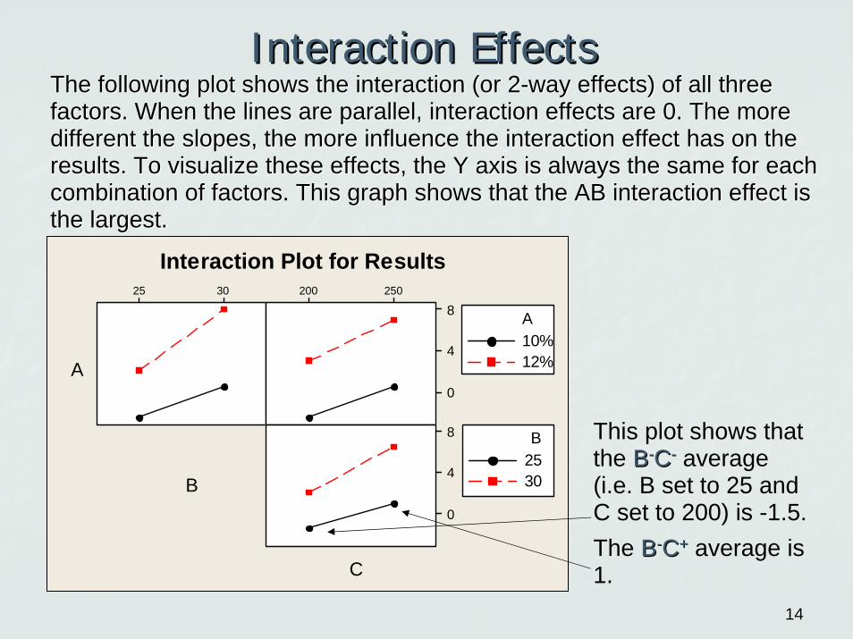
Interaction EffectsInteraction EffectsThe following plot shows the interaction (or 2The following plot shows the interaction (or 2--way effects) of all three way effects) of all three factors. When the lines are parallel,factors. When the lines are parallel, interaction effects are 0. The more interaction effects are 0. The more different the slopes, the more influence the interaction effect different the slopes, the more influence the interaction effect has on the has on the results. To visualize these effects, the Y axis is always the saresults. To visualize these effects, the Y axis is always the same for each me for each combination of factorscombination of factors. This graph shows that the AB interaction effect is This graph shows that the AB interaction effect is the largest.the largest.

3025 250200

8

4

0

8

4

0

A10%12%

B2530

Interaction Plot for Results

A

B

C

This plot shows that the BB--CC-- average (i.e. B set to 25 and C set to 200) is -1.5.The BB--CC++ average is 1.

1515

A B C ResultsAB

Avg. A

EffectGrand Avg.

-2.5 22222222

2.00.58.0-2.52.00.5

-4

8.0

-33-33-33-33

1-15-13211

B Effect

10% 25 200 -2.25-2.252.252.25-2.25-2.252.252.25

12% 25 20010% 30 20012% 30 20010% 25 25012% 25 25010% 30 25012% 30 250

Interaction EffectsInteraction EffectsTo calculate the size of each twoTo calculate the size of each two--way way interaction effect, calculate the effect, calculate the average of every level of each factor combination as well as allaverage of every level of each factor combination as well as all other other effects that impact those averages.effects that impact those averages.The A effect, B effect, and overall effect (grand mean) influencThe A effect, B effect, and overall effect (grand mean) influence the e the AB AB interaction effect. Factor C is completely ignored in these calcinteraction effect. Factor C is completely ignored in these calculations.ulations. Note that these values are placed in rows corresponding to the original dathese values are placed in rows corresponding to the original dataset. aset.

These two rows show These two rows show the AB average, the A the AB average, the A effect, the B effect, effect, the B effect, and the grand mean and the grand mean when when AA-- and and BB--..

These two rows show These two rows show thethe AB average, the A AB average, the A effect, the B effect, effect, the B effect, and the grand mean and the grand mean when when AA-- and and BB++.

1616

A B C ResultsAB

Avg. A

EffectGrand Avg.

-2.5 2222222

2

2.00.58.0-2.52.00.5

-4

8.0

-33-33-33-3

3

1-15-132

11

AB Effect

0.75-0.75-0.750.750.75-0.75-0.75

0.75

B Effect

10% 25 200 -2.25-2.252.252.25-2.25-2.252.25

2.25

12% 25 20010% 30 20012% 30 20010% 25 25012% 25 25010% 30 250

12% 30 250

Interaction EffectsInteraction EffectsEffect sizeEffect size is the difference between the average and the partial fit.is the difference between the average and the partial fit.Partial fitPartial fit = the effect of all the influencing factors. = the effect of all the influencing factors. For main effects, the partial fit is the grand mean.For main effects, the partial fit is the grand mean.

Effect of AB = Effect of AB = ABAB Avg.Avg.–– [effect of A + effect of B + the grand mean][effect of A + effect of B + the grand mean]Effect for Effect for AA--BB-- = = --2.5 2.5 –– [[--3 + 3 + --2.25 +2] = .752.25 +2] = .75Effect for Effect for AA--BB++ = 0.5 = 0.5 –– [ [ --3 + 2.25 +2] = 3 + 2.25 +2] = --.75.75

subtract the

partialfit

from eachlevel

average

1717

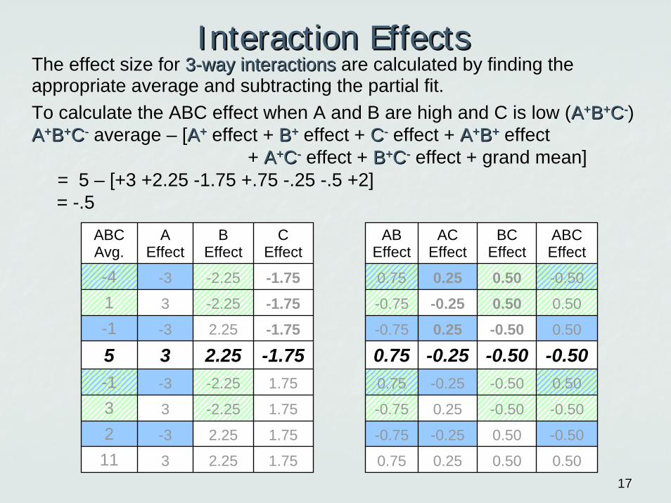
Interaction EffectsInteraction EffectsThe effect size for 33--way interactionsway interactions are calculated by finding the appropriate average and subtracting the partial fit. To calculate the ABC effect when A and B are high and C is low (AA++BB++CC--) AA++BB++CC-- average – [AA++ effect + BB++ effect + CC-- effect + AA++BB++ effect

+ AA++CC-- effect + BB++CC-- effect + grand mean]= 5 – [+3 +2.25 -1.75 +.75 -.25 -.5 +2]= -.5

ABC Avg.

A Effect

B Effect

C Effect

AB Effect

AC Effect

BC Effect

ABC Effect

-41-15-13211

-0.50

0.50

0.50

-0.500.50

-0.50

-0.50

0.75

0.50

-0.75

0.500.25-0.250.25

-0.25-0.25

0.25

-0.75

-0.25

0.50-0.50

-0.50-0.50

-0.50

0.25

0.750.75

0.50

0.50

-0.75

-0.75

0.75

-3 -2.25 -1.753 -2.25 -1.75-3 2.25 -1.75

3 2.25 -1.75-3 -2.25 1.75

3 -2.25 1.75

-3 2.25 1.75

3 2.25 1.75

1818

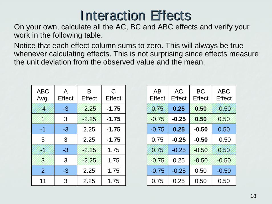
Interaction EffectsInteraction EffectsOn your own, calculate all the AC, BC and ABC effects and verify your work in the following table. Notice that each effect column sums to zero. This will always be true whenever calculating effects. This is not surprising since effects measure the unit deviation from the observed value and the mean.

ABC Avg.

A Effect

B Effect

C Effect

AB Effect

AC Effect

BC Effect

ABC Effect

-4

1

-1

5

-1

3

2

11

-0.50

0.50

0.50

-0.50

0.50

-0.50

-0.50

0.75

0.50

-0.75

0.500.25-0.250.25-0.25-0.25

0.25

-0.75

-0.25

0.50-0.50-0.50-0.50

-0.50

0.25

0.75

0.75

0.50

0.50

-0.75

-0.75

0.75

-3 -2.25 -1.753 -2.25 -1.75-3 2.25 -1.753 2.25 -1.75-3 -2.25 1.75

3 -2.25 1.75

-3 2.25 1.75

3 2.25 1.75

1919

Interaction EffectsInteraction Effects

A B C ResultsAB

Avg. AC

Avg.BC

Avg.ABC Avg.- 41-15--1133

22

1111

10%12%10%12%10%12%10%

-2.5

12%

ABC Effect

-1.5-2.5 -0.500.500.50-0.500.50-0.50-0.500.50

2.00.5

-1.53.0-2.53.08.0

0.50.57.07.0

2.02.01.01.01.01.0

6.56.5

-2.52.0

0.50.5

7.07.0 6.56.50.58.0

25 200 - 425 200 130 200 -130 200 525 250 -125 250 330 250 230 250 11

Also note that the ABC Average column is identical to the results column. In this example, there are 8 runs (observations) and 8 ABC interaction levels. There are not enough runs to distinguish the ABC interaction effect from the basic sample to sample variability. In factorial designs, each run needs to be repeated more than once for the highest-order interaction effect to be measured. However, this is not necessarily a problem because it is often reasonable to assume higher-order interactions are not significant.

2020

Mathematical CalculationsMathematical CalculationsEffect plots help visualize the impact of each factor combination and identify which factors are most influential. However, a statistical hypotheses test is needed in order to determine if any of these effects are significantsignificant. Analysis of variance (ANOVAANOVA) consists of simultaneous hypothesis tests to determine if any of the effects are significant. Note that saying “factor effects are zero” is equivalent to saying “the means for all levels of a factor are equal”. Thus, for each factor combination ANOVA tests the null hypothesis that the population means of each level are equal, versus them not all being equal. Several calculations will be made for each main factor and interaction interaction termterm:

Sum of Squares (SS)Sum of Squares (SS) = sum of all the squared effects for each factorDegrees of Freedom (Degrees of Freedom (dfdf)) = number of free units of information Mean Square (MS)Mean Square (MS) = SS/df for each factorMean Square Error (MSE)Mean Square Error (MSE) = pooled variance of samples within each level

FF--statistic statistic = MS for each factor/MSE

2121

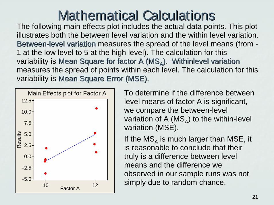
Mathematical CalculationsMathematical CalculationsThe following main effects plot includes the actual data points. This plot illustrates both the between level variation and the within level variation. BetweenBetween--level variationlevel variation measures the spread of the level means (from -1 at the low level to 5 at the high level). The calculation for this variability is Mean Square for factor A (MSMean Square for factor A (MSAA). ). WithinlevelWithinlevel variationvariationmeasures the spread of points within each level. The calculation for this variability is Mean Square Error (MSE).Mean Square Error (MSE).

p-value = 0.105

To determine if the difference between level means of factor A is significant, we compare the between-level variation of A (MSA) to the within-level variation (MSE). If the MSA is much larger than MSE, it is reasonable to conclude that their truly is a difference between level means and the difference we observed in our sample runs was not simply due to random chance.

Factor A

Res

ults

1210

12.5

10.0

7.5

5.0

2.5

0.0

-2.5

-5.0

Main Effects plot for Factor A

2222

Mathematical CalculationsMathematical CalculationsThe first dotplot of the Results vs. factor A shows that the between level variation of A (from -1 to 5) is not significantly larger than the within level variation (the variation within the 4 points in AA-- and the 4 points in AA++).

1-1

12.5

10.0

7.5

5.0

2.5

0.0

-2.5

-5.01-1

Results Results(2)

Dotplot of Results, Results(2) vs A The second dotplot of Results(2) vs. factor A uses a hypothetical data set. The between-level variation is the same in both Results and Results(2). However the within-level variation is much larger for Results than Results(2). With Results(2) we are much more confident hat the effect of Factor A is not simply due to random chance.

Even though the averages are the same (and thus the MSA are identical) in both data sets, Results(2) provides much stronger evidence that we can reject the null hypothesis and conclude that the effect of AA-- is different than the effect of AA+ + .

AA-- AA-- AA++AA++

2323

Mathematical CalculationsMathematical Calculations

A Effect B Effect C Effect

-3 -2.25-2.252.252.25-2.25-2.252.25

3 2.25 1.75

3--1.751.75--1.751.75--1.751.75--1.751.751.751.75

-33-33-3 1.75

0 0 0

A EffectSquared

B EffectSquared

C EffectSquared

9 5.06255.06255.06255.06255.06255.06255.0625

9 5.0625 3.0625

93.06253.06253.06253.06253.06253.0625

99999 3.0625

SS 72.0 40.5 24.5

Sum of Squares (SS)Sum of Squares (SS) is calculated by summing the squared factor effect for each run. The table below shows the calculations for the SS for factor A (written SSA) = 72.0 = 4(-3)2 + 4(3)2

The table below also shows SSB = 40.5 and SSC = 24.5

Sum

2424

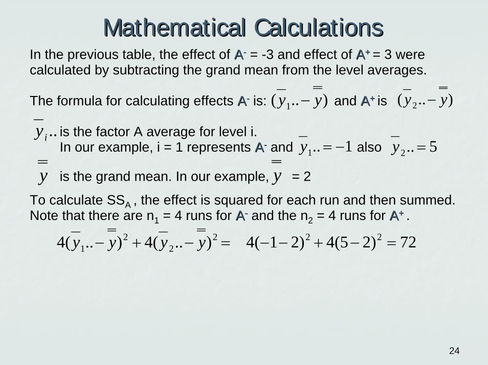
Mathematical CalculationsMathematical CalculationsIn the previous table, the effect of AA-- = -3 and effect of AA+ + = 3 were calculated by subtracting the grand mean from the level averages.

The formula for calculating effects AA-- is: and AA+ + is

is the factor A average for level i. In our example, i = 1 represents AA-- and also

is the grand mean. In our example, = 2

To calculate SSA , the effect is squared for each run and then summed. Note that there are n1 = 4 runs for AA-- and the n2 = 4 runs for AA+ + .

..iy

y

)..( 1 yy − )..( 2 yy −

1..1 −=y 5..2 =y

y

72)25(4)21(4)..(4)..(4 2222

21 =−+−−=−+− yyyy

2525

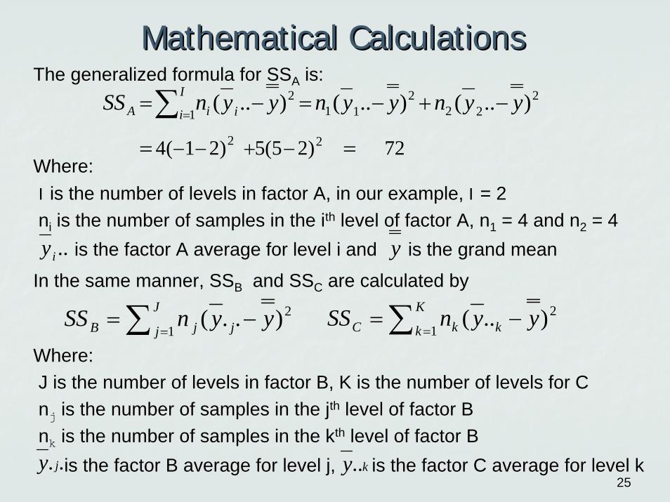
Mathematical CalculationsMathematical CalculationsThe generalized formula for SSA is:

Where:I is the number of levels in factor A, in our example, I = 2ni is the number of samples in the ith level of factor A, n1 = 4 and n2 = 4

is the factor A average for level i and is the grand mean

In the same manner, SSB and SSC are calculated by

Where:J is the number of levels in factor B, K is the number of levels for Cnj is the number of samples in the jth level of factor B nk is the number of samples in the kth level of factor B

is the factor B average for level j, is the factor C average for level k

..iy y

∑ =−=

J

j jjB yynSS1

2)..( ∑ =−=

K

k kkC yynSS1

2)..(

.. jy ky..

72)25(5)21(4 22

222

2111

2 )..()..()..(

==

−+−=−=

−+−−

∑ =yynyynyynSS I

i iiA

2626

is the mean of all AB factor runs at the i, j level.On your own, calculate the SSACand SSBC

Mathematical CalculationsMathematical Calculations

SS 4.5 0.5 2

Sum of Squares (SS)Sum of Squares (SS) for interactions is also calculated by summing the squared factor effect for each run. The table below shows the calculations for SSAB = 4.5 = 2(.75)2 + 2(-.75)2 + 2(-.75)2 + 2(.75)2

AB EffectSquared

AC EffectSquared

BC EffectSquared

.5625.5625

.5625.5625

.5625.5625

.5625.5625

.5625.5625

.5625.5625

.5625.5625

.5625.5625

.25.25.0625.0625.0625.0625.0625.0625.0625.0625.0625.0625.0625.0625

.0625.0625

.25.25

.25.25

.25.25

.25.25

.25.25

.25.25.0625.0625 .25.25

AB Effect

AC Effect

BC Effect

0.75-0.75-0.750.750.75-0.75-0.750.75

0.500.25-0.250.25-0.25-0.250.25-0.25

0.50-0.50-0.50-0.50-0.500.50

0.25 0.50

( )∑∑ ∑∑∑

=

= ===

=−−−+−−−=

−−−==

J

j jjjjjj

I

i

I

i jijiijJ

jth

ijJ

jAB

yyyynyyyyn

yyyyneffectlevelijnSS

12

2222

111

1 12

12

1

5.4).....().....(

).....()(

nij is the number of samples in level ij. In our example each ij level has 2 samples.

.ijy

2727

Mathematical CalculationsMathematical Calculations

A Effect B Effect C Effect

-3 -2.25-2.252.252.25-2.25-2.252.25

3 2.25 1.75

3--1.751.75--1.751.75--1.751.75--1.751.751.751.75

-33-33-3 1.75

Degrees of Freedom (Degrees of Freedom (dfdf)) = number of free units of information. In the example provided, there are 2 levels of factor A. Since we require that the effects sum to 0, knowing AA-- automatically forces a known AA+ + . If there are I levels for factor A, one level is fixed if we know the other I-1 levels. Thus, when there are I levels for a main factor of interest, there is I-1 free pieces of information.

For a full factorial ANOVA, df for a main effect are the number of levels minus one:

dfA = I - 1

dfB = J - 1

dfC = K - 1

2828

Mathematical CalculationsMathematical Calculations

A Effect

B Effect

AB Effect

-3 -2.25-2.252.252.25-2.25-2.252.25

3 2.25 0.75

30.75-0.75-0.750.750.75-0.75

-33-33-3 -0.75

For the AB interaction term there are I*J effects that are calculated. Each effect is a piece of information. Restrictions in ANOVA require:

Thus, general rules for a factorial ANOVA:dfAB = IJ – [(I-1) + (J-1) + 1] = (I-1)(J-1) dfBC = (J-1)(K-1)

dfAC = (I-1)(K-1) dfABC = (I-1)(J-1)(K-1)

Note the relationship between the calculation of dfAB and the calculation of the AB interaction effect.

dfAB = # of effects – [pieces of information already accounted for]

= # of effects – [dfA + dfB + 1]

1)AB factor effects sum to 0. This requires 1 piece of information to be fixed.

2)The AB effects within AA-- sum to 0. In our example, the AB effects restricted to AA-- are (.75, -.75,.75,-.75). The same is true for the AB effect restricted to AA+ + . This requires 1 piece of information to be fixed in each level of A. Since 1 value is already fixed in restriction1), this requires I-1 pieces of information.

3) The AB effects within each level of B. This requires J-1 pieces of information.

2929

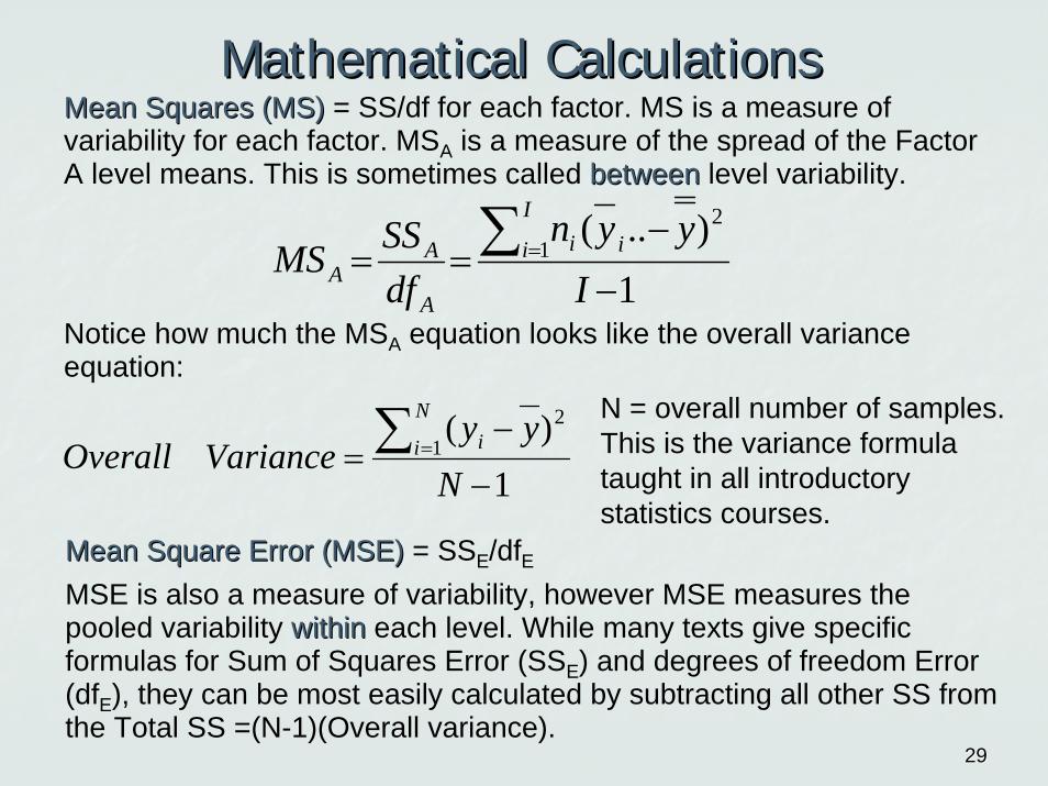
Mathematical CalculationsMathematical CalculationsMean Squares (MS)Mean Squares (MS) = SS/df for each factor. MS is a measure of variability for each factor. MSA is a measure of the spread of the Factor A level means. This is sometimes called betweenbetween level variability.

Notice how much the MSA equation looks like the overall variance equation:

1)..(

12

−

−== ∑ =

Iyyn

dfSSMS

I

i ii

A

AA

Mean Square Error (MSE)Mean Square Error (MSE) = SSE/dfEMSE is also a measure of variability, however MSE measures the pooled variability withinwithin each level. While many texts give specific formulas for Sum of Squares Error (SSE) and degrees of freedom Error (dfE), they can be most easily calculated by subtracting all other SS from the Total SS =(N-1)(Overall variance).

1)(

12

−

−= ∑ =

Nyy

VarianceOverallN

i iN = overall number of samples. This is the variance formula taught in all introductory statistics courses.

3030

Mathematical CalculationsMathematical CalculationsFF--statistic statistic = MS for each factor/MSE. The F-statistic is a ratio of the between variability over the within variability. If the true population mean of AA-- equals true population mean of AA++, then we would expect the variation between levels in our sample runs to be equivalent to the variation within levels. Thus we would expect the F-statistic would be close to 1.If the F-statistic is large, it seems unlikely that the population means of each level of factor A are truly equal.Mathematical theory proves that if the appropriate assumptions hold, the F-statistic follows an F distribution with dfA (if testing factor A) and dfEdegrees of freedom. The pp--valuevalue is looked up in an F table and gives the likelihood of observing an F statistic at least this extreme (at least this large) assuming that the true population factor has equal level means. Thus, when the p-value is small (i.e. less than 0.05 or 0.1) the effect size of that factor is statistically significant.

3131

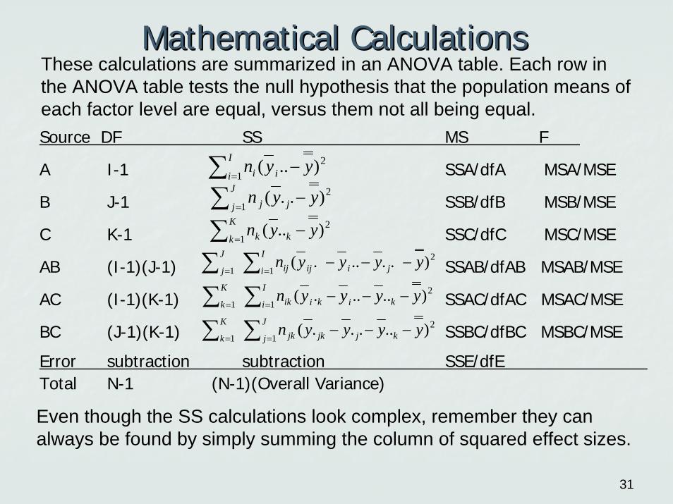
Mathematical CalculationsMathematical CalculationsThese calculations are summarized in an ANOVA table. Each row inthe ANOVA table tests the null hypothesis that the population means of each factor level are equal, versus them not all being equal. Source DF SS MS F

A I-1 SSA/dfA MSA/MSE

B J-1 SSB/dfB MSB/MSE

C K-1 SSC/dfC MSC/MSE

AB (I-1)(J-1) SSAB/dfAB MSAB/MSE

AC (I-1)(K-1) SSAC/dfAC MSAC/MSE

BC (J-1)(K-1) SSBC/dfBC MSBC/MSE

Error subtraction subtraction SSE/dfETotal N-1 (N-1)(Overall Variance)

∑ =−

I

i ii yyn1

2)..(

∑ =−

J

j jj yyn1

2)..(

∑ =−

K

k kk yyn1

2)..(

∑∑ ==−−−

I

i jiijijJ

jyyyyn

12

1).....(

∑∑ ==−−−

I

i kikiikK

kyyyyn

12

1).....(

∑∑ ==−−−

J

j kjjkjkK

kyyyyn

12

1).....(

Even though the SS calculations look complex, remember they can always be found by simply summing the column of squared effect sizes.

3232

Mathematical CalculationsMathematical CalculationsFor the bottle filling example, we calculate the following results.Source DF SS MS F p-valueA 1 72.0 72.0 36.00 0.105B 1 40.5 40.5 20.25 0.139C 1 24.5 24.5 12.25 0.177A*B 1 4.5 4.5 2.25 0.374A*C 1 0.5 0.5 0.25 0.705B*C 1 2.0 2.0 1.00 0.500Error 1 2.0 2.0Total 7 146.0

Each row in the ANOVA table represents a null hypothesis that the means of each factor level are equal. Each row shows an F statistic and a p-value corresponding to each hypothesis. When the p-value is small (i.e. less than 0.05 or 0.1) reject the null hypothesis and conclude that the levels of the corresponding factor are significantly different (i.e. conclude that the effect sizes of that factor are significantly large).

3333

Mathematical CalculationsMathematical CalculationsViewing the effect plots with the appropriate p-values clearly shows that while factor A (Carbonation) had the largest effect sizes in our sample of 8 runs, effect sizes this large would occur in 10.5% of our samples even if factor A truly has no effect on the Results.Effect sizes as large as were observed for factor C (Speed) would occur in 17.7% of samples of 8 runs even if there truly was no difference between the mean Results of speed run at 200 bpm and at 250 bpm.

Res

ults

1210

12.5

10.0

7.5

5.0

2.5

0.0

-2.5

-5.03025 250200

Carbonation Pressure SpeedMain Effects Plot

p-value = 0.139 p-value = 0.177p-value = 0.105

3434

Mathematical CalculationsMathematical Calculations

Factor C: Speed

Res

ults

250200

12.5

10.0

7.5

5.0

2.5

0.0

-2.5

-5.0

p-value = 0.5

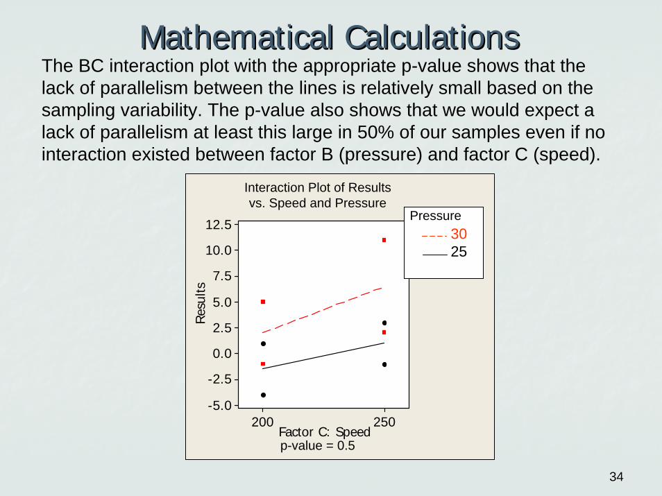
Interaction Plot of Resultsvs. Speed and Pressure

3025

Pressure

The BC interaction plot with the appropriate p-value shows that the lack of parallelism between the lines is relatively small based on the sampling variability. The p-value also shows that we would expect a lack of parallelism at least this large in 50% of our samples even if no interaction existed between factor B (pressure) and factor C (speed).

3535

Fisher AssumptionsFisher AssumptionsIn order for the p-values to be accurate, the F statistics that are calculated in ANOVA are expected to follow the F distribution. While we will not discuss the derivation of the F distribution, it is valuable to understand the six Fisher assumptions that are used in the derivation. If any experimental data does not follow these assumptions, then ANOVA give incorrect p-values.1) The unknown true population means (and effect sizes) of every treatment are constant.2) The additivity assumption: each observed sample consists of a true population mean for a particular level combination plusplus sampling error.3) Sampling errors are normally distributed and 4) Sampling errors are independent. Several residual plots should be made to validate these assumptions every time ANOVA is used.5) Every level combination has equivalent variability among its samples. ANOVA may not be reliable if the standard deviation within any level is more than twice as large as the standard deviation of any other level. 6) Sampling errors have a mean of 0, thus the average of the samples within a particular level should be close to the true level mean.

3636

Advanced Designs:Advanced Designs:Fixed Vs. Random EffectsFixed Vs. Random Effects

Fixed factors: the levels tested represent all levels of interestRandom factors: the levels tested represent a random sample of an entire set of possible levels of interest.EXAMPLE 3: A statistics class wanted to test if the speed at which a game is played (factor A: slow, medium, or fast speed) effects memory. They created an on-line game and measured results which were the number of sequences that could be remembered. If four friends wanted to test who had the best memory. They each play all 3 speed levels in random orders. A total of 12 games were played. Since each student effect represents a specific level that is of interest, student should be considered a fixed effect.If four students were randomly selected from the class and each student played each of the three speed levels. A total of 12 games were played. How one student compared to another is of no real interest. The effect of any particular student has no meaning, but the student-to-student variability should be modeled in the ANOVA. Student should be considered a random effect.

3737

Advanced DesignsAdvanced DesignsCrossed Vs. Nested EffectsCrossed Vs. Nested Effects

Factors A and B are crossed if every level of A can occur in every level of B. Factor B is nested in factor A if levels of B only have meaning within specific levels of A.EXAMPLE 3 (continued): If 12 students from the class were assigned to one of the three speed levels (4 within each speed level), students would be considered nested within speed. The effect of any student has no meaning unless you also consider which speed they were assigned. There are 12 games played and MSE would measure student to student variability. Since students were randomly assigned to specific speeds, the student speed interaction has no meaning in this experiment.If four friends wanted to test who had the best memory they could each play all 3 speed levels. There would be a total of 12 games played. Speed would be factor A in the ANOVA with 2 df. Students would be factor B with 3 df. Since the student effect and the speed effect are both of interest these factors would be crossed. In addition the AB interaction would be of interest.