ANOVA exercise class Sylvain 03/11/2014 Organization • Corrected series that are not picked up can be found in a tray in J68 • I’m always available for questions by email or during the exercise class • Please complain if anything is unclear about the solution of a series, my corrections, or during the exercise class Comments about series 2 A few confusions about contrasts: • ∑ i λ i = 0 is necessary for a contrast • Two contrasts C 1 and C 2 are orthogonal iff ∑ i λ 1 i λ 2 i =0 • Geometrically: ∑ i λ 1 i λ 2 i = scalar product = 0 <=> perpendicular • Example: (1, 0, -1) and (1, -2, 1) are orthogonal • Example: (1, 0, -1) and (1, -2, 2) are not orthogonal How to test if a set of contrasts are all orthogonal? • Solution 1: Test all pairs of contrasts one by one • Solution in R: write the contrast in a matrix C, with each column being a contrast and check that C C is diagonal. • Why does it work? How to test if a set of contrasts are all orthogonal? (2) • Let’s look at the element ij of C C: •(C C) ij = C ·i C ·j , which is. . . • . . . the scalar product of contrast i with contrast j , which is. . . • ... ∑ k λ i k λ j k , which. . . • . . . equals 0 iff they are orthogonal! • So if all off-diagonal elements of C t C are 0, it means that all pairs of contrasts are orthogonal. 1

Welcome message from author
This document is posted to help you gain knowledge. Please leave a comment to let me know what you think about it! Share it to your friends and learn new things together.
Transcript
ANOVA exercise classSylvain
03/11/2014
Organization
• Corrected series that are not picked up can be found in a tray in J68
• I’m always available for questions by email or during the exercise class
• Please complain if anything is unclear about the solution of a series, my corrections, or during theexercise class
Comments about series 2
A few confusions about contrasts:
•∑
i λi = 0 is necessary for a contrast
• Two contrasts C1 and C ′2 are orthogonal iff∑
i λ1iλ
2i = 0
• Geometrically:∑
i λ1iλ
2i = scalar product = 0 <=> perpendicular
• Example: (1, 0,−1) and (1,−2, 1) are orthogonal
• Example: (1, 0,−1) and (1,−2, 2) are not orthogonal
How to test if a set of contrasts are all orthogonal?
• Solution 1: Test all pairs of contrasts one by one
• Solution in R: write the contrast in a matrix C, with each column being a contrast and check that C ′Cis diagonal.
• Why does it work?
How to test if a set of contrasts are all orthogonal? (2)
• Let’s look at the element ij of C ′C:
• (C ′C)ij = C ′·iC·j , which is. . .
• . . . the scalar product of contrast i with contrast j, which is. . .
• . . .∑
k λikλ
jk, which. . .
• . . . equals 0 iff they are orthogonal!
• So if all off-diagonal elements of CtC are 0, it means that all pairs of contrasts are orthogonal.
1
One-way ANOVA with R
• Now you should be expert of one-way ANOVA, are you?
• R formula: aov(Y~Treatment + Block, data=dat)
• Don’t write: aov(dat$Y ~ dat$Treatment + dat$Block)
• Or worse: aov(dat$Y ~ as.numeric(dat$Treatment) + as.numeric(dat$Block))
One-way ANOVA with R (2)
• Many people forgot to include the blocking variable! don’t.
• Transform the factor variables with as.factor().
• In exercise 4, many people treated land as numeric, which messes up all the results and interpretation.
End of comments about series 2
• Questions about series 2?
• Questions about contrasts?
• Questions about one-way ANOVA, blocking, etc?
Review
• Two-way ANOVA
• Additive model
• Model with interaction
• Three-way ANOVA
Two-way ANOVA
We are now interested in the joint effect of two variables on an outcome Y.
Additive model:
Yij = µ+Ai +Bj + εij
Two-way ANOVA: an example (1)
Disclaimer: the data used in this example is completely fake.
• Age category: under 30 (0), over 30 (1)
• Education: Higher education(1), or not (0)
• Y: Income (in k CHF)
2
In R:
set.seed(3)Age <- as.factor( rep( c( 0,0, 1,1), 2) )levels(Age) <- c('young', 'old')Ed <- as.factor( rep( c( 0,1, 0,1), 2) )levels(Ed) <- c('not higher', 'higher')y <- c(4, 3, 5, 10, 3.5, 3, 4, 9.5)# y <- rep( c( 4, 3, 5, 10), 2) + rnorm(8, 0, 1)dat <- data.frame(y, Age, Ed)
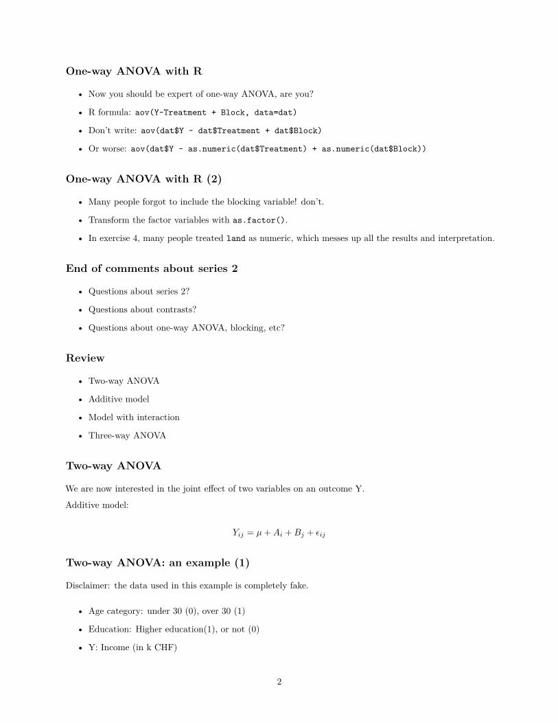
Two-way ANOVA: an example (2)
Ok, there seem to be something going on. . .
par(mfrow=c(1,2))plot(y ~ Age, data=dat)plot(y ~ Ed, data=dat)
young old
34
56
78
910
Age
y
not higher higher
34
56
78
910
Ed
y
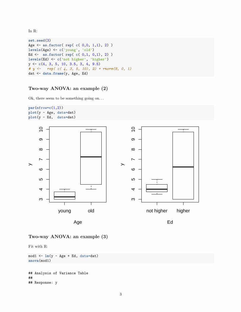
Two-way ANOVA: an example (3)
Fit with R:
mod1 <- lm(y ~ Age + Ed, data=dat)anova(mod1)
## Analysis of Variance Table#### Response: y
3
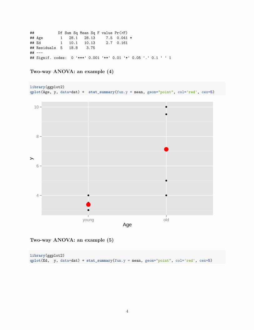
## Df Sum Sq Mean Sq F value Pr(>F)## Age 1 28.1 28.13 7.5 0.041 *## Ed 1 10.1 10.13 2.7 0.161## Residuals 5 18.8 3.75## ---## Signif. codes: 0 '***' 0.001 '**' 0.01 '*' 0.05 '.' 0.1 ' ' 1
Two-way ANOVA: an example (4)
library(ggplot2)qplot(Age, y, data=dat) + stat_summary(fun.y = mean, geom="point", col='red', cex=5)
4
6
8
10
young oldAge
y
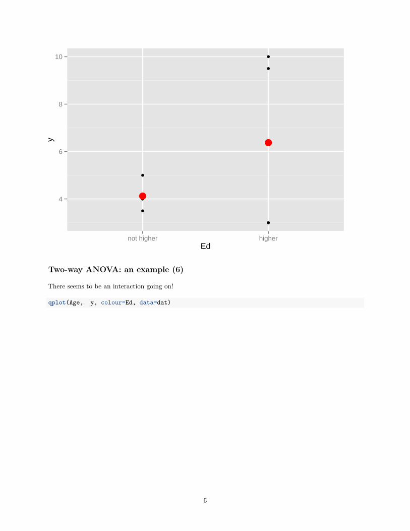
Two-way ANOVA: an example (5)
library(ggplot2)qplot(Ed, y, data=dat) + stat_summary(fun.y = mean, geom="point", col='red', cex=5)
4
4
6
8
10
not higher higherEd
y
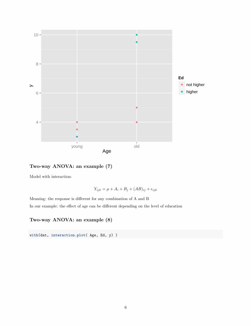
Two-way ANOVA: an example (6)
There seems to be an interaction going on!
qplot(Age, y, colour=Ed, data=dat)
5
4
6
8
10
young oldAge
y
Ed
not higher
higher
Two-way ANOVA: an example (7)
Model with interaction:
Yijk = µ+Ai +Bj + (AB)ij + εijk
Meaning: the response is different for any combination of A and B
In our example: the effect of age can be different depending on the level of education
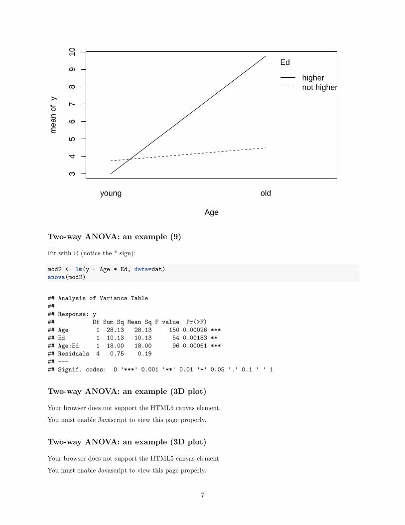
Two-way ANOVA: an example (8)
with(dat, interaction.plot( Age, Ed, y) )
6
34
56
78
910
Age
mea
n of
y
young old
Ed
highernot higher
Two-way ANOVA: an example (9)
Fit with R (notice the * sign):
mod2 <- lm(y ~ Age * Ed, data=dat)anova(mod2)
## Analysis of Variance Table#### Response: y## Df Sum Sq Mean Sq F value Pr(>F)## Age 1 28.13 28.13 150 0.00026 ***## Ed 1 10.13 10.13 54 0.00183 **## Age:Ed 1 18.00 18.00 96 0.00061 ***## Residuals 4 0.75 0.19## ---## Signif. codes: 0 '***' 0.001 '**' 0.01 '*' 0.05 '.' 0.1 ' ' 1
Two-way ANOVA: an example (3D plot)
Your browser does not support the HTML5 canvas element.
You must enable Javascript to view this page properly.
Two-way ANOVA: an example (3D plot)
Your browser does not support the HTML5 canvas element.
You must enable Javascript to view this page properly.
7
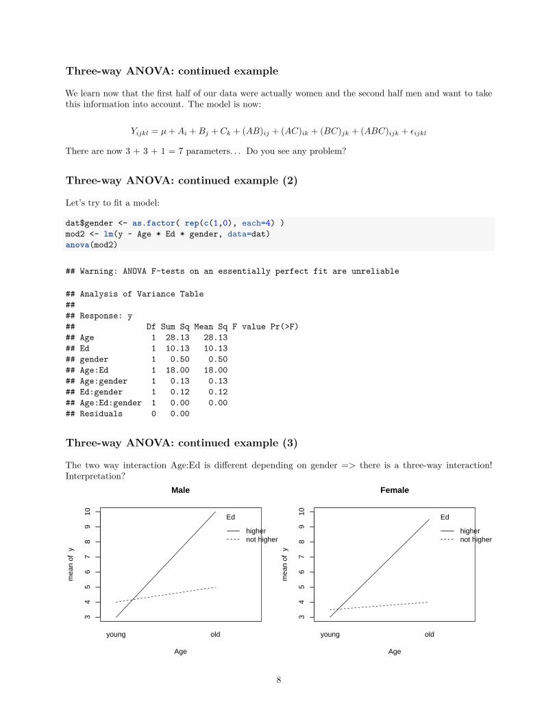
Three-way ANOVA: continued example
We learn now that the first half of our data were actually women and the second half men and want to takethis information into account. The model is now:
Yijkl = µ+Ai +Bj + Ck + (AB)ij + (AC)ik + (BC)jk + (ABC)ijk + εijkl
There are now 3 + 3 + 1 = 7 parameters. . . Do you see any problem?
Three-way ANOVA: continued example (2)
Let’s try to fit a model:
dat$gender <- as.factor( rep(c(1,0), each=4) )mod2 <- lm(y ~ Age * Ed * gender, data=dat)anova(mod2)
## Warning: ANOVA F-tests on an essentially perfect fit are unreliable
## Analysis of Variance Table#### Response: y## Df Sum Sq Mean Sq F value Pr(>F)## Age 1 28.13 28.13## Ed 1 10.13 10.13## gender 1 0.50 0.50## Age:Ed 1 18.00 18.00## Age:gender 1 0.13 0.13## Ed:gender 1 0.12 0.12## Age:Ed:gender 1 0.00 0.00## Residuals 0 0.00
Three-way ANOVA: continued example (3)
The two way interaction Age:Ed is different depending on gender => there is a three-way interaction!Interpretation?
34
56
78
910
Male
Age
mea
n of
y
young old
Ed
highernot higher
34
56
78
910
Female
Age
mea
n of
y
young old
Ed
highernot higher
8
Series 3, exercise 1
In exercise 1 we have two factors (A and B) with 3 levels each. You are asked to estimate the effects Ai, Bj
as well as the interaction ˆ(AB)ij . In this case there is no replica (k = 1).
Remember that Ai = yi·· and ˆ(AB)ij = yij· − (µ+ Ai + Bj)
Series 3, exercise 2
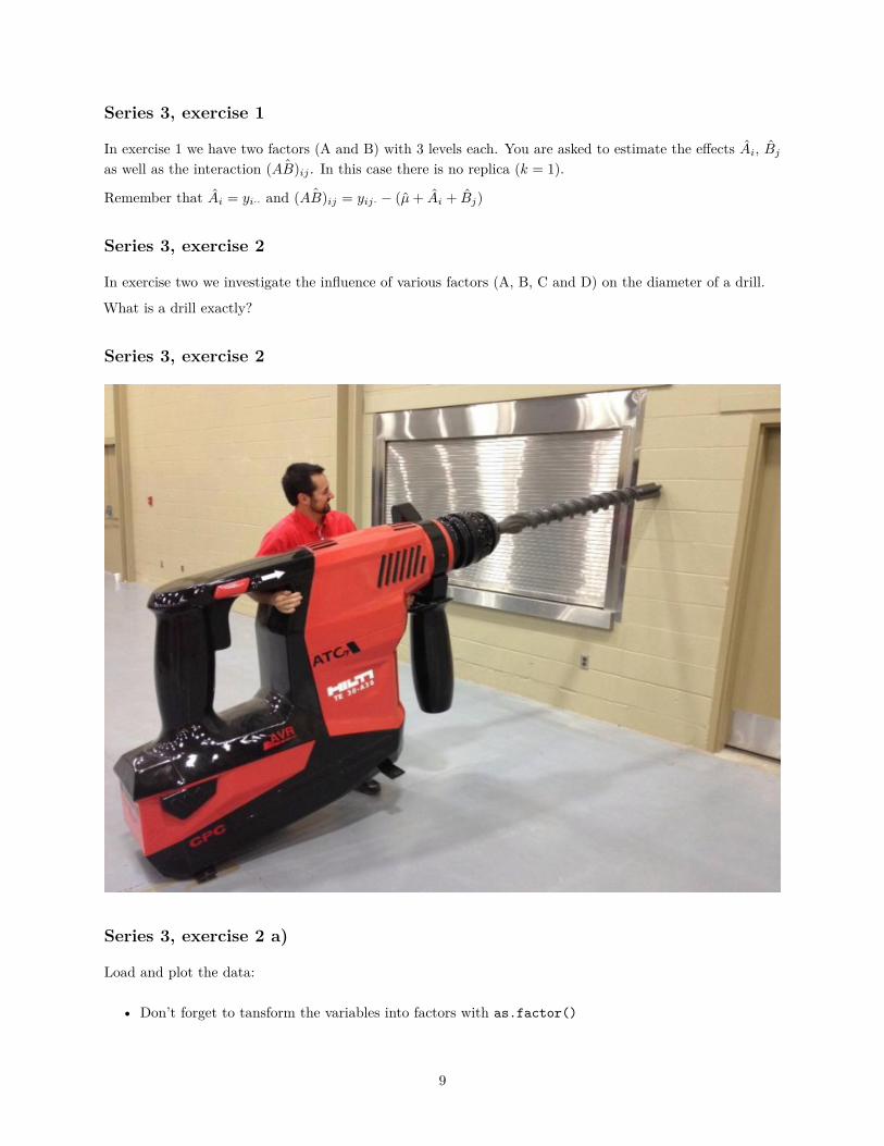
In exercise two we investigate the influence of various factors (A, B, C and D) on the diameter of a drill.
What is a drill exactly?
Series 3, exercise 2
Series 3, exercise 2 a)
Load and plot the data:
• Don’t forget to tansform the variables into factors with as.factor()
9
Series 3, exercise 2 b)
Fit all the interactions:
• To do that, use R formula: Y ~ A*B*C*D
• How many parameters are there in the model? (each factor has two levels)
• main effects: 4• two-way interactions (A:B, A:C, B:C, etc): 4!/2!/2! = 6• three-way interactions (A:B:C, A:B:D, etc): 4!/3!/1! = 4• etc.
• How many data points do you have ? is there a problem?
Series 3, exercise 2 c)
Fit a model with main effects and two-way interactions only:
• To do that, use R formula: Y ~ (A+B+C+D)ˆ2
Series 3, exercise 2 d)
Check the residuals and improve the model if necessary:
• plot( aov(...) )
• If residuals get bigger with bigger fitted value: heteroscedasticity
• Possible solution: log transform the outcome.
Series 3, exercise 3
Here we want to study the influence of sugar, carbonation, sirup and temperature on the quality of a soda.Every combination of factors is tested twice.
• What type of design is it?
• Try to plot interesting interactions.
Series 3
• Any question?
• Thank you!
Thank you!
10
Related Documents