Addis Ababa Institute of Technology School of Electrical and Computer Engineering Anomaly Detection of LTE Cells using KNN Algorithms: The Case of Addis Ababa By Teweldebrhan Mezgebo Advisor Beneyam Berehanu Haile (PhD) A Thesis Submitted to the School of Graduate Studies of Addis Ababa University in Partial Fulfillment of the Requirements for the Degree of Master of Science in Telecommunication Network Engineering. December 2019, Addis Ababa, Ethiopia

Welcome message from author
This document is posted to help you gain knowledge. Please leave a comment to let me know what you think about it! Share it to your friends and learn new things together.
Transcript

Addis Ababa Institute of Technology
School of Electrical and Computer Engineering
Anomaly Detection of LTE Cells using KNN
Algorithms:
The Case of Addis Ababa
By
Teweldebrhan Mezgebo
Advisor
Beneyam Berehanu Haile (PhD)
A Thesis Submitted to the School of Graduate Studies of Addis Ababa University in Partial
Fulfillment of the Requirements for the Degree of Master of Science in Telecommunication
Network Engineering.
December 2019,
Addis Ababa, Ethiopia
Anomaly Detection of LTE Cells Using KNN Algorithms Page i
Addis Ababa Institute of Technology
School of Electrical and Computer Engineering
Anomaly Detection of LTE Cells using KNN
Algorithms:
The Case of Addis Ababa
By
Teweldebrhan Mezgebo
Approval by Board of Examiners
____________
Dean, School of Electrical and Computer Engineering Signature
Beneyam Berehanu Haile (PhD) ____________
Advisor Signature
_______________________ ____________
Examiner Signature
__________________________ ____________
Examiner Signature

Anomaly Detection of LTE Cells Using KNN Algorithms Page ii
Declaration
I, the undersigned, declare that this thesis is my original work, has not been
presented for a degree in this or any other university, and all sources of materials
used for the thesis have been fully acknowledged.
Name: Teweldebrhan Mezgebo
Signature: _____________
Place: Addis Ababa, Ethiopia
Date of Submission:
This thesis has been submitted for examination with my approval as a university
advisor.
Beneyam Berhanu Haile (PhD)
Advisor
Anomaly Detection of LTE Cells Using KNN Algorithms Page iii
Abstract
For mobile operators, delivering quality service to their customers is very important as service
quality significantly affects their business. To achieve a consistent quality service delivery, they
need to continuously monitor and analyze their network performance and timely address any
obtained performance drops. Performance drops in mobile networks can be observed in key
performance indicators (KPIs) of spatially distributed cells with different magnitude and at
different time periods. As it is practically difficult to address all performance drops simultaneously,
it is preferable to make prioritized corrective actions starting from cells with critical drops, also
called anomaly cells. To detect anomaly cells, different automated methodologies have been
proposed and analyzed.
Yet, ethio telecom still applies manual and subjective anomaly detection method where measured
KPI values are manually compared with fixed thresholds to determine if the measured values are
within defined required ranges or not. Cells with KPI values out of the required range are analyzed
for identifying performance drop root causes and taking corrective actions. The manual and
subjective anomaly detection method is prone to detection errors and is maintenance time,
manpower and then cost inefficient. These challenges of manual and subjective detection can be
improved by applying advanced automatic methods based on machine learning algorithms.
In this thesis work, KNN based anomaly detection algorithms such as KNN classification, local
outlier factor (LOF) and connectivity outlier factor (COF) anomaly detection models is
implemented, and their comparative evaluation are made for Addis Ababa LTE cells. The
comparison is made based on type of output, complexity and their true positive rate (TPR) for time
series and cell level detections. Unlike KNN classification, LOF and COF do not need heavy data
set training and are able to provide anomaly scores instead of two-class labels. Experimentation
results show that COF provides slightly better performance than the other models with negligible
performance difference. For instance, the performance of COF with respect to TPR for RRC setup
success rate in the experimentation is 97.91% for cell level detection and 88% for time series
detection.
Key words: Anomaly detection, Connectivity outlier factor, Local outlier factor, KNN classification,
Machine Learning, KPI, Alarm, LTE

Anomaly Detection of LTE Cells Using KNN Algorithms Page iv
Acknowledgments
First, I would like to express my gratitude to the almighty God and to Saint Mary
mother of God, who let me stay healthy and has enabled me to work hard physically,
mentally & spiritually for the completion of this thesis work.
I would like to thank my advisor Dr. Beneyam Berehanu for his invaluable support,
advices and follow up throughout the research. His motivational ideas and positive
attitude enabled me to work hard. It would have been difficult to complete the thesis
without his continuous guidance.
I would like to give credit to my wife for her continuous support and motivation
towards my thesis work. She was amazing in tolerating and solving challenges.
Especially the way she helped me during my illness while she needed support being
pregnant and in delivery is unforgettable.
I also would like to express my gratitude to Filimon Tesfahunegn and Tesfay
G/giorgis who have spent continues sleepless nights in hospital to save my life when
I was ill in the middle of my thesis work. My sincere thanks goes to ethio telecom for
its sponsorship to attend my masters class covering all important facilities.
I am very much thankful to Tsegay Woldeyohanis, Kelem Alemu, Tsehaynesh
Ashebir, Tewodros Belay and Dawit Kefalegn for their invaluable support in
providing important data for my thesis work.

Anomaly Detection of LTE Cells Using KNN Algorithms Page v
Table of Content
Abstract ........................................................................................................................ iii
Acknowledgments ......................................................................................................... iv
List of Tables ................................................................................................................. ix
List of Acronyms ............................................................................................................ x
1. Introduction ............................................................................................................. 1
1.1 Background & Motivation ................................................................................ 1
1.2 Statement of the Problem ................................................................................. 3
1.3 Objectives .......................................................................................................... 3
1.3.1 General Objective ....................................................................................... 3
1.3.2 Specific Objectives ...................................................................................... 4
1.4 Methodology ...................................................................................................... 4
1.5 Related Work .................................................................................................... 5
1.6 Scope and Limitation of the Thesis .................................................................. 7
1.7 Contribution of the Thesis ................................................................................ 7
1.8 Thesis Structure ............................................................................................... 7
2 LTE KPIs and Performance Anomaly .................................................................... 8
2.1 LTE Network Architecture ............................................................................... 9
2.2 LTE KPIs ........................................................................................................ 12
2.2.1 LTE KPI Parameters ............................................................................... 15
2.2.2 Impact of Alarms in LTE Cells KPI ........................................................ 16
2.3 Anomaly in LTE KPIs .................................................................................... 17
2.3.1 Types of Anomaly ..................................................................................... 17
2.3.2 Root Causes of Performance Anomaly .................................................... 20
Anomaly Detection of LTE Cells Using KNN Algorithms Page vi
3 Anomaly Detection Methods ................................................................................. 22
3.1 Classification of Anomaly Detection Methods ............................................... 22
3.1.1 Nature of Input Data ............................................................................... 22
3.1.2 Outputs of Anomaly Detection ................................................................ 23
3.1.3 Distribution of Input Data Sets ............................................................... 23
3.1.4 Availability of Supervision ...................................................................... 24
3.2 Challenges of Anomaly Detection .................................................................. 25
3.3 Application Areas of Anomaly Detection ....................................................... 26
4 Anomaly Detection in Addis Ababa LTE KPIs .................................................... 27
4.1 LTE KPI Measurement .................................................................................. 28
4.2 LTE Worst Performing Cells Selection & Analysis ....................................... 29
5 KNN-based Anomaly Detection Techniques ........................................................ 32
5.1 Assumptions .................................................................................................... 33
5.2 KNN Classification System Model ................................................................. 33
5.2.1 Mathematics of KNN Classification ........................................................ 34
5.3 Density-based Local Outlier Factor ............................................................... 37
5.3.1 System Model of Local Outlier Factor ..................................................... 37
5.3.2 Mathematics of Local Outlier Factor ...................................................... 38
5.4 Connectivity Outlier Factor ........................................................................... 40
5.4.1 Mathematics of Connectivity Outlier Factor .......................................... 41
5.5 Performance Evaluation Mechanisms of Anomaly Detection ....................... 42
6 Experimentation and Result Analysis ................................................................. 44
6.1 Data Collection and Preprocessing ................................................................ 44
6.1.1 Distribution Fitting .................................................................................. 44
Anomaly Detection of LTE Cells Using KNN Algorithms Page vii
6.1.2 Data Set Labeling Result ......................................................................... 46
6.2 Results with KNN Classification ................................................................... 47
6.3 Results with Local Outlier Factor .................................................................. 48
6.4 Result with Connectivity Outlier Factor ....................................................... 50
6.5 Performance Comparison and Discussion ..................................................... 54
7 Conclusion and Future Work ................................................................................ 57
7.1 Conclusion ....................................................................................................... 57
7.2 Future Work.................................................................................................... 57
References .................................................................................................................... 58
Anomaly Detection of LTE Cells Using KNN Algorithms Page viii
List of Figures
Figure 1-1 LTE Cells KPI Monitoring Architecture ...................................................................... 2
Figure 2-1 LTE Network Architecture ............................................................................................. 9
Figure 2-2 RRC Connection Setup Process ................................................................................. 14
Figure 2-3 E-RAB Setup Success Process ..................................................................................... 14
Figure 2-4 Definition of Anomaly .................................................................................................. 17
Figure 2-5 Point Anomaly ............................................................................................................... 18
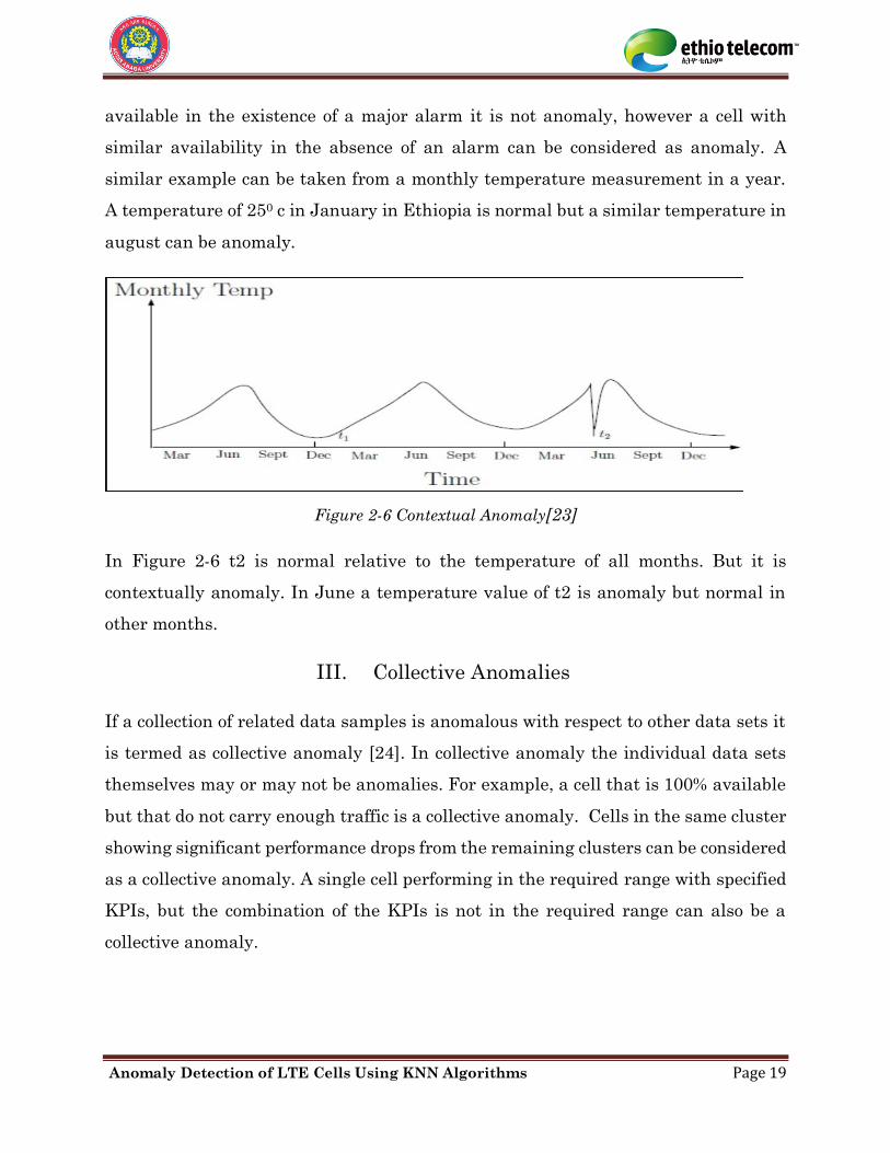
Figure 2-6 Contextual Anomaly ...................................................................................................... 19
Figure 2-7 Collective Anomaly ........................................................................................................ 20
Figure 3-1 Modes of Anomaly Detection on Availability of Labeled Data Set ......................... 25
Figure 4-1 Manual Worst Cell Selection vs Automatic Anomaly Detection ............................ 30
Figure 5-1 General Framework of Anomaly Detection ............................................................... 32
Figure 5-2 KNN Classification Process Model .............................................................................. 33
Figure 5-3 Process Model of LOF and COF................................................................................... 38
Figure 5-4 K-distance of a Point ..................................................................................................... 38
Figure 5-5 Difference between COF and LOF .............................................................................. 40
Figure 6-1 RRC Setup Success Rate Distribution Fitting .......................................................... 45
Figure 6-2 SDR Distribution Fitting .............................................................................................. 45
Figure 6-3 Cell Level data Set Labeling ........................................................................................ 46
Figure 6-4 Time Series Data Set Labeling .................................................................................... 46
Figure 6-5 Cell Level RRC Success Anomaly Detection with KNN Classification ................. 47
Figure 6-6 Anomaly Score of Cell Level RRC Setup Success Rate using LOF ........................ 49
Figure 6-7 Cell level RRC Setup Success Rate Anomaly Detection with LOF ........................ 49
Figure 6-8 Time Series Anomaly Detection with LOF ................................................................ 50
Figure 6-9 Anomaly Score of RRC Setup Success Rate with COF ............................................ 51
Figure 6-10 Cell Level RRC Setup Success Rate Anomaly Detection with COF .................... 51
Figure 6-11 Time Series Anomaly Detection with COF for Hourly SDR Data........................ 52
Figure 6-12 Cell Level SDR Anomaly Detection with COF ........................................................ 53
Figure 6-13 Cell Level E-RAB Setup Anomaly Detection with COF ........................................ 53
Figure 6-14 Anomaly Interdependence among Different KPI Metrices ................................... 54
Figure 6-15 Performance Comparison of Anomaly Detection Models....................................... 55
Anomaly Detection of LTE Cells Using KNN Algorithms Page ix
List of Tables
Table 2-1 LTE Standard Versions .................................................................................................... 8
Table 2-2 LTE RAN KPIs Categorization According to 3GPP .................................................. 12
Table 4-1 Sample KPI Requirement Range in ethio telecom .................................................... 27
Table 6-1 Confusion Matrix for Cell Level KNN Classification ................................................ 48
Table 6-2 Confusion Matrix of Time Series KNN Classification .............................................. 48

Anomaly Detection of LTE Cells Using KNN Algorithms Page x
List of Acronyms
3GPP 3rd generation partnership project
AUC Area under ROC curve
COF Connectivity outlier factor
EPC Evolved packet core
E-RAB Evolved radio access bearer
EWMA Exponentially weighted moving average
FPR False positive rate
FNR False negative rate
HSPA High speed packet access
HSS Home subscription server
IS Information system
KNN K nearest neighbours
KPI Key performance indicator
LOF Local outlier factor
LTE Long term evolution
MME Mobility management entity
MNO Mobile network operator
NMS Network management system
PCC Policy and charging control
PCRF Policy and charging resource function
P-GW Packet data network gateway
PRB Physical resource block
PRS Performance record system
PS Packet switch
QoS Quality of service
RAN Radio access network
ROC Region of convergence
RRC Radio resource control

Anomaly Detection of LTE Cells Using KNN Algorithms Page xi
RRU Radio resource unit
SAE System architecture evolution
SDR Service drop rate
S-GW Serving gateway
SLA Service level agreement
SMC Service management center
SON Self-organized networks
SPC Statistical process control
TS Time series
TNR True negative rate
TPR True positive rate
UE User equipment
VoIP Voice over internet protocol
Anomaly Detection of LTE Cells Using KNN Algorithms Page 1
1. Introduction
1.1 Background and Motivation
Today, where subscribers need seamless connectivity anywhere and anytime,
increasing base stations for providing adequate capacity and coverage is not enough.
Thus, mobile operators need to timely monitor their network and work on quality of
service assurance for providing granted quality of service to customers. However, the
changing dynamics of radio network features and metrics pose challenges for
operators in terms of optimizing and maximizing network efficiency while reducing
operational expenditure [1]. According to [2] radio access network (RAN)
organizations are always in need of quick answers to the following questions:
▪ Is there an easier way of sensing the performance and quality of a RAN
network?
▪ Is there a more efficient way to detect and compensate for service
performance drops?
Globally, competition in the liberalized telecommunications markets and the
requirements of customers for more complex services are leading to a greater
emphasis on quality of service automation [1]. To prevent fault and outage early
before they possibly occur it is important that the detection and localization of
anomaly cells should be as fast as possible. The efficiency of anomaly detection
determines the quality of taking corrective actions for performance drop recovery. To
realize network monitoring automation operators are moving towards self-organized
networks (SON) self-healing functionalities to detect and fix network faults [3-5].
In ethio telecom network monitoring is done on equally spaced time intervals
(monthly, weekly, daily and hourly) for all cells as shown in Figure 1-1. The
performance values queried from performance recording systems (PRS) mostly
depend on the configuration quality in the U2000 server and the quality of
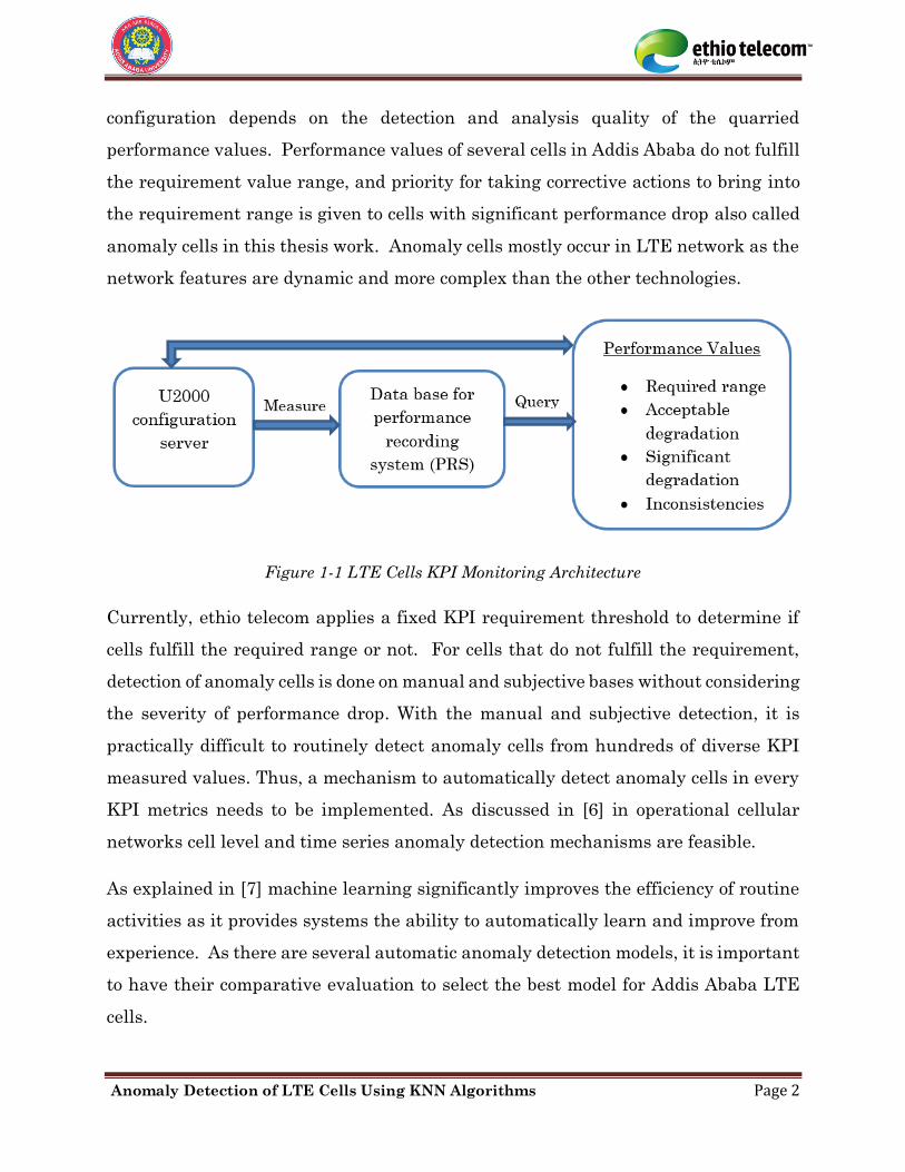
Anomaly Detection of LTE Cells Using KNN Algorithms Page 2
configuration depends on the detection and analysis quality of the quarried
performance values. Performance values of several cells in Addis Ababa do not fulfill
the requirement value range, and priority for taking corrective actions to bring into
the requirement range is given to cells with significant performance drop also called
anomaly cells in this thesis work. Anomaly cells mostly occur in LTE network as the
network features are dynamic and more complex than the other technologies.
Figure 1-1 LTE Cells KPI Monitoring Architecture
Currently, ethio telecom applies a fixed KPI requirement threshold to determine if
cells fulfill the required range or not. For cells that do not fulfill the requirement,
detection of anomaly cells is done on manual and subjective bases without considering
the severity of performance drop. With the manual and subjective detection, it is
practically difficult to routinely detect anomaly cells from hundreds of diverse KPI
measured values. Thus, a mechanism to automatically detect anomaly cells in every
KPI metrics needs to be implemented. As discussed in [6] in operational cellular
networks cell level and time series anomaly detection mechanisms are feasible.
As explained in [7] machine learning significantly improves the efficiency of routine
activities as it provides systems the ability to automatically learn and improve from
experience. As there are several automatic anomaly detection models, it is important
to have their comparative evaluation to select the best model for Addis Ababa LTE
cells.
Anomaly Detection of LTE Cells Using KNN Algorithms Page 3
1.2 Statement of the Problem
The manual and subjective anomaly detection method in ethio telecom consumes
maintenance time and manpower and, hence, is cost inefficient. As the performance
of several cells in different KPI metrics do not meet the fixed requirement threshold
and it is practically difficult to fix all the cells in all metrics simultaneously, the
manual and subjective detection faces difficulty in prioritizing cells for corrective
actions. Thus, anomalies remain unfixed for a longer time and they become a cause
for anomalies of higher magnitude and complete network outages. The manual
detection process is prone to errors, thus detected anomalies raise questions of
credibility in different regions of the company and sometimes become a source of
conflict between departments.
In summary, the main problems are,
• The hard and fixed KPIs threshold does not consider the dynamic nature of
cells as it is fixed.
• The current manual detection is done based on current performance values
and faces difficulty to include history performance values.
• The manual anomaly detection is maintenance time, manpower and then cost
inefficient.
• The manual anomaly detection method is prone to errors, thus it may lead to
wrong analysis and let anomalies to remain unfixed.
1.3 Objectives
1.3.1 General Objective
The general objective of this thesis work is to present performance comparison and
implementation of machine learning algorithms for automatic detection of anomaly
cells for Addis Ababa LTE network.
Anomaly Detection of LTE Cells Using KNN Algorithms Page 4
1.3.2 Specific Objectives
The specific objectives of the thesis are
▪ Undertake performance comparison of anomaly detection algorithms for Addis
Ababa LTE cells.
▪ Select and implement most suitable machine learning algorithms for cell level
and time series anomaly detection of LTE cells in Addis Ababa.
▪ Present the most anomaly cells for selected KPIs along with their anomaly
score and occurrence time.
1.4 Methodology
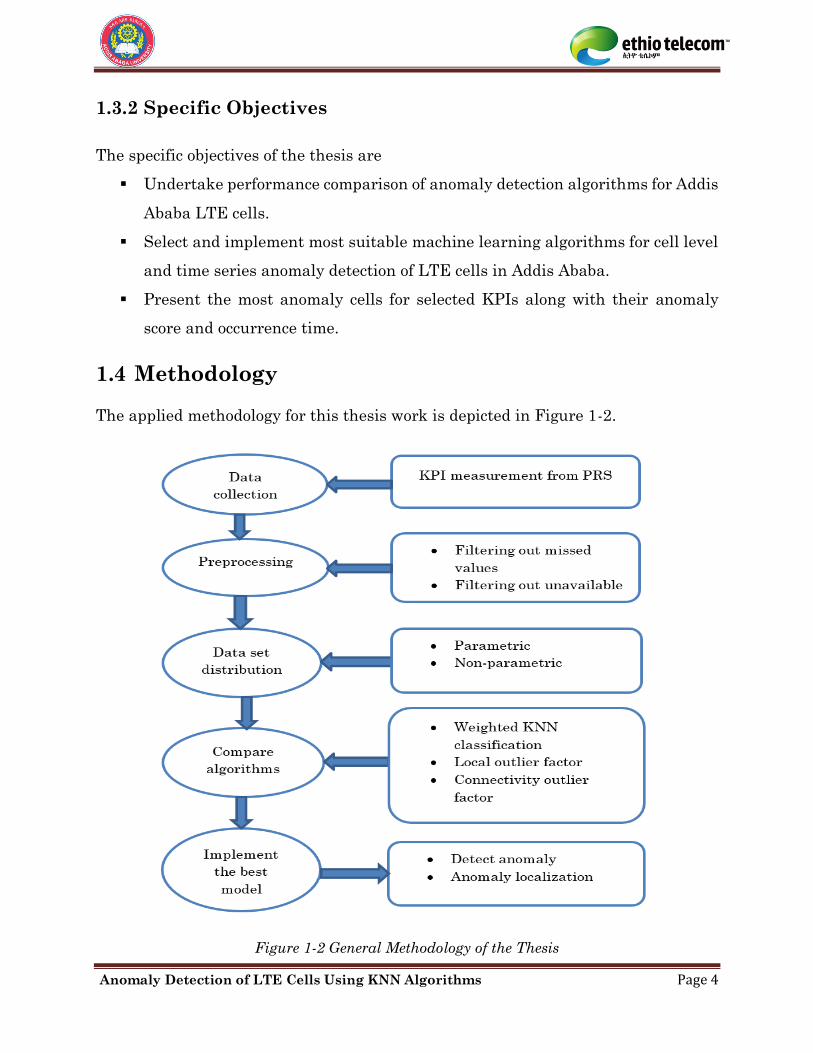
The applied methodology for this thesis work is depicted in Figure 1-2.
Figure 1-2 General Methodology of the Thesis

Anomaly Detection of LTE Cells Using KNN Algorithms Page 5
The detection work starts with collection of LTE cells performance data. Because it
is practically difficult to have experimentation for all KPIs RRC setup success rate,
E-RAB setup success rate and service drop rate KPI metrics are collected as a sample
raw data.
After collecting the data, preprocessing work is done to filter out inconsistent values.
The algorithms that can be applied accept numeric values only and missed values
should be filtered out. Because performance drops due to power outage, alarms and
transmission cut should not be considered as anomalies, performance values of cells
with alarms and unavailable cells are also filtered out.
For there are several anomaly detections models, model comparison is done
considering different criteria and the best model is accordingly selected.
Implementation of different algorithms that are based on the best model,
performance evaluation and comparison of the algorithms is done using Matlab as a
tool.
1.5 Related Work
Performance anomalies in LTE cells occur due to several reasons. One of the main
causes of an anomaly in mobile networks is an error in feature configuration and
parameter change.
In [1] a configuration management assessment method for a SON in mobile networks
using a two-sample Kolmogorov-Smirnov test is explained. The authors in [1]
collected RRC setup success rate, E-RAB setup success rate, inter eNodeB handover
success rate and cell availability of 1230 eNodeBs from a network management
system (NMS) as a raw data. The authors noted that not all configuration changes
bring a positive result and some configuration changes can lead even to a worse
performance drop. Their focus is to give recommendations to undo or accept the
corresponding configuration changes. However, the methodology the authors followed
shows a two class (normal or anomaly) labeled result, and hence it is difficult to have
Anomaly Detection of LTE Cells Using KNN Algorithms Page 6
the degree of anomaly and evaluate the severity of performance drops with the
corresponding KPI metrics.
There are several types of anomaly detection algorithms that are applied to different
data set types. These algorithms are different for different services (voice, data,
image) and for different data set distribution types (parametric and non-parametric).
In [9] comparison of different anomaly detection algorithms is clearly explained and
recommends the preferred anomaly detection model for different data set types and
purposes. The focus of [9] is to compare unsupervised anomaly detection algorithms
for different services. The paper clearly explained and compared KNN-based,
clustering-based, statistical-based, subspace-based and classifier-based anomaly
detection algorithms, but none of them is implemented for LTE KPIs data.
In [6][10] it is explained that no single model can accurately detect all anomalies in
mobile network performance. The papers focus on the problem of cell anomaly
detection, addressing partial and complete degradations in cell-service performance,
and they implemented an adaptive ensemble method framework for modeling cell
behavior. The framework uses key performance indicators (KPIs) to determine cell-
performance status and control legitimate system configuration changes.
In [11] cell outage detection via handover success rate anomaly detection in UMTS
networks is discussed. The author applied density-based local outlier factor for the
anomaly detection and percentile-based threshold setting by preparing a reference
value at first. The paper has not explained the degree of the service outage and could
not indicate if the outages are performance drop or complete failures. The author has
not also explained how exactly the initial reference threshold values are set.
Several other related works are done. However, to the best of my knowledge cell level
and time series anomaly detection algorithm that considers spatial and temporal
proximity and is more suitable for Addis Ababa LTE network KPIs is not studied and
selected, while demonstrating the feasibility of operational deployment.

Anomaly Detection of LTE Cells Using KNN Algorithms Page 7
1.6 Scope and Limitation of the Thesis
The scope of the thesis is to compare and implement KNN-based anomaly detection
methods for Addis Ababa LTE cells for cell level and time series scenarios.
The limitation of the thesis is that anomaly detection experimentation is done for
selected KPI metrics and not for all. Thus, anomaly detection of cells from KPIs that
can be measured with a driving test is not included in both scenarios.
1.7 Contribution of the Thesis
This research work presents the following two major contributions:
▪ It provides comparative analysis of KNN algorithms for anomaly detection in
the context of Addis Ababa LTE network and can supports operators to select
the most appropriate anomaly detection model for their network.
▪ It provides the directions and methodologies for automating the current
manual anomaly detection approach. This automation can help operators to
enhances service quality and revenue by saving maintenance time, manpower
and then cost. Furthermore, it presents better data insights and avoids human
errors and thus bring better credibility in reporting.
1.8 Thesis Structure
The thesis is organized as follows:
Chapter two presents a theoretical background on LTE networks, LTE KPIs and
anomalies. Chapter three presents basics of anomaly detection methods and anomaly
detection classification aspects. Chapter four discusses anomaly detection in the case
of Addis Ababa LTE network and the limitations of the current detection mechanism
applied in ethio telecom. Chapter five is about KNN-based anomaly detection
methods and their mathematical models. Experimentation of data sets and result
analysis along with performance evaluation of the algorithms are discussed in
Chapter six. Finally, Chapter seven deals with conclusion and future work.
Anomaly Detection of LTE Cells Using KNN Algorithms Page 8
2 LTE KPIs and Performance Anomaly
According to [13] LTE is defined as a new packet-only wideband radio with flat
architecture technology developed to get enhanced capacity, reduced service latency,
increased data rate and lower cost data delivery than previously developed GSM and
UMTS services. The initial assumption during development was that LTE will have
a peak downlink data rate of 100Mbps and uplink data rate of 50Mbps with a round
trip time (RTT) latency of 10ms. LTE uses orthogonal frequency division multiple
access (OFDMA) in downlink and single carrier frequency division multiple access
(SC-FDMA) in uplink as multiple access. Resource allocation in the frequency domain
takes place with a resolution of 180 kHz resource blocks called physical resource
blocks (PRB) both in uplink and in downlink. Resources are allocated based on
different scheduling techniques.
The work towards LTE started in 2004 and is continuously evolving [13][14]. LTE
standards are delivered in rolling versions or releases. The first LTE standard is
Release 8, that could deliver a downlink data rate of 150Mbps and uplink data rate
of 75Mbps which is higher than the target set. According to [13] 3GPP standardized
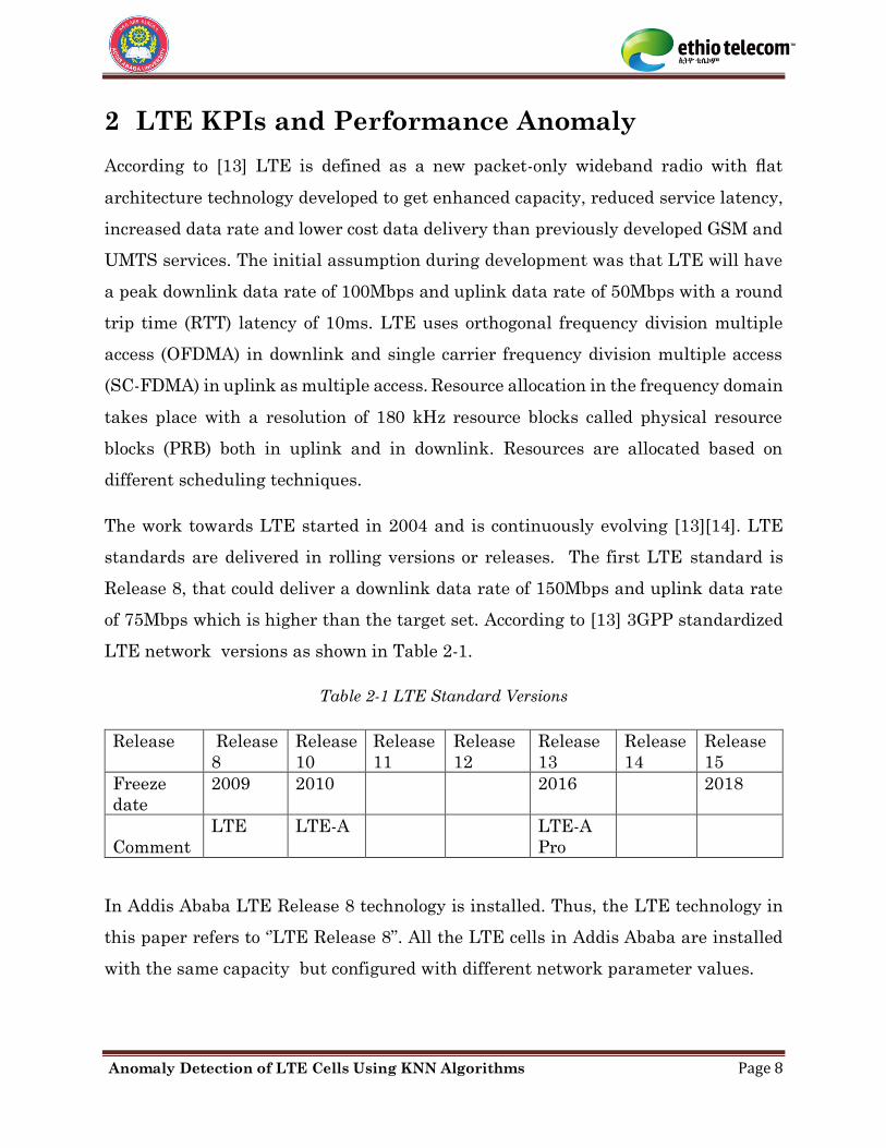
LTE network versions as shown in Table 2-1.
Table 2-1 LTE Standard Versions
Release Release
8
Release
10
Release
11
Release
12
Release
13
Release
14
Release
15
Freeze
date
2009 2010 2016 2018
Comment
LTE LTE-A LTE-A
Pro
In Addis Ababa LTE Release 8 technology is installed. Thus, the LTE technology in
this paper refers to ‘’LTE Release 8”. All the LTE cells in Addis Ababa are installed
with the same capacity but configured with different network parameter values.

Anomaly Detection of LTE Cells Using KNN Algorithms Page 9
2.1 LTE Network Architecture
The service quality delivered is determined by different network elements and
interfaces between them. The fact that KPI as a measure of service quality needs to
be end to end (from the mobile user equipment to the core elements), it is important
to see how the different network components are linked and interconnected.
According to [13] the LTE network architecture that includes the network elements
along with the interfaces looks as shown in Figure 2-1.
Figure 2-1 LTE Network Architecture[13]
As can be seen in Figure 2-1 there are several LTE network elements and
components. By referring to books in [13] and [14] the description of LTE components
is explained as,
I. User Equipment
The user equipment (UE) is the device that the end user uses for communication.
Typically, it is a handheld device such as a smart phone or a data card or it could be
embedded, e.g. to a laptop. UE also contains the universal subscriber identity module
(USIM) which is a separate module from the rest of the UE, which is often called the
Terminal equipment (TE). USIM is used to identify and authenticate the user and to
derive security keys for protecting the radio interface transmission. Functionalities
Anomaly Detection of LTE Cells Using KNN Algorithms Page 10
that include mobility management functions such as handovers and reporting the
terminal’s location are supported by the user equipment.
II. E-UTRAN Node B
E-UTRAN NodeB (eNodeB) is a radio base station that is in control of all radio related
functions in the fixed part of the system. eNodeBs are typically distributed
throughout the network’s coverage area, each eNodeB residing near the actual radio
antennas. Functionally eNodeBs acts as a layer 2 bridge between UE and evolved
packet core (EPC), by being the termination point of all the radio protocols towards
the UE. In this role, the eNodeB performs ciphering and deciphering of data, IP
header compression and decompression, which means avoiding repeatedly sending
the same or sequential data in an IP header. The eNodeB is responsible for and has
an important role in radio resource management, mobility management, bearer
handling, user plane data delivery, securing and optimizing radio interface delivery.
III. Mobility Management Entity
Mobility management entity (MME) is the main control element in the EPC.
Typically, the MME would be a server in a secure location in the operator’s premises.
It operates only in the control plane and is not involved in the path of user plane data.
The main MME functions include authentication and security, mobility management,
managing subscription profile and service connectivity.
IV. Serving Gateway
Serving gateway (S-GW) is part of the network infrastructure maintained centrally
in operation premises for user plane tunnel management and switching. The S-GW
has a very minor role in control functions. It is only responsible for its own resources,
and it allocates them based on requests from MME, P-GW or PCRF, which in turn
are acting on the need to set up, modify or clear bearers for the UE.
Anomaly Detection of LTE Cells Using KNN Algorithms Page 11
V. Packet Data Network Gateway
Packet data network gateway (P-GW) is the edge router between the EPC and
external packet data networks. It is the highest-level mobility anchor in the system,
and usually it acts as the IP point of attachment for the UE. It performs traffic gating
and filtering functions as required by the service in question. As to the S-GW, the P-
GWs are maintained in operator premises in a centralized location. P-GW is the
highest-level mobility anchor in the system. When a UE moves from one S-GW to
another, the bearers must be switched in the P-GW. The P-GW will receive an
indication to switch the flows from the new S-GW.
VI. Policy and Charging Resource Function
Policy and charging resource function (PCRF) is the network element that is
responsible for policy and charging control (PCC). It makes decisions on how to handle
the services in terms of QoS and provides information to P-GW.
VII. Home Subscription Server
Home subscription server (HSS) is the subscription data repository for all permanent
user data. It also records the location of the user in the level of visited network control
node, such as MME. It is a database server maintained centrally in the home
operator’s premises. There are several interfaces in LTE network, some of the
commonly known standard interfaces are listed below [13][14].
▪ Uu interface is an interface for the control plane and user plane between UE
and eNode B.
▪ X2 interface is an interface for control plane and user plane between two
eNodeBs.
▪ S1-u interface is an interface for the user plane between eNodeBs and S-GW.
▪ S11 interface is an interface for the control plane between MME and S-GW.
▪ S1-MME interface is an interface for the control plane between eNodeBs and
MME.
Anomaly Detection of LTE Cells Using KNN Algorithms Page 12
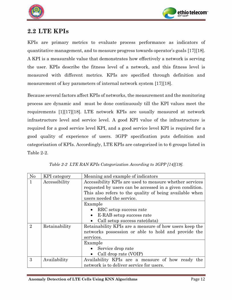
2.2 LTE KPIs
KPIs are primary metrics to evaluate process performance as indicators of
quantitative management, and to measure progress towards operator’s goals [17][18].
A KPI is a measurable value that demonstrates how effectively a network is serving
the user. KPIs describe the fitness level of a network, and this fitness level is
measured with different metrics. KPIs are specified through definition and
measurement of key parameters of internal network system [17][18].
Because several factors affect KPIs of networks, the measurement and the monitoring
process are dynamic and must be done continuously till the KPI values meet the
requirements [1][17][18]. LTE network KPIs are usually measured at network
infrastructure level and service level. A good KPI value of the infrastructure is
required for a good service level KPI, and a good service level KPI is required for a
good quality of experience of users. 3GPP specification puts definition and
categorization of KPIs. Accordingly, LTE KPIs are categorized in to 6 groups listed in
Table 2-2.
Table 2-2 LTE RAN KPIs Categorization According to 3GPP [14][19].
No KPI category Meaning and example of indicators
1 Accessibility Accessibility KPIs are used to measure whether services
requested by users can be accessed in a given condition.
This also refers to the quality of being available when
users needed the service.
Example
• RRC setup success rate
• E-RAB setup success rate
• Call setup success rate(data)
2 Retainability Retainability KPIs are a measure of how users keep the
networks possession or able to hold and provide the
services.
Example
• Service drop rate
• Call drop rate (VOIP)
3 Availability Availability KPIs are a measure of how ready the
network is to deliver service for users.
Anomaly Detection of LTE Cells Using KNN Algorithms Page 13
Example
• Cell availability rate
4 Mobility
Mobility KPIs are a measure of the capability of the
networks service continuity during user’s movement.
Example
• Intra frequency handover success rate
• Inter frequency handover success rate
• IRAT handover success rate
5 Integrity Integrity KPIs are a measure of the networks character
or honesty to its users.
Example:
• Throughput per cell
• Throughput per user
• Latency
6 Utilization Utilization KPIs are a measure of utilization of the
maximum capacity of the network for a specified
resource.
Example:
• UL PRB utilization
• DL PRB utilization
• Power utilization
According to 3GPP there are several other KPIs that are not included in the list in
each category. In this thesis work experimentation is done for RRC setup success
rate, E-RAB setup success rate and service drop rate.
I. RRC Setup Success Rate
RRC is the major part of the control signaling between UE and the network. RRC
messages control all procedures related to establishment and release of connection
including paging. Configuration measurements and reporting for handovers are also
controlled by RRC messages. The main and possible reasons that can be listed for
RRC failure are RRC setup failure due to no response from eNodeB, RRC setup
failure due to eNodeB rejection and failure due to no response from UE after getting
a response from eNodeB. RRC setup success rate is calculated based on the counter
at the eNodeB when the eNodeB received the RRC connection request from UE.
Complete RRC connection setup can be illustrated by the diagram in Figure 2-2.

Anomaly Detection of LTE Cells Using KNN Algorithms Page 14
Figure 2-2 RRC Connection Setup Process [19]
Number of RRC connection attempt is collected by the eNodeB at point A, and the
number of successful RRC connection is calculated at point C.
Connection Setup Complete 100% 100%
RRC Connection Request
RRC CRRC setup success rate
A= = (2-1)
II. E-RAB Setup Success Rate
E-RAB is a protocol to establish a fixed communication path between UE and core
network. It is within a radio access bearer that the network builds up the end-to-end
QoS connection. Bearers in LTE cells are granted or rejected by admission control
algorithm in the E-RAB. E-RAB setup responses can be sent after RRC connection
reconfiguration setup is successful.
Figure 2-3 E-RAB Setup Success Process[19]
Anomaly Detection of LTE Cells Using KNN Algorithms Page 15
E-RAB setup success rate KPI shows the probability of success ERAB to access all
services including VoIP in a cell or radio network. The complete ERAB setup can be
illustrated by the process diagram in Figure 2-3. KPI is calculated based on counter
ERAB connection setup attempt at point A and successful ERAB setup counter at
point B.
III. Service Drop Rate
Service drop rate as KPI indicates the drop rate of all the services in a cell or radio
network, including call drop rate in VoIP service. This KPI measures abnormal
releases at the eNodeB and is equivalent to call drop rate in voice services. The main
causes for performance anomaly in service drop rate are,
▪ Abnormal E-RAB release due to eNodeB
▪ Abnormal E-RAB release due to transmission
▪ Abnormal E-RAB release due to network congestion
▪ Abnormal E-RAB release due to EPC
Re CounterService Drop Rate = 100%
Normal Release + ERAB Abnormal Release
ERAB Abnormal lease
ERAB ( 2-2)
2.2.1 LTE KPI Parameters
The quality of configuration of LTE parameters is critical to bring quality of service.
There are several LTE performance parameters that determine the degree of service
quality. With the dynamic nature of LTE network, the parameters need to be
configured/reconfigured timely to recover any obtained performance drops. However,
the reconfiguration may not always bring a positive result and sometimes a worse
performance in the configured/reconfigured cell can be observed. Thus, quality of
parameter configuration is usually the source of cell performance anomaly with
respect to KPIs that are directly associated or dependent on the parameter to be
configured or reconfigured. Certain configuration in one cell may bring cell
Anomaly Detection of LTE Cells Using KNN Algorithms Page 16
performance anomaly in another cell. Some of the common LTE performance
parameters are listed below.
▪ Resource allocation (uplink and downlink)
▪ Inter-cell interference coordination (ICIC)
▪ Mobility control (Including cell reselection parameters)
▪ Load control (including admission control and random-access control)
▪ Power control (uplink and downlink)
2.2.2 Impact of Alarms in LTE Cells KPI
According to [20] LTE cells need to monitor the status of their hardware and software.
If software or hardware faults are detected by the cell alarms are generated. This
hardware or software faults are usually a cause for significant drops and complete
outages. The hardware and software faults may include faults in radio resource unit
(RRU), baseband processing board (BBP), common public radio interface (CPRI) port,
feeder, power supply system, and transport link. There are several types of alarms,
in [21] alarms are classified in to critical, major, minor and warning according to their
severity. In [21] the alarm categories are defined as,
▪ Critical alarms are the most serious alarms that can interrupt the services and
causes the NE to break down. Critical alarms need to be handled immediately.
▪ Major alarms have minor impacts on certain NEs or system functions and
needs to be handled as soon as possible before they become a cause to disable
important features. This type of alarms can not be a cause for complete system
break down. Cells with major alarms are expected to be with significant
performance drops in the metrics related to the affected features.
▪ Minor alarms indicate for invents that do not have any impact on the Network
elements, but they are an indication that the system detects a potential or
imminent event that may affect services. Their aim is to inform the
maintenance team for future faults.
Anomaly Detection of LTE Cells Using KNN Algorithms Page 17
▪ Warning alarms indicate an event that has no impact on the system functions
and services. However, the event may have potential impacts on future service
quality of NEs or resources.
2.3 Anomaly in LTE KPIs
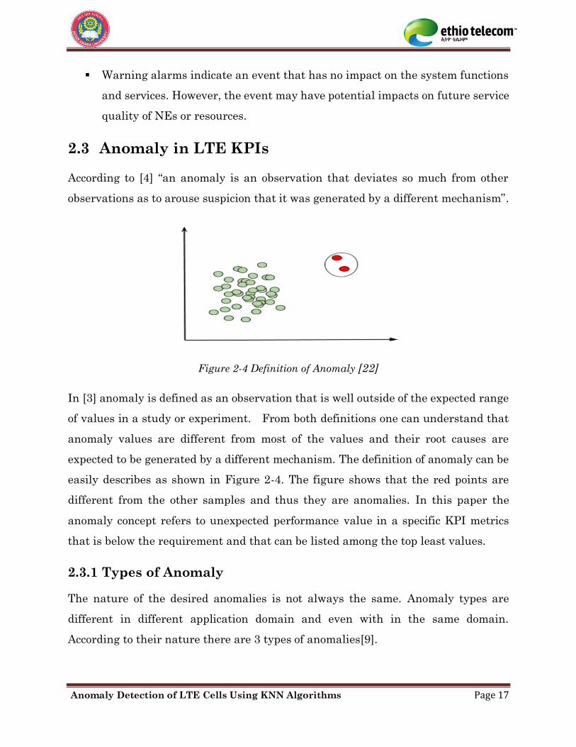
According to [4] “an anomaly is an observation that deviates so much from other
observations as to arouse suspicion that it was generated by a different mechanism”.
Figure 2-4 Definition of Anomaly [22]
In [3] anomaly is defined as an observation that is well outside of the expected range
of values in a study or experiment. From both definitions one can understand that
anomaly values are different from most of the values and their root causes are
expected to be generated by a different mechanism. The definition of anomaly can be
easily describes as shown in Figure 2-4. The figure shows that the red points are
different from the other samples and thus they are anomalies. In this paper the
anomaly concept refers to unexpected performance value in a specific KPI metrics
that is below the requirement and that can be listed among the top least values.
2.3.1 Types of Anomaly
The nature of the desired anomalies is not always the same. Anomaly types are
different in different application domain and even with in the same domain.
According to their nature there are 3 types of anomalies[9].

Anomaly Detection of LTE Cells Using KNN Algorithms Page 18
I. Point Anomalies
If an individual data sample is anomaly in relation to other data sets the data sample
is considered as point anomaly [22]. For example, in hourly call drop rate data of a
single cell for 24 hours, the call drop rate is recorded less than 1% for 23 hours, but
5% for the remaining 1 hour, the hour with call drop rate of 5% is a point anomaly as
it is with a significantly different value than the other hours.
Figure 2-5 Point Anomaly [22]
In Figure 2-5 the encircled point is a point anomaly. The encircled red point
individually compared with the other samples is anomaly as the point is far from the
other points.
II. Contextual Anomalies
If a data sample is anomalous in a specific context, then it is termed as a contextual
anomaly also called conditional anomaly [23]. Contextual anomalies are defined in
terms of contextual attributes and behavioral attributes. Availability of power, time,
health status and congestion status of network elements are some of the contextual
attributes. The KPI metrics such as call setup success rate, call drop rate and RRC
setup success rate are the behavioral attributes.
For example, a call setup success rate of 95% during high congestion busy hour is not
anomaly, but it is anomaly when network is not congested. Similarly, if a cell is 80%
Anomaly Detection of LTE Cells Using KNN Algorithms Page 19
available in the existence of a major alarm it is not anomaly, however a cell with
similar availability in the absence of an alarm can be considered as anomaly. A
similar example can be taken from a monthly temperature measurement in a year.
A temperature of 250 c in January in Ethiopia is normal but a similar temperature in
august can be anomaly.
Figure 2-6 Contextual Anomaly[23]
In Figure 2-6 t2 is normal relative to the temperature of all months. But it is
contextually anomaly. In June a temperature value of t2 is anomaly but normal in
other months.
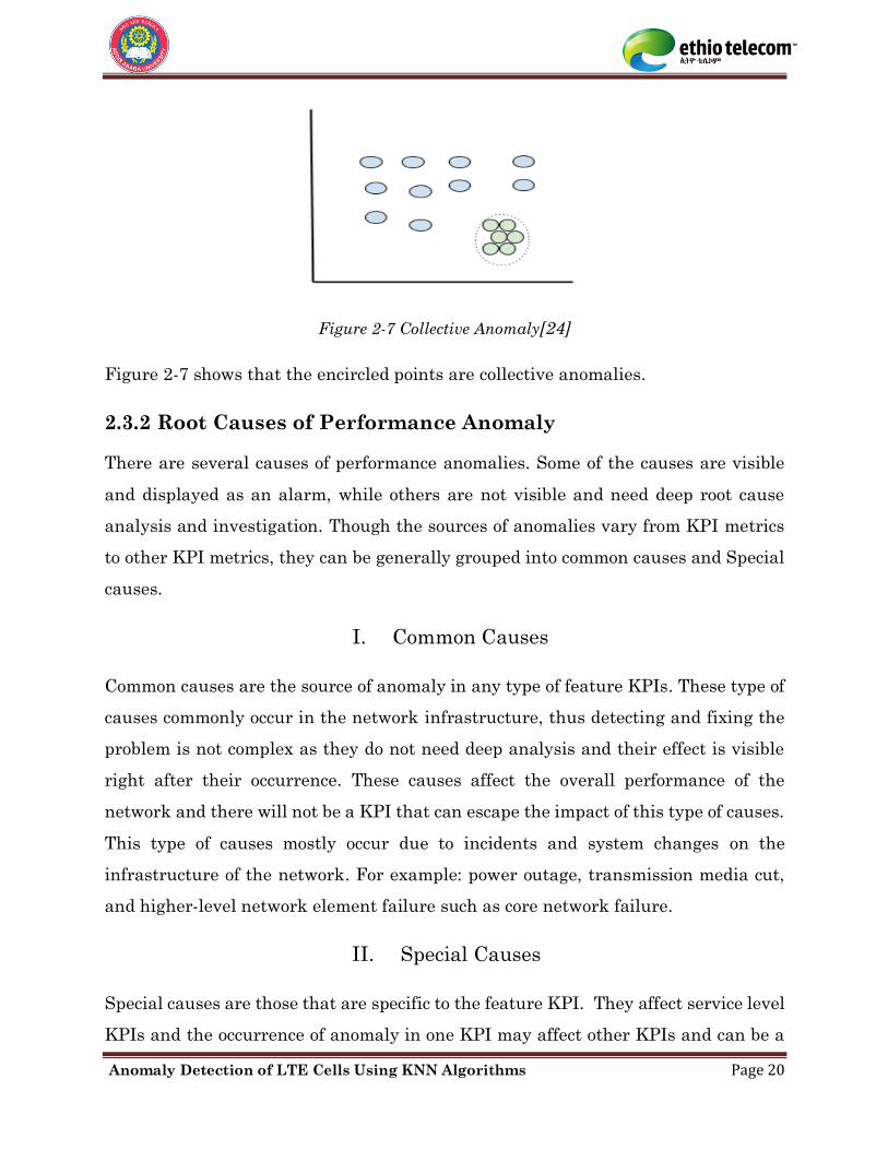
III. Collective Anomalies
If a collection of related data samples is anomalous with respect to other data sets it
is termed as collective anomaly [24]. In collective anomaly the individual data sets
themselves may or may not be anomalies. For example, a cell that is 100% available
but that do not carry enough traffic is a collective anomaly. Cells in the same cluster
showing significant performance drops from the remaining clusters can be considered
as a collective anomaly. A single cell performing in the required range with specified
KPIs, but the combination of the KPIs is not in the required range can also be a
collective anomaly.
Anomaly Detection of LTE Cells Using KNN Algorithms Page 20
Figure 2-7 Collective Anomaly[24]
Figure 2-7 shows that the encircled points are collective anomalies.
2.3.2 Root Causes of Performance Anomaly
There are several causes of performance anomalies. Some of the causes are visible
and displayed as an alarm, while others are not visible and need deep root cause
analysis and investigation. Though the sources of anomalies vary from KPI metrics
to other KPI metrics, they can be generally grouped into common causes and Special
causes.
I. Common Causes
Common causes are the source of anomaly in any type of feature KPIs. These type of
causes commonly occur in the network infrastructure, thus detecting and fixing the
problem is not complex as they do not need deep analysis and their effect is visible
right after their occurrence. These causes affect the overall performance of the
network and there will not be a KPI that can escape the impact of this type of causes.
This type of causes mostly occur due to incidents and system changes on the
infrastructure of the network. For example: power outage, transmission media cut,
and higher-level network element failure such as core network failure.
II. Special Causes
Special causes are those that are specific to the feature KPI. They affect service level
KPIs and the occurrence of anomaly in one KPI may affect other KPIs and can be a
Anomaly Detection of LTE Cells Using KNN Algorithms Page 21
cause for anomaly in another feature KPI too. These kinds of causes include
configuration problem, feature activation or deactivation and parameter changes.
This type of causes usually occur due to human errors for lack of knowledge or
common mistakes. Because performance drops are expected on cells having visible
problem due to common causes, the focus of this thesis work is on anomalies that
occur due to special causes that are not visible and need deep analysis.
Anomaly Detection of LTE Cells Using KNN Algorithms Page 22
3 Anomaly Detection Methods
Authors Erich Schubert and Arthur Zimek defined anomaly detection as “the
identification of rare items, events or observations which raise suspicions by differing
significantly from majority of the data’’. In [3] anomaly detection is defined as the
identification of data points, items, observations or events that do not conform to the
expected pattern of a given group. In this paper anomaly detection is a process of
automatically detecting worst performance cells in specific metrics in a specified time.
3.1 Classification of Anomaly Detection Methods
There are several anomaly detections types. Anomaly detection mechanisms can be
classified considering the following main aspects [25][26].
▪ Nature of input data
▪ Availability of supervision
▪ Type of output
▪ Type of anomaly
▪ Input data set distribution
3.1.1 Nature of Input Data
According to the nature of input data anomaly detection mechanisms can be classified
as univariate and multivariate anomaly detection techniques. The input data sets
can be of numeric, image, text or any other type.
Univariate anomaly detection is a process of detecting anomalies taking a single
variable as an input. The single variable may have several dimensions. For example,
in LTE network service drop rate anomaly detection, the service drop rate may have
day, hour and cell as dimensions, but the target is to find the anomaly value in service
drop rate which is a single variable. In multivariate anomaly detection the detection
of anomalies is from among or a combination of several variables taken as an input.
For example, in LTE network anomaly detection from a cell with KPI metric of service
drop rate and E-RAB setup success rate at the same time is multivariate anomaly

Anomaly Detection of LTE Cells Using KNN Algorithms Page 23
detection. A combination of normal values of univariate anomaly detection for
multiple variables may also create anomaly combination.
Anomaly detection mechanisms based on nature of input data and relationship
among data instances can also be classified as temporal, spatial and spatio-temporal.
In this thesis temporal and spatial anomaly detection are discussed to find the time
of anomaly occurrence and the cell with anomaly performance in a specified metrics.
3.1.2 Outputs of Anomaly Detection
The anomaly detection results of different models are not all the same. Anomaly
results can be either a label (anomaly/not anomaly) or score based. Score based
anomaly results show the degree of abnormality of a sample. For the labeling type
anomaly detection supervised machine learning algorithms with two class
classification are preferred but for the score-based results unsupervised machine
learning, that are based on rank, order or percentile are preferred.
3.1.3 Distribution of Input Data Sets
According to the distribution of input data sets anomaly detection mechanisms are
classified as parametric and nonparametric. Parametric anomaly detection is applied
for anomaly detection of a data with defined probability distribution (normal, poison,
exponential...). With this type of anomaly detection, the anomaly values are those
that are less probable to occur. If p (data sample) < ε, the sample is classified as an
anomaly otherwise it is classified as normal value. Such kind of detection algorithms
are suitable for data labeling type of detection and are not good for detection with
anomaly score [9]. Nonparametric anomaly detection is applied for data set types that
do not rely on data belonging to any parametric family of probability distributions.
Nonparametric distribution do not mean that the data sets are without distribution
but the parameters of the distribution are unspecified [9].

Anomaly Detection of LTE Cells Using KNN Algorithms Page 24
3.1.4 Availability of Supervision
Anomaly detection can be performed manually via statistical analysis. However, for
better accuracy and automation machine learning can be applied. In machine
learning the system is trained with the data sets behavior. According to the
availability of supervision of data labels in the detection process anomaly detection
algorithms are classified as supervised, semi-supervised and unsupervised anomaly
detection.
I. Supervised Anomaly Detection
According to [9][27] a supervised machine learning algorithm is one that relies on
labeled input data to learn a function that produces an appropriate output when given
new unlabeled data. In supervised machine learning a labeled data for normal and
anomaly class is available and the model is trained. The challenge of supervised
anomaly detection is that the proportion of normal to anomaly samples is high and
needs over sampling. KNN classification, regression, support vector machine and
decision trees are the most common supervised anomaly detection algorithms.
II. Semi Supervised Anomaly Detection
According to [9][27] semi supervised anomaly detection is used for a data set with a
known class label for normal data values. The model is trained for a single class and
data samples out of the class are detected as anomalies. When training and testing
data sets are selected for cross validation the combined data set is modeled using
unsupervised anomaly detection. The main problem with this type of detection is that
unseen but legitimate normal values can be classified as anomaly and false negatives
can be generated.
III. Unsupervised Anomaly Detection
According to [9][27] unsupervised anomaly detection algorithms are applied for data
sets that do not have defined class labels. Thus, this model does not need training
Anomaly Detection of LTE Cells Using KNN Algorithms Page 25
and learn the behavior of the data sets by themselves. The unsupervised models
assume the proportion of normal to anomaly values is high. The problem with these
models is that they can detect many small clusters that are not necessarily anomaly.
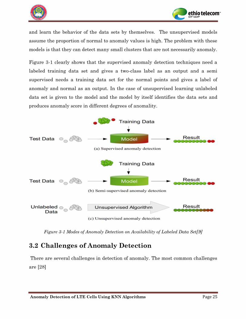
Figure 3-1 clearly shows that the supervised anomaly detection techniques need a
labeled training data set and gives a two-class label as an output and a semi
supervised needs a training data set for the normal points and gives a label of
anomaly and normal as an output. In the case of unsupervised learning unlabeled
data set is given to the model and the model by itself identifies the data sets and
produces anomaly score in different degrees of anomality.
Figure 3-1 Modes of Anomaly Detection on Availability of Labeled Data Set[9]
3.2 Challenges of Anomaly Detection
There are several challenges in detection of anomaly. The most common challenges
are [28]
Anomaly Detection of LTE Cells Using KNN Algorithms Page 26
▪ Defining the normal behavior baseline that usually requires domain expertise.
The fact that normal behavior evolves over time is also a challenge for setting
a baseline.
▪ Availability of labelled data for training and validation
▪ The boundary line between normal and anomaly behavior is not precise
▪ Notion of anomaly depends on context
3.3 Application Areas of Anomaly Detection
Anomaly detection is applicable in several fields of study and operational
activities[9]. Some of the areas are,
▪ Performance monitoring
▪ Fraud detection
▪ Healthcare systems
▪ Fault management
▪ Intrusion detection
Anomaly Detection of LTE Cells Using KNN Algorithms Page 27
4 Anomaly Detection in Addis Ababa LTE KPIs
Ever since LTE network is installed in Addis Ababa in 2015 [29] and the service
became on air ethio telecom is working hard to deliver enhanced service quality to its
customers. LTE KPI monitoring is the systematic process of measuring, analyzing
and using information to track network performance towards reaching the KPI
requirements[17]. KPI monitoring is done to bring cells to a fixed and required
performance value in all KPI metrics[30]. For monitoring purpose, the requirement
for all LTE KPIs is set between ethio telecom and Huawei Tech.co.Ltd. Some of the
LTE KPI requirements set are listed in Table 3. KPI monitoring is not a one-step
task, but a process consisting of measuring KPI values, detecting performance drops,
analyzing and fixing obtained problems.
Table 4-1 Sample KPI Requirement Range in ethio telecom
NO KPI metrics name Required value range
1 RRC setup success rate ≥ 98.5%
2 ERAB setup success rate ≥ 99%
3 Service drop rate ≤ 1%
4 LTE HO success rate ≥ 98%
5 UE context setup success rate ≥ 99%
6 Cell availability ≥ 99%
7 Attach time ≤ 800ms
8 CSFB duration ≤ 5S
9 Call setup success rate ≥ 98%
Anomaly Detection of LTE Cells Using KNN Algorithms Page 28
4.1 LTE KPI Measurement
William Edwards Deming (1900-1993) an American statistician professor and author
quoted “if you can not measure it, you can not manage it”. According to Edwards
performance measurement is the key to deliver quality of service. Performance
measurement is done with defined metrics called key performance indicators (KPI).
KPI measurement is not a one-step task, it is a continuous process that is performed
24X7X365.
LTE KPI measurement is continuously done, and the measurement values are stored
in a database called performance recording system for next action. The measured
values are calculated with a predefined configured logical formula from measured
counter values. Some KPIs that cannot be measured and calculated with defined
formulas from counters such as latency are measured via drive test. KPI
measurement values are calculated from defined and standard formulas. There are
two types of formulas in KPI measurement called physical and logical formulas
[16][19].
I. Physical Formula
In physical formula, KPI value is expressed in terms of the details of counter values.
For example:
RRC Connection Success Counter Setup Success Rate =
Connection Success Counter + RRC Connection Failure CounterRRC
RRC (4-1)
II. Logical Formula
In logical formula, KPI formula is expressed in terms of other KPIs.
For example:
of Successfull ERAB Esatblishments Success Rate =
of Received ERAB Establishment Attempts
NumberERAB Establishment
Number (4-2)
Measured KPIs can be expressed in terms of mean, ratio, cumulative or
combined[18][19].
Anomaly Detection of LTE Cells Using KNN Algorithms Page 29
▪ Mean reflects a mean measurement value based on several sample results. For
For example: average throughput, average traffic
▪ Ratio reflects the percentage of a specific case occurrence to all the cases. For
For example: RRC setup success rate, service drop rate (SDR)
▪ Cumulative reflects a cumulative measurement which is always increasing.
For example: counters, total traffic volume
Percentage, second, erlang and Kbits/sec are some of the units of KPI measurement.
The values that we get from the formulas are the KPI values that are recorded in
PRS. In LTE network the performance measurement takes place in cell level, site
level and overall in the evolved packet core side. For better network management and
effective network QoS monitoring, measurement is mostly done on cell level bases. In
ethio telecom monitoring is done on weekly time intervals by taking daily busy hour
data for analysis as it is practically difficult to manually monitor performance of cells
on daily and hourly time intervals.
4.2 LTE Worst Performing Cells Selection & Analysis
KPI analysis is a process of filtering and identifying cells that do not meet the KPI
requirement, selection of worst performing cells and identification of fault root
causes. In ethio telecom educated guess type of analysis is done manually to select
worst performing cells by considering only the current measured KPI values. In the
case of root cause analysis there are measured counters and alarms that support the
analysis process in the system. Such activities are mostly done with employees that
have higher experience (experts) in the area. The most important part of LTE KPI
analysis is worst performing cell selection process.
Considering the threshold values shown in Table 4-1, ethio telecom uses two scale
(above and below the requirement) fixed threshold in all KPIs metrics and all the
time for network monitoring. This fixed threshold does not vary with the dynamic
nature of LTE network performance. During performance comparison of cells with
the requirement with defined metrics several cells do not meet the target values even
Anomaly Detection of LTE Cells Using KNN Algorithms Page 30
when the average performance value of the cell with respect to the defined metrics is
greater than the minimum required KPI value. In the current KPI monitoring process
of Addis Ababa LTE network, no effort is done to farther improve the performance
value if the value is within the required range. For example, the required value range
for RRC setup success rate is ≥ 98.5%, if the measured value of the metrics is 98.5 the
analyst and radio expert will not try to improve it to 100% even when there is a
possibility. It is because ethio telecom is using fixed threshold and the recorded value
has meet the requirement.
For cells that are with KPI values less than the requirement a corrective action to
recover or compensate the performance drop needs to be taken. Because the
performance recovery or compensation can not be done for all the cells at the same
time prioritization of the cells for corrective actions is important. Thus, the cells with
lower performance value are given priority after observing their current performance
value. This method is not efficient as it is not able to check back the performance
history of the cells in the specified metrics.
After having the measurement detail investigation of all the cells is done and cells
with the required performance range and those with a performance drop are
manually filtered. The manual filtering mechanism more focuses on current values
and lacks accuracy to include the history performance of each cell. However, in
machine learning based anomaly detection, worst cell selection can consider both the
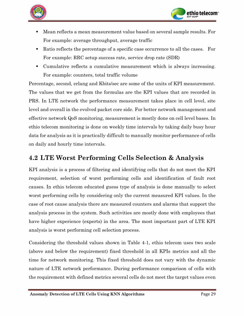
current values and the performance history as shown in Figure 4-1.
Figure 4-1 Manual Worst Cell Selection vs Automatic Anomaly Detection

Anomaly Detection of LTE Cells Using KNN Algorithms Page 31
In Figure 4-1 it is clearly seen that in manual worst cell selection of a single KPI
metrics column wise value comparison is done for daily data and is difficult to
consider the performance history, but in automated anomaly detection worst cell
selection, considering the current value as well as the history performance is possible.
The manual anomaly detection becomes more complex for detecting anomaly cells
with multiple KPI metrics simultaneously.
There are several KPIs for each cell and manual worst performing cell selection is
time consuming and sometimes difficult to do it on time. When the selected worst
performing cell list are prepared as a report to different zones of Addis Ababa there
is a problem of not accepting the report. Complaints on reports to different
departments and zones brings a question of credibility. These less credible reports
are observed to lead for wrong decisions that do not bring a performance improvement
and sometimes for worse performance. The manual worst performing cells selection
is routine and tiresome for employees and this creates employee dissatisfaction in the
work and lets employees to work extra hours from the normal working hours. For this
reason, ethio telecom pays additional payment as an incentive for employees involved
in the work.
Anomaly Detection of LTE Cells Using KNN Algorithms Page 32
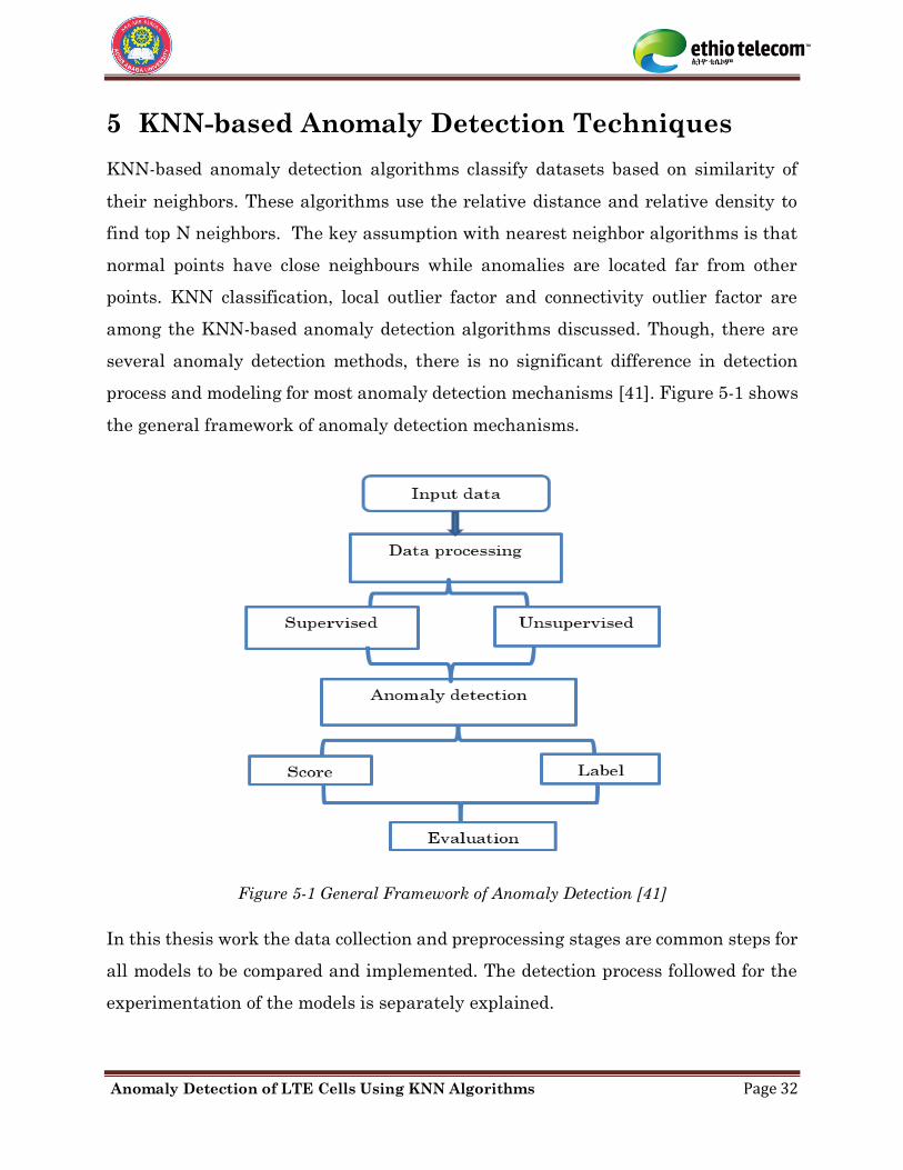
5 KNN-based Anomaly Detection Techniques
KNN-based anomaly detection algorithms classify datasets based on similarity of
their neighbors. These algorithms use the relative distance and relative density to
find top N neighbors. The key assumption with nearest neighbor algorithms is that
normal points have close neighbours while anomalies are located far from other
points. KNN classification, local outlier factor and connectivity outlier factor are
among the KNN-based anomaly detection algorithms discussed. Though, there are
several anomaly detection methods, there is no significant difference in detection
process and modeling for most anomaly detection mechanisms [41]. Figure 5-1 shows
the general framework of anomaly detection mechanisms.
Figure 5-1 General Framework of Anomaly Detection [41]
In this thesis work the data collection and preprocessing stages are common steps for
all models to be compared and implemented. The detection process followed for the
experimentation of the models is separately explained.

Anomaly Detection of LTE Cells Using KNN Algorithms Page 33
5.1 Assumptions
Though measurement errors are expected, it is assumed that the errors made by the
measuring system is negligible. Thus, recorded performance drops are assumed to be
due to configuration change, parameter change and unexpected incidents. If critical
or major alarm is not observed in the specified time, performance drop of cells is
expected to occur due to configuration/ reconfiguration problems and not due to
common anomaly causes.
5.2 KNN Classification System Model
KNN classification is a supervised machine learning model used to classify data sets
in to two labels based on the label of majority of its neighbors. The KNN algorithm
assumes that similar things exist in proximity. The quote “birds of the same feather
flock together” better explains the KNN classification. It is a nonparametric
classification method that classifies data sets based on learning from training data
sets. The process model of KNN classification implemented in this thesis work is
shown in Figure 5-2.
Figure 5-2 KNN Classification Process Model
Anomaly Detection of LTE Cells Using KNN Algorithms Page 34
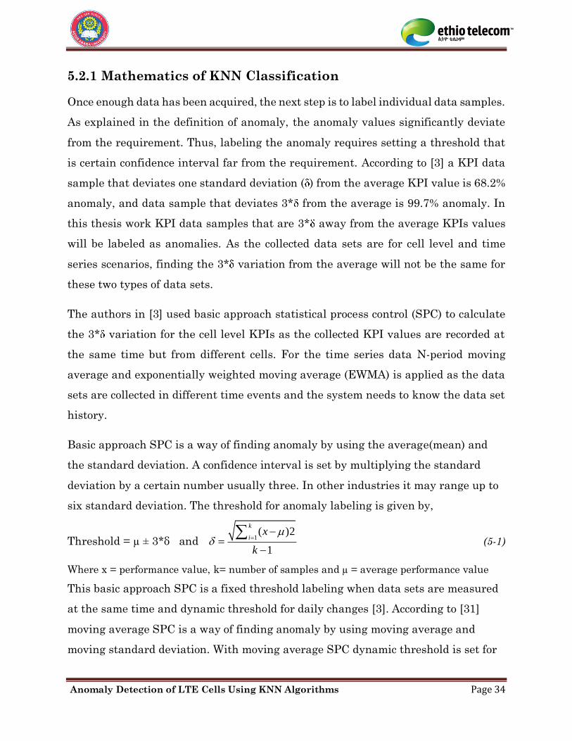
5.2.1 Mathematics of KNN Classification
Once enough data has been acquired, the next step is to label individual data samples.
As explained in the definition of anomaly, the anomaly values significantly deviate
from the requirement. Thus, labeling the anomaly requires setting a threshold that
is certain confidence interval far from the requirement. According to [3] a KPI data
sample that deviates one standard deviation ( ) from the average KPI value is 68.2%
anomaly, and data sample that deviates 3* from the average is 99.7% anomaly. In
this thesis work KPI data samples that are 3* away from the average KPIs values
will be labeled as anomalies. As the collected data sets are for cell level and time
series scenarios, finding the 3* variation from the average will not be the same for
these two types of data sets.
The authors in [3] used basic approach statistical process control (SPC) to calculate
the 3* variation for the cell level KPIs as the collected KPI values are recorded at
the same time but from different cells. For the time series data N-period moving
average and exponentially weighted moving average (EWMA) is applied as the data
sets are collected in different time events and the system needs to know the data set
history.
Basic approach SPC is a way of finding anomaly by using the average(mean) and
the standard deviation. A confidence interval is set by multiplying the standard
deviation by a certain number usually three. In other industries it may range up to
six standard deviation. The threshold for anomaly labeling is given by,
Threshold = µ ± 3*δ and 1( )2
1
k
ix
k
=
−=
−
(5-1)
Where x = performance value, k= number of samples and µ = average performance value
This basic approach SPC is a fixed threshold labeling when data sets are measured
at the same time and dynamic threshold for daily changes [3]. According to [31]
moving average SPC is a way of finding anomaly by using moving average and
moving standard deviation. With moving average SPC dynamic threshold is set for
Anomaly Detection of LTE Cells Using KNN Algorithms Page 35
anomaly labeling and samples are given equal weight regardless of the time
occurrence. This type of labeling is more comfortable for time series data set
labeling. The threshold for anomaly labeling is given by,
3*Threshold y n= and,
2
1
( )
1
K
K m
yi y
nm
− +
−
=−
where M is window size (5-2)
The moving average also called M-point moving average, is calculated in fixed points
of window size.
EWMA based SPC is a way finding anomalies by using moving average and moving
standard deviation. With EWMA samples are with different weights and the weight
exponentially increases from the oldest data sample to the recent data samples. The
threshold for anomaly labeling is given by,
3Threshold EWMAt EWMAt= where, (1 ) 1EWMAt Yt EWMAt = + − − (5-3)
where, λ = waiting factor
The EWMA standard deviation is calculated in relation to the moving average
standard deviation by,
( 2)(2 )
EWMA n
= −
(5-4)
The next step in KNN classification is setting the value of K. According to [32] there
is no standard mechanism to determine optimal value of K, however K should not be
too small and too large, usually recommended to be odd, less or equal to the squared
root of number of training data samples.
There are several mechanisms to find distance of a data sample to all other data
samples. According to [33] Euclidian distance is more suitable for finding the distance
between two KPI data set points. The Euclidian distance is given by the formula,
1
( , ) ( )2n
i
D X Y xi yi=
= − (5-5)

Anomaly Detection of LTE Cells Using KNN Algorithms Page 36
After sorting the calculated Euclidian distance top K nearest data samples are
selected as KNN. Authors in [32] explained that all samples in the KNN do not have
equal contribution in labeling a data sample. The first neighbor has higher weight and
the kth neighbor is with the least weight. The next step in KNN classification is to find
the total number of neighbors N1 and N2 in each class and determine the sum of their
inverted distances with formulas, [32]
1( 1)
1
1( )1
N
i ci
S xN
= ==
and
1( 2)
1
2( ) , 1,2,3.....2
N
i ci
S x i KN
= == =
(5-6)
Finally find probability of a point X belongs to each class is calculated by the formulas
below.
1( )
( 1| )1( ) 2( )
S xP c X
S x S x= =
+ and
2( )( 2 | )
1( ) 2( )
S xP c X
S x S x= =
+ (5-7)
Then, data is in class 1 if ( 1| )P c X= > 0.5 and in class 2 if ( 2 | )P c X= > 0.5.
Prepared and labeled training data sets may not be enough for the model to enable
new data set classification and may lead to model underfitting. According to [45] a
technique called N-fold cross validation can be used as a remedy by removing a part
of the training data and using it to get predictions from the model trained on rest of
the data. This mechanism is called holdout. In N-fold cross validation, the data is
divided into n subsets. Now the holdout method is repeated N times, such that each
time, one of the N subsets is used as the test set/ validation set and the other N-1
subsets are put together to form a training set. Higher value of N leads to model
overfitting and lower value of N leads to model underfitting. Thus, optimal value of
N should be selected to give more accurate prediction result. Though, there is no clear
selection criteria of N, the mostly applied 5 to 10-fold cross validation [46] is
implemented in this thesis work.
Anomaly Detection of LTE Cells Using KNN Algorithms Page 37
5.3 Density-based Local Outlier Factor
As discussed in [34] by comparing the local density of an object to the local densities
of its neighbors, one can identify regions of similar density and points that have a
substantially lower density than their neighbors. In 2000 authors called Markus M.
Breunig, Hans-Peter Kriegel and Jörg Sander identified a mechanism of finding
anomalous data points by measuring the local deviation of a given data point with
respect to its neighbors. These authors named this algorithm LOF.
LOF is unsupervised machine learning anomaly detection model that investigates
the density of an object and its neighbors. According to [22] an object is identified as
an anomaly if its density is relatively much lower than that of its neighbors. The basic
idea that differentiates LOF from the classification models is that being anomaly is
not a binary property, instead, to each object an outlier factor is assigned, which is the
degree the object is being outlying [34]. The challenge with ordinary local outlier factor
is finding K-nearest neighbors in the presence of duplicate data samples. Several LTE
KPIs are with the same performance values and these duplicate values are confusing
and complex for the LOF algorithm to determine the fixed K neighbors for each data
sample. Thus, it is recommended that local outlier factor given duplicates should be
implemented for LTE cells anomaly detection [35].
5.3.1 System Model of Local Outlier Factor
Unsupervised learning algorithms do not need training data sets and the algorithms
by themselves learn the data set behavior. As LOF is unsupervised machine learning
algorithm, preparation of training data is not important for experimentation, but the
labeled data sets are used for performance evaluation. As COF is a modified version
of LOF there is no difference in the general process model. The process model for LOF
and COF in this thesis work is shown in Figure 5-3.
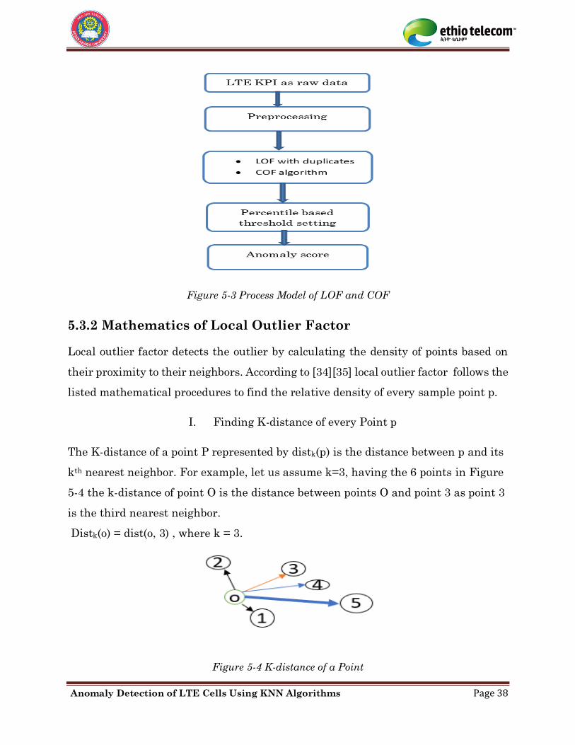
Anomaly Detection of LTE Cells Using KNN Algorithms Page 38
Figure 5-3 Process Model of LOF and COF
5.3.2 Mathematics of Local Outlier Factor
Local outlier factor detects the outlier by calculating the density of points based on
their proximity to their neighbors. According to [34][35] local outlier factor follows the
listed mathematical procedures to find the relative density of every sample point p.
I. Finding K-distance of every Point p
The K-distance of a point P represented by distk(p) is the distance between p and its
kth nearest neighbor. For example, let us assume k=3, having the 6 points in Figure
5-4 the k-distance of point O is the distance between points O and point 3 as point 3
is the third nearest neighbor.
Distk(o) = dist(o, 3) , where k = 3.
Figure 5-4 K-distance of a Point
Anomaly Detection of LTE Cells Using KNN Algorithms Page 39
II. K-distance Neighborhood of P
k-distance neighborhood of p represented by Nk(p) is the number of objects (a set of
objects) that are a distance D less or equal to distk(p) away from point p. The k-
distance neighborhood of p contains set of points whose distance from p is not greater
than the k-distance. Nk (p) could be bigger than K since multiple objects may have
an identical distance to point P.
( ) ( ) ( ) ,| ’ ’ , ’ Nk p p p in D dist p p distk p= (5-8)
III. Reachability Distance of Point P
The reachability distance represented by reachdistk (P←P’) is the maximum of the
reachability distance of point p and reachability distance of p’s k-nearest neighbors.
( ) ( ) ( ) ’ , , ’ k kreachdist p p max dist p dist p p = (5-9)
LOF uses reachability distance to find nearest neighbors unlike Euclidean distance
in KNN classification. Finding reachability distance reduces the statistical
fluctuation of finding distances dist(p,p’).
IV. Local Reachability Density of Point p.
Local reachability density of P represented by lrdk(P) is the ratio of k-distance
neighborhood of p to sum of reachability distance from P’ to P. it can also be defined
as the inverse of the average reachability distance.
' ( )
|| ( ) ||( )
( ' )P Nk P
Nk Plrdk P
reachdistk P P
=
(5-10)
V. Local Outlier Factor of Point p.
Local outlier factor represented by LOFk(p) is the average of the ratio of local
reachability of p and those of p’s k-nearest neighbors and is given by,
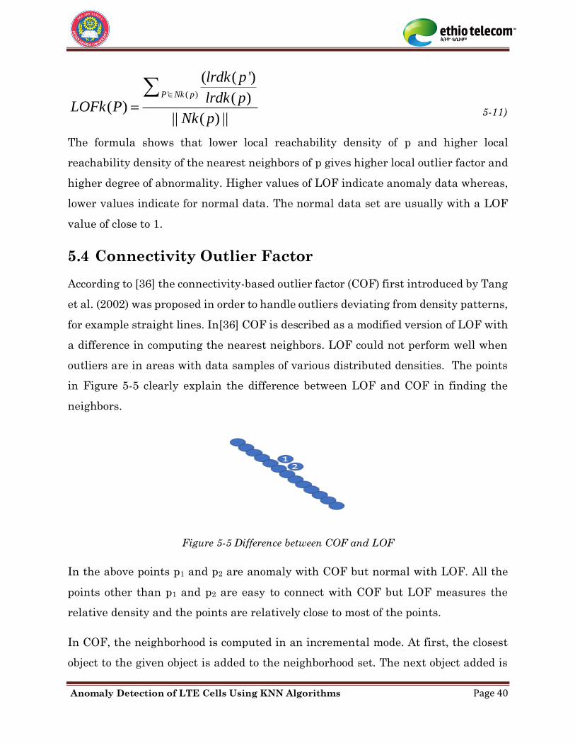
Anomaly Detection of LTE Cells Using KNN Algorithms Page 40
' ( )
( ( ')
( )( )
|| ( ) ||
P Nk p
lrdk p
lrdk pLOFk P
Nk p
=
5-11)
The formula shows that lower local reachability density of p and higher local
reachability density of the nearest neighbors of p gives higher local outlier factor and
higher degree of abnormality. Higher values of LOF indicate anomaly data whereas,
lower values indicate for normal data. The normal data set are usually with a LOF
value of close to 1.
5.4 Connectivity Outlier Factor
According to [36] the connectivity-based outlier factor (COF) first introduced by Tang
et al. (2002) was proposed in order to handle outliers deviating from density patterns,
for example straight lines. In[36] COF is described as a modified version of LOF with
a difference in computing the nearest neighbors. LOF could not perform well when
outliers are in areas with data samples of various distributed densities. The points
in Figure 5-5 clearly explain the difference between LOF and COF in finding the
neighbors.
Figure 5-5 Difference between COF and LOF
In the above points p1 and p2 are anomaly with COF but normal with LOF. All the
points other than p1 and p2 are easy to connect with COF but LOF measures the
relative density and the points are relatively close to most of the points.
In COF, the neighborhood is computed in an incremental mode. At first, the closest
object to the given object is added to the neighborhood set. The next object added is

Anomaly Detection of LTE Cells Using KNN Algorithms Page 41
the one with its distance to the existing neighborhood to be minimum among all
remaining objects. The distance between an object and a set of objects is defined as
the minimum distance between the given object and any object belonging to the given
set. In this fashion the neighborhood continues until it reaches size K.
5.4.1 Mathematics of Connectivity Outlier Factor
Connectivity outlier factor detects the outlier by calculating the density of points based
on their proximity to their neighbors considering least cost and shortest path.
According to [36][37] the mathematical procedures in calculating the values of COF
are,
I. Set of k-nearest Neighbors of Point p
The set of k-nearest neighbors represented by Nk(P) is a list of all nearest neighbors
to point p.
( ) 1, 5 3 , . KN P p p p Pk= (5-12)
II. Set-based Nearest Trial
Set-based nearest trial is a set of all possible combination of nearest paths. Set based
nearest trail of data point P is set of points , such that for all 1 ≤ i ≤ k −1, pi+1 is the
nearest neighbor point of set {p1,···,pi} in set {pi+1,···,pk}. where i is the index of the
nearest neighbors. where i = 1,2,3…. k.
III. Set-based Nearest Path
Set-based nearest path of point p is the set of neighbor points in the order of their
proximity to point p. The set based nearest path can be given in set-based sequence
of edges as,
1 5 7 , , ,.....
KSBN edges e e e e= (5-13)
IV. Cost of Set-based Nearest Trial
Anomaly Detection of LTE Cells Using KNN Algorithms Page 42
The cost of set-based nearest trial is a set of distance between two nearest neighbors
in the set of Nk(P). for example, for k=5 the set can be given as SBN cost =
{5,4,3,2,1,1}.
V. Average Chaining Distance of Point p
Average chaining distance can be expressed as the average of the weighted
distances in the cost description of the SBN-trail. The average chaining distance is
given by,
1
2( 1 1)( ) ( ) * ( )
( 1)
K
i
kac distNk p p P dist ei
k k=
+ −− =
+ (5-14)
where dist(ei) is the sum of cost to reach all nearest neighbors.
VI. Connectivity Outlier Factor
COF is the ratio of the average chaining distance from data record p to Nk(p) and the
averaged average chaining distances at the record’s neighborhood. The COF value is
calculated by the formula,
0 ( )
( ) ( )( )
( ) ( )Nk p
ac distNk p p PCOF p
ac distNk o o o
k
− =
− (5-15)
The calculated value of COF is finally the anomaly score of the model.
5.5 Performance Evaluation Mechanisms of Anomaly Detection
To compare and get the most accurate anomaly detection model requires performance
evaluation of the models. The outputs of the training and learning of the algorithm
need to be assessed and analyzed carefully and the result needs to be interpreted to
evaluate the algorithm [33][38]. The performance of anomaly detection algorithms is
usually measured by their detection accuracy. But accuracy alone is not enough
metric for evaluation. Thus, standard measures for evaluating anomaly detection
performance are [38][39].
Anomaly Detection of LTE Cells Using KNN Algorithms Page 43
▪ Recall (true positive rate) is the ratio between the number of correctly
detected anomalies and the total number of anomalies and is given by.
posetiveRe
posetive + False negative
Truecall
True= (5-16)
▪ Precision (false positive rate) is the ratio of the number of data records from
the normal class that are misclassified as anomalies and the total number
of data records in normal class and is given by,
posetivePrecision =
posetive + False posetive
True
True (5-17)
▪ ROC curve is a trade-off between recall and precision rate. It tells how much
a model is capable of distinguishing between classes. The ROC curve is
usually plotted with TPR on y-axis and FPR on the x-axis.
▪ Area under the ROC curve (AUC) is the area under the graphical plot of the
true positive rate against the false positive rate, where the true (false)
positive rate represents the proportion of detected anomalies among the top
n potential anomalies. Higher AUC values indicate better prediction
capability of models and better detection accuracy.
As the anomaly detection model has to catch as many outliers as possible and is
expected to not mislabel normal objects as anomalies, recall is more important than
accuracy[40]. According to [38] for high proportion of one class to the other precision
recall curves are preferred among the available measures.

Anomaly Detection of LTE Cells Using KNN Algorithms Page 44
6 Experimentation and Result Analysis
6.1 Data Collection and Preprocessing
LTE KPI measurements are collected from performance recording systems. According
to [42] performance monitoring is better done when the KPI spacing is on hourly and
daily granularity. Thus, for experimentation of this thesis work ten days (04/01/2019
to 04/10/2019) daily RRC setup success rate, E-RAB setup success rate and service
drop rate of all LTE cells in Addis Ababa is collected for the cell level detection
scenario and one month hourly RRC setup success rate, E-RAB setup success rate
and service drop rate of all LTE cells is collected for April 2019.
All the collected raw data is not meaningful, instead, it contains several missed and
inconsistent values. Thus, such kind of raw data need to be filtered out and the
remaining data should be considered for the anomaly detection input. It is expected
that if there is an alarm, performance will significantly drop. Thus, cells with critical
and major alarm are also filtered out and not included in the experimentation as it is
assumed that the drop is due to the alarm. Other activities such as data set labeling,
distribution fitting and model training activities are performed in the preprocessing
stage.
6.1.1 Distribution Fitting
Knowing the distribution from which we are going to assume the data set was
generated from is not easy and fitting the data to the chosen distribution to obtain the
best estimate effectively need to be done. Most KPIs are given in bounded percentages
between 0% and 100%. Thus, the distribution type of the KPIs is almost the same.
To make sure the distribution fitting estimation generalizes well to the population
and not just the sample data fitting of three months RRC setup success rate and
service drop rate to represent right and left skewed data samples is done and the
result is as shown in Figures 6-1 and 6-2.
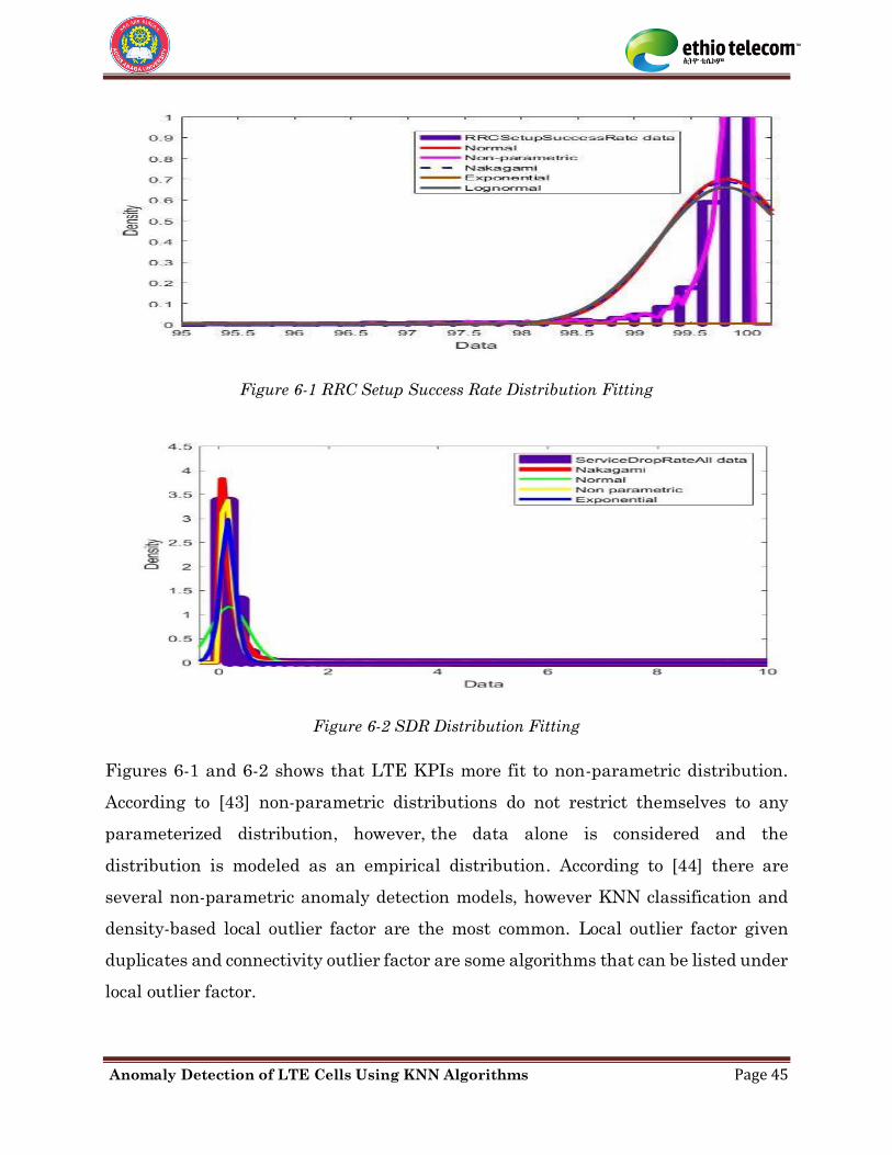
Anomaly Detection of LTE Cells Using KNN Algorithms Page 45
Figure 6-1 RRC Setup Success Rate Distribution Fitting
Figure 6-2 SDR Distribution Fitting
Figures 6-1 and 6-2 shows that LTE KPIs more fit to non-parametric distribution.
According to [43] non-parametric distributions do not restrict themselves to any
parameterized distribution, however, the data alone is considered and the
distribution is modeled as an empirical distribution. According to [44] there are
several non-parametric anomaly detection models, however KNN classification and
density-based local outlier factor are the most common. Local outlier factor given
duplicates and connectivity outlier factor are some algorithms that can be listed under
local outlier factor.
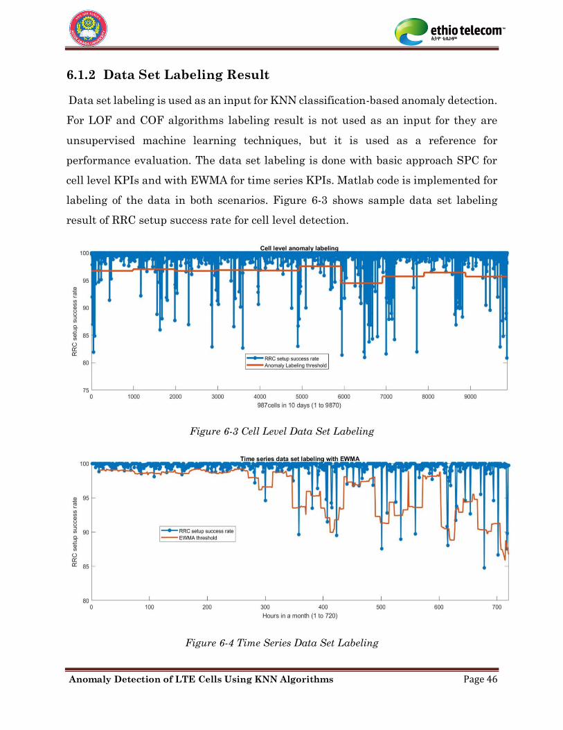
Anomaly Detection of LTE Cells Using KNN Algorithms Page 46
6.1.2 Data Set Labeling Result
Data set labeling is used as an input for KNN classification-based anomaly detection.
For LOF and COF algorithms labeling result is not used as an input for they are
unsupervised machine learning techniques, but it is used as a reference for
performance evaluation. The data set labeling is done with basic approach SPC for
cell level KPIs and with EWMA for time series KPIs. Matlab code is implemented for
labeling of the data in both scenarios. Figure 6-3 shows sample data set labeling
result of RRC setup success rate for cell level detection.
Figure 6-3 Cell Level Data Set Labeling
Figure 6-4 Time Series Data Set Labeling
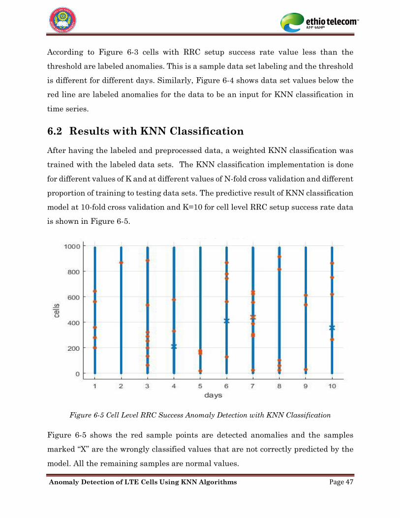
Anomaly Detection of LTE Cells Using KNN Algorithms Page 47
According to Figure 6-3 cells with RRC setup success rate value less than the
threshold are labeled anomalies. This is a sample data set labeling and the threshold
is different for different days. Similarly, Figure 6-4 shows data set values below the
red line are labeled anomalies for the data to be an input for KNN classification in
time series.
6.2 Results with KNN Classification
After having the labeled and preprocessed data, a weighted KNN classification was
trained with the labeled data sets. The KNN classification implementation is done
for different values of K and at different values of N-fold cross validation and different
proportion of training to testing data sets. The predictive result of KNN classification
model at 10-fold cross validation and K=10 for cell level RRC setup success rate data
is shown in Figure 6-5.
Figure 6-5 Cell Level RRC Success Anomaly Detection with KNN Classification
Figure 6-5 shows the red sample points are detected anomalies and the samples
marked “X” are the wrongly classified values that are not correctly predicted by the
model. All the remaining samples are normal values.

Anomaly Detection of LTE Cells Using KNN Algorithms Page 48
The confusion matrix of the KNN classification for trained data sets of cell level
anomaly detection showed a TPR of 93% and a true negative rate of > 99% as shown
in Table 4.
Table 6-1 Confusion Matrix for Cell Level KNN Classification
Table 6-2 Confusion Matrix of Time Series KNN Classification
Similarly, the confusion matrix for time series anomaly detection showed a TPR of
88% and a TNR of >99% as shown in Table 5. The higher value of TNR in both
scenarios is due to the high proportion of normal to anomaly values.
6.3 Results with Local Outlier Factor
Anomaly detection results in local outlier factor are given in terms of anomaly score
and not labels. Values close to 1 are close to the normal value and the higher the
score the more the sample is anomaly. Anomaly score values of the data sets are
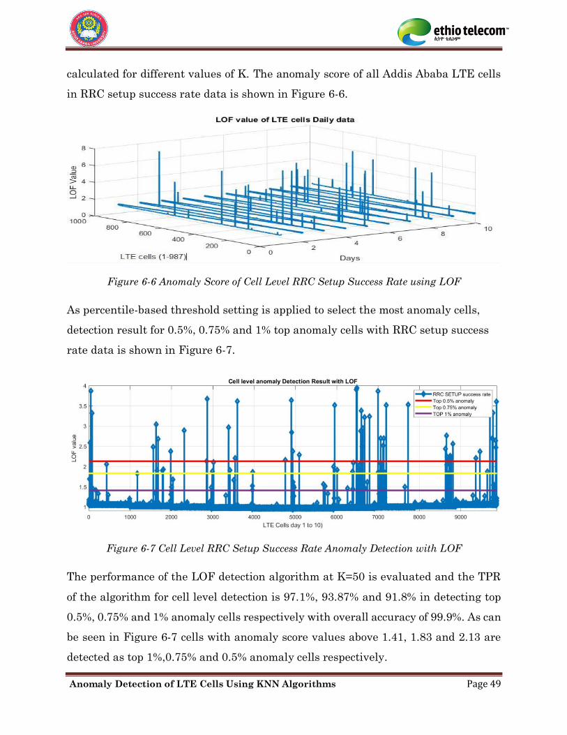
Anomaly Detection of LTE Cells Using KNN Algorithms Page 49
calculated for different values of K. The anomaly score of all Addis Ababa LTE cells
in RRC setup success rate data is shown in Figure 6-6.
Figure 6-6 Anomaly Score of Cell Level RRC Setup Success Rate using LOF
As percentile-based threshold setting is applied to select the most anomaly cells,
detection result for 0.5%, 0.75% and 1% top anomaly cells with RRC setup success
rate data is shown in Figure 6-7.
Figure 6-7 Cell Level RRC Setup Success Rate Anomaly Detection with LOF
The performance of the LOF detection algorithm at K=50 is evaluated and the TPR
of the algorithm for cell level detection is 97.1%, 93.87% and 91.8% in detecting top
0.5%, 0.75% and 1% anomaly cells respectively with overall accuracy of 99.9%. As can
be seen in Figure 6-7 cells with anomaly score values above 1.41, 1.83 and 2.13 are
detected as top 1%,0.75% and 0.5% anomaly cells respectively.
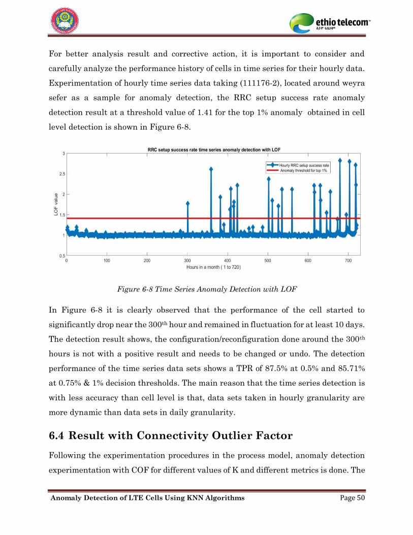
Anomaly Detection of LTE Cells Using KNN Algorithms Page 50
For better analysis result and corrective action, it is important to consider and
carefully analyze the performance history of cells in time series for their hourly data.
Experimentation of hourly time series data taking (111176-2), located around weyra
sefer as a sample for anomaly detection, the RRC setup success rate anomaly
detection result at a threshold value of 1.41 for the top 1% anomaly obtained in cell
level detection is shown in Figure 6-8.
Figure 6-8 Time Series Anomaly Detection with LOF
In Figure 6-8 it is clearly observed that the performance of the cell started to
significantly drop near the 300th hour and remained in fluctuation for at least 10 days.
The detection result shows, the configuration/reconfiguration done around the 300th
hours is not with a positive result and needs to be changed or undo. The detection
performance of the time series data sets shows a TPR of 87.5% at 0.5% and 85.71%
at 0.75% & 1% decision thresholds. The main reason that the time series detection is
with less accuracy than cell level is that, data sets taken in hourly granularity are
more dynamic than data sets in daily granularity.
6.4 Result with Connectivity Outlier Factor
Following the experimentation procedures in the process model, anomaly detection
experimentation with COF for different values of K and different metrics is done. The
Anomaly Detection of LTE Cells Using KNN Algorithms Page 51
anomaly score of all Addis Ababa LTE cells in RRC setup success rate data is shown
in Figure 6-9.
Figure 6-9 Anomaly Score of RRC Setup Success Rate with COF
As percentile-based threshold setting is applied to select the most anomaly cells,
detection result of 0.5%, 0.75% and 1% top anomaly cells with RRC setup success rate
data is shown in Figure 6-10.
Figure 6-10 Cell Level RRC Setup Success Rate Anomaly Detection with COF
The decision thresholds are 1.19,1.31 and 1.45 for detecting top 1%, 0.75% and 0.5%
anomaly cells respectively. The detection performance of COF at K=50 is evaluated
and the TPR of the algorithm for cell level detection is 97.9%, 95.91% and 93.87% in

Anomaly Detection of LTE Cells Using KNN Algorithms Page 52
detecting 0.5%, 0.75% and 1% top anomaly cells respectively with overall accuracy of
99.9%. The less performance value for high percentage thresholds is, because for
higher percentage thresholds it becomes challenging to separate the normal and
anomaly values as the performance of anomaly cells becomes closer to normal.
Time series anomaly detection is also done for (111176-2) as a sample. The time series
anomaly detection of RRC setup success rate of the cell using COF for the 0.5%
anomaly decision threshold of 1.45 is shown in Figure 6-11.
Figure 6-11 Time Series Anomaly Detection with COF for Hourly RRC Setup Success Rate
For the time series data sets a TPR of 87.5% for 0.5% & 0.75%, and 85.71% for 1% top
anomaly cells in RRC setup success rate is recorded using COF. Figure 6-11 shows
the experimented cell has been with a good RRC setup success rate performance for
the first 350 hours of the month and anomaly performance behaviors are observed
after the 350th hour and remained unfixed for the remaining hours of the month with
fluctuating performance values.
Anomaly detection of SDR cell level data at k=50 using COF is as explained in Figure
6-12. The performance result is 95.91% for detecting 0.5% & 0.75%, and 93.87% for
1% top anomaly cells.
Anomaly Detection of LTE Cells Using KNN Algorithms Page 53
Figure 6-12 Cell Level SDR Anomaly Detection with COF
Anomaly detection experimentation for E-RAB setup success rate is also done
following the same procedures with that of RRC setup success rate & SDR. The
detection result at K=50 is shown in Figure 6-13. The decision thresholds are 1.17,
1.31 and 1.41 for detecting 1%, 0.75% and 0.5% top anomaly cells. The performance
of detecting top 0.5%, 0.75% and 1% anomaly cells is 96%, 94.74%, 94.11%
respectively.
Figure 6-13 Cell Level E-RAB Setup Anomaly Detection with COF
Anomaly Detection of LTE Cells Using KNN Algorithms Page 54
Performance anomaly in one KPI is the cause for anomaly in several other KPIs. In
this case deep root cause analysis for the performance anomalies needs to be done.
The experimentation with COF is also done for time series anomaly detection.
Figure 6-14 shows the existence of performance anomaly in one or two of KPI metrics
can be a cause for performance anomaly in other KPI metrics.
Figure 6-14 Anomaly Interdependence among Different KPI Metrices
6.5 Performance Comparison and Discussion
Anomaly detection algorithms can be compared in different aspects. The type of
output, complexity and result accuracy are some of the comparison criterions
considered in this thesis work. In this regard LOF and COF that can provide outputs
as anomaly score are better than KNN classification that outputs two-class labels as
Anomaly Detection of LTE Cells Using KNN Algorithms Page 55
the goal of anomaly detection is to select topmost anomaly cells. Regarding
complexity, though KNN classification requires heavy training it is less complex than
LOF & COF, as finding the relative density of sample data sets needs deep
calculation. COF is more complex than LOF in finding cost and shortest path by
calculating SBN trials and SBN edges.
The individual performance evaluation of the algorithms showed that better results
are achieved at K=10 with KNN classification, at K=50 and k=25 with LOF, at K=50
and k=25 with COF for the cell level and time series detection respectively.
Performance comparison of the algorithms at their best performance condition with
respect to their TPR is shown in Figure 6-15.
Figure 6-15 Performance Comparison of KNN-based Anomaly Detection Algorithms
The experimentation result shows that, accuracy of all the algorithms is similar and
no significant difference is observed. As can be clearly seen in Figure 6-15 the TPR of
the specified algorithms is almost the same but the COF seems to have better
detection for a larger percentile range. The Figure shows a decreasing TPR of
detecting anomalies for higher percentile-based thresholds. But for the KNN

Anomaly Detection of LTE Cells Using KNN Algorithms Page 56
classification the TPR is not percentile dependent as it outputs two-class labels. The
time series anomaly detection of the KNN classification remained the same at 5 to
10-fold cross validation.
The high accuracy in TNR for both scenarios is due to high proportion of normal to
anomaly samples, and the lower TPR in time series detection than cell level detection
is due to higher dynamic nature of KPIs in hourly granularity than in daily
granularity. Thus, the more the nature of data samples is dynamic the more it
becomes difficult for the algorithm to predict the output. Detection accuracy also
becomes less when considering higher percentage of anomaly thresholds in LOF and
COF as the performance value of anomaly cells become close to normal and then
difficult for the algorithms to predict.
Anomaly Detection of LTE Cells Using KNN Algorithms Page 57
7 Conclusion and Future Work
7.1 Conclusion
Anomaly detection is one common operational task of mobile operators so that
network problems are timely identified, and corrective actions are taken. The
Ethiopian sole operator, ethio telecom is currently applying manual and subjective
anomaly detection method, which is maintenance time, manpower and then cost
inefficient. To address this problem automatic anomaly cell detection method using
machine learning algorithms has been proposed, implemented and evaluated in this
thesis work. Anomaly cells can be detected by the measured value of different KPI
metrics from network management system. Anomaly cell with respect to one KPI
metrics can be normal when measured with respect to another KPIs. Considering
type of data sets, distribution type of data sets, required type of output and
availability of supervision KNN-based anomaly detection methods are found to be
more suitable for cell anomaly detection of Addis Ababa LTE networks.
KNN classification, LOF and COF algorithms are implemented and compared for cell
level and time series scenarios. Considering type of output and availability of
supervision the KNN classification is less preferable than LOF and COF as it outputs
two-class labels and needs heavy training. Comparison result of anomaly detection
capability of the algorithms shows that three of them are with negligible performance
difference while COF showing slightly better TPR. Though COF is with better
detection capability it is more complex than KNN classification and LOF in finding
the shortest path for connectivity.
7.2 Future Work
In the future this anomaly detection algorithms can be done for detection of anomaly
cells using multivariate KPIs. It can also be done for fault prediction, fault root cause
detection and outage detection. Anomaly detection for other Technologies such as FL
NGN and IP networks can also be part of the future work.
Anomaly Detection of LTE Cells Using KNN Algorithms Page 58
References
[1] T. Tsvetkov, S. Nováczki, H. Sanneck, and G. Carle, “A Configuration
Management Assessment Method for SON Verification,” 11th Int. Symp. Wirel.
Commun. Syst. ISWCS 2014 - Proc., pp. 380–384, 2014.
[2] Vista Solutions, “Self-Optimizing Solution for 2G , 3G and 4G Mobile
Networks.”, 2012.
[3] D. Kakadia, J. Yang, and A. Gilgur, Network Performance and Fault Analytics
for LTE Wireless Service Providers. 2017.
[4] J. D. Parmar and J. T. Patel, “International Journal of Advanced Research in
Computer Science and Software Engineering Anomaly Detection in Data
Mining: A Review,” vol. 7, no. 4, pp. 32–40, 2017.
[5] S. Hämäläinen, H. Sanneck, and C. Sartori, LTE Self-Organising Networks
(SON): Network Management Automation for Operational Efficiency. 2012.
[6] G. Ciocarlie, U. Lindqvist, K. Nitz, S. Nováczki, and H. Sanneck, “On the
Feasibility of Deploying Cell Anomaly Detection in Operational Cellular
networks,” IEEE/IFIP NOMS 2014 - IEEE/IFIP Netw. Oper. Manag. Symp.
Manag. a Softw. Defin. World, 2014.
[7] S. Shalev-Shwartz and S. Ben-David, Understanding Machine Learning: From
theory to algorithms, vol., 2013.
[8] J. Turkka, T. Ristaniemi, G. David, and A. Averbuch, “Anomaly Detection
Framework for Tracing Problems in Radio Networks,” ICN 2011 Tenth Int.
Conf. Networks Anom., no. c, pp. 317–321, 2011.
[9] M. Goldstein and S. Uchida, “A Comparative Evaluation of Unsupervised
Anomaly Detection Algorithms for Multivariate Data,” PLoS One, vol. 11, no.
4, pp. 1–31, 2016.
Anomaly Detection of LTE Cells Using KNN Algorithms Page 59
[10] G. F. Ciocarlie and U. Lindqvist, “Detecting Anomalies in Cellular Networks
Using an Ensemble Method,” pp. 171–174, 2013.
[11] S. Bekele, “Cell Outage Detection Through Density-based Local Outlier Data
Mining Approach : In case of ethio telecom UMTS Network,” MSc.Thesis, AAIT,
2018.
[12] Smartsheet, “Automation in the Workplace 2017,” no. June, pp. 1–11, 2017.
[13] H. Holma, and A. Toskala, LTE for UMTS Evolution to LTE-Advanced, 2nd ed.
John Wiley & Sons, Ltd., 2011.
[14] H.Harri and T. Antti, WCDMA for UMTS: H SPA Evolution and LTE. 2010.
[15] D. Rai and A. Dwivedi, “LTE Theory to Practice-KPI Optimization (A 4G
Wireless Technology),” Int. J. Innov. Technol. Explor. Eng., vol. 8, no. 2, pp. 1–
20, 2018.
[16] European Telecommunications Standards Institute, “UMTS; LTE;
Telecommunication management; Key Performance Indicators (KPI) for E-
UTRAN: Definitions. ” ,3GPP TS 32.450,V9.3.0 Release 9, pp. 1–16, 2009.
[17] European Telecommunications Standards Institute, “UMTS; LTE;
Telecommunication management; Key Performance Indicators (KPI) for E-
UTRAN: Definitions. ”, 3GPP TS 32.450,V8.2.0 Release 10, pp. 0–17, 2009.
[18] European Telecommunications Standards Institute, “UMTS; LTE;
Telecommunication management; Key Performance Indicators (KPI) for E-
UTRAN: Definitions. ”,3GPP TS 32.450,V8.0.0 Release 8, pp. 1–16, 2009.
[19] “Telecom HUB;4G Optimization and KPI Analysis.” [Online]. Available:
https://telecom-hyb.blogspot.com/2016/12/4g-optimization-and-kpi-
analysis.html. [Accessed: 10-Sep-2019].
[20] Huawei Technologies CO., LTD., “Cell Outage Detection and Compensation

Anomaly Detection of LTE Cells Using KNN Algorithms Page 60
Feature Parameter Description.”,2017
[21] Huawei Technologies CO., LTD., “eRAN Troubleshooting Guide.”,2016
[22] “Anomaly Detection and a simple Algorithm with Probabilistic Approach.”
[Online]. Available: http://www.erogol.com/anomaly-detection-and-a-simple-
algorithm-with-probabilistic-approach/. [Accessed: 14-Sep-2019].
[23] “Types of Outliers.” [Online]. Available: http://researchmining.blogspot.com
/2012/10/types-of-outliers.html. [Accessed: 14-Sep-2019].
[24] “Introduction to Anomaly Detection in Python.” [Online]. Available: https://
blog.floydhub.com/introduction-to-anomaly-detection-in-python/. [Accessed:
14-Sep-2019].
[25] N. Noori, L. Boti, and E. Nowzarpoor Shami, “Surveying Different Aspects of
Anomaly Detection and its Applications,” J. Math. Comput. Sci., vol. 04, no. 02,
pp. 129–138, 2012.
[26] R. Jain, “Metrics , Techniques and Tools of Anomaly Detection : A Survey,” pp.
1–12, 2017.
[27] N. S. Arunraj, R. Hable, M. Fernandes, K. Leidl, and M. Heigl, “Comparison of
Supervised , Semi-supervised and Unsupervised Learning Methods in Network
Intrusion Detection System ( NIDS ) Application,” Deggendorf Institute of
Technology, Germany, vol. 6, no. 6, pp. 10–19, 2017.
[28] P. Gogoi, D. K. Bhattacharyya, B. Borah, and J. K. Kalita, “A Survey of Outlier
Detection Methods in Network Anomaly Identification,” Comput. J., vol. 54, no.
4, pp. 570–588, 2011.
[29] “Ethiopia - Telecoms, Mobile and Broadband - Statistics and Analyses.”
[Online]. Available: https://www.budde.com.au/Research/Ethiopia-Telecoms-
Mobile-and-Broadband-Statistics-and-Analyses. [Accessed: 05-Sep-2019].

Anomaly Detection of LTE Cells Using KNN Algorithms Page 61
[30] J. Sankala, B. Wehbi, “Network Monitoring Challenges in the Evolved Packet
Core,” Future Network and Mobile Summit 2012 Conference Proceedings,vol.
1, no. 42, pp. 1–42, 2012.
[31] P. Cisar, S. Bosnjak, and S. M. Cisar, “Ewma Based Threshold Algorithm for
Intrusion Detection,” Comput. Informatics, vol. 29, no. 6, SI, pp. 1089–1101,
2010.
[32] M. Jirina and M. Jirina, “Classifiers Based on Inverted Distances,” New
Fundam. Technol. Data Min., 2011.
[33] V. B. S. Prasath, H. A. A. Alfeilat, O. Lasassmeh, A. B. A. Hassanat, and A. S.
Tarawneh, “Distance and Similarity Measures Effect on the Performance of K-
Nearest Neighbor Classifier -- A Review,” 2017.
[34] M. M Breunig, H. P. Kriegel, R. T. Ng and J. Sander, “LOF: Identifying Density
based Local Outliers", SIGMOD Record, Vol. 29, pp. 93-104, 2010.
[35] J-Y. Lee, U. Kang, D. Koutra, C. Faloutsos, "Fast Anomaly Discovery given
Duplicates," Carnegie-Mellon University, School of Computer Science, Dec.
2012, CMU-CS-12-146.
[36] Y. Wang, K. Li, and S. Gan, “A Kernel Connectivity-based Outlier Factor
Algorithm for Rare Data Detection in a Baking Process,” IFAC-PapersOnLine,
vol. 51, no. 18, pp. 297–302, 2018.
[37] J. R. Beulah, “Applying Outlier Detection Techniques in Anomaly- based
Network Intrusion Systems – A Theoretical Analysis,” International Seminar
on Computer Vision (ISCV-2013), pp. 6–9, 2013.
[38] A. Tharwat, “Classification Assessment Methods,” Appl. Comput. Informatics,
Faculty of Computer Science and Engineering, Frankfurt University of Applied
Sciences, Germany, 2018.
[39] X. Xu, H. Liu, and M. Yao, “Recent Progress of Anomaly Detection,” Complexity,

Anomaly Detection of LTE Cells Using KNN Algorithms Page 62
College of Information Engineering, Zhejiang University of Technology,
Hangzhou, vol. 2019, 2019.
[40] “density based algorithms for outlier detection.” [Online]. Available:
https://towardsdatascience.com/density-based-algorithm-for-outlier-detection-
8f278d2f7983. [Accessed: 14-Sep-2019].
[41] M. Ahmed, A. Naser Mahmood, and J. Hu, “A Survey of Network Anomaly
Detection Techniques,” J. Netw. Comput. Appl., vol. 60, pp. 19–31, 2016.
[42] Huawei Technologies CO., LTD., “RAN Statistics Performance Visibility User
Guide,” 2017.
[43] “Estimating Distributions: Nonparametric.” [Online]. Available:
https://towardsdatascience.com/estimating-distributions-nonparametric-
713ccf0647b/. [Accessed: 14-Sep-2019].
[44] A. Yacob, Olof Nilsson,“Non-parametric Anomaly Detection in Sentiment Time
Series Data,” University of Uppsala, Sweden, no. April, 2015.
[45] S. Raschka, “Model Evaluation, Model Selection, and Algorithm Selection in
Machine Learning,” University of Wisconsin–Madison Department of
Statistics, Madison, 2018.
[46] L. Swersky, H. O. Marques, S. Jörg, R. J. G. B. Campello, and A. Zimek, “On
the Evaluation of Outlier Detection and one-class Classification Methods,” Proc.
- 3rd IEEE Int. Conf. Data Sci. Adv. Anal. DSAA 2016, no. May, pp. 1–10, 2016.
Related Documents