Anisotropy in Bianchi-type brane cosmologies

arX

iv:g

r-qc

/040

1069

v1 1

6 Ja

n 20

04gr-qc/0401069

Anisotropy in Bianchi-type brane cosmologies

T. Harko∗ and M. K. Mak†

Department of Physics, The University of Hong Kong, Pokfulam Road, Hong Kong(Dated: January 16, 2004)

The behavior near the initial state of the anisotropy parameter of the arbitrary type, homogeneousand anisotropic Bianchi models is considered in the framework of the brane world cosmologicalmodels. The matter content on the brane is assumed to be an isotropic perfect cosmological fluidobeying a barotropic equation of state. To obtain the value of the anisotropy parameter at anarbitrary moment an evolution equation is derived, describing the dynamics of the anisotropy as afunction of the volume scale factor of the Universe. The general solution of this equation can beobtained in an exact analytical form for the Bianchi I and V types and in a closed form for all otherhomogeneous and anisotropic geometries. The study of the values of the anisotropy in the limit ofsmall times shows that for all Bianchi type space-times filled with a non-zero pressure cosmologicalfluid, obeying a linear barotropic equation of state, the initial singular state on the brane is isotropic.This result is obtained by assuming that in the limit of small times the asymptotic behavior of thescale factors is of Kasner-type. For brane worlds filled with dust, the initial values of the anisotropycoincide in both brane world and standard four-dimensional general relativistic cosmologies.

PACS numbers: 04.20.Jb, 04.65.+e, 98.80.-k

I. INTRODUCTION

The idea [1] that our four-dimensional Universe might be a three-brane, embedded in a higher dimensional space-time, has attracted much attention. According to the brane-world scenario, the physical fields in our four-dimensionalspace-time, which are assumed to arise as fluctuations of branes in string theories, are confined to the three brane. Onlygravity can freely propagate in the bulk space-time, with the gravitational self-couplings not significantly modified.This model originated from the study of a single 3-brane embedded in five dimensions, with the 5D metric givenby ds2 = e−f(y)ηµνdxµdxν + dy2, which, due to the appearance of the warp factor, could produce a large hierarchybetween the scale of particle physics and gravity. Even if the fifth dimension is uncompactified, standard 4D gravity isreproduced on the brane. Hence this model allows the presence of large, or even infinite non-compact extra dimensions.Our brane is identified to a domain wall in a 5-dimensional anti-de Sitter space-time.

The Randall-Sundrum model was inspired by superstring theory. The ten-dimensional E8 × E8 heterotic stringtheory, which contains the standard model of elementary particle, could be a promising candidate for the descriptionof the real Universe. This theory is connected with an eleven-dimensional theory, M-theory, compactified on theorbifold R10 × S1/Z2 [2]. In this model we have two separated ten-dimensional manifolds. For a review of dynamicsand geometry of brane Universes see [3].

The static Randall-Sundrum solution has been extended to time-dependent solutions and their cosmological prop-erties have been extensively studied [4]-[37]. In one of the first cosmological applications of this scenario, it waspointed out that a model with a non-compact fifth dimension is potentially viable, while the scenario which mightsolve the hierarchy problem predicts a contracting Universe, leading to a variety of cosmological problems [12]. Byadding cosmological constants to the brane and bulk, the problem of the correct behavior of the Hubble parameteron the brane has been solved by Cline, Grojean and Servant [13]. As a result one also obtains normal expansionduring nucleosynthesis, but faster than normal expansion in the very early Universe. The creation of a sphericallysymmetric brane-world in AdS bulk has been considered, from a quantum cosmological point of view, with the use ofthe Wheeler-de Witt equation, by Anchordoqui, Nunez and Olsen [14].

The effective gravitational field equations on the brane world, in which all the matter forces except gravity areconfined on the 3-brane in a 5-dimensional space-time with Z2-symmetry have been obtained, by using a geometricapproach, by Shiromizu, Maeda and Sasaki [15, 16]. The correct signature for gravity is provided by the brane withpositive tension. If the bulk space-time is exactly anti-de Sitter, generically the matter on the brane is required to bespatially homogeneous. The contraction of the 5-dimensional Weyl tensor with the normal to the brane EIJ gives the

∗Electronic address: [email protected]†Electronic address: [email protected]

2

leading order corrections to the conventional Einstein equations on the brane. The four-dimensional field equationsfor the induced metric and scalar field on the world-volume of a 3-brane in the five-dimensional bulk, with Einsteingravity plus a self-interacting scalar field, have been derived by Maeda and Wands [17].

Realistic brane-world cosmological models require the consideration of more general matter sources to describe theevolution and dynamics of the very early Universe. The influence of the bulk viscosity of the matter on the brane hasbeen considered, for an isotropic flat Friedmann-Robertson-Walker (FRW) geometry, in [20] and, for a Bianchi typeI geometry, in [21]. The first order rotational perturbations of isotropic FRW cosmological models have been studiedin [22] and [23].

The general solution of the field equations for an anisotropic brane with Bianchi type I and V geometry, with perfectfluid and scalar fields as matter sources, has been obtained in [27]. Expanding Bianchi type I and V brane-worldsalways isotropize. Anisotropic Bianchi type I brane-worlds with a pure magnetic field and a perfect fluid have alsobeen analyzed [32]. Limits on the initial anisotropy induced by the 5-dimensional Kaluza-Klein graviton stresses byusing the CMB anisotropies have been obtained by Barrow and Maartens [33]. The dynamics of a flat, isotropic braneUniverse with two-component matter source: a perfect fluid with a linear barotropic equation of state and a scalarfield with a power-law potential has been investigated in [34]. Solutions for which the scalar field energy density scalesas a power-law of the scale factor (so called scaling solutions) have been obtained and their stability analysis provided.

A family of Bianchi type braneworlds with anisotropy has been constructed in [35], by solving the five-dimensionalfield equations in the bulk. The cosmological dynamics on the brane has been analyzed by also including the Weylterm, and the relation between the anisotropy on the brane and the Weyl curvature in the bulk has been discussed. Inthese models, it is not possible to achieve geometric anisotropy for a perfect fluid or scalar field – the junction conditionsrequire anisotropic stresses on the brane. But in an anti-de Sitter bulk, the solutions can isotropize and approacha Friedmann type brane. Bianchi I type brane cosmologies with scalar matter self-interacting through combinationsof exponential potentials have been studied in [36]. Such models correspond in some cases to inflationary Universes.In the brane scenario, as happens in standard four-dimensional general relativity, an increase in the number of fieldsassists inflation. The asymptotic behavior of Bianchi I brane worlds was considered in [37]. As a consequence of thenonlocal anisotropic stresses induced by the bulk, in the limit in which the mean radius goes to infinity the branedoes not isotropize and the nonlocal energy does not vanish. The inflation due to the cosmological constant might beprevented by the interaction with the bulk.

The study of anisotropic homogeneous brane world cosmological models [24]-[30] has shown an important differencebetween these models and standard four-dimensional general relativity, namely, that brane Universes are born in anisotropic state. For Bianchi type I and V geometries this type of behavior has been found both by exactly solving thegravitational field equations [27], or from the qualitative analysis of the model [26]. A general analysis of the anisotropyin spatially homogeneous brane world cosmological models has been performed by Coley [28], who has shown thatthe initial singularity is isotropic, and hence the initial conditions problem is naturally solved. Consequently, close tothe initial singularity, these models do not exhibit Mixmaster or chaotic-like behavior [29]. Based on the results ofthe study of homogeneous anisotropic cosmological models Coley [29] conjectured that the isotropic singularity couldbe a general feature of brane cosmologies. This conclusion has been contested as a result of a perturbative analysis ofthe dimensionless shear [38]. The existence of a decaying mode in scalar perturbations that grows unbounded in thepast seems to suggest that anisotropy also grows unbounded in the limit of small times [38]. This result is based onincluding, through perturbations, generic inhomogeneities in the cosmological model and these are responsible for theunbounded growth of the anisotropy near the singularity. However, in a qualitative numerical study of the asymptoticdynamical evolution of spatially inhomogeneous brane-world cosmological models close to the initial singularity, Coley,He and Lim [39] have shown that spatially inhomogeneous G2 brane cosmological models with one spatial degree offreedom always have an initial singularity, which is characterized by the fact that spatial derivatives are dynamicallynegligible. From the numerical analysis they have also found that there is an initial isotropic singularity in all ofthese spatially inhomogeneous brane cosmologies, including the physically important cases of radiation and a scalarfield source. The numerical studies indicate that the singularity is isotropic for all relevant initial conditions. Asimilar result has been obtained by using the covariant and gauge-invariant approach for the analysis of the linearperturbations of the isotropic model Fb, which is a past attractor in the phase space of homogeneous Bianchi modelson the brane [40]. Therefore one can conclude that brane Universes are born with naturally built-in isotropy, contraryto standard four-dimensional general relativistic cosmology [41]. The observed large-scale homogeneity and isotropyof the Universe can therefore be explained as a consequence of the initial conditions.

On the other hand most of the studies regarding the behavior of the anisotropy in brane world cosmological modelshave been done at a qualitative level, and have not provided explicit exact representations for the anisotropy. Alsomany observationally important questions, like, for example, the maximum value of the anisotropy or the momentin the evolution of the Universe when this maximum occurred have not been answered yet. It is also not clear forwhat type of equation of state or range of parameters of the cosmological fluid on the brane the initial singularity isisotropic, or what is the effect of an inflationary phase on the initial anisotropy.

3

It is the purpose of the present paper to consider the evolution and dynamics of the anisotropy of homogeneousanisotropic (Bianchi type) brane world cosmological models in a systematic way. As a first step an evolution equationfor the anisotropy parameter (describing differences in the time expansion of the Universe along the three principalaxis) is derived. From mathematical point of view it is a separable first order differential equation for Bianchi typesI and V, and a Bernoulli type equation for the other Bianchi types. By integrating the evolution equation, one can,generally, obtain the anisotropy parameter as a function of the energy density and the volume scale factor of theUniverse. The study of the behavior of the anisotropy parameter near the singular state shows that generally theinitial value of this parameter is dependent on the equation of state of the cosmic matter. A high density cosmologicalfluid obeying a barotropic equation of state starts its evolution on the brane from an isotropic geometry, while theexpansion of a pressureless dust, in an anisotropic space-time, is similar to the standard four-dimensional generalrelativistic one. But for inflationary models the behavior of the anisotropy parameter is similar in both brane worldcosmological models and standard four-dimensional general relativity.

The present paper is organized as follows. The basic equations of the brane world cosmological models are presentedin Section II. The evolution of the anisotropy of Bianchi type I and V models is considered in Section III. In SectionIV the anisotropy of arbitrary Bianchi type models is analyzed. Finally, in Section V, we discuss and conclude ourresults.

II. GRAVITATIONAL FIELD EQUATIONS IN THE BRANE WORLD MODEL

On the 5-dimensional space-time (the bulk), with the negative vacuum energy Λ5 and brane energy-momentum assource of the gravitational field, the Einstein field equations are given by

GIJ = k25TIJ , TIJ = −Λ5gIJ + δ(Y )

[

−λgIJ + T matterIJ

]

, (1)

In this space-time a brane is a fixed point of the Z2 symmetry. In the following capital Latin indices run in the range0, ..., 4, while Greek indices take the values 0, ..., 3.

Assuming a metric of the form ds2 = (nInJ + gIJ)dxIdxJ , with nIdxI = dχ the unit normal to the χ = const.hypersurfaces and gIJ the induced metric on χ = const. hypersurfaces, the effective four-dimensional gravitationalequations on the brane (the Gauss equation), take the form [15, 16]:

Gµν = −Λgµν + k24Tµν + k4

5Sµν − Eµν , (2)

where Sµν is the local quadratic energy-momentum correction,

Sµν =1

12TTµν − 1

4Tµ

αTνα +1

24gµν

(

3T αβTαβ − T 2)

, (3)

and Eµν is the non-local effect from the free bulk gravitational field, the transmitted projection of the bulk Weyltensor CIAJB, EIJ = CIAJBnAnB, with the property EIJ → Eµνδµ

I δνJ as χ → 0.

The four-dimensional cosmological constant, Λ, and the coupling constant, k4, are given by Λ = k25

(

Λ5 + k25λ2/6

)

/2

and k24 = k4

5λ/6, respectively, with λ the vacuum energy on the brane.The Einstein equation in the bulk and the Codazzi equation, also imply the conservation of the energy momentum

tensor of the matter on the brane, DνTµν = 0. Moreover, the contracted Bianchi identities on the brane imply that

the projected Weyl tensor should obey the constraint DνEµν = k4

5DνSµν .

For any matter fields (scalar field, perfect or dissipative fluids, kinetic gases etc.) the general form of the braneenergy-momentum tensor can be covariantly given as [42]

Tµν = ρuµuν + phµν + πµν + 2q(µuν). (4)

The decomposition is irreducible for any chosen 4-velocity uµ. Here ρ and p are the energy density and isotropicpressure, and hµν = gµν + uµuν projects orthogonal to uµ. The energy flux obeys qµ = q<µ>, and the anisotropicstress obeys πµν = π<µν>, where angular brackets denote the projected, symmetric and trace-free part:

V<µ> = hµνVν , W<µν> =

[

h(µαhν)

β − 1

3hαβhµν

]

Wαβ . (5)

The symmetry properties of Eµν imply that in general we can decompose it irreducibly with respect to a chosen4-velocity field uµ as [18]

Eµν = −k4

[

U(

uµuν +1

3hµν

)

+ Pµν + 2Q(µuν)

]

, (6)

4

where k = k5/k4, U is a scalar, Qµ a spatial vector and Pµν a spatial, symmetric and trace-free tensor. Forhomogeneous models Qµ = 0 and Pµν = 0 [25]. Hence the only non-zero contribution from the 5-dimensionalWeyl tensor from the bulk is given by the scalar or ”dark radiation” term U .

In the following we shall consider only homogeneous and anisotropic brane geometries. In particular, those whichhave space-like surfaces of homogeneity (i.e. a G3 acting simply transitively on a V3). The corresponding cosmologicalmodels fall into nine classes of equivalence, the so-called Bianchi models. It is useful to classify the nine types intotwo disjoint groups, depending on the different properties of the isometry groups (the Lie groups), called class A andclass B.

At each point of the space-time on the brane we take a local orthonormal tetrad, where the metric can be writtenas

ds2 = −(

ω0)2

+3∑

i=1

(

ωi)2

, (7)

where the differential one-forms ωµ will be taken as ω0 = dt and ωi = ai(t)Ωi, where Ωi are time-independent

differential 1-forms and ai(t), i = 1, 2, 3 are the cosmic scale factors. The time independent 1-forms obey the relationsdΩi = − 1

2ciklΩ

k ∧ Ωl, where the cikl are the canonical structure constants and ∧ denotes the exterior product [43].

Although the Ansatz for the metric given by Eq. (7) is not the most general one that one can chose, it is sufficient todisplay all the main features of the behavior of Bianchi geometries.

With the help of the scale factors one can define the following variables: V =∏3

i=1 ai (volume scale factor),

Hi = ai/ai, i = 1, 2, 3 (directional Hubble parameters), H = (1/3)∑3

i=1 Hi (mean Hubble parameter) and ∆Hi =

Hi − H, i = 1, 2, 3. By using the definitions of H and V we immediately obtain H = V /3V , where a dot denotesthe derivative with respect to the cosmological time t.

According to the definition of the energy-momentum tensor on the brane, Eq. (4), in the general case of Bianchitype geometries, the symmetry of the space-time allows different spatial components of Tµν . There are several physicalprocesses that could generate an anisotropic energy momentum tensor, with T 1

1 6= T 22 6= T 3

3 , like magnetic fields, heattransfer and/or viscous dissipative processes in the cosmological fluid on the brane. The most important of theseprocesses are the bulk viscous type dissipative processes, which are the main sources of entropy generation in the earlyUniverse. However, the effect of the bulk viscosity of the cosmological fluid on the brane can be considered by addingto the usual thermodynamic pressure p the bulk viscous pressure Π and formally substituting the pressure terms in theenergy-momentum tensor by peff = p + Π [21]. Therefore the consideration of the bulk viscosity of the cosmologicalfluid does not lead to an anisotropic pressure distribution. The viscous dissipative anisotropic stress πµν of the matter

on the brane satisfies the evolution equation τ2hβαhν

β πµν +παβ = −2ησαβ −[

ηT (τ2uν/2ηT );ν παβ

]

[42], where η is the

shear viscosity coefficient, τ2 = 2ηβ2, with β2 the thermodynamic coefficient for the tensor dissipative contribution tothe entropy density and σαβ is the shear tensor. Generally, it is assumed that the dissipative contribution from theshear viscosity in the early Universe can be neglected, η ≈ 0 [42]. Consequently, in the followings we consider thatthe anisotropic stresses of the matter on the brane also vanish, πµν ≈ 0. We suppose that in Eq. (4) the heat transferis zero, that is, we take qµ = 0. All these approximations are standard in the analysis of the physics of the very earlyUniverse. Therefore in the following we assume that the pressure distribution of the cosmological fluid on the braneis isotropic and the fluid pressure satisfies a barotropic equation of state of the form p = p (ρ).

For any homogeneous model the conservation equations of the energy density of the matter ρ on the brane and ofthe dark radiation U can be written as

ρ + 3 (ρ + p)H = 0, (8)

U + 4HU = 0, (9)

leading to a general dependence of ρ and U of V of the form

V =C0

w,U =

U0

V 4/3, (10)

where

w = exp

[∫

dρ

ρ + p (ρ)

]

(11)

and C0 ≥ 0 and U0 ≥ 0 are constants of integration.

5

The modified Einstein gravitational field equations on the brane can be written in the form of the standard Einsteinfour-dimensional field equations,

Gµν = k24T

(eff)µν , (12)

where T(eff)µν = −Λgµν/k2

4 + Tµν + k45Sµν −

(

1/k24Eµν

)

[18]. Then the effective total energy density, pressure,

anisotropic stress and energy flux for a perfect fluid are ρ(eff) = Λ/k24 + ρ (1 + ρ/2λ) +

(

6/k44λ)

U , p(eff) =

p − Λ/k24 + (ρ/2λ) (ρ + 2p) +

(

2/k44λ)

U , π(eff)µν =

(

6/k44λ)

Pµν and q(eff)µ =

(

6k44λ)

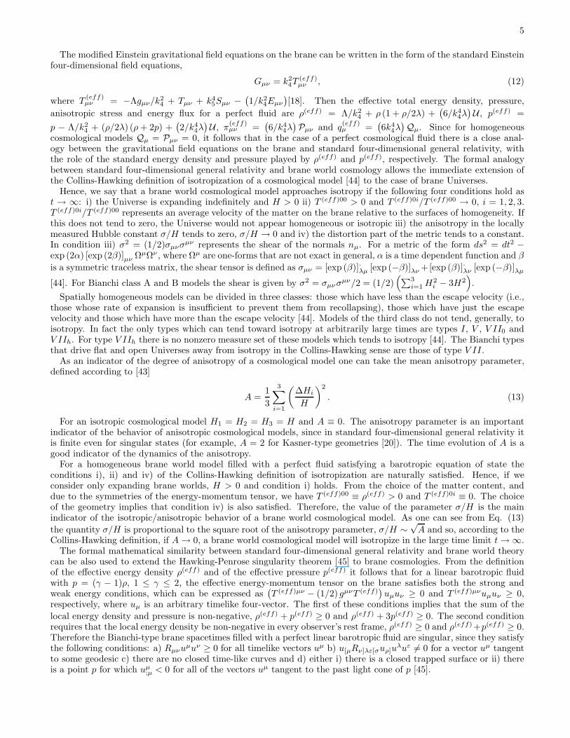
Qµ. Since for homogeneouscosmological models Qµ = Pµν = 0, it follows that in the case of a perfect cosmological fluid there is a close anal-ogy between the gravitational field equations on the brane and standard four-dimensional general relativity, withthe role of the standard energy density and pressure played by ρ(eff) and p(eff), respectively. The formal analogybetween standard four-dimensional general relativity and brane world cosmology allows the immediate extension ofthe Collins-Hawking definition of isotropization of a cosmological model [44] to the case of brane Universes.

Hence, we say that a brane world cosmological model approaches isotropy if the following four conditions hold ast → ∞: i) the Universe is expanding indefinitely and H > 0 ii) T (eff)00 > 0 and T (eff)0i/T (eff)00 → 0, i = 1, 2, 3.T (eff)0i/T (eff)00 represents an average velocity of the matter on the brane relative to the surfaces of homogeneity. Ifthis does not tend to zero, the Universe would not appear homogeneous or isotropic iii) the anisotropy in the locallymeasured Hubble constant σ/H tends to zero, σ/H → 0 and iv) the distortion part of the metric tends to a constant.In condition iii) σ2 = (1/2)σµνσµν represents the shear of the normals nµ. For a metric of the form ds2 = dt2 −exp (2α) [exp (2β)]µν ΩµΩν , where Ωµ are one-forms that are not exact in general, α is a time dependent function and β

is a symmetric traceless matrix, the shear tensor is defined as σµν = [exp (β)].λµ [exp (−β)]λν +[exp (β)]

.λν [exp (−β)]λµ

[44]. For Bianchi class A and B models the shear is given by σ2 = σµνσµν/2 = (1/2)(

∑3i=1 H2

i − 3H2)

.

Spatially homogeneous models can be divided in three classes: those which have less than the escape velocity (i.e.,those whose rate of expansion is insufficient to prevent them from recollapsing), those which have just the escapevelocity and those which have more than the escape velocity [44]. Models of the third class do not tend, generally, toisotropy. In fact the only types which can tend toward isotropy at arbitrarily large times are types I, V , V II0 andV IIh. For type V IIh there is no nonzero measure set of these models which tends to isotropy [44]. The Bianchi typesthat drive flat and open Universes away from isotropy in the Collins-Hawking sense are those of type V II.

As an indicator of the degree of anisotropy of a cosmological model one can take the mean anisotropy parameter,defined according to [43]

A =1

3

3∑

i=1

(

∆Hi

H

)2

. (13)

For an isotropic cosmological model H1 = H2 = H3 = H and A ≡ 0. The anisotropy parameter is an importantindicator of the behavior of anisotropic cosmological models, since in standard four-dimensional general relativity itis finite even for singular states (for example, A = 2 for Kasner-type geometries [20]). The time evolution of A is agood indicator of the dynamics of the anisotropy.

For a homogeneous brane world model filled with a perfect fluid satisfying a barotropic equation of state theconditions i), ii) and iv) of the Collins-Hawking definition of isotropization are naturally satisfied. Hence, if weconsider only expanding brane worlds, H > 0 and condition i) holds. From the choice of the matter content, anddue to the symmetries of the energy-momentum tensor, we have T (eff)00 ≡ ρ(eff) > 0 and T (eff)0i ≡ 0. The choiceof the geometry implies that condition iv) is also satisfied. Therefore, the value of the parameter σ/H is the mainindicator of the isotropic/anisotropic behavior of a brane world cosmological model. As one can see from Eq. (13)

the quantity σ/H is proportional to the square root of the anisotropy parameter, σ/H ∼√

A and so, according to theCollins-Hawking definition, if A → 0, a brane world cosmological model will isotropize in the large time limit t → ∞.

The formal mathematical similarity between standard four-dimensional general relativity and brane world theorycan be also used to extend the Hawking-Penrose singularity theorem [45] to brane cosmologies. From the definitionof the effective energy density ρ(eff) and of the effective pressure p(eff) it follows that for a linear barotropic fluidwith p = (γ − 1)ρ, 1 ≤ γ ≤ 2, the effective energy-momentum tensor on the brane satisfies both the strong andweak energy conditions, which can be expressed as

(

T (eff)µν − (1/2) gµνT (eff))

uµuν ≥ 0 and T (eff)µνuµuν ≥ 0,respectively, where uµ is an arbitrary timelike four-vector. The first of these conditions implies that the sum of the

local energy density and pressure is non-negative, ρ(eff) + p(eff) ≥ 0 and ρ(eff) + 3p(eff) ≥ 0. The second conditionrequires that the local energy density be non-negative in every observer’s rest frame, ρ(eff) ≥ 0 and ρ(eff)+p(eff) ≥ 0.Therefore the Bianchi-type brane spacetimes filled with a perfect linear barotropic fluid are singular, since they satisfythe following conditions: a) Rµνuµuν ≥ 0 for all timelike vectors uµ b) u[µRν]λε[σuρ]u

λuε 6= 0 for a vector uµ tangentto some geodesic c) there are no closed time-like curves and d) either i) there is a closed trapped surface or ii) thereis a point p for which uµ

;µ < 0 for all of the vectors uµ tangent to the past light cone of p [45].

6

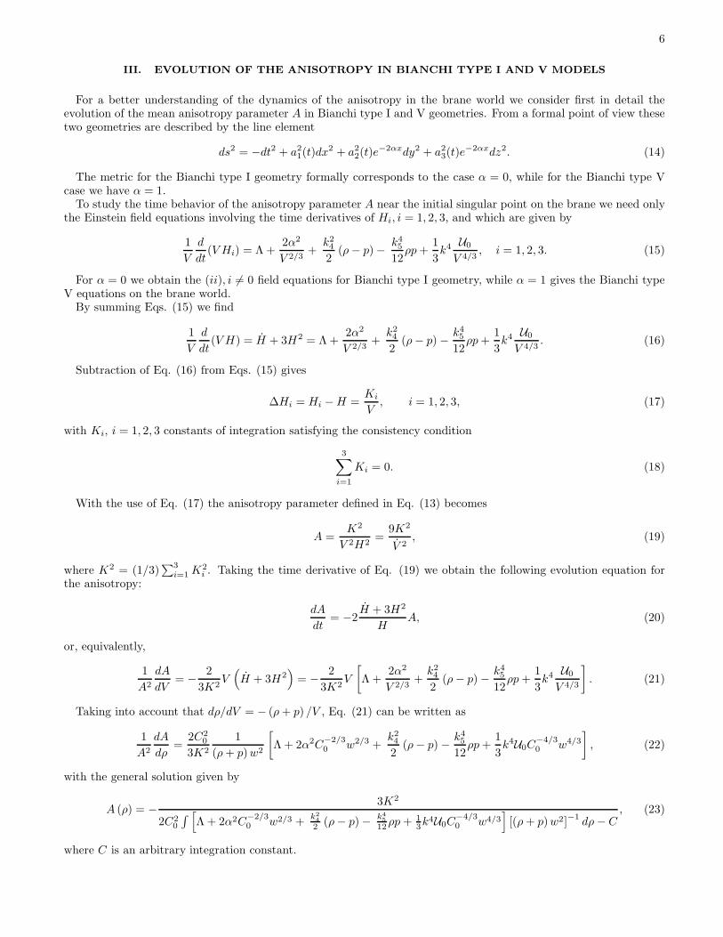
III. EVOLUTION OF THE ANISOTROPY IN BIANCHI TYPE I AND V MODELS

For a better understanding of the dynamics of the anisotropy in the brane world we consider first in detail theevolution of the mean anisotropy parameter A in Bianchi type I and V geometries. From a formal point of view thesetwo geometries are described by the line element

ds2 = −dt2 + a21(t)dx2 + a2

2(t)e−2αxdy2 + a2

3(t)e−2αxdz2. (14)

The metric for the Bianchi type I geometry formally corresponds to the case α = 0, while for the Bianchi type Vcase we have α = 1.

To study the time behavior of the anisotropy parameter A near the initial singular point on the brane we need onlythe Einstein field equations involving the time derivatives of Hi, i = 1, 2, 3, and which are given by

1

V

d

dt(V Hi) = Λ +

2α2

V 2/3+

k24

2(ρ − p) − k4

5

12ρp +

1

3k4 U0

V 4/3, i = 1, 2, 3. (15)

For α = 0 we obtain the (ii), i 6= 0 field equations for Bianchi type I geometry, while α = 1 gives the Bianchi typeV equations on the brane world.

By summing Eqs. (15) we find

1

V

d

dt(V H) = H + 3H2 = Λ +

2α2

V 2/3+

k24

2(ρ − p) − k4

5

12ρp +

1

3k4 U0

V 4/3. (16)

Subtraction of Eq. (16) from Eqs. (15) gives

∆Hi = Hi − H =Ki

V, i = 1, 2, 3, (17)

with Ki, i = 1, 2, 3 constants of integration satisfying the consistency condition

3∑

i=1

Ki = 0. (18)

With the use of Eq. (17) the anisotropy parameter defined in Eq. (13) becomes

A =K2

V 2H2=

9K2

V 2, (19)

where K2 = (1/3)∑3

i=1 K2i . Taking the time derivative of Eq. (19) we obtain the following evolution equation for

the anisotropy:

dA

dt= −2

H + 3H2

HA, (20)

or, equivalently,

1

A2

dA

dV= − 2

3K2V(

H + 3H2)

= − 2

3K2V

[

Λ +2α2

V 2/3+

k24

2(ρ − p) − k4

5

12ρp +

1

3k4 U0

V 4/3

]

. (21)

Taking into account that dρ/dV = − (ρ + p) /V , Eq. (21) can be written as

1

A2

dA

dρ=

2C20

3K2

1

(ρ + p)w2

[

Λ + 2α2C−2/30 w2/3 +

k24

2(ρ − p) − k4

5

12ρp +

1

3k4U0C

−4/30 w4/3

]

, (22)

with the general solution given by

A (ρ) = − 3K2

2C20

∫

[

Λ + 2α2C−2/30 w2/3 +

k2

4

2 (ρ − p) − k4

5

12ρp + 13k4U0C

−4/30 w4/3

]

[(ρ + p)w2]−1 dρ − C, (23)

where C is an arbitrary integration constant.

7

Eq. (23) gives the general representation of the anisotropy parameter as a function of the energy density of thecosmological fluid for the Bianchi type I and V space-times in the brane world scenario. For a cosmological fluid forwhich the thermodynamic pressure p obeys a linear barotropic equation of state of the form p = (γ − 1)ρ, γ = const.,1 ≤ γ ≤ 2, we have ρ = ρ0/V γ , with ρ0 ≥ 0 a constant of integration. ρ0 can be expressed in terms of C0 as ρ0 = Cγ

0 .Hence the anisotropy equation Eq. (23) can be immediately integrated to give the general exact dependence of theanisotropy parameter on the volume scale factor for Bianchi type I and V geometries:

A (V ) =3K2

ΛV 2 + 3α2V 4/3 + k24ρ0V 2−γ +

k4

5

12ρ20V

2−2γ + k4U0V 2/3 + C, (24)

where the arbitrary integration constant C 6= 0 is related, via the field equations, to the constant K2 by the relationC = 2K2/3 [27]. The singular state at t = 0 is characterized by the condition V (0) = 0. The value of the anisotropyparameter for t = 0 depends on the equation of state of the cosmological fluid. Hence for 1 < γ ≤ 2, from Eq. (24) itfollows

limV →0

A (V ) = 0, 1 < γ ≤ 2. (25)

Therefore the singular state of the high density Bianchi type I and V brane cosmological models is isotropic, withA(0) = 0. For the case of the pressureless dust filled anisotropic brane Universes, p = 0 and γ = 1. In this case

limV →0

A (V ) =36K2

k45ρ

20 + 12C

, γ = 1. (26)

The singular state of the dust filled brane Universe is anisotropic, with A(0) 6= 0. In the case of the standardfour-dimensional general relativity (SGR), the behavior of the anisotropy parameter is different from the case ofbrane cosmological models. SGR is recovered if the limits k5 → 0, k → 0 and Λ5 → −∞ are taken simultaneously.Therefore the anisotropy parameter in standard four-dimensional general relativity ASGR is given by

ASGR (V ) =3K2

(

ΛV 2 + 3α2V 4/3 + k24ρ0V 2−γ + C

) . (27)

Near the singular state,

limV →0

ASGR (V ) =3K2

C> 0, ∀γ ∈ [1, 2] . (28)

In fact, one can show that for barotropic matter filled standard four-dimensional general relativistic Bianchi type Iand V models ASGR (0) ≤ 2 [27].

Therefore in the case γ = 1 we obtain the following relation between the initial values of the anisotropy parametersA and ASGR of the brane world models and of the SGR, respectively:

A(0) =ASGR(0)

1 +k4

5ρ2

0

12C

. (29)

In Bianchi type I and V geometries there is also a simple proportionality relation between the shear scalar σ2 andthe anisotropy parameter:

σ2 = σikσik/2 =1

2

(

3∑

i=1

H2i − 3H2

)

=3

2AH2. (30)

IV. BEHAVIOR OF ANISOTROPY IN ARBITRARY TYPE BIANCHI MODELS

For arbitrary type Bianchi geometries the (ii) , i = 1, 2, 3 components of the gravitational field equations on thebrane can be represented in the following general form:

1

V

d

dt(V Hi) = Fi (a1, a2, a3) + Λ +

k24

2(ρ − p) − k4

5

12ρp +

1

3k4 U0

V 4/3, i = 1, 2, 3, (31)

8

Bianchi type c1 c2 c3

I 0 0 0

II 1 0 0

VI0 1 -1 0

VII0 1 1 0

VIII 1 1 -1

IX 1 1 1

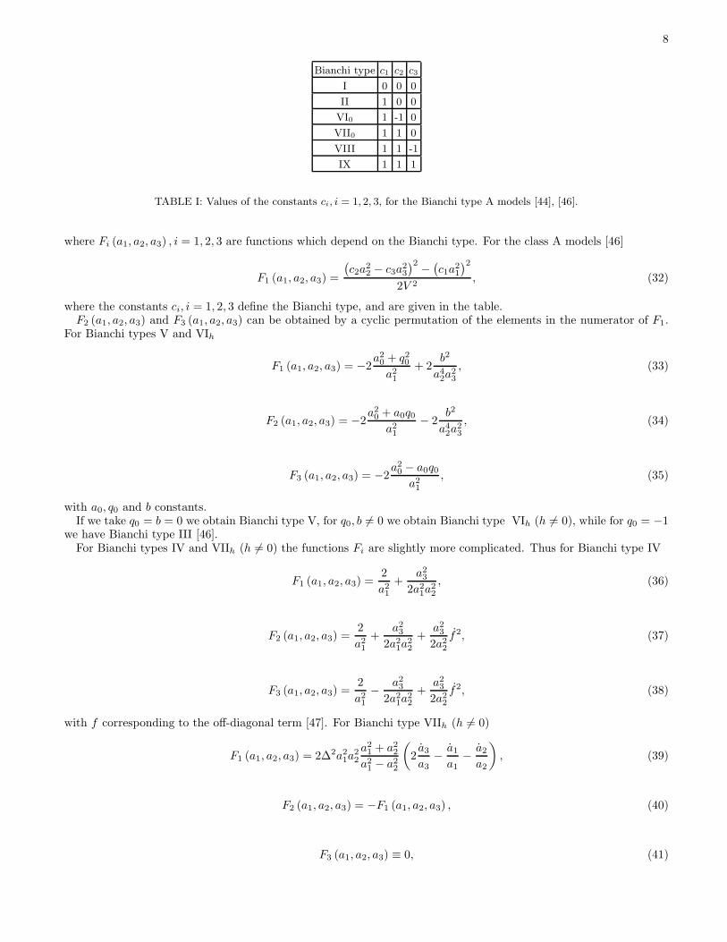
TABLE I: Values of the constants ci, i = 1, 2, 3, for the Bianchi type A models [44], [46].

where Fi (a1, a2, a3) , i = 1, 2, 3 are functions which depend on the Bianchi type. For the class A models [46]

F1 (a1, a2, a3) =

(

c2a22 − c3a

23

)2 −(

c1a21

)2

2V 2, (32)

where the constants ci, i = 1, 2, 3 define the Bianchi type, and are given in the table.F2 (a1, a2, a3) and F3 (a1, a2, a3) can be obtained by a cyclic permutation of the elements in the numerator of F1.

For Bianchi types V and VIh

F1 (a1, a2, a3) = −2a20 + q2

0

a21

+ 2b2

a42a

23

, (33)

F2 (a1, a2, a3) = −2a20 + a0q0

a21

− 2b2

a42a

23

, (34)

F3 (a1, a2, a3) = −2a20 − a0q0

a21

, (35)

with a0, q0 and b constants.If we take q0 = b = 0 we obtain Bianchi type V, for q0, b 6= 0 we obtain Bianchi type VIh (h 6= 0), while for q0 = −1

we have Bianchi type III [46].For Bianchi types IV and VIIh (h 6= 0) the functions Fi are slightly more complicated. Thus for Bianchi type IV

F1 (a1, a2, a3) =2

a21

+a23

2a21a

22

, (36)

F2 (a1, a2, a3) =2

a21

+a23

2a21a

22

+a23

2a22

f2, (37)

F3 (a1, a2, a3) =2

a21

− a23

2a21a

22

+a23

2a22

f2, (38)

with f corresponding to the off-diagonal term [47]. For Bianchi type VIIh (h 6= 0)

F1 (a1, a2, a3) = 2∆2a21a

22

a21 + a2

2

a21 − a2

2

(

2a3

a3− a1

a1− a2

a2

)

, (39)

F2 (a1, a2, a3) = −F1 (a1, a2, a3) , (40)

F3 (a1, a2, a3) ≡ 0, (41)

9

where ∆ =constant6= 0 [48].Generally there is one more field equation, the (00) equation, but it will not be used in the proof of the results.By adding Eqs. (31) on obtains

1

V

d

dt(V H) = H + 3H2 = F (a1, a2, a3) + Λ +

k24

2(ρ − p) − k4

5

12ρp +

1

3k4 U0

V 4/3, (42)

where

F (a1, a2, a3) =1

3

3∑

i=1

Fi (a1, a2, a3) . (43)

Substraction of Eq. (42) from Eq. (31) and integration of the resulting equation gives

∆Hi = Hi − H =Ki

V+

1

3V

∫

∆Fi [a1 (V ) , a2 (V ) , a3 (V )]

HdV, i = 1, 2, 3, (44)

where

∆Fi (a1, a2, a3) = Fi (a1, a2, a3) − F (a1, a2, a3) , i = 1, 2, 3, (45)

with the property

3∑

i=1

∆Fi (a1, a2, a3) = 0, (46)

and Ki, i = 1, 2, 3 are constants of integration satisfying the condition∑3

i=1 Ki = 0.Therefore for an arbitrary Bianchi type geometry the anisotropy parameter can be represented in the following

exact form:

A =K2 + G2 + L

V 2H2= 9

K2 + G2 + L

V 2, (47)

where

K2 =1

3

3∑

i=1

K2i , (48)

G2 =1

27

3∑

i=1

[∫

∆Fi

HdV

]2

, (49)

and

L =2

9

3∑

i=1

Ki

∫

∆Fi

HdV. (50)

Taking the time derivative of Eq. (47), and changing the time variable to V , it follows that in an arbitrary Bianchitype geometry the anisotropy parameter satisfies a Bernoulli type first order differential equation of the form

dA

dV=

[

d

dVln(

K2 + G2 + L)

]

A −

2V

3 (K2 + G2 + L)

[

F (a1, a2, a3) + Λ +k24

2(ρ − p) − k4

5

12ρp +

1

3k4 U0

V 4/3

]

A2, (51)

with the general solution given by

A (V ) =3(

K2 + G2 + L)

∫

V[

F (a1, a2, a3) + Λ +k2

4

2 (ρ − p) − k4

5

12ρp + 13k4U0V −4/3

]

dV + C, (52)

10

where C is an arbitrary constant of integration.For a brane cosmological fluid obeying a linear barotropic equation of state p = (γ − 1) ρ, the anisotropy parameter

for arbitrary Bianchi type cosmological models is given by

A (V ) =3V 2γ

(

K2 + G2 + L)

V 2γ∫

V F [a1 (V ) , a2 (V ) , a3 (V )] dV + ΛV 2(1+γ) + k24ρ0V 2+γ +

k4

5

12 ρ20V

2 + k4U0V 2(1/3+γ) + CV 2γ, (53)

We shall consider in the following the behavior of the anisotropy parameter for arbitrary type Bianchi space-times,filled with a linear barotropic cosmological fluid, obeying an equation of state of the form p = (γ−1)ρ, 1 ≤ γ ≤ 2. Forthis form of cosmological matter the conditions ρ(eff) > 0, ρ(eff) + p(eff) > 0 and ρ(eff) + 3p(eff) > 0 are satisfiedon the brane. Therefore the corresponding cosmological models are singular [45]. Since in most Bianchi types onedoes not know any exact solution, in order to find the behavior of the anisotropy at early times, it is necessary touse some asymptotic solutions obtained, near the singularity, by approximate methods, in the limit of small values ofthe time parameter. In standard four-dimensional general relativity it is concluded that for all Bianchi types thereexists a Kasner-like ”vacuum phase” near the singularity, that is, in general, Einstein’s vacuum equations are thefirst order approximation of the equations with a nonvanishing matter term for t → 0. This idea has been proposeda long time ago by Belinskii, Lifshitz and Khalatnikov [49]. The general argument comes from the consideration ofa Kasner type metric ds2 = dt2 − tp1dx2 − tp2dy2 − tp3dz2, with pi, i = 1, 2, 3 constants satisfying the conditions∑3

i=1 pi =∑3

i=1 p2i = 1. For a linear barotropic equation of state it follows from the Bianchi identity (8) that energy

density of the matter behaves like ρ ∼ t−γ(p1+p2+p3). Therefore for asymptotes fulfilling the Kasner constraints thematter term may be neglected in comparison with terms coming from the geometric part of the field equations andcontaining the second time derivatives. A Kasner type behavior near the singularity for a Bianchi type IX braneworld geometry has been discussed in [28]

From Eq. (53) one can derive the behavior of the anisotropy parameter near the singular state on the brane for allBianchi types. We suppose that the brane Universe starts its evolution from a singular state, with ai (0) = 0, i = 1, 2, 3.For t > 0 and for an expanding geometry, the scale factors are monotonically increasing functions of time, which forsmall t can be represented in the Kasner form

ai ∼ V mi , i = 1, 2, 3, (54)

with mi constants satisfying the conditions 0 ≤ mi < 1, i = 1, 2, 3 and∑3

i=1 mi = 1.The existence of a such a representation for the scale factors near the singular point on the brane has been explicitly

proven, in the case of Bianchi type I and V geometries, in [27]. The mean Hubble parameter behaves near the singularstate like H ∼ V −1.

With these assumptions it is easy to find the behavior of the integrals involving the functions Fi and Gi. ForBianchi class A models,

∫

V F [a1 (V ) , a2 (V ) , a3 (V )]dV can be written, near the singular point, as a sum of termsof the form V 4mi , i = 1, 2, 3 and V 2mi+2mj , i 6= j:

∫

V F [a1 (V ) , a2 (V ) , a3 (V )] dV =

3∑

i=1

αiV4mi +

3∑

i6=j=1

βijV2mi+2mj , (55)

where αi, i = 1, 2, 3 and βij , i, j = 1, 2, 3 are constants.Thus, for example, for the integral involving the function F1 (a1, a2, a3) we obtain

∫

V F1 (a1, a2, a3) dV =c22

8m2V 4m2 − c2c3

2 (m2 + m3)V 2(m2+m3) +

c23

8m3V 4m3 − c2

1

8m1V 4m1 . (56)

For the other Bianchi types, the integral is a sum of terms of the form V 2−2mi , i = 1, 2, 3 or V 2+2m3−2m1−2m2 andcyclic permutation of this term. Due to the relation m1 + m2 + m3 = 1 the last expression can be transformed to theform V 4mi , i = 1, 2, 3. In the limit V → 0, all these terms tend to zero.

The behavior of the function G2 and L can be analyzed in a similar way, and one can easily show that limV →0 G2 =limV →0 L = 0. Therefore for all Bianchi type cosmological models the anisotropy parameter on the brane has thegeneral property limV →0 A = 0. In the limit of large times, V → ∞ and all Bianchi models (except type VII)isotropize, with A → 0.

V. DISCUSSIONS AND FINAL REMARKS

The time evolution of the anisotropy parameter for a linear barotropic fluid in the brane world model is very differentfrom the standard four-dimensional general relativistic case. In homogeneous and anisotropic brane world models the

11

Universe starts from an isotropic state, with A = 0. The anisotropy of the Universe is increasing in time, and reachesa maximum value after a finite time tmax. For time intervals so that t > tmax, A is a decreasing function of time whichgenerally tends, in the large time limit, to zero. In standard four-dimensional general relativity the Universe startsits evolution from a singular state with maximum anisotropy and reaches, for all Bianchi models except type VII, anisotropic state for t → ∞ [44]. For Bianchi type I and V geometries the maximum value of the anisotropy parameteris obtained for values of the volume scale factor V satisfying the equation

2ΛV + 4α2V 1/3 + (2 − γ) k24ρ0V

1−γ +k45

6ρ20 (1 − γ)V 1−2γ +

2

3k4U0V

−1/3 = 0, (57)

which follows from the condition dA/dV = 0. In the case of the Bianchi type I brane filled with a stiff cosmologicalfluid (γ = 2), and for a negligible small cosmological constant, Λ = 0, the maximum value of the volume scale factoris given by

Vmax =

(

k45ρ2

0

4k4U0

)3/8

=

(

k44ρ

20

4U0

)3/8

. (58)

The maximum value of the anisotropy parameter is given by

Amax = A (Vmax) =3K2

k24ρ0 +

√

ρ0

8

k4

5U3/4

0

k3

4

+ C. (59)

The value of the cosmological time for which the A reaches its maximum value can be found from Eq. (16), and itis given by

tmax =

∫ Vmax

0

xdx√

Cx2 + 3k4U0x8/3 + k45ρ

20/4

. (60)

The integral in Eq. (60) cannot be expressed in a simple analytical form.If in the early stages of evolution of a stiff (γ = 2) cosmological fluid on a Bianchi type I brane the dark radiation

term can be neglected, as being negligible small, U0 ≈ 0, then the existence of a maximum of A also requires anon-zero cosmological constant, Λ 6= 0 For U0 = 0 the maximum value of the volume scale factor is given by

Vmax =

(

k45ρ

20

12Λ

)1/4

, (61)

and the time necessary for the brane Universe to reach this state is

tmax =

∫ Vmax

0

xdx√

3Λx4 + Cx2 +k4

5ρ2

0

4

=1

2√

3Λln

(

1 +

√

2k25ρ0

k25ρ0 + C√

3Λ

)

. (62)

The maximum value of the anisotropy parameter is, in this case,

Amax = A (Vmax) =3K2

ρ0

(

k24 +

√

Λ3 k4

5

)

+ C. (63)

This type of behavior of A, with an initial monotonically increasing evolution from zero up to a maximum value,followed by a decrease to zero, specific to brane world cosmological models, is a direct consequence of the presence,in the gravitational field equations, of the term quadratic in the energy density.

In the present paper we have considered in a systematic manner the time evolution of the anisotropy parameter Ain the framework of homogeneous, arbitrary Bianchi type brane world cosmological models, with the matter contentconsisting of a perfect barotropic cosmological fluid. For Bianchi type I and V exact representations of A can beobtained from the field equations and therefore the initial behavior of A can be explicitly derived from the study ofthe exact representation near the singularity. In order to obtain the form of A at the initial moment of the cosmologicalevolution for the other Bianchi types we have used the crucial assumption that near the singularity the metric of thebrane world is of Kasner type. For a ”normal” matter filled brane world, satisfying a linear barotropic equation ofstate, the behavior of A is very different from the standard four-dimensional general relativistic case. In this casethe anisotropy parameter has the remarkable property limt→0 A(t) = limt→∞ A(t) = 0, in sharp contrast to the SGRcase. However, in the case of pressureless dust, the initial values of the anisotropy parameter are identical in bothbrane world and standard four-dimensional general relativistic cosmological models.

12

Acknowledgments

The authors would like to thank to the two anonymous referees, whose comments helped to significantly improvethe manuscript.

[1] Randall L and Sundrum R 1999 Phys. Rev. Lett. 83 3370; hep-ph/9905221; Randall L and Sundrum R 1999 Phys. Rev.Lett 83 4690; hep-th/9906064

[2] Horava P and Witten E 1996 Nucl. Phys. B460 506; hep-th/9510209[3] Maartens R 2003 gr-qc/0312059

[4] Kim H B and Kim H D 2000 Phys. Rev. D61 064003; hep-th/9909053[5] Binetruy P, Deffayet C, Ellwanger U and Langlois D 2000 Phys. Lett. B477 285; hep-th/9910219[6] Binetruy P, Deffayet C and Langlois D 2000 Nucl. Phys. B565 269; hep-th/9905012[7] Stoica H, Tye S-H H and Wasserman I 2000 Phys. Lett. B482 205; hep-th/0004126[8] Langlois D, Maartens R and Wands D 2000 Phys. Lett. B489 259; hep-th/0006007[9] Kodama H, Ishibashi A and Seto O 2000 Phys. Rev. D62 064022; hep-th/0004160

[10] van de Bruck C, Dorca M, Brandenberger R H and Lukas A. 2000 Phys. Rev. D62 123515; hep-th/0005032[11] Csaki C, Erlich J, Hollowood T J and Shirman Y 2000 Nucl. Phys. B581 309; hep-th/0001033[12] Csaki C, Graesser M, Kolda C and Terning J 1999 Phys. Lett. B462 34 (1999); hep-ph/9906513[13] Cline J M, Grojean C and Servant G. 1999 Phys. Rev. Lett. 83 4245; hep-ph/9906523[14] Anchordoqui L, Nunez C and Olsen K 2000 JHEP 0010 050; hep-th/0007064[15] Shiromizu T, Maeda K and Sasaki M 2000 Phys. Rev. D62 024012; gr-qc/9910076[16] Sasaki M, Shiromizu T and Maeda K 2000 Phys. Rev. D62 024008; hep-th/9912233[17] Maeda K and Wands D 2000 Phys. Rev. D62 124009; hep-th/0008188[18] Maartens R 2000 Phys. Rev. D62 084023; hep-th/0004166[19] Maartens R, Sahni V and Saini T D 2001 Phys. Rev. D63 063509; gr-qc/0011105[20] Chen C-M, Harko T and Mak M K 2001 Phys. Rev. D64 124017; hep-th/0106263[21] Harko T and Mak M K 2003 Class. Quantum. Grav. 20 407[22] Chen C-M, Harko T, Kao W F and Mak M K 2002 Nucl. Phys. B636 159[23] Chen C-M, Harko T, Kao W F and Mak M K 2003 JCAP 11 005[24] Toporensky A V 2001 Class. Quantum. Grav. 18 2311; gr-qc/0103093[25] Campos A and Sopuerta C F 2001 Phys. Rev. D63 104012; hep-th/0101060[26] Campos A and Sopuerta C F 2001 Phys. Rev. D64 104011; hep-th/0105100[27] Chen C-M, Harko T and Mak M K 2001 Phys. Rev. D64 044013; hep-th/0103240[28] Coley A 2002 Phys. Rev. D66 023512; hep-th/0110049[29] Coley A 2002 Class. Quantum Grav. 19 L45; hep-th/0110117[30] Frolov A V 2001 Phys. Lett. B514 213; gr-qc/0102064[31] Santos M G, Vernizzi F and Ferreira P G 2001 Phys. Rev. D64 063506; hep-ph/0103112[32] Barrow J D and Hervik S 2002 Class. Quantum. Grav. 19 155; gr-qc/0109084[33] Barrow J D and Maartens R 2002 Phys. Lett. B532 153; gr-qc/0108073[34] Savchenko N Yu and Toporensky A V 2003 Class. Quantum. Grav. 20 2553; gr-qc/0212104[35] Campos A, Maartens R, Matravers D and Sopuerta C F 2003; hep-th/0308158[36] Aguirregabiria J M and Lazkoz R 2003, gr-qc/0304046[37] Aguirregabiria J M, Chimento L P and Lazkoz R 2003; gr-qc/0303096[38] Bruni M and Dunsby P K S 2002 Phys. Rev. D66 101301; hep-th/0207189[39] Coley A A, He Y, Lim W C 2003; gr-qc/0312075[40] Dunsby P, Goheer N, Bruni M, Coley A 2003; hep-th/0312174[41] Coley A A 2003; gr-qc/0312073[42] Maartens R 1996 astro-ph/9609119

[43] Caderni N and Fabbri R 1979 Phys. Rev. D20 1251[44] Collins C B and Hawking S W 1973 Astrophys. J. 180 317[45] Hawking S W and Ellis G F R 1995 The large scale structure of space-time, Cambridge University Press, London[46] Jensen L G and Stein-Schabes J A 1986 Phys. Rev. D34, 931[47] Harvey A and Tsoubelis D 1977 Phys. Rev. D15, 2734[48] von Borzeszkowski H-H and Muller V 1978 Ann. Phys. (Leipzig) 7 361[49] Belinskii V A, Lifshitz E M and Khalatnikov I M 1971 Sov. Phys. Usp. 13 745; Belinskii V A, Lifshitz E M and Khalatnikov

I M 1982 Adv. in Physics 31 639