Anisotropic tomography of the Atlantic Ocean from Rayleigh surface waves

Ž .Physics of the Earth and Planetary Interiors 106 1998 257–273

Anisotropic tomography of the Atlantic Ocean from Rayleighsurface waves

Graca Silveira a,b,c,), Eleonore Stutzmann d, Daphne-Anne Griot d,´ ´Jean-Paul Montagner d, Luis Mendes Victor a,b

a Centro de Geofısica da UniÕersidade de Lisboa, Rua da Escola Politecnica, 58, P-1250 Lisboa, Portugal´ ´b Departamento de Fısica da Faculdade de Ciencias, UniÕersidade de Lisboa, Edifıcio C1, Campo Grande, P-1700 Lisboa, Portugal´ ˆ ´

c Instituto Superior de Engenharia de Lisboa, Rua Conselheiro Emıdio NaÕarro, P-1800 Lisboa, Portugal´d Departement de Sismologie, Institut de Physique du Globe 4, place Jussieu, 75252 Paris Cedex 05, France´

Received 30 June 1997; accepted 24 December 1997

Abstract

The depth extent of the Mid Atlantic Ridge and the role of hotspots in the Atlantic opening are still a matter of debate. Inorder to constrain the structure and the geodynamic processes below the Atlantic Ocean, we provide the first anisotropicphase velocity maps of this area, obtained at a regional scale. We have determined Rayleigh wave phase velocities along1311 direct epicentre to station paths. For each path, phase velocities are calculated by a technique of cross-correlation witha synthetic seismogram. These phase velocities are corrected for the effect of shallow layers. They are then inverted, withouta priori constraints, to obtain maps of the lateral variations of the anisotropic phase velocities in the period range 50–250 s.The ridge axis corresponds to a low velocity anomaly, mainly visible at short periods. A good correlation between hotspotlocations and low velocity anomalies is obtained for the whole period range. Furthermore, a low velocity anomaly elongatedalong a North–South direction is visible for every period and seems to be correlated with hotspot positions. On average, theNorth Atlantic is associated with higher velocities than the South Atlantic. The shields below Canada, Brazil and Africadisplay high velocity anomaly at short periods and only the Brazilian and African shields are still visible for a period of 200s, thus suggesting that the Canadian shield is a shallower structure. The maps of phase velocity anisotropy under the AtlanticOcean are interpreted in the Mid-Atlantic area, where we have the best resolution. Close to the ridge, the fast axis ofRayleigh wave phase velocity is found perpendicular to the ridge axis. A comparison of anisotropy directions and platemotion shows that seismic anisotropy integrates also deeper phenomena such as mantle convection. q 1998 Elsevier ScienceB.V. All rights reserved.

Keywords: Anisotropic tomography; Atlantic ocean; Rayleigh surface waves; Mid Atlantic ridge

1. Introduction

The last re-opening of the Atlantic Ocean datesfrom about 180 Ma. With the exception of the

) Corresponding author.

Antilles and Sandwich islands, it is surrounded bypassive margins. Its most prominent feature is the

Ž .Mid Atlantic Ridge MAR which is found to be ashallow structure, visible only down to about 250 km

Ždepth on tomographic models Montagner and Tani-.moto, 1990, 1991 . It has a low spreading rate

0031-9201r98r$19.00 q 1998 Elsevier Science B.V. All rights reserved.Ž .PII S0031-9201 98 00079-X

( )G. SilÕeira et al.rPhysics of the Earth and Planetary Interiors 106 1998 257–273258

ranging from 1 to 4 cmryear and its origin at depthis not well established. Due to this low spreadingrate, the age of the ocean floor rapidly increases withthe distance from the ridge axis. The ridge axis has aNorth–South direction in the South Atlantic anddeviates to the West in the North Atlantic. A strikingfeature is the alignment of hotspots along a roughlyNorth–South direction in the whole Atlantic. Theyare located along the ridge axis in the South Atlanticbut off the ridge axis in the North Atlantic. A betterknowledge of their lateral and depth extent willenable us to understand their origin and their role inmantle convection.

During the last two decades, the development ofbroadband seismograph global networks, combinedwith the improvement of computers have enabledscientists to produce tomographic models of the Earthwith increasing resolution. The first generation ofmodels have only used the travel time or phase ofseismograms to provide isotropic models. Later, pa-rameterization of the anisotropy and anelasticity was

Žincluded in the models among others: Montagner,1986b; Montagner and Jobert, 1988; Bussy et al.,

.1993; Griot, 1997 . More recently, geodynamic con-Žstraints have been taken into account as in Forte et

.al., 1994 , and other models have been derived fromŽwaveform inversion among others; Stutzmann and

Montagner, 1994; Li and Romanowicz, 1996; De-.bayle and Leveque, 1997 . These models provide a´ ˆ

three dimensional image of the Earths mantle at aglobal scale as well as at a regional scale.

When comparing regions of similar ages, the am-plitude of velocity anomalies is always higher underthe Atlantic Ocean than under the Pacific OceanŽamong others: Montagner and Tanimoto, 1991; Ek-

.strom et al., 1997 . The ridge axis is the only striking¨feature when we zoom in on the Atlantic on globaltomographic models. Recently, Trampert and Wood-

Ž .house 1995, 1996 have obtained an almost continu-ous low phase velocity anomaly under the MAR forLove waves of periods larger than 79 s. This lowvelocity anomaly, however, is not so visible on theirRayleigh wave phase velocity maps, even at shortperiods. In contrast, the global Rayleigh wave phase

Ž .velocity maps of Ekstrom et al. 1997 display a¨nearly continuous low velocity anomaly along theMid-Atlantic Ridge for periods ranging from 50 to

Ž .150 s. On the other hand, the Zhang and Lay 1996

phase velocity maps provide velocity anomalies thatare not well correlated with the ridge axis.

Global tomographic models mainly enable us todistinguish the MAR and the oceanic basins. Smallscale features under the Atlantic Ocean can onlycome out from regional studies. Unfortunately, theAtlantic Ocean is not very suitable for regionaltomographic studies due to the lack of seismicity.Indeed, Mid-Atlantic ridge presents low seismic ac-tivity and there is little seismicity around the Ocean.

Ž .Weidner 1974 was the first to correlate regionallateral variations of surface wave phase velocitieswith different sediment thicknesses between ridges

Ž .and basins. Later, Canas and Mitchell 1981 relatedshear wave velocity anomalies to the age of the

Ž .Atlantic Ocean floor. Honda and Tanimoto 1987performed waveform inversion to obtain the firstregional three dimensional model of the AtlanticOcean. At shallow depths, they obtained low veloci-ties beneath the Azores triple junction and underEurope and high velocities beneath the Canadianshield and in the Central Atlantic. Mocquet et al.Ž .1989 confirm the existence of a high phase velocity

Ž .anomaly for periods larger than 100 s beneath theCentral Atlantic. Later, Mocquet and RomanowiczŽ .1990 , using surface wave phase velocities, and

Ž .Grand 1994 , using S-wave travel times, presentednew Atlantic regional three dimensional models. Wecan summarize robust features of all these models as

Ž .follows: 1 the North Atlantic lithosphere is charac-terized by slower velocities beneath the MAR than

Ž .under the old ocean basins; 2 the Atlantic astheno-sphere structure does not exhibit deep low velocityanomalies below the MAR and, furthermore, thecentral part of the ridge displays a high velocityanomaly for depths greater than 300 km.

The mapping of seismic velocity anomalies isgetting progressively consistent between differentstudies, but azimuthal anisotropy patterns are still a

Ž .matter of debate. Kuo et al. 1987 explain theirSS–S differential travel times in the North Atlanticby azimuthal anisotropy which is compatible with amantle flow in a North–South direction. This modelhowever is incompatible with results obtained by

Ž .Sheehan and Solomon 1991 by a combined inver-sion of SS–S differential travel times, geoid heightand bathymetric depth anomaly. Yang and FischerŽ .1994 explain the discrepancy between these two

( )G. SilÕeira et al.rPhysics of the Earth and Planetary Interiors 106 1998 257–273 259

studies by taking into account the variation ofSSVrSSH amplitude ratio. On the other hand, Kuo

Ž .and Forsyth 1992 study SKS splitting and findanisotropy amplitudes smaller than in previous stud-ies.

In order to improve lateral resolution of velocitymodels under the Atlantic Ocean and to provide thefirst maps of anisotropy directions on a regionalscale, we have performed a tomographic study ofthis area using Rayleigh wave phase velocities. Phasevelocities are calculated by a technique of cross-cor-relation with a synthetic seismogram for each path.These phase velocities are then corrected to take intoaccount the effect of shallow layers. In a secondstep, they are inverted, without a priori constraints,to obtain phase velocity lateral variations and anisot-ropy in the period range 50–250 s. The results arethen discussed in the framework of mantle convec-tion and evolution of the Atlantic Ocean.

2. Method

2.1. Phase Õelocity measurement

For each epicentre-to-station path, phase velocityis computed by cross-correlating the data with asynthetic seismogram. The synthetic seismogram iscomputed by normal mode summation for a givenreference Earth model, source parameters and instru-

Ž .mental response Woodhouse and Girnius, 1982 .The phase difference, fyf , between observed ando

synthetic seismograms gives the delay time t be-tween the two signals as a function of angular fre-quency v:

f v yf vŽ . Ž .odt v s 1Ž . Ž .

v

Then phase velocity V is computed using the follow-ing relation:

D Ds qdt 2Ž .

V v V vŽ . Ž .o

where D is the epicentral distance and V the refer-o

ence phase velocity.

2.2. Phase Õelocity error estimation

Errors on phase velocity determination for a givenepicentre-to-station path are mainly due to seismicsource uncertainties and instrument approximations.Errors due to instrumental response can be neglectedbecause new broadband instruments are well cali-brated. We take into account errors due to the sam-pling rate, that is dt s10 s. Only the direct paths1

between epicentre and station are used and, there-fore, the effect of lateral refraction can be neglected.Seismic source uncertainties can be estimated fromnuclear explosions. Mislocations of nuclear explo-sions give an upper limit of 20 km for the uncer-tainty on epicentral locations. Error on earthquakeorigin time is considered here together with error onsource time function, with dt s5 s.2

Different estimations of errors dt are assumed toi

be independent and Gaussian. The error estimationon slowness can be computed as follows:

1r221 1 d D2 2d 1rV s dts dt qd t qŽ . 1 2

D D V

3Ž .

where V is the phase velocity and D the epicentraldistance.

2.3. Regionalization

The fundamental mode phase velocity is com-puted for every path. In a second step, these phasevelocities are inverted to obtain, for each period, amap of phase velocity lateral variations and anisotro-py. Using Rayleigh’s principle combined with har-

Ž .monic tensor decomposition of Backus 1970 , SmithŽ .and Dahlen 1973 have shown that for a slight

anisotropic earth, the local phase velocity at a given


point M, can be expressed, for each angular fre-quency v, by:

V v , M ,c sV v , M 1qa v , M cos 2cŽ . Ž . Ž . Ž .o 1

qa v , M sin 2c qa v , MŽ . Ž . Ž .2 3

=cos 4c qa v , M sin 4cŽ . Ž . Ž .4

4Ž .

where c is the azimuth of the considered directionand a the coefficients of azimuthal anisotropy.i

Ž .Montagner and Nataf 1986 have shown thatRayleigh waves are mainly sensitive to 2 c-coeffi-cients. Therefore in the following, we have onlyinverted phase velocity for isotropic velocity givenby V and the 2 anisotropic coefficients a , a .o 1 2

The relation between average phase velocity for agiven path from the epicentre E to the station S, VŽ .v,c and local phase velocity at a position M canbe written:

D d sSsH

V v ,c V v , MŽ . Ž .E o

d sSyH

V v , MŽ .E o

= a v , M cos 2cŽ . Ž .1

qa v , M sin 2c 5Ž . Ž . Ž .2

Ž .Following Montagner 1986a , the under-de-termined problem is solved by using a continuousformulation of the inverse problem proposed by

Ž .Tarantola and Valette 1982 . Parameter p is a vec-tor composed of three independent distributions V ,o

a and a . The data, d, is the vector of measured1 2

phase velocities for all paths. The reference modelslowness is noted p and we have:o

p r yp rŽ . Ž .o

n nd d d siT y1s C r ,r G SŽ .Ý Ý H p i i i jopath Di iis1 js1

=d sj

d y G p r 6Ž . Ž .Hj j o j½ 5path Dj j

with

d s d si jTS sC qH G H C r ,r GŽ .i j d path i path p i j ji j i j oD Di j

Ž .where G is the Frechet derivative matrix of Eq. 5 ;C is the covariance matrix of the data. The matrixd

is diagonal and corresponds to the square of theŽerrors on slowness computed for each path using

.relation 3 ; C is the a priori covariance function onp o

the parameters. In order to regularize the inversion, itis necessary to introduce a correlation length, L ,corr

which depends on the path coverage of the Earth.This covariance function between 2 points r and r1 2

is defined by:

cos D y1r r1 2C r ,r ss r s r expŽ . Ž . Ž .p 1 2 1 2 2o Lcor

7Ž .

where s is the a priori error on the parameters at thelocation r and D is the epicentral distance.

The a posteriori error on the model is defined bythe square root of the diagonal term of the a posteri-

Ž .ori covariance matrix Tarantola and Valette, 1982 :

C r ,r sC r ,rŽ . Ž .post 1 2 p 1 2o

n nd d d siy C r ,rŽ .Ý Ý H p 1 2o Dpath iiis1 js1

=d sjy1 TG S G C r ,rŽ . Ž .i jH i j p 1 2o Dpath jj

8Ž .

3. Data

3.1. Data selection

We have selected events occurring at the Mid-Atlantic Ridge and all around the Atlantic Ocean,with a magnitude larger than 5.8 and a known cen-

Ž .troid moment tensor CMT . Unfortunately, the MARand Atlantic coast seismicity is characterized mostlyby earthquakes of magnitude smaller than 5.8 forwhich no CMT is computed and corresponding tosignal with a high noise level. Furthermore, there isan evident lack of broadband or long period digitalseismic stations in and around the Atlantic Ocean.Therefore, we have also used events from the westSouth American coast, the Mediterranean region andCentral Africa. We have selected 10 GEOSCOPE


and 25 IRIS seismic stations that are located close tothe Atlantic area and were operational between 1987and 1994. We have used both vertical and longitudi-

Ž .nal components of the VLP Very Long PeriodŽ .channel 0.1 Hz . The geographical distribution of

the 1311 paths used in this study is presented in Fig.1.

An example of the data and synthetic seismogramfor the vertical component recorded at the ECHseismic station, for the Peru earthquake of 15 April1991, is shown in Fig. 2a. The corresponding phasevelocity is plotted in Fig. 2b. We have considered

Žthe PREM model as a reference model Dziewonski.and Anderson, 1981 .

3.2. Tests on inÕersion reliability

Phase velocities have been inverted to obtainlateral variations and anisotropy, in the period range50–250 s.

We have performed the inversion for differentwindows of the study area in order to check that theperipheral areas do not affect the seismic velocitydistribution in the best resolved area, that being thecentral Atlantic. Results are presented for latitudesbetween 408S and 608N and for longitudes between1008W and 208E.

Inversion results are controlled by two parame-ters, the a priori error on parameters and the correla-

Fig. 1. Geographical distribution of the 1311 paths used in this study.


Ž .Fig. 2. Vertical seismogram recorded by station ECH Echery ofŽ .the Peru earthquake of 5 April 1991. a Comparison of observed

Ž .and synthetic seismograms. b Phase velocities as a function ofperiod. Dashed line and continuous line correspond respectively tothe observed and model phase velocities.

tion length. The a priori error on parameters corre-sponds to uncertainties on velocities and anisotropy,and defines the variation range of the model parame-ters. The correlation length L is directly related tocorr

the wavelength of the final model anomalies. In afirst approximation, it can be estimated from thesurface of the studied area, S, the number of data,n , and the number of inverted parameters, n , withd p

Ž .the relation Stutzmann and Montagner, 1994 :

Snp2L s 9Ž .corr nd

We obtain L ,5.28,580 km.corr

To check the reliability of the inversion, we haveperformed several inversions for different correlationlengths, L , and the a priori error on velocities,corr

s , and on anisotropy, s . For each inversion, wevel aniŽ .have computed: a the a posteriori error on veloci-

Ž . Ž .ties defined by Eq. 8 ; b the data misfit:

nd1 2S p s d yg p 10Ž . Ž . Ž .Ý i i( nd is1

Ž .where n is the number of data; and c the ampli-d

tude of the heterogeneities defined by

1r22H H V u ,w yV sinu du dwŽ .Ž .u w R oAs 11Ž .

H H sinu du dwu w

Ž .where V u ,w is the local phase velocity after in-RŽ .version in a point of coordinates u ,w , V is theo

Ž .mean phase velocity, and u ,w are, respectively, thelatitude and longitude.

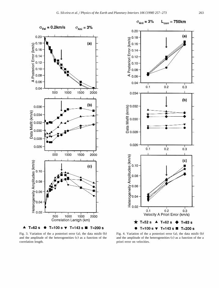
These three functions are presented as a functionof correlation length in Fig. 3, of velocity a priorierror in Fig. 4 and of anisotropy a priori error in Fig.5. The inverse problem is well resolved when the aposteriori error is smaller than the a priori error. Thea posteriori error and the data misfit have to be assmall as possible. Finally, the amplitude of hetere-geneities shows how phase velocity maps are per-

Žturbed by the inversion parameters correlation length.and a priori errors .

A good compromise between resolution and aposteriori errors corresponds to a correlation length

Ž .of 750 km Fig. 3a and b . Moreover, this correlationlength provides the largest amplitudes of the modelheterogeneities.

Fig. 4a shows that the a posteriori error on veloci-ties depends linearly on the velocity a priori error.The amplitude of heteregeneities also increases with

Ž .a priori error Fig. 4c . On the other hand, the datamisfit is not affected by this parameter in the rangeof 0.1–0.3 kmrs. This illustrates the difficulty ofresolving the absolute amplitude of velocities intomographic studies. We have therefore selected anintermediate value of 0.2 kmrs.

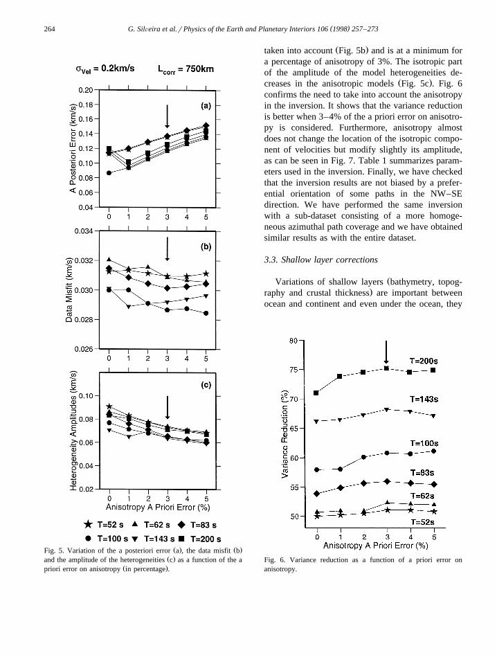
Fig. 5a shows that the velocity a posteriori errorsalso depends linearly on the anisotropy a priorierrors. The data misfit decreases when anisotropy is


Ž . Ž .Fig. 3. Variation of the a posteriori error a , the data misfit bŽ .and the amplitude of the heterogeneities c as a function of the

correlation length.

Ž . Ž .Fig. 4. Variation of the a posteriori error a , the data misfit bŽ .and the amplitude of the heterogeneities c as a function of the a

priori error on velocities.


Ž . Ž .Fig. 5. Variation of the a posteriori error a , the data misfit bŽ .and the amplitude of the heterogeneities c as a function of the a

Ž .priori error on anisotropy in percentage .

Ž .taken into account Fig. 5b and is at a minimum fora percentage of anisotropy of 3%. The isotropic partof the amplitude of the model heterogeneities de-

Ž .creases in the anisotropic models Fig. 5c . Fig. 6confirms the need to take into account the anisotropyin the inversion. It shows that the variance reductionis better when 3–4% of the a priori error on anisotro-py is considered. Furthermore, anisotropy almostdoes not change the location of the isotropic compo-nent of velocities but modify slightly its amplitude,as can be seen in Fig. 7. Table 1 summarizes param-eters used in the inversion. Finally, we have checkedthat the inversion results are not biased by a prefer-ential orientation of some paths in the NW–SEdirection. We have performed the same inversionwith a sub-dataset consisting of a more homoge-neous azimuthal path coverage and we have obtainedsimilar results as with the entire dataset.

3.3. Shallow layer corrections

ŽVariations of shallow layers bathymetry, topog-.raphy and crustal thickness are important between

ocean and continent and even under the ocean, they

Fig. 6. Variance reduction as a function of a priori error onanisotropy.


Fig. 7. Phase velocity perturbation maps obtained for a period of 100 s. They are computed with respect to the map average velocity andŽ . Ž .expressed in percent. a Isotropic inversion b–c–d Anisotropic inversion with an a priori error on anisotropy of 1%, 2% and 3%,

respectively.

vary as a function of sea floor age. Stutzmann andŽ .Montagner 1994 , among others, have shown that

the influence of Moho depth on fundamental modesurface waves is very important at short periods and

decreases with increasing periods. The frequencycontent of the data is dominantly long period andtherefore cannot resolve shallow structures. A pooraccount of these structures, however, can bias the


Table 1Parameters used in the inversion. s : data error; L : correla-data corr

tion length; s : a priori error on velocity; s : a priorivelocity anisotropy

error on anisotropy

Ž Ž ..s 0.02–0.08 kmrs see Eq. 3data

L 750 kmcorr

s 0.2 kmrsvelocity

s 3%anisotropy

deep structures. Therefore, the data have been cor-rected for crustal effect. Phase velocity crustal per-turbations have been computed for model 3SMACŽ .Nataf and Ricard, 1996 and subtracted from ourdata. The phase velocities have been corrected pathby path before inversion. As shown in Fig. 8, for aperiod of 62 s, the effect of shallow layer correctionincreases the amplitude of velocity anomalies butdoes not change their location. Moreover, shallow

layer correction does not change anisotropy ampli-tude and direction.

4. Results and discussion

4.1. Phase Õelocity distribution

Data corrected from the effect of shallow layershave been inverted using the a priori parameterspresented in Table 1. Maps of the isotropic compo-

Ž Ž ..nent of phase velocity, coefficient V in Eq. 4 ,o

are presented in Fig. 9 for several periods: 57, 100,167 and 200 s. In a first approximation, the periodcan be converted into the maximum depth sensitivityD using the relation DsTVr3, where T is theperiod and V is the phase velocity. The a posteriorierror maps are presented in Fig. 10 for the same

Ž .periods. At short periods Fig. 9a the phase velocity

Fig. 8. Phase velocity perturbation maps obtained for a period of 62 s. The perturbations are computed with respect to the map averageŽ . w x Ž .velocity V and expressed in percent. a without shallow layers corrections V s4.04 kmrs , b after shallow layer correctionsaverage average

w xV s4.08 kmrs .average


Fig. 9. Phase velocity perturbation maps obtained using the inversion parameters defined in Table 1. The perturbations are computed withŽ . Ž .respect to the map average velocity V and expressed in percent. a Ts57 s, V s4.07 kmrs; b Ts100 s, V s4.18average average average

Ž . Ž .kmrs; c Ts167 s V s4.46 kmrs; d Ts200 s; V s4.66 kmrs.average average


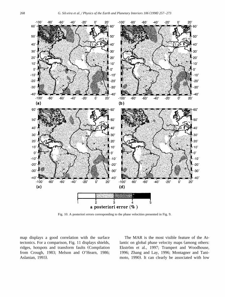
Fig. 10. A posteriori errors corresponding to the phase velocities presented in Fig. 9.

map displays a good correlation with the surfacetectonics. For a comparison, Fig. 11 displays shields,

Žridges, hotspots and transform faults Compilationfrom Crough, 1983; Melson and O’Hearn, 1986;

.Aslanian, 1993 .

The MAR is the most visible feature of the At-Žlantic on global phase velocity maps among others:

Ekstrom et al., 1997; Trampert and Woodhouse,¨1996; Zhang and Lay, 1996; Montagner and Tani-

.moto, 1990 . It can clearly be associated with low


Fig. 11. Plate boundaries, hotspot locations and some geologicalŽ . Ž .features-after Crough 1983 , Melson and O’Hearn 1986 , Asla-

Ž .nian 1993 . CSh, Canadian Shield; GSh, Guyana Shield; BSh,Brazilian Shield; WAc, West African craton; Cc, Congo craton.Circles designate hotspots, from top to bottom: AZ, Azores; M,Madeira; B, Bermuda; GM, Great Meteor; H, Hoggar; T, Tibesti;C, Canaries; CV, Cape Verde; CM, Cameroon; SL, Sierra Leone;Ž .Schilling et al., 1994 ; G, Galapagos; F, Fernando de Noronha;AS, Ascension; SH, Santa Helena; TD, Trindade; SF, San Felix;V, Vema; TC, Tristan da Cunha; JF, Juan Fernandez. Linescorrespond to hotspot traces.

Ž .velocities at short period Fig. 9a . We can followthe MAR as well as the Rio Grande rise, and theAzores–Gibraltar fracture zone. When period in-

Ž .creases Fig. 9b,c,d , the MAR becomes less visibleparticularly in the North Atlantic, where the positive

Ž .anomaly already visible at 57 s is shifted to theWest to become centered on the ridge axis. Thispositive anomaly is also reported by Mocquet et al.Ž . Ž1989 and Van Heijst personal communication,

.1997 and confirms the shallow origin of the ridge.The Rio Grande rise is reported as a hotspot track,and the Azores–Gibraltar fracture zone both have adeeper origin because they still correspond to a low

Žvelocity anomaly for periods of 167 and 200 s Fig..9c–d .

We can separate the structure of South and NorthAtlantic: the North Atlantic displays higher veloci-ties than the South Atlantic, meaning that it can beassociated with colder structures than the South At-

lantic. Moreover, for periods ranging from 50 to 170s, the South Atlantic displays an asymmetrical struc-ture with respect to the ridge, that is fast velocities atthe East and slow velocities at the West of the ridgeaxis. This asymmetry is, however, not so visible inthe North Atlantic.

A striking feature of the phase velocity maps isthe good correlation between low velocities and

Žhotspot surface locations plotted with a dot in Fig.. Ž9a–d up to the largest period inverted 200 s, that

.correspond roughly to 300–400 km depth . A lowvelocity anomaly is coming out, elongated in aroughly North–South direction that follows the pre-sent hotspot surface locations. In South Atlantic,hotspots are located along the ridge axis, and the lowvelocity anomaly coincide with this ridge axis. Incontrast, the low velocity anomaly in the NorthAtlantic is associated with hotspot locations and notwith the ridge axis.

The shields in Brazil, Canada and Africa, as wellas the oldest ocean basins in the North Atlanticcorrespond to high velocity anomalies at short pe-riod. When period increases, the Canadian shieldhigh velocity anomaly decreases significantly,whereas Brazilian and African shields still corre-spond to a strong positive amplitude even at a periodof 200 s. The positive anomaly beneath the Brazilianshield might be the trace at depth of the subductingplate.

Finally, the anomaly observed beneath theEurasian–African boundary, between Iberia andNorth Africa, is no longer visible beyond 100 sshowing that this is a shallow tectonic feature.

The results obtained by this regional study havebeen compared with the most recent global phasevelocity maps obtained by Trampert and WoodhouseŽ . Ž .1995, 1996 , Ekstrom et al. 1997 and Zhang and¨

Ž .Lay 1996 . Fig. 12 presents, for a period of 100 s,the isotropics models of Trampert and WoodhouseŽ . Ž .1996 , Ekstrom et al. 1997 and our anisotropic¨model. The three models have similar correlationlengths and the anomalies are expressed in percentwith respect to the PREM average velocity. Theamplitude of anomalies is stronger in our study thanin the global study because global models tend tofilter out short wavelength features, whereas ourregional maps maintain their presence. Although theprincipal features between the different models are


Ž . Ž . Ž .Fig. 12. Phase velocity perturbation maps for a period of 100 s. a Model of Trampert and Woodhouse 1996 ; b Model of Ekstrom et al.¨Ž . Ž .1997 ; c our model; phase velocity variations are given in percent with respect to the PREM average velocity of 4.089 kmrs.

consistent, the regional study gives a better resolu-tion of small features. The main discrepancy betweenmodels concerns the asymmetry of the ridge in the

ŽSouth Atlantic higher velocities at the East side than.at the West side of the ridge . This asymmetry is

observed in our model and is also reported by ZhangŽ .and Lay 1996 . We observe the same feature at long

period on the model from Trampert and Woodhouse

Ž . Ž .1995 , but Ekstrom et al. 1997 display a symmet-¨rical model with respect to the ridge.

4.2. Anisotropy directions

Data have been inverted for velocities and az-imuthal anisotropy. An anisotropy pattern is pre-sented in Fig. 13 for three periods: 57, 167 and


200 s. Anisotropy is plotted by a bar. The bardirection indicates Rayleigh wave fast direction,whereas, the bar length indicates the amplitude of theanisotropy.

The directions of the azimuthal fast axis ofŽ .Rayleigh waves Fig. 13 does not change much as a

function of period, but the amplitude of anisotropyincreases with increasing period. To resolve the ani-sotropy, it is necessary to have crossing paths com-

ing from different azimuths. Because of the pathŽ .distribution Fig. 1 , the well resolved area, in terms

of anisotropy, is limited to Central Atlantic. In thisarea, we observe a good relationship between theMid Atlantic ridge axis and anisotropy direction: thefast axis is perpendicular to the ridge and rotateswhen the ridge is curved. Under the Caribbean sea,we also observe a rotation of the fast direction whichmay reflect the direction of subduction. Finally, the

Ž . Ž . Ž .Fig. 13. Anisotropy Directions; a Ts57 s, b Ts167 s, c Ts200 s. A bar length of 5 mm corresponds to 2% of anisotropy.


western part of the North Atlantic shows a roughlyNorth–South fast direction that is in agreement with

Ž .the direction obtained by Kuo et al. 1987 fromshear waves. Fig. 13d shows the current plate veloci-ties relative to hotspots from Gripp and GordonŽ .1990 . A comparison of seismic anisotropy direc-tions with plate motion maps shows that anisotropydirections cannot be simply explained by plate mo-tion. This means that seismic anisotropy probablyintegrates deeper phenomena, such as mantle convec-tion.

5. Conclusions

The inversion of phase velocities obtained along1311 paths crossing the Atlantic Ocean has enabledus to obtain a model of phase velocity and azimuthalanisotropy lateral variations. We have shown thatanisotropy is necessary to explain the data. We haveobtained maps with a lateral resolution of about 800km. The phase velocity anomalies display strongeramplitudes than global tomographic models whichfilter out short wavelength features. Nevertheless, thelocation of anomalies is, in general, compatible withthe different models. On average, the North Atlanticcorresponds to higher velocities than the South At-lantic.

The ridge axis corresponds to a low velocityanomaly mainly visible at short period. A goodcorrelation between hotspot locations and low veloc-ity anomalies is obtained for the whole period range.Furthermore, a low velocity anomaly elongated alonga North–South direction is visible for every periodand seems to be correlated with hotspot positions.

The shields in Canada, Brazil and Africa corre-spond to high velocity anomalies at short period andonly the Brazilian and African shields are still visiblefor a period of 200 s. This suggest that the Canadianshield is a shallow structure with a maximum depthextent of about 150–200 km, whereas the Brazilianand African shields roots are deeper than 300 km.

Anisotropy directions are only interpreted in theMid-Atlantic area where they are best resolved. Thefast axis of Rayleigh waves is found to be perpendic-ular to the ridge axis. It rotates when the ridge iscurved. This anisotropy cannot be explained only by

plate motions, and probably integrates deeper phe-nomena, such as mantle convection.

In order to better quantify the depth extent andcharacterisation of hotspots, a combined inversion ofRayleigh and Love wave phase velocity is nowunder progress.

Acknowledgements

The authors would like to thank A. Forte and G.Roult for helpful discussions, and B. Forte for read-ing this paper. The research presented here wasperformed using data from the GEOSCOPE andIRIS seismograph networks. This work has beensupported by JNICTrCNRS Cooperation Program.This is IPGP contribution no. 1528.

References

Aslanian, D., 1993. Interactions entre les processus intraplaques etles processus d’accretion oceanique: l’apport du geoıde´ ´ ´ ¨altimetrique. PhD Thesis. Brest.´

Backus, G.E., 1970. A geometrical picture of anisotropic elastictensors. Rev. Geophys. 8, 633–671.

Bussy, M., Montagner, J.P., Romanowicz, B., 1993. Tomographicstudy of upper mantle attenuation in the Pacific Ocean. Geo-phys. Res. Lett. 20, 663–666.

Canas, J.A., Mitchell, B.J., 1981. Rayleigh wave attenuation andits variation across the Atlantic Ocean. Geophys. J. R. Astron.Soc. 67, 159–176.

Crough, S.T., 1983. Hotspot swells. Annu. Rev. Earth Planet Sci.11, 163–193.

Debayle, E., Leveque, J.J., 1997. Upper mantle heterogeneities in´ ˆthe Indian Ocean from waveform inversion. Geophys. Res.Lett. 24, 245–248.

Dziewonski, A.M., Anderson, D.L., 1981. Preliminary referenceEarth model. Phys. Earth Planet. Int. 25, 297–356.

Ekstrom, G., Tromp, J., Larson, E.W.F., 1997. Measurements and¨global models of surface waves propagation. J. Geophys. Res.102, 8137–8157.

Forte, A., Woodward, R.L., Dziewonski, A.M., 1994. Joint inver-sions of seismic and geodynamic data for models of three-di-mensional mantle heterogeneity. J. Geophys. Res. 99, 21857–21877.

Grand, S.P., 1994. Mantle shear structure beneath the Americasand surrounding. J. Geophys. Res. 99, 591–621.

Griot, D.A., 1997. Tomographie anisotrope de l’Asie Central apartir d’ondes de surface. These de doctorat de l’Universite de` ´Paris VII.

Gripp, A.E., Gordon, R.G., 1990. Current plate velocities relativeto the hotspots incorporating the NUVEL-1 global plate mo-tion model. Geophys. Res. Lett. 17, 1109–1112.


Honda, S., Tanimoto, T., 1987. Regional 3-D heterogeneities bywaveform inversion-application to the Atlantic area. Geophys.J. R. Astron. Soc. 94, 737–757.

Kuo, B.Y., Forsyth, D.W., 1992. A search for split SKS wave-forms in the North Atlantic. Geophys. J. Int. 108, 557–574.

Kuo, B.Y., Forsyth, D.W., Wysession, M., 1987. Lateral hetero-geneity and azimuthal anisotropy in the North Atlantic deter-mined from SS–S differential travel times. J. Geophys. Res.92, 6421–6436.

Li, X.D., Romanowicz, B., 1996. Global shear velocity modeldeveloped using non-linear asymptotic coupling theory. J.Geophys. Res. 101, 22245–22272.

Melson, W.G., O’Hearn, T., 1986. ‘Zero-age’ variations in thecomposition of abyssal volcanic rocks, The Geology of NorthAmerica, Vol. M., The Western North Atlantic Region, TheGeological Society of America, pp. 117–136.

Mocquet, A., Romanowicz, B., Montagner, J.P., 1989. Three-di-mensional structure of the upper mantle beneath the AtlanticOcean inferred from long-period Rayleigh waves: I. Groupand phase velocity distributions. J. Geophys. Res. 94, 7449–7468.

Mocquet, A., Romanowicz, B., 1990. Three-dimensional structureof the upper mantle beneath the Atlantic Ocean inferred fromlong-period Rayleigh waves: II. Inversion. J. Geophys. Res.95, 6787–6798.

Montagner, J.P., 1986a. Regional three-dimensional structuresŽ .using long period surface waves. Ann. Geophys. 4 B , 283–

294.Montagner, J.P., 1986b. First results on the three-dimensional

structure of the Indian Ocean inferred from long-period sur-face waves. Geophys. Res. Lett. 13, 315–318.

Montagner, J.P., Jobert, N., 1988. Vectorial tomography: II. Ap-plication to the Indian Ocean. Geophys. J. 94, 309–344.

Montagner, J.P., Nataf, H.C., 1986. A simple method for invertingthe azimuthal anisotropy of surface waves. J. Geophys. Res.91, 511–520.

Montagner, J.P., Tanimoto, T., 1990. Global anisotropy in theupper mantle inferred from the regionalization of phase veloci-ties. J. Geophys. Res. 95, 4797–4819.

Montagner, J.P., Tanimoto, T., 1991. Global upper mantle tomog-raphy of seismic velocities and anisotropies. J. Geophys. Res.96, 20337–20351.

Nataf, H.-C., Ricard, Y., 1996. 3-SMAC: A tomografic model ofthe upper mantle based on a geophysical modelling. Phys.Earth Planet Int. 95, 101–122.

Schilling, J.G., Hanan, B.B., McCully, B., Kingsley, R.H., 1994.Influence of the Sierra Leone mantle plume on the equatorialMid-Atlantic Ridge: a Nd–Sr–Pb isotopic study. J. Geophys.Res. 99, 12005–12028.

Sheehan, A.F., Solomon, S.C., 1991. Joint inversion of shearwave travel time residuals and geoid and depth anomalies forlong-wavelength variations in upper mantle temperature andcomposition along the Mid-Atlantic Ridge. J. Geophys. Res.96, 19981–20009.

Smith, M.L., Dahlen, F.A., 1973. The azimuthal dependence onLove and Rayleigh wave propagation in a slightly anisotropicmedium. J. Geophys. Res. 78, 3321–3333.

Stutzmann, E., Montagner, J.P., 1994. Tomography of the transi-tion zone from the inversion of higher-mode surface waves.Phys. Earth Planet. Int. 86, 99–116.

Tarantola, A., Valette, B., 1982. Generalized nonlinear inverseproblems solved using least squares criterion. Rev. Geophys.Space Phys. 20, 219–232.

Trampert, J., Woodhouse, J.H., 1995. Global phase velocity mapsof Love and Rayleigh waves between 40 and 150 seconds.Geophys. J. Int. 122, 675–690.

Trampert, J., Woodhouse, J.H., 1996. High resolution globalphase velocity distributions. Geophys. Res. Lett. 25, 21–24.

Weidner, D.J., 1974. Rayleigh wave phase velocities in the At-lantic Ocean. Geophys. J. R. Astron. Soc. 36, 105–139.

Woodhouse, J.H., Girnius, T.P., 1982. Surface waves and freeoscillations in a regionalized earth model. Geophys. J. R.Astron. Soc. 68, 653–673.

Yang, X., Fischer, K.M., 1994. Constraints on North Atlanticupper mantle anisotropy from S and SS phases. Geophys. Res.Lett. 21, 209–312.

Zhang, Y.S., Lay, T., 1996. Global surface wave phase velocityvariations. J. Geophys. Res. 101, 8415–8436.

Anisotropic tomography of the Atlantic Ocean from Rayleigh surface waves

Documents