AndersSchreiber_ThesisFinal

F A C U L T Y O F S C I E N C E U N I V E R S I T Y O F C O P E N H A G E N

Bachelor’s ThesisAnders Øhrberg Schreiber

Bounds on the Dimensionality of Space

N. Emil J. Bjerrum-Bohr

January 8, 2015

Abstract

In this thesis we expand on well known physical models with the purpose of setting bounds onthe dimensionality of space. We develop a D dimensional extension to the Schwarzschild metric ingeneral relativity. With this model, we set a dimension of space to be 3+ ε to investigate boundson a fractal dimensional deviation from three dimensions. Using data for perihelion precessionof binary pulsar systems, we find bounds on ε to be consistent with zero. Next we investigatethe possibility of using bending of light and gravitational redshift for the same purpose, butthese are not suitable for setting better bounds on ε. In quantum mechanics we set up a Ddimensional extension to a hydrogen-like system with a Coulomb interaction. Using spectraldata we find bounds on ε to be consistent with zero. The best upper bound on ε was foundfrom perihelion precession of PSR J0737-3039A to be |ε| < 5.0 · 10−9. Finally we investigatea hydrogen-like system with a compact extra dimension where the Coulomb potential does notlive in the extra dimension. With this model we set upper bounds on the radius of the extradimension, where the best upper bound on the radius of two extra dimensions of equal size isfound to be R < 6.11 ·10−13 m. We also investigate what happens if the Coulomb potential livesin the extra dimension and find that this model does not work.

University of Copenhagen email: [email protected]

Contents

1 Introduction 4

2 Schwarzschild phenomenology in fractal dimensional space 52.1 The Schwarzschild metric in D spatial dimensions . . . . . . . . . . . . . . . . . . . 52.2 Perihelion precession . . . . . . . . . . . . . . . . . . . . . . . . . . . . . . . . . . . . 62.3 Bending of light . . . . . . . . . . . . . . . . . . . . . . . . . . . . . . . . . . . . . . . 82.4 Gravitional redshift . . . . . . . . . . . . . . . . . . . . . . . . . . . . . . . . . . . . . 11

3 Hydrogen-like atoms in fractal and compactified space 123.1 Fractal dimensional space . . . . . . . . . . . . . . . . . . . . . . . . . . . . . . . . . 123.2 Compactification on S1: V (r) ∼ 1/r ∈ R3 . . . . . . . . . . . . . . . . . . . . . . . . 153.3 Changing the potential domain: V (r) ∼ 1/r ∈ R3 × S1 . . . . . . . . . . . . . . . . . 17

4 Summary and outlook 19

5 Appendix A: Christoffel symbols for the Schwarzschild metric 20

6 Appendix B: Perihelion precession derivation steps 21

7 Appendix C: Derivatives in the radial Schrodinger equation 22

8 Appendix D: Evaluating the potential with the method of images 24

References 26

1 Introduction Anders Øhrberg Schreiber

1 Introduction

In physics we explore the natural world through experiments and as a science it is common placeto question our knowledge again and again. Through this iterative process amazing discoverieshas occured over the past 500 years. In this thesis we will question one of the most incarnatedassumptions in science in general, namely that the universe has three spatial dimensions. If thishypothesis can be rejected, it will have profound consequences for the way we do physics and ourunderstanding of nature.

Many theorists believe that string theory [1] is the best way to unify general relativity with quantummechanics and solve the problems of the Standard Model of Particle Physics [2]. In string theory itis a requirement that we have more than three spatial dimensions [1] and it is therefore interesting toinvestigate whether or not this is actually the case in nature, as this would be a testable predictionfrom string theory.

We are going to be looking at well known phenomenology and want to understand if our currentlyaccepted models are fitting measurements well or if there is room for error, either ruling out modelsor implying the presence of a deviation from three dimensions. The notion of a fractal dimensionalspace is mathematically well defined [3] and one could therefore imagine a fractal deviation fromthree dimensions. Compact extra dimensions are also mathematically well defined [1]. We will beinvestigating both possibilities as extensions of models in both general relativity and non-relativisticquantum mechanics.

This thesis is divided into two main sections:

Part 1 In the first part of this thesis we are investigating how the presence of a fractal dimensionaldeviation from three spatial dimensions, i.e. D = 3+ε for some presumably small ε, will affectphysical models in the context of general relativity. We are considering the simple case of acompletely spherically symmetric and static system, i.e. a higher dimensional generalizationof the Schwarzschild metric. Using currently known astrophysical phenomenology we can setbounds on ε and see if we can reject the null hypothesis that ε = 0.

Part 2 In the second part of this thesis we are looking for a fractal deviation from three spatial dimen-sions in the context of non-relativistic quantum mechanics. We are considering a sphericallysymmetric system, i.e. a higher dimensional generalization of the hydrogen atom. From thespectrum we will to set bounds on ε and see if we can reject the null hypothesis that ε = 0.

Next up we will be looking at a quantum mechanical system that is spherically symmetric inthree dimensions and has a compact extra dimension. Considering first a potential that livesonly in R3, we will be looking at the spectrum for this system and, from ionization energies forhydrogen-like atoms, set upper bounds on the size of the compact extra dimension. Finallywe investigate what happens if the potential lives in all the dimensions R3 × S1 and here wesee that we can treat the potential in the extra dimension as a perturbation.

When investigating fractal dimensional deviations from three dimensions, we will take a null hy-pothesis that ε = 0 and see if we can reject this with measurements of upper bounds on ε. We willnot do hypothesis testing when investigating compactified extra dimensions.

4

2 Schwarzschild phenomenology in fractal dimensional space Anders Øhrberg Schreiber

2 Schwarzschild phenomenology in fractal dimensional space

In this section we consider the effects of a fractal dimensional space with 3 + ε spatial dimen-sions in the context of the spherically symmetric and static model in general relativity, namelythe Schwarzschild metric. We will derive the Schwarzschild metric in D spatial dimensions andone timelike dimension and consider phenomenology where we take D = 3 + ε and consider theeffect of small ε. This includes perihelion precession of a massive test particle, bending of light andgravitational redshift.

The reason why we only consider small ε deviations is that models in physics always assume threespatial dimensions and the success of physics under this assumption has been remarkable. Onlya small deviation is therefore expected and we will try to set bounds on this deviation throughprecision measurements.

2.1 The Schwarzschild metric in D spatial dimensions

We are going to be working out the full form of the Schwarzschild metric in D spatial dimensions.We are working in the (−,+,+, . . .) metric signature and in units where c = GN = 1 to simplifyderivations.

We are considering a spherically symmetric and static spacetime, and it is easy to consider ageneralization to (D+1) spactime dimensions from usual textbook example [4] of the Schwarzschildmetric. Working in spherical coordinates, xµ = (t, r, θ1, . . . , θD−2, φ), the metric is given by theansatz [5]

gµν = diag(−eρ, eλ, r2, r2 sin2(θ1), . . . , r2 sin2(θ1) · · · sin2(θD−2)) (2.1)

where ρ = ρ(r) and λ = λ(r) are both only functions of the radial coordinate. To go from this ansatzto the exact form of the Schwarzschild metric, we will use the a standard method of expressing theansatz functions in terms of differential equations and solving these. In general relativity we get aset of differential equations from the Einstein equation

Rµν −1

2Rgµν = 8πTµν =⇒ Rµν = 0 (in vacuum) (2.2)

where Rµν is the Ricci tensor, R is the Ricci scalar, gµν is the metric, and Tµν is the stress-energytensor. In the Schwarzschild metric we have a spherically symmetric and static sounce assumedto be pointlike and vacuum outside of the source. The vacuum Einstein equation is thus satisfiedoutside of the source. Also outside of the source is where the considered phenomenolgy is presentso the vacuum Einstein equation is what we are interested in solving. Thus we are interested incalculating the Ricci tensor, which is given as the trace of the Riemann tensor

Rµν = R ρµρν = ∂ρΓ

ρµν − ∂µΓρρν +

(ΓαµνΓραρ − ΓαρνΓραµ

)(2.3)

where the Einstein summation convention [4] is implied as it will be throughout the rest of thissection. The new symbols appearing in the Ricci tensor are the Christoffel symbols. These aregiven by

Γρµν =1

2gρσ(∂µgνσ + ∂νgµσ − ∂σgµν). (2.4)

Plugging the metric ansatz (2.1) into the Einstein equation, we need to calculate the Christoffelsymbols. In Appendix A we have calculated the nonzero components of the Christoffel symbols,using (2.4), and also an example of the calculation of Ricci tensor components following (2.3). Doing

5


this calculation for all components of the Ricci tensor components is tedious and therefore we haveused Mathematica [6]. The only nonzero components of the Ricci tensor are

0 = Rtt =1

2ρ′eρ−λ

(−ρ′′

ρ′+

1

2

(λ′ − ρ′

)− D − 1

r

)(2.5)

0 = Rrr =1

2ρ′(−ρ′′

ρ′+

1

2

(λ′ − ρ′

)+λ′

ρ′D − 1

r

)(2.6)

0 = Rθiθi =1

2e−λ sin2(θ1) · · · sin2(θi)

(r(λ′ − ρ′)− 2(D − 2) + 2(D − 2)eλ

)(2.7)

0 = Rφφ =1

2e−λ sin2(θ1) · · · sin2(θD−2)

(r(λ′ − ρ′)− 2(D − 2) + 2(D − 2)eλ

). (2.8)

An ansatz solution to this set of differential equations is [5]

λ = −ρ, eρ = 1− 2m

r

(r0

r

)D−3. (2.9)

Putting this into (2.5)-(2.8), it can be checked that the solution is consistent. This can easily bedone in Mathematica.

The parameter r0 in (2.9) is related to the mass parameter in the following way. Say that one forexample measures the mass of the sun. M� is derived from astronomical observations assumingD = 3. The observations used are of phenomena happening at a typical length scale R (in thisexample typical length scales for the solar system). From (2.9), we must have that the masses ofthe three dimensional measurement should be the same as the D dimensional mass. So

1− 2M�r

= 1− 2m�r

(r0

R

)D−3⇐⇒M� = m�

(r0

R

)D−3,

which implies that

M�

(R

r

)D−3

= m�

(r0

r

)D−3.

This just tells us that if we are using the mass of the sun as our source, we have to set r0 to be thetypical length scale at which this mass has been measured.

2.2 Perihelion precession

Now that we have derived the exact form of the Schwarzschild metric in D spatial dimensions, wewill turn to phenomenology. In this section we will investigate perihelion precession, which hasbeen an prediction from general relativity. To investigate any phenomenology, we will first deriveequations of motion using (2.1). These are the geodesic equations and they correspond to theEuler-Lagrange equations for the Lagrangian

L =m

2

(gµν

dxµ

ds

dxν

ds

)=m

2

(−eρt2 + e−ρr2 + r2(θ2

1 + θ22 sin2(θ1) + · · ·+ φ2 sin2(θ1) · · · sin2(θD−2))

)where the dot means the usual derivative with respect to the parameterization of the geodesic s.We can constrain our coordinates, due to the spherical symmetry of the metric, to initial movementin only one plane of θi(0) = π

2 . We get the following equations of motion

d

ds(−2eρt) = 0, (2.10)

d

ds(2e−ρr) = 2r(θ2

1 + θ22 + · · ·+ φ2), (2.11)

d

ds(2r2φ) = 0, (2.12)

d

ds(2r2θi) = 0. (2.13)

6


We can further constrain motion, since (2.13) yields r2θ = constant. Thus assuming r 6= 0, we canpick θ = 0 so all motion will be constrained to a plane for all values of s. We are left with theequations of motion

d

ds(eρt) = 0, (2.14)

d

ds(e−ρr) = 0, (2.15)

d

ds(r2φ) = 0. (2.16)

Integrating (2.14) and (2.16) yields eρt = k and r2φ = const ≡ h, where h is an analog of angularmomentum. Considering an orbit of a massive particle, we are working with timelike geodesics.We have gµν

dxµ

dsdxν

ds = −1 so L = −m2 . Substituting the integrated equations of motion into the

Lagrangian and imposing u = 1r , we get (see Appendix B)

d2u

dφ2+ u = (1 + ε)

m

h2

(u

u0

)ε+ (3 + ε)mu2

(u

u0

)ε(2.17)

where D = 3 + ε. Following [5], we introduce an ansatz solution for quasi-circular motion u(φ) =A+B cos(ωφ) under the assumption that |B| � 1. Substituting this into (2.17), we get an equationto leading order in B

A+B(1− ω2) cos(ωφ) = (1 + ε)m

h2

(1 + ε ln

(A

u0

))+ (3 + ε)mA2

(1 + ε ln

(A

u0

))+B cos(ωφ)

[ε(1 + ε)

m

h2

1

A+ (3 + ε)(2 + ε)mA

](1 + ε ln

(A

u0

)). (2.18)

Taking A and B to be independent, we get a solution for A from this equation (see Appendix B)

A =m

h2+ 3

m3

h4+O(m4).

Likewise for B, where we throw away terms O[(m/h)4

], e.g. for Mercury 6(m/h)2 ' 10−7 [5] (see

Appendix B)

ω = 1− 3m2

h2− ε

2.

Now the perihelion shift, which is the shift in the quasi-circular orbit per revolution is going to be

∆φ = 2π(1− ω) = 2π

(3m2

h2+ε

2

)= 6π

m2

h2+ πε ≡ ∆φ0 + πε.

Following the analysis in [7], we can replace h2 by more well known quantities

∆φ =6πGm

c2(1− e2)a+ πε

where e is the eccentricity of the elliptical orbit and a is the semi-major axis. In [8] we have ameasurement of ∆φ on the binary pulsar system PSR J0737-3039A. It is also possible to make atheoretical prediction from D = 3. The measurement and prediction agree within 0.019%, so abound for ε from this yields

|ε| <∣∣∣∣(1− ∆φ0

∆φ

)∆φ

π

∣∣∣∣ ' 0.19 · 10−3

∣∣∣∣∆φπ∣∣∣∣ = 5.0 · 10−9.

7


Entries 29

Mean 0.0004487

RMS 0.0005001

Epsilon0 0.0002 0.0004 0.0006 0.0008 0.001 0.0012 0.0014 0.0016

Fre

quen

cy

0

1

2

3

4

5

6

7

8

9Entries 29

Mean 0.0004487

RMS 0.0005001

Figure 2.1 – The distribution of ε bounds for perihelion precession from [9].

Going through the database [9], we can find a distribution ε bounds. See Figure 2.1. From thesemeasurements we find a mean ε bound with an uncertainty

|ε| < (4.5± 0.9) · 10−4

which is not consistent with zero. There are however problems to be discussed before we concludeanything about ε being inconsistent with zero. Firstly, we have used the assumption that (m/h)4 issmall. We are looking at data for neutron stars, so this assumption might not hold here (as it doesfor Mercury) although it seems to be the contrary, as bounds for ε are not very large (there are nomeasurements implying ε ∼ 1). Especially for PSR J0737-3039A the ε bound is very good.

Secondly, the obtained uncertainty from the distribution in Figure 2.1. The uncertainty is thecalculated RMS divided by

√N , which is an uncertainty that would describe a Gaussian distribution

around the mean. The distribution does however look strongly peaked at zero and is only one-sided.

If the ε bound is consistent with zero, we expect the absolute value of ε to follow a one-tailedGaussian distribution and data does indeed fit a one-tailed Gaussian very well as shown in Figure2.2. The χ2 probability of the fit is very reasonable p = 0.24 for the fit to be good and not too good.There is therefore a 24% probability of getting this χ2 or something worse. A rule of thumb is thatif the χ2 probability is between 0.01 and 0.99 then the fit is reasonable, where as above 0.99 is fitstoo well and below 0.01 it fits too badly. From this information, we conclude that the one-tailedGaussian fits well and this is what we expect from ε consistent with zero, so therefore we cannotreject the null hypothesis that ε = 0.

2.3 Bending of light

One of the first successful tests of general relativity was the bending of light, which was first observedin 1919 by Eddington et al. [10]. We will investigate the possibility of setting bounds on ε usingmeasurements of the bending of light. To do this, we will follow a similar strategy to what we didfor perihelion precession, namely to find a correction to the bending of light to leading order in ε.

8


Entries 29

Mean 0.0004487

RMS 0.0005001

/ ndf 2χ 13.93 / 11

Prob 0.237

Amplitude 2.832± 8.508

Width 5.413e-009± 1.279e-008

Epsilon0 0.0002 0.0004 0.0006 0.0008 0.001 0.0012 0.0014 0.0016

Fre

quen

cy

0

1

2

3

4

5

6

7

8

9

Entries 29

Mean 0.0004487

RMS 0.0005001

/ ndf 2χ 13.93 / 11

Prob 0.237


Width 5.413e-009± 1.279e-008

Figure 2.2 – χ2 fitted positive Gaussian centered at zero. The χ2 probability isgood, so we can trust the fit.

We start by integrating (2.16) and (2.14)

r2φ = h (2.19)

eρt = k (2.20)

where h again is an analog to angular momentum and k an analog to energy. These can be shownto be conserved quantities due to symmetries of the spacetime and properties of Killing vectors. Weare considering the bending of light, so therefore we will specialize to geodesics of massless particles(light rays) which means that the Lagrangian is zero: L = m

2 gµνdxµ

dsdxν

ds = 0. Substituting (2.19)and (2.20) into the Lagrangian, we get

1

b2=

1

h2r2 +

1

r2eρ (2.21)

where b2 ≡ h2

k2. The physical interpretation of b can be seen by considering orbits of light rays

reaching r → ∞. Far away from the Schwarzschild source, spacetime is flat and described byCartesian coordinates for space (remember θi = π/2)

x = r cosφ, y = r sinφ.

A light ray is propagating a distance d from, but parallel to, the x axis. Since r →∞ then eρ ' 1,so

b =

∣∣∣∣hk∣∣∣∣ ' r2φ

t= r2dφ

dt.

In the scenario we are considering, we will have

φ ' d

r, dr ' −dt =⇒ dφ

dt=dφ

dr

dr

dt=

d

r2.

So b = d at large r. Thus the physical interpretation is that b is the impact parameter. We are nowinterested in the deflection angle in this scattering scenario. Combining (2.19) and (2.21)

φ

r=dφ

dr= ± 1

r2

[1

b2− 1

r2

(1− 2m

r

(r0

r

)D−3)]−1/2

.

9


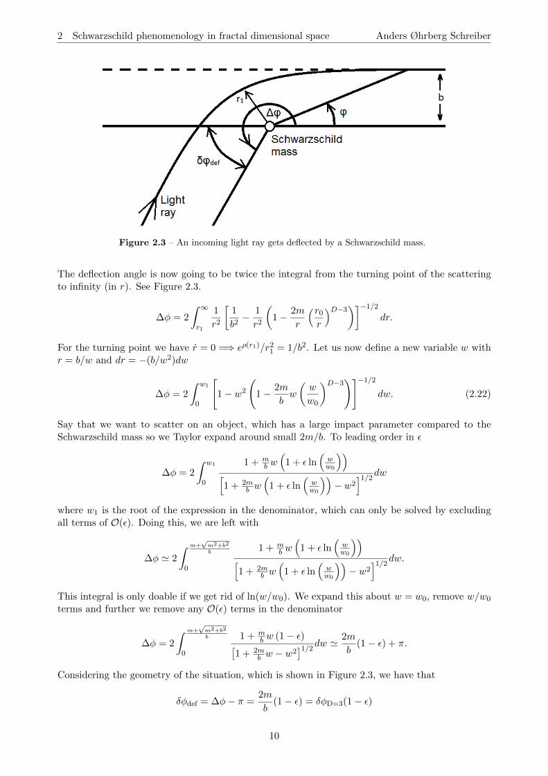
Figure 2.3 – An incoming light ray gets deflected by a Schwarzschild mass.

The deflection angle is now going to be twice the integral from the turning point of the scatteringto infinity (in r). See Figure 2.3.

∆φ = 2

∫ ∞r1

1

r2

[1

b2− 1

r2

(1− 2m

r

(r0

r

)D−3)]−1/2

dr.

For the turning point we have r = 0 =⇒ eρ(r1)/r21 = 1/b2. Let us now define a new variable w with

r = b/w and dr = −(b/w2)dw

∆φ = 2

∫ w1

0

[1− w2

(1− 2m

bw

(w

w0

)D−3)]−1/2

dw. (2.22)

Say that we want to scatter on an object, which has a large impact parameter compared to theSchwarzschild mass so we Taylor expand around small 2m/b. To leading order in ε

∆φ = 2

∫ w1

0

1 + mb w(

1 + ε ln(ww0

))[1 + 2m

b w(

1 + ε ln(ww0

))− w2

]1/2dw

where w1 is the root of the expression in the denominator, which can only be solved by excludingall terms of O(ε). Doing this, we are left with

∆φ ' 2

∫ m+√m2+b2

b

0

1 + mb w(

1 + ε ln(ww0

))[1 + 2m

b w(

1 + ε ln(ww0

))− w2

]1/2dw.

This integral is only doable if we get rid of ln(w/w0). We expand this about w = w0, remove w/w0

terms and further we remove any O(ε) terms in the denominator

∆φ = 2

∫ m+√m2+b2

b

0

1 + mb w (1− ε)[

1 + 2mb w − w2

]1/2dw ' 2m

b(1− ε) + π.

Considering the geometry of the situation, which is shown in Figure 2.3, we have that

δφdef = ∆φ− π =2m

b(1− ε) = δφD=3(1− ε)

10


which is the quantity usually considered when considering the bending of light in general relativity[11]. We thus get an expression for the bound on ε

|ε| <∣∣∣∣1− δφexp

δφD=3

∣∣∣∣which, when compared to perihelion precession, does not yield a very good bound, since the peri-

helion precession bound is supressed further by a factor of∣∣∣∆φperihelionπ

∣∣∣ � 1. We will therefore not

go into dataanalysis as outlooks for better bounds are not good.

2.4 Gravitional redshift

The last exploration we will do in the Schwarzschild metric is of gravitational redshifts. We willonce again see how well we can set bounds on ε with measurements of gravitational redshift andjudge if bounds have prospects of being good. To derive the formula for gravitational redshift, wewill follow the standard textbook method [11]. First consider the energy of a photon measured byan observer with velocity uµobs:

E = ~ω = −pµuµobs.

For a stationary timelike observer, the spatial components of uµobs are zero, so

g00u0obsu

0obs = −

(1− 2m

r

(r0

r

)D−3)u0

obsu0obs = −1⇐⇒ u0

obs =

(1− 2m

r

(r0

r

)D−3)−1/2

.

Since the metric (2.1) is static, the time direction must be a Killing direction (this can also be seensince ξµ

dxµ

ds = constant for a ξµ being a Killing vector), so uµobs ∝ ξµ. For a stationary observer atr = R, we have

~ωR = −(

1− 2m

R

(r0

R

)D−3)−1/2

(pµξµ)R

where the inner product is evaluated at R. Likewise for r → ∞ we have ~ω∞ = −(pµξµ)∞. Since

ξµ is a Killing vector pµξµ must be conserved along the geodesic of the photon. Thus to leading

order in ε we have

ω∞ '

(1− 2m

R

)1/2

− ε m ln(r0R

)R√

1− 2mR

ωR =⇒ |ε| ≤

∣∣∣∣∣∣R√

1− 2GmR

Gm ln(r0R

) [zD=3 − zobs]

∣∣∣∣∣∣where we have used that z = ω∞

ωR− 1 [4]. There is a problem with this bound, since we have the

free parameter, r0, stemming from our solution to the Schwarzschild metric. The presence of thisparameter makes us able to adjust the bound on ε indefinitely, as we can make ε very large byletting r0 → 1 in appropriate units and very small by letting r0 → ±∞. Thus gravitational redshiftis non-ideal for setting bounds on ε.

11

3 Hydrogen-like atoms in fractal and compactified space Anders Øhrberg Schreiber

3 Hydrogen-like atoms in fractal and compactified space

In this section we consider the effects of a fractal dimensional space and a compactified space inthe context of the quantum mechanical model for hydrogen-like atoms. First we solve the thissystem using the Schrodinger equation in D dimensions and compare the spectrum of this model toexperimental measurements to set bounds on the dimensional deviation from three dimensions.

Next up we consider an extension to the usual hydrogen-like model in the form of a compactifiedextra dimension. Initially we consider the Coulomb potential of the problem living only in the usualthree dimensions and of the form V (r) ∼ 1/r. Using this model, we derive the new spectrum forhydrogen and compare this to known experimental data. Lastly we consider what happens to thespectrum when the potential is also living in the compactified dimension.

3.1 Fractal dimensional space

We are going to model a hydrogen-like atom using nonrelativistic quantum mechanics. The standardway of modelling this problem is through the time-independent Schrodinger equation

Hψ = Eψ, (3.1)

which in general can be solved as both a differential equation and an eigenvalue problem. To specifya system in quantum mechanics, all we need is to provide the interactions of the system, which fora hydrogen-like atom is the Coulomb potential. Through scattering experiments it can be shownthat the Coulomb potential will go as 1/r at atomic scales [12]. Specifically we take the Coulombpotential to have the form

V (⇀r) = − Ze

2

4πε0

1

r≡ α

r(3.2)

where Z is the number of charged nucleons for the hydrogen-like atom. In the Schrodinger equationwe also have the kinetic energy part of the Hamiltonian operator and we want to determine the formof this in D dimensions. The kinetic energy operator goes as p2 and from first quantization this goesas the Laplacian operator. The Laplacian can be written in D dimensions in general curvilinearcoordinates [13]

∇2 =1

h

D−1∑i=0

∂

∂θi

(h

h2i

∂

∂θi

)

where θ0 ≡ r (the radial coordinate), h =∏D−1j=0 hj and h2

i =∑D

j=1

(∂xj∂θi

)2and xi are Cartesian

coordinates. In D dimensions, we define coordinate transformation between Cartesian coordinatesand spherical coordinates (see Appendix C). Using the transformations, the hj functions are

h0 = 1

h1 = r sin θ2 sin θ3 · · · sin θD−1

...

hj = r sin θj+1 sin θj+2 · · · sin θD−1

...

hN−1 = r

12


which results in the following Laplacian

∇2 =1

rD−1

∂

∂r

(rD−1 ∂

∂r

)+

1

r2

D−2∑i=1

1∏D−1j=i+1 sin2 θj

[1

sini−1 θi

∂

∂θi

(sini−1 θi

∂

∂θi

)]+

1

r2

[1

sinD−2 θD−1

∂

∂θD−1

(sinD−2 θD−1

∂

∂θD−1

)]. (3.3)

Defining angular momentum operators (see Appendix C) and combining these with the Laplacian,we get the full Hamiltonian operator for the problem

H = − ~2

2m∇2 + V (

⇀r) = − ~2

2m

[1

rD−1

∂

∂r

(rD−1 ∂

∂r

)− L2

D−1

r2

]+ V (

⇀r).

Now that we have the full Hamiltonian, we turn our attention to (3.1) and solving this. Seperatingvariables in the wavefunction, the radial Schrodinger equation reads

∂2R

∂r2+D − 1

r

∂R

∂r+

(2mE

~2− 2m

~2V (r)− l(l +D − 2)

r2

)R = 0. (3.4)

To ease solving this equation, we introduce the following definitions

r′ ≡ r

r0,

2mE

~2≡ − 1

4r20

, α′ ≡ 2mα

~2r0, R ≡ e−(1/2)r′

(r′)γf(r′) (3.5)

where α is defined from (3.2). We also define a potential in these coordinates

2m

~2V (r′)r2

0 ≡ −α′

r′. (3.6)

We get an equation for f(r′), by substituting (3.5) into (3.4) (see Appendix C)

r′∂2f

∂r′2+(2γ +D − 1− r′

) ∂f∂r′

+

(γ(γ +D − 2)− l(l +D − 2)

r′− 2γ +D − 1

2+ α′

)f = 0. (3.7)

We want the term ∼ 1/r′ to vanish to get a solveable equation. To make this term vanish we havetwo possible solutions for γ

γ+ = l (3.8)

γ− = −(l +D − 2). (3.9)

Using either of these solutions, (3.7) becomes

r′∂2f

∂r′2+(ϑ− r′

) ∂f∂r′− βf = 0 (3.10)

where ϑ = ±(2l + D − 1) and β = ±(

2l+D−12

)− α′. This is exactly a confluent hypergeometrical

differential equation, which has a solution of the form of a Kummer’s function [14]

f(ϑ, β, r′) =∞∑ν=0

(β + ν)!ϑ!

(ϑ+ ν)!β!

(r′)ν

ν!.

Since the factorial of negative integers are infinite and we want terms in the sum to be finite, weimpose

ϑ 6= −1,−2,−3, . . .

13


which means we have to omit the negative solution γ− (since negative ϑ come from the γ− solution).

Also, if the sum does not terminate, it will diverge faster than e12r′ for large r′ and such solutions

will not be normalizable. We therefore want to terminate the sum by letting β ∈ Z−. Since we usethe γ+ solution, we have the condition for termination on β

β = l +D − 1

2− α′ = −k, k ∈ N.

Since α′ is related to the eigenenergy through r0, we can now write an expression for the energyquantization

l +D − 1

2− 2mα

~2

√− ~2

8mE= −k ⇐⇒ E = −mα

2

2~2

1[l + D−1

2 + k]2 ≡ RD 1

n2

where RD is the Rydberg constant with subscript D to note that this might change in some non-trivial way with the number of spatial dimensions. The principal quantum number now becomesnon-integer

n =D − 1

2,D − 1

2+ 1,

D − 1

2+ 2, . . . . (3.11)

Putting back in α ≡ − Ze2

4πε0, we get

En = − m

2~2

(Ze2

4πε0

)21

n2(3.12)

which is in accordance with [15] for D = 3. Now we want to measure the dimension of space. Sincethe Rydberg constant in (3.12) might depend non-trivially on D, we look at the ratio of energydifferences to avoid this ambiguity

ξ(n) =En+2 − EnEn+1 − En

=∆En+2,n

∆En+1,n=λn+1,n

λn+2,n=

4(1 + n)3

(n+ 2)2(1 + 2n)(3.13)

where λn+1,n is the wavelength of a photon required to excite an electron from state n to n + 1.This is a tool for measuring the dimension of space from spectal data for hydrogen-like atoms, usingequation (3.11) and (3.13).

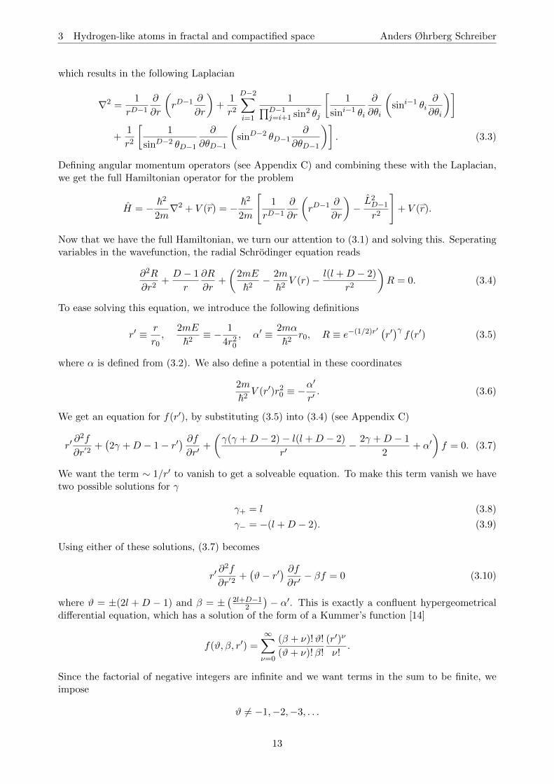
We want to use the above tools to set a bound on the size of the fractal dimension of space withD = 3 + ε. We can use (3.13) with spectral data on wavelengths for transitions in hydrogen [16] tofind measurements of the principal quantum numbers. From there we will use (3.11) to set boundson ε. Such calculations have been done and the ε bounds are shown in Figure 3.4. We find a meanε bound to be

|ε| ≤ (4.0± 2.3) · 10−4

which is at first sight inconsistent with ε = 0. One thing to consider here, like for the perihelionprecession data, is that the distribution in Figure 3.4 is not Gaussian. The distribution is stronglypeaked at zero and is one-sided. Therefore we cannot trust the mean and uncertainty of the mean,because these assume a Gaussian distribution around the mean.

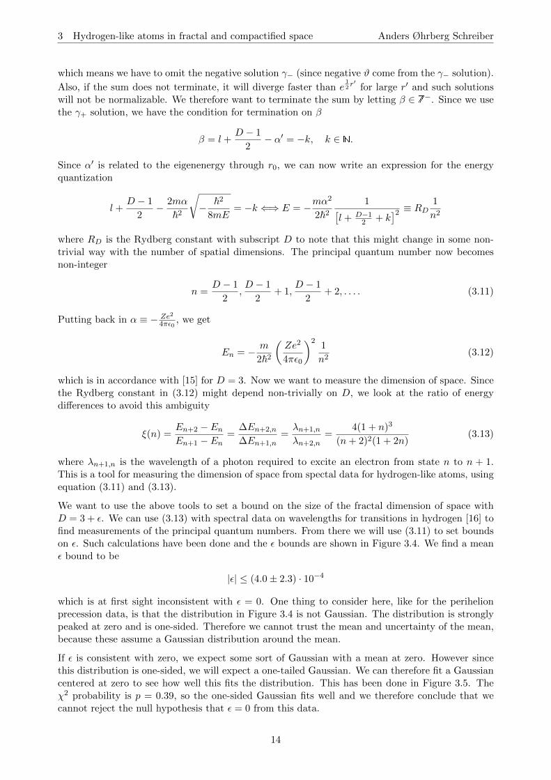
If ε is consistent with zero, we expect some sort of Gaussian with a mean at zero. However sincethis distribution is one-sided, we will expect a one-tailed Gaussian. We can therefore fit a Gaussiancentered at zero to see how well this fits the distribution. This has been done in Figure 3.5. Theχ2 probability is p = 0.39, so the one-sided Gaussian fits well and we therefore conclude that wecannot reject the null hypothesis that ε = 0 from this data.

14


Entries 10

Mean 0.0003935

RMS 0.0007284

Epsilon0 0.0005 0.001 0.0015 0.002 0.0025

Fre

quen

cy

0

1

2

3

4

5

6Entries 10

Mean 0.0003935

RMS 0.0007284

Figure 3.4 – The distribution of ε bounds from [16].

Entries 10

Mean 0.0003935

RMS 0.0007284

/ ndf 2χ 3 / 3

Prob 0.3917


Width 6.151e-009± 1.018e-008

Epsilon0 0.0005 0.001 0.0015 0.002 0.0025

Fre

quen

cy

0

1

2

3

4

5

6

Entries 10

Mean 0.0003935

RMS 0.0007284

/ ndf 2χ 3 / 3

Prob 0.3917


Width 6.151e-009± 1.018e-008

Figure 3.5 – A χ2 fit of a positive Gaussian centered at zero to our distributionof ε bounds. The χ2 probability is good so we can trust the fit.

3.2 Compactification on S1: V (r) ∼ 1/r ∈ R3

We now turn our attention to the case where we have four dimensions, but with one dimensionsbeing subject to compactification. We impose that the Coulomb potential of the problem lives onlyin three of the four dimensions so those three dimensions will be described by spherical coordinatesdue to the inherent spherical symmetry of the potential. To achieve compactification of the fourthdimension, we impose the identification w ∼ w + 2π [1], so that the fourth dimension is describedwith an angular coordinate w and a radius R. The Laplacian takes the form

∇2D=4 =

1

r2

∂

∂r

(r2 ∂

∂r

)+

1

r2 sin θ

∂

∂θ

(sin θ

∂

∂θ

)+

1

r2 sin2 θ

∂2

∂φ2+

1

R2

∂2

∂w2.

15


Therefore we get the Hamiltonian

H =

[− ~2

2m∇2 + V (r)

]− ~2

2mR2

∂2

∂w2. (3.14)

Seperating variables yields a function split ψ(r, θ, φ, w) = ψ(r, θ, φ)ϕ(w), which gives us the time-independent Schrodinger equation

1

ψ(r, θ, φ)

[− ~2

2m∇2 + V (r)

]D=3

ψ(r, θ, φ)− 1

ϕ(w)

~2

2mR2

∂2

∂w2ϕ(w) = ED=3 + Ew.

The (r, θ, φ) part will lead to the usual hydrogen-like solution [15]. Due to the identification on w,we get a periodic boundary condition on ϕ(w), which leads to the solution

ϕk(w) = ak sin (kw) + bk cos (kw) (3.15)

where k ∈ Z. The total eigenenergy associated with ψnlm(r, θ, φ) and ϕk(w) is therefore

En,k = − m

2~2

(Ze2

4πε0

)21

n2+

~2

2m

(k

R

)2

.

So there is a correction to the energy levels. We know that in D = 3 case, n = 1, 2, . . ., so here n = 1is the groundstate here. For the new correction, we can have k = 0,±1,±2, . . .. The groundstatehere is k = 0, but this yields no correction and is not interesting. The first excitation in k is k = ±1.

To set upper bounds on the size of the extra dimensions, we will work under the assumption thatit is harder to excite an electron in the extra dimension than it is to ionize hydrogen-like atoms.Excitations in the extra dimension will therefore not be seen (and this is indeed what we expect).For hydrogen (Z = 1) we get the following bound on R

m

2~2

(e2

4πε0

)2

<~2

2m

1

R2⇐⇒ R <

~2

m

(e2

4πε0

)−1

= 5.30 · 10−11 m.

This length scale cannot be probed by gravity yet, where the current best upper bounds are [17]R < 0.16 · 10−9 m. This is however for two flat extra dimensions of equal size, meaning that we geta contribution from each of the two dimensions. Assuming two extra dimensions instead of one, ourcalculation will simply change by a factor

√2 on the upper bound on R. We thus set a contraint

on the size of two extra dimensions from hydrogen

Rtwo compact dim., hydrogen < 7.48 · 10−11 m.

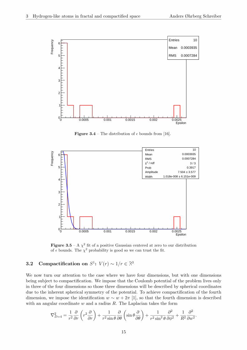
We can also use data [16] for heavier hydrogen-like atoms to set even better upper bounds on R.This can be seen in Figure 3.6. We see that the larger the ionization energy, the smaller the upperbound. The best upper bound is achieved, in this dataset, through the hydrogen-like atom of atomicnumber 110 (darmstadtium)

Rtwo compact dim., darmstadtium < 6.11 · 10−13 m.

Thus we have improved the bound on the radius of two extra dimensions (through electric interac-tions) by 3 orders of magnitude when comparing to [17]. However, as upper bounds of R goes as1/Z2, Z being the proton number of the nuclei, we could in principle get upper bounds on R going tozero for Z →∞. However we might hit a stability limit as nuclei become larger and larger in orderto contain the enormous amount of protons. To date we have produced up to atomic number 118and this might be near an upper limit. If however there could exist stable nuclei with an arbitrarynumber of protons, we could get arbitrarily small upper bounds on R. To see if this is possible wehave to delve into nuclear physics which will be beyond the scope of this thesis.

16


Atomic number0 20 40 60 80 100 120

Rad

ial u

pper

bou

nd [m

]

0

10

20

30

40

50

60

70

80

-1210×Radial upper bounds for two extra dimensions of equal radius

Figure 3.6 – Radial upper bounds on two compact extra dimensions of equalradius from ionization data of hydrogen like atoms [16]. We see a clear tendencyfor the data and indeed R bounds should go as 1/Z2 (Z being the atomicnumber).

3.3 Changing the potential domain: V (r) ∼ 1/r ∈ R3 × S1

In this last part we will work out what happens if we change the potential after we add a compactifiedextra dimension. We have so far assumed that the potential goes as ∼ 1/r, with r being the usualradial coordinate in three dimensions. We will now consider what happens if the Coulomb potentiallives in all four dimensions. The potential takes the form

V (⇀r) = − Ze

2

4πε0

(1√

r2 +R2w2

).

Taking now that the volume of the dimension is small, we expand to leading order in R

V (⇀r) = − Ze

2

4πε0

[1

r− w2R2

2r3

].

We can now see that for small R, the second term in the expanded potential can be seen as aperturbation

H ′ = R2 Ze2

4πε0

w2

2r3.

Taking the known solution to hydrogen-like atoms in three dimensions [15] and equation (3.15),we can calculate the contribution of this pertubation to first order in the usual time-independentpertubation theory [15] for the groundstate (n = 1, k = 0)

E(1)1,0 = 〈ψ1,0|H ′|ψ1,0〉 .

For k = 0, the wavefunction in the extra dimension is simply ϕ0(w) = b0, so the w integral from

the first order perturbation is 〈ψ1,0|H ′|ψ1,0〉w ∝(2π)3

3 . Using the groundstate wavefunction for

hydrogen-like atoms [15], ψ100(r, θ, φ) = Z3/2√πa3

e−Zr/a, where a is the Bohr radius, the expectation

17


−→

2πR

2πR

re

p

Image

Image

Image

Image

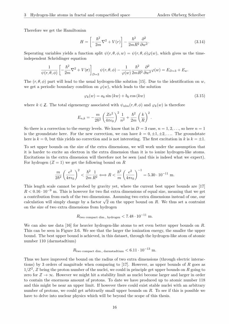
Figure 3.7 – Images of the proton by unfolding the extra dimension.

value of 1/r3 is divergent, so the only way to resolve this is to remove the perturbation, i.e. letR → 0. This also makes it impossible to get an excitation in the extra dimension as the energyeigenvalue in the unperturbed problem is infinite for l 6= 0. Thus we have removed the extradimension.

One could also consider a potential ∼ 1/r2 with a compactified dimension [18] as this is motivatedfrom the solution to the Poisson equation for a point charge in four dimensions. One can then usethe method of images to find the potential between the electron and proton, since the periodicityof the extra dimension implies an infinite set of proton images that contribute to the potential. SeeFigure 3.7.

Vcompact(⇀r) =

1

4π2

∞∑n=−∞

e2

r2 + (w − 2πnR)2.

Using complex analysis, it is possible to sum up this expression to (see Appendix D)

Vcompact(⇀r) = − e2

8π2Rr

sinh(r/R)

cosh(r/R)− cos(w/R).

There is also a second part to the potential, which is the interaction between the electron and itsimages, but this is simply a constant [18]. One can show, using the standard variational principle[15, ?], that it is possible to have an unbounded groundstate energy [18]. This result also holds truefor large extra dimensions. This implies that the atoms, if the potential was of the form ∼ 1/r2

would not be stable. Since we however do have stable atoms in nature, we will reject this kind ofpotential as physical.

18

4 Summary and outlook Anders Øhrberg Schreiber

4 Summary and outlook

In this thesis we have developed a formalism for setting a fractal dimensional bound on the deviationfrom three spatial dimensions, ε, as well as setting bounds on compactified extra dimensions of radiusR. This has been done specifically through the framework of general relativity and non-relativisticquantum mechanics.

We derived the Schwarzschild metric in D+1 dimensions and with that a formula for setting boundson ε through measurements of perihelion precession. From perihelion precession in binary pulsarsystems we conclude that ε = 0 is consistent with the measurements through fitting a one-sidedGaussian to the achieved distribution of ε bounds. We have also found that bending of light makesworse bounds on ε than perihelion precession and that gravitational redshift has an adjustableparameter making it impossible to get consistent bounds.

In quantum mechanics we derived a formalism for setting bounds on ε from hydrogen spectral data.Bounds on ε are indeed consistent with ε = 0.

For a fractal dimensional spacetime we conclude that we cannot reject the null hypothesis thatε = 0. The best upper bound on ε was found from perihelion precession in the binary neutron starsystem PSR J0737-3039A

|ε| ≤ 5.0 · 10−9.

We have looked at how to set bounds on the radius of compact extra dimensions. First with theCoulomb potential being present only in the three large dimensions, we have for two compactifiedextra dimensions of equal size R set an upper bound of

Rtwo compact dim., darmstadtium < 6.11 · 10−13 m.

We have also tried to include let the Coulomb potential live in the extra dimension. Perturbationtheory breaks down at first order for this case, and we therefore have to set R→ 0 and remove theextra dimension in order to fix this divergence. When using a potential of the form ∼ 1/r2, withone compact extra dimension, it is possible to have an unbounded (below) groundstate energy [18]and therefore electromagnetically stable atoms do not exist.

All attempts to confirm the presence of extra dimensions at the astrophysical and atomic level havefailed. The assumption of three spatial dimensions is therefore still good at the energy levels wehave been concerned with.

Acknowledgement

I would like to thank my advisor Emil Bjerrum-Bohr for having done a great job at directing mystudies during the work of this thesis.

I would also like to thank the NBIA Lounge and Coffee room for providing a fantastic academicenvironment during this work.

19

5 Appendix A: Christoffel symbols for the Schwarzschild metric Anders Øhrberg Schreiber

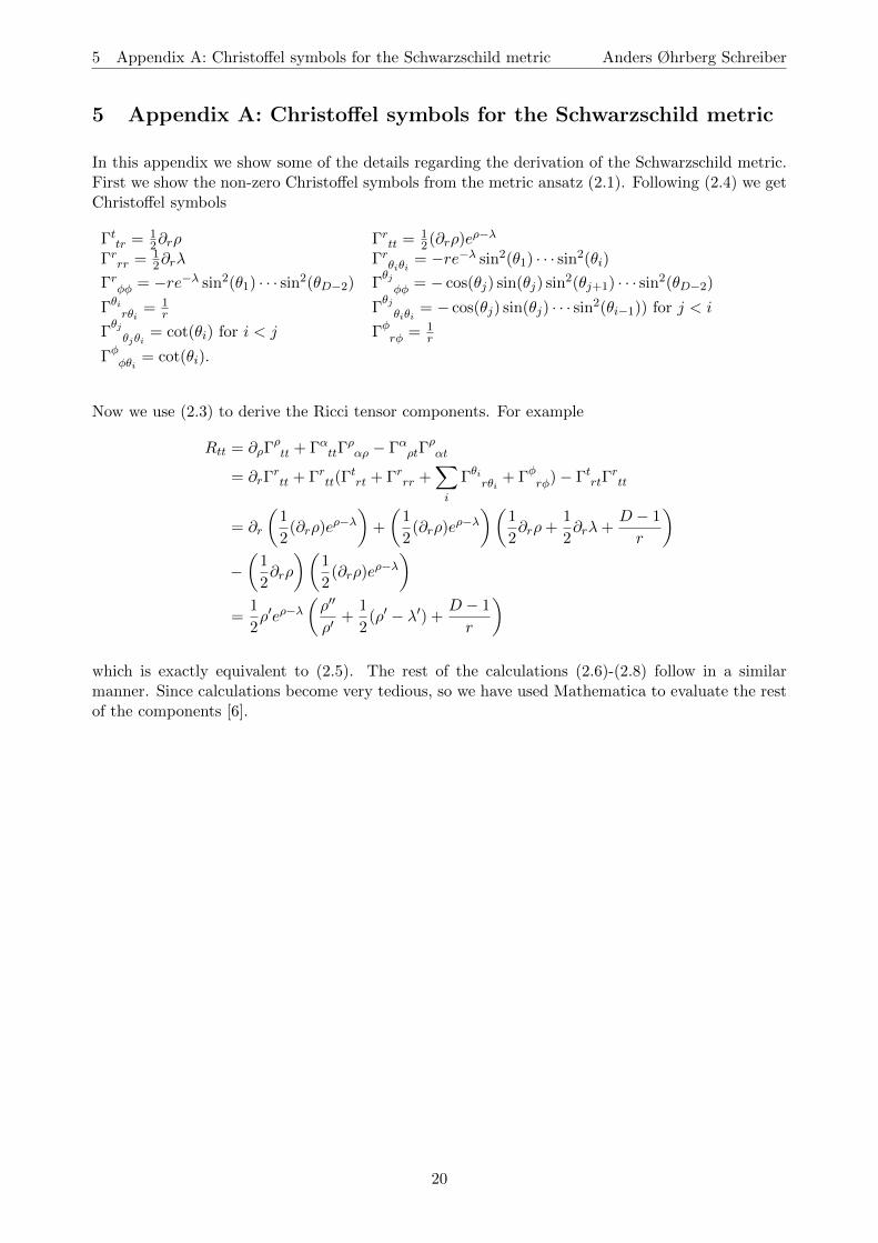
5 Appendix A: Christoffel symbols for the Schwarzschild metric

In this appendix we show some of the details regarding the derivation of the Schwarzschild metric.First we show the non-zero Christoffel symbols from the metric ansatz (2.1). Following (2.4) we getChristoffel symbols

Γttr = 12∂rρ Γrtt = 1

2(∂rρ)eρ−λ

Γrrr = 12∂rλ Γrθiθi = −re−λ sin2(θ1) · · · sin2(θi)

Γrφφ = −re−λ sin2(θ1) · · · sin2(θD−2) Γθjφφ = − cos(θj) sin(θj) sin2(θj+1) · · · sin2(θD−2)

Γθirθi = 1r Γ

θjθiθi

= − cos(θj) sin(θj) · · · sin2(θi−1)) for j < i

Γθjθjθi

= cot(θi) for i < j Γφrφ = 1r

Γφφθi = cot(θi).

Now we use (2.3) to derive the Ricci tensor components. For example

Rtt = ∂ρΓρtt + ΓαttΓ

ραρ − ΓαρtΓ

ραt

= ∂rΓrtt + Γrtt(Γ

trt + Γrrr +

∑i

Γθirθi + Γφrφ)− ΓtrtΓrtt

= ∂r

(1

2(∂rρ)eρ−λ

)+

(1

2(∂rρ)eρ−λ

)(1

2∂rρ+

1

2∂rλ+

D − 1

r

)−(

1

2∂rρ

)(1

2(∂rρ)eρ−λ

)=

1

2ρ′eρ−λ

(ρ′′

ρ′+

1

2(ρ′ − λ′) +

D − 1

r

)

which is exactly equivalent to (2.5). The rest of the calculations (2.6)-(2.8) follow in a similarmanner. Since calculations become very tedious, so we have used Mathematica to evaluate the restof the components [6].

20

6 Appendix B: Perihelion precession derivation steps Anders Øhrberg Schreiber

6 Appendix B: Perihelion precession derivation steps

In this appendix we fill in some of the details regarding the derivation of perihelion precession inD = 3 + ε dimensions. To get to equation (2.17), we first substitute into the Lagrangian, theintegrated equations of motion and the conditions on θi and θi, we get

k2e−ρ − e−ρr2 − h2

r2= 1. (6.1)

Let u = 1r . Then

r =dr

ds=

d

ds

(1

u

)= − 1

u2

(du

dφ

)(dφ

ds

)= − 1

u2hu2 du

dφ= −hdu

dφ.

Substituting this into (6.1), we get

k2e−ρ(u) − h2e−ρ(u)

(du

dφ

)2

− h2u2 = 1 ⇒ k2

h2+

(du

dφ

)2

− u2eρ(u) =eρ(u)

h2.

Introducing (2.9) into the above expression, we get

k2

h2−(du

dφ

)2

− u2

(1− 2mu

(u

u0

)D−3)

=1

h2

(1− 2mu

(u

u0

)D−3). (6.2)

Let D = 3 + ε, so (6.2) becomes

k2

h2−(du

dφ

)2

− u2

(1− 2mu

(u

u0

)ε)=

1

h2

(1− 2mu

(u

u0

)ε)⇔ (6.3)(

du

dφ

)2

+ u2 =k2

h2+

1

h22mu

(u

u0

)ε+ 2mu3

(u

u0

)ε. (6.4)

Taking the derivative with respect to φ and dividing by 2 gives

d2u

dφ2+ u =

1

h2m

(u

u0

)ε+

1

h2mε

u

u0

(u

u0

)ε−1

+ 3mu2

(u

u0

)ε+mε

u3

u0

(u

u0

)ε−1

⇔

d2u

dφ2+ u = (1 + ε)

m

h2

(u

u0

)ε+ (3 + ε)mu2

(u

u0

)εwhich is exactly (2.17).

Taking the part proportional to A in (2.18), we get

A =m

h2+ 3mA2 +O(ε).

Solving this equation for A gives

A =h2 ± h

√h2 − 12m2

6mh2.

Picking the negative solution, and expanding about m = 0 to third order, we get

A =m

h2+ 3

m3

h4+O(m4).

Taking the part proportional to B in (2.18), we get

1− ω2 ' ε+ (6 + 5ε)m2

h2+ 6ε

m2

h2ln

(A

u0

)where we have thrown away terms ∼ (m/h)4 terms away. Solving for ω we get

ω =

√1− 6

m2

h2− ε ' 1− 3

m2

h2− ε

2.

21

7 Appendix C: Derivatives in the radial Schrodinger equation Anders Øhrberg Schreiber

7 Appendix C: Derivatives in the radial Schrodinger equation

In this appendix we fill in some of the details regarding the derivation of the spectrum for hydrogen-like atoms in D dimensions with a Coulomb potential. The transformations between Cartesian andspherical coordinates in D dimensions are given by

x1 = r cos θ1 sin θ2 sin θ3 · · · sin θD−1

x2 = r sin θ1 sin θ2 sin θ3 · · · sin θD−1

...

xi = r cos θi−1 sin θi sin θi+1 · · · sin θD−1

...

xN = r cos θD−1

where 0 ≤ r <∞, 0 ≤ θ1 ≤ 2π, 0 ≤ θi ≤ π for 2 ≤ i ≤ D − 1, and r2 =∑D

j=1 x2j .

Angular momentum operators are defined, inspired by the form of the Laplacian

L21 ≡ ~2 ∂

2

∂θ21

L22 ≡ ~2

[1

sin θ2

∂

∂θ2

(sin θ2

∂

∂θ2

)− L1

2

sin2 θ2

]...

L2i ≡ ~2

[1

sini−1 θi

∂

∂θi

(sini−1 θi

∂

∂θi

)− L2

i−1

sin2 θi

]...

L2D−1 ≡ ~2

[1

sinD−2 θD−1

∂

∂θD−1

(sinD−2 θD−1

∂

∂θD−1

)− L2

D−2

sin2 θD−1

].

With substituting the variables in (3.5) and (3.6) into (3.4), we get

1

r20

∂2R

∂r′2+D − 1

r′r20

∂R

∂r′+

(− 1

4r20

+α′

r′r20

− l(l +D − 2)

r′2r20

)R = 0⇔

∂2R

∂r′2+D − 1

r′∂R

∂r′+

(−1

4+α′

r′− l(l +D − 2)

r′2

)R = 0. (7.1)

We now use (3.5), so

R = e−(1/2)r′(r′)γf(r′)

which gives derivatives of R with respect to r′

∂R

∂r′= −1

2e−

12r′(r′)γf(r′) + γe−

12r′(r′)γ−1f(r′) + e−

12r′(r′)γ

∂f(r′)

∂r′

∂2R

∂r′2=

1

4e−

12r′(r′)γf(r′)− γ

2e−

12r′(r′)γ−1f(r′)− 1

2e−

12r′(r′)γ

∂f(r′)

∂r′

− γ

2e−

12r′(r′)γ−1f(r′) + γ(γ − 1)e−

12r′(r′)γ−2f(r′) + γe−

12r′(r′)γ−1∂f(r′)

∂r′

− 1

2e−

12r′(r′)γ

∂f(r′)

∂r′+ γe−

12r′(r′)γ−1∂f(r′)

∂r′+ e−

12r′(r′)γ

∂2f(r′)

∂r′2

22

7 Appendix C: Derivatives in the radial Schrodinger equation Anders Øhrberg Schreiber

=1

4e−

12r′(r′)γf(r′)− γe− 1

2r′(r′)γ−1f(r′)− e− 1

2r′(r′)γ

∂f(r′)

∂r′+ γ(γ − 1)e−

12r′(r′)γ−2f(r′)

+ 2γe−12r′(r′)γ−1∂f(r′)

∂r′+ e−

12r′(r′)γ

∂2f(r′)

∂r′2.

If we insert these back into (7.1) and dividing through by e−12r′(r′)γ , we get

1

4f − γ

r′f − ∂f

∂r′+γ(γ − 1)

r′2f +

2γ

r′∂f

∂r′+∂2f

∂r′2+

(D − 1)

r′

(−1

2f +

γ

r′f +

∂f

∂r′

)+

(α′

r′− 1

4− l(l +D − 2)

r′2

)f = 0⇔

r′∂2f

∂r′2+ (−r′ + 2γ + (D − 1))

∂f

∂r′+

(−γ +

γ(γ − 1)

r′− (D − 1)

2+γ(D − 1)

r′+ α′ − l(l +D − 2)

r′

)f = 0⇔

r′∂2f

∂r′2+ (2γ +D − 1− r′) ∂f

∂r′+

(γ(γ +D − 2)− l(l +D − 2)

r′− 2γ +D − 1

2+ α′

)f = 0

which is exactly (3.7).

23

8 Appendix D: Evaluating the potential with the method of images Anders Øhrberg Schreiber

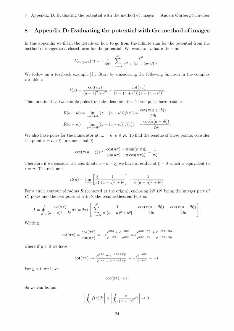
8 Appendix D: Evaluating the potential with the method of images

In this appendix we fill in the details on how to go from the infinite sum for the potential from themethod of images to a closed form for the potential. We want to evaluate the sum

Vcompact(r) = − 1

4π2

∞∑n=−∞

e2

r2 + (w − 2πnR)2.

We follow an a textbook example [?]. Start by considering the following function in the complexvariable z

f(z) =cot(πz)

(a− z)2 + b2=

cot(πz)

(z − (a+ ib))(z − (a− ib)) .

This function has two simple poles from the denominator. These poles have residues

R(a+ ib) = limz→a+ib

[(z − (a+ ib))f(z)] =cot(π(a+ ib))

2ib,

R(a− ib) = limz→a−ib

[(z − (a− ib))f(z)] = −cot(π(a− ib))2ib

.

We also have poles for the numerator at zn = n, n ∈ N. To find the residue of these points, considerthe point z = n+ ξ for some small ξ

cot(π(n+ ξ)) ' cos(nπ) + π sin(mπ)ξ

sin(nπ) + π cos(nπ)ξ=

1

πξ.

Therefore if we consider the coordinate z−n = ξ, we have a residue at ξ = 0 which is equivalent toz = n. The residue is

R(n) = limz→n

[ξ

πξ

1

(a− z)2 + b2

]=

1

π[(a− n)2 + b2].

For a circle contour of radius R (centered at the origin), enclosing 2N (N being the integer part ofR) poles and the two poles at a± ib, the residue theorem tells us

I =

∮C

cot(πz)

(a− z)2 + b2dz = 2πi

[N∑

n=−N

1

π[(a− n)2 + b2]+

cot(π(a+ ib))

2ib− cot(π(a− ib))

2ib

].

Writing

cot(πz) =cos(πz)

sin(πz)= −ie

iπz + e−iπz

e−iπz − eiπz = ieiπx−πy + e−iπx+πy

eiπx−πy − e−iπx+πy

where if y > 0 we have

cot(πz)→ ieiπx + e−iπx+πy

eiπx − e−iπx+πy∼ −ie

−iπx

e−iπx= −i.

For y < 0 we have

cot(πz)→ i.

So we can bound ∣∣∣∣∮Cf(z)dz

∣∣∣∣ ≤ ∣∣∣∣∮C

k

(a− z)2dz

∣∣∣∣→ 0.

24

8 Appendix D: Evaluating the potential with the method of images Anders Øhrberg Schreiber

This makes us able to write

∞∑n=−∞

1

(a− n)2 + b2=π

b

i[cot(π(a+ ib))− cot(π(a− ib))]2

=π

b

sinh(2πb)

cosh(2πb)− cos(2πa).

So going back to the potential, we have

Vcompact(r) = − 1

4π2(2πR)2

∞∑n=−∞

e2

r2

(2πR)2+(w

2πR − n)2 = − e2

8π2Rr

sinh(r/R)

cosh(r/R)− cos(w/R).

25

References Anders Øhrberg Schreiber

References

[1] B. Zwiebach, A First course in String Theory, Second Edition, Cambridge University Press,2009

[2] http://en.wikipedia.org/wiki/List_of_unsolved_problems_in_physics (Dec. 17, 2014)

[3] A. Schafer and B. Muller, Improved Bounds on the Dimension of Space-Time. Phys. Rev. Lett.,Vol 56, 12 (1986)

[4] R. M. Wald, General Relativity. University of Chicago Press, 1984

[5] A. Schafer and B. Muller, Bounds for the fractal dimension of space. J. Phys. A: Math. Gen. 19(1986) 3891-3902

[6] http://wps.aw.com/aw_hartle_gravity_1/7/2001/512494.cw/index.html (Jan. 7, 2015)

[7] S. Carroll, Spacetime and Geometry: An introduction to General Relativity. Pearson Eduction,inc., 2004.

[8] M. Kramer et al., Tests of General Relativity from Timing the Double Pulsar. Science 314, 97(2006).

[9] Australia Telescope National Facility, Pulsar Catalog. Catalog Version 1.50.

[10] Dyson, F. W., Eddington, A. S., Davidson C. (1920). ”A determination of the deflection of lightby the Sun’s gravitational field, from observations made at the total eclipse of 29 May 1919”.Philosophical Transactions of the Royal Society 220A: 291–333.

[11] J. Hartle, Gravity: An Introduction to Einstein’s General Relativity. Pearson Education, inc.,2003.

[12] F. Burgbacher et al., J. Math. Phys. 40 2, 625 (1999).

[13] N. E. J. Bjerrum-Bohr, J. Math. Phys. 41 5, 2515 (2000).

[14] F. W. J. Olver, D. W Lozier, R. F. Boisvert, C. W. Clark, Nist Handbook of MathematicalFunctions University Press, Cambridge, 2010.

[15] D. J. Griffiths, Introduction to Quantum Mechanics Pearson Education Inc., Peason PrenticeHall, 2005.

[16] Kramida, A., Ralchenko, Yu., Reader, J., and NIST ASD Team (2014). NIST Atomic SpectraDatabase (ver. 5.2).

[17] K.A. Olive et al. (Particle Data Group), Chin. Phys. C, 38, 090001 (2014).

[18] M. Bures, Atoms In Compactified Universes. Master’s Thesis, Masaryk University Brno, May2007. http://is.muni.cz/th/52540/prif_m/diplomka.pdf.

26

http://en.wikipedia.org/wiki/List_of_unsolved_problems_in_physics

http://wps.aw.com/aw_hartle_gravity_1/7/2001/512494.cw/index.html

http://is.muni.cz/th/52540/prif_m/diplomka.pdf

AndersSchreiber_ThesisFinal

Documents

dimension of space

fractal dimensional

upper bounds

appendix c

appendix d

dimensionality of space

d spatial dimensions

better bounds