Monitoring, Evaluation and Technical Support Services (USAID‐ METSS) Research Portfolio: 2014 ‐ 2015 Vincent Amanor‐Boadu, Professor, Agribusiness Economics and Management Kara Ross, Research Assistant Professor Yacob Zereyesus, Research Assistant Professor Aleksan Shanoyan, Assistant Professor Frank Kyekyeku, Doctoral Candidate, Agribusiness and Agricultural Economics Elizabeth Gutierrez, MS Student Agness Mzyece, MS Student and Fulbright Scholar Department of Agricultural Economics Kansas State University, Manhattan, KS 66506 October 2015

Welcome message from author
This document is posted to help you gain knowledge. Please leave a comment to let me know what you think about it! Share it to your friends and learn new things together.
Transcript

Monitoring, Evaluation and Technical Support Services (USAID‐METSS)
Research Portfolio: 2014‐2015
Vincent Amanor‐Boadu, Professor, Agribusiness Economics and Management
Kara Ross, Research Assistant Professor
Yacob Zereyesus, Research Assistant Professor
Aleksan Shanoyan, Assistant Professor
Frank Kyekyeku, Doctoral Candidate, Agribusiness and Agricultural Economics
Elizabeth Gutierrez, MS Student
Agness Mzyece, MS Student and Fulbright Scholar
Department of Agricultural Economics
Kansas State University, Manhattan, KS 66506
October 2015


Contents
Macroeconomic Effects on Poverty Rate: A Case Study of Northern Ghana ............................................... 1
Income, Expenditure Shares, Food Choices and Food Security in Northern Ghana ................................... 16
Do Adult Equivalence Scales Matter in Poverty Estimates? A Case Study from Ghana ............................. 23
A Cautionary Note on Comparing Poverty Prevalence Rates ..................................................................... 43
Securing Africa’s Middle Class: The Case of Northern Ghana .................................................................... 53
The Effect of Transaction Costs on Grain and Oilseed Farmers’ Market Participation in Sub‐Saharan
Africa: Recent Evidence from Northern Ghana ......................................................................................... 64
Reducing Gender Differences in Agricultural Performance in Northern Ghana ........................................ 82
Production Efficiency of Smallholder Farms in Northern Ghana ................................................................ 99
Does Women’s Empowerment in Agriculture Matter in Children’s Health Status? Insights from Northern
Ghana ........................................................................................................................................................ 115
Recent Evidence of Health Effects of Women Empowerment: A Case Study of Northern Ghana ........... 130

1
Macroeconomic Effects on Poverty Rate: A Case Study of Northern
Ghana
Yacob Zereyesus and Vincent Amanor‐Boadu
Department of Agricultural Economics
Kansas State University
March 2015
Introduction
The prevalence of extreme poverty is externally determined by the established poverty line. In recent
years, it has been based on a daily per capita expenditure of $1.25, measured in 2005 Purchasing Power
Parity (PPP). Using PPP aims to eliminate the effect of exchange rates.
PPP is based on the Law of One Price – in the absence of transaction costs and trade barriers, identical
traded goods will have the same price in all markets when the prices are denominated in the same
currency. This implies that in the presence of transaction costs and trade barriers, identical traded
goods do not have the same price in all markets.
PPP is calculated in three stages:
Product stage: Estimation of the relative prices for individual goods and services
Product group stage: Estimation of relative prices for products in the same group, often an
average of the PPP for each of the products in the group
Aggregation level: Weighted averages of the PPP of the product groups where weights are the
expenditures on the product groups as established in national accounts
The basket of goods used in the estimation of the PPP is a sample of goods and services used in the
estimation of GDP. Final list is approximately 3,000 consumer goods and services, 30 government
occupations, 200 equipment and 15 construction projects. They also often generate a significant portion
of their domestic public revenues through imposed barriers to trade such as tariffs.
From the foregoing, the prevalence of poverty may be influenced by the changes in the prices of goods
in a country’s basket of goods when the assumption of zero transaction costs and absence of trade
barriers fail to hold. Most developing countries experience significant transaction costs in traded goods
because of their dependence on imports. The extent of the violation of the law of one price is

2
exacerbated by the proportion of consumption that is imported and changing foreign exchange situation
in the country.
Research Question
To what extent do macroeconomic conditions in a developing country influence the prevalence of
poverty? The macroeconomic conditions of interest are exchange rates and inflation, measured by the
consumer price index (CPI). For simplicity purposes, the research question ignores the non‐trivial effect
of population growth on the prevalence of poverty.
The question is important because the performance of intervention projects aimed at reducing poverty
may be adversely affected by inimical macroeconomic conditions over which the projects have no
control. Understanding and measuring the effect of these macroeconomic conditions allow project
managers to make the necessary adjustments to their achievements to help effectively monitor and
evaluate project performance.
Background
Suppose the perfect world where the real exchange rate is constant over time between two countries,
say U.S. and Ghana. Suppose also that a basket of goods produced in U.S. and Ghana were identical and
completely tradable. The law of one price would suggest that net of transportation costs, arbitrage
would insure that the dollar price of the basket is identical between Ghana and the U.S. – this is the
basic theory of PPP determination.
Let us begin with an illustration of the changing PPP measured as national currency per U.S. dollar in the
Euro Zone and the UK (Figure 1). Between 2009 and 2014, UK’s PPP has been increasing while the EU’s
has been declining. This implies that for people living in the UK needed a declining quantity of British
Pounds to purchase the same basket of goods as would be purchased in the U.S. for given price in U.S.
dollars while those living in the Euro Zone needed an increasing quantity of Euros. A declining PPP is,
therefore, an indicator of a worsening economic condition for residents in a particular country.
Let us define the real exchange rate, Q, as follows:
*Q SP P (1)
where S is the nominal exchange rate, P is the U.S. price level and P* is the price level in the country of
interest, say Ghana. When the real exchange rate is appreciating, it means the U.S. price of the bundle

3
of goods in the basket is increasing relative to the Ghanaian price. Now, when the real exchange rates
appreciates, then the real value of the dollar has depreciated, suggesting a decline in its purchasing
power, relatively speaking.
To get to know how Q affects the poverty level, it is necessary to try to understand the factors that
influence changes in Q. The real exchange rate between the currencies of the two countries may
change when there is a change in the relative demand for U.S. goods as a result of preference shift,
leading to total expenditure on U.S. goods increasing. The shift may arise from two principal sources.
An increase in global private and public demand for U.S. goods is one source of such shifts. This shift is
exacerbated when the relative increase in demand for U.S. goods is much higher than the increase in
demand for Ghana goods. In an increasingly interconnected world, imports tend to account increasing
share of development countries’ consumption. Another source of the shift is an increase in U.S.
Government expenditure on U.S. goods, an event that increases during recessionary periods in attempts
to boost demand as an economic stimulant. When these events shift the demand for U.S. goods,
equilibrium can only be restored if the relative price of U.S. goods vis‐à‐vis Ghana goods rose. From
Equation (1), this implies a decline in Q, i.e., the purchasing power of the U.S. dollar has increased
relative to the Ghana cedi. The corollary is true: that the purchasing power of the Ghana cedi has
declined and its purchasing power has fallen.

4
Figure 1: Purchasing Power Parities for UK and Euro Zone per US Dollar (2009‐2014)
Another source of change in the real exchange rate is a change in relative output supply in the U.S.
significantly exceeding that of Ghana. Output supply changes are a function of resource productivity‐
enhancing technologies, such as those for labor and capital. Tractors and other farm production
equipment are some of the visible productivity‐enhancing technologies that allow U.S. agriculture, for
example, to dwarf that of Ghana. One outcome of increasing productivity is increasing incomes and the
country with the highest relative productivity increase will also have the highest relative income
increase. Because the higher incomes often lead to increased consumption of imports, relative prices in
the U.S. need to fall to restore equilibrium. This fall in relative prices lead to an increase in Q and a fall
in the U.S. dollar in real terms. Conversely, Ghana’s relative productivity disadvantage suggests the
need for appreciation of the Ghana cedi in order to restore equilibrium, leading to an increase in
Ghana’s prices relative to those in the U.S., i.e., the Ghana cedi rises in real terms. The foregoing works
well if the goods and services in the basket of goods being compared between the two countries are all
traded. However, a fair proportion of goods in the basket of developing countries tend to be non‐
traded.
Purchasing Power Parity
0.765
0.770
0.775
0.780
0.785
0.790
0.795
0.800
0.63
0.64
0.65
0.66
0.67
0.68
0.69
0.7
0.71
2009 2010 2011 2012 2013 2014
Euro Zone PPP
UK PPP
UK Euro Zone

5
Equation (1) may be re‐specified to focus on the nominal exchange rate instead of the real exchange
rate because the real exchange rate is assumed fixed or constant over time. Thus, the nominal exchange
rate is:
*S QP P (2)
where Q Q when Q is constant over time. Equation (2) suggests that any changes in the national
price level will alter the exchange rate. The genius of PPP is that it determines the exchange rate merely
by the movement in relative prices. Given that Ghana’s inflation rate is higher than that of the U.S.,
exchange rate has to appreciate and the cedi will depreciate relative to the U.S. dollar, implying more
Ghana cedis are required to purchase a U.S. dollar.
Suppose we take the logs of both sides of Equation (2), using the lower‐case letters to represent a
variable’s log form, then we have:
*
t t ts q p p (3)
Taking the first differences in Equation (3), we get:
*1t t t t ts s s p p (4)
The story Equation (4) is telling is that the percentage in nominal exchange rate is equal to the
difference between the inflation rates in Ghana and the U.S. What we find here is that when price levels
are changing rapidly, i.e., the inflation rate is high, those rapidly changing price levels tend to dwarf
everything else, giving the PPP its effectiveness in explaining exchange rate movements.
However, in the short run, the PPP does not perform very well at all. Recognize that the PPP is based
essentially on trade and trade flows and a critical assumption that transaction costs and trade barriers
are zero. Yet, in the short run, tariffs and transportation costs are real barriers to trade that influence
the profitability of arbitrage opportunities. Again, because Ghana and the U.S. differ significantly in the
composition of their outputs, shifts in term of trade can cause Q to change. For example, being a net
importer of fertilizers, a positive shock on oil prices would affect Ghana’s productivity very differently
than the U.S., if we assume it to be a net exporter of fertilizers. More realistically, prices tend to be

6
sticky in the short run, causing the law of one price to fail to hold. This implies that changes in the
nominal exchange rate would also affect the real exchange rate.
What really challenges the PPP is the presence of non‐traded goods in the basket of goods because non‐
traded goods do not flow across national boundaries. Non‐traded goods include such items as firewood,
thatch roofing material, education and medical services, housing, etc. When the proportion of goods in
the basket are non‐traded, then the use of PPP becomes suspect.
Let us show the effect of non‐traded goods in the following model. Let P define the price index in Ghana
and α as the proportion of non‐traded goods in the basket of goods consumed in the country, then:
1n tP P P (5)
where the subscripts n and t refer to non‐traded and traded respectively. The real exchange rate may
now be represented as:
**
** * *(1 *) *
1
n
tn t t
n t tn
t
P
PP P PQ S S
P P PP
P
(6)
When Equation (6) is simplified, then we get:
**
**n
tt
t n
t
P
PPQ S
P P
P
(7)
Assuming the PPP holds for traded goods implies that the first part of Equation (7) equals one, which
implies that the real exchange rate is defined as follows:
**
*n
t
n
t
P
PQ
P
P
(8)

7
Equation (8) is saying that the real exchange rate will change if the relative price of non‐traded goods in
either countries changes. If we assume that the basket of goods in the U.S. has only traded goods, then
α =1, transforming Equation (8) to say that the real exchange rate changes with the relative price
changes between the traded and non‐traded goods in Ghana, i.e.:
**
*n
t
PQ
P
(9)
If we take the logs of Equation (9), then we can state that the real exchange rate in Ghana will
appreciate if the relative price of non‐traded goods to traded goods increases. That is:
* *n tq p p (10)
The Balassa‐Samuelson effect provides evidence that this is a common occurrence in explaining
differential economic growth. It argues that economic growth is associated more with increased
productivity in traded goods. When liberalization policies are being pursued, it is expected that the
price of non‐traded goods will rise relative to traded goods, leading to a rapid changes in the real
exchange rate. Indeed, it is the proportion of non‐traded goods in the basket of good consumed in
Ghana that allows the poverty line in Ghana to be so dramatically different from that in the U.S., say.
Effect of Exchange Rate on Poverty
From Equation (10), we noted that the larger the proportion of non‐traded goods in the basket of
consumed goods, the lower the rate of economic growth even when productivity in those non‐traded
goods increase. This is merely a result of the lack of arbitrage opportunities for those goods to exploit
the productivity gains.
Let us assess the potential effect of the exchange rate on the poverty level using consumption
expenditures given the foregoing analysis and using data collected from the study area in 2012 and are
described in Zereyesus et al. (2014).1 Consumption expenditures are defined to encompass
expenditures on four product categories: food; housing; durables; and non‐durables. Durables are
products lasting longer than a year, such as radios, bicycles and clothing. Non‐durables are defined by
1 Zereyesus, Y., K. Ross, V. Amanor-Boadu and T. Dalton. Baseline Feed the Future Indicators for Ghana,
2012, Manhattan, KS: Kansas State University Press, 2014.

8
elimination, i.e., they are all the goods that are not food, housing nor durables. They include education,
health care, beauty care and grooming services, firewood, roofing thatch, household fuel and
transportation. It is obvious that for the study location, the durable goods category have the most
traded goods while the other product categories comprise essentially non‐trade goods.
Consumption expenditure data in Ghana cedi were collected from about 4,410 households in the study
area. To present the average daily household per capita expenditure in U.S. dollar denominated PPP
2005( )PX required two variables: (a) the consumer price index (CPI); (b) the PPP conversion factor. Using
World Bank International Comparison Program’s estimates, the 2005 PPP conversion factor (ρ2005) was
determined to be 0.447. Bank of Ghana data indicated that Ghana’s CPI in 2005 (I2005) and in 2012 (I2012)
were respectively 183.7 and 412.4, with 2000 = 100. To convert the estimated average daily household
per capita expenditure in 2012 Ghana cedi into 2005 PPP, used the foregoing coefficients and the
following equation:
2012 2005 20122005 2012
2012 2005
183.70.9965
0.447*412.4
G GP GX I X
X XI
(11)
The proportion of individuals for whom 2005PX is less than $1.25 defines the poverty prevalence. Based
on the data collected in the study area, the foregoing approach yielded a poverty prevalence of 22.2
percent reported above for the study area. The question of interest in this research is this: What effect
do the changing exchange rates and inflation have on the estimated poverty rate? In other words,
based on the approach described in Equation (11), how would the poverty rate have been if the local
currency conversion rate (which we have shown to be influenced by the nominal exchange rate) and the
inflation rate prevailing today had been in place when the study was conducted? The more important
question is to what extent do these macroeconomic factors influence the performance of poverty
reduction intervention projects?
Before we begin our attempt to answer these questions, let us look at the changes that have been
occurring in the macroeconomic environment in Ghana. The daily market (nominal) exchange rate
between the GHS and the USD for June 2012 to December 2012 is presented in Figure 2. It shows that
the Ghana cedi was appreciating against the USD at an average daily rate of approximately 0.02 percent.

9
Figure 2: Daily Market Exchange Rate of the Ghana Cedi to the US Dollar (June 2012‐October 2014)
Data Source: Investing.com (http://www.investing.com/currencies/ghs‐usd‐historical‐data).
However, the trend reversed, as shown in Figure 3, with the cedi depreciating against the USD at an
approximate daily rate of 0.03 percent between November 2012 and July 2014. Indeed, Dzawu and
Brand (2014) noted that the Ghana cedi as the world’s worst‐performing currency against the U.S. dollar
in the first and second quarters of 2014.2 It is this reversal that presents significant adverse effect on
the poverty rate independent of what intervention project managers do, ceteris paribus.
The trends in the relative price ratio (see Equation (1) and Equation (2)), presented as the local current
unit rate and the consumer price index or inflation are presented in Figure 4. Unlike the exchange rate
which was depreciating against the U.S. dollar, both the local currency unit rate and the inflation rate
are increasing very rapidly. The correlation coefficients between the exchange rate and total inflation as
well as housing, food and beverage, transportation and non‐food inflation for January 2012 through
May 2014 were all high (above 84 percent), positive and statistically significant at the 1 percent level.
Energy prices, for example, are directly influenced by the exchange rate because petroleum products
are imported. Depreciating exchange rates increases the local cost of these products, which in turn
influence the cost of food, transportation, clothing and other goods and services in the consumer’s
basket. The increase in local cost of fuel, because of its ubiquitous effect on numerous segments of the
2 Dzawu, M.M. and R. Brand. World’s Worst Currency Drops as Ghana Pulls Back from IMF Aid, June 30,
2014, 9:03 AM. Available at http://www.bloomberg.com/news/2014-07-30/world-s-worst-currency-drops-as-ghana-pulls-back-from-imf-aid.html.
1.85
1.90
1.95
2.00
GHS:USD

10
economy, can even lead to increases in housing costs as rents are increased by property owners to
address their income effects resulting from inflationary pressures. For the CPI for all items in Ghana,
during the 2003 to 2012 period, the CPI had been increasing at an annual rate of 13.7 percent.
Regarding the LCU in Ghana and the international dollar conversion factor, the LCU has been
depreciating by an average of 17 percent annually during the 1990 to 2013 period. Historical data on
the LCU conversion rate show that the LCU in Ghana has been steadily declining in value in relation to
the international dollar (Figure 4). For example, using the private consumption conversion factors, one
international dollar was equivalent to 0.03 and 0.93 LCUs in 1990 and 2013, respectively (World Bank).
Figure 3: Daily Market Exchange Rate of the Ghana Cedi to the US Dollar (November 2012‐July 2014)
Data Source: Investing.com (http://www.investing.com/currencies/ghs‐usd‐historical‐data).
The foregoing graphs support the non‐independence between the nominal exchange rate and inflation.
The exchange rate elasticity of inflation is estimated as 0.49 (t‐value = 12.19; p > |t| = 0.00). This
suggests that a percentage change in exchange rate would result in about one‐half percent change in
the CPI. A critical observation is that the rapid inflation in Ghana during this period relative to that in
the U.S., for example, contributes to the exacerbating exchange rate trend.
Let us assume that people qualifying for the minimum wage in Ghana have a very low non‐traded goods
content in their consumption basket. This is because to be earning the minimum wage, the person is
probably living in an urban area and have some form of regulated employment. The effect of the
exchange rate depreciation on this group of people provides an illustration of how the depreciating
1.50
2.00
2.50
3.00
3.50
4.00
GHS:USD

11
exchange rate pulls down the overall consumption environment to exacerbate the risk of poverty. Figure
5 shows that the Government of Ghana over the past several years has responded to the changing U.S.
dollar exchange rate by increasing the minimum wage. However, the rapid depreciation of the Ghana
cedi in recent years has positioned the U.S. dollar equivalent of the minimum wage in April 2014 at
about the same level it was five years’ earlier, without the attendant effect of inflation discussed earlier.
If inflation is accounted for, then we would have a situation where the minimum wage is significantly
lower in its purchasing power equivalent in 2014 than it was in 2010. If we assume that people earning
minimum wage are the most vulnerable to economic vicissitudes, then it is plausible to conclude that
the depreciation of the GHS against the USD may be having some adverse effect on the poor.
Figure 4: Trends in the Local Currency Unit Rate and the Consumer Price Index
‐
0.10
0.20
0.30
0.40
0.50
0.60
0.70
0.80
0.90
1.00
0
50
100
150
200
250
300
350
400
450
2000 2001 2002 2003 2004 2005 2006 2007 2008 2009 2010 2011 2012 2013
LCU
CPI (2010=100)
CPI LCU

12
Figure 5: Minimum Daily Wage in Ghana Cedi and US Dollar Equivalent Using Market Exchange Rate
(January 2010‐April 2014)
Data Sources: Bank of Ghana (http://www.bog.gov.gh/) and Investing.com (http://www.investing.com/currencies/ghs‐usd‐
historical‐data).
Simulating the Effect of Exchange Rate and Inflation on the Poverty Rate
The paper, thus far, shows there is a direct link between the poverty rate and the macroeconomic
variables of inflation and exchange rate even when PPP is used because of the relatively high proportion
of non‐traded goods in the consumption basket of Ghanaians. This proportion of non‐traded goods in
the consumption basket is directly related to the risk of falling under the poverty line. That is, as
average daily per capita household expenditure decreases, the share of non‐traded goods in a
consumer’s basket increases. This is because, for example, they will be more likely to use firewood they
gathered from local forests than purchase charcoal for home energy needs, or water collected from
rainfall or a local ravine than purchase a tanker of water. We also noted the inability of PPP to perform
well in the short run when prices are sticky and transaction costs such as transportation costs which
directly influence prices cannot be arbitraged because of location and its effect on competition in the
provision of services. We showed the direct influence of the PPP and inflation on the poverty rate in
illustrating the approach used in measuring the poverty rate in Equation 11. We use this relationship to
explore the empirical effect of the local current unit rate and inflation on the poverty rate.
3.00
3.50
4.00
4.50
5.00
5.50
1.90
2.00
2.10
2.20
2.30
2.40
2.50
2.60
2.70
2.801‐Jan
‐10
1‐M
ar‐10
1‐M
ay‐10
1‐Jul‐10
1‐Sep
‐10
1‐Nov‐10
1‐Jan
‐11
1‐M
ar‐11
1‐M
ay‐11
1‐Jul‐11
1‐Sep
‐11
1‐Nov‐11
1‐Jan
‐12
1‐M
ar‐12
1‐M
ay‐12
1‐Jul‐12
1‐Sep
‐12
1‐Nov‐12
1‐Jan
‐13
1‐M
ar‐13
1‐M
ay‐13
1‐Jul‐13
1‐Sep
‐13
1‐Nov‐13
1‐Jan
‐14
1‐M
ar‐14
1‐M
ay‐14
Minim
um Daily W
ages (¢)
Minim
um Daily W
ages ($)
Min. Daily Wage (USD) Min. Daily Wage (GHS)

13
Figure 6 shows that keeping all things unchanged except the CPI, conducting the study today when the
estimated CPI is approximately 605.9 (2002 = 100) would lead to a poverty rate estimate of about 39
percent instead of the 22.2 percent estimated in 2012.3 The result is not very different when Ghana
Statistical Service’s CPI estimate of 141.1 (2012 = 100) for January 2015 is used after adjusting the base
year back to 2002.
Figure 6: Simulated CPI Effect on Poverty Rates
The relationship between the local currency unit rate and the poverty rate is defined in Equation (11).
Holding all variables constant, Figure 7 explores the effect of changing local currency unit on the poverty
rate. It shows that the local currency unit rate increases (i.e., the cedi weakens) in comparison to the
international dollar as we move from left to right on the horizontal‐axis. The red line superimposed on
the graph at the local currency unit rate value of 0.447 on the horizontal –axis shows the point we were
in 2012 when the poverty rate was 22.2 in the study area. With the current weakening of the cedi, if the
poverty rate was measured where the local currency unit rate is assumed to be 0.60, the estimated
poverty rate would be approximately 35 percent.
3 The estimated CPI assumed that the historical growth in the CPI between 2000 and 2013 will remain
unchanged. The applied formula is 414.2(1.137)3 =605.9.
0
5
10
15
20
25
30
35
40
45
50
55
60
65
70
1 101 201 301 401 501 601 701 801 901
Poverty Rate
CPI (2000 = 100)

14
Figure 7: Simulated Local Currency Unit Effect on Poverty Rates
Conclusion
The purpose of this paper was to understand the potential effect of changing macroeconomic conditions
on poverty even when PPP was the basis of measuring relative prices. We showed that in developing
countries that are experiencing rapid inflation and where the proportion of non‐traded goods in the
consumer goods basket is high in comparison to the U.S., PPP may fail to remain unchanging in the short
run. If such is the case, then it is plausible to recognize the potential effect of the relationships between
inflation and relative prices on the poverty rate.
We showed that Ghana has been experiencing rapid inflation since 2012 and the nominal exchange rate
has been rising rapidly. We showed that because of the relatively large proportion of non‐traded goods
in the consumption basket of the population in the study area, the relative price of non‐traded goods to
traded goods may be rising too. If that is the case, then the implied local currency unit rate would be
depreciating. The structure of the estimation procedure suggests that poverty rate would increase with
either of these events happening. This paper showed the empirical effect of the changes. We, however,
did not explore the interaction effect of both inflation and local currency unit rates increasing even
though that is exactly what is happening. However, the model shows that the combo effect the two
variables on the poverty rate is multiplicative, not additive.
0
5
10
15
20
25
30
35
40
45
50
55
60
65
70
75
80
85
0.00 0.10 0.20 0.30 0.40 0.50 0.60 0.70 0.80 0.90 1.00 1.10 1.20 1.30 1.40
Poverty Rate (%
)
Local Currency Unit (PPP Basis) (GHS/USD)

15
The Economic Growth Office has made investments in projects that are implementing programs to
ameliorate the estimated poverty level in the region and/or in the particular district of activity. The
projected target for poverty reduction is 20 percent. That is, the Economic Growth Office expects to
attain an average poverty rate of about 17.8 percent by the end of the project. This paper indicates that
the estimation method for conducting the evaluation of project objectives must be carefully structured
if the uncontrollable macroeconomic effects are going to be neutralized. It is critically important that
we construct an internal PPP that recognizes the specific macroeconomic conditions in the intervention
areas. This will help do two critical things in terms of reporting performance:
Understand the unique economic conditions under which the project participants are
operating, and hence appreciate the effect of those conditions on project performance; and
Develop a compelling explanation of any departures from targets which may not be the fault of
program managers, program designers or indeed have anything to do with the intervention
programs, period.
In this paper, we explored the effect of macroeconomic variables on attaining poverty reduction
program targets. We did not consider the demographic variable of population growth. As with the
macroeconomic variables, program evaluators must incorporate the changes in population in the
models develop to assess the performance of the projects. These uncontrollable variables are very
important in providing an accurate assessment of project performance and understanding the impact of
the intervention programs being implemented by the Economic Growth Office in Ghana.

16
Income, Expenditure Shares, Food Choices and Food Security in
Northern Ghana
Yacob A. Zereyesus, Vincent Amanor‐Boadu and Kara Ross
Department of Agricultural Economics
Kansas State University, Manhattan, KS 66506
January 2015
Introduction
Total expenditure is often used as a proxy in environments where income is difficult to measure
accurately. The relative ease of measuring household total expenditure, and from that the per capita
expenditure, underscores its inclusion as an indicator for monitoring and evaluating poverty and hunger
reduction programs. It is one of the central indicators of the Feed the Future initiative of the US
Government.
Higher incomes are associated with higher food security, allowing for a direct correlation assumption to
be made between higher total expenditures and improved food security and nutrition. Higher total
expenditures are also assumed to correlate indirectly with poverty risk. Understanding the distribution
of total household expenditure among the different categories of consumption could provide insights
into sources of vulnerability risks for policymakers and organizations seeking to ameliorate poverty in
poor countries. This paper presents information on the distribution of household expenditures among
consumpion categories in northern Ghana using data collected in 2012 for estimating baseline indicators
for USAID’s Feed the Future initiative in Ghana. The paper uses information from the expenditure
shares and incomes to assess the intensity of food security risks across income categories. It also assess
how food choices are influenced by income. The data covered 4,410 households and nearly 25,000
individuals across the area above Ghana’s Latitude 8˚N, covering only areas within Brong Ahafo,
Northern, Upper East and Upper West regions. The data used in this paper are available at US
Government Data.gov website (http://catalog.data.gov/dataset/feed‐the‐future‐ghana‐baseline‐
household‐survey).
Context of Consumption Expenditures
By definition of the study area, only a small portion of Brong Ahafo Region was covered in the survey,
with its represented population accounting for 12% of the survey’s respondents. Northern Region

17
accounted for 56% of respondents while Upper East and Upper West accounted for 18% and 13%
respectively. Overall, 51% of respondents were male while 78% of respondents lived in rural areas.
Nearly 85% of survey respondents had no formal education and only 12% had at most a secondary
education. The average household size across the study area was about six people. The average
prevalence of poverty across the study areas was estimated at about 22% using a poverty line of $1.25
daily per capita expenditure.
There are four main consumption categories: food; housing; durables; and non‐durables. Non‐durables
include such goods as fuel, transportation, education and health care, whether purchased, home
produced or received as gifts. Thus, harvested firewood is included in this category as are home‐
produced mats and beddings, school fees and health care costs. Durables include household items that
last more than a few years – refrigerators, radios, automobiles, bicycles, etc. Housing and food
categories are self‐explanatory. Housing expenditures are defined to include implicit valuation of
owned dwelling and other forms of non‐rented housing.
To develop the total household expenditure, the households’ expenditures on different items were
organized into their respective categories, annualized and aggregated. The daily per capita expenditure
was obtained by dividing the aggregated household expenditure by the household size and by 365 days.
To deal with inflation and facilitate international comparison of the expenditure indicators, the
estimates were converted from the local currency into 2010 US dollars (constant prices). The average
daily per capita household total expenditure was $4.01 (Table 1). Its distribution across the four
consumption categories was as follows: food ($2.46); housing ($0.20); non‐durables ($1.07); and
durables ($0.24). This implies that food accounted for 61 cents of each dollar of average daily per capita
expenditure. Of the remaining 39 cents, non‐durables accounted for 72%, with durables and housing
accounting for 16% and 13% respectively.
Table 1: Average Daily Per Capita Expenditure By Consumption Category in Constant 2010 Prices (US$)
Consumption Category
Average Expenditure (USD)
Standard Error 95% Confidence Interval
Lower Upper
Food 2.46 0.10 2.27 2.65 Non‐durables 1.07 0.07 0.92 1.22 Housing 0.20 0.02 0.17 0.23 Durables 0.24 0.02 0.19 0.29
Total 4.01 0.18 3.66 4.35

18
Applying Engel’s theory, it may expected that food share of total income declines with increasing income
if a state of food security has been achieved.4 A regression of daily average per capita expenditure on
food share of total expenditures allows the estimation of income elasticity of food share, if total
expenditure is assumed equivalent to income. It was found that although the income elasticity of food
share was small, only about ‐0.003, it was statistically significant at the 5% level. This means that
doubling incomes would only lead to a mere 0.3% decline in the food share of daily total per capita
expenditures. The statistically significant inelastic response of food share to income increase is
indicative of the degree of food insecurity prevalent in the study area because a more food secure
population would exhibit a more elastic response of food share to income.
Figure 8 shows the changes in the average share of the different consumption categories with changing
incomes, where income has been divided into 10 equal groups or deciles. It shows that while the share
of food and housing consumption declined with income, the shares of durable and non‐durable
consumption increased with income. However, we found that with the exception of the difference
between Decile 1 and 2 and Decile 9 and 10, the pairwise differences in the average food shares and
non‐food shares by Decile were not statistically different from zero. For housing, the only significant
Figure 8: Expenditure Shares by Consumption Category by Income Deciles
4 Engel, E. Die Lebenskosten belgischer Arbeiterfamilien früher und jetzt, Bulletin de l’Institut International
de Statistique, 9 (1895): 1–124.
0%
10%
20%
30%
40%
50%
60%
70%
80%
90%
100%
1 2 3 4 5 6 7 8 9 10
Expen
diture Shares
Income Deciles
Food Housing Durables Non‐durables

19
difference between adjacent income deciles were Decile 1 and 2 and Decile 2 and 3. For durables, only
Decile 5 and 6 and Decile 9 and 10 presented adjacent decile differences that were significantly different
from zero.
Consumption Expenditures by Food Groups
In food insecure and poor communities, the largest proportion of food budget is spent on cereals and
cereal products. Allocating the average daily per capita expenditure on food consumption of $2.46
among the 11 food groups captured in the survey supported this long‐held assertion of distribution of
food expenditure. At about $0.71, cereal and cereal products together account for more than 29% of
the total food expenditure while meat, fish and related animal products accounted for 15%. On
average, the top six food groups together accounted for about 83% of total food budget (Figure 9). It is
important to note that most cooked foods purchased from vendors – the equivalent of food away from
home – comprises cereal and cereal products, implying that this particular food category’s share
exceeds the presented estimate.
Figure 9: Average Expenditure on Food by Food Group in 2010 Constant US Dollars
Bennett’s Law suggests that there is a negative correlation between income and proportion of income
spent on cereals and cereal products and a positive correlation between income and the proportion of
$0.00 $0.10 $0.20 $0.30 $0.40 $0.50 $0.60 $0.70 $0.80
Cereals, Grains and Cereal Products
Meat, Fish and Animal Products
Vegetables
Roots, Tubers and Plantains
Cooked Foods from Vendors
Nuts and Pulses
Beverages
Spices & Miscellaneous
Sugars, Fats and Oils
Fruits
Milk and Milk Products
Average Expenditure (US $)

20
income allocated to meat, fish and similar animal products.5 Figure 10 shows a downward trend in the
share of income allocated to cereal and cereal products and to vegetables. On the other hand, the
expenditure shares for meat, fish and similar animal products as well as roots and tubers exhibited an
upward trend. As income increased, Figure 10 shows an upward trend in eating out or purchasing
cooked food from outside vendors.
The remaining food groups do not present any clear trend with increasing income with the exception of
milk and milk products, fruits and beverages. The average rate of increase in milk and milk products’
share of expenditures on food with the migration between any two adjacent income deciles was
approximately 14.3%. For beverages, the average response rate of expenditure shares to migration
between adjacent income deciles was approximately 25% between Decile 1 and 7 and 125% between
Decile 8 and 10. Thus, households in higher income deciles experienced a higher response rate in their
expenditure share allocated to beverages than those in lower income deciles. The response of sugar,
fats and oils to income changes was opposite to what was observed for beverages. It was significantly
larger, averaging about 14%, for lower income deciles (from Decile 1 to 5) and only about 2% for Decile
6 through 10. This is not surprising because the expected income elasticity of sugars, fats and oils flatens
out quickly as income is a function of education and education increases the probability of having
knowledge about nutrition and health characteristics of certain food products.
5 Srivastava, S.K., V.C. Mathur, N. Sivaramane, R. Kumar R. Hasan and P.C. Meena. “Unravelling Food
Basket of Indian Households: Revisiting Underlying Changes and Future Food Demand,” Indian Journal of Agricultural Economics 68.4 (2013): 535-551.

21
Figure 10: Expenditure Shares of Food Groups across Income Deciles
Conclusion
Our purpose in this brief research paper was to explore the composition of household expenditures and
assess their distribution across incomes. These distributions provide insights into the degree of food
insecurity as well as food group choices across income groups within the population. For example, the
average change in food share was about 1% between adjacent deciles from Decile 1 to 5 but ‐2% for
Decile 6 to 10. This suggested that Engel’s Theory did not hold for lower income segments of the
population given that their average share of expenditures on food increased with their incomes.
However, for higher income segments, Engel’s Theory held. This illustrates the severity of food
insecurity at the lower income levels relative to higher income levels.
It was interesting that the study area exhibited a downward trend in cereal and cereal products share of
food expenditures, confirming Bennett’s Law while providing some indications of food choices across
income groups. For example, higher income groups allocated increasing shares of their incomes to
beverages than to sugars, fats and oils and while the allocated share of the former increased with
income, that of the latter declined with income after a certain income level.
0
5
10
15
20
25
30
35
40
45
1 2 3 4 5 6 7 8 9 10
Expen
diture Share (%
)
Income Decile
Cereals, Grains andCereal Products
Vegetables
Meat, Fish and AnimalProducts
Roots, Tubers andPlantains
Cooked Foods fromVendors
22
The foregoing provide some strategic actions that may be explored to not only increase incomes but
improve food choices and nutrition. By showing that food consumption and expenditure share
allocation to different food group is not the same across income groups, intervention programs
targeting nutrition and health may have to consider differentiated support when it comes allocating
food products. In the same vein, it is important to undertake nutrition education outreach programs to
help people learn more about the relationship between their food choices and their health so that they
might make better expenditure allocations as their incomes change. Finally, as initiatives to reduce
hunger progress, it is important that their linkages to income enhancement activities are properly
coordinated to maximize the social and health benefits emanating from increasing incomes as well as
reduce potential social challenges that may emerge due to changing income situation of individuals.

23
Do Adult Equivalence Scales Matter in Poverty Estimates? A Case Study
from Ghana6
Gregory Regier, Yacob Zereyesus, Timothy Dalton, and Vincent Amanor‐Boadu
Department of Agricultural Economics
Kansas State University
October 2014
Abstract
This research estimates the sensitivity of the poverty measures in northern Ghana to the use of
equivalence scales, which control for economies of scale and household composition. Individual welfare,
estimated as per capita expenditures (PCE) and several methods of per adult equivalent expenditures
(PAE) are compared using stochastic dominance and Lorenz curves at absolute poverty lines of $1.25
and $2.00 per capita per day. Results indicate that overall poverty measures are highly sensitive to the
use of equivalence scales, and that these results are driven by a relatively young population and large
household sizes in the region. Poverty measures for children and the elderly as well as for those in urban
and rural areas are also sensitive to the use of equivalence scales.
Introduction
Poverty is often estimated using the money‐metric approach by constructing a consumption
aggregate for the entire household. A majority of poverty studies and poverty estimates by the World
Bank convert household welfare to individual welfare by estimating the poverty rate in per capita terms,
thus controlling for household size (Haughton & Khandker, 2009; Datt & Ravallion, 1998; Meenakshi &
Ray, 2002; Reddy, Visaria, & Asali, 2006). Estimating poverty in per capita terms, however, assumes that
all goods in the household are private goods, disregarding the fact that economies of scale in
consumption often do exist as household members share certain goods (Deaton A. , 2003). For example,
as family size increases, families are able to take advantage of economies of scale by sharing certain
goods such as housing rent and bulk discounts associated with the purchase of food and other goods.
Per capita expenditures also ignore household composition, that is, the number of adults and children.
6 An earlier draft of this paper was presented at the Agricultural and Applied Economics Association meeting
in Wisconsin, July 2014.

24
This may affect results, as children usually have lower needs than adults (Short, Garner, Johnson, &
Doyle, 1999; Meenakshi & Ray, 2002). For these reasons, some studies emphasize the importance of
estimating poverty in not only per capita terms but also as per adult equivalent expenditures which
controls for economies of scale (Pollak & Wales, 1979; Ferreira, Buse, & Chavas, 1998; Deaton & Zaidi,
2002) and the reduced needs of children (Deaton & Zaidi, 2002; Lanjouw & Ravallion, 1995; Deaton A. ,
2003). When estimating poverty for certain subgroups of the population, it is useful to normalize the per
adult equivalent estimates with a selected base household, which still adjusts for economies of scale and
household composition but consistently provides estimates similar to per capita expenditures (Deaton &
Paxson, 1997).
Literature Review
Previous literature shows that the use of equivalence scales, which adjust for household
composition, and economies of scale has a mixed impact on poverty estimates. Some studies reveal that
the poverty rate is relatively insensitive to the equivalence scales used (Burkhauser, Smeeding, & Merz,
1996; Short, Garner, Johnson, & Doyle, 1999; Visaria, 1980; Streak, Yu, & Van der Berg, 2009). As a result
of the studies by Short et al. (1999) and Visaria (1980), Haughton and Khandker (2009) conclude that
estimating poverty in per adult equivalent terms gives similar results as per capita estimates and that no
consensus or satisfactory method exists to estimate equivalence scale parameters. Therefore, the use
of equivalence scales, while not unimportant, is not compelling in practice.
Another group of studies suggests that the use of equivalence scales, which control for
economies of scale and/or household composition, may have a profound impact on results, especially in
certain countries and contexts. Buhmann et al. (1988), in a study comparing ten high‐income countries
and 34 equivalence scales, conclude that the choice of equivalence scales, particularly controlling for the
economies of household size, affects the poverty headcount ratio. Éltetõ and Havasi (2002) reveal that
the use of equivalence scales in Hungary led to different conclusions regarding income equality, and
contributed to a considerable an increase the poverty headcount ratio. Using data from Brazil, Lanjouw
(2009) comes to similar conclusions, and Coulter et al. (1992), using data from the United Kingdom,
observe that adjusting the parameter in the equivalence scales for economies of scale has a large impact
on the poverty headcount ratio, poverty severity, and poverty depth. In conclusion, equivalence scales
can have a large impact on results, and the way in which equivalence scales are defined can direct policy
(Deaton, 2003). However, the sensitivity of poverty estimates to equivalence scales depends on the

25
country, and equivalence scales should receive greater consideration in developing countries,
particularly those with high population growth rates (Lancaster, Ray, & Valenzuela, 1999).
Less attention has been given to population subgroups and their sensitivity to equivalence
scales. White and Masset (2002) find that children consume less than adults do and that larger
households take advantage of economies of scale in Vietnam. Therefore, they suggest that poverty
should be measured in per adult equivalent terms rather than per capita terms, especially when
considering child poverty. Meenakshi and Ray (2002) indicate that using equivalence scales to control
for both household composition and size affects poverty estimates between different regions in India.
Contrarily, Streak et al. (2009) find that child poverty headcount measures in South Africa are relatively
insensitive to equivalence scales, but that some provincial rankings are sensitive to equivalence. Deaton
and Paxton (1997) determine that estimates of child poverty and elderly poverty in six countries are
sensitive to the use of equivalence scales, but that these differences can be corrected by normalizing per
adult equivalent estimates with a selected base household. Hunter et al. (2003), using income data from
Australia, show that indigenous families have more household members and more children than non‐
indigenous families, automatically increasing their poverty headcount ratio when using equivalence
scales.
Data
This paper uses data from the 2012 USAID Feed the Future population‐based survey in the three
northern regions of Ghana and a portion of Brong Ahafo Region that is above Latitude 8°N. The data
were collected for the development of baseline indicators to monitor poverty and hunger interventions.
The survey was conducted by USAID|Ghana’s Monitoring Evaluation and Technical Support Services
(METSS) program, with enumeration services provided by the Institute of Statistical, Social and
Economic Research (ISSER). Data were collected between July and August 2012 using the Computer‐
Assisted Personal Interview approach. The sampling process used a multistage cluster sampling,
selecting 230 enumeration areas (clusters) within the study area and interviewing 20 households within
each enumeration area. The survey resulted in useful data from 4365 households. Data were collected
on several expenditures categories, including food, non‐food, durables, and housing in order to estimate
total household consumption. Food expenditure encompassed purchased, gifted, and home‐produced
food, with expenditures estimated using prevailing purchase prices. The survey also collected
information on household nutrition and hunger, women’s empowerment, dietary diversity, infant and
young child feeding behaviors, and women’s and child’s anthropometry.
26
The household consumption aggregate is estimated using food, non‐food, durables and housing
expenditures. Expenditures collected using one week or one month recall were converted to annual
expenditures and deflated using a Paasche price index, which adjusts for cost of living across
households. The resulting expenditures were converted to 2010 US$ by deflating the 2012 expenditures
to the 2005 equivalents using the Ghanaian CPI, and converting to 2005US$ using the purchasing power
parity exchange rate. Finally, households were weighted using adjusted population data from the 2010
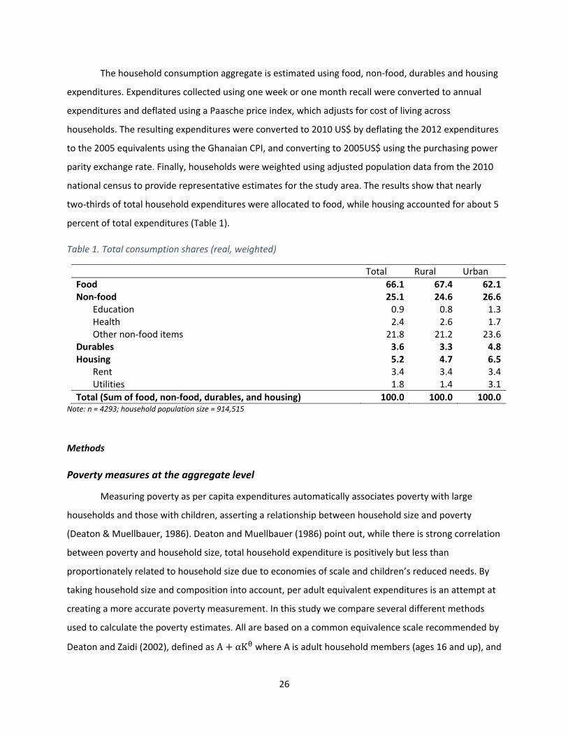
national census to provide representative estimates for the study area. The results show that nearly
two‐thirds of total household expenditures were allocated to food, while housing accounted for about 5
percent of total expenditures (Table 1).
Table 1. Total consumption shares (real, weighted)
Total Rural Urban
Food 66.1 67.4 62.1 Non‐food 25.1 24.6 26.6
Education 0.9 0.8 1.3 Health 2.4 2.6 1.7 Other non‐food items 21.8 21.2 23.6
Durables 3.6 3.3 4.8 Housing 5.2 4.7 6.5
Rent 3.4 3.4 3.4 Utilities 1.8 1.4 3.1
Total (Sum of food, non‐food, durables, and housing) 100.0 100.0 100.0 Note: n = 4293; household population size = 914,515
Methods
Poverty measures at the aggregate level
Measuring poverty as per capita expenditures automatically associates poverty with large
households and those with children, asserting a relationship between household size and poverty
(Deaton & Muellbauer, 1986). Deaton and Muellbauer (1986) point out, while there is strong correlation
between poverty and household size, total household expenditure is positively but less than
proportionately related to household size due to economies of scale and children’s reduced needs. By
taking household size and composition into account, per adult equivalent expenditures is an attempt at
creating a more accurate poverty measurement. In this study we compare several different methods
used to calculate the poverty estimates. All are based on a common equivalence scale recommended by
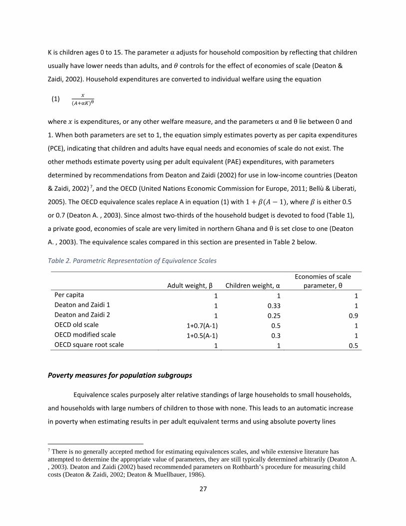
Deaton and Zaidi (2002), defined as A + αK where A is adult household members (ages 16 and up), and
27
K is children ages 0 to 15. The parameter α adjusts for household composition by reflecting that children
usually have lower needs than adults, and controls for the effect of economies of scale (Deaton &
Zaidi, 2002). Household expenditures are converted to individual welfare using the equation
(1) ( )
where is expenditures, or any other welfare measure, and the parameters α and θ lie between 0 and 1. When both parameters are set to 1, the equation simply estimates poverty as per capita expenditures
(PCE), indicating that children and adults have equal needs and economies of scale do not exist. The
other methods estimate poverty using per adult equivalent (PAE) expenditures, with parameters
determined by recommendations from Deaton and Zaidi (2002) for use in low‐income countries (Deaton
& Zaidi, 2002) 7, and the OECD (United Nations Economic Commission for Europe, 2011; Bellù & Liberati,
2005). The OECD equivalence scales replace A in equation (1) with 1 + ( − 1), where is either 0.5
or 0.7 (Deaton A. , 2003). Since almost two‐thirds of the household budget is devoted to food (Table 1),
a private good, economies of scale are very limited in northern Ghana and θ is set close to one (Deaton A. , 2003). The equivalence scales compared in this section are presented in Table 2 below.
Table 2. Parametric Representation of Equivalence Scales
Adult weight, β Children weight, α Economies of scale
parameter, θ
Per capita 1 1 1Deaton and Zaidi 1 1 0.33 1Deaton and Zaidi 2 1 0.25 0.9OECD old scale 1+0.7(A‐1) 0.5 1OECD modified scale 1+0.5(A‐1) 0.3 1OECD square root scale 1 1 0.5
Poverty measures for population subgroups
Equivalence scales purposely alter relative standings of large households to small households,
and households with large numbers of children to those with none. This leads to an automatic increase
in poverty when estimating results in per adult equivalent terms and using absolute poverty lines
7 There is no generally accepted method for estimating equivalences scales, and while extensive literature has attempted to determine the appropriate value of parameters, they are still typically determined arbitrarily (Deaton A. , 2003). Deaton and Zaidi (2002) based recommended parameters on Rothbarth’s procedure for measuring child costs (Deaton & Zaidi, 2002; Deaton & Muellbauer, 1986).

28
(Deaton & Paxson, 1997). Subgroups of the population, such as rural households or those with children,
are even more sensitive to the impact of equivalence scales on poverty estimates. For this reason,
Deaton and Zaidi (2002) recommend normalizing per adult equivalent estimates with a selected base
household type around which to “pivot” so that it results in poverty estimates that are as close as
possible to per capita estimates while still controlling for economies of scale and household
composition. To estimate the “PAE Pivot,” we use the equation
(2) ( ) ∙ ( )( )
where is expenditures and the parameters α and θ are set to 0.33 and 0.9 respectively. The parameters and represent the composition of the base household. For the base household, the
normalized poverty measure is equal to the per capita measure. Since both the mode and median
number of adults and children are 2.0, and are set to these values accordingly (Table 3).
Table 3. Parametric Representation of Equivalence Scales
Children weight, α
Economies of scale parameter, θ
Base adult, Base
children,
PCE 1 1 ‐ ‐
PAE Deaton 0.33 0.9 ‐ ‐
PAE OECD 1 0.5 ‐ ‐
PAE Pivot 0.33 0.9 2 2
Sensitivity Analysis Results
Aggregate level
Per capita and per adult equivalent expenditures are estimated using each of the six methods as
described in Table 2. The results are presented in 2005USD and 2010 USD terms in Table A‐3 and Table
A‐4 respectively, with 2005USD terms used for all subsequent calculations. In estimating the poverty
rate, the distribution of wealth is more important than the mean per capita expenditures. Therefore,
stochastic dominance is used to run a sensitivity analysis on the results. By comparing the poverty
incidence curve (or cumulative distribution function) of each of the methods, we are able to show the
impact of each method on the absolute poverty rates of $1.25 and $2.00 per capita daily expenditures
(Figure 1). The range of expenditures reported is limited to $10 per capita per day for comparison ease
across the different methods.

29
The poverty incidence curve of all five PAE methods are below and to the right of per capita
expenditures across almost the entire range of per capita daily expenditures, with the exception of
several crosses at the high end of the distribution. None of the PAE methods are first‐degree
stochastically dominant to PCE; however, they are all second‐degree stochastically dominant to PCE. The
Kolmogorov‐Smirnov test is also used to compare the distributions of PCE to the alternative methods
and finds that none of the five PAE distributions are equal to the distribution of PCE, indicating that the
PAE distributions are statistically different than the PCE estimate. Correlation coefficients between PCE
and PAE are all above 0.96, suggesting that each method shifts the level of per capita expenditures
uniformly across households (Table A‐1).
From the foregoing, it is evident that reporting per capita expenditures without adult
equivalence scale result in a much higher poverty estimates. For example, at a poverty line of $1.25 per
capita per day, using per capita expenditures will result in a headcount ratio of 22.8% compared to 9.5%,
the next closest poverty rate using Deaton 1 (Figure 2). At a poverty line of $1.25, the OECD square root
scale will result in a much lower poverty rate of 2.1%. Each of the PAE methods also impacts poverty
depth and poverty severity (Table A‐2).
Figure 1. Poverty incidence curve of daily per capita expenditures
0.2
.4.6
.81
Prob
ability
1.250 2 4 6 8 10Per Capita Daily Expenditures
Per Capita Deaton 1
Deaton 2 OECD oldOECD modified OECD square root

30
Figure 2. Comparison of PCE and PAE poverty headcount ratio (%)
Note: n = 4365; household population size = 928,302
Using per adult equivalent expenditures also has an impact on inequality measures. The Lorenz
curve indicates that inequality is similar using all five PAE measures while PCE has a much higher
inequality estimate (Figure 3). The Gini coefficient also shows that equivalence scales have an impact on
inequality, with a Gini coefficient for PCE of 0.516 compared to the PAE estimates between 0.446 and
0.476 (Table A‐2).
It is evident from these results that controlling for household size and composition in northern
Ghana has an impact on each of the poverty measures when estimating overall poverty. We argue that
this is because northern Ghana has a young population, with 44.6 percent of the population under the
age of 15, and a large average household size of almost six people. The young population is a
characteristic indicative of rapid population growth. A high population growth rate is common in
developing countries where the death rate begins to fall more rapidly than the birth rate, due to
economic development and multiple related factors such as increased food production, improvements
in trade, and advances in medicine and hygiene. This period of rapid population growth is referred to as
the demographic transition, and lasts for multiple decades before the population stabilizes as birth and
death rates converge (Nafziger, 2006). All indications suggest that northern Ghana is in this period of
demographic transition, leading to a young population, large households, and therefore large disparity
between poverty rates when using equivalence scales.
22.8
9.56.1
9.0
3.92.1
42.8
25.5
17.9
24.8
14.2
9.0
0
5
10
15
20
25
30
35
40
45
Per capitaexpenditures
Deaton 1 Deaton 2 OECD, oldscale
OECD,modified scale
OECD, squareroot scale
Per
cen
t B
elow
th
e P
over
ty L
ine
$1.25 poverty line $2.00 poverty line

31
Figure 3. Lorenz curve of daily per capita expenditures
Although household size and composition are not entirely separable, we attempt to
differentiate the impacts of both parameters on poverty estimates. To do this we compare PCE to the
OECD square root method which essentially only corrects for household size and the Deaton 1 method
which only corrects for household composition.
First, we compare the changes in the poverty rate resulting from changes in household size
(Figure 4). The poverty rates are identical in households with one person regardless of the method.
However, as the number of household members increases, the poverty rate increases exponentially for
per capita expenditures, while it increases more reasonably for the other two methods. Figure 5
conducts the same experiment but using number of children instead of household size. Once again,
there is a great divergence between the PCE and the both PAE methods.
0.2
.4.6
.81
L(p
)
0 .2 .4 .6 .8 1Percentiles (p)
45° line Per Capita
Deaton 1 Deaton 2
OECD old OECD modified
OECD square root

32
Figure 4. Poverty rates of $1.25 per day by household size
Note: n = 4365; household population size = 928,302
These results reveal how the PCE method is heavily affected by household size and composition.
Alternatively, the PAE methods control for economies of scales and household size in an attempt to
discover rather than assert the relationship between poverty and household size and composition
(Deaton & Muellbauer, 1986). The relationship between household size and composition and poverty
becomes even more important to understand when we estimate child or elderly poverty, or compare
rural to urban poverty.
To investigate the matter further, we compare the mean household size and number of children
per household to several different household types (Table 4). Households with children are significantly
larger than those without, just as households without elderly and rural household are significantly larger
than households with elderly and urban households respectively.
0%
5%
10%
15%
20%
25%
30%
35%
40%
45%
1 2 3 4 5 6 7+
Hea
dco
un
t p
over
ty r
ate
Household size
Per capita expenditures
Per adult equivalent expenditures Deaton 2
Per adult equivalent expenditures OECD square root

33
Figure 5. Poverty rates of $1.25 per day by children per household
Note: n = 4365; household population size = 928,302
Table 4. Mean household size and children per household
With Children
Without Children
With Elderly
Without Elderly Rural Urban Total
Household size 6.4*** 2.1 5.5 6.3*** 5.9*** 4.8 5.6
Children per household ‐ ‐ 2.6 2.7 2.9*** 2.0 2.7 Note: n = 4365; household population size = 928,302; *, **, and *** indicates significantly different at the 0.10, 0.05 and 0.01 levels respectively using an Adjusted Wald test.
PAE Pivot household results
As noted previously, the use of equivalence scales has a large impact on overall poverty
measures. This leads us to estimate expenditures as PAE Pivot, normalizing per adult equivalent
estimates with a selected base household. While previous PAE estimates resulted in much lower poverty
estimates than PCE, the PAE Pivot mean poverty headcount ratio is $3.48 per daily capita, compared to
$4.01 per daily capita for PCE and $5.22 per daily capita for the nearest PAE estimate (Table A‐3). We
run a sensitivity analysis to compare the PCE to the PAE Deaton and PAE OECD square root scale, using
stochastic dominance (Figure 6). The per capita daily expenditures on the x‐axis are limited to $10 per
capita per day for ease of comparison.
0%
10%
20%
30%
40%
50%
60%
0 1 2 3 4 5 6 7+
Hea
dco
un
t p
over
ty r
ate
Children per household
Per capita expenditures
Per adult equivalent expenditures Deaton 2
Per adult equivalent expenditures OECD square root

34
Figure 6. Poverty incidence curve of daily per capita expenditures
No method is first‐degree stochastically dominant to the per capita expenditures method.
However, both the PAE Deaton and PAE OECD methods are below the PCE method, and therefore are
second‐degree stochastically dominant. The Kolmogorov‐Smirnov test is also used to compare the
distributions of PCE to the alternative methods, and finds that none of the distributions of the PAE
methods are equal to the PCE. Therefore, while it appears that the PAE Pivot method provides results
that are more similar to the PCE method, the distributions are still statistically different. However, the
PAE Pivot measures are much closer than other PAE methods to PCE (Deaton & Zaidi, 2002). The PAE
Pivot method also results in a poverty gap and squared poverty gap that are only slightly higher than the
PCE method (Table A‐2), but it does not impact inequality (Figure A‐1).
Results for population subgroups
Child and elderly poverty
As noted earlier in Table 4, households with children are significantly larger than those without,
while households with elderly are significantly smaller than households without. For this reason, PAE
methods result in poverty headcount ratios that are much lower than PCE measures. However, using a
pivot household results in headcount ratios that are much closer to PCE (Table 5). A graphical
0.2
.4.6
.81
Prob
abili
ty
1.250 2 4 6 8 10Per Capita Daily Expenditures
PCE PAE DeatonPAE OECD PAE Pivot
35
representation of the impact of PAE Pivot on households of different size and the number of children
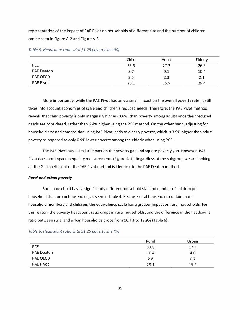
can be seen in Figure A‐2 and Figure A‐3.
Table 5. Headcount ratio with $1.25 poverty line (%)
Child Adult Elderly
PCE 33.6 27.2 26.3 PAE Deaton 8.7 9.1 10.4 PAE OECD 2.5 2.3 2.1 PAE Pivot 26.1 25.5 29.4
More importantly, while the PAE Pivot has only a small impact on the overall poverty rate, it still
takes into account economies of scale and children’s reduced needs. Therefore, the PAE Pivot method
reveals that child poverty is only marginally higher (0.6%) than poverty among adults once their reduced
needs are considered, rather than 6.4% higher using the PCE method. On the other hand, adjusting for
household size and composition using PAE Pivot leads to elderly poverty, which is 3.9% higher than adult
poverty as opposed to only 0.9% lower poverty among the elderly when using PCE.
The PAE Pivot has a similar impact on the poverty gap and square poverty gap. However, PAE
Pivot does not impact inequality measurements (Figure A‐1). Regardless of the subgroup we are looking
at, the Gini coefficient of the PAE Pivot method is identical to the PAE Deaton method.
Rural and urban poverty
Rural household have a significantly different household size and number of children per
household than urban households, as seen in Table 4. Because rural households contain more
household members and children, the equivalence scale has a greater impact on rural households. For
this reason, the poverty headcount ratio drops in rural households, and the difference in the headcount
ratio between rural and urban households drops from 16.4% to 13.9% (Table 6).
Table 6. Headcount ratio with $1.25 poverty line (%)
Rural Urban
PCE 33.8 17.4 PAE Deaton 10.4 4.0 PAE OECD 2.8 0.7 PAE Pivot 29.1 15.2

36
Conclusion
The study’s results show that the use of adult equivalence scales, which control for household
economies of scale and composition, has a large impact on poverty estimates. Because household size
and composition differ across different household types such as rural and urban, or those with or
without children, the use of equivalence scales becomes even more compelling when comparing
subgroups of the population. We find that calculating poverty measures by normalizing per adult
equivalent expenditures by a standard pivot household creates poverty measures similar to PCE
estimates. In the case of Ghana, estimating the headcount poverty ratio in per adult equivalent terms
reveals a lower child poverty rate and higher elderly poverty rate in comparison to adult poverty.
Based on these results, we suggest that poverty measures estimated using PCE must be
subjected to a sensitivity analysis using PAE measures, especially in developing countries with
demographics similar to northern Ghana. Future research should explore at what point in the
demographic transition the use of equivalence scales is most compelling, and which standard
parameters of equivalence scales should be used to control for household size and composition.
References
Bellù, L. G., & Liberati, P. (2005). Equivalence Scales: Subjective Methods. Rome: EASYPol, FAO.
Buhmann, B., Rainwater, L., Schmaus, G., & Smeeding, T. M. (1988). Equivalence Scales, Well‐Being,
Inequality, and Poverty: Sensitivity Estimates Across Ten Countries using the Luxenbourg Income
Study (LIS) Database. Review of Income and Wealth, 34(2), 115‐142.
Burkhauser, R. V., Smeeding, T. M., & Merz, J. (1996). Relative Inequality and Poverty in Germany and
the United States Using Alternative Equivalence Scales. Review of Income and Wealth, 42(4),
381‐400.
Coulter, F. A., Cowell, F. A., & Jenkins, S. P. (1992). Equivalence Scale Relativities and the Extent of
Inequality and Poverty. The Economic Journal, 1067‐1082.
Datt, G., & Ravallion, M. (1998). Why Have Some Indian States Done Better than Others at Reducing
Rural Poverty? Economica, 65, 17‐38.
Deaton, A. (2003). Household Surveys, Consumption, and the Measurement of Poverty. Economic
Systems Research, 135‐159.

37
Deaton, A. S., & Muellbauer, J. (1986). On Measuring Child Costs: With Applications to Poor Countries.
Journal of Political Economy, 94(4), 720‐743.
Deaton, A., & Paxson, C. (1997). Poverty among children and the elderly in developing countries.
Research Program in Development Studies, Princeton University.
Deaton, A., & Zaidi, S. (2002). Guidlines for Constructing Consumption Aggregates for Welfare Analysis.
Washington, DC: World Bank.
Éltetõ, Ö., & Havasi, É. (2002). Impact of Choice of Equivalence Scale on Income Inequality and on
Poverty Measures. Review of Sociology, 8(2), 137‐148.
Ferreira, M. L., Buse, R. C., & Chavas, J.‐P. (1998). Is There Bias in Computing Household Equivalence
Scales? Review of Income and Wealth, 44(2), 183‐198.
Haughton, J., & Khandker, S. R. (2009). Handbook on Poverty and Inequality. Washington, DC: The World
Bank.
Hunter, B. H., Kennedy, S., & Biddle, N. (2004). Indigenous and Other Australian Poverty: Revisiting the
Importance of Equivalence Scales. The Economic Record, 80(251), 411‐422.
Lancaster, G., Ray, R., & Valenzuela, M. R. (1999). A Cross‐Country Study of Equivalence Scales and
Expenditure Inequality on Unit Record Household Budget Data. Review of Income and Wealth,
45(4), 455‐482.
Lanjouw, P., & Ravallion, M. (1995). Poverty and Household Size. The Economic Journal, 105, 1415‐1434.
Meenakshi, J., & Ray, R. (2002). Impact of household size and family composition on poverty in rural
India. Journal of Policy Modeling, 24, 539‐559.
Nafziger, W. E. (2006). Economic Development. New York: Cambridge University Press.
Pollak, R. A., & Wales, T. J. (1979). Welfare Comparisons and Equivalence Scales. The American Economic
Review, 69(2), 216‐221.
Reddy, S., Visaria, S., & Asali, M. (2006). Inter‐country Comparisons of Poverty Based on a Capability
Approach: An Empirical Exercise. Brasilia: Working Paper No. 27, International Poverty Centre,
UNDP.
Short, K., Garner, T., Johnson, D., & Doyle, P. (1999). Experimental Poverty Measures: 1990 to 1997.
Washington, DC: U.S. Government Printing Office.
Streak, J. C., Yu, D., & Van der Berg, S. (2009). Measuring Child Poverty in South Africa: Sensitivity to the
Choice of Equivalence Scale and an Updated Profile. Social Indicators Research(94), 183‐201.
United Nations Economic Commission for Europe. (2011). Canberra Group Handbook on Household
Income Statistics, Second Edition. Geneva: United Nations.

38
Visaria, P. (1980). Poverty and Living Standards in Asia: An Overview of the Main Results and Lessons of
Selected Household Surveys. Washington, DC: World Bank.
White, H., & Masset, E. (2002). Constructing the Poverty Profile: An Illustration of the Importance of
Allowing for Household Size and Composition in the Case of Vietnam.

39
Appendix
Figure A‐1 Lorenz curve of daily per capita expenditures
0.2
.4.6
.81
L(p
)
0 .2 .4 .6 .8 1Percentiles (p)
45° line PCE
PAE Deaton PAE OECD
PAE Pivot

40
Figure A‐2. Poverty rates of $1.25 per day by household size
Note: n = 4365; household population size = 928,302
Figure A‐3. Poverty rates of $1.25 per day by children per household
Note: n = 4365; household population size = 928,302
0%
5%
10%
15%
20%
25%
30%
35%
40%
45%
1 2 3 4 5 6 7+
Hea
dco
un
t p
over
ty r
ate
Household size
PCE PAE Deaton PAE OECD PAE Pivot
0%
10%
20%
30%
40%
50%
60%
0 1 2 3 4 5 6 7+
Head
count poverty rate
Children per household
PCE PAE Deaton PAE OECD PAE Pivot

41
Table A‐1. Correlation coefficients of per capita and per adult equivalent expenditures
Per capita expenditures Deaton 1 Deaton 2
OECD, old scale
OECD, modified scale
OECD, square root scale
Per capita expenditures 1
Deaton 1 0.978 1
Deaton 2 0.988 0.998 1
OECD, old scale 0.993 0.993 0.995 1
OECD, modified scale 0.979 0.994 0.991 0.996 1
OECD, square root scale 0.961 0.985 0.977 0.985 0.995 1
Table A‐2. Comparison of PCE and PAE on the headcount ratio, poverty gap, squared poverty gap, and Gini coefficient (poverty line = $1.25 per day)
Headcount ratio Poverty gap Squared poverty gap Gini
coefficient
Per capita 22.8 7.1 3.2 0.516 Deaton 1 9.5 2.7 1.1 0.475 Deaton 2 6.1 1.5 0.6 0.460 OECD old scale 9.0 2.4 1.0 0.476 OECD modified scale 3.9 1.0 0.4 0.456 OECD square root scale 2.1 0.5 0.2 0.446 PAE Pivot 21.3 6.5 2.9 0.464

42
Table A‐3. Per capita and per adult equivalent expenditures (2005USD/capita/day)
Mean Median1Std.
Deviation1 Minimum Maximum
Per capita 3.59 b, c, d, e, f 2.21 5.30 0.10 201.43
Deaton 1 4.67 a, c, d, e, f 3.28 5.74 0.16 201.43
Deaton 2 5.38 a, b, d, e, f 3.92 6.20 0.20 201.43
OECD old scale 4.79 a, b, c, e, f 3.38 6.82 0.22 201.43
OECD modified scale 5.94 a, b, c, d, f 4.39 5.99 0.17 201.43
OECD square root scale 6.77 a, b, c, d, e 5.12 7.59 0.26 201.43 Note: n = 4365; household population size = 928,302; a, b, c, d, e, and f indicates significantly different mean expenditures
compared Per capita, Deaton 1, Deaton 2, OECD old scale, OECD modified scale, OECD square root scale respectively at the 0.05
level using Adjusted Wald test; 1: Based only on 4293 observations.
Table A‐4. Per capita and per adult equivalent expenditures (2010USD/capita/day)
Mean Median1Std.
Deviation1 Minimum Maximum
Per capita 4.01 b, c, d, e, f 2.58 5.91 0.11 224.90
Deaton 1 5.22 a, c, d, e, f 3.67 6.41 0.18 224.90
Deaton 2 6.01 a, b, d, e, f 4.38 6.92 0.22 224.90
OECD old scale 5.35 a, b, c, e, f 3.77 7.61 0.25 224.90
OECD modified scale 6.63 a, b, c, d, f 4.91 6.68 0.18 224.90
OECD square root scale 7.56 a, b, c, d, e 5.72 8.48 0.29 224.90 Note: n = 4365; household population size = 928,302; a, b, c, d, e, and f indicates significantly different mean expenditures
compared Per capita, Deaton 1, Deaton 2, OECD old scale, OECD modified scale, OECD square root scale respectively at the 0.05
level using Adjusted Wald test; 1: Based only on 4293 observations.

43
A Cautionary Note on Comparing Poverty Prevalence Rates
Vincent Amanor‐Boadu, Kara Ross and Yacob Zereyesus
Department of Agricultural Economics
Kansas State University
March 2015
Introduction
Household expenditures, used as a proxy for income, were the data used to estimate the
prevalence of poverty in the four northernmost regions of Ghana that formed the Zone of Influence for
the population‐based survey (PBS) conducted for USAID in Ghana in 2012.8 Household expenditure was
categorized into four groups: food; housing; durables; and non‐durables. Non‐durables include such
goods as fuel, transportation, education and health care, whether purchased, home produced or
received as gifts. Durables include household items that last more than a few years – refrigerators,
radios, automobiles, bicycles, etc. Housing covered rent and implicit cost of owned dwelling while food
expenditures included all food consumed by the household whether purchased, produced or received as
gifts.
PBS respondents’ recalled their household expenditures on items in the different categories for
different periods in the Ghana Cedi. These were annualized and aggregated to produce total household
expenditure. Dividing the total household expenditure by the household size and again by 365
produced the average daily per capita household expenditure. To ensure international comparability,
the estimated average daily per capita household expenditure was converted from the 2012 Ghana Cedi
into 2005 US dollars using Bank of Ghana consumer price index (CPI) and World Bank published
purchasing power parity (PPP) exchange rate or conversion factor.9 The PPP conversion factor was
0.447. With the 2000 CPI set to 100, the Bank of Ghana‐reported CPI in 2005 and 2012 were
respectively 183.7 and 412.4. These parameters provided the inputs for completing the conversion of
2012 consumption expenditures in Ghana Cedi into 2005 US dollars.
8 Using expenditures as a proxy for income is valid as long as it is assumed that the household has no
savings. That is, net income, defined as income after all involuntary expenses, such as taxes and imposed fines, is total expended on food, housing, durables and non-durables without any left over as savings from one period to another.
9 For full and detailed description of the approach used, see Zereyesus, Y., K. Ross, V. Amanor-Boadu and T. Dalton. Baseline Feed the Future Indicators for Ghana, 2012, Manhattan, KS: Kansas State University Press, 2014.

44
The average daily per capita household total expenditure was $4.01 and its distribution across
the four categories is presented in Figure 1. The figure shows that the average daily per capita
household expenditure on food and non‐durables was about 88 percent of the average household daily
per capita expenditure while housing and durables accounted for the remaining 12 percent. That food
accounted for 61.3 percent of the average daily per capita household expenditure is in line with what
has been found by other studies.10 Analyzing the data at the household level reflects the reality of
shared and collective consumption in the majority of the items in the expenditure categories. This
reveals the embedded scale economies associated with household consumption, a point that should not
be ignored in assessing the prevalence of poverty.
Figure 11: Distribution of Average Daily per Capita Household Expenditure across the Four Expenditure Categories
Research Problem
The motivation for this discussion paper was explaining why differences exists across poverty
prevalence rates measured for particular countries. For example, while the 2012 PBS produced a
poverty prevalence rate of 22.2 percent, the Ghana Living Standards Survey of 2005/2006 posted rates
between 29.5 percent and 87.9 percent for the regions in the PBS.11 The paper has two major
10 See Mussa, R. (2014). “Household Expenditure Components and the Poverty and Inequality Relationship
in Malawi,” African Development Review-Revue Africaine De Developpement, 26(1): 138-147. 11 International Monetary Fund and National Development Planning Commission (2009). Ghana: Poverty
Reduction Strategy Paper - 2006 Annual Progress Report, Washington, DC: IMF Country Report No. 09/237.
FoodGHS 2.46
Non‐durablesGHS 1.07
Housing0.20
DurablesGHS 0.24
0% 10% 20% 30% 40% 50% 60% 70% 80% 90% 100%
Share of Expenditure

45
objectives. First, it seeks to present in an independent document how the poverty prevalence rate of
22.2 percent for the 2012 PBS in the area above Latitude 8⁰N in Ghana was estimated.12 The second
objective is to provide a systematic explanation of why this estimate may differ from other estimates,
such as the one presented in the Ghana Living Standards Survey of 2005/2006. In the end, the paper
seeks to enhance awareness among researchers in this field about the potential sources for differences
and sharpen policymakers’ appreciation about how these rates get estimated and why differences may
exist. It is hoped that the paper would help both researchers and policymakers develop a more careful
approach when comparing poverty rate estimates from different studies and across time.
Measuring Poverty: Individuals versus Households
Prevalence of poverty has been measured traditionally as the number of individuals in a
population with income or expenditures below an established poverty line or threshold. Most
developing countries use the poverty line established by the World Bank – US$1.25 per capita per day in
2005 purchasing power parity (PPP). This individual per capita expenditure approach has become the
dominant approach in many poverty estimates, including the ones reported by the World Bank.
Proponents of the individual per capita consumption approach argue that it addresses
differences in household sizes.13 However, its critics contend that it ignores the scale economies
associated with household consumption.14 Individuals in a household do not purchase and consume
their meals independent of other members of their household. By purchasing as a group (the
household), they gain benefits that are unavailable to them as individuals, e.g., bulk purchasing,
collective preparation, etc. This is how the household gains scale economies in consumption. Others
have also argued that measuring poverty by individual per capita expenditures ignores the composition
of the household, i.e., the number of adults and children as well as the specific age distribution of the
household.15 The US, for example, recognizes the household type – size and age distribution – in the
estimation of prevalence of poverty. Deaton and Zaidi and Regier et al., among others, have, thus,
argued that consumption expenditures must be measured on adult‐equivalent basis to address the
12 See Zereyesus et al. (2014). 13 Haughton, J. and S.R. Khandker (2009). Handbook on Poverty and Inequality. Washington, DC: The
World Bank. 14 Deaton, A. (2003). “Household Surveys, Consumption, and the Measurement of Poverty,” Economic
Systems Research, 15(2): 135-159. 15 Meenakshi, J. and R. Ray. (2002). “Impact of Household Size and Family Composition on Poverty in Rural
India,” Journal of Policy Modeling, 24: 539-559.

46
presence of children in the household in order to attain a more accurate measure of the prevalence of
poverty in a population.16
The fact that there are differences in consumption among adults of different age cohorts must
not be overlooked. For example, adults over 70 years may have different consumption patterns than
those who are below 50 years. These adults may spend less on food and clothing but more health
products, for example. Similarly, children who are between 14 years and 18 years may have very
different consumption patterns from those who are below six years. These teenagers may consume
more education, fashionable clothing and more food than toddlers whose expenditures may be non‐
pecuniary and yet time intensive.
The foregoing observations of potential sources of differences in households point to the
overestimation risk associated with using the individual per capita expenditure to measure poverty
rates, especially in societies where children form a large proportion of the population. Regier et al.
(2014) show that using the adult equivalent expenditures not only compensates for the large proportion
of children in the study area but also reduces the disparity across the population.
The weakness of the individual per capita approach may be summarized into two cogent foci: (i)
It does not account for children in the population; and (ii) It does not recognize the scale economies that
are associated with the nature of consumption in societies. There is an ongoing debate on how to treat
the children question.17 What is the appropriate weight that may be used for children of different ages?
It will not be accurate to assign the same weight to babies and infants as teenagers. This debate implies
that any attempt to deal with the adult equivalency could prove contentious. How accurate is it to
assign the same weight to all adult age cohorts, especially given that older adults tend to consume less
of certain goods and services and more of others?18
The scale economies’ effect is one that should be easy to deal with. And that is the approach
adopted in the 2012 PBS study. While we recognized the differences in consumption across age cohorts,
we also knew that the nature of the data meant isolating and accounting for such differences was not
16 Deaton, A. and S Zaidi (2002). Guidelines for Constructing Consumption Aggregates for Welfare Analysis,
Washington, DC: World Bank; Regier, G., Y. Zereyesus, T. Dalton and V. Amanor-Boadu (2014). “Do Adult Equivalence Scales Matter in Poverty Estimates? A Ghana Case Study,” Department of Agricultural Economics, Kansas State University, Working Paper, 2014.
17 See Regier at al. (2014) referenced above. 18 See Lee, S., S-H Sohn, F. Rhee, Y.G. Lee, and H. Zan, (2014). “Consumption Patterns and Economic
Status of Older Households in the United States,” Monthly Labor Review (Sep): 1B-22B.

47
going to be easy because of the sample size. Conducting an analysis that was cognizant of scale
economies from consumption demanded that the analysis be done at the household level. It is not as
perfect as applying the appropriate weights to each individual in the household, but it is much better
than not recognizing the scale economies in household consumption. In using this approach, it is
assumed that when the average daily per capita household expenditure was below the poverty line,
then the household, not its individual members, is counted. This implies that economies of scale in
consumption are recognized and incorporated in the estimation of poverty prevalence.
Let us illustrate this with a simple example. Consider a sample with five households, A, B, C, D
and E with four, six, 10, 12 and 14 members respectively. Suppose that the total consumption
expenditure for the five households at a particular time is the same, $10. This implies that average per
capita expenditure for households range from $2.50 for Household A to $0.71 for Household E (Figure
2). With a total number of people in the example of 46 people, the foregoing would suggest a poverty
prevalence rate of about 78.3 percent (i.e., 36 of the 42 people) when consumption economies of scale
are ignored. By recognizing consumption scale economies and conducting the analysis at the household
instead of the individual level, the prevalence rate is now 60 percent – that is, three households out of
the five have average daily per capita household expenditures of under $1.25. This is 18.2 percent lower
than when the consumption scale economies are ignored, increasing the estimated poverty by 30.4
percent. While the larger number might look good for those involved in the poverty business (because
it offers a larger market of poor people), it presents significant risks in developing and implementing
policies that often target households and not individuals. This lack of consistency may explain the
difficulty of securing sustainable poverty reduction initiatives and programs in many places.

48
Figure 12: Illustration of Individual and Household Approaches to Prevalence of Poverty Measures
In the foregoing light, we estimated the average daily per capita household expenditure for the
qualifying 4,365 households in the population‐based survey sample.19 Any household with an average
daily per capita household expenditure of less than $1.25 in 2005 PPP was coded as being below the
poverty line as established by the World Bank. Based on this approach, which recognizes the scale
economies in household consumption, we estimated the poverty prevalence rate as 22.2 percent, i.e.,
963 of the 4,365 households. The prevalence of poverty for the same dataset using the individual per
capita approach was 30.2 percent. This is equivalent to a poverty prevalence rate that is approximately
36.0 percent higher, which in line with our earlier argument that ignoring scale economies of
consumption inflates the poverty rate.
Comparability across Time and Studies
A major input in the development of prevalence of poverty rates is the purchasing power
parity.20 The PPP exchange rate allows the cost of a basket of goods consumed in one country to be
appropriately compared with a similar basket of goods in another country. Calculation of PPP exchange
rates is a complex process and it is carefully done for the international community by the World Bank.
19 The difference in the sample size is a result of unavailable information or incomplete data on certain
households. 20 For an overview of the role purchasing power parity plays in estimating prevalence of poverty rates, see
Zereyesus, Y. and V. Amanor-Boadu (2015). Macroeconomic Effects on Poverty Rate: A Case Study of Northern Ghana, Working Paper, Department of Agricultural Economics, Kansas State University.
0
2
4
6
8
10
12
14
16
$‐
$0.50
$1.00
$1.50
$2.00
$2.50
$3.00
4 6 10 12 14
Number of Peo
ple
Average Per Capita Expen
diture
Household Size
Average Expenditure Poverty Line Number of People

49
As a result of changes in the macroeconomic environment in the numerous countries included in the
estimation, PPP exchange rates are changed periodically. Changes in the PPP exchange rates can
significantly affect poverty prevalence even if nothing else has changed in the lives of the affected
people. This potential effect of the PPP on poverty prevalence rates underscores the non‐comparability
of poverty prevalence rates within any particular country across time without the proper adjustments to
the reference PPP.21 Yet, the temptation to compare these rates is often difficult to resist and the
difficulty of making the right adjustments means that they are often overlooked. However, for the most
part, the people making the comparisons are just unaware of the fact that they are comparing apples
and oranges.
Another risk that often escapes many analysts is comparing poverty prevalence rates across
studies. There are two dimensions of potential errors in these comparisons. First is the time difference
factor. For example, the population‐based survey for the region above Latitude 8⁰N was conducted in
2012 while the latest Ghana Living Standards Survey (GLSS) at the time was conducted 2006. It is very
tempting for analysts and policymakers who are trying in good faith to develop trends for the results of
poverty intervention efforts to take the two rates and compare them without paying careful attention to
the time difference. The time effect, already discussed, presents different PPP exchange rates and
different CPI. Without standardizing these parameters, any comparisons are like comparing apples to
oranges.
The other major sources of potential comparison errors are the statistical foundations of
conducting such studies. Recall that the estimation of consumption expenditures begins with the
drawing of a sample of households from whom consumption data are collected. The sampling process is
often influenced by specific research objectives. In the case of the PBS, a two‐stage stratified sampling
approach was used. It involved stratifying the study area by the presence or absence of an intervention
project that was of interest to USAID at the time of the study – the Resilience in Northern Ghana (RING)
Project. The second stage involved randomly selecting a specific number of enumeration areas from
each stratum and then randomly selecting a number of households from each enumeration area. The
number of enumeration areas and households selected was guided by particular statistical power
assumptions. The expectation is that by carefully following the defined sampling process, it will be
possible to draw a random sample that would produce a normal distribution as its underlying
21 The World Bank warns that inter-temporal comparisons of poverty prevalence rates within countries not be
done. See statement at http://data.worldbank.org/indicator/SI.POV.DDAY.

50
distribution. Because normal distribution is assumed in most of these research, it is never tested in
further analyses and in extrapolations from the sample results.22
Whenever two samples are drawn from a population and the assumption of normal distribution
is violated, the means for those samples can be expected to be different. Because researchers assume
normal distribution of their samples and hardly ever test the veracity of this assumption, differences in
estimates from different samples may in fact be due solely to sampling bias and not estimation errors.
Let us illustrate this with a hypothetical example. Suppose there are equal number of black and white
balls in a jar with 100 balls, and we pull two samples at different times of 20 balls from the jar. Assume
that the time periods are close enough so that the risk of any balls being lost is minimized or eliminated
but long enough so that the drawn balls can be placed back in the jar before the second sample is
drawn. It is both plausible and possible that the number of black and white balls drawn in the two
samples would be different despite their equal probability of being selected.23 If we repeat this
experiment numerous times, the average of the mean proportion of the colors will approach their true
probability.
It is expensive, if not impractical, to draw more than one sample for human studies such as
estimating the prevalence of poverty. This is because humans are by nature inherently different from
each other even when they have very similar characteristics. In survey research, research subjects may
refuse to participate, fail to understand the same question in the same way because of some personal
difficulties, choose not to answer particular questions, etc. When these challenges occur, the
assumption of normality may be violated and no two samples from the population will reflect the same
mean and/or standard deviation. Problems such as skewing and/or kurtosis of the sample are non‐
trivial but they are hardly reported in prevalence of poverty estimates because of the inherent
assumption of normality. Researchers do this neither out of mischievousness, some nefarious reason
nor ignorance but merely because of lack of awareness of how powerful the effect of the normality
assumption is on cross‐study comparisons of estimates.
22 Morris, C. H., Jr. (2014). The Value, Degree, and Consistency of Kansas Crop Farms’ Relative
Characteristics, Practices, and Management Performances, Manhattan, KS: Department of Agricultural Economics, Kansas State University, Unpublished M.S. Thesis. Available at http://krex.k-state.edu/dspace/handle/2097/17631.
23 We assume that the person making the selection is blindfolded and has no way of biasing the selection process.

51
If the comparisons should not be done, how do we verify if policy interventions are achieving
their desired objectives? It is critical to estimate poverty prevalence using the same poverty line and
PPP exchange rate over time. This allows for an analysis of changes in the rate because the rates are
based on the same reference PPP exchange rate. For inter‐study comparisons, we have noted that spot
estimates are expected to be different because of sampling differences and violations of statistical
assumptions. However, tracking the poverty prevalence rate changes across studies that have been
conducted under similar conditions over time could allow some comparisons to be made. The GLSS
(2005/2006) and more recent GLSS (2012/2013) had a poverty prevalence rate of 16.0 percent and 8.4
percent respectively. This is equivalent to about 50 percent reduction in poverty rate over seven years.
Suppose another study with the same start and end points shows a reduction around 50 percent
reduction, then it is plausible to accept their comparability even though their absolute measures of
poverty prevalence rates are different. However, if the start and end points are different, then the only
way to gain some idea about comparability is to rebase the poverty prevalence rates in both studies to
common start and end time periods so that the PPP exchange rates could be harmonized. This is not
easy to do, even when one has the raw data available because of how researchers often choose to deal
with such challenges as outliers in their attempts to generate some semblance of normal distribution on
their datasets.
Conclusions
The baseline poverty prevalence rate for the focus area for USAID interventions in Ghana was
22.2 percent. It was measured at the household level and in so doing recognized the consumption scale
economies’ effect that households enjoy over individuals. These economies of scale in consumption
suggest that if poverty rates are to be accurately measured at the individual level, it will be necessary to
make adjustments to the expenditures to recognize the loss of the scale economies. We argued that
while recognizing differences in consumption across age cohorts would improve the metric, the
empirical challenges make this household level analysis far superior to the individual level analysis that
is prevalent in the literature and in policy circles.
We also showed that changes in the PPP exchange rate to recognize relative changes in the
macroeconomic conditions in particular countries may affect poverty rate measures without actual
change in people’s wellbeing. Therefore, we agreed with the World Bank to avoid inter‐temporal
comparison of poverty prevalence rates unless they can be re‐estimated to have the same base PPP
exchange rate.

52
We also argued that the appropriate care be taken in comparing poverty prevalence rates across
studies because of differences in samples and their distribution biases. It is realistic to expect
differences in the core statistics of samples, i.e., their means and standard deviations, when the samples
are different and their normal distribution assumption is violated. We noted that normality is assumed
hold in samples and are, therefore, hardly tested in the estimates. As a result, researchers are often
unaware when they are violated. Without recognizing this, it is not only plausible but possible to have
two samples drawn from the same population having significantly different statistics. The lesson from
this is that comparing point statistics may be fruitless and contribute little valuable information unless
these potential sources of discrepancy are controlled. However, comparing changes in two point
estimates that have been estimated using the same approaches could provide valuable insights.
For the Economic Growth Office and its Development Partners in Ghana, we believe the most
important focus should be on whether they are able to achieve their target poverty reductions. The
Economic Growth Office, for example, has a 20 percent target reduction in poverty over five years from
the baseline estimated in 2012. This implies that by 2017, the household poverty prevalence rate in the
study area should be no higher than 17.76 percent if the poverty line of $1.25 is maintained and the
necessary PPP exchange rate adjustments are made. Given the non‐comparability arguments presented
here, it would seem that focusing on the interventions that produce the target reductions to which we
have committed is the most effective strategic course.

53
Securing Africa’s Middle Class: The Case of Northern Ghana
Vincent Amanor‐Boadu, PhD
Department of Agricultural Economics
Kansas State University, Manhattan, KS 66506
April 2015
Abstract
One indicator of how well economic development‐inducing poverty reduction is occurring is middle class
growth. Recent studies show that the middle class has been increasing in virtually all countries in Sub‐
Saharan Africa. Yet, there is no clear empirical appreciation of the factors driving this growth and how
sustainable it is. This study seeks to address this knowledge gap by identifying the socio‐economic
factors supporting the growth in the middle class in Sub‐Saharan Africa using northern Ghana as a case
study. The results show that rural and urban locales, household size, education and food share of total
expenditures influence the probability of being in the middle class. For example, the odds of being in
the middle class when one has some education is about 2.4 times higher than not having any education.
Similarly, the odds of an urban resident being in the middle class is about three times higher than that of
a rural resident. A percentage increase in the household size reduces the probability of being in the
middle class by almost 5 percent. Finally, a percentage point increase in food share of total
expenditures increases the probability of being in the middle class by more than 16 percent. The results
help identify specific strategic actions that may be pursued by individuals, governments and
development agencies if securing the middle‐income class is recognized as a critical factor in achieving
poverty reduction and income enhancing objective while contributing to building sustainable economic
development in developing countries.
Keywords: Middle‐income class; middle class; poverty; economic development; infrastructure
Introduction
Despite a near unanimous agreement about the mutual benefits from the economic
development support advanced economies provide developing, the debate about implementation
strategies continues. Some argue that foreign aid displaces public savings and creates dependency
(Quattara, 2007). Harvey and Lind (2005) argued the opposite of the dependency risk, noting that aid
delivery is often not transparent or reliable enough to engender dependency. However, Farag et al.
(2005) note that foreign aid, especially in low‐income countries, does indeed displace government
spending instead of enhancing it. Others have criticized the role of technology transfers, arguing they
create unsustainable prosperity because they often include significant import components that keep the
recipient countries dependent on the donor countries (Stewart, 1990). In a piece done for CNN, Ntale

54
(2013) notes that “Large amounts of aid money never actually leave rich countries.” They are used to
cover debt cancellation, pay for expatriates working in technical support roles, cover tuition and
accommodation, and purchase products and equipment manufactured in donor countries. For example,
almost 70 percent of Italy's $2 billion bilateral aid in 2011 stayed in Italy – as expenditures on refugee
costs and debt relief (Ntale, 2014). Development Initiatives (2013) also shows that less than $2.5 billion
of the $7.5 billion in aid received by the Democratic Republic of Congo in 2011 actually made it into the
country.
The foregoing criticisms notwithstanding, focused attention on poverty reduction over the past
few decades has produced some very tangible – and hopefully – sustainable results. For example, the
infant mortality rate, measured as the number of children dying before reaching their first birthday per
1,000 births, in Sub‐Saharan Africa declined from 136.3 in 1973 to 61 in 2013. Between 1990 and 2013,
maternal mortality rates (i.e., women dying during pregnancy and childbirth per 100,000 live births) in
Sub‐Saharan Africa declined from 990 to 510 (http://data.worldbank.org/indicator/SH.STA.MMRT/‐
countries). Chandy et al. (2013) report that the proportion of the world’s population living in extreme
poverty (i.e., $1 per person per day) declined from 43 percent in 1990 to 21 percent by 2010 (when the
poverty line had actually been increased to $1.25 per person per day). These positive outcomes present
opportunities for further initiatives.
Research suggests that an increasing middle class is the primary requisite for securing the
sustainability of the poverty reduction and economic growth (Easterly, 2001). The purpose of this
research is to determine the factors explaining the probability of being in the middle‐income class, using
the northern regions of Ghana as a case study. Zereyesus et al. (2014) estimate the study area’s
prevalence of poverty in 2012 at about 22.2 percent, with an average per capita expenditure of $4.01
per day. They also show that about 40 percent of the households in the study area experienced
moderate to severe hunger in the fortnight prior to their survey. Understanding the characteristics of
people in the region who have escaped these challenges may provide private and public policy direction
on how to secure and economic growth achieved.
The layout of the paper is as follows. We present some definitions related to income classes in
Section 2 while Section 3 focuses on the data and methods used for our analyses. We discuss our results
and their implications for individuals and public and private policymakers in the final section. The
principal contribution of this research to the poverty reduction literature is that while it provides
empirical foundations for understanding migration into the middle‐income class, it focuses attention on
the different centers of control or influence that support sustainable migration into the middle‐income

55
class. Thus, this research provides specific paths for action for both government and individuals in a poor
community.
Defining the Middle Class
Middle class in the socio‐economic classification includes all people who are neither in the
bottom 20 percent nor in the top 20 percent of a nation’s income structure. Birdsall et al. (2000)
broadened it to cover all those whose incomes fall between the 75 and the 125 percent of the median
per capita income. The problem with this definition becomes evident in cross‐country comparisons
when income boundaries become very different. To address this limitation, the attention shifted from
income to consumption or expenditures. The World Bank, for example, defines the middle class as
encompassing those with disposable incomes between $2 and $13 per day in Purchasing Power Parity
(PPP) terms. The African Development Bank (AfDB) and the Asian Development Bank (ADB) defined an
upper bound of $20 while keeping their lower bound the same as the World Bank’s (Ncube et al., 2011).
For an exhaustive review of the middle class definition literature, see Banerjee and Duflo (2008).
Ncube et al. (2011) divided the middle class into three groups – floating middle class, lower
middle class and upper middle class – to account for the effect of macroeconomic changes on particular
segments of the middle class. The floating middle class included those with per capita consumption
levels of between $2 and $4 per day while the lower middle class covered those with per capita daily
consumption of between $4 and $10. The upper middle class encompassed those with per capita
consumption in excess of $10 per day. Based on its classification, AfDB determined that about 34
percent of Sub‐Saharan Africa’s 2010 population was in the middle class, including 20.9 percent in the
floating middle class.
There is some arbitrariness of the boundaries presented in the foregoing definitions. Kharas and
Gertz (2010), focusing on the principal role of the middle class as “an economic driver”, defines the
middle class as the consumer class with an income elasticity for consumer durables and services (pure
traded goods) that is greater than unity. This definition implies that an individual is deemed to be in the
middle class when a percentage increase in that individual’s income results in more than a percentage
increase in the consumption of consumer durables and services. Despite their definition, Kharas and
Gertz end up setting lower and upper boundaries for the middle class based on daily per capita
disposable income, just like the World Bank and the AfDB even though they use a wider range: from $10
to $100 per capita daily disposable income.
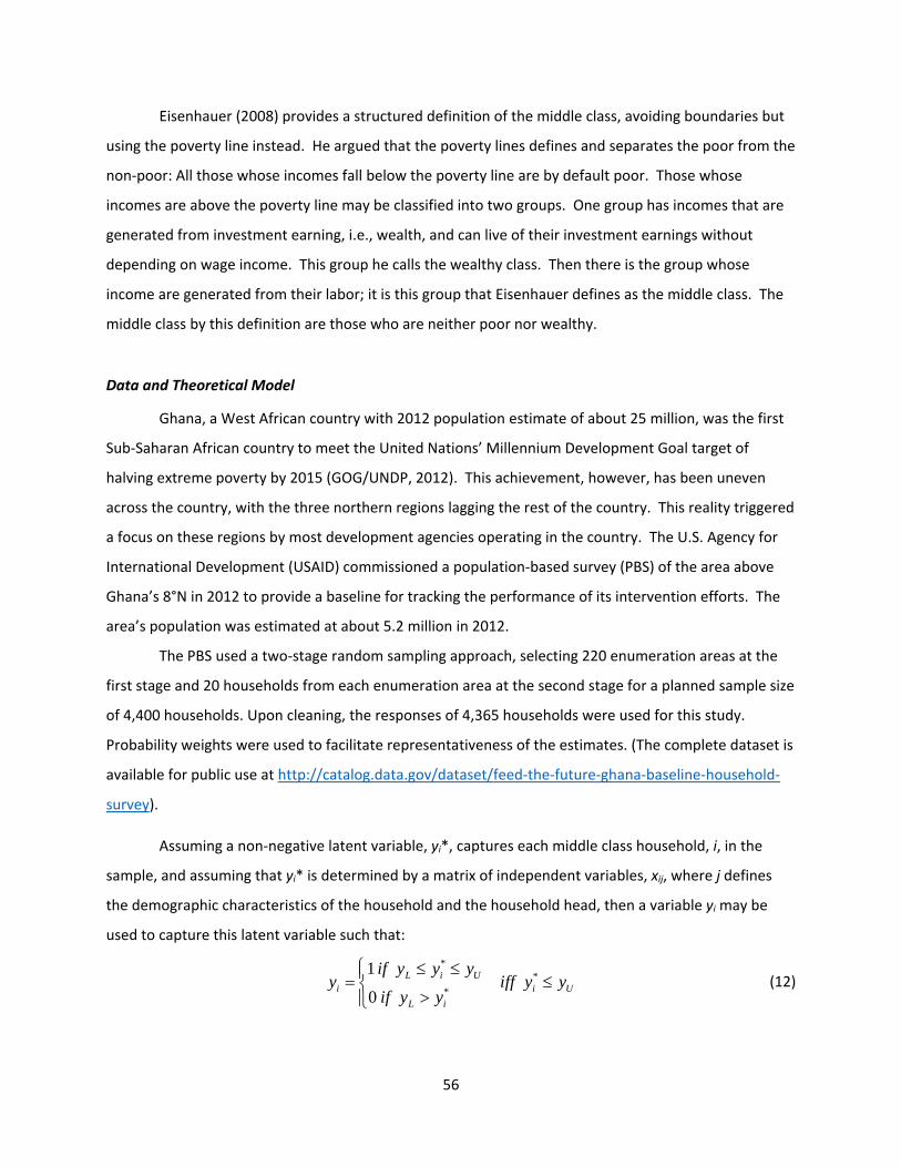
56
Eisenhauer (2008) provides a structured definition of the middle class, avoiding boundaries but
using the poverty line instead. He argued that the poverty lines defines and separates the poor from the
non‐poor: All those whose incomes fall below the poverty line are by default poor. Those whose
incomes are above the poverty line may be classified into two groups. One group has incomes that are
generated from investment earning, i.e., wealth, and can live of their investment earnings without
depending on wage income. This group he calls the wealthy class. Then there is the group whose
income are generated from their labor; it is this group that Eisenhauer defines as the middle class. The
middle class by this definition are those who are neither poor nor wealthy.
Data and Theoretical Model
Ghana, a West African country with 2012 population estimate of about 25 million, was the first
Sub‐Saharan African country to meet the United Nations’ Millennium Development Goal target of
halving extreme poverty by 2015 (GOG/UNDP, 2012). This achievement, however, has been uneven
across the country, with the three northern regions lagging the rest of the country. This reality triggered
a focus on these regions by most development agencies operating in the country. The U.S. Agency for
International Development (USAID) commissioned a population‐based survey (PBS) of the area above
Ghana’s 8°N in 2012 to provide a baseline for tracking the performance of its intervention efforts. The
area’s population was estimated at about 5.2 million in 2012.
The PBS used a two‐stage random sampling approach, selecting 220 enumeration areas at the
first stage and 20 households from each enumeration area at the second stage for a planned sample size
of 4,400 households. Upon cleaning, the responses of 4,365 households were used for this study.
Probability weights were used to facilitate representativeness of the estimates. (The complete dataset is
available for public use at http://catalog.data.gov/dataset/feed‐the‐future‐ghana‐baseline‐household‐
survey).
Assuming a non‐negative latent variable, yi*, captures each middle class household, i, in the
sample, and assuming that yi* is determined by a matrix of independent variables, xij, where j defines
the demographic characteristics of the household and the household head, then a variable yi may be
used to capture this latent variable such that:
**
*
1
0
L i Ui i U
L i
if y y yy iff y y
if y y
(12)
57
where yL and yU define AfDB’s lower and upper bounds of the middle‐income class respectively.
Equation (1) shows that yi takes on the value of 1 when yi* is greater than or equal to yL and lower than
or equal to yU. However, whenever yi* is greater than yL, yi is zero. The dataset on yi* is right‐
truncated in this analysis such that all observations where yi* is greater than yU are excluded from the
analysis, allowing a focus on households that meet the AfDB’s middle class definition. Structuring the
latent variable into a binary allows Equation (1) to be presented formally as:
0
00 ( )( 1) ( )1
j ji i
j ji i
X
i j ji i X
ey F X
e
(13)
where ρ defines the probability that yi = 1 and εi is the error term, assumed to normally distributed with
a zero mean and a variance of σ2, and β0 and βji are the estimated parameters for the independent
variables determining the probability that yi = 1.
The independent variables in Equation (2) include demographic characteristics of the household
head and the socio‐economic characteristics of the household. They are the household head’s gender,
age, education and marital status, the household size, the household’s locale and the proportion of
household expenditure allocated to food. Education is treated as a binary, where 0 implies the
household head has no formal education and 1 implies some formal education. The latter category is
very broad – from basic elementary education to university education. Marital status is also a binary,
where Married = 1 and Unmarried = 0 (and covers single, never married, separated, divorced and
widowed household heads). Households located in urban areas take on a locale value of 1 and those
located in rural areas take on a locale value of 0. For gender, female = 0 and male = 1. The remaining
two independent variables, age in years and proportion of total household expenditure spent on food in
percent, are continuous variables. We hypothesize positive coefficients for locale, gender, age,
education and marital status and negative coefficients for household size and food share.
Results and Discussion
The summary statistics of the study’s variables show that about 80.5 percent of respondent
household heads were male, 78.7 percent were married, 22.9 percent had some formal education and
their average age was about 44.2 years (Table 1). About 26.1 percent of households are located in
urban areas and the average household size is about 5.3 people, with an average food share of total
household expenditure of 63.3 percent. Households with per capita daily expenditure of between $2
and $20 accounted for 61.7 percent of the relevant sample. A further analysis reveals that rural

58
households are significantly larger by about one person (t = 9.78; P > |t| = 0.00) and have an average of
about 7 percent higher food shares (t = 10.87; P > |t| = 0.00). Similarly, households in which the head
has no formal education have about one person more on average than those in which the head has
some education and their food share was about 10.1 percent higher. Both differences are statistically
significant at the 1 percent level.
Table 2: Summary Statistics for Households with Per Capita Expenditures Not Exceeding $20/Day (N = 3,357)
Variable Mean S.E. [95% C.I.] Income Class (1 = Middle Class; 0 = Lower Class
61.7% 2.2% 57.3% 66.1%
Married (1 = Married; 0 = Not Married)
78.7% 1.2% 76.3% 81.1%
Locale (1 = Urban; 0 = Rural) 26.1% 3.4% 19.3% 32.9%
Gender (1 = Male; 0 = Female) 80.2% 1.3% 77.7% 82.8%Education (1 = Some Formal Education; 0 = No Formal Education)
22.9% 1.5% 19.9% 25.9%
Food Share 62.5% 0.6% 61.3% 63.7%Household Size 5.3 0.09 5.13 5.47Age (Years) 44.2 0.53 43.17 45.26
Table 2 shows the results of the logistic regression reporting the odd ratios. The model was
statistically significant at the 1 percent level, with an F(7,221) = 38.58. It shows that the odds of being in
the middle‐income class when married or when male are not statistically different from zero. That
means the probability of being in the middle‐income class was statistically not different for males and
females and for married and unmarried household heads in the study. Thus, the hypothesis that being
male or being married increased the odds of being in the middle‐income class cannot be accepted. On
the other hand, the odds of being in the middle‐income class when the household was in an urban locale
was approximately three times as high as the odds of being in the middle‐income class when the
household was in a rural locale. This difference was significant at the 1 percent level. The odds of being
in the middle‐income class when the household head had some formal education was about 2.4 times
higher than the odds of being in the middle‐income class when the household head had no formal
education, statistically significant at the 1 percent level. Thus, we cannot reject the hypothesis that
being in an urban area or having some education increased the odds of being in the middle‐income
class.

59
Table 3: Logistic Regression Odds Ratio Results (Dependent Variable Middle‐Income Class = 1 and Lower‐Income Class = 0)
Dependent Variable (Middle Class = 1)
Odds Ratio
Linearized Std.
Err. t P>t
[95% Confidence
Interval] Sig.
Marital Status Married 0.83 0.13 -1.17 0.25 0.61 1.13
Gender Male 1.09 0.13 0.70 0.48 0.86 1.39
Education Some (Basic - University) 2.35 0.34 5.99 0.00 1.78 3.11
***
Locale Urban 2.97 0.55 5.85 0.00 2.06 4.28 ***
Household Size 0.78 0.02 -12.37 0.00 0.75 0.81 ***Log of Age 0.70 0.12 -2.05 0.04 0.49 0.99 **Log of Food Share 1.45 0.21 2.52 0.01 1.08 1.94 ***Intercept 21.48 14.33 4.60 0.00 5.77 79.96
*** = 1% statistical significance; ** = 5% statistical significance
A percent change in the age of household heads reduced the odds of being in the middle‐
income class by about 30 percent while a percent change in food share of total household expenditures
increased the odds of being in the middle‐income class by about 45 percent. These two coefficients are
statistically significant at the 5 percent and 1 percent levels respectively. The age effect suggests that
the likelihood of being in the middle class declines with age of the household head, leading us to be
unable to accept the hypothesis that age increases the odds of being in the middle‐income class. This
result is not surprising as younger people are more likely to be more educated and have greater access
to higher incomes. The strong effect of education lends credence to this conclusion. On the other hand,
that increasing food share increases the odds of being in the middle class indicates that the households
in the study area are still below the income threshold that allows them to behave according to Engel’s
Law, i.e., a decline in their food share with increasing income. This suggests that the middle class in
Northern Ghana is vulnerable to adverse shocks to the economy, or at least it is not secure enough in its
food security to reduce its food share of its total expenditure.
The importance of this study is that it provides insights into what individuals can do to help
themselves migrate into the middle class from the lower‐income class and what governments and
development agencies may do to facilitate such a migration. We observe that five principal variables
influence the likelihood of being in the middle‐income class instead of the lower‐income class: age,

60
locale, education, household size and food share. Reiterating, one percent increase in family size is
expected to reduce the probability of being in the middle class by about 5 percent. However, getting
some education increases the probability of being the middle class by almost 16 percent and living in an
urban area instead of rural areal increases that probability by almost 20 percent.
Let us use the locale concept as a metaphor or representation for built infrastructure – good
roads, good schools, pipe borne water, and electricity. Looking at the results through such a lens would
suggest that availability (and accessibility) to built‐infrastructure increases the odds of being in the
middle‐income class by a significant factor. Built infrastructure is a public good, and therefore the
responsibility of government and government’s alone. Individuals, especially those already
economically challenged, cannot make much contribution in that effort. However, governments and
their development partners can choose to make direct investments into these infrastructures to provide
a platform from which individuals may act. For example, a good road connecting a rural community to
an urban community could motivate farmers in the rural communities along that road to make
investments in their production activities because they would have efficient access to markets. The
same road system, when combined with electricity and good schools, medical services and other
modern amenities, would improve the attractiveness of rural communities to a more diverse group of
people, reducing the embedded transaction costs associated with living in rural areas and increasing
opportunities. Avoiding or reducing these transaction costs and/or searching for opportunities explain
the high rural‐urban migration currently unfolding in many developing countries.
It is not enough for these infrastructures to be built; people must avail themselves to them in
practical and effective ways. Parents must make adequate investments in their children’s education,
supporting them and helping them take full advantage of schools and teachers in their communities.
But this is both individual and public responsibility and may be achieved through concerted, systematic
and enduring public education campaigns across rural communities. Helping people in these
communities understand the return on investments in education must be an integral part of public
policy. Development partners directing a significant portion of their budgets to the education effort –
both the infrastructure and the public awareness – would go a long way to facilitate the poverty
reduction and income enhancement objectives underscoring most of their work.
Recall that the proportion of respondents to the survey who had no formal education of any
kind was very high – about 78 percent. Sometimes, people who have not experienced a particular
benefit may not understand its value, and are therefore unable to justify making investments in it.
Without judgment and recognizing this as pure lack of information and knowledge, it may be beneficial

61
to achieving the long term objective of building and securing the middle class to undertake systematic
adult education. The purpose of this systematic adult education program is to help parents without
formal education achieve their own basic education credentials, allowing them to experience the value
of knowing, and in the process become education ambassadors. Celebrating parents’ success upon
completion of these adult education programs would go a long way to embed it into communities who
have not yet taken formal education for granted – in a good way. Thus, of the five variables influencing
the likelihood of being in the middle‐income class, individuals are responsible for their own education
and controlling their household size to match their economic capacity to fully utilize available
infrastructure. Governments are responsible for providing built infrastructure, supporting education
programs. There is nothing that can be done about age except helping younger people exploit
opportunities through encouragement in education. And when these are done, then people would take
care of the food share of their total expenditures and position themselves to eventually overcome the
income threshold that allows them to obey Engel’s Law.
Conclusion
There has been significant interest in the growth in the middle class in Sub‐Saharan Africa. This
paper sought to understand the factors that may explain migration into the middle class in a region that
has been designated as having a high poverty prevalence. We used the grouping defined by the African
Development Bank to define the middle class as those with average daily per capita household
expenditures between $2 and $20. The study showed that five factors contributed to explaining the
migration of an individual into the middle class instead of remaining in the lower income class:
education; whether they lived in a rural or urban area; age; food share of total expenditure; and
household size. We proposed a number of considerations for individuals and governments to help
facilitate a more robust middle class. Governments, with their development partners, must make
concerted efforts in building infrastructures in rural areas. This path was undertaken by the U.S.
government in the post‐WWII era with significant success in both rural productivity and economic
growth. The productivity in rural communities arise from the reduction in transaction costs associated
with living and working in rural communities that have no modern amenities. We also suggested that
individuals must take responsibility for the education of their children and themselves because it has a
significant effect on the probability of being in the middle class. Our results pointed to the value of
investing in providing adult education programs in rural communities may be a major pathway to
62
increasing their investment in their children’s education and choosing to reduce their household sizes.
These efforts all provide individual‐public‐private partnership opportunities.
References
Banerjee, A.V. and E. Duflo. “What is Middle Class about the Middle Classes around the World?” Journal of Economic Perspectives, 22(2008, 2): 3–28.
Birdsall, N., C. Graham and S. Pettinato. Stuck in Tunnel: Is Globalization Muddling the Middle? Working Paper 14, Washington, DC: Brookings Institution, 2000.
Chandy, L., N. Ledlie and V. Penciakova. The Final Countdown: Prospects for Ending Extreme Poverty by 2030, Washington, D.C.: Brookings Institution, 2013.
Development Initiatives. Investments to End Poverty: Real Money, Real Choices, Real Lives. Bristol, UK: Development Initiatives Ltd., 2013.
Easterly, W. “The Middle Class Consensus and Economic Development,” Journal of Economic Growth, 6(4, 2001): 317‐335.
Eisenhauer, J.G. “An Economic Definition of the Middle Class,” Forum for Social Economics, 37.2(2008): 103‐113.
Farag, M., A.K. Nandakumar, S.S. Wallack, G. Gaumer and D. Hodgkin. “Does Funding From Donors Displace Government Spending For Health In Developing Countries?” Health Affairs, 28(2005): 1045‐1055.
Government of Ghana (GOG) and UN Development Program (UNDP). 2010 Ghana Millennium Development Goals Report, Accra, Ghana: UNDP Ghana and NDPC/GOG, 2012.
Harvey, P. and J. Lind. Dependency and Humanitarian Relief ‐ A Critical Analysis. HPG Report ‐Humanitarian Policy Group, 2005.
Kharas, H. and J. Gertz. The New Global Middle Class: A Cross‐Over from West to East, in China's Emerging Middle Class: Beyond Economic Transformation" Cheng Li (Ed.), Washington, DC: Brookings Institution Press, 2010: 32‐54.
Ncube, M., C.L. Lufumpa and S. Kayizzi‐Mugerwa. The Middle of the Pyramid: Dynamics of the Middle Class in Africa. African Development Bank, Market Brief, April 20, 2011.
Ntale, C.L. Where Does Aid Money Really Go ‐‐ And What Is It Spent On? Special to CNN, Oct. 9, 2013. Available at http://www.cnn.com/2013/10/09/opinion/where‐does‐aid‐money‐really‐go/. Accessed Oct. 21, 2014.
Ouattara, B. “Foreign Aid, Public Savings Displacement and Aid Dependency in Cote d'Ivoire: An Aid Disaggregation Approach,” Oxford Development Studies, 35(2007, 1): 33‐46.
Perthel, D. “Engel’s Law Revisited,” International Statistical Review, 43(1975, 2): 211‐218.
Stewart, F. Technology Transfer for Development, in Science and technology: Lessons for Development Policy, Evenson, R.E. and G. Ranis (eds.), Boulder, CO: Westview Press, 1990: 301 ‐324.

63
The Economist. Poverty: Not Always with Us. www.economist.com/news/briefing/21578643‐world‐has‐astonishing‐chance‐take‐billion‐people‐out‐extreme‐poverty‐2030‐not/print. Accessed September 12, 2013.
Zereyesus, Y., K. Ross, V. Amanor‐Boadu and T. Dalton. Baseline Feed the Future Indicators for Ghana, 2012, Manhattan, KS: Kansas State University Press, 2014.
64
The Effect of Transaction Costs on Grain and Oilseed Farmers’ Market
Participation in Sub‐Saharan Africa: Recent Evidence from Northern
Ghana24
Agness Mzyece, Alex Shanoyan, Kara Ross, Yacob Zereyesus, and Vincent Amanor‐
Boadu
Department of Agricultural Economics
Kansas State University
Abstract
While agriculture offers a potential vehicle for the rural poor to escape poverty, the production
and marketing challenges faced by smallholder farmers make this potential difficult to tap. This study
examines factors influencing the intensity of market participation by maize, rice and soybean producers
in northern Ghana, where poverty is still endemic and likely exacerbated by fewer opportunities for
commercialization, such as access to markets. The analysis is based on the data from the agriculture
production survey conducted in 2013 and 2014 and the Population based Survey conducted in 2012 in
northern Ghana. Analysis is performed using the Double Hurdle approach to control for self‐selection
bias and provide unconditional effects of the variables on market participation. The results reveal a
greater participation for cash crop producing farmers than those producing a food crops, such as maize.
The results also show a positive relationship between transaction costs and intensity of participation
and suggest that farmers selling to aggregator‐type buyers and those having more buyers have a
propensity to sell more. These findings support market integration policy initiatives, such as building
sustainable and predictable market linkages and group marketing arrangements.
Key words: Market participation, intensity of market participation, small holder farmers,
Northern Ghana, Transaction costs
Introduction
A thriving agricultural sector is an important precondition for economic development in Africa in
general and in Sub‐Saharan Africa (SAA) in particular (Hakim Ben Hammouda 2006). In SSA, agriculture
accounts for 70 percent of employment and 35 percent of the region’s GDP (World Bank 2000). Over 80
percent of all rural households generate income and meet own food requirements through engaging in
24 An earlier draft of this paper was presented at the International Food and Agribusiness Management
Association 25th Annual Congress, June 2015, St. Paul, MN.

65
farm activities (IFAD 2011). Moreover, agriculture is the main source of livelihood for over three‐quarters
of the poor in SSA who live in rural areas (IFAD 2011). Consequently, strengthening the agricultural sector
by creating market linkages and promoting commercial agriculture is rising to the top of the agenda for
African countries in their poverty reduction strategies (Hakim Ben Hammouda 2006).
Market participation and commercial agriculture is widely seen as the key for unlocking economic
opportunities and enhancing incomes for smallholder farmers (Omiti 2009, Alene et al. 2008; Jagwe,
Machethe, and Ouma 2010). Research in Kenya and South Africa have shown a positive relationship
between the share of households’ agricultural output sold in the market and the level of production
efficiency and yields (Omiti 2009, Barrett 2008). Access to remunerative and reliable agricultural markets
can therefore enable farming households to improve their production systems and increase their farm
incomes. However, smallholder farmers in most SSA countries face numerous barriers to market access
and participation. Among such barriers are distance and poor road infrastructure, limited access to
resources and information, and associated high transaction costs for selling products in the market (Alene
et al. 2008).
High transaction costs have been argued to rank among the most important barriers for market
participation (Randela 2008, Alene et al., 2008). The economic literature defines transaction costs as the
combination of the observable and non‐observable costs associated with the exchange of goods and
services. (Coase 1937). Agribusiness and development literature have shown that transaction costs
associated with input procurement, buyer search, access to market information, and transporting goods
to market have a significant impact on producers’ market participation decisions (Goetz 1992, Key,
Sadoulet, and Janvry 2000; Randela 2008, Alene et al. 2008). This can be especially true for resource‐
constrained smallholder agricultural producers in developing countries. Numerous studies have found a
strong positive relationship between market participation and low levels of transaction costs especially
related to transport costs and information costs (Shepherd 1997, Heltber and Tarp 2002; Alene et al. 2008,
Ouma et al. 2010, Azam, Imai, and Gaiha 2012, Hlongwane 2014).
Recent studies of transaction cost and market participation in the context of SSA have largely
been carried out in east, central and southern African countries such as Kenya, Mozambique, South Africa,
and Ethiopia (Heltber and Tarp 2002, Barrett 2008, Alene et al. 2008, Omiti et al. 2009, Randela, Alemu,
and Groenewald 2008, Hlongwane, Ledwaba and Belete 2014). The body of market participation literature
in West African countries is relatively underdeveloped. Moreover, because of existing differences in
economic development, agricultural policies and practices, the findings from countries in east, central,
66
and southern Africa might not be readily generalizable to countries in West Africa. A recent report by the
African Union Commission (2012) shows that while the actual annual per capita GDP growth for West,
Central, East, and Southern regions was relatively similar, at 2.66%, 2.15%, 2.89% and 2.58% respectively,
the annual per capita GDP growth required to meet the MDG target on poverty reduction are significantly
different across these regions. They are 4.71%, 3.90%, 5.40% and 3.80%, respectively. The differences in
developmental stages in these regions highlight differences in resource endowments, government
policies on agriculture, inequality and levels of rural poverty.
This study attempts to provide more recent and direct empirical evidence of how transaction costs
affect market participation in northern Ghana. The northern region of Ghana is a good setting for this
study because of its poor access to markets, which is likely contributing to higher rates of rural poverty in
the region (Chamberlin, Xinshen and Shashi 2007). The analysis is based on the data from the agricultural
production survey of 527 farmers in Upper East, Upper West, Brong Ahafo and Northern Regions in Ghana.
The data comprise household characteristics, production characteristics as well as intricate market
behavioral variables such as type of major buyer the farmer sold to and how many types of buyers the
farmer sold to which very few market participation studies have managed to capture. It also allows a
comparison of market participation of maize, rice and soybean farmers.
Ghana is the first country in Sub‐Saharan Africa to meet the Millennium Development Goal target
of halving extreme poverty by 2015 (United Nations Development Programme 2012). However, poverty
is still endemic in the northern regions of the country. Three northern regions – Upper East, Upper West
and Northern Regions are home to more than half of the Ghana’s total population under extreme poverty
(Savannah Accelerated Development Authority 2010). While only 5% of Ghana’s population is considered
food insecure, the proportion of residents in the northern part of the country with food insecurity has
been estimated to be anywhere from double to seven times the national average (USAID|Ghana, 2012).
Similarly, the World Bank (2012) reports that while the number of the poor in southern Ghana declined
by 2.5 million, it increased by nearly 1 million in northern Ghana.
Higher rates of rural poverty in the northern regions of Ghana are likely exacerbated by factors
linked to fewer opportunities for intensifying and commercializing agriculture, such as poorer access to
input and output markets as well as credit and advisory services (Chamberlin, Xinshen and Shashi 2007).
The marketed share of farm products and the percentage of farmers who sell their produce tend to be
lowest in northern Ghana (Chamberlin, Xinshen and Shashi 2007). The average marketed surplus ratio of

67
agricultural produce in northern Ghana is 15% in the Upper East, 18% in the Upper West and 34% in
Northern region (Minot 2011) compared to an a national average of 33% (Musah 2014).
Crop production in the northern regions is overwhelming dominated by smallholder farmers in
areas that are considerably remote where barriers to market access are more pronounced. For example,
transaction costs along the maize chains may be equivalent to 80 percent of the farm gate price
(Chamberlin, Xinshen and Shashi 2007). Market‐driven assistance programs that link smallholder
producers to markets can therefore serve as important avenues for reducing food insecurity and poverty
in northern Ghana. Policy initiatives aimed at promoting sustainable development in northern Ghana such
as the Savannah Accelerated Development Authority (SADA) have already outlined and started
implementing strategies for improving market access and participation (Savannah Accelerated
Development Authority 2010). However, there is a scarcity of empirical evidence on how transaction costs
and other factors influence smallholder farmers’ market participation in the region.
Methods
Conceptual Framework
The theory underpinning this study is Barrett’s household non‐separable market participation
behavior model, which is based on utility maximization. The key features of this model are that a
household’s market access is not uniform because they face different transaction costs and that spatial
differences in cost of trade may result in geographical differences in marketing behavior (Barrett 2008).
These features induce households to rationally self‐select out or participate in the market. The basic
assumption of Barrett’s model is that a farm household faces a decision to maximize utility either as a net
buyer, net seller or autarkic, given a parametric market price for each crop. The choices facing the
household present specific transaction costs per unit sold. This model is appropriate for this study because
it uses two distinct layers of transaction costs, one that is household‐specific and another that is crop and
location‐specific to explore market participation, allowing market participation to vary by crop, household
and location (Barrett 2008). That is, given:
= agriculturalcommodity, = agriculturalcommodityfortrade, = householdspecificcharacteristicse. geducation, age,

68
= thehousehold’sassets, = publicgoodsandservices, suchasroads, gradesandstandards, extensionservicesetc, = off − farmearnings, = ( , ) − = , ( , ) = acropspecificproductiontechnology, = mapstheflowofservicesprovidedbyprivatelyheldquasi− fixed(andthusnontradable)assetse. gland, labor, livestock,machinery, = , = , ∗ =
The household optimization problem is: ( , ) Subject to a cash budget constraint = ∗ ( , ) + ℎ ∗ = − ( , , , , ) , ≤ ( , ) and = transaction costs.
The utility maximizing choice is determined by finding the optimal crop production and sales
choices and then identifying the market participation level that yields the maximum welfare (Key,
Sadoulet, and Janvry 2000, Stephens and Barrett 2006).
The household’s utility function is therefore:
( , , , , , , )
Data
The analysis is based on data from the agriculture production survey (APS) conducted in 2013 and
2014 in northern Ghana funded by the United States Agency for International Development (USAID). The
total sample includes 527 farmers in 51 enumeration areas across 25 districts in the Zone of Influence of
the USAID’s Feed the Future Initiative. The sample is representative of the population in northern Ghana.
It was achieved by utilizing a two‐stage stratified random sampling approach and developing probability
weights to account for differential probabilities of selection and non‐responses from the households.

69
The survey instrument was designed to collect detailed information on farmers’ production and
marketing characteristics. The production data were collected over the entire 2013 cropping season in
northern Ghana, from late June to mid‐November. The marketing data were collected during follow‐up
visits in January, February, and March of 2014 to capture accurate data on sales at harvest and after
storage. The crop production data mainly focused on the three focus crops of the Feed the Future
Initiative in northern Ghana: maize, rice, and soybeans. They include information on types of crop grown,
area planted, types of inputs used, and total output for each crop, as well as management practices and
production costs. The marketing data includes information on quantity sold, type of buyers, and price
received for each crop, as well as detailed information on marketing and transportation costs. The survey
also collected household demographic data.
The APS data is supplemented with additional data on relevant variables, such as age from the
baseline Population Based Survey (PBS) conducted in northern Ghana in 2012 and funded by Feed the
Future Initiative under USAID|Ghana. The baseline was from a sample size of 4600 drawn through a two‐
stage probability sampling approach. The households captured under the APS were largely captured under
the PBS such that triangulation of data from the APS onto the PBS data was possible.
Empirical Model
Given that sales are only observed for a subset of the sampled population because farmers who
did not sell their crop reported zero sales, the function estimated, i.e., proportion of output sold, on the
selected sample may not estimate the population, i.e., random sample, function (Heckman 1979) due to
self‐selection problems. Therefore, if the parameters were estimated by least squares, they would be
biased and inconsistent (Wooldridge 2009).
Other alternatives to modeling market participation are the Heckman sample selection model
(two step version18) used by Goetz (1992) Benfica, Tschirley, and Boughton (2006) Boughton et al. (2007).
The Tobit model proposed by Tobin (1958) as well as the double‐hurdle model originally proposed by
Cragg (1971). Heckman regression first estimates a probit model of market participation; then, in the
second step, one fits a regression of quantity traded by ordinary least squares (OLS), conditional on market
participation (Wooldridge 2003). It is designed for incidental truncation, where the zeros are unobserved
values (Ricker‐Gilbert, Jayne and Chirwa 2011). In this context however, a corner solution model is more
appropriate because the zeros in the data reflect farmers’ optimal choice rather than a missing value
(Reyes et al. 2012). The Tobit model could be used to model farmers’ marketing decisions but its major
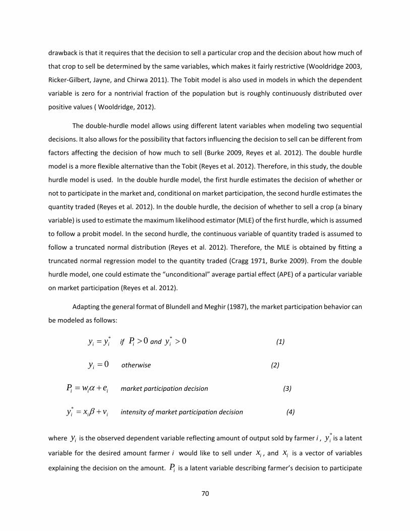
70
drawback is that it requires that the decision to sell a particular crop and the decision about how much of
that crop to sell be determined by the same variables, which makes it fairly restrictive (Wooldridge 2003,
Ricker‐Gilbert, Jayne, and Chirwa 2011). The Tobit model is also used in models in which the dependent
variable is zero for a nontrivial fraction of the population but is roughly continuously distributed over
positive values ( Wooldridge, 2012).
The double‐hurdle model allows using different latent variables when modeling two sequential
decisions. It also allows for the possibility that factors influencing the decision to sell can be different from
factors affecting the decision of how much to sell (Burke 2009, Reyes et al. 2012). The double hurdle
model is a more flexible alternative than the Tobit (Reyes et al. 2012). Therefore, in this study, the double
hurdle model is used. In the double hurdle model, the first hurdle estimates the decision of whether or
not to participate in the market and, conditional on market participation, the second hurdle estimates the
quantity traded (Reyes et al. 2012). In the double hurdle, the decision of whether to sell a crop (a binary
variable) is used to estimate the maximum likelihood estimator (MLE) of the first hurdle, which is assumed
to follow a probit model. In the second hurdle, the continuous variable of quantity traded is assumed to
follow a truncated normal distribution (Reyes et al. 2012). Therefore, the MLE is obtained by fitting a
truncated normal regression model to the quantity traded (Cragg 1971, Burke 2009). From the double
hurdle model, one could estimate the “unconditional” average partial effect (APE) of a particular variable
on market participation (Reyes et al. 2012).
Adapting the general format of Blundell and Meghir (1987), the market participation behavior can
be modeled as follows:
*ii yy if 0iP and 0* iy (1)
0iy otherwise (2)
iii ewP market participation decision (3)
iii vxy * intensity of market participation decision (4)
where iy is the observed dependent variable reflecting amount of output sold by farmer i , *iy is a latent
variable for the desired amount farmer i would like to sell under ix , and ix is a vector of variables
explaining the decision on the amount. iP is a latent variable describing farmer’s decision to participate

71
in the market under iw , and iw denotes a vector of variables explaining participation decision, ie and iv
are the respective regression errors. The probit model assumes that is independent of w and that e has the standard normal distribution (Wooldridge 2012).
Variable Description
In this study, market participation implies produce offered for sale and the use of purchased
inputs (Berhanu et al. 2010, Omiti 2009). Transaction costs are the observable and unobservable costs
associated with arranging and carrying out a transaction (Goetz 1992, Staal, Delgado, and Nicholson 1997).
Intensity of market participation is measured as the proportion of total output that is sold. Table 1
provides descriptive statistics on all variables used in this study.
The market participation decisions for each household are for the major crop produced by the
household; maize, rice or soybeans. Therefore, this marketing behavior is modeled as a function of
household characteristics, household assets, public goods and services, liquidity from net sales or off farm
income as well as additional market characteristics. However, due to data limitations, household assets
and liquidity are not included in this study. The variables used to capture household characteristics
include household size, Age (years), marital status, literacy and sex. These household characteristics can
affect search costs, negotiating skills (Barrett 2008). Public goods and services are defined as access to
institutional services and include access to credit and information. Production characteristics are
summarized as type of crop produced (maize, rice or soybeans) and output.
Marketing characteristics are measured by number of buyers, market distance, transport cost,
loading and offloading costs (load/offload costs), average price of produce faced by each household and
type of major buyer (whether aggregators, consumers, processors or other). Market distance is used as a
proxy for fixed transaction costs while transport and load/offload costs are used as a proxy for
proportional transaction costs. While transaction costs and price have often been included in most
previous market participation studies, number and major type of buyer have barely been studied. Farmers
who sell to bulky‐type buyers may sell more than those selling to individual household consumers who
buy enough for their consumption. In this study, it is also hypothesized that farmers who have more buyer
options may sell more than those with limited buyer options.
Berhanu and Moti (2010) and Randela (2008) modeled crop output market participation as a
function of household characteristics, resource endowment, access to market and roads, access to

72
institutional services, rainfall and household income from off‐farm and non‐farm sources. Household
characteristics include Age, Sex, Household Size, Marital status and Education. Resource endowment
includes land, animal draft power and assets. Access to markets includes distance to markets,
transportation cost and ownership of transport while access to institutional services includes credit and
market information. Omiti (2009) uses these same explanatory variables though not categorized as
Household characteristics, Resource endowments and access to markets and to institutional services.
Sebbata et al. (2014) include years of experience in farming and other sources of food in household
characteristics. Under assets, Sebbata et al. (2014) uses value of assets as well as monthly non‐farm
income. Under market access, he includes road condition and availability of village markets. Price and
time taken to walk to the field are other variables included. Hlongwane (2014) use gender, education,
distance to market, size of land under cultivation, access to market information, access to grants and
access to credit as the only factors affecting market participation.

73
Table 1: Summary Statistics on Variables used in Study
Variables Variable Description Mean Std. Error
Min Max
Household Characteristics Household size Continuous variable 10.65 5.64 2 53Age (years) Continuous variable 44.52 16.81 20 100Married (1 if yes) 0.91 0 1Literate (1 if yes) 0.02 0 1Male (1 if yes) 0.89 0 1Access to Institutional services
Access to credit (1 if yes) 0.37 0 1Access to information (1 if yes) 0.14 0 1Production Characteristics Farm Output (kg) Continuous variable 773.74 772.31 0 6000Rice (1 if yes) 0.12 0 1Soybeans (1 if yes) 0.06 0 1Marketing Characteristics Multiple buyers Continuous variable 0.53 0.908 0 4Market distance Continuous variable 0.4 3.41 0 65.25Transport cost Continuous variable 0.13 0.53 0 6loading & offloading cost Continuous variable 0.03 0.28 0 5Average Price (GHS/Kg) Continuous variable 0.12 0.17 0 1.05Sold to consumers (1 if yes) 0.15 0 1Sold to processors (1 if yes) 0.02 0 1Other buyers (1 if yes) 0.145 0 1
Empirical Results and Discussion
The factors found to be significant in influencing the decision to participate in the market at the
5% level include farm output (kg), access to information, access to credit and type of major crop produced
whether it was maize, rice or soybeans. The findings also show that factors significantly influencing the
intensity of market participation are access to credit, farm output (kg), type of major crop produced, major
buyer type (whether major buyer was consumers or aggregators), number of multiple buyers, transport
cost, loading and offloading costs as well as average price of produce.
As expected, farm output has a positive and significant (p = 0.00) impact on the decision to sell
and how much to sell. Farmers who produce more output are more likely to participate in the market and
sell more. Findings by Omiti (2009) also show a positive significant relationship between total farm output

74
and marketed produce. Access to credit and information has a positive impact on market participation
decision. This coincides with the findings by Hlongwane (2014) and Randela (2008) where access to credit
and market information were positively significant in affecting market participation of smallholder
farmers.
Table 2: Results of Probit Model on Market Participation
Variables Market Participation Intensity of Participation Coefficien
t Sig Robust
Std. Err. Coefficient Sig Robust
Std. Err. _Constant -0.830 *** 0.344 11.478 12.672Household Characteristics
Household size -0.021 * 0.012 -0.234 0.288Age (years) 0.005 0.004 0.020 0.127Other Marital status 0.092 0.270 -4.559 6.753Literacy level 0.403 0.248 4.548 5.582Male 0.005 0.250 9.678 7.407Access to Institutional services
Access to credit 0.276 * 0.146 3.963 3.744Access to information 0.753 *** 0.208 13.630 *** 5.128Production Characteristics
Farm Output (kg) 0.000 *** 0.000 -0.011 *** 0.004Rice 0.712 *** 0.223 10.416 * 5.497Soybeans 2.234 *** 0.498 26.901 *** 6.501Marketing Characteristics
Sold to consumers -25.888 *** 4.800Sold to processors -19.312 * 11.529Other buyers 16.595 ** 7.217Multiple buyers 14.934 *** 2.885Market distance 0.103 0.184Transport cost 4.823 ** 2.422loading & offloading cost 25.250 *** 7.636several sales visits -1.030 5.178Average Price (GHS/Kg) 44.493 *** 15.800sigma 21.430 *** 1.263*** = significant at 1%, ** = significant at 5% and * = significant at 10%

75
The results suggest that farmers whose major crop produced is a cash crop (rice or soybeans) are
more likely to participate in the market and also to participate at a greater intensity than farmers whose
major crop was a low value crop (maize). This makes intuitive sense, in that, production of cash crops is
mainly for purposes of selling whereas, production of maize, one of Ghana’s staples, is for both
consumption and sale. Maize has the highest per capita consumption and supply in Ghana (Ghana Ministry
of Food and Agriculture 2011). From this finding, it can be deduced that promotion of cash crop
production among smallholder farmers is one way of improving farmer’s market participation.
Following from the calculation of intensity of participation as a proportion of total output sold,
the results show that a negative significant relationship between farm output and intensity of
participation. This may be a merely formulae implication in which, with increase in farm output, the
differential increase in sales may not be as much as that in farm output resulting in the decrease in
proportion of output sold.
Concerning major buyer type, selling to consumers and other buyers is significant at 99% and 95%
confidence interval, respectively. Selling to Processors is significant at 90% confidence interval. Selling to
aggregators is the variable in the dummy variable trap. Farmers who mainly sell to consumers sell 25.9 Kg
less produce than those who sell to aggregators. This could be because aggregators generally buy large
quantities of produce for resale while consumers buy enough for their household consumption and hence
farmers selling to aggregators seem to be selling more than those selling to consumers are. Farmers who
sell to processors sell 19.3 Kg less produce compared to those who sell to aggregators. While processors
may also be bulky buyers, the number of processors buying from farmers could be only a handful
suggesting that some processors probably buy from other intermediaries such as aggregator.
Another mysterious buyer group is “other buyer types” consisting of the rest of the buyers besides
consumers, aggregators and processors. Farmers selling to other buyer types sell 16.6 Kg more than those
selling to aggregators. This finding shows the importance of carrying out a more thorough market analysis
to identify other important buyer types in northern Ghana who might be a significant part of building
strong value chains. Another interesting finding from the results is that farmers’ intensity of participation
increases as the number of buyer‐types increase. Farmers with more buyer‐types sell more as earlier
hypothesized. Additionally, as expected, Average price of produce was positive and significantly related
to intensity of participation at 95% confidence interval.
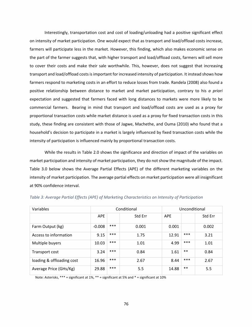
76
Interestingly, transportation cost and cost of loading/unloading had a positive significant effect
on intensity of market participation. One would expect that as transport and load/offload costs increase,
farmers will participate less in the market. However, this finding, which also makes economic sense on
the part of the farmer suggests that, with higher transport and load/offload costs, farmers will sell more
to cover their costs and make their sale worthwhile. This, however, does not suggest that increasing
transport and load/offload costs is important for increased intensity of participation. It instead shows how
farmers respond to marketing costs in an effort to reduce losses from trade. Randela (2008) also found a
positive relationship between distance to market and market participation, contrary to his a priori
expectation and suggested that farmers faced with long distances to markets were more likely to be
commercial farmers. Bearing in mind that transport and load/offload costs are used as a proxy for
proportional transaction costs while market distance is used as a proxy for fixed transaction costs in this
study, these finding are consistent with those of Jagwe, Machethe, and Ouma (2010) who found that a
household’s decision to participate in a market is largely influenced by fixed transaction costs while the
intensity of participation is influenced mainly by proportional transaction costs.
While the results in Table 2.0 shows the significance and direction of impact of the variables on
market participation and intensity of market participation, they do not show the magnitude of the impact.
Table 3.0 below shows the Average Partial Effects (APE) of the different marketing variables on the
intensity of market participation. The average partial effects on market participation were all insignificant
at 90% confidence interval.
Table 3: Average Partial Effects (APE) of Marketing Characteristics on Intensity of Participation
Variables Conditional Unconditional
APE Std Err APE Std Err
Farm Output (kg) ‐0.008 *** 0.001 0.001 0.002
Access to information 9.15 *** 1.75 12.91 *** 3.21
Multiple buyers 10.03 *** 1.01 4.99 *** 1.01
Transport cost 3.24 *** 0.84 1.61 ** 0.84
loading & offloading cost 16.96 *** 2.67 8.44 *** 2.67
Average Price (GHs/Kg) 29.88 *** 5.5 14.88 ** 5.5
Note: Asterisks, *** = significant at 1%, ** = significant at 5% and * = significant at 10%
77
The conditional APE shows the magnitude of the impact of the variable on intensity of
participation for farmers that participated in the market. For example, given that the farmer participated
in the market, a unit increase in price is associated with a 29.88 units increase in intensity of participation.
The Unconditional APE, on the other hand, shows the magnitude of impact of the variable on intensity of
participation for all farmers regardless of whether they participated in the market or not. Using price, for
example, a unit increase in price is associated with a 14.88 units increase in intensity of participation for
all farmers, irrespective of their participation decision. The APE shows that the variables with the highest
impact on intensity of participation are access to information, number of multiple buyers, loading and
offloading costs as well as price.
One of the limitations in this study was the difficult in including all relevant independent variables
in the models. While age and access to credit for the households in the data were obtained from the PBS,
data on off‐farm income, ownership of assets as well as ownership of transport which are other relevant
variables that could influence market participation could not be obtained. Future studies on market
participation can include these variables to observe their effect on participation.
Conclusion and Recommendations
The findings show that factors that significantly influence market participation include farm
output (kg), access to information, access to credit and type of major crop produced while factors that
significantly influence the intensity of participation are farm output (kg), buyer type, having multiple
buyers, crop produced, transport costs, loading and offloading costs and average price of produce.
These results reveal that farmers who sell to consumers sell less than those who sell to
aggregators‐type buyers in the market. The findings also show price and having multiple buyers are
positively and significantly related to intensity of market participation. These findings brings to light the
importance of value chain development in agricultural markets to increase farmers’ intensity of market
participation. Market integration initiatives such as value chain development, group marketing
arrangements can help to build strong and reliable linkages to markets thereby increasing market access
and participation opportunities for farmers. Policies that promote access to institutional services and
infrastructure development to reduce transaction costs can also be substantial in enhancing market
participation. Interventions in northern Ghana should focus on the establishment or expansion of high‐
value production‐market chains. Strategies to accomplish this goal can include out grower and contract

78
farming schemes, assistance for cooperatives, and an emphasis on coordinated support for input, credit,
and output markets.
References
Alene, Arega D., V M Manyong, G Omanya, H D Mignouna, M Bokanga, and G Odhiambo. 2008.
"Smallholder market participation under transactions costs: Maize supply and fertilizer demand
in Kenya." Food Policy.
Amankwah.K, L Klerkx, S J Oosting, O Sakyi‐Dawson, A J van der Zijpp, and D Millar. 2012. "Diagnosing
constraints to market participation of small ruminant producers in northern Ghana: An
innovation systems analysis ." NJAS‐ Wageningen Journal of Life Sciences 60– 63 37‐47.
Azam, M.S, K S Imai, and R Gaiha. 2012. "Agricultural Supply Response and Smallholders Market
Participation ‐ the Case of Cambodia." Research Institute for Economics and Business
Administration, Kobe University.
Barrett, Christopher B. 2008. "Smallholder market participation: Concepts and evidence from." Food
Policy 33 299–317.
Bellemare, Marc F., and Christopher B Barrett. 2006. "An Oredered Tobit Model Of Market
Participation:Evidence From Kenya And Ethiopia." Amer. J. Agr. Econ. 88(2 324–337 .
Benfica, R., D. Tschirley, and D. and Boughton. 2006. "Interlinked Transactions in Cash Cropping
Economies: The Determinants of Farmer Participation and Performance in the Zambezi River
Valley of Mozambique." 26th International Association of Agricultural Economists Conference.
Gold Coast: International Association of Agricultural Economists . 15p.
Berhanu, G, and J Moti. 2010. "Commercialization of Smallholders: Is Market Participation Enough?"
48th Agricultural Economists Association of South Africa (AEASA) Conference. Cape Town:
African Association of Agricultural Economists.
Boughton, D., D. Mather, C. B. Barrett, R. Benfica, D. Abdula, D. Tschirley, and B and Cunguara. 2007.
"Market Participation by Rural Households in a Low‐Income Country: An Asset‐Based Approach
Applied to Mozambique." Faith and Economics, Vol. 50 64‐101.
Burke, W. J. 2009. "Fitting and interpreting Cragg’s tobit alternative using Stata." The Stata Journal, Vol.
9 (4) 584‐592.
Cadot, Olivier, Laure Dutoit, and Marcelo Olarreaga. 2006. "How Costly Is It for Poor Farmers to Lift
Themselves Out of Subsistence?" World Bank Policy Research Working Paper 3881.
Coase, R.H. 1937. "The nature of the firm." Economica 4 386–405.
Cragg, J. 1971. "Some Statistical Models for Limited Dependent Variables with Application to the
Demand for Durable Goods." Econometrica, Vol. 39 (5) 829‐844.

79
Ghana Ministry of Food and Agriculture. 2011. Agric Facts and Figures. Ghana Ministry of Food and
Agriculture.
Goetz, S.J. 1992. "A Selectivity Model of Household Food Marketing Behavior in Sub‐Saharan Africa."
American Journal of Agricultural Economics 74, no. 2 444‐452.
Hakim Ben Hammouda, Stephen Karingi, Nassim Oulmane, Rémi Lang and Mustapha Sadni Jallab. 2006.
Can Market Access Help African Agriculture. African Trade Policy Centre.
Heckman.J. 1979. "Sample Selection Bias as a Specification Error." Econometrica, Vol. 47 (1) 153‐161.
Heltber.R, and F Tarp. 2002. "Agricultural supply response and poverty in Mozambiqu." Food Policy 27
103–124.
Hlongwane. J. J., Ledwaba. L. J., Belete. A. 2014. "Analyzing the Factors Affecting the Market
Participation of Maize Fatmers: A case study of small scale farmers in Greater Giyani Local
Municipality of the Mopani District, Limpopo Province." African Journal of Agricultural Research.
Holloway, G, C Nicholson, C Delgado, S Staal, and S Ehui. 2000. "Agroindustrialization through
institutional innovation: transactions costs, cooperatives and milk‐market development in the
east‐African Highlands." Agric. Econ. (23) 279–288.
International Fund for Agricultural Development. 2011. Rural Poverty Report. Rome: International Fund
for Agricultural Development.
Jagwe, John, Charles Machethe, and Emily Ouma. 2010. "Transaction costs and smallholder farmers’
participation in banana markets in the Great Lakes Region of Burundi, Rwanda and the
Democratic Republic of Congo." AfJARE Vol 6 No 1.
John Omiti, David Otieno, Timothy Nyanamba and Ellen Mc Cullough. 2009. "Factors influencing the
intensity of market participation by smallholder farmers: A case study of rural and peri‐urban
areas of Kenya ." Afjare.
Jordan Chamberlin, Xinshen Diao, Shashi Kolavalli, and Clemens Breisinger. 2007. Smallholder
Agriculture in Ghana. International Food Policy Research Institute .
Key, Nigel, Elisabeth Sadoulet, and Alain de Janvry. 2000. "Transactions Costs and Agricultural
Household Supply Response." Amer. J. Agr. Econ.
Mbanya.W. 2011. "Assessment of the Constraints in Soybean Production: A Case of Northern Region,
Ghana." Journal of Developments in Sustainable Agriculture, 6(2) 199‐214.
Minot, Nick. 2011. Innovative Policies on Increasing Access to Markets for High‐ Value Commodities and
Climate Change Mitigation. IFAD‐IFPRI Partnership Newsletter.
80
Musah, Abu Benjamin, Yaw Osei‐Asare Bonsu, and Wayo Seini. 2014. "Market Participation of
Smallholder Maize farmers in the Upper West region of Ghana." African Journal of Agricultural
Research 2427‐2435.
Ouma, E, J Jagwe, GO Aiko, and S Abele. 2010. "Determinants of Smallholder farmers' participation in
banana Markets in Central Africa: the role of transaction costs." Agric Econ 42(2) 111‐112.
Randela. R, Alemu. Z. G, Groenewald. J. A. 2008. "Factors enhancing market participation by small‐scale
cotton farmers." Agrekon Vol 47, No 4.
Reyes, Byron, Cynthia Donovan, Richard Bernsten, and Mywish Maredia . 2012. Market participation
and sale of potatoes by smallholder farmers in the central highlands of Angola: A Double Hurdle
approach. International Association of Agricultural Economists .
Ricker‐Gilbert, J., T. Jayne, and E. and Chirwa. 2011. "Subsidies and Crowding Out: A DoubleHurdle
Model of Fertilizer Demand in Malawi." American Journal of Agricultural Economics. Vol. 93(1)
26‐42.
Savannah Accelerated Development Authority. 2010. Savannah Accelerated Development Authority
Strategy and Work Plan. Savannah Accelerated Development Authority.
Savannah Accelerated Development Authority. 2010. Savannah Accelerated Development Authority
Strategy and Work Plan 2010 ‐ 2030. Savannah Accelerated Development Authority.
Sebbata, C, J Mugisha, E Katungi, A Kashaaru, and Kyomugi. 2014. "Smallholder Farmers’ Decision and
Level of Participation in the Potato Market in Uganda." Scientific Research Publishing Inc.
Shepherd.A. 1997. "Market Information Services: Theory and Practice." Food and Agriculture
Organization.
Staal.C, Delgado.C, and Nicholson.C. 1997. "Smallholder dairying under transactions costs in East Africa."
World Develop. 25 (5) 779–794.
Stephens, E.C, and C B Barrett. 2006. "Incomplete credit markets and commodity marketing behavior."
Cornell University Working Paper.
Stephens, Emma C., and Christopher B. Barrett. 2011. "Incomplete Credit Markets and Commodity
Marketing Behaviour." Journal of Agricultural Economics, Vol. 62, No. 1 1–24.
Tobin, J. 1958. "Estimation of Relationships for Limited Dependent Variables." Econometrica, Vol. 26 (1)
24‐36.
United Nations Development Programme. 2012. 2010 Ghana Millenium Development Goals Report.
United Nations Development Programme.
Wood, Tara N. 2013. Agricultural Development in the Northern Savannah of Ghana. University of
Nebraska‐ Lincoln.

81
Wooldridge, Jeffrey M. 2012. Introductory Econometrics: A Modern Approach. Ohio: South‐Western .
Wooldridge, M.J. 2009. Sample selection and missing data. Michigan: Michigan State University.
Wooldridge, M.J. 2003. Introductory Econometrics: A Modern Approach. 2nd ed. SouthWestern
Publisher.
World Bank. 2000. Can Africa Claim the 21st Centuary. Washington DC: World Bank.
Zanello.G. 2011. "Does the use of mobile phones reduce transactions costs and enhance participation in
agricultural markets? Household evidence from northern Ghana." CSAE Conference
2011:Economic Development in Africa, Vol. 44 1–23.
World Bank. 2012. Ghana. Retrieved from http://data.worldbank.org/country/ghana. USAID|Ghana. RFP
USAID/Ghana SOL‐641‐12‐000005. September 2012.

82
Reducing Gender Differences in Agricultural Performance in Northern
Ghana
Elizabeth Gutierrez, Kara Ross, Yacob A. Zereyesus, Aleksan Shanoyan, and
Vincent Amanor‐Boadu
Department of Agricultural Economics
Kansas State University
Abstract
Even though women are involved in a variety of agricultural activities, they have limited access to
resources and have restricted decision‐making power. These limitations and restrictions are likely to have
a significant effect on women’s performance levels compared to men. The present research measures the
gender‐based performance differences and identifies the factors that influence these differences among
smallholder farmers in northern Ghana. Data used in this study are from the Agriculture Production
Survey (APS) focusing on the 2013‐2014 cropping season. The study uses the Oaxaca‐Blinder
decomposition method to measure and decompose the gender performance gap in two parts: the
explained and the unexplained parts. Gross margins are used to measure farmer performance. The
explained part is attributed to differences in the explanatory variables, and the unexplained part is
associated with discrimination or omitted variables. Results from the study indicate there is a gender gap
between male and female smallholder farmers with male farmers outperforming females two to one.
Land area had the largest significant impact on the explained part of the gender gap, followed by
agrochemical use. The explained part of the decomposition model accounted for 47 percent of the gender
gap, and the remaining 53 percent is associated with the unexplained part. The larger unexplained part
suggests that developing programs to establish equality among male and female smallholder producers
in terms of access to resources will not close the gender gap. Further research into factors affecting the
gender gap in economic performance in agricultural activities is warranted.
Key words: Gender differentials, agricultural production activities, gross margins, Oaxaca Blinder
Decomposition, Ghana
83
Introduction
Sub‐Saharan Africa has one of the highest female labor‐force participation rates worldwide. In the
agriculture sector, women represent on average 50 percent of the labor force in Sub‐Saharan Africa (FAO,
2011) with women represent 36 percent of the labor force in Cote d’Ivoire, and in Niger, Lesotho,
Mozambique, and Sierra Leone, each country has over 60 percent of female labor force participation rate
(FAO, 2011). Despite the fact women provide a significant level of participation, agriculture is a sector
where noticeable gender differentials exist. Aguilar et al (2014) found that the productivity level of male
land managers in Ethiopia are 23.4 percent higher than their female counterparts, and these differences
are attributable to land manager characteristics, land attributes, and unequal access to resources. In a
study conducted by Oseni et al (2014), male plot managers in northern Nigeria were found to have a
higher productivity level than female plot managers by 28 percent. Although the gender difference in
Uganda is lower than in Nigeria, a significant gender gap in productivity still exists of 17.5 percent due to
observed parcel characteristics, unobserved household, community, season, and farmer characteristics
(Ali et al, 2015).
Sub‐Saharan women play a central role not just in agriculture but in domestic activities. In their
households, women are the primary caregivers and are more concerned about providing the necessities
of their children’s health and well‐being (Duflo, 2000). Most of these domestic activities are unpaid
activities (FAO, 2011). In Kenya, women perform more activities than men not only in the field but also
at home. In the household, women are responsible for preparing food, caring for their children and
gathering firewood and water, and in the field women perform most of the cropping activities and help
to raise the livestock (Saito et al, 1994). Rural women in Zambia contribute 18 percent more labor than
men in agricultural production activities (Mwila, 1981) and on average, 50 percent more hours per day
than men (Saito et al. 1994).
Despite the importance of women’s participation in the agricultural sector, unequal access to
resources and inputs exist between men and women in many countries in Sub‐Saharan Africa. The gender
differentials are thought to be attributed to the lack of limited access to resources, such as land, livestock,
technology, and financial, and lack of training and education. The challenges associated with the lack of
access to resources and low levels of human capital are thought to affect all aspects of women’s lives.
Although, women may lack of resources as land and inputs of agricultural production in Sub‐Saharan
Africa, there is empirical evidence suggesting that females are, or are almost as, technically efficient as
men (Adesina et al, 1997; Kinkingnimhoun‐Medagbe et al, 2010). In some cases, women were more
technically efficient than their counterpart males. In a study conducted in Osun State, Nigeria, Oladeebo

84
(2007) estimated a stochastic frontier production and found that female rice farmers had a higher
technical efficiency mean index (0.904) than men (0.897), this implies that female rice farmers are more
efficient with a 9.6 percent below of the maximum feasible output in contrast with the 10.3 percent in
men case. These results suggest that differential in gender productivity is not due to lack of knowledge in
management of inputs in the crop production, indeed given the lack of resources women have had, they
are producing the best they can.
Given the importance of women in agriculture, the gender‐specific constraints that poor female
smallholder farmers encounter has garnered a lot of attention in recent years from development
practitioners, activists and agribusiness practitioner. Many of the development and agribusiness
intervention programs have shifted focus to targeting areas in northern Ghana. Northern Ghana
represent more than half of the total land surface of Ghana, but its contribution to economic growth is
far below that of southern Ghana (World Bank, 2004). A significant portion of the population in northern
Ghana relies on agriculture for its livelihood; however, this is a challenging region for agriculture
production due to adverse conditions of poor soils, and unpredictable rains (Dickson, 1968). Compared to
southern Ghana, northern Ghana presents higher rates of malnutrition and poverty, particularly in the
rural areas. A number of these initiatives are focused on improving the livelihoods of smallholder farmers
by increasing their productivity, especially poor female smallholder farmers. For example, a key objective
of the United States Agency of International Development’s (USAID) Feed the Future Initiative in northern
Ghana is to promote inclusive agriculture sector growth by “increasing agriculture production and the
incomes of both men and women who rely on agriculture for their livelihoods” (USAID 2011).
Northern Ghana’s large agricultural sector and the significant amount of attention received from
the development community make it an interesting and relevant country to examine in regards to
improving agricultural productivity and performance to reduce poverty and food insecurity. The aim of
this study is to examine and measure the gender‐based performance differences within the agriculture
sector in northern Ghana, using household level data from the Agriculture Production Survey (APS) of
2013‐2014. This study also identifies the factors that influence performance levels of smallholder farmers
in northern Ghana. For the purpose of this study, farmer performance is measured by gross margins,
which provide a good estimate of how profitable a farmer is. An analysis that identifies the factors that
influence the gender‐based performance gaps may have valuable policy implications for northern Ghana.
Results from this study will lead to a better understanding of the situation in northern Ghana for women
participating in the agriculture sector and will help guide future research priorities to develop informed
policy interventions aimed at closing the gender gap by increasing women’s human capital and resources

85
promote agricultural growth, higher income for women, and better food security for all (Quisumbing
1995). Also, results from this type of analysis may also be applied to other countries experiencing similar
situations in their agricultural sector and have a high prevalence of poverty and food insecurity.
Data
The dataset used in this study is from the USAID funded APS conducted in northern Ghana (Upper
West, Upper East, Northern, and parts of Brong‐Ahafo) during the entire 2013 cropping season, from later
June to mid‐November. Follow‐up visits were conducted in January, February and March 2014 to collect
sales data from respondents. The survey is part of the USAID Ghana’s Feed the Future Initiative, which is
aimed at helping northern Ghana address root causes of hunger and poverty specific to their individual
and unique circumstances through the transformation of agricultural production and improvement in
health and nutrition.
Figure 13. Map of the regions of Ghana
Source: Adapted from Golbez (2005)
The survey questionnaire focused on crop production and marketing data for three main crops in
northern Ghana: maize, rice, and soybeans. Data collected included household demographics, production
costs, and marketing and sales cost. A two‐stage stratified random sampling design was used in this
survey. In total, data were collected from 527 smallholder farmers across 25 districts in the studied area.
For the purpose of this study, data incorporated into the models included labor and non‐labor inputs, field
characteristics, and smallholder farmer characteristics.
Method
86
The Oaxaca‐Blinder decomposition method is a tool often used to study group outcomes. The
decomposition method has been used widely in the field of labor economics. Oaxaca (1973) and Blinder
(1973) made this analysis technique popular through the decomposition of wage earning gaps and the
estimation of discrimination in gender earning differentials. In recent years, this decomposition method
has been extended into the analysis of ethnic earnings differentials, public/private sector earning
differentials, earning differentials by socioeconomic background, testing effectiveness of jobs training
programs and other applications. Also, this decomposition method has been applied to other fields, such
as sociology for the analysis of social issues including education (Barrera‐Osorio et al. 2011).
The Oaxaca‐Blinder (Blinder 1973, Oaxaca 1973) decomposition method allows the researcher to
calculate the mean differences of a variable of interest and to identify the contribution of each factor of
production to the difference between the groups. This decomposition method divides the mean
differential between the explained, i.e., endowment effect, and unexplained components, i.e., structural
effect. The explained component is the part of the differential in farmers’ performance due to group
differences in the explanatory variables while the unexplained component is due to discrimination or
omitted predictors.
Recently, the decomposition method has be used to analyze gender differentials in agricultural
productivity. Aguilar et al. (2014) employ the Oaxaca‐Blinder technique to estimate differences in
agricultural productivity between female and male farm managers in Ethiopia and to identify the main
drivers of the gender differential. Oseni et al. (2014) conducted a study using the decomposition method
to analyze differences in productivity between male and female plot managers in northern and southern
Nigeria.
The conceptual model used in this study is based on a performance function. Farmer performance
is thought to be a function of demographic, production and input variables. Gross margin is the
dependent variable used to measure smallholder farmer performance in northern Ghana. Gross margin
captures the difference between revenue and variable cost of production, and it is measured in Ghanaian
cedis (GHS). It is considered a good indicator of performance because (1) it captures the efficient
management of production factors; and (2) the fixed costs are minimal in northern Ghana case. The
performance function is represented as:
= + + + + +
where X, Y and Z are vectors representing the demographic, production, and input variables,
respectively. The gender variable represents the gender of the famers where female farmers are coded

87
as 0 and males are 1. This is also the group defining variable. The demographic variables included in the
model are education and child dependency ratio. Education is a binary variable where 1 indicates that the
farmer has some level of formal education (primary, secondary or tertiary level) and 0 if otherwise. Child
dependency ratio represents the ratio of children to adults, both male and female, in the household. The
Y vector of production variables provides information on agricultural practices used in the crop production
including the number of crops produced per household per season and the decision to intercrop. The
intercropping decision variable is a binary variable representing the decision to concurrently grow two or
more crops in the same field plot where 1 indicates the decision to intercrop and 0 for monocropping. The
input variables in the Z vector capture the inputs and resources used by the smallholder farmers and
include the following inputs and resources: agrochemical, fertilizer, labor, land, seed type, and tractor
use. Agrochemical variable represents the percentage of agrochemical applied at the household level.
This variable is the ratio of the total kilograms of chemical to the number of plots at household level.
Fertilizer variable represents how much fertilizer has been applied to the plots of the household level and
it is represented in percentage. Fertilizer is the ratio of the total kilograms of fertilizer to the number of
plots at household level. Labor and land area are transformed into logarithmic form to normalize these
variables in order to align the values to a normal distribution. Labor log is the natural logarithm of the sum
number of hired, communal, and family labor hours worked during the season, and land log is the natural
logarithm of area measured in acres used in the growing season, both at the household level. Type of seed
is a binary variable where 1 represents the farmer’s decision to use improved seed and 0 otherwise.
Tractor service is another binary variable, in which 1 denotes the use of a tractor in the agricultural related
activities.
Given the variables are grouped by vectors X, Y, and Z to denote demographics, production and
inputs variables, respectively, it was estimated models with sequence of the vectors. To estimate sequent
the model with the vectors allow us to check robustness and significance of the GENDER coefficient.
Following Sandy and Duncan (2010), this decomposition technique can be separated in two
equations, one for female smallholder farmers and other for male smallholder farmers. These equations
can be illustrated as: = + (1) = + (2) where α denotes the intercept parameter, β is the slope parameter and K is a vector containing the
predictors.

88
The gap or difference in performance between these two groups can set up as (Gross Marginmales‐
Gross Marginfemales). Also, this difference can be detailed as:
− = ∆ ( ) (3a) ∆ = − + − + ( − ) (3b)
This outcome difference equation can be decomposed into two components: ( − ) (4)
− + − (5)
Equation 4 is the “explained” outcome differential indicating how much of the gender gap in gross
margin is due to differences in the predictors. It is based on the portion of the Oaxaca‐Blinder outcome
due to differences in average characteristics between male and female smallholders in northern Ghana.
The remaining values are the intercept term and the slope coefficient term, which represent the
“unexplained part”. It is important to note that the unexplained part can be attributed to discrimination
and unobserved variables, which makes interpretation of this part difficult.
This research provides an analysis of the explained portion of the gap through the Oaxaca‐Blinder
detailed decomposition approach. Results of the unexplained detailed portion are provided in the
Appendix 1. This model was estimated following the method developed by Jann (2008) for the STATA®
software package.
Results and Discussion
Table 1 provides summary statistics of these variables for female smallholder farmers and male
smallholder farmers. From the APS data, this study captures data from 506 respondents of which 454
observations are male respondents and 52 observation are female respondents. Differences in gross
margin, child dependency ratio, log land area, agrochemical, and tractor service were found to be
statistically significant at the 1 percent level and differences in fertilizer were found statistically significant
at the 5 percent.
Based on our results, male smallholder farmers’ gross margin is larger than female farmers by
476.40 GHS. Moving to Vector X, the majority of men and women have little to no education, and female
farmers have, on average, a higher children dependency than male, this means that female farmers are
in charge of more children than their counterpart. Variables contained in Vector Y indicates that overall

89
farmers choose to not intercrop and to produce one crop by production cycle. In Vector Z, land area in
males is higher than females, this could indicates that females have less land area to produce than males.
Although, male farmers use 17 percent more agrochemical than females in the crop production. Regarding
to type of seed both groups use traditional seed and male farmers in northern Ghana are more likely to
use a mechanical tractor in managing their fields than their female farmers.
Table 2 provides a robustness check with control for demographic variables (Vector X) and
production variables (Vector Y). Estimates from the least squares estimates for the pooled sample and
each farmer group are presented in Table 3. In the pooled model, education has a positive effect on farmer
performance and was found to be statistically significant. If farmers receive some formal educational
training, this will have a positive impact on their economic performance of their agricultural activities.
Land and agrochemicals are inputs that positively affect farmers’ performance. The number of crops
produced was found to have a significant and positive impact on gross margin suggesting that
diversification is economically beneficial for the farmer.
When comparing the male farmer model to the pooled model, the same variables are statistically
significant with positive signs and similar magnitudes in both models. The results suggest that male
farmers can increase their gross margin if they have access to more land, use more agrochemical, have a
diverse crop portfolio, and have some level of formal educational training. This same similarities were
not present in female model. In all three models ‐ pooled, male and female models ‐ the number of crops
produced is statistically significant but not at the same significance level. Also, the coefficient for this
variable is larger in the female model compared to the other two models indicating that the decision to
grow more than one crop during the cropping season has a higher impact on female farmers than male
farmers. For female farmers, labor is significant with a negative sign. Thus, increasing labor by one percent
decreases female farmers’ gross margin. Female farmers utilizing tractors for crop production activities
has a significant and positive effect on their economic performance. Agrochemical use has a significant
and negative effect on female farmers’ performance. This results is counter to our expectation and the
relationship found in the male and pooled models. A possible explanation for this result may be that
females have already optimized agrochemicals application on their fields and additional agrochemical
application would have adverse effect on their crops or would add no benefit. Both outcomes would
negatively impact female farmers’ gross margins either by reducing revenue or increasing variable costs.

90
Decomposition Gender Differentials
The Oaxaca‐Blinder model decompose differences in performance of two specific groups: males
and females. Table 3 is structured into two sections. The first part Mean Gender Differential provides the
estimates of gross margin for the two groups of this study. Male gross margin for men and female were
found statistically significant. The difference in gross margin is the difference between male and female
gross margin, and it is statistically significant. The aggregate decomposition results indicate that mean
gross margin for male farmers is 482.54 GHS higher than for female farmers. This results in 50.71 percent
in gender performance gap. The second part, aggregate decomposition presents the endowment effect
and male advantage (structural effect), both were found to be statistically significant. The gender
performance gap of 50.71 percent consists of two components: the explained and unexplained parts. The
explained part accounts for 47 percent of the 51 percent gap and the remaining percentage, i.e., 53
percent, is associated with the unexplained part. Translating these percentages into a monetary amount
indicates that 228.72 GHS of the 482.54 GHS gross margin gap is due to the differences in the average
characteristics of male and females smallholder farmers. The remaining 253.82 GHS represents the
unexplained part and can be attributed to omitted variables. Thus, the explained part was found to be
smaller than the unexplained part. This result suggests that even if men and women have equal
production conditions and access to the same resources, significant differences in their gross margin
earnings will continue to be exist.
Detailed Decomposition
In this study, the Oaxaca‐Blinder model identifies factors that influence performance levels of
smallholders in northern Ghana. Table 4 provides the results of the detailed decomposition analysis, which
consists of the explained and the unexplained components. The unexplained component is separated into
the male structural advantage and the female structural disadvantage models (Appendix 1). For
interpretation of the results, it is important to note that factors with positive coefficients expand the
gender gap while negative coefficients reduced the gap. In the explained portion of the model, land and
agrochemicals are the two significant variables, and they both contribute to widening the gender gap. Of
the two variables, land area has the largest impact on the gap.
The contribution of land and agrochemicals to the explained part of the gender gap and the overall
gender gap is calculated by dividing the variables’ coefficients by the total explained part of 228.72 GHS
and by dividing by the overall difference in gross margin of 482.54 GHS. Land area contributes 57 percent

91
of the total explained part and 27 percent of the overall gender gap. Agrochemical accounts for 24 percent
of the explained part and 11 percent of the overall gender gap.
Conclusions
This research studied the gender differences in agricultural performance in northern Ghana using
a data set from the USAID funded APS 2013‐2014. The aim of this study was to determine the gender‐
based performance differences in agricultural activities and identify factors that influence performance
levels. Evidence presented in this study confirmed the existence of gender gap in performance by
smallholder farmers as measured by gross margins. This gap suggested that female farmers’ gross margin
is 51 percent lower than male farmers. Agrochemical use and land area were the two factors that
contributed to the explained part of the gender gap. Both of these factors contributed to widening the
overall gap between male and female smallholder farmers with land area having the largest impact. When
examining the male and female models separately, an increase in agrochemical use did not improve
female smallholder famers’ performance but it did improve males’ performance. This results suggested
that programs developed to increase farmers’ access to and adoption of agrochemicals would not have a
positive effect on women’s gross margins, and thus, would not help to close the gender gap.
With regard to the detailed decomposition analysis, the unexplained part was larger than the
explained part. Therefore, regardless of program interventions to provide men and women with equal
access to resources and production conditions, gender differentials between male and female smallholder
farmers will persist. Because of data limitations in this study, it is likely that important factors contributing
to the gender gap were not included in this research. Further research into other key factors contributing
to this gender differential is needed to fully understand what programs can be developed for smallholder
farmers in northern Ghana to effectively close the gender gap.
References
Adesina, A. A., & Djato, K. K. (1997). “Relative efficiency of women as farm managers: Profit function
analysis in Cote d'ivoire”. Agricultural Economics (Amsterdam, Netherlands) Agricultural
Economics : The Journal of the International Association of Agricultural Economists, 16(1), 47‐53.
Aguilar, A., Carranza, E., Goldstein, M., Kilic, T., Oseni, G. 2014. “Decomposition of gender differentials in
agricultural productivity in Ethiopia”. Policy Research working paper; no. WPS 6764.
Washington, DC: World Bank Group. Retrieved from
http://documents.worldbank.org/curated/en/2014/01/18894327/decomposition‐gender‐
differentials‐agricultural‐productivity‐ethiopia.

92
Ali, D., Bowen, D., Deininger, K., Duponchel, M. 2015. “Investigating the Gender Gap in Agricultural
Productivity: Evidence from Uganda”. World Bank, Washington, DC. Retrieved from
https://openknowledge.worldbank.org/handle/10986/21994 License: CC BY 3.0 IGO.”
Barrera‐Osorio, F., Garcia‐Moreno, V., Patrinos, H., Porta, E. 2011. “Using the Oaxaca‐Blinder
Decomposition Technique to Analyze Learning Outcomes Changes over Time: An Application to
Indonesia’s Results in PISA Mathematics”. World Bank Policy Research Working Paper 5584.
Blinder, A.S. 1973. “Wage discrimination: reduced‐form and structural estimates”. Journal
of Human Resources. 8:436‐55
Dickson, K. B. 1968. “Background to the Problem of Economic Development in Northern Ghana”. Annals
of the Association of American Geographers. 58(4): 686‐696.
Duflo, Esther. 2000. Grandmothers and Granddaughters: Old Age Pension and Intra‐household
Allocation in South Africa. 8061.
(FAO) Food and Agriculture Organization of the United Nations. 2011. The State of Food and Agriculture
2010‐11. Women in Agriculture: Closing the gender gap for development. Retrieved on May 27,
2014 http://www.fao.org/docrep/013/i2050e/i2050e00.htm.
Jann, B. 2008. “A Stata implementation of the Blinder‐Oaxaca decomposition”. Stata Journal. 8: 453‐79.
Kinkingninhoun‐Medagbe, F. M., Diagne, A., Simtowe, F., Agboh‐Noameshie, A. R., & Adegbola, P. Y.
(2010). Gender discrimination and its impact on income, productivity, and technical efficiency:
Evidence from Benin. Agriculture and Human Values, 27(1), 57‐69.
Mwila, H. 1981. An Observation of some of the Major Socio−Economic Characteris cs of Rural
Households in Mubanga, Chinsala District, University of Zambia, Rural Development Studies.
Nyanteg, V.K., and S. Asuming‐Brempong. 2003. The Role of Agriculture in Food Security in Ghana. A
paper presented at Roles of Agriculture Project International Conference 20‐22 October, 2003
Rome, Italy. Organized by Agricultural and Development Economics Division (ESA) Food and
Agriculture Organization of the United Nations.
Oladeebo, J. O. (2007). Technical efficiency of men and women upland rice farmers in osun state,
Nigeria. Journal of Human Ecology, 22(2), 93.
Oaxaca, R. 1973. “Male‐female wage differentials in urban labor markets”. International Economic
Review 14: 693‐709.
Oseni, G., P. Corral, M. Goldstein, and P. Winters. 2014. “Explaining gender differentials in agricultural
production in Nigeria”. Policy Research working paper; no. WPS 6809. Washington, DC: World
Bank Group. Retrieved from

93
http://documents.worldbank.org/curated/en/2014/03/19269811/explaining‐gender‐
differentials‐agricultural‐production‐nigeria.
Quisumbing, A. R., L. R. Brown, H. Sims Feldstein, L. Haddad, and C. Pena. 1995. Women: The Key to
Food Security. International Food Policy Research Institute.
Saito, K.A., H. Makonnen, and D. Spurling. 1994. Raising the productivity of women farmers in sub‐
Saharan Africa. World Bank Discussion Papers Vol (230).
Sandy, J., and K. Duncan. (2010). Examining the achievement test score gap between urban and
suburban students. Education Economics, 18(3), 297‐315. doi:10.1080/09645290903465713.
(USAID) United States Agency of International Development’s Feed the Future. 2011Inclusive Agriculture
Sector Growth. Washington, DC. Retrieved on November 30, 2014 from
http://www.feedthefuture.gov/ftf.
World Bank. 2004. Bridging the North South Divide in Ghana. Washington, DC: World Bank. Retrieved
from https://openknowledge.worldbank.org/handle/10986/9053.

94
Table 4. Summary Statistics of the Variables Used in the Model
Variables Description
Female Male
Differences Mean
Standard Deviation
Mean Standard Deviation
Gross Margin Revenue ‐ Variable Cost of production in Ghanaian Cedis
463.22 619.17 939.62 1137.44 ‐476.4***
Vector X Demographic variables
Level of Education Binary variable (some level of education=1) 0.08 0.13 ‐0.05
Child Dependency Ratio
Ratio of children to adults in the household 1.93 2.09 1.31 8.7 0.62***
Vector Y Production variables
Crops Produced Number of crops produced per household 1.78 0.64 1.79 0.69 ‐0.01
Intercropping Decision Decision to grow two or more crops in same field plot = 1
0.21 0.15 0.06
Vector Z Input variables
Log Labor Natural logarithm of the sum number of labor hours
6.31 0.94 6.26 0.92 0.05
Log Land Area Natural logarithm of the growing area in acres 0.4 0.93 1.07 0.86 ‐0.66***
Agrochemical Ratio of total kilograms applied to number of plots
0.3 0.43 0.47 0.45 ‐0.17***
Type of seed Binary variable (decision to use improved seed=1)
0.15 0.13 0.02
Tractor service Binary variable ( decision to use of a tractor =1) 0.28 0.55 ‐0.26***
Fertilizer Ratio of total kilograms applied to the number of plots
0.68 0.42 0.54 0.42 0.14**
*** and ** denote statistical significance at the 0.01 and 0.05 levels, respectively.

95
Table 5. Gross Margin estimates with Control of Demographic and Production Variables
Variables Vector X Vector Y Vector Z
Constant 429.43** ‐148.89 150.15
(174.83) (223.37) (408.64)
Gender 474.29*** 475.31*** 253.82
(161.77) (159.71) (164.37)
Level of education 171.67 193.72 254.45*
(146.76) (146.66) (148.59)
Child Dependency Ratio .11 ‐.04 .10
(.46) (.45) (.45)
Intercropping 119.19 122.76
(141.55) (140.94)
Crops Produced 327.60*** 197.74**
(74.50) (88.14)
Log Labor ‐41.08
(56.50)
Log Land Area 192.70***
(73.17)
Type of seed ‐150.68
(141.80)
Tractor service 132.78
(108.24)
Agrochemical 3.02***
(1.14)
Fertilizer ‐.32
(1.16)
F 3.47 6.25 5.84
Adj R‐squared 0.01 0.05 0.1
N 522 517 506 ***, **, and * denote statistical significance at the 0.01, 0.05 and 0.10 levels, respectively.
Standard errors are presented in parentheses.
Table 3. Oaxaca Decomposition
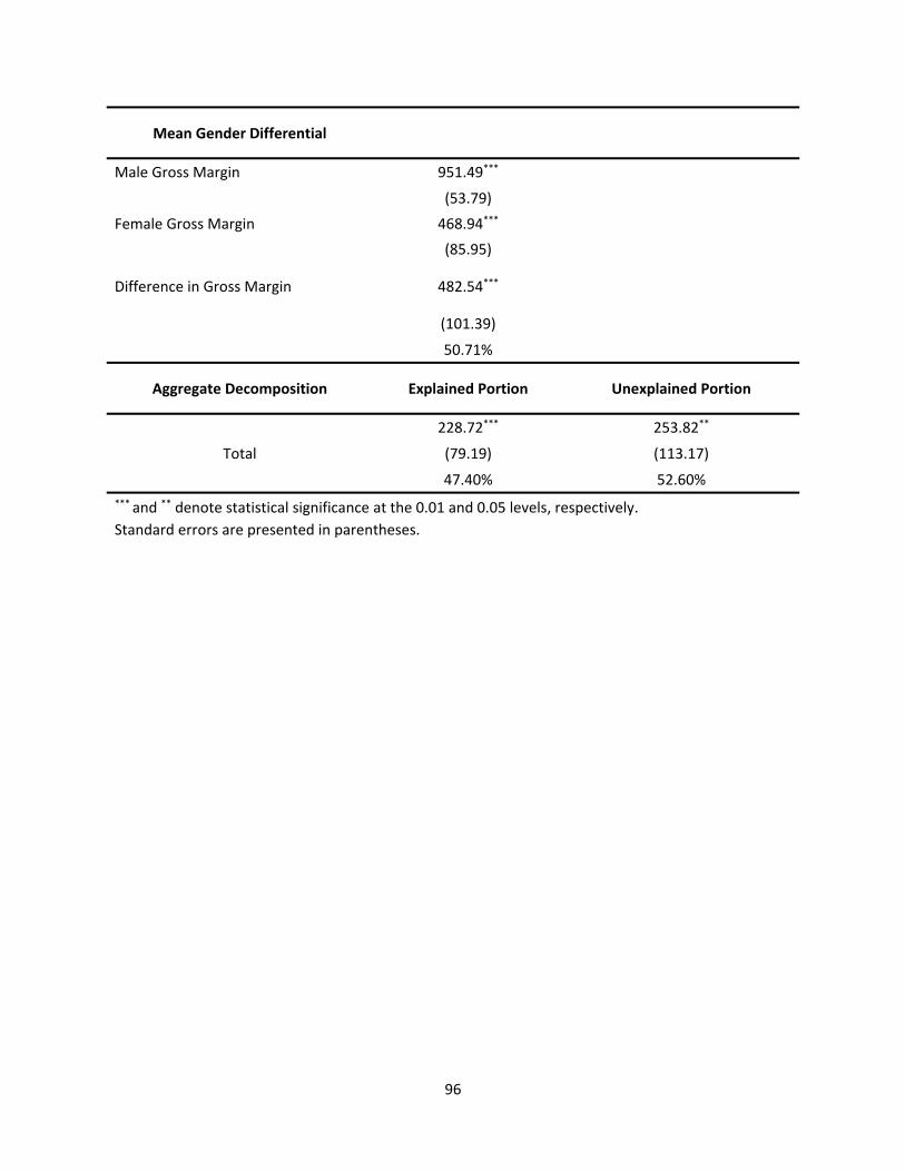
96
Mean Gender Differential
Male Gross Margin 951.49***
(53.79)
Female Gross Margin 468.94***
(85.95)
Difference in Gross Margin 482.54***
(101.39)
50.71%
Aggregate Decomposition Explained Portion Unexplained Portion
Total
228.72*** 253.82**
(79.19) (113.17)
47.40% 52.60%
*** and ** denote statistical significance at the 0.01 and 0.05 levels, respectively.
Standard errors are presented in parentheses.
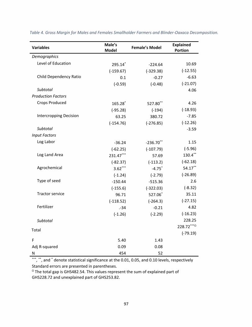
97
Table 4. Gross Margin for Males and Females Smallholder Farmers and Blinder‐Oaxaca Decomposition.
Variables Male’s Model
Female’s Model Explained Portion
Demographics
Level of Education 295.14* ‐224.64 10.69
(‐159.67) (‐329.38) (‐12.55)
Child Dependency Ratio 0.1 ‐0.27 ‐6.63
(‐0.59) (‐0.48) (‐21.07)
Subtotal 4.06
Production Factors
Crops Produced 165.28* 527.80** 4.26
(‐95.28) (‐194) (‐18.93)
Intercropping Decision 63.25 380.72 ‐7.85
(‐154.76) (‐276.85) (‐12.26)
Subtotal ‐3.59
Input Factors
Log Labor ‐36.24 ‐236.70** 1.15
(‐62.25) (‐107.79) (‐5.96)
Log Land Area 231.47*** 57.69 130.4**
(‐82.37) (‐113.2) (‐62.18)
Agrochemical 3.62*** ‐4.75* 54.17**
(‐1.24) (‐2.79) (‐26.89)
Type of seed ‐150.44 ‐515.36 2.6
(‐155.6) (‐322.03) (‐8.32)
Tractor service 96.71 527.06* 35.11
(‐118.52) (‐264.3) (‐27.15)
Fertilizer .‐34 ‐0.21 4.82
(‐1.26) (‐2.29) (‐16.23)
Subtotal 228.25
Total 228.72***Ω
(‐79.19)
F 5.40 1.43
Adj R‐squared 0.09 0.08
N 454 52 ***, **, and * denote statistical significance at the 0.01, 0.05, and 0.10 levels, respectively
Standard errors are presented in parentheses. Ω The total gap is GHS482.54. This values represent the sum of explained part of GHS228.72 and unexplained part of GHS253.82.
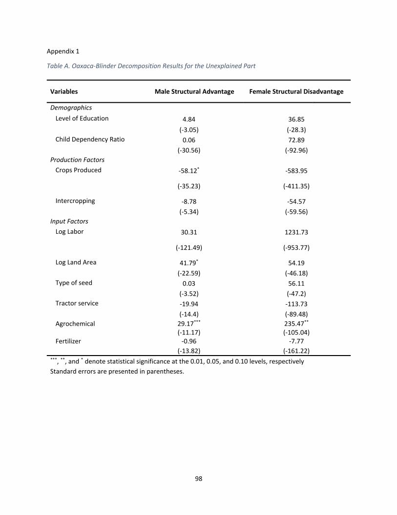
98
Appendix 1
Table A. Oaxaca‐Blinder Decomposition Results for the Unexplained Part
Variables Male Structural Advantage Female Structural Disadvantage
Demographics
Level of Education 4.84 36.85
(‐3.05) (‐28.3)
Child Dependency Ratio 0.06 72.89
(‐30.56) (‐92.96)
Production Factors
Crops Produced ‐58.12* ‐583.95
(‐35.23) (‐411.35)
Intercropping ‐8.78 ‐54.57
(‐5.34) (‐59.56)
Input Factors
Log Labor 30.31 1231.73
(‐121.49) (‐953.77)
Log Land Area 41.79* 54.19
(‐22.59) (‐46.18)
Type of seed 0.03 56.11
(‐3.52) (‐47.2)
Tractor service ‐19.94 ‐113.73
(‐14.4) (‐89.48)
Agrochemical 29.17*** 235.47** (‐11.17) (‐105.04)
Fertilizer ‐0.96 ‐7.77
(‐13.82) (‐161.22) ***, **, and * denote statistical significance at the 0.01, 0.05, and 0.10 levels, respectively
Standard errors are presented in parentheses.

99
Production Efficiency of Smallholder Farms in Northern Ghana25
Frank Nti, Yacob Zereyesus, Vincent Amanor‐Boadu, Kara Ross
Department of Agricultural Economics
Kansas State University
Abstract
The study uses household agricultural production survey data to estimate the level of production efficiency and factors that influence inefficiency for farm households in the three northern regions of Ghana. Results show managerial differences as the major factor impacting the overall technical efficiency scores. Returns to scale may not matter much for the analyzed farms since scale efficiency contribute less significantly to overall technical efficiency. Multi output production did not seem to improve production efficiency of the sampled farms. The use of policy instruments that support specialization in crops production and some educational or extension intervention will facilitate a reduction in yield gap, increase farm efficiency and improve the chronic food insecurity issues prevalent in the northern regions of Ghana.
Keywords: Efficiency, Data Envelopment Analysis (DEA), Northern Ghana, Food Security, Smallholder Farms
Introduction
Production efficiency of smallholder farms is of interest because of the immense contribution of
the productivity of smallholder farms to reducing food insecurity and improving livelihood in northern
Ghana. Knowing where a group of farms are with respect to the production efficiency frontier helps policy
makers develop and deliver effective intervention programs specific to the different groups of farms.
However, little is known about the production efficiencies of Ghanaian smallholder farmers producing
multiple crops, and the factors that constraint farm efficiencies. Only a few recent studies have
investigated efficiency of smallholder farm production for Ghana from a multi‐output multi‐input
perspective that accounts for the jointness in production (Abatania et al, 2012). But most subsistent
farmers produce multiple crops on either multiple plots or intercrop on a single plot and are likely to use
25 A previous version of this paper was presented at the International Food and Agribusiness Management
Association 25th Annual Congress, St. Paul, MN June 2015.

100
similar resources or inputs which are not divisible for each plot. Disaggregating the extent of resource use
on each plot for each crop could be particularly challenging, and if not appropriately done could influence
efficiency estimates for a single‐output multi‐input estimation framework.
As such, in this paper, we estimate the production efficiency for small holder farmers in northern
Ghana from a multi‐input multi‐output frame work and analyze farm characteristics and factors that
influence both efficiency and inefficiency alike. We focus on the production of three main crops – maize,
rice and soybean. These crops are important for northern Ghana farming households, because they form
the major food staples and have received considerable government and donor support to improve their
productivity. Yet, despite considerable investment in improving productivity through the introduction of
new varieties, and other technological changes, average yields under rained conditions are at best 1.7,
2.4 and 0.9 metric tons respectively (MOFA, 2010). However, under best agricultural practices, these crops
have demonstrated to grow at yields of 6, 4.5 and 4.5 metric tons respectively (MOFA, 2010). It is unclear
whether the yield gap differences between actual and attainable yields are due to production or scale
inefficiencies.
The objectives of the study are twofold. The first is to provide production efficiency estimates of
small holder farmers in northern Ghana that can be used to help data driven policy making. Efficiency
estimates for such farming households at the household level is rarely available. The second objective is
examine the impact of exogenous variables on small holder farm efficiency. We also sought the
application of recent developments in production efficiency analysis to improve the statistical efficiency
of estimates and account for data related problems for efficiency estimates. This was done by applying
Simar and Wilson’ s bootstrapping methods to the regressions estimates in the second stage regressions
discussed in subsequent sections.
For a sustained agricultural growth, a better understanding of the input use or mix and the impact
of managerial and socioeconomic factors on farm productivity are needed. These insights can lead to
improvements in farm productivity that is crucial to achieving the necessary improvements in food
production to reduce global hunger and malnutrition. Improving farm’s technical efficiency can increase
the ability to close the gap between current production and the efficient frontier given existing
technology, and improve the economic situation of farm households. Assuming technology is the same
across farms, low performing farms can improve production by imitating the production practices of the
more efficient farms without the need for new technology and additional resources. By estimating
technical (pure and overall) and scale efficiency for each farm unit, we attempt to implicitly evaluate the
impact of public programs on the economic performance of farming households in Northern Ghana.
101
The paper is structured as follows. The next section presents a review of methods for estimating
efficiencies. The method of analysis section introduces the Data Envelopment Analysis (DEA) estimation
procedure and the second stage regression. The data source and definition of variables are discussed in
the subsequent section. The results and discussion are presented next. Finally, a summary is presented.
Review of Methods
Researchers interested in farm production efficiency analysis typically use one of two approaches
to assess the ability to produce the maximum output possible from a given set of inputs or produce several
output quantities utilizing minimal inputs and production technology. The two approaches are a
stochastic parametric approach after Aigner et al. (1977) and a nonstochastic nonparametric approach
after Färe, Grosskopf, and Lovell (1985); Varian (1984); Chavas and Cox (1988); Chavas and Aliber (1993);
Featherstone, Langemeier, and Ismet (1997). Each of these approaches present its own unique
advantages and challenges which are duly documented in the literature (Bauer 1990; Coelli, 1995).
The parametric approaches, fit a functional form to observed data with an econometric method
to estimate the parameters. The production efficiency is based on the measured distance between the
observations and the estimated functional form (Featherstone, Langemeier, and Ismet, 1997). The
parametric approach captures the effects of exogenous shocks outside the control of the observed unit
by adding a symmetric error term to the model (Aigner et al., 1977; Meeusen and van den Broeck, 1977).
The hypothesis concerning the goodness of fit of the model used can also be tested under this approach.
Although the parametric approach accounts for the noise in the observed data by adding a symmetric
error term and also permit the estimation of standard errors for each efficiency score, it is not without
problems (Coelli, 1995). According to Varian (1984), the parametric form “must be taken on faith” since
the real functional form could never be tested. In addition, Bauer (1990) describes the parametric
approach as being weak since restrictions need to be imposed on the technology and this affects the
distribution of the efficiency terms.
In contrast, the nonparametric approach, as proposed by Färe, Grosskopf, and Lovell (1985), has
the desirable property of making fewer assumptions about the distribution and measurement of the
efficiency terms. This approach is independent of a functional form and impose no a prior assumptions
about the distributional structure underlying the data (Färe, Grosskopf, and Lovell, 1985; Chavas and
Aliber, 1993; Coelli, 1995; Featherstone, Langemeier, and Ismet, 1997; Bravo‐Ureta et al., 2007). A
weakness of this approach, however, is the inability to include statistical inference in the analysis and the
inability to account for any possible stochastic phenomena – measurement error or other noise in the
data – that can potentially bias the efficiency estimates (Hallam, 1992). As such, all deviations from the
102
frontier are attributed to inefficiency which may overstate technological inefficiencies. Another
disadvantage is its deterministic nature and effect on extreme observations (Bravo‐Ureta et al., 2007).
The potential sensitivity of the nonparametric efficiency scores to the number of observations, the
number of outputs and inputs, and the dimensionality of the frontier have also received much criticism in
the literature (Thiam, Bravo‐Ureta and Rivas, 2001; Ramanathan, 2003).
To address some of these concerns with the nonparametric deterministic approach, Simar and
Wilson (2007) developed the single or double bootstrap approach26. Its major contribution is the coherent
description of an underlying data‐generating process (DGP) with the simulation of a sampling distribution
for the nonparametric model. It provides consistent inference within data envelopment analysis (DEA)
model estimations and corrects the biased efficiency estimates that are produced from the traditional
DEA approach.
Methods of Analysis
First Stage DEA Estimation Procedure
Technical efficiency is defined under the DEA approach as the optimal input use for producing
several output quantities or the optimal output that could be produced with existing inputs or technology.
The DEA uses mathematical programming methods to measure technical efficiency. There are two ways
of implementing this approach: input orientation and output orientation. The input orientation estimates
the optimal input use for producing several output quantities and the output orientation estimates the
optimal output that could be produced with existing inputs or technology. The choice of either an output
orientation or an input orientation approach to estimate efficiency depends on the assumption on the
control the decision making units (DMU) have over their output or input variables respectively. In
agriculture, decision making units generally have little or no control over their output so the DEA approach
is input orientated. Using the input orientation for the first stage of the estimation process we assess the
proportional decrease in the input variables that can produce the same bundle of output under variable,
constant and non‐decreasing returns to scale technology assumptions for each farm unit. The efficiency
scores are bounded from above at one for perfectly efficient DMUs and bounded from below at zero for
26 Recent innovations in production efficiency analysis have indicated that bootstrapping techniques could improve the statistical efficiency of regression estimates as well as correct biases in the efficiency estimates. We explored Simar and Wilsons’ (2007) procedures to run the bootstrapping techniques. However, the bias-correcting single and double bootstrap procedures provided no improvements to the conventional DEA estimates in our first and second stage analyses.
103
perfectly inefficient DMUs. An efficiency score, , is calculated for the i‐th farm by solving the following
linear programming problem based on an input orientation procedure:
= max > 0| ≥ ∑ ; ≤ ∑ ; ≥ 0, = 1,… . , (1) where the number of farms is denoted by n, xi are the inputs, yi represents output levels, γi are
the non‐negative intensity weights, i represents the farm of interest, and is the measure of overall or
pure technical efficiency which differ by the assumption on the intensity scalar. To measure pure technical
efficiency ( ), the intensity scalar, γi,, in Equation 1is restricted to sum to one to allow the technology
function to allow for variable returns to scale. Pure technical efficiency reflects managerial capabilities in
organizing available resources. To measure overall technical efficiency ( ), constraint on the intensity
scalar is removed to allow for a constant returns to scale technology. A farm is technically efficient if =1, and technically inefficient if 0 < < 1. It is possible for a farm to exhibit pure technical efficiency
without overall technical efficiency due to the difference in its scale efficiency level. The measure of scale
efficiency ( ) is calculated by the ratio / and it defines the optimal or most productive scale of
operation. Farms producing in the region of decreasing returns to scale (DRS), increasing returns to scale
(IRS) or constant returns to scale (CRS) are evaluated using this condition: ≠ 1 and = reflects
increasing returns to scale and ≠ 1 and ≠ reflects decreasing returns to scale. is estimated by
imposing the constraint ∑ ≤ 1 on equation 1. Farms with increasing returns to scale (IRS) produce
in the decreasing region of the average cost curve with negative economic profit whiles farms with DRS
produce in the increasing region of the average cost curve with positive economic profit. Farms producing
at the minimum point of cost curve have zero economic profit and have CRS.
Second Stage Regression
Our second stage estimation procedure is organized as follows:
Step 1: Compute = ( , )∀ = 1,…… , by using Equation 1 under the assumption of
variable or constant returns to scale.
Step 2: Estimate = + using a truncated maximum likelihood estimation procedure,
where is the efficiency or inefficiency score from step one for each farm. is a vector of estimated
parameters for each input, , used and is the error term.
Two sets of analyses are conducted which follow the estimation procedure described above. In
the first analysis, the effect of institutional or policy variables (extension, commercialization, and
diversification) and a set of control variables (gender, education, location dummy and household size) are
examined on farm’s overall and pure technical inefficiency scores. The second set of analyses look at the
104
influence of non‐discretionary inputs – hired labor, family labor, communal labor, fertilizer cost, cost of
agrochemicals, land size and seed cost – on farm production efficiency scores (pure technical and overall).
The first assumes fixed discretionary inputs and assesses only the demographic variables’ effect on
efficiency. The second explicitly control for the discretionary inputs and evaluate their effect on efficiency.
Data
The data was collected in 2013/14 from 550 agricultural producing households in northern Ghana.
The data collection was funded by the United States Agency for International Development (USAID) under
the Monitoring, Evaluation and Technical Support Services (METSS) program in its effort to determine
performance in agricultural production. The study area covered 25 districts in four regions in Ghana –
Northern, Upper East, Upper West and Brong Ahafo (BA) regions. The data contains information on the
socioeconomic and managerial characteristics, the level of input use and output levels for 550 sampled
farms. A total of 113 observations including all observations for BA region were eliminated from the
analysis because of incomplete, inconsistent and missing data and to focus our analysis on only the three
northern regions. Total observations were therefore reduced to 437 farms. Data was also collected on five
input variables: labor, land, fertilizer, agrochemicals, and seed and the three output variables: maize, rice
and soybeans used in the non‐parametric DEA analysis.
The summary statistics of the input and output variables for our sampled farms are presented in
Table 1. We assumed our sampled farms located in the Upper East and West regions have similar
characteristics and were classified as “rural farms” whiles sampled farms in Northern region were
classified as “urban farms” for the purpose of our second stage estimation. Agricultural inputs used and
output produced varied across location. The average yields for urban farms were 0.82, 0.59, and 0.50
metric tons for maize, rice and soybeans respectively. The average yields for rural farms were 0.57, 0.30
and 0.21 metric tons for maize, rice and soybeans respectively. Even though these yields are far below
their national averages, some of the sampled farms recorded yields above the national averages (see
Table 1). The difference in the size of farm across location shows that urban farms are larger and with a
relatively more commercialization focus than rural farms. Yet, on average the rural smaller farms applied
more fertilizer to their farms than urban larger farms did. On average, rural farms (81 man‐days)
employed relatively higher labor inputs than urban farms (62 man‐days). However, the relative share of
average family labor turned out to be higher for urban farms (61%) than rural farms (51%).
Descriptive statistics of farm characteristics are summarized in Table 2. Most households are
headed by males (90%). The majority of farm managers have no formal education (88%). On average, a
household typically consist of ten people and are dependent on government‐supported institutions for

105
their seed supply. Many among the farms either intercropped or diversified their production (65%) but
farmed for subsistence purposes (64%). Extension service was not readily available to farmers and only
16% received technical assistance from extension agents.
Results and Discussion
DEA Production Efficiency Estimates
An assessment of Table 3 reveals that efficiency level varies across the different regions. Farms in
the Upper East region have efficiency advantage over farms in Northern and Upper West regions.
Approximately nine percent of all farms were found to be relatively overall technically efficient which
form the efficient frontier. These farms were used as the reference set of farms and produce utilizing the
relatively best available farm practice. Overall technical efficiency varied substantially from 0.013 to 1,
0.012 to 1 and 0.0158 to 1 for Northern, Upper West and Upper East regions respectively. The average
overall technical efficiency is higher for farms in Upper East Region (0.46) compared to farms in Northern
region (0.36) and Upper West Region (0.25). The mean overall technical efficiency for all farms across the
three regions was 0.38 and range from 0.012 to 1. This suggests that an average farm can potentially
increase current production by 2.6 times (1/0.38) when operating under a constant returns to scale
technology and utilizing the same level of inputs. Farms in Upper West have a relatively higher scope of
increasing output with the same level of inputs than farms in Upper East and Northern regions. More than
71% had an overall technical efficiency of below 50%. The level of overall technical efficiency is an
indication that most farms are either not operating under optimal scale or are not efficiently allocating
their factor inputs or both.
To analyze the pure technical efficiency, the restrictive weights on the level of factor inputs were
dropped to allow for a variable returns to scale technology. The mean efficiency across regions changed
less substantially from a constant returns to scale technology to a variable returns to scale technology.
The mean pure technical efficiency score for Northern, Upper East and Upper West regions were
estimated as 0.46, 0.57 and 0.36 respectively. Under variable returns to scale, pure technical efficiency
varied between 0.062 to 1, 0.058 to 1 and 0.11 to 1 for farms in Northern, Upper East and Upper West
regions respectively. The average overall PTE score (0.48) suggests that an average farm will need only
48% of current inputs to potentially produce the same output level if producing on the efficient frontier
under a variable returns to scale technology. These results also suggest that an average farm in Upper
East region allocates input more efficiently, followed by an average farm in Northern and Upper west

106
regions respectively. The distribution of farms according to efficiency scores reveals that not all farms that
were purely technically efficient or scale efficient were found to be overall technically efficient. Seventeen
percent had a pure technical efficiency of unity while only 15% were scale efficient.
The mean scale efficiencies were relatively higher than pure technical efficiencies at 76%, 79%
and 71% for farms in Northern, Upper East and Upper West regions respectively. Scale effect accounted
for only 20%, 15.6% and 14.6% of observed overall technical inefficiencies for farms in Upper East,
Northern and Upper West regions respectively. Thus, managerial differences are the major factors
impacting the overall technical efficiency rather than scale effect. There is a relatively higher potential to
increase farm productivity or bridge the yield gap through efficient input mix strategy in the short run
rather than a long run increment in farm size. The mean overall scale efficiency was 0.76 with a minimum
score of 0.049 and a maximum score of 1. This implies that the average scale inefficiencies for all farms
were about 24% and only about 16% of all inefficiencies for all farms were due to failure to operate on
optimal farm size. Nearly 60% of farms had a scale efficiency score of between 0.80 and 1.
Table 4 shows that only 15.6% of farms produced at the minimum point of the long run average
cost curve and thus fully exploit their scale economies. These farms operate at an optimal scale and
experience a constant returns to scale with zero economic profit. Seventy percent of farms operated in
the region of increasing returns to scale (decreasing average cost curve) and 14.4% operate in the region
of decreasing returns to scale (increasing average cost curve). Farms with increasing returns to scale (IRS)
operate below the most productive scale size with negative economic profit and farms in the decreasing
returns to scale (DRS) region produce above their optimal scale size with positive economic profit. With
increasing returns to scale predominating all forms of scale inefficiency, farmers are expected to increase
their scale of production to take advantage of the positive scale effect.
Sources of Inefficiency
After establishing the potential level of efficiency for each farm relative to the most efficient set
of farms in the sample, it is important to understand the sources of the inefficiencies in production (overall
and pure technical inefficiencies). The results reveals that household size and diversification exhibited
positive and statistically significant influences on inefficiency under both technology specifications. This
implies that larger households tend to be associated with inefficient resource allocation. This may be
explained by the increase in family labor without equivalent increase in other resources, leading to a lower
marginal labor productivity. Another implication of this results could be that, the production of any of the
commodities is independent of the decisions about the other commodities (i.e. non‐jointness in input
usage may exist).

107
One would expect scope economies gain through diversification or intercropping to lower
inefficiencies but the coefficient on diversification is in contrast to a prior expectation. This suggest that
the jointness in production does not provide any significant economic gains from the use of factor inputs.
Perhaps other factors not explicitly accounted strongly influence farmers decision to intercrop or diversify
their production. Other possible source of inefficiency include extension service. Under the VRS
specification, an access to technical assistance correspond to increasing pure technical inefficiency. This
result raises a number of empirical questions surrounding the effectiveness, appropriateness and
timeliness of extension services available to farmers in the study area. Farmers may not be provided the
necessary or right information, or extension agent are less equipped with the requisite training and tools
to be efficient information agents and or information provided to farmers are based off generally
acceptable practices and not on research findings peculiar to their ecological area.
Sources of Input Efficiency
Now we turn our attention to factors that influence the level of technical efficiency. Estimation
for the conventional truncated model reveals land and labor as statistically significant for both CRS and
VRS specification. In addition, communal labor and seed cost are statistically significant for the VRS
specification. A larger land size enables farmers to take advantage of potential scale economies to improve
production efficiency. As shown in Table 6 communal labor and family labor are sources of inefficiency for
sampled farms. This supports findings pertaining to the coefficient of household size. In our estimation
process we assumed all members in the family as part of the total family labor. No information on the
number of family members that directly partake in farm activities were available and thus the number of
family labor may have been overstated. The results suggest that increasing family and communal labor
beyond their optimal levels will significantly decrease farm efficiency. There exist surplus labor in the
agricultural sector of the study area which could be absorbed or transferred to other existing productivity
sectors. Expansion of the opportunities for the surplus labor to engage in non‐farm employment should
be a primary policy target.
A lower seed cost improves farm efficiency, indicating that smallholder farms perform better
when seeds are affordable. Most of the farmers in our sample depended on government supported
institutions for their seed supply, hence the removal of government‐supported subsidies on seeds have
the potential to negatively impact smallholder farmers’ ability to produce maximum output level.
Conclusion

108
This article presented an analysis of production efficiency and the source of inefficiency among
farms in the three regions in the northern part of Ghana from a multi‐input multi‐output framework. The
efficiency estimations for a multi‐input multi‐output production framework was necessitated by the
presence of possible jointness in the production system – the sampled farms produce multiple products
with an allocable fixed input such as land in their production function.
We first estimated technical efficiency (CRS), pure technical efficiency (VRS) and scale efficiency
and the inefficiencies were calculated by subtracting each efficiency score from one. The efficiency level
changed less significantly from a CRS to VRS and across the three regions. The estimated results suggest
that the major source of overall technical inefficiency were from farms managerial inefficiency rather than
failure to operate on optimal land size. The mean pure technical efficiency was 0.48, suggesting the
potential to produce the same output level with only 48% of current inputs if farms utilizes best
production practices. Alternatively, with the given input level an average farm can potentially produce 2.6
times as much output under a constant returns to scale technology. From a policy perspective, closing
yield gap in production will require a more focus on improving farms pure technical efficiency or input mix
(managerial efficiency) rather than farms operating with optimal scale of resource.
The econometrics results suggest that a larger household size and crop diversification contributes
to farms lower technical efficiencies. Farms with access to extension do not have a relative advantage
compared to those without access in terms of efficiency improvement. This phenomenon raises empirical
questions surrounding local extension services in the study area. From the estimates of the relative
importance of factors on productivity, land area expansion and reduction in family labor were found to
be significant contributors to farm productivity. Farmers could take advantage of the scale effect by
increasing their land size in the long run.
Returns to scale may not be that relevant for the analyzed farms (scale efficiency contribute less
significantly to overall technical efficiency). Rather managerial differences was shown as the major factor
impacting the overall technical efficiency scores. Multi output production did not seem to improve
production efficiency of sampled farms. The use of policy instruments that support specialization in crops
production and some educational or extension intervention will facilitate the reduction in the yield gap,
increase farm efficiency and improve the chronic food insecurity issues prevalent in the northern regions
of Ghana.
References

109
Abatania, L. N., Hailu, A. & Mugera, A. W. (2012) Analysis of farm household technical efficiency in
Northern Ghana using bootstrap DEA. Conference (56th), February 7‐10, 2012, Freemantle,
Australia, 2012. Australian Agricultural and Resource Economics Society.
Aigner, D.J., C.A.K. Love11 and P. Schmidt, (1977). Formulation and estimation of stochastic frontier
production function models, Journal of Econometrics 6, 21‐37.
Bauer, P.W. (1990). “Recent developments in the econometric estimation of frontiers.” Journal of
Econometrics. 46:39‐56.
Bravo‐Ureta, B. E., D. Solis, V.H. Moreira Lopez, J. F. Maripani, A. Thiam, and T. Rivas. (2007). “Technical
efficiency in farming: a meta‐regression analysis.” Journal of Productivity Analysis. 27:57‐72.
Chavas, J. P., and M. Aliber. (1993). “An Analysis of Economic Efficiency in Agriculture: A Nonparametric
Approach.” Journal of Agricultural and Resource Economics. 18: 1‐16.
Chavas, J. P., and T. L. Cox. (1988). “A Nonparametric Analysis of Agricultural Technology.” American
Journal of Agricultural Economics. .70: 303‐310.
Coelli, (1995). “Estimators and Hypothesis Tests for a Stochastic Frontier Function: A Monte Carlo
Analysis”, Journal of Productivity Analysis, 6, 247‐268.
Fare, R., S. Grosskopf and C.A.K Lovell. (1985). The measurement of efficiency of production. Boston:
Kluwer‐Nijhoff.
Featherstone, A. M., M. R. Langemeier, and M. Ismet. (1997). “A Nonparametric Analysis of Efficiency for
a Sample of Kansas Beef Cow Farms.” Journal of Agricultural and Applied Economics. 29:175‐184.
Hallam, A. (1992) “A Brief Overview of Nonparametric Methods in Economics.” Northeastern Journal of
Agricultural and Resource Economics. 21:98‐112.
Ministry of Food and Agriculture, (2010). Statistics, Research and Information Directorate
http://mofa.gov.gh/site/wp‐content/uploads/2011/04/mofa_facts_and_figures.pdf
Meeusen, W. and van den Broeck, J. (1977). Efficiency Estimation from Cobb‐Douglas production
functions with composed error. International Economic Review, 18: 435–444.
Ramanathan, R. (2003). An introduction to data envelopment analysis: a tool for performance
management. SAGE Publications: Thousand Oaks, CA.
Simar, L., & Wilson, P. W. (2007). Estimation and inference in two‐stage, semi‐parametric models of
production processes. Journal of econometrics, 136(1), 31‐6
Thiam, A., B. E. Bravo‐Ureta, T. E. Rivas. (2001). “Technical efficiency in developing country agriculture: a
meta‐analysis.” Agricultural Economics 25: 235‐243.
Varian, H.R. (1984). “The Nonparametric Approach to Production Analysis.” Econometrica, 52: 579‐597.

110
Appendix
Table 1: Summary Statistics for the sample farms according to region
Units
All region Urban Farm Households
Rural farm Households
Mean SD Mean SD Mean SD DEA Model Maize Kg 735.65 672.29 820.46 726.67 574.65 520.07 Rice Kg 438.53 449.05 587.14 534.15 296.89 288.77 Soybeans Kg 437.36 318.75 501.35 309.18 206.31 240.87 Land Ha 1.27 1.63 1.47 1.35 0.92 1.99 Fertilizer Kg 105.04 123.02 91.13 114.56 129.35 133.49 Labor Man-
days 69.42 63.71 62.56 50.40 81.43 80.75
Agrochemical Kg 5.78 27.47 8.33 33.65 1.32 8.13 Maize Seed Kg 37.88 104.17 45.25 120.98 24.52 61.39 Rice Seed Kg 70.93 205.64 116.94 286.39 27.18 35.39 Soybean Seed Kg 31.77 30.14 35.73 30.29 15.69 24.19 Second-stage regression (with Efficiency) Seed Cost $US 11.33 30.61 12.21 35.42 9.78 19.55 Fertilizer Cost $US 111.47 138.06 95.28 128.65 139.79 149.39 Agrochemical cost
$US 20.88 34.61 29.52 38.89 5.79 17.11
Family labor Man-days
39.41 44.48 38.28 40.49 41.37 50.79
Hired labor Man-days
17.91 36.58 12.77 21.57 26.89 52.42
Communal labor Man-days
12.10 24.59 11.50 20.04 13.15 31.04
Second-stage regression (with Inefficiency) Diversification Binary 0.64 0.47 0.65 0.47 0.64 0.48 Commercialization
Binary 0.36 0.48 0.42 0.49 0.25 0.43
Extension Binary 0.16 0.36 0.13 0.34 0.20 0.40 Region Binary 0.36 0.48 0 0 1 0 Gender Binary 0.89 0.30 0.93 0.24 0.83 0.37 Household size Person
s 10.65 5.82 10.99 6.02 10.05 5.42
Educate Binary 0.12 0.32 0.097 0.29 0.15 0.36
Table 2: Explanatory variables in the second‐stage regression (with inefficiency)
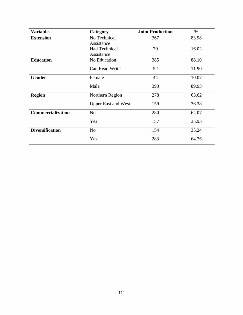
111
Variables Category Joint Production % Extension No Technical
Assistance 367 83.98
Had Technical Assistance
70 16.02
Education No Education 385 88.10
Can Read Write 52 11.90
Gender Female 44 10.07
Male 393 89.93
Region Northern Region 278 63.62
Upper East and West 159 36.38
Commercialization No 280 64.07
Yes 157 35.93
Diversification No 154 35.24
Yes 283 64.76

112
Table 3: Summary Statistics of Efficiency Measures
OTE PTE SE Northern Region Mean 0.36 0.46 0.76
SD 0.29 0.31 0.27 Min 0.013 0.062 0.049 Max 1 1 1
Upper East Mean 0.46 0.57 0.79 SD 0.32 0.31 0.27 Min 0.012 0.058 0.079 Max 1 1 1
Upper West Mean 0.25 0.36 0.71 SD 0.19 0.22 0.29 Min 0.0158 0.11 0.085 Max 1 1 1
All Regions Mean 0.38 0.48 0.76 SD 0.29 0.31 0.27 Min 0.012 0.058 0.049 Max 1 1 1
Distribution of Farms
Less than 0.10 71 9 5 0.10 to < 0.20 95 85 18 0.20 to < 0.30 66 75 22 0.30 to < 0.40 42 59 22 0.40 to < 0.50 44 50 19 0.50 to < 0.60 24 24 24 0.60 to < 0.70 17 17 31 0.70 to < 0.80 19 22 37 0.80 to < 0.90 14 10 56 0.90 to < 1.00 7 11 138
1 38 75 65

113
Table 4: Returns to Scale of the small holder farms in Northern Ghana
Returns to Scale Multiproduct % CRS 68 15.6 DRS 63 14.4 IRS 306 70.0
Table 5: Conventional technical inefficiency regression estimates
Coefficient Standard Error
Confidence Interval
CRS Household size 0.0056** 0.001931 0.001851 0.009421 Region -0.0278 0.037855 -0.08578 0.062607 Gender -0.0115 0.024619 -0.07607 0.020441 Educate 0.0037 0.036132 -0.06709 0.074545 Extension 0.0318 0.031597 -0.03009 0.093767 Commercialization -0.0157 0.02675 -0.06812 0.036733 Diversification 0.1411*** 0.026357 0.089459 0.192778 VRS Household size 0.0060** 0.002028 0.00212 0.010069 Region 0.0171 0.037509 -0.05638 0.090651 Gender -0.0422 0.024356 -0.08999 0.005487 Educate -0.0075 0.035955 -0.07799 0.062946 Extension 0.0899** 0.031316 0.028602 0.151358 Commercialization -0.0102 0.026695 -0.06254 0.042103 Diversification 0.1084*** 0.026229 0.057014 0.159831
Note: *,**, *** denote 10%, 5% and 1% level of significance Number of observations = 438
Table 6: Conventional technical efficiency regression estimates
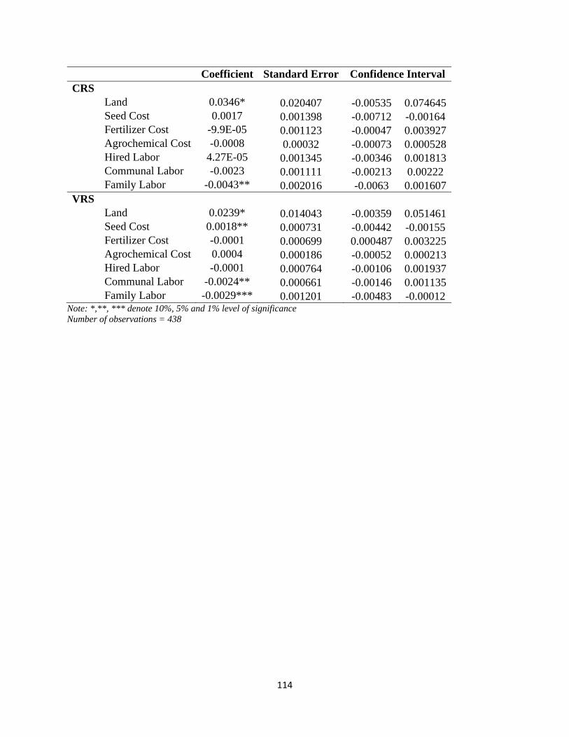
114
Coefficient Standard Error Confidence Interval CRS Land 0.0346* 0.020407 -0.00535 0.074645 Seed Cost 0.0017 0.001398 -0.00712 -0.00164 Fertilizer Cost -9.9E-05 0.001123 -0.00047 0.003927 Agrochemical Cost -0.0008 0.00032 -0.00073 0.000528 Hired Labor 4.27E-05 0.001345 -0.00346 0.001813 Communal Labor -0.0023 0.001111 -0.00213 0.00222 Family Labor -0.0043** 0.002016 -0.0063 0.001607 VRS Land 0.0239* 0.014043 -0.00359 0.051461 Seed Cost 0.0018** 0.000731 -0.00442 -0.00155 Fertilizer Cost -0.0001 0.000699 0.000487 0.003225 Agrochemical Cost 0.0004 0.000186 -0.00052 0.000213 Hired Labor -0.0001 0.000764 -0.00106 0.001937 Communal Labor -0.0024** 0.000661 -0.00146 0.001135 Family Labor -0.0029*** 0.001201 -0.00483 -0.00012
Note: *,**, *** denote 10%, 5% and 1% level of significance Number of observations = 438

115
Does Women’s Empowerment in Agriculture Matter in Children’s Health
Status? Insights from Northern Ghana
Yacob A. Zereyesus, Vincent Amanor‐Boadu and Kara Ross
Department of Agricultural Economics Kansas State University, Manhattan, KS 66506
September 2014
Abstract
The association between women’s empowerment in agriculture and children’s latent health
status is examined for a sample of households in northern Ghana using a Multiple Indicators Multiple
Causes (MIMIC) model. The MIMIC approach is used to link multiple indicator variables with multiple
independent variables through a “single underlying” latent variable. Height‐for‐age and weight‐for‐
height are used as indicators of the underlying children’s health status and women’s empowerment in
agriculture and control variables are used as the multiple independent variables. Our results show that
neither the composite empowerment score used to capture women’s empowerment in agriculture nor
its decomposed components are statistically significant in their association with the latent children’s
health status. However, the associations between children’s health status and control variables such as
child’s age, mother’s education, household’s hunger scale and residence locale are statistically
significant. Of the two health status indicators,‐height‐for‐age scores and weight‐for‐ height scores,‐the
former exhibited a stronger association with the latent health status. While promoting women’s
empowerment to enhance their ability to make strategic life choices, it is important to carefully consider
how the achievement of these objectives will impact the women’s wellbeing and the well‐being of the
children in their care.
Key words: Women’s empowerment in agriculture; latent variable; Height‐for‐age; weight‐for‐height; MIMIC

116
Introduction
Healthy children perform well in school and achieve higher educational attainment because they
are more likely to be attentive (Brown and Pollitt 1996; Rivera et al. 1995). Educational attainment has
been shown to correlate with incomes (Psacharopoulos and Patrinos 2004) as well as mental and
physical state (Duflo 2000). Thus, children’s health status is deemed an important factor in their
ultimate human capital capacity and economic productivity (Alderman et al. 2006; Behrman 1996;
Grantham‐McGregor et al. 1999; Victora et al. 2008).
Women, as the traditional caregivers of children (especially in rural communities in developing
countries) (Saaka et al. 2009) are particularly responsible for the nutrition and other health‐related
decisions affecting children in their care. The choices available to women caregivers are not
independent of their own capabilities, resources and freedoms to make independent decisions (Boateng
et al. 2014). Interest in women’s ability to make independent choices, framed as women’s
empowerment, has become an increasingly important subject in economic development circles over the
past few decades (Doan and Bisharat 1990; Narayan 2002; Alsop et al. 2006). Although women’s
empowerment is a complex and multidimensional concept, the general consensus is that women’s
empowerment refers to “the enhancement of women’s ability to make strategic life choices.” (Malhotra
and Schuler 2005 pp. 84). Women’s empowerment can contribute to achieving development goals such
as poverty reduction and gains in human capital formation such as improved health status for women
and education. These positive externalities can also lead to increases in agricultural productivity,
income growth, and improvements in child health (Smith et al. 2003).
Given women’s role as primary caregivers of children, it is plausible to assume that their
empowerment would influence the health status of their children. Previous studies have assessed the
association of various forms of women’s empowerment on a single measure of children’s health status
(Desai and Johnson 2005; Heaton and Forste 2008). This paper aims to explore the empirical association
between women’s empowerment in agriculture and the health status of children in their care. The
current study takes advantage of a recently developed aggregate index used to measure women’s
empowerment in broader rural settings, whether they are farmers, agricultural or non‐agricultural wage
workers, or engaged in non‐farm businesses (Alkire et al. 2013). Although the index can be adapted to
measure empowerment to any rural occupation, the focus of the current study is on those women who
are engaged in the agriculture sector. The paper assesses the association of the composite and
decomposed components of the Women’s Empowerment in Agriculture Index (WEAI) (Alkire et al. 2013)
on a latent children’s health status represented by two indicators: height‐for‐age; and weight‐for‐

117
height. The rest of the paper is organized as follows: the data and methods section presents the nature
and sources of the data and the development of the model. This is followed by the main empirical
results and discussions of the study. Conclusions and policy implications are summed up in the last
section.
Data and Methods
Data
Ghana is a West African country, with an estimated population in 2012 of about 24 million.
Although it has been performing very well against the Millennium Development Goals of the United
Nations (United Nations 2000), Ghana’s performance is uneven across its administrative regions (Osei‐
Assibey and Grey 2013). For example, the three northernmost regions were all found to be lagging
behind the national average on poverty reduction goals. As a result of this uneven progress, the
majority of development agencies, including the U.S. Agency for International Development (USAID), are
now focusing their development efforts in the northern part of the country.
We use data from the 2012 population‐based survey conducted in the area above Ghana’s
Latitude 8°N of , covering the administrative regions of Brong Ahafo, Northern, Upper East and Upper
West but excluding the areas falling in Volta Region. The total population in the study area was
estimated at about 5.2 million in 2012, a little over 20 percent of the country’s total population.
The survey was commissioned by USAID with an objective of providing baseline estimates for
about a dozen Feed the Future initiative indicators it needed to track for the monitoring and evaluation
of its intervention activities in the study area. There were 4,410 households and nearly 25,000 men,
women and children included in the survey. However, only 1,393 of women aged less than 50 years
(reproductive age women) are included in this research because they were the ones who had children
below five years of age in their care. Probability weights are used to facilitate study area population
representativeness of the estimates. In addition to demographic and socio‐economic information, the
survey collected data on children and women’s anthropometry, and data to facilitate the estimation of
the Women’s Empowerment in Agriculture Index (WEAI), household hunger scale and women’s dietary
diversity scale.
The current research was approved for compliance with federal, state or local rules, regulations
and guidelines by the appropriate Research Compliance Office, the Committee on Research Involving
Human Subjects which serves as the Institutional Review Board (IRB).

118
Endogenous Variables
The observable endogenous variables that represent the underlying children’s health status are
the anthropometric indicators of height‐for‐age and weight‐for‐height. These two observable
anthropometric indicators represent the unobservable children’s health status outcome variable. It is
noted that well‐nourished children 10 years or younger, regardless of country and ethnic backgrounds,
have similar height and weight distribution and growth rates (Cogill 2003). This allows for the
development of a reference population which may be used to facilitate anthropometric comparisons. It
is therefore necessary to standardize the anthropometric indicators for using them in any analysis
(United Nations 2006a). The standardization involves developing the z‐score, ijZ , for each child, j, in the
sample and each anthropometric indicator, i, such that:
( )ij ij Mi MiZ V V (1)
where ijV is the observed value for the ith indicator of the jth child, and MiV and Mi are the
median and the standard deviation of the ith indicator in the reference population. When ijZ for any
child is more than 2 standard deviations below VMi,, then that child is stunted or wasted for i equals
height‐for‐age or weight‐for‐height, respectively.
Exogenous Variables
Two models are explored in this study; the difference between them is that one uses the
composite score used to capture Women’s Empowerment in Agriculture Index (WEAI) and the other
uses the principal components of the WEAI as explanatory variables. Both models also use demographic
and socio‐economic characteristics of the children and their parents as exogenous variables as well as
household hunger and the diversity in participating women’s diets.
WEAI has two weighted sub‐indexes: the Five Domains of Empowerment (5DE); and the Gender
Parity Index (GPI) (Alkire et al. 2013). The 5DE and the GPI indexes have 90 percent and 10 percent of
the weights in the derivation of the WEAI. The GPI measures a woman’s empowerment relative to her
male household counterpart. The 5DE, on the other hand, assesses a woman’s empowerment in
decision‐making and control across five domains examined under the WEAI: production, resources,
income, leadership, and time. The production domain assesses a woman’s sole or joint decision‐making
authority in agricultural production, whether crop or livestock farming or fisheries. The resources
domain assesses ownership, access to, and decision‐making power over productive resources such as
land, livestock, agricultural equipment, credit, and consumer durables while the income domain

119
assesses whether sole or joint control over income and expenditures. The leadership domain explores a
woman’s membership in economic or social groups and her comfort speaking in public while the time
domain evaluates her satisfaction with the distribution of her time between work and leisure. Each of
the 5DE comprises one, two or three components, giving rise to a total of ten components, each of them
allocated a weight the sum of which is unity (Figure 1). The weighted sum of stated inadequacies in the
ten components for each woman provides the inadequacy count (CI). A woman is considered
disempowered if her CI is at least 20 percent (Alkire et al. 2013). Recall that we explore the effect of
both the composite and decomposed forms of the WEAI. In its composite form, we treat the CI as a
continuous variable. However, in the decomposed form, we treated each component as a dummy
variable.
Figure 1: Adequacy criteria for the ten indicators in the five domains of empowerment
Indicator Adequacy Criteria Weight
Production
Input in Productive Decisions
A woman is adequate if she participates or feels she has input in at least two types of decisions.
1/10
Autonomy in Production
A woman has adequate achievement if her actions are motivated more by her values as opposed to her fear of disproval or feelings of coercion.
1/10
Resources
Ownership of assets
A woman is adequate if she has joint or sole ownership of at least one major asset.
1/15
Purchase, sale, or transfer of assets
On assets owned by a household, a woman is adequate if she is involved in the decisions to buy, sell, or transfer assets.
1/15
Access to and decisions on credit
An adequate woman belongs to a household that has access to credit and when decisions on credit are made, she has input in at least one decision regarding at least one source credit.
1/15
Income Control over use of income
A woman is adequate if she has some input (or perceived input) on income decisions provided that she participated in the income generating activity.
1/5
Leadership
Group Member A woman is considered adequate if she is a member of at least one group from a wide range of economic and social groups.
1/10
Speaking in Public
A woman is deemed adequate if she is comfortable speaking in public in at least one context.
1/10
Time
Leisure Time A woman has adequate leisure time if she does not express any level of dissatisfaction with the amount of leisure time available.
1/10
Work Burden A woman is considered to have an excessive workload and thus, inadequate if she worked more than 10.5 hours in the previous 24 hours.
1/10
Source: Alkire et. Al 2013.
The remaining exogenous variables are the same in both models. They include women’s dietary
diversity score, household hunger scale and the socio‐economic characteristics of mother’s age, both
father and mother’s education, household income, residence locale, child’s gender and age. Due the
high risk of safe water on health, we also include access to portable drinking water as a dummy

120
exogenous variable. It may be expected that the exogenous variables will exhibit multicollinearity.
However, the Variance Inflation Factor (VIF) values for all the variables were below 2, suggesting that
these variables were not collinear.
The Women’s Dietary Diversity Score (WDDS) is developed using a count of nine food groups
consumed over 24 hours preceding the interview (Kennedy et al. 2011). There are three categories of
the score: (i) Low – consuming foods from no more than three food groups; (ii) Medium – consuming
foods from four to five food groups; and (iii) High – consuming foods from more than five of the food
groups. The Household Hunger Scale (HHS) is a simple indicator for tracking household hunger in food
insecure areas (Ballard at al. 2011). The HHS is estimated from answers to a series of questions about
food accessibility and the frequency of food insecurity over a 4‐week or 30‐day recall period (Ballard at
al. 2011). The food insecurity of a household is considered severe when the HHS is between 4 and 6 and
moderate when it between 2 and 3. The household is considered to have little or no hunger when its
HHS is between 0 and 1. Table 1 presents the definition and summary statistics of the variables used in
the models.
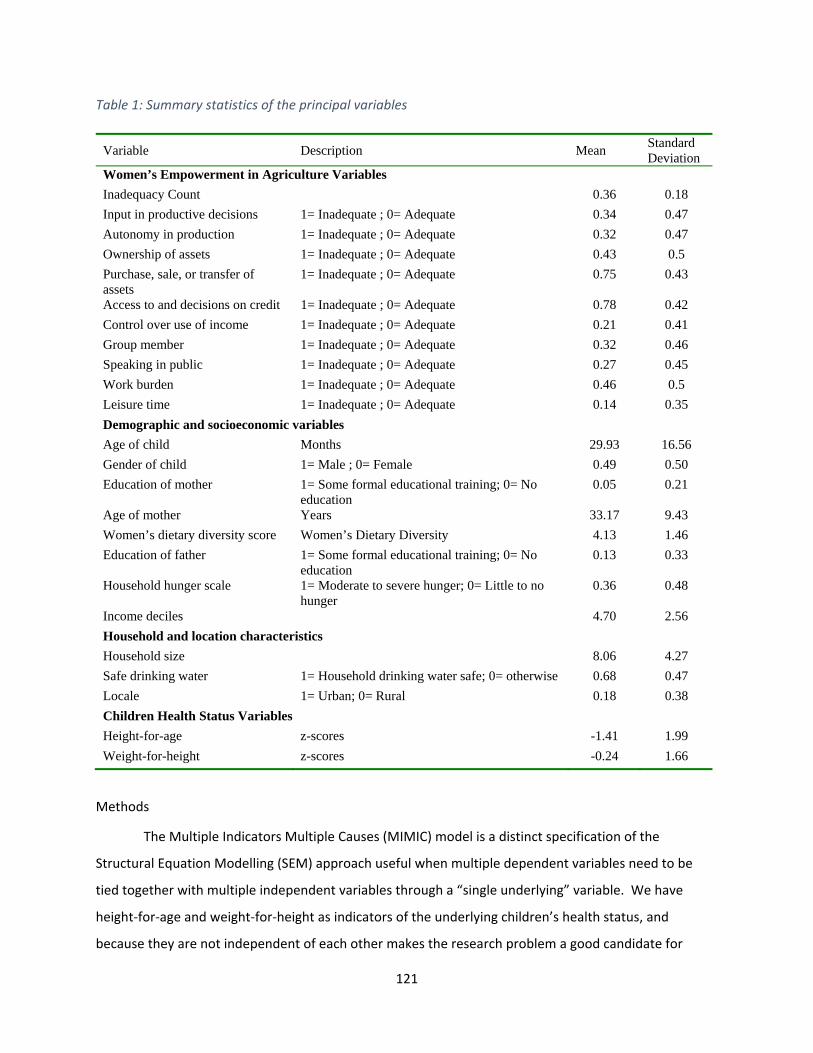
121
Table 1: Summary statistics of the principal variables
Variable Description Mean Standard Deviation
Women’s Empowerment in Agriculture Variables
Inadequacy Count 0.36 0.18
Input in productive decisions 1= Inadequate ; 0= Adequate 0.34 0.47
Autonomy in production 1= Inadequate ; 0= Adequate 0.32 0.47
Ownership of assets 1= Inadequate ; 0= Adequate 0.43 0.5
Purchase, sale, or transfer of assets
1= Inadequate ; 0= Adequate 0.75 0.43
Access to and decisions on credit 1= Inadequate ; 0= Adequate 0.78 0.42
Control over use of income 1= Inadequate ; 0= Adequate 0.21 0.41
Group member 1= Inadequate ; 0= Adequate 0.32 0.46
Speaking in public 1= Inadequate ; 0= Adequate 0.27 0.45
Work burden 1= Inadequate ; 0= Adequate 0.46 0.5
Leisure time 1= Inadequate ; 0= Adequate 0.14 0.35
Demographic and socioeconomic variables
Age of child Months 29.93 16.56
Gender of child 1= Male ; 0= Female 0.49 0.50
Education of mother 1= Some formal educational training; 0= No education
0.05 0.21
Age of mother Years 33.17 9.43
Women’s dietary diversity score Women’s Dietary Diversity 4.13 1.46
Education of father 1= Some formal educational training; 0= No education
0.13 0.33
Household hunger scale 1= Moderate to severe hunger; 0= Little to no hunger
0.36 0.48
Income deciles 4.70 2.56
Household and location characteristics
Household size 8.06 4.27
Safe drinking water 1= Household drinking water safe; 0= otherwise 0.68 0.47
Locale 1= Urban; 0= Rural 0.18 0.38
Children Health Status Variables
Height-for-age z-scores -1.41 1.99
Weight-for-height z-scores -0.24 1.66
Methods
The Multiple Indicators Multiple Causes (MIMIC) model is a distinct specification of the
Structural Equation Modelling (SEM) approach useful when multiple dependent variables need to be
tied together with multiple independent variables through a “single underlying” variable. We have
height‐for‐age and weight‐for‐height as indicators of the underlying children’s health status, and
because they are not independent of each other makes the research problem a good candidate for
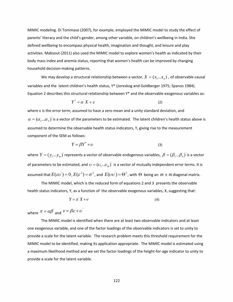
122
MIMIC modeling. Di Tommaso (2007), for example, employed the MIMIC model to study the effect of
parents’ literacy and the child’s gender, among other variable, on children’s wellbeing in India. She
defined wellbeing to encompass physical health, imagination and thought, and leisure and play
activities. Mabsout (2011) also used the MIMIC model to explore women’s health as indicated by their
body mass index and anemia status, reporting that women’s health can be improved by changing
household decision‐making patterns.
We may develop a structural relationship between a vector, '1 )...( nxxX , of observable causal
variables and the latent children’s health status, Y* (Joreskog and Goldberger 1975; Spanos 1984).
Equation 2 describes this structural relationship between Y* and the observable exogenous variables as:
* 'Y X (2)
where ε is the error term, assumed to have a zero mean and a unity standard deviation, and
'1 )...( n is a vector of the parameters to be estimated. The latent children’s health status above is
assumed to determine the observable health status indicators, Y, giving rise to the measurement
component of the SEM as follows:
*Y Y (3)
where '1 )...( myyY represents a vector of observable endogenous variables, '
1( ... )n is a vector
of parameters to be estimated, and '1 )...( m is a vector of mutually independent error terms. It is
assumed that 0)( ' E ,22 )( E , and
2' )( E , with being an m x m diagonal matrix.
The MIMIC model, which is the reduced form of equations 2 and 3 presents the observable
health status indicators, Y, as a function of the observable exogenous variables, X, suggesting that:
XY ' (4)
where ' and
' v
The MIMIC model is identified when there are at least two observable indicators and at least
one exogenous variable, and one of the factor loadings of the observable indicators is set to unity to
provide a scale for the latent variable. The research problem meets this threshold requirement for the
MIMIC model to be identified, making its application appropriate. The MIMIC model is estimated using
a maximum likelihood method and we set the factor loadings of the height‐for‐age indicator to unity to
provide a scale for the latent variable.

123
The exogenous variables in our model have different units, making any comparison of their
estimated parameters uninformative. Bollen (1989) provides solution to this problem, suggesting
standardization of the estimated parameters to eliminate their units, and in doing so, make them
comparable. This is akin to economists using elasticities to determine the relative importance of the
contributions of variables. The problem with the elasticity metaphor is that the contribution approaches
infinity as the point of the estimation approaches zero. Bollen’s (1989) solution avoids this problem by
standardizing using standard deviations. From Equation 2 and Equation 3 above, the standardized
parameter estimates, sij and s
ij , are therefore defined as:
ii
jjij
sij
ˆ
ˆˆˆ and
ii
jjij
sij
ˆ
ˆˆˆ
where i is the dependent variable, j is the explanatory variable, ii and jj are the model‐predicted
standard deviations of the ith and jth variables, respectively. The standardized parameter estimates show
the change in standard deviation units of the dependent variable resulting from a one standard
deviation change in an explanatory variable, ceteris paribus.
Results
Table 2 shows the results of the two models: the composite WEAI using respondents’
inadequacy count as a continuous variable; and the decomposed WEAI using the 5DE components as
binary variables. When probability weights are applied to make the estimated results representative of
the entire population, goodness of fit indicators are given by the Standardized Root Mean Squared
Residuals (SRMR).The SRMR scores for both specifications were less than 0.05, indicating good fit of the
models. The association between the composite inadequacy count (CI) index used to capture women’s
empowerment in agriculture and children’s health status is not statistically significant in northern
Ghana, where the study occurred. Similarly, the associations between the decomposed WEAI
components and children’s health status are not statistically significant. Previous studies using different
formats of the composite women’s empowerment index have produced mixed results. Desai and
Johnson (2005), for example, found no statistically significant association between women’s autonomy
and children’s height‐for‐age in Benin, Uganda, Zimbabwe, Egypt, Nepal, Colombia, Nicaragua and Peru.
However, they reported significant positive association in India and Mali, and significant negative
association in Malawi. Heaton and Forste (2008) also found no association between women’s autonomy

124
and children’s height‐for‐age in Colombia, Peru, Nicaragua and Bolivia, but a negative association in
Haiti.
Table 2: Results of the structural MIMIC model
Specification 1 Specification 2
Standardized Coefficient
Standard Error
Standardized Coefficient
Standard Error
Input in productive decisions 0.030 0.036
Autonomy in production 0.042 0.040
Ownership of assets 0.075 0.040
Purchase, sale, or transfer of ‐0.050 0.040
Access to and decisions on 0.016 0.045
Control over use of income ‐0.038 0.041
Group member ‐0.019 0.035
Speaking in public 0.053 0.038
Work burden ‐0.060 0.033
Leisure time ‐0.001 0.026
Inadequacy count 0.005 0.032
Child's age ‐0.217*** 0.050 ‐0.231*** 0.053
Child's gender ‐0.037 0.035 ‐0.046 0.039
Mother's education 0.062** 0.030 0.074** 0.033
Mother's age 0.057 0.033 0.063 0.035
Women’s dietary diversity score
0.050 0.032 0.054 0.031
Father's education ‐0.001 0.030 ‐0.002 0.032
Household hunger scale 0.105*** 0.033 0.101*** 0.034
Income deciles 0.006 0.043 0.011 0.049
Household size 0.110 0.058 0.105 0.065
Safe drinking water 0.056 0.035 0.055 0.040
Locale 0.098** 0.040 0.107** 0.042
**, *** denote significance of standardized coefficients at the 95 % and 99 % confidence levels, respectively. The Standardized Root Mean Squared Residual (SRMR) for both specifications are 0.009 and the R-squared for specification 1 and 2 are 0.10 and 0.12, respectively.
To the best of our knowledge, no research has been conducted on assessing the association
between the individual components of the 5DE and children’s health status. What our results show is
that none of the 10 components exhibited a statistically significant association with children’s health
status in the study area. However some of the control variables are associated with children’s health
status. In both specifications, child’s age and household’s hunger scale have a statistically significant
association with children’s health status at the 1 percent level while mother’s education and locale,

125
defined as whether the family lived in a rural or urban area are determined to have a statistically
significant association with children’s health status at the 5 percent level. The signs on both parameter
estimates are as expected, i.e., the higher a child’s age, the lower the associated height‐for‐age score,
and the more educated the child’s mother, the higher the child’s height‐for‐age score. This result is in
agreement with previous results that suggest mother’s education is positively correlated with the
children’s well‐being in Uganda (Shariff and Ahn1995). Children living in urban areas are also associated
with having higher height‐to‐age scores. The associations between children’s health status and family
income, father’s education, and drinking water are not statistically significant. The results also provide
additional information on the estimated standardized coefficients. For example, the marginal analysis of
the standardized coefficients show that, holding other factors constant, a one standard deviation shift in
child’s age would shift child’s health status by 0.22 and 0.23 standard deviations in Model Specification 1
and 2 respectively.
The results from the measurement models also reveal the magnitude and strength of the
association between the health status variable and its constituent indicators (Tables 3).The statistically
significant coefficients of the height‐for‐age and weight‐for‐height scores confirm the existence of the
underlying ‘single’ common latent variable. Furthermore, the factor loadings indicate that the
underlying common health status variable is more associated with the height‐for‐age than with the
weight‐for‐height scores. Thus, a one standard deviation change in the latent health status variable is
associated with 0.94 standard deviation change in the height‐for‐age score and about 0.36 standard
deviation change in the weight‐for‐height score. The different signs on the estimated coefficients of the
two indicators of children’s health status reveal the negative correlation between them.
Table 3: Results of the measurement MIMIC model
Specification 1 Specification 2
Standardized Coefficient
Standard Error
Standardized Coefficient
Standard Error
Height‐for‐age 0.990*** 0.164 0.940*** 0.185
Weight‐for‐height ‐0.336*** 0.071 ‐0.359*** 0.090 *** denotes significance of standardized coefficients at the 99% confidence level. The R-squared values for specifications 1 and 2 are 0.98 and 0.88, respectively. Implications and Conclusions
Women’s empowerment has become an increasingly important factor in economic
development. There has, therefore, been an increasing interest to identify the importance of its role in
influencing development indicators, such as children’s health status. The motivation for this research
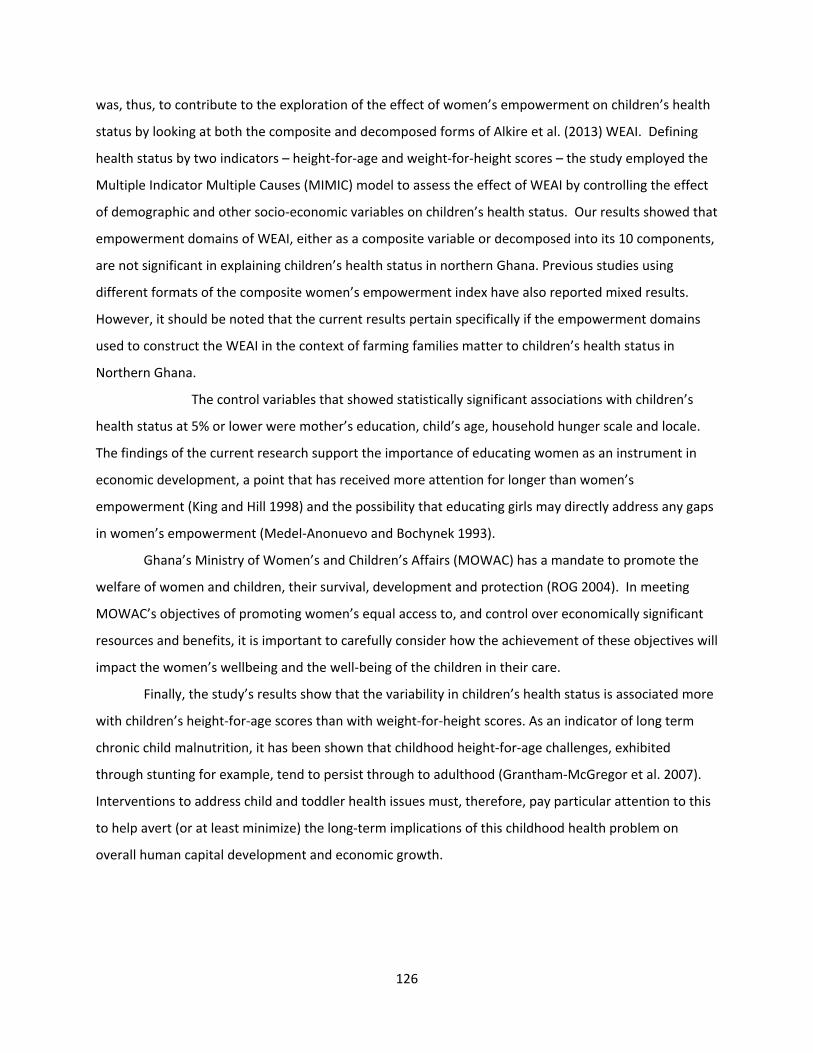
126
was, thus, to contribute to the exploration of the effect of women’s empowerment on children’s health
status by looking at both the composite and decomposed forms of Alkire et al. (2013) WEAI. Defining
health status by two indicators – height‐for‐age and weight‐for‐height scores – the study employed the
Multiple Indicator Multiple Causes (MIMIC) model to assess the effect of WEAI by controlling the effect
of demographic and other socio‐economic variables on children’s health status. Our results showed that
empowerment domains of WEAI, either as a composite variable or decomposed into its 10 components,
are not significant in explaining children’s health status in northern Ghana. Previous studies using
different formats of the composite women’s empowerment index have also reported mixed results.
However, it should be noted that the current results pertain specifically if the empowerment domains
used to construct the WEAI in the context of farming families matter to children’s health status in
Northern Ghana.
The control variables that showed statistically significant associations with children’s
health status at 5% or lower were mother’s education, child’s age, household hunger scale and locale.
The findings of the current research support the importance of educating women as an instrument in
economic development, a point that has received more attention for longer than women’s
empowerment (King and Hill 1998) and the possibility that educating girls may directly address any gaps
in women’s empowerment (Medel‐Anonuevo and Bochynek 1993).
Ghana’s Ministry of Women’s and Children’s Affairs (MOWAC) has a mandate to promote the
welfare of women and children, their survival, development and protection (ROG 2004). In meeting
MOWAC’s objectives of promoting women’s equal access to, and control over economically significant
resources and benefits, it is important to carefully consider how the achievement of these objectives will
impact the women’s wellbeing and the well‐being of the children in their care.
Finally, the study’s results show that the variability in children’s health status is associated more
with children’s height‐for‐age scores than with weight‐for‐height scores. As an indicator of long term
chronic child malnutrition, it has been shown that childhood height‐for‐age challenges, exhibited
through stunting for example, tend to persist through to adulthood (Grantham‐McGregor et al. 2007).
Interventions to address child and toddler health issues must, therefore, pay particular attention to this
to help avert (or at least minimize) the long‐term implications of this childhood health problem on
overall human capital development and economic growth.

127
References
Alderman, H., Hoddinott, J., and Kinsey, B. (2006). Long term consequences of early childhood
Malnutrition. Oxford Economic Papers 58, 450–74.
Alkire, S., Meinzen‐Dick, R., Peterman, A., Quisumbing, A., Seymour, G., and Vas, A. (2013). The women’s
empowerment in agriculture index. World Development, 52, 71–91
Alsop, R., M. Bertelsen, and J. Holland. (2006). Empowerment in practice from analysis to
implementation. Washington, DC: World Bank.
Ballard, T., J. Coates, A. Swindale, and M. Deitchler. 2011. “Household Hunger Scale: Indicator Definition
and Measurement Guide.” Washington, DC: Food and Nutrition Technical Assistance (FANTA) II
Project, FHI 360.
Behrman, J. (1996). The impact of health and nutrition on education. World Bank Research Observer 11,
23–37.
Boateng, G.O., V.Z. Kuuire, M. Ung, J.A. Amoyaw, F.A. Armah, and I. Luginaah. (2014). Women’s
empowerment in the context of Millennium Development Goal 3: A case study of married
women in Ghana. Social Indicators Research 115, 137‐158.
Bollen, K. A. (1989). Structural equations with latent variables. New York: John Wiley & Sons.
Brown J.L, and E. Pollitt. (1996). Malnutrition, poverty and intellectual development. Scientific American
274: 38‐43.
Cogill, B. (2003). Anthropometric indicators measurement guide. Washington, DC: Food and Nutrition
Technical Assistance (FANTA) Project, FHI 360.
Desai, S. and K. Johnson. (2005). Women’s decision‐making and child health: Familial and social
hierarchies. In S. Kishor, (ed.) A focus on gender – collected papers on gender using DHS data
ORC Macro: Calverto, 15–33.
Di Tommaso, M. L. (2007). Children capabilities: A structural equation model for India. The Journal of
Socio‐Economics, 36(3), 436–450.
Doan, R., and L. Bisharat. (1990). Female autonomy and child nutritional status: The extended‐family
residential unit in Amman, Jordan. Soc Sci Med, 31, 783–789.
Duflo, E. (2000). Child health and household resources in South Africa: Evidence from the old age
pension program. The American Economic Review, 90(2), 393‐398.
Grantham‐McGregor, S., Cheung, Y. B., Cueto, S., Glewwe, P., Richter, L., Strupp, B., et al. (2007).
Developmental potential in the first 5 years for children in developing countries. Lancet,
369(9555), 60‐70.

128
Grantham‐McGregor, S., L.Fernald, and K. Sethuraman. (1999). Effects of health and nutrition on
cognitive and behavioural development in children in the first three years of life: part 1: Low
birthweight, breastfeeding and protein‐energy malnutrition. Food and Nutrition Bulletin, 20, 53‐
75.
Heaton, T.B. and R. Forste. (2008). Domestic violence, couple interaction and children’s health in Latin
America. Journal of Family Violence, 23,183‐193.
Joreskog, K.G. and A.S. Goldberger. (1975). Estimation of a model with multiple indicators and multiple
causes of a single latent variable. Journal of the American Statistical Association ,70(351), 631‐
639.
Kennedy, G., T. Ballard, and M. Dop. (2011). Guidelines for measuring household and individual dietary
diversity. United Nations, Food and Agriculture Organization: Nutrition and Consumer
Protection Division.
King, E.M. and M.A. Hill. (1998).Women’s education in developing countries barriers, benefits, and
policies. Baltimore: Published for the World Bank, the Johns Hopkins University Press.
Mabsout, R. (2011). Capability and health functioning in Ethiopian households. Social Indicators
Research, 101,359‐389.
Malhotra, A., and Schuler, S. R. (2005). Women’s Empowerment as a variable in international
development. In D. Narayan (Ed.), Measuring Empowerment: Cross‐Disciplinary Perspectives
(pp. 71‐88). Washington, DC: World Bank
Medel‐Anonuevo, C. and B. Bochynek. (1993). International seminar on women’s education and
empowerment. In C. Medel‐Anonuevo (Ed.) Women, Education and Empowerment: Pathways
towards Autonomy. Hamburg, Germany: UNESCO Institute for Education.
Narayan, D. (2002). Empowerment and poverty reduction. Washington, DC: World Bank.
Osei‐Assibey, E. and S.K. Grey. (2013). Millennium Development Goals in Ghana. 2010 Population and
Housing Census Report, Ghana Statistical Service.24.
Ballard, T., J. Coates, A. Swindale, and M. Deitchler. (2011). Household Hunger Scale: IndicatorDefinition
and Measurement Guide. Washington, DC: Food and Nutrition Technical Assistance (FANTA) II
Project, FHI 360.
Psacharopoulos, G., and H.A. Patrinos. (2004). Returns to investment in education: A further update.
Education Economics, 12,111‐134.
129
Rivera, J.A., R.Martorell, M.T. Ruel, J.P. Habicht, and J.D. Haas. (1995) .Nutritional supplementation
during the preschool years influences body size and composition of Guatemalan adolescents
Journal of Nutrition, 125 (suppl), 1068S–77S.
ROG (Republic of Ghana). (2004). National gender and children policy. Retrieved October 14, 2014, from
http://www.hsph.harvard.edu/population/womenrights/ghana.gender.04.pdf
Saaka, M., J. Oosthuizen, and S. Beatty. (2009). Effect of prenatal zinc supplementation on birthweight.
Journal of Health Population and Nutrition, 27,619‐631.
Shariff, A., N. Ahn. (1995). Mother’s education effect on child health: An econometric analysis of child
anthropometry in Uganda. Indian Economic Review, 30 (2), 203‐222.
Smith, L. C., U. Ramakrishnan, A. Ndiaye, L. Haddad, and R. Martorell. 2003. The importance of women’s
status for child nutrition in developing countries. Research Report 131, International Food Policy
Research Institute.
Spanos, A. (1984). Liquidity as a latent variable: An application of the MIMIC model. Oxford Bulletin of
Economics and Statistics, 46(2), 125‐143
United Nations .2000. Resolution Adopted by the General Assembly. Retrieved on October 14, 2014
from http://www.un.org/millennium/declaration/ares552e.pdf
United Nations, World Health Organization. (2006a). Multicentre Growth Reference Study Group. WHO
Child Growth Standards: length/height‐for‐age, weight‐ for‐age, weight‐for‐length, weight‐for‐
height and body mass index‐for‐age: Methods and development. Geneva.
Victora, C.G. L. Adair, C. Fall, P.C. Hallal, R. Martorell, L. Richter, and H.S. Sachdev. (2008). Maternal and
child undernutrition: Consequences for adult health and human capital. Lancet, 371: 340‐357.

130
Recent Evidence of Health Effects of Women Empowerment: A Case
Study of Northern Ghana27
Kara Ross, Yacob Zereyesus, Aleksan Shanoyan, and Vincent Amanor‐Boadu
Department of Agricultural Economics
Kansas State University
Abstract
Women empowerment could be the key to unlocking women’s productivity potential in Africa. Women’s contribution to the agricultural sector is greatly influenced by their health status. This paper examines the impact of women’s empowerment in agriculture on women’s health and the implications for the African food and agricultural sector. It utilizes a unique dataset from a 2012 survey of 2,405 women in northern Ghana and the Multiple Indicators Multiple Causes modeling approach. Findings provide insight on how gender‐sensitive policies and private‐public initiatives can translate into better health outcomes for women and improved capacity to meet future needs of food and agriculture in Africa. Initiatives focusing on increasing women’s membership in social and economic groups, easing women’s access to credit, and increasing women’s incomes are some key empowerment strategies for improving women’s health status and production capabilities.
Key words: women empowerment, agriculture, health, Ghana, Africa
Introduction
Women play a significant role in the agricultural sector in developing countries. Recent
evidence from developing countries indicates that women supply, on average, 43 percent of the
agricultural labor force, but in Sub‐Saharan Africa, this contribution is nearly 50 percent (FAO 2011).
They also constitute a significant proportion of the wage workers in the agri‐food supply chain (FAO
2011, 2010). In addition to their roles in agriculture, women have a vital role in household production
and are usually the primary care givers within the household.
A woman’s role, responsibilities, and activities in household production and, particularly, in
agricultural production are time consuming and physically demanding, requiring significant energy and
physical capacity. This implies that women’s ability to effectively undertake these agricultural and
household production activities is greatly influenced by their physical capability and their health status.
27 A previous version of this paper was published in the International Food and Agribusiness Management
Review, Feb 2015.

131
Smith et al. (2003) states that improving women’s health status can effectively enhance their
performance in their socioeconomic responsibilities, including increasing agricultural production by
becoming more efficient and skilled laborers.
A woman’s health status is influenced by her access to and control over resources that affect
food availability and her ability to be responsible for her health care needs (Mabsout 2011, Sahn and
Younger 2009). Therefore, the empowerment of women to have more decision rights over the
dimensions of their lives that affect their health and capability in performing income generating and
care giver responsibilities has been receiving significant attention in recent years (De Schutter 2013, FAO
2011).
Empowering women is a complex concept given the socio‐cultural dimensions embedded in
gender relations and politics (Samman and Santos 2009). This complexity also confounds the
development of a good definition for the concept of women’s empowerment. The two main elements
that are widely accepted in the definition of empowerment are “process” and “agency”. Empowerment
is considered to be a process, a transition in an individual’s decision‐making capability from where she is
denied choices to a position where she has the ability to choose for herself. The second element,
agency, states that an individual must play a role in this process of change. The concept of agency is the
“ability to define one’s goals and act upon them” (Kabeer 1999). These two key elements are expressed
in the following definition for women’s empowerment that is adopted in the study: “women’s ability to
make decisions and affect important outcomes for themselves and their families as well as have control
over their life and over their resources” (Malhotra, Schuler, and Boender 2002).
The purpose of this study is to gain insights into the relationship between women’s
empowerment in agriculture and women’s health status. This research uses survey data that includes a
newly developed index, Women Empowerment in Agriculture Index (WEAI). The WEAI is designed to
meet the need for a robust and comparable tool that measures the empowerment, agency, and
inclusion of women in the agricultural sector. This study contributes to the literature by utilizing the
WEAI to examine the impact of women’s empowerment in agriculture on women’s health status. To the
authors’ best knowledge, this is the first peer‐reviewed research study to analyze these survey data and
the WEAI in relation to women’s health status in northern Ghana. The Multiple Indicators Multiple
Causes (MIMIC) model is used to assess how two primary indicators of women’s physical health status ‐
body mass index (BMI) and women’s dietary diversity score (DDS) ‐ are influenced by empowerment and
autonomy indicators. The paper hypothesizes that a greater degree of women’s empowerment and

132
decision‐making capabilities leads to a higher health status. The insights gained from testing this
hypothesis will contribute to a greater understanding of how women’s empowerment in agriculture is
associated with women’s health status. The findings from this study can help guide public‐private
initiatives in developing more appropriate and effective empowerment strategies that are focused on
improving the health and well‐being of women in northern Ghana. These strategies may also help to
enhance women’s productivity in agriculture in northern Ghana and other Sub‐Saharan Africa countries.
Health is a complex multidimensional concept, encompassing physical, mental and emotional
components of an individual. For the purpose of this study, only the physical aspect of health will be
examined. Universally accepted physical health measures that are commonly used are BMI and
women’s DDS. BMI is an unobtrusive measure and is defined as the ratio of an individual’s weight in
kilograms to her height in meters squared (kg/m2) (WHO 2014, CDC 2014). BMI provides a reliable
measure for body composition, which is used in health screenings for potential health problems
associated with body weight. BMI is both age and gender independent, making this measurement very
versatile, consistent, and easy to compute. The women’s DDS serves as an indicator of women’s
consumption of diverse foods with adequate micronutrients and nutritional quality, which is universally
recognized as a key component of healthy diets. This score helps identify if particular micronutrient
deficiencies exist within a certain population, and it also provides insights for policy makers and health
professionals to effectively promote good health and diets with adequate intake of essential nutrients.
Each of these health measures is assumed to be a component of a woman’s health status, which is
unobserved.
Methods
In this study, a special specification of the Structural Equation Modeling (SEM) approach is used,
the Multiple Indicators Multiple Causes (MIMIC) model. This MIMIC model is an ideal model to use
when multiple dependent variables need to be associated with a “single” variable. Two women’s health
status indicators represent the dependent variables in this research – BMI and DDS. Since these
indicators are not independent of each other, the MIMIC model is more appropriate for this analysis
than other traditional structural equation models. The MIMIC model was used by Mabsout (2011) to
study women’s health as indicated by their BMI and anemia status. The results from his study indicated
that women’s health can be improved by changing household decision‐making patterns.
Following Joreskog and Goldberger (1975) and Spanos (1984), a vector, '
1( ... )nK k k, of
observable latent causes of a woman’s health status, *H is developed. Equation 1 describes this

133
relationship with the error term, ε, assumed to have a zero mean and a unity standard deviation, and
'1( ... )na a a
is a vector of the parameters to be estimated:
* 'H a K (1)
It is assumed that the latent women’s health status determines the observable health status
indicators of interest in this study, H. This relationship is expressed in Equation 2 as follows:
*H bH (2)
where '
1( ... )mH h hrepresents a vector of observable endogenous variables,
'1( ... )nb b b
is a
vector of parameters to be estimated, and '
1 )...( m is a vector of mutually independent error
terms. It is assumed that 0)( ' E ,22)( E , and
2' )( E , with being an m x mdiagonal
matrix.
The MIMIC model, which is the reduced form of equations (1) and (2), presents the observable
health status indicators, H, as a function of the observable exogenous variables, K, suggesting that:
'
( )
H K
where ab and b
(3)
At least two observable indicators and at least one exogenous variables are needed to ensure
that the MIMIC model is identified, provided that one of the factor loadings of the indicators is set equal
to one to form the scale of the latent variable. Since the problem in this study meets the criteria for
identification, the MIMIC model can be used in the estimation. The MIMIC model is estimated by the
maximum likelihood method.
The exogenous variables do not all have the same units, which makes comparison among the
variables uninformative. Following the approach recommended by Bollen (1989), the coefficients are
standardized to eliminate their measurements. Standardization of the coefficients will allow
comparisons across the variables. It is essentially the same approach as elasticities, which are
commonly used by economists to determine the relative importance of the contributions of variables in
134
a model and provides the same information. We can determine which independent variables’ one
percent change leads to the largest percent change in dependent variables. With elasticities, the
contribution or effect of the independent variable approaches infinity as the point of estimation reaches
zero. The point of estimation is typically the mean. Thus, a mean of zero results in no solution.
To avoid this risk, other unitless indicators are used to determine relative influence. The
standardized regression coefficients, ˆ s
ija and
ˆsijbare represented as follows:
ˆˆ ˆ
ˆjjs
ij ij
ii
a a
and
ˆˆ ˆ
ˆjjs
ij ij
ii
b b
where i is the dependent variable, j is the explanatory variable, ii and ˆ
jj are the model‐predicted
standard deviations of the ith and jth variables, respectively. The standardized coefficients represent
the mean response in standard deviation units of the dependent variable for a one standard deviation
change in the explanatory variables, ceteris paribus.
The outcome of interest is women’s health status measured by the BMI and DDS indicators.
These indicators, therefore, are the dependent variables in the estimation models. The explanatory
variables are the WEAI and the ten principal components of the WEAI, as well as the demographic and
socio‐economic characteristics of the women. The summary statistics, along with the variable
definitions, are presented in Table 1.
Data
The research uses data from a USAID‐funded, population‐based survey conducted during July
and August of 2012 in northern Ghana. A two‐stage stratified random sampling technique is adopted in
the survey, and probability weights are developed to account for differential probabilities of selection
and non‐responses from the households, resulting in a design representative of the population in
northern Ghana. For this particular study, the focus is on the health conditions of the self‐identified
primary woman in each household. Primary members of the household are the ones responsible for
making social and economic decisions, and are, typically, a husband and wife.
The study sample is comprised of 4,513 women, aged 15 to 49 years, with complete dietary
diversity information and anthropometric measurements. There are 23 women with “extremely high”
BMI measurements for their weight/height profiles; they are treated like outliers and excluded from the

135
study’s sample. Of the remaining 4,490 women, 2,405 are the primary women and are the focus of this
study.
Health Indicators: BMI and DDS
BMI is currently considered the standard in determining nutritional status and health risk
conditions (Wells and Fewtrell 2006). It provides a very economical way to classify people by their
potential health riskiness: BMI of less than 18.5 kg/m2 are underweight; BMI between 18.50 kg/m2 and
24.99 kg/m2 is normal; and BMI greater than 25 kg/m2 is overweight or obese. Women with BMI values
in the underweight category face a serious problem in developing countries, given their role in the
economic well‐being and health of their families. For women whose daily economic activities involve
agricultural and other physically‐demanding work, being underweight impedes their ability to perform
their activities efficiently. Women who are underweight spend more time performing their daily
activities (Kennedy and Garcia 1994), and they are at a higher risk of developing functional disabilities
(Ferraro et al. 2002) compared to their counterparts with BMIs in the normal range. Kennedy and
Garcia (1994) show that having a healthy (or normal) BMI increases the capacity to perform domestic
and agricultural activities.
The women’s DDS is estimated using a count of nine food groups consumed over the preceding
24 hours; the food groups were developed by Kennedy et al. (2011). The nine food groups are: (1)
starchy staples; (2) dark green leafy vegetables; (3) other vitamin A rich fruits and vegetables; (4) other
fruits and vegetables; (5) organ meat; (6) meat and fish; (7) eggs; (8) legumes and nuts; and (9) milk and
milk products. The three categories of the DDS score – low, medium, and high – are based on the
number of these food groups consumed (Kennedy et al. 2011). A low DDS has no more than three of
the food groups, while a medium DDS includes four to five of the food groups. A high DDS represents
the consumption of more than five of the food groups. Dietary diversity scores have been positively
correlated with macronutrient and micronutrient adequacy of diets for adults (Olge et al. 2001, Foote et
al. 2004, Arimond et al. 2010). Savy et al. (2005) report a positive relationship between dietary diversity
scores and nutritional status of adult women in rural Burkina Faso. Bhagowalia et al. (2012) found that
Bangladeshi women who have a greater level of empowerment, as measured by their education, height,
and attitudes towards abuse, decision‐making power, and mobility, were associated with greater dietary
diversity scores and reduced levels of stunted children. Low DDS may present risks of micronutrient
deficiencies, such as iron deficient anemia, that can affect a woman’s ability to provide adequate care
for her family and lower her income‐generating potential (Haddad et al. 1994, WHO 2013).
Table 1: Summary Statistics

136
Women’s Empowerment in Agriculture Index (WEAI)
The WEAI is a newly developed survey‐based index that was created to monitor and evaluate
women’s empowerment in the agricultural sector. Development of the WEAI was a collaborative effort
between USAID, International Food Policy Research Institute (IFPRI), and the Oxford Poverty and Human
Development Initiative (OPHI). The WEAI measures the multi‐dimensional aspects of gender inequality
in agriculture. Previous empowerment measures are limited in their ability to measure women’s
decision‐making and autonomy outside of the household and domestic activities (Alkire et al. 2012).
Given the importance of women in agriculture, it is essential to have a tool, such as WEAI, that measures
the effect of agriculture interventions on women’s empowerment within that sector. The WEAI is
constructed using two weighted sub‐indices developed by Alkire et al. (2012): (1) The Five Domain
Variable Description Mean Std. Dev
Demographic and Socio‐economic Variables
Age Years 32.32 7.93
Education 1 = Some formal educational training; 0 = No education 0.09 0.28
Marital Status 1 = Married/Cohabitation; 0 = Not Married/ Cohabitating 0.96 0.20
Income Deciles 5.14 2.76
Household Hunger Scale 1= Moderate to severe hunger; 0 = Little to no hunger 0.38 0.48
Household Characteristics and Location Variables
Household Size Household members 6.21 3.08
Safe Drinking Water 1 = Household drinking water is safe; 0 = is not safe 0.70 0.46
Access to Electricity 1 = Access to electricity; 0 = No access to electricity 0.27 0.45
Private Toilet 1 = A private toilet in household; 0 = No toilet 0.14 0.35
Urban Locale 1 = Urban; 0 = Rural 0.23 0.42
Women Empowerment in Agricultural Variables
WEAI Inadequacy Count Inadequate > 0.20 0.34 0.18
Input in Productive Decisions 1 = Inadequate; 0 = Adequate 0.33 0.47
Autonomy in Production 1 = Inadequate; 0 = Adequate 0.26 0.44
Ownership of Assets 1 = Inadequate; 0 = Adequate 0.44 0.50
Purchase, Sale, or Transfer of Assets 1 = Inadequate; 0 = Adequate 0.73 0.44
Access to and Decisions on Credit 1 = Inadequate; 0 = Adequate 0.79 0.41
Control over Use of Income 1 = Inadequate; 0 = Adequate 0.22 0.42
Group Member 1 = Inadequate; 0 = Adequate 0.29 0.45
Speaking in Public 1 = Inadequate; 0 = Adequate 0.30 0.46
Leisure Time 1 = Inadequate; 0 = Adequate 0.13 0.34
Work Burden 1 = Inadequate; 0 = Adequate 0.45 0.50
Women Well‐being Variables
BMI Underweight if BMI < 18.5 22.33 3.62
DDS Score ranges from 0 to 9 3.99 1.59
Total Sample 2,405

137
Empowerment Index (5DE); and (2) The Gender Parity Index (GPI).28 The 5DE index encompasses five
domains of empowerment: production, resources, income, leadership, and time. The GPI, on the other
hand, measures the empowerment of women compared to their male counterparts in the household.
Thus, GPI is useful for male and female gendered households and not particularly useful when employed
for female only gendered households. Given the study’s focus on women’s health and their
empowerment, the GPI dimension is not included in the analyses.
The 5DE is constructed from the weighted summation of the adequacy scores of the ten
indicators in the index’s five domains. A woman is empowered if she is deemed adequate in four out of
the five domains or has a score that reflects at least 80 percent adequacy (Alkire et al. 2012). In this
study’s sample, the average inadequacy score is 0.34, which is above the inadequacy threshold of 0.20
set by Alkire et al. (2012). Of the 2,405 respondents interviewed about women’s empowerment, 1,740
have inadequacy scores above the threshold. In other words, over 72 percent of the women in this
study are considered to not yet be empowered. Compared to other African countries where the WEAI
survey has been conducted, Ghana has the highest rate of women who are not yet empowered;
followed by Liberia and Kenya at 70 percent, and Zambia with 60 percent. At 30 percent, Rwanda has
the lowest rate, and Uganda and Malawi have the second and third lowest rates, 42 and 48 percent,
respectively (Malapit et al. 2014).
Table 2 provides the criteria used to determine adequacy in the ten indicators. For example, the
production domain consists of two indicators that evaluate a woman’s role in joint and sole decision‐
making with regards to agricultural practices and autonomy in agricultural product decisions, such as
input purchases, livestock and cropping decisions, and whether or not to participate in marketing
activities. In the survey, the autonomy questions focus on whether a woman makes a decision that is
more in‐line with her beliefs and values rather than the desire to please someone or avoid harm, e.g.,
being coerced into a decision. As measured by the 5DE, women in previous research reported having
higher decision‐making abilities and autonomy with regard to minor expenditures, health problems, or
protection from violence (IFPRI, 2012).
The resource domain assesses a woman’s ownership of, access to, and decision‐making
authority over resources such as land, livestock, equipment, and credit. Three indicators are included in
this domain: (1) ownership of land and other assets; (2) decision‐making on land and other assets; and
(3) access to credit and decisions about credit. Compared to men, women are more likely to be credit
28 For a complete discussion on the WEAI and pilot applications in various countries, see
http://www.ifpri.org/publication/women-s-empowerment-agriculture-index.

138
constrained and have higher repayment rates, but choose to invest larger proportions of their resources
into the well‐being of their children and family (de Aghion and Morduch 2005, Pitt and Khandker 1998).
A woman’s control and influence over household decision‐making processes is positively related to her
ability to independently access financial resources (Sharma 2003).
A single indicator comprises the income domain, and it measures a woman’s input into decisions
concerning the use of income generated from agricultural‐related activities and non‐farm activities. This
indicator also measures a woman’s perceived control over personal decisions on wage/salary
employment and household expenditures. Leadership, in the leadership domain, evaluates a woman’s
involvement in the community, and it is measured by two indicators: her membership in economic and
social groups and her comfort speaking in public. These two indicators provide a perspective on a
woman’s comfort and ability to exert her voice and engage in collective action. The two indicators in
the time allocation domain measure the time allocated to productive and domestic tasks and the
availability of time for leisure activities, such as socializing with friends and neighbors, watching TV, or
playing sports. In their 2012 study, Bhagowalia et al. found that women who are not yet empowered
faced more time constraints than their counterparts.
Table 2. Adequacy Criteria for the Ten Indicators in the 5DE
Indicator Adequacy Criteria Input in Productive Decisions
A woman is adequate if she participates or feels she has input in at least two types of decisions.
Autonomy in Production A woman has adequate achievement if her actions are motivated more by her values as opposed to her fear of disproval or feelings of coercion.
Ownership of assets A woman is adequate if she has joint or sole ownership of at least one major asset.
Purchase, sale, or transfer of assets
On assets owned by a household, a women is adequate if she is involved in the decisions to buy, sell, or transfer assets.
Access to and decisions on credit
An adequate woman belongs to a household that has access to credit and when decisions on credit are made, she has input in at least one decision regarding at least one source credit.
Control over use of income
A woman is adequate if she has some input (or perceived input) on income decisions provided that she participated in the income generating activity.
Group Member A woman is considered adequate if she is a member of at least one group from a wide range of economic and social groups.
Speaking in Public A woman is deemed adequate if she is comfortable speaking in public in at least one context.
139
Leisure Time A woman has adequate leisure time if she does not express any level of dissatisfaction with the amount of leisure time available.
Work Burden A woman is considered to have an excessive workload and thus, inadequate if she worked more than 10.5 hours in the previous 24 hours.
Source: Alkire et al. 2012
Demographic and Socioeconomic Variables
The demographic and socioeconomic variables included in the model are income, age,
education, and marital status. Per capita daily household expenditure is used as a proxy for income to
form income decile groups to address outlier risks. Per capita daily household expenditure is computed
based on a composite of four main sub‐aggregates of consumption: (1) food items; (2) non‐food items;
(3) consumer durables; and (4) housing. Food items are comprised of purchased, home produced, and
gifts. The monetary value of the home produced and food gifts is imputed using the unit price of the
purchased good, provided that the household purchased food as well as consumed home produced and
gifted food. In the case where the household did not purchase food but did consume home produced
and gifted food, the monetary value of these home produced and gifted food items is based on the
median price of food items consumed by similar households in the same district within the survey area.
The four main consumption sub‐groups are aggregated to estimate the total annual consumption
expenditure for each household. That sum is then divided by household size and by 365 days to estimate
the per capita daily expenditure29. Expenditures are reported in 2010 US dollar equivalents. Definitions
for the remaining demographic and socioeconomic variables and the household characteristics are
presented in the summary statistics table (Table 1).
Analysis and Results
The model is developed and estimated in two specifications. In the first specification, the overall
aggregate 5DE, denoted by WEAI inadequacy count, is included in the model to isolate the effect of
women’s empowerment in agriculture on women’s health status. In the second specification, the 5DE is
decomposed into its ten indicators to investigate how each of these indicators directly impacts women’s
health status. As indicated in the methods section, women’s BMI and DDS represent the observable
endogenous variables determined by the latent variable, health status. In both specifications, individual
29 The composite variable for expenditure does not take into account the effect that seasonality may have on consumption patterns.

140
and household variables are used for control purposes. The final analytic sample is 2,002 women with
data on the overall adequacy score (Specification I) and 1,323 women with data on the ten indicators
(Specification II)30.
Prior to estimating the two specifications, correlation analyses were performed to address
possible multicollinearity issues between the independent variables in both specifications. In each
pairwise comparison, the correlation coefficient is less than 0.60 for Specification I and less than 0.50 for
Specification II, implying that multicollinearity is not a large issue in these analyses. Also, the Variance
Inflation Factors are less than ten and have a tolerance level greater than 0.10, suggesting that no
severe multicollinearity issues are present within the two specifications.
The results from the two specifications are presented in Table 3. The results from the structural
model are in the upper panel, and results from the measurement model for the health conditions are in
the lower panel. To form the scale of the latent variable, the factor loading of the BMI indicator was set
to one.
For comparison purposes, the results contain both unstandardized and standardized
coefficients. The standardized coefficients are used for ease of interpretation and comparison of
variables that are measured in different units. Additionally, the standardized coefficients display the
actual weight, or factor loadings, on the BMI indicator that is fixed, i.e., constrained to one in the
unstandardized results. In both specifications, probability weights are used to account for differential
probabilities of selection and non‐responses from the households rendering the estimation results
representative of the population in northern Ghana. When using such probability weights, goodness of
fit indicators are given by the Standardized Root Mean Squared Residuals (SRMSR).
Table 3. Results of MIMIC Model of Women’s Health Status in Northern Ghana
30 To assess the possibility of systematic differences between the two samples, Specification I was estimated using the sample size for Specification II (1,323 observations). The results from this estimation were consistent with the results from the original estimation of Specification I using 2,002 observations; thus, providing no evidence of significant systematic differences.

141
Specification I Specification II Structural Model Coef. Stand.
Coef. Stand. Std. Err.
Coef. Stand. Coef.
Stand. Std. Err.
Education 0.003 0.089 0.058 0.002 0.047 0.059
Age (in yrs) 0.001 0.085 0.071 0.000 0.011 0.079
Marital Status 0.003 0.014 0.052 -0.005 -0.020 0.063
Household Hunger Scale -0.018 -0.161 0.055 *** -0.016 -0.158 0.064 **
Income Deciles 0.010 0.541 0.070 *** 0.010 0.558 0.085 ***
Household Size 0.002 0.114 0.066 * 0.001 0.092 0.068
Safe Drinking Water -0.007 -0.054 0.051 -0.001 -0.007 0.059
Access to electricity 0.018 0.152 0.064 ** 0.007 0.064 0.070
Private Toilet 0.008 0.050 0.054 0.001 0.008 0.061
Urban Locale 0.043 0.337 0.062 *** 0.041 0.315 0.067 ***
WEAI Inadequacy Count -0.015 -0.051 0.058
Input in Productive Decisions 0.006 0.060 0.065
Autonomy in Production 0.039 0.339 0.069 ***
Ownership of Assets -0.017 -0.164 0.072 **
Purchase, Sale, or Transfer of Assets 0.010 0.093 0.071
Access to and Decisions on Credit -0.026 -0.223 0.061 ***
Control over Use of Income -0.005 -0.036 0.070
Group Member -0.018 -0.155 0.057 ***
Speaking in Public 0.007 0.063 0.064
Leisure Time -0.019 -0.136 0.056 **
Work Burden -0.006 -0.061 0.062
Measurement Model
Log of BMI 1.000 0.339 0.041 *** 1.000 0.3239 0.051 ***
DDS 11.999 0.404 0.048 *** 13.210 0.429 0.056 ***
SRMR 0.016 0.014
R-squared (overall model) 0.749 0.925
Number of Observations 2,002 1,323
*, **, *** denotes significance of standardized coefficients at the ten, five, and one percent levels, respectively. SRMR refers to Standardized Root Mean Squared Residual.
In the first specification, the household hunger scale, income decile groups, and urban locale
variables are significant at the 1 percent level and have the expected signs. Access to electricity is
significant at the 5 percent level, and household size is significant at the 10 percent level. The WEAI
inadequacy count is not statistically significant in Specification I.

142
In Specification II, income and urban locale are significant at the 1 percent level as in
Specification I, but household hunger scale is only significant at the 5 percent level. Access to electricity
and household size are not significant. Half of the ten indicators in the decomposed 5DE are significant.
Three of the indicators are statistically significant at the 1 percent level: autonomy in production, access
to and decisions on credit, and group membership. The other two indicators are significant at the 5
percent level: ownership of assets and leisure time.
In the measurement model for both specifications, the coefficients on the latent variable for the
health indicators, BMI and DDS, are positive and statistically significant, suggesting a causal structure
with the single common latent variable, health status. The R2 value for the overall model in Specification
II is 0.92 implying that nine‐tenths of the variance in the latent variable is accounted for by the model’s
explanatory variables; compared to the lower R2 value of 0.75 in Specification I. The SRMR score was
less than 0.05 for both specifications, indicating a good fit of the model.
Discussion
The results indicate that women’s empowerment in agriculture, based on the 5DE index, does
not have an impact on women’s health status. However, when the index is decomposed into its ten
component indicators, five of the indicators exhibit a statistically significant relationship with women’s
health status: access to and decisions on credit, ownership of assets, autonomy in production, group
membership, and leisure time. These results and the direction of the relationship provide some support
for our hypothesis that women with a high degree of empowerment have a high health status.
Adequacy in ownership and access to credit have a positive impact on women’s health status.
This is in‐line with findings from previous studies that state that women’s relative control over resources
has a positive impact on their families’ nutrition and health (Thomas 1997, Pitt and Khandker 1998).
Owning assets may be a source of confidence for women, giving them increased bargaining power, so
they can make better health‐enhancing decisions. Women can also use these assets as collateral to
secure resources that would increase their health status. These acquired resources may also be used to
increase their productivity in income generating activities such as farming and other entrepreneurial
activities. In addition, access to credit can enhance a woman’s ability to pursue entrepreneurial
opportunities. As previous literature has indicated, women’s lack of resources is a major constraint on
their productivity, despite being as efficient producers as men (FAO, 2011). By removing this resource
constraint and providing access to credit, women can procure resources that can effectively enhance
their productivity and profitability.

143
Autonomy in production has a significant relationship with women’s health status, and the
direction of the relationship is negative. Thus, higher autonomy in production is associated with lower
health status. Given the hypothesis that women’s empowerment, which includes having autonomy in
production, will improve women’s health status, the direction of this relationship is unexpected. Further
investigation into this variable uncovered a significant, positive association between autonomy and
income. That is, a woman in a higher income group has a lower autonomy in production. The direction
of this relation is also unexpected. These findings warrant further investigation into the relationship
between a woman’s autonomy in production and her health status, and between autonomy in
production and income.
When looking at the effect of income decile groups on women’s health status, the results
indicate a significant positive effect. As income increases, a woman’s health status increases. The results
also indicate that income has the largest impact on women’s health status. These findings are
consistent with existing literature. An increase in a woman’s income implies that she has the financial
ability to purchase more nutritious foods for herself and her family and/or pay for the healthcare
services that she or her family needs. Rubalcava et al. (2009) discovered that women living in a dual
headed household allocated the additional income they received from a cash transfer program to
expenditures on improved nutrition, child well‐being, and small livestock animals – activities that are
within their domain of responsibilities. This finding supports the belief that women are active in caring
for and investing in child and household well‐being. The foregoing research and the current study’s
findings validates the development and implementation of numerous income‐generating initiatives in
developing countries, and particularly in northern Ghana, which focus on shifting individuals and
households from lower to higher income decile groups.
The fact that the indicators for group membership and leisure time play a significant role in
improving women’s health status provides support to Robeyns’ (2003) selection of relevant capabilities.
In her article, Robeyns expresses the importance of forming nurturing social relationships and enjoying
leisure activities as a means for relaxation and fostering creativity. Building social networks and having
the freedom to think creatively increases a woman’s self‐esteem and intrinsic sense of well‐being and
improves her health status. These social relationships and leisure time also give women resources and
capabilities, i.e., mental clarity, strategic partnerships, and social support, to develop strategies to
overcome challenges that they face and to maximize opportunities. Membership in agricultural or
economic groups provides a woman a forum to voice her opinions, challenge cultural prejudices and
144
misconceptions, and participate in decision‐making that can improve her productivity in agricultural‐
related activities, and ultimately, improve her and her family’s well‐being.
Incorporating women’s views into local decisions is a primary focus for many women
empowerment initiatives. In one particular initiative by the World Bank in Burkina Faso, women must
provide at least 30 percent of the deciding vote for local decisions (Quisumbing et al. 1995). Being a
part of a cooperative, particularly women‐formed cooperatives, gives a woman an opportunity to
improve their access to transportation, storage markets, and value‐added processing. These groups
also provide a social network that women can use to build strategic relationships within and outside
their community and improve their position in supply chains by forming partnerships or alliances with
downstream supply chain members.
Urban locale also has a significant and large impact on women’s health status, which is not
unexpected. Women living in urban areas have more access to markets with diverse foods. This is
reflected in our study by women living in urban areas having a higher diet diversity score than those
living in rural areas. Also expected is the positive impact that the household hunger scale, i.e., having
adequate quantity of food to eat, has on women’s health status. Both the quality and quantity of the
food available to a woman has a positive impact on her health as captured by the significance of the
locale and household hunger scale variables. A woman who lives in a household with little to no hunger
does not have to spend time, one of her limited resources, searching for and providing food to feed
herself and her family. Instead, a woman with a diverse diet and adequate amount to eat, can focus her
attention and efforts on developing strategies and investing in entrepreneurial activities to increase her
earning potential from both on‐ and off‐farm, income‐generating activities.
Conclusions
A substantial amount of attention from the development and agricultural communities has been
focused on the importance of empowering women because of their significant role in agricultural
production. However, for women to be effective in their responsibilities, women need to maintain an
adequate health status. This study sought to examine the impact of women’s empowerment in
agriculture on women’s health status using data from a 2012 population‐based survey from northern
Ghana. Results from the study indicate that some of the women empowerment indicators ‐ ownership
of assets, access to credit, autonomy in production, group membership and leisure time ‐ have a
significant impact on women’s health status. Income, urban locale, and household hunger are
important socio‐economic variables that also have a significant impact on women’s health status.

145
While empowering women is a goal within itself to achieve gender equality, our results indicate
that women’s empowerment can lead to achieving other development goals through its effect on
women’s health status, such as gains in human capital formation and improved agricultural productivity.
Some key empowerment strategies for improving women’s health status and production capabilities
include developing initiatives that focus on increasing women’s membership in social and economic
groups, easing women’s access to credit, and increasing women’s incomes. Leaders in the agribusiness
community, who know and understand these linkages between women’s empowerment in agriculture
and women’s health status, can leverage these relationships and develop gender sensitive policies and
programs that will have a positive impact on agricultural productivity and support growth in the
agriculture sector.
References
Alkire, S., R. Meinze‐Dick, A. Peterman, A.R. Quisumbing, G. Seymour, and A. Vaz. 2012. The Women’s Empowerment in Agriculture Index. OPHI Working Paper no. 58. Oxford Department of International Development, Oxford. http://www.ophi.org.uk/wp‐content/uploads/ophi‐wp‐58.pdf. [accessed Apr 30, 2013]
Arimond, M., D. Wiesmann, E. Becquey, A. Carriquiry, M. Daniels, M. Deitchler, N. Fanou‐Fogny, M. Joseph, G. Kennedy, Y. Martin‐Prevel, and L.E. Torheim. 2010. Simple Food Group Diversity Indicators Predict Micronutrient Adequacy of Women’s Diets in 5 Diverse, Resource‐Poor Settings. Journal of Nutrition 140: 20595‐20695.
Bhagowalia, P., P. Menon, A.R. Quisumbing, and V. Soundararajan. 2012. What Dimensions of Women’s Empowerment Matter Most for Children Nutrition? Evidence Using Nationally Representative Data from Bangladesh. IFPRI Discussion Paper 01192, International Food Policy Research Institute.
Bollen, K. A. 1989. Structural Equations with Latent Variables. New York, NY: John Wiley & Sons, Inc. de Aghion, B.A. and J. Morduch. 2005. The Economics of Microfinance. Cambridge, MA: Massachusetts
Institute of Technology. De Schutter, O. 2013. Gender equality and food security: Women’s empowerment as a tool against
hunger. Asian Development Bank. http://www.adb.org/sites/default/files/pub/2013/gender‐equality‐and‐food‐security.pdf [accessed Dec 20, 2013].
(CDC) Centers for Disease Control and Prevention. 2014. Healthy Weight: Assessing Your Weight: BMI: About Adult BMI. http://www.cdc.gov/healthyweight/assessing/bmi/adult_bmi/index.html [accessed Aug 18, 2014].
(FAO) Food and Agriculture Organization of the United Nations. 2010. Agricultural value chain development: Threat or opportunity for women’s employment? http://www.fao.org/docrep/013/i2008e/i2008e04.pdf [accessed August 18, 2014].
____. 2011. The State of Food and Agriculture 2010‐11. Women in Agriculture: Closing the gender gap for development. http://www.fao.org/docrep/013/i2050e/i2050e00.htm [accessed May 27, 2014].
Ferraro, K. F.,Y. Su, R. J. Gretebeck, D. R. Black, and S. F. Badylak. 2002. Body Mass Index and Disability in Adulthood: A 20‐Year Panel Study. American Journal of Public Health 92(5): 834–840.
Foote, J., S. Murphy, L. Wilkens, P. Basiotis, and A. Carlson. 2004. Dietary Variety Increases The Probability of Nutrient Adequacy Among Adults. Journal of Nutrition 134: 1779‐1785.

146
Haddad, L., E. Kennedy, and J. Sullivan. 1994. Choice of indicators for food security and nutrition monitoring. Food Policy 19:329–343.
(IFPRI) International Food Policy Research Institute. 2012. Women’s Empowerment in Agriculture Index. Feed the Future http://feedthefuture.gov/sites/default/files/resource/files/weai_brochure_2012.pdf [accessed Sept.13, 2013].
Joreskog, K. G. and A. S. Goldberger. 1975. Estimation of a Model with Multiple Indicators and Multiple Causes of a Single Latent Variable. Journal of the American Statistical Association 70 (351):631‐639.
Kabeer, N. 1999. Resources, Agency, Achievements: Reflections on the Measurement of Women’s Empowerment. Development and Change 30(3):435‐464. http://onlinelibrary.wiley.com/doi/10.1111/1467‐7660.00125/pdf [accessed May 27, 2014].
Kennedy, E. and M. Garcia. 1994. Body mass index and economic productivity. European Journal of Clinical Nutrition. 48(S3): S45‐53.
Kennedy, G., T. Ballard, and M. Dop. 2011. Guidelines for Measuring Household and Individual Dietary Diversity. United Nations, Food and Agriculture Organization: Nutrition and Consumer Protection Division.
Krishnakumar, J. 2007. Going Beyond Functionings to Capabilities: An Econometric Model to Explain and Estimate Capabilities. Journal of Human Development 8(1):39‐63.
Mabsout, R. 2011. Capability and Health Functioning in Ethiopian Households. Social Indicators Research 101:359‐389.
Malhotra, A., S. R. Schuler, and C. Boender. 2002. Measuring Women’s Empowerment as a Variable in International Development. World Bank, Washington, DC. http://siteresources.worldbank.org/INTGENDER/Resources/MalhotraSchulerBoender. pdf [accessed Nov. 25, 2013].
Malapit, H. J., K. Sproule, C. Kovarik, R. Meinzen‐Dick, A. Quisumbing, F. Ramzan, E. Hogue, and S. Alkire. 2014. Measuring Progress Toward Empowerment Women’s Empowerment In Agriculture Index: Baseline Report. The International Food Policy Research Institute http://www.ifpri.org/sites/default/files/publications/weaireport2013.pdf [accessed Sept. 30, 2014].
Ogle, B. M., P. H. Hung, and H. T. Tuyet. 2001. Significance of Wild Vegetables in Micronutrient Intakes of Women in Vietnam: An Analysis of Food Variety. Asia Pacific Journal of Clinical Nutrition 10: 21‐30.
Pitt, M., and S.R. Khandker. 1998. The Impact of Group‐Based Credit Programs on Poor Households in Bangladesh: Does the Gender of Participants Matter? The Journal of Political Economy 106(5):958‐996.
Quisumbing, A.R., L.R. Brown, H. S. Feldstein, L. Haddad, and C. Pena. 1995. Women: The Key to Food Security. Food Policy Statement No. 21, The International Food Policy Research Institute.
Robeyns, I. 2003. Sen’s Capability Approach and Gender Inequality: Selecting Relevant Capabilities. Feminist Economics. 9(2‐3): 61‐92.
Rubalcava, L., G. Teruel, and D. Thomas. 2009. Investments, Time Preferences and Public Transfers Paid to Women. Economic Development and Cultural Change 57(3): 507‐538. http://www.jstor.org/stable/pdfplus/10.1086/596617.pdf?acceptTC=true [accessed Aug. 18, 2014].
Sahn, D.E. and S. D. Younger. 2009. Measuring Intra‐Household Health Inequality: Explorations Using The Body Mass Index. Health Economics 18: S13–S36.

147
Samman, E., and M. E. Santos. 2009. Agency and Empowerment: A Review of Concepts, Indicators and Empirical Evidence. Oxford Poverty and Human Development Initiative. http://www.ophi.org.uk/wp‐content/uploads/OPHI‐RP‐10a.pdf [accessed Jan. 13, 2014].
Savy M, Y. Martin‐Prevel, P. Sawadogo, Y. Kamel, and F. Delpeuch. 2005. Use of variety/diversity scores for diet quality measurement: relation with nutritional status of women in a rural area in Burkina Faso. European Journal of Clinical Nutrition 59:703–16.
Smith, L. C., U. Ramakrishnan, A. Ndiaye, L. Haddad, and R. Martorell. 2003. The importance of women’s status for child nutrition in developing countries. Research Report 131, International Food Policy Research Institute.
Sharma, M. 2003. “Microfinance.” In Household Decisions, Gender, and Development, edited by A.R. Quisumbing, 195‐99. Washington, DC: International Food Policy Research Institute.
Spanos, A. 1984. Liquidity as a Latent Variable: an Application of the MIMIC Model. Oxford Bulletin of Economics and Statistics 46:125‐143.
Thomas, D. 1997. Incomes, expenditures, and health outcomes: Evidence on intrahousehold resource allocation. In Intrahousehold resource allocation in developing countries: Models, Methods, and Policy, edited by L. Haddad, J. Hoddinott, & H. Alderman, 142‐164. Baltimore, Maryland: The Johns Hopkins University Press.
Wells, J.C.K. and M. S. Fewtrell. 2006. Measuring body composition. Archives of Disease in Childhood 91:612‐617.
(WHO) World Health Organization. 2013. Global Database on Child Growth and Malnutrition. http://www.who.int/nutgrowthdb/estimates2012/en/index.html [accessed Nov. 29, 2013].
_____. 2014. Global Database on Body Mass Index. http://www.who.int/mediacentre/factsheets/fs311/en/ [accessed August 18, 2014].
Related Documents