and Intramolecular Photoinduced Electron Transfer Reactions ...

Hao Minh Hoang MSc

Fluorescence Quenching Mechanism in Inter- and Intramolecular

Photoinduced Electron Transfer Reactions Studied by

Time-Resolved Magnetic Field Effects on Exciplexes

DISSERTATION

zur Erlangung des akademischen Grades

Doktor der Naturwissenschaften

eingereicht an der

Technischen Universität Graz

Betreuer

O. Univ.-Prof. Dipl.-Chem. Dr. Günter Grampp

Institut für Physikalische und Theoretische Chemie

Graz, Dezember 2014

EIDESSTATTLICHE ERKLÄRUNG

AFFIDAVIT

Ich erkläre an Eides statt, dass ich die vorliegende Arbeit selbstständig verfasst, andere als die

angegebenen Quellen/Hilfsmittel nicht benutzt, und die den benutzten Quellen wörtlich und

inhaltlich entnommenen Stellen als solche kenntlich gemacht habe. Das in TUGRAZonline

hochgeladene Textdokument ist mit der vorliegenden Dissertation identisch.

I declare that I have authored this thesis independently, that I have not used other than the

declared sources/resources, and that I have explicitly indicated all material which has been

quoted either literally or by content from the sources used. The text document uploaded to

TUGRAZ online is identical to the present doctoral dissertation.

Datum / Date Unterschrift / Signature

to Hoàng Minh Đăng

to Hoàng Minh Hà

to my parents

CONTENTS

1. Introduction ........................................................................................................... 1

2. Theoretical background ........................................................................................ 4

2.1. Photo-induced electron transfer ........................................................................ 4

2.1.1. Introduction ........................................................................................... 4

2.1.2. Diffusion-controlled and electron transfer rate constants ..................... 5

2.1.3. Energetics of photo-induced electron transfer ....................................... 7

2.2. Electron transfer theories .................................................................................. 12

2.2.1. Classical theory ..................................................................................... 12

2.2.2. Reorganization energy ........................................................................... 15

2.2.3. Adiabatic versus diabatic electron transfer reaction .............................. 16

2.2.4. Inverted region ....................................................................................... 17

2.2.5. Dynamic solvent effects ........................................................................ 18

2.3. Magnetic field effects ....................................................................................... 20

2.3.1. Radical pair mechanism ........................................................................ 20

2.3.2. Magnetic field effects in view of the low viscosity approximation ...... 18

2.3.3. Photo-induced electron transfer reaction scheme and time-resolved

magnetic field effect of exciplex emission ............................................ 28

2.4. Theory of experiments ...................................................................................... 30

2.4.1. Meaning of the lifetime in Time-correlated single photon-counting

(TCSPC) technique ................................................................................ 30

2.4.2. Example of TCSPC data ........................................................................ 32

3. Experimental .......................................................................................................... 35

3.1. Reactants .......................................................................................................... 35

3.1.1. Inter-molecular photo-induced electron transfer systems ..................... 35

3.1.1.1. Acceptors (Fluorophores) ............................................................... 35

3.1.1.2. Donors (Quenchers) ........................................................................ 35

3.1.2. Intra-molecular photo-induced electron transfer systems ..................... 36

3.2. Solvents ............................................................................................................ 39

3.3. Sample preparation ........................................................................................... 41

3.4. Apparatuses and measurements ........................................................................ 41

3.4.1. Absorption and fluorescence spectroscopy ........................................... 41

3.4.2. Steady-state measurements .................................................................... 42

3.4.3. Time-resolved magnetic field effect measurements .............................. 43

4. Simulations ............................................................................................................. 45

5. Results and discussion ........................................................................................... 51

5.1. Magnetic field effect dependence on the static dielectric constant and chain

length ................................................................................................................. 51

5.2. Magnetic field effects on the locally excited fluorophore in intra-molecular

photo-induced electron transfer reactions ......................................................... 55

5.3. Exciplex emission bands and Stokes shifts in binary solvent mixtures ........... 57

5.4. The initial quenching products: Exciplexes vs loose ion pairs. Their

dependence on solvent dielectric constant and electron transfer driving

force in inter-molecular photo-induced electron transfer reactions .................. 60

5.5. The initial quenching products: Exciplexes vs loose ion pairs. Their

dependence on solvent dielectric constant and chain length of Mant-n-O-2-

DMA systems .................................................................................................... 65

6. Conclusions and outlooks ..................................................................................... 66

6.1. Conclusions ...................................................................................................... 66

6.2. Outlooks ........................................................................................................... 67

A. Appendix ................................................................................................................ 68

A1. Unit conversion ................................................................................................ 68

A2. 1H, 13C-NMR and mass spectra of Mant-n-O-2-DMA compounds ................. 69

A3. Absorption and fluorescence spectra of inter-systems and Mant-n-O-2-

DMA compounds .................................................................................................... 75

A4. Time-resolved magnetic field effects of the exciplexes of inter-systems and

Mant-n-O-2-DMA compounds ............................................................................... 76

A5. Formation of the exciplex dissociation quantum yield, d ............................... 78

Acronyms .................................................................................................................... 79

References ................................................................................................................... 81

LIST OF FIGURES

2.1. The change of the ionization potential (IP) and electron affinity (EA) of an excited

state. The IP is decreased while the EA is released greater, as compared with the

ground state .................................................................................................................. 9

2.2. The enthalpy changes for formation of D+ from D and D* and for formation of A-

from A and A*.............................................................................................................. 10

2.3. An energy diagram for photo-induced electron transfer .............................................. 11

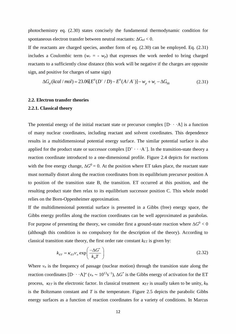
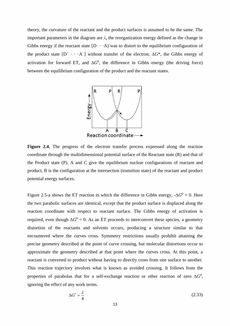
2.4. The progress of the electron transfer process expressed along the reaction

coordinate through the multidimensional potential surface of the Reactant state

(R) and that of the Product state (P). A and C give the equilibrium nuclear

configurations of reactant and product, B is the configuration at the intersection

(transition state) of the reactant and product potential energy surfaces ....................... 13

2.5. The intersections of the Gibbs energy surfaces of the reactant (R) state, [D...A],

and the product (P) state, [D+...A-]. (a): an electron transfer reaction with the

driving force, - G0 = 0; (b): the normal region where -G0 ; (c): the condition

of maximum rate constant where -G0 = and (d): the inverted region where -

G0 > ......................................................................................................................... 14

2.6. The electron transfer is said to be adiabatic (a) and diabatic (b). Hrp refers to the

electronic coupling energy defined by eq. (2.40) ......................................................... 17

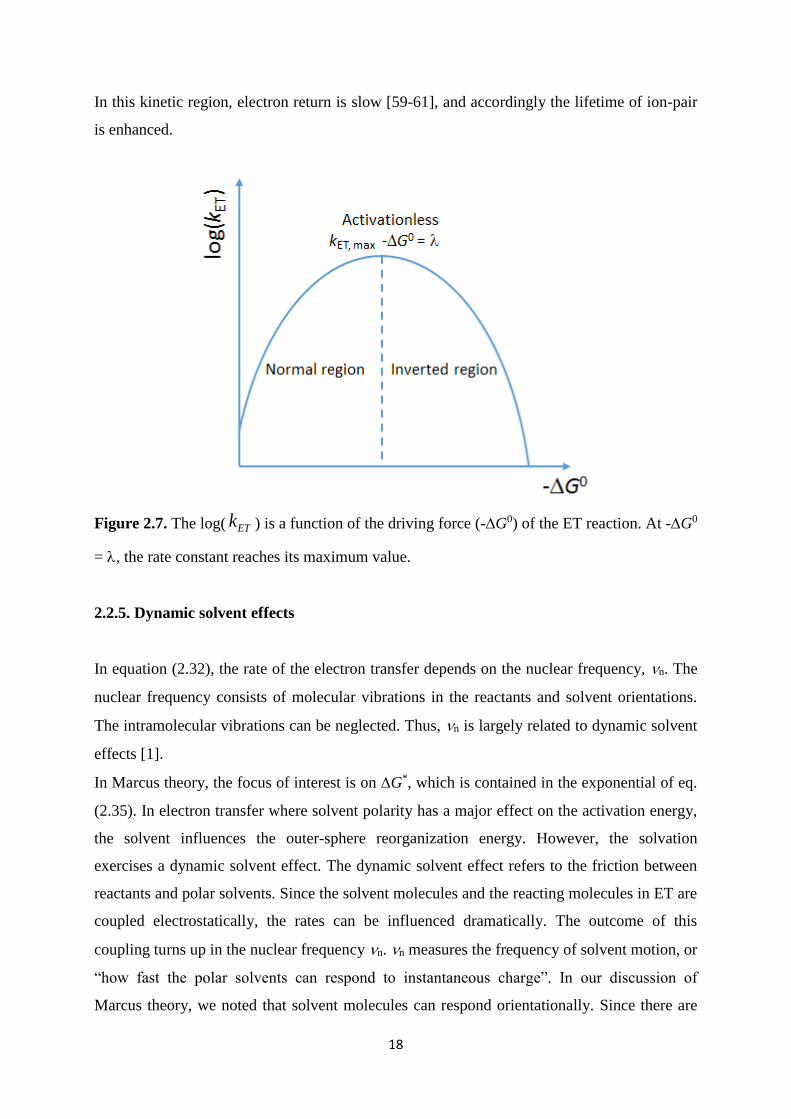
2.7. The log(kET ) is a function of the driving force (-G0) of the ET reaction. At -G0

= , the rate constant reaches its maximum value........................................................ 18

2.8. The parabolic curves: The top is a plot of G* vs. -G0. The energy potential

surfaces of the reactant and product shown in the bottom describe the

relationships between the driving forces (-G0) and reorganization energy ().

The normal region (-G0 < ) is shown on the left, G* decreases with decreasing

or as G0 becomes more negative. The inverted region (-G0 > ) is on the

right, G* increases with decreasing or as G0 becomes more negative. When

G* = 0, the rate is maximum (-G0 = ) and this case is shown in the center .......... 20

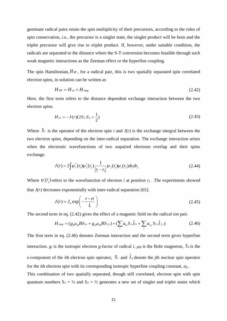
2.9. Vector presentation for the two electron spins of the spin correlated radical ion

pair in the presence of an external magnetic field. The precession of the electron

spin angular momentum vectors, Si, about the external magnetic field, Bz, is

included ........................................................................................................................ 23

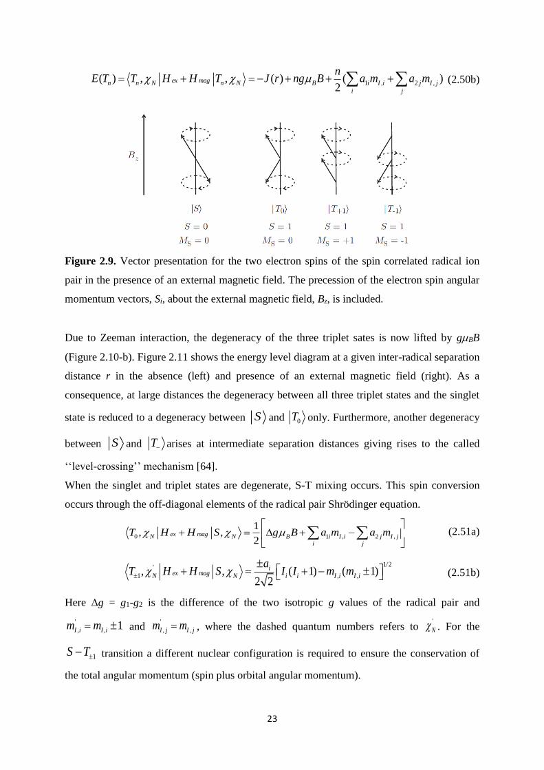
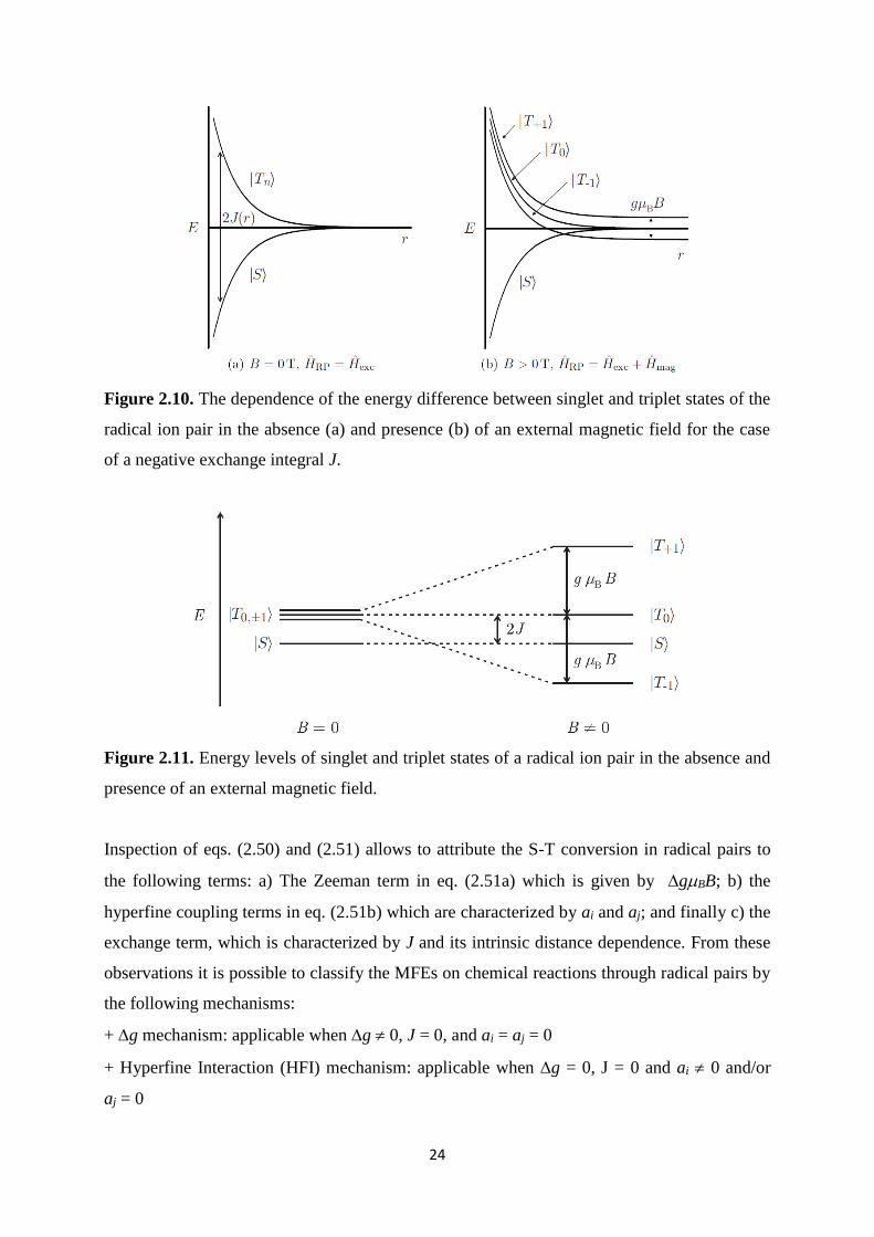
2.10. The dependence of the energy difference between singlet and triplet states of the

radical ion pair in the absence (a) and presence (b) of an external magnetic field

for the case of a negative exchange integral J .............................................................. 24

2.11. Energy levels of singlet and triplet states of a radical ion pair in the absence and

presence of an external magnetic field ......................................................................... 24

2.12. Vector model of the S-T0 conversion in a radical pair. The dephasing of the S1

and S2 spins which gives rise to the oscillatory S-T0 transition may be caused by

different g-value of the two radicals (g-mechanism) or by hyperfine interaction ..... 25

2.13. S-T conversion by g mechanism (a) and the dependence of the singlet

probability, S, on an external magnetic field (b) ........................................................ 26

2.14. Vector model of HFI induced S-T+ transition at zero magnetic field. The electron

spin, S1, and total nuclear spin, I, precess about their resultant and thereby change

their projections onto the z-axis ................................................................................... 27

2.15. S-T transition by the HFI-mechanism. At high field, the mixing occurs between

S and 0T since the 1T and 1T states are energetically split due to the Zeeman

interaction (here expressed in terms of the angular frequency 1

i Bg B ). At

low and zero external magnetic field the smaller energy gap between S and 1T

and 1T allows for transitions between singlet and all three triplet states .................. 27

2.16. Schematic representation of the species involved in the process of the magnetic

field effect on the exciplex of free acceptor/donor (a) and chain-linked

acceptor/donor (b) pairs: photoexcitation (1), exciplex formation (1A), direct

formation of the RIP via remote electron transfer (1B), exciplex dissociation into

RIP (2), spin evolution by hyperfine interaction (HFI), the singlet RIP re-forms

the exciplex (3) and exciplex emission (4). The red and blue arrows denote the

fluorescent decay process of either the photo-excited acceptor (magneto-

insensitive) or the exciplex (magneto-sensitive) that are observed in the

experiment. The magnetically sensitive species are enclosed in the frame. Spin

multiplicities are indicated by superscripts .................................................................. 29

2.17. The lifetime of sample is calculated from the slope of a plot of ln I(t) versus

time, t ............................................................................................................................ 31

2.18. TCSPC data for 1-bromo-8-[9-(10-methyl)anthryl]octane (MAnt-8-Br) in propyl

acetate. The green curve, L(tk), denotes the instrument response function. The blue

curve, N(tk), gives the measured data and the red curve, Nc(tk) is called the fitted

function. The lifetime of the fluorophore, , determined after fitting is 13 ns. The

upper panel shows some minor systematic error ......................................................... 33

3.1. Chemical structures of electron acceptors used in time-resolved magnetic field

effect studies ................................................................................................................. 35

3.2. Chemical structures of electron donors used in experiments ....................................... 36

3.3. Absorption and fluorescence spectra of Mant-10-O-2-DMA in a mixture of propyl

acetate/butyronitrile at s = 12. The fluorescence of the locally excited states and

the exciplex are shaded in blue and red, respectively .................................................. 43

3.4. (Upper panel) Emission time trace of the Mant-16-O-2-DMA exciplex in

butyronitrile (s = 24.7) in the absence (gray plot) and presence (red plot) of an

external magnetic field monitored with a 550 nm long-pass filter after excitation

with a laser pulse at 374 nm. Time-resolved magnetic field effect of the exciplex

extracted from the experimental data was shown in lower panel (blue plot) ............... 44

3.5. Scheme of the time-resolved magnetic field effect setup............................................. 45

4.1. The graphic visualization of the exciplex kinetics of inter-systems (left panel) and

Mant-n-O-2-DMA systems (right panel): I gives the probability of the initial

singlet radical ion pair (SRIP) formation while E = 1-I denotes the probability of

the initial exciplex formation. The exciplex dissociates into the singlet radical ion

pair with the rate constant, kd, the SRIP associates into the exciplex with the rate

constant, ka and the radiative/non-radiative exciplex decay to the ground-state

(GS) with the rate constant, 1

E . LE refers to the locally-excited acceptor .................. 46

4.2. Calculated singlet probability as a function of time for anthracene/N,N-

diethylaniline at zero field and high field limit. The solid lines denote pS (t) when

the electron self-exchange taken into account with ex = 8 ns whereas the dash

lines show pS(t) with neglecting the electron self-exchange ........................................ 50

5.1. The magnetic field effects on the inter-systems (a-c) and Mant-n-O-2-DMA

exciplexes (d-f) determined from TR-MFE using eq. (3.3) (filled circle with error

bars) and from steady-state measurements using eq (3.1) (open circles with error

bars) in propyl acetate/butyronitrile mixtures with varying the dielectric constant,

s. For intra-acceptor/donor systems, propionitrile (EtCN) and acetonitrile (ACN)

are used to extend the range of the solvent polarity ..................................................... 52

5.2. Magnetic field dependence of the exciplex fluorescence of polymethylene-linked

compounds (Mant-n-O-2-DMA) in neat butyronitrile. The MFEs on systems were

obtained in steady-state measurements by detecting the exciplex emission

intensity at 550 nm for 60 s, using a spectrometer time constant of 1 s. For each E

value, fluorescence intensities were acquired alternating three times between zero

and an external magnetic field. The data were analysed to extract the E values by

using eq. (3.1) ............................................................................................................... 53

5.3. Graphic visualization of S-T conversion in the zero field and an external field (B0

< 22 mT) for the linked-system of Mant-6-O-2-DMA ................................................ 54

5.4. Wavelength-resolved magnetic field effects of the Mant-n-O-2-DMA (n = 8, 10,

16) systems in butyronitrile. F and E denote the magnetic field effects on the

locally-excited fluorophore and the exciplex, respectively .......................................... 56

5.5. The exciplex emission bands of the studied inter-systems in propyl

acetate/butyronitrile mixture at s = 13 ........................................................................ 57

5.6. Exciplex fluorescence spectra of inter-systems (a-b) and Mant-n-O-2-DMA

systems (c-d) in neat propyl acetate (PA), butyronitrile (BN) and mixtures of

propyl acetate/butyronitrile (PA/BN) at different dielectric constants ........................ 59

5.7. Experimental (grey scatter plots) and simulated (red solid lines) time-dependent

magnetic field effects. The left column shows data for the anthracene/N,N-

diethylanline system at different s in propyl acetate/butyronitrile mixtures. The

right column illustrates for the 9-methylanthracene/N,N-diethylaniline system .......... 61

5.8. The driving force dependence of the TR-MFEs observed for the systems 9,10-

dimethylanthracene/N,N-dimethylaniline (-G0 0.28 eV), 9-

methylanthracene/N,N-diethylaniline (-G0 0.47 eV), and anthracene/N,N-

diethylaniline (-G0 0.58 eV) at s = 13 . The grey scatter plots denote the

experimentally time-resolved magnetic field effect data and their simulations are

given in the red solid lines............................................................................................ 62

5.9. Solvent polarity dependence of the exciplex lifetimes for the studied inter-systems .. 63

5.10. Solvent dependence of the dissociation rate constants for the studied inter-systems

...................................................................................................................................... 63

5.11. Solvent dependence of the initial probability of the loose ion pair state, I, (upper

panel) and the dissociation quantum yield of the exciplex, d, (lower panel) of the

systems 9,10-dimethylanthracene/N,N-dimethylaniline (red filled squares), 9-

methylanthracene/N,N-diethylaniline (grey filled triangles), and anthracene/N,N-

diethylaniline (blue filled circles) in propyl acetate/butyronitrile mixtures. The

sole purpose of the solid lines is to guide the eye; no physical model is implied ........ 64

A1. 1H, 13C-NMR and mass spectra of Mant-n-O-2-DMA compounds ............................. 74

A2. Absorption and fluorescence spectra of inter-systems and Mant-n-O-2-DMA

compounds in propyl acetate/butyronitrile mixture at s = 12 ..................................... 75

A3. From right to left of upper panels: The exciplex emission decays of the DMAnt

(2.10-5 M)/DMA (0.06 M) and MAnt (2.10-5 M)/DEA (0.06 M) in the absence and

presence of an external magnetic field, respectively. Lower panels: Time-resolved

magnetic field effects of the exciplexes extracted from the experimental data (gray

scatters) and simulations (red lines). Propyl acetate/butyronitrile mixture at s = 18

used as a solvent ........................................................................................................... 76

A4. Upper panels of (a) and (b): The exciplex emission decays of the Mant-8-O-2-

DMA (2.10-5 M) and Mant-10-O-2-DMA (2.10-5 M) in the absence and presence

of an external magnetic field, respectively. Lower panels of (a) and (b): Time-

resolved magnetic field effects of the exciplexes extracted from the experimental

data (gray lines). Neat butyronitrile (s = 24.7) used as a solvent ................................ 77

LIST OF TABLES

3.1. Physical parameters of the used acceptors and donors: The 0,0-energy E00,

lifetime of acceptors (A), A, and donors (D), D, reduction and oxidation

potentials, 𝑬𝟏/𝟐𝒓𝒆𝒅 and 𝑬𝟏/𝟐

𝒐𝒙 , respectively. The free energy difference of electron

transfer -G0 was calculated at s = 13 in propyl acetate/butyronitrile mixture,

using the Rehm-Weller equation with Born correction assuming an inter-particle

distance of 6.5 Å and an ion radius of 3.25 Å. ............................................................. 37

3.2. Chemicals were used in the synthetic steps of the polymethylene-linked

acceptor/donor systems. Abbreviations: Mant: 9-methylanthracene, 1,6-DBH: 1,6-

dibromohexane, 1,8-DBO: 1,8-dibromooctane, 1,10-DBD: 1,10-dibromodecane,

1,16-HDDO: 1,16-hexadecanediol, DMAPE: 2-[(4-

dimethylamino)phenyl]ethanol. Supplier and purification are indicated ..................... 39

3.3. Macroscopic solvent properties are given at 25 0C: density (), dielectric constant

(s), dynamic viscosity (), refractive index (n). Additionally the solvent supplier

and the purification methods are given. Abbreviations: PA: propyl acetate, BN:

butyronitrile, ACN: acetonitrile, EtCN: propionitrile .................................................. 40

3.4. The dielectric constant mixture (s, mix), mole fraction of butyronitrile (xBN),

viscosity (), refractive index (n) and Pekar factor ( = (1/n2 – 1/s) of PA/BN

mixtures ........................................................................................................................ 41

4.1. Used hyperfine coupling constants, Ha, for anthracene-. ............................................. 48

4.2. Used hyperfine coupling constants, Ha, for 9-methylanthracene-. ............................. 48

4.3. Used hyperfine coupling constants, Ha, for 9,10-dimethylanthracene-. ....................... 48

4.4. Used hyperfine coupling constants, Ha, for the radical cation of N,N-

diethylaninline+.. No experimental values are available, the values below have

been calculated using DFT (UB3LYB/EPRII)............................................................. 48

4.5. Used hyperfine coupling constants, Ha, for N,N-dimethylaniline+.. No

experimental values are available, the values below have been calculated using

DFT (UB3LYB/EPRII) ................................................................................................ 48

5.1. Some parameters of the studied A/D pairs at s = 13 in propyl acetate/butyronitrile

mixture. E00 is the 0-0 transition energy of acceptor; -GEx refers to the free

energy of exciplex formation; -GR gives the free energy of back-electron

transfer; max denotes the maximum wavelength of the exciplex emission band. ....... 58

ABSTRACT

This work is an approach based on the time-resolved magnetic field effect (TR-MFE) of the

delayed exciplex luminescence to distinguish the initial quenching products in fluorescence

quenching reactions via inter-and intra-molecular photo-induced electron transfer (ET)

between an electron excited acceptor (A*) and an electron donor (D). TR-MFEs based on the

Time-Correlated Single Photon-Counting (TCSPC) method of inter-and intra-acceptor/donor

exciplex emissions are measured in micro-homogeneous binary solvent mixtures of propyl

acetate/butyronitrile by varying the static dielectric constant, s, in a range from 6 to 24.7. For

free acceptor/donor pairs, the study focuses on the effects of the driving force of ET, -G0,

and the solvent polarity, s. In order to change -G0, the different free acceptor/donor pairs are

used with the -G0 varied in the range from 0.28 to 0.58 eV. Chain-linked acceptor/donor

pairs have been synthesized with varying the chain length to clarify the mechanism of

fluorescence quenching via intra-molecular photo-induced ET. All experimental data have

been analysed by using a model in which the reversibility of the exciplex and radical ion pair

(RIP) is taken into account.

ZUSAMMENFASSUNG

Im Ramen dieser Arbeit wurden versucht die primären Quenching-Produkte von Fluoreszenz-

Quenching Reaktionen auf Basis eines inter- oder intramoleklaren photoinduzierten

Elektronentransfers zwischen einem angeregten Elektronenakzeptor (A*) und einem

Elektronendonor (D) bestimmt. Dafür wurde mittels Time-Correlated-Single-Photon-

Counting (TCSPC) der zeitaufgelöste Magnet-Feld-Effekt (TR-MFE) der Lumineszenz des

Exiplex untersucht. Im Zentrum steht der Einfluss der Polarität des Lösungsmittel,

repräsentiert durch εs. Die Polarität des Lösungsmittels wurde mittels micro-heterogenen

binären Lösungsgemischen aus Propylacetat/Butyronitril variiert, wobei ein Bereich von 6–

24,7 für εs abgedeckt wurde. Als freie Akzeptor/Donor Paare wurde verschiedene Systeme

gewählt, sodass zusätzlich der Einfluss der Triebkraft der Reaktion -∆G0 untersucht werden

konnte. Es wurde ein Bereich von 0,28-0,58 eV abgedeckt. Um intramolektularen

photoinduzierten Elektronentransfer zu beobachten, wurden kovalent verbundene

Akzeptor/Donor Systeme synthetisiert, wobei die Länge der Verbrückung variiert wurde, um

den Einfluss dieser zu untersuchen. Alle Daten wurden mit einem Model analysiert, welches

Exiplex und Radikal Ionen Paar (RIP) als reversibel animmt.

ACKNOWLEDGEMENTS

I would like to thank many people for their patience and contribution to my thesis. I would

not finish without their help. The length of these acknowledgements is not enough to express

my gratitude and appreciation to them.

First, I’m deeply indebted to Dr. DANIEL KATTNIG who was, although not officially, my

second advisor. I’m astonished at his patience. He taught me everything concerning magnetic

field effect theory. With wide knowledge of literature, chemistry, numerical methods and

capability of explaining complex theory, he could always give detailed answers for all my

questions. Without his guidance and help to analyse the experimental data, I would not

definitely accomplish my dissertation. DANIEL! Thank you so much, my gratitude to you

will last forever.

I’m thankful to Prof. Dr. GÜNTER GRAMPP, my supervisor, who gave me the opportunity

to come to Austria. From whom, I learnt much about electron transfer and photochemistry

theories. His enthusiasm and the way of thinking are stimulating, which makes me more

confident in scientific discussion.

It is a pleasure to thank Assoc. Prof. Dr. Stephan Landgraf, who was willing to help me

adjusting and fixing the Single Photon Counting apparatus. I have gained the knowledge on

fast and modern kinetics from his lectures. Thanks for personal communication in magnetic

field effect results.

Many thanks to Dr. Kenneth Rasmussen, Dr. Boryana Mladenova Katting, who were

abundantly helpful in science for my work. Furthermore, you are my good friends for sharing

and helping.

I would like to thank all members of the Institute of Physical and Theoretical Chemistry, Graz

University of Technology. Special thanks to Eisenkölbl, Freißmuth, Ines, Hofmeister and

Lang. Thank you for solving apparatus problems and keeping things running.

I wish to thank my friends and colleagues at Prof. Grampp’s group. They gave me a great

atmosphere. Thanks for all the emotional support and entertainment.

Financial supports given by Vietnam International Education Development (VIED) and

Austrian Science Foundation, FWF-Project P 21518-N19 for my study are acknowledged.

Last but not at all least, Vân, Đăng and my family! Their supports help me to overcome

difficulties. Thank you so much for their endless love.

1

1. INTRODUCTION

Photo-induced electron transfer (ET) reactions have been extensively studied for many years.

This surge is motivated by the fact that ET is one the most fundamental, omnipresent

elementary reactions in chemistry, physics, and biochemistry [1-4]. However, questions about

the microscopic details of the quenching still remain, in particular in solvents of low

permittivity. In these media a photo-excited acceptor (A*) or a fluorophore (F*) diffusively

approaching a suitable electron donor (D) or a quencher (Q); or vice-versa, i.e. D could be

photo-excited, can be deactivated in a charge separation reaction either by forming a solvent-

separated, loose ion pair (LIP) or by the formation of an excited-state charge-transfer complex

(exciplex), which in the absence of intrinsic fluorescence emission is also referred to as a

contact ion pair (CIP). While the LIP is formed at distances longer than or equal to the contact

distance of A* and D, the exciplex formation typically involves tight stacking and a well-

defined relative orientation [5-9], which can be inferred from the correlated motion of the

quencher and the fluorophore in the complex [10]. The solvent permittivity strongly affects

the quenching mechanism. In polar solvents, quenching occurs predominantly by distant ET,

i.e. by an ET process yielding directly the LIP. However, in non-polar solvents (i.e., low

permittivity), exciplex fluorescence is often observed, suggesting the contribution of the

exciplex formation in the ET deactivation (the exciplexes can also result from secondary

recombination of initially formed ion-pairs; this question is addressed in the result discussion

section) [11-18]. Only a few exceptions to this empirical rule are known in the literature. E.g.,

a CIP is dominantly formed by diffusive ET quenching of 9,10-dicyanoanthracene (DCA) by

durene even in acetonitrile (quantum yield: 0.8) [19].

The primary quenching products are strongly affected by energetic parameters. The direct

formation of free ions, partly at distances exceeding the contact distance, is expected to be

significant for systems with larger driving force [10, 14, 20, 21]. The experimental results for

the DCA/durene system in acetonitrile indicated that with a free energy change of ion

formation of -G0 = 0.25 eV, exciplexes are formed efficiently in the bimolecular quenching

reaction from AD* state, whereas in the case of 2,6,9,10-tetracyanoanthracene

(TCA)/pentamethylbenzene (PMB) with -G0 = 0.75 eV, an exciplex could not be detected

[22, 23]. Exciplex fluorescence was observed for several systems in acetonitrile when

2

the -G0 is in the range from -0.28 to +0.20 eV [7, 8]. Yet, full electron transfer is observed

for the vast majority of donor-acceptor system in acetonitrile [7, 8, 13, 23, 24].

In general, exciplexes can be observed by their emission, which are, in the most favourable

cases, spectrally well separated from the locally excited fluorescence [11, 19, 23].

Furthermore, under suitable conditions, this exciplex emission is sensitive to an external

magnetic field [25-36].

In the literature dealing with MFE it is generally assumed that a LIP is formed initially and re-

combine irreversibly to an exciplex [32, 37-38]. Or the exciplex is an initial quenching

product even in polar environment [34, 39]. Unfortunately, no details about the mechanism of

fluorescence quenching reaction are known. In order to clarify the quenching mechanism via

ET, a model has been introduced in ref. 36. There, by systematically varying the bulk

dielectric constant, s, of micro-homogeneous binary solvents and using the model with the

reversibility between the exciplex and the LIP to simulate the experimental data. The initial

states of quenching, i.e., LIP (or radical ion pair-RIP) and exciplex based on the TR-MFEs of

the exciplex, have been discriminated.

All studies mentioned above depict the picture of the mechanism of fluorescence quenching

reaction via inter-molecular ET by bimolecular process. Intra-molecular photo-induced ET in

which acceptor/donor pair attached via a flexible chain is more complicated since, this

process relates to the dynamics of chain conformations. The competition between distant ET

and exciplex formation is dependent on solvent characteristics such as dielectric constant and

viscosity as well as structural features of the acceptor-spacer-donor system [40-43]. MFE

studies on intra-molecular exciplex fluorescence have been investigated. However, most of

these studies are generally mixing. The experimental data were discussed under the

assumption that the singlet radical ion pair (SRIP) is an initial quenching product and the

singlet exciplex (SE) is generated from SRIP recombination [33, 44-45] or focusing on the

dependence of the MFE on chain length [45].

This thesis contributes to a deeper and better understanding of the fluorescence quenching

mechanism via inter- and intra-molecular photo-induced ET. To investigate the effect of the

ET driving force (-G0) on the initial quenching products, the -G0 was varied in the range

from 0.28 to 0.58 eV by using different free acceptor/donor pairs. The polymethylene-linked

9-methylanthracene and N,N-dimethylaniline were synthesized to distinguish the primary

quenching products via intra-molecular photo-induced ET. Time-resolved magnetic field

effects of the exciplexes based on the time-correlated single photon-counting (TCSPC)

method have been measured in micro-homogeneous binary solvent of propyl

3

acetate/butyronitrile mixtures with the dielectric constant, s, varying from 6 to 24.7. The

experimental data have been simulated by the model in which the exciplex dissociation is

taken into account [36].

This thesis is organized as follows:

Theoretical considerations including theories of photo-induced electron transfer

(PET) reaction, magnetic field effects (MFE) of the exciplexes (time-resolved and

steady-state foundations), and Time-Correlated Single Photon Counting (TCSPC)

technique are summarized in chapter 2.

Time-resolved MFE measurements by using TCSPC technique, steady-state

measurements, the simulation model and the details in the solvent and sample

preparations are presented in chapter 3 and 4.

Chapter 5 presents the experimental data and their analysis.

Finally, some conclusions and outlooks to possible future work are presented in

chapter 6.

4

2. THEORETICAL BACKGROUND

2.1. Photo-induced electron transfer

2.1.1. Introduction

The relation between the rate constant of a chemical reaction, the activation energy and

thermal energy was introduced in 1889 by Svante Arrhenius [46] by an equation:

exp( )aEk A

RT

(2.1)

Where R is the gas constant, A is the pre-exponential factor or the frequency factor, and Ea

refers to the activation energy of the reaction. Both A and Ea are temperature dependent. The

reaction rate depends on the driving force and the activation energy. A transition state was

involved in Arrhenius equation. The aim of the transition state theory is to determine the

principal features governing the magnitude of a rate constant in terms of a model of the steps

that take place during the reaction. There are several approaches to the determination and

calculation, the simplest approach was introduced by Erying [47-49]. The final product was

generated via the formation of an activated complex, C‡, in a rapid pre-equilibrium with A, B

reactants.

A + B C Product (2.2)

The mostly used theory dealing with electron transfer (ET) is developed by Marcus [1-4]. The

detailed Marcus theory and the important expression will consider in the next section. Marcus

theory is used for the ET reaction between an excited electron acceptor (A*) and an electron

donor (D), called as the photo-induced electron transfer (PET) reaction. The ET process of the

acceptor/donor pair can proceed in three steps

Formation of the precursor complex: In the first step, the reactants diffusively approach

each other to form a precursor complex (the rate of formation of precursor complex usually

approaches diffusion-controlled limit).

* *[ ... ]diff

diff

k

kA D A D

(2.3)

Formation of the successor complex: In the second step, the electron transfer takes place at

transition state to generate a successor complex [A-…D+]* after the precursor complex

[A*…D] underwent reorganization towards a transition state.

5

* *[ ... ] [ ... ]ET

ET

k

kA D A D

(2.4)

Formation of free ions: In the final step, the successor complex dissociates to form the free

ions A- and D+.

*[ ... ] d

d

k

kA D A D

(2.5)

A steady-state treatment of equations (2.3) to (2.5) leads to the following kinetic expression of

the observed bimolecular electron transfer rate constant.

1 1 11 ET

q diff eq ET d

k

k k K k k

(2.6)

Where diff

eq

diff

kK

k

. If d ETk k

1 1 1 11

diff

q diff eq ET diff ET

k

k k K k k k

(2.7)

If the electron transfer rate is slow as compared to diffk ( ET diffk k ) then q eq ETk K k . When

ET diffk k we see that q diffk k and the rate of product formation is controlled by diffusion of

A* and D in solution.

2.1.2. Diffusion-controlled and electron transfer rate constants

The analysis is started with Scheme (2.8) with an assumption that the excited species is an

electron donor:

* * *[ ... ] [ ... ]diff ET d

diff ET

k k k

k kA D A D A D A D

(2.8)

diffk is the diffusion rate constant between reactants, diffk denotes the rate of separation of the

encounter complex, *[ ... ]A D , ETk is the first-order rate constant of electron transfer step. The

reverse step is designated by the rate constant ETk . The encounter complex lifetime is about

10-9 to 10-10s. During this time two molecules may undergo numerous collisions before they

react or separate from the encounter complex into the bulk of solvent molecules. In PET, an

encounter complex can be visualized as an ensemble consisting of a sensitizer and quencher

surrounded by solvents molecules (solvent shell). The sensitizer and quencher are said to be

contained within a solvent cage. For the spherical reactants within the solvent cage, the

center-to-center distance (dcc) is usually approximated around 7 Å. After the encounter

6

complex is formed, the sensitizer and quencher may undergo reaction or eventually escape

from the cage. If reaction takes place within the solvent cage, the ET products may revert

back to starting reactants, undergo irreversible chemical reaction, or leave the solvent cage by

ion dissociation. The rate of diffusion of two spherical reactants to an encounter distance

(assuming that dcc equals the sum of the reactant molecules’ radii) can be calculated from eq.

(2.9).

4diff AD cck D d (2.9)

Where DAD is the combined diffusion constant for approach of A and D. dcc is the center-to-

center distance. It suggests that the diffusion rate constant is the combined diffusion constant

and separation distance dependent. The Stokes-Einstein equation was used to calculate the

diffusion constant for one reactant.

6

Bk TD

r (2.10)

Where Bk is the Boltzmann constant, is the solution viscosity of the solution, and r is the

radius of the reactant. Introduction of eq. (2.10) into eq. (2.9) yields.

8

3

Bdiff

k Tk

(2.11)

Finally, using molar unit in eq. (2.11) gives a well-known version of the Smoluchowski

equation.

8

3000diff

RTk

(2.12)

For the fast ET reaction, i.e., reaction occurs at every collision after the reactants have already

been at encounter distance by diffusion. Thus ET diffk k and q diffk k (where qk is the rate of

quenching). Such reactions are diffusion controlled. According to eq. (2.12), a diffusion

controlled reaction (a fast quenching process) should depend on the temperature and the

viscosity of the solvent.

The bimolecular rate constant for the activated rate of electron transfer is defined as ak .

a eq ETk K k (2.13)

From eqs. (2.13) and (2.7) gives.

1 1 1

q diff ak k k (2.14)

7

qk is determined from Stern-Volmer measurements and diffk can be calculated from eq.

(2.12). From these two values, ak can easily be determined from eq. (2.14). In addition, the

equilibrium constant for the formation of the precursor complex, eqK can be expressed by

Norman Sutin [50].

24 exp rA A

wK N d d

RT

(2.15)

With the Coulombic work term given by

2

0

04 (1 )

A D Ar

s

z z e Nw

d d I

with

2

0

0

2 A

s B

N e

k T

Where NA is the Avogadro constant, A bd r r is the contact radius of the acceptor and donor

molecules, Ar and br are the mean molecular radii of acceptor and donor, d is reaction zone

thickness of roughly 0.8 Å, 0e id the elementary charge, I is the ionic strength of the solution,

Az and Dz are the charges of the acceptor and donor molecules, 0 is the vacuum permittivity

(or electric constant) and s is the static dielectric constant of the solvent.

With knowledge of ak , we can deduce a value for ETk from eq. (2.13).

If the radii and charges of the acceptor and the donor are different, the diffusion rate constant

is determined from the Debye equation [51].

2

0

0

2

0

0

44 ( )

exp 14

A D

s cc Bdiff A D cc A

A D

s cc B

z z e

d k Tk D D d N

z z e

d k T

(2.16)

and 1 1

6

BA D

A D

k TD D

r r

(2.17)

2.1.3. Energetics of photo-induced electron transfer

Photo-induced electron transfer was discussed in many literatures [52-55]. PET is a process

where an electron acceptor or an electron donor absorbs light to become an excited state. Due

to light absorption, some excited states act as strong electron acceptors and/or electron donors

8

depending on thermodynamic factors. The energetics is a crucial factor that determines the

feasibility of PET.

Ionization potentials and electron affinities of the excited state

The excited species containing a higher energy, have an important role on the donating or

accepting ability. Figure 2.1 shows the feasibility of the electron donating and electron

accepting processes of a ground state and an excited state. If the bound electron is expelled

from the orbital to an orbital within the continuum (E), the energy change associated with

this ejection is known as the ionization potential or IP which is the difference between the

orbital energy at infinite distances (E) and the energy of the lowest orbital (E1): (IP = E −

E1). The magnitude of IP is the energy required to ionize an atom or molecule (to remove an

electron from a molecule). The donating species is called an electron donor (D) (D → D+ + e−

+IPD). In the excited state, the excited electron placed a position in which the energy required

to eject it to the infinite distance is easier than the ground electron, i.e., the IP of an excited

state is less than the one of the ground state: IPD* = IPD – E00 where E00 is 0-0 transition

energy of donor. The energy released when the electron moves from the infinite distance to a

vacant orbital near nucleus is called the electron affinity or EA (A + e− → A− −EAA). The

accepting species is called an electron acceptor. In the excited state, there is a vacant orbital

which generated by light absorption, lying in lower energy level. Hence, the excited state

accepts an electron (A* + e− → A− −EAA*), the electron affinity (EAA*) of excited state is

greater than the one of the ground state EAA, (EAA* = EAA + E00). This model explains that

the ability of excited states act as better electron donor or acceptor.

Redox potentials of the excited state

The change enthalpy of the ionization of an electron donor in ground and excited states is

shown in the Figure 2.2. ∆𝐻𝐷→𝐷+ is positive quantity since it refers to an endothermic

process. While ∆𝐻𝐷∗→𝐷+ is more negative than ∆𝐻𝐷→𝐷+ by an amount equal to the energy of

the excited state (−∆𝐻𝐷∗→𝐷+ + ∆𝐻𝐷→𝐷+ = E00). The free energy change accompanying a

chemical process is G = H −TS. Where G is the free energy change between the

thermodynamic reactant and product states, S is the entropy of reaction and T is the absolute

temperature. The enthalpy change will be:

−∆𝐺𝐷∗→𝐷+ − 𝑇∆𝑆𝐷∗ →𝐷+ + ∆𝐺𝐷→𝐷+ + 𝑇∆𝑆𝐷→𝐷+ = 𝐸00 (2.18)

9

If assume that the structure of D and D+ and of D* and D+ are approximately the same, the

change in entropy is negligible. Thus, the free energy difference is G = H and ∆𝐺𝐷∗→𝐷+ =

∆𝐺𝐷→𝐷+ − 𝐸00.

The same arguments can be applied to evaluate the free energy changes for reduction of an

acceptor and its excited state with ∆𝐺𝐴∗→𝐴− = ∆𝐺𝐴→𝐴− − 𝐸00. The potential of a half

reaction, Eredox, is related to the free energy change by:

∆𝐺 = −𝑛𝐹𝐸𝑟𝑒𝑑𝑜𝑥 (2.19)

Where n gives the number of electron transfer, and F is a unit known as the Faraday constant.

Since Eredox is sensitive to the direction of the reaction, Eredox is sign dependent. A positive

Eredox implies an exothermic, spontaneous reaction and a negative value suggest an

endothermic process. In practice, when using Eredox whether it is oxidation or reduction, is

usually written as a reduction process.

Figure 2.1. The change of the ionization potential (IP) and electron affinity (EA) of an

excited state. The IP is decreased while the EA is released greater, as compared with the

ground state.

By convention 0( / )

D DE D D E

and *

0 *( / )D D

E D D E

, we write

0 * 0

00( / ) ( / )E D D E D D E (2.20)

According to eq. (2.20), the magnitude of E0(D+/D*) is now smaller than E0(D+/D), This

implies that the excited state is a better electron donor than the ground state. A similar

treatment can be applied to the reduction of A.

10

0 * 0

00( / ) ( / )E A A E A A E (2.21)

In this case, since its redox potential is more positive, the excited state is a better electron

acceptor than its ground state.

Figure 2.2. The enthalpy changes for formation of D+ from D and D* and for formation of A-

from A and A*.

Rehm-Weller equation

Having established thermodynamic relationships for deriving the redox potentials of

reductions and oxidations of excited state donor and acceptor molecules. A useful expression

for calculating the free energy change accompanying excited state electron transfer should be

derived. In Figure 2.3 depicts a thermodynamically uphill pathway involving D and A and a

downhill pathway from D* and A.

The overall free energy change for the uphill process is equal to the sum of the free energy

changes for oxidation of the donor and reduction of the acceptor.

el D D A AG G G

(2.22)

Where Gel gives the standard free energy change. Using eqs. (2.19) and (2.22) gives

( )el D D A AG nF E E

(2.23)

Using redox potentials.

0 0( ) [ ( / ) ( / )]elG eV nF E D D E A A (2.24)

A similar treatment for the ET between an excited donor and ground state acceptor, the free

energy change for this process is given by:

0 * 0( ) [ ( / ) ( / )]elG eV nF E D D E A A (2.25)

Substitution of eq. (2.20) into eq. (2.25) gives

11

0 0

00( ) [ ( / ) ( / ) ]elG eV nF E D D E A A G (2.26)

Where G00 (eV) is the free energy corresponding to E00. For most one electron transfers, nF

1, so that we can write

0 0

00( ) ( / ) ( / )elG eV E D D E A A G (2.27)

If we express the excited state in kilocalories per mole and redox potentials in volts, eq. (2.27)

becomes, for n = 1.

0 0

00( / ) 23.06[ ( / ) ( / ) ]elG kcal mol E D D E A A G (2.28)

If an electron acceptor is in an excited state (A*) and ET occurs between A* and D. A similar

treatment applied to this process also leads to eq. (2.28).

Figure 2.3. An energy diagram for photo-induced electron transfer.

The above expressions applied to the ET process between neutral acceptor and neutral donor.

The products are two charge species D+ and A-. When these ions formed, attractive

Coulombic forces will draw the two ions closer together and result in a release of energy. This

attraction is given by a work term, wp, derived from Coulomb’s law.

2( ) 332( )( / ) D A D A

p

cc s cc s

z z e z zw kcal mol

d d

(2.29)

Where D

z and A

z are the charges on the molecules, s is the static dielectric constant of the

solvent, and dcc is the center-to-center separation distance (Å) between the two ions.

Combining eqs. (2.28) and (2.29) yields:

0 0

00( / ) 23.06[ ( / ) ( / )]el pG kcal mol E D D E A A w G (2.30)

Equation (2.30) is called the Rehm-Weller equation [55]. According to the work term in Eq.

(2.30), the presence of electrostatic interaction between two ions should influence the free

energy change accompanying electron transfer. At the heart of electron transfer

12

photochemistry eq. (2.30) states concisely the fundamental thermodynamic condition for

spontaneous electron transfer between neutral reactants: Gel < 0.

If the reactants are charged species, another form of eq. (2.30) can be employed. Eq. (2.31)

includes a Coulombic term (wr = - wp) that expresses the work needed to bring charged

reactants to a sufficiently close distance (this work will be negative if the charges are opposite

sign, and positive for charges of same sign)

0 0

00( / ) 23.06[ ( / ) ( / )]el p rG kcal mol E D D E A A w w G (2.31)

2.2. Electron transfer theories

2.2.1. Classical theory

The potential energy of the initial reactant state or precursor complex [D· · ·A] is a function

of many nuclear coordinates, including reactant and solvent coordinates. This dependence

results in a multidimensional potential energy surface. The similar potential surface is also

applied for the product state or successor complex [D+ · · ·A−]. In the transition-state theory a

reaction coordinate introduced to a one-dimensional profile. Figure 2.4 depicts for reactions

with the free energy change, G0 = 0. At the position where ET takes place, the reactant state

must normally distort along the reaction coordinates from its equilibrium precursor position A

to position of the transition state B, the transition. ET occurred at this position, and the

resulting product state then relax to its equilibrium successor position C. This whole model

relies on the Born-Oppenheimer approximation.

If the multidimensional potential surface is presented in a Gibbs (free) energy space, the

Gibbs energy profiles along the reaction coordinates can be well approximated as parabolas.

For purpose of presenting the theory, we consider first a ground-state reaction where G0 < 0

(although this condition is no compulsory for the description of the theory). According to

classical transition state theory, the first order rate constant kET is given by:

expET ET n

B

Gk

k T

(2.32)

Where νn is the frequency of passage (nuclear motion) through the transition state along the

reaction coordinates [D· · ·A] (νn ∼ 1013s−1), G* is the Gibbs energy of activation for the ET

process, ET is the electronic factor. In classical treatment ET is usually taken to be unity, kB

is the Boltzmann constant and T is the temperature. Figure 2.5 depicts the parabolic Gibbs

energy surfaces as a function of reaction coordinates for a variety of conditions. In Marcus

13

theory, the curvature of the reactant and the product surfaces is assumed to be the same. The

important parameters in the diagram are λ, the reorganization energy defined as the change in

Gibbs energy if the reactant state [D· · ·A] was to distort to the equilibrium configuration of

the product state [D+ · · ·A−] without transfer of the electron; G*, the Gibbs energy of

activation for forward ET, and G0, the difference in Gibbs energy (the driving force)

between the equilibrium configuration of the product and the reactant states.

Figure 2.4. The progress of the electron transfer process expressed along the reaction

coordinate through the multidimensional potential surface of the Reactant state (R) and that of

the Product state (P). A and C give the equilibrium nuclear configurations of reactant and

product, B is the configuration at the intersection (transition state) of the reactant and product

potential energy surfaces.

Figure 2.5-a shows the ET reaction in which the difference in Gibbs energy, -G0 = 0. Here

the two parabolic surfaces are identical, except that the product surface is displaced along the

reaction coordinate with respect to reactant surface. The Gibbs energy of activation is

required, even though G0 = 0. As an ET proceeds to interconvert these species, a geometry

distortion of the reactants and solvents occurs, producing a structure similar to that

encountered where the curves cross. Symmetry restrictions usually prohibit attaining the

precise geometry described at the point of curve crossing, but molecular distortions occur to

approximate the geometry described at that point where the curves cross. At this point, a

reactant is converted to product without having to directly cross from one surface to another.

This reaction trajectory involves what is known as avoided crossing. It follows from the

properties of parabolas that for a self-exchange reaction or other reaction of zero G0,

ignoring the effect of any work terms.

4G

(2.33)

14

Figure 2.5. The intersections of the Gibbs energy surfaces of the reactant (R) state, [D...A],

and the product (P) state, [D+...A-]. (a): an electron transfer reaction with the driving force, -

G0 = 0; (b): the normal region where -G0 ; (c): the condition of maximum rate constant

where -G0 = and (d): the inverted region where -G0 > .

Figure 2.5-b depicts the ET reaction where -G0 0. The parabolic surface of the product,

[D+ · · ·A−] shifts vertically by G0 with respect to [D· · ·A] one. The activation energy for

the ET process is given by:

0 2( )

4

GG

(2.34)

Inserting eq. (2.34) into equation (2.32) yields the classical Marcus equation:

0 2( )exp

4ET ET n

B

Gk

k T

(2.35)

Equations. (2.34) and (2.35) and Figure 2.5 indicate that for the exergonic reactions, G* will

decrease and kET will consequently increase as G0 becomes more negative. When −G0 = λ

(Figure 2.5-c), G* = 0 and kET reaches it maximum value of κETνn. However, as G0

becomes more negative in a highly exergonic reaction, the intersection point of the R and P

15

surfaces moves to left of the center of the R surfaces as shown in Figure 2.5-d. G* should

increase again and thus, from the eq. (2.35), kET will decrease as the reaction becomes highly

exergonic in what has been called the Marcus Inverted Region.

2.2.2. Reorganization energy

The total reorganization energy, , is usually divided into two terms,

in out (2.36)

Where in is the inner-sphere reorganization energy and out is the outer-sphere

reorganization energy. Inner-sphere reorganization energy refers to the energy changes

accompanying changes in bond lengths and bond angles during electron transfer step. Outer-

sphere reorganization energy is the energy change as the solvent shells surrounding the

reactants rearrange.

The energy associated with changes in bond lengths (the inner-sphere reorganization energy)

is given by the following equation [56]:

2( ) ( )

( ) ( )

i iin i

i i i

f R f Pq

f R f P

(2.37)

Where iq is the difference in equilibrium bond distance between the reactant and product

states corresponding to a ith vibration, and f(R) and f(P) are the force constants for this

vibration for a reactant and product molecule. The quantity contained in brackets is referred

to as the reduced force constant. Equation (2.37) includes the summation of all vibrational

modes and applies to the limit case where all vibrational states (assumed to display harmonic

behaviour) are populated. This latter condition represents a case where in is assumed to be

temperature independent.

Solvent reorganization denotes the effects of orientational changes in the solvent molecules

surrounding the reactants during electron transfer. In this section we show that solvent plays a

special role in establishing the unique nature of the transition state in electron transfer. The

reorganization due to the solvent contribution is closely related to the polarization of the

solvent molecules surrounding a reactant pair. The solvent polarization is the sum of an

orientational-vibrational and an electronic component [57]:

e uP P P (2.38)

P is the total polarization, Pe is the electronic polarization, and Pu is the orientational-

vibrational polarization of the solvent molecules. Pe is associated with the optical dielectric

16

constant, op, which is in turn equal to the square of the refractive index, n2. Pu is associated

with the static dielectric constant, s. Pu, unlike Pe, responds more slowly at a much lower

frequency with an oscillating electric field.

The outer-sphere reorganization energy is given by the following expression:

2 1 1 1 1 1( / ) 332out

D A cc op s

kcal mol er r d

(2.39)

Where e is the charge transferred in the reaction, rD and rA are the radii of the donor and the

acceptor, respectively and dcc is the center-to-center distance between the donor and acceptor.

2.2.3. Adiabatic versus diabatic electron transfer reaction

The magnitude of the electronic coupling energy, Hrp, between the reactant and the product

states is used to distinguish the two types of ET reaction.

𝐻𝑟𝑝 = ⟨𝑅0 |Ĥ𝐸𝑇|

𝑃0 ⟩ (2.40)

Where 0

R and 0

P are the electronic wave functions of the equilibrium reactant and product

states, respectively and Ĥ𝐸𝑇 is the Born-Oppenheimer (rigid nuclei) electronic Hamiltonian

for the system. The ET reactions is said to be adiabatic if Hrp is moderately large, so that the

Gibbs energy surface interact as shown in Figure 2.6-a. Because the surfaces are separated in

the intersection region, the reaction always remains on the lower surface as it proceeds

through the transition state and the transmission coefficient κET ≃ 1 in eq. (2.35). When Hrp

becomes so small that the R and P surfaces no longer interact significantly, the ET reaction is

said to be diabatic. As indicated in Figure 2.6-b, the system will then usually remains on the

[D· · ·A] surface as it passes through the intersection region and will return to the equilibrium

state of reactant. Only occasionally it cross over to P surface, bring about the ET reaction. The

point at which a reaction is to be regarded as adiabatic or diabatic varies with system.

Adiabatic reactions are generally found in those cases in which D and A are relatively close

together. In practice this means either van der Waals contact of D and A in the reactant state

or close coupling of D and A in an intramolecular entity.

17

Figure 2.6. The electron transfer is said to be adiabatic (a) and diabatic (b). Hrp refers to the

electronic coupling energy defined by eq. (2.40).

2.2.4. Inverted region

Mathematically, equation. (2.34) describes a quadratic relationship between the driving force

and the free energy of activation. The physical meaning of this relationship will become

apparent if we take a closer look at the rate constants (eq. (3.35)) of an excited state

interacting with a series of homologous quenchers by an electron transfer mechanism [58]. If

the log(kET) is plotted vs. the driving forces (-G0) , the Figure 2.7 describes the following

trend: initially the rate will increase with an increase (more negative) in driving force and

reach the maximum value in which -G0 = . With further increases in the driving force, the

rate constant should progressively decrease again.

Figure 2.8 shows the intersecting reactant and product potential energy surfaces. Starting with

reactant and product curves (a), with increasing exothermicities, the activation energy

progressively decreases until at some point it reaches zero (b). Here the rate attains its

maximum value. With further increasing n the driving forces, the activation energy begins to

increase again (c).

In photo-induced ET, the inverted region has important implications in charge separation and

electron return. By taking advantage of the relationship, -G0 = , one might be able control

the onset of the inverted region for either forward ET or electron return and thereby influence

reaction. If, for example, the reaction is dominated by the effects of solvent rather than bond

reorganization, out. By varying the solvent, it is possible to change out. Let us say that

we want to increase the lifetimes of ion-pair intermediates by slowing the rate of electron

return. We chose a solvent so that 0G . This places the reaction in the inverted region.

18

In this kinetic region, electron return is slow [59-61], and accordingly the lifetime of ion-pair

is enhanced.

Figure 2.7. The log( ETk ) is a function of the driving force (-G0) of the ET reaction. At -G0

= , the rate constant reaches its maximum value.

2.2.5. Dynamic solvent effects

In equation (2.32), the rate of the electron transfer depends on the nuclear frequency, n. The

nuclear frequency consists of molecular vibrations in the reactants and solvent orientations.

The intramolecular vibrations can be neglected. Thus, n is largely related to dynamic solvent

effects [1].

In Marcus theory, the focus of interest is on G*, which is contained in the exponential of eq.

(2.35). In electron transfer where solvent polarity has a major effect on the activation energy,

the solvent influences the outer-sphere reorganization energy. However, the solvation

exercises a dynamic solvent effect. The dynamic solvent effect refers to the friction between

reactants and polar solvents. Since the solvent molecules and the reacting molecules in ET are

coupled electrostatically, the rates can be influenced dramatically. The outcome of this

coupling turns up in the nuclear frequency n. n measures the frequency of solvent motion, or

“how fast the polar solvents can respond to instantaneous charge”. In our discussion of

Marcus theory, we noted that solvent molecules can respond orientationally. Since there are

19

other solvent motions such as vibrational motions, the time required for solvation may span

several time scales. However, it is convenient to consider only the orientational motion of

solvent molecules. There may be a certain slowness associated with these motions, which

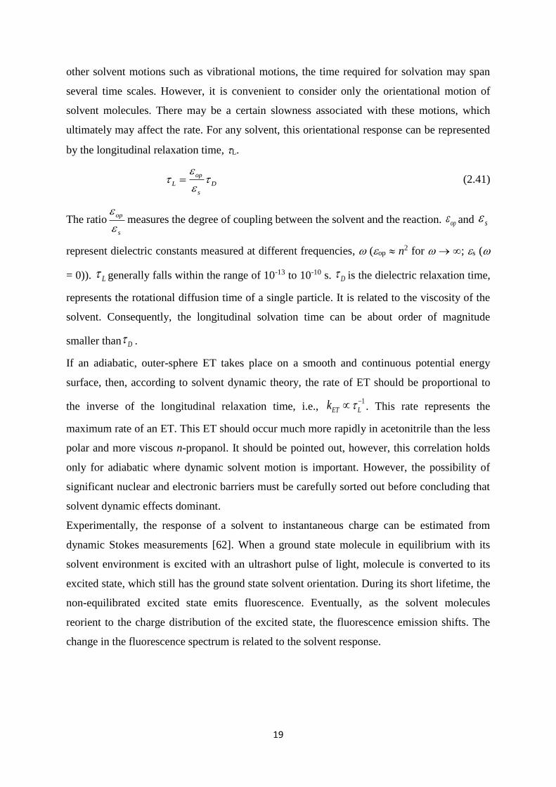
ultimately may affect the rate. For any solvent, this orientational response can be represented

by the longitudinal relaxation time, L.

op

L D

s

(2.41)

The ratioop

s

measures the degree of coupling between the solvent and the reaction. op and s

represent dielectric constants measured at different frequencies, (op n2 for ; s (

= 0)). L generally falls within the range of 10-13 to 10-10 s. D is the dielectric relaxation time,

represents the rotational diffusion time of a single particle. It is related to the viscosity of the

solvent. Consequently, the longitudinal solvation time can be about order of magnitude

smaller than D .

If an adiabatic, outer-sphere ET takes place on a smooth and continuous potential energy

surface, then, according to solvent dynamic theory, the rate of ET should be proportional to

the inverse of the longitudinal relaxation time, i.e., 1

ET Lk . This rate represents the

maximum rate of an ET. This ET should occur much more rapidly in acetonitrile than the less

polar and more viscous n-propanol. It should be pointed out, however, this correlation holds

only for adiabatic where dynamic solvent motion is important. However, the possibility of

significant nuclear and electronic barriers must be carefully sorted out before concluding that

solvent dynamic effects dominant.

Experimentally, the response of a solvent to instantaneous charge can be estimated from

dynamic Stokes measurements [62]. When a ground state molecule in equilibrium with its

solvent environment is excited with an ultrashort pulse of light, molecule is converted to its

excited state, which still has the ground state solvent orientation. During its short lifetime, the

non-equilibrated excited state emits fluorescence. Eventually, as the solvent molecules

reorient to the charge distribution of the excited state, the fluorescence emission shifts. The

change in the fluorescence spectrum is related to the solvent response.

20

Figure 2.8. The parabolic curves: The top is a plot of G* vs. -G0. The energy potential

surfaces of the reactant and product shown in the bottom describe the relationships between

the driving forces (-G0) and reorganization energy (). The normal region (-G0 < ) is

shown on the left, G* decreases with decreasing or as G0 becomes more negative. The

inverted region (-G0 > ) is on the right, G* increases with decreasing or as G0 becomes

more negative. When G* = 0, the rate is maximum (-G0 = ) and this case is shown in the

center.

2.3. Magnetic field effects

The present part will focus on the radical pair mechanism to explain the mechanism of the

magnetic field effects (MFEs) on chemical [63, 64]. There is an inspection of the two spin-

mixing mechanisms, including the hyperfine-mechanism and the g-mechanism. The effect

of the radical pair mechanism at intermediate fields on chemical reactions within the low-

viscosity approximation will be addressed. Finally, the photo-induced ET reaction scheme and

MFE on the exciplex emission will be described.

2.3.1. Radical pair mechanism

Radical pairs are generated via photo-induced electron transfer reactions of excited

fluorophores with quenchers. The spin multiplicity [singlet (S) or triplet (T)] of the correlated

21

geminate radical pairs retain the spin multiplicity of their precursors, according to the rules of

spin conservation, i.e., the precursor is a singlet state, the singlet product will be born and the

triplet precursor will give rise to triplet product. If, however, under suitable condition, the

radicals are separated to the distance where the S-T conversion becomes feasible through such

weak magnetic interactions as the Zeeman effect or the hyperfine coupling.

The spin Hamiltonian, RPH , for a radical pair, this is two spatially separated spin correlated

electron spins, in solution can be written as

RP ex magH H H (2.42)

Here, the first term refers to the distance dependent exchange interaction between the two

electron spins.

1 2

1( )(2 . )

2exH J r S S (2.43)

Where iS is the operator of the electron spin i and J(r) is the exchange integral between the

two electron spins, depending on the inter-radical separation. The exchange interaction arises

when the electronic wavefunctions of two unpaired electrons overlap and their spins

exchange.

* *

1 1 2 2 2 1 1 2 1 2

1 2

1( ) 2 ( ) ( ) ( ) ( )J r r r r r drdr

r r

(2.44)

Where ( )i jr refers to the wavefunction of electron i at position rj . The experiments showed

that J(r) decreases exponentially with inter-radical separation [65].

0( ) expr

J r JL

(2.45)

The second term in eq. (2.42) gives the effect of a magnetic field on the radical ion pair.

1 21 2 1 21 2 1 2( ) ( . . )mag i jz zB B i j

i i

H g BS g BS a S I a S I (2.46)

The first term in eq. (2.46) denotes Zeeman interaction and the second term gives hyperfine

interaction. gi is the isotropic electron g-factor of radical i, B is the Bohr magneton, izS is the

z-component of the ith electron spin operator, iS and ijI denote the jth nuclear spin operator

for the ith electron spin with its corresponding isotropic hyperfine coupling constant, aij .

This combination of two spatially separated, though still correlated, electron spin with spin

quantum numbers S1 = ½ and S2 = ½ generates a new set of singlet and triplet states which

22

can be expressed via the product of their individual electron ( X ) and nuclear spin ( i )

wavefunctions

1 2 1 2

1( )

2S (2.47a)

0 1 2 1 2

1( )

2T (2.47b)

1 1 2T (2.47c)

1 1 2T (2.47d)

Where and denote the parallel (spin-up, ms = +1/2) and antiparallel (spin-down, ms = -

1/2) magnetic substates of the electron in the presence of an external magnetic field, Bz,

respectively. Figure 2. 9 depicts the vector representation for the two electron spins of the

geminate radical ion pair in the presence of an external magnetic field, Bz. The overall spin

quantum number, S = 0, 1, and magnetic spin quantum number, Ms = -1, 0, 1, for the

correlated spin pair are indicated. The nuclear spin wavefunctions are given by:

, ,

a b

N I i I j

i j

m m (2.48)

Here ,I im and ,I jm refer to the magnetic nuclear spin quantum numbers on atom i of radical 1

and atom j of radical 2.

In the presence of an external magnetic field, the energies of the S and T states of the radical

ion pair are given by:

( ) , , ( )exN NE S S H S J r (2.49a)

( ) , , ( )exn n N n NE T T H T J r (2.49b)

With n = -1, 0, +1 for the three triplet states, 1T , 0T , 1T , respectively. The distance

dependence of the exchange integral ( )J r expresses the S and T energies distance dependence

as well.

The S and T energies are shown in Figure 2.10. Figure 2.10-a shows the S and T energies in

the absence of an external magnetic field. The energy gap is separated at close inter-radical

distances r and it becomes smaller at large separation distances. In the presence of an external

magnetic field, the singlet and triplet energies are given by:

( ) , , ( )ex magN NE S S H H S J r (2.50a)

23

1 , 2 ,( ) , , ( ) ( )2

ex magn n N n N B i I i j I j

i j

nE T T H H T J r ng B a m a m (2.50b)

Figure 2.9. Vector presentation for the two electron spins of the spin correlated radical ion

pair in the presence of an external magnetic field. The precession of the electron spin angular

momentum vectors, Si, about the external magnetic field, Bz, is included.

Due to Zeeman interaction, the degeneracy of the three triplet sates is now lifted by gBB

(Figure 2.10-b). Figure 2.11 shows the energy level diagram at a given inter-radical separation

distance r in the absence (left) and presence of an external magnetic field (right). As a

consequence, at large distances the degeneracy between all three triplet states and the singlet

state is reduced to a degeneracy between S and 0T only. Furthermore, another degeneracy

between S and T arises at intermediate separation distances giving rises to the called

‘‘level-crossing’’ mechanism [64].

When the singlet and triplet states are degenerate, S-T mixing occurs. This spin conversion

occurs through the off-diagonal elements of the radical pair Shrödinger equation.

0 1 , 2 ,

1, ,

2ex magN N B i I i j I j

i j

T H H S g B a m a m

(2.51a)

1/2'

1 , ,, , ( 1) ( 1)2 2

iex magN N i i I i I i

aT H H S I I m m

(2.51b)

Here g = g1-g2 is the difference of the two isotropic g values of the radical pair and

'

, , 1I i I im m and '

, ,I j I jm m , where the dashed quantum numbers refers to '

N . For the

1S T transition a different nuclear configuration is required to ensure the conservation of

the total angular momentum (spin plus orbital angular momentum).

24

Figure 2.10. The dependence of the energy difference between singlet and triplet states of the

radical ion pair in the absence (a) and presence (b) of an external magnetic field for the case

of a negative exchange integral J.

Figure 2.11. Energy levels of singlet and triplet states of a radical ion pair in the absence and

presence of an external magnetic field.

Inspection of eqs. (2.50) and (2.51) allows to attribute the S-T conversion in radical pairs to

the following terms: a) The Zeeman term in eq. (2.51a) which is given by gBB; b) the

hyperfine coupling terms in eq. (2.51b) which are characterized by ai and aj; and finally c) the

exchange term, which is characterized by J and its intrinsic distance dependence. From these

observations it is possible to classify the MFEs on chemical reactions through radical pairs by

the following mechanisms:

+ g mechanism: applicable when g 0, J = 0, and ai = aj = 0

+ Hyperfine Interaction (HFI) mechanism: applicable when g = 0, J = 0 and ai 0 and/or

aj = 0

25

Additionally, other mechanisms, such as the relaxation mechanism, spin-orbit coupling, or the

level crossing mechanism can induce S-T conversion in radical pairs. However, these three

mechanisms are not at all important for the freely diffusing, no heavy atoms containing,

radical pairs studied in the present work.

g mechanism

When the two electronic spins on the two radicals possess different g-values. As a

consequence their Larmor frequencies, 1

i i Bg B , with which they precess about the

external magnetic field effect, giving rise to a dephasing of the precessing of S1 and S2 with

respect to each other (Figure 2.12). As a result the spin multiplicity will oscillate between

S and 0T with the frequency.

0

1 1

1 2 1 2( )ST B Bg g B g B (2.52)

Figure 2.13-a gives a schematic representation of S-T conversion by g mechanism. This

mechanism induces a S-T conversion only in the presence of an external magnetic field, B

through the Bg B term in eq. (2.51a). Due to Zeeman interaction, the 1T and 1T states are

lifted energetically remove from the S state. Thus there is no mixing between S state and

T .

Figure 2.12. Vector model of the S-T0 conversion in a radical pair. The dephasing of the S1

and S2 spins which gives rise to the oscillatory S-T0 transition may be caused by different g-

value of the two radicals (g-mechanism) or by hyperfine interaction.

26

The dependence of the singlet probability, S, on an external magnetic field is depicted in

Figure 2.13-b, for a short lived radical pair, created in its singlet state, where spin evolution

can occur only to some small extent. The increasing importance of the g-mechanism at high

external magnetic fields, resulting in a reduction of the singlet probability, is obvious.

Figure 2.13. S-T conversion by g mechanism (a) and the dependence of the singlet

probability, S, on an external magnetic field (b).

Hyperfine Interaction mechanism

The electron-nuclear hyperfine interaction (HFI) induces S-T transitions qualitatively

different depending on the external applied magnetic field. At applied magnetic fields which

exceed the magnetic field, which is induced by the magnetic nuclei of the radical at the

location of the unpaired electron spin (B > 10 to 100 mT), the HFI-mechanism operates in a

way similar to the g-mechanism. Now, the HFI has the effect of an additional local magnetic

field that alters the precession frequency of the electronic spin (see Figure 2.12). The

electronic spin on the two radicals will have different local fields resulting in different

precession frequencies, which then induce spin conversion. Contrary to the g-mechanism,

the S-T transition rate is magnetic field independent. The large Zeeman splitting at high

external magnetic fields renders the S-T0 transition the only feasible mixing channel (see

Figure 2.51-a).

Generally the unpaired electron precesses about a magnetic field, Btot, which is the vector sum

of the external magnetic field, Bext, and the local hyperfine field, BHFI. Whenever Bext >> BHFI

the directions of Btot and Bext practically coincide, and hence the electron spin projection onto

the external field is not altered. In low external fields, however, Btot and Bext don not coincide

27

and thus the precess about Btot affects the spin projection onto Bext giving rise to transition

from S to all three T states. Figure 2.14 describes the situation for zero external field and

static electron spin on radical 2. The S-T transition occurs in the course of the precession of

the unpaired electron spin S1 and the nuclear spin I about their resultant (transitions to the

other two triplet states occurs in completely analogous way).

Figure 2.14. Vector model of HFI induced S-T+ transition at zero magnetic field. The electron

spin, S1, and total nuclear spin, I, precess about their resultant and thereby change their

projections onto the z-axis.

Figure 2.15. S-T transition by the HFI-mechanism. At high field, the mixing occurs between

S and 0T since the 1T and 1T states are energetically split due to the Zeeman interaction

(here expressed in terms of the angular frequency 1

i Bg B ). At low and zero external

magnetic field the smaller energy gap between S and 1T and 1T allows for transitions

between singlet and all three triplet states.

28

2.3.2. Magnetic field effects in view of the low viscosity approximation

The magnetic field effect (MFE), , is defined as the difference in the yield of a given species

in reaction such as radical ions, triplets, exciplexes, etc., in the presence, (B), and absence,

(B0), of an external magnetic field divided by the product yield at zero field.

0

0

( ) ( )

( )

B B

B

(2.53)

The low viscosity approximation includes the following two simplifications:

a) The exchange interaction is negligible, i.e., it is assumed zero over the entire domain of

spatial diffusion.

b) The diffusional evolution of the radical pair, n(r, t), and its spin evolution given by the

singlet probability, S(B, t), are treated independently (see the experimental section).

The product yield for species i is hence given as the integral of the singlet or triplet

probability of this species, i(B, t), weighted by a suitable function f(t), which describes the

species’ formation:

0

( , ) ( )i i B t f t dt

(2.54)

2.3.3. Photo-induced electron transfer reaction scheme and time-resolved magnetic field

effect of exciplex emission

Exciplexes appear as intermediate species in photochemistry. In general, exciplexes can be

observed by their emission. Furthermore, under suitable conditions, the exciplex production is

sensitive to an external magnetic field [25-36]. MFEs on exciplexes result from the inter-

conversion of the singlet and the three triplet states of the RIP in equilibrium with the

exciplex. This process is sensitive to the presence of an external magnetic field which lifts the

degeneracy of the three triplet states and, thus, reduces the singlet-triplet conversion (S-T+-).

This causes an increase of the singlet population of the initial spin state in the presence of a

magnetic field. Due to the reversible conversion of the exciplex and the singlet RIP, the

exciplex luminescence becomes magnetosensitive. Figure 2.16 depicts a reaction scheme of

the photo-induced ET processes of an exciplex forming donor-acceptor system. The involved

species can be classified by their inter-particle distance and the solvent polarization expressed

by the Marcus outer-sphere ET coordinate. Here, the horizontal arrangement is arbitrary.

29

(a) Free acceptor/donor pair

(b) Chain-linked acceptor/donor pair

Figure 2.16. Schematic representation of the species involved in the process of the magnetic

field effect on the exciplex of free acceptor/donor (a) and chain-linked acceptor/donor (b)

pairs: photoexcitation (1), exciplex formation (1A), direct formation of the RIP via remote

electron transfer (1B), exciplex dissociation into RIP (2), spin evolution by hyperfine

interaction (HFI), the singlet RIP re-forms the exciplex (3) and exciplex emission (4). The red

and blue arrows denote the fluorescent decay process of either the photo-excited acceptor

(magneto-insensitive) or the exciplex (magneto-sensitive) that are observed in the experiment.

The magnetically sensitive species are enclosed in the frame. Spin multiplicities are indicated

by superscripts.

Magnetic field effect on exciplex can proceed as following: An electron acceptor (A) in

ground state absorbs light to become an excited state (A*). The excited state is quenched via

electron transfer (ET) with an electron donor (D) in a process called as photo-induced electron

transfer (PET) reaction. In the course of the quenching process via ET, the two initial

quenching products are possible (1A versus 1B). The singlet radical ion pair (RIP) can be

formed via distant ET (1B) or by the dissociation of an exciplex (2), which is formed via

reaction (1A). The singlet RIP so obtained can undergo inter-system crossing induced by the

30

hyperfine coupling interaction and the Zeeman interaction. By applying an external magnetic

field, because of the Zeeman interaction, the singlet S and T states are not degenerate.

There is only S-T0 transition, this causes an increase in the singlet probability. Only the

singlet RIP can reform the exciplex and, thus, its formation and emission can be influenced by

an external magnetic field. Furthermore, since exciplex dissociation is a typically slow

process, the ions resulting from the exciplex dissociation will be delayed with respect to those

formed by direct electron transfer. As a consequence the MFE generated by the exciplex route

will also be delayed. Thus, time-resolved studies of MFE of the exciplexes, allow deducing

the initial quenching state (i.e., 1A versus 1B in Figure 2.16).

It is now possible to reformulate the magnitude of magnetic field effect introduced in eq.

(2.53) by taking the exciplex quantum yield as the observable species of interest,

0

0

( ) ( )

( )

exc exc exc

exc exc

B B

B

(2.55)

Here ( )exc B and 0( )exc B give the exciplex quantum yield in the presence and absence of an

external magnetic field, respectively. Within the low-viscosity approximation the numerator

can be expressed as:

0

0

( )( ( , ) ( , ))exc S Sf t B t B t dt

(2.56)

Here S refers to the singlet probability-as only the singlet RIP is capable of forming the

exciplex and ( )f t represents a recombination function describing the reformation of the

exciplex. Assuming, that the radical ion pair only decays via the exciplex, the quantum yield

of the exciplex can be expressed as:

1exc ions (2.57)

With ions giving the yield of free ions (or the survival probability of the radical pair at infinite

time).

2.4. Theory of experiments

2.4.1. Meaning of the lifetime in time-correlated single photon-counting (TCSPC)

technique

The time-domain and frequency-domain methods are widely employed to measure time-

resolved fluorescence [66]. In time-domain, the sample is excited with a pulse of light (Figure

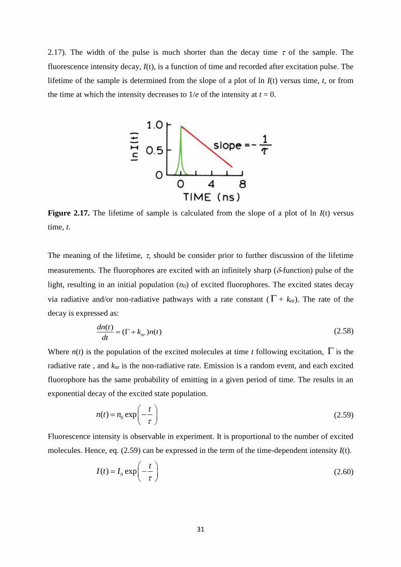
31

2.17). The width of the pulse is much shorter than the decay time of the sample. The

fluorescence intensity decay, I(t), is a function of time and recorded after excitation pulse. The

lifetime of the sample is determined from the slope of a plot of ln I(t) versus time, t, or from

the time at which the intensity decreases to 1/e of the intensity at t = 0.

Figure 2.17. The lifetime of sample is calculated from the slope of a plot of ln I(t) versus

time, t.

The meaning of the lifetime, , should be consider prior to further discussion of the lifetime

measurements. The fluorophores are excited with an infinitely sharp (-function) pulse of the

light, resulting in an initial population (n0) of excited fluorophores. The excited states decay

via radiative and/or non-radiative pathways with a rate constant ( + knr). The rate of the

decay is expressed as:

( )( ) ( )nr

dn tk n t

dt (2.58)

Where n(t) is the population of the excited molecules at time t following excitation, is the

radiative rate , and knr is the non-radiative rate. Emission is a random event, and each excited

fluorophore has the same probability of emitting in a given period of time. The results in an

exponential decay of the excited state population.

0( ) expt

n t n

(2.59)

Fluorescence intensity is observable in experiment. It is proportional to the number of excited

molecules. Hence, eq. (2.59) can be expressed in the term of the time-dependent intensity I(t).

0( ) expt

I t I

(2.60)

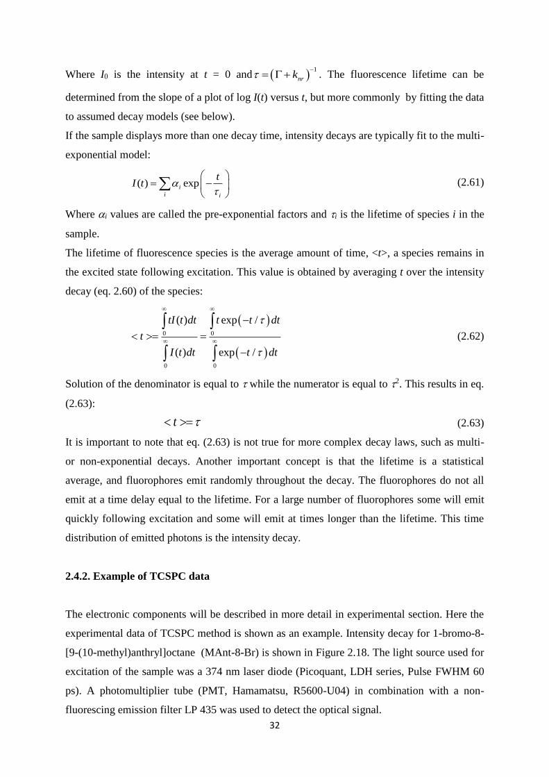
32

Where I0 is the intensity at t = 0 and 1

nrk

. The fluorescence lifetime can be

determined from the slope of a plot of log I(t) versus t, but more commonly by fitting the data

to assumed decay models (see below).

If the sample displays more than one decay time, intensity decays are typically fit to the multi-

exponential model:

( ) expi

i i

tI t

(2.61)

Where i values are called the pre-exponential factors and i is the lifetime of species i in the

sample.

The lifetime of fluorescence species is the average amount of time, <t>, a species remains in

the excited state following excitation. This value is obtained by averaging t over the intensity

decay (eq. 2.60) of the species:

0 0

0 0

( ) exp /

( ) exp /

tI t dt t t dt

t

I t dt t dt

(2.62)

Solution of the denominator is equal to while the numerator is equal to 2. This results in eq.

(2.63):

t (2.63)

It is important to note that eq. (2.63) is not true for more complex decay laws, such as multi-

or non-exponential decays. Another important concept is that the lifetime is a statistical

average, and fluorophores emit randomly throughout the decay. The fluorophores do not all

emit at a time delay equal to the lifetime. For a large number of fluorophores some will emit

quickly following excitation and some will emit at times longer than the lifetime. This time

distribution of emitted photons is the intensity decay.

2.4.2. Example of TCSPC data

The electronic components will be described in more detail in experimental section. Here the

experimental data of TCSPC method is shown as an example. Intensity decay for 1-bromo-8-

[9-(10-methyl)anthryl]octane (MAnt-8-Br) is shown in Figure 2.18. The light source used for

excitation of the sample was a 374 nm laser diode (Picoquant, LDH series, Pulse FWHM 60

ps). A photomultiplier tube (PMT, Hamamatsu, R5600-U04) in combination with a non-

fluorescing emission filter LP 435 was used to detect the optical signal.

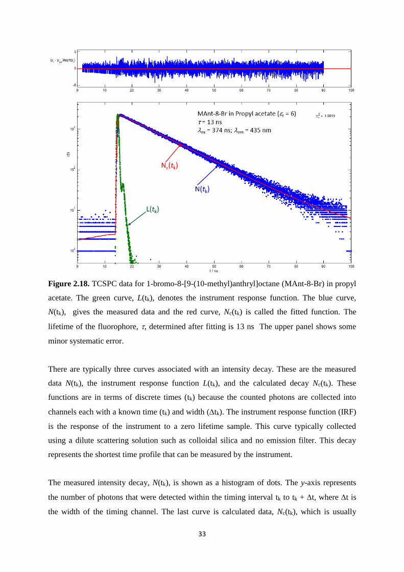
33

Figure 2.18. TCSPC data for 1-bromo-8-[9-(10-methyl)anthryl]octane (MAnt-8-Br) in propyl

acetate. The green curve, L(tk), denotes the instrument response function. The blue curve,

N(tk), gives the measured data and the red curve, Nc(tk) is called the fitted function. The

lifetime of the fluorophore, , determined after fitting is 13 ns The upper panel shows some

minor systematic error.

There are typically three curves associated with an intensity decay. These are the measured

data N(tk), the instrument response function L(tk), and the calculated decay Nc(tk). These

functions are in terms of discrete times (tk) because the counted photons are collected into

channels each with a known time (tk) and width (tk). The instrument response function (IRF)

is the response of the instrument to a zero lifetime sample. This curve typically collected

using a dilute scattering solution such as colloidal silica and no emission filter. This decay

represents the shortest time profile that can be measured by the instrument.

The measured intensity decay, N(tk), is shown as a histogram of dots. The y-axis represents

the number of photons that were detected within the timing interval tk to tk + t, where t is

the width of the timing channel. The last curve is calculated data, Nc(tk), which is usually

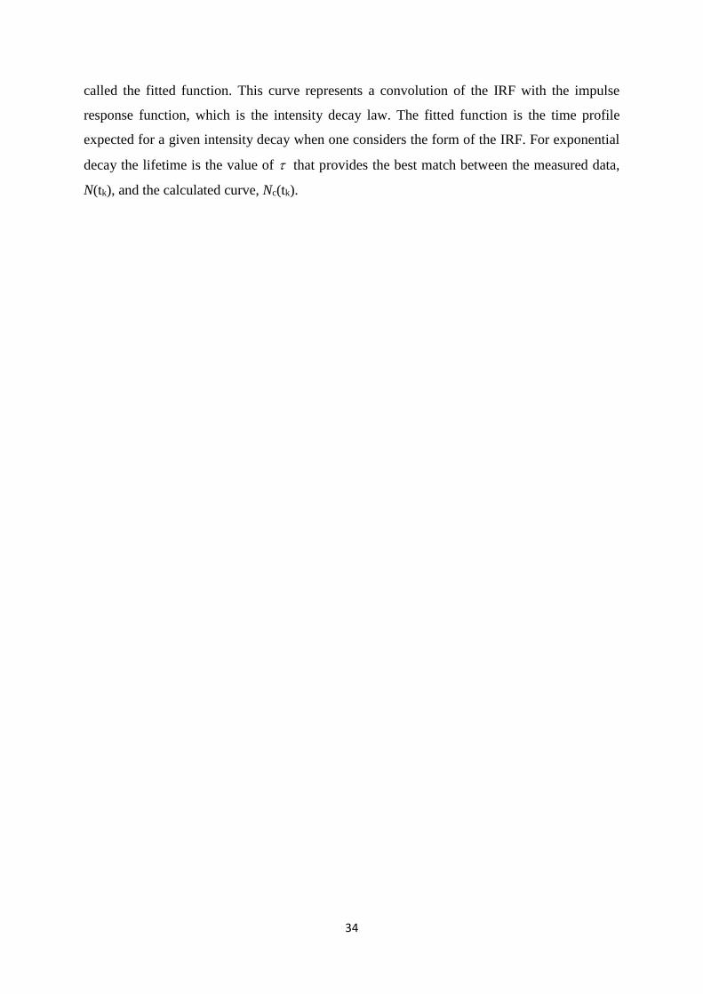
34

called the fitted function. This curve represents a convolution of the IRF with the impulse

response function, which is the intensity decay law. The fitted function is the time profile

expected for a given intensity decay when one considers the form of the IRF. For exponential

decay the lifetime is the value of that provides the best match between the measured data,

N(tk), and the calculated curve, Nc(tk).

35

3. EXPERIMENTAL

3.1. Reactants

In this thesis inter- and intra-acceptor/donor systems were used to investigate electron transfer

driving force and solvent dependences on the mechanism of fluorescence quenching and

magnetic field effects (MFEs) of the exciplexes in inter- and intramolecular photo-induced ET

reactions.

3.1.1. Inter-molecular photo-induced electron transfer systems

3.1.1.1. Acceptors (fluorophores)

9,10-Dimethylanthracene (DMAnt, Aldrich, 99%) was used as received, 9-methylanthracene

(MAnt, Aldrich, 98%) and anthracene (Ant, Aldrich, 99%) were recrystallized from ethanol.

The chemical structures and some parameters of the fluorophores are shown in Figure 3.1 and

Table 3.1.

CH3

CH3

9,10-Dimethylanthracene (DMAnt)

CH3

9-Methylanthracene (MAnt)

Anthracene (Ant)

Figure 3.1. Chemical structures of electron acceptors used in time-resolved magnetic field

effect studies.

3.1.1.2. Donors (quenchers)

N,N-dimethylaniline (DMA, Aldrich, 99.5%) and N,N-diethylaniline (DEA, Aldrich, 99.5%)

were distilled under reduced pressure and subsequently handled under an argon atmosphere.

36

Structures and some parameters of the donors used in the magnetic field studies are depicted

in Figure 3.2 and Table 3.1.

Inter-acceptor/donor pairs used in this thesis provide a change of free energy difference, -G0,

of the photo-induced ET within a range from 0.28 to 0.58 eV.

N

CH3H3C

N

CH2CH3CH3H2C

N,N-Dimethylaniline(DMA)

N,N-Diethylaniline(DEA)

Figure 3.2. Chemical structures of electron donors used in experiments

3.1.2. Intra-molecular photo-induced electron transfer systems

A brief summary of the used chemicals for the synthesis of polymethylene-linked

acceptor/donor systems refers to Table 3.2. The chain-linked 9-methylanthracene (Mant)/N,N-

dimethylaniline (DMA) systems, Mant-(CH2)n-O-(CH2)2-DMA (Mant-n-O-2-DMA), were

synthesized by the following procedure (Scheme 3.1):

9-bromo-10-methylanthracene: This compound was synthesized following the published

procedure [68]. A stirred mixture of 9-methylanthracene (960 mg, 5.0 mmole) and copper (II)

bromide (2.24 g, 5.0 mmole) in chlorobenzene (200 ml) was heated under reflux for 24h. The

reaction mixture was filtered and concentrated in vacuo. The residue was then purified by

chromatography on alumina eluting with n-hexane to obtain 9-bromo-10-methylanthracene

(0.83 g, 60 % yield). Mp: 169-171 0C. See 1H-NMR spectrum in appendix A.2.

1-bromo-10-[9-(10-methyl)anthryl]decane (Mant-10-Br) [45]: 2.5M solution (2.8 ml) of n-

butyllithium in hexane was added dropwise to a solution of 9-bromo-10-methylanthracene (1

g, 3.68 mmole) in dried diethyl ether (20 ml) under argon atmosphere in an ice bath to

maintain the temperature at 0 0C. The mixture was stirred at 0 0C for 4h. After adding 3.4 g

(11.33 mmole) of 1,10-dibromodecane at once, the mixture was stirred for 30 minutes. The

reaction mixture was refluxed for 2h in an oil bath. The resulting mixture was extracted by

37

benzene (325 ml). The benzene layers were combined and washed with water (250 ml).

The separated organic layer was dried over MgSO4 overnight. The solution was concentrated

in vacuo. The residue was absorbed on the Silica gel and run column chromatography eluting

with n-hexane to give Mant-10-Br (0.78 g, 52% yield). Mp: 77-78 0C. The 1H-NMR spectrum

is shown in appendix A.2.

Table 3.1. Physical parameters of the used acceptors and donors [67]: The 0,0-energy E00,

lifetime of acceptors (A), A, and donors (D), D, reduction and oxidation potentials, 𝑬𝟏/𝟐𝒓𝒆𝒅 and

𝑬𝟏/𝟐𝒐𝒙 , respectively. The free energy difference of electron transfer -G0 was calculated at s =

13 in propyl acetate/butyronitrile mixture, using the Rehm-Weller equation with Born

correction assuming an inter-particle distance of 6.5 Å [55] and an ion radius of 3.25 Å.

A E00 /

eV A / ns

𝑬𝟏/𝟐𝒓𝒆𝒅 / V

vs. SCE,

ACNb

𝑬𝟏/𝟐𝒐𝒙 / V

vs. SCE,

ACNb

-G0 (s = 13)

/ eV

DMAnt 3.07 13.0a -1.98 +0.95 0.28

MAnt 3.20 5.8a -1.97 +0.96 0.47

Ant 3.29 5.3a -1.95 +1.16 0.58

D E00

/ eV D / ns

𝑬𝟏/𝟐𝒓𝒆𝒅 / V

vs. SCE,

ACNb

𝑬𝟏/𝟐𝒐𝒙 / V

vs. SCE,

ACNb

DMA - - - +0.81

DEA - - - +0.76

a lifetime measured in acetonitrile (ACN) b acetonitrile (ACN)

38

2-[4-(dimethylamino)phenyl]ethyl 10-[9-(10-methyl)anthryl]decyl ether (Mant-10-O-2-

DMA) [45]: Mant-10-Br (0.65 g, 1.58 mmole ) and 2-[(4-dimethylamino)phenyl]ethanol

(0.56 g, 3.39 mmole) were added to solution of 0.57 g NaH 60% oil suspension in N,N-

dimethylacetamide (15 ml) and the mixture was stirred for 4h in an ice bath at 0 0C. The

resulting mixture was extracted by benzene (315 ml). The benzene layer was washed by cold

water (320 ml) and then dried over MgSO4 overnight. The solvent was removed in vacuo.

The product was isolated by column chromatography on Silica gel with n-hexane and n-

hexane-ethyl acetate (95:5) mixture as eluting solvent systems to obtain Mant-10-O-2-DMA

(0.25 g, 38% yield). Formula: C35H45ON, Mp: 55-56 0C. The 1H, 13C-NMR and mass spectra

are shown in appendix A.2. 1H-NMR (CDCl3, MHz) = 8.6-7.4 ppm (8H, anthracene ring),

7.2-6.7 (4H, benzene ring), 3.7-3.5 (4H, -CH2-O-), 3.45 (2H, -CH2-DMA), 3.1 (3H, CH3-

anthracene), 2.95 (6H, (CH3)2N-), 2.8 (2H, -CH2-anthracene), 2.0-1.2 (16H, chain). MS (EI)

m/z 495.35 (M+, 100).

Other chain-linked acceptor/donor pairs with different chain lengths (Mant-n-O-2-DMA, n =

6, 8, 16) are prepared in the same procedure: Mant-6-O-2-DMA (C31H37ON, Mp: 49-50 0C);

Mant-8-O-2-DMA (C33H41ON, Mp: 71-72 0C); Mant-16-O-2-DMA (C41H57ON, Mp: 53-54

0C). The 1H, 13C-NMR, mass spectra of these compounds are shown in appendix A.2. For

synthesis of Mant-16-O-2-DMA compound, the starting material of 1,16-dibromohexadecane

(1,16-DBHD) is not commercially available. 1,16-DBHD was synthesized by the following

procedure [69]: To a stirred solution of N-bromosuccinimide (2.75 g, 15.45 mmole) in 50 ml

of tetrahydrofuran (THF) at 0 0C, a solution of triphenylphosphine (4.06 g, 14.59 mmole) in

50 ml of THF was added dropwise. After reaching room temperature a solution of

hexadecane-1,16-diol (1.0 g, 3.87 mmole) in 10 ml of THF was also added dropwise. The

mixture is heated at 55 0C for 2.5h. The solvent was evaporated under vacuum. Water was

added to the residue and the solution was extracted with diethyl ether. The organic layer was

washed with water, dried with MgSO4, filtrated and then concentrated in vacuo. Silica gel

chromatography of the resulting solid with n-heptane as eluent gives 1,16-dibromohexadecane

(0.82 g, 55% yield) as a white solid. Mp: 56-57 0C. 1,16-DBHD was used in the next steps.

39

CH3 CH3

Br

CH3

(CH2)n Br

CH3

(CH2)n

O

N

H3C CH3

N

H3C

OH

CH3

CuBr2 Br(CH2)nBr

9-Methylanthracene 9-Bromo-10-methylanthracene Mant-n-Br

Mant-n-O-2-DMA

n = 6, 8, 10, 16

n-BuLi NaH

Scheme 3.1. The synthesis of the polymethylene-linked acceptor/donor systems.

Table 3.2. Chemicals used in the synthetic steps of the polymethylene-linked acceptor/donor

systems. Abbreviations: Mant: 9-methylanthracene, 1,6-DBH: 1,6-dibromohexane, 1,8-DBO:

1,8-dibromooctane, 1,10-DBD: 1,10-dibromodecane, 1,16-HDDO: 1,16-hexadecanediol,

DMAPE: 2-[(4-dimethylamino)phenyl]ethanol. Supplier and purification are indicated.

Chemicals Supplier Purification

Mant Aldrich (99%) as received

1,6-DBH Aldrich (96%) as received

1,8-DBO Aldrich (98%) as received

1,10-DBD Aldrich (98%) as received

1,16-HDDO Aldrich (97%) as received

DMAPE Aldrich (99%) as received

3.2. Solvents

During this work micro-homogeneous solvent mixtures were used. The homogeneity is due to

the difference in dielectric constants and the mutual miscibility of the two components in

40

binary solvent mixtures [30, 31]. The three macroscopic solvent properties of main interest in

the presented studies are: the viscosity, , the refractive index, n, and the static dielectric

constant, s. All solvents used, their macroscopic properties of interest and their purification

are summarized in Table 3.3. Series of mixture of propyl acetate (PA) and butyronitrile (BN)

with varying dielectric constant, s, in a range from 6 to 24.7. The dielectric constant was

calculated from: 𝜀(𝑤1) = 𝑤1𝜀1 + (1 − 𝑤1)𝜀2 with 𝑤𝑖 and 𝜀𝑖 denoting the weight fraction and

dielectric constant of component i [30, 31, 36]. In these mixtures (Table 3.4), the viscosity (

= 0.58 cP), and thus, the diffusion coefficients are nearly constant (maximum variation of

1.2%). The refractive index (n = 1.383) is likewise almost invariant with solvent composition

[30, 36]. The Pekar factor (1/n2 – 1/s) of PA/BN mixtures, which governs the outer-sphere

electron transfer reorganization energy and, thus the rate of the ET processes, varies by only

5% in the studied s-range [1, 3]. Propionitrile (EtCN) and acetonitrile (ACN) were used to

extend the solvent polarity range in intra-molecular photo-induced ET reactions.

Table 3.3. Macroscopic solvent properties are given at 25 0C: density (), dielectric constant

(s), dynamic viscosity (), refractive index (n). Additionally the solvent supplier and the

purification methods are given. Abbreviations: PA: propyl acetate, BN: butyronitrile. ACN:

acetonitrile, EtCN: propionitrile. All solvent properties were taken from reference [70].

Solvent /

g mL-1 s

/

cP n Supplier Purification

PA 0.888 6.0 0.58 1.383 Aldrich

(99.5%) distilled

BN 0.794 24.6 0.58 1.383 Fluka (99%) distilled

ACN 0.782 36.0 0.34 1.341 Aldrich

(99.8%) distilled

EtCN 0.776 28.3 0.39 1.363 Aldrich

(99.5%) distilled

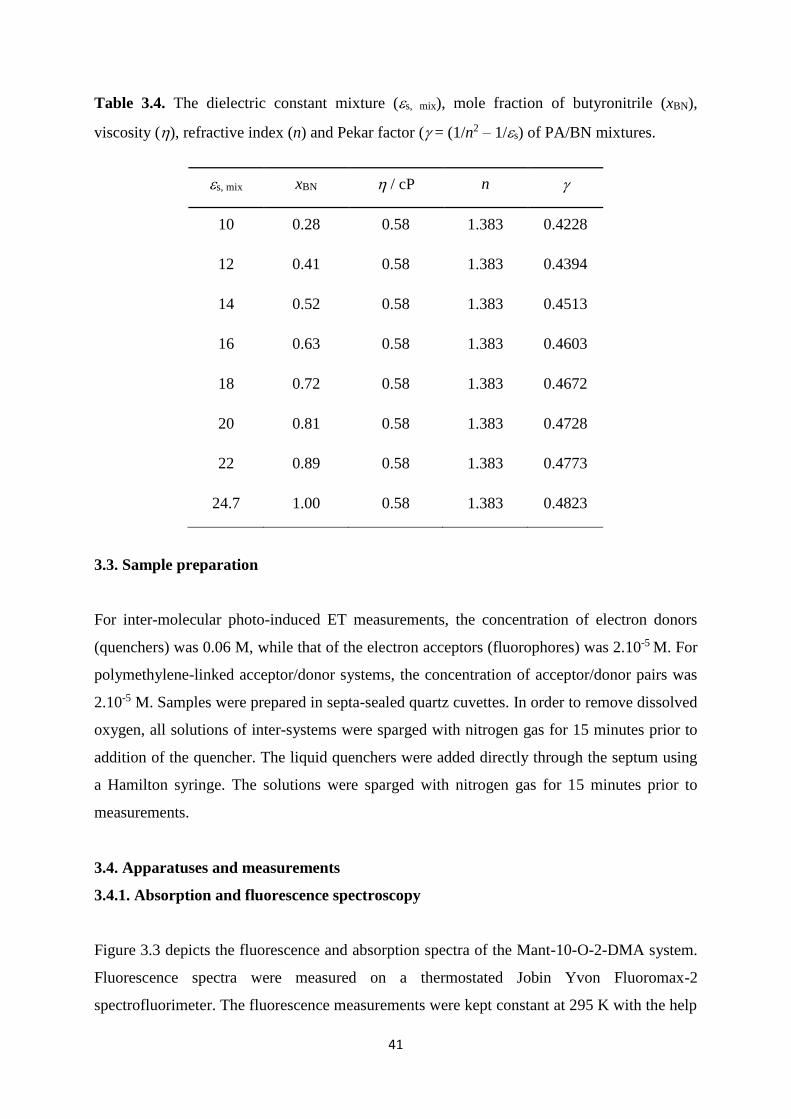
41

Table 3.4. The dielectric constant mixture (s, mix), mole fraction of butyronitrile (xBN),

viscosity (), refractive index (n) and Pekar factor ( = (1/n2 – 1/s) of PA/BN mixtures.

s, mix xBN / cP n

10 0.28 0.58 1.383 0.4228

12 0.41 0.58 1.383 0.4394

14 0.52 0.58 1.383 0.4513

16 0.63 0.58 1.383 0.4603

18 0.72 0.58 1.383 0.4672

20 0.81 0.58 1.383 0.4728

22 0.89 0.58 1.383 0.4773

24.7 1.00 0.58 1.383 0.4823

3.3. Sample preparation

For inter-molecular photo-induced ET measurements, the concentration of electron donors

(quenchers) was 0.06 M, while that of the electron acceptors (fluorophores) was 2.10-5 M. For

polymethylene-linked acceptor/donor systems, the concentration of acceptor/donor pairs was

2.10-5 M. Samples were prepared in septa-sealed quartz cuvettes. In order to remove dissolved

oxygen, all solutions of inter-systems were sparged with nitrogen gas for 15 minutes prior to

addition of the quencher. The liquid quenchers were added directly through the septum using

a Hamilton syringe. The solutions were sparged with nitrogen gas for 15 minutes prior to

measurements.

3.4. Apparatuses and measurements

3.4.1. Absorption and fluorescence spectroscopy

Figure 3.3 depicts the fluorescence and absorption spectra of the Mant-10-O-2-DMA system.

Fluorescence spectra were measured on a thermostated Jobin Yvon Fluoromax-2

spectrofluorimeter. The fluorescence measurements were kept constant at 295 K with the help

42

of a Haake-F3 thermostat. A theoretical model has to be employed to extract the exciplex

emission [35], e.g, a sum of vibronic transitions with Gaussian band shape can be assumed

[71]. Absorption spectra were recorded on a Shimadzu UV-3101-PC UV-VIS-NIR

spectrometer. All absorption and fluorescence spectra of inter-systems and intra-systems

Mant-n-O-2-DMA (n = 6, 8, 16) compounds are shown in appendix A.3.

3.4.2. Steady-state magnetic field effect measurements

Magnetic field effects (MFEs) on exciplexes from steady-state measurements were recorded

using a thermostated cell (295 K) coupled to a Jobin Yvon FluoroMax2 fluorescence

spectrometer via light guides. The magnetic field in the sample compartment was measured

using a F. W. Bell Model-9200 gaussmeter. A saturating magnetic field of 62 mT was

employed. The earth magnetic field and stray fields were not compensated, i.e., the ‘‘zero

field’’ reading corresponds to approximately 0.08 mT. The MFEs on systems were obtained

by detecting the fluorescence intensity at 550 nm (Figure 3.3) for 60 s, using a spectrometer

time constant of 1 s. For each sample, fluorescence intensities were acquired alternating three

times between zero and saturating magnetic field. In general, the excitation slit width was 2

nm and the emission slit width 6 nm. All fluorescence signals have been background

corrected. The three repetitions were analysed independently and the experimental errors were

obtained according to the method described in reference [54]. Time scans at the emission

wavelength of the exciplex were used to evaluate the absolute MFE on the exciplex, SS,

given by:

0

0 0 0

( , ) ( , )

( , ) ( ( , ) ( )) / ( )

em sat emSS

Fem em em c em

I B I B

I B I B BG I I BG

(3.1)

Here, ( , )em satI B and 0( , )emI B are the mean intensities at em in a saturated magnetic field,

Bsat, and in the absent magnetic field, B0. 0( , )F emI B is the residual emission of the locally-

excited fluorophore at em in the absence of quencher. Ic and I0 are the fluorescence intensities

in the presence and absence of quencher. Ic/I0 is the relative intensity of the prompt emission

of the fluorophore in the presence of the quencher as obtained from the fluorescence spectra

decomposition and ( )emBG is the mean background intensity.

43

Figure 3.3. Absorption and fluorescence spectra of Mant-10-O-2-DMA in a mixture of propyl

acetate/butyronitrile at s = 12. The emissions of the locally excited acceptor and the exciplex

are shaded in blue and red, respectively.

3.4.3. Time-resolved magnetic field effect measurements

Figure 3.4 shows the time-resolved magnetic field effect (TR-MFE) of the exciplex of Mant-

16-O-2-DMA system. The TR-MFE spectra of other systems are given in appendix A.4. All

TR-MFE measurements have been performed at 295 K. The time-resolved emission data of

the exciplex were collected by the Time-Correlated Single Photon-Counting (TCSPC) method

with the sample immersed in the magnetic field of a Bruker B-E10B8 electromagnet. The

electromagnet was set to B0 = 0 mT or 62 mT, the magnetic flux density being measured by a

Hall probe placed next to the cuvette half-way between the pole pieces. The sample holder

was fabricated from and thermostated by circulating. The acceptor moieties were excited at

374 nm using a picosecond diode laser (Picoquant, LDH-P-C-405, FWHM 60 ps). A 550 nm

long-pass filter was placed in front of the detector to extract the exciplex emission.

The used setup is depicted in Figure 3.5. The light source is driven by an external pulse

generator (Stanford Research Systems, INC, Model DG-535) with a repetition rate of 0.8

MHz. The experiment is commenced by the excitation pulse that excites the sample and

triggers the time-to-amplitude converter. This signal is passed through a constant function

discriminator (CFD), which accurately measures the arrival time of the pulse. This signal is

passed to a time-to-amplitude converter (TAC). The arrival time of the signal is accurately

determined using a second CFD. In the front of the light source, an UV-passing filter [4]

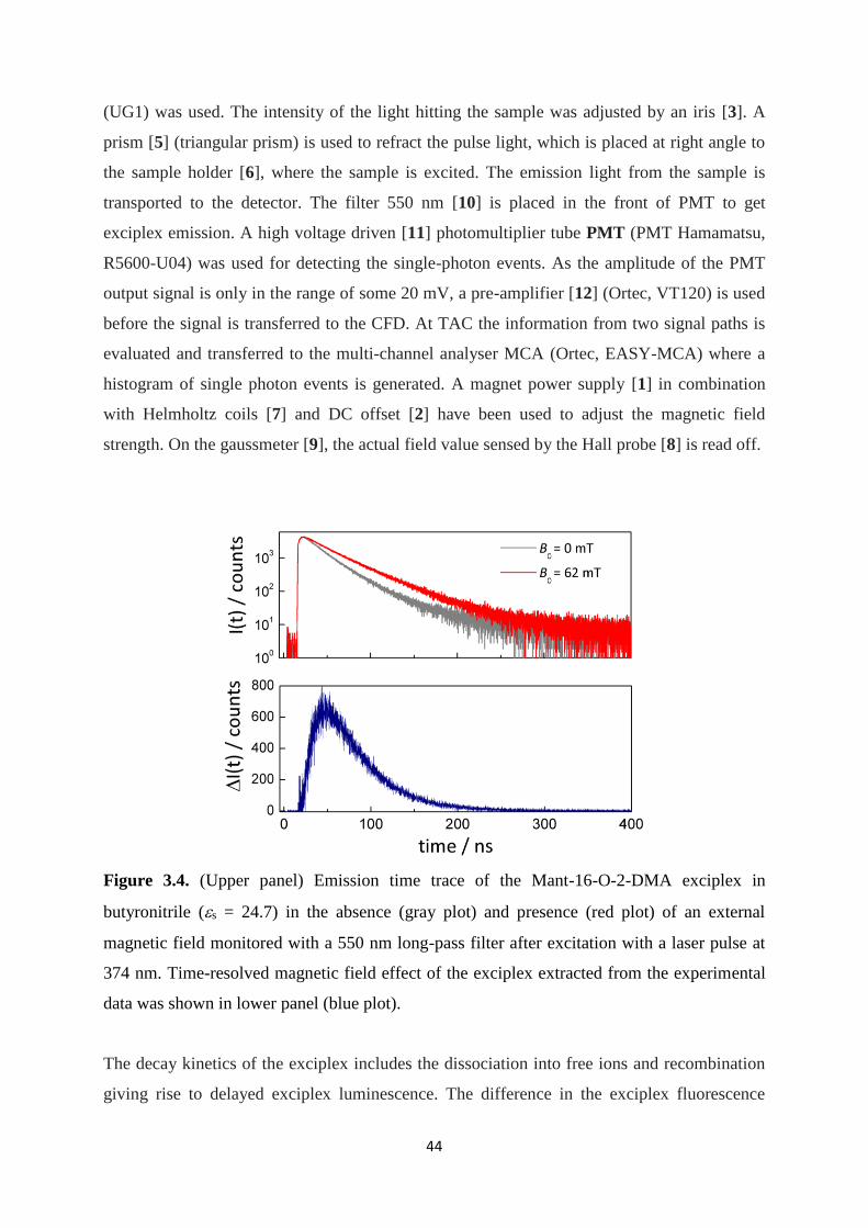
44

(UG1) was used. The intensity of the light hitting the sample was adjusted by an iris [3]. A

prism [5] (triangular prism) is used to refract the pulse light, which is placed at right angle to

the sample holder [6], where the sample is excited. The emission light from the sample is

transported to the detector. The filter 550 nm [10] is placed in the front of PMT to get

exciplex emission. A high voltage driven [11] photomultiplier tube PMT (PMT Hamamatsu,

R5600-U04) was used for detecting the single-photon events. As the amplitude of the PMT

output signal is only in the range of some 20 mV, a pre-amplifier [12] (Ortec, VT120) is used

before the signal is transferred to the CFD. At TAC the information from two signal paths is

evaluated and transferred to the multi-channel analyser MCA (Ortec, EASY-MCA) where a

histogram of single photon events is generated. A magnet power supply [1] in combination

with Helmholtz coils [7] and DC offset [2] have been used to adjust the magnetic field

strength. On the gaussmeter [9], the actual field value sensed by the Hall probe [8] is read off.

Figure 3.4. (Upper panel) Emission time trace of the Mant-16-O-2-DMA exciplex in

butyronitrile (s = 24.7) in the absence (gray plot) and presence (red plot) of an external

magnetic field monitored with a 550 nm long-pass filter after excitation with a laser pulse at

374 nm. Time-resolved magnetic field effect of the exciplex extracted from the experimental

data was shown in lower panel (blue plot).

The decay kinetics of the exciplex includes the dissociation into free ions and recombination

giving rise to delayed exciplex luminescence. The difference in the exciplex fluorescence

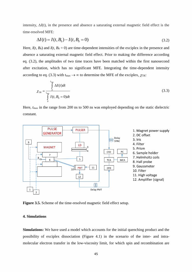
45

intensity, I(t), in the presence and absence a saturating external magnetic field effect is the

time-resolved MFE:

0 0( ) ( , ) ( , 0)I t I t B I t B (3.2)

Here, I(t, B0) and I(t, B0 = 0) are time-dependent intensities of the exciplex in the presence and

absence a saturating external magnetic field effect. Prior to making the difference according

eq. (3.2), the amplitudes of two time traces have been matched within the first nanosecond

after excitation, which has no significant MFE. Integrating the time-dependent intensity

according to eq. (3.3) with tmax to determine the MFE of the exciplex, TR:

max

max

0

0

0

( )

( , 0)

t

TR t

I t dt

I t B dt

(3.3)

Here, tmax in the range from 200 ns to 500 ns was employed depending on the static dielectric

constant.

Figure 3.5. Scheme of the time-resolved magnetic field effect setup.

4. Simulations

Simulations: We have used a model which accounts for the initial quenching product and the

possibility of exciplex dissociation (Figure 4.1) in the scenario of the inter- and intra-

molecular electron transfer in the low-viscosity limit, for which spin and recombination are

46

treated independently [36]. According to this model, the probability that the system is

observed in the exciplex state, E, is given as:

𝜌𝐸(𝑡, 𝐵0) = 𝜙𝐸 + 𝜙𝐼𝑅(𝑡|𝑟𝐼 , 𝐵0) + 𝑘𝑑 ∫ 𝜌𝐸(𝜏)𝑅(𝑡 − 𝜏|𝑟𝐸 , 𝐵0)𝑑𝜏 − (𝑘𝑑 + 𝜏𝐸−1𝑡

0) ∫ 𝜌𝐸(𝜏)𝑑𝜏

𝑡

0

(4.1)

Here, 𝑟𝐼 is the distance where the loose ion pair is formed by (distant) electron transfer, 𝑟𝐸 the

contact distance of donor and acceptor from which the exciplex is eventually formed,

𝑅(𝑡|𝑟𝐼 , 𝐵0) refers to the probability that the RIP formed at t = 0 at distance rI has recombined

until t, and 𝑘𝑑 is the exciplex dissociation rate. The first term in equation (4.1), E = 1 - I, is

the probability that the exciplex is formed initially (path 1A in Figure 2.16), the second term

denotes the probability that the RIP is formed initially and recombines forming the exciplex

until t, the third term gives the probability that the exciplex dissociates with the probability

𝑘𝑑𝜌𝐸(𝜏)𝑑𝑡 at time and is reformed until t, and the last term refers to the depopulation by

dissociation and radiative/non-radiative decay of the exciplex. The exciplex lifetime, E,

shown in Figure 5.9, has been extracted from the initial fluorescence decay. 𝑅(𝑡|𝑟𝐼 , 𝐵0)

depends on the singlet-probability of the radical pair and recombination function, for which a

radiative boundary condition with recombination rate ka was chosen [36].

Figure 4.1: The graphic visualization of the exciplex kinetics of inter-systems (left panel) and

Mant-n-O-2-DMA systems (right panel): I gives the probability of the initial singlet radical

ion pair (SRIP) formation while E = 1-I denotes the probability of the initial exciplex

formation. The exciplex dissociates into the singlet radical ion pair with the rate constant, kd,

the SRIP associates into the exciplex with the rate constant, ka and the radiative/non-radiative

exciplex decay to the ground-state (GS) with the rate constant, 𝜏𝐸−1. LE refers to the locally-

excited acceptor.

47

The association constant, KA = ka/kd (ka is the rate of RIP association into exciplex), has been

determined (besides I and d) to reproduce the experimental MFE in the least-squares sense.

The kd values so obtained are plotted in Figures 5.10 as a function of dielectric constant.

Simulation parameters: The time evolution of the MFE depends on the following

parameters:

a) Diffusive motion

D: diffusion coefficient (estimated from the Stokes-Einstein relation assuming a

hydrodynamic radius of 3.25 Å)

rE: contact distance of donor and acceptor (6.5 Å)

rc: Onsager radius (𝑟𝑐 =𝑒0

2

4𝜋𝜀0𝜀𝑟𝑘𝐵𝑇) (calculated from the solvent dielectric constant)

Hydrodynamic hindrance (the Deutch-Felderhof model has been used [20])

b) Exciplex

E: exciplex lifetime (determined from a bi-exponential fit to the initial fluorescence

decay).

d = kdE: dissociation quantum yield of the exciplex

c) Radical ion pair (RIP)

Spin evolution (calculated as described in [36] using the hyperfine coupling constants

reported below)

R: radical ion pair lifetime (200 ns)

rI: distance where ions are generated by distant ET (7 Å was used on account of the

fact that the ET is in the Marcus normal region)

I: initial probability of the RIP state

ka = KAkd: rate of RIP association into exciplex

Most of listed parameters are either known, or can be determined in independent

experimental measurements and kept constant during simulations. E can be

determined experimentally, and d values obtained are close to those calculated from

the dependence of E on the solvent polarity.

Tables 4.1-4.5 list the hyperfine coupling constants that have been used to calculate the spin

evolution of the RIP.

48

Table 4.1. Used hyperfine coupling constants, 𝑎−𝐻, for anthracene-. taken from [72-73].

Value / mT -0.556 -0.274 -0.157

Type 2H 4H 4H

Position (9, 10) (1, 4, 5, 8) (2, 3, 6, 7)

Table 4.2. Used hyperfine coupling constants, |𝑎−𝐻|, for 9-methylanthracene-. taken from [72].

Value/ mT 0.427 0.516 0.294 0.139 0.173 0.277

Type 3H 1H 2H 2H 2H 2H

Position (-CH3) (10) (1, 8) (2, 7) (3, 6) (4, 5)

Table 4. 3. Used hyperfine coupling constants, 𝑎−𝐻, for 9,10-dimethylanthracene-. taken from

[72].

Value / mT 0.388 0.290 -0.152

Type 6H 4H 4H

Position (-2CH3) (1, 4, 5, 8) (2, 3, 6, 7)

Table 4.4. Used hyperfine coupling constants, 𝑎+𝐻, for the radical cation of N,N-

diethylaninline+.. No experimental values are available, the values below have been calculated

using DFT (UB3LYB/EPRII).

Value / mT 0.9222 -0.7910 0.1922 -0.5294 0.7315 -0.0018

Type 1N 1H 2H 2H 4H 6H

Position (N) (4) (3, 5) (2, 6) (>2CH2) (-2CH3)

Table 4.5. Used hyperfine coupling constants, 𝑎+𝐻, for N,N-dimethylaniline+.. No

experimental values are available, the values below have been calculated using DFT

(UB3LYB/EPRII).

Value / mT 0.833 -0,428 0.0868 -0.722 1.30

Type 1N 2H 2H 1H 6H

Position (N) (2, 6) (3, 5) (4) (-2CH3)

49

Calculations of the Singlet Probability / and the Recombination Function:

The singlet probability 0( , )S t B is given by:

0 0ˆ ˆ( , ) ( , )S St B Tr P t B

(4.2)

Where ˆSP refers to the singlet projection operator, Tr is the trace operator, and the time

behavior of the spin density matrix 0ˆ( , )t B is obtained from the Liouville-von-Neumann

equation:

ˆ ˆˆ ˆˆ ˆ, ex

di H K

dt

(4.3)

With the initial density matrix given by:

ˆˆ( 0)

ˆ( )

SPt

Tr

(4.4)

In the low-viscosity approximation, the exchange interaction can be neglected, thus, the

Hamiltonian H for a single radical i only contains contributions from the Zeeman interaction

of the electron spins and the hyperfine interactions according to:

,ˆ ˆˆ ˆ

i i B i z ij i ij

j

H g BS a S I (4.5)

Since only moderate magnetic fields are employed, it is furthermore assumed that g1 = g2 =

2.0023. The influence of the exchange operator ˆ

exK accounting for degenerate electron

exchange is then calculated from:

ˆ1 1ˆˆ ˆ ˆ( )ex n

ex

K TrN

(4.6)

In this work, the spin correlation tensor approach was used to calculate the singlet probability

(Figure 4.2). This approach implies a reformulation of Equations (4.3, 4.4, 4.6) which allows

a more efficient numerical treatment of the problem in Hilbert space. Details can be found in

references [28, 29, 74]. For the pseudo first-order self-exchange rate constant, kex = 1/ex, a

value of ex = 8 ns was used in all simulations.

50

Figure 4.2. Calculated singlet probability as a function of time for anthracene/N,N-

diethylaniline at zero field and high field limit. The solid lines denote pS(t) when the electron

self-exchange taken into account with ex = 8 ns whereas the dash lines show pS(t) with

neglecting the electron self-exchange.

In this work a diffusion Green’s function approach [21, 75] has been used to calculate the

singlet yields from:

0 0

0

( , | ) ( , ) ( | )exp

t

I S I

R

tR t B r t B f t r dt

(4.7)

With ( | )If t r denoting the recombination flux, and R the radical pair lifetime. The

recombination flux is the defined as:

( | ) ( , | )I a E If t r k n r t r (4.8)

With the time-dependence of ( , )n r t given by:

2

2

( , ) 1( ) exp( ) exp( ) ( , )

c c

n r t r rD r r n r t

t r r r r r

(4.9)

Where 2

0

04c

s B

er

k T denotes the Onsager radius. The initial condition (for instantaneous

RIP generation) is taken to be:

2( , 0) ( ) / 4In r t r r r (4.10)

and the system obeys the radiation boundary condition:

2 2|

4 ( ) E

c ar r

E E

r knn n

r r r D r

(4.11)

51

5. RESULTS AND DISCUSSION

5.1. Magnetic field effect dependence on the static dielectric constant and chain length

Figure 5.1 depicts the magnetic field effects (MFEs) of the exciplexes of inter- and intra-

donor/acceptor systems in PA/BN mixtures, propionitrile (EtCN) and acetonitrile (ACN). The

MFEs were determined from the time-resolved MFE data, TR, by integration according to eq.

(3.3) in comparison to SS determined from steady-state measurements according to eq. (3.1).

Within the experimental error, the two sets of MFE agree, suggesting that all processes

leading to the MFE under the experimental conditions occur on the time window (< 500 ns,

see below). The agreement indicates that the bulk processes, e.g., reencounters of uncorrelated

ions and processes involving fluorophore triplet do not significantly contribute to the MFE

[76]. In fact, the experimental conditions have been chosen under low light intensities and low

fluorophore concentrations to minimize these effects.

MFEs of the exciplexes are functions of the static dielectric constant, s, of the binary solvent

mixtures. For inter-systems, there is no MFE for s < 7. For s > 7 MFEs increase sharply and

obtain the maximum value at s = 18, followed by a monotonous decrease for s > 18. For

intra-systems (Mant-n-O-2-DMA), the onset of the MFE attains at s > 10 and the maximum

MFE obtains at s = 24.7 (neat butyronitrile), followed by a decrease with increasing solvent

polarity. MFEs of the exciplexes are proportional to the intersystem crossing (ISC) rate (S-T

conversion) in the radical ion pairs (RIP) which produced in photo-induced electron transfer

reaction. The spin evolution can only take place if component radicals in RIP diffusively

separate until the exchange interaction between unpaired electrons is negligible to allow a

hyperfine coupling-induced (HFC) intersystem crossing.

The solvent polarity and viscosity can affect the separation distance of the two radicals. The

interaction between solvent molecules (polar components) and exciplexes, RIPs can be

simplified as dipole-dipole interactions [77-78]. At low values of s, the both radicals in RIP

cannot diffuse to the extent of S-T degeneracy, thus ISC is unfavourable and MFE is zero. In

contrast, at high s values, the radical separation is sufficient, but the reencounter probability

is not effective due to the prevention from the polar components (BN) in solvent mixtures.

52

This results in a decrease in the MFEs. At moderate polarity, there is a good compromise

between radical separation and reencounter and the MFE thus is at maximum.

(a) DMAnt/DMA (b) MAnt/DEA

(c) Ant/DEA (d) Mant-8-O-2-DMA

(e) Mant-10-O-2-DMA (f) Mant-16-O-2-DMA

Figure 5.1. The magnetic field effects on inter-system (a-c) and Mant-n-O-2-DMA exciplexes

(d-f) determined from TR-MFE using eq. (3.3) (filled circle with error bars) and from steady-

state measurements using eq (3.1) (open circles with error bars) in propyl acetate/butyronitrile

mixtures by varying the dielectric constant, s. For intra-acceptor/donor systems, pure

propionitrile (EtCN) and acetonitrile (ACN) are used to extend the range of solvent polarity.

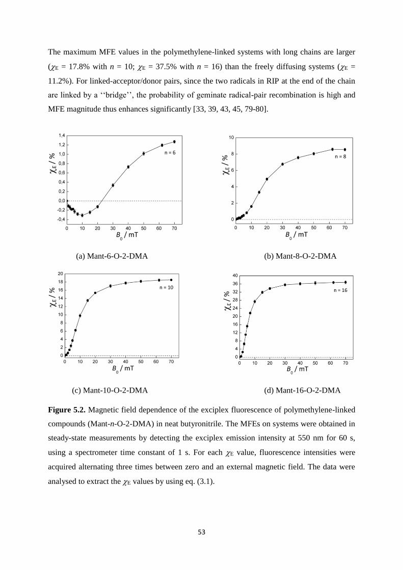
53

The maximum MFE values in the polymethylene-linked systems with long chains are larger

(E = 17.8% with n = 10; E = 37.5% with n = 16) than the freely diffusing systems (E =

11.2%). For linked-acceptor/donor pairs, since the two radicals in RIP at the end of the chain

are linked by a ‘‘bridge’’, the probability of geminate radical-pair recombination is high and

MFE magnitude thus enhances significantly [33, 39, 43, 45, 79-80].

(a) Mant-6-O-2-DMA (b) Mant-8-O-2-DMA

(c) Mant-10-O-2-DMA (d) Mant-16-O-2-DMA

Figure 5.2. Magnetic field dependence of the exciplex fluorescence of polymethylene-linked

compounds (Mant-n-O-2-DMA) in neat butyronitrile. The MFEs on systems were obtained in

steady-state measurements by detecting the exciplex emission intensity at 550 nm for 60 s,

using a spectrometer time constant of 1 s. For each E value, fluorescence intensities were

acquired alternating three times between zero and an external magnetic field. The data were

analysed to extract the E values by using eq. (3.1).

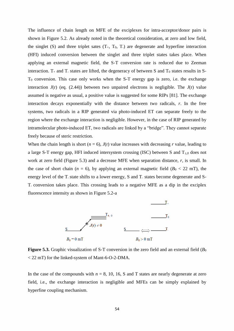
54

The influence of chain length on MFE of the exciplexes for intra-acceptor/donor pairs is

shown in Figure 5.2. As already noted in the theoretical consideration, at zero and low field,

the singlet (S) and three triplet sates (T+, T0, T-) are degenerate and hyperfine interaction

(HFI) induced conversion between the singlet and three triplet states takes place. When

applying an external magnetic field, the S-T conversion rate is reduced due to Zeeman

interaction. T+ and T- states are lifted, the degeneracy of between S and T0 states results in S-

T0 conversion. This case only works when the S-T energy gap is zero, i.e. the exchange

interaction J(r) (eq. (2.44)) between two unpaired electrons is negligible. The J(r) value

assumed is negative as usual, a positive value is suggested for some RIPs [81]. The exchange

interaction decays exponentially with the distance between two radicals, r. In the free

systems, two radicals in a RIP generated via photo-induced ET can separate freely to the

region where the exchange interaction is negligible. However, in the case of RIP generated by

intramolecular photo-induced ET, two radicals are linked by a “bridge”. They cannot separate

freely because of steric restriction.

When the chain length is short (n = 6), J(r) value increases with decreasing r value, leading to

a large S-T energy gap, HFI induced intersystem crossing (ISC) between S and T±,0 does not

work at zero field (Figure 5.3) and a decrease MFE when separation distance, r, is small. In

the case of short chain (n = 6), by applying an external magnetic field (B0 < 22 mT), the

energy level of the T- state shifts to a lower energy, S and T- states become degenerate and S-

T- conversion takes place. This crossing leads to a negative MFE as a dip in the exciplex

fluorescence intensity as shown in Figure 5.2-a

Figure 5.3. Graphic visualization of S-T conversion in the zero field and an external field (B0

< 22 mT) for the linked-system of Mant-6-O-2-DMA.

In the case of the compounds with n = 8, 10, 16, S and T states are nearly degenerate at zero

field, i.e., the exchange interaction is negligible and MFEs can be simply explained by

hyperfine coupling mechanism.

55

The B1/2 value, the magnetic field strength at which the delayed exciplex fluorescence reaches

half its saturation value compared to zero field, is calculated by using the hyperfine-coupling

constants (Ai) of two radicals forming the RIP and can be estimated by eq. (5.1) [82]:

2 2

1 21/2

1 2

2( )A AB

A A

(5.1)

With 2 ( 1)i ik ik ik

k

A a I I where ika and

ikI are the individual isotropic hyperfine coupling

constants and nuclear spin quantum numbers of the radical i, respectively.

In the unlinked pair composed of 9,10-dimethylanthracene and N,N-dimethylaniline, the B1/2

value is 5.32 mT, determined from magnetic field effect on reaction yield (MARY)

experiments and closely matches the theoretical value, 5.27 mT, determined from eq. (5.1)

[30-31]. In the linked systems of Mant-n-O-2-DMA, the B1/2 values, determined from the

plots of the magnetic field dependence of the exciplex luminescence (Figure 5.2), are 18 mT

(n = 8), 9.5 mT (n = 10) and 5.6 mT (n = 16). The larger B1/2 values obtained from the

intramolecular radical pairs can be explained by the effect of the spin exchange interaction

[83]. This effect can suppress the S-T conversion, this effect is reflected in the intra-systems

with shorter length. Since the biradicals are linked by a chain, radical pair dissociation into

free ions does not take place. There is a time-dependent J(r), i.e., the molecular motion is

modulating the exchange interaction. As a consequence the S-T coherences are decaying

faster and this gives rise to the larger B1/2 values.

5.2. Magnetic field effects on the locally excited fluorophore in intra-molecular photo-

induced electron transfer reactions

Figure 5.4 depicts the MFEs on the fluorophore (acceptor) moieties and the exciplex

determined by wavelength-resolved MFE measurements of the Mant-n-O-2-DMA (n = 8, 10,

16) in butyronitrile. Energetic factors, in particular, the free energy gap of the exciplex and

the fluorophore (Figure 2.16), determines the probability of exciplex-fluorophore

reversibility. MFEs on the locally excited (LE) fluorophores have been exhibited to be

significant for the systems characterised by a free energy difference up to approximately -0.35

eV [34-35]. Here, it is assumed that the free energy of charge separation of the fluorophore

and exciplex of intra-systems is the same with the one of the free system (DMAnt/DMA). The

56

free energy difference approximated of the linked-systems is -0.34 eV in butyronitrile [34].

Thus, MFEs on the LE fluorophore are expected.

Wavelength-resolved scans in the absence and presence of a saturating external magnetic field

were taken in turn of five scans under field-off (B0 = 0 mT) and field-on (B0 = 62 mT)

conditions in each case. All acceptor moieties were excited at 378 nm. The magnitude of MFE

of the LE fluorophores and exciplexes was evaluated as = I(B0 = 62 mT)/I(B0 = 0 mT) – 1.

All data have been background corrected.

(a) Mant-8-O-2-DMA (b) Mant-10-O-2-DMA

(c) Mant-16-O-2-DMA

Figure 5.4. Wavelength-resolved magnetic field effects of the Mant-n-O-2-DMA (n = 8, 10,

16) systems in butyronitrile. F and E denote the magnetic field effects on the locally-excited

fluorophore and the exciplex, respectively.

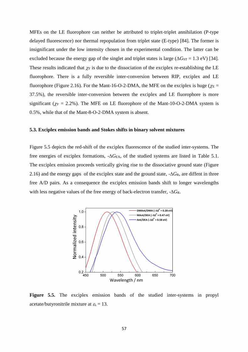
57

MFEs on the LE fluorophore can neither be attributed to triplet-triplet annihilation (P-type

delayed fluorescence) nor thermal repopulation from triplet state (E-type) [84]. The former is

insignificant under the low intensity chosen in the experimental condition. The latter can be

excluded because the energy gap of the singlet and triplet states is large (GST = 1.3 eV) [34].

These results indicated that F is due to the dissociation of the exciplex re-establishing the LE

fluorophore. There is a fully reversible inter-conversion between RIP, exciplex and LE

fluorophore (Figure 2.16). For the Mant-16-O-2-DMA, the MFE on the exciplex is huge (E =

37.5%), the reversible inter-conversion between the exciplex and LE fluorophore is more

significant (F = 2.2%). The MFE on LE fluorophore of the Mant-10-O-2-DMA system is

0.5%, while that of the Mant-8-O-2-DMA system is absent.

5.3. Exciplex emission bands and Stokes shifts in binary solvent mixtures

Figure 5.5 depicts the red-shift of the exciplex fluorescence of the studied inter-systems. The

free energies of exciplex formations, -GEX, of the studied systems are listed in Table 5.1.

The exciplex emission proceeds vertically giving rise to the dissociative ground state (Figure

2.16) and the energy gaps of the exciplex state and the ground state, -GR, are diffent in three

free A/D pairs. As a consequence the exciplex emission bands shift to longer wavelengths

with less negative values of the free energy of back-electron transfer, -GR.

Figure 5.5. The exciplex emission bands of the studied inter-systems in propyl

acetate/butyronitrile mixture at s = 13.

58

Table 5.1. Some parameters of the studied A/D pairs at s = 13 in propyl acetate/butyronitrile

mixture. E00 is the 0-0 transition energy of acceptor; -GEx refers to the free energy of

exciplex formation; -GR gives the free energy of back-electron transfer; max denotes the

maximum wavelength of the exciplex emission band.

A/D E00 / eV -GEx (s = 13)

/ eV

-GR (s = 13)

/ eV max / nm

DMAnt/DMA 3.07 0.28 2.79 512

MAnt/DEA 3.20 0.47 2.73 528

Ant/DEA 3.29 0.58 2.71 540

Figure 5.6 shows the wavelength shifts of the exciplex fluorescence bands with different

solvent dielectric constant, s, in PA/BN mixtures. There are Stokes shifts of the exciplex

spectra with increasing the solvent polarity. This effect is based on the solvent relaxation

properties in the excited complexes (exciplexes) [66]. In particular, the preferential solvation

of polar component in binary solvent is involved in this effect [85-86]. After photo-excitation,

an excited acceptor diffusively approaches an electron donor, under a well-defined relative

orientation [5-9], an excited-state charge-transfer complex (exciplex) is formed. The exciplex

shows a dipole moment. Polar solvent molecules in binary mixture can diffuse from the bulk

to the surface of the dipolar solute molecules (exciplexes) to generate a solvent shell or polar

clusters surrounding exciplex due to dipole-dipole interaction [77-78]. The concentration of

polar components (BN) in solvent shell increases with increasing their mole fractions. The

enrichment of polar solvent molecules in solvent shell gives rise to a difference between the

effective dielectric constant around exciplex and the bulk dielectric constant. This effect is

reflected in the red shifts of exciplex emission bands with increasing the mole fraction of

polar components in binary mixtures.

In energetic aspect, this effect is also predicted from the solvent dielectric constant

dependence of the driving force of exciplex formation, GEx. The GEx values of chain-linked

acceptor/donor pairs are calculated as the calculation was applied for the free acceptor/donor

pair of DMAnt/DMA system. The -GEx ranges from 0.30 eV for s = 6 to 0.34 eV for s =

59

24.7 [34]. The driving forces of exciplex formation become slightly more negative with

increasing s values, i.e. the energy gap between the locally excited fluorophore

(acceptor)/quencher (donor) pair and the exciplex (see Figure 2.16) is larger. As a

consequence the maximum peak position of the exciplex emission to ground state is shifted to

the longer wavelengths.

(a) MAnt/DEA (b) Ant/DEA

(c) Mant-10-O-2-DMA (d) Mant-16-O-2-DMA

Figure 5.6. Exciplex fluorescence spectra of inter-systems (a-b) and Mant-n-O-2-DMA

systems (c-d) in neat propyl acetate (PA), butyronitrile (BN) and mixtures of propyl

acetate/butyronitrile (PA/BN) at different dielectric constants.

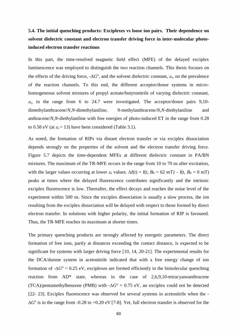
60

5.4. The initial quenching products: Exciplexes vs loose ion pairs. Their dependence on

solvent dielectric constant and electron transfer driving force in inter-molecular photo-

induced electron transfer reactions

In this part, the time-resolved magnetic field effect (MFE) of the delayed exciplex

luminescence was employed to distinguish the two reaction channels. This thesis focuses on

the effects of the driving force, -Go, and the solvent dielectric constant, s, on the prevalence

of the reaction channels. To this end, the different acceptor/donor systems in micro-

homogeneous solvent mixtures of propyl acetate/butyronitrile of varying dielectric constant,

s, in the range from 6 to 24.7 were investigated. The acceptor/donor pairs 9,10-

dimethylanthracene/N,N-dimethylaniline, 9-methylanthracene/N,N-diethylaniline and

anthracene/N,N-diethylaniline with free energies of photo-induced ET in the range from 0.28

to 0.58 eV (at s = 13) have been considered (Table 3.1).

As noted, the formation of RIPs via distant electron transfer or via exciplex dissociation

depends strongly on the properties of the solvent and the electron transfer driving force.

Figure 5.7 depicts the time-dependent MFEs at different dielectric constant in PA/BN

mixtures. The maximum of the TR-MFE occurs in the range from 10 to 70 ns after excitation,

with the larger values occurring at lower s values. I(t) = I(t, B0 = 62 mT) – I(t, B0 = 0 mT)

peaks at times where the delayed fluorescence contributes significantly and the intrinsic

exciplex fluorescence is low. Thereafter, the effect decays and reaches the noise level of the

experiment within 500 ns. Since the exciplex dissociation is usually a slow process, the ion

resulting from the exciplex dissociation will be delayed with respect to those formed by direct

electron transfer. In solutions with higher polarity, the initial formation of RIP is favoured.

Thus, the TR-MFE reaches its maximum at shorter times.

The primary quenching products are strongly affected by energetic parameters. The direct

formation of free ions, partly at distances exceeding the contact distance, is expected to be

significant for systems with larger driving force [10, 14, 20-21]. The experimental results for

the DCA/durene system in acetonitrile indicated that with a free energy change of ion

formation of -Go = 0.25 eV, exciplexes are formed efficiently in the bimolecular quenching

reaction from AD* state, whereas in the case of 2,6,9,10-tetracyanoanthracene

(TCA)/pentamethylbenzene (PMB) with -Go = 0.75 eV, an exciplex could not be detected

[22- 23]. Exciplex fluorescence was observed for several systems in acetonitrile when the -

Go is in the range from -0.28 to +0.20 eV [7-8]. Yet, full electron transfer is observed for the

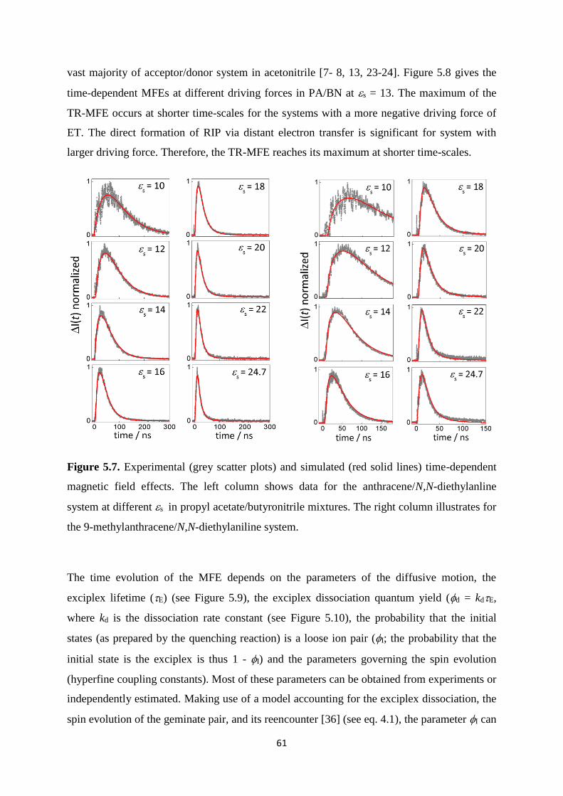
61

vast majority of acceptor/donor system in acetonitrile [7- 8, 13, 23-24]. Figure 5.8 gives the

time-dependent MFEs at different driving forces in PA/BN at s = 13. The maximum of the

TR-MFE occurs at shorter time-scales for the systems with a more negative driving force of

ET. The direct formation of RIP via distant electron transfer is significant for system with

larger driving force. Therefore, the TR-MFE reaches its maximum at shorter time-scales.

Figure 5.7. Experimental (grey scatter plots) and simulated (red solid lines) time-dependent

magnetic field effects. The left column shows data for the anthracene/N,N-diethylanline

system at different s in propyl acetate/butyronitrile mixtures. The right column illustrates for

the 9-methylanthracene/N,N-diethylaniline system.

The time evolution of the MFE depends on the parameters of the diffusive motion, the

exciplex lifetime (E) (see Figure 5.9), the exciplex dissociation quantum yield (d = kdE,

where kd is the dissociation rate constant (see Figure 5.10), the probability that the initial

states (as prepared by the quenching reaction) is a loose ion pair (I; the probability that the

initial state is the exciplex is thus 1 - I) and the parameters governing the spin evolution

(hyperfine coupling constants). Most of these parameters can be obtained from experiments or

independently estimated. Making use of a model accounting for the exciplex dissociation, the

spin evolution of the geminate pair, and its reencounter [36] (see eq. 4.1), the parameter I can

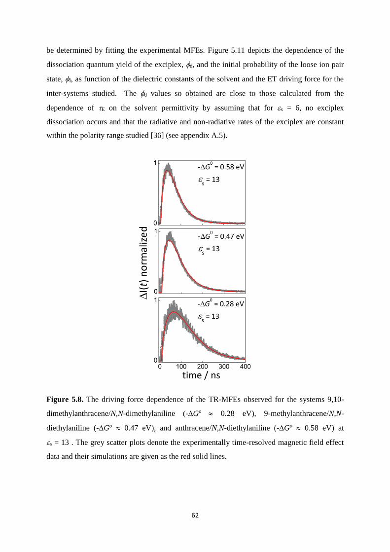
62

be determined by fitting the experimental MFEs. Figure 5.11 depicts the dependence of the

dissociation quantum yield of the exciplex, d, and the initial probability of the loose ion pair

state, I, as function of the dielectric constants of the solvent and the ET driving force for the

inter-systems studied. The d values so obtained are close to those calculated from the

dependence of E on the solvent permittivity by assuming that for s = 6, no exciplex

dissociation occurs and that the radiative and non-radiative rates of the exciplex are constant

within the polarity range studied [36] (see appendix A.5).

Figure 5.8. The driving force dependence of the TR-MFEs observed for the systems 9,10-

dimethylanthracene/N,N-dimethylaniline (-Go 0.28 eV), 9-methylanthracene/N,N-

diethylaniline (-Go 0.47 eV), and anthracene/N,N-diethylaniline (-Go 0.58 eV) at

s = 13 . The grey scatter plots denote the experimentally time-resolved magnetic field effect

data and their simulations are given as the red solid lines.

63

Figure 5.9. Solvent polarity dependence of the intrinsic exciplex lifetimes for the studied

inter-systems.

Figure 5.10. Solvent dependence of the dissociation rate constant for the studied inter-

systems.

From the data summarized in Figure 5.11, we infer that the exciplex quenching channels

contributes at all studied polarities, even for anthracene/N,N-diethylaniline, which exhibits the

most exergonic ET among the inter-system studied (-Go 0.58 eV). As expected, exciplex

formation is dominating at low polarities (for s < 15) and its significance increases with

decreasing ET driving force. Interestingly, however, for all system, I levels off upon

64

increasing the solvent dielectric constant (for s > 15) and the exciplex channel contributes

significantly even in pure butyronitrile (s = 24.7). d increases with increasing polarity of the

solutions. At low polarity, the exciplex formation (pathway 1A in Figure 2.16) is dominant.

This is in qualitative agreement with the model introduced in ref. 35, which predicts a more

stabilized exciplex at low polarity of the solvent environment – essentially a consequence of

the less shielded Coulomb interaction of A- and D+ in low-permittivity solvents. The initial

formation of the RIP is more favoured in polar solution, where the exciplex potential well is

less pronounced and the excited state population partly reacts through the loose-ion pair

channel prior to assuming the well-defined mutual orientation necessary for forming the

exciplex.

Figure 5.11. Solvent dependence of the initial probability of the loose ion pair state, I,

(upper panel) and the dissociation quantum yield of the exciplex, d, (lower panel) of the

systems 9,10-dimethylanthracene/N,N-dimethylaniline (red filled squares), 9-

methylanthracene/N,N-diethylaniline (grey filled triangles), and anthracene/N,N-diethylaniline

(blue filled circles) in propyl acetate/butyronitrile mixtures. The sole purpose of the solid lines

is to guide the eye; no physical model is implied.

The fact that the direct formation of loose ions via full electron transfer (pathway 1B in Figure

2.16) is more significant for systems with larger ET driving forces is a consequence of the

65

intrinsic ET rate constants increasing with driving force in the Marcus normal region [87-88].

Yet, even for the most polar solutions and the largest driving forces studied the two types of

ET reactions occur competitively. If the (long-distance) ET occurs faster than the diffusive

approach of A* and D, the acceptor excited state is deactivated by full ET. On the other hand,

if the diffusive approach giving rise to the favourable stacked configuration facilitating the

exciplex is faster than the (more) distant ET process, the exciplex channel dominates. This

also suggests that in solvents of comparable permittivity and electron transfer parameters, the

loose-ion channel will gain significance with increasing solvent viscosity. Work along the

lines of this supposition is underway. Apparently, for the low-viscous solvent system studied

here ( = 0.58 cP independent from composition), the diffusive approach to the stacking

distance is fast enough for the exciplex formation to always contribute significantly, even at s

20. Unfortunately, the approach detailed here cannot be easily extended to more polar

solutions as a consequence of the low emissivity of the exciplexes/tight ion pairs at dielectric

constants exceeding 25.

5.5. The initial quenching products: Exciplexes vs loose ion pairs. Their dependence on

solvent dielectric constant and chain length of Mant-n-O-2-DMA systems

All polymethylene-linked compounds synthesized to investigate the fluorescence quenching

mechanism in this thesis are completely new. No MFE results on these systems have been

described in the literature so far. Furthermore, the hyperfine coupling constants (HFCs) used

to calculate the spin evolution of the RIP have not been published yet. The experimental

measurements to get the HFCs and simulations of the time-resolved MFE data are in progress.

66

6. CONCLUSIONS AND OUTLOOKS

6.1. Conclusions

The polymethylene-linked acceptor/donor pairs have been synthesized. The magnitude of the

MFE of the exciplex of these compounds determined from steady-state and time-resolved

MFE measurements is larger than that of inter-systems. This can be attributed to an increase

of the probability of geminate reencounter between two radicals of RIP which generated via

intra-molecular photo-induced ET.

MFE dependence on solvent polarity and chain length has been investigated. For both

systems, the MFE of the exciplex is a function of the static dielectric constants, s. The onset

of the MFE in inter-systems is at s > 7 while that is at s > 10 in intra-systems. The maximum

MFE of linked-acceptor/donor exciplex attains at larger s value (s = 24.7) while that appears

around s = 18 for free diffusing systems. S-T conversion is impeded when the inter-radical

distance is small, i.e., the exchange interaction J(r) is large. This results in a decrease in the

MFE with decreasing chain length. When the chain length increases (n = 8, 10, 16), the

exchange interaction is negligible. S-T conversion is similar to the inter-systems, MFE thus

enhances.

By systematically varying the solvent polarity as well as the electron transfer driving forces

and using a model which accounts for the initial charge transfer state and the dissociation of

the exciplex, this work has been able to demonstrate that even in comparably polar solvents a

significant fraction of photo-excited acceptor/donor systems deactivates via direct exciplex

formation instead of full charge transfer. This conclusion has been reached based on TR-MFE

data and the observation that the MFE originating from the exciplex (by dissociation into a

RIP and its reencounter) lags the MFE resulting from loose ion pairs. The results can

contribute to the clarification of the question whether exciplexes can contribute to the charge

separation process even in polar media. This question is of relevance insofar as to date no

theoretical model is known that satisfactory bridges the domains of diabatic, solvent-

controlled outer-sphere electron transfer and that of exciplex formation. For the studied

systems, the initial RIP probability was always markedly less than unity. At low polarities,

and less negative driving force (-G0 0.28 eV), fluorescence is quenched predominantly by

67

forming an exciplex. At higher polarity and for more exergonic charge separation processes, a

RIP is the primary quenching product. Nonetheless, the exciplex formation remains important

even for -G0 0.58 eV and s = 24.7. Furthermore, the direct RIP formation is slightly more

significant for the system with larger ET driving force.

6.2. Outlooks

The experimental data from time-resolved MFE measurements will be simulated by

using the model in which the reversibility of RIP and exciplex is taken into account.

The scenario of the mechanism of fluorescence quenching via intra-molecular photo-

induced ET will be clarified.

In this thesis, there have been left space for many more interesting experiments. For

chain-linked systems, the fluorescence quenching mechanism and MFE should be

measured in micro-heterogeneous binary solvents (toluene/dimethylsulfoxide).

Hopefully, the preferential solvation effect will give the interesting results.

Observation of the initial quenching products by absorption transient spectroscopy in

time-scales of picosecond or femtosecond would be necessary.

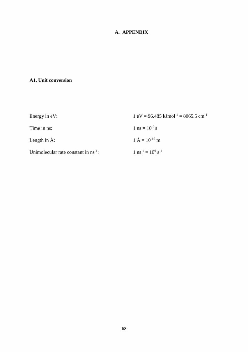
68

A. APPENDIX

A1. Unit conversion

Energy in eV: 1 eV = 96.485 kJmol-1 = 8065.5 cm-1

Time in ns: 1 ns = 10-9 s

Length in Å: 1 Å = 10-10 m

Unimolecular rate constant in ns-1: 1 ns-1 = 109 s-1

69

A2. 1H, 13C-NMR and mass spectra of Mant-n-O-2-DMA compounds

(a) 1H-NMR spectrum of 9-Bromo-10-methylanthracene

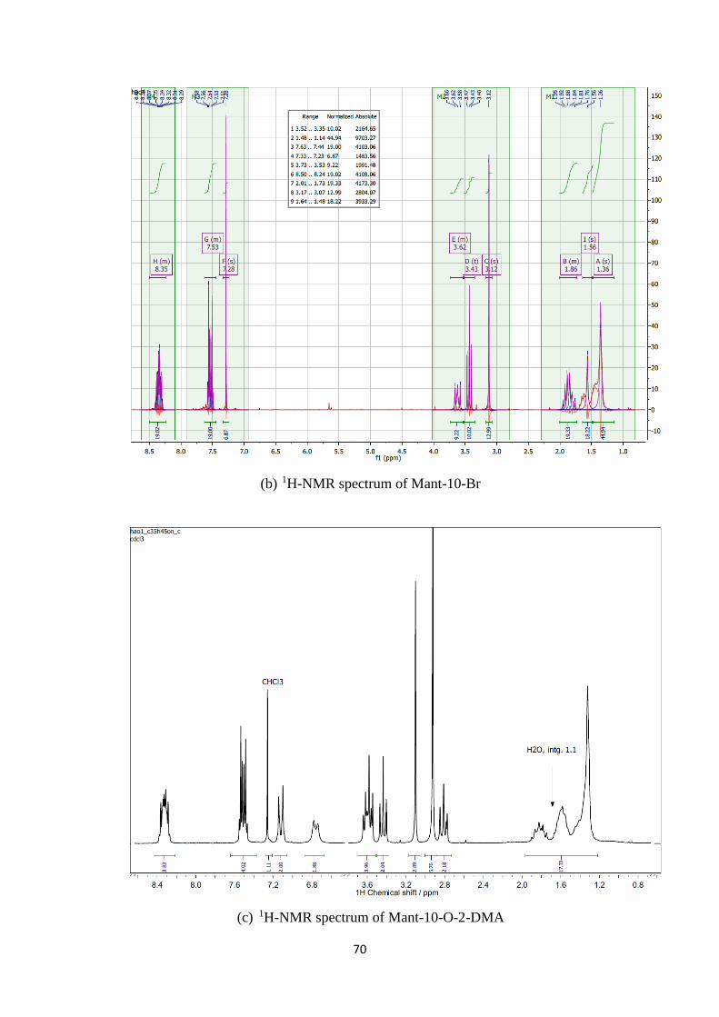
70

(b) 1H-NMR spectrum of Mant-10-Br

(c) 1H-NMR spectrum of Mant-10-O-2-DMA

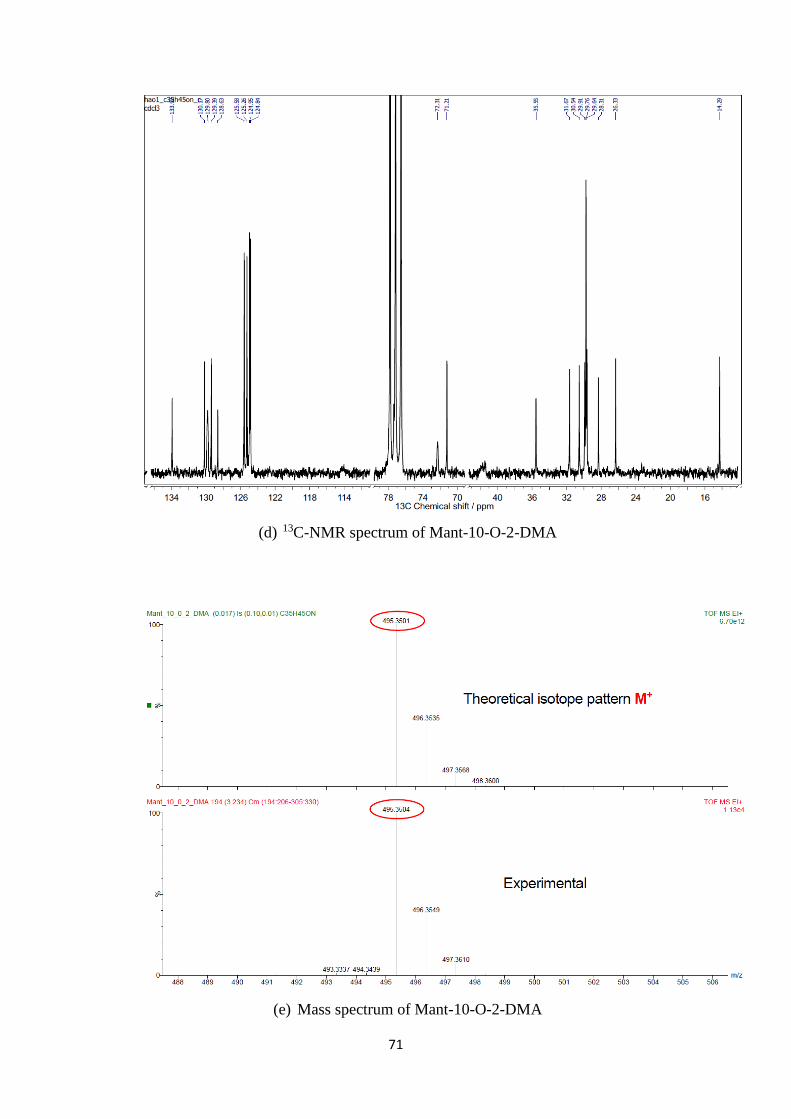
71

(d) 13C-NMR spectrum of Mant-10-O-2-DMA

(e) Mass spectrum of Mant-10-O-2-DMA

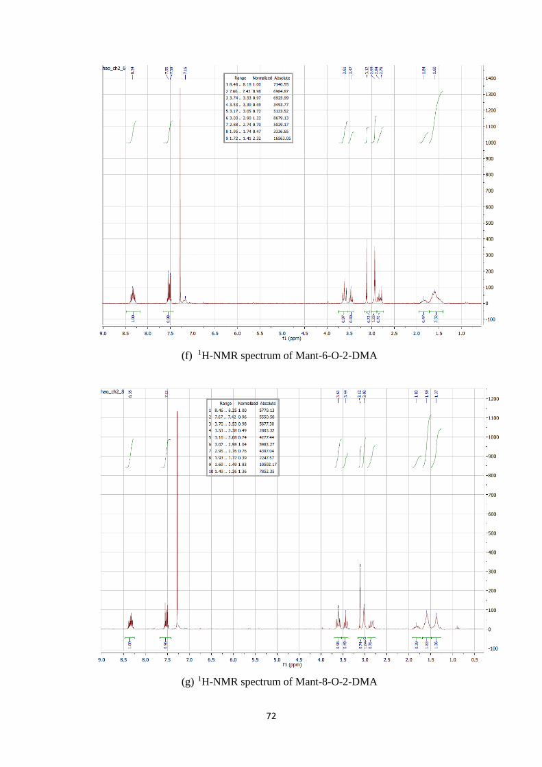
72

(f) 1H-NMR spectrum of Mant-6-O-2-DMA

(g) 1H-NMR spectrum of Mant-8-O-2-DMA

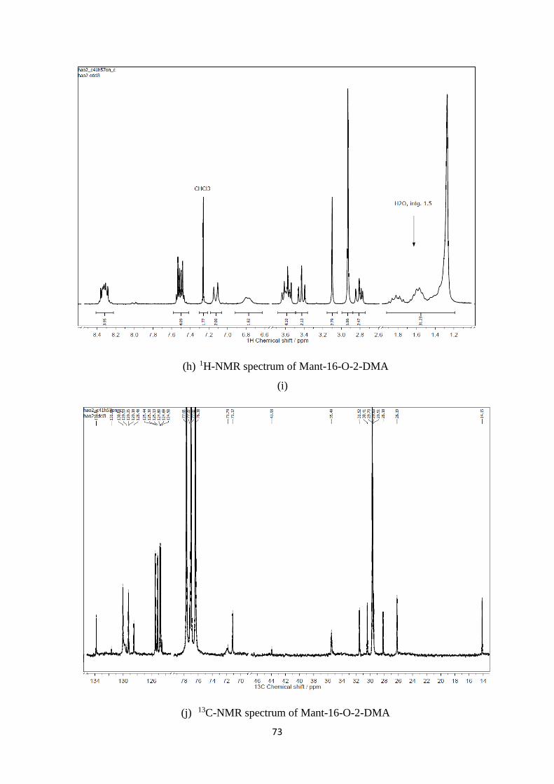
73

(h) 1H-NMR spectrum of Mant-16-O-2-DMA

(i)

(j) 13C-NMR spectrum of Mant-16-O-2-DMA

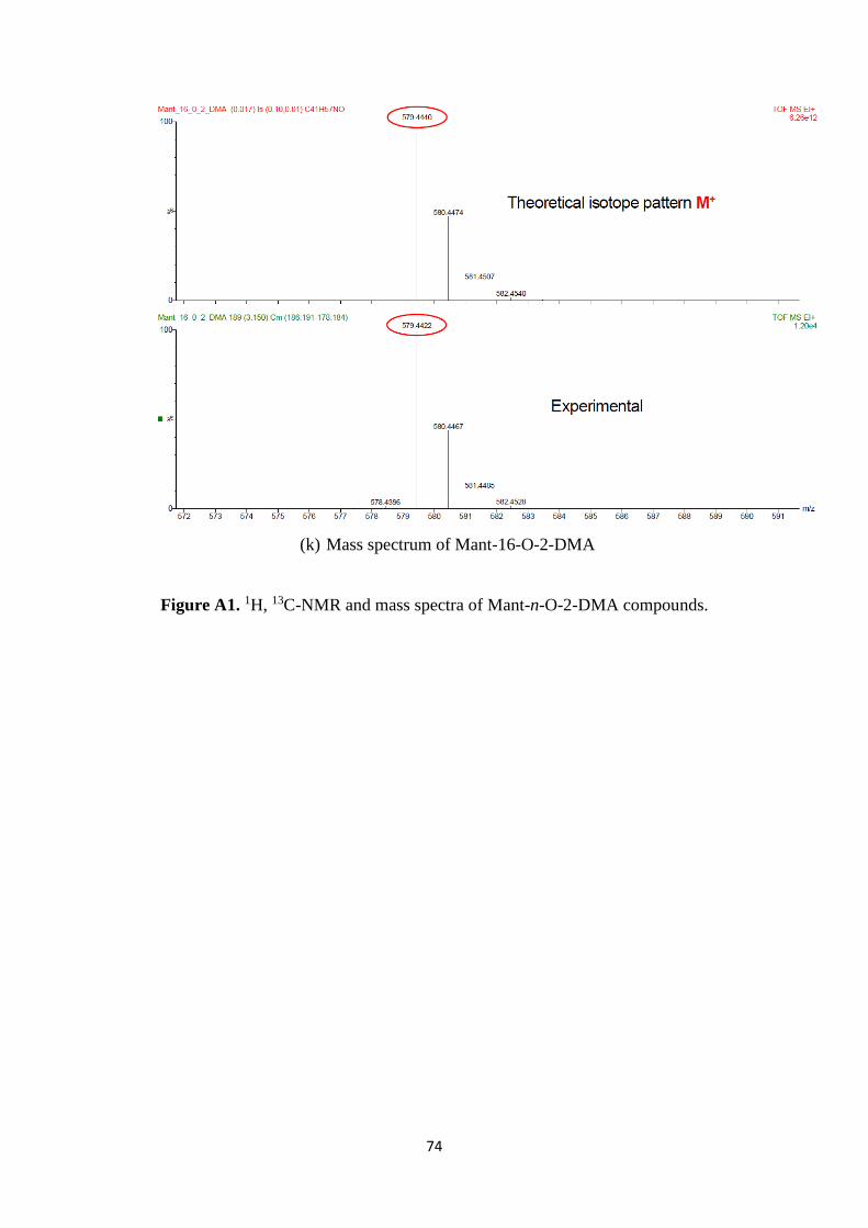
74

(k) Mass spectrum of Mant-16-O-2-DMA

Figure A1. 1H, 13C-NMR and mass spectra of Mant-n-O-2-DMA compounds.

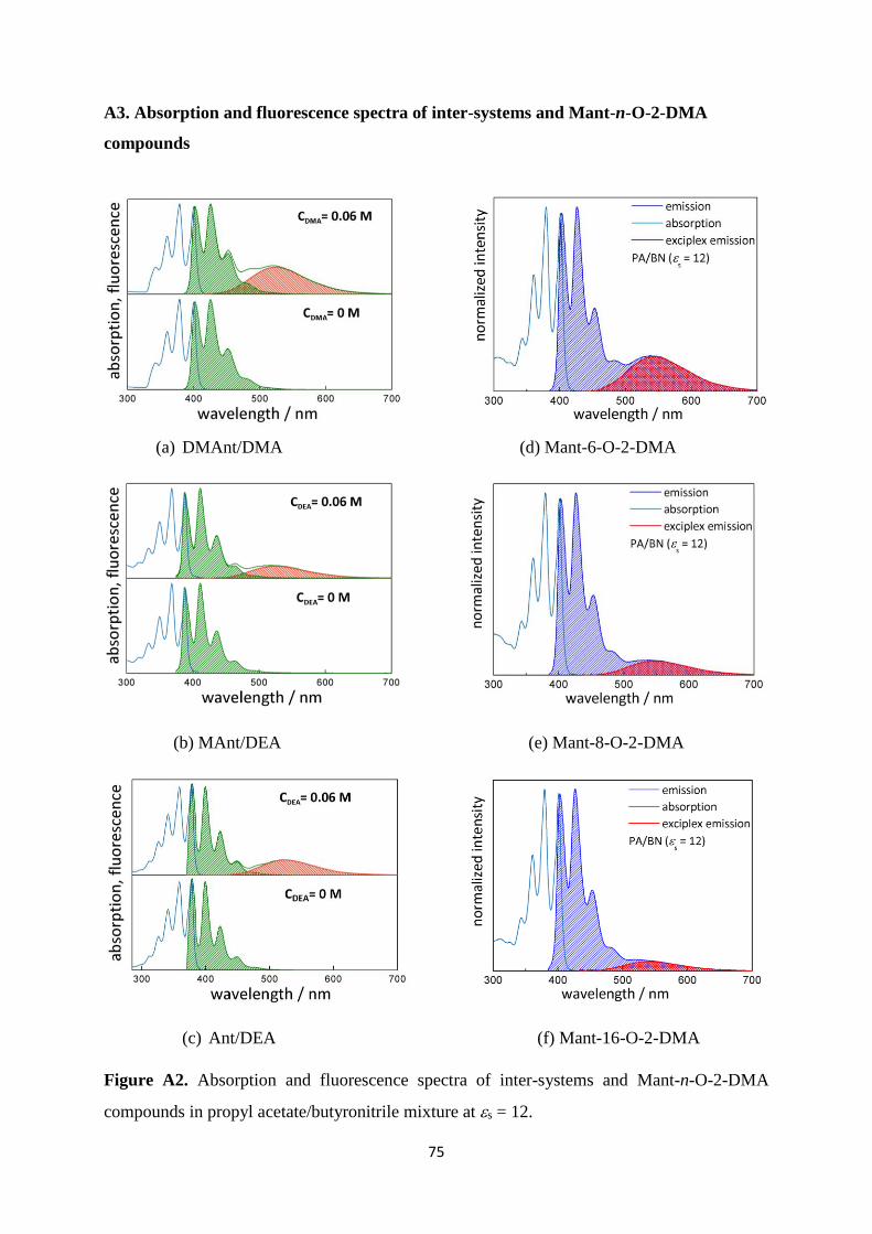
75

A3. Absorption and fluorescence spectra of inter-systems and Mant-n-O-2-DMA

compounds

(a) DMAnt/DMA (d) Mant-6-O-2-DMA

(b) MAnt/DEA (e) Mant-8-O-2-DMA

(c) Ant/DEA (f) Mant-16-O-2-DMA

Figure A2. Absorption and fluorescence spectra of inter-systems and Mant-n-O-2-DMA

compounds in propyl acetate/butyronitrile mixture at s = 12.

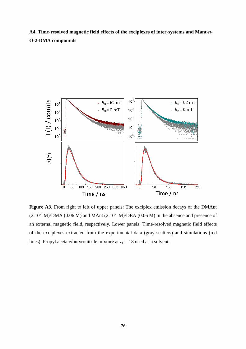
76

A4. Time-resolved magnetic field effects of the exciplexes of inter-systems and Mant-n-

O-2-DMA compounds

Figure A3. From right to left of upper panels: The exciplex emission decays of the DMAnt

(2.10-5 M)/DMA (0.06 M) and MAnt (2.10-5 M)/DEA (0.06 M) in the absence and presence of

an external magnetic field, respectively. Lower panels: Time-resolved magnetic field effects

of the exciplexes extracted from the experimental data (gray scatters) and simulations (red

lines). Propyl acetate/butyronitrile mixture at s = 18 used as a solvent.

77

(a) Mant-8-O-2-DMA exciplex

(b) Mant-10-O-2-DMA exciplex

Figure A4. Upper panels of (a) and (b): The exciplex emission decays of the Mant-8-O-2-

DMA (2.10-5 M) and Mant-10-O-2-DMA (2.10-5 M) in the absence and presence of an

external magnetic field, respectively. Lower panels of (a) and (b): Time-resolved magnetic

field effects of the exciplexes extracted from the experimental data (gray lines). Neat

butyronitrile (s = 24.7) used as a solvent.

78

A5. Formulation of the exciplex dissociation quantum yield, d

The exciplex lifetime is a function of static dielectric constant, s:

1( )

( )E s

r nr d sk k k

(A.1)

Here kr, knr are the rate constants of the radiative and non-radiative exciplex decays,

respectively. kd gives the exciplex dissociation rate constant.

At s = 6, under the assumption that there is no exciplex dissociation, i.e., kd = 0.

Introducing kd = 0 in eq. (A.1) yields

1

( 6)r nr

E s

k k const

(A.2)

From eq. (A.1) and eq. (A.2), we can calculate kd through:

1 1( )

( ) ( 6)d s

E s E s

k

(A.3)

The exciplex dissociation quantum yield is defined by:

( )( )

( )

d sd s

d s r nr

k

k k k

(A.4)

Introducing eq. (A.3) in eq. (A.4) yields

( ) ( ). ( )d s d s E sk (A.5)

79

ACRONYMS

Solvents

ACN : acetonitrile

BN : butyronitrile

EtCN : propionitrile

PA : propyl acetate

Substances

Ant : anthracence

DEA : N,N-diethylaniline

DMA : N,N-dimethylaniline

DMAnt : 9,10-dimethylanthracene

DMAPE : 2-[(4-dimethylamino)phenyl]ethanol

MAnt : 9-methylanthracene

1,6-DBH : 1,6-dibromohexane

1,8-DBO : 1,8-dibromooctane

1,10-DBD : 1,10-dibromodecane

1,16-HDDO : 1,16-hexadecanediol

1,16-DBHD : 1,16- dibromohexadecane

Mant-6-Br : 1-bromo-6-[9-(10-methyl)anthryl]hexane

Mant-8-Br : 1-bromo-8-[9-(10-methyl)anthryl]octane

Mant-10-Br : 1-bromo-10-[9-(10-methyl)anthryl]decane

Mant-16-Br : 1-bromo-16-[9-(10-methyl)anthryl]hexadecane

Mant-6-O-2-DMA : 2-[4-(dimethylamino)phenyl]ethyl 6-[9-(10-methyl)anthryl]hexyl

ether

Mant-8-O-2-DMA : 2-[4-(dimethylamino)phenyl]ethyl 8-[9-(10-methyl)anthryl]octyl ether

Mant-10-O-2-DMA : 2-[4-(dimethylamino)phenyl]ethyl 10-[9-(10-methyl)anthryl]decyl

ether

Mant-16-O-2-DMA : 2-[4-(dimethylamino)phenyl]ethyl 16-[9-(10-

methyl)anthryl]hexadecyl ether

80

Others

A : acceptor

D : donor

ET : electron transfer

GS : ground state

HFI : hyperfine interaction

LE : locally excited

LIP : loose ion pair

MFE : magnetic field effect

PET : photo-induced electron transfer

P : product

R : reactant

RIP : radical ion pair

S : singlet

SRIP : singlet radical ion pair

SS : steady-state

T : triplet

TCSPC : time-correlated single photon-counting

TR : time-resolved

TR-MFE : time-resolved magnetic field effect

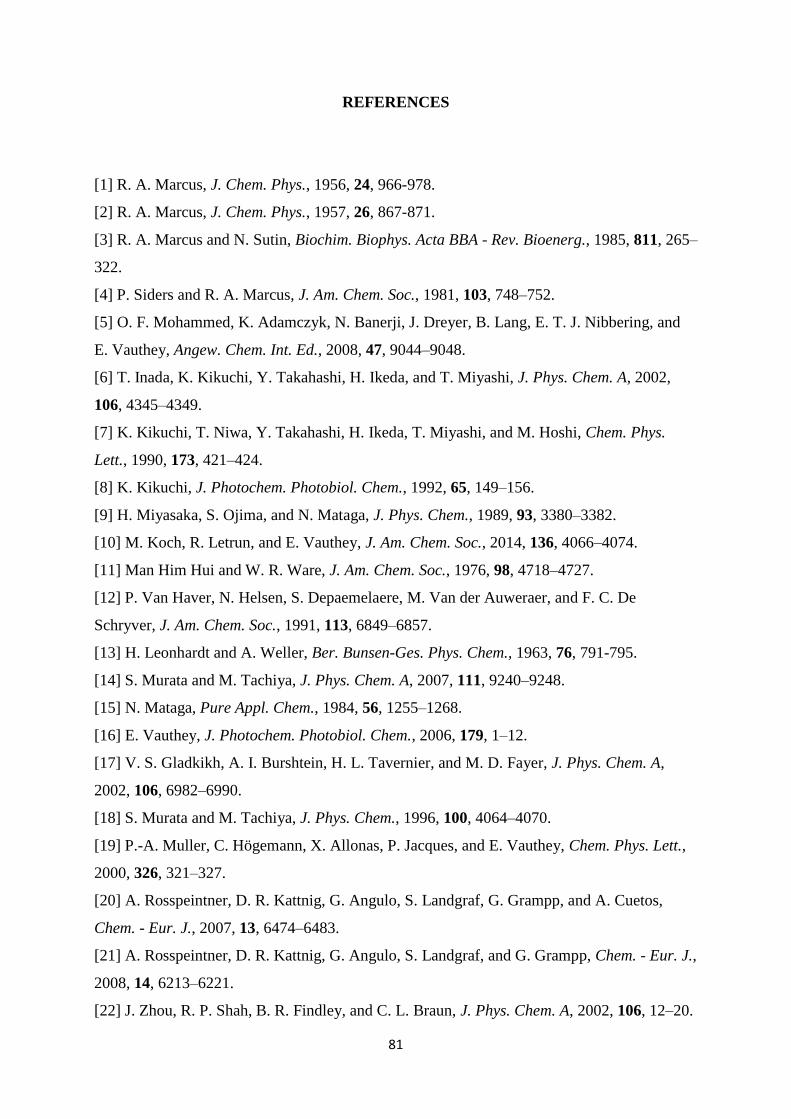
81

REFERENCES

[1] R. A. Marcus, J. Chem. Phys., 1956, 24, 966-978.

[2] R. A. Marcus, J. Chem. Phys., 1957, 26, 867-871.

[3] R. A. Marcus and N. Sutin, Biochim. Biophys. Acta BBA - Rev. Bioenerg., 1985, 811, 265–

322.

[4] P. Siders and R. A. Marcus, J. Am. Chem. Soc., 1981, 103, 748–752.

[5] O. F. Mohammed, K. Adamczyk, N. Banerji, J. Dreyer, B. Lang, E. T. J. Nibbering, and

E. Vauthey, Angew. Chem. Int. Ed., 2008, 47, 9044–9048.

[6] T. Inada, K. Kikuchi, Y. Takahashi, H. Ikeda, and T. Miyashi, J. Phys. Chem. A, 2002,

106, 4345–4349.

[7] K. Kikuchi, T. Niwa, Y. Takahashi, H. Ikeda, T. Miyashi, and M. Hoshi, Chem. Phys.

Lett., 1990, 173, 421–424.

[8] K. Kikuchi, J. Photochem. Photobiol. Chem., 1992, 65, 149–156.

[9] H. Miyasaka, S. Ojima, and N. Mataga, J. Phys. Chem., 1989, 93, 3380–3382.

[10] M. Koch, R. Letrun, and E. Vauthey, J. Am. Chem. Soc., 2014, 136, 4066–4074.

[11] Man Him Hui and W. R. Ware, J. Am. Chem. Soc., 1976, 98, 4718–4727.

[12] P. Van Haver, N. Helsen, S. Depaemelaere, M. Van der Auweraer, and F. C. De

Schryver, J. Am. Chem. Soc., 1991, 113, 6849–6857.

[13] H. Leonhardt and A. Weller, Ber. Bunsen-Ges. Phys. Chem., 1963, 76, 791-795.

[14] S. Murata and M. Tachiya, J. Phys. Chem. A, 2007, 111, 9240–9248.

[15] N. Mataga, Pure Appl. Chem., 1984, 56, 1255–1268.

[16] E. Vauthey, J. Photochem. Photobiol. Chem., 2006, 179, 1–12.

[17] V. S. Gladkikh, A. I. Burshtein, H. L. Tavernier, and M. D. Fayer, J. Phys. Chem. A,

2002, 106, 6982–6990.

[18] S. Murata and M. Tachiya, J. Phys. Chem., 1996, 100, 4064–4070.

[19] P.-A. Muller, C. Högemann, X. Allonas, P. Jacques, and E. Vauthey, Chem. Phys. Lett.,

2000, 326, 321–327.

[20] A. Rosspeintner, D. R. Kattnig, G. Angulo, S. Landgraf, G. Grampp, and A. Cuetos,

Chem. - Eur. J., 2007, 13, 6474–6483.

[21] A. Rosspeintner, D. R. Kattnig, G. Angulo, S. Landgraf, and G. Grampp, Chem. - Eur. J.,

2008, 14, 6213–6221.

[22] J. Zhou, R. P. Shah, B. R. Findley, and C. L. Braun, J. Phys. Chem. A, 2002, 106, 12–20.

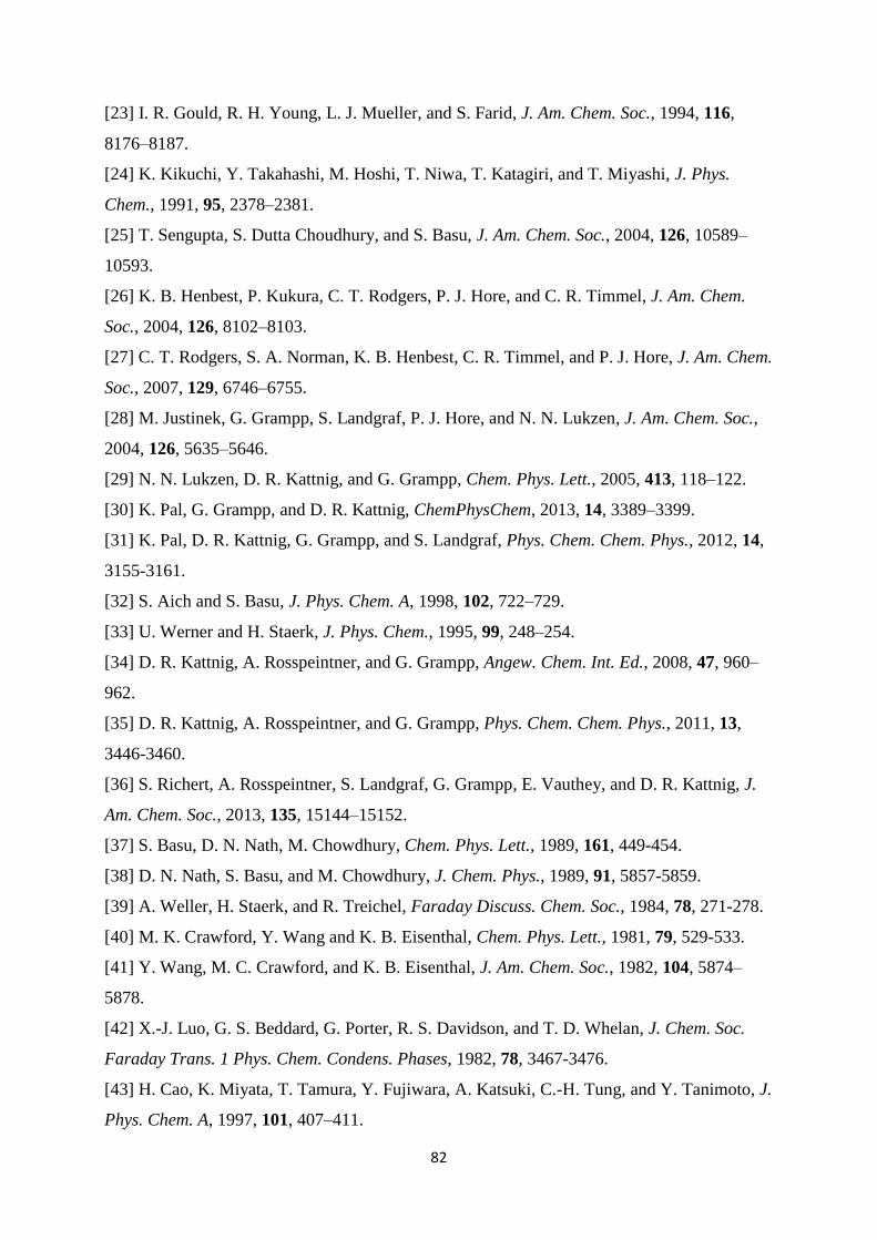
82

[23] I. R. Gould, R. H. Young, L. J. Mueller, and S. Farid, J. Am. Chem. Soc., 1994, 116,

8176–8187.

[24] K. Kikuchi, Y. Takahashi, M. Hoshi, T. Niwa, T. Katagiri, and T. Miyashi, J. Phys.

Chem., 1991, 95, 2378–2381.

[25] T. Sengupta, S. Dutta Choudhury, and S. Basu, J. Am. Chem. Soc., 2004, 126, 10589–

10593.

[26] K. B. Henbest, P. Kukura, C. T. Rodgers, P. J. Hore, and C. R. Timmel, J. Am. Chem.

Soc., 2004, 126, 8102–8103.

[27] C. T. Rodgers, S. A. Norman, K. B. Henbest, C. R. Timmel, and P. J. Hore, J. Am. Chem.

Soc., 2007, 129, 6746–6755.

[28] M. Justinek, G. Grampp, S. Landgraf, P. J. Hore, and N. N. Lukzen, J. Am. Chem. Soc.,

2004, 126, 5635–5646.

[29] N. N. Lukzen, D. R. Kattnig, and G. Grampp, Chem. Phys. Lett., 2005, 413, 118–122.

[30] K. Pal, G. Grampp, and D. R. Kattnig, ChemPhysChem, 2013, 14, 3389–3399.

[31] K. Pal, D. R. Kattnig, G. Grampp, and S. Landgraf, Phys. Chem. Chem. Phys., 2012, 14,

3155-3161.

[32] S. Aich and S. Basu, J. Phys. Chem. A, 1998, 102, 722–729.

[33] U. Werner and H. Staerk, J. Phys. Chem., 1995, 99, 248–254.

[34] D. R. Kattnig, A. Rosspeintner, and G. Grampp, Angew. Chem. Int. Ed., 2008, 47, 960–

962.

[35] D. R. Kattnig, A. Rosspeintner, and G. Grampp, Phys. Chem. Chem. Phys., 2011, 13,

3446-3460.

[36] S. Richert, A. Rosspeintner, S. Landgraf, G. Grampp, E. Vauthey, and D. R. Kattnig, J.

Am. Chem. Soc., 2013, 135, 15144–15152.

[37] S. Basu, D. N. Nath, M. Chowdhury, Chem. Phys. Lett., 1989, 161, 449-454.

[38] D. N. Nath, S. Basu, and M. Chowdhury, J. Chem. Phys., 1989, 91, 5857-5859.

[39] A. Weller, H. Staerk, and R. Treichel, Faraday Discuss. Chem. Soc., 1984, 78, 271-278.

[40] M. K. Crawford, Y. Wang and K. B. Eisenthal, Chem. Phys. Lett., 1981, 79, 529-533.

[41] Y. Wang, M. C. Crawford, and K. B. Eisenthal, J. Am. Chem. Soc., 1982, 104, 5874–

5878.

[42] X.-J. Luo, G. S. Beddard, G. Porter, R. S. Davidson, and T. D. Whelan, J. Chem. Soc.

Faraday Trans. 1 Phys. Chem. Condens. Phases, 1982, 78, 3467-3476.

[43] H. Cao, K. Miyata, T. Tamura, Y. Fujiwara, A. Katsuki, C.-H. Tung, and Y. Tanimoto, J.

Phys. Chem. A, 1997, 101, 407–411.

83

[44] Y. Tanimoto, N. Okada, M. Itoh, K. Iwai, K. Sugioka, F. Takemura, R.i Nakagaki, and S.

Nagakura, Chem. Phys. Lett, 1987, 136, 42-74.

[45] H. Cao, Y. Fujiwara, T. Haino, Y. Fukazawa, C-H. Tung, and Y. Tanimoto, Bull. Chem.

Soc. Jpn, 1996, 69, 2801-2813.

[46] S. Arrhenius, Zeit. physikal. Chem, 1889, 4, 226–48.

[47] H. M. Rosenstock, M. B. Wallenstein, A. L. Wahrhaftig, H. Eyring, Proc. Natl.

Acad. Sci. U. S. A, 1952, 38, 667–78.

[48] J. C. Giddings, H. Eyring, H, J. Chem. Phys, 1954, 22, 538–42.

[49] D. G. Truhlar, B. C. Garrett, and S. J. Klippenstein, J. Phys. Chem., 1996, 100, 12771–

12800.

[50] N. Sutin, Acc. Chem. Res, 1982, 15, 275–282.

[51] K. J. Laidler, Chemical Kinetics. 3rd ed; Prentice Hall, 1987; Vol. 3rd, p 531.

[52] A. Mansha, PhD thesis, Graz University of Technology, 2009.

[53] T. X. Nguyen, PhD thesis, Graz University of Technology, 2011.

[54] A. Rosspeintner, PhD thesis, Graz University of Technology, 2008.

[55] G. J. Kavarnos, Fundamentals of Photoinduced Electron Transfer; VCH Publishers: New

York, NY, 1993.

[56] R. A. Marcus, J. Chem. Phys., 1965, 43, 679-701.

[57] R. A. Marcus, J. Chem. Phys., 1956, 24, 979-989.

[58] G. L. Closs, L. T. Calcaterra, N. J. Green, K. W. Penfield, and J. R. Miller, J. Phys.

Chem., 1986, 90, 3673–3683.

[59] E. Vauthey, J. Phys. Chem. A, 2001, 105, 340–348.

[60] M. R. Wasielewski, M. P. Niemczyk, W. A. Svec, and E. B. Pewitt, J. Am. Chem. Soc.,

1985, 107, 1080–1082.

[61] N. Mataga, Y. Kanda, and T. Okada, J. Phys. Chem., 1986, 90, 3880–3882.

[62] R. A. Marcus, Disc. Faraday Soc, 1960, 29, 21-31.

[63] M. Justinek, PhD thesis, Graz University of Technology, 2003.

[64] H. Hayashi, Introduction to dynamic spin chemistry: magnetic field effects on chemical

and biochemical reactions, World Scientific, River Edge, N.J, 2004.

[65] H. Staerk, W. Kühnle, R. Treichel, A. Weller, Chem. Phys. Lett. 1985, 118, 19-24.

[66] J. R. Lakowicz, Principles of fluorescence spectroscopy, Springer, New York, 3rd ed.,

2006.

[67] M. Montalti and S. L. Murov, Eds., Handbook of photochemistry, CRC/Taylor &

Francis, Boca Raton, 3rd ed., 2006.

84

[68] D. Mosnaim, D.C. Nonhebel, J.A. Russell, Tetrahedron, 1969, 25, 3485-3492.

[69] S. Franceschi, V. Andreu, N. de Viguerie, M. Riviere, A. Lattes, and A. Moisand, New J.

Chem., 1998, 22, 225–231.

[70] J. A. Riddick, Organic solvents: physical properties and methods of purification, Wiley,

New York, 4th ed., 1986.

[71] M. G. Kuzmin, I. V. Soboleva, and E. V. Dolotova, J. Phys. Chem. A, 2007, 111, 206–

215.

[72] J. Bolton, A. Carrington, A. McLachlan, Mol. Phys, 1962, 5, 31-41.

[73] F. Gerson, W. Huber, Electron Spin Resonance Spectroscopy for Organic Radicals, 1st

ed.; Wiley-VCH, 2001.

[74] V. R. Gorelik, E. G. Bagryanskaya, N. N. Lukzen, I. V. Koptyug, V. V. Perov, and R. Z.

Sagdeev, J. Phys. Chem., 1996, 100, 5800–5807.

[75] S. F. Swallen, K. Weidemaier, and M. D. Fayer, J. Chem. Phys., 1996, 104, 2976.

[76] U. E. Steiner and T. Ulrich, Chem. Rev., 1989, 89, 51–147.

[77] P. Suppan, J. Chem. Soc. Faraday Trans. 1 Phys. Chem. Condens. Phases, 1987, 83,

495-509.

[78] P. Suppan, J. Photochem. Photobiol. A, 1990, 50, 293-330.

[79] Y. Tanimoto, K. Hasegawa, N. Okada, M. Itoh, K. Iwai, K. Sugioka, F. Takemura, R.

Nakagaki, and S. Nagakura, J. Phys. Chem., 1989, 93, 3586–3594.

[80] H. Lee, N. Yang, and A. E. Cohen, Nano Lett., 2011, 11, 5367–5372.

[81] Y. Tanimoto, M. Takashima, and M. Itoh, Bull. Chem. Soc. Jpn., 1989, 62, 3923-3931.

[82] A. Weller, F. Nolting, and H. Staerk, Chem. Phys. Lett., 1983, 96, 24–27.

[83] A. I. Shushin, Chem. Phys. Lett., 1991, 181, 274–278.

[84] J. B. Birks in Photophysics of Aromatic Molecules (Ed.: J. B. Birks),Wiley-Interscience,

London, 1970 (Wiley Monographs in Chemical Physics).

[85] N. K. Petrov, A. Wiessner, T. Fiebig, and H. Staerk, Chem. Phys. Lett., 1995, 241, 127–

132.

[86] N. K. Petrov, High Energy Chem., 2006, 40, 22–34.

[87] R. A. Marcus, Annu. Rev. Phys. Chem., 1964, 15, 155–196.

[88] N. Sutin, J. Photochem., 1979, 10, 19–40.