Anchoring Vignettes for Interpersonally Incomparable ...

Anchoring Vignettes for Interpersonally IncomparableSurvey Responses

Gary King

http://GKing.Harvard.Edu

January 18, 2007

Gary King () Anchoring Vignettes for Interpersonally Incomparable Survey Responseshttp://GKing.Harvard.Edu January 18, 2007 1

/ 27

Readings

Gary King and Jonathan Wand. “Comparing Incomparable SurveyResponses: Evaluating and Selecting Anchoring Vignettes,” PoliticalAnalysis, 15, 1 (Winter, 2007): 46–66.

Gary King; Christopher J.L. Murray; Joshua A. Salomon; and AjayTandon. “Enhancing the Validity and Cross-cultural Comparability ofMeasurement in Survey Research,” American Political ScienceReview, Vol. 98, No. 1 (February, 2004): 191–207.

Papers, FAQ, examples, software, conferences, videos:http://GKing.Harvard.edu/vign

Gary King () Anchoring Vignettes 2 / 27

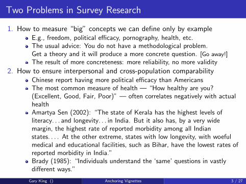
Two Problems in Survey Research

1. How to measure “big” concepts we can define only by exampleE.g., freedom, political efficacy, pornography, health, etc.The usual advice: You do not have a methodological problem.Get a theory and it will produce a more concrete question. [Go away!]

The result of more concreteness: more reliability, no more validity

2. How to ensure interpersonal and cross-population comparabilityChinese report having more political efficacy than AmericansThe most common measure of health — “How healthy are you?(Excellent, Good, Fair, Poor)” — often correlates negatively with actualhealthAmartya Sen (2002): “The state of Kerala has the highest levels ofliteracy. . . and longevity. . . in India. But it also has, by a very widemargin, the highest rate of reported morbidity among all Indianstates. . . . At the other extreme, states with low longevity, with woefulmedical and educational facilities, such as Bihar, have the lowest rates ofreported morbidity in India.”Brady (1985): “Individuals understand the ‘same’ questions in vastlydifferent ways.”


Anchoring Vignettes & Self-Assessments:Political Efficacy (about voting)

“[Alison] lacks clean drinking water. She and her neighbors are supporting anopposition candidate in the forthcoming elections that has promised to address theissue. It appears that so many people in her area feel the same way that theopposition candidate will defeat the incumbent representative.”

“[Jane] lacks clean drinking water because the government is pursuing anindustrial development plan. In the campaign for an upcoming election, anopposition party has promised to address the issue, but she feels it would be futileto vote for the opposition since the government is certain to win.”

“[Moses] lacks clean drinking water. He would like to change this, but he can’tvote, and feels that no one in the government cares about this issue. So he suffersin silence, hoping something will be done in the future.”

How much say [does ‘name’ / do you] have in getting the government to address issues

that interest [him / her / you]?

(a) Unlimited say, (b) A lot of say, (c) Some say, (d) Little say, (e) No say at all


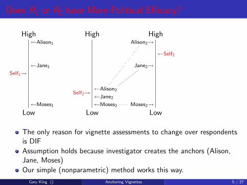
Does R1 or R2 have More Political Efficacy?

High←Alison1

←Jane1

Self1→

←Moses1

High

←Alison2

←Jane2Self2→

←Moses2

HighAlison2→

Jane2→

←Self2

Moses2→Low Low Low

The only reason for vignette assessments to change over respondentsis DIF

Assumption holds because investigator creates the anchors (Alison,Jane, Moses)

Our simple (nonparametric) method works this way.


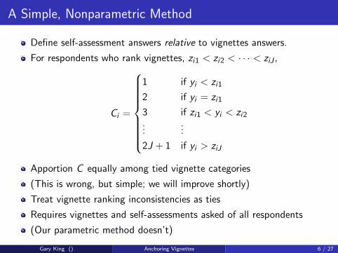
A Simple, Nonparametric Method

Define self-assessment answers relative to vignettes answers.

For respondents who rank vignettes, zi1 < zi2 < · · · < ziJ ,

Ci =

1 if yi < zi1

2 if yi = zi1

3 if zi1 < yi < zi2...

...

2J + 1 if yi > ziJ

Apportion C equally among tied vignette categories

(This is wrong, but simple; we will improve shortly)

Treat vignette ranking inconsistencies as ties

Requires vignettes and self-assessments asked of all respondents

(Our parametric method doesn’t)


Comparing China and Mexico


Mexico

Opposition leader Vicente Fox elected President.71-year rule of PRI party ends.

Peaceful transition of power begins.

Plenty of political efficacy


China: How much say do you have in getting thegovernment to address issues that interest you?


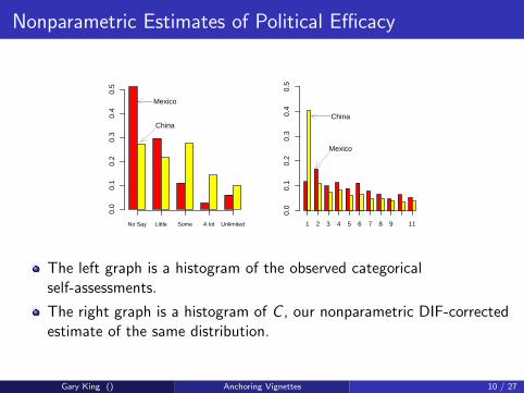
Nonparametric Estimates of Political Efficacy

No Say Little Some A lot Unlimited

Mexico

China

0.0

0.1

0.2

0.3

0.4

0.5

1 2 3 4 5 6 7 8 9 11

Mexico

China

0.0

0.1

0.2

0.3

0.4

0.5

The left graph is a histogram of the observed categoricalself-assessments.

The right graph is a histogram of C , our nonparametric DIF-correctedestimate of the same distribution.


Key Measurement Assumptions

1. Response Consistency: Each respondent uses the self-assessment andvignette categories in approximately the same way across questions.(DIF occurs across respondents, not across questions for any onerespondent.)

2. Vignette Equivalence:

(a) The actual level for any vignette is the same for all respondents.(b) The quantity being estimated exists.(c) The scale being tapped is perceived as unidimensional.

3. In other words: we allow response-category DIF but assume stemquestion equivalence.


Ties and Inconsistencies Produce Ranges

Survey 1: 2: 3: 4: 5:Example Responses y < z1 y = z1 z1 < y < z2 y = z2 y > z2 C1 y < z1 < z2 T {1}2 y = z1 < z2 T {2}3 z1 < y < z2 T {3}4 z1 < y = z2 T {4}5 z1 < z2 < y T {5}Ties:6 y < z1 = z2 T {1}7 y = z1 = z2 T T {2,3,4}8 z1 = z2 < y T {5}Inconsistencies:9 y < z2 < z1 T {1}10 y = z2 < z1 T T {1,2,3,4}11 z2 < y < z1 T T {1,2,3,4,5}12 z2 < y = z1 T T {2,3,4,5}13 z2 < z1 < y T {5}


Analyzing the DIF-Free Variable: More Efficiencies

How to analyze a variable with scalar and vector responses?

Define an unobserved variable: Yi ∼ Normal(xiβ, 1)

With observation mechanism, for scalar C , the same as ordered probit:

Ci = c if τc−1 ≤ Yi < τc

Probability of observing category c , for X = x0:

Pr(C = c |x0) =

∫ τc

τc−1

Normal(y |x0β, 1)dy

Observation mechanism for vector valued C :

Ci = c if τmin(c)−1 ≤ Yi < τmax(c)


Robust Analysis via Conditional Model

Condition on observed value of ci :

Pr(C = c |x0, ci ) =

{ Pr(C=c|x0)Pa∈ci

Pr(C=a|x0)for c ∈ ci

0 otherwise

Advantages compared to unconditional probabilities:

Conditions on ci by normalizing the probability to sum to one withinthe set ci and zero outside that set.For scalar values of ci , this expression simply returns the observedcategory: Pr(C = c |xi , ci ) = 1 for category c and 0 otherwise.For vector valued ci , it puts probability density over categories withinci , which in total sum to one.Probabilities can be interpreted for causal effects or summed toproduce a histogram.Result:

highly robust to model mispecification,extracts considerably more information from anchoring vignette data.


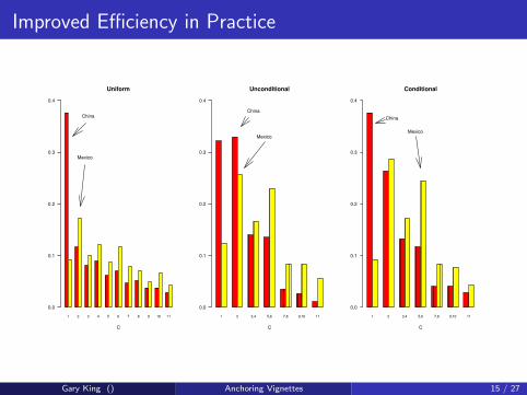
Improved Efficiency in Practice

1 2 3 4 5 6 7 8 9 10 11

Uniform

C

0.0

0.1

0.2

0.3

0.4

Mexico

China

1 2 3,4 5,6 7,8 9,10 11

Unconditional

C

0.0

0.1

0.2

0.3

0.4

Mexico

China

1 2 3,4 5,6 7,8 9,10 11

Conditional

C

0.0

0.1

0.2

0.3

0.4

Mexico

China


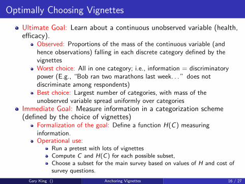
Optimally Choosing Vignettes

Ultimate Goal: Learn about a continuous unobserved variable (health,efficacy).

Observed: Proportions of the mass of the continuous variable (andhence observations) falling in each discrete category defined by thevignettesWorst choice: All in one category; i.e., information = discriminatorypower (E.g., “Bob ran two marathons last week. . . ” does notdiscriminate among respondents)Best choice: Largest number of categories, with mass of theunobserved variable spread uniformly over categories

Immediate Goal: Measure information in a categorization scheme(defined by the choice of vignettes)

Formalization of the goal: Define a function H(C ) measuringinformation.Operational use:

Run a pretest with lots of vignettesCompute C and H(C) for each possible subset,Choose a subset for the main survey based on values of H and cost ofsurvey questions.


Step 1: Criteria for Defining H(C ) for scalar C

Summarize C with a histogram, so H(C ) = H(p1, . . . , p2J+1). Add 3criteria:

1. H(0, 1, 0, 0, 0) = 0, i.e., when all mass is in (any) one category and at amaximum when p1 = p2 = · · · = p2J+1

2. H is a monotonically increasing function of the number of vignettes J(and hence 2J + 1, the number categories of C ).

3. Assume consistent decomposition:With one vignette, C has 3 categories (below, equal to, or above thevignette) and proportions p1 + p2 + q = 1Add a new vignette and we can decompose the “above” category (intobetween the two vignettes, equal to the second, or above the second).We now have 5 categories, with proportions p1 + p2 + p3 + p4 + p5 = 1.The information in the union of the smaller bins (3,4,5) should equalthat in the original undecomposed bin since q = p3 + p4 + p5.The information in the unaffected bins (1, 2) should remain the samewith the addition of the new vignette.More formally: H(p1, p2, p3, p4, p5) = H(p1, p2, q) + qH(p3, p4, p5)


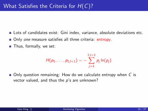
What Satisfies the Criteria for H(C )?

Lots of candidates exist: Gini index, variance, absolute deviations etc.

Only one measure satisfies all three criteria: entropy.

Thus, formally, we set:

H(p1, . . . , p2J+1) = −2J+1∑j=1

pj ln(pj)

Only question remaining: How do we calculate entropy when C isvector valued, and thus the p’s are unknown?


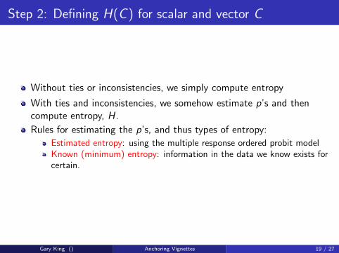
Step 2: Defining H(C ) for scalar and vector C

Without ties or inconsistencies, we simply compute entropy

With ties and inconsistencies, we somehow estimate p’s and thencompute entropy, H.

Rules for estimating the p’s, and thus types of entropy:

Estimated entropy: using the multiple response ordered probit modelKnown (minimum) entropy: information in the data we know exists forcertain.


Estimated Entropy

Measures the informativeness of the vignettes,

as supplemented by the predictive information in the covariates

A reasonable approach, uses a modification of a standard statisticalmodel, and robust to misspecification.

But it assumes the probit specification is correct. Normally this is ok,but decisions here are more consequential since they affect datacollection decisions and thus can preclude asking some questions

Thus, we also want “known entropy”.


Computing Known Entropy (no assumptions required)

Scalar-valued Ci observations are set to observed values.

Vector-valued Ci :

Elements of all possible vector responses are parameterized: (e.g.,p1, p2, p3 for Ci = {2, 3, 4})All mass is restricted to within the vector (e.g., p1 + p2 + p3 = 1)Choose all p’s to minimize entropy (i.e., adjust the p’s to see how spikythe distribution can become)Some tricks make this easy with a genetic optimizer.

Then form the histogram (summing the p’s) and compute entropy.

We now compute estimated entropy and known entropy for all possiblesubsets of vignettes.


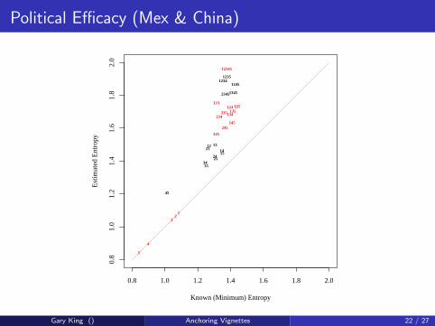
Political Efficacy (Mex & China)

0.8 1.0 1.2 1.4 1.6 1.8 2.0

0.8

1.0

1.2

1.4

1.6

1.8

2.0

Known (Minimum) Entropy

Est

imat

ed E

ntro

py

12

3

4

5

123124125

134135

145

234235

245

345

12345

12 131415

23

24253435

45

12341235

1245

13452345


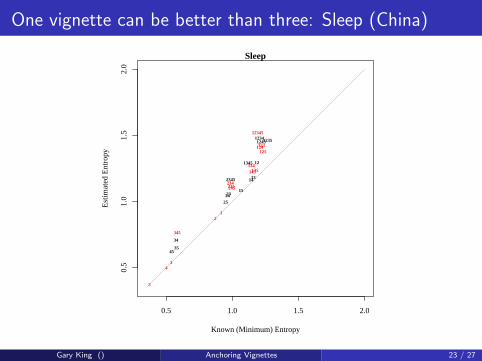
One vignette can be better than three: Sleep (China)

0.5 1.0 1.5 2.0

0.5

1.0

1.5

2.0

Sleep


Est

imat

ed E

ntro

py

12

34

5

123124125

134135145

234235245

345

12345

12

1314

152324

25

34

3545

123412351245

1345

2345


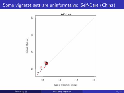
Some vignette sets are uninformative: Self-Care (China)

0.5 1.0 1.5 2.0

0.5

1.0

1.5

2.0

Self−Care


Est

imat

ed E

ntro

py

12

3

4

123124125134135145

234235245

345

12345121314

15

232425

3435

45

1234123512451345

2345


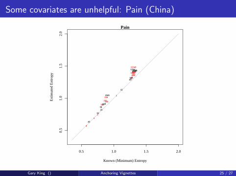
Some covariates are unhelpful: Pain (China)

0.5 1.0 1.5 2.0

0.5

1.0

1.5

2.0

Pain


Est

imat

ed E

ntro

py

1

2

3

4

123124125134135

145

234

235245345

12345

121314

15

2324

2534

35

45

1234123512451345

2345


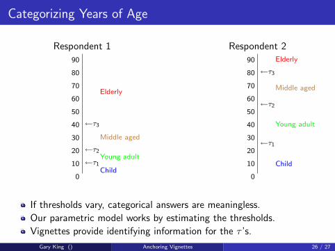
Categorizing Years of Age

Respondent 1

90

80

70

60Elderly

50

40 ←τ3

30 Middle aged

20 ←τ2Young adult

10 ←τ1Child

0

Respondent 2

90 Elderly

80 ←τ3

70 Middle aged

60

50←τ2

40 Young adult

30

20←τ1

10 Child

0

If thresholds vary, categorical answers are meaningless.

Our parametric model works by estimating the thresholds.

Vignettes provide identifying information for the τ ’s.


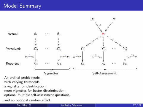
Model Summary

Xi

β

��666

6666

ηi

�� C�C�C�C

Actual: θ1

�� O�O�O

· · · θJ

�� O�O�O

µi

zz z:z:

z:z:

z:z:

��O�O�O

$$$d$d

$d$d

$d$d

Perceived: Z∗`1

V`

γ−→τ`

��

· · · Z∗`J

τ`

γ←−V`

��

Y ∗i1

τ

��Vi

γ−→τi

��

Y ∗i2

Vi

γ2−→τi2

��

· · · Y ∗iS

τiS

γS←−Vi

��Reported: z`1 9>>>>>>>>>>>=>>>>>>>>>>>; · · · z`J yi1 9>>>>>>>>>>>>>>>>>>>>>>>>=>>>>>>>>>>>>>>>>>>>>>>>>; yi2 · · · yiS

Vignettes Self-AssessmentAn ordinal probit model.with varying thresholds,a vignette for identification,more vignettes for better discrimination,optional multiple self-assessment questions,

and an optional random effect.


Self-Assessments v. Medical Tests

Self-Assessment:In the last 30 days, how much difficulty did [you/name] have in seeing andrecognizing a person you know across the road (i.e. from a distance ofabout 20 meters)? (A) none, (B) mild, (C) moderate, (D) severe, (E)extreme/cannot do

The Snellen Eye Chart Test:


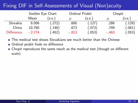
Fixing DIF in Self-Assessments of Visual (Non)acuity

Snellen Eye Chart Ordinal Probit ChopitMean (s.e.) µ (s.e.) µ (s.e.)

Slovakia 8.006 (.272) .660 (.127) .286 (.129)China 10.780 (.148) .673 (.073) .749 (.081)

Difference −2.774 (.452) −.013 (.053) −.463 (.053)

The medical test shows Slovakians see much better than the ChineseOrdinal probit finds no differenceChopit reproduces the same result as the medical test (though on differentscale)


Conclusions

Our approach can fix DIF, if response consistency and vignette equivalence hold —and the survey questions are good

Anchoring vignettes will not eliminate all DIF, but problems would have to occurat unrealistically extreme levels to make the unadjusted measures better than theadjusted ones.

Expense can be held down to a minimum by assigning each vignette to a smallersubsample. E.g., 4 vignettes asked for 1/4 of the sample each adds only onequestion/respondent.

If you think you have DIF-free questions, you now have the first real opportunity totest that hypothesis.

Whether or not you have DIF, vignettes can help us follow the usual survey adviceof making questions concrete. (Compare “say in government” with that questionplus the vignettes)

Writing vignettes aids in the clarification and discovery of additional domains ofthe concept of interest — even if you do not do a survey.

We do not provide a solution for other common survey problems: Questionwording, Accurate translation, Question order, Sampling design, Interview length,Social backgrounds of interviewer and respondent, etc.


For More Information

http://GKing.Harvard.edu/vign

Includes:

Academic papers

Anchoring vignette examples by researchers in many fields,

Frequently asked questions,

Videos

Conferences

Statistical software


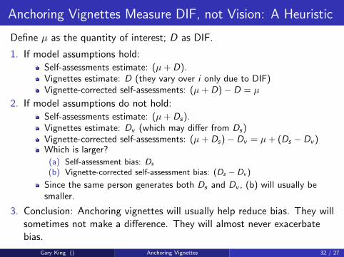
Anchoring Vignettes Measure DIF, not Vision: A Heuristic

Define µ as the quantity of interest; D as DIF.

1. If model assumptions hold:Self-assessments estimate: (µ + D).Vignettes estimate: D (they vary over i only due to DIF)Vignette-corrected self-assessments: (µ + D)− D = µ

2. If model assumptions do not hold:Self-assessments estimate: (µ + Ds).Vignettes estimate: Dv (which may differ from Ds)Vignette-corrected self-assessments: (µ + Ds)− Dv = µ + (Ds − Dv )Which is larger?

(a) Self-assessment bias: Ds

(b) Vignette-corrected self-assessment bias: (Ds − Dv )

Since the same person generates both Ds and Dv , (b) will usually besmaller.

3. Conclusion: Anchoring vignettes will usually help reduce bias. They willsometimes not make a difference. They will almost never exacerbatebias.


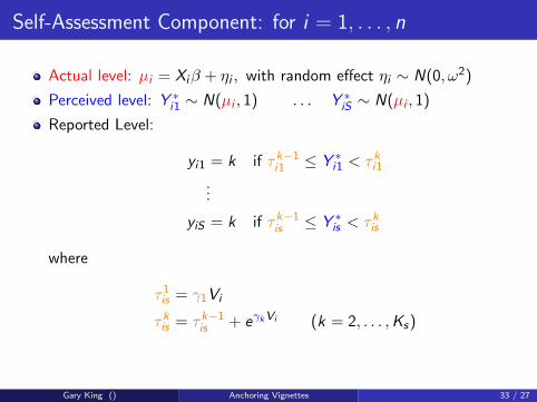
Self-Assessment Component: for i = 1, . . . , n

Actual level: µi = Xiβ + ηi , with random effect ηi ∼ N(0, ω2)

Perceived level: Y ∗i1 ∼ N(µi , 1) . . . Y ∗iS ∼ N(µi , 1)

Reported Level:

yi1 = k if τk−1i1 ≤ Y ∗i1 < τk

i1

...

yiS = k if τk−1is ≤ Y ∗is < τk

is

where

τ1is = γ1Vi

τkis = τk−1

is + eγkVi (k = 2, . . . ,Ks)


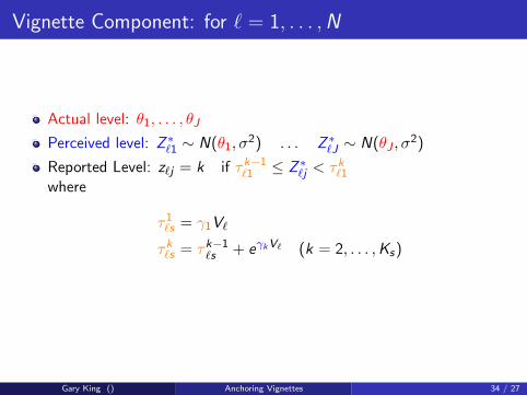
Vignette Component: for ` = 1, . . . , N

Actual level: θ1, . . . , θJ

Perceived level: Z ∗`1 ∼ N(θ1, σ2) . . . Z ∗`J ∼ N(θJ , σ

2)

Reported Level: z`j = k if τk−1`1 ≤ Z ∗`j < τk

`1

where

τ1`s = γ1V`

τk`s = τk−1

`s + eγkV` (k = 2, . . . ,Ks)


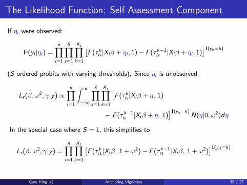
The Likelihood Function: Self-Assessment Component

If ηi were observed:

P(yi |ηi ) =n∏

i=1

S∏s=1

Ks∏k=1

[F (τ k

is |Xiβ + ηi , 1)− F (τ k−1is |Xiβ + ηi , 1)

]1(yis=k)

(S ordered probits with varying thresholds). Since ηi is unobserved,

Ls(β, ω2, γ|y) ∝n∏

i=1

∫ ∞

−∞

S∏s=1

Ks∏k=1

[F (τ k

is |Xiβ + η, 1)

− F (τ k−1is |Xiβ + η, 1)

]1(yis=k)N(η|0, ω2)dη

In the special case where S = 1, this simplifies to

Ls(β, ω2, γ|y) =n∏

i=1

K1∏k=1

[F (τ k

i1|Xiβ, 1 + ω2)− F (τ k−1i1 |Xiβ, 1 + ω2)

]1(yi1=k)


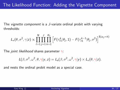
The Likelihood Function: Adding the Vignette Component

The vignette component is a J-variate ordinal probit with varyingthresholds:

Lv (θ, σ2, γ|z) ∝N∏

`=1

J∏j=1

K1∏k=1

[F (τk

`1|θj , 1)− F (τk−1`1 |θj , σ

2)]1(z`j=k)

The joint likelihood shares parameter γ:

L(β, σ2, ω2, θ, γ|y , z) = Ls(β, σ2, ω2, γ|y)× Lv (θ, γ|z).

and nests the ordinal probit model as a special case.


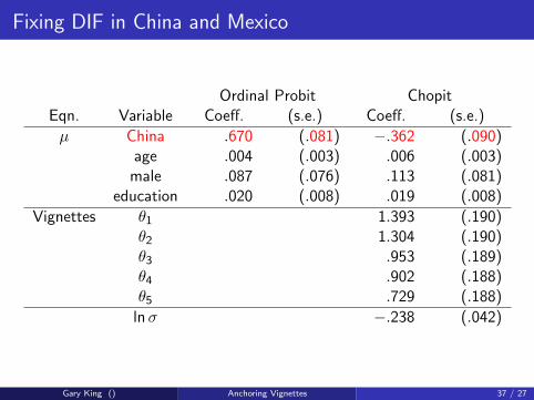
Fixing DIF in China and Mexico

Ordinal Probit ChopitEqn. Variable Coeff. (s.e.) Coeff. (s.e.)

µ China .670 (.081) −.362 (.090)age .004 (.003) .006 (.003)male .087 (.076) .113 (.081)

education .020 (.008) .019 (.008)

Vignettes θ1 1.393 (.190)θ2 1.304 (.190)θ3 .953 (.189)θ4 .902 (.188)θ5 .729 (.188)

lnσ −.238 (.042)


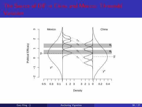
The Source of DIF in China and Mexico: ThresholdVariation

Density

Pol

itica

l Effi

cacy

−2

−1

01

23

0.5 0.3 0.1 1 2 3 3 2 1 0 0.2 0.4

θ1

θ5

Mexico China

y*y*

τ1

τ2

τ3

τ4

µµ


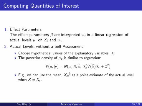
Computing Quantities of Interest

1. Effect ParametersThe effect parameters β are interpreted as in a linear regression ofactual levels µi on Xi and ηi .

2. Actual Levels, without a Self-Assessment

Choose hypothetical values of the explanatory variables, Xc

The posterior density of µc is similar to regression:

P(µc |y) = N(µc |Xc β̂, X ′c V̂ (β̂)Xc + ω̂2)

E.g., we can use the mean, Xc β̂ as a point estimate of the actual levelwhen X = Xc .


Estimating Actual Levels, with a Self-Assessment

1. If we know yi , why not use it?

2. For example,

Suppose John and Esmeralda have the same X valuesBy Method 1, they give the same inferences: P(µJ |y) = P(µE |y).Suppose John’s yJ value is near µ̂J and but Esmeralda’s is far away.

Under Method 1, nothing’s new. Predictions are unchanged.Intuitively, John is average and Esmeralda is an outlierWe should adjust our prediction from µ̂E toward yE .

So the new method takes roughly the weighted average of the modelprediction µ̂E and the observed yE , with weights determined by the howgood a prediction it is.


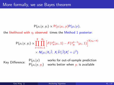
More formally, we use Bayes theorem

P(µi |y , yi ) ∝ P(yi |µi , y)P(µi |y),

the likelihood with ηi observed times the Method 1 posterior:

P(µi |y , yi ) ∝S∏

s=1

Ks∏k=1

[F (τ̂k

is |µi , 1)− F (τ̂k−1is |µi , 1)

]1(yis=k)

× N(µi |Xi β̂, Xi V̂ (β̂)X ′i + ω̂2)

Key Difference:P(µi |y) works for out-of-sample predictionP(µi |y , yi ) works better when yi is available


Unconditional Posterior

−2 −1 0 1 2

0.0

1.0

2.0

3.0

µc

Den

sity

Truth ChopitOrderedProbit

Unconditional posterior for a hypothetical 65-year-old respondent incountry 1, based on one simulated data set.


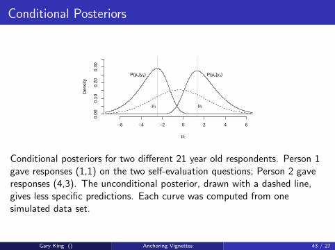
Conditional Posteriors

−6 −4 −2 0 2 4 6

0.00

0.10

0.20

0.30

µc

Den

sity

µ1 µ2

P(µ1|y1) P(µ2|y2)

Conditional posteriors for two different 21 year old respondents. Person 1gave responses (1,1) on the two self-evaluation questions; Person 2 gaveresponses (4,3). The unconditional posterior, drawn with a dashed line,gives less specific predictions. Each curve was computed from onesimulated data set.


Anchoring Vignettes for Interpersonally Incomparable ...

Documents