Anatomical limits on interaural time differences: an ...

ORIGINAL RESEARCH ARTICLEpublished: 28 February 2014

doi: 10.3389/fnins.2014.00034

Anatomical limits on interaural time differences: anecological perspectiveWilliam M. Hartmann* and Eric J. Macaulay

Psychoacoustics Laboratory, Department of Physics and Astronomy, Michigan State University, East Lansing, MI, USA

Edited by:

Guillaume Andeol, Institut deRecherche Biomédicale desArmées, France

Reviewed by:

Dan Tollin, University of ColoradoSchool of Medicine, USAFrederick J. Gallun, Portland VAMedical Center, USA

*Correspondence:

William M. Hartmann, Departmentof Physics and Astronomy, MichiganState University, 567 Wilson Rd.,East Lansing, MI 48824, USAe-mail: [email protected]

Human listeners, and other animals too, use interaural time differences (ITD) to localizesounds. If the sounds are pure tones, a simple frequency factor relates the ITD tothe interaural phase difference (IPD), for which there are known iso-IPD boundaries,90◦, 180◦ . . . defining regions of spatial perception. In this article, iso-IPD boundariesfor humans are translated into azimuths using a spherical head model (SHM), and thecalculations are checked by free-field measurements. The translated boundaries providequantitative tests of an ecological interpretation for the dramatic onset of ITD insensitivityat high frequencies. According to this interpretation, the insensitivity serves as a defenseagainst misinformation and can be attributed to limits on binaural processing in thebrainstem. Calculations show that the ecological explanation passes the tests only ifthe binaural brainstem properties evolved or developed consistent with heads that are50% smaller than current adult heads. Measurements on more realistic head shapesrelax that requirement only slightly. The problem posed by the discrepancy between thecurrent head size and a smaller, ideal head size was apparently solved by the evolutionor development of central processes that discount large IPDs in favor of interaural leveldifferences. The latter become more important with increasing head size.

Keywords: brainstem, evolution, binaural, sound localization, interaural time difference, spherical head model,

rotation-azimuth transform

1. INTRODUCTIONMore than 100 years ago, Lord Rayleigh pointed out that humanlisteners can make use of interaural time differences (ITD) tolocalize pure tones (Strutt, 1907). An example is illustrated bythe functions in Figure 1, which represent the pressures at thetwo ears for a 1000-Hz tone. Here, the source of the tone is onthe listener’s right side so that the waveform in the right ear (red)starts before the waveform in the left (blue and dashed). As shownin region A, the ongoing wave in the right ear continues to leadthe ongoing wave in the left. For instance, the positive-going zerocrossing at time to in the left ear is preceded by a similar crossingin the right.

1.1. THE INTERAURAL PHASE PROBLEMRayleigh was quick to point out that there are practical limitsto the utility of the ITD. When the azimuth increases enoughthat the interaural phase difference (IPD) becomes equal to 180◦,the ongoing information from the ITD becomes totally ambigu-ous. As the azimuth increases further, and the IPD exceeds 180◦(regions C and D), the ITD points to images with azimuths oppo-site to the actual source azimuth. Headphone experiments byBernstein and Trahiotis (1985) have revealed just this kind ofambiguity. Thus, there is a 180◦ IPD limit on useful ITD cues.Region D is especially misleading—even dangerous. Although thesource continues to be on the listener’s right, the ongoing wave-form indicates that the source is on the left—just as surely as itpointed to a source on the right in region A. In free-field listen-ing, this misleading ongoing information actually dominates the(correct) onset information (Hartmann and Rakerd, 1989).

Sayers (1964) reported experiments indicating another IPDboundary of interest. As the ITD increases such that the IPDexceeds about 90◦ (region B), further increases in ITD cause theimage to move back toward the midline. Also, in region B listen-ers sometimes lateralize images on the wrong side of the head.Yost (1981) similarly found frequent wrong-side lateralization inregion B, and Elpern and Naughton (1964) showed that the max-imum sensation of lateralization occurs for IPD = 90◦. Thus,there is a 90◦ IPD limit on useful directional information fromchanges in the ITD, and the regions of ITD information are logi-cally represented by IPD boundaries separated by 90◦ as shown inFigure 1.

Region E shows a confusion of yet another sort. Here, theongoing waveforms are identical to those in region A, but theITD in region E is larger by a full period of the tone (1000 μs).The same ongoing waveform corresponds to two different ITDs,indicating two different characteristic delays of the same sign,potentially associated with two different locations on the sameside of the head.

It has been proposed that the IPD confusions noted here havebeen ameliorated by a binaural system that becomes insensitiveto ITDs at high frequency. This idea will be called the “ecologicalinterpretation,” and the rest of this article will study its plausibilityand possible modifications to it.

1.2. TRANSFORMATIONSBecause the IPD is the product of the ITD and the frequencyof the tone, the IPD boundaries of Figure 1 can be translatedto ITD and frequency, as shown in Figure 2. These boundaries

www.frontiersin.org February 2014 | Volume 8 | Article 34 | 1

Hartmann and Macaulay Limits for interaural time differences

will be called “iso-IPD contours” or simply “IPD contours” or“IPD boundaries.” The dashed horizontal line (HW) indicatesthe largest ITD that can be caused by the typical human headfor sound sources in free field, sometimes called the Hornbostel–Wertheimer constant (von Hornbostel and Wertheimer, 1920).Figure 2 shows it as the low-frequency limit of the head diffrac-tion formula ITD = (3a/v) sin(90◦) = 763μs. Here a (8.75 cm)

A

C

D

E

B

FIGURE 1 | Tones in the right ear (red) and left ear (blue and dashed) as

functions of time and with particular interaural phase differences (IPD)

as indicated on the vertical axis to illustrate different regions of IPD.

The boundaries between regions, separated by 90◦, are logically andperceptually important in sound localization.

A B C D E

FIGURE 2 | Transformation of the iso-IPD boundaries in Figure 1 to a

scale of frequency and interaural time difference (ITD). HW indicatesthe largest possible ITD for the average human head in free field.

is the radius of the typical human head (Hartley and Fry, 1921;Algazi et al., 2001), and v (34,400 cm/s), is the speed of sound inroom-temperature air.

Figure 2 shows that the iso-IPD contours, such as the 90◦ or180◦ boundaries, are not important if the ITD is small or thefrequency is low. Small ITDs occur in the real world when theazimuth of the source is small. Large ITDs, and large IPDs, occurwhen the source is off to the side of the listener. A representationin terms of source azimuth can be obtained by transforming theITD axis in Figure 2 to a scale of source azimuth, as shown inFigure 3.

2. SPHERICAL HEAD MODELThe shaded regions in Figure 3 are transformations to anazimuthal scale using a spherical head model (SHM). The iso-IPD contours separating the regions in Figure 2 have become thinregions corresponding to different locations of the ears on thehead.

2.1. SPHERICAL HEAD CALCULATIONSThe calculations for Figure 3 were based on an exact mathe-matical treatment of the scattering of waves by a rigid sphere.Solutions to this scattering problem for plane wave incidence(infinite source distance) go back as far as Rayleigh (1896).A modern solution, which is a series of Legendre polynomialswith frequency-dependent, complex spherical functions as coef-ficients, was given by Rschevkin (1963) and applied to interauraldifferences for a spherical head by Kuhn (1977). The spheri-cal head calculation was generalized to finite source distanceby Rabinowitz et al. (1993) and Duda and Martens (1998). Inthe limit of infinite source distance, the finite-distance solution

A B C D

FIGURE 3 | Transforming the ITD axis in Figure 2 to an azimuthal axis

using the spherical head diffraction model. The blue shaded regions arebounded by ear angles of 90◦ (solid blue line) and 110◦. The green shadedregion similarly shows the Woodworth model. The red dashed curves showthe low-frequency limit of the spherical head model for IPDs of 90◦ and180◦.

Frontiers in Neuroscience | Auditory Cognitive Neuroscience February 2014 | Volume 8 | Article 34 | 2

Hartmann and Macaulay Limits for interaural time differences

reduces to Kuhn’s result. Our Figure 3 used the finite-distancesolution with a source distance of 2 m to match experiment.However, there is actually very little difference between ITDscomputed for a source at 2 m and a source at infinity. (The inter-aural level difference is much more sensitive to source distance.)The spherical head solution captures the important frequencydependence of the ITD that is also characteristic of human heads.The frequency dependence of the ITD for different azimuths, asplotted by Constan and Hartmann (2003) (their Figure 1), showsa significant drop in ITD between 400 and 2000 Hz.

The low-frequency limit, (3a/v) sin(θ) generally underesti-mates the ITD at low frequency. For instance, Kuhn (1977)found that in order to match low-frequency KEMAR ITDs, it wasnecessary to increase the head radius from a = 8.75 to 9.3 cm.Kuhn tentatively attributed the apparent extra size to the pin-nae, which would be indistinguishable from the bulk of the headwhen viewed with wavelengths corresponding to low frequen-cies. Fortunately, all the frequencies of interest in the currentarticle are greater than 600 Hz, and in this range, the SHMITD agrees better with measurements on human listeners. Thehigh-frequency limit of the SHM is the creeping wave solutionknown as the Woodworth model (Woodworth, 1938). In thislimit ITDs are smaller than in the low-frequency limit, with thedecrease depending on the azimuth. For small azimuths, the high-frequency limiting ITD is 33% smaller than the low-frequencylimit. At the other extreme, an azimuth of 90◦, the high-frequencyITD is only 14% smaller.

The shaded contours in Figure 3 arise from a range of assump-tions about the angle of the listener’s ears with respect to theforward direction. The boundaries indicated with solid blue linescorrespond to an ear angle of 90◦; the other edges of the shadedregions correspond to 110◦. Thus, the contours are centered onan ear angle of 100◦, as suggested by Blauert (1997) and used byDuda and Martens (1998) and by Treeby et al. (2007). For com-parison, we note that Hartley and Fry (1921) suggested that thehuman ear is 97.5◦.

The red, dashed lines represent the low-frequency (f ) limitof the azimuth (�) for a spherical head with radius a: � =arcsin[v/(6fa)] for the 180◦ IPD limit and � = arcsin[v/(12fa)]for the 90◦ IPD limit.

As expected, the low-frequency limit agrees with the exact for-mula for a 90◦ ear angle near 400 Hz and departs from the exactformula as the frequency increases. The green, shaded region athigh frequency shows the 360◦ IPD contour from the Woodworthmodel, which is only valid at high frequency. The calculationsfor ear angles between 90◦ and 110◦ were made using formulasfor the Woodworth model from Aaronson and Hartmann (2014).This latter article shows that unless the frequency is very high,the Woodworth formula underestimates the ITD. That is why,for every frequency, an especially large azimuth is required toproduce a given IPD—in this case, an IPD of 360◦.

2.2. SPHERICAL HEAD ARRAY MEASUREMENTSThe spherical head calculations in Figure 3 were tested againstmeasurements of frequency and azimuth that targeted IPDs ofinterest. Measurements were made in an anechoic room (7.7 ×6.4 × 3.6 m) (IAC 107840) using an array of 13 loudspeaker

sources (Minimus 3.5) spaced by 7.5◦ and located 2 m away froma binaural receiver. The array was a single quadrant (0–90◦) tothe right of the receiver. The receiver was a rigid spherical shell(Shapemaster, Ogden, IL) with a radius of 8.75 cm made of 6-mmPETG (glycol-modified polyethylene terephthalate) and mountedon a microphone stand 117 cm off the wire grid floor, the sameheight as the array sources. The forward direction of the spherewas defined by a laser beam through the center of the sphere.Two small holes were drilled at 90◦ from the forward direc-tion to accommodate the ends of the probe tubes (0.95 mmO.D.) of Etymotic ER-7c probe microphones. (Etymotic Research,Elkgrove Village, IL). Therefore, the simulated ear angles were90◦. Signals from the microphones were first amplified with theassociated probe-tube-compensating Etymotic preamplifier, andthen given another 40 dB of gain before conversion to digital formby a DD1 two-channel 16-bit analog-to-digital converter (Tucker-Davis Technologies, Alachua, FL). Because the frequency of thesignal was exactly known, it was possible to use matched filter-ing to process half-second samples of the digitized signals and toextract precise IPDs.

Estimates for the target IPD boundaries of 90◦, 180◦, 270◦,and 360◦ are shown in Figure 4. They were determined by set-ting the frequency to successive values and measuring IPDs for the13 sources. Then, source azimuths for the target IPD boundarieswere interpolated from the measured IPDs. The interpolationprocedure required the assumption that the IPD-azimuth rela-tionship was smooth and locally linear. Figure 4 shows that theinterpolated azimuths agree reasonably well with the solid lines atthe tops of the shaded regions, as expected for a 90◦ ear angle.

2.3. SPHERICAL HEAD ROTATION MEASUREMENTSBecause of our concern with the interpolated array measurementsover 7.5◦ and with inadvertent scattering from the array structure

A B C D E

FIGURE 4 | Measured values of frequency and azimuth that lead to

IPDs of 90◦, 180◦, 270◦, and 360◦ (diamonds, circles, squares, triangles,

respectively) for a perfect sphere. Values were interpolated frommeasurements using a source array in one quadrant.

www.frontiersin.org February 2014 | Volume 8 | Article 34 | 3

Hartmann and Macaulay Limits for interaural time differences

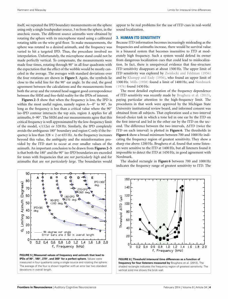
itself, we repeated the IPD boundary measurements on the sphereusing only a single loudspeaker source, 3 m from the sphere, in theanechoic room. The different source azimuths were obtained byrotating the sphere with its microphone stand using a calibratedrotating table on the wire grid floor. To make measurements, thesphere was rotated to a desired azimuth, and the frequency wasvaried to hit a targeted IPD. Thus, the procedure involved nointerpolation. Unfortunately, the microphone stand could not bemade perfectly vertical. To compensate, the measurements weremade four times, rotating through 90◦ in all four quadrants withthe expectation that the effect of the wobble would be mostly can-celed in the average. The averages with standard deviations overthe four rotations are shown in Figure 5. Again, the symbols lieclose to the solid line for the 90◦ ear angle. In the end, the goodagreement between the calculations and the measurements fromboth the array and the rotated head suggest good correspondencebetween the SHM and free-field reality for the IPDs of interest.

Figures 2–5 show that when the frequency is low, the IPD iswithin the most useful region, namely region A—0◦ to 90◦. Solong as the frequency is less than a critical value where the 90◦iso-IPD contour intersects the top axis, region A applies for allazimuths, 0–90◦. The SHM and our measurements agree that thiscritical frequency is well approximated by the low-frequency limitof the model, v/(12a) or 328 Hz. Similarly, the IPD completelyavoids the ambiguous 180◦ boundary and region C only if the fre-quency is less than 328 × 2 or 655 Hz. As the frequency increasesbeyond this value, the ambiguity and the misinformation pro-vided by the ITD start to occur at ever smaller values of theazimuth. An important conclusion to be drawn from Figures 2–5is that both the 180◦ and the 90◦ iso-IPD boundaries are exceededfor tones with frequencies that are not particularly high and forazimuths that are not particularly large. The boundaries would

A B C D E

FIGURE 5 | Measured values of frequency and azimuth that lead to

IPDs of 90◦, 180◦, 270◦, and 360◦ for a perfect sphere. Values weremeasured in four quadrants using a single source and rotating the sphere.The average of the four is shown together with an error bar two standarddeviations in overall length.

appear to be real problems for the use of ITD cues in real-worldsound localization.

3. HUMAN ITD SENSITIVITYBecause ITD information becomes increasingly misleading as thefrequencies and azimuths increase, there would be survival valuein a binaural system that becomes insensitive to ITD at mod-erately high frequency. Such a system would defend its ownerfrom dangerous localization cues that could lead to mislocaliza-tion. In fact, there is unequivocal evidence that fine-structureITD sensitivity disappears at about 1500 Hz. The upper limit ofITD sensitivity was explored by Zwislocki and Feldman (1956)and by Klumpp and Eady (1956), who found an upper limit of1300 Hz. Mills (1958) found a limit of 1400 Hz, and Nordmark(1976) found 1430 Hz.

The most detailed exploration of the frequency dependenceof ITD sensitivity was recently made by Brughera et al. (2013),paying particular attention to the high-frequency limit. Theprocedures in that work were approved by the Michigan StateUniversity institutional review board, and informed consent wasobtained from all subjects. That exploration used a two-intervalforced-choice task in which a tone led in one ear by the ITD onthe first interval and led in the other ear by the ITD on the sec-ond. The difference between the two intervals, �ITD (twice theITD on each interval) is plotted in Figure 6. The thresholds inFigure 6 show a broad minimum between 700 and 1000 Hz indi-cating the frequency region of greatest sensitivity. They show asharp rise above 1200 Hz. Brughera et al. found that some listen-ers were sensitive to the ITD at 1400 Hz, but all listeners found itimpossible to detect the ITD at 1450 Hz, in good agreement withNordmark.

The shaded rectangle in Figure 6 between 700 and 1000 Hzindicates the frequency range of greatest sensitivity to ITD. The

FIGURE 6 | Threshold interaural time differences as a function of

frequency for four listeners measured by Brughera et al. (2013). Theshaded rectangle indicates the frequency region of greatest sensitivity. Thevertical solid line shows the brick wall.

Frontiers in Neuroscience | Auditory Cognitive Neuroscience February 2014 | Volume 8 | Article 34 | 4

Hartmann and Macaulay Limits for interaural time differences

vertical line in Figure 6 at 1450 Hz indicates the upper limit.Because we are unaware of any experiment indicating ITD sen-sitivity for a tone with a frequency greater than 1450 Hz, the restof this article will refer to the boundary at 1450 Hz as the “brickwall.” It is striking that the frequency difference between the top ofthe region of greatest sensitivity and the brick wall is considerablyless than an octave. It is an unusually sharp transition.

The loss of ITD sensitivity for sine tones above 1450 Hz is con-sistent with other binaural phenomena, such as binaural beats,which indicate a loss of interaural phase sensitivity near thisfrequency (Perrott and Nelson, 1969). Although the binauralmasking level difference (MLD) is a more complicated effect,there is evidence of a similar limit in a dozen experiments citedby Durlach (1972), where the MLD as a function of frequencyshows a discontinuity in slope near 1500 Hz (Durlach Figure 4).

The loss of phase sensitivity at the brick wall appears to bespecifically a binaural phenomenon. There is good reason tobelieve that phase locking is maintained in the human auditorysystem for considerably higher frequencies. A low estimate forthe loss of phase locking (between 2 and 3 kHz) comes from mis-tuned harmonic detection experiments (Hartmann et al., 1990).A high estimate (8 kHz) comes from frequency difference limenexperiments (Moore and Ernst, 2012). Intermediate estimates(4–5 kHz) come from musical pitch experiments (e.g., Oxenhamet al., 2011) or from assuming that phase locking in humans issimilar to the auditory nerve of cat (Johnson, 1980). Apparentlythere is an especially low limit for the human binaural system.But although the lowpass character must follow the initial stageof binaural interaction, it is not certain where it originates. Theneural modeling by Brughera et al. (2013), based on cat and gerbilphysiology, identified the superior olive complex in the brainstemas the origin of the low limit. Whether the limit occurs in thesuperior olive or in the inferior colliculus, it is not unreasonableto focus on the brainstem and to conjecture that the limit repre-sents an evolutionary adaptation of the brainstem to ITD valuesof negative utility as seen in Figures 2–5.

4. THE ECOLOGICAL INTERPRETATIONAn ecological interpretation for the high-frequency limits ofITD sensitivity has often been proposed. Rayleigh (Strutt, 1907)argued that it was unlikely that listeners could localize soundsbased only on ITD when the frequency was much above 512 Hzbecause the maximum delay across the head (about 800 μs)would lead to an IPD close to 180◦. In 1909, Rayleigh (Strutt,1909) also remarked on the 90◦ IPD boundary, leading to aneven lower estimate for the maximum frequency for useable ITD.Yost and Hafter (1987) noted that delaying a 1666-Hz tone bya head width would be equivalent to no delay at all (region E).The 2005 review of binaural hearing by Stern et al. (2005) sim-ilarly suggested that the upper limit of ITD utility should be setby the size of the head. Moore’s introduction to human hearing(1997) also noted the correspondence between the ambiguity ofthe ITD cue and the distance between the ears. Taking a some-what different direction, Blauert (1997) argued that the headsize establishes an upper limit of about 630 μs on useful ITDs.Schnupp et al. (2011) argued similarly, applying the same princi-ple to all animals. Carlile (1996) noted that the only unambiguous

tones are those with wavelength less than twice the head radius.Calculations by Harper and McAlpine (2004) showed that theoptimum array for coding of cross-correlation in IPD-frequencyspace is mainly a function of an animal’s head size.

As shown in Figures 2–5, the azimuths for the boundariesIPD = 90◦ and 180◦ are rapidly varying functions of frequencyin the large azimuth regime. As shown in Figure 6, the ITD sen-sitivity also has a rapid frequency dependence. According to theecological interpretation (EI), these regions of changing sensi-tivity ought to be sensibly related. Figure 7 repeats the sphericalhead regions from Figure 3, and also repeats the region of greatestITD sensitivity and the brick wall from Figure 6. Figure 7 showsthat the relationship is far from sensible.

As shown by the dotted lines in Figure 7, for the 180◦ bound-ary, the EI would assert that the binaural system has becomeinsensitive to 1450-Hz tones because the IPD exceeds 180◦, lead-ing to wrong-sided images, whenever the azimuth is greater than33◦. By contrast, the binaural system has remained highly sensi-tive to 1000-Hz tones because they are more reliable. They lead towrong-sided images only when the azimuth is greater than 45◦.The problem with this picture is that the difference of only 12◦of azimuth is hardly adequate motivation for a system to developsuch a sharply tuned frequency response as the human binauralITD system evidently has.

The corresponding analysis for the 90◦ iso-IPD contour (notshown in the figure) is even more disappointing. According tothe EI, the binaural system rejects ITD information from a 1450-Hz tone because this tone leads to perceived images that movein directions opposite to reality when the azimuth is greater than14◦. By contrast, the binaural system maintains sensitivity to ITDinformation at 1000 Hz because it leads to misleading directionalinformation only when the azimuth is greater than 24◦. Again, thedifference of only 10◦ seems to be a poor reason to evolve an ITD

A B C D E

FIGURE 7 | Sensitivity regions from Figure 6 together with model

boundaries for the IPD regions from Figure 3. The dotted lines refer tothe argument in the text against the ecological interpretation givenpresent-day human head sizes.

www.frontiersin.org February 2014 | Volume 8 | Article 34 | 5

Hartmann and Macaulay Limits for interaural time differences

with a sharp frequency cutoff. Given the poor correspondencebetween the IPD boundaries and the limits of ITD sensitivity, oneis tempted to abandon the ecological interpretation, at least in thequantitative detail presented here. Perhaps evolutionary pressuresare actually responsible for the anomalously low cutoff frequencyof ITD sensitivity, but then evolution stopped too soon and didn’tget the cutoff quite low enough.

There is an alternative ecological theory, however, that leadsto quantitatively good correspondence. The theory assumes thatwhile the brainstem was evolving, and the medial superior oliveand projections to it were developing, the head size was consider-ably smaller than the current human head. Figure 8 is a repeat ofFigure 7 except that it makes the small-head hypothesis, assum-ing that the head is 50% smaller than our present-day humanheads—a factor of 2 in diameter.

In Figure 8 the upper limit of ITD sensitivity at 1450 Hz essen-tially eliminates the confusing ITDs in regions C, D, and E fromcontributing to sound localization. Only tones with an IPD lessthan the 180◦ iso-IPD contour can contribute. In another bene-fit, the most sensitive region between 700 and 1000 Hz extends tosource azimuths as large as 60◦. For the 90◦ iso-IPD contour, ITDinformation for 1450-Hz tones would be rejected because it leadsto an incorrect sense of motion when the azimuth is greater than27◦. The confusing 90◦ iso-IPD contour does not enter the regionof greatest ITD sensitivity until the azimuth has reached 40◦ (upfrom 23◦). Therefore, a binaural system that developed to opti-mize ITD coding for a head diameter that is half as large appearsto make sense acoustically. It makes some sense in evolutionaryterms too because the brainstem is old brain, whereas the headexpanded over very recent times to accommodate the neocortex.

A factor of two in diameter, however, may be extreme. Overthe past 3.2 million years the brain size has expanded by a factorof 3 (Lynn, 1990). The cube root of 3 is 1.44 suggesting a headdiameter that was 30% smaller than present day. Making the head

A B C D E

FIGURE 8 | Same as Figure 7 for a head diameter that is half as large

as present-day human heads.

diameter 30% smaller (not shown in the figures) confers someadvantages. Then the brick wall at 1450 Hz totally eliminates themost dangerous region, region D, for all azimuths.

The small-head hypothesis carries with it the assumption thatthe binaural properties of the brainstem have not greatly changedsince the origin of homo with rapidly growing heads. Thatassumption can certainly be challenged because there is evidencethat the binaural system changes—even in a single individual,even over a brief time. Evidence for changeable binaural process-ing is found in studies of development and plasticity. Experimentsby Shinn-Cunningham et al. (1998), in which human auditoryspatial maps were altered by feedback, or experiments by Hofmanet al. (1998), where maps were altered by plugging one ear, showat least partial adaptation to new conditions. It is possible thoughthat short-term accommodations such as these are entirely theresult of cortical plasticity, revealing nothing about the brainstem.Concerning the brainstem itself, auditory brainstem response(ABR) experiments, as described in the review by Tzounopoulosand Kraus (2009), indicate plasticity in the brainstem that is bothsynaptic and intrinsic. The intrinsic plasticity shows changes at afundamental biochemical level—a likely origin for the ITD brickwall. If brainstem plasticity appears on the time scale of a briefexperiment or the development of a single individual, it seemsunlikely that the binaural system would be resistant to ecologicalpressures for a few million years.

In contrast to the plasticity argument above, we conjec-ture that the binaural system, once adjusted for the ITDsavailable with small heads, did not change over evolution-ary times because evolution found an alternative way to solvethe problem of misleading ITDs, namely by using interaurallevel differences (ILD), which grew to be substantial as thehead grew.

Calculations within the SHM show that the ILD is adequateto solve the problem in regions B, C, and D of Figure 7. Alongthe 90◦ iso-IPD contour (limit of region B), the ILD is greaterthan 2 dB except for the lowest frequencies, below 500 Hz. Even atthe lowest frequencies the ILD is greater than 2 dB if the sourceis closer than 2 m. Along the 180◦ iso-IPD contour (limit ofregion C), the ILD is always greater than 3.5 dB and usually ismuch larger. ILDs of these magnitudes are adequate for humanlisteners to localize on the correct side of the head especiallybecause the ITD cues are weak in these regions. Region D issomewhat more problematical. There, misleading ITD cues canbe strong, and the correct ILDs along the 270◦ iso-IPD con-tour from 1100 to 1500 Hz are only slightly larger than alongthe 180◦ contour, partly because the relevant azimuths becomelarge enough to involve the acoustical bright spot (Macaulay et al.,2010). Although region D, with strong, but wrong, ITD cues,represents more of a problem than region C, it is possible forthe misleading ITD cues in both regions to be overcome at ahigher level by a process that discounts ITD cues by contraveningILD cues.

The ILD does not solve the confusion problem in region E,where both the ITD and the ILD point in the same direction, andthe ITD points to a secondary azimuth. However, Figure 7 (cur-rent head size) shows that region E is perfectly eliminated by thebrick wall at 1450 Hz.

Frontiers in Neuroscience | Auditory Cognitive Neuroscience February 2014 | Volume 8 | Article 34 | 6

Hartmann and Macaulay Limits for interaural time differences

5. KEMAR MEASUREMENTSThe experimental approach to the ecological interpretation usingthe spherical head (section 2) was consistent with historicalapproaches from the time of Rayleigh to the present. It proba-bly applies to human heads better than to the other mammalsthat are frequently studied. It is possible, however, that the prop-erties of real human heads might differ from the (SHM) in someimportant way with consequences for the theory. To obtain mea-surements of the IPD boundaries that are more realistic, we used aKEMAR manikin (large ears). As for the perfect sphere, we madetwo different measurements in the anechoic room, one with the2-m array of 13 sources and the other with a rotating receiver anda single source. The sources were again at ear height.

Tones of fixed frequency were reproduced by the sources, andwere recorded by the Etymotic ER-11 microphones within theKEMAR head and associated electronics. The recordings wereagain processed by matched filtering to obtain IPDs.

5.1. ARRAY MEASUREMENTSThe source azimuths leading to 90◦ and 180◦ IPDs were deter-mined by linear interpolation within the 2-m array for a seriesof tone frequencies. The results are shown in Figure 9 by circlesand diamonds, which follow a smooth descending pattern exceptfor prominent bumps near 1.3 kHz. We noted that a frequency of1.3 kHz is close to the brick wall.

We suspected that the bumps were due to reflections fromthe manikin torso, and to test that idea we separated the headfrom the torso and mounted it on a microphone stand. However,the bumps persisted—somewhat changed in shape but at aboutthe same frequencies. We next questioned the microphone sys-tem intrinsic to the KEMAR, and as a check on that system,we replaced it by probe microphones in the KEMAR ear canals

A B C D E

FIGURE 9 | Measured values of frequency and azimuth that lead to

IPDs of 90◦ and 180◦ for a KEMAR manikin. Values were interpolatedfrom measurements using a source array in one quadrant to the right of themanikin.

(Etymotic ER-7c with associated electronics). The measurementswith the alternative system almost perfectly reproduced thosemade with the KEMAR microphone system, including the bumps.

Because the bumps in the iso-IPD contours were observedin all our KEMAR head configurations and not observed in thearray measurements using the perfect sphere, we tentatively con-cluded that the bumps near 1.3 kHz were caused by diffractionby the KEMAR head itself. However, the interpolated measure-ments from the array make assumptions about the smoothnessof the contours, and those assumptions might not hold for acomplicated head structure.

5.2. ROTATING KEMAR MEASUREMENTSTo check the measurements made with the array, we used a singleloudspeaker 3 m away from the KEMAR, as for the rotated spheremeasurements. We obtained different source azimuths by rotatingthe KEMAR with its mounting pole as an axis. However, unlikethe sphere, the axis of rotation did not pass through the center ofthe head (COH). To relate angles of rotation to source azimuths,we developed the mathematics in Appendix, which solves theproblem in principle. The KEMAR has a “+” sign on the top of itscranium and we took that point to be the COH for all measure-ments. The perpendicular distance from that point to the axis ofrotation is 2 cm. As shown in the Appendix, the rotation-azimuthtransformation depends on the ratio of this distance to the sourcedistance, in this case a ratio of 2/300. With this value, the formulain the Appendix leads to an angular discrepancy of 0.5◦, an errorthat can be ignored for our purposes.

Figure 10 shows the iso-IPD contours with mean and standarddeviation measured across the two frontal quadrants. Figure 11shows the same for the two back quadrants. Although the details

A B C D E

FIGURE 10 | Measured values of frequency and azimuth for IPDs of 90◦,

180◦, 270◦, and 360◦ for a rotated KEMAR manikin. Values weremeasured in left and right quadrants in front of the head using a singlesource. The average of the two quadrants is shown together with an errorbar two standard deviations in overall length. Long error bars indicateregions of non-monotonic IPD.

www.frontiersin.org February 2014 | Volume 8 | Article 34 | 7

Hartmann and Macaulay Limits for interaural time differences

A B C D E

FIGURE 11 | Measured values of frequency and azimuth for IPDs of 90◦,

180◦, 270◦, and 360◦ for a rotated KEMAR manikin. Values weremeasured in left and right quadrants in back of the head using a singlesource. The average of the two quadrants is shown together with an errorbar two standard deviations in overall length. Long error bars indicateregions of non-monotonic IPD.

of the plots are not identical to Figure 9, the overall shape isthe same, and the bumps for the 90◦ and 180◦ iso-IPD bound-aries occur at the same frequencies. Figures 10, 11 also show thatthe bumps occur at higher frequencies for the higher iso-IPDboundaries. The iso-IPD boundary measurements are similarfor sources in front of the head (Figure 10) and sources behindthe head (Figure 11). Some of the error bars seem rather long,especially as the frequency increases. However, these error barsdon’t represent actual errors. Instead, they represent regions offrequency and azimuth where the IPDs are not monotonic func-tions and oscillate around the boundary value. These badly-actingregions became evident as we rotated the head and varied the fre-quency. It also became evident that the disagreements betweenFigures 9 and 10 owe much to the failure of the assumptionsof smoothness and linearity which limit the accuracy of theinterpolated values in Figure 9.

Our measurements have not been able to identify the featureof the head that is responsible for the mid-frequency bumps. Thebumps occur at frequencies that are too low to be attributedto detailed anatomical features such as the pinnae. It is possi-ble that they result from the overall elliptical shape of the head.Figures 9–11 show that the effect of the bumps is to push theiso-IPD contours to somewhat higher frequencies and azimuths.Therefore, the useful region A is expanded in azimuth-frequencyspace. Figures 10, 11 show that the region that is both allowed bythe 1450-Hz brick wall and outside the misleading IPD region Cis expanded by 5◦ or 10◦ of azimuth by the bumps. Alternativelyone can observe that the frequency of the 180◦ IPD boundary fora given azimuth is increased. For instance, for an azimuth of 45◦the boundary increases from about 1 to 1.2 kHz, which is in theright direction to agree better with the frequency of the brick wall.

6. DISCUSSION6.1. THE PROBLEMA central element of the Duplex Theory of sound localization isthat ITDs in the fine structure of the sound cease to be informativeonce the frequency has exceeded a certain limit. The localiza-tion error measurements by Stevens and Newman (1936) havebeen interpreted (even recently) as indicating that the limitingfrequency is 3000 Hz. However, 3000 Hz is far too high. The brickwall, which sets an upper limit for any use of ITD fine struc-ture, is lower by a full octave. A limiting value of 1.5 kHz wassuggested by Sandel et al. (1955), and this limit approximatelyagrees with the highest frequency for which ITD sensitivity canbe measured (Brughera et al., 2013). The high-frequency limithas frequently been associated with the onset of ambiguities in theIPD caused by the rather large size of the human head. Attributingthe high-frequency limit to the head size is the “ecological inter-pretation” (EI). Because the loss of fine-structure ITD sensitivitynear 1.5 kHz is dramatically rapid, it is natural to look for acause, and the EI provides one. However, to date, argumentsfor the EI have been quantitatively imprecise. The present articleincludes model calculations and experiments that make the state-ment of the EI more quantitative and precise. The calculationsand experiments focused especially on critical iso-IPD bound-aries where perceptions change. The calculations were all donewith the spherical head diffraction model. An advantage of thismodel is that in the limit of an infinite source distance (plane waveincidence) the ITD and ILD depend only on the product of thefrequency and head radius. Therefore, computations for a humanlistener at 500 Hz are the same as the computations at 1000 Hz foran animal with a head that is half the human size.

An initial comparison between ITD sensitivity and the iso-IPD boundaries offered little support for the EI. The brick-wallfrequency of 1450 Hz is so high that many tones fall into the con-fusing region C where the IPD is greater than 180◦. Tones withazimuths as small as 35◦ could be confusing like that, and muchof the region of greatest ITD sensitivity falls into IPD region Cwhen the azimuth is greater than 55◦. The EI could be rescuedby assuming that the frequency limits of the binaural system wereestablished when heads were only half the diameter of present dayhuman heads.

6.2. TONES EXPERIMENTSIn addition to asking whether an ecological connection actu-ally exists between the frequency dependence of ITD sensitivityand the size of the head, one can also ask whether it is reason-able even to expect such a connection to exist. In the contextof this paper, the frequency dependence corresponds to steady-state sine tones, but the sounds that are relevant in nature rarelymeet those criteria. Therefore, one can question the value of ourmeasurements and discussion depending on sine tones. However,the tonotopic organization of the auditory system means thatdifferent frequency regions contribute individually to an overallpercept, and it is not unreasonable to characterize the influencesfrom the regions by their responses to sine tones. For instance,specific contributions attributable to individual tonal compo-nents were demonstrated in experiments by Dye (1990). Similarly,ILD and ITD weighting functions measured by Macpherson and

Frontiers in Neuroscience | Auditory Cognitive Neuroscience February 2014 | Volume 8 | Article 34 | 8

Hartmann and Macaulay Limits for interaural time differences

Middlebrooks (2002) for lowpass and high-pass noise bandsagreed with expectations based on sine tones. The use of sinetones in an ecological context can be justified by recognizing thesignificance of tonotopic regions and frequency limits for thoseregions.

A second objection to an ecological perspective based on sinetones comes from the importance of transient sounds, both innature and in sound localization. Unlike the phase ambiguitiesthat occur with periodic sounds, there is no physical ambiguityfor transients whatever the ITD. A priori, there is no ecologi-cal reason for limiting the frequency range of ITD sensitivity ifsound source location is determined by the interaural delays fortransients. However, apparently the properties of the binaural sys-tem have not evolved to deal optimally with transient sounds.Although transients, as typified by clicks, contain timing infor-mation that spans the entire frequency range of hearing, most ofthat information appears to be wasted. Experiments with filteredclicks (Yost et al., 1971) show that the ITD information in clicks isnot available above 1500 Hz—the same as for sine tones. Shepardand Shepard and Colburn (1976) found that ITD discriminationfor clicks is not better than for 500-Hz sine tones. Klumpp andEady (1956) studied ITD discrimination for tones, noise bursts,and clicks and found that discrimination was worst for clicks.Hartmann and Rakerd (1989) showed that the interaural param-eters for a sine tone dominate a sharp onset transient for thetone unless room reflections cause the interaural parameters to beunreliable (Franssen effect). Therefore, although transient soundswould appear to provide useful, consistent information across theentire audible spectrum, they have evidently not guided the evo-lution of the human binaural system. In summary, despite theimpoverished nature of sine-tone stimuli, it is necessary to takeexperiments using sine tones seriously in assessing the limitationsof binaural hearing in the real world.

6.3. OTHER SPECIESAn ecological approach to binaural hearing would be incom-plete without consideration of species other than our own. Otherspecies raise several problems. First, relating ITDs to azimuthsusing the SHM is less justifiable. The SHM, and its Woodworthmodel limit, assume a perfect sphere with featureless ears atantipodes on the equator. These four assumptions are approxi-mately realized for human heads. They are not realized for mostof the several dozen mammals for which ITDs have been mea-sured and compared with anatomy where the ears are on the topof the head. For such animals, interaural properties depend ondetails of the pinnae much more than for humans. Tollin andKoka (2009) noted that the height of the pinnae in cat is almostequal to the head diameter. Koka et al. (2008) found that thepinnae make a significant contribution to ILD, at 10 kHz, butpinnae are not important for humans at the anatomically scaledfrequency of 2 kHz. The ITDs measured on adult chinchilla byLupo et al. (2011) were a factor of 2 larger than predicted by theSHM. Although the ears of the marmoset are not on top of thehead, they are much larger compared to head size than for human(Slee and Young, 2010).

Beyond such technical matters, a comparable approach toother animals would require comparing available ITDs or head

size to binaural perception. Animal perception can be inferredfrom behavioral experiments, especially sound localization tasks,but mere localization is not enough. It is also necessary to knowthat the localization is mediated by ITD in order to arrive atcomparisons equivalent to our human study.

By observing structure in the frequency dependence of thelocalization performance of chinchillas, Heffner et al. (1994)inferred a frequency of 2.8 kHz for the upper limit of ITD util-ity. This frequency leads to an IPD of 180◦ when the ITD is about180 μs. This ITD can be translated into azimuth given the plotfor the adult chinchilla by Jones et al. (2011). Altogether, the dataindicate that sources with azimuths greater than 60◦ will pro-duce IPDs greater than 180◦, and thus in confusing region C.Therefore, chinchillas can be expected to face the same ITD con-fusions as human listeners. However, Jones et al. also note thatinfant chinchillas have heads that are smaller by 50%, and Tollinand Koka (2009) found the same for cats. As for humans, such areduction in head size causes all available ITDs to fall into usefulIPD regions, and the large-IPD problem goes away.

A remarkable graph in a chapter by Heffner and Heffner(2003) shows a plot of the highest frequency at which binauralphase sensitivity has been observed against the maximum ITDallowed by the anatomy. The plot shows 12 animals includinghuman. The plot has a strong negative slope—the larger the max-imum available ITD, the lower the frequency limit for useableITD. Drawing a line on this plot corresponding to an IPD of180◦, shows that with only two exceptions, all the animals aresensitive to frequencies and ITDs such that the IPD exceeds 180◦(region C). The two exceptions are for the smallest animals, leastweasel and kangaroo rat.

Tollin and Koka (2009) have noted that for cats, chinchillas,and humans the head diameter increases by about a factor of twofrom infancy (or the onset of hearing) to adulthood. Assumingthat this rule applies to all the animals on the plot one can replotthe points corresponding to available ITDs that are reduced by50%. Then all the remaining 10 animals, except for two, expe-rience only IPDs in the useful regions A and B. The exceptionsare the horse and the domestic pig. Included with humans in theregion where a 50% reduction in head size eliminates confusion,are Jamaican and Egyptian fruit bats, chinchilla, cat, Japanese andpig-tailed macaques, horse, and cow. Therefore, the observed bin-aural sensitivity appears to be appropriate for most of the animalsin infancy and not in adulthood.

7. CONCLUSIONUltimately, the calculations and measurements in this article havenot solved the problem posed by the disconnect between the brickwall, where human sensitivity to ITD fine structure vanishes, andcurrent human head sizes. They have brought greater quantitativeprecision to the discussion. The ecological interpretation, whichattributes the vanishing of ITD sensitivity to head size was shownto fail unless the frequency limits of the brainstem evolved whenthe head was considerably smaller than current adult humanheads. Alternatively, the small head hypothesis may apply toinfancy and development. If the limits of binaural processing inthe brainstem were fixed during infancy, the ecological interpre-tation of ITD sensitivity would again be supported. Although

www.frontiersin.org February 2014 | Volume 8 | Article 34 | 9

Hartmann and Macaulay Limits for interaural time differences

plasticity experiments suggest that the brainstem might easilyhave evolved or developed to accommodate a larger head size, it ispossible that there was and is no pressing need for such a changebecause the problem posed by the disconnect could be solved ata higher level where ITD and ILD cues are combined. The abil-ity of higher levels to switch between several spatial maps in realtime given changing circumstances, even in ferrets (Keating et al.,2013), indicates a plasticity that relieves lower levels from the needto adapt.

ACKNOWLEDGMENTSMeasurements used a computer program originally written byProf. Brad Rakerd. We are grateful to Dr. Rickye Heffner, andto Oxford colleagues, especially Dr. Nicol Harper, for usefulconversations. This work was supported by the AFOSR, grant11NL002.

REFERENCESAaronson, N. L., and Hartmann, W. M. (2014). Testing, correcting, and extending

the Woodworth model for interaural time difference. J. Acoust. Soc. Am. 135,818–823. doi: 10.1121/1.4861243

Algazi, V. R., Avendano, C., and Duda, R. O (2001). Estimation of a spherical headmodel from anthropometry. J. Audio Eng. Soc. 49, 472–497.

Bernstein, L. R., and Trahiotis, C. (1985). Lateralization of low-frequency complexwaveforms: the use of envelope-based temporal disparities. J. Acoust. Soc. Am.77, 1868–1880. doi: 10.1121/1.391938

Blauert, J. (1997). Spatial Hearing; The Psychophysics of Human Sound Localization,revised edn. Cambridge, MA: MIT Press, 143.

Brughera, A., Dunai, L., and Hartmann, W. M. (2013). Human interaural time dif-ference thresholds for sine tones: the high-frequency limit. J. Acoust. Soc. Am.133, 2839–2855. doi: 10.1121/1.4795778

Carlile, S. (1996). “The physical and psychophysical basis of sound localization,” inVirtual Auditory Space: Generation and Applications, ed S. Carlile (Austin, TX:R.G. Landes Co). doi: 10.1007/978-3-662-22594-3

Constan, Z. A., and Hartmann, W. M. (2003). On the detection of dispersionin the head-related transfer function. J. Acoust. Soc. Am. 114, 998–1008. doi:10.1121/1.1592159

Duda, R. O., and Martens, W. L. (1998). Range dependence of the response of aspherical head model. J. Acoust. Soc. Am. 104, 3048–3058. doi: 10.1121/1.423886

Durlach, N. I. (1972). “Binaural signal detection - equalization and cancellationtheory,” in Foundations of Modern Auditory Theory, Vol. 2, ed J. Tobias (NewYork, NY: Academic Press), 369–462.

Dye, R. H. (1990). The combination of interaural information across frequencies:lateralization on the basis of interaural delay. J. Acoust. Soc. Am. 88, 2159–2170.doi: 10.1121/1.400113

Elpern, B. S., and Naughton, R. F. (1964). Lateralizing effects of interaural phasedifferences. J. Acoust. Soc. Am. 36, 1392–1393. doi: 10.1121/1.1919215

Harper, N. S., and McAlpine, D. (2004). Optimal neural population coding of anauditory spatial cue. Nature 430, 682–686. doi: 10.1038/nature02768

Hartley, R. V. L., and Fry, T. C. (1921). The binaural localization of pure tones. Phys.Rev. 18, 431–442. doi: 10.1103/PhysRev.18.431

Hartmann, W. M., McAdams, S., and Smith, B. K. (1990). Matching the pitch of amistuned harmonic in an otherwise periodic complex tone. J. Acoust. Soc. Am.88, 1712–1724. doi: 10.1121/1.400246

Hartmann, W. M., and Rakerd, B. (1989). Localization of sound in rooms IV - theFranssen effect. J. Acoust. Soc. Am. 86, 1366–1373. doi: 10.1121/1.398696

Heffner, H. E., and Heffner, R. S. (2003). “Audition,” in Handbook of ResearchMethods in Experimental Psychology, ed S. Davis (Hoboken, NJ: Blackwell),413–440. doi: 10.1002/9780470756973.ch19

Heffner, R. S., Heffner, H. E., Kearns, D., Vogel, J., and Koay, G. (1994). Soundlocalization in chinchillas. I: left/right discrimination. Hear. Res. 80, 247–257.doi: 10.1016/0378-5955(94)90116-3

Hofman, P. M., Van Riswick, J. G. A., and Van Opstal, A. J. (1998). Relearning soundlocalization with new ears. Nat. Neurosci. 1, 417–421. doi: 10.1038/1633

Johnson, D. H. (1980). Applicability of white noise nonlinear system analy-sis to the peripheral auditory system. J. Acoust. Soc. Am. 68, 876–884. doi:10.1121/1.384826

Jones, H. G., Koka, K., Thornton, J. L., and Tollin, D. J. (2011). Concurrentdevelopment of the head and pinnae and the acoustical cues to soundlocation in a precocious species the Chinchilla (Chinchilla lanig-era). J. Assoc. Res. Otolaryngol. 12, 127–140. doi: 10.1007/s10162-010-0242-3

Keating, P., Dahmen, J. C., and King, A. J. (2013). Context-specific reweighting ofauditory spatial cues following altered experience during development. Curr.Biol. 23, 1291–1299. doi: 10.1016/j.cub.2013.05.045

Klumpp, R. B., and Eady, H. R. (1956). Some measurements of interaural timedifference thresholds. J. Acoust. Soc. Am. 28, 859–860. doi: 10.1121/1.1908493

Koka, K., Read, H. L., and Tollin, D. J. (2008). The acoustical cues to sound locationin the rat: measurements of directional transfer functions. J. Acoust. Soc. Am.123, 4297–4309. doi: 10.1121/1.2916587

Kuhn, G. F. (1977). Model for the interaural time differences in the azimuthal plane.J. Acoust. Soc. Am. 62, 157–167. doi: 10.1121/1.381498 (Note that there is diffusesound field work in J. Acoust. Soc. Am. by Kuhn.)

Lupo, J. E., Koka, K., Thornton, J. L., and Tollin, D. J. (2011). The effects ofexperimentally induced conductive hearing loss on spectral and temporalaspects of sound transmission through the ear. Hear. Res. 272, 30–41. doi:10.1016/j.heares.2010.11.003

Lynn, R. (1990). The evolution of brain size and intelligence in man. Hum. Evol. 5,241–244. doi: 10.1007/BF02437240

Macaulay, E. J., Hartmann, W. M., and Rakerd, B. (2010). The acoustical brightspot and mislocalization of tones by human listeners. J. Acoust. Soc. Am. 127,1440–1449. doi: 10.1121/1.3294654

Macpherson, E. A., and Middlebrooks, J. C. (2002). Listener weighting of cues forlateral angle: the duplex theory of sound localization revisited. J. Acoust. Soc.Am. 111, 2219–2236. doi: 10.1121/1.1471898

Mills, A. W. (1958). On the minimum audible angle. J. Acoust. Soc. Am. 30, 237–246.doi: 10.1121/1.1909553

Moore, B. C. J. (1997). Introduction to the Psychology of Hearing, 4th edn. San Diego,CA: Academic Press, 215.

Moore, B. C. J., and Ernst, S. M. A. (2012). Frequency difference limens at highfrequencies: evidence for a transition from a temporal to a place code. J. Acoust.Soc. Am. 132, 1542–1547. doi: 10.1121/1.4739444

Nordmark, J. O. (1976). Binaural time discrimination. J. Acoust. Soc. Am. 60,870–880. doi: 10.1121/1.381167

Oxenham, A. J., Micheyl, C., Keebler, M. V., Loper, A., and Santurette, S. (2011).Pitch perception beyond the traditional existence region of pitch. Proc. Natl.Acad. Sci. U.S.A. 108, 7629–7634. doi: 10.1073/pnas.1015291108

Perrott, D. R., and Nelson, M. A. (1969). Limits for the detection of binaural beats.J. Acoust. Soc. Am. 46, 1477–1481. doi: 10.1121/1.1911890

Rabinowitz, W. M., Maxwell, J., Shao, Y., and Wei, M. (1993). Sound localizationcues for a magnified head: implications from sound diffraction about a rigidsphere. Presence 2, 125–129.

Rayleigh, J. W. S. (Strutt, J. W.) (1896) The Theory of Sound, Vol. II, Dover edn.London, UK: Macmillan, 272.

Rschevkin, S. N. (1963) A Course of Lectures on the Theory of Sound Trans. P. E.Doak). New York, NY: Pergamon Press; McMillan, MSU lib QC225R9513 1963.[Copies in Main, Physics, and Eng. (derives diffraction on a sphere, useful forHRTF.)]

Sandel, T. T., Teas, D. C., Feddersen, W. E., and Jeffress, L. A. (1955). Localizationof sound from single and paired sources. J. Acoust. Soc. Am. 27, 842–852. doi:10.1121/1.1908052

Sayers, B. McA. (1964). Acoustic image lateralization judgements with binauraltones. J. Acoust. Soc. Am. 36, 923–926. doi: 10.1121/1.1919121

Schnupp, J., Nelken, I., and King, A. (2011) Auditory Neuroscience, Making Sense ofSound. Cambridge, MA: MIT Press, 177–186.

Shepard, N. T., and Colburn, H. S. (1976). Interaural time discrimination of clicks:dependence on interaural time and intensity differences. J. Acoust. Soc. Am.(abst) 59, S23. doi: 10.1121/1.2002500

Shinn-Cunningham, B. G., Durlach, N. I., and Held, R. M. (1998). Adapting tosupernormal auditory localization cues. I. Bias and resolution. J. Acoust. Soc.Am. 103, 3656–3666. doi: 10.1121/1.423088

Slee, S. J., and Young, E. D. (2010). Sound localization cues in the marmosetmonkey. Hear. Res. 260, 96–108. doi: 10.1016/j.heares.2009.12.001

Frontiers in Neuroscience | Auditory Cognitive Neuroscience February 2014 | Volume 8 | Article 34 | 10

Hartmann and Macaulay Limits for interaural time differences

Stevens, S. S., and Newman, E. B. (1936). The location of actual sources of sound.Am. J. Psych. 48, 297–306. doi: 10.2307/1415748

Stern, R. M., Wang, DeL., and Brown, G. J. (2005). “Binaural sound localization,”in Auditory Scene Analysis, eds DeL. Wang and G. J. Brown (New York, NY:Wiley), 149.

Strutt, J. W. (1907). On our perception of sound direction. Phil. Mag. 13, 214–232.doi: 10.1080/14786440709463595

Strutt, J. W. (1909). On our perception of the direction of sound. Proc. Roy Soc. 83,61–64. doi: 10.1098/rspa.1909.0073

Tollin, D. J., and Koka, K. (2009). Postnatal development of sound pressure trans-formations by the head and pinnae of the cat: binaural characteristics. J. Acoust.Soc. Am. 126, 3125–3136. doi: 10.1121/1.3257234

Treeby, B. E., Paurobally, R. M., and Pan, J. (2007). The effect of impedance oninteraural azimuth cues derived from a spherical head model. J. Acoust. Soc.Am. 121, 2217–2226. doi: 10.1121/1.2709868

Tzounopoulos, T., and Kraus, N. (2009). Learning to encode timing: mech-anisms of plasticity in the auditory brainstem. Neuron 62, 463–469. doi:10.1016/j.neuron.2009.05.002

von Hornbostel, E. M., and Wertheimer, M. (1920). Über die Wahrnehmung derSchallrichtung, (On the perception of the direction of sound). Sitzungsber. Akad.Wiss. (Berl.) 20, 388–396.

Woodworth, R. S. (1938) Experimental Psychology. New York, NY: Holt. 520–523.Yost, W. A. (1981). Lateral position of sinusoids presented with interaural inten-

sive and temporal differences. J. Acoust. Soc. Am. 70, 397–409. doi: 10.1121/1.386775

Yost, W. A., and Hafter, E. R. (1987). “Lateralization,” in Directional Hearing, edsW. A. Yost and G. Gourevitch (New York, NY: Springer), 56. doi: 10.1007/978-1-4612-4738-8

Yost, W. A., Wightman, F. L., and Green, D. M. (1971). Lateralization of filteredclicks. J. Acoust. Soc. Am. 50, 1526–1531. doi: 10.1121/1.1912806

Zwislocki, J., and Feldman, R. S. (1956). Just noticeable differences in dichoticphase. J. Acoust. Soc. Am. 28, 860–864. doi: 10.1121/1.1908495

Conflict of Interest Statement: The authors declare that the research was con-ducted in the absence of any commercial or financial relationships that could beconstrued as a potential conflict of interest.

Received: 27 November 2013; paper pending published: 31 December 2013; accepted:09 February 2014; published online: 28 February 2014.Citation: Hartmann WM and Macaulay EJ (2014) Anatomical limits on interauraltime differences: an ecological perspective. Front. Neurosci. 8:34. doi: 10.3389/fnins.2014.00034This article was submitted to Auditory Cognitive Neuroscience, a section of the journalFrontiers in Neuroscience.Copyright © 2014 Hartmann and Macaulay. This is an open-access article dis-tributed under the terms of the Creative Commons Attribution License (CC BY). Theuse, distribution or reproduction in other forums is permitted, provided the originalauthor(s) or licensor are credited and that the original publication in this jour-nal is cited, in accordance with accepted academic practice. No use, distribution orreproduction is permitted which does not comply with these terms.

www.frontiersin.org February 2014 | Volume 8 | Article 34 | 11

Hartmann and Macaulay Limits for interaural time differences

APPENDIXROTATION-AZIMUTH TRANSFORMThe azimuth of a source with respect to an observer is an anglein the horizontal plane, as viewed from overhead. It is measuredclockwise from the forward direction (determined by the nose)and extends through a full 360◦, −180◦ to +180◦. The azimuthangle occurs at the intersection of a line in the forward direc-tion and a line that includes the center of the head (COH) andthe source. The azimuth can be increased, for example by 30◦, bymoving the source location clockwise by 30◦ along a circle cen-tered on the COH. Alternatively, the azimuth can be increasedby 30◦ by leaving the source location fixed and rotating the headcounterclockwise. However, this counterclockwise rotation of thehead is not a rotation of 30◦. That is because the axis of rota-tion for a human head, attached in the usual way to the humanneck, does not pass through the COH. The purpose of this sec-tion is to show how to compensate for a discrepancy such as this.It develops the rotation-azimuth transformation.

The critical assumptions made in this treatment are (1) thatthe axis of rotation is vertical (perpendicular to the horizontalplane of the sources) and (2) that the extended line from the noseto the COH intersects the axis of rotation. The latter assumptionis the “colinear assumption.”

SummaryThe essential geometry is shown in Figure A1. The source is ini-tially in the forward direction. The rotation of the head from theforward direction is angle φ. The resulting source azimuth is θ.The relationship between φ and θ depends on b, the distance fromthe axis of rotation to the COH, and it depends on r, the distance

A B

FIGURE A1 | The source of sound, indicated by the square, is fixed in

space. The head is shown in two orientations, defined by the arrowsindicating the forward directions. Consistent with the definition of theforward direction, the arrow passes through the nose (triangle) and theCOH (black dot). Because of the colinear assumption, it also passesthrough the axis of rotation shown by the open circle. In case (A) thecenter of the head is behind the axis of rotation so that b and ρ are positive.In case (B) the center of the head is in front of the axis of rotation so that band ρ are negative. Equation (1) and the three steps apply to both cases.The directed arcs show the positive directions for θ and φ.

from the axis of rotation to the source. It does not depend on band r separately, but only on the ratio, ρ = b/r, where ρ must beless than 1. There is a three step process for determining θ from φ:(1) Compute θ as

θ = arctan

[sin φ

ρ + cos φ

]. (1)

Because r is positive, ratio ρ has the same sign as directed dis-tance b. If the axis of rotation lies between the COH and thenose (Figure A1A), then b is positive, and the magnitude of θ isless than the magnitude of φ. If the COH lies between the axisof rotation and the nose (Figure A1B) then b is negative, andthe magnitude of θ is greater than the magnitude of φ. Becausesin φ/ cos φ = tan φ, it is evident that in the limit of a very distantsource (ρ = 0) Equation (1) leads to θ = φ.(2) Realize that φ and θ must both have the same sign. If Equation(1) causes θ to have a sign opposite to φ then add 180◦ to the com-puted value of θ. This is the correct way to deal with the ambiguitycaused by the principal value range of the arctangent.(3) If θ turns out to be greater than 180◦, bring θ into the rangefrom −180◦ to +180◦ by subtracting 360◦.

This three-step procedure is adequate for all possible rota-tions, positive and negative. Figure A2 shows the transformationbetween head rotation angle φ and the resulting source azimuth θ

for two values of ρ, 0.2 and 0.8. The latter value corresponds to asource that is very close to the head, but it is included here becauseit illustrates mathematical asymmetries in the transformation thatare not so apparent for small values of ρ such as 0.2.

Details of the transformationAll angles are measured from the forward direction. The for-ward direction is the directed line from the COH to the

FIGURE A2 | Example calculation of the azimuth as a function of the

head rotation angle for ρ = ±0.2 (heavy line) and ρ = ±0.8 (light line)

for all possible values of the rotation.

Frontiers in Neuroscience | Auditory Cognitive Neuroscience February 2014 | Volume 8 | Article 34 | 12

Hartmann and Macaulay Limits for interaural time differences

nose. The source azimuth θ is positive clockwise (as seenfrom the top) so that sources with positive azimuth are tothe right of the observer. Consistent with this convention, theconvention for the sign of the head rotation φ is positivecounterclockwise—again putting a source to the right of theobserver.

We define the COH as a point in the real head chosen sothat the diffraction around the head is best approximated by thediffraction by a sphere centered on that point. The COH doesnot depend on the location of the ears. In general, a line drawn

between the ears (the interaural axis) will not necessarily passthrough the COH.

Equation (1) for azimuth θ comes from solving the triangleshown in Figure A1 using the sine law so that

sin θ

r= sin(θ − φ)

b. (2)

The arctangent formula is a simplification of this result from thesine law.

www.frontiersin.org February 2014 | Volume 8 | Article 34 | 13