HAL Id: tel-00987880 https://tel.archives-ouvertes.fr/tel-00987880 Submitted on 7 May 2014 HAL is a multi-disciplinary open access archive for the deposit and dissemination of sci- entific research documents, whether they are pub- lished or not. The documents may come from teaching and research institutions in France or abroad, or from public or private research centers. L’archive ouverte pluridisciplinaire HAL, est destinée au dépôt et à la diffusion de documents scientifiques de niveau recherche, publiés ou non, émanant des établissements d’enseignement et de recherche français ou étrangers, des laboratoires publics ou privés. Analyzing the local structure of large social networks Alina Stoica Beck To cite this version: Alina Stoica Beck. Analyzing the local structure of large social networks. Social and Information Networks [cs.SI]. Université Paris-Diderot - Paris VII, 2010. English. tel-00987880

Welcome message from author
This document is posted to help you gain knowledge. Please leave a comment to let me know what you think about it! Share it to your friends and learn new things together.
Transcript
HAL Id: tel-00987880https://tel.archives-ouvertes.fr/tel-00987880
Submitted on 7 May 2014
HAL is a multi-disciplinary open accessarchive for the deposit and dissemination of sci-entific research documents, whether they are pub-lished or not. The documents may come fromteaching and research institutions in France orabroad, or from public or private research centers.
L’archive ouverte pluridisciplinaire HAL, estdestinée au dépôt et à la diffusion de documentsscientifiques de niveau recherche, publiés ou non,émanant des établissements d’enseignement et derecherche français ou étrangers, des laboratoirespublics ou privés.
Analyzing the local structure of large social networksAlina Stoica Beck
To cite this version:Alina Stoica Beck. Analyzing the local structure of large social networks. Social and InformationNetworks [cs.SI]. Université Paris-Diderot - Paris VII, 2010. English. �tel-00987880�
UNIVERSITE PARIS.DIDEROT (PARIS 7)
Ecole Doctorale de Sciences Mathematiques de Paris Centre
DOCTORATInformatique
Alina Mihaela STOICA
Analyse de la structure locale des grands reseaux sociaux
Analyzing the local structure of large social networks
Soutenue le 12 octobre 2010 devant le jury:
Rapporteurs: Pierluigi CRESCENZI Universita di FirenzePatrick GALLINARI UPMC (LIP6)
Examinateurs: Vincent BLONDEL MITRenaud LAMBIOTTE Imperial College LondonNicolas SCHABANEL Paris-Diderot (LIAFA)
Directeurs: Michel HABIB Paris-Diderot (LIAFA)Christophe PRIEUR Paris-Diderot (LIAFA)Zbigniew SMOREDA Orange Labs


Acknowledgments
First of all, I would like to thank Patrick Gallinari and Pierluigi Crescenzi for havingwritten the reports for my dissertation. Thank you for having accepted to write them inspite of all the constraints, the short time and the month of August.
I am also grateful to Vincent Blondel, Renaud Lambiotte and Nicolas Schabanel forbeing part of the jury of my PhD defense.
I am indebted to my academic supervisor, Michel Habib, for having accepted to leadthis PhD thesis in spite of all the special conditions and to my industrial supervisor,Zbigniew Smoreda, for having put no ”company” pressure on me, allowing me to leadfreely my academic research.
I would like to thank all the SENSE team in Orange Labs for having created sucha nice environment, ideal for a PhD student. I spent three very pleasant years in yourcompany, I will surely miss it. You also made me appreciate the social sciences (which wasa real challenge when I started my thesis). I still understand only too little of the subject,but I am much more open to such approaches. I believe that, as a person, I have learnt alot in your company. Special thanks to Jean-Samuel Beuscart, for being such a great fanof the ”new science of networks” and, therefore, of my work. I would like to thank MarysePiart and Noelle Delgado (from LIAFA) for their kindness and help after each one of mywork trips. I also thank Frederique Legrand for her enthusiasm for my results; it is alwaysnice to be appreciated by your boss!
Also, a lot of thanks to all the PhD students and to all the people who joined us forlunch at 12:00 instead of 12:30 (when I am much too hungry). Among all these people,Elodie Raimond has a special place since we have been together from the beginning of the3 years, sharing all the joys and the disappointments of the PhD student’s life. You are agreat friend, I hope we will keep seeing each other after having left Orange.
On a more personal note, I am grateful to my family and especially to my parents foralways being there for me, even if they are more than 2,000 km away. They have beengreat since I decided to come to France, they have even begun to learn French! I alsothank them for being such enthusiastic supporters of what I do (in their world I am astar!), although it is highly undeserved. I also thank my dear friends Roxana, Consuela,Mihai and Dan who are like a family to me. Thanks to you I have always enjoyed my lifein France.
Now I want to thank the three persons without whom I could not have done thisPhD thesis. First of all, I am grateful to Christophe Prieur for guiding me throughout thethree years, from the moment I applied for an internship at Orange Labs to my first paper,

4
throughout the accomplishments and the disappointments, and even to what became myfuture job. Thank you for always being there when I needed your help, for encouragingme and especially for calming me down in so many moments of stress. There are a lot ofthings I couldn’t have done without your help.
Second, I address a lot of thanks to my colleague, coauthor and friend, ThomasCouronne. Thank you for helping me discover data mining, for being such a great pro-moter of my results and especially for making me work. Since I began to work with you Ihave doubled my productivity. You are a role model for me of hard work and dynamism.I hope we will keep working together, I enjoy it very much!
And last but certainly not least, I thank you, Jerome, for all the love and the happinessyou have brought into my life.

Contents
Contents i
1 Introduction 3
1.1 Context and motivations . . . . . . . . . . . . . . . . . . . . . . . . . . . . . 3
1.2 Thesis overview and contributions . . . . . . . . . . . . . . . . . . . . . . . 8
1.2.1 Publications . . . . . . . . . . . . . . . . . . . . . . . . . . . . . . . . 9
I Overview and survey 11
2 Basic notions 15
2.1 Graph theory concepts . . . . . . . . . . . . . . . . . . . . . . . . . . . . . . 15
2.2 Data mining . . . . . . . . . . . . . . . . . . . . . . . . . . . . . . . . . . . . 17
3 Complex networks 23
3.1 Complex networks properties . . . . . . . . . . . . . . . . . . . . . . . . . . 24
3.2 Models of networks and random generation of networks . . . . . . . . . . . 34
3.3 Identification of patterns in complex networks . . . . . . . . . . . . . . . . . 37
4 Social networks 41
4.1 Questioning and advances . . . . . . . . . . . . . . . . . . . . . . . . . . . . 43
4.1.1 Social roles . . . . . . . . . . . . . . . . . . . . . . . . . . . . . . . . 44
4.2 Egocentred analysis . . . . . . . . . . . . . . . . . . . . . . . . . . . . . . . 46
4.3 Phone communications . . . . . . . . . . . . . . . . . . . . . . . . . . . . . . 48
4.4 Online activities . . . . . . . . . . . . . . . . . . . . . . . . . . . . . . . . . 51
4.5 Online activities vs. offline communications . . . . . . . . . . . . . . . . . . 56
4.6 Applications: Marketing and services . . . . . . . . . . . . . . . . . . . . . . 58
II Methods and Applications 61
5 Local structure of large networks 63
5.1 Definitions . . . . . . . . . . . . . . . . . . . . . . . . . . . . . . . . . . . . . 63
5.2 Efficient graph characterization . . . . . . . . . . . . . . . . . . . . . . . . . 65
i
ii CONTENTS
5.3 A method for local structure analysis . . . . . . . . . . . . . . . . . . . . . . 68
5.4 Algorithmic aspects . . . . . . . . . . . . . . . . . . . . . . . . . . . . . . . 70
5.5 Applications of the method . . . . . . . . . . . . . . . . . . . . . . . . . . . 72
5.6 Comparison to other measures . . . . . . . . . . . . . . . . . . . . . . . . . 75
5.7 Chapter conclusions . . . . . . . . . . . . . . . . . . . . . . . . . . . . . . . 77
6 From online popularity to social linkage 79
6.1 Introduction . . . . . . . . . . . . . . . . . . . . . . . . . . . . . . . . . . . . 79
6.2 Data description . . . . . . . . . . . . . . . . . . . . . . . . . . . . . . . . . 80
6.3 Analysis of the online popularity . . . . . . . . . . . . . . . . . . . . . . . . 80
6.4 Social network structures . . . . . . . . . . . . . . . . . . . . . . . . . . . . 84
6.5 Chapter conclusions . . . . . . . . . . . . . . . . . . . . . . . . . . . . . . . 88
7 An analysis of a mobile phone graph 91
7.1 Introduction . . . . . . . . . . . . . . . . . . . . . . . . . . . . . . . . . . . . 91
7.2 Data description . . . . . . . . . . . . . . . . . . . . . . . . . . . . . . . . . 91
7.3 Mobile phone graph . . . . . . . . . . . . . . . . . . . . . . . . . . . . . . . 95
7.4 Characteristic patterns . . . . . . . . . . . . . . . . . . . . . . . . . . . . . . 97
7.5 A characterization of ego’s contacts . . . . . . . . . . . . . . . . . . . . . . 100
7.6 Chapter conclusions . . . . . . . . . . . . . . . . . . . . . . . . . . . . . . . 104
8 A local structure-based clustering of nodes 107
8.1 Introduction . . . . . . . . . . . . . . . . . . . . . . . . . . . . . . . . . . . . 107
8.2 A method for nodes clustering . . . . . . . . . . . . . . . . . . . . . . . . . . 108
8.2.1 Pattern-frequency equivalence . . . . . . . . . . . . . . . . . . . . . . 108
8.2.2 The issue of the degree . . . . . . . . . . . . . . . . . . . . . . . . . . 111
8.2.3 Pattern-frequency clustering of nodes . . . . . . . . . . . . . . . . . 113
8.3 Clusters of individuals in the mobile phone network . . . . . . . . . . . . . 115
8.4 Clusters versus age and gender . . . . . . . . . . . . . . . . . . . . . . . . . 118
8.4.1 Age . . . . . . . . . . . . . . . . . . . . . . . . . . . . . . . . . . . . 118
8.4.2 Gender . . . . . . . . . . . . . . . . . . . . . . . . . . . . . . . . . . 121
8.5 Clusters versus intensity of communication . . . . . . . . . . . . . . . . . . 121
8.5.1 Basic statistics . . . . . . . . . . . . . . . . . . . . . . . . . . . . . . 121
8.5.2 Predicting the cluster from the communications . . . . . . . . . . . . 122
8.6 A typology of customers . . . . . . . . . . . . . . . . . . . . . . . . . . . . . 125
8.7 Chapter conclusions . . . . . . . . . . . . . . . . . . . . . . . . . . . . . . . 129
III Conclusions 131
Bibliography 150
A Introduction (en francais) 151
CONTENTS iii
B Structure locale des grands reseaux 157B.1 Definitions . . . . . . . . . . . . . . . . . . . . . . . . . . . . . . . . . . . . . 157B.2 Caracterisation efficace de graphe . . . . . . . . . . . . . . . . . . . . . . . . 159B.3 Une methode pour l’analyse de la structure locale . . . . . . . . . . . . . . . 162B.4 Considerations algorithmiques . . . . . . . . . . . . . . . . . . . . . . . . . . 165B.5 Applications de la methode . . . . . . . . . . . . . . . . . . . . . . . . . . . 168B.6 Comparaison avec d’autres mesures . . . . . . . . . . . . . . . . . . . . . . . 169B.7 Conclusions du chapitre . . . . . . . . . . . . . . . . . . . . . . . . . . . . . 172

iv CONTENTS
List of Figures
3.1 Degree distribution plot in complex networks and in real networks. . . . . . 25
3.2 A power-law distribution: the in-degree in an Epinions graph. . . . . . . . . 26
3.3 A distribution with exponential cutoff and a log-normal one. . . . . . . . . 27
3.4 Hop-plot and effective diameter in an Epinions graph. . . . . . . . . . . . . 28
3.5 Clustering coefficient . . . . . . . . . . . . . . . . . . . . . . . . . . . . . . . 29
3.6 Connected components. . . . . . . . . . . . . . . . . . . . . . . . . . . . . . 30
3.7 Communities in a coauthorship network. . . . . . . . . . . . . . . . . . . . . 32
3.8 An exemple of graph. . . . . . . . . . . . . . . . . . . . . . . . . . . . . . . . 34
3.9 Network motifs found in biological and technological networks . . . . . . . . 40
4.1 Social capital . . . . . . . . . . . . . . . . . . . . . . . . . . . . . . . . . . . 44
4.2 An example of graph. . . . . . . . . . . . . . . . . . . . . . . . . . . . . . . 45
4.3 Density of Flickr and Yahoo! 360 by week . . . . . . . . . . . . . . . . . . . 55
4.4 Degree distribution in the mobile phone graph and in the Flickr graph. . . . 57
4.5 Schematic of the two-step flow model of influence . . . . . . . . . . . . . . . 59
5.1 The set of patterns and their positions. . . . . . . . . . . . . . . . . . . . . . 64
5.2 A graph (a), its patterns (b) and the position vectors of two vertices (c). . . 66
5.3 Pseudocode for algorithm ESU that lists all size-k subgraphs in a graph. . 67
5.4 Two non-ismorphic connected graphs with 6 vertices . . . . . . . . . . . . . 68
5.5 A vertex, its egocentred network and its patterns. . . . . . . . . . . . . . . . 69
5.6 Three possible positions of a neighbor and the corresponding structures. . . 69
5.7 A position of a neighbor with weight 2 and the corresponding structure . . 70
5.8 An example for the difference between centrality and position vectors. . . . 76
5.9 Two networks with the same nb. of vertices, edges and clustering coefficient. 77
6.1 SOM of the artists depending on their popularity properties. . . . . . . . . 82
6.2 The 5 clusters . . . . . . . . . . . . . . . . . . . . . . . . . . . . . . . . . . . 83
6.3 The patterns with at most 4 vertices and their positions. . . . . . . . . . . . 84
6.4 The average number of edges and isolated vertices. . . . . . . . . . . . . . . 85
6.5 The average nb. of isolated edges, triangles and 4−cliques . . . . . . . . . . 86
7.1 Mean call duration depending on caller and receiver gender. . . . . . . . . . 92
7.2 Average nb. of calls and SMS as a function of user’s age. . . . . . . . . . . . 93
v
vi LIST OF FIGURES
7.3 Average call duration as a function of user’s age. . . . . . . . . . . . . . . . 947.4 Average number of SMS depending on caller and receiver gender and age. . 947.5 Distribution of degree and nb. of triangles in the phone network. . . . . . . 957.6 The set of patterns and their positions. . . . . . . . . . . . . . . . . . . . . . 977.7 Frequent patterns: definition 1. . . . . . . . . . . . . . . . . . . . . . . . . . 997.8 Frequent patterns: definition 2. . . . . . . . . . . . . . . . . . . . . . . . . . 997.9 Frequent patterns: definition 3. . . . . . . . . . . . . . . . . . . . . . . . . . 1017.10 The probability of occurrence of a vertex with rank r in the position i . . . 103
8.1 The 9 patterns with at most 4 vertices and at least one edge. . . . . . . . . 1108.2 A vertex, its egocentred network and its patterns. . . . . . . . . . . . . . . . 1108.3 An example of 4 egocentred networks. . . . . . . . . . . . . . . . . . . . . . 1128.4 All the possible graphs with 4 and 5 vertices. . . . . . . . . . . . . . . . . . 1168.5 The distribution of the reduced population into the 6 clusters. . . . . . . . . 1178.6 The probability of belonging to the 6 clusters by age . . . . . . . . . . . . . 1198.7 Hierarchical clustering of ages on distributions in the 6 clusters. . . . . . . . 1208.8 For each cluster, the distribution in the slices of values. . . . . . . . . . . . 1238.9 SOM of the Mobistar customers . . . . . . . . . . . . . . . . . . . . . . . . . 1268.10 The cells occupied by each cluster. . . . . . . . . . . . . . . . . . . . . . . . 1278.11 The 9 profiles produced by the Kohonen SOM. . . . . . . . . . . . . . . . . 128
B.1 L’ensemble de patterns et leurs positions. . . . . . . . . . . . . . . . . . . . 158B.2 Un graphe (a), ses patterns (b) et deux vecteurs de position (c). . . . . . . . 160B.3 Pseudocode pour l’algorithme ESU qui enumere tous les sous-graphes. . . . 161B.4 Deux graphes connexes non-isomorphes avec 6 sommets. . . . . . . . . . . . 162B.5 Un sommet, son reseau egocentre et ses patterns. . . . . . . . . . . . . . . . 163B.6 Trois positions possibles d’un voisin et les structures correspondantes. . . . 164B.7 La position d’un voisin avec poids 2 et la structure correspondante. . . . . . 164B.8 Un exemple de difference entre centralite et vecteurs de position. . . . . . . 171B.9 Deux reseaux avec le meme nb de noeuds, de liens et coef. de clustering. . . 171

List of Tables
3.1 Degree, betweenness and closeness centrality in an example graph. . . . . . 34
4.1 Basic statistics in the mobile phone graph and in the Flickr graph. . . . . . 58
5.1 Equivalent notions for a vertex. . . . . . . . . . . . . . . . . . . . . . . . . . 75
6.1 Dataset properties . . . . . . . . . . . . . . . . . . . . . . . . . . . . . . . . 81
7.1 Basic statistics in the mobile phone network. . . . . . . . . . . . . . . . . . 96
8.1 The pattern-frequency vectors of the egocentred networks in Figure 8.3. . . 1128.2 The distribution of the reduced and total population into the 6 clusters. . . 1188.3 The proportion of men and women in each cluster. . . . . . . . . . . . . . . 1218.4 The proportion of correct predictions in the 6 clusters. . . . . . . . . . . . . 1248.5 The different characteristics of the individuals in the 9 profiles . . . . . . . 128
B.1 Notions equivalentes pour un sommet. . . . . . . . . . . . . . . . . . . . . . 170
1

2 LIST OF TABLES
Chapter 1
Introduction
1.1 Context and motivations
The main interest of our research has been in analyzing the local structure of large socialnetworks. How is a node connected to the network? How can we analyze the whole set ofnodes of the network in a reasonable time? Does the way a node is connected say anythingabout the person represented by the node? Is there a correlation between the structure ofthe network surrounding an individual and their age, gender or practices (mobile phoneuses, online popularity etc.)?
So the goal of this research is to characterize individuals by analyzing the social networkin which they are embedded. Such a characterization is useful for instance for serviceproviders, for whom the knowledge of their customers is very important. It is essentialto know what services customers want and how their expectations evolve so that offersor advertisement can be adjusted and sent to people who are likely to react favorably tothem.
In order to obtain such a characterization of users, one can adopt different ap-proaches. One can use socio-demographic data as age, gender, job, location etc. Otherinformation that can be used, which may be even more useful and reliable than socio-demographic one, is the traces left by customers while using various services. Mobilephone providers thus know how many times a day a person makes phone-calls, how longtheir conversations are, with how many different people etc. In the same way, developersof online platforms can also use traces of usage. For instance on a platform of social net-working and sharing of photos and videos like Flickr (www.flickr.com), users can declareeach other as contacts, upload photos or videos, make them public, write comments etc.One can use this information (amount of published content, comments, number of contactsetc.) as a characterization of each person’s activity on the platform. Different users canthen be proposed different services depending on their uses.
Nowadays, traces of uses are present everywhere and are generally easy to obtain.Almost everybody has a mobile phone, an email address and more and more people useonline platforms like Facebook, MySpace, Flickr, Twitter, Wikipedia, Delicious, LinkedInetc. Some of these platforms are for social networking, others for publishing contents
3
4 CHAPTER 1. INTRODUCTION
(photos, videos, text etc.), for information etc. but all of them keep traces of humanactivity. The development of Internet, of so-called Web2.0, of communications in generalbut also of powerful computers being able to register, store and process large amounts ofdata gives thus unprecedented opportunities for human behavior analysis. Traditionallythis was a field of study for sociologists, but it becomes of interest for more and morescientists, from many domains. Such databases containing traces of uses are interestingfor instance for mathematicians and computer scientists, who search for relevant andtractable measures to characterize people uses, develop algorithms and software to storeand efficiently process such large data etc. They are also interesting for physicists whotry to discover the processes behind different activities or dynamics of people and foreconomists who try for instance to unfold people motivation in making choices.
Traces of uses can be analyzed from different points of view. One approach is the com-putation of different statistics on frequency or duration of calls in the case of mobile phonecommunications, or comments and published content in the case of online platforms. Thisgave interesting insights on the uses of different services on news groups [FSW06], wikis[HBB07], online dating communities [HEL04], question/answer forums [ZAA07, AZBA08],Youtube [CKR+07, MAA08] and many other platforms. Another approach, the one weadopt in this thesis, is that of analysis of the social network in which people are em-bedded. When using different services, online or offline, people connect to each other.These connections can be modeled as social networks, merely graphs where the vertices(or nodes) are the persons and the edges (or links) correspond to observed connections be-tween them. It is important to take into consideration these connections because peoplearen’t isolated entities, they live together, interact and influence each other. A often-confirmed phenomenon is that of ”word-of-mouth” [EBK69, FS65, AD07]: when makinga choice, people often talk to other people, ask for advice and are more likely to choosesomething if someone they trust has already chosen it. Moreover, people connecting inthe same way to the others might have similar behaviors, like the same things etc. Itis thus important to see, analyze and characterize people and their uses by taking intoconsideration the context in which they evolve, the people to which they connect, so thesocial networks in which they are embedded.
In sociology, the analysis of social networks hasn’t appeared with the databases oftraces of uses, but a lot of time before, when Internet and mobile communications didn’texist yet. Already present in the work of G. Simmel [Sim55a] (English translation) in thevery beginning of the 20th century, it had a real development in the 1950s, when scholarslike John A. Barnes, Elisabeth Bott, Sigfried F. Nadel studied patterns of ties betweenindividuals [Bar54], kinship relations [Bot57] and social structure [Nad57]. Then, in the1970s Harrison White and his students at Harvard University, among which Mark Gra-novetter and Barry Wellman, elaborated and popularized social network analysis. Sincethen, questions like strength of personal ties [Gra78], social capital [Col88, Bur92], socialroles in a network [LW71, BE89] and many others keep cropping up. Traditionally, whenstudying social networks, sociologists used to gather data by interviews with the analyzedpeople. Such data is very rich, very detailed, but it takes time to obtain as one has tointerview all the persons in the study. Recordings of traces of uses available nowadaysoffer new possibilities for social network analysis. However, one has a much less detailed
1.1. CONTEXT AND MOTIVATIONS 5
image of human activities and relations between individuals. A lot of information is notvisible in the traces of uses and one cannot ask the studied people about this missing data,as in interviews. Thus, one has no idea about the type of relation between two persons:are they family, friends, colleagues, do they know each other at all? Also, one does not seeall the connections between the two persons. Maybe they do not call each other by mobilephone, but have other types of contact, by line phone or e-mail etc. However, even if onedoes not have the same quality as in data gathered from interviews, obtaining the datais much easier, the amounts are much more important and they are about many people.The difficulty thus changes from obtaining the data to analyzing it.
As a social network is, after all, a graph, one generally uses graph theory when study-ing social networks. Moreover, large social networks (with, let’s say, some thousands ofnodes) are also complex networks. This is a common name for large graphs modelingrelations between entities (persons, institutions, places etc.) found in real-life. A lot ofexcitement has surrounded the field of the analysis of complex networks since the firststudies in the domain, at the end of the 1990s. What created all the excitement wasthe constant discovery that real-world large graphs are very different from the so-calledrandom networks, so are not random. ”Random networks” here means networks wherethere is no constraint for linking two nodes by an edge: any two nodes of the networkcan be connected by an edge with a same probability. This defines a model of randomgeneration of networks which was introduced by Erdos and Renyi in the 1960s [ER60],thus being the first and the simplest network generation model. Probably the first paperdescribing differences between real-world graphs and random ones was [WS98] by Wattsand Strogatz. As the graphs analyzed in this paper were different from those generated bythe Erdos-Renyi model, the authors concluded that this model wasn’t adapted for gener-ation of realistic graphs. As opposed to the Erdos-Renyi model where any two nodes canbe connected by a link with the same probability, in real life there is probably a reason forwhich two nodes become connected, there must be some factors that make a real-worldgraph come to life and evolve in a certain way. The authors proposed another networkgeneration model and thus began a long series of models. Probably the most famous inthis series are the ones proposed by Kleinberg [Kle00] and Barabasi and Albert [BA99],but many others exist [LKF05, KKR+99, KRRT99, BJN+02] etc.
Since these first studies, researchers have constantly noted differences between real-world graphs and random ones. Basically, no matter from which context the graph comes(sociology, biology, economy, linguistics, computer science etc.), in almost (if not) all thecases, this graph has the same properties as all the other real-world graphs, thus belongingto the group of ”complex networks”. We present briefly some of these properties. Complexnetworks have a heterogeneous distribution of the degree: most of the nodes are connectedto very few others, while a small fraction of nodes are connected to a very large numberof nodes. Also, most of the vertices of the graph belong to a same giant component: formost pairs of nodes, one can go from one node of the pair to the other one by followingthe edges of the graph. Even more, when going from the first node to the second one inthe most direct way one crosses only a small number of edges, usually at most 20. Andthis even if the graph has several millions of nodes. Another property shared by complexnetworks is that of the high local density: if two nodes are connected to a common node,
6 CHAPTER 1. INTRODUCTION
there is a high probability that they are connected to each other, too. Here ”high” meansa lot higher than in random networks. These properties have been observed for instancein citation graphs [Red98], protein-protein interaction networks [GR03, WF01], biologicalneural networks [MiOO+01, SGS+02], food webs [DWM02], social networks modelingonline relations [MKG+08, ABA03] and many others. As said before, when creating arandom generation model, researchers try to identify the factors leading to the creation oflinks and thus to explain the formation of real-world networks. The quality of the proposedmodel of network generation is measured by the capacity of the model to produce networksthat have (some of) the properties of real graphs.
There are several approaches for analyzing complex networks in general and socialnetworks in particular. Generally one can place the analysis at one of the following threelevels: global, intermediate or local. At the global level one takes into consideration thenetwork as a whole and computes different properties for this set. From the previouslylisted properties, the computation of the giant component, of the distance between thenodes and of the distribution of the number of contacts are included in the global approach.In the intermediate approach one analyzes each node by taking into consideration thewhole network. At this level one can compute for instance groups of nodes that aredensely connected inside the group and sparsely connected to the other groups; this iscalled community detection and has been the object of many studies like [Eve80, GN02,Vir03, CMN04, BGLL08] and many others. Also at the intermediate level one can computethe ”importance” of each node, usually expressed in terms of centrality (e.g. betweenness[Fre77], closeness, eigen vector [Bon87], page rank [BP98] etc.). Finally, at the local level,a widely used measure is the clustering coefficient [WS98, HK79] measuring the localdensity of the network. Briefly one computes how connected are to each other the nodesto which a given node is connected (as compared to the case where all these nodes areconnected to each other). In this local approach the idea is to analyze each node by takinginto consideration only the nodes surrounding it and not the whole network. This is theapproach that we consider in this thesis.
We want to answer the following question: given a possibly large social network, de-scribe its local structure, so the way each one of the nodes is connected to the surroundingnetwork. This description should thus offer a characterization of the individuals belongingto a social network by taking into consideration only the structure of the social network(and not other information on the individuals). The computation of this descriptionshould take little time and memory so it can be applied to large social networks. To ourknowledge, existing methods either place the analysis at the intermediate level (so theycharacterize the node by taking into consideration the whole network), either offer toolittle information (like the clustering coefficient that only counts the connections betweenthe contacts of one node).
We propose a method to answer this question, so a method that analyzes the localstructure of a given graph and describes the way each node is connected to the network.This method takes into consideration the links each node has with other nodes and thelinks between these nodes. We apply this method to two social networks: one modelingmobile phone communications and the other one modeling activity of MySpace users. Inthese networks each node corresponds to a person; when analyzing each node we call
1.1. CONTEXT AND MOTIVATIONS 7
the corresponding person ego. As we analyze the way ego is connected to the network,this analysis can be called egocentred. Our approach here is related to the analysis ofegocentred networks in sociology. In this approach, one studies the personal relations agiven individual (ego) has with other individuals. The data for such studies is obtainedby interviews with ego who describes his relations with the other persons and, sometimes,the relations between these persons [Wel79, Wel85, Gri98, Gro05]. Here we try to adaptthis approach to large social networks, where the egocentred networks are obtained byfocusing on each individual and his links in the network. The egocentred networks thusobtained contain less information, are less detailed than those obtained by interviews withego. The advantage however is that the networks obtained from large graphs are all builtin the same way, from observed interactions, and thus are not subjective to ego’s opinionon his relations and especially on the relations between his contacts.
The proposed method computes a description of the way each node is connected tothe surrounding network and also of how the different persons ego is connected to areplaced in relation with each other. As it is local, this method does not need the wholesocial network in order to characterize one node (as opposed to intermediate methods),but merely the nodes to which ego is connected and the links between them. Thus, themethod can be applied even if one has only fractions of a certain social network. It can beapplied as well to small networks built from interviews as to large social networks. Onceagain, because it is local, its complexity when analyzing one ego is also ”local” i.e. itdepends only on how many contacts ego has in the network. This is important because itcan be easily applied to large networks; to give an idea, our implementation of the methodruns in 30 minutes for all the nodes in a social network with 3 million nodes and 6 millionedges on a computer with standard configuration.
After having obtained a characterization of the different persons by taking into con-sideration the social network in which they are embedded, one can search for correlationsbetween this description and other measures characterizing the individuals. These mea-sures can be socio-demographic data (age, gender, job etc.) or indicators of people activity.For instance for the mobile phone network we use the intensity of communication of eachperson (number of calls, duration, number of SMS etc.), while for the MySpace networkwe use measures of online popularity. If the different parameters and the local structure ofthe network (obtained by applying the proposed method) are found to be correlated, thenone can use the parameters in order to infer the local structure and vice-versa. This can beuseful when some of the data is missing, for instance if one has the social network in whichthe individual is embedded but does not have the other information characterizing him.Also, one can divide the persons in the given social network into groups depending on thelocal structure of the network surrounding them: people connected in identical or similarways to the network are put in the same group; people with different local structures areput into different groups. This approach is related to that of computing ”roles” of nodesin a social network, where nodes occupying the same position, having the same functionin the network are grouped together. Note that when searching for social roles (and so inour approach here), nodes put together in the same group are not necessarily connected toeach other nor have common contacts, they are just connected in the same way to the net-work. The problems of dividing individuals into groups based on a prior characterization,
8 CHAPTER 1. INTRODUCTION
of research of correlations between indicators and of prediction of different parameters arefrequently found in data mining. We use some well-known techniques from this domainin order to solve the different problems.
In the following section we present the structure of this thesis and its contributions.
1.2 Thesis overview and contributions
The rest of this thesis is divided into three parts.Part I presents an overview of existing studies in the different fields of this thesis. We
begin by presenting some basic notions and algorithms of graph theory and of data miningin Chapter 2. Next, we present the field of complex networks, several properties, how tocompute them and the differences with random networks. Some models and algorithms forrandom generation of graphs are also discussed. At the end of Chapter 3 a special place isgiven to the problems of identifying frequent patterns and network motifs, two problemsrelated to the approach adopted in this thesis. Chapter 4 then presents social networks andseveral important topics in the domain, both in small detailed social networks obtainedfrom interviews and in large social networks modeling phone communications and onlineactivities. We also discuss some differences between offline and online social networks bycomparing a mobile phone graph to a graph obtained from activity on Flickr. This is anoriginal work, from which a part has been published in [PSS09, SP09a]. We finish thischapter by presenting some marketing studies using social networks.
Part II is the main part of this thesis. Chapter 5 first introduces the method forcharacterizing the local structure of large social networks. We present the method, somealgorithmic aspects and a comparison with other existing measures and methods. Part ofthis chapter has been published in [SP09b]. We continue in Chapter 6 with an analysisof the online popularity of artists on MySpace in relation with the social structures inwhich the artists are embedded. This study on MySpace popularity has been publishedin [SCB10]. In Chapter 7 we then begin the analysis of a social network modeling mobilephone communications. After some first statistics, we study the contacts of each person(ego) and their relative positions in the social network in relation with each other and withego. We finish this part by Chapter 8 on clustering of individuals in the mobile phonenetwork depending on the network structures in which they are embedded. We comparethe group associated to each person with other information we have on the individuals i.e.age, gender and intensity of communication. Parts of the work presented in these last twochapters have been published in [SP09b, SSPG10].
The last part concludes this thesis and presents some possible directions for futurework.
The appendix contains the French translation of the introduction and of Chapter 5,the central chapter of this thesis.

1.2. THESIS OVERVIEW AND CONTRIBUTIONS 9
1.2.1 Publications
The research carried out during this PhD thesis leaded to the following publications:
International conferences with reviewing process and proceedings:
[SCB10] Alina Stoica, Thomas Couronne, Jean-Samuel Beuscart. To be a star is notonly metaphoric: from popularity to social linkage. The 4th International AAAIConference on Weblogs and Social Media (ICWSM), Washington, United States,2010.
[CSB10] Thomas Couronne, Alina Stoica, Jean-Samuel Beuscart. Online social networkpopularity evolution: an additive mixture model. The 2010 International Confer-ence on Advances in Social Networks Analysis and Mining (ASONAM), Odense,Denmark, 2010.
[SP09b] Alina Stoica, Christophe Prieur. Structure of neighborhoods in a large socialnetwork. The 2009 IEEE International Conference on Social Computing (Social-Com), Vancouver, Canada, 2009.
Journals:
[PSS09] Christophe Prieur, Alina Stoica, Zbigniew Smoreda. Extraction de reseauxegocentres dans un (tres grand) reseau social. Bulletin de methodologie sociologique,number 101, 2009.
Workshop and conferences with abstract-based submission:
[SSPG10] Alina Stoica, Zbigniew Smoreda, Christophe Prieur, Jean-Loup Guillaume.Age, Gender and Communication Networks. NetMob, Workshop on the Analysis ofMobile Phone Networks, Boston, United States, 2010.
[SP09a] Alina Stoica, Christophe Prieur. Structure of ego-centered networks in very largesocial networks. The XXIX International Social Network Conference (Sunbelt), SanDiego, United States, 2009.

10 CHAPTER 1. INTRODUCTION

Part I
Overview and survey
11


13
In this part we present the different fields to which this thesis is related. We beginby reviewing several basic concepts of graph theory and data mining. Next we make asurvey of existing studies on complex networks, by presenting their main properties, howto compute them and also some existing network models and random graphs generators.We continue with a survey of questioning and advances on social networks, from differentpoints of view, going from detailed sociological approaches to analysis of large databaseson phone communications and online activities.
Section 4.5, discussing several differences between an online and an offline network, isan original work.
We finish this part with a presentation of marketing studies that use social networks.

14
Chapter 2
Basic notions
We present here some basic graph-theory concepts and an overview of data mining algo-rithms.
2.1 Graph theory concepts
A graph G = (V,E) is a set V of elements called vertices along with a set of so-callededges E ⊆ V × V connecting pairs of vertices in V. Network is a synonym for graph usedespecially in sciences like sociology or biology. We interchangeably use the terms vertexand node to refer to the elements of the set V , and similarly edge and link to refer to theelements of the set E, although vertex and edge are usually associated to the notion ofgraph, while node and link are associated to that of network. The graph G is undirected iffor all (u, v) ∈ E also (v, u) ∈ E i.e. edges are unordered pairs of nodes. If pairs of nodesare ordered, so edges have direction, the graph is directed ; in this case edges are usuallycalled arcs. The graph G is simple if it has no multiple edges (i.e. for all u, v ∈ V there is atmost one edge connecting u to v) and no self-loops ((v, v) /∈ E, for all v ∈ V ). Throughoutthis document, unless specified otherwise, the considered graphs are simple and undirected.The complement graph of a graph G = (V,E) is a graph G′ = (V ′, E′) where the verticesare the same as in G (i.e. V ′ = V ) and the edges are all the possible edges between verticesin V that are not present in E (i.e. E′ = {(u, v), u, v ∈ V and (u, v) /∈ E}).
Neighborhood: A vertex u ∈ V is a neighbor of the vertex v ∈ V if and only if (u, v) ∈E; in this case the two vertices are said to be adjacent. The set N(v) = {u ∈ V, (u, v) ∈ E}represents the neighborhood of v, N [v] = N(v) ∪ {v} represents its closed neighborhoodand d(v) = |N(v)| represents its degree.
Paths and Connectedness: A path in a graph is a sequence of vertices such thatfrom each of its vertices there is an edge to the next vertex in the sequence. A path wherethe first vertex in the sequence is the same as the last vertex in the sequence is called acycle. The length of the path is the number of edges the path uses. The distance betweentwo vertices u and v is the length of a shortest path from u to v. If there is no such path,the distance is infinite and the two vertices are not connected. A connected component isa maximal set of vertices where for every pair of vertices there is a finite path connecting
15
16 CHAPTER 2. BASIC NOTIONS
them. A graph is connected if it has exactly one connected component containing all ofits vertices. The diameter of a graph is the largest distance found in the graph (whentaking any two of its vertices). Of course this definition makes sense only for connectedgraphs, so one usually restricts the computation of the diameter to the largest connectedcomponent of the graph.
Graph isomorphism: Two graphs G = (VG, EG) and H = (VH , EH) are isomorphicif and only if there exists a bijective function ϕ : VG → VH (called isomorphism of G andH) such that any two vertices u and v are adjacent in G if and only if ϕ(u) and ϕ(v)are adjacent in H. When G and H are one and the same graph, the function ϕ is calledautomorphism of G. The graph isomorphism is an equivalence relation on graphs so itpartitions the class of graphs into equivalence classes, called isomorphism classes.
Density: The density ρ of a graph G = (V,E) with at least 2 vertices is the ratiobetween the number of edges of the graph and the total number of possible edges: ρ =|E|(|V |
2
).
Subgraphs: Given a graph G = (VG, EG), a graph H = (VH , EH) is a subgraph of G ifVH ⊆ VG and for all u, v ∈ VH , if (u, v) ∈ EH then (u, v) ∈ EG. H is an induced subgraphof G if VH ⊆ VG and for all u, v ∈ VH , (u, v) ∈ EH if and only if (u, v) ∈ EG. As a specialcase, a triangle is a connected triplet of vertices (u, v, w) with (u, v), (u,w), (v,w) ∈ E.
Graph traversal: A graph traversal is a way of visiting all the vertices of a graphby following its edges. The most used graph traversals are the depth-first search (DFS)and the breadth-first search (BFS). In both, one starts with a node, called the root, andexplores its neighbors, their neighbors etc. until all the vertices are explored. For eachnode, its unexplored neighbors are called its children. In the DFS one starts with the root,then explores one child, its children, their children etc. before passing to the next child.In the BFS one starts with the root, then explores all its children, then their children etc.
Representation: Let n be the number of vertices of a graph G (i.e. n = |V |) and mbe the number of its edges (i.e. m = |E|). The adjacency matrix of the graph G is a n×nmatrix A such that Ai,j = 1 if (i, j) ∈ E and 0 otherwise. With this encoding, testing thepresence of an edge takes Θ(1) time, which is time efficient. However, running throughthe neighborhood of a vertex v takes Θ(n) time; moreover this representation takes Θ(n2)space which is inefficient if the graph is sparse (i.e. m ∈ o(n2)).
Another graph encoding, more useful in the case of large graphs, is the adjacency listrepresentation where, for each vertex, one stores the (sorted) list of its neighbors. This rep-resentation needs Θ(m) space, which is efficient, and running through N(v) takes Θ(d(v))time. However testing the presence of an edge (u, v) takes Θ(d(v)) time (O(log(d(v))) ifN(v) is sorted). This encoding is nevertheless much more efficient than the previous onefor large sparse graphs.
Time and space complexity: Even if this is not necessarily connected to the graphtheory, we explain the three Landau notations: O, Θ and o. Given two functions f and g,one writes f(x) ∈ O(g(x)) if and only if there exists a positive real number k and a realnumber x0 such that |f(x)| 6 k|g(x)| for all x > x0; in this case f is bounded above byg asymptotically. One writes f(x) ∈ Θ(g(x)) if and only if there exist two positive realnumbers k1 and k2 and a real number x0 such that k1|g(x)| 6 |f(x)| 6 k2|g(x)| for all x >
2.2. DATA MINING 17
x0; in this case f is bounded both above and below by g asymptotically. Finally, one writesf(x) ∈ o(g(x)) if ∀ε > 0 there exists a real positive number x0 such that |f(x)| 6 ε|g(x)|for all x > x0; in this case f is dominated by g asymptotically.
For a useful introduction to graph theory and algorithms, see for instance [CLR01].
2.2 Data mining
Data mining is the process of extracting patterns from data. It is the application ofstatistical methods, data analysis and artificial intelligence to (often large) databases inorder to extract meaningful information. It is commonly used in a wide range of profilingpractices, such as marketing, surveillance, fraud detection and scientific discovery. Wepresent here some useful data mining methods and several classical statistical measures.We focus our presentation on the goals of the different methods and on how they canbe used, rather than the mathematical considerations (which explain how the methodworks and why it gives good results). For useful books on the subject, see for instance[FPSSU96, HTF01].
Data mining methods can be categorized into two sets: descriptive methods and pre-dictive methods. In both methods, one has a database of individuals (or objects, elementsetc.) which are characterized by a set of variables: for each individual, there is a value foreach variable1. In the first category of methods (descriptive) there is no favored variable;in the second case, there is one, also called the target variable (or dependent or variableto explain). Variables that can take only a few values can be seen as categories or classes;they are called categorical variables. Variables that can take any real value (maybe re-stricted to some interval) are called continuous variables.
Descriptive methods
Given a set of p individuals and a set of n variables characterizing them, one needs togroup them in a limited number k of classes (or clusters) such that individuals with similarcharacteristics are grouped together. The vector of values of the n variables characterizingeach individual is called feature vector . One has no a priori idea of the possible classesnor, sometimes, of their number. This type of problem (called clustering) occurs oftenin marketing, where companies need to divide the set of their customers in classes in orderto make offers adapted to the customers’ expectations and characteristics, in medicine,where patients reacting similarly to medication need to be treated in a certain way, insociology, trade etc. There are several methods for answering this question:
• partition algorithms (k-means, density methods, Kohonen self organizing maps, re-lational clustering etc.),
• hierarchical methods (either agglomerative (”bottom-up”) or divisive (”top-down”)),
• fuzzy methods.
1Some values might be missing; this is a special case that we do not discuss here.
18 CHAPTER 2. BASIC NOTIONS
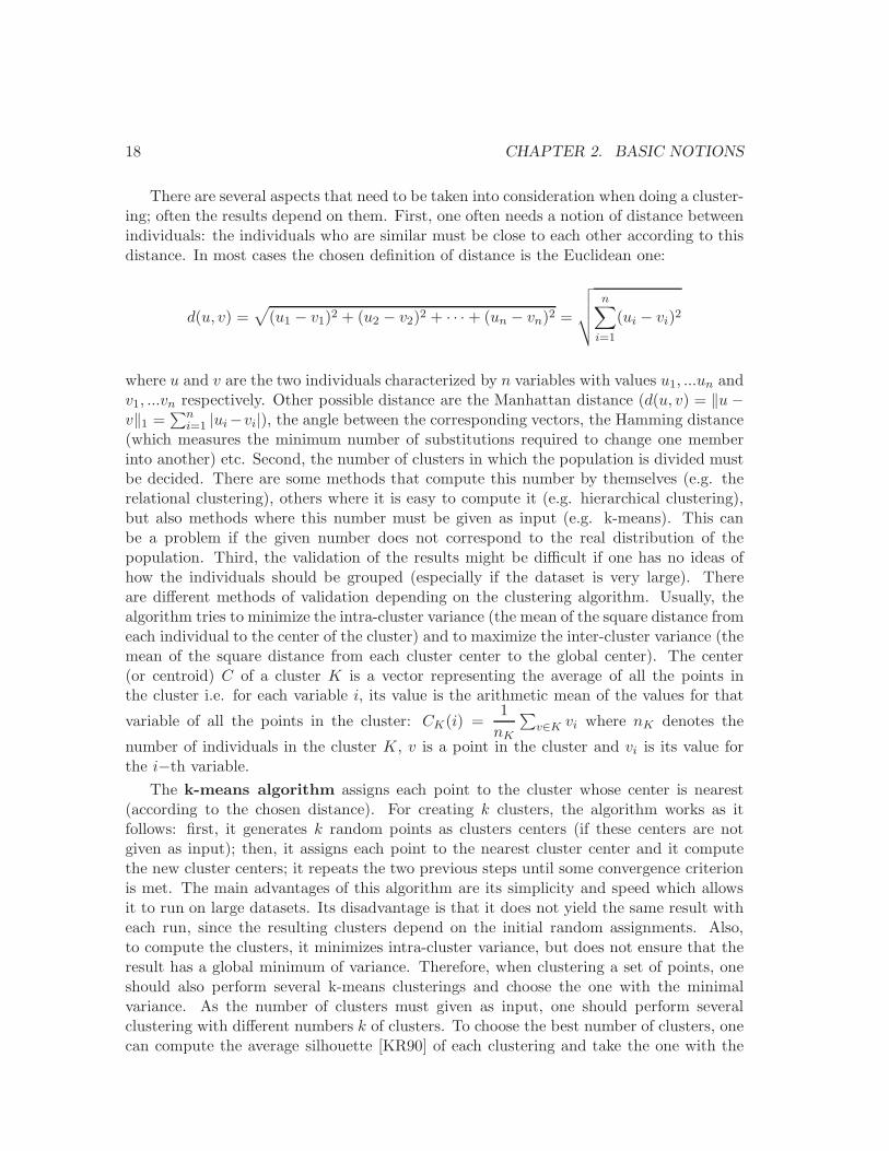
There are several aspects that need to be taken into consideration when doing a cluster-ing; often the results depend on them. First, one often needs a notion of distance betweenindividuals: the individuals who are similar must be close to each other according to thisdistance. In most cases the chosen definition of distance is the Euclidean one:
d(u, v) =√
(u1 − v1)2 + (u2 − v2)2 + · · ·+ (un − vn)2 =
√
√
√
√
n∑
i=1
(ui − vi)2
where u and v are the two individuals characterized by n variables with values u1, ...un andv1, ...vn respectively. Other possible distance are the Manhattan distance (d(u, v) = ‖u−v‖1 =
∑ni=1 |ui−vi|), the angle between the corresponding vectors, the Hamming distance
(which measures the minimum number of substitutions required to change one memberinto another) etc. Second, the number of clusters in which the population is divided mustbe decided. There are some methods that compute this number by themselves (e.g. therelational clustering), others where it is easy to compute it (e.g. hierarchical clustering),but also methods where this number must be given as input (e.g. k-means). This canbe a problem if the given number does not correspond to the real distribution of thepopulation. Third, the validation of the results might be difficult if one has no ideas ofhow the individuals should be grouped (especially if the dataset is very large). Thereare different methods of validation depending on the clustering algorithm. Usually, thealgorithm tries to minimize the intra-cluster variance (the mean of the square distance fromeach individual to the center of the cluster) and to maximize the inter-cluster variance (themean of the square distance from each cluster center to the global center). The center(or centroid) C of a cluster K is a vector representing the average of all the points inthe cluster i.e. for each variable i, its value is the arithmetic mean of the values for that
variable of all the points in the cluster: CK(i) =1
nK
∑
v∈K vi where nK denotes the
number of individuals in the cluster K, v is a point in the cluster and vi is its value forthe i−th variable.
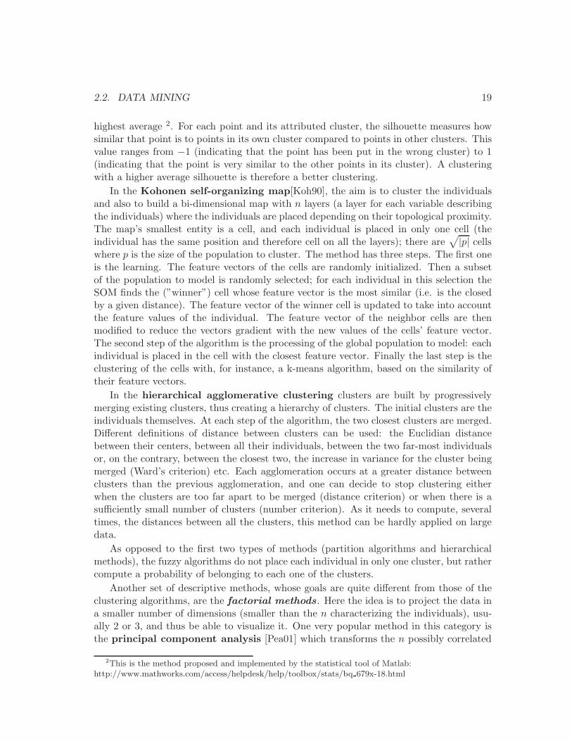
The k-means algorithm assigns each point to the cluster whose center is nearest(according to the chosen distance). For creating k clusters, the algorithm works as itfollows: first, it generates k random points as clusters centers (if these centers are notgiven as input); then, it assigns each point to the nearest cluster center and it computethe new cluster centers; it repeats the two previous steps until some convergence criterionis met. The main advantages of this algorithm are its simplicity and speed which allowsit to run on large datasets. Its disadvantage is that it does not yield the same result witheach run, since the resulting clusters depend on the initial random assignments. Also,to compute the clusters, it minimizes intra-cluster variance, but does not ensure that theresult has a global minimum of variance. Therefore, when clustering a set of points, oneshould also perform several k-means clusterings and choose the one with the minimalvariance. As the number of clusters must given as input, one should perform severalclustering with different numbers k of clusters. To choose the best number of clusters, onecan compute the average silhouette [KR90] of each clustering and take the one with the
2.2. DATA MINING 19
highest average 2. For each point and its attributed cluster, the silhouette measures howsimilar that point is to points in its own cluster compared to points in other clusters. Thisvalue ranges from −1 (indicating that the point has been put in the wrong cluster) to 1(indicating that the point is very similar to the other points in its cluster). A clusteringwith a higher average silhouette is therefore a better clustering.
In the Kohonen self-organizing map[Koh90], the aim is to cluster the individualsand also to build a bi-dimensional map with n layers (a layer for each variable describingthe individuals) where the individuals are placed depending on their topological proximity.The map’s smallest entity is a cell, and each individual is placed in only one cell (theindividual has the same position and therefore cell on all the layers); there are
√
|p| cellswhere p is the size of the population to cluster. The method has three steps. The first oneis the learning. The feature vectors of the cells are randomly initialized. Then a subsetof the population to model is randomly selected; for each individual in this selection theSOM finds the (”winner”) cell whose feature vector is the most similar (i.e. is the closedby a given distance). The feature vector of the winner cell is updated to take into accountthe feature values of the individual. The feature vector of the neighbor cells are thenmodified to reduce the vectors gradient with the new values of the cells’ feature vector.The second step of the algorithm is the processing of the global population to model: eachindividual is placed in the cell with the closest feature vector. Finally the last step is theclustering of the cells with, for instance, a k-means algorithm, based on the similarity oftheir feature vectors.
In the hierarchical agglomerative clustering clusters are built by progressivelymerging existing clusters, thus creating a hierarchy of clusters. The initial clusters are theindividuals themselves. At each step of the algorithm, the two closest clusters are merged.Different definitions of distance between clusters can be used: the Euclidian distancebetween their centers, between all their individuals, between the two far-most individualsor, on the contrary, between the closest two, the increase in variance for the cluster beingmerged (Ward’s criterion) etc. Each agglomeration occurs at a greater distance betweenclusters than the previous agglomeration, and one can decide to stop clustering eitherwhen the clusters are too far apart to be merged (distance criterion) or when there is asufficiently small number of clusters (number criterion). As it needs to compute, severaltimes, the distances between all the clusters, this method can be hardly applied on largedata.
As opposed to the first two types of methods (partition algorithms and hierarchicalmethods), the fuzzy algorithms do not place each individual in only one cluster, but rathercompute a probability of belonging to each one of the clusters.
Another set of descriptive methods, whose goals are quite different from those of theclustering algorithms, are the factorial methods. Here the idea is to project the data ina smaller number of dimensions (smaller than the n characterizing the individuals), usu-ally 2 or 3, and thus be able to visualize it. One very popular method in this category isthe principal component analysis [Pea01] which transforms the n possibly correlated
2This is the method proposed and implemented by the statistical tool of Matlab:http://www.mathworks.com/access/helpdesk/help/toolbox/stats/bq 679x-18.html
20 CHAPTER 2. BASIC NOTIONS
variables into a smaller number of uncorrelated variables called principal components. Thefirst principal component accounts for as much of the variability in the data as possible,and each succeeding component accounts for as much of the remaining variability as pos-sible. The new variables are linear combinations of the initial variables. By computing thevalues of these new variables for each individual, one has a representation of the individ-uals in a smaller number of variables. One can also plot them in a 2D-space representedby the first two principal components and thus have an image of the similarity betweenindividuals.
Predictive methods
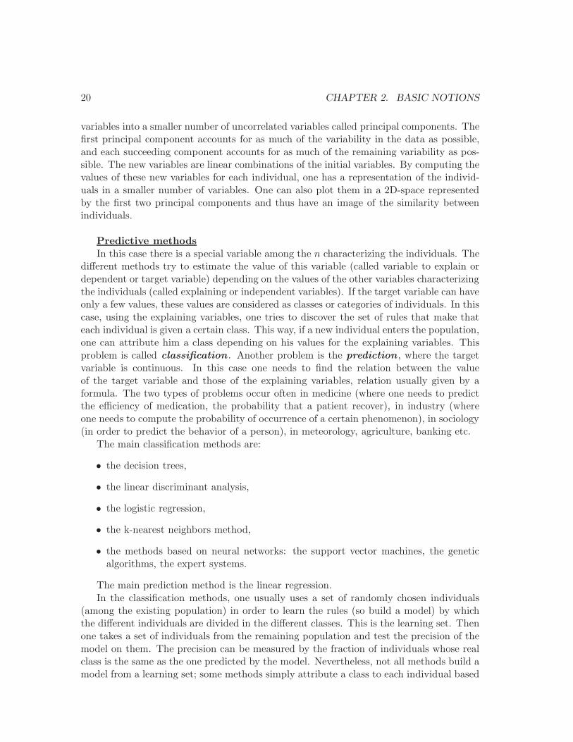
In this case there is a special variable among the n characterizing the individuals. Thedifferent methods try to estimate the value of this variable (called variable to explain ordependent or target variable) depending on the values of the other variables characterizingthe individuals (called explaining or independent variables). If the target variable can haveonly a few values, these values are considered as classes or categories of individuals. In thiscase, using the explaining variables, one tries to discover the set of rules that make thateach individual is given a certain class. This way, if a new individual enters the population,one can attribute him a class depending on his values for the explaining variables. Thisproblem is called classification . Another problem is the prediction , where the targetvariable is continuous. In this case one needs to find the relation between the valueof the target variable and those of the explaining variables, relation usually given by aformula. The two types of problems occur often in medicine (where one needs to predictthe efficiency of medication, the probability that a patient recover), in industry (whereone needs to compute the probability of occurrence of a certain phenomenon), in sociology(in order to predict the behavior of a person), in meteorology, agriculture, banking etc.
The main classification methods are:
• the decision trees,
• the linear discriminant analysis,
• the logistic regression,
• the k-nearest neighbors method,
• the methods based on neural networks: the support vector machines, the geneticalgorithms, the expert systems.
The main prediction method is the linear regression.In the classification methods, one usually uses a set of randomly chosen individuals
(among the existing population) in order to learn the rules (so build a model) by whichthe different individuals are divided in the different classes. This is the learning set. Thenone takes a set of individuals from the remaining population and test the precision of themodel on them. The precision can be measured by the fraction of individuals whose realclass is the same as the one predicted by the model. Nevertheless, not all methods build amodel from a learning set; some methods simply attribute a class to each individual based
2.2. DATA MINING 21
on some measures and not on a set of rules. For instance, the method of the k-nearestneighbors attributes to each individual the class of the k nearest individuals from him(according to a distance e.g. the Euclidian one). However, the choice of k, of the distanceto use and the fact that the classification of each new individual requires the manipulationof a whole set of already classified individuals make this method difficult to use. Oneusually prefers the methods where a model is built, especially when classifying large data.
A decision tree is used in order to find a set of rules that associate each individual to aclass. It begins by identifying the variable that divides best the individuals in the differentclasses such that one obtains some sub-populations, called nodes. The population of eachnode is then divided in other nodes based on the variable that splits best the individualsin classes. This is repeated until no division is possible or wanted. By construction, thefinal nodes (the leaves) contain mainly individuals of a single class. Each individual isassociated to a leaf, so to a certain class, with a rather high probability when he fulfillsthe set of rules allowing to get from the root to that leaf. The set of rules of all the leavesrepresents the classification model, used to attribute classes to new individuals. Thismethod is fast and the classification rules are easy to understand. Moreover it does notrequire any special conditions for the explaining variables (as for instance some probabilitylaws or absence of collinearity). However, each level of the tree depends on the previousone, which makes that the tree might find local optimums instead of global ones.
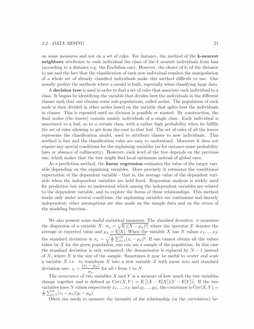
As a prediction method, the linear regression estimates the value of the target vari-able depending on the explaining variables. More precisely it estimates the conditionalexpectation of the dependent variable - that is, the average value of the dependent vari-able when the independent variables are held fixed. Regression analysis is widely usedfor prediction but also to understand which among the independent variables are relatedto the dependent variable, and to explore the forms of these relationships. This methodworks only under several conditions: the explaining variables are continuous and linearlyindependent; other assumptions are also made on the sample data and on the errors ofthe modeling function.
We also present some useful statistical measures. The standard deviation σ measuresthe dispersion of a variable X: σx =
√
E [(X − µx)2] where the operator E denotes theaverage or expected value and µx = E[X]. When the variable X has N values x1, ..., xN
the standard deviation is σx =√
1N
∑Ni=1(xi − µx)2. If one cannot obtain all the values
taken by X for the given population, one can use a sample of the population. In this casethe standard deviation is only estimated; the denominator is replaced by N − 1 insteadof N , where N is the size of the sample. Sometimes it may be useful to center and scalea variable X i.e. to transform X into a new variable Z with mean zero and standard
deviation one: zi =(xi − µx)
σxfor all i from 1 to N.
The covariance of two variables X and Y is a measure of how much the two variableschange together and is defined as Cov(X,Y ) = E
[
(X − E[X])(Y − E[Y ])]
. If the twovariables haveN values respectively x1, ..., xN and y1, ..., yN , the covariance is Cov(X,Y ) =1N
∑Ni=1(xi − µx)(yi − µy).
Often one needs to measure the intensity of the relationship (or the correlation) be-
22 CHAPTER 2. BASIC NOTIONS
tween two variables X and Y . If the two variables are continuous, this can be done bycomputing the linear correlation coefficient (also called Pearson correlation) rxy between
the two variables: rX,Y = corr(X,Y ) = cov(X,Y )σxσy
=E[(X−µx)(Y −µy)]
σxσy. The Pearson correla-
tion is +1 in the case of a perfect increasing (positive) linear relationship, −1 in the caseof a perfect decreasing (negative) linear relationship, and some value between −1 and 1in all the other cases, indicating the degree of linear dependence between the variables.As it approaches zero the correlation is weaker. The closer the coefficient is to either −1or 1, the stronger the correlation between the variables. If the two variables take only afew values (i.e. they represent classes or categories), one can verify if the two variablesare independent by performing a χ2 test (read chi-square). One can use this test to de-cide if the category X dependents on the class Y to which the individual belongs. If oneneeds to measure the correlation between a continuous variable and a categorization, onecan perform a ANOVA test. This test tells if the mean of the continuous variable is thesame for the different categories. If this is true then the two variables are independent.For instance, one can use the ANOVA test in order to see if the salary (the continuousvariable) is independent from the gender (the categories, male and female). However, thistest says only if the means are different or not, but it does not say for which categoriesthe means are significantly different and for which they are not. A test that can providesuch information is called a multiple comparison test . Such tests are the Bonferroni andthe Scheffe tests.
The χ2 and the ANOVA are exemples of hypothesis tests. Such tests are used toprove a given hypothesis H1. For that, one submits the opposite hypothesis H0 to a testT that must be satisfied if H0 is true. The idea is to show that T is not satisfied whichmeans that H0 is false, so H1 is true. H0 is called the null hypothesis while H1 is calledthe alternative hypothesis. To build the test T , one associates a statistic to H0 using theobservations; this statistic must follow a theoretical law if H0 is true. Next one measuresthe value v of the statistic on the given data and compares this value to the theoreticalvalues of the law. Also one chooses a significance level as a threshold from which thehypothesis is rejected; usually this value is at most 0.05. Now one computes the p-valuewhich is the probability to observe such a value as v if H0 is true. If this probability islower than the significance level, the null hypothesis H0 is rejected, so H1 is accepted. Onthe contrary, if the p−value is higher than the significance level, the null hypothesis can’tbe rejected, so one does not know if H1 is true.
Chapter 3
Complex networks
Informally, complex networks are modeling of large data. In many domains, sets of objectsand relations between them can be modeled as graphs where the vertices are the objectsand the edges correspond to relations. At the end of the 1990’s, due to the exponentialgrowth of the size of relational databases, along with the development of communicationtools, researchers began to analyze graphs modeling large datasets (with at least severalthousands of recordings). Although graph theory has a long tradition, the analysis ofgraphs modeling large datasets became a new field of study which began to develop veryfast, being surrounded by a lot of excitement. This is due not just to the development ofpowerful computers able to store and handle such large datasets but also (and especially)to the discovery of a set of properties shared by these graphs. Large graphs (and by largewe mean at least 105 vertices and edges) modeling datasets from numerous domains suchas biology, linguistics, inter-personal communication, WWW etc. are constantly found toshare several characteristics [BA99, WS98, New03]. They are therefore grouped under acommon name, that of complex networks.
There are numerous examples of complex networks extracted from real-life phenomena.They can model for instance the presence of words in sentences, interactions betweenproteins, collaborations between boards of directors, traces of phone calls or online activity,mobility dynamics of people, connections by plane between airports etc. They are theobject of study of many researchers, from several domains, going from computer scientists,mathematicians, physicists, to biologists, sociologists, economists etc. The interest comesfrom the importance of the study of such networks in understanding how nature works, howpeople interact, how different relations appear and evolve etc. Moreover these interactionsor relations are not random, they do not appear with an equal probability between twoobjects or two persons, but they are triggered by different factors. This was a majordiscovery in the analysis of complex networks: they are not random networks. Even more,as said before, they share several non-trivial properties. Almost every large network foundin nature, no matter its origin, follows a same set of characteristics. We detail theseproperties, along with computational issues and examples of complex networks presentingthem, in Section 3.1. We then present several models for network generation in Section 3.2.We finish this discussion on complex networks by showing some techniques for frequent
23
24 CHAPTER 3. COMPLEX NETWORKS
patterns discovery and motifs identification in Section 3.3.
3.1 Complex networks properties
We present several properties shared by most complex networks, there values in randomlygenerated networks, some computational aspects and real-world examples.
In this section on complex networks properties, by randomly generated graph we meana graph where no particular constraint is imposed (besides the number of vertices andedges): there can be an edge between each pair of vertices with the same probability. Thismodel of graph generation was introduced by Erdos and Renyi [ER60] and is a pioneerwork in the domain. The idea is very simple: we start with n nodes and we add edges suchthat, for each pair of nodes, an edge is added with equal probability p. This defines a setof graphs G(n, p) where (n, p) are the parameters of the model. Such graphs have someinteresting properties that we present in the same time as those of real-world networks.
For a graph G = (V,E), let n denote its number of vertices (i.e. n = |V |) and m itsnumber of edges (i.e. m = |E|).
Graphs randomly generated by the Erdos-Renyi model are used for comparisons withreal networks: for each real graph with n vertices and m edges, one generates random
graphs G(n, p) with p =2m
n(n− 1), so graphs that have the same number of vertices and
edges as the original one. Several characteristics are found to be shared by real-worldnetworks but not by the randomly generated graphs. We present here each one of thesecharacteristics, their values in several examples from real life and in random graphs butalso existing methods for their computation in large graphs. Remember that we computethese properties in graphs that have typically at least 105 vertices and an even highernumber of edges. A computation that takes O(n2) time (with n the number of vertices)is impractical for such graphs. Therefore one needs to use efficient (preferentially linear)algorithms when analyzing complex networks.
Degree distribution.
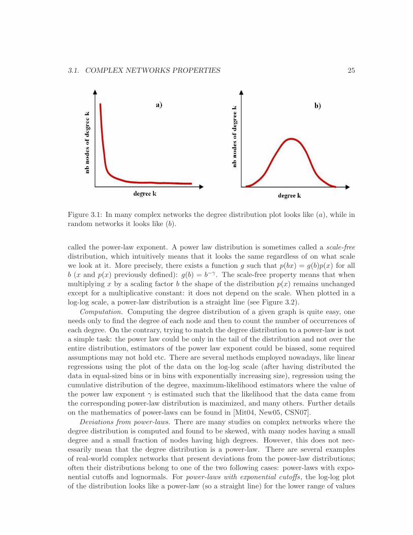
Definition. Generally in complex networks most nodes have very low degrees whilethere is a small fraction of nodes with very high degrees. When plotting the distributionof degrees, one obtains a curve that is very close to the axis (see Figure 3.1(a)). Thisis very different from the binomial degree distribution of random networks (see Figure3.1(b)); in these random graphs the probability that a node has degree k is
P (degree(v) = k) =
(
n− 1
k
)
pk(1− p)n−1−k.
On the contrary, many real-world graphs have degree distributions with probability densityfunctions of the form
p(x) = ax−γ
where p(x) is the probability to encounter the value x, a is a constant and γ is an expo-nent; distributions with such probability density functions are called power-laws and γ is
3.1. COMPLEX NETWORKS PROPERTIES 25
Figure 3.1: In many complex networks the degree distribution plot looks like (a), while inrandom networks it looks like (b).
called the power-law exponent. A power law distribution is sometimes called a scale-freedistribution, which intuitively means that it looks the same regardless of on what scalewe look at it. More precisely, there exists a function g such that p(bx) = g(b)p(x) for allb (x and p(x) previously defined): g(b) = b−γ . The scale-free property means that whenmultiplying x by a scaling factor b the shape of the distribution p(x) remains unchangedexcept for a multiplicative constant: it does not depend on the scale. When plotted in alog-log scale, a power-law distribution is a straight line (see Figure 3.2).
Computation. Computing the degree distribution of a given graph is quite easy, oneneeds only to find the degree of each node and then to count the number of occurrences ofeach degree. On the contrary, trying to match the degree distribution to a power-law is nota simple task: the power law could be only in the tail of the distribution and not over theentire distribution, estimators of the power law exponent could be biased, some requiredassumptions may not hold etc. There are several methods employed nowadays, like linearregressions using the plot of the data on the log-log scale (after having distributed thedata in equal-sized bins or in bins with exponentially increasing size), regression using thecumulative distribution of the degree, maximum-likelihood estimators where the value ofthe power law exponent γ is estimated such that the likelihood that the data came fromthe corresponding power-law distribution is maximized, and many others. Further detailson the mathematics of power-laws can be found in [Mit04, New05, CSN07].
Deviations from power-laws. There are many studies on complex networks where thedegree distribution is computed and found to be skewed, with many nodes having a smalldegree and a small fraction of nodes having high degrees. However, this does not nec-essarily mean that the degree distribution is a power-law. There are several examplesof real-world complex networks that present deviations from the power-law distributions;often their distributions belong to one of the two following cases: power-laws with expo-nential cutoffs and lognormals. For power-laws with exponential cutoffs, the log-log plotof the distribution looks like a power-law (so a straight line) for the lower range of values
26 CHAPTER 3. COMPLEX NETWORKS
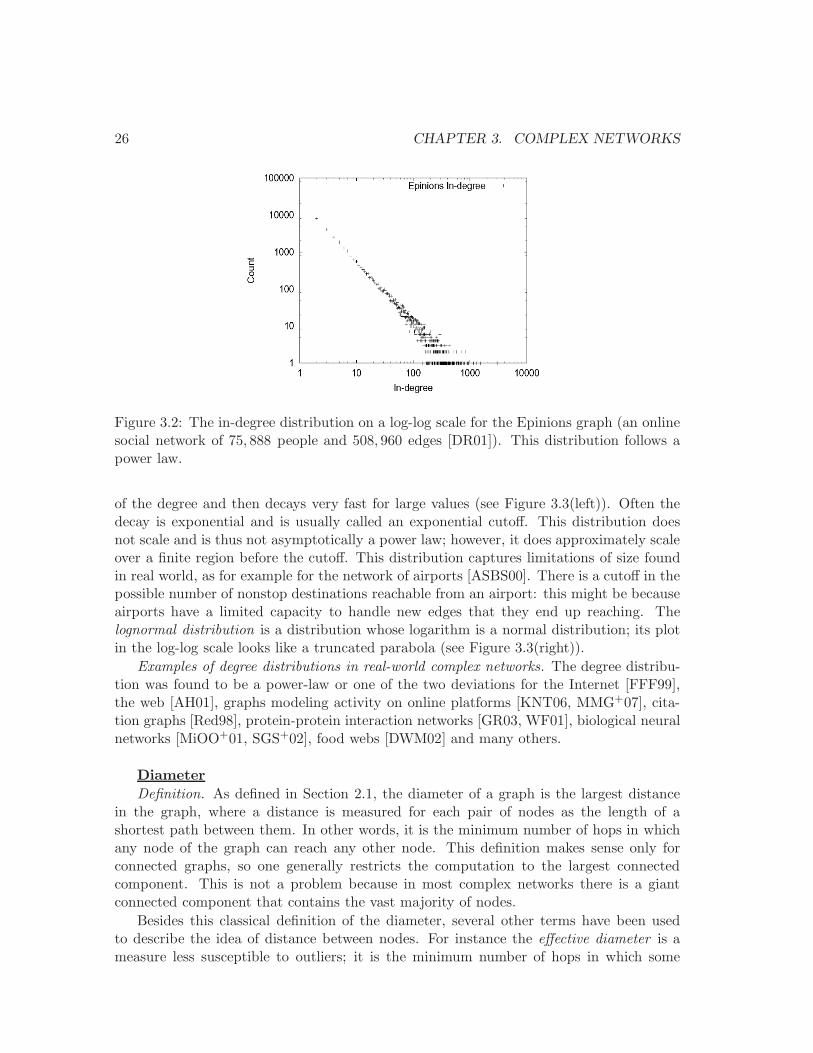
Figure 3.2: The in-degree distribution on a log-log scale for the Epinions graph (an onlinesocial network of 75, 888 people and 508, 960 edges [DR01]). This distribution follows apower law.
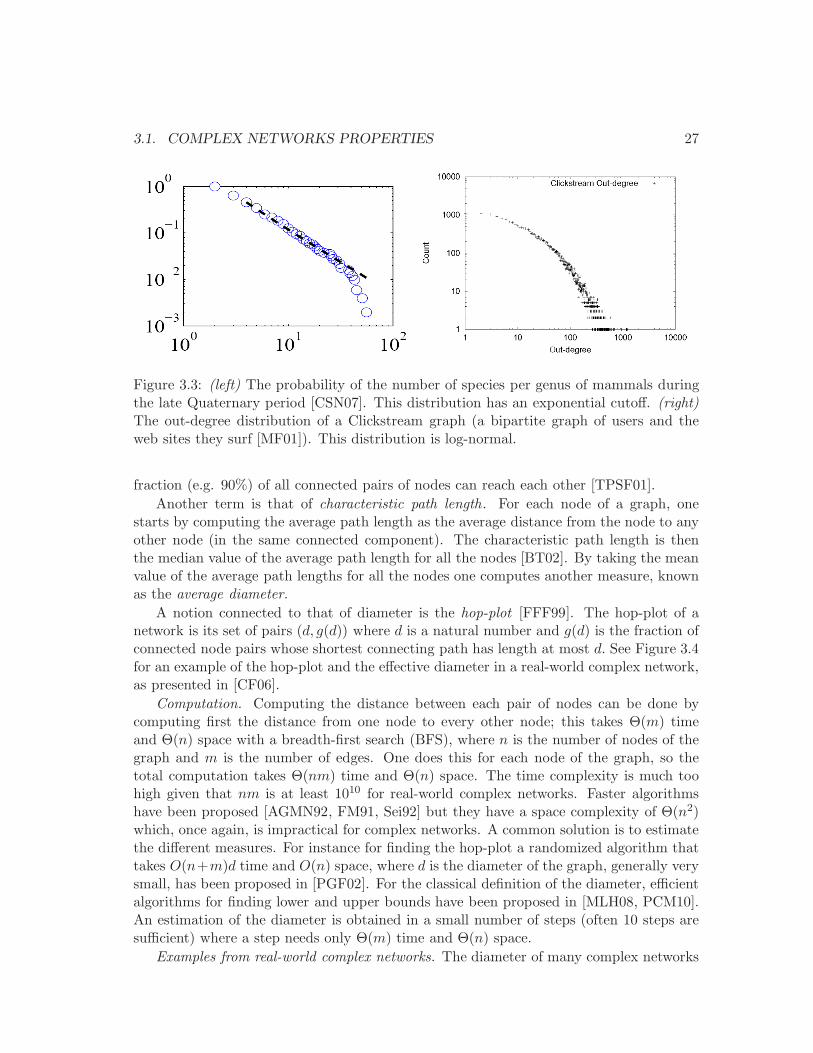
of the degree and then decays very fast for large values (see Figure 3.3(left)). Often thedecay is exponential and is usually called an exponential cutoff. This distribution doesnot scale and is thus not asymptotically a power law; however, it does approximately scaleover a finite region before the cutoff. This distribution captures limitations of size foundin real world, as for example for the network of airports [ASBS00]. There is a cutoff in thepossible number of nonstop destinations reachable from an airport: this might be becauseairports have a limited capacity to handle new edges that they end up reaching. Thelognormal distribution is a distribution whose logarithm is a normal distribution; its plotin the log-log scale looks like a truncated parabola (see Figure 3.3(right)).
Examples of degree distributions in real-world complex networks. The degree distribu-tion was found to be a power-law or one of the two deviations for the Internet [FFF99],the web [AH01], graphs modeling activity on online platforms [KNT06, MMG+07], cita-tion graphs [Red98], protein-protein interaction networks [GR03, WF01], biological neuralnetworks [MiOO+01, SGS+02], food webs [DWM02] and many others.
Diameter
Definition. As defined in Section 2.1, the diameter of a graph is the largest distancein the graph, where a distance is measured for each pair of nodes as the length of ashortest path between them. In other words, it is the minimum number of hops in whichany node of the graph can reach any other node. This definition makes sense only forconnected graphs, so one generally restricts the computation to the largest connectedcomponent. This is not a problem because in most complex networks there is a giantconnected component that contains the vast majority of nodes.
Besides this classical definition of the diameter, several other terms have been usedto describe the idea of distance between nodes. For instance the effective diameter is ameasure less susceptible to outliers; it is the minimum number of hops in which some
3.1. COMPLEX NETWORKS PROPERTIES 27
Figure 3.3: (left) The probability of the number of species per genus of mammals duringthe late Quaternary period [CSN07]. This distribution has an exponential cutoff. (right)The out-degree distribution of a Clickstream graph (a bipartite graph of users and theweb sites they surf [MF01]). This distribution is log-normal.
fraction (e.g. 90%) of all connected pairs of nodes can reach each other [TPSF01].
Another term is that of characteristic path length. For each node of a graph, onestarts by computing the average path length as the average distance from the node to anyother node (in the same connected component). The characteristic path length is thenthe median value of the average path length for all the nodes [BT02]. By taking the meanvalue of the average path lengths for all the nodes one computes another measure, knownas the average diameter.
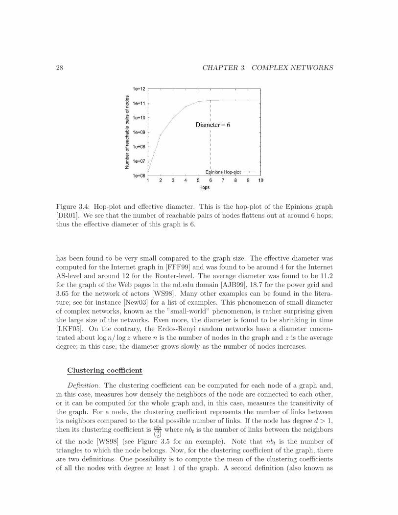
A notion connected to that of diameter is the hop-plot [FFF99]. The hop-plot of anetwork is its set of pairs (d, g(d)) where d is a natural number and g(d) is the fraction ofconnected node pairs whose shortest connecting path has length at most d. See Figure 3.4for an example of the hop-plot and the effective diameter in a real-world complex network,as presented in [CF06].
Computation. Computing the distance between each pair of nodes can be done bycomputing first the distance from one node to every other node; this takes Θ(m) timeand Θ(n) space with a breadth-first search (BFS), where n is the number of nodes of thegraph and m is the number of edges. One does this for each node of the graph, so thetotal computation takes Θ(nm) time and Θ(n) space. The time complexity is much toohigh given that nm is at least 1010 for real-world complex networks. Faster algorithmshave been proposed [AGMN92, FM91, Sei92] but they have a space complexity of Θ(n2)which, once again, is impractical for complex networks. A common solution is to estimatethe different measures. For instance for finding the hop-plot a randomized algorithm thattakes O(n+m)d time and O(n) space, where d is the diameter of the graph, generally verysmall, has been proposed in [PGF02]. For the classical definition of the diameter, efficientalgorithms for finding lower and upper bounds have been proposed in [MLH08, PCM10].An estimation of the diameter is obtained in a small number of steps (often 10 steps aresufficient) where a step needs only Θ(m) time and Θ(n) space.
Examples from real-world complex networks. The diameter of many complex networks
28 CHAPTER 3. COMPLEX NETWORKS
Figure 3.4: Hop-plot and effective diameter. This is the hop-plot of the Epinions graph[DR01]. We see that the number of reachable pairs of nodes flattens out at around 6 hops;thus the effective diameter of this graph is 6.
has been found to be very small compared to the graph size. The effective diameter wascomputed for the Internet graph in [FFF99] and was found to be around 4 for the InternetAS-level and around 12 for the Router-level. The average diameter was found to be 11.2for the graph of the Web pages in the nd.edu domain [AJB99], 18.7 for the power grid and3.65 for the network of actors [WS98]. Many other examples can be found in the litera-ture; see for instance [New03] for a list of examples. This phenomenon of small diameterof complex networks, known as the ”small-world” phenomenon, is rather surprising giventhe large size of the networks. Even more, the diameter is found to be shrinking in time[LKF05]. On the contrary, the Erdos-Renyi random networks have a diameter concen-trated about log n/ log z where n is the number of nodes in the graph and z is the averagedegree; in this case, the diameter grows slowly as the number of nodes increases.
Clustering coefficient
Definition. The clustering coefficient can be computed for each node of a graph and,in this case, measures how densely the neighbors of the node are connected to each other,or it can be computed for the whole graph and, in this case, measures the transitivity ofthe graph. For a node, the clustering coefficient represents the number of links betweenits neighbors compared to the total possible number of links. If the node has degree d > 1,then its clustering coefficient is nbt
(d2)where nbt is the number of links between the neighbors
of the node [WS98] (see Figure 3.5 for an exemple). Note that nbt is the number oftriangles to which the node belongs. Now, for the clustering coefficient of the graph, thereare two definitions. One possibility is to compute the mean of the clustering coefficientsof all the nodes with degree at least 1 of the graph. A second definition (also known as
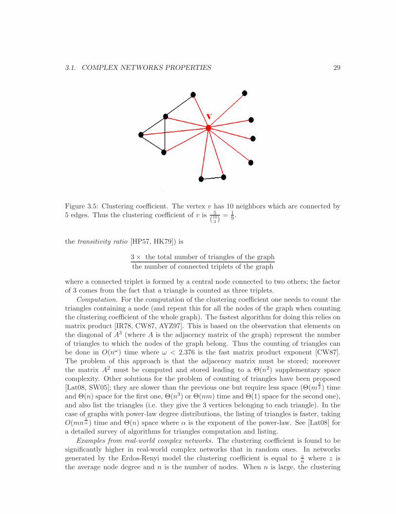
3.1. COMPLEX NETWORKS PROPERTIES 29
Figure 3.5: Clustering coefficient. The vertex v has 10 neighbors which are connected by5 edges. Thus the clustering coefficient of v is 5
(102)= 1
9 .
the transitivity ratio [HP57, HK79]) is
3× the total number of triangles of the graph
the number of connected triplets of the graph
where a connected triplet is formed by a central node connected to two others; the factorof 3 comes from the fact that a triangle is counted as three triplets.
Computation. For the computation of the clustering coefficient one needs to count thetriangles containing a node (and repeat this for all the nodes of the graph when countingthe clustering coefficient of the whole graph). The fastest algorithm for doing this relies onmatrix product [IR78, CW87, AYZ97]. This is based on the observation that elements onthe diagonal of A3 (where A is the adjacency matrix of the graph) represent the numberof triangles to which the nodes of the graph belong. Thus the counting of triangles canbe done in O(nω) time where ω < 2.376 is the fast matrix product exponent [CW87].The problem of this approach is that the adjacency matrix must be stored; moreoverthe matrix A2 must be computed and stored leading to a Θ(n2) supplementary spacecomplexity. Other solutions for the problem of counting of triangles have been proposed[Lat08, SW05]; they are slower than the previous one but require less space (Θ(m
3
2 ) timeand Θ(n) space for the first one, Θ(n3) or Θ(nm) time and Θ(1) space for the second one),and also list the triangles (i.e. they give the 3 vertices belonging to each triangle). In thecase of graphs with power-law degree distributions, the listing of triangles is faster, takingO(mn
1
α ) time and Θ(n) space where α is the exponent of the power-law. See [Lat08] fora detailed survey of algorithms for triangles computation and listing.
Examples from real-world complex networks. The clustering coefficient is found to besignificantly higher in real-world complex networks that in random ones. In networksgenerated by the Erdos-Renyi model the clustering coefficient is equal to z
nwhere z is
the average node degree and n is the number of nodes. When n is large, the clustering
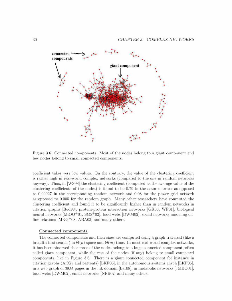
30 CHAPTER 3. COMPLEX NETWORKS
Figure 3.6: Connected components. Most of the nodes belong to a giant component andfew nodes belong to small connected components.
coefficient takes very low values. On the contrary, the value of the clustering coefficientis rather high in real-world complex networks (compared to the one in random networksanyway). Thus, in [WS98] the clustering coefficient (computed as the average value of theclustering coefficients of the nodes) is found to be 0.79 in the actor network as opposedto 0.00027 in the corresponding random network and 0.08 for the power grid networkas opposed to 0.005 for the random graph. Many other researchers have computed theclustering coefficient and found it to be significantly higher than in random networks incitation graphs [Red98], protein-protein interaction networks [GR03, WF01], biologicalneural networks [MiOO+01, SGS+02], food webs [DWM02], social networks modeling on-line relations [MKG+08, ABA03] and many others.
Connected components
The connected components and their sizes are computed using a graph traversal (like abreadth-first search ) in Θ(n) space and Θ(m) time. In most real-world complex networks,it has been observed that most of the nodes belong to a huge connected component, oftencalled giant component, while the rest of the nodes (if any) belong to small connectedcomponents, like in Figure 3.6. There is a giant connected component for instance incitation graphs (ArXiv and pattents) [LKF05], in the autonomous systems graph [LKF05],in a web graph of 39M pages in the .uk domain [Lat08], in metabolic networks [JMBO01],food webs [DWM02], email networks [NFB02] and many others.
3.1. COMPLEX NETWORKS PROPERTIES 31
In random graphs, for a low value of p, there are few edges and all the connectedcomponents are small, having an exponential size distribution with finite mean size. Forhigh values of p, the graphs have a giant component with O(n) of the nodes in the graphbelonging to this component (where n is the total number of nodes). The rest of the com-ponents again have an exponential size distribution with finite mean size. The changeover(called the phase transition) between these two regimes occurs at p = 1/N.
Communities
Communities (or modules or clusters) are groups of nodes better connected betweenthemselves (i.e. have more links) than to the rest of the network. A large body of work hasbeen devoted to defining and identifying communities in complex networks. There existsagglomerative methods (where nodes are grouped into hierarchies, which are groupedthemselves into high-level hierarchies and so on [Eve80]), divisive methods (where, startingwith the whole graph, edges are removed in a prescribed order based on a given measure, asfor instance edge-betweenness [GN02]), methods based on max-flow min-cut formulations[FLG00] or on Kirchoff’s laws [WH04], local methods (based on local information [Vir03]),optimization methods (based on the maximization of an objective function [CMN04]) andmany others. A very efficient algorithm for extracting communities in large graphs wasproposed in [BGLL08]. For a survey on community identification, see for instance [For10].
The quality of the partitions resulting from these methods is often measured by themodularity Q of the partition, a measure of the density of links inside communities ascompared to links between communities [New04, NG04]:
Q =1
2m
∑
ij
[
Aij −kikj2m
]
δ(ci, cj)
where m is the number of edges of the graph, Aij is the adjacency matrix, ki is the degreeof the node i, ci is the community to which the node i belongs and δ(ci, cj) is the Kroneckerdelta symbol, equal to 1 if ci = cj and to 0 otherwise.
As to the significance of the identified communities, it has been observed that community-like sets of nodes tend to correspond to organizational units in social networks [New06],functional modules in biological networks [RSM+02] and scientific disciplines in collabo-ration networks between scientists [GN02] (see Figure 3.7).
Centrality
The centrality is a measure of the relative importance of a node within a network.There are several definitions of centrality; here we present the most commonly used:
• the degree centrality,
• the betweenness,
• the closeness,
• the eigen vector centrality,
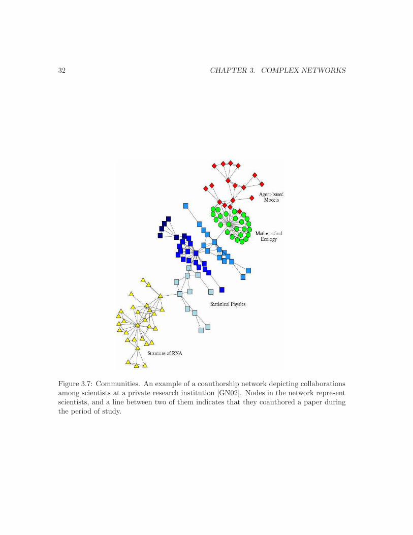
32 CHAPTER 3. COMPLEX NETWORKS
Figure 3.7: Communities. An example of a coauthorship network depicting collaborationsamong scientists at a private research institution [GN02]. Nodes in the network representscientists, and a line between two of them indicates that they coauthored a paper duringthe period of study.
3.1. COMPLEX NETWORKS PROPERTIES 33
• the page rank.
The degree centrality is the simplest one. It is defined as the number of links a nodehas (the degree of the node) divided by n− 1 where n is the number of nodes of the graph(this is just for normalization; this way the range of values of the degree centrality is 0to 1). Degree is often interpreted in terms of the immediate risk of a node for catchingwhatever is flowing through the network (such as a virus, or some information). Whilevery simple and easy to compute, this measure does not really capture the importance ofthe node as some very high-degree nodes might be placed at the periphery of the networkand thus be important only for a small part of the network. As explained in [Bar02], ifone measures the degree centrality of nodes in the movie actors network (where two actorsare connected by a link if they have acted together in a movie), the most central actorsare found to be porno actors. Their importance in the movie network is however limitedto the porno section and one can reasonably argue that there are other more importantactors.
The betweenness centrality [Fre77] considers as central nodes that are placed on manyshortest paths between other nodes; these nodes are important as one has to pass troughthem in order to travel efficiently in the different parts of the network. Thus, the between-ness centrality CB of a vertex v is defined as
CB(v) =∑
s6=v 6=t∈V
s6=t
σst(v)
σst
where σst is the number of shortest paths between s and t and σst(v) is the number of suchshortest paths that pass trough v. This measure reflects better the notion of importanceof a node than the previous one, but it is costly to compute (it takes O(nm) time usingthe most efficient known algorithm [Bra01]) and thus difficult to use on large networks.
The closeness centrality considers as central nodes that are at a short distance from theother nodes (in the same connected component); thus the closeness of a node is the sumof the distances between this node and all the other nodes in its connected componentdivided by the number of nodes in the component (minus 1, as one does not take intoconsideration the node itself). Closeness can be regarded as a measure of how long it willtake information to spread from a given node to other reachable nodes in the network.Computing the closeness means computing the shortest distance from one node to the otherones which can be done for each node in Θ(m) time and Θ(n) space with a breadth-firstsearch (BFS). As the closeness of a node makes sense when compared to that of other nodesof the graph, one needs to compute it for (all the) other nodes of the graph, so the timecomplexity is multiplied by the number of nodes. An efficient randomized approximationalgorithm for computing closeness centrality in weighted graphs has been proposed in[EW04]; this algorithm estimates the centrality of all vertices with high probability withina (1 + ǫ) factor, ǫ > 0, in near-linear time. See Figure 3.8 for an example of graph andTable 3.1 for the values of the degree, the betweenness and the closeness centrailty in thisgraph.
The eigen vector centrality [Bon87] and the page rank [BP98] assign relative scores toall nodes in the network based on the principle that connections to high-scoring nodes
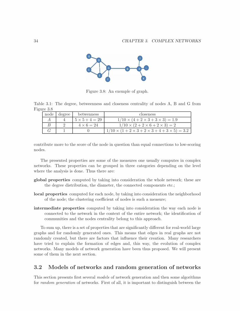
34 CHAPTER 3. COMPLEX NETWORKS
Figure 3.8: An exemple of graph.
Table 3.1: The degree, betweenness and closeness centrality of nodes A, B and G fromFigure 3.8
node degree betwenness closeness
A 4 5× 5 + 4 = 29 1/10 × (4 + 2× 3 + 3× 3) = 1.9
B 2 4× 6 = 24 1/10 × (2 + 2× 6 + 2× 3) = 2
G 1 0 1/10 × (1 + 2× 3 + 2× 3 + 4 + 3× 5) = 3.2
contribute more to the score of the node in question than equal connections to low-scoringnodes.
The presented properties are some of the measures one usually computes in complexnetworks. These properties can be grouped in three categories depending on the levelwhere the analysis is done. Thus there are:
global properties computed by taking into consideration the whole network; these arethe degree distribution, the diameter, the connected components etc.;
local properties computed for each node, by taking into consideration the neighborhoodof the node; the clustering coefficient of nodes is such a measure;
intermediate properties computed by taking into consideration the way each node isconnected to the network in the context of the entire network; the identification ofcommunities and the nodes centrality belong to this approach.
To sum up, there is a set of properties that are significantly different for real-world largegraphs and for randomly generated ones. This means that edges in real graphs are notrandomly created, but there are factors that influence their creation. Many researchershave tried to explain the formation of edges and, this way, the evolution of complexnetworks. Many models of network generation have been thus proposed. We will presentsome of them in the next section.
3.2 Models of networks and random generation of networks
This section presents first several models of network generation and then some algorithmsfor random generation of networks. First of all, it is important to distinguish between the
3.2. MODELS OF NETWORKS AND RANDOM GENERATION OF NETWORKS 35
two approaches. In the construction of models of networks, the goal is, given an originalnetwork, to explain the formation of its links. Therefore one can generate an artificialnetwork from one vertex to a complex object where the resulting network reproduces sev-eral properties of the original one. However, the resulting network is not randomly chosenamong all the networks with those properties. That is, there may be some networks thatshare all the input properties but who never get generated by the model. This is not aproblem since the model does not try to generate all the possible networks with the inputproperties but to give an explanation for the formation of links in the original network.On the contrary, the goal of the random generation of networks is precisely to generatenetworks that are randomly (i.e. with the same probability) chosen among all the networksthat have the input properties. In this case, any network with those properties is gener-ated with an equal probability. If the first approach proposes models in order to explainthe formation of links and therefore the evolution of the network, the second approachproposes generations of networks that are then used as null models. That is, they are usedas a general characterization of all the networks with the input set of properties. One canuse the null model in order to see if the original network has some other properties thatdistinguish it from the null model (or, on the contrary, it is just one ordinary networkwith the input properties).
Models of networks
The simplest model of network is the Erdos-Renyi model that was discussed earlier.In this model no condition is imposed for the formation of links: any two nodes can beconnected by a link with the same probability. However, the graphs generated by thismodel are very different from real-world complex networks. Therefore there must be alogic, a reason behind the formation of links: the links are not randomly created butgenerated by one or several factors.
The first model of graph generation after the Erdos-Renyi model was that proposedby Watts and Strogatz [WS98]. This model, introduced nearly 40 years after that ofErdos and Renyi, was the first one to generate graphs sharing some of the properties ofreal-world complex networks. In this model links do not connect random pairs of nodes,but each node is connected to k of its closest neighbors (nodes are displayed on a circle).Next, for each node u, each of its edges (u, v) is rewired with probability p to form somedifferent edge (u,w), where node w is chosen uniformly at random. The parameter p givesthe randomness of the generated graph: when p = 0 the graph is completely ordered andwhen p = 1 the graph is completely random. Between the two, there is a broad region ofvalues of p in which the clustering coefficient of the network is rather high and the averageshortest path length is low.
Another model introduced just after that of Watts and Strogatz tried to explain an-other property of large complex-networks: the heterogeneous right skewed distribution ofthe degree. This model, introduced in [BA99] and known as the ”preferential attachmentmodel”, contains two mechanisms: population growth and preferential attachment. Theintuition behind the first mechanism is straightforward: real networks grow in time as newmembers join the population. The mechanism of preferential attachment, analogous to Si-mon’s ”Gibrat principle” [Sim55b] and Merton’s ”Matthew Effect” [Mer68], expresses the
36 CHAPTER 3. COMPLEX NETWORKS
idea that newly arriving nodes will tend to connect to already well-connected nodes ratherthan poorly connected ones. Specifically, Barabasi and Albert defined the probability thata new node connects to an existing node with degree d as c× d (where c is a normalizingconstant). Barabasi and Albert showed that over a sufficiently long time horizon, thedegree distribution of a growing network exhibiting linear preferential attachment wouldconverge to a power-law with exponent γ = 3.
The graphs generated by the two models, however, do not exhibit all the propertiesof real-world complex networks. In the first model, the shape of the degree distributionis similar to that of random graphs generated by the Erdos-Renyi model. For the graphsgenerated by the second model, the power-law exponent of the degree distribution is fixedat γ = 3 (while many real-world graphs deviate from this value), there is exactly oneconnected component (while many real-world graphs have several isolated components),the average degree is constant (while the average degree of some real-world graphs increasesover time [BJN+02, LKF05]).
Many other models have been proposed since these two initial ones. Each model triesto explain different properties observed in real-world complex networks as for instancethe shrinking diameter (this is done by the forest fire model proposed in [LKF05]), theincreasing average degree (this is done by the model proposed in [BJN+02]), communitybehavior (two models [KKR+99, KRRT99] try to explain this) and many others. See forinstance [CF06] for a detailed presentation of existing network models.
Random generation of networks
Given a set of properties, a generator of random graphs must produce graphs thatare randomly chosen among all the graphs presenting that set of properties. Usually theproperties are computed in an input graph for which one needs to build null models.Several existing generators produce graphs that preserve the degree distribution of theinput graph. It is the case for instance of the generator introduced in [VL05] 1 thatgenerates simple connected graphs; this generator needs as input a set of pairs of degreeand number of vertices with that degree. Another generator that preserves, for each node,its in-degree and its out-degree, was used in [MSOI+02] 2; graphs generated this wayserved as null model for finding network motifs as we explain in the following section.
Sometimes one needs to generate graphs that have not just a given degree distributionbut also other properties. We present here a generator introduced in [MKFV06] 3 basedon dk − series.
The algorithm introduced in [MKFV06] generates graphs that preserve the dk-series dis-tribution of the given input graph. dK−series describe correlations amongst degrees of nodesin subgraphs of size d, for d = 0, 1, ..., n. For instance, when d = 3 and the input graph is undi-rected, the 3k−distribution contains the number of connected triplets with degrees k1, k2, k3for all k1, k2, k3 ∈ N. The connected triplets can be triangles and 3−nodes paths, so onecounts separately the triangles and the 3−nodes paths with degrees k1, k2, k3. The generated
1Tool available at http://fabien.viger.free.fr/liafa/generation/2Tool available at http://www.weizmann.ac.il/mcb/UriAlon/3Tool available at http://www.sysnet.ucsd.edu/ pmahadevan/topo research/topo.html
3.3. IDENTIFICATION OF PATTERNS IN COMPLEX NETWORKS 37
graphs that preserve the 3k-serie of the input graph will have the same number of trianglesand of 3−nodes paths as the input graph; moreover the connected 3−nodes subgraphs of thegenerated graphs will have exactly the same combinations of degrees as the input graph.
When d = 0, the generated graphs have the same average degree as the input one. Whend = 1 the degree distribution is preserved. When d = 2, the generated graphs have the samenumber of edges with degrees k1, k2 for all k1, k2 ∈ N. The dk-series have two importantproperties: first, graphs having a dk-distribution also have the d’k-distributions, with d′ < d;second, generated graphs are more and more similar to the input graph when d increases,ending up isomorphic to it when d = n. Using this approach, the authors construct graphsfor d = 0, 1, 2, 3 and demonstrate that these graphs reproduce, with increasing accuracy,important properties of measured and modeled Internet topologies. They find that the d = 2case is sufficient for most practical purposes, while d = 3 essentially reconstructs the InternetAS- and router-level topologies.
3.3 Identification of patterns in complex networks
Frequent patternsIn numerous analysis like mining biochemical structures, program flow control study,
graph comparison or compression etc., one needs to compute the number of occurrences ofa graph Q as subgraph in the graphs G1, G2, ...Gn of a given database D. This is the graphquery problem. Often one needs to solve a problem close to this one, the frequent graphpatterns problem, where one computes all the graphs Q that are subgraph of a numberof graphs in D, this number being higher than a given threshold (this number is calledthe support of Q). There are several algorithms for solving these problems; they can begrouped in:
• graph-theory based algorithms,
• greedy algorithms,
• algorithms using inductive logic programming.
For the graph-theory based algorithms, one usually follows the general principal of theApriori algorithm introduced in [AS94] for association rule mining: in a ”bottom up”approach, frequent subsets (here graphs) are extended one item at a time (a step knownas candidate generation), then candidates are tested against the data. The algorithmterminates when no further successful extensions are found. For instance, AGM [IWM00]is an algorithm based on this idea that uses canonical codes for adjacency matrices andtherefore for subgraph matching. Frequent subgraphs are generated in the bottom-uporder by adding one vertex at a time (two already found frequent graphs with the samenumber of vertices are joined together in a candidate graph that has one more vertex).However this algorithm suffers from computational intractability when the graph becomestoo large. Another algorithm, FSG proposed in [KK01], uses the same scheme: startingwith frequent graphs with 1 and 2 nodes, it successively generates larger frequent graphsby adding one edge at a time. The algorithm expects a graph with colored edges and
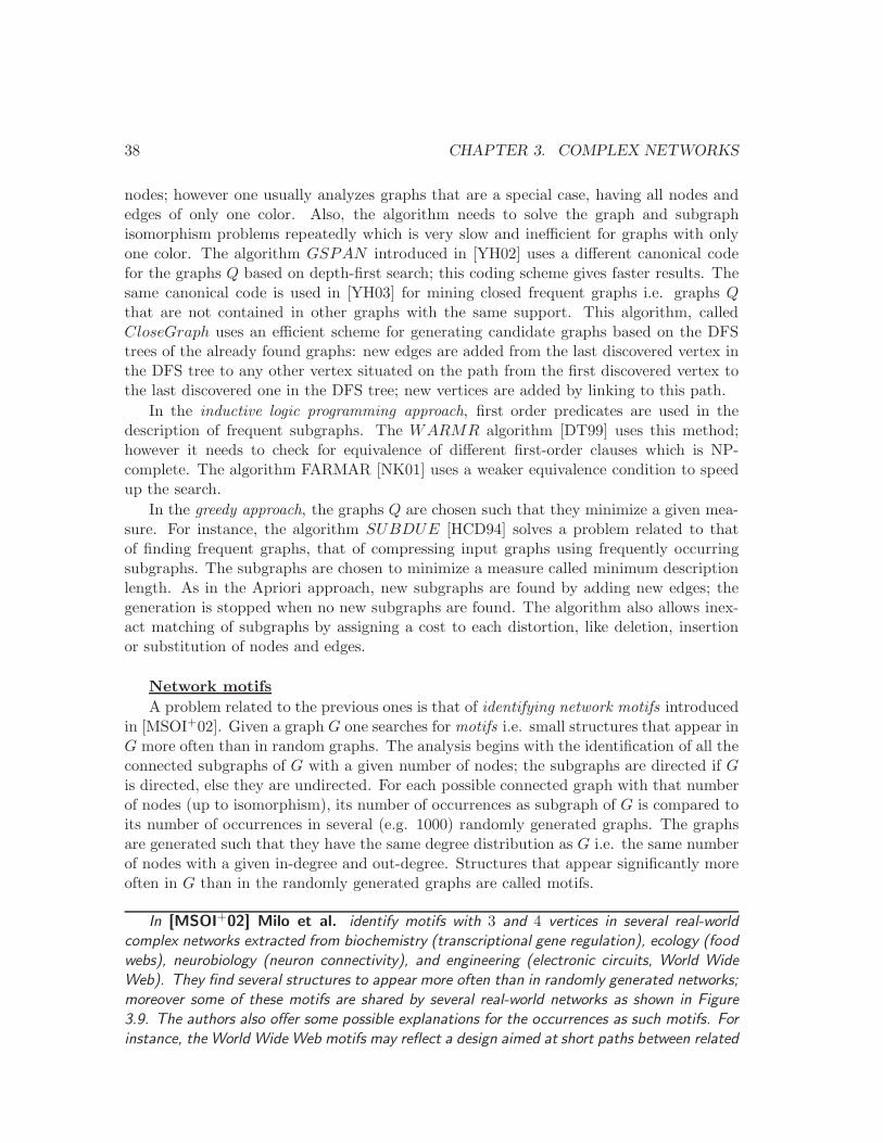
38 CHAPTER 3. COMPLEX NETWORKS
nodes; however one usually analyzes graphs that are a special case, having all nodes andedges of only one color. Also, the algorithm needs to solve the graph and subgraphisomorphism problems repeatedly which is very slow and inefficient for graphs with onlyone color. The algorithm GSPAN introduced in [YH02] uses a different canonical codefor the graphs Q based on depth-first search; this coding scheme gives faster results. Thesame canonical code is used in [YH03] for mining closed frequent graphs i.e. graphs Qthat are not contained in other graphs with the same support. This algorithm, calledCloseGraph uses an efficient scheme for generating candidate graphs based on the DFStrees of the already found graphs: new edges are added from the last discovered vertex inthe DFS tree to any other vertex situated on the path from the first discovered vertex tothe last discovered one in the DFS tree; new vertices are added by linking to this path.
In the inductive logic programming approach, first order predicates are used in thedescription of frequent subgraphs. The WARMR algorithm [DT99] uses this method;however it needs to check for equivalence of different first-order clauses which is NP-complete. The algorithm FARMAR [NK01] uses a weaker equivalence condition to speedup the search.
In the greedy approach, the graphs Q are chosen such that they minimize a given mea-sure. For instance, the algorithm SUBDUE [HCD94] solves a problem related to thatof finding frequent graphs, that of compressing input graphs using frequently occurringsubgraphs. The subgraphs are chosen to minimize a measure called minimum descriptionlength. As in the Apriori approach, new subgraphs are found by adding new edges; thegeneration is stopped when no new subgraphs are found. The algorithm also allows inex-act matching of subgraphs by assigning a cost to each distortion, like deletion, insertionor substitution of nodes and edges.
Network motifs
A problem related to the previous ones is that of identifying network motifs introducedin [MSOI+02]. Given a graph G one searches for motifs i.e. small structures that appear inG more often than in random graphs. The analysis begins with the identification of all theconnected subgraphs of G with a given number of nodes; the subgraphs are directed if Gis directed, else they are undirected. For each possible connected graph with that numberof nodes (up to isomorphism), its number of occurrences as subgraph of G is compared toits number of occurrences in several (e.g. 1000) randomly generated graphs. The graphsare generated such that they have the same degree distribution as G i.e. the same numberof nodes with a given in-degree and out-degree. Structures that appear significantly moreoften in G than in the randomly generated graphs are called motifs.
In [MSOI+02] Milo et al. identify motifs with 3 and 4 vertices in several real-worldcomplex networks extracted from biochemistry (transcriptional gene regulation), ecology (foodwebs), neurobiology (neuron connectivity), and engineering (electronic circuits, World WideWeb). They find several structures to appear more often than in randomly generated networks;moreover some of these motifs are shared by several real-world networks as shown in Figure3.9. The authors also offer some possible explanations for the occurrences as such motifs. Forinstance, the World Wide Web motifs may reflect a design aimed at short paths between related
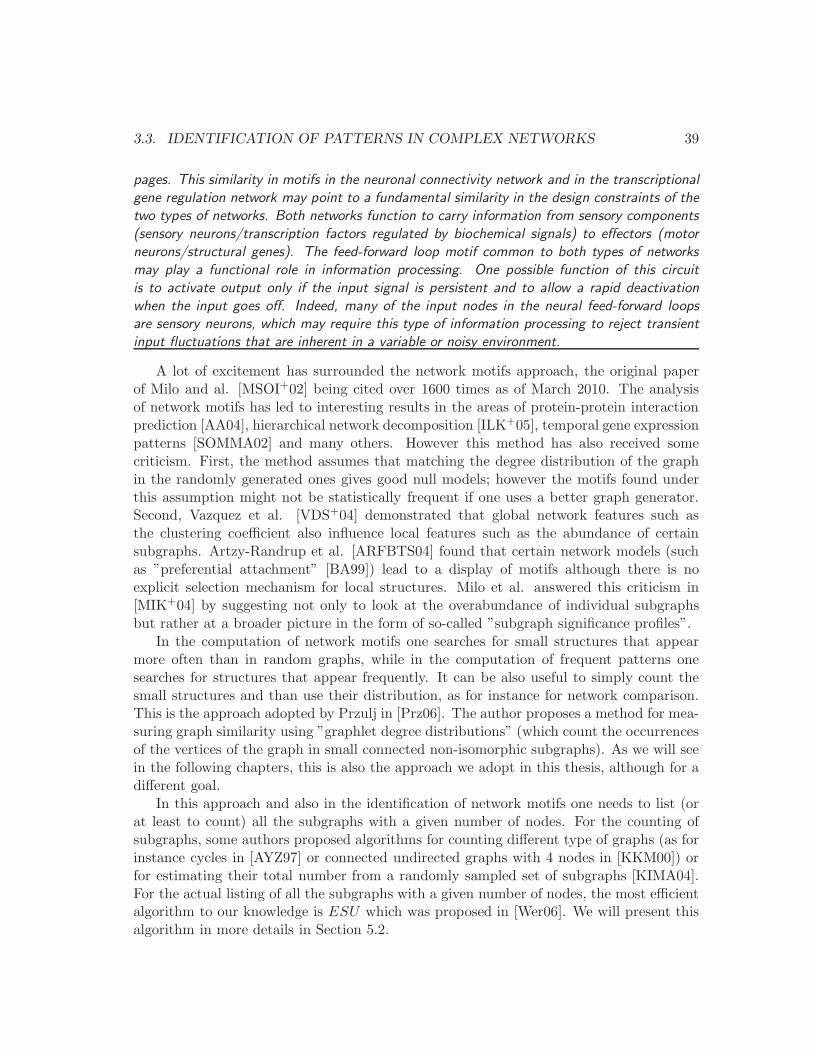
3.3. IDENTIFICATION OF PATTERNS IN COMPLEX NETWORKS 39
pages. This similarity in motifs in the neuronal connectivity network and in the transcriptionalgene regulation network may point to a fundamental similarity in the design constraints of thetwo types of networks. Both networks function to carry information from sensory components(sensory neurons/transcription factors regulated by biochemical signals) to effectors (motorneurons/structural genes). The feed-forward loop motif common to both types of networksmay play a functional role in information processing. One possible function of this circuitis to activate output only if the input signal is persistent and to allow a rapid deactivationwhen the input goes off. Indeed, many of the input nodes in the neural feed-forward loopsare sensory neurons, which may require this type of information processing to reject transientinput fluctuations that are inherent in a variable or noisy environment.
A lot of excitement has surrounded the network motifs approach, the original paperof Milo and al. [MSOI+02] being cited over 1600 times as of March 2010. The analysisof network motifs has led to interesting results in the areas of protein-protein interactionprediction [AA04], hierarchical network decomposition [ILK+05], temporal gene expressionpatterns [SOMMA02] and many others. However this method has also received somecriticism. First, the method assumes that matching the degree distribution of the graphin the randomly generated ones gives good null models; however the motifs found underthis assumption might not be statistically frequent if one uses a better graph generator.Second, Vazquez et al. [VDS+04] demonstrated that global network features such asthe clustering coefficient also influence local features such as the abundance of certainsubgraphs. Artzy-Randrup et al. [ARFBTS04] found that certain network models (suchas ”preferential attachment” [BA99]) lead to a display of motifs although there is noexplicit selection mechanism for local structures. Milo et al. answered this criticism in[MIK+04] by suggesting not only to look at the overabundance of individual subgraphsbut rather at a broader picture in the form of so-called ”subgraph significance profiles”.
In the computation of network motifs one searches for small structures that appearmore often than in random graphs, while in the computation of frequent patterns onesearches for structures that appear frequently. It can be also useful to simply count thesmall structures and than use their distribution, as for instance for network comparison.This is the approach adopted by Przulj in [Prz06]. The author proposes a method for mea-suring graph similarity using ”graphlet degree distributions” (which count the occurrencesof the vertices of the graph in small connected non-isomorphic subgraphs). As we will seein the following chapters, this is also the approach we adopt in this thesis, although for adifferent goal.
In this approach and also in the identification of network motifs one needs to list (orat least to count) all the subgraphs with a given number of nodes. For the counting ofsubgraphs, some authors proposed algorithms for counting different type of graphs (as forinstance cycles in [AYZ97] or connected undirected graphs with 4 nodes in [KKM00]) orfor estimating their total number from a randomly sampled set of subgraphs [KIMA04].For the actual listing of all the subgraphs with a given number of nodes, the most efficientalgorithm to our knowledge is ESU which was proposed in [Wer06]. We will present thisalgorithm in more details in Section 5.2.
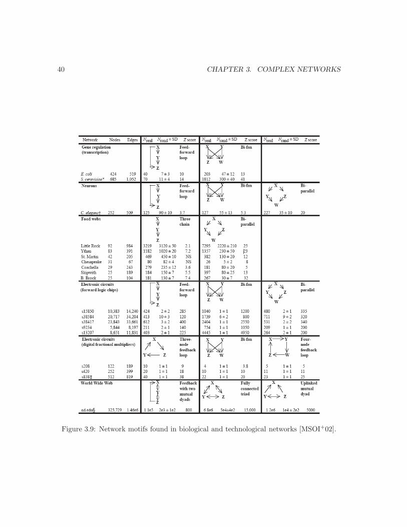
40 CHAPTER 3. COMPLEX NETWORKS
Figure 3.9: Network motifs found in biological and technological networks [MSOI+02].
Chapter 4
Social networks
A social network is a modeling of a set of relations among a set of individuals. It canbe seen as a graph where the vertices are the individuals and the edges are the relationsbetween them. Traditionally, this has been a domain of study for sociologists and anthro-pologists who analyze the connection between individuals or collective behaviors and thesocial structures in which individuals are embedded. The idea of ”social network” hasbeen used for over a century, Georg Simmel being the first scholar to think directly insocial network terms at the beginning of the twentieth century [Sim55a] (English version).His essays pointed to the nature of network size on interaction and to the likelihood ofinteraction in ramified, loosely-knit networks rather than groups. In the 1930s, JacobL. Moreno pioneered the systematic recording and analysis of social interaction in smallgroups, especially classrooms and work groups. In 1954, John A. Barnes [Bar54] startedusing the term ”social network” systematically to denote patterns of ties, encompassingconcepts traditionally used by the public and those used by social scientists: boundedgroups (e.g., tribes, families) and social categories (e.g., gender, ethnicity). The field de-veloped with the works of Elisabeth Bott on kinship [Bot57], of Sigfried Nadel on socialstructure [Nad57], of Harrison White and his students at Harvard University and manyothers. For instance Mark Granovetter and Barry Wellman (whose principal works willbe presented in the following sections) are among the former students of White who haveelaborated and popularized social network analysis.
Generally, the analysis of the structure of interpersonal relations can offer insightsabout the persons’ sociability and can explain their actions. For this type of analysis,sociologists and anthropologists usually obtain their data from interviews with the ana-lyzed people. This data, although very detailed, can be difficult to obtain. The process ofinterviewing people is often long and costly and the obtained datasets rather small, withseveral hundreds of analyzed relations in the best of cases.
Recently, new sources of data have been used. With the development of internet,mobile communication, computer capacity, one can easily access traces of interpersonalcommunication such as activity on online platforms, phone calls, emails, instant messagesetc. The obtained datasets are large, possibly containing millions of communications. Theaccess to data is much easier than before but the obtained sets are less detailed as one sees
41
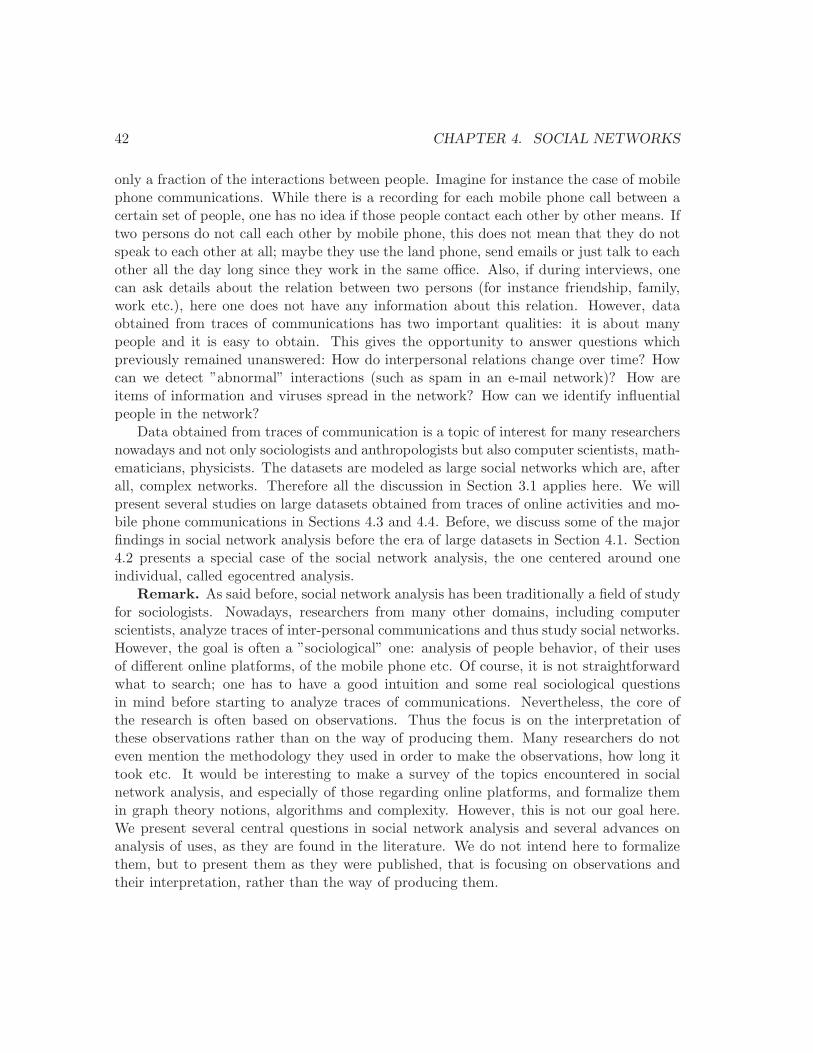
42 CHAPTER 4. SOCIAL NETWORKS
only a fraction of the interactions between people. Imagine for instance the case of mobilephone communications. While there is a recording for each mobile phone call between acertain set of people, one has no idea if those people contact each other by other means. Iftwo persons do not call each other by mobile phone, this does not mean that they do notspeak to each other at all; maybe they use the land phone, send emails or just talk to eachother all the day long since they work in the same office. Also, if during interviews, onecan ask details about the relation between two persons (for instance friendship, family,work etc.), here one does not have any information about this relation. However, dataobtained from traces of communications has two important qualities: it is about manypeople and it is easy to obtain. This gives the opportunity to answer questions whichpreviously remained unanswered: How do interpersonal relations change over time? Howcan we detect ”abnormal” interactions (such as spam in an e-mail network)? How areitems of information and viruses spread in the network? How can we identify influentialpeople in the network?
Data obtained from traces of communication is a topic of interest for many researchersnowadays and not only sociologists and anthropologists but also computer scientists, math-ematicians, physicists. The datasets are modeled as large social networks which are, afterall, complex networks. Therefore all the discussion in Section 3.1 applies here. We willpresent several studies on large datasets obtained from traces of online activities and mo-bile phone communications in Sections 4.3 and 4.4. Before, we discuss some of the majorfindings in social network analysis before the era of large datasets in Section 4.1. Section4.2 presents a special case of the social network analysis, the one centered around oneindividual, called egocentred analysis.
Remark. As said before, social network analysis has been traditionally a field of studyfor sociologists. Nowadays, researchers from many other domains, including computerscientists, analyze traces of inter-personal communications and thus study social networks.However, the goal is often a ”sociological” one: analysis of people behavior, of their usesof different online platforms, of the mobile phone etc. Of course, it is not straightforwardwhat to search; one has to have a good intuition and some real sociological questionsin mind before starting to analyze traces of communications. Nevertheless, the core ofthe research is often based on observations. Thus the focus is on the interpretation ofthese observations rather than on the way of producing them. Many researchers do noteven mention the methodology they used in order to make the observations, how long ittook etc. It would be interesting to make a survey of the topics encountered in socialnetwork analysis, and especially of those regarding online platforms, and formalize themin graph theory notions, algorithms and complexity. However, this is not our goal here.We present several central questions in social network analysis and several advances onanalysis of uses, as they are found in the literature. We do not intend here to formalizethem, but to present them as they were published, that is focusing on observations andtheir interpretation, rather than the way of producing them.
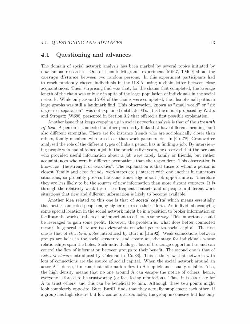
4.1. QUESTIONING AND ADVANCES 43
4.1 Questioning and advances
The domain of social network analysis has been marked by several topics initiated bynow-famous researches. One of them is Milgram’s experiment [Mil67, TM69] about theaverage distance between two random persons. In this experiment participants hadto reach randomly chosen individuals in the U.S.A. using a chain letter between closeacquaintances. Their surprising find was that, for the chains that completed, the averagelength of the chain was only six in spite of the large population of individuals in the socialnetwork. While only around 29% of the chains were completed, the idea of small paths inlarge graphs was still a landmark find. This observation, known as ”small world” or ”sixdegrees of separation”, was not explained until late 90’s. It is the model proposed by Wattsand Strogatz [WS98] presented in Section 3.2 that offered a first possible explanation.
Another issue that keeps cropping up in social networks analysis is that of the strengthof ties. A person is connected to other persons by links that have different meanings andalso different strengths. There are for instance friends who are sociologically closer thanothers, family members who are closer than work partners etc. In [Gra78], Granovetteranalyzed the role of the different types of links a person has in finding a job. By interview-ing people who had obtained a job in the previous five years, he observed that the personswho provided useful information about a job were rarely family or friends, but ratheracquaintances who were in different occupations than the respondent. This observation isknown as ”the strength of weak ties”. The explanation is that those to whom a person isclosest (family and close friends, workmates etc.) interact with one another in numeroussituations, so probably possess the same knowledge about job opportunities. Thereforethey are less likely to be the sources of new information than more distant contacts. It isthrough the relatively weak ties of less frequent contacts and of people in different worksituations that new and different information is likely to become available.
Another idea related to this one is that of social capital which means essentiallythat better connected people enjoy higher return on their efforts. An individual occupyingsome special location in the social network might be in a position to broker information orfacilitate the work of others or be important to others in some way. This importance couldbe leveraged to gain some profit. However, the problem is: what does better connectedmean? In general, there are two viewpoints on what generates social capital. The firstone is that of structural holes introduced by Burt in [Bur92]. Weak connections betweengroups are holes in the social structure, and create an advantage for individuals whoserelationships span the holes. Such individuals get lots of brokerage opportunities and cancontrol the flow of information between groups to their benefit. The second one is that ofnetwork closure introduced by Coleman in [Col88]. This is the view that networks withlots of connections are the source of social capital. When the social network around anactor A is dense, it means that information flow to A is quick and usually reliable. Also,the high density means that no one around A can escape the notice of others; hence,everyone is forced to be trustworthy (or face losing reputation). Thus, it is less risky forA to trust others, and this can be beneficial to him. Although these two points mightlook completely opposite, Burt [Bur01] finds that they actually supplement each other. Ifa group has high closure but low contacts across holes, the group is cohesive but has only
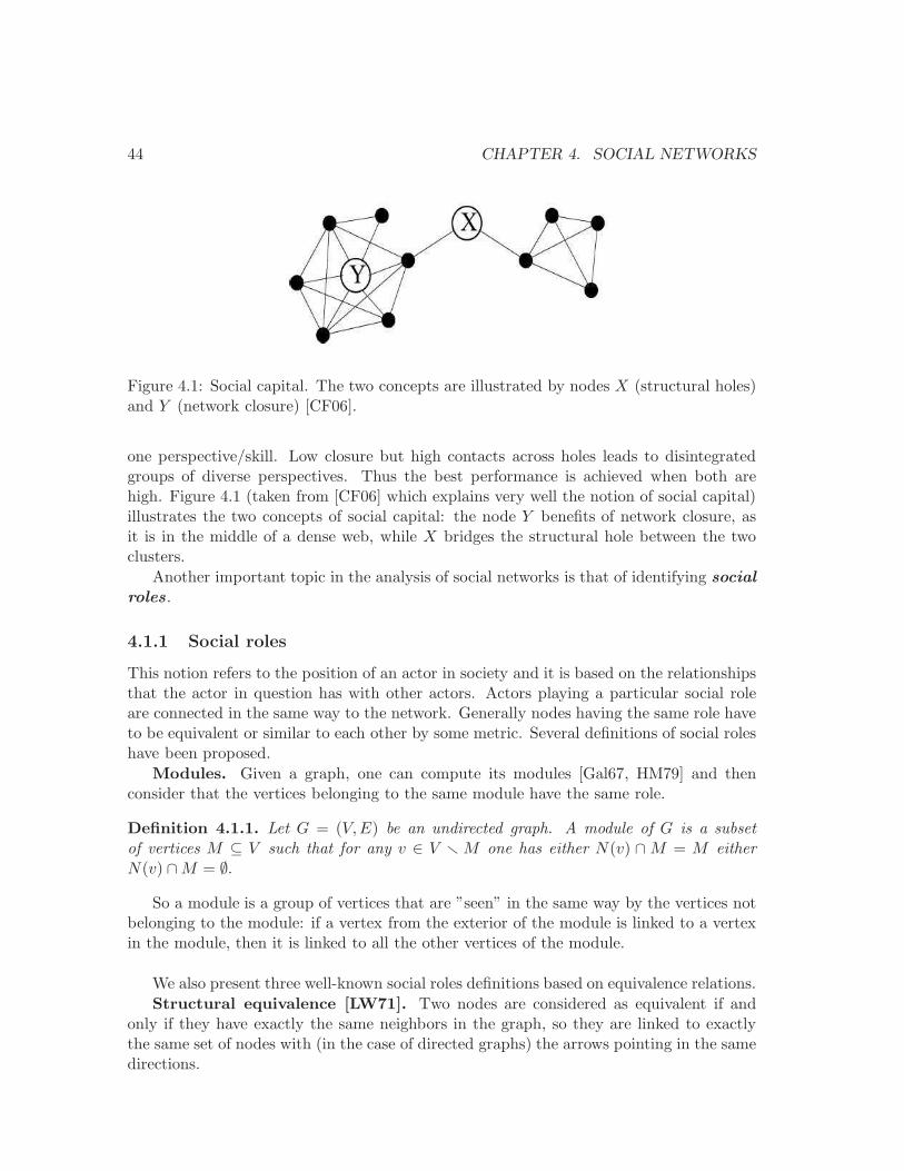
44 CHAPTER 4. SOCIAL NETWORKS
Figure 4.1: Social capital. The two concepts are illustrated by nodes X (structural holes)and Y (network closure) [CF06].
one perspective/skill. Low closure but high contacts across holes leads to disintegratedgroups of diverse perspectives. Thus the best performance is achieved when both arehigh. Figure 4.1 (taken from [CF06] which explains very well the notion of social capital)illustrates the two concepts of social capital: the node Y benefits of network closure, asit is in the middle of a dense web, while X bridges the structural hole between the twoclusters.
Another important topic in the analysis of social networks is that of identifying socialroles.
4.1.1 Social roles
This notion refers to the position of an actor in society and it is based on the relationshipsthat the actor in question has with other actors. Actors playing a particular social roleare connected in the same way to the network. Generally nodes having the same role haveto be equivalent or similar to each other by some metric. Several definitions of social roleshave been proposed.
Modules. Given a graph, one can compute its modules [Gal67, HM79] and thenconsider that the vertices belonging to the same module have the same role.
Definition 4.1.1. Let G = (V,E) be an undirected graph. A module of G is a subsetof vertices M ⊆ V such that for any v ∈ V r M one has either N(v) ∩M = M eitherN(v) ∩M = ∅.
So a module is a group of vertices that are ”seen” in the same way by the vertices notbelonging to the module: if a vertex from the exterior of the module is linked to a vertexin the module, then it is linked to all the other vertices of the module.
We also present three well-known social roles definitions based on equivalence relations.
Structural equivalence [LW71]. Two nodes are considered as equivalent if andonly if they have exactly the same neighbors in the graph, so they are linked to exactlythe same set of nodes with (in the case of directed graphs) the arrows pointing in the samedirections.
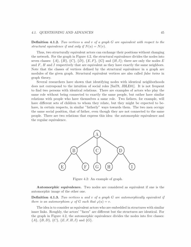
4.1. QUESTIONING AND ADVANCES 45
Definition 4.1.2. Two vertices u and v of a graph G are equivalent with respect to thestructural equivalence if and only if N(u) = N(v).
Thus, two structurally equivalent actors can exchange their positions without changingthe network. For the graph in Figure 4.2, the structural equivalence divides the nodes intoseven classes: {A}, {B}, {C}, {D}, {E,F}, {G} and {H, I}; there are only the nodes Eand F , H and I respectively that are equivalent as they have exactly the same neighbors.Note that the classes of vertices defined by the structural equivalence in a graph aremodules of the given graph. Structural equivalent vertices are also called false twins ingraph theory.
Several researchers have shown that identifying nodes with identical neighborhoodsdoes not correspond to the intuition of social roles [Sai78, JBLE01]. It is not frequentto find two persons with identical relations. There are examples of actors who play thesame role without being connected to exactly the same people, but rather have similarrelations with people who have themselves a same role. Two fathers, for example, willhave different sets of children to whom they relate, but they might be expected to be-have, in certain respects, in similar ”fatherly” ways towards them. The two men occupythe same social position, that of father, even though they are not connected to the samepeople. There are two relations that express this idea: the automorphic equivalence andthe regular equivalence.
Figure 4.2: An example of graph.
Automorphic equivalence. Two nodes are considered as equivalent if one is theautomorphic image of the other one.
Definition 4.1.3. Two vertices u and v of a graph G are automorphically equivalent ifthere is an automorphism ϕ of G such that ϕ(u) = v.
The idea is to consider as equivalent actors who are embedded in structures with similarinner links. Roughly, the actors’ ”faces” are different but the structures are identical. Forthe graph in Figure 4.2, the automorphic equivalence divides the nodes into five classes:{A}, {B,D}, {C}, {E,F,H, I} and {G}.
46 CHAPTER 4. SOCIAL NETWORKS
Regular equivalence [BE89]. Two nodes are considered as equivalent if they areconnected to equivalent nodes.
Definition 4.1.4. Given a graph G = (V,E), let r : V → N be a role assignment for thevertices in V ; the function r can be seen as an attribution of colors to the vertices in V.Also the function r defines an equivalence relation on the vertices in V. This relation issaid to be regular if and only if for all u, v ∈ V such that r(u) = r(v) one has
{r(i); i ∈ N(u)} = {r(i); i ∈ N(v)}
So if two nodes are equivalent, the colors found in the neighborhood of one node arealso found (possibly in different numbers) in the neighborhood of the other node. Forthe graph in Figure 4.2 one possible regular equivalence is that with the following classes:{A}, {B,C,D} and {E,F,G,H, I}, so there are 3 colors: one for the vertex A, anotherone for the vertices B, C and D and another one for the vertices E, F, G, H and I.
Note that this definition is circular: to check if two vertices u and v are equivalent,one has to check if their neighbors are equivalent, and therefore if u and v are equivalent.Algorithms for computing regular equivalences have been proposed for instance in [EB93].
The three definitions presented here are often too strict for real-world data. Theproblem is that only few nodes are found as equivalent when using these definitions onreal-world graphs. Thus the equivalence classes are much too numerous, often of the sameorder of magnitude as the number of vertices of the graph. The idea behind social roles ishowever to group nodes in a small number of clusters that can be easily used. Thereforeone generally uses different heuristics like the computation of a distance between nodes:equivalent nodes are at distance 0 from each other and similar nodes are at a small dis-tance. This distance can be defined for instance as a certain correlation coefficient orsimilarity measure between nodes. Or it can be defined using vectors characterizing thenodes; the distance between the nodes is then the (e.g. Euclidian) distance between theirvectors. After having defined a certain distance between nodes one can use a clusteringalgorithm (as presented in Section 2.2) in order to group nodes into clusters: nodes in thesame cluster are close to each other with respect to the given distance. The advantage isthat one can place the number of clusters where he wants, going from a small number ofclusters (if this is his goal) to a large number of clusters, where nodes in the same clusterare very similar to each other.
We presented here only some of the topics of social network analysis. For a review ofsocial network methods see for instance [WF94].
4.2 Egocentred analysis
In the analysis of social networks, a special part is that of the study of personal relationsi.e. the different relations a given individual (called ego) has with other individuals (oftencalled alters). This is called an egocentred approach because the social relations are seenfrom ego’s point of view. The analyzed relations are generally obtained by interviews
4.2. EGOCENTRED ANALYSIS 47
with ego who describes his relations with the other persons and, sometimes, the relationsbetween these persons. Thus, ego is asked about the people he knows, with whom heinteracts, about the importance of these people in his life etc. One problem here is thetype of questions to ask ego (for instance he is asked to cite the persons he knows, but whatdoes ”know” mean?); this is very important since the recorded data depends entirely on it.This becomes even more complicated when ego is asked to cite the relations between hisalters, as he may have a wrong impression about these relations. The advantage, however,is that the interviewer can ask whatever questions he wants, thus obtaining very detailedand meaningful data.
While the analysis of ego’s relation has a long history in anthropology and sociology[RB40, Bar54, Sim55a, Bot57, Mit69, Boi74], the approach is not always a social networkone in the sense that the structure of the network is not studied; rather, a given relationbetween two persons is analyzed in the context of the existence of other relations. Thus,the focus is predominantly on the different properties of the two individuals and of theirindividual relationships and not on the notion of network as structured configuration. Suchanalysis has been done for instance on romantic relationships [Sur88, PSE83, SEE92] oron the notion of social support [MCN97, BCP02, ATSK04].
In order to analyze personal networks using a social network approach, one needs todefine ego’s network (also called egocentred or personal network or personal community).One has to define a network (or a graph) so a set of nodes and a set of links. The nodesare usually ego and his alters but one can also consider their alters (so the nodes two stepsaway from ego) etc. The presence of the different people is mentioned by ego during theinterviews. For the links, there is a link between ego and each one of his alters. The linksbetween alters, if present, are also given by ego.
Once one has built such an egocentred network, one can study its structure: the numberof nodes, links, the density, the clustering coefficient etc. The analysis of the differentpatterns occurring in people’s personal networks is important because it can show howdifferent networks are structured and why, what part different social and personal factors(e.g. gender, age, mobility histories, ethnicity, profession) play in this, how a person issocially integrated etc.
One of the most influential network analysts from a personal relationship perspective,Barry Wellman, consistently argued that a network approach is fundamental to under-standing the character of contemporary society and the role the personal relations playwithin this. In a series of reports based on data collected from East York, a suburbof Toronto, in the 1970s [Wel79, Wel82, Wel85, WW90], Wellman has been particularlyconcerned with the ways individuals are integrated in social life. In [Wel82, Wel88] hedistinguishes several configurations of relations in terms of network structure: people em-bedded in quite dense networks, people having several subsets of alters and also peoplewhere alters have little to do with each other. In France, egocentred analysis has beenmade popular by Maurizio Gribaudi who introduced the methodology of notebooks of con-tacts [Gri98], Michel Grossetti who studied social structures of personal relations in theToulouse area [Gro05], Dominique Cardon and Fabien Granjon who analyzed the relationbetween cultural practices (media-related, recreational, communication etc.) and personalnetworks structure [CG05], and many others.
48 CHAPTER 4. SOCIAL NETWORKS
If in the studies presented in this section the data came from interviews, in the followingones the data comes from traces of phone communications and online activities.
4.3 Phone communications
We present here an overview of existing studies on large social networks extracted fromtwo different environments: phone communications and online activities.
Several researchers analyzed the phone usage, the way people communicate by mobileor fixed phone in terms of duration or frequency of calls, depending on the sociological orgeographical distance between people, on their gender etc.
In [SL00] Licoppe and Smoreda studied the relationship between the duration of fixedphone calls and the gender of the two persons in communication. The authors used telephonebilling records on several hundreds of adult men and women during 4 months. The analysisshowed that the duration of calls is correlated with receiver’s gender and it is in averagelonger when a woman is called. Also, their in-depth conversation analysis suggested thatpoliteness rules governing the telephone call can explain in part why it is the gender of thereceiver that has the biggest effect on how the call is managed and on its overall duration. Theconversations involving women tended to go through longer introductive sequences, to be moremulti-thematic and digressive in nature with a corresponding lengthening and multiplication ofclosure sequences; meanwhile the conversations with men tend to be linear and monothematic.In the main, the callers seem to adjust their interaction style to the gender of the receiver.
The same authors analyzed the relationship between the intensity of calls and thedistance between the two persons.
In [LS05] Licoppe and Smoreda, using phone calls databases and interviews focusing onthe use of telephone, identified two patterns of communication: the ”connected presence” andthe ”intermittent presence”. In the first pattern of communication, the ”connected presence”,the two persons, socially and often also geographically close, are frequently in contact witheach other, exchanging many short calls and messages. They share activities that requirenumerous calls for synchronization and coordination. In the second pattern, the ”intermittentpresence”, the two persons, close friends or intimate relatives, are not able to see each other ortalk very often. Their conversations are long, they give and receive news, trying to compensatefor the rarity of face-to-face contacts.
These analyses have been done using fixed phone data. Nowadays, the development ofmobile phones and their worldwide spread (a penetration larger than 40% worldwide andclose to 100% in the developed countries) offer new possibilities of analysis. The mobilephone, a individual and ubiquitous device offering voice and text communication features,has transformed the frequency and the geography of communication as compared to olderfixed phone practices. We are now virtually always accessible to others wherever we are.This offers a useful insight into individual behavior. Of course, cellular phone communica-tions do not fully capture social exchange. A social relation is expressed through multipleinteraction channels such as email, land phone communications, instant messaging, face
4.3. PHONE COMMUNICATIONS 49
to face interactions, the mobile phone communications capturing only a subset of the un-derlying social network. However, studies on the strength of ties have shown that mobilephone is among the most intimate communication tools; a mobile phone conversation sug-gests a certain relation between the two individuals, given that there aren’t any listings ofmobile phone numbers. Moreover, people that contact each other via one communicationtool tend to communicate via other ones as well [Hay05], hence the relevance of analyz-ing mobile phone communications in the search of understanding the underlying socialnetwork.
Behavioral data coming from telecommunication operators offers the opportunity torevisit some older research on telephone usages. For instance, using mobile phone com-munication data, Lambiotte et al. [LBdK+08] were able to test the hypothesis that theexistence of a call between two persons depends on the geographical distance betweenthem. They thus show that the probability of a mobile phone call is inversely propor-tional to the square of the geographical distance between the two persons.
Also, new types of analysis are possible. For instance, one can use the location ofthe mobile phone when the communication began (also possibly when it ended) in orderto study people mobility patters. Extensive call records of any mobile phone carriercontain even more detailed information on the spatiotemporal localization of millions ofusers. This is due to the fact that mobile phones, in order to place outgoing calls andto receive incoming calls, must periodically report their presence to nearby cell towers,thus registering their position in the geographical cell covered by one of the towers. Theanalysis of such information for a better understanding of people mobility could be ofhigh interest for urban planning, public transportation design, traffic engineering, diseaseoutbreak control and disaster management. Several studies try to discover the patterns ofmobile phone users mobility [BDE09, GHB08, EP05] and to predict their trajectory. Inthis direction, Song et al. [SQBB10] measure the entropy of each individual’s trajectory,thus finding a high potential predictability in user mobility.
Mobile phone communications have also been modeled as complex social networks andanalyzed accordingly. In several studies the nodes of the modeling graph are the individualscommunicating by mobile phone during a given period, while the links correspond toreciprocal communications: two nodes are connected by a link if there had been a leastone communication between the two persons in each direction (i.e. A called B and Bcalled A). This procedure eliminates one-way calls that suggest that the caller does notknow the receiver personally.
In this approach, Onnela et al. [OSH+07b] used a graph modeling mobile phone commu-nications where they computed the degree distribution. As expected, most users communicatewith only a few individuals while a small minority talks with dozens. However, the degreedistribution decays very fast, so the hubs (high-degree nodes) are few; this is different fromthe case of land lines and of emails where well-connected hubs are present. This situation isprobably rooted in the fact that institutional phone numbers, corresponding to the vast major-ity of large hubs in the case of land lines, are absent, and in contrast with e-mail, in which asingle e-mail can be sent to many recipients, resulting in well-connected hubs, a mobile phoneconversation typically represents a one-to-one communication. The authors define the weight
50 CHAPTER 4. SOCIAL NETWORKS
of a link (its strength) as the total duration of mobile phone communications between the twopersons; they study the relationship between the strength of ties and their betweenness central-ity, finding that the two are negatively correlated. Next, the authors analyze the importance oflinks of different strength for the robustness of the network (actually of the largest connectedcomponent that contains 84% of the nodes). They thus find that the removal of the weak tiesleads to a sudden, phase transition-driven collapse of the whole network. In contrast, the re-moval of the strong ties results only in the network’s gradual shrinking but not its collapse. Bysimulating information diffusion in the network, they find that the process of diffusion changesdramatically when the strength of links is taken into consideration (as opposed to the situationwhere all the links are considered as having equal weight). Moreover, in contrast with thetheory of the importance of weak ties in information access [Gra78], they find that both weakand strong ties have a relatively insignificant role as conduits for information (”the weakness ofweak and strong ties”): the former because the small amount of on-air time offers little chanceof information transfer and the latter because they are mostly confined within communities,with little access to new information. They finally conjecture that communication networksare better suited to local information processing than global information transfer.
The same authors develop the analysis of links weight in [OSH+07a] in mobile phonecommunications networks.
In [OSH+07a] Onnela et al. take into consideration both the duration of calls andthe total number of calls between the two persons as weight of the link connecting them.Besides computing classical measures, such as different distributions, the authors define theintensity of a subgraph as the geometrical mean of the weights of its links. They count thenumber of fully connected subgraphs (i.e. cliques) with 2 to 10 vertices in their network andin randomly generated Erdos-Renyi networks, finding that cliques with more than 3 verticesappear a enormous number of times more often in the real graph than in the generated ones.Note, however, that it had already been observed that the number of triangles was a lot higherin real-world complex networks than in Erdos-Renyi graph, so the authors’ conclusion is notsurprising. When comparing the intensity of subgraphs in the real network and in a networkwhere the links weight have been shuffled, the authors find that the real-world subgraphs haveconsiderably higher intensities than the random ones. This shows that local organization ofweights in the mobile phone graph is not random.
Several researchers analyzed the temporal dynamics of mobile phone networks e.g. thetemporal stability of links. In [HRS08], Hidalgo and Rodriguez-Sickert define the per-sistence of a link over a set of time periods as the number of periods where the link isactivated (there are reciprocal calls between the two persons during that period). Theyfind that persistent links are more common with people with low degree and high cluster-ing. Palla, Barabasi and Vicsek [PBV07] used mobile phone data to study the evolutionof social groups. They found that large groups persist for longer times if they are ca-pable of dynamically altering their membership, suggesting that an ability to change thegroup composition results in better adaptability. In contrast, the behavior of small groupsdisplays the opposite tendency, the condition for long-term persistence being that theircomposition remains stable.
4.4. ONLINE ACTIVITIES 51
4.4 Online activities
Nowadays, the development of Web2.0 allows users to connect to platforms of social net-working, sharing of photos, videos, blogging, where they interact, declare friendship re-lations and share contents, thus being active participants and not only simple visitors ofsites. In this context, new digital practices have emerged for production and diffusion ofcontents and also for recommendation, tagging and social networking. Moreover each useris able to manage his own visibility and, throughout his profile, develop strategies for in-creasing the audience of his productions and therefore his popularity. Thanks to more andmore precise tracking tools, he knows how many people viewed, commented, recommended,rated, and forwarded his work. These ratings, by increasing the users reflexivity abouthis popularity, strongly influence publishing and networking practices [Hal08], [HRW08],leading some authors to describe the Web as a huge space of competition for popularity[Waz09].
The analysis of usages and contents on these online platforms should help us anticipateusers’ expectations, develop recommendation systems, strengthen contents audience andgrowing of communities, improve segmentation and targeting of users.
Generally, one can adopt one of the three following approaches to analyze activity ononline platforms:
1. analysis of usages (the way users act on these platforms),
2. analysis of the published contents (audience, diffusion etc),
3. analysis of the social networks that model the relations between individuals.
1 Usages. People connect and use the functionalities of online platforms in differentways, often with uneven frequencies (”burtsy nature”). Generally, to measure users’ activ-ity, one looks at the traces left on the platforms, such as number of comments a user writes,number of photos he uploads etc. The different measures of activity are found to have askewed distribution on news groups [FSW06], wikis [HBB07], online dating communities[HEL04], question answer forms [ZAA07, AZBA08].
In [GH06] Golder and Huberman analyze user activity on Del.icio.us, a site for recordingbookmarks. Users can store bookmarks of webpages, in the same way as in browsers but withaccess from any computer, and can tag them with keywords. Delicious is considered ”social”because, not only can one see his own bookmarks, one can also see all of every other usersbookmarks. By analyzing two sets of Delicious data containing almost 20 thousand bookmarks,the authors observe that users vary greatly in the frequency and nature of their Delicious use.That is, some users use Delicious very frequently, and others less frequently. Also some usershave large sets of tags, others have small sets, and there is very little correlation between thenumber of bookmarks a user stores and the number of tags he uses. Users’ tag lists grow overtime, as they discover new interests and add new tags to categorize and describe them, butthe growth rates may be very different. The authors also identify different function of tags.Although a significant amount of tagging, if not all, is done for personal use rather than public
52 CHAPTER 4. SOCIAL NETWORKS
benefit, information tagged for personal use can benefit other users. In this way, Deliciousfunctions as a recommendation system, even without explicitly providing recommendations.
When analyzing the way people make use of the functionalities of online platforms,one can for instance identify groups (or clusters) of individuals based on the measures ofactivity, as in [MAA08] for Youtube or [PCB+08] for Flickr users. All in all, the analysisof uses on online platforms gives us an idea of how different functionalities are used andcan thus help developers of such platforms to improve them.
2 Contents. Many studies analyze the contents published on online platforms. Forinstance, some works concentrate on the success of such contents. Understanding thepopularity characteristics is important because it can bring forward the latent demandcreated by bottlenecks in the system (e.g. poor search and recommendation engines,lack of metadata). It also greatly affects the strategies for marketing, target advertising,recommendation, and search engines.
In [CKR+07], the popularity of videos on Youtube (the world’s largest site for publishingof videos), measured as number of views, is found not to be a perfect power-law. In thelog-log plot, the distribution of the number of view is not a straight line at the two ends:the most popular and the least popular items. There are several possible explanations forthis observation that contradicts Anderson’s intuition of a ”long tail” [And06]. For the leastpopular items, that receive fewer views than if the distribution was a straight line on all itslength, it can be because many videos are of low interest to most users; these videos are oftenproduced for small audience e.g. family members. Also, search or recommendation enginestypically return or favor a small number of popular items [CR04, MBSA02], steering usersaway from unpopular ones. This way users cannot easily discover niche content because thiscontent is not properly categorized or ranked. The most popular videos also receive fewer viewsthan if the distribution was a straight line on all its length. A possible explanation, suggestedin [GDS+03] for P2P downloads and adopted in [CKR+07] for Youtube videos, is that videocontent does not change (is immutable); therefore viewers are not likely to watch the samevideo multiple times, as they do for mutable web objects. Even the number of views of verypopular items does not go past a certain limit, so there is a cutoff in the distribution.
As in the Pareto principle (or 80-20 rule), the audience is often concentrated on a minorityof contents: on Youtube 10% of the top popular videos count for nearly 80% of views, while therest 90% of the videos receive very few requests. Besides the argument that recommendationtools and search engine favor popular items, another argument is that users tend to consumethe most popular contents (the hits on home pages, the subjects of buzz, the most seencontents: winner takes it all [Fra95]). As for the evolution of the popularity of Youtube videosin time, the number of views 5, 7 and 90 days after the publication of the video is found to behighly correlated to its popularity after 2 days. So a video with little audience two days afterits apparition on Youtube is likely to rest unpopular forever.
The prediction of audience of contents is also addressed in [SH08], while other authorsidentify different patterns of success (for photos on Flickr [CMG09]) or different types ofcontents based on the attention they are given ([CS08]).
4.4. ONLINE ACTIVITIES 53
The two aspects, uses and contents on online platforms, are often analyzed together.This seems logical as the content is published by users and made popular by their uses.When analyzing the popularity of contents one often analyzes the strategies developed byusers to build the popularity, so the uses of the tools for social networking or promotion.Also, the analysis of uses often raises questions about the success of the published contents.For instance, in the previously evoked study on the uses of tags on Delicious [GH06],the authors analyze also the popularity of URLs measured as the number of bookmarkscontaining them. In another study Huberman et al. [HRW08] show that productivity onYoutube is dependent of the attention received by a content: a lack of attention leads toa decline of the activity.
3 Social networks. Many of the online platforms give users the possibility to linkto other users by explicitly declaring a relation (such as friendship or fan etc.) or byleaving traces on other users’ profiles (such as comments). These relations between userscan be modeled by graphs. The analysis of such graphs is important as it can providecharacterizations of the individuals and of the links between them. For instance, one couldlook for individuals that have similar positions in the graph because these individuals arelikely to act similarly on the platform. Moreover one can characterize individuals byusing endogenous variables of the social network and also exogenous variables (such asage, gender, town, quantity of published content, quantity of comments etc.) and thenmeasure the correlations between the two types of variables. If the two are correlated, onecan predict one using the others which can be very useful if some of the information ishidden.
If data on users of online platforms is generally rich and public (personal data, declaredfriendship relations, comments are public on sites like MySpace, Flickr, Twitter etc.),which is rarely the case for offline data, the analysis of the relations between the users ofan online platform may be difficult. First, for most of the platforms one cannot analyzethe whole set of relations because this set is too big and the recording of the relationstoo long. Therefore one usually builds a sample of the relations present on the platformby doing a breadth-first search aspiration (see Section 2.1 for a presentation of the BFSmethod) of profiles: starting from some initial profiles, one follows a given relation (suchas friendship declaration) and goes from profile to profile, recording the found data. TheBFS crawling produces a sample with a relevant structure (good fitting of the clustering,density, and centrality values) but underestimates the in-degree and overestimates theout-degree [MMG+07], [KNT06]. Second, data is often noisy: many profiles may not beactive (their creators never go on the profile), a user may have several profiles, the relationsmay not correspond to real social relations between individuals (they are artificially andmaybe randomly created), the nature of the relations may be completely hidden (some ofthem correspond to real strong social relations, some other do not have a correspondentin the real life, but all of them have the same form on the platform: they are all friendshiprelations for instance).
Once we have obtained a set of data that can be modeled by a graph, we have a socialnetwork which often is also a complex network, so all the discussion in Chapter 3 applieshere. One can analyze the data at three levels: global, by characterizing the network asa whole, local, by evaluating the local structure of the network, around each node, or
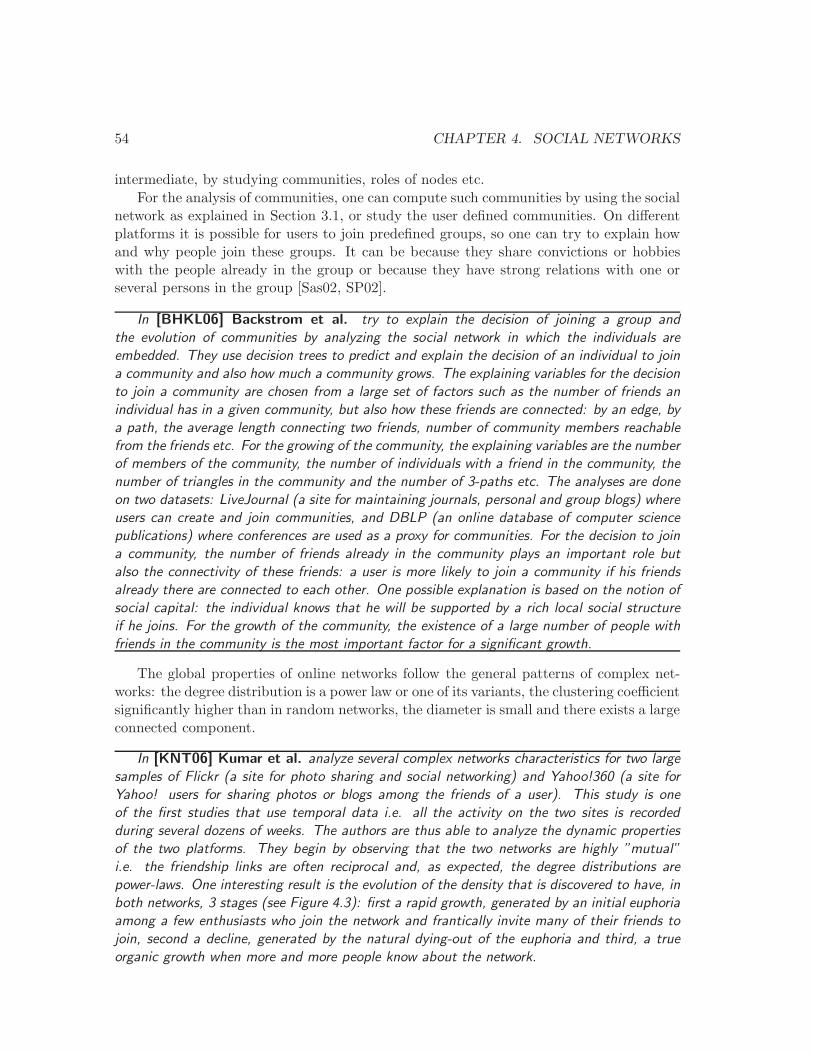
54 CHAPTER 4. SOCIAL NETWORKS
intermediate, by studying communities, roles of nodes etc.
For the analysis of communities, one can compute such communities by using the socialnetwork as explained in Section 3.1, or study the user defined communities. On differentplatforms it is possible for users to join predefined groups, so one can try to explain howand why people join these groups. It can be because they share convictions or hobbieswith the people already in the group or because they have strong relations with one orseveral persons in the group [Sas02, SP02].
In [BHKL06] Backstrom et al. try to explain the decision of joining a group andthe evolution of communities by analyzing the social network in which the individuals areembedded. They use decision trees to predict and explain the decision of an individual to joina community and also how much a community grows. The explaining variables for the decisionto join a community are chosen from a large set of factors such as the number of friends anindividual has in a given community, but also how these friends are connected: by an edge, bya path, the average length connecting two friends, number of community members reachablefrom the friends etc. For the growing of the community, the explaining variables are the numberof members of the community, the number of individuals with a friend in the community, thenumber of triangles in the community and the number of 3-paths etc. The analyses are doneon two datasets: LiveJournal (a site for maintaining journals, personal and group blogs) whereusers can create and join communities, and DBLP (an online database of computer sciencepublications) where conferences are used as a proxy for communities. For the decision to joina community, the number of friends already in the community plays an important role butalso the connectivity of these friends: a user is more likely to join a community if his friendsalready there are connected to each other. One possible explanation is based on the notion ofsocial capital: the individual knows that he will be supported by a rich local social structureif he joins. For the growth of the community, the existence of a large number of people withfriends in the community is the most important factor for a significant growth.
The global properties of online networks follow the general patterns of complex net-works: the degree distribution is a power law or one of its variants, the clustering coefficientsignificantly higher than in random networks, the diameter is small and there exists a largeconnected component.
In [KNT06] Kumar et al. analyze several complex networks characteristics for two largesamples of Flickr (a site for photo sharing and social networking) and Yahoo!360 (a site forYahoo! users for sharing photos or blogs among the friends of a user). This study is oneof the first studies that use temporal data i.e. all the activity on the two sites is recordedduring several dozens of weeks. The authors are thus able to analyze the dynamic propertiesof the two platforms. They begin by observing that the two networks are highly ”mutual”i.e. the friendship links are often reciprocal and, as expected, the degree distributions arepower-laws. One interesting result is the evolution of the density that is discovered to have, inboth networks, 3 stages (see Figure 4.3): first a rapid growth, generated by an initial euphoriaamong a few enthusiasts who join the network and frantically invite many of their friends tojoin, second a decline, generated by the natural dying-out of the euphoria and third, a trueorganic growth when more and more people know about the network.
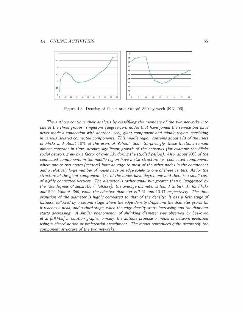
4.4. ONLINE ACTIVITIES 55
Figure 4.3: Density of Flickr and Yahoo! 360 by week [KNT06].
The authors continue their analysis by classifying the members of the two networks intoone of the three groups: singletons (degree-zero nodes that have joined the service but havenever made a connection with another user), giant component and middle region, consistingin various isolated connected components. This middle region contains about 1/3 of the usersof Flickr and about 10% of the users of Yahoo! 360. Surprisingly, these fractions remainalmost constant in time, despite significant growth of the networks (for example the Flickrsocial network grew by a factor of over 13x during the studied period). Also, about 90% of theconnected components in the middle region have a star structure i.e. connected componentswhere one or two nodes (centers) have an edge to most of the other nodes in the componentand a relatively large number of nodes have an edge solely to one of these centers. As for thestructure of the giant component, 1/2 of the nodes have degree one and there is a small coreof highly connected vertices. The diameter is rather small but greater than 6 (suggested bythe ”six-degrees of separation” folklore): the average diameter is found to be 6.01 for Flickrand 8.26 Yahoo! 360, while the effective diameter is 7.61 and 10.47 respectively. The timeevolution of the diameter is highly correlated to that of the density: it has a first stage offlatness, followed by a second stage where the edge density drops and the diameter grows tillit reaches a peak, and a third stage, when the edge density starts increasing and the diameterstarts decreasing. A similar phenomenon of shrinking diameter was observed by Leskovecet al [LKF05] in citation graphs. Finally, the authors propose a model of network evolutionusing a biased notion of preferential attachment. The model reproduces quite accurately thecomponent structure of the two networks.
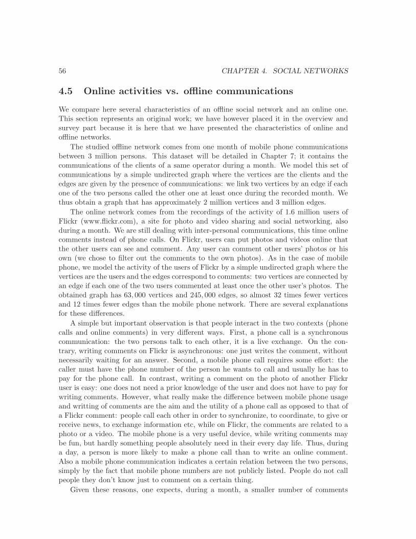
56 CHAPTER 4. SOCIAL NETWORKS
4.5 Online activities vs. offline communications
We compare here several characteristics of an offline social network and an online one.This section represents an original work; we have however placed it in the overview andsurvey part because it is here that we have presented the characteristics of online andoffline networks.
The studied offline network comes from one month of mobile phone communicationsbetween 3 million persons. This dataset will be detailed in Chapter 7; it contains thecommunications of the clients of a same operator during a month. We model this set ofcommunications by a simple undirected graph where the vertices are the clients and theedges are given by the presence of communications: we link two vertices by an edge if eachone of the two persons called the other one at least once during the recorded month. Wethus obtain a graph that has approximately 2 million vertices and 3 million edges.
The online network comes from the recordings of the activity of 1.6 million users ofFlickr (www.flickr.com), a site for photo and video sharing and social networking, alsoduring a month. We are still dealing with inter-personal communications, this time onlinecomments instead of phone calls. On Flickr, users can put photos and videos online thatthe other users can see and comment. Any user can comment other users’ photos or hisown (we chose to filter out the comments to the own photos). As in the case of mobilephone, we model the activity of the users of Flickr by a simple undirected graph where thevertices are the users and the edges correspond to comments: two vertices are connected byan edge if each one of the two users commented at least once the other user’s photos. Theobtained graph has 63, 000 vertices and 245, 000 edges, so almost 32 times fewer verticesand 12 times fewer edges than the mobile phone network. There are several explanationsfor these differences.
A simple but important observation is that people interact in the two contexts (phonecalls and online comments) in very different ways. First, a phone call is a synchronouscommunication: the two persons talk to each other, it is a live exchange. On the con-trary, writing comments on Flickr is asynchronous: one just writes the comment, withoutnecessarily waiting for an answer. Second, a mobile phone call requires some effort: thecaller must have the phone number of the person he wants to call and usually he has topay for the phone call. In contrast, writing a comment on the photo of another Flickruser is easy: one does not need a prior knowledge of the user and does not have to pay forwriting comments. However, what really make the difference between mobile phone usageand writting of comments are the aim and the utility of a phone call as opposed to that ofa Flickr comment: people call each other in order to synchronize, to coordinate, to give orreceive news, to exchange information etc, while on Flickr, the comments are related to aphoto or a video. The mobile phone is a very useful device, while writing comments maybe fun, but hardly something people absolutely need in their every day life. Thus, duringa day, a person is more likely to make a phone call than to write an online comment.Also a mobile phone communication indicates a certain relation between the two persons,simply by the fact that mobile phone numbers are not publicly listed. People do not callpeople they don’t know just to comment on a certain thing.
Given these reasons, one expects, during a month, a smaller number of comments
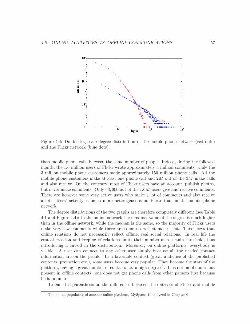
4.5. ONLINE ACTIVITIES VS. OFFLINE COMMUNICATIONS 57
Figure 4.4: Double log scale degree distribution in the mobile phone network (red dots)and the Flickr network (blue dots).
than mobile phone calls between the same number of people. Indeed, during the followedmonth, the 1.6 million users of Flickr wrote approximately 4 million comments, while the3 million mobile phone customers made approximately 150 million phone calls. All themobile phone customers make at least one phone call and 2M out of the 3M make callsand also receive. On the contrary, most of Flickr users have an account, publish photos,but never make comments. Only 63, 000 out of the 1.6M users give and receive comments.There are however some very active users who make a lot of comments and also receivea lot. Users’ activity is much more heterogeneous on Flickr than in the mobile phonenetwork.
The degree distributions of the two graphs are therefore completely different (see Table4.1 and Figure 4.4): in the online network the maximal value of the degree is much higherthan in the offline network, while the median is the same, so the majority of Flickr usersmake very few comments while there are some users that make a lot. This shows thatonline relations do not necessarily reflect offline, real social relations. In real life thecost of creation and keeping of relations limits their number at a certain threshold, thusintroducing a cut-off in the distribution. Moreover, on online platforms, everybody isvisible. A user can connect to any other user simply because all the needed contactinformation are on the profile. In a favorable context (great audience of the publishedcontents, promotion etc.), some users become very popular. They become the stars of theplatform, having a great number of contacts i.e. a high degree 1. This notion of star is notpresent in offline contexts: one does not get phone calls from other persons just becausehe is popular.
To end this parenthesis on the differences between the datasets of Flickr and mobile
1The online popularity of another online platform, MySpace, is analyzed in Chapter 6
58 CHAPTER 4. SOCIAL NETWORKS
Table 4.1: The number of nodes and links of the two networks and their average, maximaland median degree
network # nodes # links avg degree max degree med degree
Flickr 63 × 103 245 × 103 7.8 695 2
mobile phone 2× 10⁶ 3× 10⁶ 3.3 96 2
phone communications, note that we defined the edges of the two graphs in the sameway, by using the existence of communications. Generally one uses for online platformsthe declared links (e.g. friendship links) as edges. However, many declared links are notactive: the users do not contact each other, they have declared each other as friends butthey haven’t had any contact since. Taking into consideration only the links sustained bya certain activity allows us to filter out these cases of unused links.
4.6 Applications: Marketing and services
For a products or services provider, the knowledge of its customers is essential in orderto target the audience, to propose services and publicity adapted to each user etc. Tocharacterize the customers, several dimensions can be taken into consideration: the dif-ferent socio-demographic information (such as age, gender, job, residence etc.), the usescustomers make of the different services, and the social network in which they are embed-ded. The social network dimension is important because people do not live isolated lives,they are surrounded by other people who might influence them.
If marketing models take or not into consideration the social network aspect (althoughit is frequently shown that different parameters computed in the social network improvemarketing models), there is one field of marketing that studies this dimension: the viralmarketing. This field exploits existing social networks by encouraging customers to shareproduct information with their friends. The motivation is that individuals are influencedby their personal relations in the decision of adopting innovations and products (this isalso known as the Word-of-mouth, WOM, influence). Several researches brought this tolight. For instance, sociological studies on individual choice, initiated in the 1940s’ by P.Lazarsfeld team at Bureau of Applied Social Research at Columbia University, emphasizedthe influence of the network of personal relations in the decision of purchase. Engel et al.[EBK69] find that 60% of the persons asked about the choice of a car garage cited theWOM as main influence. Also, Feldman and Spencer [FS65] estimate to two-thirds theratio of new residents of a community who used WOM for finding a doctor. Even studyinstitutes as Harris Interactive [AD07] or BIGresearch tried to measure the importance ofWOM. If the former provided a ranking of products depending on the degree of influenceof WOM in the decision of consumption, the latter state that more than 90% of theinterviewed persons give or receive purchase advice.
In the context of the internet, word-of-mouth advertising is not restricted to pairwiseor small-group interactions between individuals. Rather, customers can share their experi-ences and opinions regarding a product with everyone. Quantitative marketing techniques
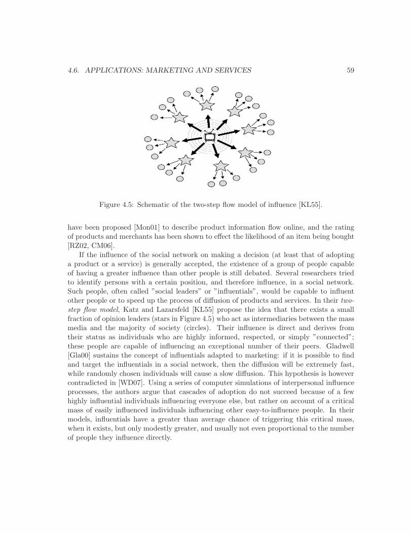
4.6. APPLICATIONS: MARKETING AND SERVICES 59
Figure 4.5: Schematic of the two-step flow model of influence [KL55].
have been proposed [Mon01] to describe product information flow online, and the ratingof products and merchants has been shown to effect the likelihood of an item being bought[RZ02, CM06].
If the influence of the social network on making a decision (at least that of adoptinga product or a service) is generally accepted, the existence of a group of people capableof having a greater influence than other people is still debated. Several researchers triedto identify persons with a certain position, and therefore influence, in a social network.Such people, often called ”social leaders” or ”influentials”, would be capable to influentother people or to speed up the process of diffusion of products and services. In their two-step flow model, Katz and Lazarsfeld [KL55] propose the idea that there exists a smallfraction of opinion leaders (stars in Figure 4.5) who act as intermediaries between the massmedia and the majority of society (circles). Their influence is direct and derives fromtheir status as individuals who are highly informed, respected, or simply ”connected”;these people are capable of influencing an exceptional number of their peers. Gladwell[Gla00] sustains the concept of influentials adapted to marketing: if it is possible to findand target the influentials in a social network, then the diffusion will be extremely fast,while randomly chosen individuals will cause a slow diffusion. This hypothesis is howevercontradicted in [WD07]. Using a series of computer simulations of interpersonal influenceprocesses, the authors argue that cascades of adoption do not succeed because of a fewhighly influential individuals influencing everyone else, but rather on account of a criticalmass of easily influenced individuals influencing other easy-to-influence people. In theirmodels, influentials have a greater than average chance of triggering this critical mass,when it exists, but only modestly greater, and usually not even proportional to the numberof people they influence directly.

60 CHAPTER 4. SOCIAL NETWORKS

Part II
Methods and Applications
61

Chapter 5
A method for analyzing the localstructure of large networks
In this chapter we present a method for analyzing the local structure of a (possibly large)network by characterizing the way each node is connected to the network. The methodis designed to be applied to a given node of a network; in this case it produces a char-acterization of the configuration of the network surrounding the node: the structures inwhich the node it is embedded, the way its neighbors are placed with respect to the othersand the way its links are disposed. One can apply this method to all the nodes of thenetwork, thus obtaining a description of its local structure, or only to some of its nodes:it can be useful if one has only a fraction of the nodes of the network or if the goal isto compare some nodes to each other. Before presenting the method, we introduce someuseful notions. Then we explain the method and we compare the measures produced byit to other existing indicators. We finish this chapter by making some comments on theusefulness of the method.
5.1 Definitions
Unless specified otherwise, all the considered graphs are simple and undirected.
Egocentred network. Given a graph G = (V,E) and a vertex v ∈ V , we callegocentred network of v, denoted by Eg(v), the subgraph induced in G by the neighborsof v i.e. the graph whose vertices are the neighbors of v and whose edges are the edgesbetween these neighbors.
Patterns and positions. We call k-patterns all the non-isomorphic connected graphswith at most k vertices and at least 1 edge. Figure 5.1 presents the thirty 5-patterns. Thereare nine 4-patterns (indices 1 to 9) and three 3-patterns (indices 1 to 3). In this chapterwe consider only 5-patterns that we call simply patterns.
Given a graph, two vertices are said to be position equivalent if there is an adjacencypreserving permutation of the vertices of the graph such that the two vertices are inter-changed (the position equivalence is actually the automorphic equivalence). A position isa maximal set of position equivalent vertices. For example, for each pattern in Figure 5.1,
63
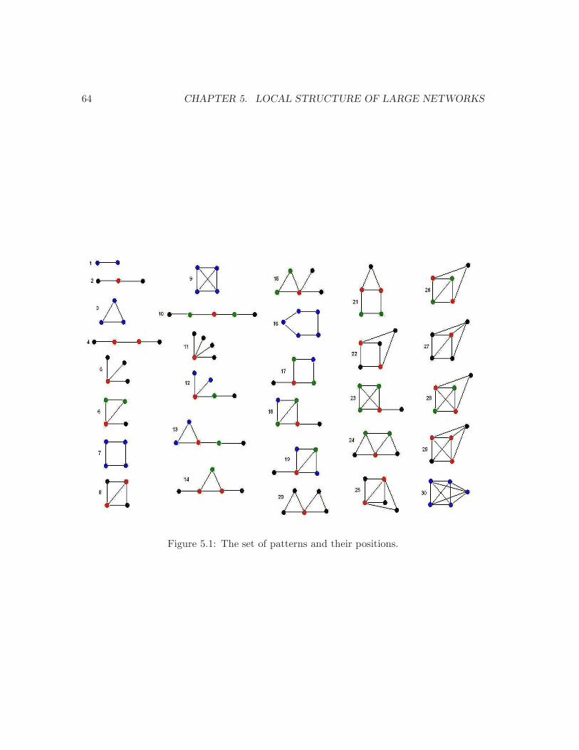
64 CHAPTER 5. LOCAL STRUCTURE OF LARGE NETWORKS
Figure 5.1: The set of patterns and their positions.
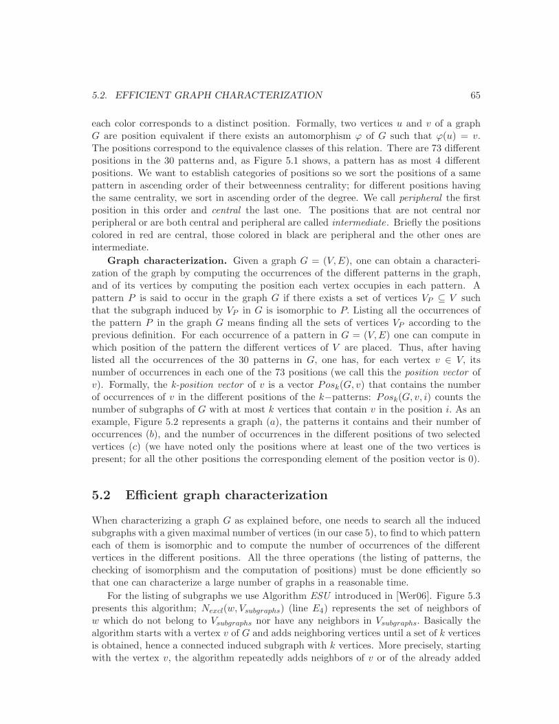
5.2. EFFICIENT GRAPH CHARACTERIZATION 65
each color corresponds to a distinct position. Formally, two vertices u and v of a graphG are position equivalent if there exists an automorphism ϕ of G such that ϕ(u) = v.The positions correspond to the equivalence classes of this relation. There are 73 differentpositions in the 30 patterns and, as Figure 5.1 shows, a pattern has as most 4 differentpositions. We want to establish categories of positions so we sort the positions of a samepattern in ascending order of their betweenness centrality; for different positions havingthe same centrality, we sort in ascending order of the degree. We call peripheral the firstposition in this order and central the last one. The positions that are not central norperipheral or are both central and peripheral are called intermediate. Briefly the positionscolored in red are central, those colored in black are peripheral and the other ones areintermediate.
Graph characterization. Given a graph G = (V,E), one can obtain a characteri-zation of the graph by computing the occurrences of the different patterns in the graph,and of its vertices by computing the position each vertex occupies in each pattern. Apattern P is said to occur in the graph G if there exists a set of vertices VP ⊆ V suchthat the subgraph induced by VP in G is isomorphic to P. Listing all the occurrences ofthe pattern P in the graph G means finding all the sets of vertices VP according to theprevious definition. For each occurrence of a pattern in G = (V,E) one can compute inwhich position of the pattern the different vertices of V are placed. Thus, after havinglisted all the occurrences of the 30 patterns in G, one has, for each vertex v ∈ V, itsnumber of occurrences in each one of the 73 positions (we call this the position vector ofv). Formally, the k-position vector of v is a vector Posk(G, v) that contains the numberof occurrences of v in the different positions of the k−patterns: Posk(G, v, i) counts thenumber of subgraphs of G with at most k vertices that contain v in the position i. As anexample, Figure 5.2 represents a graph (a), the patterns it contains and their number ofoccurrences (b), and the number of occurrences in the different positions of two selectedvertices (c) (we have noted only the positions where at least one of the two vertices ispresent; for all the other positions the corresponding element of the position vector is 0).
5.2 Efficient graph characterization
When characterizing a graph G as explained before, one needs to search all the inducedsubgraphs with a given maximal number of vertices (in our case 5), to find to which patterneach of them is isomorphic and to compute the number of occurrences of the differentvertices in the different positions. All the three operations (the listing of patterns, thechecking of isomorphism and the computation of positions) must be done efficiently sothat one can characterize a large number of graphs in a reasonable time.
For the listing of subgraphs we use Algorithm ESU introduced in [Wer06]. Figure 5.3presents this algorithm; Nexcl(w, Vsubgraphs) (line E4) represents the set of neighbors ofw which do not belong to Vsubgraphs nor have any neighbors in Vsubgraphs. Basically thealgorithm starts with a vertex v of G and adds neighboring vertices until a set of k verticesis obtained, hence a connected induced subgraph with k vertices. More precisely, startingwith the vertex v, the algorithm repeatedly adds neighbors of v or of the already added
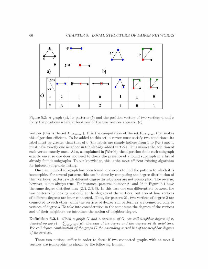
66 CHAPTER 5. LOCAL STRUCTURE OF LARGE NETWORKS
Figure 5.2: A graph (a), its patterns (b) and the position vectors of two vertices u and v(only the positions where at least one of the two vertices appears) (c).
vertices (this is the set Vextension). It is the computation of the set Vextension that makesthis algorithm efficient. To be added to this set, a vertex must satisfy two conditions: itslabel must be greater than that of v (the labels are simply indices from 1 to |VG|) and itmust have exactly one neighbor in the already added vertices. This insures the addition ofeach vertex exactly once. Also, as explained in [Wer06], the algorithm finds each subgraphexactly once, so one does not need to check the presence of a found subgraph in a list ofalready founds subgraphs. To our knowledge, this is the most efficient existing algorithmfor induced subgraphs listing.
Once an induced subgraph has been found, one needs to find the pattern to which it isisomorphic. For several patterns this can be done by computing the degree distribution oftheir vertices: patterns with different degree distributions are not isomorphic. The reverse,however, is not always true. For instance, patterns number 21 and 22 in Figure 5.1 havethe same degree distributions: (2, 2, 2, 3, 3). In this case one can differentiate between thetwo patterns by looking not only at the degrees of the vertices, but also at how verticesof different degrees are inter-connected. Thus, for pattern 21, two vertices of degree 2 areconnected to each other, while the vertices of degree 2 in pattern 22 are connected only tovertices of degree 3. To take into consideration in the same time the degrees of the verticesand of their neighbors we introduce the notion of neighbor-degree.
Definition 5.2.1. Given a graph G and a vertex v of G, we call neighbor-degree of v,denoted by nd(v) =
∑
u∈N [v] d(u), the sum of its degree and the degrees of its neighbors.We call degree combination of the graph G the ascending sorted list of the neighbor-degreesof its vertices.
These two notions suffice in order to check if two connected graphs with at most 5vertices are isomorphic, as shown by the following lemma.
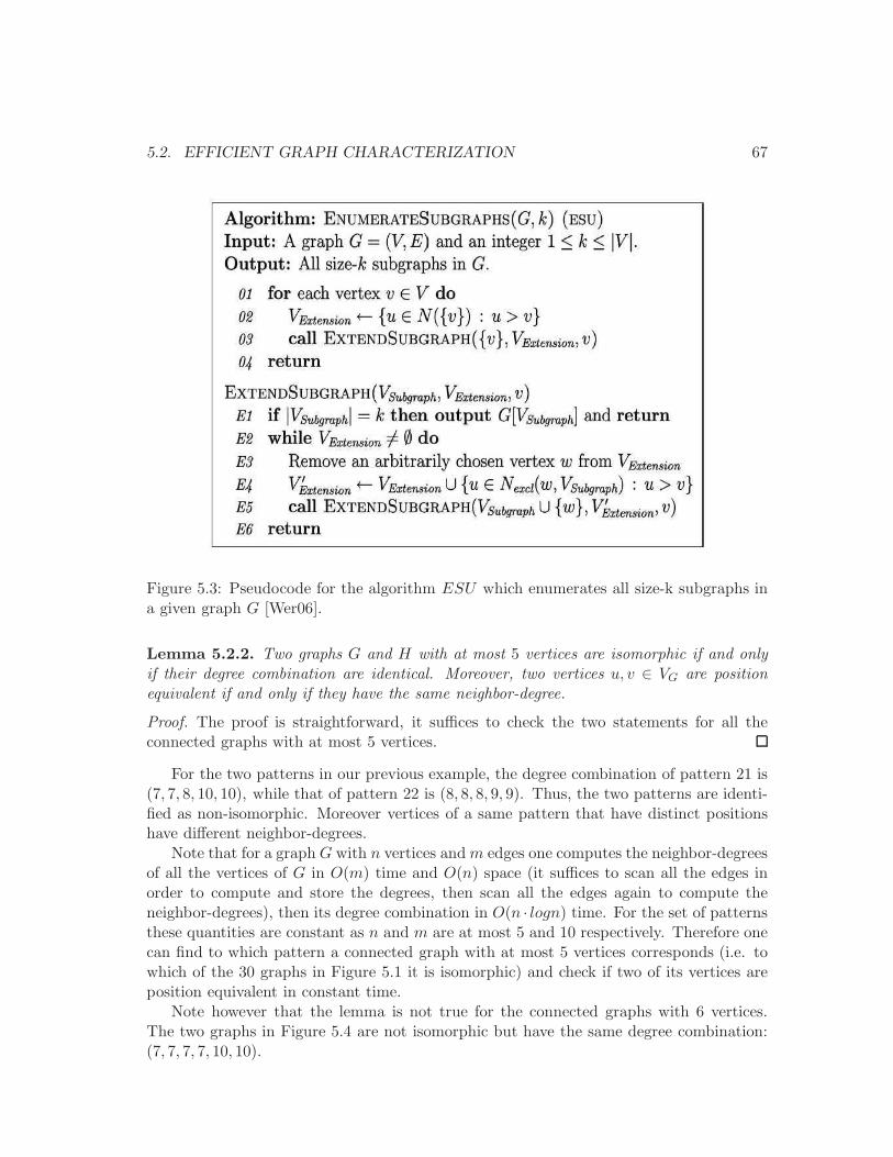
5.2. EFFICIENT GRAPH CHARACTERIZATION 67
Figure 5.3: Pseudocode for the algorithm ESU which enumerates all size-k subgraphs ina given graph G [Wer06].
Lemma 5.2.2. Two graphs G and H with at most 5 vertices are isomorphic if and onlyif their degree combination are identical. Moreover, two vertices u, v ∈ VG are positionequivalent if and only if they have the same neighbor-degree.
Proof. The proof is straightforward, it suffices to check the two statements for all theconnected graphs with at most 5 vertices.
For the two patterns in our previous example, the degree combination of pattern 21 is(7, 7, 8, 10, 10), while that of pattern 22 is (8, 8, 8, 9, 9). Thus, the two patterns are identi-fied as non-isomorphic. Moreover vertices of a same pattern that have distinct positionshave different neighbor-degrees.
Note that for a graph G with n vertices andm edges one computes the neighbor-degreesof all the vertices of G in O(m) time and O(n) space (it suffices to scan all the edges inorder to compute and store the degrees, then scan all the edges again to compute theneighbor-degrees), then its degree combination in O(n · logn) time. For the set of patternsthese quantities are constant as n and m are at most 5 and 10 respectively. Therefore onecan find to which pattern a connected graph with at most 5 vertices corresponds (i.e. towhich of the 30 graphs in Figure 5.1 it is isomorphic) and check if two of its vertices areposition equivalent in constant time.
Note however that the lemma is not true for the connected graphs with 6 vertices.The two graphs in Figure 5.4 are not isomorphic but have the same degree combination:(7, 7, 7, 7, 10, 10).
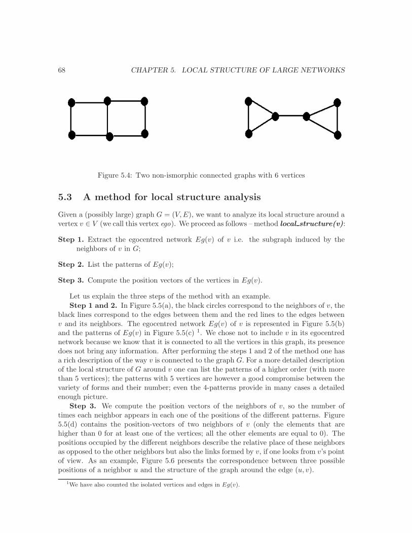
68 CHAPTER 5. LOCAL STRUCTURE OF LARGE NETWORKS
Figure 5.4: Two non-ismorphic connected graphs with 6 vertices
5.3 A method for local structure analysis
Given a (possibly large) graph G = (V,E), we want to analyze its local structure around avertex v ∈ V (we call this vertex ego). We proceed as follows – method local structure(v):
Step 1. Extract the egocentred network Eg(v) of v i.e. the subgraph induced by theneighbors of v in G;
Step 2. List the patterns of Eg(v);
Step 3. Compute the position vectors of the vertices in Eg(v).
Let us explain the three steps of the method with an example.
Step 1 and 2. In Figure 5.5(a), the black circles correspond to the neighbors of v, theblack lines correspond to the edges between them and the red lines to the edges betweenv and its neighbors. The egocentred network Eg(v) of v is represented in Figure 5.5(b)and the patterns of Eg(v) in Figure 5.5(c) 1. We chose not to include v in its egocentrednetwork because we know that it is connected to all the vertices in this graph, its presencedoes not bring any information. After performing the steps 1 and 2 of the method one hasa rich description of the way v is connected to the graph G. For a more detailed descriptionof the local structure of G around v one can list the patterns of a higher order (with morethan 5 vertices); the patterns with 5 vertices are however a good compromise between thevariety of forms and their number; even the 4-patterns provide in many cases a detailedenough picture.
Step 3. We compute the position vectors of the neighbors of v, so the number oftimes each neighbor appears in each one of the positions of the different patterns. Figure5.5(d) contains the position-vectors of two neighbors of v (only the elements that arehigher than 0 for at least one of the vertices; all the other elements are equal to 0). Thepositions occupied by the different neighbors describe the relative place of these neighborsas opposed to the other neighbors but also the links formed by v, if one looks from v’s pointof view. As an example, Figure 5.6 presents the correspondence between three possiblepositions of a neighbor u and the structure of the graph around the edge (u, v).
1We have also counted the isolated vertices and edges in Eg(v).
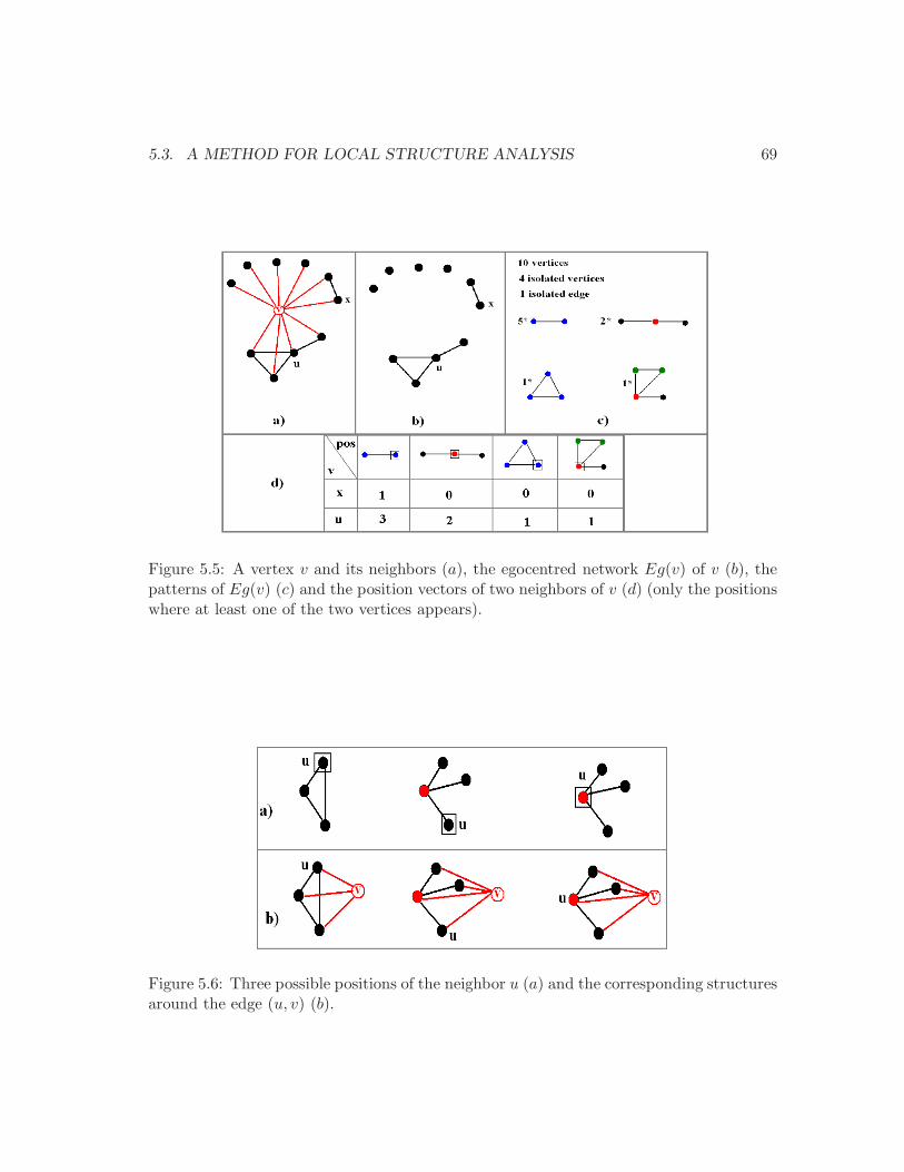
5.3. A METHOD FOR LOCAL STRUCTURE ANALYSIS 69
Figure 5.5: A vertex v and its neighbors (a), the egocentred network Eg(v) of v (b), thepatterns of Eg(v) (c) and the position vectors of two neighbors of v (d) (only the positionswhere at least one of the two vertices appears).
Figure 5.6: Three possible positions of the neighbor u (a) and the corresponding structuresaround the edge (u, v) (b).
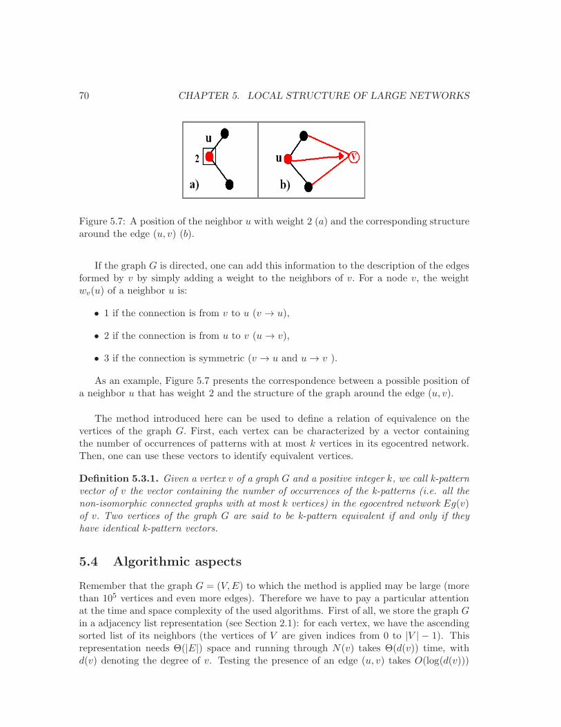
70 CHAPTER 5. LOCAL STRUCTURE OF LARGE NETWORKS
Figure 5.7: A position of the neighbor u with weight 2 (a) and the corresponding structurearound the edge (u, v) (b).
If the graph G is directed, one can add this information to the description of the edgesformed by v by simply adding a weight to the neighbors of v. For a node v, the weightwv(u) of a neighbor u is:
• 1 if the connection is from v to u (v → u),
• 2 if the connection is from u to v (u→ v),
• 3 if the connection is symmetric (v → u and u→ v ).
As an example, Figure 5.7 presents the correspondence between a possible position ofa neighbor u that has weight 2 and the structure of the graph around the edge (u, v).
The method introduced here can be used to define a relation of equivalence on thevertices of the graph G. First, each vertex can be characterized by a vector containingthe number of occurrences of patterns with at most k vertices in its egocentred network.Then, one can use these vectors to identify equivalent vertices.
Definition 5.3.1. Given a vertex v of a graph G and a positive integer k, we call k-patternvector of v the vector containing the number of occurrences of the k-patterns (i.e. all thenon-isomorphic connected graphs with at most k vertices) in the egocentred network Eg(v)of v. Two vertices of the graph G are said to be k-pattern equivalent if and only if theyhave identical k-pattern vectors.
5.4 Algorithmic aspects
Remember that the graph G = (V,E) to which the method is applied may be large (morethan 105 vertices and even more edges). Therefore we have to pay a particular attentionat the time and space complexity of the used algorithms. First of all, we store the graph Gin a adjacency list representation (see Section 2.1): for each vertex, we have the ascendingsorted list of its neighbors (the vertices of V are given indices from 0 to |V | − 1). Thisrepresentation needs Θ(|E|) space and running through N(v) takes Θ(d(v)) time, withd(v) denoting the degree of v. Testing the presence of an edge (u, v) takes O(log(d(v)))
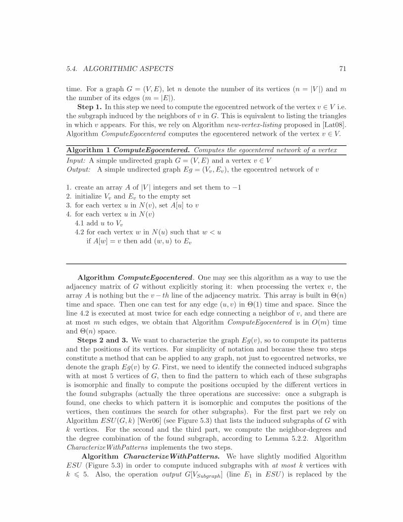
5.4. ALGORITHMIC ASPECTS 71
time. For a graph G = (V,E), let n denote the number of its vertices (n = |V |) and mthe number of its edges (m = |E|).
Step 1. In this step we need to compute the egocentred network of the vertex v ∈ V i.e.the subgraph induced by the neighbors of v in G. This is equivalent to listing the trianglesin which v appears. For this, we rely on Algorithm new-vertex-listing proposed in [Lat08].Algorithm ComputeEgocentered computes the egocentered network of the vertex v ∈ V.
Algorithm 1 ComputeEgocentered. Computes the egocentered network of a vertex
Input: A simple undirected graph G = (V,E) and a vertex v ∈ VOutput: A simple undirected graph Eg = (Vv , Ev), the egocentred network of v
1. create an array A of |V | integers and set them to −12. initialize Vv and Ev to the empty set3. for each vertex u in N(v), set A[u] to v4. for each vertex u in N(v)
4.1 add u to Vv
4.2 for each vertex w in N(u) such that w < uif A[w] = v then add (w, u) to Ev
Algorithm ComputeEgocentered . One may see this algorithm as a way to use theadjacency matrix of G without explicitly storing it: when processing the vertex v, thearray A is nothing but the v− th line of the adjacency matrix. This array is built in Θ(n)time and space. Then one can test for any edge (u, v) in Θ(1) time and space. Since theline 4.2 is executed at most twice for each edge connecting a neighbor of v, and there areat most m such edges, we obtain that Algorithm ComputeEgocentered is in O(m) timeand Θ(n) space.
Steps 2 and 3. We want to characterize the graph Eg(v), so to compute its patternsand the positions of its vertices. For simplicity of notation and because these two stepsconstitute a method that can be applied to any graph, not just to egocentred networks, wedenote the graph Eg(v) by G. First, we need to identify the connected induced subgraphswith at most 5 vertices of G, then to find the pattern to which each of these subgraphsis isomorphic and finally to compute the positions occupied by the different vertices inthe found subgraphs (actually the three operations are successive: once a subgraph isfound, one checks to which pattern it is isomorphic and computes the positions of thevertices, then continues the search for other subgraphs). For the first part we rely onAlgorithm ESU(G, k) [Wer06] (see Figure 5.3) that lists the induced subgraphs of G withk vertices. For the second and the third part, we compute the neighbor-degrees andthe degree combination of the found subgraph, according to Lemma 5.2.2. AlgorithmCharacterizeWithPatterns implements the two steps.
Algorithm CharacterizeWithPatterns. We have slightly modified AlgorithmESU (Figure 5.3) in order to compute induced subgraphs with at most k vertices withk 6 5. Also, the operation output G[VSubgraph] (line E1 in ESU) is replaced by the
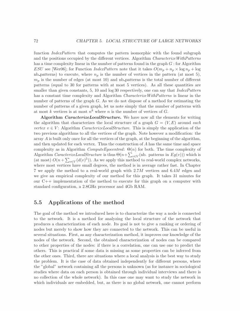
72 CHAPTER 5. LOCAL STRUCTURE OF LARGE NETWORKS
function IndexPattern that computes the pattern isomorphic with the found subgraphand the positions occupied by the different vertices. Algorithm CharacterizeWithPatternshas a time complexity linear in the number of patterns found in the graph G : for AlgorithmESU see [Wer06]; for Function IndexPattern note that it takes O(mp + np × log np + lognb patterns) to execute, where np is the number of vertices in the pattern (at most 5),mp is the number of edges (at most 10) and nb patterns is the total number of differentpatterns (equal to 30 for patterns with at most 5 vertices). As all these quantities aresmaller than given constants, 5, 10 and log 30 respectively, one can say that IndexPatternhas a constant time complexity and Algorithm CharacterizeWithPatterns is linear in thenumber of patterns of the graph G. As we do not dispose of a method for estimating thenumber of patterns of a given graph, let us note simply that the number of patterns withat most k vertices is at most nk where n is the number of vertices of G.
Algorithm CaracterizeLocalStructure. We have now all the elements for writingthe algorithm that characterizes the local structure of a graph G = (V,E) around eachvertex v ∈ V : Algorithm CaracterizeLocalStructure. This is simply the application of thetwo previous algorithms to all the vertices of the graph. Note however a modification: thearray A is built only once for all the vertices of the graph, at the beginning of the algorithm,and then updated for each vertex. Thus the construction of A has the same time and spacecomplexity as in Algorithm ComputeEgocentred : Θ(n) for both. The time complexity ofAlgorithm CaracterizeLocalStructure is thus Θ(n+
∑
v∈V (nb. patterns in Eg(v))) which is(at most) O(n+
∑
v∈V (d(v)5)). As we apply this method to real-world complex networks,
where most vertices have small degrees, the method is in average rather fast. In Chapter7 we apply the method to a real-world graph with 2.7M vertices and 6.4M edges andwe give an empirical complexity of our method for this graph. It takes 31 minutes forour C++ implementation of the method to execute for this graph on a computer withstandard configuration, a 2.8GHz processor and 4Gb RAM.
5.5 Applications of the method
The goal of the method we introduced here is to characterize the way a node is connectedto the network. It is a method for analyzing the local structure of the network thatproduces a characterization of each node. Its goal is not to give a ranking or ordering ofnodes but merely to show how they are connected to the network. This can be useful inseveral situations. First, as any characterization method, it improves our knowledge of thenodes of the network. Second, the obtained characterization of nodes can be comparedto other properties of the nodes: if there is a correlation, one can use one to predict theothers. This is practical if some data is missing as some properties can be inferred fromthe other ones. Third, there are situations where a local analysis is the best way to studythe problem. It is the case of data obtained independently for different persons, wherethe ”global” network containing all the persons is unknown (as for instance in sociologicalstudies where data on each person is obtained through individual interviews and there isno collection of the whole network). In this case one may want to study the network inwhich individuals are embedded, but, as there is no global network, one cannot perform

5.5. APPLICATIONS OF THE METHOD 73
Algorithm 2 CharacterizeWithPatterns. Characterizes an undirected simple graph
Input: A simple undirected graph G = (V,E) and a positive integer k 6 5Output: An array Pt such that Pt[P ] contains the nb. of occurrences of the pattern P in G,an array Ps such that Ps[v][i] = Posk(G, v, i) (the nb. of occurrences of v in the position i)
1. set all the elements of Pt and Ps to 02. for each vertex v ∈ V do
2.1 Vextension ←− {u ∈ N(v) : u > v}2.2 VSubgraph = {v}, ESubgraph = ∅2.3 call ExtendSubgraph(VSubgraph, ESubgraph, VExtension, v, P t, Ps, k)
3. return
ExtendSubgraphInput:- a positive integer k 6 5,- two sets VSubgraph ⊆ V and ESubgraph ⊆ E containing the vertices and edgesalready added to the subgraph,
- a set of vertices Vextension containing the vertices that can be added to the subgraph,- a vertex v from which the construction of the subgraph has begun,- two arrays Pt and Ps that will be updated by the procedure
1. if |VSubgraph| > k return2. if |VSubgraph| > 0 call IndexPattern(VSubgraph, ESubgraph,Pt, Ps )3. while VExtension 6= ∅
3.1. remove an arbitrarily chosen vertex w from VExtension
3.2. V ′Extension = VExtension
3.3. E′Subgraph = ESubgraph
3.4. for each u ∈ N(w) : u > vif u ∈ VSubgraph add (u,w) to E′
Subgraph //add all the edges from w to the subgraph
else if u /∈ N(VSubgraph) add u to V ′Extension
3.5. call ExtendSubgraph(VSubgraph ∪ {w} , E′Subgraph, V
′Extension, v, P t, Ps, k )
IndexPatternInput: A set of vertices VSubgraph, a set of edges ESubgraph andtwo arrays Pt and Ps that will be updated by the procedure
1. scan the set ESubgraph and note each occurrence of each vertex//thus computing the degrees of the vertices
2. create an array D containing the degrees of the vertices3. for each edge (a, b) ∈ ESubgraph add degree(b) to D(a) and degree(a) to D(b)
//thus computing the neighbor-degrees4. sort D and write it as a number5. find the pattern P with this number and increment Pt(P )6. for each vertex u
find the position i (in the pattern P ) with the same neighbor-degree and increment Ps[u][i]
74 CHAPTER 5. LOCAL STRUCTURE OF LARGE NETWORKS
Algorithm 3 CaracterizeLocalStructure Characterizes the local structure around eachvertex in a (large) graph
Input: A simple undirected graph G = (V,E) and a positive integer k 6 5
1. create an array A of |V | integers and set them to −12. for each vertex v ∈ V
2.1 initialize Vv and Ev to the empty set2.2 for each vertex u in N(v), set A[u] to v2.3 for each vertex u in N(v)
2.3.1 add u to Vv
2.3.2 for each vertex w in N(u) such that w < uif A[w] = v then add (w, u) to Ev
2.4 call CharacterizeWithPatterns((Vv , Ev), k)
the classical global or intermediate network analysis.
Another situation where the study of the local structure is appropriate is for networkswhere nodes ”importance” is local. In the opposite situation, there are networks where(some) nodes are important for the function of the whole network. Take for instance thecase of the railways network of a country; in this case it is important to analyze nodesin the context of the global network: there are some nodes (railways stations) that areimportant for the whole network as they connect different parts of the country. In this casea local analysis is not sufficient, one needs to use measures that take into considerationthe whole network. Also, in online social networks, the global perspective may be useful.In this case users are visible to the whole network: they can be seen and contacted byany other user in the network. Often there is a notion of popularity, where people tryto improve their visibility and where fans can link to them. However, a local analysismay also bring important information. One can analyze for instance the links created bydifferent persons before a certain moment in time; this is a local analysis that outputsstar-fan relations (expressed by links).
A local approach is useful especially in networks where nodes importance and visibilityare local. Take for instance the case of mobile phone communications. Here people cannotbe contacted by everybody as mobile phone numbers are not public. And even if that wasthe case, people do not usually call other people just because these are known or famous.There is no measure of popularity in this network (as opposed to online platforms wheredifferent statistics on people activity and popularity are often available). People usuallymake phone calls because they really have something to discuss with the other person andnot because they are fans of this person. In this case people a few steps away (maybe2 suffice) from a person do not know this person; the existence of this person does nothave any importance to them. For such networks characterizing nodes by looking at thewhole network may not be very useful: someone with a high (say betweenness) centralitymay not be more important than other persons. His presence in the network is surelyimportant for several persons but these persons are most probably close to him in the

5.6. COMPARISON TO OTHER MEASURES 75
Table 5.1: Equivalent notions for a vertex v: in the whole graph and in the egocentrednetwork.
graph G egocentred network Eg(v)
degree of v number of vertices
number of triangles containing v number of edges
number of 4-cliques containing v number of triangles
network. If this person leaves the network the vast majority of the other individuals in thenetwork won’t even notice the change. For such networks the method introduced here ismore appropriate that other types of analysis taking into consideration the whole network(at least when characterizing each node).
Finally, this method can be used in order to compute a certain equivalence or similarityof vertices, notions very important for the definition of social roles played by nodes in anetwork. A possible relation of equivalence is the k-pattern equivalence that we havedefined in Section 5.3. If one wants to compute similar vertices (instead of equivalent),one can compute a certain distance between the k-pattern vectors of the vertices (alsodefined in Section 5.3). We will discuss this approach and some applications in Chapter8.
5.6 Comparison to other measures
Let us first emphasize the equivalence between several notions regarding a vertex v, in thecontext of the whole graph and in its egocentred network (see Table 5.1). For instance,the degree of v in the graph G corresponds to the number of vertices in the egocentredgraph Eg(v). Moreover the clustering coefficient of the node v is equal to the densityof its egocentred network, as the number of triangles containing the node is equal to thenumber of edges between its neighbors, and are both equal to
(
d2
)
where d is the degree of v.
Patterns versus centrality. As presented in Section 3.1, the centrality of verticesis a measure of their importance in the network. Usually one computes the centrality ofall the vertices in the graph in order to produce a ranking of vertices. There are severaldefinitions of centrality: the degree centrality, the betweenness, the closeness, the page-rank, the eigen vector centrality etc. Besides the degree centrality (which is simply thedegree of the node), all the other measures take into consideration the entire graph. Asexplained in the previous section, the goal of the method introduced here is to produce alocal characterization of vertices. This is the main difference between our method and thedifferent definitions of centrality: the goal is not the same. Another difference comes fromthe context of application of the methods: while the different measures of centrality needto have the entire network in order to compute the centrality of one node, our methodneeds only the neighbors of the node and the edges between them, so it can be applied onlyto some parts of the graph if the other parts are not known. Finally, the betweenness andcloseness centrality can be hardly computed in complex networks as their time complexity
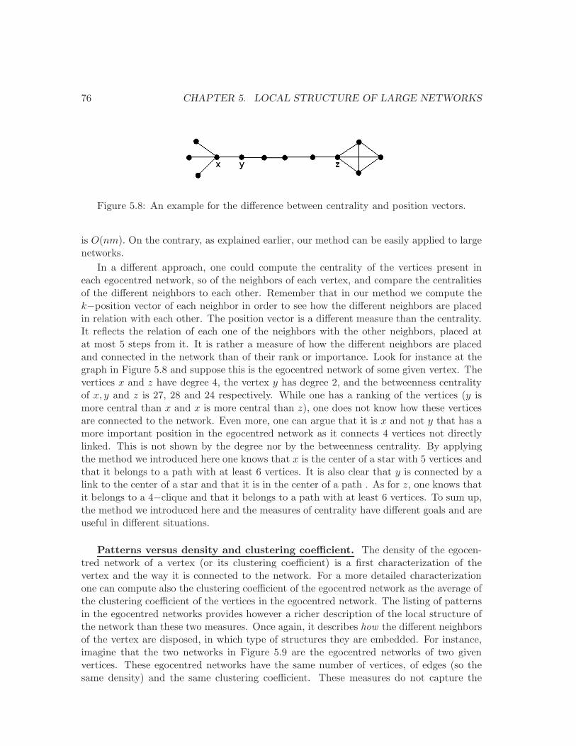
76 CHAPTER 5. LOCAL STRUCTURE OF LARGE NETWORKS
Figure 5.8: An example for the difference between centrality and position vectors.
is O(nm). On the contrary, as explained earlier, our method can be easily applied to largenetworks.
In a different approach, one could compute the centrality of the vertices present ineach egocentred network, so of the neighbors of each vertex, and compare the centralitiesof the different neighbors to each other. Remember that in our method we compute thek−position vector of each neighbor in order to see how the different neighbors are placedin relation with each other. The position vector is a different measure than the centrality.It reflects the relation of each one of the neighbors with the other neighbors, placed atat most 5 steps from it. It is rather a measure of how the different neighbors are placedand connected in the network than of their rank or importance. Look for instance at thegraph in Figure 5.8 and suppose this is the egocentred network of some given vertex. Thevertices x and z have degree 4, the vertex y has degree 2, and the betweenness centralityof x, y and z is 27, 28 and 24 respectively. While one has a ranking of the vertices (y ismore central than x and x is more central than z), one does not know how these verticesare connected to the network. Even more, one can argue that it is x and not y that has amore important position in the egocentred network as it connects 4 vertices not directlylinked. This is not shown by the degree nor by the betweenness centrality. By applyingthe method we introduced here one knows that x is the center of a star with 5 vertices andthat it belongs to a path with at least 6 vertices. It is also clear that y is connected by alink to the center of a star and that it is in the center of a path . As for z, one knows thatit belongs to a 4−clique and that it belongs to a path with at least 6 vertices. To sum up,the method we introduced here and the measures of centrality have different goals and areuseful in different situations.
Patterns versus density and clustering coefficient. The density of the egocen-tred network of a vertex (or its clustering coefficient) is a first characterization of thevertex and the way it is connected to the network. For a more detailed characterizationone can compute also the clustering coefficient of the egocentred network as the average ofthe clustering coefficient of the vertices in the egocentred network. The listing of patternsin the egocentred networks provides however a richer description of the local structure ofthe network than these two measures. Once again, it describes how the different neighborsof the vertex are disposed, in which type of structures they are embedded. For instance,imagine that the two networks in Figure 5.9 are the egocentred networks of two givenvertices. These egocentred networks have the same number of vertices, of edges (so thesame density) and the same clustering coefficient. These measures do not capture the
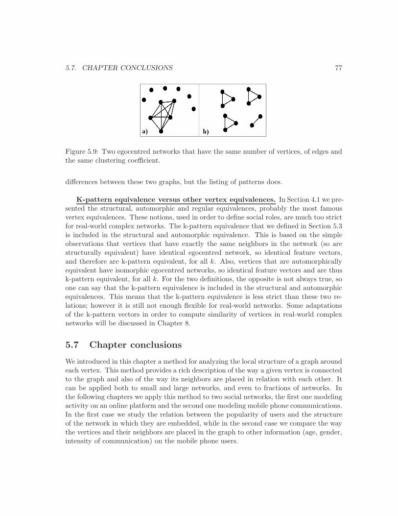
5.7. CHAPTER CONCLUSIONS 77
Figure 5.9: Two egocentred networks that have the same number of vertices, of edges andthe same clustering coefficient.
differences between these two graphs, but the listing of patterns does.
K-pattern equivalence versus other vertex equivalences. In Section 4.1 we pre-sented the structural, automorphic and regular equivalences, probably the most famousvertex equivalences. These notions, used in order to define social roles, are much too strictfor real-world complex networks. The k-pattern equivalence that we defined in Section 5.3is included in the structural and automorphic equivalence. This is based on the simpleobservations that vertices that have exactly the same neighbors in the network (so arestructurally equivalent) have identical egocentred network, so identical feature vectors,and therefore are k-pattern equivalent, for all k. Also, vertices that are automorphicallyequivalent have isomorphic egocentred networks, so identical feature vectors and are thusk-pattern equivalent, for all k. For the two definitions, the opposite is not always true, soone can say that the k-pattern equivalence is included in the structural and automorphicequivalences. This means that the k-pattern equivalence is less strict than these two re-lations; however it is still not enough flexible for real-world networks. Some adaptationsof the k-pattern vectors in order to compute similarity of vertices in real-world complexnetworks will be discussed in Chapter 8.
5.7 Chapter conclusions
We introduced in this chapter a method for analyzing the local structure of a graph aroundeach vertex. This method provides a rich description of the way a given vertex is connectedto the graph and also of the way its neighbors are placed in relation with each other. Itcan be applied both to small and large networks, and even to fractions of networks. Inthe following chapters we apply this method to two social networks, the first one modelingactivity on an online platform and the second one modeling mobile phone communications.In the first case we study the relation between the popularity of users and the structureof the network in which they are embedded, while in the second case we compare the waythe vertices and their neighbors are placed in the graph to other information (age, gender,intensity of communication) on the mobile phone users.

78 CHAPTER 5. LOCAL STRUCTURE OF LARGE NETWORKS
Chapter 6
From online popularity to sociallinkage: a case study of MySpace
6.1 Introduction
In this chapter we analyze the popularity of users’ content on MySpace in relation withthe social network in which the users are embedded. MySpace (www.myspace.com) isan online platform for social networking which gives signed-up users a free access to apersonal space. In this space, users can present information about themselves, create ablog, publish different content, link to other users, visit their pages and write commentsthere. Although users can publish any kind of photos or videos, MySpace is especiallyknown for the great number of music artists who present their musical compositions. Eachuser can declare his profile type as ”member” or ”musician”. Besides being a place forpublishing content, MySpace also offer its users the possibility to connect to each other.Thus, everybody can visit everybody’s page and write comments there. Also each user canlink to any other user by declaring friendship or best-friendship relations. These relationsare not necessarily mutual: everybody can declare everybody as (best) friend, withoutwaiting for the acceptance of the other part. The number of best friendship declarationsis limited to 40, so one can consider the best friend links as stronger than the friend ones.
On the page of each user, all this information is visible: besides the published contentand personal data, everybody sees how many people visited or left comments on theprofile, how many users have declared him as (best) friend and how many users he hasdeclared. Each user, thanks to these ratings on how many people viewed or commented hiswork, knows how popular his profile is. He can thus adjust his publishing and networkingpractices in order to become more popular, so he can develop strategies to increase hisfame. Every user is manager of his own visibility thus transforming MySpace in a placefor competition for popularity. The same situation happens on other online platforms thatoffer social networking tools and space for content publishing.
Several researchers have dealt with this competition for visibility and reputation ononline platforms. Some of them concentrated on the success of contents while othersfocused on the reputation of individuals in the large social networks created by these
79
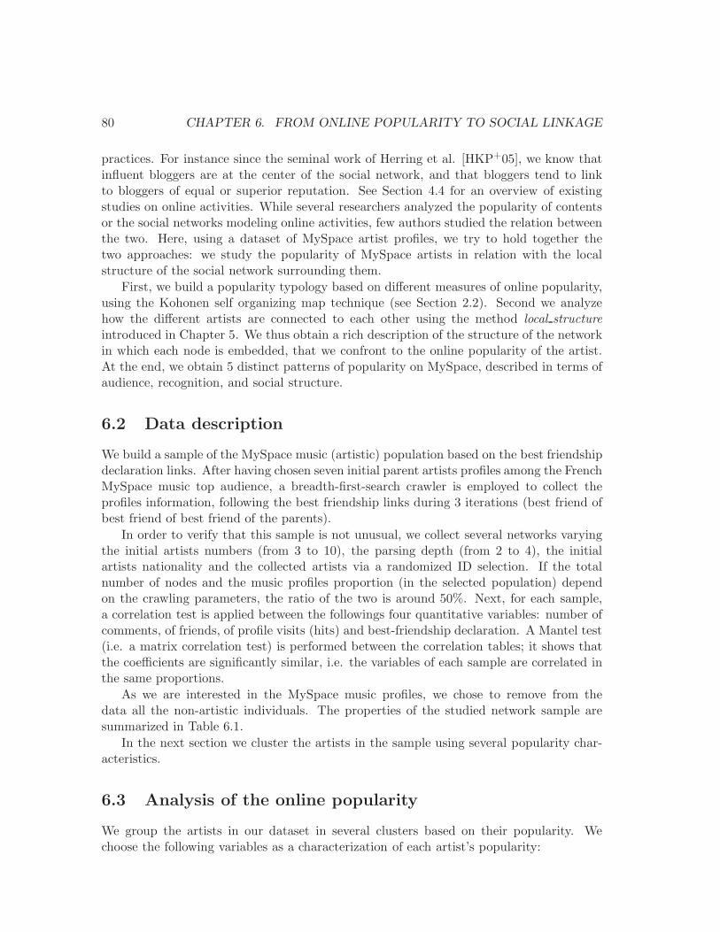
80 CHAPTER 6. FROM ONLINE POPULARITY TO SOCIAL LINKAGE
practices. For instance since the seminal work of Herring et al. [HKP+05], we know thatinfluent bloggers are at the center of the social network, and that bloggers tend to linkto bloggers of equal or superior reputation. See Section 4.4 for an overview of existingstudies on online activities. While several researchers analyzed the popularity of contentsor the social networks modeling online activities, few authors studied the relation betweenthe two. Here, using a dataset of MySpace artist profiles, we try to hold together thetwo approaches: we study the popularity of MySpace artists in relation with the localstructure of the social network surrounding them.
First, we build a popularity typology based on different measures of online popularity,using the Kohonen self organizing map technique (see Section 2.2). Second we analyzehow the different artists are connected to each other using the method local structureintroduced in Chapter 5. We thus obtain a rich description of the structure of the networkin which each node is embedded, that we confront to the online popularity of the artist.At the end, we obtain 5 distinct patterns of popularity on MySpace, described in terms ofaudience, recognition, and social structure.
6.2 Data description
We build a sample of the MySpace music (artistic) population based on the best friendshipdeclaration links. After having chosen seven initial parent artists profiles among the FrenchMySpace music top audience, a breadth-first-search crawler is employed to collect theprofiles information, following the best friendship links during 3 iterations (best friend ofbest friend of best friend of the parents).
In order to verify that this sample is not unusual, we collect several networks varyingthe initial artists numbers (from 3 to 10), the parsing depth (from 2 to 4), the initialartists nationality and the collected artists via a randomized ID selection. If the totalnumber of nodes and the music profiles proportion (in the selected population) dependon the crawling parameters, the ratio of the two is around 50%. Next, for each sample,a correlation test is applied between the followings four quantitative variables: number ofcomments, of friends, of profile visits (hits) and best-friendship declaration. A Mantel test(i.e. a matrix correlation test) is performed between the correlation tables; it shows thatthe coefficients are significantly similar, i.e. the variables of each sample are correlated inthe same proportions.
As we are interested in the MySpace music profiles, we chose to remove from thedata all the non-artistic individuals. The properties of the studied network sample aresummarized in Table 6.1.
In the next section we cluster the artists in the sample using several popularity char-acteristics.
6.3 Analysis of the online popularity
We group the artists in our dataset in several clusters based on their popularity. Wechoose the following variables as a characterization of each artist’s popularity:
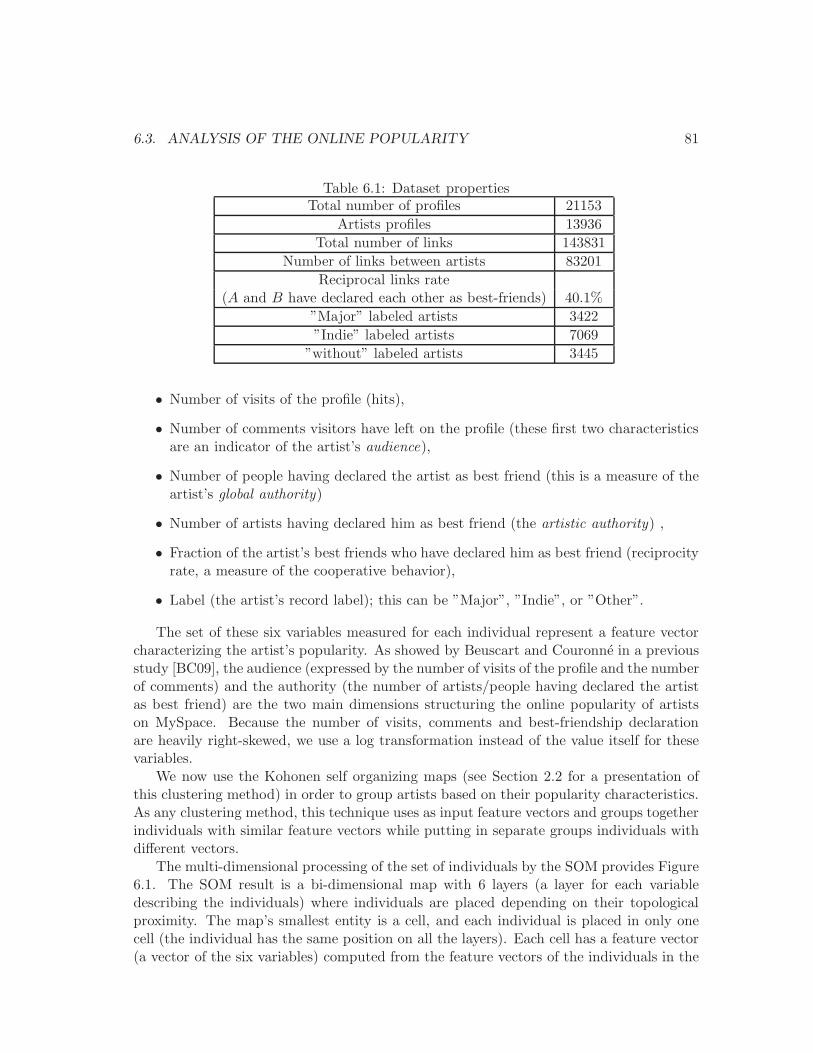
6.3. ANALYSIS OF THE ONLINE POPULARITY 81
Table 6.1: Dataset propertiesTotal number of profiles 21153
Artists profiles 13936
Total number of links 143831
Number of links between artists 83201
Reciprocal links rate(A and B have declared each other as best-friends) 40.1%
”Major” labeled artists 3422
”Indie” labeled artists 7069
”without” labeled artists 3445
• Number of visits of the profile (hits),
• Number of comments visitors have left on the profile (these first two characteristicsare an indicator of the artist’s audience),
• Number of people having declared the artist as best friend (this is a measure of theartist’s global authority)
• Number of artists having declared him as best friend (the artistic authority) ,
• Fraction of the artist’s best friends who have declared him as best friend (reciprocityrate, a measure of the cooperative behavior),
• Label (the artist’s record label); this can be ”Major”, ”Indie”, or ”Other”.
The set of these six variables measured for each individual represent a feature vectorcharacterizing the artist’s popularity. As showed by Beuscart and Couronne in a previousstudy [BC09], the audience (expressed by the number of visits of the profile and the numberof comments) and the authority (the number of artists/people having declared the artistas best friend) are the two main dimensions structuring the online popularity of artistson MySpace. Because the number of visits, comments and best-friendship declarationare heavily right-skewed, we use a log transformation instead of the value itself for thesevariables.
We now use the Kohonen self organizing maps (see Section 2.2 for a presentation ofthis clustering method) in order to group artists based on their popularity characteristics.As any clustering method, this technique uses as input feature vectors and groups togetherindividuals with similar feature vectors while putting in separate groups individuals withdifferent vectors.
The multi-dimensional processing of the set of individuals by the SOM provides Figure6.1. The SOM result is a bi-dimensional map with 6 layers (a layer for each variabledescribing the individuals) where individuals are placed depending on their topologicalproximity. The map’s smallest entity is a cell, and each individual is placed in only onecell (the individual has the same position on all the layers). Each cell has a feature vector(a vector of the six variables) computed from the feature vectors of the individuals in the
82 CHAPTER 6. FROM ONLINE POPULARITY TO SOCIAL LINKAGE
Figure 6.1: Self Organizing map of the artists depending on their popularity properties.
cell. On each layer, the color of the cell corresponds to the value of the correspondingvariable for that cell. The interest of this method of clustering is the visual representationof the population for each one the variables. Instead of the classical representation ofindividuals into clusters, where one does not know how the different variables contributeto individual proximity, this method provides a representation of both proximity betweenindividuals and values of variables for the different individuals.
The obtained map appears to be structured by two independent trends: the more anartist belongs to a southern cell, the more his popularity is high, in terms of both audienceand authority; and the more an artist is to the west side, the more he tends to havereciprocal links. If audience and authority are partly correlated and discriminate popularartists from anonymous, the trends are not exactly similar. Indeed, the south-westernarea is associated with the authoritative elites (highest artistic and global authority) andthe south-eastern area is associated with the most notorious artists (highest page viewsand comments). If, most probably, the audience elites are not without authority andauthoritative elites are not without audience, the top artists of the audience and of theauthority do not overlap.
We can note that the two measures of authority (global and artistic) are correlated.The artists and the other fans create in the same way their best friendship links: theauthority hierarchy follows a unique trend. Complementary, this result shows that thereciprocal links behavior is not associated with the popularity: it may be either becausean authoritative artist cannot have more than 40 best friends (and therefore cannot citeeverybody) or because very authoritative artists are not linking back to people who link tothem (fan-star relationship). Finally we observe that the south-east area (audience elites)is associated with a strong presence of the ”Major” labels.
We cluster the cells produced by the SOM using a k−means clustering. The expecta-tion maximization algorithm is then employed to choose the best number of clusters. Thepopulation is thus distributed into 5 clusters (Figure 6.2):
6.3. ANALYSIS OF THE ONLINE POPULARITY 83
Figure 6.2: The 5 clusters
Cluster1 (Cyan, population: 2732) gathers artists with a medium-to-large audience, alow authority and a weak reciprocity rate. They are mostly associated with majormusic labels. Our browsing of the Myspace pages of some artists in this clustersuggests that these artists, already popular offline, use their MySpace page as adisplay window of their music, but make very little use of the social networking tools.We may suppose that their strong audience comes from their offline popularity, butthat they are not active enough to gain a strong influence on MySpace.
Cluster2 (Dark blue, pop.: 3036) gathers artists with a very strong authority, and amedium-to-high audience: these artists are not the most popular, but they are themost recommended. Most of them belong to independent labels. The qualitativebrowsing of their pages suggests a very intensive use of the social networking toolsin order to build their online popularity. Here we find a lot of trendy groups andelectronic avant-garde music, waiting for their online fame to become larger.
Cluster3 (Green, pop.: 1920) gathers artists with both a large audience and a strong au-thority, the MySpace elites. They have mostly major labels. Browsing their pages,we find established artists, combining traditional forms of artistic accomplishment(famous labels, presence in renowned festivals) with an active online marketing strat-egy.
Cluster4 (Brown, pop.: 2834) gathers artists with a very small audience and no authority.Most of their pages display very low activity, suggesting that these artists have eitherabandoned the page or show very little interest in online socializing practices.
Cluster5 (Orange, pop.: 2834) gathers artists with a small audience, low authority, and astrong reciprocity rate. Most of them are unsigned. On the contrary to artists fromcluster 4, most of the pages we browsed are very active. These small amateur artistsseem to be the ones populating the local music scenes; they are well connected toother artists from the same scene or from the same geographical area. Their smallaudience may not reflect their inability to reach an audience, but the small size oftheir musical or geographical niche.
This first part of the study provides a classification of artists based on the popularityvariables. The main results are that the two dimensions of the popularity (audience and
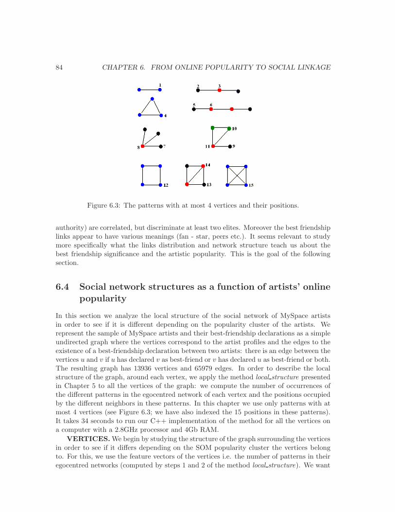
84 CHAPTER 6. FROM ONLINE POPULARITY TO SOCIAL LINKAGE
Figure 6.3: The patterns with at most 4 vertices and their positions.
authority) are correlated, but discriminate at least two elites. Moreover the best friendshiplinks appear to have various meanings (fan - star, peers etc.). It seems relevant to studymore specifically what the links distribution and network structure teach us about thebest friendship significance and the artistic popularity. This is the goal of the followingsection.
6.4 Social network structures as a function of artists’ online
popularity
In this section we analyze the local structure of the social network of MySpace artistsin order to see if it is different depending on the popularity cluster of the artists. Werepresent the sample of MySpace artists and their best-friendship declarations as a simpleundirected graph where the vertices correspond to the artist profiles and the edges to theexistence of a best-friendship declaration between two artists: there is an edge between thevertices u and v if u has declared v as best-friend or v has declared u as best-friend or both.The resulting graph has 13936 vertices and 65979 edges. In order to describe the localstructure of the graph, around each vertex, we apply the method local structure presentedin Chapter 5 to all the vertices of the graph: we compute the number of occurrences ofthe different patterns in the egocentred network of each vertex and the positions occupiedby the different neighbors in these patterns. In this chapter we use only patterns with atmost 4 vertices (see Figure 6.3; we have also indexed the 15 positions in these patterns).It takes 34 seconds to run our C++ implementation of the method for all the vertices ona computer with a 2.8GHz processor and 4Gb RAM.
VERTICES.We begin by studying the structure of the graph surrounding the verticesin order to see if it differs depending on the SOM popularity cluster the vertices belongto. For this, we use the feature vectors of the vertices i.e. the number of patterns in theiregocentred networks (computed by steps 1 and 2 of the method local structure). We want
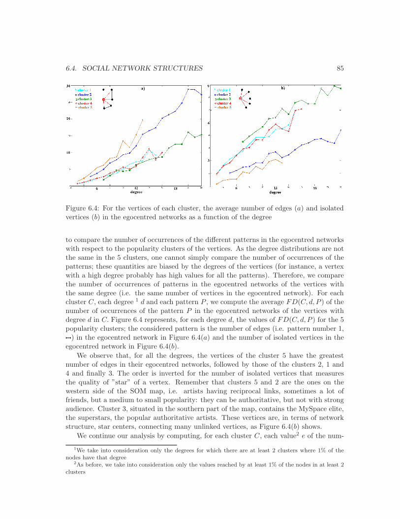
6.4. SOCIAL NETWORK STRUCTURES 85
Figure 6.4: For the vertices of each cluster, the average number of edges (a) and isolatedvertices (b) in the egocentred networks as a function of the degree
to compare the number of occurrences of the different patterns in the egocentred networkswith respect to the popularity clusters of the vertices. As the degree distributions are notthe same in the 5 clusters, one cannot simply compare the number of occurrences of thepatterns; these quantities are biased by the degrees of the vertices (for instance, a vertexwith a high degree probably has high values for all the patterns). Therefore, we comparethe number of occurrences of patterns in the egocentred networks of the vertices withthe same degree (i.e. the same number of vertices in the egocentred network). For eachcluster C, each degree 1 d and each pattern P , we compute the average FD(C, d, P ) of thenumber of occurrences of the pattern P in the egocentred networks of the vertices withdegree d in C. Figure 6.4 represents, for each degree d, the values of FD(C, d, P ) for the 5popularity clusters; the considered pattern is the number of edges (i.e. pattern number 1,) in the egocentred network in Figure 6.4(a) and the number of isolated vertices in the
egocentred network in Figure 6.4(b).
We observe that, for all the degrees, the vertices of the cluster 5 have the greatestnumber of edges in their egocentred networks, followed by those of the clusters 2, 1 and4 and finally 3. The order is inverted for the number of isolated vertices that measuresthe quality of ”star” of a vertex. Remember that clusters 5 and 2 are the ones on thewestern side of the SOM map, i.e. artists having reciprocal links, sometimes a lot offriends, but a medium to small popularity: they can be authoritative, but not with strongaudience. Cluster 3, situated in the southern part of the map, contains the MySpace elite,the superstars, the popular authoritative artists. These vertices are, in terms of networkstructure, star centers, connecting many unlinked vertices, as Figure 6.4(b) shows.
We continue our analysis by computing, for each cluster C, each value2 e of the num-
1We take into consideration only the degrees for which there are at least 2 clusters where 1% of thenodes have that degree
2As before, we take into consideration only the values reached by at least 1% of the nodes in at least 2clusters
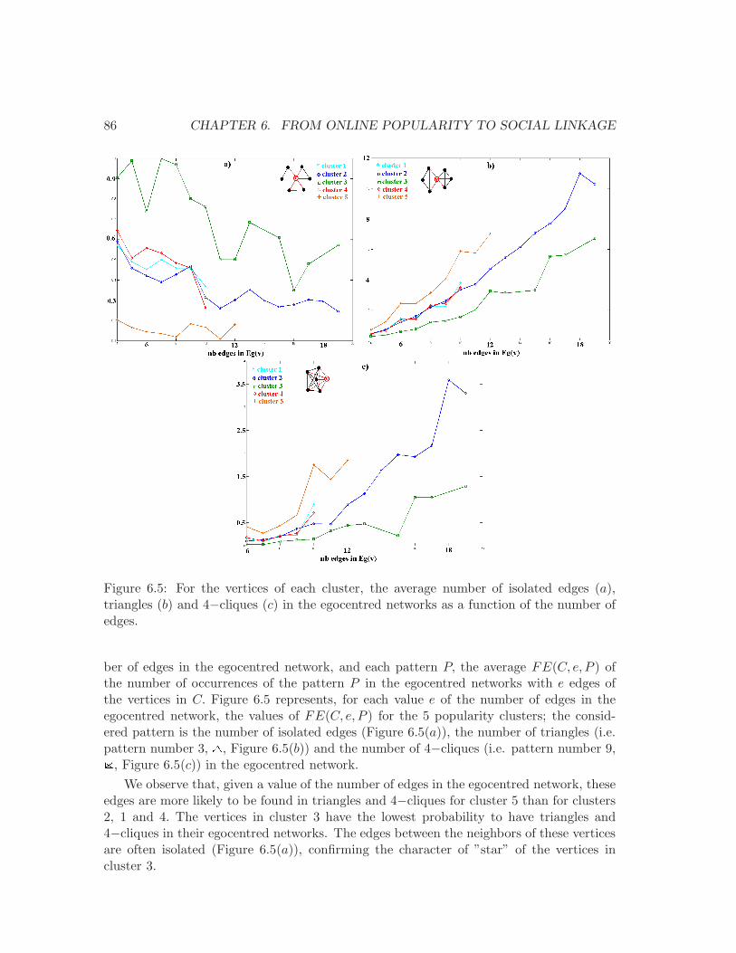
86 CHAPTER 6. FROM ONLINE POPULARITY TO SOCIAL LINKAGE
Figure 6.5: For the vertices of each cluster, the average number of isolated edges (a),triangles (b) and 4−cliques (c) in the egocentred networks as a function of the number ofedges.
ber of edges in the egocentred network, and each pattern P, the average FE(C, e, P ) ofthe number of occurrences of the pattern P in the egocentred networks with e edges ofthe vertices in C. Figure 6.5 represents, for each value e of the number of edges in theegocentred network, the values of FE(C, e, P ) for the 5 popularity clusters; the consid-ered pattern is the number of isolated edges (Figure 6.5(a)), the number of triangles (i.e.pattern number 3, , Figure 6.5(b)) and the number of 4−cliques (i.e. pattern number 9,, Figure 6.5(c)) in the egocentred network.
We observe that, given a value of the number of edges in the egocentred network, theseedges are more likely to be found in triangles and 4−cliques for cluster 5 than for clusters2, 1 and 4. The vertices in cluster 3 have the lowest probability to have triangles and4−cliques in their egocentred networks. The edges between the neighbors of these verticesare often isolated (Figure 6.5(a)), confirming the character of ”star” of the vertices incluster 3.
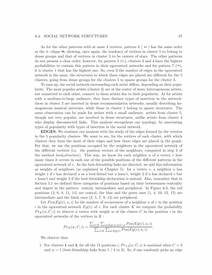
6.4. SOCIAL NETWORK STRUCTURES 87
As for the other patterns with at most 4 vertices, pattern 8 ( ) has the same orderas the 4−clique , showing, once again, the tendency of vertices in cluster 5 to belong todense groups and that of vertices in cluster 3 to be centers of stars. The other patternsdo not present a clear order; however, for pattern 5 ( ), clusters 3 and 4 have the highestprobabilities to contain this pattern in their egocentred networks and for pattern 7 ( ),it is cluster 1 that has the highest one. So, even if the number of edges in the egocentrednetwork is the same, the structures in which these edges are placed are different for the 5clusters, going from dense groups for the clusters 5 to sparse groups for the cluster 3.
To sum up, the social network surrounding each artist differs, depending on their popu-larity. The most popular artists (cluster 3) are at the center of stars; heterogeneous artists,not connected to each other, connect to these artists due to their popularity. As for artistswith a medium-to-large audience, they have distinct types of insertion in the network:those in cluster 2 are inserted in dense recommendation networks, usually describing ho-mogeneous musical universes, while those in cluster 1 belong to sparse structures. Thesame observation can be made for artists with a small audience: artists from cluster 5,though not very popular, are involved in dense structures, unlike artists from cluster 4who display disconnected links. This analysis strengthens our typology, by associatingtypes of popularity with types of insertion in the social network.
EDGES. We continue our analysis with the study of the edges formed by the verticesin the 5 popularity clusters. We want to see, for the vertices of each cluster, with whichclusters they form the most of their edges and how these edges are placed in the graph.For that, we use the positions occupied by the neighbors in the egocentred network ofthe different vertices (i.e. the position vectors of the neighbors, computed in step 3 ofthe method local structure). This way, we know for each neighbor u of a vertex v howmany times it occurs in each one of the possible positions of the different patterns in theegocentred network of v. As the best-friendship links are directed, we add this informationas weights of neighbors (as explained in Chapter 5): for a vertex v, a neighbor u hasweight 1 if v has declared u as a best-friend but u hasn’t, weight 2 if u has declared v butv hasn’t and weight 3 if the best-friendship declaration is mutual. Also, remember that inSection 5.1 we defined three categories of positions based on their betweenness centralityand degree in the pattern: central, intermediate and peripheral. In Figure 6.3, the redpositions (3, 6, 8, 11, 14) are central, the blue and the green ones (1, 4, 10, 12, 15) areintermediate and the black ones (2, 5, 7, 9, 13) are peripheral.
Let Pos(Eg(v), u, i) be the number of occurrences of a neighbor u of v in the positioni in the egocentred network Eg(v) of v. For each cluster K we compute the probabilityPrK(w,C, i) to observe a vertex with weight w of the cluster C in the position i in theegocentred networks of the vertices in K :
PrK(w,C, i) =
∑
v∈K
∑
u∈Eg(v),u∈C,w Pos(Eg(v), u, i)∑
v∈K
∑
u∈Eg(v) Pos(Eg(v), u, i).
We observe that:
1. For clusters 1 and 4, for all the 15 positions i, Pr1,4(w,C, i) is maximal when C = 3and w = 1 (best-friendship links from 1 / 4 to 3). So, if one randomly picks an edge
88 CHAPTER 6. FROM ONLINE POPULARITY TO SOCIAL LINKAGE
formed by a vertex of the cluster 1 or 4, no matter the structure of the graph inwhich this edge is embedded, it is very probable that this edge is an out-going arcto the cluster 3. It is a star-fan relation that confirms the character of ”star” of thevertices in the cluster 3 and the weak authority of the clusters 1 and 4.
2. For cluster 2, for all the positions i, Pr2(w,C, i) is maximal when C = 2 and w = 3(mutual best-friendship links inside the cluster). So the cluster 2, grouping artistswith high (but smaller than the stars’) authority and audience connects mostly toitself.
3. For cluster 3, for all the central and intermediate positions, Pr3(w,C, i) is maximalwhen C = 3 and w = 3; for all the peripheral positions i.e. i ∈ {2, 5, 7, 9, 13},Pr3(w,C, i) is maximal when C = 4 and w = 2 (best-friendship links from 4 to 3).So the edges formed by the vertices of cluster 3 are placed in ”important” positionswhen they are formed inside the cluster and in peripheral positions when they arein-coming arcs. The important positions (as, for instance, position 7, the center of astar) signify that the vertices of the cluster 3 often form a central axis to which manytriangles are connected i.e. many vertices, not connected to each other, connect totwo linked vertices of the cluster 3. This may correspond to two popular artists of asimilar music genre, where people who like the first are highly probable to like thesecond too.
4. For cluster 5, for all the positions with a high degree i.e. i ∈ {4, 8, 10, 11, 14, 15},Pr5(w,C, i) is maximal when C = 2, followed by C = 5, and w = 3 (mutual linksbetween 2 and 5 or inside the cluster 5); for all the other positions, Pr5(w,C, i) ismaximal when C = 3 and w = 1 (best-friendship links from 5 to 3). Remember thatthis cluster has a high reciprocity of links. The vertices here share symmetric edgesespecially with the vertices in cluster 2 and with themselves; these edges are oftenplaced in dense groups (cliques, maybe with few missing edges), as the positions{4, 8, 10, 11, 14, 15} show. We observe also a fan-star relation of the vertices in thecluster 5 towards the vertices in the cluster 3 (the other positions). The edges withcluster 3 are directed towards this cluster and are placed in peripheral or low-degreepositions (for instance, the position 7 corresponds to the connection of the edge toa central axis, the position 9 to the connection to a clique etc.).
6.5 Chapter conclusions
By applying the SOM clustering method and the local structure method introduced inChapter 5 to a sample of MySpace artists, we obtained a rich description of the popularityof users. We compared two dimensions: the online popularity of the users and theirconnectivity in the social network.
Our approach reveals in a robust and efficient way that the best friendship links onMySpace wear various meanings, creating multiple popularity patterns. Next to unsur-prising categories (clusters 3 and 4, very popular artists and unknown artists), we identifytwo different kinds of mid-range popularity (clusters 1 and 2), and a category of small
6.5. CHAPTER CONCLUSIONS 89
but socially active artists (cluster 5). We show that artists in these categories exhibitdifferent insertions in the social network. Artists with a low authority and non reciprocallinks tend to declare very popular artists as best friend thus generating a star structure.On the contrary, some mid-range and low popularity artists form small cliques with localneighbors, creating communities without stars but with triangles.
The self organizing map, providing a visual result, appears to be strongly relevant forthe study of sociological multivariate data integrating non linear effects. In addition, thecomputation of patterns and positions of vertices in egocentred networks seems a goodway to reveal the local structure of the social linkage. When put together, theses methodsunfold a rich and intuitive set of meaningful information.
This set of methods can be easily applied to any social network where the correspond-ing graph can be built and the activity of the users can be measured. An immediatetransposition is feasible to the Flickr and YouTube platforms, where the popularity canbe defined by the same parameters as on MySpace. Even more, the analysis can be adaptedto some offline social networks as those modeling mobile phone communications, wherecalls frequency and duration measure users’ activity.
In the following two chapters we analyze precisely a mobile phone social network,but in a different way than the study of users’ popularity on MySpace. In Chapter 7we describe the social network and some basic statistics; then we compare the positionsoccupied by the different neighbors of each vertex (ego) to the quantity of communicationwith ego. Next, the analysis we perform in Chapter 8 can be seen as going the other wayaround than that on MySpace: instead of clustering individuals based on their activityand then look at the social network structures, we cluster nodes based on the way theyare embedded in the network and then look at the communication characteristics of thedifferent clusters.

90 CHAPTER 6. FROM ONLINE POPULARITY TO SOCIAL LINKAGE
Chapter 7
Mobile phone uses and socialnetwork structure: an analysis of amobile phone graph
7.1 Introduction
The last two chapters of this part are dedicated to the analysis of a social network modelingmobile phone communications. We study a database containing the recordings of onemonth of communications of 3 million persons. We are interested in several questionsthat can be grouped into 3 topics: mobile phone usage, structure of the social networkand socio-demographic effects. For the mobile phone uses, we compute some statisticson frequency and duration of calls and number of SMS. We compare this information tousers’ age and gender. For the structure of the social network, we model the mobile phonecommunications set by a graph that we analyze at the local level. In this chapter, weidentify characteristic patterns of the local structure of the graph. Also, we study therelative positions that the different contacts of a person occupy in his egocentred network.The next chapter is dedicated to a clustering of individuals based on the social structures inwhich they are embedded. We compare the obtained clusters to the other two dimensionsof our data: the mobile phone usage and the socio-demographic information.
7.2 Data description
The analyzed dataset contains the recordings of the mobile phone communications ofthe customers of Mobistar in Belgium during the month of October 2006. Mobistar is amobile phone operator that has approximately 30% share market in Belgium. The datasetcontains several details of each mobile phone communication in the Mobistar network:the identifiers of the two persons in communication, their mobile phone operators (forthe communication to be stored, at least one of the two persons must be a Mobistarcustomer), the type of communication (this can be call or short message SMS), the timewhen the communication began and its duration (in the case of a phone call). The phone
91
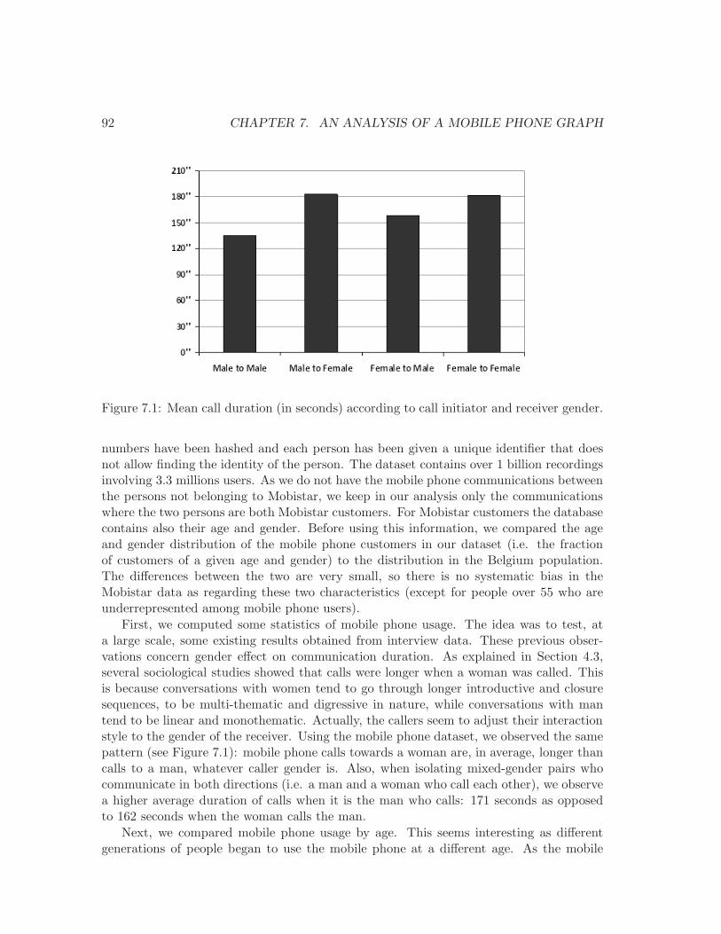
92 CHAPTER 7. AN ANALYSIS OF A MOBILE PHONE GRAPH
Figure 7.1: Mean call duration (in seconds) according to call initiator and receiver gender.
numbers have been hashed and each person has been given a unique identifier that doesnot allow finding the identity of the person. The dataset contains over 1 billion recordingsinvolving 3.3 millions users. As we do not have the mobile phone communications betweenthe persons not belonging to Mobistar, we keep in our analysis only the communicationswhere the two persons are both Mobistar customers. For Mobistar customers the databasecontains also their age and gender. Before using this information, we compared the ageand gender distribution of the mobile phone customers in our dataset (i.e. the fractionof customers of a given age and gender) to the distribution in the Belgium population.The differences between the two are very small, so there is no systematic bias in theMobistar data as regarding these two characteristics (except for people over 55 who areunderrepresented among mobile phone users).
First, we computed some statistics of mobile phone usage. The idea was to test, ata large scale, some existing results obtained from interview data. These previous obser-vations concern gender effect on communication duration. As explained in Section 4.3,several sociological studies showed that calls were longer when a woman was called. Thisis because conversations with women tend to go through longer introductive and closuresequences, to be multi-thematic and digressive in nature, while conversations with mantend to be linear and monothematic. Actually, the callers seem to adjust their interactionstyle to the gender of the receiver. Using the mobile phone dataset, we observed the samepattern (see Figure 7.1): mobile phone calls towards a woman are, in average, longer thancalls to a man, whatever caller gender is. Also, when isolating mixed-gender pairs whocommunicate in both directions (i.e. a man and a woman who call each other), we observea higher average duration of calls when it is the man who calls: 171 seconds as opposedto 162 seconds when the woman calls the man.
Next, we compared mobile phone usage by age. This seems interesting as differentgenerations of people began to use the mobile phone at a different age. As the mobile
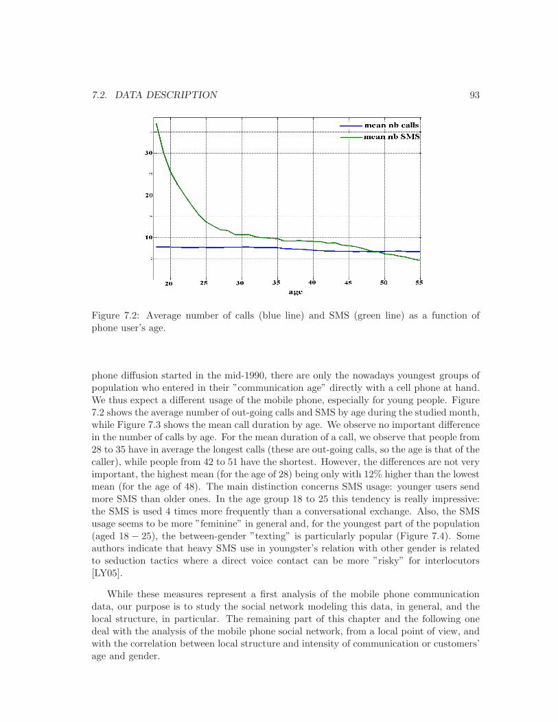
7.2. DATA DESCRIPTION 93
Figure 7.2: Average number of calls (blue line) and SMS (green line) as a function ofphone user’s age.
phone diffusion started in the mid-1990, there are only the nowadays youngest groups ofpopulation who entered in their ”communication age” directly with a cell phone at hand.We thus expect a different usage of the mobile phone, especially for young people. Figure7.2 shows the average number of out-going calls and SMS by age during the studied month,while Figure 7.3 shows the mean call duration by age. We observe no important differencein the number of calls by age. For the mean duration of a call, we observe that people from28 to 35 have in average the longest calls (these are out-going calls, so the age is that of thecaller), while people from 42 to 51 have the shortest. However, the differences are not veryimportant, the highest mean (for the age of 28) being only with 12% higher than the lowestmean (for the age of 48). The main distinction concerns SMS usage: younger users sendmore SMS than older ones. In the age group 18 to 25 this tendency is really impressive:the SMS is used 4 times more frequently than a conversational exchange. Also, the SMSusage seems to be more ”feminine” in general and, for the youngest part of the population(aged 18 − 25), the between-gender ”texting” is particularly popular (Figure 7.4). Someauthors indicate that heavy SMS use in youngster’s relation with other gender is relatedto seduction tactics where a direct voice contact can be more ”risky” for interlocutors[LY05].
While these measures represent a first analysis of the mobile phone communicationdata, our purpose is to study the social network modeling this data, in general, and thelocal structure, in particular. The remaining part of this chapter and the following onedeal with the analysis of the mobile phone social network, from a local point of view, andwith the correlation between local structure and intensity of communication or customers’age and gender.
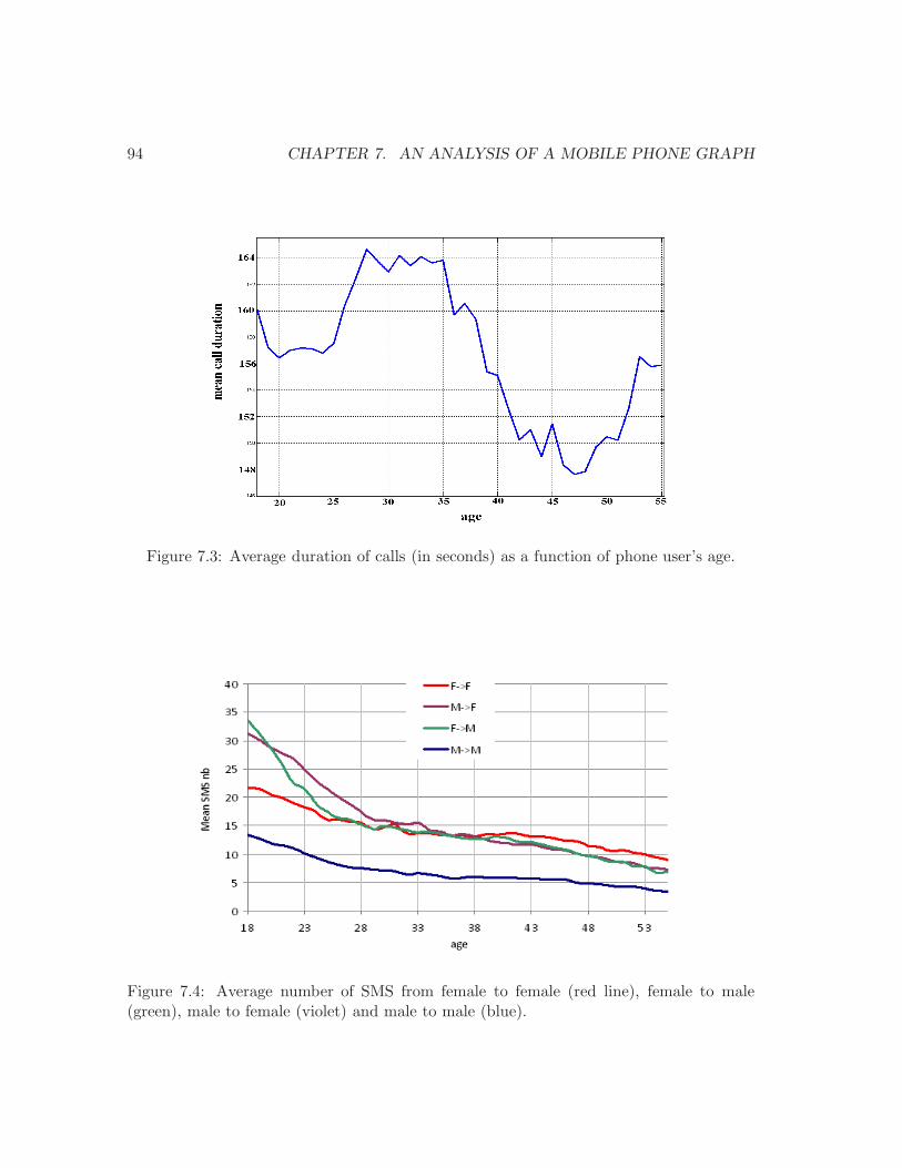
94 CHAPTER 7. AN ANALYSIS OF A MOBILE PHONE GRAPH
Figure 7.3: Average duration of calls (in seconds) as a function of phone user’s age.
Figure 7.4: Average number of SMS from female to female (red line), female to male(green), male to female (violet) and male to male (blue).
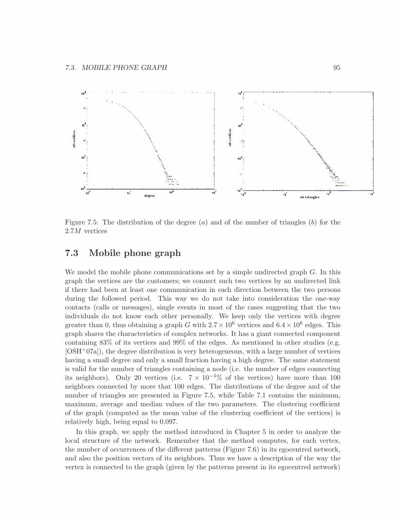
7.3. MOBILE PHONE GRAPH 95
Figure 7.5: The distribution of the degree (a) and of the number of triangles (b) for the2.7M vertices
7.3 Mobile phone graph
We model the mobile phone communications set by a simple undirected graph G. In thisgraph the vertices are the customers; we connect such two vertices by an undirected linkif there had been at least one communication in each direction between the two personsduring the followed period. This way we do not take into consideration the one-waycontacts (calls or messages), single events in most of the cases suggesting that the twoindividuals do not know each other personally. We keep only the vertices with degreegreater than 0, thus obtaining a graph G with 2.7× 10⁶ vertices and 6.4× 10⁶ edges. Thisgraph shares the characteristics of complex networks. It has a giant connected componentcontaining 83% of its vertices and 99% of the edges. As mentioned in other studies (e.g.[OSH+07a]), the degree distribution is very heterogeneous, with a large number of verticeshaving a small degree and only a small fraction having a high degree. The same statementis valid for the number of triangles containing a node (i.e. the number of edges connectingits neighbors). Only 20 vertices (i.e. 7 × 10⁻⁴% of the vertices) have more than 100neighbors connected by more that 100 edges. The distributions of the degree and of thenumber of triangles are presented in Figure 7.5, while Table 7.1 contains the minimum,maximum, average and median values of the two parameters. The clustering coefficientof the graph (computed as the mean value of the clustering coefficient of the vertices) isrelatively high, being equal to 0.097.
In this graph, we apply the method introduced in Chapter 5 in order to analyze thelocal structure of the network. Remember that the method computes, for each vertex,the number of occurrences of the different patterns (Figure 7.6) in its egocentred network,and also the position vectors of its neighbors. Thus we have a description of the way thevertex is connected to the graph (given by the patterns present in its egocentred network)
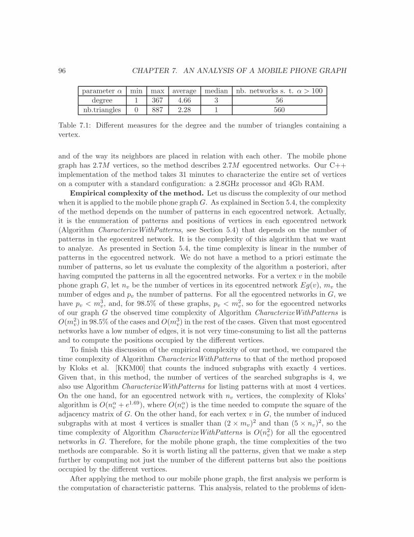
96 CHAPTER 7. AN ANALYSIS OF A MOBILE PHONE GRAPH
parameter α min max average median nb. networks s. t. α > 100
degree 1 367 4.66 3 56
nb.triangles 0 887 2.28 1 560
Table 7.1: Different measures for the degree and the number of triangles containing avertex.
and of the way its neighbors are placed in relation with each other. The mobile phonegraph has 2.7M vertices, so the method describes 2.7M egocentred networks. Our C++implementation of the method takes 31 minutes to characterize the entire set of verticeson a computer with a standard configuration: a 2.8GHz processor and 4Gb RAM.
Empirical complexity of the method. Let us discuss the complexity of our methodwhen it is applied to the mobile phone graphG. As explained in Section 5.4, the complexityof the method depends on the number of patterns in each egocentred network. Actually,it is the enumeration of patterns and positions of vertices in each egocentred network(Algorithm CharacterizeWithPatterns, see Section 5.4) that depends on the number ofpatterns in the egocentred network. It is the complexity of this algorithm that we wantto analyze. As presented in Section 5.4, the time complexity is linear in the number ofpatterns in the egocentred network. We do not have a method to a priori estimate thenumber of patterns, so let us evaluate the complexity of the algorithm a posteriori, afterhaving computed the patterns in all the egocentred networks. For a vertex v in the mobilephone graph G, let nv be the number of vertices in its egocentred network Eg(v), mv thenumber of edges and pv the number of patterns. For all the egocentred networks in G, wehave pv < m3
v, and, for 98.5% of these graphs, pv < m2v, so for the egocentred networks
of our graph G the observed time complexity of Algorithm CharacterizeWithPatterns isO(m2
v) in 98.5% of the cases and O(m3v) in the rest of the cases. Given that most egocentred
networks have a low number of edges, it is not very time-consuming to list all the patternsand to compute the positions occupied by the different vertices.
To finish this discussion of the empirical complexity of our method, we compared thetime complexity of Algorithm CharacterizeWithPatterns to that of the method proposedby Kloks et al. [KKM00] that counts the induced subgraphs with exactly 4 vertices.Given that, in this method, the number of vertices of the searched subgraphs is 4, wealso use Algorithm CharacterizeWithPatterns for listing patterns with at most 4 vertices.On the one hand, for an egocentred network with nv vertices, the complexity of Kloks’algorithm is O(nα
v + e1.69), where O(nαv ) is the time needed to compute the square of the
adjacency matrix of G. On the other hand, for each vertex v in G, the number of inducedsubgraphs with at most 4 vertices is smaller than (2 ×mv)
2 and than (5 × nv)2, so the
time complexity of Algorithm CharacterizeWithPatterns is O(n2v) for all the egocentred
networks in G. Therefore, for the mobile phone graph, the time complexities of the twomethods are comparable. So it is worth listing all the patterns, given that we make a stepfurther by computing not just the number of the different patterns but also the positionsoccupied by the different vertices.
After applying the method to our mobile phone graph, the first analysis we perform isthe computation of characteristic patterns. This analysis, related to the problems of iden-
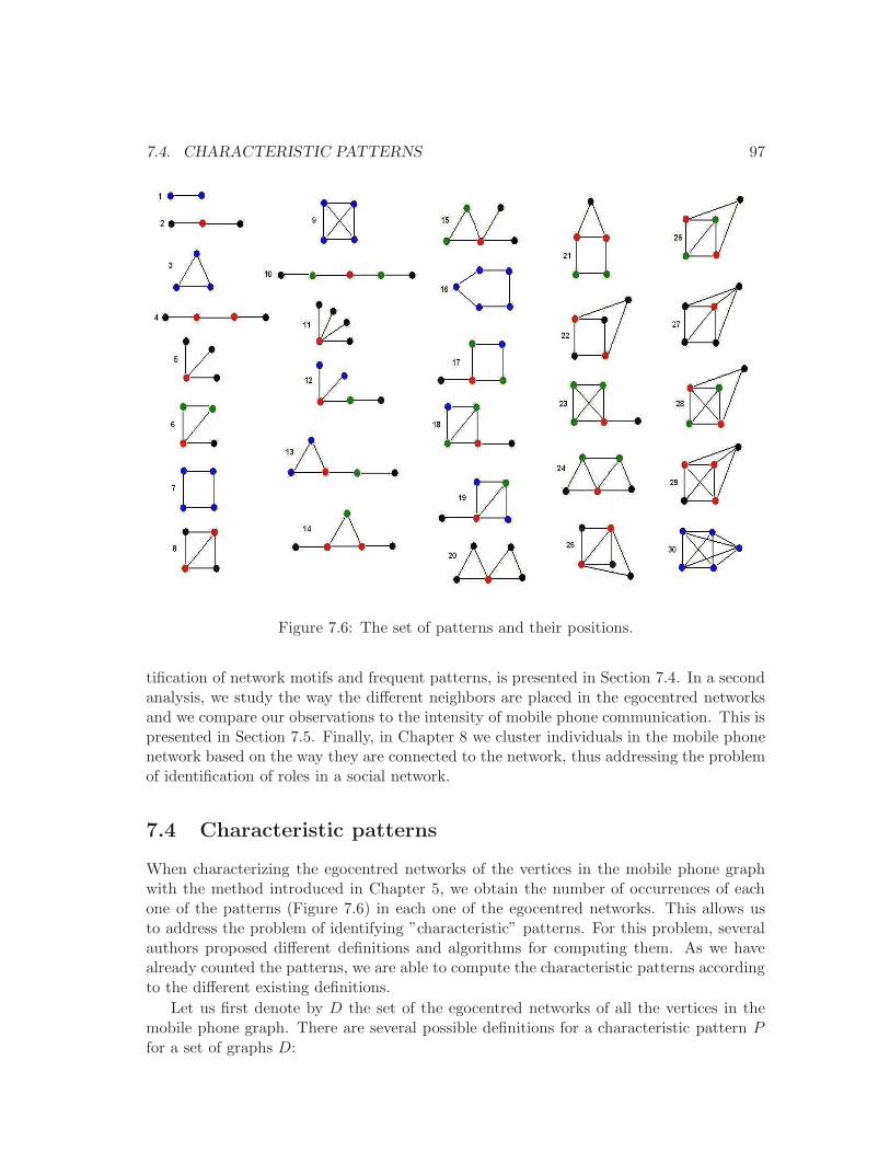
7.4. CHARACTERISTIC PATTERNS 97
Figure 7.6: The set of patterns and their positions.
tification of network motifs and frequent patterns, is presented in Section 7.4. In a secondanalysis, we study the way the different neighbors are placed in the egocentred networksand we compare our observations to the intensity of mobile phone communication. This ispresented in Section 7.5. Finally, in Chapter 8 we cluster individuals in the mobile phonenetwork based on the way they are connected to the network, thus addressing the problemof identification of roles in a social network.
7.4 Characteristic patterns
When characterizing the egocentred networks of the vertices in the mobile phone graphwith the method introduced in Chapter 5, we obtain the number of occurrences of eachone of the patterns (Figure 7.6) in each one of the egocentred networks. This allows usto address the problem of identifying ”characteristic” patterns. For this problem, severalauthors proposed different definitions and algorithms for computing them. As we havealready counted the patterns, we are able to compute the characteristic patterns accordingto the different existing definitions.
Let us first denote by D the set of the egocentred networks of all the vertices in themobile phone graph. There are several possible definitions for a characteristic pattern Pfor a set of graphs D:
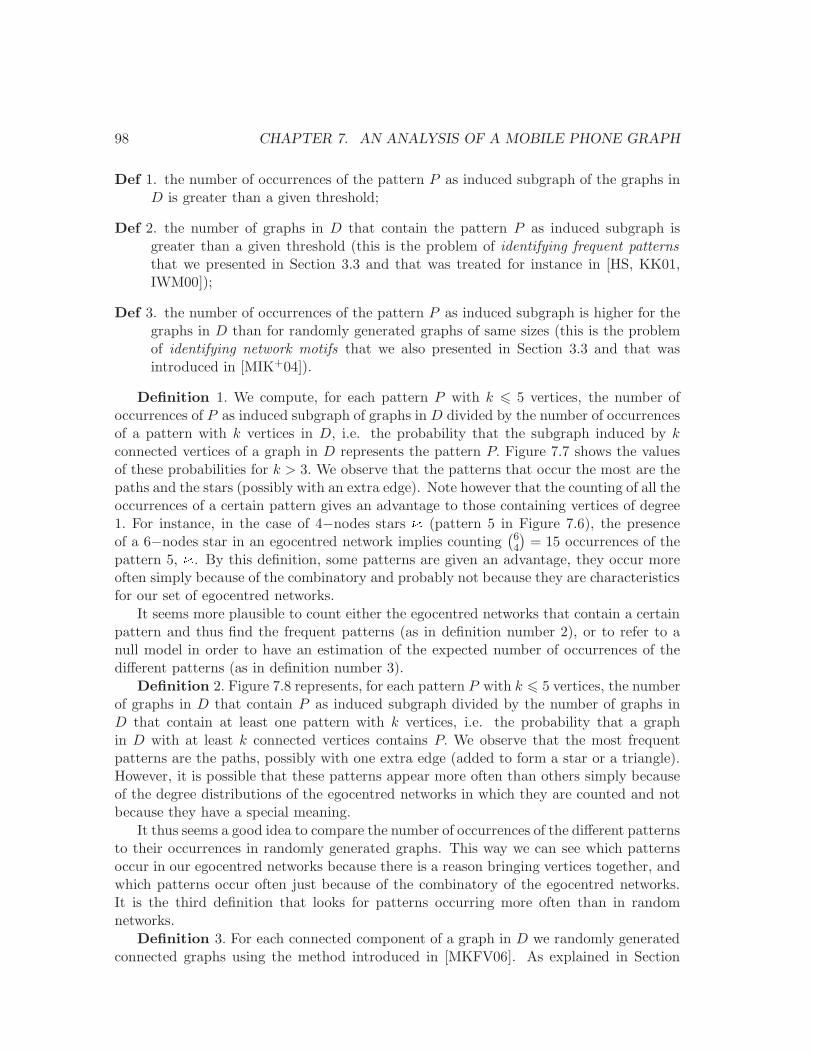
98 CHAPTER 7. AN ANALYSIS OF A MOBILE PHONE GRAPH
Def 1. the number of occurrences of the pattern P as induced subgraph of the graphs inD is greater than a given threshold;
Def 2. the number of graphs in D that contain the pattern P as induced subgraph isgreater than a given threshold (this is the problem of identifying frequent patternsthat we presented in Section 3.3 and that was treated for instance in [HS, KK01,IWM00]);
Def 3. the number of occurrences of the pattern P as induced subgraph is higher for thegraphs in D than for randomly generated graphs of same sizes (this is the problemof identifying network motifs that we also presented in Section 3.3 and that wasintroduced in [MIK+04]).
Definition 1. We compute, for each pattern P with k 6 5 vertices, the number ofoccurrences of P as induced subgraph of graphs in D divided by the number of occurrencesof a pattern with k vertices in D, i.e. the probability that the subgraph induced by kconnected vertices of a graph in D represents the pattern P. Figure 7.7 shows the valuesof these probabilities for k > 3. We observe that the patterns that occur the most are thepaths and the stars (possibly with an extra edge). Note however that the counting of all theoccurrences of a certain pattern gives an advantage to those containing vertices of degree1. For instance, in the case of 4−nodes stars (pattern 5 in Figure 7.6), the presenceof a 6−nodes star in an egocentred network implies counting
(64
)
= 15 occurrences of thepattern 5, . By this definition, some patterns are given an advantage, they occur moreoften simply because of the combinatory and probably not because they are characteristicsfor our set of egocentred networks.
It seems more plausible to count either the egocentred networks that contain a certainpattern and thus find the frequent patterns (as in definition number 2), or to refer to anull model in order to have an estimation of the expected number of occurrences of thedifferent patterns (as in definition number 3).
Definition 2. Figure 7.8 represents, for each pattern P with k 6 5 vertices, the numberof graphs in D that contain P as induced subgraph divided by the number of graphs inD that contain at least one pattern with k vertices, i.e. the probability that a graphin D with at least k connected vertices contains P. We observe that the most frequentpatterns are the paths, possibly with one extra edge (added to form a star or a triangle).However, it is possible that these patterns appear more often than others simply becauseof the degree distributions of the egocentred networks in which they are counted and notbecause they have a special meaning.
It thus seems a good idea to compare the number of occurrences of the different patternsto their occurrences in randomly generated graphs. This way we can see which patternsoccur in our egocentred networks because there is a reason bringing vertices together, andwhich patterns occur often just because of the combinatory of the egocentred networks.It is the third definition that looks for patterns occurring more often than in randomnetworks.
Definition 3. For each connected component of a graph in D we randomly generatedconnected graphs using the method introduced in [MKFV06]. As explained in Section
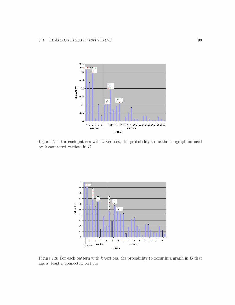
7.4. CHARACTERISTIC PATTERNS 99
Figure 7.7: For each pattern with k vertices, the probability to be the subgraph inducedby k connected vertices in D
Figure 7.8: For each pattern with k vertices, the probability to occur in a graph in D thathas at least k connected vertices
100 CHAPTER 7. AN ANALYSIS OF A MOBILE PHONE GRAPH
3.2, this method uses dK−series of probability distributions (i.e. all degree correlationswithin d−sized subgraphs). We built graphs for d = 1, 2 and 3 respectively. For d = 1,the generated graphs preserve the degree distribution of the original graphs, thus assuringalso the same number of vertices and edges. For d = 2, the joint degree distribution ispreserved, thus keeping also the same degree distribution. For d = 3, the graph generationpreserves the number of triangles and wedges (i.e. chains of 3 vertices connected by 2 edges)between vertices with degrees k1, k2, k3, ∀k1, k2, k3 ∈ N.
For each value of d, let Rd be the set of randomly generated graphs. For each pattern,we compute the ratio between its number of occurrences in the graphs in D and in thegraphs in Rd. When the graphs in D are compared to the graphs in Rd, the patternswith the greatest values of the ratios are characteristic for the graphs in D and the oneswith the smallest values are underrepresented. For d = 1 and d = 2, the same patternsare identified as characteristic (see Figure 7.9), with smaller values of the ratio for d = 2than for d = 1. These patterns suggest that, although the densities of the input graphsare preserved in the generated ones, there are graphs in D that are locally denser thanthe corresponding generated ones. So, in the neighborhood of certain vertices, severalneighbors form dense clusters; these clusters may correspond to the different groups ofcontacts of those persons. Note however that the two generations preserve the clusteringcoefficients of the graphs in D. When k = 3, the clustering coefficient is preserved (alongwith some other conditions, see Section 3.2) and the observed values of the ratio are placedbetween 0.99 and 1.003 for all the patterns. The generated graphs essentially reconstructthe original ones, so the 3k−distribution suffices in order to capture the distributions ofthe different patterns in the neighborhood graphs in GM. Nevertheless, this generation isvery constraining for small graphs like those in D; in many cases there is only one graphthat has the 3k−distribution of the original one: the original one.
To sum up, computing characteristics patterns is not an easy job. Each one of thedefinitions has its limitations. Even if the third definition seems the most useful, themethod for graph generation influences a lot the results; the characteristic patterns foundby using a certain graph generation method may not appear as characteristic if one changesthe method.
7.5 A characterization of ego’s contacts
By applying the method local structure described in Chapter 5 to each vertex (also calledego) v of the mobile phone graph, we obtain a description of how the neighbors of thevertex are placed in relation to each other. This description is a vector, called positionvector, computed for each one of the neighbors u of the vertex v. It contains the numberof occurrences of u in the different positions of the patterns identified in the egocentrednetwork of v (Figure 7.6 represents the patterns and their positions; in each pattern eachposition has a different color). We want to see if there is a relation between the featurevectors of the different neighbors, so between their positions in the egocentred network,and the intensity of their communication with v. We thus compare the position vectors tothe number of calls with v and to the total duration of calls. Note that the position vectors
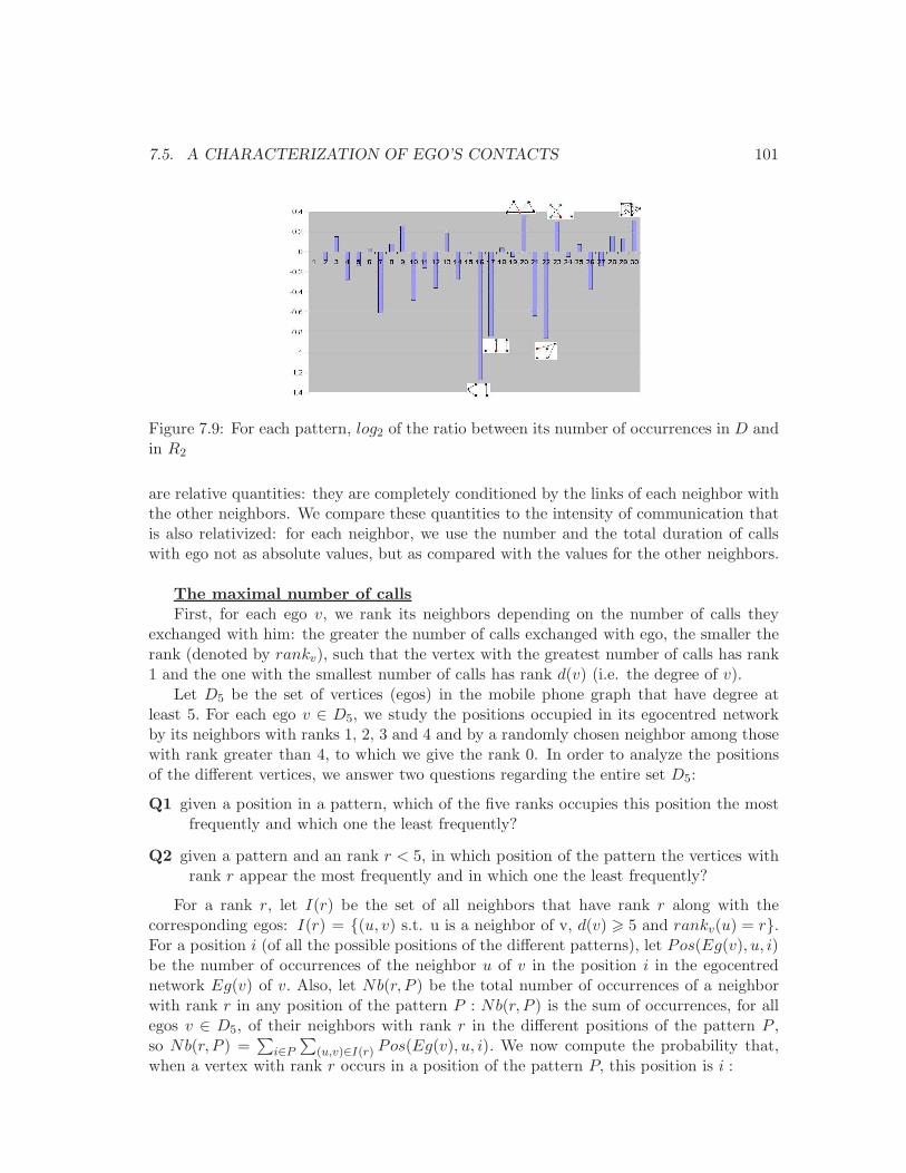
7.5. A CHARACTERIZATION OF EGO’S CONTACTS 101
Figure 7.9: For each pattern, log2 of the ratio between its number of occurrences in D andin R2
are relative quantities: they are completely conditioned by the links of each neighbor withthe other neighbors. We compare these quantities to the intensity of communication thatis also relativized: for each neighbor, we use the number and the total duration of callswith ego not as absolute values, but as compared with the values for the other neighbors.
The maximal number of callsFirst, for each ego v, we rank its neighbors depending on the number of calls they
exchanged with him: the greater the number of calls exchanged with ego, the smaller therank (denoted by rankv), such that the vertex with the greatest number of calls has rank1 and the one with the smallest number of calls has rank d(v) (i.e. the degree of v).
Let D5 be the set of vertices (egos) in the mobile phone graph that have degree atleast 5. For each ego v ∈ D5, we study the positions occupied in its egocentred networkby its neighbors with ranks 1, 2, 3 and 4 and by a randomly chosen neighbor among thosewith rank greater than 4, to which we give the rank 0. In order to analyze the positionsof the different vertices, we answer two questions regarding the entire set D5:
Q1 given a position in a pattern, which of the five ranks occupies this position the mostfrequently and which one the least frequently?
Q2 given a pattern and an rank r < 5, in which position of the pattern the vertices withrank r appear the most frequently and in which one the least frequently?
For a rank r, let I(r) be the set of all neighbors that have rank r along with thecorresponding egos: I(r) = {(u, v) s.t. u is a neighbor of v, d(v) > 5 and rankv(u) = r}.For a position i (of all the possible positions of the different patterns), let Pos(Eg(v), u, i)be the number of occurrences of the neighbor u of v in the position i in the egocentrednetwork Eg(v) of v. Also, let Nb(r, P ) be the total number of occurrences of a neighborwith rank r in any position of the pattern P : Nb(r, P ) is the sum of occurrences, for allegos v ∈ D5, of their neighbors with rank r in the different positions of the pattern P ,so Nb(r, P ) =
∑
i∈P
∑
(u,v)∈I(r) Pos(Eg(v), u, i). We now compute the probability that,when a vertex with rank r occurs in a position of the pattern P, this position is i :
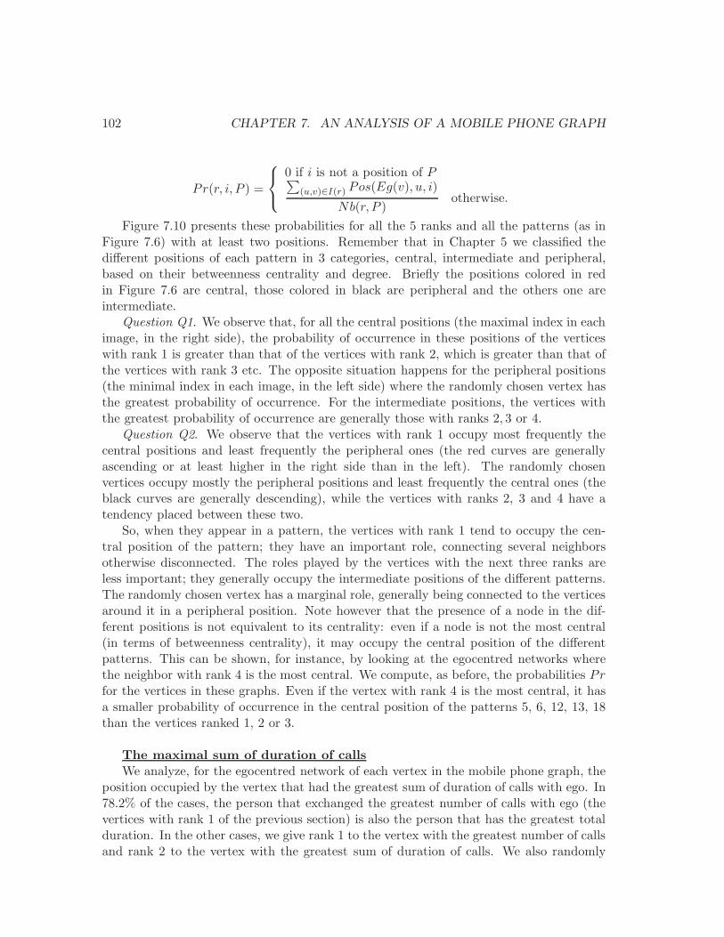
102 CHAPTER 7. AN ANALYSIS OF A MOBILE PHONE GRAPH
Pr(r, i, P ) =
0 if i is not a position of P∑
(u,v)∈I(r) Pos(Eg(v), u, i)
Nb(r, P )otherwise.
Figure 7.10 presents these probabilities for all the 5 ranks and all the patterns (as inFigure 7.6) with at least two positions. Remember that in Chapter 5 we classified thedifferent positions of each pattern in 3 categories, central, intermediate and peripheral,based on their betweenness centrality and degree. Briefly the positions colored in redin Figure 7.6 are central, those colored in black are peripheral and the others one areintermediate.
Question Q1. We observe that, for all the central positions (the maximal index in eachimage, in the right side), the probability of occurrence in these positions of the verticeswith rank 1 is greater than that of the vertices with rank 2, which is greater than that ofthe vertices with rank 3 etc. The opposite situation happens for the peripheral positions(the minimal index in each image, in the left side) where the randomly chosen vertex hasthe greatest probability of occurrence. For the intermediate positions, the vertices withthe greatest probability of occurrence are generally those with ranks 2, 3 or 4.
Question Q2. We observe that the vertices with rank 1 occupy most frequently thecentral positions and least frequently the peripheral ones (the red curves are generallyascending or at least higher in the right side than in the left). The randomly chosenvertices occupy mostly the peripheral positions and least frequently the central ones (theblack curves are generally descending), while the vertices with ranks 2, 3 and 4 have atendency placed between these two.
So, when they appear in a pattern, the vertices with rank 1 tend to occupy the cen-tral position of the pattern; they have an important role, connecting several neighborsotherwise disconnected. The roles played by the vertices with the next three ranks areless important; they generally occupy the intermediate positions of the different patterns.The randomly chosen vertex has a marginal role, generally being connected to the verticesaround it in a peripheral position. Note however that the presence of a node in the dif-ferent positions is not equivalent to its centrality: even if a node is not the most central(in terms of betweenness centrality), it may occupy the central position of the differentpatterns. This can be shown, for instance, by looking at the egocentred networks wherethe neighbor with rank 4 is the most central. We compute, as before, the probabilities Prfor the vertices in these graphs. Even if the vertex with rank 4 is the most central, it hasa smaller probability of occurrence in the central position of the patterns 5, 6, 12, 13, 18than the vertices ranked 1, 2 or 3.
The maximal sum of duration of callsWe analyze, for the egocentred network of each vertex in the mobile phone graph, the
position occupied by the vertex that had the greatest sum of duration of calls with ego. In78.2% of the cases, the person that exchanged the greatest number of calls with ego (thevertices with rank 1 of the previous section) is also the person that has the greatest totalduration. In the other cases, we give rank 1 to the vertex with the greatest number of callsand rank 2 to the vertex with the greatest sum of duration of calls. We also randomly
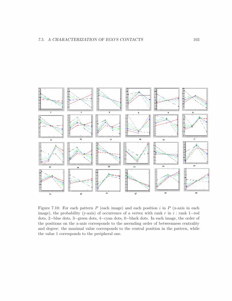
7.5. A CHARACTERIZATION OF EGO’S CONTACTS 103
Figure 7.10: For each pattern P (each image) and each position i in P (x-axis in eachimage), the probability (y-axis) of occurrence of a vertex with rank r in i : rank 1−reddots, 2−blue dots, 3−green dots, 4−cyan dots, 0−black dots. In each image, the order ofthe positions on the x-axis corresponds to the ascending order of betweenness centralityand degree: the maximal value corresponds to the central position in the pattern, whilethe value 1 corresponds to the peripheral one.
104 CHAPTER 7. AN ANALYSIS OF A MOBILE PHONE GRAPH
choose a vertex among the other neighbors of ego. By performing a similar analysis to thatof the previous section, we observe, for each pattern, that the probability of the verticeswith rank 2 to occupy the central position is smaller than that of the vertices with rank 1but higher than that of the randomly chosen vertices. The opposite situation happens forthe peripheral positions. When they appear in a pattern, the vertices with rank 2 tend tooccupy the intermediate positions.
Comments on the results
Our data provides us two measures of the intensity of communications between eachego and his neighbors: the frequency and the duration of calls. It seems intuitive thatthe person who speaks the most with ego has an important role in his network. However,when it is not the same person that has the greatest frequency of calls and the greatestduration, it is interesting to see which of the two actors has a more important role in ego’sneighborhood. Using the number of occurrences in the different positions, we saw that itis the one that has the greatest frequency who has a more important role.
Remeber that in Section 4.3 we presented a sociological study by Licoppe and Smoredaon phone communications [LS05]. In this study the authors, using databases of telephonecalls and several interviews focusing on the use of telephone, identified two patterns ofcommunication, the ”connected presence” and the ”intermittent presence”. In the firstone, the two persons, socially and often also geographically close, are frequently in contactwith each other, exchanging many short calls and messages. They share activities thatrequire numerous calls for synchronization and coordination, the mobile phone being espe-cially suitable for this. It seems plausible that the persons that speak the most frequentlywith ego are well involved in ego’s network, being well connected to other neighbors. In-deed, we saw that the actors that communicate the most with ego tend to occupy thecentral positions of the patterns where they appear.
In the second pattern identified by Licoppe and Smoreda, the two persons, close friendsor intimate relatives, are not able to see each other or talk very often. Their conversationsare long, they give and receive news, trying to compensate for the rarity of face-to-facecontacts. The person that has long but rare calls with ego is probably geographically farfrom him, while the persons that have a great frequency of calls are generally geographicallyclose. This hypothesis is confirmed in [LBdK+08], where Lambiotte et al. show that theprobability of a mobile phone call between two persons is inversely proportional to thesquare of the geographical distance between them. Being far from ego, the person thathas the greatest duration of calls but not the greatest frequency is less implied in ego’snetwork, his role is less important. However, the duration of the calls suggests that heis sociologically close to ego, hence his more important position than that of a randomlychosen neighbor.
7.6 Chapter conclusions
In this chapter we presented an analysis of a dataset of mobile phone communications.We first computed some statistics of phone usage and then we analyzed the local structure
7.6. CHAPTER CONCLUSIONS 105
of the graph by using the method introduced in Chapter 5. Until now we addressed thequestion of computing the characteristics patterns of the egocentred networks, thus relatingto some very popular problems in pattern discovery, data mining and bio-informatics.Next we analyzed the positions occupied by the neighbors of each vertex in its egocentrednetwork, thus addressing the notion of the roles played by the different vertices in theegocentred network. When we compared the relative positions of the neighbors to theintensity of communications with ego, we found that the person who had a great frequencyof calls with ego had, in average, an important position in its egocentred network. Thisposition is generally more important than that of the person who has the greatest durationof calls with ego.
In the next chapter we group together vertices having similar egocentred networksand we confront the different groups to the quantity of communications and to the socio-demographic data.

106 CHAPTER 7. AN ANALYSIS OF A MOBILE PHONE GRAPH
Chapter 8
A local structure-based clusteringof nodes
8.1 Introduction
Remember that, for each individual in the mobile phone network, we listed the patternsof his egocentred network. The number of occurrences of the different patterns representsa description of how each node (so each individual) is connected to the network. In thischapter, we use this description in order to group individuals into clusters: nodes are putin the same cluster because they are connected to the network in similar ways; nodes putin distinct clusters are differently embedded in the network. One can see this distributionof nodes into clusters as an identification of roles played in the network, as presented inSection 4.1.1. Without pretending to have solved the problem of identification of roles,we present a method to distribute nodes into clusters based on the local structure of thenetwork. We use the k-pattern vectors that we have defined in Section 5.3, but in a differentway than in the definition of the k-pattern equivalence (that we have also introduced inSection 5.3).
There are of course many ways of clustering nodes of a network, but the methodwe propose here gives quite promising results, in particular when they are confronted toother characteristics of the individuals. Indeed the probability that an individual belongsto a certain cluster depends on his age; even more, using these probabilities we are ableto group together different ages, thus discovering 4 groups containing consecutive ages,corresponding to 4 life stages. The probability that a person belongs to a certain clusteralso depends on his mobile phone communication intensity; moreover the intensity ofcommunication allows us to predict with rather high accuracy the cluster a person belongsto.
We begin by presenting the method for grouping nodes into clusters based on thestructure of the network in which they are embedded. We then confront the obtainedclusters to age, gender and intensity of communication. We finally provide a typologyof the mobile phone users in our dataset based on social network cluster, intensity ofcommunications and socio-demographic data.
107
108 CHAPTER 8. A LOCAL STRUCTURE-BASED CLUSTERING OF NODES
8.2 A method for nodes clustering using patterns frequency
In this section we want to group together the vertices of a given large graph G which areconnected in the same way to the network. This is the problem of identification of socialroles that we presented in Section 4.1.1.
8.2.1 Pattern-frequency equivalence
Generally, when computing roles of nodes in a network one defines an equivalence relationbetween nodes: equivalent nodes are considered to have the same role. In Section 5.3 wehave defined such an equivalence relation called k-pattern equivalence. This relation isbased on k-pattern vectors. We recall the two definitions here.
Definition 8.2.1. Given a vertex v of a graph G and a positive integer k, we call k-patternvector of v the vector containing the number of occurrences of the k-patterns (i.e. all thenon-isomorphic connected graphs with at most k vertices) in the egocentred network Eg(v)of v. Two vertices of the graph G are said to be k-pattern equivalent if and only if theyhave identical k-pattern vectors.
Although the k-pattern equivalence is less strict than the structural and the automor-phic equivalences (as explained in Section 5.6), it is still not flexible enough for real-worldnetworks. The problem is that the equivalence classes obtained when applying the def-inition to large graphs are much too numerous. Here we want to group the nodes of agiven large network into a small number of classes (i.e. smaller than a given constant,for instance 20). Each class should contain similar nodes in terms of network structure.It is the local structure of the network surrounding the node that should matter whenattributing a node to a class, and not its degree or the fact of being connected to othernodes in the class. The interest of computing such classes is that they are very easy to use.Thus, one can measure correlations with other properties of the nodes or make predictions(e.g. predict a property when knowing the class and vice-versa).
One possible solution is to characterize each vertex of the given graph G by a vectorwith n components and then to define an equivalence relation of vectors (and thus obtainan equivalence relation of vertices).
Definition 8.2.2. Given a graph G = (V,E), a characterization function f : V → Rn
and a relation r ∈ Rn ×R
n, two vertices u, v ∈ V are said to be r-equivalent if and only ifone has (f(u), f(v)) ∈ r.
If one takes for instance, for each vertex v of the graph G, f(v) to be the k-patternvector of v and r to be the identity, one has that two vertices u and v of G are r-equivalentif and only if they are k-pattern equivalent.
In order to define a r-equivalence on the vertices of a graph G, one has to give adefinition of characterization function f and of relation r. Here, we base our definition ofcharacterization function on 4-pattern vectors. As for the relation r, we define it using aclustering method that we introduce.
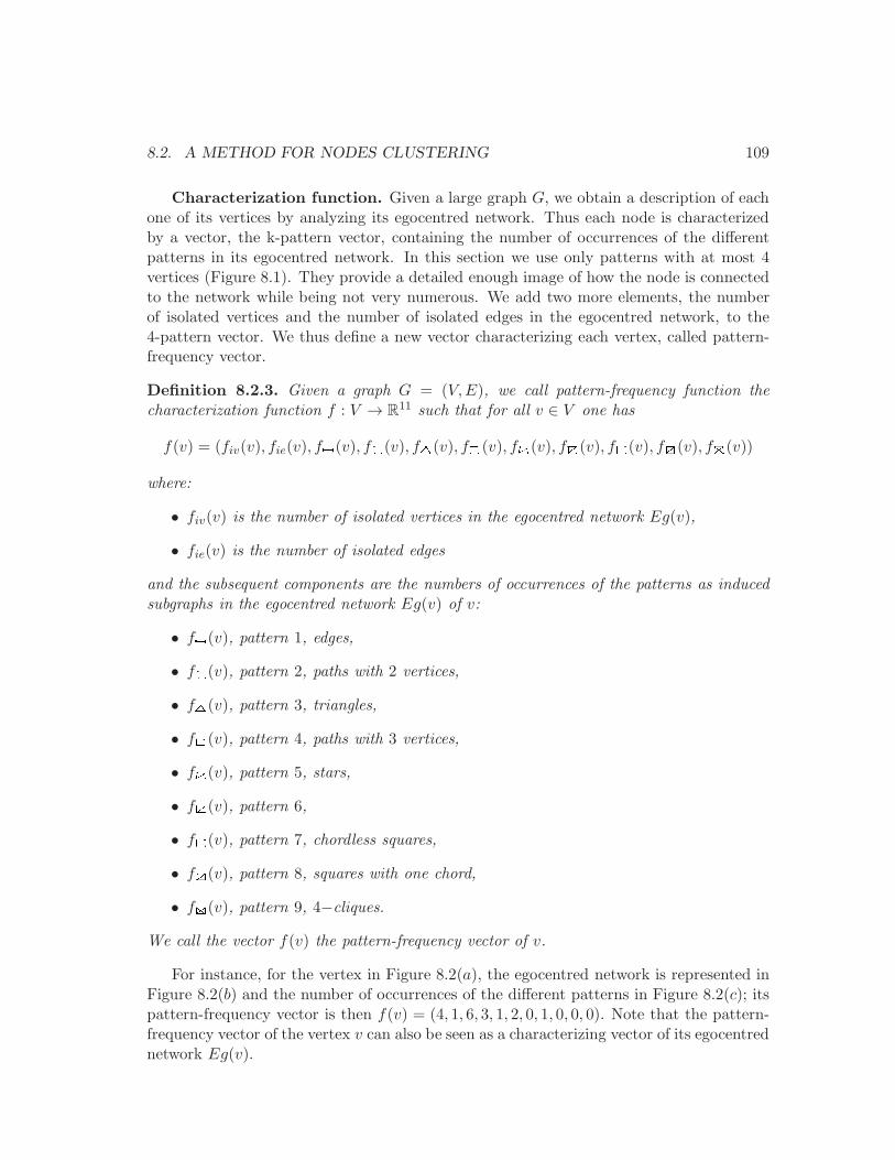
8.2. A METHOD FOR NODES CLUSTERING 109
Characterization function. Given a large graph G, we obtain a description of eachone of its vertices by analyzing its egocentred network. Thus each node is characterizedby a vector, the k-pattern vector, containing the number of occurrences of the differentpatterns in its egocentred network. In this section we use only patterns with at most 4vertices (Figure 8.1). They provide a detailed enough image of how the node is connectedto the network while being not very numerous. We add two more elements, the numberof isolated vertices and the number of isolated edges in the egocentred network, to the4-pattern vector. We thus define a new vector characterizing each vertex, called pattern-frequency vector.
Definition 8.2.3. Given a graph G = (V,E), we call pattern-frequency function thecharacterization function f : V → R
11 such that for all v ∈ V one has
f(v) = (fiv(v), fie(v), f (v), f (v), f (v), f (v), f (v), f (v), f (v), f (v), f (v))
where:
• fiv(v) is the number of isolated vertices in the egocentred network Eg(v),
• fie(v) is the number of isolated edges
and the subsequent components are the numbers of occurrences of the patterns as inducedsubgraphs in the egocentred network Eg(v) of v:
• f (v), pattern 1, edges,
• f (v), pattern 2, paths with 2 vertices,
• f (v), pattern 3, triangles,
• f (v), pattern 4, paths with 3 vertices,
• f (v), pattern 5, stars,
• f (v), pattern 6,
• f (v), pattern 7, chordless squares,
• f (v), pattern 8, squares with one chord,
• f (v), pattern 9, 4−cliques.
We call the vector f(v) the pattern-frequency vector of v.
For instance, for the vertex in Figure 8.2(a), the egocentred network is represented inFigure 8.2(b) and the number of occurrences of the different patterns in Figure 8.2(c); itspattern-frequency vector is then f(v) = (4, 1, 6, 3, 1, 2, 0, 1, 0, 0, 0). Note that the pattern-frequency vector of the vertex v can also be seen as a characterizing vector of its egocentrednetwork Eg(v).
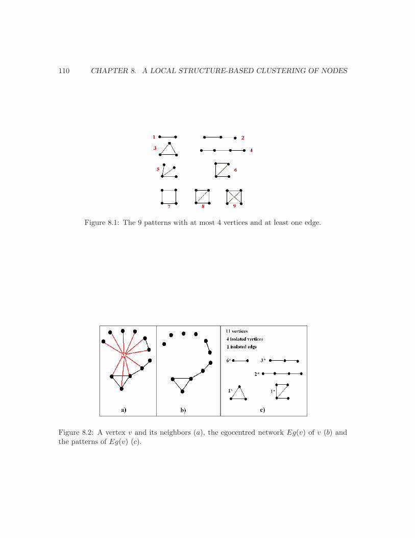
110 CHAPTER 8. A LOCAL STRUCTURE-BASED CLUSTERING OF NODES
Figure 8.1: The 9 patterns with at most 4 vertices and at least one edge.
Figure 8.2: A vertex v and its neighbors (a), the egocentred network Eg(v) of v (b) andthe patterns of Eg(v) (c).
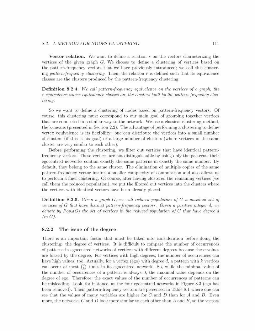
8.2. A METHOD FOR NODES CLUSTERING 111
Vector relation. We want to define a relation r on the vectors characterizing thevertices of the given graph G. We choose to define a clustering of vertices based onthe pattern-frequency vectors that we have previously introduced; we call this cluster-ing pattern-frequency clustering. Then, the relation r is defined such that its equivalenceclasses are the clusters produced by the pattern-frequency clustering.
Definition 8.2.4. We call pattern-frequency equivalence on the vertices of a graph, ther-equivalence whose equivalence classes are the clusters built by the pattern-frequency clus-tering.
So we want to define a clustering of nodes based on pattern-frequency vectors. Ofcourse, this clustering must correspond to our main goal of grouping together verticesthat are connected in a similar way to the network. We use a classical clustering method,the k-means (presented in Section 2.2). The advantage of performing a clustering to definevertex equivalence is its flexibility: one can distribute the vertices into a small numberof clusters (if this is his goal) or a large number of clusters (where vertices in the samecluster are very similar to each other).
Before performing the clustering, we filter out vertices that have identical pattern-frequency vectors. These vertices are not distinguishable by using only the patterns; theiregocentred networks contain exactly the same patterns in exactly the same number. Bydefault, they belong to the same cluster. The elimination of multiple copies of the samepattern-frequency vector insures a smaller complexity of computation and also allows usto perform a finer clustering. Of course, after having clustered the remaining vertices (wecall them the reduced population), we put the filtered out vertices into the clusters wherethe vertices with identical vectors have been already placed.
Definition 8.2.5. Given a graph G, we call reduced population of G a maximal set ofvertices of G that have distinct pattern-frequency vectors. Given a positive integer d, wedenote by Popd(G) the set of vertices in the reduced population of G that have degree d(in G).
8.2.2 The issue of the degree
There is an important factor that must be taken into consideration before doing theclustering: the degree of vertices. It is difficult to compare the number of occurrencesof patterns in egocentred networks of vertices with different degrees because these valuesare biased by the degree. For vertices with high degrees, the number of occurrences canhave high values, too. Actually, for a vertex (ego) with degree d, a pattern with k verticescan occur at most
(
dk
)
times in its egocentred network. So, while the minimal value ofthe number of occurrences of a pattern is always 0, the maximal value depends on thedegree of ego. Therefore, the exact values of the number of occurrences of patterns canbe misleading. Look, for instance, at the four egocentred networks in Figure 8.3 (ego hasbeen removed). Their pattern-frequency vectors are presented in Table 8.1 where one cansee that the values of many variables are higher for C and D than for A and B. Evenmore, the networks C and D look more similar to each other than A and B, so the vectors
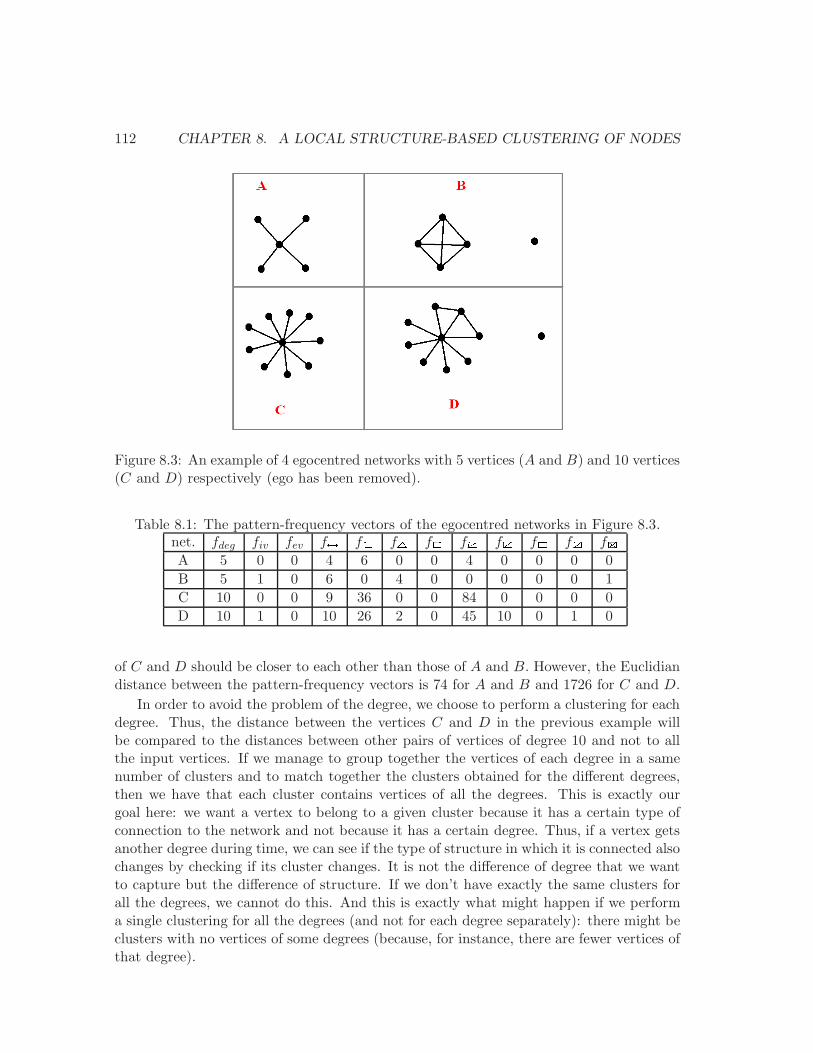
112 CHAPTER 8. A LOCAL STRUCTURE-BASED CLUSTERING OF NODES
Figure 8.3: An example of 4 egocentred networks with 5 vertices (A and B) and 10 vertices(C and D) respectively (ego has been removed).
Table 8.1: The pattern-frequency vectors of the egocentred networks in Figure 8.3.net. fdeg fiv fev f f f f f f f f f
A 5 0 0 4 6 0 0 4 0 0 0 0
B 5 1 0 6 0 4 0 0 0 0 0 1
C 10 0 0 9 36 0 0 84 0 0 0 0
D 10 1 0 10 26 2 0 45 10 0 1 0
of C and D should be closer to each other than those of A and B. However, the Euclidiandistance between the pattern-frequency vectors is 74 for A and B and 1726 for C and D.
In order to avoid the problem of the degree, we choose to perform a clustering for eachdegree. Thus, the distance between the vertices C and D in the previous example willbe compared to the distances between other pairs of vertices of degree 10 and not to allthe input vertices. If we manage to group together the vertices of each degree in a samenumber of clusters and to match together the clusters obtained for the different degrees,then we have that each cluster contains vertices of all the degrees. This is exactly ourgoal here: we want a vertex to belong to a given cluster because it has a certain type ofconnection to the network and not because it has a certain degree. Thus, if a vertex getsanother degree during time, we can see if the type of structure in which it is connected alsochanges by checking if its cluster changes. It is not the difference of degree that we wantto capture but the difference of structure. If we don’t have exactly the same clusters forall the degrees, we cannot do this. And this is exactly what might happen if we performa single clustering for all the degrees (and not for each degree separately): there might beclusters with no vertices of some degrees (because, for instance, there are fewer vertices ofthat degree).
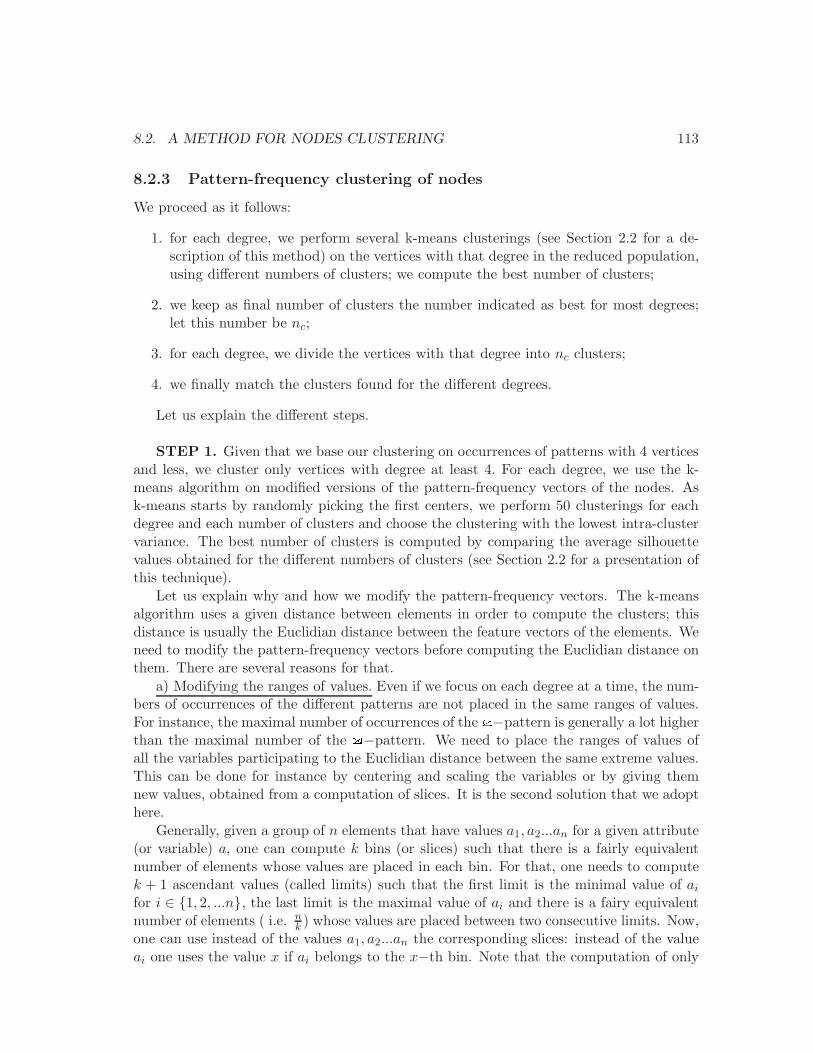
8.2. A METHOD FOR NODES CLUSTERING 113
8.2.3 Pattern-frequency clustering of nodes
We proceed as it follows:
1. for each degree, we perform several k-means clusterings (see Section 2.2 for a de-scription of this method) on the vertices with that degree in the reduced population,using different numbers of clusters; we compute the best number of clusters;
2. we keep as final number of clusters the number indicated as best for most degrees;let this number be nc;
3. for each degree, we divide the vertices with that degree into nc clusters;
4. we finally match the clusters found for the different degrees.
Let us explain the different steps.
STEP 1. Given that we base our clustering on occurrences of patterns with 4 verticesand less, we cluster only vertices with degree at least 4. For each degree, we use the k-means algorithm on modified versions of the pattern-frequency vectors of the nodes. Ask-means starts by randomly picking the first centers, we perform 50 clusterings for eachdegree and each number of clusters and choose the clustering with the lowest intra-clustervariance. The best number of clusters is computed by comparing the average silhouettevalues obtained for the different numbers of clusters (see Section 2.2 for a presentation ofthis technique).
Let us explain why and how we modify the pattern-frequency vectors. The k-meansalgorithm uses a given distance between elements in order to compute the clusters; thisdistance is usually the Euclidian distance between the feature vectors of the elements. Weneed to modify the pattern-frequency vectors before computing the Euclidian distance onthem. There are several reasons for that.
a) Modifying the ranges of values. Even if we focus on each degree at a time, the num-bers of occurrences of the different patterns are not placed in the same ranges of values.For instance, the maximal number of occurrences of the −pattern is generally a lot higherthan the maximal number of the −pattern. We need to place the ranges of values ofall the variables participating to the Euclidian distance between the same extreme values.This can be done for instance by centering and scaling the variables or by giving themnew values, obtained from a computation of slices. It is the second solution that we adopthere.
Generally, given a group of n elements that have values a1, a2...an for a given attribute(or variable) a, one can compute k bins (or slices) such that there is a fairly equivalentnumber of elements whose values are placed in each bin. For that, one needs to computek + 1 ascendant values (called limits) such that the first limit is the minimal value of aifor i ∈ {1, 2, ...n}, the last limit is the maximal value of ai and there is a fairy equivalentnumber of elements ( i.e. n
k) whose values are placed between two consecutive limits. Now,
one can use instead of the values a1, a2...an the corresponding slices: instead of the valueai one uses the value x if ai belongs to the x−th bin. Note that the computation of only
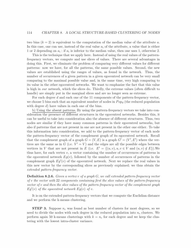
114 CHAPTER 8. A LOCAL STRUCTURE-BASED CLUSTERING OF NODES
two bins (k = 2) is equivalent to the computation of the median value of the attribute a.In this case, one can use, instead of the real value ai of the attribute, a value that is either1 or 2 depending on ai : if ai is inferior to the median value, then one uses 1, otherwise 2.
This is the technique that we apply here. Instead of using the real values of the pattern-frequency vectors, we compute and use slices of values. There are several advantages indoing this. First, we eliminate the problem of comparing very different values for differentpatterns: now we have, for all the patterns, the same possible values. Second, the newvalues are established using the ranges of values, as found in the network. Thus, thenumber of occurrences of a given pattern in a given egocentred network can be very smallcomparing to the maximal possible value and, in the same time, very high comparing toits value in the other egocentred networks. We want to emphasize the fact that this valueis high in our network, which the slices do. Thirdly, the extreme values (often difficult tohandle) are simply put in the marginal slices and are no longer seen as extreme.
For each degree d and each one of the 11 components of the pattern-frequency vector,we choose 5 bins such that an equivalent number of nodes in Popd (the reduced populationwith degree d) have values in each one of the bins.
b) Using the absent patterns. By using the pattern-frequency vectors we take into con-sideration the presence of different structures in the egocentred networks. Besides this, itcan be useful to take into consideration also the absence of different structures. Thus, twonodes are similar if they have many common patterns in their egocentred networks, butalso if patterns that are not present in one are not present in the other one either. To takethis information into consideration, we add to the pattern-frequency vector of each nodethe pattern-frequency vector of the complement graph of its egocentred network. Recallthat the complement graph of a graph G = (V,E) is a graph G′ = (V ′, E′) where the ver-tices are the same as in G (i.e. V ′ = V ) and the edges are all the possible edges betweenvertices in V that are not present in E (i.e. E′ = {(u, v), u, v ∈ V and (u, v) /∈ E}).Wethus have, for each vertex v, a vector containing the number of occurrences of patterns inthe egocentred network Eg(v), followed by the number of occurrences of patterns in thecomplement graph Eg′(v) of the egocentred network. Next we replace the real values inthis new vector by the corresponding slices as previously explained; we thus obtain theextended pattern-frequency vector.
Definition 8.2.6. Given a vertex v of a graph G, we call extended pattern-frequency vectorof v the vector with 22 components containing first the slice values of the pattern-frequencyvector of v and then the slice values of the pattern-frequency vector of the complement graphEg′(v) of the egocentred network Eg(v) of v.
It is on the extended pattern-frequency vectors that we compute the Euclidian distanceand we perform the k-means clustering.
STEP 3. Suppose nc was found as best number of clusters for most degrees, so weneed to divide the nodes with each degree in the reduced population into nc clusters. Weperform again 50 k-means clusterings with k = nc for each degree and we keep the clus-tering with the lowest intra-cluster variance.
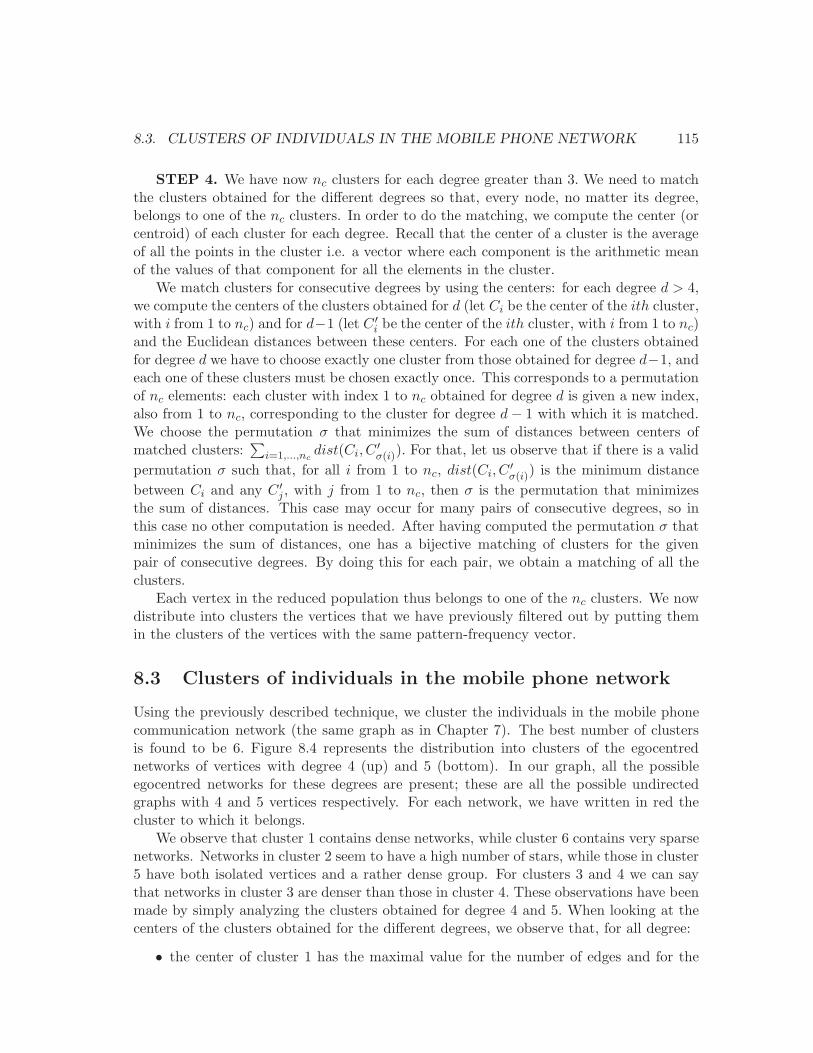
8.3. CLUSTERS OF INDIVIDUALS IN THE MOBILE PHONE NETWORK 115
STEP 4. We have now nc clusters for each degree greater than 3. We need to matchthe clusters obtained for the different degrees so that, every node, no matter its degree,belongs to one of the nc clusters. In order to do the matching, we compute the center (orcentroid) of each cluster for each degree. Recall that the center of a cluster is the averageof all the points in the cluster i.e. a vector where each component is the arithmetic meanof the values of that component for all the elements in the cluster.
We match clusters for consecutive degrees by using the centers: for each degree d > 4,we compute the centers of the clusters obtained for d (let Ci be the center of the ith cluster,with i from 1 to nc) and for d−1 (let C ′
i be the center of the ith cluster, with i from 1 to nc)and the Euclidean distances between these centers. For each one of the clusters obtainedfor degree d we have to choose exactly one cluster from those obtained for degree d−1, andeach one of these clusters must be chosen exactly once. This corresponds to a permutationof nc elements: each cluster with index 1 to nc obtained for degree d is given a new index,also from 1 to nc, corresponding to the cluster for degree d− 1 with which it is matched.We choose the permutation σ that minimizes the sum of distances between centers ofmatched clusters:
∑
i=1,...,ncdist(Ci, C
′σ(i)). For that, let us observe that if there is a valid
permutation σ such that, for all i from 1 to nc, dist(Ci, C′σ(i)) is the minimum distance
between Ci and any C ′j , with j from 1 to nc, then σ is the permutation that minimizes
the sum of distances. This case may occur for many pairs of consecutive degrees, so inthis case no other computation is needed. After having computed the permutation σ thatminimizes the sum of distances, one has a bijective matching of clusters for the givenpair of consecutive degrees. By doing this for each pair, we obtain a matching of all theclusters.
Each vertex in the reduced population thus belongs to one of the nc clusters. We nowdistribute into clusters the vertices that we have previously filtered out by putting themin the clusters of the vertices with the same pattern-frequency vector.
8.3 Clusters of individuals in the mobile phone network
Using the previously described technique, we cluster the individuals in the mobile phonecommunication network (the same graph as in Chapter 7). The best number of clustersis found to be 6. Figure 8.4 represents the distribution into clusters of the egocentrednetworks of vertices with degree 4 (up) and 5 (bottom). In our graph, all the possibleegocentred networks for these degrees are present; these are all the possible undirectedgraphs with 4 and 5 vertices respectively. For each network, we have written in red thecluster to which it belongs.
We observe that cluster 1 contains dense networks, while cluster 6 contains very sparsenetworks. Networks in cluster 2 seem to have a high number of stars, while those in cluster5 have both isolated vertices and a rather dense group. For clusters 3 and 4 we can saythat networks in cluster 3 are denser than those in cluster 4. These observations have beenmade by simply analyzing the clusters obtained for degree 4 and 5. When looking at thecenters of the clusters obtained for the different degrees, we observe that, for all degree:
• the center of cluster 1 has the maximal value for the number of edges and for the
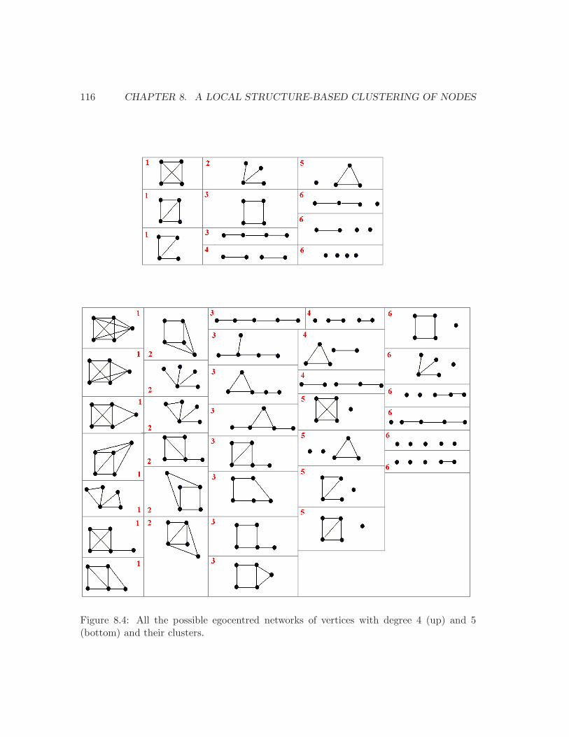
116 CHAPTER 8. A LOCAL STRUCTURE-BASED CLUSTERING OF NODES
Figure 8.4: All the possible egocentred networks of vertices with degree 4 (up) and 5(bottom) and their clusters.
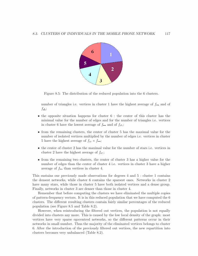
8.3. CLUSTERS OF INDIVIDUALS IN THE MOBILE PHONE NETWORK 117
Figure 8.5: The distribution of the reduced population into the 6 clusters.
number of triangles i.e. vertices in cluster 1 have the highest average of f and off ;
• the opposite situation happens for cluster 6 : the center of this cluster has theminimal value for the number of edges and for the number of triangles i.e. verticesin cluster 6 have the lowest average of f and of f ;
• from the remaining clusters, the center of cluster 5 has the maximal value for thenumber of isolated vertices multiplied by the number of edges i.e. vertices in cluster5 have the highest average of fiv × f ;
• the center of cluster 2 has the maximal value for the number of stars i.e. vertices incluster 2 have the highest average of f ;
• from the remaining two clusters, the center of cluster 3 has a higher value for thenumber of edges than the center of cluster 4 i.e. vertices in cluster 3 have a higheraverage of f than vertices in cluster 4.
This sustains our previously made observations for degrees 4 and 5 : cluster 1 containsthe densest networks, while cluster 6 contains the sparsest ones. Networks in cluster 2have many stars, while those in cluster 5 have both isolated vertices and a dense group.Finally, networks in cluster 3 are denser than those in cluster 4.
Remember that before computing the clusters we have eliminated the multiple copiesof pattern-frequency vectors. It is in this reduced population that we have computed the 6clusters. The different resulting clusters contain fairly similar percentages of the reducedpopulation (see Figure 8.5 and Table 8.2).
However, when reintroducing the filtered out vertices, the population is not equallydivided into clusters any more. This is caused by the low local density of the graph: mostvertices have very sparse egocentred networks, so the different patterns occur in theirnetworks in small number. Thus the majority of the eliminated vertices belongs to cluster6. After the introduction of the previously filtered out vertices, the new repartition intoclusters becomes very unbalanced (Table 8.2).
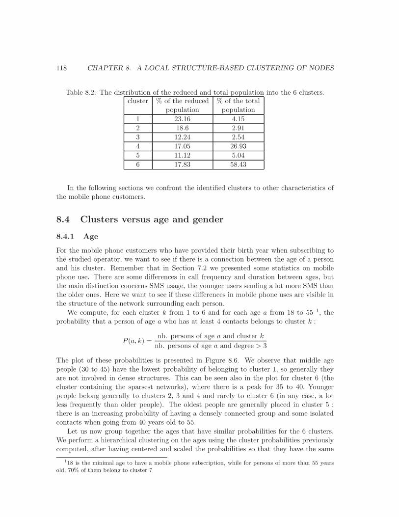
118 CHAPTER 8. A LOCAL STRUCTURE-BASED CLUSTERING OF NODES
Table 8.2: The distribution of the reduced and total population into the 6 clusters.cluster % of the reduced % of the total
population population
1 23.16 4.15
2 18.6 2.91
3 12.24 2.54
4 17.05 26.93
5 11.12 5.04
6 17.83 58.43
In the following sections we confront the identified clusters to other characteristics ofthe mobile phone customers.
8.4 Clusters versus age and gender
8.4.1 Age
For the mobile phone customers who have provided their birth year when subscribing tothe studied operator, we want to see if there is a connection between the age of a personand his cluster. Remember that in Section 7.2 we presented some statistics on mobilephone use. There are some differences in call frequency and duration between ages, butthe main distinction concerns SMS usage, the younger users sending a lot more SMS thanthe older ones. Here we want to see if these differences in mobile phone uses are visible inthe structure of the network surrounding each person.
We compute, for each cluster k from 1 to 6 and for each age a from 18 to 55 1, theprobability that a person of age a who has at least 4 contacts belongs to cluster k :
P (a, k) =nb. persons of age a and cluster k
nb. persons of age a and degree > 3
The plot of these probabilities is presented in Figure 8.6. We observe that middle agepeople (30 to 45) have the lowest probability of belonging to cluster 1, so generally theyare not involved in dense structures. This can be seen also in the plot for cluster 6 (thecluster containing the sparsest networks), where there is a peak for 35 to 40. Youngerpeople belong generally to clusters 2, 3 and 4 and rarely to cluster 6 (in any case, a lotless frequently than older people). The oldest people are generally placed in cluster 5 :there is an increasing probability of having a densely connected group and some isolatedcontacts when going from 40 years old to 55.
Let us now group together the ages that have similar probabilities for the 6 clusters.We perform a hierarchical clustering on the ages using the cluster probabilities previouslycomputed, after having centered and scaled the probabilities so that they have the same
118 is the minimal age to have a mobile phone subscription, while for persons of more than 55 yearsold, 70% of them belong to cluster 7
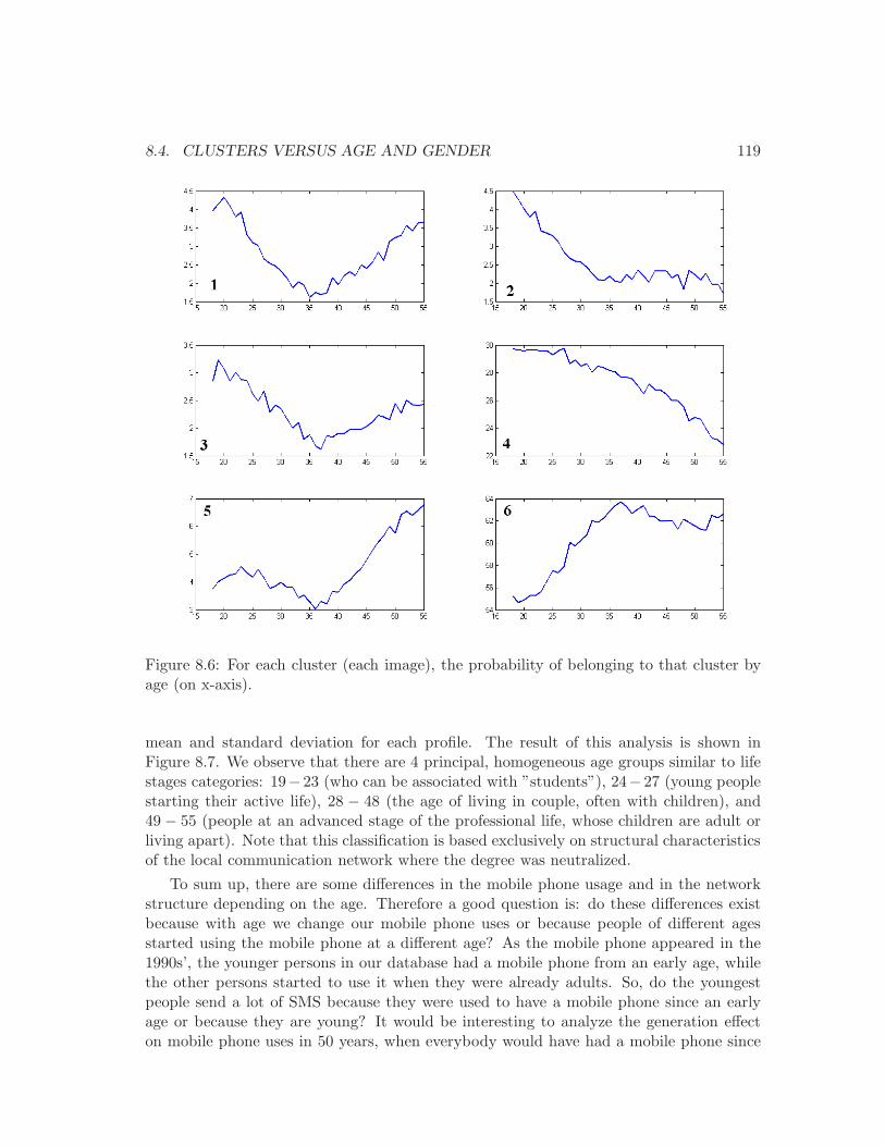
8.4. CLUSTERS VERSUS AGE AND GENDER 119
Figure 8.6: For each cluster (each image), the probability of belonging to that cluster byage (on x-axis).
mean and standard deviation for each profile. The result of this analysis is shown inFigure 8.7. We observe that there are 4 principal, homogeneous age groups similar to lifestages categories: 19− 23 (who can be associated with ”students”), 24− 27 (young peoplestarting their active life), 28 − 48 (the age of living in couple, often with children), and49 − 55 (people at an advanced stage of the professional life, whose children are adult orliving apart). Note that this classification is based exclusively on structural characteristicsof the local communication network where the degree was neutralized.
To sum up, there are some differences in the mobile phone usage and in the networkstructure depending on the age. Therefore a good question is: do these differences existbecause with age we change our mobile phone uses or because people of different agesstarted using the mobile phone at a different age? As the mobile phone appeared in the1990s’, the younger persons in our database had a mobile phone from an early age, whilethe other persons started to use it when they were already adults. So, do the youngestpeople send a lot of SMS because they were used to have a mobile phone since an earlyage or because they are young? It would be interesting to analyze the generation effecton mobile phone uses in 50 years, when everybody would have had a mobile phone since
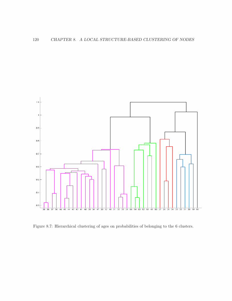
120 CHAPTER 8. A LOCAL STRUCTURE-BASED CLUSTERING OF NODES
Figure 8.7: Hierarchical clustering of ages on probabilities of belonging to the 6 clusters.
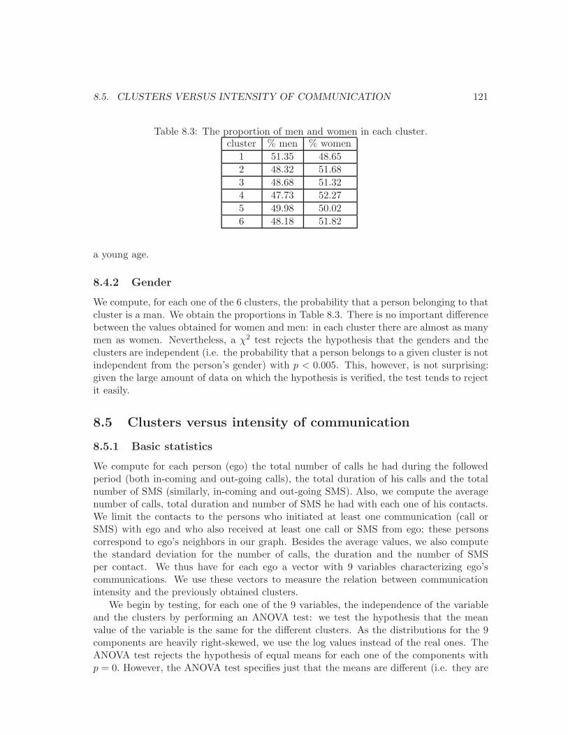
8.5. CLUSTERS VERSUS INTENSITY OF COMMUNICATION 121
Table 8.3: The proportion of men and women in each cluster.cluster % men % women
1 51.35 48.65
2 48.32 51.68
3 48.68 51.32
4 47.73 52.27
5 49.98 50.02
6 48.18 51.82
a young age.
8.4.2 Gender
We compute, for each one of the 6 clusters, the probability that a person belonging to thatcluster is a man. We obtain the proportions in Table 8.3. There is no important differencebetween the values obtained for women and men: in each cluster there are almost as manymen as women. Nevertheless, a χ2 test rejects the hypothesis that the genders and theclusters are independent (i.e. the probability that a person belongs to a given cluster is notindependent from the person’s gender) with p < 0.005. This, however, is not surprising:given the large amount of data on which the hypothesis is verified, the test tends to rejectit easily.
8.5 Clusters versus intensity of communication
8.5.1 Basic statistics
We compute for each person (ego) the total number of calls he had during the followedperiod (both in-coming and out-going calls), the total duration of his calls and the totalnumber of SMS (similarly, in-coming and out-going SMS). Also, we compute the averagenumber of calls, total duration and number of SMS he had with each one of his contacts.We limit the contacts to the persons who initiated at least one communication (call orSMS) with ego and who also received at least one call or SMS from ego; these personscorrespond to ego’s neighbors in our graph. Besides the average values, we also computethe standard deviation for the number of calls, the duration and the number of SMSper contact. We thus have for each ego a vector with 9 variables characterizing ego’scommunications. We use these vectors to measure the relation between communicationintensity and the previously obtained clusters.
We begin by testing, for each one of the 9 variables, the independence of the variableand the clusters by performing an ANOVA test: we test the hypothesis that the meanvalue of the variable is the same for the different clusters. As the distributions for the 9components are heavily right-skewed, we use the log values instead of the real ones. TheANOVA test rejects the hypothesis of equal means for each one of the components withp = 0. However, the ANOVA test specifies just that the means are different (i.e. they are
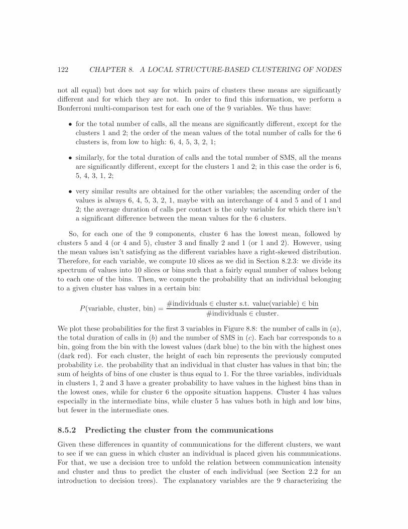
122 CHAPTER 8. A LOCAL STRUCTURE-BASED CLUSTERING OF NODES
not all equal) but does not say for which pairs of clusters these means are significantlydifferent and for which they are not. In order to find this information, we perform aBonferroni multi-comparison test for each one of the 9 variables. We thus have:
• for the total number of calls, all the means are significantly different, except for theclusters 1 and 2; the order of the mean values of the total number of calls for the 6clusters is, from low to high: 6, 4, 5, 3, 2, 1;
• similarly, for the total duration of calls and the total number of SMS, all the meansare significantly different, except for the clusters 1 and 2; in this case the order is 6,5, 4, 3, 1, 2;
• very similar results are obtained for the other variables; the ascending order of thevalues is always 6, 4, 5, 3, 2, 1, maybe with an interchange of 4 and 5 and of 1 and2; the average duration of calls per contact is the only variable for which there isn’ta significant difference between the mean values for the 6 clusters.
So, for each one of the 9 components, cluster 6 has the lowest mean, followed byclusters 5 and 4 (or 4 and 5), cluster 3 and finally 2 and 1 (or 1 and 2). However, usingthe mean values isn’t satisfying as the different variables have a right-skewed distribution.Therefore, for each variable, we compute 10 slices as we did in Section 8.2.3: we divide itsspectrum of values into 10 slices or bins such that a fairly equal number of values belongto each one of the bins. Then, we compute the probability that an individual belongingto a given cluster has values in a certain bin:
P (variable, cluster, bin) =#individuals ∈ cluster s.t. value(variable) ∈ bin
#individuals ∈ cluster.
We plot these probabilities for the first 3 variables in Figure 8.8: the number of calls in (a),the total duration of calls in (b) and the number of SMS in (c). Each bar corresponds to abin, going from the bin with the lowest values (dark blue) to the bin with the highest ones(dark red). For each cluster, the height of each bin represents the previously computedprobability i.e. the probability that an individual in that cluster has values in that bin; thesum of heights of bins of one cluster is thus equal to 1. For the three variables, individualsin clusters 1, 2 and 3 have a greater probability to have values in the highest bins than inthe lowest ones, while for cluster 6 the opposite situation happens. Cluster 4 has valuesespecially in the intermediate bins, while cluster 5 has values both in high and low bins,but fewer in the intermediate ones.
8.5.2 Predicting the cluster from the communications
Given these differences in quantity of communications for the different clusters, we wantto see if we can guess in which cluster an individual is placed given his communications.For that, we use a decision tree to unfold the relation between communication intensityand cluster and thus to predict the cluster of each individual (see Section 2.2 for anintroduction to decision trees). The explanatory variables are the 9 characterizing the
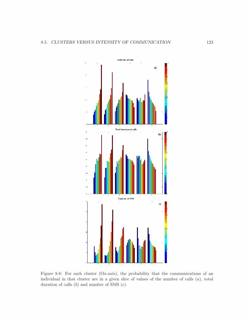
8.5. CLUSTERS VERSUS INTENSITY OF COMMUNICATION 123
Figure 8.8: For each cluster (Ox-axis), the probability that the communications of anindividual in that cluster are in a given slice of values of the number of calls (a), totalduration of calls (b) and number of SMS (c).
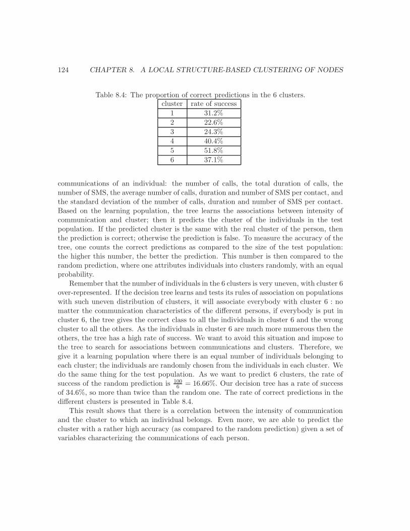
124 CHAPTER 8. A LOCAL STRUCTURE-BASED CLUSTERING OF NODES
Table 8.4: The proportion of correct predictions in the 6 clusters.cluster rate of success
1 31.2%
2 22.6%
3 24.3%
4 40.4%
5 51.8%
6 37.1%
communications of an individual: the number of calls, the total duration of calls, thenumber of SMS, the average number of calls, duration and number of SMS per contact, andthe standard deviation of the number of calls, duration and number of SMS per contact.Based on the learning population, the tree learns the associations between intensity ofcommunication and cluster; then it predicts the cluster of the individuals in the testpopulation. If the predicted cluster is the same with the real cluster of the person, thenthe prediction is correct; otherwise the prediction is false. To measure the accuracy of thetree, one counts the correct predictions as compared to the size of the test population:the higher this number, the better the prediction. This number is then compared to therandom prediction, where one attributes individuals into clusters randomly, with an equalprobability.
Remember that the number of individuals in the 6 clusters is very uneven, with cluster 6over-represented. If the decision tree learns and tests its rules of association on populationswith such uneven distribution of clusters, it will associate everybody with cluster 6 : nomatter the communication characteristics of the different persons, if everybody is put incluster 6, the tree gives the correct class to all the individuals in cluster 6 and the wrongcluster to all the others. As the individuals in cluster 6 are much more numerous then theothers, the tree has a high rate of success. We want to avoid this situation and impose tothe tree to search for associations between communications and clusters. Therefore, wegive it a learning population where there is an equal number of individuals belonging toeach cluster; the individuals are randomly chosen from the individuals in each cluster. Wedo the same thing for the test population. As we want to predict 6 clusters, the rate ofsuccess of the random prediction is 100
6 = 16.66%. Our decision tree has a rate of successof 34.6%, so more than twice than the random one. The rate of correct predictions in thedifferent clusters is presented in Table 8.4.
This result shows that there is a correlation between the intensity of communicationand the cluster to which an individual belongs. Even more, we are able to predict thecluster with a rather high accuracy (as compared to the random prediction) given a set ofvariables characterizing the communications of each person.
8.6. A TYPOLOGY OF CUSTOMERS 125
8.6 A typology of customers
In the previous two sections we compared the social network clusters first to customers’age and gender, and then to their communication intensity. We thus saw that the prob-ability that an individual belongs to a given cluster is not independent from his age orcommunication intensity.
Here we want to take into consideration, in the same time, all the 3 dimensions char-acterizing the individuals: the age, the communication intensity and the social networkcluster2. We want to see how these characteristics are distributed in the population andalso to create a typology of customers based on these 3 dimensions. We would thus obtaingroups of individuals such that the persons in a same group have similar communicationpractices and about the same age and cluster.
We use the Kohonen self organizing map in the same way as in Chapter 6. Rememberthat this clustering method produces a map with several layers, one for each variablecharacterizing the individuals. This shows how the different variables are distributedin the population. Also, the algorithm produces cells grouping individuals with closecharacteristics. In a second step, the algorithm computes a clustering of the individuals.The obtained clustering will represent our typology.
We choose the following parameters to characterize the individuals:
• age; this is the socio-demographic variable;
• cluster (from 1 to 6, as obtained in the previous sections); as it takes only 6 values,this variable can be seen as a class or a label of each individual; this is the socialnetwork variable;
• communication intensity: number of calls, total duration of calls and number ofSMS; these are the communication variables.
Each individual is thus characterized by a vector with 5 elements. For the commu-nication variables, we use a log transformation instead of the values themselves as thesevariables are heavily right-skewed. Also, recall that the distribution of individuals intoclusters is very uneven, with cluster 6 being overrepresented. As we want to measure theinfluence of the variable ”cluster”, too, we randomly choose a same number of individualsin each cluster.
The set of individuals is then processed by the Kohonen self organizing map. Thisalgorithm does not take labels into consideration when building the map, so it builds themap using only the other variables. However, in the graphic representation of the map,it draws a layer for the labels, too. On this layer the different cells are colored dependingon the labels of the individuals in the cells: the color of the cell corresponds to the labelthat occurs the most for the individuals in that cell.
The processing of the set of individuals by the SOM provides Figure 8.9. We observethat, unsurprisingly, the number of calls and the total duration are highly correlated, with
2We do not take into consideration the gender because its influence on the cluster is not very strong;besides, this variable takes only 2 values
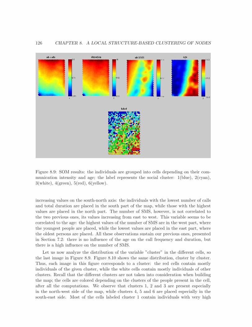
126 CHAPTER 8. A LOCAL STRUCTURE-BASED CLUSTERING OF NODES
Figure 8.9: SOM results: the individuals are grouped into cells depending on their com-munication intensity and age; the label represents the social cluster: 1(blue), 2(cyan),3(white), 4(green), 5(red), 6(yellow).
increasing values on the south-north axis: the individuals with the lowest number of callsand total duration are placed in the south part of the map, while those with the highestvalues are placed in the north part. The number of SMS, however, is not correlated tothe two previous ones, its values increasing from east to west. This variable seems to becorrelated to the age: the highest values of the number of SMS are in the west part, wherethe youngest people are placed, while the lowest values are placed in the east part, wherethe oldest persons are placed. All these observations sustain our previous ones, presentedin Section 7.2: there is no influence of the age on the call frequency and duration, butthere is a high influence on the number of SMS.
Let us now analyze the distribution of the variable ”cluster” in the different cells, sothe last image in Figure 8.9. Figure 8.10 shows the same distribution, cluster by cluster.Thus, each image in this figure corresponds to a cluster: the red cells contain mostlyindividuals of the given cluster, while the white cells contain mostly individuals of otherclusters. Recall that the different clusters are not taken into consideration when buildingthe map; the cells are colored depending on the clusters of the people present in the cell,after all the computations. We observe that clusters 1, 2 and 3 are present especiallyin the north-west side of the map, while clusters 4, 5 and 6 are placed especially in thesouth-east side. Most of the cells labeled cluster 1 contain individuals with very high
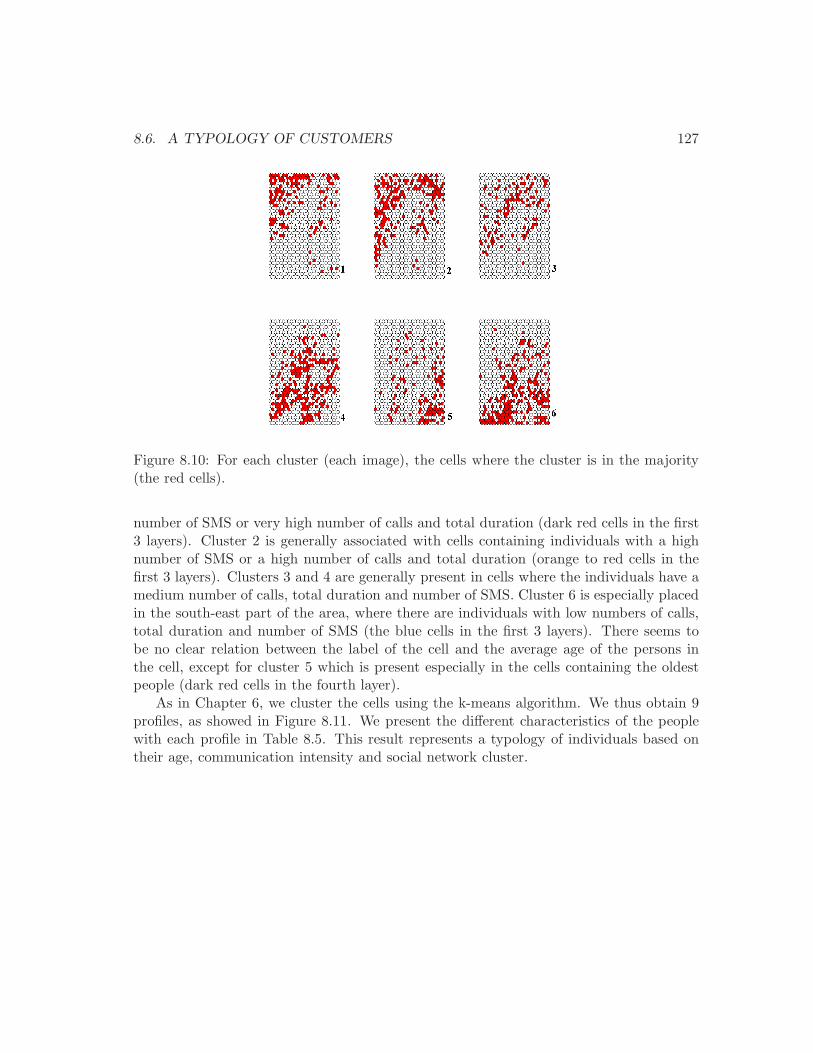
8.6. A TYPOLOGY OF CUSTOMERS 127
Figure 8.10: For each cluster (each image), the cells where the cluster is in the majority(the red cells).
number of SMS or very high number of calls and total duration (dark red cells in the first3 layers). Cluster 2 is generally associated with cells containing individuals with a highnumber of SMS or a high number of calls and total duration (orange to red cells in thefirst 3 layers). Clusters 3 and 4 are generally present in cells where the individuals have amedium number of calls, total duration and number of SMS. Cluster 6 is especially placedin the south-east part of the area, where there are individuals with low numbers of calls,total duration and number of SMS (the blue cells in the first 3 layers). There seems tobe no clear relation between the label of the cell and the average age of the persons inthe cell, except for cluster 5 which is present especially in the cells containing the oldestpeople (dark red cells in the fourth layer).
As in Chapter 6, we cluster the cells using the k-means algorithm. We thus obtain 9profiles, as showed in Figure 8.11. We present the different characteristics of the peoplewith each profile in Table 8.5. This result represents a typology of individuals based ontheir age, communication intensity and social network cluster.
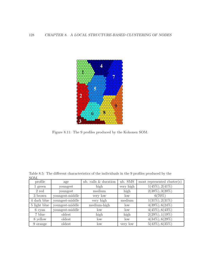
128 CHAPTER 8. A LOCAL STRUCTURE-BASED CLUSTERING OF NODES
Figure 8.11: The 9 profiles produced by the Kohonen SOM.
Table 8.5: The different characteristics of the individuals in the 9 profiles produced by theSOM.
profile age nb. calls & duration nb. SMS most represented cluster(s)
1 green youngest high very high 1(45%), 2(41%)
2 red youngest medium high 2(38%), 3(20%)
3 brown youngest-middle very low low 6(70%)
4 dark blue youngest-middle very high medium 1(31%), 2(31%)
5 light blue youngest-middle medium-high low 4(39%), 6(24%)
6 cyan youngest-middle low low 4(45%), 6(43%)
7 blue oldest high high 2(29%), 1(19%)
8 yellow oldest low low 4(34%), 6(29%)
9 orange oldest low very low 5(42%), 6(35%)
8.7. CHAPTER CONCLUSIONS 129
8.7 Chapter conclusions
In this chapter we continued the analysis of the mobile phone graph with a clustering ofnodes, thus relating to the problem of identification of roles in a network. In this problemoften encountered in social network analysis, one wants to group together the nodes ofthe network that are connected in similar ways to the network. There are however severalquestions that make this problem difficult to solve: What is a good characterization of theway a node is connected to the network? What does ”similar connections” mean? Canthe solution be applied to large graphs? How can one check the relevance of the differentgroups of nodes? In which conditions can one say that there is no better way of groupingthe nodes?
We have made several choices in order to answer the different questions. First, wehave characterized the way a node is connected to the network by counting the patternspresent in its egocentred network; we have stored the number of occurrences of the differentpatterns in a pattern-frequency vector characterizing the node. Second, we have consideredthat nodes connected in a similar way to the network have close pattern-frequency vectors;here ”close” is defined with respect to a set of transformations made on the pattern-frequency vectors. We have thus proposed a method for nodes clustering that groupstogether vertices that are embedded in similar egocentred networks. The clustering isdone efficiently, so the method can be applied to large graphs. As said before, we havemade several choices in order to answer the different questions. The proposed methodgives promising results when applied to our real-world graph. As always, in this kind ofmethods, the solution validation is a delicate problem, but the results we have obtainedfor our large social network sustain the relevance of our method.
We have applied the proposed method to the mobile phone graph described in theprevious chapter. This graph models one-month mobile phone communications betweenthe 3 million customers of Mobistar. The clusters produced by the method can be seen asa segmentation of the set of customers based on their social network insertions. We havecompared the different clusters to the other information we had on the individuals (age,gender and communication intensity), showing that the different parameters characterizingthe individuals are not independent. Thus, the probability that a node belongs to agiven cluster is not independent from the age, gender or mobile phone use of the personrepresented by the node. These results confirm the soundness of our method, even though,as always, many concurrent clusterings for various purposes may as well be relevant.

130 CHAPTER 8. A LOCAL STRUCTURE-BASED CLUSTERING OF NODES

Part III
Conclusions
131

133
The main goal of our research was to characterize the individuals connected in asocial network by analyzing the local structure of the network. For that, we proposed amethod that describes the way a node (corresponding to an individual) is embedded inthe network. This method provides a characterization of the individual and also of therelative positions occupied by the neighbors of the node in its egocentred network (whichcan also be seen as a description of how the links formed by a node are embedded in thenetwork). Our method is related to the analysis of egocentred networks in sociology andto the local approach in the study of complex networks. As it takes into consideration onlythe surrounding network when analyzing one node, it can be applied to small networks,to fractions of networks (one does not need the entire network when analyzing one node)and also to large networks; this is due to its rather small complexity, depending only onthe number of neighbors of the node. Although in this thesis we applied the method onlyto social networks, it can be applied in the same way to any other graph, no matter itsorigin.
We applied the method we introduced to two large social networks, one modelingonline activity on MySpace (a platform for social networking and video publishing), theother one modeling mobile phone communications. In the first case we were interested inanalyzing the online popularity of artists on MySpace. We first grouped individuals intoclusters using their popularity characteristics (mainly their online audience and authority),thus obtaining 5 clusters. Besides two unsurprising categories (very popular artists andunknown artists), we identified two different clusters of medium popularity and a categoryof small but socially active artists. Next we compared the obtained clusters to the localstructure of the network surrounding each node, so we analyzed the popularity of artistsin relation with the structure of the network in which they are embedded. We thusshowed that artists in different categories exhibit different insertions in the social network.On the one hand, artists with a low authority and non reciprocal links tend to declarevery popular artists as best friends thus generating a star structure. On the other hand,some medium and low popularity artists with many reciprocal links form cliques with theirneighbors, thus creating dense communities, without stars but with triangles. Our researchon MySpace belongs to the analysis of popularity on online networks, where researcherstry to discover how fame is built, what strategies users employ, how they adapt theirpublishing and networking practices in order to be popular. There are many studies onthis competition for online popularity, but they focus either on published content andits popularity, either on the structure of the social network embedding the users. Herewe tried to hold together the two approaches, so to make the connection between fameand social linkage. The same kind of analysis, using the methods we employed here,can be done on other online platforms where the popularity can be measured and thesocial network can be built. An immediate transposition can be imagined for Flickr andYoutube for instance. In the same way, one can also study offline networks for which thereare recordings of users’ activity, as for instance a mobile phone communications network.It is such a network that we analyzed next, but in a different approach.
We used the list of one-month communications between 3 million mobile phone users.We were interested in three aspects that we tried to compare: social-demographic data(users’ age and gender), communication intensity (for each couple of persons, their num-
134
ber of calls, duration of calls and number of SMS) and social network structure. Firstwe confirmed, using these large amounts of data, some existing sociological theories oncommunication duration depending on receiver’s gender and on young people’s tendencyto send SMS. Next, by applying the method introduced previously, we analyzed the localstructure of the social network modeling the set of mobile phone communications. Theresults of our method gave us the possibility to test several definitions of characteristicpatterns, thus relating to two popular problems in data mining and bioinformatics: thefrequent patterns discovery and the network motifs identification. Next, we analyzed thepositions occupied by the neighbors of each node (ego) and we compared them to thequantity of communication with ego. We thus saw that the person that speaks the mostwith ego has an important position in his egocentred network. If this result seams in-tuitive, it isn’t necessarily straightforward if there is the person who speaks the most asnumber of calls or the one who speaks the most as total duration of calls who has themost important position. In our dataset, it is the person with the highest frequency ofcalls who has a more important place in the egocentred network; this result is sustainedby an existing sociological study on patterns of communication.
In our opinion, the next logical step of our analysis was to group together nodes withsimilar egocentred networks, so connected in the same way to the network. This is theproblem of identification of roles in a network. Without pretending to have solved thisproblem, we proposed a method for grouping the nodes of a large network that we appliedto the mobile phone social network. One of the main problems when trying to identifythe roles played by the different nodes of the network is the results validation. In smallnetworks one can simply look at the different nodes and decide if the attributed rolescorrespond to the structure of the network surrounding each node. Of course one cannotdo this in large networks. This is why we cannot pretend having solved the problem ofidentifying social roles. We simply proposed a way to cluster nodes depending on the localstructure of the network; there may be other clusterings with more satisfying attributionsof roles of nodes. However, the results obtained when applying the method to the mobilephone social network are quite promising. We compared the 6 clusters of mobile phoneusers identified by the method to the two other dimensions characterizing the individuals:the socio-demographic data and the intensity of communication. A first observation is thatbelonging to a certain cluster is not independent from users’ age, gender and intensity ofcommunication. Even more, by using the distribution of persons of different ages intoclusters, we were able to identify 4 homogeneous age groups, corresponding to life stages.And this using only the way the nodes are connected to the network, independently fromthe number of neighbors of each node. Next, we were able to predict with a rather highprobability the cluster of each person using his communication intensity, thus showingthat local structure and communication intensity are correlated. Persons embedded indense structures seem to communicate more by mobile phone than persons belongingto sparse networks. These results make us believe in the relevance of our method fornodes clustering. This method can be easily applied to any large network; it will clusternodes depending on the structure of the network surrounding them. It is important toprecise that our method groups together nodes that are connected in the same way whencomparing to the other nodes of the network and not to a theoretical situation or to nodes
135
of other networks. Thus a node belongs to a certain cluster because it is similar to theother nodes of the cluster and different from the other nodes of the network, of this precisenetwork. The clustering of nodes depends entirely on the structure of the given network,as it is in this network that we want to find groups of nodes.
These are the main conclusions of our work during this thesis. A lot of extensions andimprovements can be imagined; we present some of them in the following section.
Further work
As said before, the set of methods we used here can be easily applied to other (social)networks. Using the local structures in which nodes are embedded, it would be interestingfor instance to compute clusters of individuals in social networks that are denser thanthe mobile phone one but sparser than the MySpace one. In the mobile phone network,many links are missing: maybe two persons contact each other by different means, butnot by mobile phone. Thus, in our graph, we see the two persons as not connected and weanalyze them in consequence, although they do connect, but by means that are not visibleto us. On the contrary, in social networks modeling online activities, there are many linksthat do not correspond to a real, social relation between the two persons. As we saw inthe study on MySpace popularity, people connect to other people they do not know, justbecause they are popular, creating thus a fan-star structure. Such social networks aretherefore denser than the ”real” social network where each link corresponds to a socialrelation between the two persons. For the mobile phone graph, we search for clusters ofindividuals in a network that is sparser than the real one, while for the online networks,we search in a graph that is denser than the real network. It would be thus interesting toanalyze a graph with a density between the two.
In another perspective, the method itself could be improved. For instance one couldcharacterize the way each node is connected to the network by analyzing the network atat most 2 (or more) steps from the node i.e. the network formed by ego’s neighbors, theirneighbors and the links between all these nodes. However, the computation and resultscomplexity might increase a lot. Also one would have to deal with the distinction betweendirect neighbors and distance−2 neighbors. Maybe an easier way to take into considerationthe distance−2 neighborhood is to analyze in more details how different individuals (withdifferent local characteristics) connect to each other. One can see the global network asthe union of many egocentred networks that partially overlap. It would be interesting tosee how and why they overlap, for which type of egocentred network, in which proportionetc.
Another improvement can be done by taking into consideration the weight of linkswhen computing patterns. For instance, for the mobile phone social network, one canput a weight on the links using the frequency of calls and their duration or the frequencyof SMS. Then, instead of characterizing a node by the number of patterns present in itsegocentred network, one could characterize it using the number of weighted patterns. Theweight of the pattern can be for instance the following couple: average weight of links inthe pattern, standard deviation of weight of links in the pattern. One has thus an idea of
136
the quantity of information that flows in the pattern and also of its distribution (balancedof not). Characterizing nodes by counting weighted patterns would offer a more detaileddescription of how each node is connected to the network.
Also one could give a weight or simply a color to the nodes of the network (insteadof the links). This can be done at the global level, by coloring each node of the networkdepending on some statistics, at the local level, by coloring each node in the egocentrednetwork depending on its relation with ego, or at the intermediate level, for instance bycoloring the nodes depending on the community they belong to. Then, instead of simplycounting patterns, one could count patterns with different combinations of colors on theirnodes. Maybe such an approach would provide a better definition of characteristic patters.
Another possible direction is to take into consideration the temporal dynamics of thenetwork. For instance one could try to predict the cluster to which a node will belongin a second network (obtained some time after the first network) by using the cluster ofthe node (and maybe other characteristics) in the first network. Or one could predictsome events (like the formation or the deletion of links) by using the way the nodes areembedded into the network. Maybe the fact of having many stars or triangles etc. in theegocentred network says something about the capacity of a node of adding new links or ofloosing existing ones. One could also describe how the different nodes evolve in time bycomputing their cluster in different snapshots of the same network. From this descriptionone could compute patterns of evolution or see if the way of changing the cluster is relatedto other information on the nodes. For instance in the mobile phone social network onecan see if the individuals remain in the same cluster from one period to the other, ifthey change, how they change and how their evolution is related to their age or gender.In an even more precise approach one could analyze the local structure of the networkdynamically i.e. when each event happens (as for instance the formation or deletion oflinks).

Bibliography
[AA04] Istvan Albert and Reka Albert. Conserved network motifs allow protein-protein interaction prediction. Bioinformatics, 20(18):3346–3352, 2004.
[ABA03] Lada A. Adamic, Orkut Buyukkokten, and Eytan Adar. A social networkcaught in the web. First Monday, 8(6), 2003.
[AD07] B. Bassett et J. Hoskins Allsop D. Word-of-mouth research: principles andapplications. Journal of Advertising Research, 34:398–411, 2007.
[AGMN92] Noga Alon, Zvi Galil, Oded Margalit, and Moni Naor. Witnesses for booleanmatrix multiplication and for shortest paths. In FOCS, pages 417–426.IEEE, 1992.
[AH01] Lada A. Adamic and Bernardo A. Huberman. The web’s hidden order.Communications of the ACM, 44(9):55–60, September 2001.
[AJB99] R. Albert, H. Jeong, and A. L. Barabasi. Diameter of the world-wide web.Nature (London), 401(6749):130, 1999.
[And06] D. Anderson. The Long Tail: How the Future of Business is Selling Less ofMore. Hyperion Books; New York edition, 2006.
[ARFBTS04] Y. Artzy-Randrup, S.J. Fleishman, N. Ben-Tal, and L. Stone. Commenton ”network motifs: Simple building blocks of complex networks” and ”su-perfamilies of evolved and designed networks”. Science, 305(5687):1107,August 2004.
[AS94] Rakesh Agrawal and Ramakrishnan Srikant. Fast algorithms for miningassociation rules in large databases. In VLDB, pages 487–499, 1994.
[ASBS00] L. A. N. Amaral, A. Scala, M. Barthelemy, and H. E. Stanley. Classes ofsmall-world networks. In Proceeding of the National Academy of Sciences,2000.
[ATSK04] M.J Aartsen, T.G. Van Tilburg, C.H.M Smits, and C.P.M. Knipscheer. Alongitudinal study on the impact of physical and cognitive decline on thepersonal network in old age. Journal of Social and Personal Relationships,21:249–266, 2004.
137
138 BIBLIOGRAPHY
[AYZ97] Noga Alon, Raphael Yuster, and Uri Zwick. Finding and counting givenlength cycles. Algorithmica, 17(3):209–223, 1997.
[AZBA08] Lada A. Adamic, Jun Zhang, Eytan Bakshy, and Mark S. Ackerman. Knowl-edge sharing and yahoo answers: everyone knows something. In WWW ’08:Proceeding of the 17th international conference on World Wide Web, pages665–674, New York, NY, USA, 2008. ACM.
[BA99] A.-L. Barabasi and R. Albert. Emergence of scaling in random networks.Science, 286(5439):509–512, 1999.
[Bar54] John A. Barnes. Class and committees in a Norwegian island parish. HumanRelations, 7:39–58, 1954.
[Bar02] Albert-Laszlo Barabasi. Linked: The New Science of Networks. PerseusBooks Group, 2002.
[BC09] J.S Beuscart and T. Couronne. The distribution of online reputation. InICWSM’09, May 2009.
[BCP02] K.K. Bost, M.J. Cox, and C. Payne. Structural and supportive changes incouples’ family and friendship networks across the transition to parenthood.Journal of Marriage and Family, 64:517–531, 2002.
[BDE09] Murat Ali Bayir, Murat Demirbas, and Nathan Eagle. Discovering spa-tiotemporal mobility profiles of cellphone users. In WOWMOM, pages 1–9.IEEE, 2009.
[BE89] S.P. Borgatti and M.G. Everett. The class of all regular equivalences: Al-gebraic structure and computation. Social Networks, 11(1):65–88, March1989.
[BGLL08] Vincent D Blondel, Jean-Loup Guillaume, Renaud Lambiotte, and EtienneLefebvre. Fast unfolding of communities in large networks. Journal ofStatistical Mechanics: Theory and Experiment, (10):P10008 (12pp), 2008.
[BHKL06] Lars Backstrom, Dan Huttenlocher, Jon Kleinberg, and Xiangyang Lan.Group formation in large social networks: membership, growth, and evolu-tion. In KDD ’06: Proceedings of the 12th ACM SIGKDD international con-ference on Knowledge discovery and data mining, pages 44–54, New York,NY, USA, 2006. ACM Press.
[BJN+02] A. L. Barabasi, H. Jeong, Z. Neda, E. Ravasz, A. Schubert, and T. Vic-sek. Evolution of the social network of scientific collaborations. Physica A:Statistical Mechanics and its Applications, 311(3-4):590 – 614, 2002.
[Boi74] J. Boissevain. Friends of Friends, Networks, Manipulators and Coalitions.Basil Blackwell, Oxford, 1974.
BIBLIOGRAPHY 139
[Bon87] Phillip Bonacich. Power and centrality: A family of measures. AmericanJournal of Sociology, 92(5):1170–1182, 1987.
[Bot57] Elizabeth Bott. Family and Social Network. Tavistock, London, 1957.
[BP98] Sergey Brin and Lawrence Page. The anatomy of a large-scale hypertextualWeb search engine. Computer Networks and ISDN Systems, 30(1–7):107–117, 1998.
[Bra01] Ulrik Brandes. A faster algorithm for betweenness centrality. Journal ofMathematical Sociology, 25(2):163–177, 2001.
[BT02] Tian Bu and Donald F. Towsley. On distinguishing between internet powerlaw topology generators. In INFOCOM, 2002.
[Bur92] R. Burt. Structural Holes. The Social Structure of Competition. Cambridge,Harvard University Press, 1992.
[Bur01] Ronald S. Burt. Structural holes versus network closure as social capital.In Nan Lin, Karen S. Cook, and Ronald S. Burt, editors, Social Capital:Theory and Research, pages 31–56. Aldine de Gruyter, New York, 2001.
[CF06] D. Chakrabarti and C. Faloutsos. Graph mining: Laws, generators, andalgorithms. ACM Computing Surveys (CSUR), 38(1), 2006.
[CG05] Dominique Cardon and Fabien Granjon. Social networks and cultural prac-tices a case study of young avid screen users in france. Social Networks,27:301–315, 2005.
[CKR+07] Meeyoung Cha, Haewoon Kwak, Pablo Rodriguez, Yong-Yeol Ahn, and SueMoon. I tube, you tube, everybody tubes: analyzing the world’s largest usergenerated content video system. In IMC’07, 2007.
[CLR01] T. H. Cormen, C. E. Leiserson, and T. L. Rivest. Introduction to Algorithms.The MIT Press, 2001.
[CM06] Judith A. Chevalier and Dina Mayzlin. The effect of word of mouth onsales: Online book reviews. Journal of Marketing Research, 43(3):345–354,August 2006.
[CMG09] Meeyoung Cha, Alan Mislove, and P. Krishna Gummadi. A measurement-driven analysis of information propagation in the flickr social network. InWWW, pages 721–730, 2009.
[CMN04] Aaron Clauset, Cristopher Moore, and M.E.J. Newman. Finding communitystructure in very large networks. Physical Review E, 70(6), 2004.
[Col88] J.S. Coleman. Social capital in the creation of human capital. Americanjournal of sociology, 94(S1):95, 1988.
140 BIBLIOGRAPHY
[CR04] Junghoo Cho and Sourashis Roy. Impact of search engines on page popu-larity. In Proceedings of the 13th conference on World Wide Web, 2004.
[CS08] Riley Crane and D. Sornette. Quality, and junk videos on youtube: Sepa-rating content from noise in an information-rich environment. In The 2008AAAI Spring Symposium, 2008.
[CSB10] T. Couronne, A. Stoica, and J.S. Beuscart. Online social network popularityevolution: an additive mixture model. In The 2010 International Conferenceon Advances in Social Networks Analysis and Mining (ASONAM), 2010.
[CSN07] Aaron Clauset, Cosma R. Shalizi, and M.E.J. Newman. Power-law distri-butions in empirical data. SIAM Reviews, June 2007.
[CW87] Don Coppersmith and Shmuel Winograd. Matrix multiplication via arith-metic progressions. In STOC, pages 1–6. ACM, 1987.
[DR01] P. Domingos and M. Richardson. Mining the network value of customers.In Proceedings of the Seventh ACM SIGKDD International Conference onKnowledge Discovery and Data Mining, 2001.
[DT99] Luc Dehaspe and Hannu Toivonen. Discovery of frequent DATALOG pat-terns. Data Mining and Knowledge Discovery, 3(1):7–36, 1999.
[DWM02] Jennifer A. Dunne, Richard J. Williams, and Neo D. Martinez. Food-webstructure and network theory: The role of connectance and size. PNAS,99(20):12917–12922, 2002.
[EB93] M.G. Everett and S.P. Borgatti. Two algorithms for computing regularequivalence. Social Networks, 15(4):361–376, 1993.
[EBK69] J. Engel, R. Blackwell, and R. Kegerreis. How information is used to adoptan innovation. Journal of Advertising Research, 9:3–8, 1969.
[EP05] Nathan Eagle and Alex Pentland. Social serendipity: Mobilizing socialsoftware. IEEE Pervasive Computing, 4(2):p28 – 34, 2005.
[ER60] Paul Erdos and Alfred Renyi. On the evolution of random graphs. Publi-cation of the Mathematical Institute of the Hungarian Academy of Science,pages 17–61, 1960.
[Eve80] Brian Everitt. Cluster Analysis. Halsted Press, London; New York, secondedition, 1980.
[EW04] David Eppstein and Joseph Wang. Fast approximation of centrality. Journalof Graph Algorithms Applications, 8(1):39–45, 2004.
BIBLIOGRAPHY 141
[FFF99] Michalis Faloutsos, Petros Faloutsos, and Christos Faloutsos. On power-law relationships of the internet topology. In SIGCOMM ’99: Proceedingsof the conference on Applications, technologies, architectures, and protocolsfor computer communication, New York, NY, USA, 1999.
[FLG00] Gary William Flake, Steve Lawrence, and C. Lee Giles. Efficient identifica-tion of web communities. In Sixth International Conference on KnowledgeDiscovery and Data Mining (ACM SIGKDD 2000), pages 150–160. ACM,2000.
[FM91] Toms Feder and Rajeev Motwani. Clique partitions, graph compression,and speeding-up algorithms. In STOC, pages 123–133. ACM, 1991.
[For10] Santo Fortunato. Community detection in graphs. Physics Reports, 486(3-5):75 – 174, 2010.
[FPSSU96] Usama M. Fayyad, Gregory Piatetsky-Shapiro, Padhraic Smyth, and Ra-masamy Uthurusamy. Advances in Knowledge Discovery and Data Mining.AAAI/MIT Press, 1996.
[Fra95] Robert H. Frank. The winner-take-all society. Free Press, New York, 1995.
[Fre77] Linton C. Freeman. A Set of Measures of Centrality Based on Betweenness.Sociometry, 40(1):35–41, 1977.
[FS65] S. Feldman and M. Spencer. The effect of personal influence in the selectionof consumer services. In Proceedings of the Fall Conference of the AmericanMarketing Association, 1965.
[FSW06] Danyel Fisher, Marc Smith, and Howard T. Welser. You are who you talkto: Detecting roles in usenet newsgroups. In Proceedings of the 39th HawaiiInternational Conference on System Sciences, 2006.
[Gal67] T. Gallai. Transitiv orientierbare graphen. Acta Mathematica Hungarica,18(1-2):25–66, 1967.
[GDS+03] Krishna P. Gummadi, Richard J. Dunn, Stefan Saroiu, Steven D. Gribble,Henry M. Levy, and John Zahorjan. Measurement, modeling, and analysisof a peer-to-peer file-sharing workload. In SOSP ’03: Proceedings of thenineteenth ACM symposium on Operating systems principles, pages 314–329, New York, NY, USA, 2003. ACM.
[GH06] Scott A. Golder and Bernardo A. Huberman. Usage patterns of collaborativetagging systems. Journal of Information Science, 32(2):198–208, 2006.
[GHB08] Marta C. Gonzalez, Cesar A. Hidalgo, and Albert-Laszlo Barabasi. Under-standing individual human mobility patterns. Nature, 453(7196):779–782,June 2008.
142 BIBLIOGRAPHY
[Gla00] Malcolm Gladwell. The tipping point: how little things can make a bigdifference. Little Brown, Boston, 1st edition, 2000.
[GN02] Michelle Girvan and M. E. J. Newman. Community structure in social andbiological networks. In Proceedings of the National Academy of Sciences,2002.
[GR03] D.S. Goldberg and F.P. Roth. Assessing experimentally derived interac-tions in a small world. Proceedings of the National Academy of Sciences,100(8):4372–4376, 2003.
[Gra78] M. Granovetter. The strength of weak ties. American Journal of Sociology,pages 1360–1380, 1978.
[Gri98] Maurizio Gribaudi. Espaces, temporalites, stratifications. Exercices sur lesreeseaux sociaux. EHESS, Paris, 1998.
[Gro05] Michel Grossetti. Where do social relations come from?: A study of personalnetworks in the Toulouse area of France. Social Networks, 27(4):289 – 300,2005.
[Hal08] A. Halavais. Do dugg diggers digg diligently. In AOIR’08, 2008.
[Hay05] Caroline Haythornthwaite. Social networks and internet connectivity effects.Information, Communication and Society, 8(2):125–147, June 2005.
[HBB07] T. Holloway, M. Bozicevic, and K. Borner. Analyzing and visualizing thesemantic coverage of wikipedia and its authors. Complexity, 12(3):30–40,2007.
[HCD94] Lawrence B. Holder, Diane J. Cook, and Surnjani Djoko. Substucture dis-covery in the subdue system. In KDD Workshop, pages 169–180, 1994.
[HEL04] Petter Holme, Christofer R. Edling, and Fredrik Liljeros. Structure andtime-evolution of an internet dating community. Social Networks, 26(2):155–174, 2004.
[HK79] Frank Harary and Helene J. Kommel. Matrix measures for transitivity andbalance. Journal of Mathematical Sociology, 6:199–210, 1979.
[HKP+05] Susan C. Herring, Inna Kouper, John C. Paolillo, Lois Ann Scheidt, MichaelTyworth, Peter Welsch, Elijah Wright, and Ning Yu. Conversations in theblogosphere: An analysis ”from the bottom up”. In HICSS’05, 2005.
[HM79] Michel Habib and M. C. Maurer. On the x-join decomposition for undirectedgraphs. Discrete Applied Mathematics, 3:198–207, 1979.
[HP57] Frank Harary and Herbert H. Paper. Toward a general calculus of phone-mic distribution. Language : Journal of the Linguistic Society of America,33:143–169, 1957.
BIBLIOGRAPHY 143
[HRS08] Cesar A. Hidalgo and C. Rodriguez-Sickert. The dynamics of a mobilephone network. Physica A: Statistical Mechanics and its Applications,387(12):3017–3024, May 2008.
[HRW08] Bernardo A. Huberman, Daniel M. Romero, and Fang Wu. Crowdsourcing,attention and productivity. CoRR, abs/0809.3030, 2008.
[HS] H. He and A.K. Singh. Graphrank: Statistical modeling and mining ofsignificant subgraphs in the feature space. In ICDM ’06.
[HTF01] T. Hastie, R. Tibshirani, and J. Friedman. The Elements of StatisticalLearning. Springer, 2001.
[ILK+05] Shalev Itzkovitz, Reuven Levitt, Nadav Kashtan, Ron Milo, MichaelItzkovitz, and Uri Alon. Coarse-graining and self-dissimilarity of com-plex networks. Physical Review E (Statistical, Nonlinear, and Soft MatterPhysics), 71(1), 2005.
[IR78] Alon Itai and Michael Rodeh. Finding a minimum circuit in a graph. SIAMJ. Comput., 7(4):413–423, 1978.
[IWM00] A. Inokuchi, T. Washio, and H. Motoda. An apriori-based algorithm formining frequent substructures from graph data. In Proceedings of the 4thEuropean Conference on Principles of Data Mining and Knowledge Discov-ery, pages 13–23, London, UK, 2000. Springer-Verlag.
[JBLE01] Jeffrey C. Johnson, Stephen P. Borgatti, Joseph J. Luczkovich, and Mar-tin G. Everett. Network role analysis in the study of food webs: An appli-cation of regular role coloration. Journal of Social Structure, 2(3), 2001.
[JMBO01] H. Jeong, S.P. Mason, A.-L. Barabasi, and Z.N. Oltvai. Lethality and cen-trality in protein networks. Nature, 411, 2001.
[KIMA04] N. Kashtan, S. Itzkovitz, R. Milo, and U. Alon. Efficient sampling algo-rithm for estimating subgraph concentrations and detecting network motifs.Bioinformatics, 20(11):1746–1758, 2004.
[KK01] Michihiro Kuramochi and George Karypis. Frequent subgraph discovery.In Proceedings of the 2001 IEEE International Conference on Data Mining,pages 313–320, Washington, DC, USA, 2001. IEEE Computer Society.
[KKM00] Ton Kloks, Dieter Kratsch, and Haiko Mller. Finding and counting smallinduced subgraphs efficiently. Inf. Process. Lett., 74(3-4):115–121, 2000.
[KKR+99] Jon M. Kleinberg, Ravi Kumar, Prabhakar Raghavan, Sridhar Rajagopalan,and Andrew S. Tomkins. The Web as a graph: measurements, models andmethods. In Proceedings of the 5th Annual International Computing andCombinatorics Conference (COCOON), volume 1627 of Lecture Notes inComputer Science, pages 1–18, Tokyo, Japan, 1999. Springer.
144 BIBLIOGRAPHY
[KL55] Elihu Katz and Paul Lazarsfeld. Personal Influence: The Part Played byPeople in the Flow of Mass Communications. Glencoe:the Free Press, 1955.
[Kle00] Jon Kleinberg. The small-world phenomenon: an algorithm perspective.In STOC ’00: Proceedings of the thirty-second annual ACM symposium onTheory of computing, pages 163–170, New York, NY, USA, 2000. ACM.
[KNT06] Ravi Kumar, Jasmine Novak, and Andrew Tomkins. Structure and evolutionof online social networks. In KDD ’06, August 2006.
[Koh90] T. Kohonen. The self-organizing map. Proc. IEEE, 78(9):1464–1480, 1990.
[KR90] L. Kaufman and P.J. Rousseeuw. Finding Groups in Data An Introductionto Cluster Analysis. Wiley Interscience, New York, 1990.
[KRRT99] S. R. Kumar, P. Raghavan, S. Rajagopalan, and A. Tomkins. Extractinglarge-scale knowledge bases from the web. In Proceedings of the 25th VLDBConference. 1999.
[Lat08] Matthieu Latapy. Main-memory triangle computations for very large (sparse(power-law)) graphs. Theor. Comput. Sci., 407(1-3):458–473, 2008.
[LBdK+08] R. Lambiotte, V.D. Blondel, C. de Kerchove, E. Huens, C. Prieur,Z. Smoreda, and P. Van Dooren. Geographical dispersal of mobile com-munication networks. Physica A, 387(21):5317–5325, September 2008.
[LKF05] Jure Leskovec, Jon Kleinberg, and Christos Faloutsos. Graphs over time:densification laws, shrinking diameters and possible explanations. In KDD’05: Proceeding of the eleventh ACM SIGKDD international conference onKnowledge discovery in data mining, pages 177–187, New York, NY, USA,2005. ACM Press.
[LS05] Christian Licoppe and Zbigniew Smoreda. Are social networks technolog-ically embedded? How networks are changing today with changes in com-munication technology. Social Networks, 27(4):317–335, October 2005.
[LW71] F. Lorrain and H. White. Structural equivalence of individuals in socialnetworks. Journal of Mathematical Sociology, 1:49–80, 1971.
[LY05] R. Ling and B. Yttri. Control, emancipation and status: The mobile tele-phone in the teen’s parental and peer group control relationships. Oxford,2005.
[MAA08] Marcelo Maia, Jussara Almeida, and Virgılio Almeida. Identifying userbehavior in online social networks. In SocialNets ’08: Proceedings of the 1stworkshop on Social network systems, pages 1–6, New York, NY, USA, 2008.ACM.
BIBLIOGRAPHY 145
[MBSA02] Stefano Mossa, Marc Barthelemy, Eugene H. Stanley, and Luis A. Ama-ral. Truncation of power law behavior in scale-free network models due toinformation filtering. Physical Review Letters, 88(13), 2002.
[MCN97] D. Morgan, P. Carder, and M. Neal. Are Some Relationships more Usefulthan Others? The Value of Similar Others in the Networks of Recent Wid-ows . Journal of Social and Personal Relationships, 14(6):745–759, 1997.
[Mer68] Robert K. Merton. The Matthew Effect in Science. Science, 159(3810):56–63, 1968.
[MF01] Alan L. Montgomery and Christos Faloutsos. Identifying web browsingtrends and patterns. IEEE Computer, 34(7):94–95, 2001.
[MIK+04] Ron Milo, Shalev Itzkovitz, Nadav Kashtan, Reuven Levitt, and Uri Alon.Response to Comment on ”Network Motifs: Simple Building Blocks of Com-plex Networks” and ”Superfamilies of Evolved and Designed Networks”.Science, 305(5687):1107d–, 2004.
[Mil67] Stanley Milgram. The small world problem. Psychology Today, 1:61, 1967.
[MiOO+01] Satoru Morita, Ken ichi Oshio, Yuko Osana, Yasuhiro Funabashi, KotaroOka, and Kiyoshi Kawamura. Geometrical structure of the neuronal net-work of caenorhabditis elegans. Physica A: Statistical Mechanics and itsApplications, 298(3-4):553–561, September 2001.
[Mit69] J. Clyde Mitchell. Social networks in urban situations: Analysis of per-sonal relationships in central African towns. Manchester University Press,Manchester, 1969.
[Mit04] Michael Mitzenmacher. A brief history of generative models for power lawand lognormal distributions. Internet Mathematics, 1(2):226–251, 2004.
[MKFV06] P. Mahadevan, D. Krioukov, K. Fall, and A. Vahdat. Systematic topol-ogy analysis and generation using degree correlations. SIGCOMM Comput.Commun. Rev., 36(4):135–146, 2006.
[MKG+08] Alan Mislove, Hema Swetha Koppula, Krishna P. Gummadi, Peter Druschel,and Bobby Bhattacharjee. Growth of the flickr social network. In WOSP’08: Proceedings of the first workshop on Online social networks, pages 25–30, New York, NY, USA, 2008. ACM.
[MLH08] Clmence Magnien, Matthieu Latapy, and Michel Habib. Fast computation ofempirically tight bounds for the diameter of massive graphs. ACM Journalof Experimental Algorithmics, 13, 2008.
[MMG+07] Alan Mislove, Massimiliano Marcon, Krishna P. Gummadi, Peter Druschel,and Bobby Bhattacharjee. Measurement and analysis of online social net-works. In IMC’07, October 2007.
146 BIBLIOGRAPHY
[Mon01] Alan L. Montgomery. Applying quantitative marketing techniques to theinternet. Interfaces, 30:90–108, 2001.
[MSOI+02] R. Milo, S. Shen-Orr, S. Itzkovitz, N. Kashtan, D. Chklovskii, and U. Alon.Network motifs: Simple building blocks of complex networks. Science,298(5594):824–827, October 2002.
[Nad57] SF Nadel. The Theory of Social Structure. Cohen and West, London, 1957.
[New03] M.E.J. Newman. The structure and function of complex networks. SIAMReview, 167(45), 2003.
[New04] M.E.J. Newman. Fast algorithm for detecting community structure in net-works. Physical Review E, 69, 2004.
[New05] M.E.J. Newman. Power laws, pareto distributions and zipf’s law. Contem-porary Physics, 46:323–351, 2005.
[New06] M.E.J. Newman. Modularity and community structure in networks. Proceed-ings of the National Academy of Sciences of the United States of America,103(23):8577–8582, 2006.
[NFB02] M.E.J. Newman, Stephanie Forrest, and Justin Balthrop. Email networksand the spread of computer viruses. Phys. Rev. E, 66(3):035101, September2002.
[NG04] M.E.J. Newman and M Girvan. Finding and evaluating community struc-ture in networks. Phys Rev E Stat Nonlin Soft Matter Phys, 69(2):026113.1–15, 2004.
[NK01] Siegfried Nijssen and Joost Kok. Faster association rules for multiple rela-tions. In IJCAI’01: Proceedings of the 17th international joint conferenceon Artificial intelligence, pages 891–896, 2001.
[OSH+07a] J. P. Onnela, J. Saramaki, J. Hyvonen, G. Szabo, A.M. de Menezes,K. Kaski, A.L. Barabasi, and J. Kertesz. Analysis of a large-scale weightednetwork of one-to-one human communication. New Journal of Physics,9(6):179+, June 2007.
[OSH+07b] J. P. Onnela, J. Saramaki, J. Hyvonen, G. Szabo, D. Lazer, K. Kaski,J. Kertesz, and A. L. Barabasi. Structure and tie strengths in mobile com-munication networks. Proceedings of the National Academy of Sciences,104(18):7332–7336, May 2007.
[PBV07] Gergely Palla, Albert-Laszlo Barabasi, and Tamas Vicsek. Quantifying so-cial group evolution. Nature, 446(7136):664–667, April 2007.
BIBLIOGRAPHY 147
[PCB+08] Christophe Prieur, Dominique Cardon, Jean-Samuel Beuscart, Nicolas Pis-sard, and Pascal Pons. The stength of weak cooperation: A case study onflickr. CoRR, abs/0802.2317, 2008.
[PCM10] Claudio Imbrenda Leonardo Lanzi Pierluigi Crescenzi, Roberto Grossi andAndrea Marino. Finding the Diameter in Large Graphs: Experimentallyturning a lower bound into an upper bound. In 18th Annual EuropeanSymposium on Algorithms, 2010.
[Pea01] Karl Pearson. On lines and planes of closest fit to systems of points in space.Phil. Mag., 6(2):559–572, 1901.
[PGF02] Christopher R. Palmer, Phillip B. Gibbons, and Christos Faloutsos. ANF:a fast and scalable tool for data mining in massive graphs. In Proceedings ofthe eighth ACM SIGKDD international conference on Knowledge discoveryand data mining, pages 81–90, New York, NY, USA, 2002. ACM Press.
[Prz06] Natasa Przulj. Biological network comparison using graphlet degree distri-bution. Bioinformatics, 23(2):177–183, 2006.
[PSE83] M.R. Parks, C.M. Stan, and L.L. Eggert. Romantic involvement and socialnetwork. Social Psychology Quarterly, 46(2):116–131, 1983.
[PSS09] C. Prieur, A. Stoica, and Z. Smoerda. Extraction de reseaux egocentresdans un (tres grand) reseau social. Bulletin de methodologie sociologique,(101):5–27, 2009.
[RB40] A.R. Radcliffe-Brown. On social structure. Journal of the Royal Anthropo-logical Institute, 70:1–12, 1940.
[Red98] S. Redner. How popular is your paper? An empirical study of the citationdistribution. European Physical Journal B, 4:131–134, 1998.
[RSM+02] E. Ravasz, A. L. Somera, D. A. Mongru, Z. N. Oltvai, and A.-L. Barabasi.Hierarchical organization of modularity in metabolic networks. Science,297:1551–1555, August 2002.
[RZ02] Paul Resnick and Richard Zeckhauser. Trust among strangers in Internettransactions: Empirical analysis of eBay’s reputation system. In Michael R.Baye, editor, The Economics of the Internet and E-Commerce, volume 11of Advances in Applied Microeconomics, pages 127–157. Elsevier Science,2002.
[Sai78] L. Sailer. Structural equivalence: Meaning and definition, computation andapplication. Social Networks, 4:117–145, 1978.
[Sas02] K. Sassenberg. Common bond and common identity groups on the internet:Attachment and normative behavior in on-topic and off-topic chats. GroupDynamics, 6(1):27–37, 2002.
148 BIBLIOGRAPHY
[SCB10] A. Stoica, T. Couronne, and J.S. Beuscart. To be a star is not onlymetaphoric: from popularity to social linkage. In Proceedings of the 4thInternational AAAI Conference on Weblogs and Social Media (ICWSM).AAAI, 2010.
[SEE92] R. Simon, D. Eder, and C. Evans. The development of feeling norms under-lying romantic love among adolescent females. Social Psychology Quarterly,55:29–46, 1992.
[Sei92] Raimund Seidel. On the all-pairs-shortest-path problem. In STOC, pages745–749. ACM, 1992.
[SGS+02] O. Shefi, I. Golding, R. Segev, E. Ben-Jacob, and A. Ayali. Morphologicalcharacterization of in vitro neuronal networks. Physical Review E, 2002.
[SH08] Gabor Szabo and Bernardo A. Huberman. Predicting the popularity ofonline content. CoRR, abs/0811.0405, 2008.
[Sim55a] G. Simmel. Conflict and the Web of Group Affiliations. Free Press, NewYork, 1955.
[Sim55b] H. Simon. On a class of skew distribution functions. Biometrika, 42(3-4):425–440, 1955.
[SL00] Zbigniew Smoreda and Christian Licoppe. Gender-specific use of the do-mestic telephone. Social Psychology Quarterly, 63:238–252, 2000.
[SOMMA02] Shai S. Shen-Orr, Ron Milo, Shmoolik Mangan, and Uri Alon. Networkmotifs in the transcriptional regulation network of escherichia coli. NatureGenetics, 31:1061–4036, 2002.
[SP02] K. Sassenberg and T. Postmes. Cognitive and strategic processes in smallgroups: Effects of anonymity of the self and anonymity of the group onsocial influence. British Journal of Social Psychology, 41:463–480, 2002.
[SP09a] A. Stoica and C. Prieur. Structure of ego-centered networks in very largesocial networks. In The XXIX International Social Network Conference(Sunbelt), 2009.
[SP09b] A. Stoica and C. Prieur. Structure of neighborhoods in a large social net-work. In Proceedings of the 2009 IEEE International Conference on SocialComputing (SocialCom), pages 26–33. IEEE Computer Society, 2009.
[SQBB10] Chaoming Song, Zehui Qu, Nicholas Blumm, and Albert-Laszlo Barabasi.Limits of predictability in human mobility. Science, 327(5968):1018–1021,2010.
BIBLIOGRAPHY 149
[SSPG10] A. Stoica, Z. Smoreda, C. Prieur, and J.L. Guillaume. Age, gender andcommunication networks. In NetMob, Workshop on the Analysis of MobilePhone Networks, 2010.
[Sur88] C.A Surra. The Effects of the Interactive Network on Developing Relation-ships. Newbury Park, CA: Sage Publications, 1988.
[SW05] Thomas Schank and Dorothea Wagner. Finding, counting and listing alltriangles in large graphs, an experimental study. volume 3503 of LectureNotes in Computer Science, pages 606–609. Springer, 2005.
[TM69] Jeffrey Travers and Stanley Milgram. An experimental study of the smallworld problem. Sociometry, 32(4):425 – 443, 1969.
[TPSF01] L. Tauro, C. Palmer, G. Siganos, and M. Faloutsos. A simple conceptualmodel for the internet topology. In Global Internet, San Antonio, Texas,USA, November 2001. IEEE CS Press.
[VDS+04] A. Vazquez, R. Dobrin, D. Sergi, J.P. Eckmann, Z.N. Oltvai, and A.-L.Barabasi. The topological relationship between the large-scale attributesand local interaction patterns of complex networks. Proceedings of the Na-tional Academy of Sciences of the United States of America, 101(52):17940–17945, December 2004.
[Vir03] Satu Virtanen. Clustering the chilean web. In LA-WEB ’03: Proceedings ofthe First Conference on Latin American Web Congress, Washington, DC,USA, 2003. IEEE Computer Society.
[VL05] Fabien Viger and Matthieu Latapy. Efficient and simple generation of ran-dom simple connected graphs with prescribed degree sequence. In LushengWang, editor, COCOON, volume 3595 of Lecture Notes in Computer Sci-ence, pages 440–449. Springer, 2005.
[Waz09] Bill Wazik. And Then There’s This. How Stories live and die in viral culture.Viking, New York edition, 2009.
[WD07] D. J. Watts and P. S. Dodds. Influentials, networks, and public opinionformation. Journal of Consumer Research, 34:441–458, 2007.
[Wel79] Barry Wellman. The community question: the intimate networks of eastyorkers. American Journal of Sociology, 84:1201–1231, 1979.
[Wel82] Barry Wellman. Studying Personal Communities. Sage, Beverly Hills, 1982.
[Wel85] Barry Wellman. Domestic Work, Paid Work and Net Work. Sage, London,1985.
150 BIBLIOGRAPHY
[Wel88] Barry Wellman. Structural analysis: from method and metaphor to theoryand substance. In Barry Wellman and Stephen D. Berkowitz, editors, Socialstructures: a network approach, pages 19–61. Cambridge University Press,Cambridge, 1988.
[Wer06] Sebastian Wernicke. Efficient detection of network motifs. IEEE/ACMTrans. Comput. Biol. Bioinformatics, 3(4):347–359, 2006.
[WF94] S. Wasserman and K. Faust. Social Network Analysis: Methods and Appli-cations. Cambridge University Press, 1994.
[WF01] A. Wagner and D. A. Fell. The small world inside large metabolic networks.Proc Biol Sci, 268(1478):1803–1810, 2001.
[WH04] Fang Wu and Bernardo A. Huberman. Finding communities in linear time:A physics approach. European Physical Journal B, 38:331–338, 2004.
[WS98] Duncan J. Watts and Steven H. Strogatz. Collective dynamics of smallworld networks. Nature, 393(4):440–442, June 1998.
[WW90] Barry Wellman and S. Wortley. Different strokes from different folks: Com-munity ties and social support. American Journal of Sociology, 96(3):558–588, 1990.
[YH02] X. Yan and J. Han. gspan: Graph-based substructure pattern mining. InProceedings of the 2002 IEEE International Conference on Data Mining(ICDM’02), page 721, Washington, DC, USA, 2002. IEEE Computer Soci-ety.
[YH03] Xifeng Yan and Jiawei Han. Closegraph: mining closed frequent graphpatterns. In Proceedings of the 9th ACM SIGKDD Conference on KnowledgeDiscovery and Data Mining, pages 286–295. ACM, 2003.
[ZAA07] Jun Zhang, Mark S. Ackerman, and Lada Adamic. Expertise networks inonline communities: structure and algorithms. In WWW ’07: Proceedingsof the 16th international conference on World Wide Web, pages 221–230,New York, NY, USA, 2007. ACM.
Appendix A
Introduction (en francais)
Contexte et motivations
La principale motivation de notre recherche a ete l’analyse de la structure locale des grandsreseaux sociaux. Comment un noeud est-il connecte au reseau ? Comment peut-on analyserla totalite des noeuds en temps raisonnable ? Est-ce que la facon dont le noeud est connecteau reseau nous donne des information sur la personne representee par le noeud ? Est-cequ’il y a une correlation entre la structure du reseau autour d’un individu et son age, sexeou usages (du telephone mobile, des plateformes sociales enligne etc.) ?
Donc le but de notre recherche est de caracteriser des individus en analysant le reseausocial dans lequel ils sont connectes. Une telle caracterisation est utile par exemple pour lesfournisseurs de services, pour lesquels la connaissance de leurs clients est tres importante. Illeur est essentiel de savoir quels sont les services que les clients souhaitent avoir et commentleurs attentes evoluent pour que les offres et la publicite soient adaptees et envoyees auxpersonnes susceptibles d’y repondre favorablement.
Pour obtenir une telle caracterisation des utilisateurs, on peut adopter plusieursapproches. On peut utiliser des donnees sociodemographiques comme l’age, le sexe, lemetier, la position geographique etc. D’autres informations peuvent etre exploitees, quipeuvent s’averer encore plus profitables et fiables que les donnees sociodemographiques :ce sont les traces laissees par les clients en utilisant differents services. Les operateurs detelephonie mobile savent ainsi combien de fois par jour une personne effectue des appelstelephoniques, quelles sont les durees de ses conversations, avec combien de personnes ellecommunique etc. De la meme facon, les createurs de plateformes enligne peuvent aussiutiliser des traces d’usage. Par exemple sur une plateforme de reseau social et de partagede photos et videos comme Flickr (www.flickr.com), les utilisateurs peuvent se declarerles uns les autres comme contacts, peuvent enregistrer et publier des photos et des videos,peuvent ecrire des commentaires etc. On peut utiliser ces informations (quantite de contenupublie, commentaires, nombre de contacts etc.) comme une caracterisation de l’activite dechaque personne sur la plateforme. Ensuite on peut proposer aux differents utilisateursdes services specifiques a leurs usages.
Aujourd’hui, les traces d’usage sont presentes partout et sont generalement faciles
151
152 APPENDIX A. INTRODUCTION (EN FRANCAIS)
d’obtenir. Presque tout le monde a un telephone portable, une adresse e-mail et de plusen plus de personnes utilisent des plateformes enligne comme Facebook, MySpace, Fli-ckr, Twitter, Wikipedia, Delicious, LinkedIn etc. Unes de ces plateformes sont dediees aureseau social, d’autres a la publication de contenus (photos, videos, textes etc.), a l’informa-tion etc. mais toutes gardent des traces d’activite humaine. Le developpement d’Internet,de ”Web2.0”, des communications en general mais aussi d’ordinateurs puissants capablesd’enregistrer, memoriser et traiter des gros volumes de donnees offrent des possibilites sansprecedent pour l’analyse du comportement humain. Traditionnellement ceci a ete le champd’etude des sociologues, mais de plus en plus de chercheurs, de nombreux domaines, s’yinteressent. De telles bases de donnees contenant des traces de communications interessentpar exemples des mathematiciens et des informaticiens qui cherchent des mesures perti-nentes pour caracteriser les usages, developpent des algorithmes et des logiciels pour traiterefficacement les gros volumes de donnees etc. Elles interessent aussi des physiciens qui es-saient de decouvrir les processus derriere les differentes activites ou dynamiques des gensou des economistes qui essaient par exemple de devoiler les motivations des individus dansla prise de decisions.
Les traces d’usages peuvent etre analysees de plusieurs points de vue. Une approchepossible est de calculer differentes statistiques sur la frequence ou la duree des appels dansle cas des communications par telephone mobile, les commentaires et les contenus publiesdans le cas des plateformes enligne etc. Cette approche a donne des resultats interessantssur l’usage des differents services des groupes d’information [FSW06], wikis [HBB07], com-munautes de recontres enligne [HEL04], forums de questions/ reponses [ZAA07, AZBA08],Youtube [CKR+07, MAA08] et beaucoup d’autres plateformes. Une autre approche, quenous adoptons dans cette these, consiste dans l’analyse du reseau social connectant lesindividus. En utilisant les differents services, enligne ou hors ligne, les gens se connectentles uns aux autres. Ces connections peuvent etre modelisees comme des reseaux sociaux,simplement des graphes ou les noeuds sont les personnes et les liens correspondent a desconnections observees entre eux. Il est important de prendre en consideration ces connec-tions car les individus ne sont pas des entites isolees, ils vivent ensemble, interagissent ets’influencent les uns les autres. Un phenomene souvent confirme c’est celui de ”bouche-a-oreille” (”word-of-mouth”) [EBK69, FS65, AD07] : avant de prendre une decision, lesgens parlent souvent avec d’autres gens, demandent leur conseil et sont plus susceptiblede choisir un produit si une personne a laquelle ils font confiance l’a deja choisi. De plus,il est possible que les individus se connectant de la meme facon aux autres aient des com-portements similaires, aiment les memes choses etc. Il est donc important de voir, analyseret caracteriser les gens et leurs usages en prenant en consideration le contexte dans lequelils evoluent, les gens auxquels ils se connectent, donc le reseau social dans lequel ils sontintegres.
En sociologie, l’analyse des reseaux sociaux n’a pas apparu avec les bases de donnees surles traces d’usages, mais beaucoup de temps auparavant, quand Internet et les communica-tions mobiles n’existaient pas encore. Deja presente dans les travaux de G. Simmel [Sim55a](traduction anglaise) au tout debut du 20eme siecle, elle s’est beaucoup developpee dansles annees 1950 quand des chercheurs comme John A. Barnes, Elisabeth Bott, Sigfried F.Nadel ont etudie des types de liens entre des individus [Bar54], des relation de parente
153
[Bot57] et des structures sociales [Nad57]. Ensuite, dans les annees 1970 Harrison White etses etudiants a l’universite Harvard, parmi lesquels Mark Granovetter et Barry Wellman,ont developpe et rendu populaire l’analyse des reseaux sociaux. Depuis, des questionne-ments comme la force des liens interpersonnels [Gra78], le capital social [Col88, Bur92], lesroles sociaux [LW71, BE89] et beaucoup d’autres reviennent souvent. Traditionnellement,dans l’analyse des reseaux sociaux, les sociologues recensaient leurs donnees par des entre-tiens avec les individus etudies. Les donnees ainsi obtenues sont tres riches, tres detaillees,mais leur collecte prend du temps car on doit interviewer toutes les personnes de l’etude.Les traces d’usages disponibles aujourd’hui offrent des nouvelles possibilites pour l’analysedes reseaux sociaux. Neanmoins, on a une image beaucoup moins detaillee des activiteshumaines et des relations entre les individus. Beaucoup d’informations ne sont pas visiblesdans les traces d’usage et, par rapport a l’entretien, on ne peut pas poser des questions surles informations manquantes aux gens etudies. Le type de relation entre deux personnesobservees n’est ainsi pas connu : sont-elles amies, collegues, famille, se connaissent-elles ?Aussi, on ne voit pas toutes les connections entre les deux personnes. Peut-etre elles nese contactent pas par telephone mobile mais ont d’autres types de contact, par telephonefixe, e-mail etc. Toutefois, meme si les donnees ne sont pas aussi detaillees que celles ob-tenues par entretien, la collecte des donnees est beaucoup plus simple, les volumes sontbeaucoup plus importants et ils concernent beaucoup de gens. La difficulte change ainside la collecte de donnees a leur traitement.
Comme un reseau social est un graphe, on utilise generalement la theorie des graphesquand on etudie des reseaux sociaux. De plus, les grands reseaux sociaux (avec au moinsquelques milliers de noeuds) sont aussi des graphes de terrain (ou grands reseauxd’interaction, en anglais complex networks). C’est le nom commun donne aux graphesmodelisant des relations entre entites (personnes, institutions, endroits etc.) existantesdans la vraie vie. L’analyse des graphes de terrain a ete l’objet d’un grand interet de-puis les premieres etudes dans le domaine, a la fin des annees 1990. Ce qui a genere toutl’interet a ete la decouverte recurrente que les grands reseaux modelisant des relationsreelles sont tres differents des reseaux aleatoires, donc ils ne sont pas aleatoires. Le terme”reseaux aleatoires” fait reference ici a des reseaux ou il n’y a aucune contrainte pourrelier deux noeuds par un lien : chaque paire de noeuds peut etre connectee par un lienavec la meme probabilite. Ceci definit un modele de generation aleatoire de reseaux in-troduit par Erdos et Renyi dans les annees 1960 [ER60], etant ainsi le premier et le plussimple modele de generation. Le probable premier article decrivant des differences entredes reseaux reels et aleatoires a ete [WS98] par Watts et Strogatz. Comme les graphesetudies dans cet article etaient tres differents de ceux generes par le modele Erdos-Renyi,les auteurs ont conclu que ce modele n’etait pas adapte pour la generation de graphesrealistes. Par rapport au modele Erdos-Renyi ou n’importe quels deux noeuds peuventetre connectes par un lien avec la meme probabilite, dans la vraie vie il y a probablementune raison pour laquelle deux noeuds deviennent connectes, il doit y avoir des facteursqui font qu’un graphe apparaıt et evolue d’une certaine facon. Les auteurs ont propose unnouveau modele de generation et ainsi a commence une longue serie de modeles. Les plusconnus dans cette serie sont ceux proposes par Kleinberg [Kle00] et Barabasi et Albert[BA99], mais beaucoup d’autres existent [LKF05, KKR+99, KRRT99, BJN+02] etc.
154 APPENDIX A. INTRODUCTION (EN FRANCAIS)
Depuis ces premieres etudes, les chercheurs ont constamment observe des differencesentre les reseaux reels et ceux aleatoires. Essentiellement, peu importe le contexte duquelle graphe provient (sociologie, biologie, economie, linguistique, informatique etc.), danspresque (si n’est-ce que) tous les cas, le graphe a les memes proprietes que tous les autresgraphes modelisant des relations reelles, appartenant ainsi au groupe de ”graphes de ter-rain”. Nous presentons brievement quelques unes de ces proprietes ici : la plupart desnoeuds sont connectes a tres peu de noeuds, tandis qu’une petite fraction de noeuds estconnectee a un grand nombre de noeuds. Aussi, la plupart des noeuds appartiennent ala meme composante geante : pour la plupart des paires de noeuds, on peut se deplacerd’un noeud a l’autre en suivant les liens du graphe. De plus, en allant du premier noeudau deuxieme de la facon la plus directe, on traverse seulement un petit nombre de liens,habituellement inferieur a 20. Et ceci meme si le graphe a plusieurs millions de noeuds.Une autre propriete partagee par les graphes de terrain est celle de la grande densite lo-cale : si deux noeuds sont relies a un noeud commun, il y a une forte probabilite qu’ilssoient relies entre eux aussi. Ici ”forte” signifie beaucoup plus forte que dans des reseauxaleatoires. Ces proprietes ont ete observees par exemple dans des graphes de citation[Red98], d’interactions de proteines [GR03, WF01], dans des reseaux neuraux biologiques[MiOO+01, SGS+02], chaines alimentaires [DWM02], reseaux sociaux modelisant des re-lations enligne [MKG+08, ABA03] et beaucoup d’autres. Comme presente auparavant,en developpant un modele de generation aleatoire, les chercheurs essaient d’identifier lesfacteurs qui amenent a la creation des liens et ainsi expliquer la formation des reseauxreels. La qualite du modele de generation propose est mesuree par la capacite du modelede produire des reseaux qui partagent les proprietes des reseaux reels.
Il y a plusieurs approches dans l’analyse des graphes de terrain en general et desreseaux sociaux en particulier. Generalement l’analyse se place a un des trois niveauxsuivants : global, intermediaire ou local. Au niveau global on prend en consideration lereseau dans sa totalite et on calcule des differentes proprietes de cet ensemble. Parmi lesproprietes presentees anterieurement, le calcul de la composante geante, de la distanceentre les noeuds et de la distribution du nombre de contacts appartiennent a cette ap-proche. Dans l’approche au niveau intermediaire, on analyse chaque noeud en prenant enconsideration le reseau global. A ce niveau on peut calculer par exemple des groupes denoeuds qui sont densement connectes a l’interieur du groupe et peu connectes aux autresgroupes ; cela s’appelle detection de communautes et a fait l’objet de nombreuses etudescomme [Eve80, GN02, Vir03, CMN04, BGLL08] et beaucoup d’autres. Aussi au niveauintermediaire on peut calculer ”l’importance” de chaque noeud, habituellement exprimeeen termes de centralite (e.g. betweenness [Fre77], closeness, vecteur propre [Bon87], pagerank [BP98] etc.). Finalement, au niveau local, une mesure largement utilisee est le coef-ficient de clustering [WS98, HK79] qui mesure la densite locale du reseau. Brievement, oncalcule dans quelle mesure les noeuds auxquels un noeud donne est connecte sont connectesentre eux (par rapport au cas ou tous ces noeuds sont connectes entre eux). Dans cetteapproche locale l’idee est d’analyser chaque noeud en prenant en consideration seulementles noeuds qui l’entourent et pas le reseau global. C’est l’approche que nous adoptons danscette these.
Nous nous proposons de repondre a la question suivante : etant donne un reseau so-
155
cial (potentiellement grand), decrire sa structure locale, donc la facon dont chacun deses noeuds est connecte au reseau environnant. Cette description devrait representer unecaracterisation des individus appartenant au reseau social en prenant en considerationseulement la structure du reseau (et pas d’autres informations sur les individus). Le calculde cette description devrait prendre peu de temps et de memoire pour qu’il puisse etreapplique a des grands reseaux sociaux. A notre connaissance, les methodes existantes soitplacent l’analyse au niveau intermediaire (donc elles caracterisent le noeud en prenant enconsideration tout le reseau), soit offrent trop peu d’informations (comme le coefficient declustering qui simplement compte les liens entre les contacts d’un noeud).
Nous proposons une methode pour repondre a cette question, donc une methode quianalyse la structure locale d’un graphe donne et qui decrit la facon dont chaque noeud estconnecte au reseau. Cette methode prend en consideration les liens que chaque noeud a avecd’autres noeuds et les liens entre ces noeuds. Nous appliquons cette methode a deux reseauxsociaux : un modelisant des communications par telephone mobile et un autre modelisantdes activites sur MySpace. Dans ces reseaux chaque noeud correspond a une personne ;quand nous analysons une personne nous appelons celle-ci ego. Comme nous analysons lafacon dont ego est connecte au reseau, cette analyse peut etre appelee egocentre. Notreapproche ici est liee a l’analyse de reseaux egocentres retrouvee en sociologie. Dans ce cas,on etudie les relations personnelles qu’un individu donne (ego) a avec d’autres individus.Les donnees pour des telles etudes sont obtenues par des entretiens avec ego qui decritses relations avec les autres personnes et, parfois, les relations entre ces personnes [Wel79,Wel85, Gri98, Gro05]. Ici nous essayons d’adapter cette approche a des grands reseauxsociaux, ou les reseaux egocentres sont obtenus en se fixant sur chaque individu et ses liensdans le reseau. Les reseaux egocentres ainsi obtenus contiennent moins d’informations, sontmoins detailles que ceux obtenus par des entretiens avec ego. L’avantage toutefois est queles reseaux obtenus a partir de grands graphes sont tous construits de la meme facon, enutilisant des interactions observees, et ainsi ne sont pas subjectifs a l’opinion d’ego sur sesrelations et surtout sur ceux de ses contacts.
La methode proposee calcule une description de la facon dont chaque noeud est connecteau reseau environnant et aussi de la facon dont les differentes personnes auxquelles egoest connecte sont placees les unes par rapport aux autres. Comme l’approche est locale, lamethode n’a pas besoin de tout le reseau social pour caracteriser un noeud (par rapportaux methodes intermediaires), mais seulement des noeuds auxquels ego est connecte etdes liens entre eux. Ainsi, la methode peut etre appliquee meme si on a juste des fractionsd’un certain reseau social. Elle peut etre appliquee aussi bien a des petits reseaux obtenuspar des entretiens qu’a des grands reseaux sociaux. Encore une fois, parce qu’elle est lo-cale, sa complexite dans l’analyse d’un ego est aussi ”locale” i.e. elle depend seulement dunombre de contacts d’ego dans le reseau. Cela est important parce qu’elle peut facilementetre appliquee a des grands reseaux ; pour donner une idee, notre implementation de lamethode s’execute en 30 minutes pour tous les noeuds d’un reseau social avec 3 millionsde noeuds et 6 millions de liens sur un ordinateur de configuration standard.
Apres avoir obtenu une caracterisation des differentes personnes en prenant en conside-ration seulement le reseau social les incluant, on peut chercher des correlations entrecette description et d’autres mesures caracterisant les individus. Ces mesures peuvent
156 APPENDIX A. INTRODUCTION (EN FRANCAIS)
etre des informations sociodemographiques (age, sexe, metier etc.) ou des indicateurs del’activite des individus. Par exemple pour le telephone mobile nous utilisons l’intensitedes communications de chaque personne (nombre d’appels, duree, nombre de SMS etc.),tandis que pour le reseau MySpace nous utilisons des mesures de popularite enligne. Si lesdifferents parametres et la structure locale du reseau (obtenue en appliquant la methodeproposee) sont correles, alors on peut utiliser les parametres pour deduire la structurelocale et vice-versa. Cela peut etre utile quand il y a des donnees manquantes, par exemplesi on a le reseau social dans lequel l’individu est integre sans avoir les autres informationsle caracterisant. On peut aussi distribuer les personnes du reseau social donne dans desgroupes en fonction de la structure du reseau les entourant : les individus connectes aureseau des facons identiques ou similaires sont mis dans le meme groupe ; les individusavec des structures locales differentes sont mis dans des groupes differents. Cette approcheest liee au calcul de ”roles” des noeuds d’un reseau social, ou les noeuds occupant lameme position, ayant la meme fonction dans le reseau sont regroupes. Notons que dansla recherche de roles sociaux (et dans notre approche ici), les noeuds mis ensemble dansle meme groupe ne sont pas forcement lies les uns aux autres et n’ont pas forcement decontact commun, ils sont juste connectes de la meme maniere au reseau. Le probleme de ladistribution d’individus dans des groupes en s’appuyant sur une caracterisation prealable,de la recherche de correlations entre des indicateurs et de la prediction des differentsparametres sont souvent rencontres dans la fouille de donnees (data mining). Nous utilisonsquelques techniques bien connues de ce domaine pour resoudre les differents problemes.
Le chapitre suivant represente la traduction francaise du chapitre central de cette these,celui decrivant la methode proposee.
Appendix B
Une methode pour l’analyse de lastructure locale des grands reseaux
Dans ce chapitre nous presentons une methode pour l’analyse de la structure locale desreseaux (eventuellement grands) en caracterisant la facon dont chaque noeud est connecteau reseau. La methode est concue pour etre appliquee a un noeud donne du reseau ; dansce cas elle produit une caracterisation de la configuration du reseau entourant le noeud : lesstructures dans lesquelles le noeud est integre, la maniere dont ses voisins sont places lesuns par rapport aux autres et la facon dont ses liens sont disposes. On peut appliquer cettemethode a tous les noeuds du reseau, obtenant ainsi une description de sa structure locale,ou seulement a quelques uns de ces noeuds : cela peut etre utile si l’on a juste une fractiondes noeuds du reseau ou si le but est de comparer quelques noeuds entre eux. Avant depresenter la methode, nous introduisons quelques notions utiles. Ensuite nous expliquonsla methode et nous comparons les mesures qu’elle produit a d’autres indicateurs existants.Nous terminons ce chapitre en faisant quelques commentaires sur l’utilite de la methode.
B.1 Definitions
Sauf precise differemment, tous les graphes consideres sont simples et non-diriges.
Reseau egocentre. Etant donne un graphe G = (V,E) et un sommet v ∈ V , nousappelons reseau egocentre de v, note Eg(v), le sous-graphe induit dans G par les voisinsde v i.e. le graphe dont les sommets sont les voisins de v et les liens sont les liens entre cesvoisins.
Patterns et positions. Nous appelons k-patterns tous les graphes connexes non-isomorphes avec au plus k sommets et au moins 1 lien. Figure B.1 presente les trente5-patterns. Il y a neuf 4-patterns (numeros 1 a 9) et trois 3-patterns (numero 1 a 3). Dansce chapitre nous prenons en consideration seulement les 5-patterns que nous appelonssimplement patterns.
Deux sommets d’un graphe donne sont position-equivalents s’il existe une permuta-tion des sommets du graphe telle que l’adjacence est respectee et les deux sommets sontechanges (la position-equivalence est en fait l’equivalence automorphique). Une position
157

158 APPENDIX B. STRUCTURE LOCALE DES GRANDS RESEAUX
Figure B.1 – L’ensemble de patterns et leurs positions.
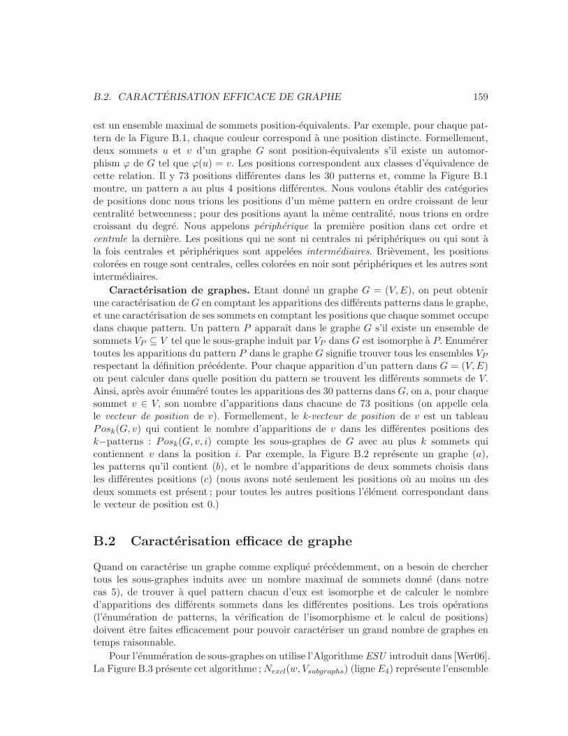
B.2. CARACTERISATION EFFICACE DE GRAPHE 159
est un ensemble maximal de sommets position-equivalents. Par exemple, pour chaque pat-tern de la Figure B.1, chaque couleur correspond a une position distincte. Formellement,deux sommets u et v d’un graphe G sont position-equivalents s’il existe un automor-phism ϕ de G tel que ϕ(u) = v. Les positions correspondent aux classes d’equivalence decette relation. Il y 73 positions differentes dans les 30 patterns et, comme la Figure B.1montre, un pattern a au plus 4 positions differentes. Nous voulons etablir des categoriesde positions donc nous trions les positions d’un meme pattern en ordre croissant de leurcentralite betweenness ; pour des positions ayant la meme centralite, nous trions en ordrecroissant du degre. Nous appelons peripherique la premiere position dans cet ordre etcentrale la derniere. Les positions qui ne sont ni centrales ni peripheriques ou qui sont ala fois centrales et peripheriques sont appelees intermediaires. Brievement, les positionscolorees en rouge sont centrales, celles colorees en noir sont peripheriques et les autres sontintermediaires.
Caracterisation de graphes. Etant donne un graphe G = (V,E), on peut obtenirune caracterisation de G en comptant les apparitions des differents patterns dans le graphe,et une caracterisation de ses sommets en comptant les positions que chaque sommet occupedans chaque pattern. Un pattern P apparaıt dans le graphe G s’il existe un ensemble desommets VP ⊆ V tel que le sous-graphe induit par VP dans G est isomorphe a P. Enumerertoutes les apparitions du pattern P dans le graphe G signifie trouver tous les ensembles VP
respectant la definition precedente. Pour chaque apparition d’un pattern dans G = (V,E)on peut calculer dans quelle position du pattern se trouvent les differents sommets de V.Ainsi, apres avoir enumere toutes les apparitions des 30 patterns dans G, on a, pour chaquesommet v ∈ V, son nombre d’apparitions dans chacune de 73 positions (on appelle celale vecteur de position de v). Formellement, le k-vecteur de position de v est un tableauPosk(G, v) qui contient le nombre d’apparitions de v dans les differentes positions desk−patterns : Posk(G, v, i) compte les sous-graphes de G avec au plus k sommets quicontiennent v dans la position i. Par exemple, la Figure B.2 represente un graphe (a),les patterns qu’il contient (b), et le nombre d’apparitions de deux sommets choisis dansles differentes positions (c) (nous avons note seulement les positions ou au moins un desdeux sommets est present ; pour toutes les autres positions l’element correspondant dansle vecteur de position est 0.)
B.2 Caracterisation efficace de graphe
Quand on caracterise un graphe comme explique precedemment, on a besoin de cherchertous les sous-graphes induits avec un nombre maximal de sommets donne (dans notrecas 5), de trouver a quel pattern chacun d’eux est isomorphe et de calculer le nombred’apparitions des differents sommets dans les differentes positions. Les trois operations(l’enumeration de patterns, la verification de l’isomorphisme et le calcul de positions)doivent etre faites efficacement pour pouvoir caracteriser un grand nombre de graphes entemps raisonnable.
Pour l’enumeration de sous-graphes on utilise l’Algorithme ESU introduit dans [Wer06].La Figure B.3 presente cet algorithme ;Nexcl(w, Vsubgraphs) (ligne E4) represente l’ensemble
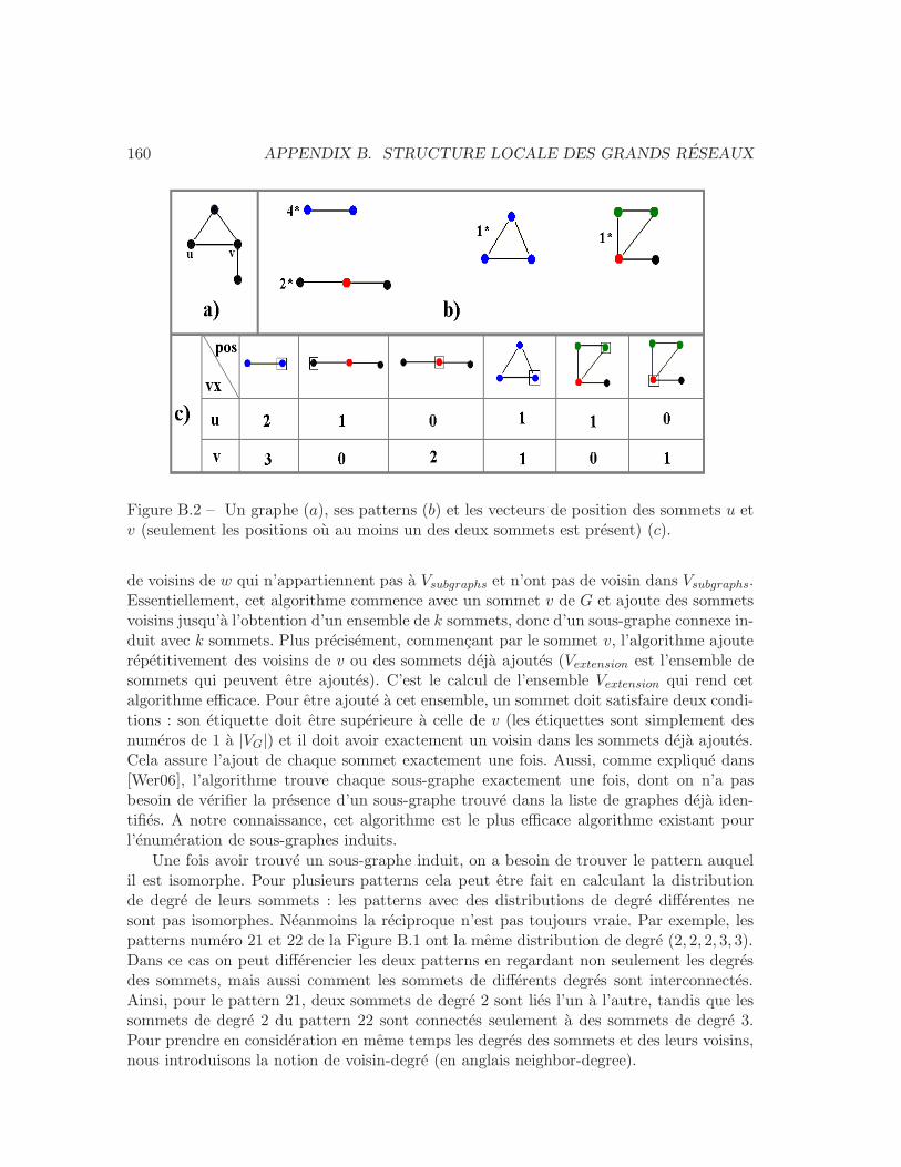
160 APPENDIX B. STRUCTURE LOCALE DES GRANDS RESEAUX
Figure B.2 – Un graphe (a), ses patterns (b) et les vecteurs de position des sommets u etv (seulement les positions ou au moins un des deux sommets est present) (c).
de voisins de w qui n’appartiennent pas a Vsubgraphs et n’ont pas de voisin dans Vsubgraphs.Essentiellement, cet algorithme commence avec un sommet v de G et ajoute des sommetsvoisins jusqu’a l’obtention d’un ensemble de k sommets, donc d’un sous-graphe connexe in-duit avec k sommets. Plus precisement, commencant par le sommet v, l’algorithme ajouterepetitivement des voisins de v ou des sommets deja ajoutes (Vextension est l’ensemble desommets qui peuvent etre ajoutes). C’est le calcul de l’ensemble Vextension qui rend cetalgorithme efficace. Pour etre ajoute a cet ensemble, un sommet doit satisfaire deux condi-tions : son etiquette doit etre superieure a celle de v (les etiquettes sont simplement desnumeros de 1 a |VG|) et il doit avoir exactement un voisin dans les sommets deja ajoutes.Cela assure l’ajout de chaque sommet exactement une fois. Aussi, comme explique dans[Wer06], l’algorithme trouve chaque sous-graphe exactement une fois, dont on n’a pasbesoin de verifier la presence d’un sous-graphe trouve dans la liste de graphes deja iden-tifies. A notre connaissance, cet algorithme est le plus efficace algorithme existant pourl’enumeration de sous-graphes induits.
Une fois avoir trouve un sous-graphe induit, on a besoin de trouver le pattern auquelil est isomorphe. Pour plusieurs patterns cela peut etre fait en calculant la distributionde degre de leurs sommets : les patterns avec des distributions de degre differentes nesont pas isomorphes. Neanmoins la reciproque n’est pas toujours vraie. Par exemple, lespatterns numero 21 et 22 de la Figure B.1 ont la meme distribution de degre (2, 2, 2, 3, 3).Dans ce cas on peut differencier les deux patterns en regardant non seulement les degresdes sommets, mais aussi comment les sommets de differents degres sont interconnectes.Ainsi, pour le pattern 21, deux sommets de degre 2 sont lies l’un a l’autre, tandis que lessommets de degre 2 du pattern 22 sont connectes seulement a des sommets de degre 3.Pour prendre en consideration en meme temps les degres des sommets et des leurs voisins,nous introduisons la notion de voisin-degre (en anglais neighbor-degree).
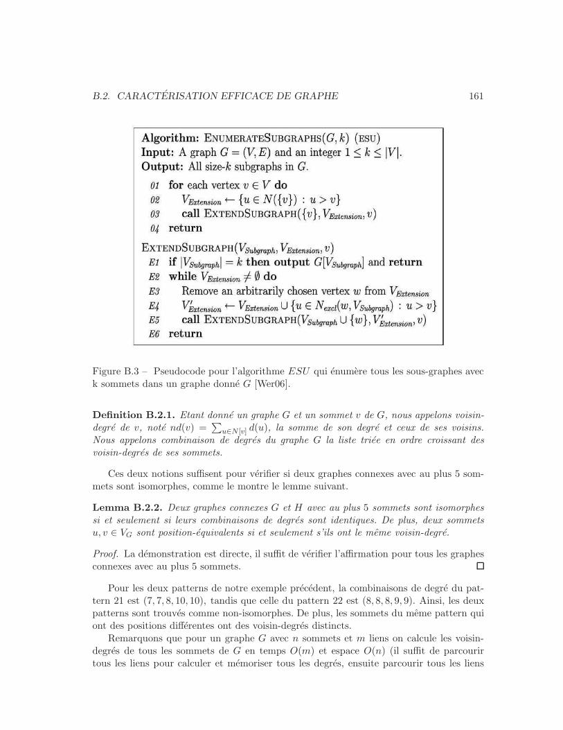
B.2. CARACTERISATION EFFICACE DE GRAPHE 161
Figure B.3 – Pseudocode pour l’algorithme ESU qui enumere tous les sous-graphes aveck sommets dans un graphe donne G [Wer06].
Definition B.2.1. Etant donne un graphe G et un sommet v de G, nous appelons voisin-degre de v, note nd(v) =
∑
u∈N [v] d(u), la somme de son degre et ceux de ses voisins.Nous appelons combinaison de degres du graphe G la liste triee en ordre croissant desvoisin-degres de ses sommets.
Ces deux notions suffisent pour verifier si deux graphes connexes avec au plus 5 som-mets sont isomorphes, comme le montre le lemme suivant.
Lemma B.2.2. Deux graphes connexes G et H avec au plus 5 sommets sont isomorphessi et seulement si leurs combinaisons de degres sont identiques. De plus, deux sommetsu, v ∈ VG sont position-equivalents si et seulement s’ils ont le meme voisin-degre.
Proof. La demonstration est directe, il suffit de verifier l’affirmation pour tous les graphesconnexes avec au plus 5 sommets.
Pour les deux patterns de notre exemple precedent, la combinaisons de degre du pat-tern 21 est (7, 7, 8, 10, 10), tandis que celle du pattern 22 est (8, 8, 8, 9, 9). Ainsi, les deuxpatterns sont trouves comme non-isomorphes. De plus, les sommets du meme pattern quiont des positions differentes ont des voisin-degres distincts.
Remarquons que pour un graphe G avec n sommets et m liens on calcule les voisin-degres de tous les sommets de G en temps O(m) et espace O(n) (il suffit de parcourirtous les liens pour calculer et memoriser tous les degres, ensuite parcourir tous les liens
162 APPENDIX B. STRUCTURE LOCALE DES GRANDS RESEAUX
Figure B.4 – Deux graphes connexes non-isomorphes avec 6 sommets.
de nouveau pour calculer les voisin-degres), ensuite sa combinaison de degre en tempsO(n · logn). Pour l’ensemble de patterns ces quantites sont constantes comme n et m sontau plus 5, respectivement 10. Donc on peut trouver a quel pattern un graphe connexe avecau plus 5 sommets correspond (i.e. auquel des 30 graphes de la Figure B.1 il est isomorphe)et verifier si deux de ses sommets sont equivalents en temps constant.
Toutefois le lemme n’est pas valable pour les graphes connexes avec 6 sommets. Lesdeux graphes de la Figure B.4 ne sont pas isomorphes mais ont la meme combinaison dedegres : (7, 7, 7, 7, 10, 10).
B.3 Une methode pour l’analyse de la structure locale
Etant donne un graphe (eventuellement grand) G = (V,E), nous nous proposons d’analy-ser sa structure locale autour d’un sommet v ∈ V (nous appelons ce sommet ego). Nousprocedons comme il suit – methode structure locale(v) :
Etape 1. Extraire le reseau egocentre Eg(v) de v i.e. le sous-graphe induit par les voisinsde v dans G ;
Etape 2. Enumerer les patterns de Eg(v) ;
Etape 3. Calculer les vecteurs de position des sommets de Eg(v).
Nous expliquons les trois etapes de la methode avec un exemple.Etapes 1 et 2. Dans la Figure B.5(a), les cercles noirs correspondent aux voisins de
v, les traits noirs correspondent aux liens entre eux et les traits rouges aux liens entrev et ses voisins. Le reseau egocentre Eg(v) de v est represente dans la Figure B.5(b) etles patterns de Eg(v) dans la Figure B.5(c) 1. Nous choisissons de ne pas inclure v dansson reseau egocentre parce que nous savons qu’il est connecte a tous les sommets de cegraphe, sa presence n’apporte aucune information. Apres avoir effectue les deux premierspas de la methode, on a une description riche de la facon dont v est connecte au grapheG. Pour une description plus detaillee de la structure locale de G on peut enumerer lespatterns d’un plus grand ordre (avec plus de 5 sommets) ; les patterns avec 5 sommets
1 Nous avons aussi compte les sommets et les liens isoles de Eg(v).
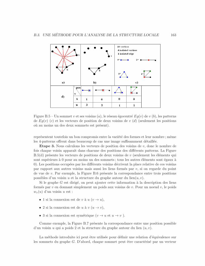
B.3. UNE METHODE POUR L’ANALYSE DE LA STRUCTURE LOCALE 163
Figure B.5 – Un sommet v et ses voisins (a), le reseau egocentre Eg(v) de v (b), les patternsde Eg(v) (c) et les vecteurs de position de deux voisins de v (d) (seulement les positionsou au moins un des deux sommets est present).
representent toutefois un bon compromis entre la variete des formes et leur nombre ; memeles 4-patterns offrent dans beaucoup de cas une image suffisamment detaillee.
Etape 3. Nous calculons les vecteurs de position des voisins de v, donc le nombre defois chaque voisin apparaıt dans chacune des positions des differents patterns. La FigureB.5(d) presente les vecteurs de positions de deux voisins de v (seulement les elements quisont superieurs a 0 pour au moins un des sommets ; tous les autres elements sont egaux a0). Les positions occupees par les differents voisins decrivent la place relative de ces voisinspar rapport aux autres voisins mais aussi les liens formes par v, si on regarde du pointde vue de v. Par exemple, la Figure B.6 presente la correspondance entre trois positionspossibles d’un voisin u et la structure du graphe autour du lien(u, v).
Si le graphe G est dirige, on peut ajouter cette information a la description des liensformes par v en donnant simplement un poids aux voisins de v. Pour un noeud v, le poidswv(u) d’un voisin u est :
• 1 si la connexion est de v a u (v → u),
• 2 si la connexion est de u a v (u→ v),
• 3 si la connexion est symetrique (v → u et u→ v ).
Comme exemple, la Figure B.7 presente la correspondance entre une position possibled’un voisin u qui a poids 2 et la structure du graphe autour du lien (u, v).
La methode introduite ici peut etre utilisee pour definir une relation d’equivalence surles sommets du graphe G. D’abord, chaque sommet peut etre caracterise par un vecteur
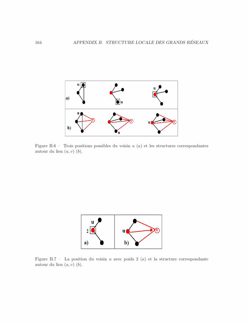
164 APPENDIX B. STRUCTURE LOCALE DES GRANDS RESEAUX
Figure B.6 – Trois positions possibles du voisin u (a) et les structures correspondantesautour du lien (u, v) (b).
Figure B.7 – La position du voisin u avec poids 2 (a) et la structure correspondanteautour du lien (u, v) (b).
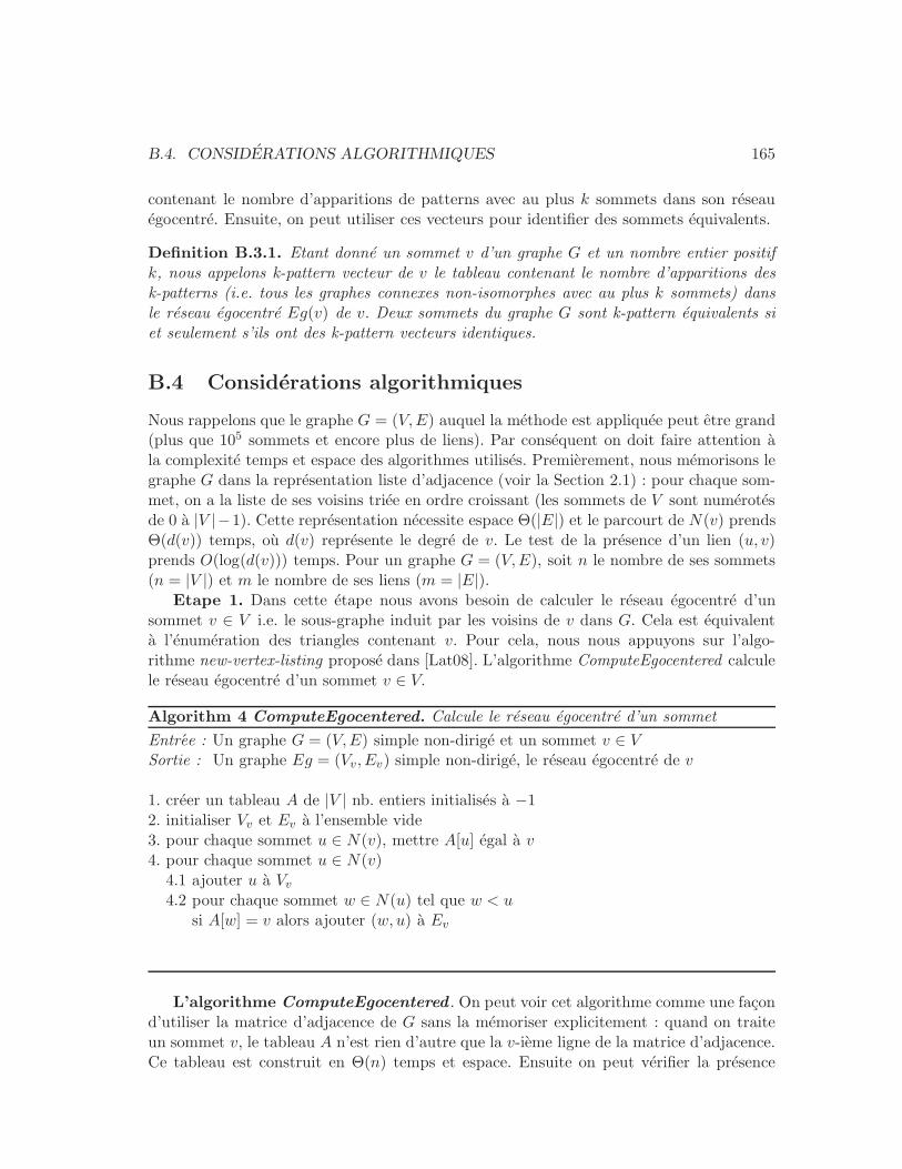
B.4. CONSIDERATIONS ALGORITHMIQUES 165
contenant le nombre d’apparitions de patterns avec au plus k sommets dans son reseauegocentre. Ensuite, on peut utiliser ces vecteurs pour identifier des sommets equivalents.
Definition B.3.1. Etant donne un sommet v d’un graphe G et un nombre entier positifk, nous appelons k-pattern vecteur de v le tableau contenant le nombre d’apparitions desk-patterns (i.e. tous les graphes connexes non-isomorphes avec au plus k sommets) dansle reseau egocentre Eg(v) de v. Deux sommets du graphe G sont k-pattern equivalents siet seulement s’ils ont des k-pattern vecteurs identiques.
B.4 Considerations algorithmiques
Nous rappelons que le graphe G = (V,E) auquel la methode est appliquee peut etre grand(plus que 105 sommets et encore plus de liens). Par consequent on doit faire attention ala complexite temps et espace des algorithmes utilises. Premierement, nous memorisons legraphe G dans la representation liste d’adjacence (voir la Section 2.1) : pour chaque som-met, on a la liste de ses voisins triee en ordre croissant (les sommets de V sont numerotesde 0 a |V |−1). Cette representation necessite espace Θ(|E|) et le parcourt de N(v) prendsΘ(d(v)) temps, ou d(v) represente le degre de v. Le test de la presence d’un lien (u, v)prends O(log(d(v))) temps. Pour un graphe G = (V,E), soit n le nombre de ses sommets(n = |V |) et m le nombre de ses liens (m = |E|).
Etape 1. Dans cette etape nous avons besoin de calculer le reseau egocentre d’unsommet v ∈ V i.e. le sous-graphe induit par les voisins de v dans G. Cela est equivalenta l’enumeration des triangles contenant v. Pour cela, nous nous appuyons sur l’algo-rithme new-vertex-listing propose dans [Lat08]. L’algorithme ComputeEgocentered calculele reseau egocentre d’un sommet v ∈ V.
Algorithm 4 ComputeEgocentered. Calcule le reseau egocentre d’un sommet
Entree : Un graphe G = (V,E) simple non-dirige et un sommet v ∈ VSortie : Un graphe Eg = (Vv, Ev) simple non-dirige, le reseau egocentre de v
1. creer un tableau A de |V | nb. entiers initialises a −12. initialiser Vv et Ev a l’ensemble vide3. pour chaque sommet u ∈ N(v), mettre A[u] egal a v4. pour chaque sommet u ∈ N(v)
4.1 ajouter u a Vv
4.2 pour chaque sommet w ∈ N(u) tel que w < usi A[w] = v alors ajouter (w, u) a Ev
L’algorithme ComputeEgocentered . On peut voir cet algorithme comme une facond’utiliser la matrice d’adjacence de G sans la memoriser explicitement : quand on traiteun sommet v, le tableau A n’est rien d’autre que la v-ieme ligne de la matrice d’adjacence.Ce tableau est construit en Θ(n) temps et espace. Ensuite on peut verifier la presence
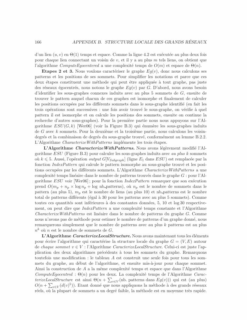
166 APPENDIX B. STRUCTURE LOCALE DES GRANDS RESEAUX
d’un lien (u, v) en Θ(1) temps et espace. Comme la ligne 4.2 est executee au plus deux foispour chaque lien connectant un voisin de v, et il y a au plus m tels liens, on obtient quel’algorithme ComputeEgocentered a une complexite temps de O(m) et espace de Θ(n).
Etapes 2 et 3. Nous voulons caracteriser le graphe Eg(v), donc nous calculons sespatterns et les positions de ses sommets. Pour simplifier les notations et parce que cesdeux etapes constituent une methode qui peut etre appliquee a tout graphe, pas justedes reseaux egocentres, nous notons le graphe Eg(v) par G. D’abord, nous avons besoind’identifier les sous-graphes connexes induits avec au plus 5 sommets de G, ensuite detrouver le pattern auquel chacun de ces graphes est isomorphe et finalement de calculerles positions occupees par les differents sommets dans le sous-graphe identifie (en fait lestrois operations sont successives : une fois avoir trouve le sous-graphe, on verifie a quelpattern il est isomorphe et on calcule les positions des sommets, ensuite on continue larecherche d’autres sous-graphes). Pour la premiere partie nous nous appuyons sur l’Al-gorithme ESU(G, k) [Wer06] (voir la Figure B.3) qui enumere les sous-graphes induitsde G avec k sommets. Pour la deuxieme et la troisieme partie, nous calculons les voisin-degres et la combinaison de degres du sous-graphe trouve, conformement au lemme B.2.2.L’Algorithme CharacterizeWithPatterns implemente les trois etapes.
L’Algorithme CharacterizeWithPatterns. Nous avons legerement modifie l’Al-gorithme ESU (Figure B.3) pour calculer les sous-graphes induits avec au plus k sommetsou k 6 5. Aussi, l’operation output G[VSubgraph] (ligne E1 dans ESU) est remplacee par lafonction IndexPattern qui calcule le pattern isomorphe au sous-graphe trouve et les posi-tions occupees par les differents sommets. L’Algorithme CharacterizeWithPatterns a unecomplexite temps lineaire dans le nombre de patterns trouves dans le graphe G : pour l’Al-gorithme ESU voir [Wer06] ; pour la fonction IndexPattern remarquer que son executionprend O(mp + np × log np + log nb patterns), ou np est le nombre de sommets dans lepattern (au plus 5), mp est le nombre de liens (au plus 10) et nb patterns est le nombretotal de patterns differents (egal a 30 pour les patterns avec au plus 5 sommets). Commetoutes ces quantites sont inferieures a des constantes donnees, 5, 10 et log 30 respective-ment, on peut dire que IndexPattern a une complexite temps constante et l’AlgorithmeCharacterizeWithPatterns est lineaire dans le nombre de patterns du graphe G. Commenous n’avons pas de methode pour estimer le nombre de patterns d’un graphe donne, nousremarquerons simplement que le nombre de patterns avec au plus k patterns est au plusnk ou n est le nombre de sommets de G.
L’Algorithme CaracterizeLocalStructure.Nous avons maintenant tous les elementspour ecrire l’algorithme qui caracterise la structure locale du graphe G = (V,E) autourde chaque sommet v ∈ V : l’Algorithme CaracterizeLocalStructure. Celui-ci est juste l’ap-plication des deux algorithmes precedents a tous les sommets du graphe. Remarquonstoutefois une modification : le tableau A est construit une seule fois pour tous les som-mets du graphe, au debut de l’algorithme, et ensuite mis-a-jour pour chaque sommet.Ainsi la construction de A a la meme complexite temps et espace que dans l’AlgorithmeComputeEgocentred : Θ(n) pour les deux. La complexite temps de l’Algorithme Carac-terizeLocalStructure est ainsi Θ(n +
∑
v∈V (nb. patterns dans Eg(v))) qui est (au plus)O(n+
∑
v∈V (d(v)5)). Etant donne que nous appliquons la methode a des grands reseaux
reels, ou la plupart de sommets a un degre faible, la methode est en moyenne tres rapide.

B.4. CONSIDERATIONS ALGORITHMIQUES 167
Algorithm 5 CharacterizeWithPatterns. Caracterise un graphe simple non-dirige
Entree : Un graphe simple non-dirige G = (V,E) et un nombre entier positif k 6 5Sortie : Un tableau Pt tel que Pt[P ] contient le nb. d’occurrences du pattern P dans G,un tableau Ps tel que Ps[v][i] = Posk(G, v, i) (le nb. d’occurrences de v dans la position i)
1. mettre tous les elements de Pt et Ps a 02. pour chaque sommet v ∈ V faire
2.1 Vextension ←− {u ∈ N(v) : u > v}2.2 VSubgraph = {v}, ESubgraph = ∅2.3 appeler ExtendSubgraph(VSubgraph, ESubgraph, VExtension, v, P t, Ps, k)
3. retourner
ExtendSubgraphEntree :- un nombre entier positif k 6 5,- deux ensembles VSubgraph ⊆ V et ESubgraph ⊆ E contenant les sommets et les liensdeja ajoutes au sous-graphe,
- un ensemble de sommets Vextension contenant les sommets qui peuvent etre ajoutes au sous-graphe,- un sommet v ou la construction du graphe a commence,- deux tableaux Pt et Ps qui seront mis-a-jour par la procedure
1. si |VSubgraph| > k retourner2. si |VSubgraph| > 0 appeler IndexPattern(VSubgraph, ESubgraph,Pt, Ps )3. tant que VExtension 6= ∅
3.1. prendre un sommet w choisi aleatoirement dans VExtension
3.2. V ′Extension = VExtension
3.3. E′Subgraph = ESubgraph
3.4. pour chaque u ∈ N(w) : u > vsi u ∈ VSubgraph ajouter (u,w) a E′
Subgraph //ajouter tous les liens de w vers le sous-graphe
sinon si u /∈ N(VSubgraph) ajouter u a V ′Extension
3.5. appeler ExtendSubgraph(VSubgraph ∪ {w} , E′Subgraph, V
′Extension, v, P t, Ps, k )
IndexPatternEntree : Un ensemble de sommets VSubgraph, un ensemble de liens ESubgraph etdeux tableaux Pt et Ps qui seront mis-a-jour par la procedure
1. parcourir l’ensemble ESubgraph et noter chaque occurrence de chaque sommet//ainsi calculant les degres des sommets
2. creer un tableau D contenant les degres des sommets3. pour chaque lien (a, b) ∈ ESubgraph ajouter degre(b) a D(a) et degre(a) a D(b)
// ainsi calculant les voisin-degres4. trier D et l’ecrire comme un nombre5. trouver le pattern P avec ce numero et incrementer Pt(P )6. pour chaque sommet u
trouver la position i (dans le pattern P ) avec le meme voisin-degre et incrementer Ps[u][i]
168 APPENDIX B. STRUCTURE LOCALE DES GRANDS RESEAUX
Dans le Chapitre 7 nous appliquons la methode a un graphe reel avec 2.7M sommets et6.4M liens et nous donnons une complexite empirique de notre methode pour ce graphe-la. L’execution de notre implementation C++ de la methode prend 31 minutes sur unordinateur de configuration standard avec un processeur de 2.8GHz et 4Go RAM.
Algorithm 6 CaracterizeLocalStructure. Caracterise la structure locale autour dechaque sommet dans un (grand) graphe
Entree : Un graphe simple non-dirige G = (V,E) et un nombre entier positif k 6 5
1. creer un tableau A de |V | nombres entiers et les mettre a −12. pour chaque sommet v ∈ V
2.1 initialiser Vv et Ev a l’ensemble vide2.2 pour chaque sommet u dans N(v), mettre A[u] a v2.3 pour chaque sommet u dans N(v)
2.3.1 ajouter u a Vv
2.3.2 pour chaque sommet w dans N(u) tel que w < usi A[w] = v alors ajouter (w, u) a Ev
2.4 appeler CharacterizeWithPatterns((Vv , Ev), k)
B.5 Applications de la methode
Le but de la methode que nous avons presentee ici est de caracteriser la facon dont unsommet est connecte au reseau. C’est une methode pour l’analyse de la structure localedu reseau qui produit une caracterisation de chaque sommet. Son but n’est pas de don-ner un classement ou un ordre de sommets, mais simplement de montrer comment ilssont connectes au reseau. Cela peut etre utile dans plusieurs situations. D’abord, commen’importe quelle methode de caracterisation, il ameliore notre connaissance des sommetsdu reseau. Deuxiemement, la caracterisation des sommets obtenue peut etre comparee ad’autres proprietes des sommets : s’il y a une correlation, on peut utiliser l’une pour prevoirles autres. Cela est pratique quand il y a des donnees manquantes parce que quelques unesdes proprietes peuvent etre deduites des autres. Troisiemement, il y a des situations ouune analyse locale est la meilleure facon d’etudier le probleme. C’est le cas des donneesobtenues independamment pour des personnes differentes, ou le reseau ”global” contenanttoutes les personnes est inconnu (comme par exemple dans le cas des etudes sociologiquesou les donnees sur chaque personne sont obtenues par des entretiens individuels et il n’ya aucune collection du reseau entier). Dans ce cas on peut vouloir etudier le reseau danslequel les individus sont inclus, mais, comme il n’y a aucun reseau global, on ne peut pasfaire une analyse de reseau globale ou intermediaire classique.
Une autre situation ou l’etude de la structure locale est appropriee ce sont les reseauxou ”l’importance” des noeuds est locale. Dans la situation opposee, il y a des reseaux oucertains noeuds sont importants pour le fonctionnement du reseau entier. Prenons par
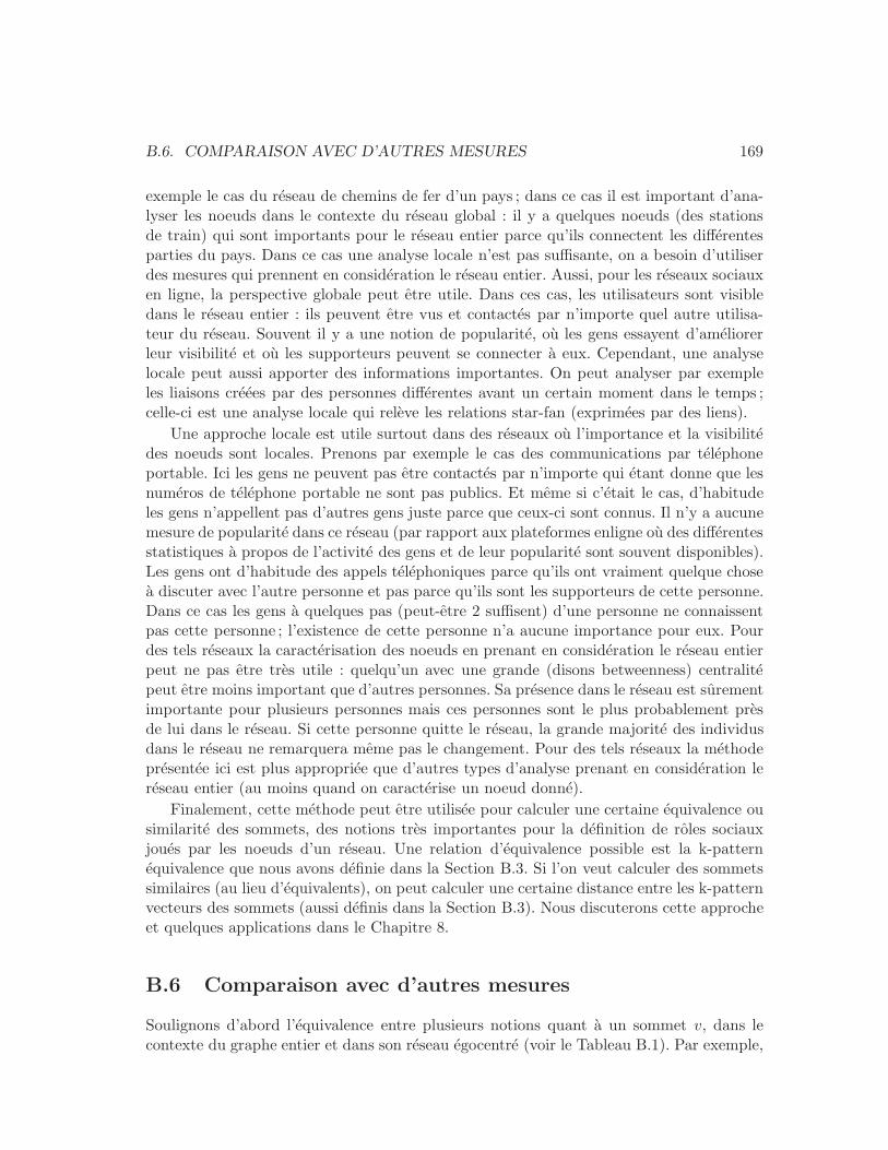
B.6. COMPARAISON AVEC D’AUTRES MESURES 169
exemple le cas du reseau de chemins de fer d’un pays ; dans ce cas il est important d’ana-lyser les noeuds dans le contexte du reseau global : il y a quelques noeuds (des stationsde train) qui sont importants pour le reseau entier parce qu’ils connectent les differentesparties du pays. Dans ce cas une analyse locale n’est pas suffisante, on a besoin d’utiliserdes mesures qui prennent en consideration le reseau entier. Aussi, pour les reseaux sociauxen ligne, la perspective globale peut etre utile. Dans ces cas, les utilisateurs sont visibledans le reseau entier : ils peuvent etre vus et contactes par n’importe quel autre utilisa-teur du reseau. Souvent il y a une notion de popularite, ou les gens essayent d’ameliorerleur visibilite et ou les supporteurs peuvent se connecter a eux. Cependant, une analyselocale peut aussi apporter des informations importantes. On peut analyser par exempleles liaisons creees par des personnes differentes avant un certain moment dans le temps ;celle-ci est une analyse locale qui releve les relations star-fan (exprimees par des liens).
Une approche locale est utile surtout dans des reseaux ou l’importance et la visibilitedes noeuds sont locales. Prenons par exemple le cas des communications par telephoneportable. Ici les gens ne peuvent pas etre contactes par n’importe qui etant donne que lesnumeros de telephone portable ne sont pas publics. Et meme si c’etait le cas, d’habitudeles gens n’appellent pas d’autres gens juste parce que ceux-ci sont connus. Il n’y a aucunemesure de popularite dans ce reseau (par rapport aux plateformes enligne ou des differentesstatistiques a propos de l’activite des gens et de leur popularite sont souvent disponibles).Les gens ont d’habitude des appels telephoniques parce qu’ils ont vraiment quelque chosea discuter avec l’autre personne et pas parce qu’ils sont les supporteurs de cette personne.Dans ce cas les gens a quelques pas (peut-etre 2 suffisent) d’une personne ne connaissentpas cette personne ; l’existence de cette personne n’a aucune importance pour eux. Pourdes tels reseaux la caracterisation des noeuds en prenant en consideration le reseau entierpeut ne pas etre tres utile : quelqu’un avec une grande (disons betweenness) centralitepeut etre moins important que d’autres personnes. Sa presence dans le reseau est surementimportante pour plusieurs personnes mais ces personnes sont le plus probablement presde lui dans le reseau. Si cette personne quitte le reseau, la grande majorite des individusdans le reseau ne remarquera meme pas le changement. Pour des tels reseaux la methodepresentee ici est plus appropriee que d’autres types d’analyse prenant en consideration lereseau entier (au moins quand on caracterise un noeud donne).
Finalement, cette methode peut etre utilisee pour calculer une certaine equivalence ousimilarite des sommets, des notions tres importantes pour la definition de roles sociauxjoues par les noeuds d’un reseau. Une relation d’equivalence possible est la k-patternequivalence que nous avons definie dans la Section B.3. Si l’on veut calculer des sommetssimilaires (au lieu d’equivalents), on peut calculer une certaine distance entre les k-patternvecteurs des sommets (aussi definis dans la Section B.3). Nous discuterons cette approcheet quelques applications dans le Chapitre 8.
B.6 Comparaison avec d’autres mesures
Soulignons d’abord l’equivalence entre plusieurs notions quant a un sommet v, dans lecontexte du graphe entier et dans son reseau egocentre (voir le Tableau B.1). Par exemple,
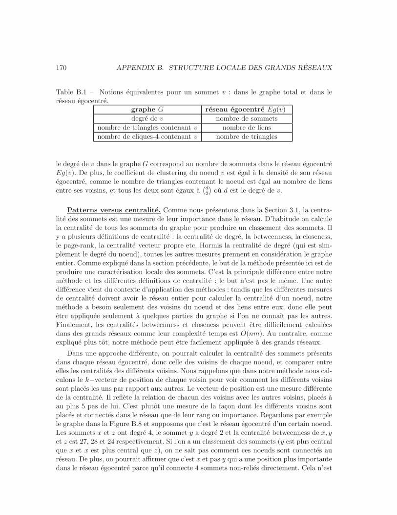
170 APPENDIX B. STRUCTURE LOCALE DES GRANDS RESEAUX
Table B.1 – Notions equivalentes pour un sommet v : dans le graphe total et dans lereseau egocentre.
graphe G reseau egocentre Eg(v)
degre de v nombre de sommets
nombre de triangles contenant v nombre de liens
nombre de cliques-4 contenant v nombre de triangles
le degre de v dans le graphe G correspond au nombre de sommets dans le reseau egocentreEg(v). De plus, le coefficient de clustering du noeud v est egal a la densite de son reseauegocentre, comme le nombre de triangles contenant le noeud est egal au nombre de liensentre ses voisins, et tous les deux sont egaux a
(
d2
)
ou d est le degre de v.
Patterns versus centralite. Comme nous presentons dans la Section 3.1, la centra-lite des sommets est une mesure de leur importance dans le reseau. D’habitude on calculela centralite de tous les sommets du graphe pour produire un classement des sommets. Ily a plusieurs definitions de centralite : la centralite de degre, la betweenness, la closeness,le page-rank, la centralite vecteur propre etc. Hormis la centralite de degre (qui est sim-plement le degre du noeud), toutes les autres mesures prennent en consideration le grapheentier. Comme explique dans la section precedente, le but de la methode presentee ici est deproduire une caracterisation locale des sommets. C’est la principale difference entre notremethode et les differentes definitions de centralite : le but n’est pas le meme. Une autredifference vient du contexte d’application des methodes : tandis que les differentes mesuresde centralite doivent avoir le reseau entier pour calculer la centralite d’un noeud, notremethode a besoin seulement des voisins du noeud et des liens entre eux, donc elle peutetre appliquee seulement a quelques parties du graphe si l’on ne connaıt pas les autres.Finalement, les centralites betweenness et closeness peuvent etre difficilement calculeesdans des grands reseaux comme leur complexite temps est O(nm). Au contraire, commeexplique plus tot, notre methode peut etre facilement appliquee a des grands reseaux.
Dans une approche differente, on pourrait calculer la centralite des sommets presentsdans chaque reseau egocentre, donc celle des voisins de chaque noeud, et comparer entreelles les centralites des differents voisins. Nous rappelons que dans notre methode nous cal-culons le k−vecteur de position de chaque voisin pour voir comment les differents voisinssont places les uns par rapport aux autres. Le vecteur de position est une mesure differentede la centralite. Il reflete la relation de chacun des voisins avec les autres voisins, places aau plus 5 pas de lui. C’est plutot une mesure de la facon dont les differents voisins sontplaces et connectes dans le reseau que de leur rang ou importance. Regardons par exemplele graphe dans la Figure B.8 et supposons que c’est le reseau egocentre d’un certain noeud.Les sommets x et z ont degre 4, le sommet y a degre 2 et la centralite betweenness de x, yet z est 27, 28 et 24 respectivement. Si l’on a un classement des sommets (y est plus centralque x et x est plus central que z), on ne sait pas comment ces noeuds sont connectes aureseau. De plus, on pourrait affirmer que c’est x et pas y qui a une position plus importantedans le reseau egocentre parce qu’il connecte 4 sommets non-relies directement. Cela n’est
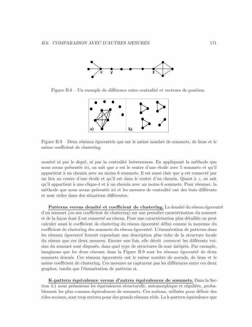
B.6. COMPARAISON AVEC D’AUTRES MESURES 171
Figure B.8 – Un exemple de difference entre centralite et vecteurs de position.
Figure B.9 – Deux reseaux egocentres qui ont le meme nombre de sommets, de liens et lememe coefficient de clustering.
montre ni par le degre, ni par la centralite betweenness. En appliquant la methode quenous avons presentee ici, on sait que x est le centre d’une etoile avec 5 sommets et qu’ilappartient a un chemin avec au moins 6 sommets. Il est aussi clair que y est connecte parun lien au centre d’une etoile et qu’il est dans le centre d’un chemin. Quant a z, on saitqu’il appartient a une clique-4 et a un chemin avec au moins 6 sommets. Pour resumer, lamethode que nous avons presentee ici et les mesures de centralite ont des buts differentset sont utiles dans des situations differentes.
Patterns versus densite et coefficient de clustering. La densite du reseau egocentred’un sommet (ou son coefficient de clustering) est une premiere caracterisation du sommetet de la facon dont il est connecte au reseau. Pour une caracterisation plus detaillee on peutcalculer aussi le coefficient de clustering du reseau egocentre defini comme la moyenne ducoefficient de clustering des sommets du reseau egocentre. L’enumeration de patterns dansles reseaux egocentre fournit cependant une description plus riche de la structure localedu reseau que ces deux mesures. Encore une fois, elle decrit comment les differents voi-sins du sommet sont disposes, dans quel type de structures ils sont integres. Par exemple,imaginons que les deux reseaux dans la Figure B.9 sont les reseaux egocentre de deuxsommets donnes. Ces reseaux egocentres ont le meme nombre de noeuds, de liens et lememe coefficient de clustering. Ces mesures ne capturent pas les differences entre ces deuxgraphes, tandis que l’enumeration de patterns si.
K-pattern equivalence versus d’autres equivalences de sommets. Dans la Sec-tion 4.1 nous presentons les equivalences structurelle, automorphique et reguliere, proba-blement les plus connues equivalences de sommets. Ces notions, utilisees pour definir desroles sociaux, sont trop strictes pour des grands reseaux reels. La k-pattern equivalence que
172 APPENDIX B. STRUCTURE LOCALE DES GRANDS RESEAUX
nous avons definie dans la Section B.3 est incluse dans l’equivalence structurelle et auto-morphique. Cela s’appuie sur les observations simples que les sommets qui ont exactementles memes voisins dans le reseau (donc sont structurellement equivalents) ont des reseauxegocentres identiques, donc des vecteurs de parametres (en anglais feature vectors) iden-tiques et sont donc k-pattern equivalents, pour tout k. Aussi, les sommets automorphique-ment equivalents ont des reseaux egocentre isomorphes, donc des vecteurs de parametresidentiques et sont ainsi k-pattern equivalents, pour tout k. Pour les deux definitions, lareciproque n’est pas toujours vraie, donc on peut dire que la k-pattern equivalence estincluse dans les equivalences structurelle et automorphique. Cela signifie que la k-patternequivalence est moins stricte que ces deux relations ; cependant elle n’est toujours pas assezflexible pour des reseaux reels. Quelques adaptations des k-pattern vecteurs pour calculerla similarite des sommets dans des graphes de terrain seront discutees dans le Chapitre 8.
B.7 Conclusions du chapitre
Nous avons presente dans ce chapitre une methode pour l’analyse de la structure localed’un graphe autour de chaque sommet. Cette methode fournit une description riche de lafacon dont un noeud donne est connecte au graphe et aussi de la facon dont ses voisinssont places les uns par rapport aux autres. Elle peut etre appliquee aussi bien a des petitsreseaux qu’a des grands et meme a des fractions de reseaux. Dans les chapitres suivantsnous appliquons cette methode a deux reseaux sociaux, le premier modelisant l’activitesur une plateforme enligne et le deuxieme modelisant des communications par telephoneportable. Dans le premier cas nous etudions la relation entre la popularite d’utilisateurset la structure du reseau dans lequel ils sont integres, tandis que dans le deuxieme casnous comparons la facon dont les sommets et leurs voisins sont places dans le graphea d’autres informations (age, sexe, intensite de communication) sur les utilisateurs detelephone portable.
Index
Aadjacency
adjacency list, 38, 92adjacency matrix, 38, 51, 59, 93
automorphism, 38, 87
Bbreadth-first search, 38, 52, 55, 75, 102
Ccentrality, 53, 97
betweenness, 55, 87, 97closeness, 55, 97degree centrality, 55, 97eigen vector, 55, 97page rank, 55, 97
classification, 42cluster
center, 40, 138clustering, 39, 130, 137
hierarchical clustering, 41, 142clustering coefficient, 50, 57, 97, 98, 117community, 53, 76complexity, 38, 118connected component, 37, 52, 77, 117correlation, 43, 102
Pearson correlation, 43covariance, 43cycle, 37
Ddecision tree, 43, 147degree, 37, 50, 55
degree combination, 88, 93degree distribution, 46, 60, 71, 76, 79,
117neighbor-degree, 88, 93
density, 38, 76, 97, 98
depth-first search, 38, 60
diameter, 38, 48, 77
average diameter, 49, 77
effective diameter, 48, 77
distance, 37, 65
Euclidian distance, 40, 133
Manhattan distance, 40
E
ego, 68, 123, 145
egocentred network, 85, 106, 117, 131
equivalence
automorphic equivalence, 67, 85, 99
k-pattern equivalence, 97, 99, 130
pattern-frequency equivalence, 133
position equivalence, 85
regular equivalence, 68, 99
structural equivalence, 66, 99
Erdos-Renyi model, 46, 57
F
feature vector, 39
G
graph, 37
complement graph, 37, 137
directed graph, 37
random graph, 46, 58, 60, 72
simple graph, 37
H
hop-plot, 49
I
isomorphism, 38, 59
173
174 INDEX
K
k-means, 40, 137, 138, 152k-nearest neighbors, 42k-pattern vector, 92, 97, 130Kohonen SOM, 41, 103, 149
Llinear regression, 43lognormal distribution, 48
Nneighbor, 37, 85
neighbor-degree, 88, 93
neighborhood, 37network
network closure, 65
network model, 57network motifs, 60, 120
P
p-value, 44, 145path, 37, 55, 57
characteristic path length, 49path length, 37
patterns, 85, 106, 117frequent patterns, 59, 120k-patterns, 85
PCA, 41position, 85
central, 87, 109, 124
intermediate, 87, 109, 124peripheral, 87, 109, 124position equivalence, 85
position vector, 87, 109, 117power-law, 46, 51, 58, 76
exponential cutoff, 47
preferential attachment, 57, 77
Rroles, 66, 99, 130
Ssmall world, 50, 65social capital, 65, 76
standard deviation, 43, 135
strength of ties, 65structural holes, 65subgraph, 38, 59, 60
induced subgraph, 38, 85
Ttest
χ2 test, 44, 145ANOVA test, 44, 145hypothesis test, 44Mantel test, 102multiple comparison test, 44, 146
transitivity ratio, 51triangle, 38, 50, 58, 93, 117, 131
Related Documents