Analyzing the Effects of FACTS Devices

By:

Ibrahem M. Hussein ID: 201405220

Date: 25-12-2014

2014

KING FAHD UNIVERSITY OF

PETROLEM AND MINERALS ELECTRICAL ENGINEERING DEPARTMENT

Electrical Transmission ,EE-525

Term-Paper

[ Analyzing the Effects of FACTS Devices on Steady

State Performance of Hydro-Quebec Network ]

Instructor: Dr. Chokri B. Ahmad

2

Table of Contents

List of Figures……………………………………………………2

List of Tables ………………………………………….…………2

Abstract …………………………………………………….…….3

Chapter One: Introduction…………...………………………...4 1.1 General overview ………………………………..………….4

1.2 Transmission system ……………………………..…………6

1.3 Control of power flow ………………………………..……..6

Chapter Two: FACTS Devices …………………………………9

2.1 FACTS devices ….………………………………….………9

2.2 General equivalent circuits for FACTS ……………………10

2.3 Static VAR compensator(SVC) ….………………...……....12

2.4 SVC configuration …………………………………..……..14

2.5 SVC controller ……………………………………..………15

2.6 Benefits of FACTS devices ……………………….……….16

Chapter Three: Modeling and Simulation ……………………17

3.1 Technical information and assumptions …………………...17

3.2 Simulink model ………………………………….………... 18

3.2.1 Transmission line technical data ………………...……...20

3.2.2 Generation stations technical data………………....…….20

3.3 Load distribution. …………………………………..………21

3.4 Simulation results …………………………………..……....21

Chapter Four: Conclusion and Future work ……......................28

3

Abstract Modern power systems are operates to supply power on demands to the various load

centers so, efficient transmission system must be constructed to transmit the bulk

power usually over long distances form the generation stations to the loads. For large

power systems such as Hydro-Quebec Network which is an international grid, located

in Canada with extensions into the northeastern United State of America which

transmit huge amount of power over very long distances, one of the major issues is to

maintain the steady state performance under verity of loads, as well as, the

disturbances that happened through the network. Flexible Alternating Current

Transmission Systems (FACTS) devices are powerful tool to maintain or even to

improve the steady state operation of the network. In addition, to control the power

flow through the system. One of the famous FACTS devices which is the static VAR

compensator (SVC), it’s classified as first generation FACTS device which improve

the transmission loadability, improve the voltage stability. In this study, an simplified

model of Hydro-Quebec Network transmission system will be build and simulated

using Matlab-simulink tool . Also, the effects of adding one FACTS device which is

the (SVC) will be considered for many locations through the network beside to a

comparison between selected locations, as well as, the number of used component.

4

CHAPTER ONE

INTRODUCTION

1.1 General Overview

The Hydro-Quebec network is one of the largest electrical power transmission

system in the world. It’s consist of about 32,000 km of power lines and managed by

Hydro-Quebec TransEnergie which is a division of the crown corporation Hydro-

Quebec [3]. The bulks of the power are transmitted via longer 11000 km, 735 kV

transmission lines from the northern hydroelectric dams and power stations of James

Bay project and Churchill Falls to the load centers at Montréal and Quebec area.

There are about 60 hydroelectric planets most of them located in the north responsible

of about 85% of the total power generated. The map in figure 1 shows the 735 kV

Hydro-Quebec’s transmission system.

Figure 1: Hydro-Quebec’s 735 kV transmission network

5

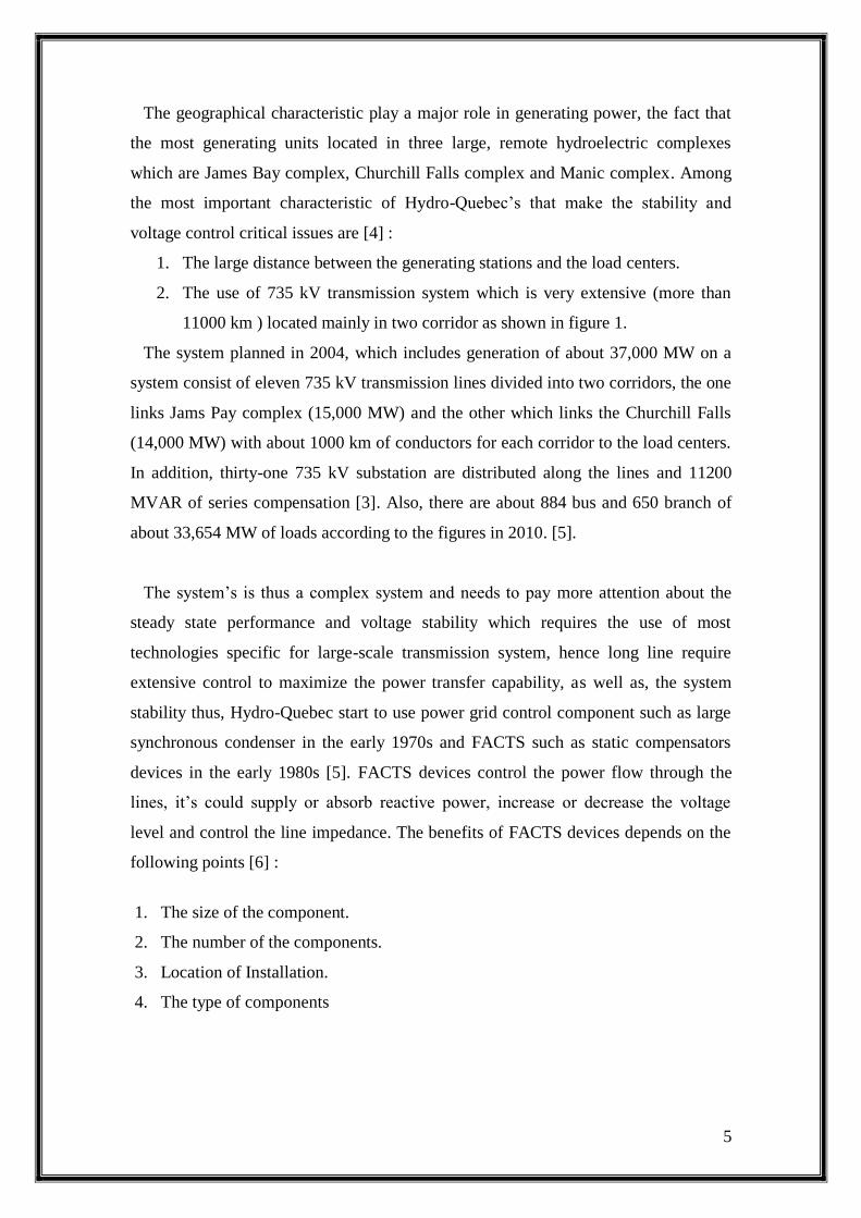
The geographical characteristic play a major role in generating power, the fact that

the most generating units located in three large, remote hydroelectric complexes

which are James Bay complex, Churchill Falls complex and Manic complex. Among

the most important characteristic of Hydro-Quebec’s that make the stability and

voltage control critical issues are [4] :

1. The large distance between the generating stations and the load centers.

2. The use of 735 kV transmission system which is very extensive (more than

11000 km ) located mainly in two corridor as shown in figure 1.

The system planned in 2004, which includes generation of about 37,000 MW on a

system consist of eleven 735 kV transmission lines divided into two corridors, the one

links Jams Pay complex (15,000 MW) and the other which links the Churchill Falls

(14,000 MW) with about 1000 km of conductors for each corridor to the load centers.

In addition, thirty-one 735 kV substation are distributed along the lines and 11200

MVAR of series compensation [3]. Also, there are about 884 bus and 650 branch of

about 33,654 MW of loads according to the figures in 2010. [5].

The system’s is thus a complex system and needs to pay more attention about the

steady state performance and voltage stability which requires the use of most

technologies specific for large-scale transmission system, hence long line require

extensive control to maximize the power transfer capability, as well as, the system

stability thus, Hydro-Quebec start to use power grid control component such as large

synchronous condenser in the early 1970s and FACTS such as static compensators

devices in the early 1980s [5]. FACTS devices control the power flow through the

lines, it’s could supply or absorb reactive power, increase or decrease the voltage

level and control the line impedance. The benefits of FACTS devices depends on the

following points [6] :

1. The size of the component.

2. The number of the components.

3. Location of Installation.

4. The type of components

6

1.2 Transmission system

Transmission system is needed to transmit the power from one location to another

for many reasons, for example, if the natural resources that needed to produce or

generating the power are locating remotely from the consumers, or reduce the number

of the total reserves of the generators. Figure 2 below shows a simplified lossless

transmission system.

Figure 2: Simplified transmission system.

Where:

V1: The sending end voltage.

V2: The receiving end voltage.

ɵ1: The sending end angle.

ɵ2: Receiving end angle.

The line reactance of the line X and the generating power PG.

The power transmitted through the line can be given by equation 1.1 as the following:

The difference in the angle adjusted to match the generated power with the power

required by the load. In case of radial system, the power flow can be determined.

However, in ring configuration, it’s almost impossible to determine the load flow

between two nodes due to variety in loads [1].

1.3 Control of Power Flow in AC systems

One of the important issues regarding the AC transmission system is to control the

power flow, this refers to[7]:

1. Enhance power flow transfer capability.

2. Change power flow under dynamic conditions such as disturbances due to

sudden change in load or line trip (outage) .

3. Insure system stability and steady state operation.

7

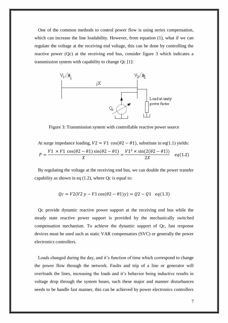
One of the common methods to control power flow is using series compensation,

which can increase the line loadability. However, from equation (1), what if we can

regulate the voltage at the receiving end voltage, this can be done by controlling the

reactive power (Qc) at the receiving end bus, consider figure 3 which indicates a

transmission system with capability to change Qc [1]:

Figure 3: Transmission system with controllable reactive power source

At surge impedance loading, , substitute in eq(1.1) yields:

By regulating the voltage at the receiving end bus, we can double the power transfer

capability as shown in eq (1.2), where Qc is equal to:

Qc provide dynamic reactive power support at the receiving end bus while the

steady state reactive power support is provided by the mechanically switched

compensation mechanism. To achieve the dynamic support of Qc, fast response

devices must be used such as static VAR compensators (SVC) or generally the power

electronics controllers.

Loads changed during the day, and it’s function of time which correspond to change

the power flow through the network. Faults and trip of a line or generator will

overloads the lines, increasing the loads and it’s behavior being inductive results in

voltage drop through the system buses, such these major and manner disturbances

needs to be handle fast manner, this can be achieved by power electronics controllers

8

which have very fast switching characteristic, this will make the AC transmission

system flexible to adapt for changing happened due to load contingencies, load

variety and this lead us to the concept of flexible AC transmission systems (FACTS)

[8].

9

CHAPTER TWO

FACTS DEVICES

2.1 FACTS devices

According to IEEE definition of FACTS: “ Flexible AC transmission systems

incorporating power electronics based and other static controllers to enhance

controllability and increase power transfer capability” [9]. Others define FACTS as :

“power electronics based system and other static equipment that provide control of

one or more AC transmission system parameters” [10].

FACTS devices classified into four categories which are:

1. Shunt connected controllers

2. Series connected controllers.

3. Combined series-series controllers.

4. Combined shunt-series controllers.

Also, depends on the power electronic device used in control process, the FACTS

devices classified also to [11]:

1. Variable impedance type, also called Thyristorvalve.

2. Voltage source converter (VSC) –based.

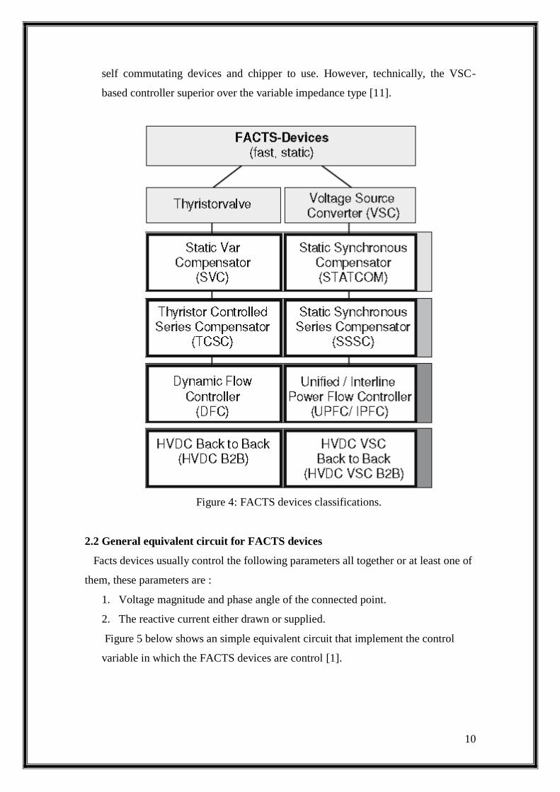
Depending on the connection of the FACT device and it’s control characteristics

or the function to implement, there are many types of these devices according to

the last two categories. Figure 4 below summarize the different types of FACTS

and it’s connection type to the grid.

A small comparison between these two categories, in VSC-based FACTS, they

have compact design, supply the required reactive power (up to a specific limit)

under low voltage levels of the bus and can provide also real power if they have

an energy storage source or large storage DC-link. On the other hand, they needs

an self commutating power semi-conductor devices such as gate turn off (GTO).

For the variable impedance type, Thyristors generally have higher rating than the

10

self commutating devices and chipper to use. However, technically, the VSC-

based controller superior over the variable impedance type [11].

Figure 4: FACTS devices classifications.

2.2 General equivalent circuit for FACTS devices

Facts devices usually control the following parameters all together or at least one of

them, these parameters are :

1. Voltage magnitude and phase angle of the connected point.

2. The reactive current either drawn or supplied.

Figure 5 below shows an simple equivalent circuit that implement the control

variable in which the FACTS devices are control [1].

11

Figure 5: Simplified FACT device equivalent circuit.

Neglecting the losses, ( i) represents drawn or supplied by the FACT device, (e) is

the voltage injected by FACT device respectively .

The following constrain equation (2.1) applied and assuming the pharos

representation of i and e are I and E then:

The current (I) and voltage (E) can be resolved into two components, real (p) and

reactive (r) components in which:

We can represent V1 and I2 as:

Using equation 2.2,2.3 and 2.4 in 2.1 we get:

Positive Vp and Ip indicates real and active power flow, as well as, positive Ir and

Vr indicates positive reactive power that drawn by the FACT device.

The last equations can be considered as general equations for FACTS devices,

hence we will consider the static VAR compensator (SVC), then we can express the

SVC parameters as Vp=0, Vr=0, Ip=0 and Ir= - Bsvc V1, So we can express any

FACT device in term of this parameters. Here in the case of SVC, there are three

constrains and one control variable which is Bsvc.

12

2.3 Static VAR compensator (SVC)

As we mentioned above, SVC classified as variable impedance device, it’s an

umbrella term for several devices, IEEE defines SVC as “ A shunt-connected,

thyristor-controlled inductor whose effective reactance is varied in a continuous

manner by partial-conduction control of the thyristor value”. Figure 6 shown below

gives an illustration about SVC connection through the grid, if the location in the mid

of the line, this have the effect of increasing the maximum power transfer of the line.

However, it’s may located at the end of the line, this have the effect to regulate the

voltage at the end of the transmission line, this analysis is an summary of [1],[13].

Figure 6: SVC connection to transmission system.

Let us perform the analysis at the mid-point of the line, the voltage magnitude at the

mid of the line given by :

Where , B is the propagation constant (rad/m) , w is the angular

frequency, l is the line length and is the power angle.

The system characteristic of the SVC is shown in figure (7-a), points A, B and D

defined the control range of the SVC, the line OA is the SVC in the capacitive region

limits, the line BC region for inductive limits. Vref correspond to reference voltage

when the SVC current ( I) is equal to zero. The SVC current given by:

From figure 7, the slope of the line OA and BC represent the suspetance in

capacitive (Bc) and inductive (BL) region respectively.

13

The SVC voltage can be determined by the intersection between the network

voltage or the network characteristic and the SVC characteristic (control

characteristic), figure (7-b) represent this intersection.

Figure 7-a: SVC Characteristic Figure 7-b: Intersection characteristic

From figure 6 and (7-b), the SVC voltage can be related with the thevenin system

voltage and reactance which is actually the voltage at the SVC or the mid-line and the

reactance’s seen by that SVC, as the following:

Where

and z is the transmission line impedance per km.

And from figure (7-b) and equation (2.6), we can relate Vscv with Isvc graphically

by:

Where Xs or (Bsvc) is the slope of the line AB or OA or BC, depending on the limits.

From equations 2.7 and 2.8, it can be shown that:

Where:

,

,

P0: the power flow of the line without SVC, P1 : is the power flow and the SVC is

included maintain constant voltage at the mid-point.

14

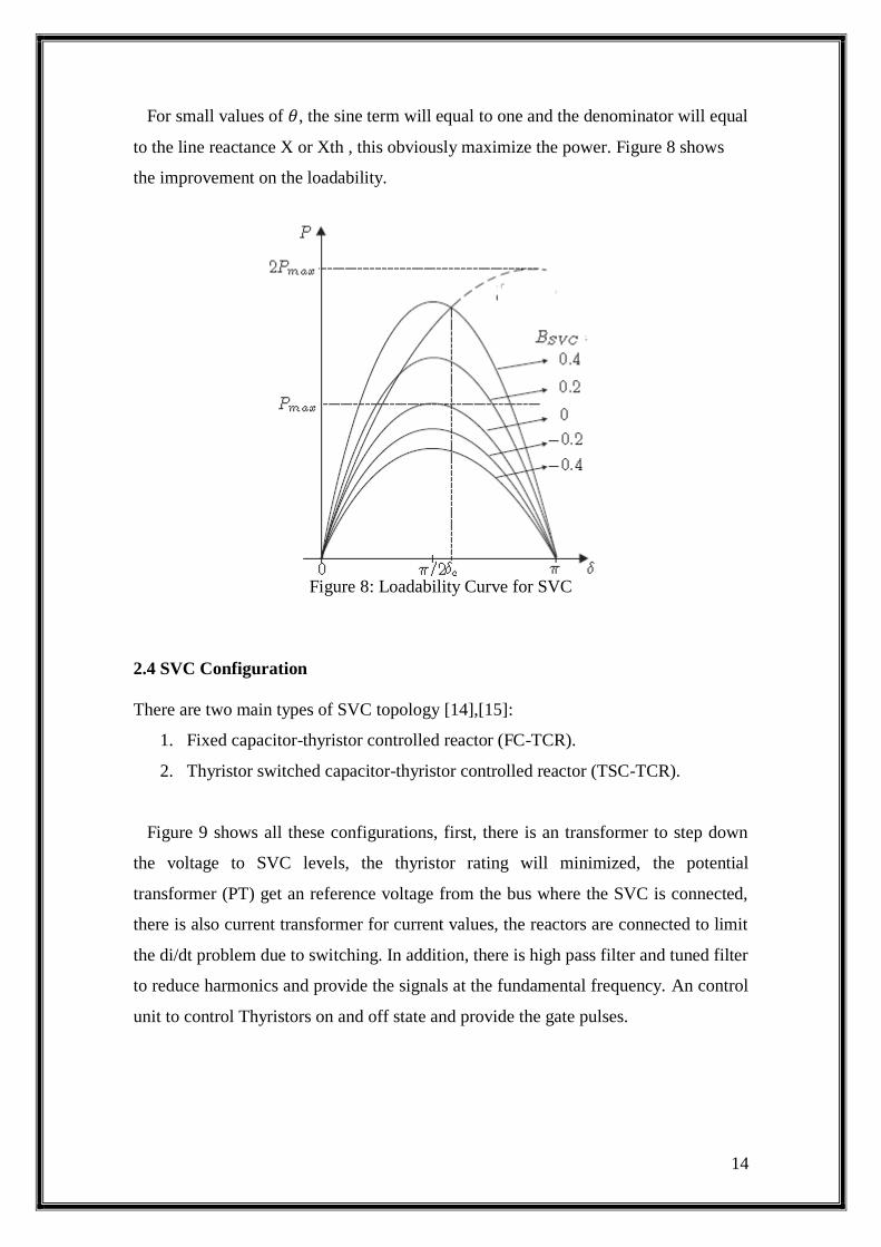
For small values of , the sine term will equal to one and the denominator will equal

to the line reactance X or Xth , this obviously maximize the power. Figure 8 shows

the improvement on the loadability.

Figure 8: Loadability Curve for SVC

2.4 SVC Configuration

There are two main types of SVC topology [14],[15]:

1. Fixed capacitor-thyristor controlled reactor (FC-TCR).

2. Thyristor switched capacitor-thyristor controlled reactor (TSC-TCR).

Figure 9 shows all these configurations, first, there is an transformer to step down

the voltage to SVC levels, the thyristor rating will minimized, the potential

transformer (PT) get an reference voltage from the bus where the SVC is connected,

there is also current transformer for current values, the reactors are connected to limit

the di/dt problem due to switching. In addition, there is high pass filter and tuned filter

to reduce harmonics and provide the signals at the fundamental frequency. An control

unit to control Thyristors on and off state and provide the gate pulses.

15

Figure9: A typical SVC (TSC-TCR) Configuration.

In TCR operation mode, the firing angle ( ) varied from 90o to 180

0 using phase

angle control in which to control the TCR current, figure 10 represent this process.

The same process can be done to TSC, so it’s a matter to control the current flowing

through the elements.

Figure 10: TCR circuit and output wave form.

For switching operation of TSR, the firing angle will be 90 or 180 for full or zero

conduction respectively.

2.5 SVC Controller

SVC controller responsible to provide the firing angle that in turn to control the

current through the TSC and TCR, figure 11 shows a simplified controller operation

to produce the firing angles.

16

Figure 11: SVC Controller.

First, a samples for current and voltage is taken from the potential and current

transformer, an AC filter to prevent parallel resonant, as well as, high pass filter to

prevent low frequency harmonics to pass, the signal then will be rectified and a DC

filter which include low pass filter to remove the ripple from the signal and tuned

filter which is tuned to the harmonics frequencies to prevent it to pass. The auxiliary

signals came from another controllers to obtain full control range, an limiter to

provide the minimum and maximum for the output signal, the logic function will

convert the analog signal to an digital and processed by the CPU to produce the firing

angles [1].

2.6 Benefits of FACTS devices

Some of the benefits that gained from using FACTS devices in our project are:

1. Provide voltage support at critical buses in the system (shunt connected

controllers) which improve the network voltage profile.

2. Improve the line loadability or increase the thermal limit.

3. Overcome dynamic disturbances by fast switching operation.

However, there are some limitations and major issues when applying FACTS

devices in the system, the capital investment which include the instrument cost and

operating cost which represent the power losses on that elements and maintenance.

Also, the payback time. From technical point of view, the location, rating and control

strategy play an important role and used as index for network planning.

17

CHAPTER 3

MODELING AND SIMULATION

3.1 Technical Information and Assumptions

The Hydro-Quebec generating power of about 35,125 MW according to [16]. The

generation stations distribution in MW are shown in table 1.

Table 1: Hydro Generation stations in MW.

The transmission system voltages and substation numbers are shown in table 2, with

total 735/765 kV lines length of more than 10,000 km [16].

Table 2: Transmission system summary.

Hence our goal from this report is to perform the simulation using simulink tool in

Matlab environment. The system that we try to simulate is Quebec international grid.

First of all, many assumptions should be made for simplification, hence Quebec

network is huge complex network, these assumptions as the following:

18

1. Hydro-Quebec network uses 735 kV transmission system, the technical data

for transmission lines, transformers and generators are taken from Matlab

simpower library, actually, this library designed by Hydro-Quebec research

team.

2. The generation units will be designed for JAMES PAY project and

CHURCHILL FALLS project of total power as indicated in figure 1.

3. The system will be designed without any compensation through the lines.

4. The loads are designed in according to the annual report of the company in

2012 [16]. The load bulks will be designed to be in Monterial and Quebec

area.

5. The simulation performed for the network with and without SVC, the

installing location for SVC depends on results founded in [17].

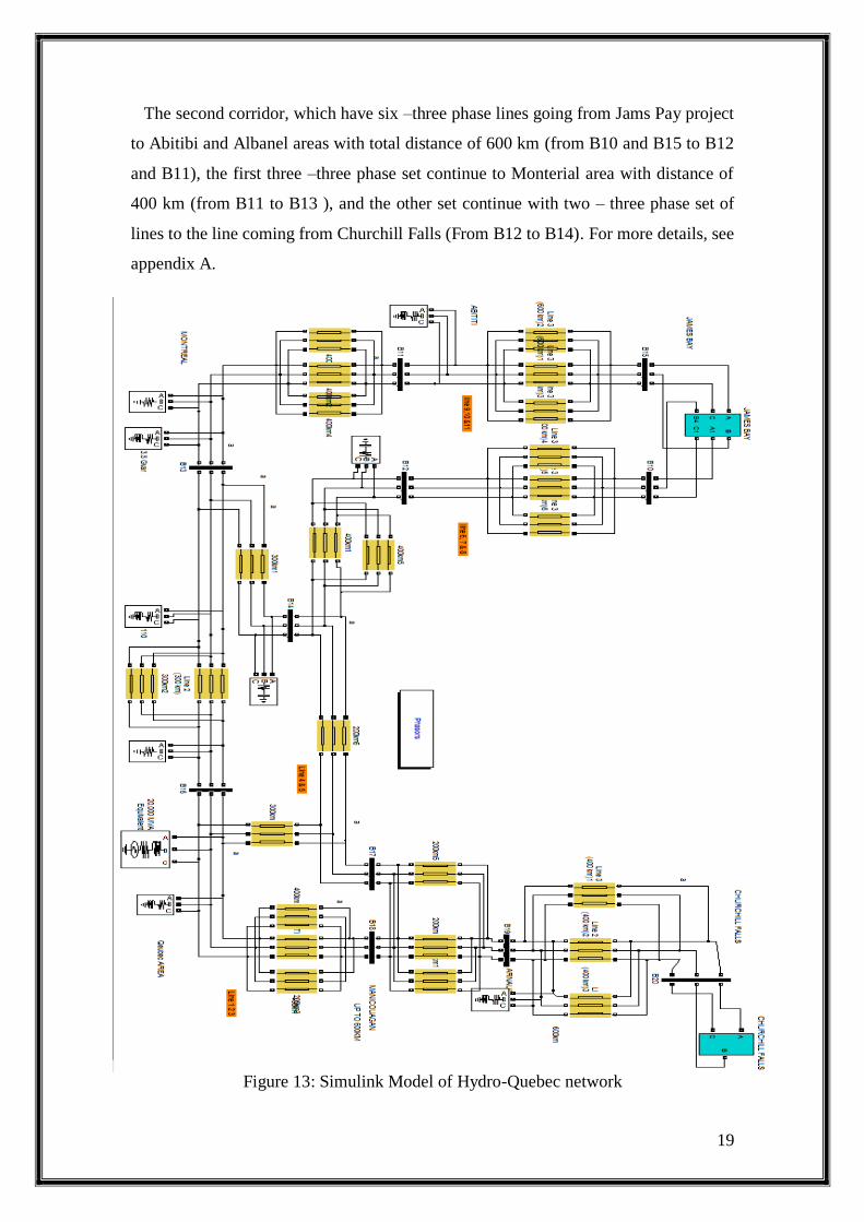
3.2 Simulink Model

The network simulink model is shown in figure 13, notice that there are two

concentrated bulk of power generation units in Jams Pay and Churchill Falls area, the

total power generated is about 17, 000 MW which implement about 50% of the total

power generated in Hydro-Quebec network. The simulink model consist of eleven

735 kV transmission system which is the same as the number of transmission line

physically installed through the network, these lines divided into two corridors, five

lines from Churchill Falls which feeds Quebec area and the around cities in the

southern of the network and connected also to 6 lines came from Jams Pay project

which feeds Montréal and the around cities .

At corridor that links Churchill Falls to the Quebec area, the line divided into three

sub-distances or stages and implement an total length of 1000 km, the first stage

consist of three – three phase, 400 km transmission lines links the stations to Arnaud

area (from B20 to B19), then another two –three phase 200 km transmission lines

links Arnaud to Manicouagan area (from B19 to B18), and continue (with distance of

400 km) to an set of three – three phase lines going from Jams Pay project (from B18

to B16), the third line run to be linked with another three –three phase lines coming

from Jams Pay project with distance of 200 km (from B17 to B16 and B14).

19

The second corridor, which have six –three phase lines going from Jams Pay project

to Abitibi and Albanel areas with total distance of 600 km (from B10 and B15 to B12

and B11), the first three –three phase set continue to Monterial area with distance of

400 km (from B11 to B13 ), and the other set continue with two – three phase set of

lines to the line coming from Churchill Falls (From B12 to B14). For more details, see

appendix A.

Figure 13: Simulink Model of Hydro-Quebec network

20

3.2.1 Transmission lines technical data

The data used for the resistance, inductance and capacitance per kilo-meter are

shown in table 3 below.

Table 3: Transmission line parameters.

Line voltage [kV] Resistance[R1,R0]

[Ohm/km]

Inductance[L1,L0]

[H/km]

Capacitance[C1,C0]

[F/km]

735 [0.01165,0.2676] [0.867e-3,3.0e-3] [13.41e-9,8.57e-9]

From the above table, we can calculate the characteristic impedance, this an very

important quantity to calculate the surge impedance loading (SIL) of the line, which

in turn determine the maximum thermal limit of the line.

From the simulink model initialization, the generators are initiated to generate 1375

MW for each one. The total generation from the northern side is about 17 GW.

Our design consist of 10 lines feeding and extended to 11 , 735 kV as shown in

figure 13.

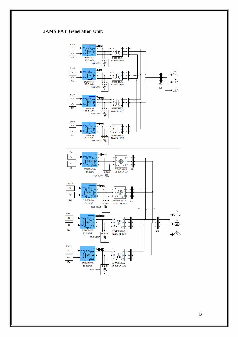
3.2.2 Generation stations and transformers technical data

Each unit consist of an set of synchronous machine models, Jams pay project

produce about 11.5 GW and Churchill Falls produce about 5.6 GW with total power

generated of 17 GW. The generators, as well as, the transformers data are taken from

simpower library in simulink.

21

According to the SIL founded above, this system valid to deliver the required power

by loads. Notice that the system is uncompensated and hence the limits can be

increased by applying the compensation technique to the lines.

3.3 Load distribution

The loads are distributed according to the load centers that usually happened in the

large cites, an large areas such as Quebec and Monteral areas are considered to be the

load centers also, another cities located in the path of the transmission system. The

amount of load values are divided in according to the amount of power generation.

3.4 Simulation results

In this section, the simulation results for voltage profile, as well as, the generated

power will be shown when the system running under normal conditions or unity load

factor , the system is expected to have an good voltage profile which located between

0.95 to 1.05 pu. Then the load factor for the hole loads will increased to 1.09, the

system will be simulated and results for voltage profile and power generation will be

shown. Moreover, the process of adding SVC will be considered at three locations in

the system to improve the system voltage profile, the locations of these SVC’s are

taken from [17]. In addition, we will show that the optimum number of SVCs is three.

With load factor 1, or the loads are about 17 GW, the voltage profile at buses shown

in figure 14:

Figure 14: Voltage profile with unity load factor

22

All busses voltage are within the limits, the minimum bus voltage is 0.953 pu and the

maximum bus voltage is 1.052 pu.

For load factor of 1.09, an increment to the above 17GW loads correspond to 18.53

GW. The voltage profile without installing SVC’s shown in figure 15. (don’t forget

the SIL for lines which is 19.11 GW). The generated power shown in figure 16.

Figure 15: Voltage profile for load factor 1.09 without SVC.

As we can see from figure 15, there are three buses have voltage violation, the first

bus voltage is 1.059 above the maximum allowed voltage, the second has voltage of

0.94 pu, the third has voltage of 0.93 pu below the minimum allowed bus voltage.

Figure 16: Total generated power from P10, P20 and P15.

23

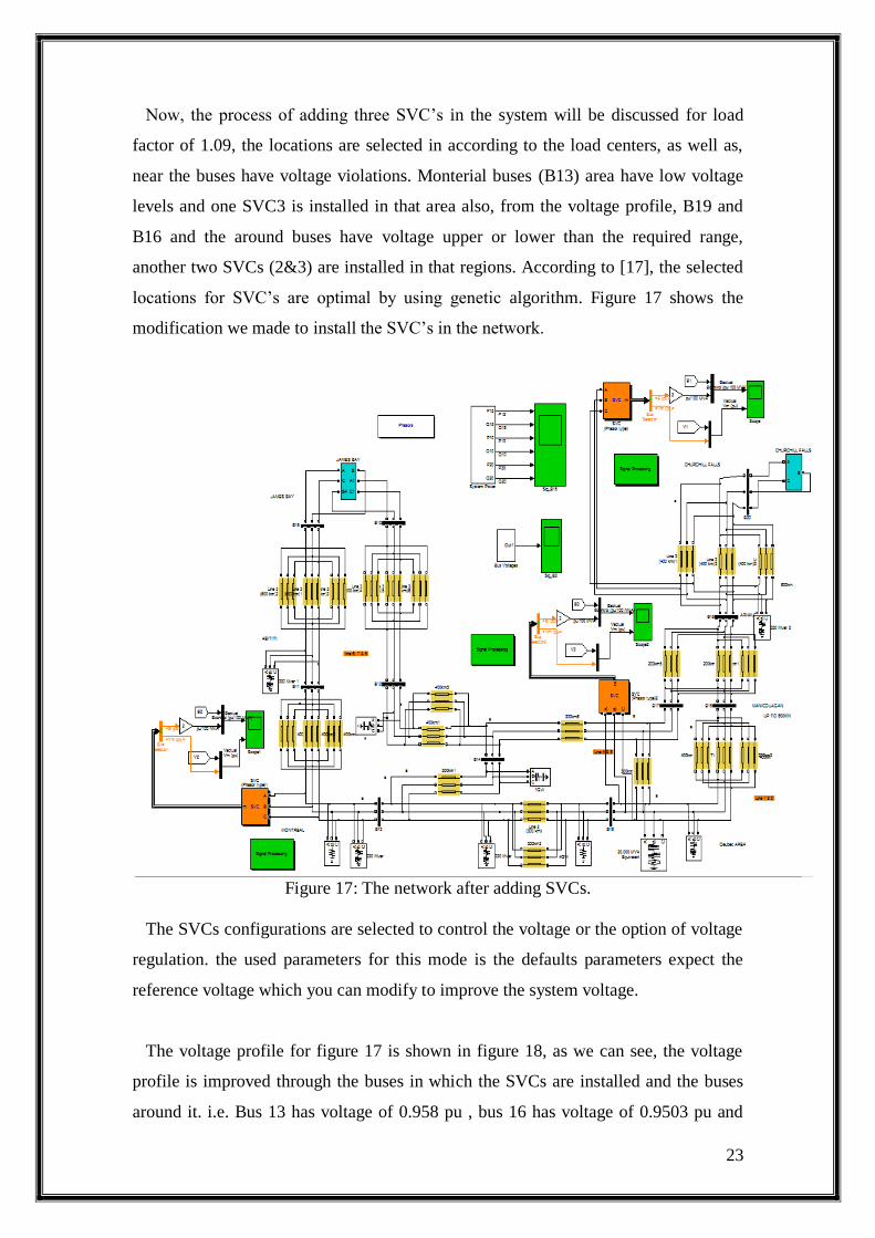
Now, the process of adding three SVC’s in the system will be discussed for load

factor of 1.09, the locations are selected in according to the load centers, as well as,

near the buses have voltage violations. Monterial buses (B13) area have low voltage

levels and one SVC3 is installed in that area also, from the voltage profile, B19 and

B16 and the around buses have voltage upper or lower than the required range,

another two SVCs (2&3) are installed in that regions. According to [17], the selected

locations for SVC’s are optimal by using genetic algorithm. Figure 17 shows the

modification we made to install the SVC’s in the network.

Figure 17: The network after adding SVCs.

The SVCs configurations are selected to control the voltage or the option of voltage

regulation. the used parameters for this mode is the defaults parameters expect the

reference voltage which you can modify to improve the system voltage.

The voltage profile for figure 17 is shown in figure 18, as we can see, the voltage

profile is improved through the buses in which the SVCs are installed and the buses

around it. i.e. Bus 13 has voltage of 0.958 pu , bus 16 has voltage of 0.9503 pu and

24

bus 19 has voltage of 1.048 pu which are improved values for both power increment

and the accepted voltage profile hence the load factor still 1.09.

Figure 18: The voltage profile for load factor 1.09, with SVCs.

The voltage and control characteristics of the SVCs are shown in figure 19,20 and

21. At bus 19, the voltage and control characteristics for SVC-1 is shown in figure 19.

Figure 19: SVC-1 Voltage and control characteristics.

Next, the voltage characteristic for SVC-2 at bus 13 is shown in figure 20.

25

Figure 20: SVC-2 Voltage and control characteristics.

Finally, the voltage characteristic for SVC-3 at bus 16 is shown in figure 21.

Figure 21: SVC-3 Voltage and control characteristics.

Now, we turn to the optimization process, the number of SVC’s will decreased to

two, then it will be increased to four keeping load factor equal to 1.09 for both cases,

also with the same parameters used for the last three locations.

26

1. In case of removing SVC-1 at bus B19, then the system will suffer from

voltage violation at bus 19, actually the voltage at the buses near to B19

increased and a slightly decreasing in other buses occurs. Figure 22 represent

this effect.

Figure 22: Voltage profile after remove SVC-1.

2. Another attempted to remove SVC-2 from the network and return SVC-1 to its

place have worst effect than removing SVC-1, gradual decreasing in the

voltage profile near B19 and the around buses, and heavy decreasing in

voltage at B13 and the around buses, it’s reach 0.93 pu. Figure 23 represents

this effect.

Figure 23: Voltage profile after removing SVC-2.

27

3. Finally, removing SVC-3 from the network and return SVC-1 and 2 to its

original place have also deep effect on the system, the voltage at the buses

near to B19 and the around region decreased from 1.05 to some values near to

1.04 and lower. Also, heavy decreasing in voltage happened at bus B13 and

the near buses which reach 0.93 below the minimum rated value of 0.95 pu.

However, an attempted to increase the number of SVCs in the system have no

significant improvement happened, actually, an fourth SVC added to the system at

different locations other than the current located SVCs and with the same

configuration parameters, the voltage profile slightly decreasing or increasing

depending on the new location of the SVC.

28

Chapter 4

Conclusion and Future Work

This report represented analyses and discussion about the effects of one of the

FACTS devices which is the SVC on the steady state performance regarding the

voltage stability of the Hydro-Quebec Network, three SVCs were installed in the

model, the selected locations are depends on the information provided in [17] hence,

there are two physically installed SVCs in the network in addition to an third one

which added in the simulation environment. Also, the simulation performed to the

system in the steady state operation for unity and with 1.09 increment in load factor in

both with and without SVCs. Based on the results in our model, three SVCs are the

best number of components which can be added to the network, hence our attempts to

increase the number of SVCs for higher than three components in different locations,

almost we get the same result, the voltage slightly decreased or increased depending

on the new installed location. We conclude that three SVCs improve the system

loadability by increasing the load factor from 1 to 1.09 and hence the network still

maintains the voltage profile within the allowed range.

Future Work

From the simulation results in this report, many features can be added to the system

such as:

1. Use a specific algorithm to determine the location of the FACTS devices such

as the Genetic algorithm.

2. Trying to install different types of FACTS devices rather than the SVC.

3. Extend the system to have the series compensation applied in Hydro- Quebec

network .

4. Extend the network to have the third generation station at Manic complex.

Challenging Faced us through our work, the big challenge is ability to perform the

simulation for such huge network like Quebec network, we try our best to make the

system design as the physically installed grid in Quebec. Also, the original system

was designed with another tool rather than Matlab simulink tool.

29

References

1. FACTS CONTROLLERS IN POWER TRANSMISSION AND

DISTRIBUTION, K. R. Padiyar, ISBN (13) : 978-81-224-2541-3

2. http://en.wikipedia.org/wiki/HydroQu%C3%A9bec's_electricity_transmission_sys

tem (Retrieved on 19-12-2014)

3. Discover Hydro-Québec TransÉnergie and its system: Our System at a Glance.

Hydro-Québec TransÉnergie. Retrieve on 15-12-2014.

4. Designing a Reliable Power System: Hydro-Québec’s Integrated Approach,

GILLES TRUDEL, MEMBER, IEEE, JEAN-PIERRE GINGRAS, AND JEAN-

ROBERT PIERRE.

5. Analysing the effects of different types of FACTS devices on the steady-state

performance of the Hydro-Québec network, Esmaeil Ghahremani1, Innocent

Kamwa.

6. Rahimzadeh, S., Tavakoli Bina, M., Viki, A.: ‘Simultaneous application of multi-

type FACTS devices to the restructured environment: achieving both optimal

number and location’, IET Gener. Transm. Distrib., 2009,

7. Power flow control and power flow studies for system with facts devices, Gotham,

D.J. ; State Utility Forecasting Group, Purdue Univ., West Lafayette, IN, USA

; Heydt, G.T., Power Systems, IEEE Transactions on (Volume:13 , Issue: 1 )

8. Utilization Performance based FACTS Devices Installation Strategy for

Transmission Loadability Enhancement ,Ya-Chin Chang ; Dept. of Electr. Eng.,

Cheng Shiu Univ., Kaohsiung, Taiwan ; Rung-Fang Chang, Industrial Electronics

and Applications, 2009. ICIEA 2009. 4th IEEE Conference.

9. N.G. Hingorani, “Flexible AC transmission". IEEE Spectrum, v. 30, 1993.

10. N.G. Hingorani and L Gyugyi, Understanding FACTS – Concepts and

Technology of Flexible AC Transmission Systems, IEEE Press, New York, 2000.

11. Introduction to FACTS Controllers: A Technological Literature Survey,

Bindeshwar Singh, K.S. Verma, Pooja Mishra, Rashi Maheshwari, Utkarsha

Srivastava, and Aanchal Baranwal, International Journal of Automation and

Power Engineering Volume 1 Issue 9, December 2012

12. N.G. Hingorani and L. Gyugyi. Understanding FACTS concepts and technology

of flexible AC transmission systems. IEEE Press, New York, 2000.

13. R.M. Mathur and R.K. Varma. Voltage control and Oscillation Damping. IEEE,

ISSN: 2278-1676 Volume I, Issue 5.

30

14. L. Angquist, B. Lundin and J. Samuelsson, \Power Oscillation Damp- ing Using

Controlled Reactive Power Compensation - A Comparison between Series and

Shunt Approaches", IEEE Trans. on Power Sys-tems, v.8, n.2, 1993, pp.687-700

15. N. Christl, R. Hedin, K. Sadek, P. Lutzelburger, P.E. Krause, S.M. McKenna,

A.H. Montoya and D. Torgerson, \Advanced Series Com- pensation(ASC) with

Thyristor Controlled Impedance", CIGRE , Paper 14/37/38-05, 1992

16. Hydro-Quebec Company annual report 2012.

17. Analysing the effects of different types of FACTS devices on the steady-state

performance of the Hydro-Québec network, Esmaeil Ghahremani1, Innocent

Kamwa.

31

APPENDIX A

Simulink Blocks details

Churchill Falls Generation Unit :

32

JAMS PAY Generation Unit:

33

Power Calculation:

34

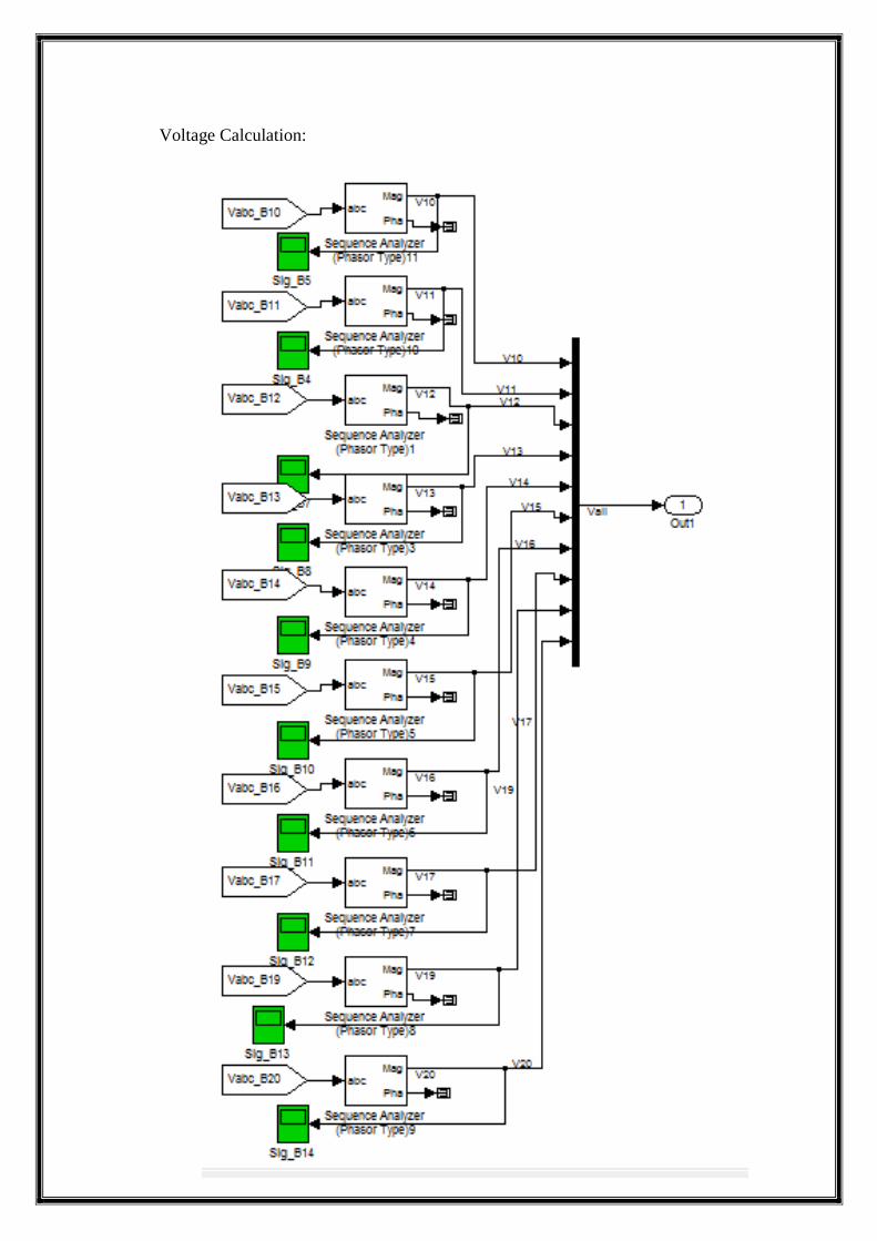
Voltage Calculation: