University of Massachusetts Amherst University of Massachusetts Amherst ScholarWorks@UMass Amherst ScholarWorks@UMass Amherst Masters Theses Dissertations and Theses October 2017 Analyzing Spark Performance on Spot Instances Analyzing Spark Performance on Spot Instances Jiannan Tian University of Massachusetts Amherst Follow this and additional works at: https://scholarworks.umass.edu/masters_theses_2 Part of the Computer and Systems Architecture Commons Recommended Citation Recommended Citation Tian, Jiannan, "Analyzing Spark Performance on Spot Instances" (2017). Masters Theses. 587. https://doi.org/10.7275/10711113 https://scholarworks.umass.edu/masters_theses_2/587 This Open Access Thesis is brought to you for free and open access by the Dissertations and Theses at ScholarWorks@UMass Amherst. It has been accepted for inclusion in Masters Theses by an authorized administrator of ScholarWorks@UMass Amherst. For more information, please contact [email protected].

Welcome message from author
This document is posted to help you gain knowledge. Please leave a comment to let me know what you think about it! Share it to your friends and learn new things together.
Transcript

University of Massachusetts Amherst University of Massachusetts Amherst
ScholarWorksUMass Amherst ScholarWorksUMass Amherst
Masters Theses Dissertations and Theses
October 2017
Analyzing Spark Performance on Spot Instances Analyzing Spark Performance on Spot Instances
Jiannan Tian University of Massachusetts Amherst
Follow this and additional works at httpsscholarworksumassedumasters_theses_2
Part of the Computer and Systems Architecture Commons
Recommended Citation Recommended Citation Tian Jiannan Analyzing Spark Performance on Spot Instances (2017) Masters Theses 587 httpsdoiorg10727510711113 httpsscholarworksumassedumasters_theses_2587
This Open Access Thesis is brought to you for free and open access by the Dissertations and Theses at ScholarWorksUMass Amherst It has been accepted for inclusion in Masters Theses by an authorized administrator of ScholarWorksUMass Amherst For more information please contact scholarworkslibraryumassedu
ANALYZING SPARK PERFORMANCE ON SPOT INSTANCES
A Thesis Presented
by
JIANNAN TIAN
Submitted to the Graduate School of theUniversity of Massachusetts Amherst in partial fulfillment
of the requirements for the degree of
MASTER OF SCIENCE IN ELECTRICAL AND COMPUTER ENGINEERING
September 2017
Department of Electrical and Computer Engineering
ANALYZING SPARK PERFORMANCE ON SPOT INSTANCES
A Thesis Presented
by
JIANNAN TIAN
Approved as to style and content by
David Irwin Chair
Russell Tessier Member
Lixin Gao Member
Christopher V Hollot HeadDepartment of Electrical and Computer Engi-neering
ABSTRACT
ANALYZING SPARK PERFORMANCE ON SPOT INSTANCES
SEPTEMBER 2017
JIANNAN TIAN
BSc DALIAN MARITIME UNIVERSITY CHINA
MSECE UNIVERSITY OF MASSACHUSETTS AMHERST
Directed by Professor David Irwin
Amazon Spot Instances provide inexpensive service for high-performance computing
With spot instances it is possible to get at most 90 off as discount in costs by bidding
spare Amazon Elastic Computer Cloud (Amazon EC2) instances In exchange for low
cost spot instances bring the reduced reliability onto the computing environment be-
cause this kind of instance could be revoked abruptly by the providers due to supply and
demand and higher-priority customers are first served
To achieve high performance on instances with compromised reliability Spark is ap-
plied to run jobs In this thesis a wide set of spark experiments are conducted to study its
performance on spot instances Without stateful replicating Spark suffers from cascad-
ing rollback and is forced to regenerate these states for ad hoc practices repeatedly Such
downside leads to discussion on trade-off between compatible slow checkpointing and
iii
regenerating on rollback and inspires us to apply multiple fault tolerance schemes And
Spark is proven to finish a job only with proper revocation rate To validate and evaluate
our work prototype and simulator are designed and implemented And based on real
history price records we studied how various checkpoint write frequencies and bid level
affect performance In case study experiments show that our presented techniques can
lead to ˜20 shorter completion time and ˜25 lower costs than those cases without such
techniques And compared with running jobs on full-price instance the absolute saving
in costs can be ˜70
iv
TABLE OF CONTENTS
Page
ABSTRACT iii
LIST OF TABLES viii
LIST OF FIGURES ix
CHAPTER
1 INTRODUCTION 1
2 BACKGROUND 5
21 Spot Instance 5
211 Spot Market 6212 Market Volatility 8213 Alternative Service 9
22 Spark the Framework 10
221 In-memory Computing 11222 Resilient Distributed Datasets 12
23 Fault Tolerance 13
231 Recomputing from Lineage 13232 Node Failure Difference 13233 Naıve Fault Tolerance Scheme 14234 Checkpoint 15235 Mixed Fault Tolerance Scheme 15
v
3 RELATED WORKS 16
31 Cloud Computing 1632 Bidding the Cloud 1733 Fault Tolerance 19
4 DESIGN 21
41 Cluster 21
411 Driver Node Life Cycle 21412 Executor Node Life Cycle 21413 Job Classification 22414 Cluster Prototype 23
42 Effectiveness Experiment 24
421 Amplitude 24422 Parallelism Degree 25423 Mean Time to Failrevoke 26424 Mean Time to Write Checkpoint 26
43 Simulator 26
5 IMPLEMENTATION 29
51 Cluster Setup 2952 Simulator Implementation 31
6 EVALUATION 33
61 Evaluation of Effectiveness Experiment 33
611 Base Completion Time 34612 Job Completion in Dynamic Cluster 35
62 Impacts of Parameters 3663 Results from Simulation 38
APPENDICES
A SPOT INSTANCE PRICE RECORDS 42
vi
B SPARK WORKING MODES 45
BIBLIOGRAPHY 46
vii
LIST OF TABLES
Table Page21 Cost-availability trade-off among instance pricing models 622 Mean median spot price and other percentiles in 90 days 723 Comparison of Spot Instance and Preemptible Instance 1041 Factors that potentially affect resilience 2551 Components and compatibility 2952 Control panel 3153 Cluster setting 32A1 east-us-1 On-demand instance pricing 42A2 east-us-1 Spot and Fixed-duration instance pricing 43A3 Market volatility 01 highlighted if 10 revocations per hour 43A4 Market volatility 02 highlighted if 10 revocations per hour 44A5 Baseline job completion time 44A1 Storage level of RDD 45A2 Transformations and actions 45
viii
LIST OF FIGURES
Figure Page21 Price history comparison of m3medium and m3xlarge 922 Market volatility comparison 1023 Spark cluster components 1141 Life cycles of nodes in cluster 2242 Pattern to apply on Spark cluster 2443 Simpler cluster life cycle description 2761 Figure for Table A5 3562 Running time in dynamic cluster 3763 Parameter impacts on job completion time 3864 Verification and extension 3865 Pattern of small drop 1 4066 Pattern of small drop and constant 4067 Price-sensitive pattern 41
ix
CHAPTER 1
INTRODUCTION
Cloud computing has become an overwhelmingly effective solution to build low-cost
scalable online services (Infrastructure as a Service or IaaS) Providers such as AWS Elas-
tic Compute Cloud (AWS EC2) [2] Google Compute Engine [3] and Microsoft Azure [4]
manage large-scale distributed computing infrastructures and rent this compute capac-
ity to customers Compute capacity abstracted from computing resource storage and
network bandwidth etc is rented out as virtual server instance There are situations
when cloud providers have unused active resources and put their idle capacity up at
a cleaning price to maximize revenue Compared to those full-price instances spot in-
stances are much (usually 80) cheaper for compromised reliability [2] In the literature
the terms spot instance transient server preemptible instance have been used interchangeably
to represent virtual server that can be revoked by the provider In this paper we will use
nomenclature spot instance for simplicity Spot instance allows customers to bid at any
expected price [1] The provider sets a dynamic base price according to the supply and
demand of compute capacity and accepts all the bids over the base price On acceptance
customers who bid are granted those instances On the other hand if later the base price
exceeds that userrsquos bid those instances are revoked by the provider
In nature spot instance cannot compete with always-on instance in sense of QoS such
a fact forces customers put non-critical background jobs on spot instances Among multi-
ple QoS metrics particularly availability and revocability are the main concern Availability
1
is defined as the ratio of the total time a functional unit is capable of being used during
a given interval to the length of the interval [18] In comparison revocability indicates
whether a spot instance is revoked under certain circumstance For instance if there are
high-rate price alteration in a short time the high availability can still exist however re-
vocation numbers can be large Moreover revocation can be severe and abrupt in a short
period the amplitude of the price change can be large and the price does not rise grad-
ually And spikes can be extensively observed in figure of price history In our concern
working against revocability of spot instances while most prior work focuses on availabil-
ity as indicated in Section 3
On revocation all the data and application that are deployed on instances are lost
permanently This incurs overhead from not only downtime restart time but time to
recover from loss and rollback as well Therefore job completion time increases when
using spot instances Rising bid effectively decrease the possibility of hitting base price
and hence rate of instance revocation Such a cost-reliability trade-off can lead to some
sophisticated bidding strategy to minimize the total resource cost On the other hand
with software supported fault tolerance schemes the job completion time can also be
minimized
To seek feasibility of complete jobs on spot instances in decent time we deployed
Spark and utilized its fault tolerance mechanism Unlike checkpoint Spark does not re-
cover from disk snapshot by default nor does it recovers from duplicate memory states
that are transferred to other networked machines before failure On submission of appli-
cation Spark yields a list of function calls in order from the program code and hosts it on
the always-on driver node Such a list is called lineage and is used for task scheduling and
progress tracking An implication is that when the current job is interrupted intermediate
states are lost but regenerated in order according to the lineage Such a rollback if there
2
is no other supplementary fault tolerance mechanism in use can hit the very beginning
of the lineage With lineage-based recomputing Spark would handle occasional inter-
ruption well [29] however revocation triggered node failure is much more frequent and
Spark is not specifically designed for such an unreliable computing environment Theo-
retically if rollback to the very beginning occurs can possibly make the job exceed timeout
and never end This brought about the first question that leads to the thesis what is the
impact of node revocation on Spark job completion time and what are factors that affect
performance
To alleviate painful repeated rollbacks we applied compatible checkpoint mechanism
on Spark By default checkpoint is not utilized due to overhead from IO operation be-
tween memory and low-speed disk if there is no interruption routine checkpoint write
does nothing but increase the job completion time However by dumping snapshot onto
disk and later retrieving to the working cluster checkpoint makes it possible that job con-
tinues at the most recently saved state and this would benefit those long jobs even more
Therefore trade-off lies between routine checkpoint write overhead and painful rollback
A question emerges naturally is there optimum that minimizes job completion time
Noticed that the optimization is based on natural occurrence failure that approximately
satisfies Poisson Distribution and it is different from that of market-based revocation So
the question is that whether the mechanism still works on spot market where instances are
bid These questions lead to the thesis Contributions of this thesis are listed below
bull Effectiveness experiment is designed based on prototype Spark program It proves
the effectiveness that Spark cluster can get over frequent revocations We tested
10 20 30 and 60 seconds as mean time between node number alteration (MTBA) and
we found cases with MTBA above 30 seconds can meet time restriction to recover
3
Noticed that this MTBA is much less that price change (not necessarily making node
revoked) from the spot market
bull factors from the cluster configuration and job property are discussed since they may
affect Spark performance They are namely partition number job iteration number
and mean time between node number alteration We figured out that higher parti-
tion degree leads to less processed partition loss and hence shorter recovery time
And as is pointed out shorter MTBA impacts on complete time more And longer
task suffers even more for the recovery process is even longer than those short jobs
bull Mixed fault tolerance scheme is developed and extensively discussed With the inspi-
ration of optimal checkpoint write interval in single-node batch-job case we found
that such optimum is valid for distributed MapReduce job Noticed that in both
cases revocation occurrence satisfies Poisson Distribution In later case studies we
can see that checkpointing with proper optimal interval according to different mar-
ket information can help lower costs when using spot instances
bull Analytic Experiments based on real price history (A collection of example price his-
tory records are hosted on the repository of this project [5]) are conducted To
validate and evaluate our work prototype and simulator are designed and imple-
mented We studied how various checkpoint write frequencies and bid level affect
performance Results from experiments show that our presented techniques can
lead to ˜20 shorter completion time and ˜25 lower costs than those cases with-
out such techniques And compared with running jobs on full-price instance the
absolute saving in costs can be ˜70
4
CHAPTER 2
BACKGROUND
21 Spot Instance
Amazon Elastic Compute Cloud (Amazon EC2) is a web service that provides resiz-
able computing capacity in unit of instance Amazon EC2 provides a wide selection of
instance types to meet different demands There are three basic pricing models for in-
stances from Amazon EC2 Reserved Instance On-demand Instance and Spot Instance
bull Reserved instances allow customers to reserve Amazon EC2 computing capacity for
1 or 3 years in exchange for up to 75 discount compared with On-demand (full-
price) instance pricing
bull On-demand (hereinafter interchangeable with full-price) instance is more flexible
Customers pay for compute capacity by the hour so that they can request instance
when instances are needed
bull Spot instances allow customers to bid on spare compute capacity at discounted
price Customers pay willingly any price per instance hour for instances by specify-
ing a bid
Spot instance can be acquired when there are idle instances from Reserved and On-
demand pools Since the performance of spot instance is equivalent to that of full-price
instance customers can save a lot on performance-thirsty required jobs The provider sets
dynamic spot price for each instance type in different geographical and administrative
5
type Reserved On-demand Spot
price high w discount high lowvolatility NA NA high
availability guaranteed not guaranteed not guaranteedrevocability NA NA when underbid
Table 21 Cost-availability trade-off among instance pricing models
zone Customers bid at desired price for spot instances If a customerrsquos bid is over that
base price the customer acquires the instances On the other hand if later spot price goes
up and exceed the original bid the customerrsquos instances are revoked and permanently ter-
minated In consequence hosted data and deployed applications are lost and job suffers
from rollback If bid is risen customers are more safe to meet less revocations and hence
shorter job completion time We can see that in exchange for low cost the reliability of
spot instances is not guaranteed Table 21 shows comparison of instance pricing models
211 Spot Market
Spot market is a fair market where the provider and customers mutually agree on
the service price above an base price The base price fluctuates according to supply and
demand Spot price ranges from 01x to 10x full price of the same instance type On rare
occasions although it goes over 10x full price it is far below 10x on average Despite
of the average low price the price change can be severe price change abruptly to a high
level and fall to a rather low level in a short period (short enough so that a job cannot even
be finished)
Table A1 in Appendix shows pricing for On-demand (full-price) instance in east-us-1
as of year 2014 and Table A2 in Appendix chapter shows pricing for newly released fixed-
duration as complementary pricing model
6
types mean 3rd 5th 10th 25th median 75th 90th 95th 97th
c3
large 0179 0159 0160 0161 0165 0170 0176 0187 0198 0210xlarge 0207 0165 0167 0170 0177 0191 0214 0252 0292 0329
2xlarge 0232 0181 0184 0189 0202 0221 0250 0287 0312 03394xlarge 0251 0168 0172 0178 0191 0214 0254 0327 0417 04988xlarge 0215 0162 0163 0166 0172 0185 0208 0247 0281 0326
d2
xlarge 0172 0103 0103 0103 0106 0160 0205 0259 0305 03412xlarge 0130 0105 0106 0107 0112 0121 0132 0145 0173 02054xlarge 0126 0103 0103 0104 0105 0109 0122 0156 0194 02268xlarge 0122 0102 0102 0103 0104 0108 0129 0145 0173 0181
g2 2xlarge 0197 0126 0129 0134 0148 0175 0215 0267 0307 03538xlarge 0355 0151 0160 0174 0201 0269 0385 0651 1000 1000
i2
xlarge 0123 0100 0101 0101 0104 0115 0140 0152 0160 01672xlarge 0125 0103 0103 0104 0108 0118 0133 0148 0159 01694xlarge 0139 0103 0104 0104 0106 0115 0147 0185 0205 02188xlarge 0122 0101 0101 0102 0103 0107 0129 0156 0161 0169
m3
medium 0156 0131 0131 0134 0139 0148 0169 0185 0200 0210xlarge 0164 0138 0140 0144 0151 0161 0172 0185 0196 0206
2xlarge 0170 0139 0141 0145 0154 0166 0180 0198 0212 0224large 0151 0132 0133 0135 0138 0144 0154 0175 0199 0218
r3
large 0129 0100 0101 0102 0106 0114 0128 0150 0179 0210xlarge 0186 0104 0106 0112 0126 0147 0191 0284 0379 0474
2xlarge 0168 0111 0114 0119 0131 0151 0183 0227 0268 03034xlarge 0145 0099 0100 0102 0107 0117 0140 0192 0267 03448xlarge 0165 0112 0114 0119 0130 0151 0181 0218 0256 0288
Table 22 Mean median spot price and other percentiles in 90 days
7
212 Market Volatility
Same-type instances are priced approximately the same across different geographical
regions Here we take us-east-1 as example to analyze on spot market volatility in the
Unites States
Instances are differentiated by purpose eg general-purpose memory-optimized for
intensive in-memory computing and GPU-optimized for graph algorithms and machine
learning For full-price instances all same-purpose instances are price the same for unit
performance A unit performance is defined by price per EC2 Compute Unit (ECU) and
it can be represented alternatively as ratio of spot price to full price So we adopted this
ratio as standardized price to measure the spot price as illustrated in Equation 21
ratio =spot price
on-demand price=
spot priceECU numberOD priceECU number
=spot price per ECUOD price per ECU
(21)
where full-price is fixed for each type
Due to supply and demand the ratio for same-purpose instance can be different An
example of comparison between m3medium and m3xlarge is shown in Figure 21 On
bidding strategies we may bid for several small instances or a single large instance deliv-
ering the same performance Which to bid may depend on the granularity to which a job
is partitioned And it is related to Section 32 This brings forth a critical question high
revocation rate causes cascading node failure and data loss is it even feasible to deploy
application even with abundant fault-tolerant mechanisms This leads to observation on
volatility of the market Although this can lead to a sophisticated bidding strategies in
this paper we are not going to discuss further on this
We also gave a general comparison among all instance types in Figure 22 In spot
market bidding level determines availability To give an intuitive view over availability
we supposed in the past three months we bid for each type of instance at exactly the mean
8
Figure 21 Price history comparison of m3medium and m3xlarge
price and count revocation number thus revocation rate due to underbids can reflect the
spot market volatility We defined revocation rate as revocation number per 24 hours
(only records in most recent three months can be retrieved from official source however
3rd-party communities maintain much longer history)
Figure 22 shows widely distributed bid-revocation information In this Figure X-axis
is given by mean spot price during 90 days (in this project it is March 13 to June 13 2016)
and the data is standardized as ratio of spot price to full-price Y-axis is given by mean
revocation number every 24 hours when bid level is set to the aforementioned mean price
As we can see most instance types (g28xlarge type is the only exception in this study)
are lowly priced but revocation rates are widely distributed We can take c32xlarge
c34xlarge g22xlarge and c3large as examples
213 Alternative Service
Preemptible instance from Google Compute Engine (GCE) is an alternative option of the
spot instances Customers also create and run virtual machines on its infrastructure [3]
GCE might terminate (preempt) these instances if it requires access to those resources for
other tasks although pricing is not auction based (fixed instead) Additionally Compute
Engine has a finite number of available preemptible instances so customer might not be
9
00 02 04 06 08 10
Mean spot price divided by same-type on-demand price
0
200
400
600
800
1000
1200
1400
1600
Mea
nre
voca
tion
num
ber
ever
y24
hour
s
g28xlargehigh mean pricelow volatility
g22xlargelow mean pricelow-medium volatility
c34xlargelow mean pricemedium-high volatility
c32xlargelow mean pricehigh volatility
c3largelow mean pricelow volatility
Market Volatility Measuringc32xlarge
c34xlarge
c38xlarge
c3large
c3xlarge
d22xlarge
d24xlarge
d28xlarge
d2xlarge
g22xlarge
g28xlarge
i22xlarge
i24xlarge
i28xlarge
i2xlarge
m32xlarge
m3large
m3medium
m3xlarge
r32xlarge
r34xlarge
r38xlarge
r3large
r3xlarge
type mean revocprice rate
c3large 0215 481c3xlarge 0220 8452
c32xlarge 0240 14965c34xlarge 0257 9079c38xlarge 0215 6568d2xlarge 0191 1116
d22xlarge 0151 510d24xlarge 0170 529d28xlarge 0160 281g22xlarge 0248 4831g28xlarge 0679 862
i2xlarge 0123 2671i22xlarge 0126 4030i24xlarge 0148 1927i28xlarge 0125 1081
m3medium 0199 333m3large 0169 1745
m3xlarge 0173 10398m32xlarge 0183 9563
r3large 0130 1915r3xlarge 0204 7390
r32xlarge 0169 14185r34xlarge 0162 6167r38xlarge 0178 8885
Figure 22 Market volatility comparison
able to create them during peak usage [15] Comparison of AWS Spot Instance and GCE
preemptible instance is listed in Table 23
provider AWS Spot Instance Preemptible Instance
pricing fluctuating bidding required fixedcondition of yielding bidding failure preempted by higher high-priority taskson yielding instance terminated (same) instance terminated
Table 23 Comparison of Spot Instance and Preemptible Instance
22 Spark the Framework
Apache Spark is a general-purpose parallel-compute framework that supports exten-
sive data processing primitives Spark Core a collection of core functionality drives high-
level applications There is an optimized engine that supports general execution graphs
10
Spark SQL for SQL and structured data processing MLib for machine learning GraphX for
graph processing and Spark Streaming Spark structure is shown in Figure 23
Apps
SparkSQL
SparkStreaming
MLib(machine learning)
GraphX(graph)
Spark Core
HDFS S3
Mesos Hadoop YARN
Infrastructure
Access and Interfaces
In-house Apps
ProcessingEngine
Storage
ResourceVirtualization
Hardware
Figure 23 Spark cluster components
In this paper we focus on designing programs with primitives from Spark Core These
primitives are classified into two categories transformation and action A complete list of
transformation and action is shown in Table A2
221 In-memory Computing
Traditional Hadoop Distributed File System (HDFS) is an abstract distributed file system
primarily for managing data Although HDFS is primarily for Hadoop application it
is ubiquitously used by distributed frameworks Due to the fact that for read operation
is much frequent than write operation it is designed write-once-many-access feature for
simple coherence and derived intermediate states are written back to disk For those
applications that mainly work over data access rather than data write HDFS contributes
high throughput however it is against the nature of those applications that generate vast
of intermediate results Particularly when it comes to iterative tasks it incurs severe
overhead of swapping transient states out and in to low-speed storage thus it deteriorates
the overall performance
11
Spark incorporates popular MapReduce methodology Compared with traditional
Hadoop MapReduce Spark does not write intermediate results back to low-speed disk
Instead Spark maintains all necessary data and volatile states in memory
222 Resilient Distributed Datasets
Resilient Distributed Datasets (RDD) is the keystone data structure of Spark Partitions
on Spark are represented as RDD By default necessary datasets and intermediate states
are kept in memory for repeated usage in later stages of the job (Under rare circumstance
with insufficient physically memory in-memory states are swapped out onto low-speed
disk resulting in severely downgraded performance) RDDs can be programmed per-
sistent for reuse explicitly such an operation is materialization otherwise RDDs are left
ephemeral for one-time use
On job submission to Spark the program code is unwound and recorded as a list
of procedural function calls terminologically lineage On execution lineage is split into
stages A stage can start with either a transformation or an action A transformation liter-
ally transform a type of data hosted in RDD into another type in RDD while an action in
the end output data in regular types that are not used for in-memory computing With
syntactical support of lazy evaluation Spark starts executing transformation operations
only when the program interpreter hits action after those transformations Such a scheme
is used for scheduling and fault tolerance (see details in Section 23) Scala programming
language [14] is used to call function in Spark program
12
23 Fault Tolerance
231 Recomputing from Lineage
Consistent with in-memory computing fault tolerance is accomplished by utilizing
lineage as preferred To simplify question Spark driver program is hosted on supposedly
always-on instance Thus lineage generated in driver program is never lost and fault
tolerance system can fully work towards recovery
On node failure volatile states in memory are lost Rather than recover from du-
plicate hosted on other machine before failure this part of lost node can be computed
from other states specifically it can be generated from original datasets With progress
tracked in lineage recovery can start from the very beginning of the lineage and finally
reaches the failure point Programmatically Spark supports recomputing from lineage
and checkpoint mechanism And these are discussed in Section 233 and 234 Multiple
fault tolerance mechanisms and schemes are also compared in Section 33
232 Node Failure Difference
There are several differences lying between natural node failure in datacenter and
revocation triggered failure
bull in industry mean time to fail (MTTF) are used measure failure interval in unit of
hundreds of days which is much longer ( 10000x) than interval for a price change
thus potential revocation
bull natural node failure occurrence obeys non-memorizing distribution In the single-
node case Poisson Distribution is reasonable approximation However there is no
evidence showing that revocation triggered node failure obey such distribution
bull Spot prices fit in to Pareto and exponential distributions well [32] while revocation
distribution is more complex for different bidding schemes
13
Some sophisticated bidding strategies [32 23] are derived While some argued there is
no need to bid the cloud [24 26] for different reason (see details in Section 32) We focus
on invariant in running Spark job on spot instances no matter how we bid the cloud
233 Naıve Fault Tolerance Scheme
Recomputing from lineage makes it possible to recover from failure without external
backups However the effectiveness of the exploiting recomputing scheme is undeter-
mined There are some positive factors from the cluster configuration that help recover
bull data storage and application are deployed differently Data is hosted on HDFS clus-
ter other than the compute cluster or hosted in S3 bucket
bull it is inexpensive and preferred to deploy driver program on a single always-on node
to avoid lineage loss
More related cluster configuration is listed in Section 41
However there many negative factors that undermines the recovery severely
bull Revocation is much more frequent than natural node failure in datacenter and
bull Despite the strong resilience of Spark (recovering when there is only small number
of nodes in the cluster) revocations in sequence applies cascading state losses on
the cluster making it even harder to recover
A fault tolerance scheme is application with specified parameter of its cornerstone
mechanism Compared to natural node failure this fault tolerance mechanism is not de-
signed for high failure rate It is highly possible to exceed system-specified timeout and
the job is terminated This leads to a later effectiveness experiment stated in Section 42
As we pointed out later although it is not guaranteed to complete job without exceeding
timeout we can cut off those timeout tasks by configuring mean time between failure
14
234 Checkpoint
Compatible checkpoint write is disabled in Spark by default for performance consid-
eration This supplemental mechanism can be enabled both in program code and configu-
ration Technically RDD can be differentiated by storage level (see details in Table A1) By
default MEMORY ONLY is preferred to use to achieve better performance Flexible on-disk
materialization for specific RDDs can be done by programming rather than hard-setting
ON-DISK for all RDDs On job failure disk-cached states will be immediately ready after
loading This alleviate cascading rollbacks and recompute from beginning However if
there is no failure routine checkpoint write is wasteful only to extend job completion
time This motivate us to utilize mixed fault tolerance scheme
235 Mixed Fault Tolerance Scheme
As discussed earlier we can balance overhead of routine disk write and rollback This
arise the second question what the optimum of checkpoint write interval is if any In-
spired by single-node batch-job case we applied a first-order approximation on finding
optimum of checkpoint write interval to minimize the total job completion time The
evaluation is shown in Chapter 6
15
CHAPTER 3
RELATED WORKS
This thesis focuses on analyzing the performance and cost of running distributed data-
intensive workloads such as Spark jobs on transient servers such as AWS Spot Instances
and GCE Preemptible Instances Below put our work in the context of prior work that has
examined a variety of bidding strategies and fault-tolerance mechanisms for optimizing
the cost and performance on such transient servers
31 Cloud Computing
There are several topics related to cloud computing infrastructure
bull In-memory computing Data reuse is common in many iterative machine learning and
data mining [29] Pessimistically the only way to reuse before computations is to
write it to external stable storage system eg HDFS [8] Specialized frameworks
such as Pregel [21] for iterative graph computations and HaLoop [9] for iterative
MapReduce have been developed However these frameworks support limited
computation patterns In contrast Spark is general-purposed and offers primitives
for data processing The abstraction for data reuse as well as fault tolerance is (RDD)
Materialization can be toggled by programming in sense of data reuse with the sup-
port of RDDs In the programmed application a series of data processing procedure
along with explicit materialization of intermediate data is logged as lineage Such a
setting lead to quick recovery and does not require costly replication [29]
16
bull Multi-level storage Although materialization of reused data boosts performance node
loss annihilates such efforts and makes it useless on high-volatile cluster In our
work we took a step back We took advantage of multiple storage level (see Ta-
ble A1) not only low latency in the process but the global minimizing completion
time is the goal To resolve such issue we employ checkpointing along with built-in
recovery form other RDDs Despite the fact that overhead from disk-memory swap-
ping is introduced again we leverage its short recovery and avoidance of recompute
from very early stage of a logged lineage
bull Practice In-memory computing requires abundant memory capacity in total Spark
official claimed that the framework is not as memory-hungry as it sounds and the
needed original datasets are not necessary to loaded into memory instantly in ad-
dition multiple storage level including memory andor disk and the mixed use
of them can be configured to resolved the issue of materialization required capac-
ity [6] It could be true if base memory capacity is satisfied when the cluster node
availability is stable however when node availability is low performance suffers
from both the limited memory capacity and memory state loss such that swapping
in and out happens frequently and thus latency becomes much more serious Such
overhead is also discussed in Chapter 6
32 Bidding the Cloud
Spot price alteration reflects and regulates supply and demand This is proven and
discussed further in [10] for the provider it is necessary to reach market equilibrium
such that QoS-based resource allocation can be accomplished
bull Strategic bidding Zheng et al [32] studied pricing principles as a critical prerequisite
to derive bidding strategies and fit the possibility density function of spot price of
17
some main types by assuming Pareto and exponential distributions Such fitting
helps predict future spot prices He et al [16] implemented a scheduler for bidding
and migrate states between spot instances and always-on on-demand instances
Analysis in [22] shows the sensitivity of price change a small increase (within a spe-
cific range) in bid can lead to significant increment in performance and decrement
in cost Though the sensitivity to price is also observed in our experiment (as shown
in Chapter 6) it is more than aforementioned reason 1) qualitative change occurs
when bid is slightly increased to the degree where it is above price in most of time
And scarcely can revocation impact on performance and thus total cost instead the
dominating overhead is from routine checkpoint write to disk 2) on the other hand
when bid is not increased high enough to omit most of revocations a dramatically
high performance is accomplished by much less rollback when checkpointed at ap-
propriate frequency
bull Not bidding Some argued not biding is better without knowing the market operating
mechanisms deeply Not developing bidding strategies can be attributed to several
reasons 1) Technically IaaS providers can settle problem of real-time response to
market demand [33] and short-term prediction is hard to achieve 2) customers can
always find alternative instances within expected budget [24] for market is large
enough 2) there are abundant techniques that [25 24] ensure state migration within
the time limit and 3) some pessimistically deemed that it is not even effective to bid
the cloud since cascading rollbacks caused by revocation is so painful to recover
from and framework improvement is the key point to solution [26]
18
33 Fault Tolerance
Bidding strategy is helpful and we need specified bidding schemes to conduct experi-
ments and to compensate less effective bidding strategies we fully utilized fault tolerance
mechanisms to archive equivalent effectiveness And despite of intention of not bidding
the cloud we set different bid levels for 1) it is related performance and sometime per-
formance is sensitive to the corresponding availability and 2) data-intensive MapReduce
batch jobs has been studied in [20 16 11] Our part of job is not the traditional MapRe-
duce with static original datasets that is pre-fetched and processed rather some job does
not really rely on old intermediate states ie streaming although QoS is not guaranteed
Most of the prior work focuses on improving availability and thus QoS by develop-
ing bidding strategies Nevertheless higher availability does not necessarily result in
low revocation rate Yet Spark is employed to process data-intensive jobs high-rate price
alteration may lead to high revocation rate There are several main fault-tolerance ap-
proaches to minimize impact of revocations (ie intermediate state loss and progress
rollback) checkpointing memory state migration and duplicate and recomputing from
original datasets
bull Live migrationduplication Prior work of migration approaches is presented in [24 25]
And fast restoration of memory image is studied in [31 19] In contrast our origin
working dataset is hosted on always-on storage while intermediate is mostly gener-
ated online for ad hoc practices expect the checkpointed portion to avoid overhead
from network [30] And these static integrity ie integrity is ensured due to com-
plete duplication differs from freshly regenerated intermediate states Such differ-
ence lead to our investigation on more than checkpointing schemes
19
bull Fault tolerance schemes Checkpointing for batch jobs [12 13] and its application on
spot instances [27] are studied We adopt the origin scheme into distributed case
and mixed use of both checkpoint read and regeneration
[28] gives four basic and various derived checkpointing schemes with mean price
bidding In our work mean price bidding is only used for illustrating market volatil-
ity(see Section 212) yet mean price bidding is not key to optimize Listed basic
checkpointing schemes includes hour-boundary rising edge-driven and adaptively
deciding checkpointing Results from [28] shows empirical comparison among cost-
aware schemes however 1) before extensive discussion on other three basic meth-
ods hour-boundary checkpointing can still be deeply investigated by changing check-
point write interval and 2) for different bidding-running cases the optimal check-
point write interval can be different which implies routing checkpoint write of
variable interval can be employed such a method along with its derived variable-
interval checkpoint write can be effective while maintaining its simplicity
In addition compared to [20 16 11] where given grace period of 2 minutes is used
for live migration in our case the grace period is mainly used to finish writing
checkpoint to external HDFS (Otherwise even the next stage can be finished it is
lost in the next moment)
20
CHAPTER 4
DESIGN
41 Cluster
Suppose we choose a cluster of nodes from a node pool And this cluster comprises a
single master node (driver node) and multiple slave nodes (executor nodes) Via control
panel we can control over the cluster in the remote datacenter Noticed that a node reg-
istered under a framework can be easily replaced since compute capacity is ubiquitously
multiplexed and we can always migrate workload from one to another [17] Before we
run Spark jobs on instances and recover job from failure we first figured out how driver
and executor nodes work in the cluster
411 Driver Node Life Cycle
Driver node goes with the cluster until the cluster is terminated or expires The driver
node handles 1) partition designation as well as balance workload throughout the cluster
2) catching exceptions catch 3) recovering from node failure 4) issuing checkpoint write if
appropriate and 5) synchronizing progress through all the executor nodes Spark driver
node life cycle is depicted in Figure 41
412 Executor Node Life Cycle
As we can see after acquiring the executor node once its bidding is over the threshold
price set by the service provider After being acquired executor node is under control
of driver node and is to be designated workloads If there is no interruption caused by
21
underbid the node runs and finally exits peacefully otherwise it is terminated and its
alternative is requested to the cluster Executor node life cycle is depicted in Figure 41
Driver node life cycle
Executor node life cycle
ready processing finished
ldquoterminatedrdquo
check bid sync-ed
bid lt spot price
bid gt spot pricerequested
on-node partitions gone
through the entire lineage
master signaling
bid lt spot
price
master syncack
(interruptio
n)
(time R) (designed to node)
exit
(stage+1)
ready designate all partitions paused finishedsync-ed
checkpoint write
designate most lagging partitions
executors computing
exception handling
all eligibly-on nodes sending
syncreq
gone through the entire lineage
checkpoint disabled
initializedall executor
designed partitions
checkpoint enabledcheckpoint write finished
exciting stragglernot exciting
(time δ)
exit
(stage+1)
(stage+1)
interruption
ldquo(ltevent-namegt)rdquo indicates time elapsed or event emerging during the state transactionldquolttransaction-conditiongtrdquo indicates transaction condition from one state to another
Presumedly interruption occurs only when executor node runs into ldquoready and computingrdquo phase And presumedly we donrsquot bid for more nodes whose total number exceeds the original setting
Figure 41 Life cycles of nodes in cluster
413 Job Classification
Real-world jobs can be roughly classified into two categories
1 Iterative MapReduce application as an example is one kind when executed on
Spark cluster stages are inter-dependent since input for a stage is always the out-
put from previous stage Obviously in such cases the all the intermediate and final
results can be attributed to the first stage and the very input datasets In this way
if a revocation occurs all the active nodes are paused until the lost intermediate are
generated from the very beginning
22
2 Unlike stage-interdependent tasks when the node number decreases there is no
need to start over rather old lost RDDs is simply not needed any more instead the
processing capacity shrinks A good example would be streaming although there
is no iteration that forms a stage streaming often comes with data retrieving and
analyzing online which could be coded into transformations and actions
414 Cluster Prototype
We built a prototype dynamic cluster whose node number always changes A specific
number of full-price (always-on) instances to ensure full control over the node availabil-
ity Cluster can be manipulated via control panel such that Spark executor processes are
manually terminated and restarted on need basis Such a design simulates node loss and
new node requests in the spot market
Suppose Spark runs under periodic pattern of fluctuating node availability And such
a given pattern is discretized to fit in to integer node number (see Figure 42) Thus
job completion time in such a dynamic cluster can be observed and compared to that
in static cluster with no node number change The sample rate determines mean time be-
tween mandatory pattern alteration and the interval is defined as a unit time Noticed that
in a periodic pattern there are two phases 1) on ascending phase new nodes are added
and 2) on descending phase nodes are revoked So shrinking MTBA can either boost
computing (on ascending phase) or deteriorate node loss even more and vice versa In
later results (see Section 62) we can see that MTBA is key parameter and may determine
whether Spark can survive cascadingconsecutive revocations or not
23
0 20 40 60 80 100
Time (unit)
0
5
10
15
20
Exe
cuto
rN
ode
Num
ber
(uni
t)Ideal Cosine Pattern
Pattern
Mean Node Number
0 20 40 60 80 100
Time (unit)
0
5
10
15
20
Exe
cuto
rN
ode
Num
ber
(uni
t)
Discrete PatternDiscrete Pattern
Mean Node Number
Figure 42 Pattern to apply on Spark cluster
42 Effectiveness Experiment
We conduct experiments to prove that it is possible to run Spark job in decent time with
proper parameters Noticed that number of data partitions or RDD are constant from the
view of the system rather than in a queue to be designated on new nodes these RDDs
are crammed on existing active nodes For discussing effectiveness and more details
the amplitude cached RDD number and mean time to fail are manipulated We hard-
set some factors to reasonably simplify the problem (see Table 41) And we conduct
experiments over parameters that listed below
421 Amplitude
Amplitude of pattern is a direct parameter that impacts We first set a (10plusmn 6)-node
dynamic cluster which in long term average node number is 10 A stage holds 0+ trans-
formation and 1+ action calls recall that lazy evaluation lying in the scheduling basis and
RDD if lost is regenerated from the lineage back to a specific stage (need action to trig-
ger) Thus with the cached and to-be-regenerated RDD number constant theoretically
if the job recoverable a stage with less active executor node would run for long time to
finish this stage To exemplify the varying situation we first set a (10plusmn 4)-node dynamic
cluster whose mean node number in long term is the same with a 10-node static cluster
24
parameters how it affects
performance instatic cluster
Performance in the static cluster outlines the best performancethat can be possibly achieved in the dynamic cluster In the dy-namic cluster if there is no node failure and thus rollback jobcompletion by stage whose time determined by the performancein the static cluster would not be repeated So avoiding revocationas much as possible lead to optimal results
timeout Timeout is criterion for the system to terminate the job and timelimit within which node connectivity issues must be resolved Bydefault after three attempts on reconnection with the failed nodethe current job will be killed by driver program
CPU core More available CPU cores are almost positive for everythingIn our experiment we restricted CPU core per node (usingm3medium instances)
checkpointwrite
Checkpointed job does not need to start over However if there isno failure checkpoint write time is wasteful In the effectivenessexperiment to test if Spark without high-latency checkpointingcan complete jobs
Table 41 Factors that potentially affect resilience
without node loss and addition Later a change in amplitude are discussed Results of
these sub-experiments are stated in Chapter 6
422 Parallelism Degree
Cached RDD number (or parallelism degree) in total is set to 20 making maximum of
hosted RDD number on each executor node less than 20 By default an equivalent CPU
core can process 2 RDDs at the same time thus as active node decreases average number
of RDD hosted on executor node exceeds 20 and simply lengthen job completion time
for this stage by at least 100 There is also an auxiliary experiment to see how RDD per
node impacts performance
25
423 Mean Time to Failrevoke
The interval or mean time to failrevoke is the key impact from the exterior envi-
ronments and whether the Spark cluster could recover from the turbulent technically
depends on whether the capacity to recover meet the deadline (there is a timeout in the
system)
424 Mean Time to Write Checkpoint
Later when we combined usage of both lineage and traditional checkpoint mecha-
nisms how often we conduct checkpoint write also affect Spark cluster performance
From [13] we know that for a single-node batch-job the job completion time is given
by
Tw(τ) = Ts︸︷︷︸solve time
+
(Ts
τminus 1)
δ︸ ︷︷ ︸checkpointing
dump time
+ [τ + δ] φ(τ + δ) n(τ)︸ ︷︷ ︸recovery time
+ Rn(τ)︸ ︷︷ ︸restart time
(41)
where Ts denotes job completion time without failure (solve time) n(τ) interruption time
δ time to write a checkpoint file φ(τ + δ) fraction of interruption averagely and R time
to restart And the optimum of mean time to write checkpoint is given by τopt =radic
2δM
where M denotes mean time to interrupt Not only can it be used for verification that
the simulator reflects real-world cases we expect to extend its scope to distributed cases
On the other hand when real history price is used to simulate the cluster Equation 41
does not quite apply any more and hidden mathematically representation is still to be
discovered
43 Simulator
For real-world tasks it takes at least 10 minutes to finish a task and even longer time
to repeatedly get reasonable result with less deviations To speed up development we
26
Partition life cycle
commit changes
try launching new nodes
process partitions
latest checkpoint
finished
exception caught
sync-eddesignate partitionsstart
checkpoint disabled
checkpoint enabled
(stage+1)
exitlaunched
interruption
Simplified cluster life cycle
Presumedly during one job there is no repartitioning and a partition is not annihilated when its hosted node is revoked
designated sync-edbeing processed
latest checkpoint
finishedstart
exception caught
checkpoint
disabled
checkpoint enabled
(stage+1)
exitlaunched
Figure 43 Simpler cluster life cycle description
designed a simulator An intuitive idea to simulate the cluster is to multithread the sim-
ulator program In details we can deploy one thread for driver node and multiple for
executor nodes However to stick with the goal rather than simply emphasize on the
mechanism or implementation as well as ability to extend the program in the future we
prioritize the observation of partition progress in comparison node is container where
partitions of workload is hosted and node life cycle that later as we can see could be
logically integrated as a whole cluster
In Figure 41 we can see that life cycle mostly coincides with executor node in the
cluster except for the partition is designed to live until the job is finished After tentatively
implementing a multi-threading prototype we found it was neither easy to extend nor
necessary 1) stage completion time for an iteration is determined by the longest partition
processing time from a specific node in the cluster thus the competing process is trivial
to record in the simulator and 2) cost exists as long as instances are on Thus in sense
of optimization we can simply calculate the longest processing time for that stage And
27
checkpoint mechanism would pause the processing thus processing and checkpoint if
any are executed in serial under the scheduling from driver node Thus a much simpler
as well as much faster single-threaded simulator is implemented from the angle of the
while cluster In the description of the cluster we focus on how partition state is transited
See details in Figure 43
28
CHAPTER 5
IMPLEMENTATION
Most parts for this project is implemented in Python Shell Script and illustrative ap-
plications are in Scala Also project platform is available and open-sourced at https
githubcomJonnyCEproject-platform And this chapter is organized in three parts
1) Cluster setting 2) platform and 3) pattern-based controller implementation
51 Cluster Setup
Components listed in Table 51 are necessary to set up a cluster Unfortunately there
is no handy deploy tool from Amazon official in fact Amazonrsquos command line tools
are quite fault-prone when deploying manually At this stage we use both Spark EC2
(released by Spark group) and implemented console tools based on Python Boto 238
and this will be the part comprising our abstraction interface
component version usage
Spark 12x or 13x Framework where applications submittedHDFS Hadoop 24+ Delivering distributed file systemMesos 0180 or 0210 Working as resource allocatorYARN Hadoop 24+ Mesos alternative negotiator
Scala 210 Front end for Java runtimePython 26+ Boto 2 package is employed for customization
Java 6+ Backend for Hadoop Scala and SparkBash built-in Built-in script interpreter
Table 51 Components and compatibility
29
bull EC2 Spot Instances With a pool of spot instances [1] we can request flexible number
of node to use At this stage we use Spark official EC2 deployment tool to automate
authorization between driver and executor nodes To manipulate the execute node
an ancillary control panel is also implemented based on AWS Boto API and Secure
Shell (SSH) pipe as supplement And to deliver better performance in the effective-
ness experiment we employ a m3large instance as driver node and m3medium as
executor instances
bull Storage Master-slave modeled HDFS cluster consists of a single namenode that man-
ages the file system namespace and regulates access to file by clients and a number
of datanode HDFS exposes a file system namespace and allows user data to be
stored in files [7] The existence of a single HDFS namenode in a cluster simplifies
the architecture of the system the namenode is designed to be the arbitrator and
repository for all HDFS meta-data and user data never flows through the namenode
In this paper We presume that the HDFS cluster (storage) the Spark cluster do not
overlap At this stage we also can use AWS S3 Bucket for easier deployment
Now we host Spark application (jar) with experiment dataset and tarball of Spark
framework in the bucket
bull Resource Allocator Mesos or YARN could be used to multiplex resource usage due to
the essence that there are multiple frameworks running on each single node Mesos
is designed to offer resources and collect feedback (accepted or refused) from multi-
tenant frameworks which do nothing against the nature of frameworks [17] Yet
YARN is an alternative choice that we did not take a close look at To port Mesos on
our target operating system we compiled Mesos of both 0180 and 0210 and one
of them is chosen to be installed as default one
30
Spark the Framework This experiment is to focus on fault tolerance and resilience fea-
tures of Spark Among different distributions of Spark we choose binary package
that is pre-built for Hadoop 24+ And two most recent versions 122 and 131 in
regard to compatibility
bull Control panel We have implemented different components for this project platform
shown in Table 52
component description
console based on AWS Boto 238 to request lookups and make snap-shotuser image on current cluster
experiment a spot market request simulator generating and propagating avail-ability pattern to the Spark framework
logger recording and analyzing availability pattern impactgraphic library supporting data visualizationmath library containing price analysis tools
Table 52 Control panel
bull PageRank demo application The lineage of example PageRank consists 13 stages 2
distinct actions 10 flatmap transformations for there are 10 iterations and 1 collect
action
bull Cluster setting The cluster is set as shown in Table 53 Noticed that time factor setting
is based on such a cluster In the experiments based on simulation in Section 63 a
time unit (40 seconds) is based on stage completion time
52 Simulator Implementation
The behavioral pseudo-code for the simulator essence is list below
The simulator as core part of the experiment is implemented in C++ for better perfor-
mance while analytical jobs are done in Python and shell scripts
31
overview driver m3large
executor m3medium with 24 GiB memory per node for Sparkworker
usage cores unlimited 10 for most of timememory 300 to 500 MiB128 GB in totaldisk 0 B for we did not set up checkpoint write
application description PageRank with 10 iterationsvariable iteration count in this case we set it constant 10 partition
number as known as RDD caching degree or degree of par-allelism
language Scala 210 with Java 17 as backendpackage jar package to submit
dataset source httpssnapstanfordedudataweb-Googlehtml
filesystem hosted on S3 bucket s3nspark-data-sampleweb-
Googletxt
description containing 875713 nodes 5105039 edges
Table 53 Cluster setting
1 initialization
2
3 while not all partitions finished processing
4 if time to interrupt
5 chosen victim nodes are down
6 hosted partitions roll back to checkpoint
7
8 if iteration -based
9 select only lagging partitions to resume
10 else
11 select all partitions to resume
12 designate corresponding partitions to active nodes
13
14 overhead of resume applied if any
15 bring back nodes if appropriate
16 process partitions
17
18 if checkpoint enabled and time to write
19 checkpoint write
20
21 done
32
CHAPTER 6
EVALUATION
61 Evaluation of Effectiveness Experiment
Job completion time is lengthened when there is loss and fallback and varies according
to specific parameters Presumably there is no re-partitioning that changes parallelism
degree ie partition number of a task In a dynamic cluster with constant compute
capacity of a single node (we only focus on CPU related capacity) stage completion time
always varies due to fluctuating node number of the cluster
Quantitatively we set a cluster of constant 10 nodes or a 10-node static cluster as
pivot In the effectiveness experiment we set a node number fluctuating according to
a periodic pattern with average value 10 ie a cluster of (10 plusmn m) nodes With such
technique in sense of node availability (the number of available node for computing)
these two clusters are at the same cost in average Nevertheless a (10plusmnm)-node cluster
should not be the equivalence of a 10-node static cluster a (10+ m)-node cluster loses 2m
nodes due to revocations on purpose
We would show the impacts from multiple aspects
bull Amplitude of the node availability varies in different scenarios a 10 plusmn m1- and a
10plusmn m2-node cluster (m1 6= m2) share the same cost on average if running for the
same time in the long term However to finish a exactly same jobs the completion
time may varies
33
bull An implication of node availability decrement undermines performance such a
decrement happens in the descending phase of the pattern If there is no change
in node availability and the node number remains at a certain level the completion
time is only determined by the workload and compute capacity And if the dynamic
cluster within a short duration the average compute capacity is the same with one
in the static cluster but job completion time increases we assume there is extra over-
head for node availability fluctuation
bull Reservation of always on node (unfinished) There has been discussion on whether
to employ always-on node to guarantee the performance or not For the sake of
simplicity only an illustration is shown in Figure 62 and we choose not to utilize
such alway-on instances for simplicity
611 Base Completion Time
To settle the question of existence of overhead from node availability change we first
measured job completion time in a static cluster as pivot Job completion time comprises
each stage completion time To standardize we measured stage completion time where
constant partitions are mapped onto various number of executor nodes And such mea-
surement guided the development of the simulator for parameter configuration The
static cluster for measuring base completion time is configured as 1) 10 m3medium ex-
ecutor nodes or 10 active CPU cores 2) each instance has 1 CPU core able to process 2
partitions in the same time and 3) demo MapReduce application contains 10 iterations
Job completion time is shown in Table A5 and Figure 61
In this experiment we designated 20 partitions onto 10 nodes As partition number
is increased from 2 to 20 job completion time drops hosted partition number decreased
from 100 to 10 Noticed that stage completion time slightly increases when less than 20
34
partitions are hosted on a CPU core on average In addition job completion time sum
total is approximately the same as what is given in the Spark WebUI (a built-in graphical
control panel) Result is shown in Table A5 and Figure 61
2 3 4 5 6 7 8 9 10 11 12 13 14 15 16 17 18 19 20
Partitioncached RDD number (unit)
0
75
150
225
300
375
450
Tim
e(s
econ
d)
40361
23009
12154
10873
10049
9259
8592
7829
6801 89168576
81837967
78657595
73157262
71257403
Mean time of PageRank application against parallelism degreemaster m3large slave m3medium
Figure 61 Figure for Table A5
612 Job Completion in Dynamic Cluster
In the effectiveness experiment we applied a pattern to node availability to a cluster
with at most 10 + m executor nodes making it a dynamic cluster And there is no extra
fault tolerance mechanisms applied except the internal one We set the amplitude of pat-
tern from 4 6 8 making the (maximum minimum) of a cluster node number (14 6)
(16 4) and (18 2) respectively For each case we also set comparison of cases with and
without reserved always-on nodes in the cluster The discrete pattern is in unit of 30
seconds node number is changed compulsorily every 30 seconds Below 30 seconds re-
vocation is intensified and the cluster can hardly recover and exceed the timeout caused
by cascading fallback Timeline of each case is shown in Figure 62 and it shows the feasi-
bility of completing job with appropriate parameters
We ran the same application (10 iterations) in the dynamic cluster for four times Trend
shows that small drop from maximum of the pattern lead to shorter completion time
Comparing a (10plusmn 4)- and a (10plusmn 6)-node cluster we noticed that gap in performance
35
is small and even negligible with these case study however a (10plusmn 8)-node alteration
shows obvious violation on the executing and the completion time is lengthened much
more in contrast to (10 plusmn 4) case Trend also shows that running job in the ascending
phase of the pattern is much shorter than in the descending phase which is intuitive and
expected Nevertheless in this illustrative evaluation we accessed to full control over
the node availability otherwise in the real-world we cannot predict on the phase change
of the market and the alteration of price is not gradually but abruptly Moreover the
absolute overhead is dense even the (10plusmn 4) cluster ran the task for much longer time
than the bad cases shown in Figure 61 Such a result can be attributed to the lack of proper
fault-tolerant mechanisms
In addition reserved always-on (on-demand) instances boost the performance And
on rare occasions if node availability is extremely low and memory capacity is far more
below abundant even loading dataset on need basis cannot be smooth rather virtual
memory swapping between memory and disk is automatically invoked and the latency
is magnified In sense of guaranteeing enough memory capacity always-on instances can
be put into use However on balancing the complexity of design the cost and income
and such technique is not applicable to all types of jobs We proceed later experiments
without such technique
62 Impacts of Parameters
In each experiment we have 3 dynamic cluster with different pattern amplitude a
single parameter is varying while others are unaltered Also in each experiment consists
of at least 20 submissions of the example PageRank application To simulate the real-word
cases we submit application to the cluster at arbitrary phase of periodical availability
pattern
36
0 20 40 60 80 100 120 140
Compulsory alterations (unit time = 30 seconds)
0
5
10
15
20
No
denu
mb
erImpact on Run Time from Pattern Amplitude
14 RDDs 10plusmn4 nodes
14 RDDs 10plusmn6 nodes
14 RDDs 10plusmn8 nodes
00 mins 140 mins 56 mins 130 mins 62 mins
00 mins 140 mins 51 mins 150 mins 52 mins
00 mins 200 mins 200 mins 200 mins
00 mins 120 mins 51 mins 140 mins 64 mins
00 mins 130 mins 51 mins 140 mins 51 mins
00 mins 180 mins 200 mins 200 mins
timeline 14 RDDs 10plusmn4 nodes
timeline 16 RDDs 10plusmn6 nodes
timeline 18 RDDs 10plusmn8 nodes
timeline w On-demand nodes 14 RDDs 10plusmn4 nodes
timeline w On-demand nodes 16 RDDs 10plusmn6 nodes
timeline w On-demand nodes 18 RDDs 10plusmn8 nodes
Figure 62 Running time in dynamic cluster
So far we gain some illustrative results as shown in Figure 63 The first figure shows
the impact on job completion time by changing MTBA Trending is that longer MTBA
interval leads to smaller variance of job completion time although sometimes some scat-
tered cases have much longer job completion time The second figure shows the impact
on job completion time by changing lineage length in this case the iteration number The
trending reflects the correctness of intuition that either larger amplitude (corresponding
to less availability) or longer iteration makes cluster even harder to recover If we compare
amplitude varying and iteration varying separately we find that variance beyond 25 to 75
percentile increasing holds although as iteration number increases monotonicity of job
completion time within 15 IQRs no longer valid The third figure shows the impact on
job completion time by changing partition number It is straight forward that increasing
parallelism degree from 10 to 20 leads to lower overhead and faster time finishing job Yet
it is not always valid that amplitude increasing surely deteriorate recovery More scrutiny
is needed on this part
37
10plusmn 230s
10plusmn 260s
10plusmn 430s
10plusmn 460s
10plusmn 630s
10plusmn 660s
200
300
400
500
600
700
800
900
1000
1100
Run Time Comparison30- and 60-second-MTTR
10plusmn 210p
10plusmn 220p
10plusmn 410p
10plusmn 420p
10plusmn 610p
10plusmn 620p
200
400
600
800
1000
1200
Run Time Comparison10- and 20-partition
10plusmn 210i
10plusmn 220i
10plusmn 410i
10plusmn 420i
200
400
600
800
1000
1200
1400
Run Time of Comparison10- and 20-iteration
Figure 63 Parameter impacts on job completion time
63 Results from Simulation
Verification With inspiration of optimization in single-node batch-job case we were to
apply optimum for distributed jobs Before that we first verified the simulator by running
a single-node batch job After the correctness is proven we extended the experience to
distributed cases and conducted a simple MapReduce to gain result and it turned out to
be applicable Both cases are under such restrictions 1) revocation occurrence satisfies the
approximation of Poisson distribution 2) a state of the job at one moment is dependent
on previous states and 3) revocation failure rate is proper such that with checkpoint write
a job could be finished Both cases are shown in Figure 64
Figure 64 Verification and extension
38
Experiments based on simulation From the actual execution on real Spark Instances
we gathered some data 1) in a static cluster stage completion time is around 40 seconds
when average RDD number on an executor node is less than 20 and 2) Spark cluster can
recover from a revocation every 30 seconds averagely (based on both pre-selected pattern
and Poisson Distribution) With these a posteriori experience we did some case studies
with simulations of m3large instance and we get some sample results listed below And
these results are main patterns selected various experiments
In Figure 65 we can see that overall trend shows that overhead from checkpoint write
impact on performance when checkpoint writing too frequently but alleviated when the
write interval set to appropriate value however when there are inadequate checkpoints
severe performance deterioration takes place and becomes even worse when checkpoint
write is towards absolutely absent Thus we see a small drop to local minimum in both
job completion time and total cost and it becomes global minimum
Figure 66 shows a pattern that resembles one in Figure 65 As we can see the pattern
goes flat because there is the short duration of price alteration where limited revocations
impact on job completion time thus total cost
In Figure 67 we see that at bid of 016x like patterns shown in Figure 65 and Fig-
ure 66 a small drop occurs leading to local minimum in both job completion time and
total cost after that both rises Another observation is that when we slightly rise the bid
we can see then the only overhead is from routine checkpoint write
Figure 66 shows drop and steady trending toward situation in which there is no
checkpoint write This is attributed to constant number of revocations exist during the
job processing Recall that if there are cascading revocations Spark may hit timeout and
failed the job (see Section 212) So we use this to determine to what degree shorter com-
pletion time and cost saving can be achieved In this case with mixed fault tolerance
39
scheme ˜20 shorter completion time and ˜25 lower cost are achieved than the situation
of no checkpoint write and compared with cases of running jobs on full-price instance
the absolute saving in costs can be ˜75
0 50 100 150 200
Checkpoint Write Interval (40 secondsunit)
250
300
350
400
450
500
Run
Tim
e
m3large l50 m09 b019 rarr 017
run time w bid019x
run time w bid018x
run time w bid017x
0 50 100 150 200
Checkpoint Write Interval (40 secondsunit)
450
500
550
600
650
700
750
800
Tot
alC
ost
run time w bid019x
run time w bid018x
run time w bid017x
Figure 65 Pattern of small drop 1
0 50 100 150 200
Checkpoint Write Interval (40 secondsunit)
260
280
300
320
340
360
380
400
420
440
Run
Tim
e
m3large l50 m26 b016 rarr 014
run time w bid016x
run time w bid015x
run time w bid014x
0 50 100 150 200
Checkpoint Write Interval (40 secondsunit)
360
380
400
420
440
460
480
500
520
Tot
alC
ost
run time w bid016x
run time w bid015x
run time w bid014x
completion time cost
bid minoverhead maxoverhead trending mindiscounted maxdiscounted trending
016 260 215 342 598 342 598 375 175 508 237 500 234015 304 421 370 729 370 729 392 183 500 234 500 234017 337 575 425 986 425 986 400 187 517 242 571 267
Figure 66 Pattern of small drop and constant
Noticed that result can be changed a lot when parameters are slightly tweaked For
example starting timeframe can lead to good or bad timing when encountering price
change and d grace period also contributes to the timing
Presumably all clusters go through revocations We conclude that
40
0 50 100 150 200
Checkpoint Write Interval (40 secondsunit)
150
200
250
300
350
400
450
500
550
600
Run
Tim
em3large l50 m01 b020 rarr 016
run time w bid020x
run time w bid019x
run time w bid018x
run time w bid017x
run time w bid016x
0 50 100 150 200
Checkpoint Write Interval (40 secondsunit)
300
400
500
600
700
800
900
Tot
alC
ost
run time w bid020x
run time w bid019x
run time w bid018x
run time w bid017x
run time w bid016x
completion time cost
bid minoverhead maxoverhead trending mindiscounted maxdiscounted trending
020 NA 250168 21505 NA 295138 400187019 NA 260215 23598 NA 485227 440206018 NA 275285 260215 NA 460215 440206017 NA 285332 280308 NA 440206 440206016 320495 6001804 NA 420196 850397 NA
Figure 67 Price-sensitive pattern
1 Optimum checkpoint write interval tends to be small ie overhead from checkpoint
write is much smaller than that from rolling back with RDD recovery
2 The robust of checkpointing in sense of interval could help lower the price of using
spot instances and work according to market information
3 Sometimes a small rise in bid can lead to qualitative change and lower bid does not
always mean lower cost
41
APPENDIX A
SPOT INSTANCE PRICE RECORDS
purpose type vCPU ECU RAM (Gib) disk (GB)price according to usage (USD per hour)
LinuxUNIX Windows w SQL
general RHEL SUSE general std web
general t2micro 1 var 1 EBS Only 001 007 002 002 007t2small 1 var 2 EBS Only 003 009 006 004 014t2medium 2 var 4 EBS Only 005 011 015 007 027t2large 2 var 8 EBS Only 010 016 020 013 043m3medium 1 3 375 1 x 4 SSD 007 013 017 013 035 018m3large 2 65 75 1 x 32 SSD 013 019 023 026 070 037m3xlarge 4 13 15 2 x 40 SSD 027 033 037 052 127 073m32xlarge 8 26 30 2 x 80 SSD 053 066 063 104 253 147m4large 2 65 8 EBS Only 013 019 023 025 093 026m4xlarge 4 13 16 EBS Only 025 031 035 050 112 044m42xlarge 8 26 32 EBS Only 050 063 060 101 235 090m44xlarge 16 535 64 EBS Only 101 114 111 202 464 184m410xlarge 40 1245 160 EBS Only 252 265 262 504 1181 458
compute c3large 2 7 375 2 x 16 SSD 011 017 021 019 056 027optmized c3xlarge 4 14 75 2 x 40 SSD 021 027 031 038 107 054
c32xlarge 8 28 15 2 x 80 SSD 042 055 052 075 213 108c34xlarge 16 55 30 2 x 160 SSD 084 097 094 150 426 217c38xlarge 32 108 60 2 x 320 SSD 168 181 178 301 852 433c4large 2 8 375 EBS Only 011 017 021 019 141 042c4xlarge 4 16 75 EBS Only 022 028 032 039 168 079c42xlarge 8 31 15 EBS Only 044 057 054 077 335 164c44xlarge 16 62 30 EBS Only 088 101 098 155 558 223c48xlarge 36 132 60 EBS Only 176 189 186 309 1257 427
GPU g22xlarge 8 26 15 60 SSD 065 078 075 077 382 096instance g28xlarge 32 104 60 2 x 120 SSD 260 273 270 288
memory r3large 2 65 15 1 x 32 SSD 018 024 028 030 096 040optmized r3xlarge 4 13 305 1 x 80 SSD 035 041 045 060 140 076
r32xlarge 8 26 61 1 x 160 SSD 070 083 080 108 278 156r34xlarge 16 52 122 1 x 320 SSD 140 153 150 194 466 237r38xlarge 32 104 244 2 x 320 SSD 280 293 290 350 876 400
storage i2xlarge 4 14 305 1 x 800 SSD 085 091 095 097 123 099optmized i22xlarge 8 27 61 2 x 800 SSD 171 184 181 195 246 199
i24xlarge 16 53 122 4 x 800 SSD 341 354 351 389 492 397i28xlarge 32 104 244 8 x 800 SSD 682 695 692 778 984 794d2xlarge 4 14 305 3 x 2000 HDD 069 075 079 082d22xlarge 8 28 61 6 x 2000 HDD 138 151 148 160d24xlarge 16 56 122 12 x 2000 HDD 276 289 286 306d28xlarge 36 116 244 24 x 2000 HDD 552 565 562 620
Table A1 east-us-1 On-demand instance pricing
42
data collected at 1116 PM on October 8 2015 us-east-1
type discounted price type discounted price
spot 1-hr fixed 6-hr fixed spot 1-hr fixed 6-hr fixed
m3medium 14 55 70 c4xlarge 15 55 70m3large 20 55 70 c42xlarge 17 55 70
m3xlarge 15 55 70 c44xlarge 16 55 70m32xlarge 14 55 70 c48xlarge 23 55 70
m4large 12 55 70 d2xlarge 10 55 70m4xlarge 11 55 70 d22xlarge 11 55 70
m42xlarge 11 55 70 d24xlarge 10 55 70m44xlarge 12 55 70 d28xlarge 11 55 70
m410xlarge 14 55 70 g22xlarge 11 55 70c3large 16 55 70 g28xlarge 18 55 70
c3xlarge 18 55 70 r3large 15 55 70c32xlarge 20 55 70 r3xlarge 14 55 70c34xlarge 19 55 70 r32xlarge 20 55 70c38xlarge 19 55 70 r34xlarge 3 55 70
c4large 16 55 70 r38xlarge 11 55 70
Table A2 east-us-1 Spot and Fixed-duration instance pricing
bid c32xl c34xl c38xl c3l c3xl d22xl d24xl d28xl d2xl g22xl g28xl
012 420830 394177 288994 83622 311636 29173 17089 11763 24548 295292 70653013 420830 394177 288994 83622 311636 16337 12582 8646 23132 281510 70486014 420830 394177 288994 83622 311636 9153 9993 5824 21829 251651 70134015 420830 394177 288994 83622 311636 5186 7076 3393 20358 218304 69192016 420830 393480 283578 79531 310872 4096 6023 2738 18141 190016 67666017 419854 384284 228962 41747 285920 3180 5252 1951 14942 162976 65506018 409547 359443 170328 19952 234102 2569 4423 1127 12790 139420 62241019 376373 318954 127056 10940 181431 2358 3907 1010 11163 115924 58904020 330816 271954 96624 7484 137286 1941 3363 747 9573 99044 54297021 276384 226020 73217 5479 105086 1678 2884 544 8003 84039 51172022 225029 184471 56076 4229 81573 1432 2657 437 7114 72126 48478023 182061 150837 43627 3168 64733 1227 2134 369 6141 61810 45791024 145820 123452 33792 2661 51717 1098 1908 336 5034 53199 43538025 117107 102290 26346 2272 42546 960 1840 311 4322 46284 41298026 93374 86198 19920 2003 35877 866 1662 308 3644 40056 39348027 73083 73129 14981 1757 30087 821 1589 304 3192 34127 36493028 57254 62368 12031 1618 25364 768 1536 303 2829 29603 35246029 44694 53890 9914 1464 21719 658 1313 247 2494 25620 32916030 34977 44766 8286 1376 18781 629 1272 237 2138 22619 31461031 26704 39998 7223 1274 16392 599 1117 233 1798 19120 29522032 21626 35872 6488 1214 14260 573 1093 229 1573 18084 28180033 17247 32646 5932 1169 12606 544 1066 229 1413 16557 27028034 13904 29604 5471 1132 10892 509 1050 227 1271 15662 25686035 11014 27064 4994 1104 9750 489 1027 226 1132 15016 24581036 8617 24652 4573 1068 8710 469 997 224 1047 14207 23374037 7061 22731 4270 1038 7850 437 961 224 994 13420 22081038 5817 20986 4002 1007 7060 429 936 224 902 13044 21307039 4767 19492 3772 972 6197 422 858 224 809 12157 17412040 4004 18093 3559 956 5589 416 843 224 739 11771 16946
Table A3 Market volatility 01 highlighted if 10 revocations per hour
43
bid i22xl i24xl i28xl i2xl m32xl m3l m3m m3xl r32xl r34xl r38xl r3l r3xl
012 50109 36649 11709 28246 325141 124554 49822 365960 384426 154518 262284 29483 244793013 32232 30662 8819 23222 324980 123191 48634 365548 341450 118836 227386 18021 206916014 19069 24062 6954 15923 313478 83416 34101 347844 284517 94461 192446 10787 173832015 9848 18238 4866 7539 268893 43116 24689 280906 228904 75998 158687 7454 146218016 5212 13567 2081 3129 208514 25697 18470 195868 180579 63766 129844 5427 124951017 2871 10433 1083 1422 148750 17009 12043 115116 138341 54606 105879 4277 109304018 1660 8787 973 294 102647 12363 7262 65877 106192 47558 84449 3479 95797019 1250 6929 902 293 71837 9168 4486 40611 83573 42097 63372 2881 85450020 1133 4820 833 223 50889 6963 2971 26124 65986 38120 52449 2503 76262021 1020 3411 759 211 37922 5464 2067 18114 53021 34424 43866 2172 68750022 964 2324 709 206 28466 4044 1588 12484 42658 31460 37076 1951 61924023 870 1930 638 130 21624 3151 1254 8901 34461 28427 31430 1729 56300024 760 1783 596 130 16346 2544 956 6478 28872 25880 26992 1566 51674025 701 1636 552 129 12339 2103 792 5066 24219 23783 23592 1451 47294026 599 1268 486 128 9477 1731 621 4231 20348 21854 20471 1328 43499027 572 1137 451 128 7192 1382 567 3740 17486 20168 18016 1186 40332028 549 1020 409 128 4936 1120 514 3518 15038 18651 15681 1104 37271029 538 914 373 101 4119 966 324 3237 13038 17411 13653 1054 34648030 517 777 352 101 3172 842 206 2966 11301 16209 11888 1009 32222031 452 706 292 098 2626 710 206 2558 9881 14893 10341 968 30122032 441 667 277 098 2160 610 206 2120 8582 13912 9268 853 27934033 423 633 266 098 1832 513 206 1684 7550 13038 8310 830 26126034 419 610 248 098 1467 423 206 1448 6661 12061 7447 800 24347035 401 580 242 098 1193 370 204 1314 5859 11262 6790 784 22826036 391 558 236 098 1009 320 204 1213 5062 10511 6223 763 21463037 388 542 229 098 872 283 204 1136 4292 9741 5748 741 20259038 371 507 222 098 754 251 204 1069 3600 8654 5203 721 19120039 277 431 206 096 611 237 204 1009 2953 8057 4829 706 18166040 274 413 197 096 579 233 204 960 2212 7446 4479 689 17071
Table A4 Market volatility 02 highlighted if 10 revocations per hour
RDD run timesecond statistics
caching 1st 2nd 3rd average upper error lower error
degree instance instance instance value percent value percent
2 399320 391292 420226 403613 16613 412 12321 3053 243068 219362 227840 230090 12978 564 10728 4664 122002 121276 121354 121544 0458 038 0268 0225 102479 117092 106608 108726 8366 769 6247 5756 97164 102284 102032 100493 1791 178 3329 3317 91984 90778 95010 92591 2419 261 1813 1968 87494 80876 89383 85918 3465 403 5042 5879 78674 77551 78640 78288 0386 049 0737 094
10 68813 68366 66861 68013 0800 118 1152 16911 88529 89188 89776 89164 0612 069 0635 07112 83776 88001 85499 85759 2242 261 1983 23113 81546 82397 81544 81829 0568 069 0285 03514 79858 78711 80425 79665 0760 095 0954 12015 77439 78753 79757 78650 1107 141 1211 15416 75719 75456 76676 75950 0726 096 0494 06517 73128 73595 72721 73148 0447 061 0427 05818 72592 72050 73233 72625 0608 084 0575 07919 71956 71341 70464 71254 0702 099 0790 11120 72473 74254 75373 74033 1340 181 1560 211
Table A5 Baseline job completion time
44
APPENDIX B
SPARK WORKING MODES
storage level description
MEMORY ONLY Store RDD as deserialized Java objects in the JVM If the RDD does not fit inmemory some partitions will not be cached and will be recomputed on the flyeach time theyrsquore needed This is the default level
MEMORY AND DISK Store RDD as deserialized Java objects in the JVM If the RDD does not fit inmemory store the partitions that donrsquot fit on disk and read them from therewhen theyrsquore needed
MEMORY ONLY SER Store RDD as serialized Java objects (one byte array per partition) This is gener-ally more space-efficient than deserialized objects especially when using a fastserializer but more CPU-intensive to read
MEMORY AND DISK SER Similar to MEMORY ONLY SER but spill partitions that donrsquot fit in memory to diskinstead of recomputing them on the fly each time theyrsquore needed
DISK ONLY Store the RDD partitions only on diskMEMORY ONLY 2
MEMORY AND DISK 2 Same as the levels above but replicate each partition on two cluster nodes
Table A1 Storage level of RDD
transformations
map( f Trarr U) RDD[T] rarr RDD[U]
filter( f Trarr Bool) RDD[T] rarr RDD[T]
flatMap( f Trarr Seq[U]) RDD[T] rarr RDD[U]
sample( f raction Float) RDD[T] rarr RDD[T] (Deterministic sampling)groupByKey() RDD[(K V)] rarr RDD[(K Seq[V])]
reduceByKey( f (V V)rarr V) RDD[(K V)] rarr RDD[(K V)]
union() (RDD[T] RDD[T]) rarr RDD[T]
join() (RDD[(K V)] RDD[(K W)]) rarr RDD[(K (V W))]
cogroup() (RDD[(K V)] RDD[(K W)]) rarr RDD[(K (Seq[V] Seq[W]))]
crossProduct() (RDD[T] RDD[U]) rarr RDD[(T U)]
mapValues( f VrarrW) RDD[(K V)] rarr RDD[(K W)] (Preserves partitioning)sort(c Comparator[K]) RDD[(K V)] rarr RDD[(K V)]
partitionBy(p Partitioner[K]) RDD[(K V)] rarr RDD[(K V)]
actions
count() RDD[T] rarr Long
collect() RDD[T] rarr Seq[T]
reduce( f (T T)rarr T) RDD[T] rarr T
lookup(k K) RDD[(K V)] rarr Seq[V] (On hashrange partitioned RDDs)save(path String) Outputs RDD to a storage system eg HDFS
Table A2 Transformations and actions
45
BIBLIOGRAPHY
[1] Amazon EC2 Instance Purchasing Options httpawsamazoncomec2
purchasing-options
[2] Amazon Elastic Compute Cloud httpawsamazoncomec2
[3] Google Compute Engine httpscloudgooglecomproductscompute-
engine
[4] Microsoft Azure httpsazuremicrosoftcom
[5] Sample Price History of Spot Instance httpsgithubcomJonnyCEproject-
platformtreemasterprice_history
[6] Spark Configuration httpsparkapacheorgdocslatestconfiguration
html
[7] Apache Hadoop HDFS Architecture httphadoopapacheorgdocscurrenthadoop-project-disthadoop-hdfsHdfsDesignhtml
[8] Apache Hadoop Project Hadoop mapreduce httphadoopapacheorgdocs
currenthadoop-project-disthadoop-hdfsHdfsUserGuidehtml
[9] Bu Yingyi Howe Bill Balazinska Magdalena and Ernst Michael D Haloop effi-cient iterative data processing on large clusters Proceedings of the VLDB Endowment3 1-2 (2010) 285ndash296
[10] Buyya Rajkumar Yeo Chee Shin and Venugopal Srikumar Market-Oriented CloudComputing Vision Hype and Reality for Delivering IT Services as Computing Util-ities arXivorg (Aug 2008)
[11] Chohan N Castillo C Spreitzer M and Steinder M See Spot Run Using SpotInstances for MapReduce Workflows HotCloud (2010)
[12] Daly John A model for predicting the optimum checkpoint interval for restartdumps In ICCSrsquo03 Proceedings of the 2003 international conference on Computationalscience (June 2003) Raytheon Springer-Verlag pp 3ndash12
46
[13] Daly John T A higher order estimate of the optimum checkpoint interval for restartdumps Future Generation Computer Systems 22 3 (2006) 303ndash312
[14] Ecole Polytechnique Federale de Lausanne (EPFL) Scala httpwwwscala-langorg
[15] Google Cloud Platform Preemptible Instancee httpscloudgooglecom
computedocsinstancespreemptible
[16] He Xin Shenoy Prashant Sitaraman Ramesh and Irwin David Cutting the costof hosting online services using cloud spot markets In Proceedings of the 24th Interna-tional Symposium on High-Performance Parallel and Distributed Computing (2015) ACMpp 207ndash218
[17] Hindman B Konwinski A Zaharia M and Ghodsi A Mesos A Platform for Fine-Grained Resource Sharing in the Data Center NSDI (2011)
[18] Institute for Telecommunication Sciences Federal Standard 1037C Glossary ofTelecommunications Terms - Avalibility httpwwwitsbldrdocgovfs-1037
fs-1037chtm
[19] Lagar-Cavilla Horacio Andres Whitney Joseph Andrew Scannell Adin MatthewPatchin Philip Rumble Stephen M de Lara Eyal Brudno Michael and Satya-narayanan Mahadev SnowFlock rapid virtual machine cloning for cloud computingACM Apr 2009
[20] Liu H Cutting MapReduce Cost with Spot Market HotCloud (2011)
[21] Malewicz Grzegorz Austern Matthew H Bik Aart JC Dehnert James C HornIlan Leiser Naty and Czajkowski Grzegorz Pregel a system for large-scale graphprocessing In Proceedings of the 2010 ACM SIGMOD International Conference on Man-agement of data (2010) ACM pp 135ndash146
[22] Mattess M Vecchiola C and Buyya R Managing peak loads by leasing cloud in-frastructure services from a spot market (HPCC) (2010) 180ndash188
[23] Salama Abdallah Binnig Carsten Kraska Tim and Zamanian Erfan Cost-basedFault-tolerance for Parallel Data Processing ACM New York New York USA May2015
[24] Sharma Prateek Irwin David and Shenoy Prashant How not to bid the cloudUniversity of Massachusetts Technical Report UMCS-2016-002 (2016)
47
[25] Subramanya Supreeth Guo Tian Sharma Prateek Irwin David and ShenoyPrashant SpotOn a batch computing service for the spot market In SoCC rsquo15Proceedings of the Sixth ACM Symposium on Cloud Computing (Aug 2015) Universityof Massachusetts Amherst ACM
[26] Yan Ying Gao Yanjie Chen Yang Guo Zhongxin Chen Bole and MoscibrodaThomas Tr-spark Transient computing for big data analytics accepted in 2016ACM Symposium on Cloud Computing 2016
[27] Yi S Kondo D and Andrzejak A Reducing costs of spot instances via checkpoint-ing in the amazon elastic compute cloud 2010 IEEE 3rd International (2010)
[28] Yi Sangho Kondo Derrick and Andrzejak Artur Reducing Costs of Spot Instancesvia Checkpointing in the Amazon Elastic Compute Cloud 2010 IEEE InternationalConference on Cloud Computing (CLOUD) (2010) 236ndash243
[29] Zaharia Matei Chowdhury Mosharaf Das Tathagata Dave Ankur Ma JustinMcCauley Murphy Franklin Michael J Shenker Scott and Stoica Ion Resilientdistributed datasets a fault-tolerant abstraction for in-memory cluster computingIn NSDIrsquo12 Proceedings of the 9th USENIX conference on Networked Systems Design andImplementation (Apr 2012) USENIX Association pp 2ndash2
[30] Zaharia Matei Chowdhury Mosharaf Franklin Michael J Shenker Scott and Sto-ica Ion Spark cluster computing with working sets In HotCloudrsquo10 Proceedingsof the 2nd USENIX conference on Hot topics in cloud computing (June 2010) USENIXAssociation
[31] Zhang Irene Garthwaite Alex Baskakov Yury Barr Kenneth C Zhang IreneGarthwaite Alex Baskakov Yury and Barr Kenneth C Fast restore of checkpointedmemory using working set estimation vol 46 ACM July 2011
[32] Zheng Liang Joe-Wong Carlee Tan Chee Wei Chiang Mung and Wang XinyuHow to Bid the Cloud In SIGCOMM rsquo15 Proceedings of the 2015 ACM Conference onSpecial Interest Group on Data Communication (New York New York USA Aug 2015)ACM Request Permissions pp 71ndash84
[33] Zhou Yanqi Wentzlaff David Zhou Yanqi Wentzlaff David Zhou Yanqi andWentzlaff David The sharing architecture sub-core configurability for IaaS cloudsACM SIGARCH Computer Architecture News 42 1 (Apr 2014) 559ndash574
48
- Analyzing Spark Performance on Spot Instances
-
- Recommended Citation
-
- Abstract
- List of Tables
- List of Figures
- Introduction
- Background
-
- Spot Instance
-
- Spot Market
- Market Volatility
- Alternative Service
-
- Spark the Framework
-
- In-memory Computing
- Resilient Distributed Datasets
-
- Fault Tolerance
-
- Recomputing from Lineage
- Node Failure Difference
- Naiumlve Fault Tolerance Scheme
- Checkpoint
- Mixed Fault Tolerance Scheme
-
- Related Works
-
- Cloud Computing
- Bidding the Cloud
- Fault Tolerance
-
- Design
-
- Cluster
-
- Driver Node Life Cycle
- Executor Node Life Cycle
- Job Classification
- Cluster Prototype
-
- Effectiveness Experiment
-
- Amplitude
- Parallelism Degree
- Mean Time to Failrevoke
- Mean Time to Write Checkpoint
-
- Simulator
-
- Implementation
-
- Cluster Setup
- Simulator Implementation
-
- Evaluation
-
- Evaluation of Effectiveness Experiment
-
- Base Completion Time
- Job Completion in Dynamic Cluster
-
- Impacts of Parameters
- Results from Simulation
-
- Spot Instance Price Records
- Spark Working Modes
- Bibliography
-
ANALYZING SPARK PERFORMANCE ON SPOT INSTANCES
A Thesis Presented
by
JIANNAN TIAN
Approved as to style and content by
David Irwin Chair
Russell Tessier Member
Lixin Gao Member
Christopher V Hollot HeadDepartment of Electrical and Computer Engi-neering
ABSTRACT
ANALYZING SPARK PERFORMANCE ON SPOT INSTANCES
SEPTEMBER 2017
JIANNAN TIAN
BSc DALIAN MARITIME UNIVERSITY CHINA
MSECE UNIVERSITY OF MASSACHUSETTS AMHERST
Directed by Professor David Irwin
Amazon Spot Instances provide inexpensive service for high-performance computing
With spot instances it is possible to get at most 90 off as discount in costs by bidding
spare Amazon Elastic Computer Cloud (Amazon EC2) instances In exchange for low
cost spot instances bring the reduced reliability onto the computing environment be-
cause this kind of instance could be revoked abruptly by the providers due to supply and
demand and higher-priority customers are first served
To achieve high performance on instances with compromised reliability Spark is ap-
plied to run jobs In this thesis a wide set of spark experiments are conducted to study its
performance on spot instances Without stateful replicating Spark suffers from cascad-
ing rollback and is forced to regenerate these states for ad hoc practices repeatedly Such
downside leads to discussion on trade-off between compatible slow checkpointing and
iii
regenerating on rollback and inspires us to apply multiple fault tolerance schemes And
Spark is proven to finish a job only with proper revocation rate To validate and evaluate
our work prototype and simulator are designed and implemented And based on real
history price records we studied how various checkpoint write frequencies and bid level
affect performance In case study experiments show that our presented techniques can
lead to ˜20 shorter completion time and ˜25 lower costs than those cases without such
techniques And compared with running jobs on full-price instance the absolute saving
in costs can be ˜70
iv
TABLE OF CONTENTS
Page
ABSTRACT iii
LIST OF TABLES viii
LIST OF FIGURES ix
CHAPTER
1 INTRODUCTION 1
2 BACKGROUND 5
21 Spot Instance 5
211 Spot Market 6212 Market Volatility 8213 Alternative Service 9
22 Spark the Framework 10
221 In-memory Computing 11222 Resilient Distributed Datasets 12
23 Fault Tolerance 13
231 Recomputing from Lineage 13232 Node Failure Difference 13233 Naıve Fault Tolerance Scheme 14234 Checkpoint 15235 Mixed Fault Tolerance Scheme 15
v
3 RELATED WORKS 16
31 Cloud Computing 1632 Bidding the Cloud 1733 Fault Tolerance 19
4 DESIGN 21
41 Cluster 21
411 Driver Node Life Cycle 21412 Executor Node Life Cycle 21413 Job Classification 22414 Cluster Prototype 23
42 Effectiveness Experiment 24
421 Amplitude 24422 Parallelism Degree 25423 Mean Time to Failrevoke 26424 Mean Time to Write Checkpoint 26
43 Simulator 26
5 IMPLEMENTATION 29
51 Cluster Setup 2952 Simulator Implementation 31
6 EVALUATION 33
61 Evaluation of Effectiveness Experiment 33
611 Base Completion Time 34612 Job Completion in Dynamic Cluster 35
62 Impacts of Parameters 3663 Results from Simulation 38
APPENDICES
A SPOT INSTANCE PRICE RECORDS 42
vi
B SPARK WORKING MODES 45
BIBLIOGRAPHY 46
vii
LIST OF TABLES
Table Page21 Cost-availability trade-off among instance pricing models 622 Mean median spot price and other percentiles in 90 days 723 Comparison of Spot Instance and Preemptible Instance 1041 Factors that potentially affect resilience 2551 Components and compatibility 2952 Control panel 3153 Cluster setting 32A1 east-us-1 On-demand instance pricing 42A2 east-us-1 Spot and Fixed-duration instance pricing 43A3 Market volatility 01 highlighted if 10 revocations per hour 43A4 Market volatility 02 highlighted if 10 revocations per hour 44A5 Baseline job completion time 44A1 Storage level of RDD 45A2 Transformations and actions 45
viii
LIST OF FIGURES
Figure Page21 Price history comparison of m3medium and m3xlarge 922 Market volatility comparison 1023 Spark cluster components 1141 Life cycles of nodes in cluster 2242 Pattern to apply on Spark cluster 2443 Simpler cluster life cycle description 2761 Figure for Table A5 3562 Running time in dynamic cluster 3763 Parameter impacts on job completion time 3864 Verification and extension 3865 Pattern of small drop 1 4066 Pattern of small drop and constant 4067 Price-sensitive pattern 41
ix
CHAPTER 1
INTRODUCTION
Cloud computing has become an overwhelmingly effective solution to build low-cost
scalable online services (Infrastructure as a Service or IaaS) Providers such as AWS Elas-
tic Compute Cloud (AWS EC2) [2] Google Compute Engine [3] and Microsoft Azure [4]
manage large-scale distributed computing infrastructures and rent this compute capac-
ity to customers Compute capacity abstracted from computing resource storage and
network bandwidth etc is rented out as virtual server instance There are situations
when cloud providers have unused active resources and put their idle capacity up at
a cleaning price to maximize revenue Compared to those full-price instances spot in-
stances are much (usually 80) cheaper for compromised reliability [2] In the literature
the terms spot instance transient server preemptible instance have been used interchangeably
to represent virtual server that can be revoked by the provider In this paper we will use
nomenclature spot instance for simplicity Spot instance allows customers to bid at any
expected price [1] The provider sets a dynamic base price according to the supply and
demand of compute capacity and accepts all the bids over the base price On acceptance
customers who bid are granted those instances On the other hand if later the base price
exceeds that userrsquos bid those instances are revoked by the provider
In nature spot instance cannot compete with always-on instance in sense of QoS such
a fact forces customers put non-critical background jobs on spot instances Among multi-
ple QoS metrics particularly availability and revocability are the main concern Availability
1
is defined as the ratio of the total time a functional unit is capable of being used during
a given interval to the length of the interval [18] In comparison revocability indicates
whether a spot instance is revoked under certain circumstance For instance if there are
high-rate price alteration in a short time the high availability can still exist however re-
vocation numbers can be large Moreover revocation can be severe and abrupt in a short
period the amplitude of the price change can be large and the price does not rise grad-
ually And spikes can be extensively observed in figure of price history In our concern
working against revocability of spot instances while most prior work focuses on availabil-
ity as indicated in Section 3
On revocation all the data and application that are deployed on instances are lost
permanently This incurs overhead from not only downtime restart time but time to
recover from loss and rollback as well Therefore job completion time increases when
using spot instances Rising bid effectively decrease the possibility of hitting base price
and hence rate of instance revocation Such a cost-reliability trade-off can lead to some
sophisticated bidding strategy to minimize the total resource cost On the other hand
with software supported fault tolerance schemes the job completion time can also be
minimized
To seek feasibility of complete jobs on spot instances in decent time we deployed
Spark and utilized its fault tolerance mechanism Unlike checkpoint Spark does not re-
cover from disk snapshot by default nor does it recovers from duplicate memory states
that are transferred to other networked machines before failure On submission of appli-
cation Spark yields a list of function calls in order from the program code and hosts it on
the always-on driver node Such a list is called lineage and is used for task scheduling and
progress tracking An implication is that when the current job is interrupted intermediate
states are lost but regenerated in order according to the lineage Such a rollback if there
2
is no other supplementary fault tolerance mechanism in use can hit the very beginning
of the lineage With lineage-based recomputing Spark would handle occasional inter-
ruption well [29] however revocation triggered node failure is much more frequent and
Spark is not specifically designed for such an unreliable computing environment Theo-
retically if rollback to the very beginning occurs can possibly make the job exceed timeout
and never end This brought about the first question that leads to the thesis what is the
impact of node revocation on Spark job completion time and what are factors that affect
performance
To alleviate painful repeated rollbacks we applied compatible checkpoint mechanism
on Spark By default checkpoint is not utilized due to overhead from IO operation be-
tween memory and low-speed disk if there is no interruption routine checkpoint write
does nothing but increase the job completion time However by dumping snapshot onto
disk and later retrieving to the working cluster checkpoint makes it possible that job con-
tinues at the most recently saved state and this would benefit those long jobs even more
Therefore trade-off lies between routine checkpoint write overhead and painful rollback
A question emerges naturally is there optimum that minimizes job completion time
Noticed that the optimization is based on natural occurrence failure that approximately
satisfies Poisson Distribution and it is different from that of market-based revocation So
the question is that whether the mechanism still works on spot market where instances are
bid These questions lead to the thesis Contributions of this thesis are listed below
bull Effectiveness experiment is designed based on prototype Spark program It proves
the effectiveness that Spark cluster can get over frequent revocations We tested
10 20 30 and 60 seconds as mean time between node number alteration (MTBA) and
we found cases with MTBA above 30 seconds can meet time restriction to recover
3
Noticed that this MTBA is much less that price change (not necessarily making node
revoked) from the spot market
bull factors from the cluster configuration and job property are discussed since they may
affect Spark performance They are namely partition number job iteration number
and mean time between node number alteration We figured out that higher parti-
tion degree leads to less processed partition loss and hence shorter recovery time
And as is pointed out shorter MTBA impacts on complete time more And longer
task suffers even more for the recovery process is even longer than those short jobs
bull Mixed fault tolerance scheme is developed and extensively discussed With the inspi-
ration of optimal checkpoint write interval in single-node batch-job case we found
that such optimum is valid for distributed MapReduce job Noticed that in both
cases revocation occurrence satisfies Poisson Distribution In later case studies we
can see that checkpointing with proper optimal interval according to different mar-
ket information can help lower costs when using spot instances
bull Analytic Experiments based on real price history (A collection of example price his-
tory records are hosted on the repository of this project [5]) are conducted To
validate and evaluate our work prototype and simulator are designed and imple-
mented We studied how various checkpoint write frequencies and bid level affect
performance Results from experiments show that our presented techniques can
lead to ˜20 shorter completion time and ˜25 lower costs than those cases with-
out such techniques And compared with running jobs on full-price instance the
absolute saving in costs can be ˜70
4
CHAPTER 2
BACKGROUND
21 Spot Instance
Amazon Elastic Compute Cloud (Amazon EC2) is a web service that provides resiz-
able computing capacity in unit of instance Amazon EC2 provides a wide selection of
instance types to meet different demands There are three basic pricing models for in-
stances from Amazon EC2 Reserved Instance On-demand Instance and Spot Instance
bull Reserved instances allow customers to reserve Amazon EC2 computing capacity for
1 or 3 years in exchange for up to 75 discount compared with On-demand (full-
price) instance pricing
bull On-demand (hereinafter interchangeable with full-price) instance is more flexible
Customers pay for compute capacity by the hour so that they can request instance
when instances are needed
bull Spot instances allow customers to bid on spare compute capacity at discounted
price Customers pay willingly any price per instance hour for instances by specify-
ing a bid
Spot instance can be acquired when there are idle instances from Reserved and On-
demand pools Since the performance of spot instance is equivalent to that of full-price
instance customers can save a lot on performance-thirsty required jobs The provider sets
dynamic spot price for each instance type in different geographical and administrative
5
type Reserved On-demand Spot
price high w discount high lowvolatility NA NA high
availability guaranteed not guaranteed not guaranteedrevocability NA NA when underbid
Table 21 Cost-availability trade-off among instance pricing models
zone Customers bid at desired price for spot instances If a customerrsquos bid is over that
base price the customer acquires the instances On the other hand if later spot price goes
up and exceed the original bid the customerrsquos instances are revoked and permanently ter-
minated In consequence hosted data and deployed applications are lost and job suffers
from rollback If bid is risen customers are more safe to meet less revocations and hence
shorter job completion time We can see that in exchange for low cost the reliability of
spot instances is not guaranteed Table 21 shows comparison of instance pricing models
211 Spot Market
Spot market is a fair market where the provider and customers mutually agree on
the service price above an base price The base price fluctuates according to supply and
demand Spot price ranges from 01x to 10x full price of the same instance type On rare
occasions although it goes over 10x full price it is far below 10x on average Despite
of the average low price the price change can be severe price change abruptly to a high
level and fall to a rather low level in a short period (short enough so that a job cannot even
be finished)
Table A1 in Appendix shows pricing for On-demand (full-price) instance in east-us-1
as of year 2014 and Table A2 in Appendix chapter shows pricing for newly released fixed-
duration as complementary pricing model
6
types mean 3rd 5th 10th 25th median 75th 90th 95th 97th
c3
large 0179 0159 0160 0161 0165 0170 0176 0187 0198 0210xlarge 0207 0165 0167 0170 0177 0191 0214 0252 0292 0329
2xlarge 0232 0181 0184 0189 0202 0221 0250 0287 0312 03394xlarge 0251 0168 0172 0178 0191 0214 0254 0327 0417 04988xlarge 0215 0162 0163 0166 0172 0185 0208 0247 0281 0326
d2
xlarge 0172 0103 0103 0103 0106 0160 0205 0259 0305 03412xlarge 0130 0105 0106 0107 0112 0121 0132 0145 0173 02054xlarge 0126 0103 0103 0104 0105 0109 0122 0156 0194 02268xlarge 0122 0102 0102 0103 0104 0108 0129 0145 0173 0181
g2 2xlarge 0197 0126 0129 0134 0148 0175 0215 0267 0307 03538xlarge 0355 0151 0160 0174 0201 0269 0385 0651 1000 1000
i2
xlarge 0123 0100 0101 0101 0104 0115 0140 0152 0160 01672xlarge 0125 0103 0103 0104 0108 0118 0133 0148 0159 01694xlarge 0139 0103 0104 0104 0106 0115 0147 0185 0205 02188xlarge 0122 0101 0101 0102 0103 0107 0129 0156 0161 0169
m3
medium 0156 0131 0131 0134 0139 0148 0169 0185 0200 0210xlarge 0164 0138 0140 0144 0151 0161 0172 0185 0196 0206
2xlarge 0170 0139 0141 0145 0154 0166 0180 0198 0212 0224large 0151 0132 0133 0135 0138 0144 0154 0175 0199 0218
r3
large 0129 0100 0101 0102 0106 0114 0128 0150 0179 0210xlarge 0186 0104 0106 0112 0126 0147 0191 0284 0379 0474
2xlarge 0168 0111 0114 0119 0131 0151 0183 0227 0268 03034xlarge 0145 0099 0100 0102 0107 0117 0140 0192 0267 03448xlarge 0165 0112 0114 0119 0130 0151 0181 0218 0256 0288
Table 22 Mean median spot price and other percentiles in 90 days
7
212 Market Volatility
Same-type instances are priced approximately the same across different geographical
regions Here we take us-east-1 as example to analyze on spot market volatility in the
Unites States
Instances are differentiated by purpose eg general-purpose memory-optimized for
intensive in-memory computing and GPU-optimized for graph algorithms and machine
learning For full-price instances all same-purpose instances are price the same for unit
performance A unit performance is defined by price per EC2 Compute Unit (ECU) and
it can be represented alternatively as ratio of spot price to full price So we adopted this
ratio as standardized price to measure the spot price as illustrated in Equation 21
ratio =spot price
on-demand price=
spot priceECU numberOD priceECU number
=spot price per ECUOD price per ECU
(21)
where full-price is fixed for each type
Due to supply and demand the ratio for same-purpose instance can be different An
example of comparison between m3medium and m3xlarge is shown in Figure 21 On
bidding strategies we may bid for several small instances or a single large instance deliv-
ering the same performance Which to bid may depend on the granularity to which a job
is partitioned And it is related to Section 32 This brings forth a critical question high
revocation rate causes cascading node failure and data loss is it even feasible to deploy
application even with abundant fault-tolerant mechanisms This leads to observation on
volatility of the market Although this can lead to a sophisticated bidding strategies in
this paper we are not going to discuss further on this
We also gave a general comparison among all instance types in Figure 22 In spot
market bidding level determines availability To give an intuitive view over availability
we supposed in the past three months we bid for each type of instance at exactly the mean
8
Figure 21 Price history comparison of m3medium and m3xlarge
price and count revocation number thus revocation rate due to underbids can reflect the
spot market volatility We defined revocation rate as revocation number per 24 hours
(only records in most recent three months can be retrieved from official source however
3rd-party communities maintain much longer history)
Figure 22 shows widely distributed bid-revocation information In this Figure X-axis
is given by mean spot price during 90 days (in this project it is March 13 to June 13 2016)
and the data is standardized as ratio of spot price to full-price Y-axis is given by mean
revocation number every 24 hours when bid level is set to the aforementioned mean price
As we can see most instance types (g28xlarge type is the only exception in this study)
are lowly priced but revocation rates are widely distributed We can take c32xlarge
c34xlarge g22xlarge and c3large as examples
213 Alternative Service
Preemptible instance from Google Compute Engine (GCE) is an alternative option of the
spot instances Customers also create and run virtual machines on its infrastructure [3]
GCE might terminate (preempt) these instances if it requires access to those resources for
other tasks although pricing is not auction based (fixed instead) Additionally Compute
Engine has a finite number of available preemptible instances so customer might not be
9
00 02 04 06 08 10
Mean spot price divided by same-type on-demand price
0
200
400
600
800
1000
1200
1400
1600
Mea
nre
voca
tion
num
ber
ever
y24
hour
s
g28xlargehigh mean pricelow volatility
g22xlargelow mean pricelow-medium volatility
c34xlargelow mean pricemedium-high volatility
c32xlargelow mean pricehigh volatility
c3largelow mean pricelow volatility
Market Volatility Measuringc32xlarge
c34xlarge
c38xlarge
c3large
c3xlarge
d22xlarge
d24xlarge
d28xlarge
d2xlarge
g22xlarge
g28xlarge
i22xlarge
i24xlarge
i28xlarge
i2xlarge
m32xlarge
m3large
m3medium
m3xlarge
r32xlarge
r34xlarge
r38xlarge
r3large
r3xlarge
type mean revocprice rate
c3large 0215 481c3xlarge 0220 8452
c32xlarge 0240 14965c34xlarge 0257 9079c38xlarge 0215 6568d2xlarge 0191 1116
d22xlarge 0151 510d24xlarge 0170 529d28xlarge 0160 281g22xlarge 0248 4831g28xlarge 0679 862
i2xlarge 0123 2671i22xlarge 0126 4030i24xlarge 0148 1927i28xlarge 0125 1081
m3medium 0199 333m3large 0169 1745
m3xlarge 0173 10398m32xlarge 0183 9563
r3large 0130 1915r3xlarge 0204 7390
r32xlarge 0169 14185r34xlarge 0162 6167r38xlarge 0178 8885
Figure 22 Market volatility comparison
able to create them during peak usage [15] Comparison of AWS Spot Instance and GCE
preemptible instance is listed in Table 23
provider AWS Spot Instance Preemptible Instance
pricing fluctuating bidding required fixedcondition of yielding bidding failure preempted by higher high-priority taskson yielding instance terminated (same) instance terminated
Table 23 Comparison of Spot Instance and Preemptible Instance
22 Spark the Framework
Apache Spark is a general-purpose parallel-compute framework that supports exten-
sive data processing primitives Spark Core a collection of core functionality drives high-
level applications There is an optimized engine that supports general execution graphs
10
Spark SQL for SQL and structured data processing MLib for machine learning GraphX for
graph processing and Spark Streaming Spark structure is shown in Figure 23
Apps
SparkSQL
SparkStreaming
MLib(machine learning)
GraphX(graph)
Spark Core
HDFS S3
Mesos Hadoop YARN
Infrastructure
Access and Interfaces
In-house Apps
ProcessingEngine
Storage
ResourceVirtualization
Hardware
Figure 23 Spark cluster components
In this paper we focus on designing programs with primitives from Spark Core These
primitives are classified into two categories transformation and action A complete list of
transformation and action is shown in Table A2
221 In-memory Computing
Traditional Hadoop Distributed File System (HDFS) is an abstract distributed file system
primarily for managing data Although HDFS is primarily for Hadoop application it
is ubiquitously used by distributed frameworks Due to the fact that for read operation
is much frequent than write operation it is designed write-once-many-access feature for
simple coherence and derived intermediate states are written back to disk For those
applications that mainly work over data access rather than data write HDFS contributes
high throughput however it is against the nature of those applications that generate vast
of intermediate results Particularly when it comes to iterative tasks it incurs severe
overhead of swapping transient states out and in to low-speed storage thus it deteriorates
the overall performance
11
Spark incorporates popular MapReduce methodology Compared with traditional
Hadoop MapReduce Spark does not write intermediate results back to low-speed disk
Instead Spark maintains all necessary data and volatile states in memory
222 Resilient Distributed Datasets
Resilient Distributed Datasets (RDD) is the keystone data structure of Spark Partitions
on Spark are represented as RDD By default necessary datasets and intermediate states
are kept in memory for repeated usage in later stages of the job (Under rare circumstance
with insufficient physically memory in-memory states are swapped out onto low-speed
disk resulting in severely downgraded performance) RDDs can be programmed per-
sistent for reuse explicitly such an operation is materialization otherwise RDDs are left
ephemeral for one-time use
On job submission to Spark the program code is unwound and recorded as a list
of procedural function calls terminologically lineage On execution lineage is split into
stages A stage can start with either a transformation or an action A transformation liter-
ally transform a type of data hosted in RDD into another type in RDD while an action in
the end output data in regular types that are not used for in-memory computing With
syntactical support of lazy evaluation Spark starts executing transformation operations
only when the program interpreter hits action after those transformations Such a scheme
is used for scheduling and fault tolerance (see details in Section 23) Scala programming
language [14] is used to call function in Spark program
12
23 Fault Tolerance
231 Recomputing from Lineage
Consistent with in-memory computing fault tolerance is accomplished by utilizing
lineage as preferred To simplify question Spark driver program is hosted on supposedly
always-on instance Thus lineage generated in driver program is never lost and fault
tolerance system can fully work towards recovery
On node failure volatile states in memory are lost Rather than recover from du-
plicate hosted on other machine before failure this part of lost node can be computed
from other states specifically it can be generated from original datasets With progress
tracked in lineage recovery can start from the very beginning of the lineage and finally
reaches the failure point Programmatically Spark supports recomputing from lineage
and checkpoint mechanism And these are discussed in Section 233 and 234 Multiple
fault tolerance mechanisms and schemes are also compared in Section 33
232 Node Failure Difference
There are several differences lying between natural node failure in datacenter and
revocation triggered failure
bull in industry mean time to fail (MTTF) are used measure failure interval in unit of
hundreds of days which is much longer ( 10000x) than interval for a price change
thus potential revocation
bull natural node failure occurrence obeys non-memorizing distribution In the single-
node case Poisson Distribution is reasonable approximation However there is no
evidence showing that revocation triggered node failure obey such distribution
bull Spot prices fit in to Pareto and exponential distributions well [32] while revocation
distribution is more complex for different bidding schemes
13
Some sophisticated bidding strategies [32 23] are derived While some argued there is
no need to bid the cloud [24 26] for different reason (see details in Section 32) We focus
on invariant in running Spark job on spot instances no matter how we bid the cloud
233 Naıve Fault Tolerance Scheme
Recomputing from lineage makes it possible to recover from failure without external
backups However the effectiveness of the exploiting recomputing scheme is undeter-
mined There are some positive factors from the cluster configuration that help recover
bull data storage and application are deployed differently Data is hosted on HDFS clus-
ter other than the compute cluster or hosted in S3 bucket
bull it is inexpensive and preferred to deploy driver program on a single always-on node
to avoid lineage loss
More related cluster configuration is listed in Section 41
However there many negative factors that undermines the recovery severely
bull Revocation is much more frequent than natural node failure in datacenter and
bull Despite the strong resilience of Spark (recovering when there is only small number
of nodes in the cluster) revocations in sequence applies cascading state losses on
the cluster making it even harder to recover
A fault tolerance scheme is application with specified parameter of its cornerstone
mechanism Compared to natural node failure this fault tolerance mechanism is not de-
signed for high failure rate It is highly possible to exceed system-specified timeout and
the job is terminated This leads to a later effectiveness experiment stated in Section 42
As we pointed out later although it is not guaranteed to complete job without exceeding
timeout we can cut off those timeout tasks by configuring mean time between failure
14
234 Checkpoint
Compatible checkpoint write is disabled in Spark by default for performance consid-
eration This supplemental mechanism can be enabled both in program code and configu-
ration Technically RDD can be differentiated by storage level (see details in Table A1) By
default MEMORY ONLY is preferred to use to achieve better performance Flexible on-disk
materialization for specific RDDs can be done by programming rather than hard-setting
ON-DISK for all RDDs On job failure disk-cached states will be immediately ready after
loading This alleviate cascading rollbacks and recompute from beginning However if
there is no failure routine checkpoint write is wasteful only to extend job completion
time This motivate us to utilize mixed fault tolerance scheme
235 Mixed Fault Tolerance Scheme
As discussed earlier we can balance overhead of routine disk write and rollback This
arise the second question what the optimum of checkpoint write interval is if any In-
spired by single-node batch-job case we applied a first-order approximation on finding
optimum of checkpoint write interval to minimize the total job completion time The
evaluation is shown in Chapter 6
15
CHAPTER 3
RELATED WORKS
This thesis focuses on analyzing the performance and cost of running distributed data-
intensive workloads such as Spark jobs on transient servers such as AWS Spot Instances
and GCE Preemptible Instances Below put our work in the context of prior work that has
examined a variety of bidding strategies and fault-tolerance mechanisms for optimizing
the cost and performance on such transient servers
31 Cloud Computing
There are several topics related to cloud computing infrastructure
bull In-memory computing Data reuse is common in many iterative machine learning and
data mining [29] Pessimistically the only way to reuse before computations is to
write it to external stable storage system eg HDFS [8] Specialized frameworks
such as Pregel [21] for iterative graph computations and HaLoop [9] for iterative
MapReduce have been developed However these frameworks support limited
computation patterns In contrast Spark is general-purposed and offers primitives
for data processing The abstraction for data reuse as well as fault tolerance is (RDD)
Materialization can be toggled by programming in sense of data reuse with the sup-
port of RDDs In the programmed application a series of data processing procedure
along with explicit materialization of intermediate data is logged as lineage Such a
setting lead to quick recovery and does not require costly replication [29]
16
bull Multi-level storage Although materialization of reused data boosts performance node
loss annihilates such efforts and makes it useless on high-volatile cluster In our
work we took a step back We took advantage of multiple storage level (see Ta-
ble A1) not only low latency in the process but the global minimizing completion
time is the goal To resolve such issue we employ checkpointing along with built-in
recovery form other RDDs Despite the fact that overhead from disk-memory swap-
ping is introduced again we leverage its short recovery and avoidance of recompute
from very early stage of a logged lineage
bull Practice In-memory computing requires abundant memory capacity in total Spark
official claimed that the framework is not as memory-hungry as it sounds and the
needed original datasets are not necessary to loaded into memory instantly in ad-
dition multiple storage level including memory andor disk and the mixed use
of them can be configured to resolved the issue of materialization required capac-
ity [6] It could be true if base memory capacity is satisfied when the cluster node
availability is stable however when node availability is low performance suffers
from both the limited memory capacity and memory state loss such that swapping
in and out happens frequently and thus latency becomes much more serious Such
overhead is also discussed in Chapter 6
32 Bidding the Cloud
Spot price alteration reflects and regulates supply and demand This is proven and
discussed further in [10] for the provider it is necessary to reach market equilibrium
such that QoS-based resource allocation can be accomplished
bull Strategic bidding Zheng et al [32] studied pricing principles as a critical prerequisite
to derive bidding strategies and fit the possibility density function of spot price of
17
some main types by assuming Pareto and exponential distributions Such fitting
helps predict future spot prices He et al [16] implemented a scheduler for bidding
and migrate states between spot instances and always-on on-demand instances
Analysis in [22] shows the sensitivity of price change a small increase (within a spe-
cific range) in bid can lead to significant increment in performance and decrement
in cost Though the sensitivity to price is also observed in our experiment (as shown
in Chapter 6) it is more than aforementioned reason 1) qualitative change occurs
when bid is slightly increased to the degree where it is above price in most of time
And scarcely can revocation impact on performance and thus total cost instead the
dominating overhead is from routine checkpoint write to disk 2) on the other hand
when bid is not increased high enough to omit most of revocations a dramatically
high performance is accomplished by much less rollback when checkpointed at ap-
propriate frequency
bull Not bidding Some argued not biding is better without knowing the market operating
mechanisms deeply Not developing bidding strategies can be attributed to several
reasons 1) Technically IaaS providers can settle problem of real-time response to
market demand [33] and short-term prediction is hard to achieve 2) customers can
always find alternative instances within expected budget [24] for market is large
enough 2) there are abundant techniques that [25 24] ensure state migration within
the time limit and 3) some pessimistically deemed that it is not even effective to bid
the cloud since cascading rollbacks caused by revocation is so painful to recover
from and framework improvement is the key point to solution [26]
18
33 Fault Tolerance
Bidding strategy is helpful and we need specified bidding schemes to conduct experi-
ments and to compensate less effective bidding strategies we fully utilized fault tolerance
mechanisms to archive equivalent effectiveness And despite of intention of not bidding
the cloud we set different bid levels for 1) it is related performance and sometime per-
formance is sensitive to the corresponding availability and 2) data-intensive MapReduce
batch jobs has been studied in [20 16 11] Our part of job is not the traditional MapRe-
duce with static original datasets that is pre-fetched and processed rather some job does
not really rely on old intermediate states ie streaming although QoS is not guaranteed
Most of the prior work focuses on improving availability and thus QoS by develop-
ing bidding strategies Nevertheless higher availability does not necessarily result in
low revocation rate Yet Spark is employed to process data-intensive jobs high-rate price
alteration may lead to high revocation rate There are several main fault-tolerance ap-
proaches to minimize impact of revocations (ie intermediate state loss and progress
rollback) checkpointing memory state migration and duplicate and recomputing from
original datasets
bull Live migrationduplication Prior work of migration approaches is presented in [24 25]
And fast restoration of memory image is studied in [31 19] In contrast our origin
working dataset is hosted on always-on storage while intermediate is mostly gener-
ated online for ad hoc practices expect the checkpointed portion to avoid overhead
from network [30] And these static integrity ie integrity is ensured due to com-
plete duplication differs from freshly regenerated intermediate states Such differ-
ence lead to our investigation on more than checkpointing schemes
19
bull Fault tolerance schemes Checkpointing for batch jobs [12 13] and its application on
spot instances [27] are studied We adopt the origin scheme into distributed case
and mixed use of both checkpoint read and regeneration
[28] gives four basic and various derived checkpointing schemes with mean price
bidding In our work mean price bidding is only used for illustrating market volatil-
ity(see Section 212) yet mean price bidding is not key to optimize Listed basic
checkpointing schemes includes hour-boundary rising edge-driven and adaptively
deciding checkpointing Results from [28] shows empirical comparison among cost-
aware schemes however 1) before extensive discussion on other three basic meth-
ods hour-boundary checkpointing can still be deeply investigated by changing check-
point write interval and 2) for different bidding-running cases the optimal check-
point write interval can be different which implies routing checkpoint write of
variable interval can be employed such a method along with its derived variable-
interval checkpoint write can be effective while maintaining its simplicity
In addition compared to [20 16 11] where given grace period of 2 minutes is used
for live migration in our case the grace period is mainly used to finish writing
checkpoint to external HDFS (Otherwise even the next stage can be finished it is
lost in the next moment)
20
CHAPTER 4
DESIGN
41 Cluster
Suppose we choose a cluster of nodes from a node pool And this cluster comprises a
single master node (driver node) and multiple slave nodes (executor nodes) Via control
panel we can control over the cluster in the remote datacenter Noticed that a node reg-
istered under a framework can be easily replaced since compute capacity is ubiquitously
multiplexed and we can always migrate workload from one to another [17] Before we
run Spark jobs on instances and recover job from failure we first figured out how driver
and executor nodes work in the cluster
411 Driver Node Life Cycle
Driver node goes with the cluster until the cluster is terminated or expires The driver
node handles 1) partition designation as well as balance workload throughout the cluster
2) catching exceptions catch 3) recovering from node failure 4) issuing checkpoint write if
appropriate and 5) synchronizing progress through all the executor nodes Spark driver
node life cycle is depicted in Figure 41
412 Executor Node Life Cycle
As we can see after acquiring the executor node once its bidding is over the threshold
price set by the service provider After being acquired executor node is under control
of driver node and is to be designated workloads If there is no interruption caused by
21
underbid the node runs and finally exits peacefully otherwise it is terminated and its
alternative is requested to the cluster Executor node life cycle is depicted in Figure 41
Driver node life cycle
Executor node life cycle
ready processing finished
ldquoterminatedrdquo
check bid sync-ed
bid lt spot price
bid gt spot pricerequested
on-node partitions gone
through the entire lineage
master signaling
bid lt spot
price
master syncack
(interruptio
n)
(time R) (designed to node)
exit
(stage+1)
ready designate all partitions paused finishedsync-ed
checkpoint write
designate most lagging partitions
executors computing
exception handling
all eligibly-on nodes sending
syncreq
gone through the entire lineage
checkpoint disabled
initializedall executor
designed partitions
checkpoint enabledcheckpoint write finished
exciting stragglernot exciting
(time δ)
exit
(stage+1)
(stage+1)
interruption
ldquo(ltevent-namegt)rdquo indicates time elapsed or event emerging during the state transactionldquolttransaction-conditiongtrdquo indicates transaction condition from one state to another
Presumedly interruption occurs only when executor node runs into ldquoready and computingrdquo phase And presumedly we donrsquot bid for more nodes whose total number exceeds the original setting
Figure 41 Life cycles of nodes in cluster
413 Job Classification
Real-world jobs can be roughly classified into two categories
1 Iterative MapReduce application as an example is one kind when executed on
Spark cluster stages are inter-dependent since input for a stage is always the out-
put from previous stage Obviously in such cases the all the intermediate and final
results can be attributed to the first stage and the very input datasets In this way
if a revocation occurs all the active nodes are paused until the lost intermediate are
generated from the very beginning
22
2 Unlike stage-interdependent tasks when the node number decreases there is no
need to start over rather old lost RDDs is simply not needed any more instead the
processing capacity shrinks A good example would be streaming although there
is no iteration that forms a stage streaming often comes with data retrieving and
analyzing online which could be coded into transformations and actions
414 Cluster Prototype
We built a prototype dynamic cluster whose node number always changes A specific
number of full-price (always-on) instances to ensure full control over the node availabil-
ity Cluster can be manipulated via control panel such that Spark executor processes are
manually terminated and restarted on need basis Such a design simulates node loss and
new node requests in the spot market
Suppose Spark runs under periodic pattern of fluctuating node availability And such
a given pattern is discretized to fit in to integer node number (see Figure 42) Thus
job completion time in such a dynamic cluster can be observed and compared to that
in static cluster with no node number change The sample rate determines mean time be-
tween mandatory pattern alteration and the interval is defined as a unit time Noticed that
in a periodic pattern there are two phases 1) on ascending phase new nodes are added
and 2) on descending phase nodes are revoked So shrinking MTBA can either boost
computing (on ascending phase) or deteriorate node loss even more and vice versa In
later results (see Section 62) we can see that MTBA is key parameter and may determine
whether Spark can survive cascadingconsecutive revocations or not
23
0 20 40 60 80 100
Time (unit)
0
5
10
15
20
Exe
cuto
rN
ode
Num
ber
(uni
t)Ideal Cosine Pattern
Pattern
Mean Node Number
0 20 40 60 80 100
Time (unit)
0
5
10
15
20
Exe
cuto
rN
ode
Num
ber
(uni
t)
Discrete PatternDiscrete Pattern
Mean Node Number
Figure 42 Pattern to apply on Spark cluster
42 Effectiveness Experiment
We conduct experiments to prove that it is possible to run Spark job in decent time with
proper parameters Noticed that number of data partitions or RDD are constant from the
view of the system rather than in a queue to be designated on new nodes these RDDs
are crammed on existing active nodes For discussing effectiveness and more details
the amplitude cached RDD number and mean time to fail are manipulated We hard-
set some factors to reasonably simplify the problem (see Table 41) And we conduct
experiments over parameters that listed below
421 Amplitude
Amplitude of pattern is a direct parameter that impacts We first set a (10plusmn 6)-node
dynamic cluster which in long term average node number is 10 A stage holds 0+ trans-
formation and 1+ action calls recall that lazy evaluation lying in the scheduling basis and
RDD if lost is regenerated from the lineage back to a specific stage (need action to trig-
ger) Thus with the cached and to-be-regenerated RDD number constant theoretically
if the job recoverable a stage with less active executor node would run for long time to
finish this stage To exemplify the varying situation we first set a (10plusmn 4)-node dynamic
cluster whose mean node number in long term is the same with a 10-node static cluster
24
parameters how it affects
performance instatic cluster
Performance in the static cluster outlines the best performancethat can be possibly achieved in the dynamic cluster In the dy-namic cluster if there is no node failure and thus rollback jobcompletion by stage whose time determined by the performancein the static cluster would not be repeated So avoiding revocationas much as possible lead to optimal results
timeout Timeout is criterion for the system to terminate the job and timelimit within which node connectivity issues must be resolved Bydefault after three attempts on reconnection with the failed nodethe current job will be killed by driver program
CPU core More available CPU cores are almost positive for everythingIn our experiment we restricted CPU core per node (usingm3medium instances)
checkpointwrite
Checkpointed job does not need to start over However if there isno failure checkpoint write time is wasteful In the effectivenessexperiment to test if Spark without high-latency checkpointingcan complete jobs
Table 41 Factors that potentially affect resilience
without node loss and addition Later a change in amplitude are discussed Results of
these sub-experiments are stated in Chapter 6
422 Parallelism Degree
Cached RDD number (or parallelism degree) in total is set to 20 making maximum of
hosted RDD number on each executor node less than 20 By default an equivalent CPU
core can process 2 RDDs at the same time thus as active node decreases average number
of RDD hosted on executor node exceeds 20 and simply lengthen job completion time
for this stage by at least 100 There is also an auxiliary experiment to see how RDD per
node impacts performance
25
423 Mean Time to Failrevoke
The interval or mean time to failrevoke is the key impact from the exterior envi-
ronments and whether the Spark cluster could recover from the turbulent technically
depends on whether the capacity to recover meet the deadline (there is a timeout in the
system)
424 Mean Time to Write Checkpoint
Later when we combined usage of both lineage and traditional checkpoint mecha-
nisms how often we conduct checkpoint write also affect Spark cluster performance
From [13] we know that for a single-node batch-job the job completion time is given
by
Tw(τ) = Ts︸︷︷︸solve time
+
(Ts
τminus 1)
δ︸ ︷︷ ︸checkpointing
dump time
+ [τ + δ] φ(τ + δ) n(τ)︸ ︷︷ ︸recovery time
+ Rn(τ)︸ ︷︷ ︸restart time
(41)
where Ts denotes job completion time without failure (solve time) n(τ) interruption time
δ time to write a checkpoint file φ(τ + δ) fraction of interruption averagely and R time
to restart And the optimum of mean time to write checkpoint is given by τopt =radic
2δM
where M denotes mean time to interrupt Not only can it be used for verification that
the simulator reflects real-world cases we expect to extend its scope to distributed cases
On the other hand when real history price is used to simulate the cluster Equation 41
does not quite apply any more and hidden mathematically representation is still to be
discovered
43 Simulator
For real-world tasks it takes at least 10 minutes to finish a task and even longer time
to repeatedly get reasonable result with less deviations To speed up development we
26
Partition life cycle
commit changes
try launching new nodes
process partitions
latest checkpoint
finished
exception caught
sync-eddesignate partitionsstart
checkpoint disabled
checkpoint enabled
(stage+1)
exitlaunched
interruption
Simplified cluster life cycle
Presumedly during one job there is no repartitioning and a partition is not annihilated when its hosted node is revoked
designated sync-edbeing processed
latest checkpoint
finishedstart
exception caught
checkpoint
disabled
checkpoint enabled
(stage+1)
exitlaunched
Figure 43 Simpler cluster life cycle description
designed a simulator An intuitive idea to simulate the cluster is to multithread the sim-
ulator program In details we can deploy one thread for driver node and multiple for
executor nodes However to stick with the goal rather than simply emphasize on the
mechanism or implementation as well as ability to extend the program in the future we
prioritize the observation of partition progress in comparison node is container where
partitions of workload is hosted and node life cycle that later as we can see could be
logically integrated as a whole cluster
In Figure 41 we can see that life cycle mostly coincides with executor node in the
cluster except for the partition is designed to live until the job is finished After tentatively
implementing a multi-threading prototype we found it was neither easy to extend nor
necessary 1) stage completion time for an iteration is determined by the longest partition
processing time from a specific node in the cluster thus the competing process is trivial
to record in the simulator and 2) cost exists as long as instances are on Thus in sense
of optimization we can simply calculate the longest processing time for that stage And
27
checkpoint mechanism would pause the processing thus processing and checkpoint if
any are executed in serial under the scheduling from driver node Thus a much simpler
as well as much faster single-threaded simulator is implemented from the angle of the
while cluster In the description of the cluster we focus on how partition state is transited
See details in Figure 43
28
CHAPTER 5
IMPLEMENTATION
Most parts for this project is implemented in Python Shell Script and illustrative ap-
plications are in Scala Also project platform is available and open-sourced at https
githubcomJonnyCEproject-platform And this chapter is organized in three parts
1) Cluster setting 2) platform and 3) pattern-based controller implementation
51 Cluster Setup
Components listed in Table 51 are necessary to set up a cluster Unfortunately there
is no handy deploy tool from Amazon official in fact Amazonrsquos command line tools
are quite fault-prone when deploying manually At this stage we use both Spark EC2
(released by Spark group) and implemented console tools based on Python Boto 238
and this will be the part comprising our abstraction interface
component version usage
Spark 12x or 13x Framework where applications submittedHDFS Hadoop 24+ Delivering distributed file systemMesos 0180 or 0210 Working as resource allocatorYARN Hadoop 24+ Mesos alternative negotiator
Scala 210 Front end for Java runtimePython 26+ Boto 2 package is employed for customization
Java 6+ Backend for Hadoop Scala and SparkBash built-in Built-in script interpreter
Table 51 Components and compatibility
29
bull EC2 Spot Instances With a pool of spot instances [1] we can request flexible number
of node to use At this stage we use Spark official EC2 deployment tool to automate
authorization between driver and executor nodes To manipulate the execute node
an ancillary control panel is also implemented based on AWS Boto API and Secure
Shell (SSH) pipe as supplement And to deliver better performance in the effective-
ness experiment we employ a m3large instance as driver node and m3medium as
executor instances
bull Storage Master-slave modeled HDFS cluster consists of a single namenode that man-
ages the file system namespace and regulates access to file by clients and a number
of datanode HDFS exposes a file system namespace and allows user data to be
stored in files [7] The existence of a single HDFS namenode in a cluster simplifies
the architecture of the system the namenode is designed to be the arbitrator and
repository for all HDFS meta-data and user data never flows through the namenode
In this paper We presume that the HDFS cluster (storage) the Spark cluster do not
overlap At this stage we also can use AWS S3 Bucket for easier deployment
Now we host Spark application (jar) with experiment dataset and tarball of Spark
framework in the bucket
bull Resource Allocator Mesos or YARN could be used to multiplex resource usage due to
the essence that there are multiple frameworks running on each single node Mesos
is designed to offer resources and collect feedback (accepted or refused) from multi-
tenant frameworks which do nothing against the nature of frameworks [17] Yet
YARN is an alternative choice that we did not take a close look at To port Mesos on
our target operating system we compiled Mesos of both 0180 and 0210 and one
of them is chosen to be installed as default one
30
Spark the Framework This experiment is to focus on fault tolerance and resilience fea-
tures of Spark Among different distributions of Spark we choose binary package
that is pre-built for Hadoop 24+ And two most recent versions 122 and 131 in
regard to compatibility
bull Control panel We have implemented different components for this project platform
shown in Table 52
component description
console based on AWS Boto 238 to request lookups and make snap-shotuser image on current cluster
experiment a spot market request simulator generating and propagating avail-ability pattern to the Spark framework
logger recording and analyzing availability pattern impactgraphic library supporting data visualizationmath library containing price analysis tools
Table 52 Control panel
bull PageRank demo application The lineage of example PageRank consists 13 stages 2
distinct actions 10 flatmap transformations for there are 10 iterations and 1 collect
action
bull Cluster setting The cluster is set as shown in Table 53 Noticed that time factor setting
is based on such a cluster In the experiments based on simulation in Section 63 a
time unit (40 seconds) is based on stage completion time
52 Simulator Implementation
The behavioral pseudo-code for the simulator essence is list below
The simulator as core part of the experiment is implemented in C++ for better perfor-
mance while analytical jobs are done in Python and shell scripts
31
overview driver m3large
executor m3medium with 24 GiB memory per node for Sparkworker
usage cores unlimited 10 for most of timememory 300 to 500 MiB128 GB in totaldisk 0 B for we did not set up checkpoint write
application description PageRank with 10 iterationsvariable iteration count in this case we set it constant 10 partition
number as known as RDD caching degree or degree of par-allelism
language Scala 210 with Java 17 as backendpackage jar package to submit
dataset source httpssnapstanfordedudataweb-Googlehtml
filesystem hosted on S3 bucket s3nspark-data-sampleweb-
Googletxt
description containing 875713 nodes 5105039 edges
Table 53 Cluster setting
1 initialization
2
3 while not all partitions finished processing
4 if time to interrupt
5 chosen victim nodes are down
6 hosted partitions roll back to checkpoint
7
8 if iteration -based
9 select only lagging partitions to resume
10 else
11 select all partitions to resume
12 designate corresponding partitions to active nodes
13
14 overhead of resume applied if any
15 bring back nodes if appropriate
16 process partitions
17
18 if checkpoint enabled and time to write
19 checkpoint write
20
21 done
32
CHAPTER 6
EVALUATION
61 Evaluation of Effectiveness Experiment
Job completion time is lengthened when there is loss and fallback and varies according
to specific parameters Presumably there is no re-partitioning that changes parallelism
degree ie partition number of a task In a dynamic cluster with constant compute
capacity of a single node (we only focus on CPU related capacity) stage completion time
always varies due to fluctuating node number of the cluster
Quantitatively we set a cluster of constant 10 nodes or a 10-node static cluster as
pivot In the effectiveness experiment we set a node number fluctuating according to
a periodic pattern with average value 10 ie a cluster of (10 plusmn m) nodes With such
technique in sense of node availability (the number of available node for computing)
these two clusters are at the same cost in average Nevertheless a (10plusmnm)-node cluster
should not be the equivalence of a 10-node static cluster a (10+ m)-node cluster loses 2m
nodes due to revocations on purpose
We would show the impacts from multiple aspects
bull Amplitude of the node availability varies in different scenarios a 10 plusmn m1- and a
10plusmn m2-node cluster (m1 6= m2) share the same cost on average if running for the
same time in the long term However to finish a exactly same jobs the completion
time may varies
33
bull An implication of node availability decrement undermines performance such a
decrement happens in the descending phase of the pattern If there is no change
in node availability and the node number remains at a certain level the completion
time is only determined by the workload and compute capacity And if the dynamic
cluster within a short duration the average compute capacity is the same with one
in the static cluster but job completion time increases we assume there is extra over-
head for node availability fluctuation
bull Reservation of always on node (unfinished) There has been discussion on whether
to employ always-on node to guarantee the performance or not For the sake of
simplicity only an illustration is shown in Figure 62 and we choose not to utilize
such alway-on instances for simplicity
611 Base Completion Time
To settle the question of existence of overhead from node availability change we first
measured job completion time in a static cluster as pivot Job completion time comprises
each stage completion time To standardize we measured stage completion time where
constant partitions are mapped onto various number of executor nodes And such mea-
surement guided the development of the simulator for parameter configuration The
static cluster for measuring base completion time is configured as 1) 10 m3medium ex-
ecutor nodes or 10 active CPU cores 2) each instance has 1 CPU core able to process 2
partitions in the same time and 3) demo MapReduce application contains 10 iterations
Job completion time is shown in Table A5 and Figure 61
In this experiment we designated 20 partitions onto 10 nodes As partition number
is increased from 2 to 20 job completion time drops hosted partition number decreased
from 100 to 10 Noticed that stage completion time slightly increases when less than 20
34
partitions are hosted on a CPU core on average In addition job completion time sum
total is approximately the same as what is given in the Spark WebUI (a built-in graphical
control panel) Result is shown in Table A5 and Figure 61
2 3 4 5 6 7 8 9 10 11 12 13 14 15 16 17 18 19 20
Partitioncached RDD number (unit)
0
75
150
225
300
375
450
Tim
e(s
econ
d)
40361
23009
12154
10873
10049
9259
8592
7829
6801 89168576
81837967
78657595
73157262
71257403
Mean time of PageRank application against parallelism degreemaster m3large slave m3medium
Figure 61 Figure for Table A5
612 Job Completion in Dynamic Cluster
In the effectiveness experiment we applied a pattern to node availability to a cluster
with at most 10 + m executor nodes making it a dynamic cluster And there is no extra
fault tolerance mechanisms applied except the internal one We set the amplitude of pat-
tern from 4 6 8 making the (maximum minimum) of a cluster node number (14 6)
(16 4) and (18 2) respectively For each case we also set comparison of cases with and
without reserved always-on nodes in the cluster The discrete pattern is in unit of 30
seconds node number is changed compulsorily every 30 seconds Below 30 seconds re-
vocation is intensified and the cluster can hardly recover and exceed the timeout caused
by cascading fallback Timeline of each case is shown in Figure 62 and it shows the feasi-
bility of completing job with appropriate parameters
We ran the same application (10 iterations) in the dynamic cluster for four times Trend
shows that small drop from maximum of the pattern lead to shorter completion time
Comparing a (10plusmn 4)- and a (10plusmn 6)-node cluster we noticed that gap in performance
35
is small and even negligible with these case study however a (10plusmn 8)-node alteration
shows obvious violation on the executing and the completion time is lengthened much
more in contrast to (10 plusmn 4) case Trend also shows that running job in the ascending
phase of the pattern is much shorter than in the descending phase which is intuitive and
expected Nevertheless in this illustrative evaluation we accessed to full control over
the node availability otherwise in the real-world we cannot predict on the phase change
of the market and the alteration of price is not gradually but abruptly Moreover the
absolute overhead is dense even the (10plusmn 4) cluster ran the task for much longer time
than the bad cases shown in Figure 61 Such a result can be attributed to the lack of proper
fault-tolerant mechanisms
In addition reserved always-on (on-demand) instances boost the performance And
on rare occasions if node availability is extremely low and memory capacity is far more
below abundant even loading dataset on need basis cannot be smooth rather virtual
memory swapping between memory and disk is automatically invoked and the latency
is magnified In sense of guaranteeing enough memory capacity always-on instances can
be put into use However on balancing the complexity of design the cost and income
and such technique is not applicable to all types of jobs We proceed later experiments
without such technique
62 Impacts of Parameters
In each experiment we have 3 dynamic cluster with different pattern amplitude a
single parameter is varying while others are unaltered Also in each experiment consists
of at least 20 submissions of the example PageRank application To simulate the real-word
cases we submit application to the cluster at arbitrary phase of periodical availability
pattern
36
0 20 40 60 80 100 120 140
Compulsory alterations (unit time = 30 seconds)
0
5
10
15
20
No
denu
mb
erImpact on Run Time from Pattern Amplitude
14 RDDs 10plusmn4 nodes
14 RDDs 10plusmn6 nodes
14 RDDs 10plusmn8 nodes
00 mins 140 mins 56 mins 130 mins 62 mins
00 mins 140 mins 51 mins 150 mins 52 mins
00 mins 200 mins 200 mins 200 mins
00 mins 120 mins 51 mins 140 mins 64 mins
00 mins 130 mins 51 mins 140 mins 51 mins
00 mins 180 mins 200 mins 200 mins
timeline 14 RDDs 10plusmn4 nodes
timeline 16 RDDs 10plusmn6 nodes
timeline 18 RDDs 10plusmn8 nodes
timeline w On-demand nodes 14 RDDs 10plusmn4 nodes
timeline w On-demand nodes 16 RDDs 10plusmn6 nodes
timeline w On-demand nodes 18 RDDs 10plusmn8 nodes
Figure 62 Running time in dynamic cluster
So far we gain some illustrative results as shown in Figure 63 The first figure shows
the impact on job completion time by changing MTBA Trending is that longer MTBA
interval leads to smaller variance of job completion time although sometimes some scat-
tered cases have much longer job completion time The second figure shows the impact
on job completion time by changing lineage length in this case the iteration number The
trending reflects the correctness of intuition that either larger amplitude (corresponding
to less availability) or longer iteration makes cluster even harder to recover If we compare
amplitude varying and iteration varying separately we find that variance beyond 25 to 75
percentile increasing holds although as iteration number increases monotonicity of job
completion time within 15 IQRs no longer valid The third figure shows the impact on
job completion time by changing partition number It is straight forward that increasing
parallelism degree from 10 to 20 leads to lower overhead and faster time finishing job Yet
it is not always valid that amplitude increasing surely deteriorate recovery More scrutiny
is needed on this part
37
10plusmn 230s
10plusmn 260s
10plusmn 430s
10plusmn 460s
10plusmn 630s
10plusmn 660s
200
300
400
500
600
700
800
900
1000
1100
Run Time Comparison30- and 60-second-MTTR
10plusmn 210p
10plusmn 220p
10plusmn 410p
10plusmn 420p
10plusmn 610p
10plusmn 620p
200
400
600
800
1000
1200
Run Time Comparison10- and 20-partition
10plusmn 210i
10plusmn 220i
10plusmn 410i
10plusmn 420i
200
400
600
800
1000
1200
1400
Run Time of Comparison10- and 20-iteration
Figure 63 Parameter impacts on job completion time
63 Results from Simulation
Verification With inspiration of optimization in single-node batch-job case we were to
apply optimum for distributed jobs Before that we first verified the simulator by running
a single-node batch job After the correctness is proven we extended the experience to
distributed cases and conducted a simple MapReduce to gain result and it turned out to
be applicable Both cases are under such restrictions 1) revocation occurrence satisfies the
approximation of Poisson distribution 2) a state of the job at one moment is dependent
on previous states and 3) revocation failure rate is proper such that with checkpoint write
a job could be finished Both cases are shown in Figure 64
Figure 64 Verification and extension
38
Experiments based on simulation From the actual execution on real Spark Instances
we gathered some data 1) in a static cluster stage completion time is around 40 seconds
when average RDD number on an executor node is less than 20 and 2) Spark cluster can
recover from a revocation every 30 seconds averagely (based on both pre-selected pattern
and Poisson Distribution) With these a posteriori experience we did some case studies
with simulations of m3large instance and we get some sample results listed below And
these results are main patterns selected various experiments
In Figure 65 we can see that overall trend shows that overhead from checkpoint write
impact on performance when checkpoint writing too frequently but alleviated when the
write interval set to appropriate value however when there are inadequate checkpoints
severe performance deterioration takes place and becomes even worse when checkpoint
write is towards absolutely absent Thus we see a small drop to local minimum in both
job completion time and total cost and it becomes global minimum
Figure 66 shows a pattern that resembles one in Figure 65 As we can see the pattern
goes flat because there is the short duration of price alteration where limited revocations
impact on job completion time thus total cost
In Figure 67 we see that at bid of 016x like patterns shown in Figure 65 and Fig-
ure 66 a small drop occurs leading to local minimum in both job completion time and
total cost after that both rises Another observation is that when we slightly rise the bid
we can see then the only overhead is from routine checkpoint write
Figure 66 shows drop and steady trending toward situation in which there is no
checkpoint write This is attributed to constant number of revocations exist during the
job processing Recall that if there are cascading revocations Spark may hit timeout and
failed the job (see Section 212) So we use this to determine to what degree shorter com-
pletion time and cost saving can be achieved In this case with mixed fault tolerance
39
scheme ˜20 shorter completion time and ˜25 lower cost are achieved than the situation
of no checkpoint write and compared with cases of running jobs on full-price instance
the absolute saving in costs can be ˜75
0 50 100 150 200
Checkpoint Write Interval (40 secondsunit)
250
300
350
400
450
500
Run
Tim
e
m3large l50 m09 b019 rarr 017
run time w bid019x
run time w bid018x
run time w bid017x
0 50 100 150 200
Checkpoint Write Interval (40 secondsunit)
450
500
550
600
650
700
750
800
Tot
alC
ost
run time w bid019x
run time w bid018x
run time w bid017x
Figure 65 Pattern of small drop 1
0 50 100 150 200
Checkpoint Write Interval (40 secondsunit)
260
280
300
320
340
360
380
400
420
440
Run
Tim
e
m3large l50 m26 b016 rarr 014
run time w bid016x
run time w bid015x
run time w bid014x
0 50 100 150 200
Checkpoint Write Interval (40 secondsunit)
360
380
400
420
440
460
480
500
520
Tot
alC
ost
run time w bid016x
run time w bid015x
run time w bid014x
completion time cost
bid minoverhead maxoverhead trending mindiscounted maxdiscounted trending
016 260 215 342 598 342 598 375 175 508 237 500 234015 304 421 370 729 370 729 392 183 500 234 500 234017 337 575 425 986 425 986 400 187 517 242 571 267
Figure 66 Pattern of small drop and constant
Noticed that result can be changed a lot when parameters are slightly tweaked For
example starting timeframe can lead to good or bad timing when encountering price
change and d grace period also contributes to the timing
Presumably all clusters go through revocations We conclude that
40
0 50 100 150 200
Checkpoint Write Interval (40 secondsunit)
150
200
250
300
350
400
450
500
550
600
Run
Tim
em3large l50 m01 b020 rarr 016
run time w bid020x
run time w bid019x
run time w bid018x
run time w bid017x
run time w bid016x
0 50 100 150 200
Checkpoint Write Interval (40 secondsunit)
300
400
500
600
700
800
900
Tot
alC
ost
run time w bid020x
run time w bid019x
run time w bid018x
run time w bid017x
run time w bid016x
completion time cost
bid minoverhead maxoverhead trending mindiscounted maxdiscounted trending
020 NA 250168 21505 NA 295138 400187019 NA 260215 23598 NA 485227 440206018 NA 275285 260215 NA 460215 440206017 NA 285332 280308 NA 440206 440206016 320495 6001804 NA 420196 850397 NA
Figure 67 Price-sensitive pattern
1 Optimum checkpoint write interval tends to be small ie overhead from checkpoint
write is much smaller than that from rolling back with RDD recovery
2 The robust of checkpointing in sense of interval could help lower the price of using
spot instances and work according to market information
3 Sometimes a small rise in bid can lead to qualitative change and lower bid does not
always mean lower cost
41
APPENDIX A
SPOT INSTANCE PRICE RECORDS
purpose type vCPU ECU RAM (Gib) disk (GB)price according to usage (USD per hour)
LinuxUNIX Windows w SQL
general RHEL SUSE general std web
general t2micro 1 var 1 EBS Only 001 007 002 002 007t2small 1 var 2 EBS Only 003 009 006 004 014t2medium 2 var 4 EBS Only 005 011 015 007 027t2large 2 var 8 EBS Only 010 016 020 013 043m3medium 1 3 375 1 x 4 SSD 007 013 017 013 035 018m3large 2 65 75 1 x 32 SSD 013 019 023 026 070 037m3xlarge 4 13 15 2 x 40 SSD 027 033 037 052 127 073m32xlarge 8 26 30 2 x 80 SSD 053 066 063 104 253 147m4large 2 65 8 EBS Only 013 019 023 025 093 026m4xlarge 4 13 16 EBS Only 025 031 035 050 112 044m42xlarge 8 26 32 EBS Only 050 063 060 101 235 090m44xlarge 16 535 64 EBS Only 101 114 111 202 464 184m410xlarge 40 1245 160 EBS Only 252 265 262 504 1181 458
compute c3large 2 7 375 2 x 16 SSD 011 017 021 019 056 027optmized c3xlarge 4 14 75 2 x 40 SSD 021 027 031 038 107 054
c32xlarge 8 28 15 2 x 80 SSD 042 055 052 075 213 108c34xlarge 16 55 30 2 x 160 SSD 084 097 094 150 426 217c38xlarge 32 108 60 2 x 320 SSD 168 181 178 301 852 433c4large 2 8 375 EBS Only 011 017 021 019 141 042c4xlarge 4 16 75 EBS Only 022 028 032 039 168 079c42xlarge 8 31 15 EBS Only 044 057 054 077 335 164c44xlarge 16 62 30 EBS Only 088 101 098 155 558 223c48xlarge 36 132 60 EBS Only 176 189 186 309 1257 427
GPU g22xlarge 8 26 15 60 SSD 065 078 075 077 382 096instance g28xlarge 32 104 60 2 x 120 SSD 260 273 270 288
memory r3large 2 65 15 1 x 32 SSD 018 024 028 030 096 040optmized r3xlarge 4 13 305 1 x 80 SSD 035 041 045 060 140 076
r32xlarge 8 26 61 1 x 160 SSD 070 083 080 108 278 156r34xlarge 16 52 122 1 x 320 SSD 140 153 150 194 466 237r38xlarge 32 104 244 2 x 320 SSD 280 293 290 350 876 400
storage i2xlarge 4 14 305 1 x 800 SSD 085 091 095 097 123 099optmized i22xlarge 8 27 61 2 x 800 SSD 171 184 181 195 246 199
i24xlarge 16 53 122 4 x 800 SSD 341 354 351 389 492 397i28xlarge 32 104 244 8 x 800 SSD 682 695 692 778 984 794d2xlarge 4 14 305 3 x 2000 HDD 069 075 079 082d22xlarge 8 28 61 6 x 2000 HDD 138 151 148 160d24xlarge 16 56 122 12 x 2000 HDD 276 289 286 306d28xlarge 36 116 244 24 x 2000 HDD 552 565 562 620
Table A1 east-us-1 On-demand instance pricing
42
data collected at 1116 PM on October 8 2015 us-east-1
type discounted price type discounted price
spot 1-hr fixed 6-hr fixed spot 1-hr fixed 6-hr fixed
m3medium 14 55 70 c4xlarge 15 55 70m3large 20 55 70 c42xlarge 17 55 70
m3xlarge 15 55 70 c44xlarge 16 55 70m32xlarge 14 55 70 c48xlarge 23 55 70
m4large 12 55 70 d2xlarge 10 55 70m4xlarge 11 55 70 d22xlarge 11 55 70
m42xlarge 11 55 70 d24xlarge 10 55 70m44xlarge 12 55 70 d28xlarge 11 55 70
m410xlarge 14 55 70 g22xlarge 11 55 70c3large 16 55 70 g28xlarge 18 55 70
c3xlarge 18 55 70 r3large 15 55 70c32xlarge 20 55 70 r3xlarge 14 55 70c34xlarge 19 55 70 r32xlarge 20 55 70c38xlarge 19 55 70 r34xlarge 3 55 70
c4large 16 55 70 r38xlarge 11 55 70
Table A2 east-us-1 Spot and Fixed-duration instance pricing
bid c32xl c34xl c38xl c3l c3xl d22xl d24xl d28xl d2xl g22xl g28xl
012 420830 394177 288994 83622 311636 29173 17089 11763 24548 295292 70653013 420830 394177 288994 83622 311636 16337 12582 8646 23132 281510 70486014 420830 394177 288994 83622 311636 9153 9993 5824 21829 251651 70134015 420830 394177 288994 83622 311636 5186 7076 3393 20358 218304 69192016 420830 393480 283578 79531 310872 4096 6023 2738 18141 190016 67666017 419854 384284 228962 41747 285920 3180 5252 1951 14942 162976 65506018 409547 359443 170328 19952 234102 2569 4423 1127 12790 139420 62241019 376373 318954 127056 10940 181431 2358 3907 1010 11163 115924 58904020 330816 271954 96624 7484 137286 1941 3363 747 9573 99044 54297021 276384 226020 73217 5479 105086 1678 2884 544 8003 84039 51172022 225029 184471 56076 4229 81573 1432 2657 437 7114 72126 48478023 182061 150837 43627 3168 64733 1227 2134 369 6141 61810 45791024 145820 123452 33792 2661 51717 1098 1908 336 5034 53199 43538025 117107 102290 26346 2272 42546 960 1840 311 4322 46284 41298026 93374 86198 19920 2003 35877 866 1662 308 3644 40056 39348027 73083 73129 14981 1757 30087 821 1589 304 3192 34127 36493028 57254 62368 12031 1618 25364 768 1536 303 2829 29603 35246029 44694 53890 9914 1464 21719 658 1313 247 2494 25620 32916030 34977 44766 8286 1376 18781 629 1272 237 2138 22619 31461031 26704 39998 7223 1274 16392 599 1117 233 1798 19120 29522032 21626 35872 6488 1214 14260 573 1093 229 1573 18084 28180033 17247 32646 5932 1169 12606 544 1066 229 1413 16557 27028034 13904 29604 5471 1132 10892 509 1050 227 1271 15662 25686035 11014 27064 4994 1104 9750 489 1027 226 1132 15016 24581036 8617 24652 4573 1068 8710 469 997 224 1047 14207 23374037 7061 22731 4270 1038 7850 437 961 224 994 13420 22081038 5817 20986 4002 1007 7060 429 936 224 902 13044 21307039 4767 19492 3772 972 6197 422 858 224 809 12157 17412040 4004 18093 3559 956 5589 416 843 224 739 11771 16946
Table A3 Market volatility 01 highlighted if 10 revocations per hour
43
bid i22xl i24xl i28xl i2xl m32xl m3l m3m m3xl r32xl r34xl r38xl r3l r3xl
012 50109 36649 11709 28246 325141 124554 49822 365960 384426 154518 262284 29483 244793013 32232 30662 8819 23222 324980 123191 48634 365548 341450 118836 227386 18021 206916014 19069 24062 6954 15923 313478 83416 34101 347844 284517 94461 192446 10787 173832015 9848 18238 4866 7539 268893 43116 24689 280906 228904 75998 158687 7454 146218016 5212 13567 2081 3129 208514 25697 18470 195868 180579 63766 129844 5427 124951017 2871 10433 1083 1422 148750 17009 12043 115116 138341 54606 105879 4277 109304018 1660 8787 973 294 102647 12363 7262 65877 106192 47558 84449 3479 95797019 1250 6929 902 293 71837 9168 4486 40611 83573 42097 63372 2881 85450020 1133 4820 833 223 50889 6963 2971 26124 65986 38120 52449 2503 76262021 1020 3411 759 211 37922 5464 2067 18114 53021 34424 43866 2172 68750022 964 2324 709 206 28466 4044 1588 12484 42658 31460 37076 1951 61924023 870 1930 638 130 21624 3151 1254 8901 34461 28427 31430 1729 56300024 760 1783 596 130 16346 2544 956 6478 28872 25880 26992 1566 51674025 701 1636 552 129 12339 2103 792 5066 24219 23783 23592 1451 47294026 599 1268 486 128 9477 1731 621 4231 20348 21854 20471 1328 43499027 572 1137 451 128 7192 1382 567 3740 17486 20168 18016 1186 40332028 549 1020 409 128 4936 1120 514 3518 15038 18651 15681 1104 37271029 538 914 373 101 4119 966 324 3237 13038 17411 13653 1054 34648030 517 777 352 101 3172 842 206 2966 11301 16209 11888 1009 32222031 452 706 292 098 2626 710 206 2558 9881 14893 10341 968 30122032 441 667 277 098 2160 610 206 2120 8582 13912 9268 853 27934033 423 633 266 098 1832 513 206 1684 7550 13038 8310 830 26126034 419 610 248 098 1467 423 206 1448 6661 12061 7447 800 24347035 401 580 242 098 1193 370 204 1314 5859 11262 6790 784 22826036 391 558 236 098 1009 320 204 1213 5062 10511 6223 763 21463037 388 542 229 098 872 283 204 1136 4292 9741 5748 741 20259038 371 507 222 098 754 251 204 1069 3600 8654 5203 721 19120039 277 431 206 096 611 237 204 1009 2953 8057 4829 706 18166040 274 413 197 096 579 233 204 960 2212 7446 4479 689 17071
Table A4 Market volatility 02 highlighted if 10 revocations per hour
RDD run timesecond statistics
caching 1st 2nd 3rd average upper error lower error
degree instance instance instance value percent value percent
2 399320 391292 420226 403613 16613 412 12321 3053 243068 219362 227840 230090 12978 564 10728 4664 122002 121276 121354 121544 0458 038 0268 0225 102479 117092 106608 108726 8366 769 6247 5756 97164 102284 102032 100493 1791 178 3329 3317 91984 90778 95010 92591 2419 261 1813 1968 87494 80876 89383 85918 3465 403 5042 5879 78674 77551 78640 78288 0386 049 0737 094
10 68813 68366 66861 68013 0800 118 1152 16911 88529 89188 89776 89164 0612 069 0635 07112 83776 88001 85499 85759 2242 261 1983 23113 81546 82397 81544 81829 0568 069 0285 03514 79858 78711 80425 79665 0760 095 0954 12015 77439 78753 79757 78650 1107 141 1211 15416 75719 75456 76676 75950 0726 096 0494 06517 73128 73595 72721 73148 0447 061 0427 05818 72592 72050 73233 72625 0608 084 0575 07919 71956 71341 70464 71254 0702 099 0790 11120 72473 74254 75373 74033 1340 181 1560 211
Table A5 Baseline job completion time
44
APPENDIX B
SPARK WORKING MODES
storage level description
MEMORY ONLY Store RDD as deserialized Java objects in the JVM If the RDD does not fit inmemory some partitions will not be cached and will be recomputed on the flyeach time theyrsquore needed This is the default level
MEMORY AND DISK Store RDD as deserialized Java objects in the JVM If the RDD does not fit inmemory store the partitions that donrsquot fit on disk and read them from therewhen theyrsquore needed
MEMORY ONLY SER Store RDD as serialized Java objects (one byte array per partition) This is gener-ally more space-efficient than deserialized objects especially when using a fastserializer but more CPU-intensive to read
MEMORY AND DISK SER Similar to MEMORY ONLY SER but spill partitions that donrsquot fit in memory to diskinstead of recomputing them on the fly each time theyrsquore needed
DISK ONLY Store the RDD partitions only on diskMEMORY ONLY 2
MEMORY AND DISK 2 Same as the levels above but replicate each partition on two cluster nodes
Table A1 Storage level of RDD
transformations
map( f Trarr U) RDD[T] rarr RDD[U]
filter( f Trarr Bool) RDD[T] rarr RDD[T]
flatMap( f Trarr Seq[U]) RDD[T] rarr RDD[U]
sample( f raction Float) RDD[T] rarr RDD[T] (Deterministic sampling)groupByKey() RDD[(K V)] rarr RDD[(K Seq[V])]
reduceByKey( f (V V)rarr V) RDD[(K V)] rarr RDD[(K V)]
union() (RDD[T] RDD[T]) rarr RDD[T]
join() (RDD[(K V)] RDD[(K W)]) rarr RDD[(K (V W))]
cogroup() (RDD[(K V)] RDD[(K W)]) rarr RDD[(K (Seq[V] Seq[W]))]
crossProduct() (RDD[T] RDD[U]) rarr RDD[(T U)]
mapValues( f VrarrW) RDD[(K V)] rarr RDD[(K W)] (Preserves partitioning)sort(c Comparator[K]) RDD[(K V)] rarr RDD[(K V)]
partitionBy(p Partitioner[K]) RDD[(K V)] rarr RDD[(K V)]
actions
count() RDD[T] rarr Long
collect() RDD[T] rarr Seq[T]
reduce( f (T T)rarr T) RDD[T] rarr T
lookup(k K) RDD[(K V)] rarr Seq[V] (On hashrange partitioned RDDs)save(path String) Outputs RDD to a storage system eg HDFS
Table A2 Transformations and actions
45
BIBLIOGRAPHY
[1] Amazon EC2 Instance Purchasing Options httpawsamazoncomec2
purchasing-options
[2] Amazon Elastic Compute Cloud httpawsamazoncomec2
[3] Google Compute Engine httpscloudgooglecomproductscompute-
engine
[4] Microsoft Azure httpsazuremicrosoftcom
[5] Sample Price History of Spot Instance httpsgithubcomJonnyCEproject-
platformtreemasterprice_history
[6] Spark Configuration httpsparkapacheorgdocslatestconfiguration
html
[7] Apache Hadoop HDFS Architecture httphadoopapacheorgdocscurrenthadoop-project-disthadoop-hdfsHdfsDesignhtml
[8] Apache Hadoop Project Hadoop mapreduce httphadoopapacheorgdocs
currenthadoop-project-disthadoop-hdfsHdfsUserGuidehtml
[9] Bu Yingyi Howe Bill Balazinska Magdalena and Ernst Michael D Haloop effi-cient iterative data processing on large clusters Proceedings of the VLDB Endowment3 1-2 (2010) 285ndash296
[10] Buyya Rajkumar Yeo Chee Shin and Venugopal Srikumar Market-Oriented CloudComputing Vision Hype and Reality for Delivering IT Services as Computing Util-ities arXivorg (Aug 2008)
[11] Chohan N Castillo C Spreitzer M and Steinder M See Spot Run Using SpotInstances for MapReduce Workflows HotCloud (2010)
[12] Daly John A model for predicting the optimum checkpoint interval for restartdumps In ICCSrsquo03 Proceedings of the 2003 international conference on Computationalscience (June 2003) Raytheon Springer-Verlag pp 3ndash12
46
[13] Daly John T A higher order estimate of the optimum checkpoint interval for restartdumps Future Generation Computer Systems 22 3 (2006) 303ndash312
[14] Ecole Polytechnique Federale de Lausanne (EPFL) Scala httpwwwscala-langorg
[15] Google Cloud Platform Preemptible Instancee httpscloudgooglecom
computedocsinstancespreemptible
[16] He Xin Shenoy Prashant Sitaraman Ramesh and Irwin David Cutting the costof hosting online services using cloud spot markets In Proceedings of the 24th Interna-tional Symposium on High-Performance Parallel and Distributed Computing (2015) ACMpp 207ndash218
[17] Hindman B Konwinski A Zaharia M and Ghodsi A Mesos A Platform for Fine-Grained Resource Sharing in the Data Center NSDI (2011)
[18] Institute for Telecommunication Sciences Federal Standard 1037C Glossary ofTelecommunications Terms - Avalibility httpwwwitsbldrdocgovfs-1037
fs-1037chtm
[19] Lagar-Cavilla Horacio Andres Whitney Joseph Andrew Scannell Adin MatthewPatchin Philip Rumble Stephen M de Lara Eyal Brudno Michael and Satya-narayanan Mahadev SnowFlock rapid virtual machine cloning for cloud computingACM Apr 2009
[20] Liu H Cutting MapReduce Cost with Spot Market HotCloud (2011)
[21] Malewicz Grzegorz Austern Matthew H Bik Aart JC Dehnert James C HornIlan Leiser Naty and Czajkowski Grzegorz Pregel a system for large-scale graphprocessing In Proceedings of the 2010 ACM SIGMOD International Conference on Man-agement of data (2010) ACM pp 135ndash146
[22] Mattess M Vecchiola C and Buyya R Managing peak loads by leasing cloud in-frastructure services from a spot market (HPCC) (2010) 180ndash188
[23] Salama Abdallah Binnig Carsten Kraska Tim and Zamanian Erfan Cost-basedFault-tolerance for Parallel Data Processing ACM New York New York USA May2015
[24] Sharma Prateek Irwin David and Shenoy Prashant How not to bid the cloudUniversity of Massachusetts Technical Report UMCS-2016-002 (2016)
47
[25] Subramanya Supreeth Guo Tian Sharma Prateek Irwin David and ShenoyPrashant SpotOn a batch computing service for the spot market In SoCC rsquo15Proceedings of the Sixth ACM Symposium on Cloud Computing (Aug 2015) Universityof Massachusetts Amherst ACM
[26] Yan Ying Gao Yanjie Chen Yang Guo Zhongxin Chen Bole and MoscibrodaThomas Tr-spark Transient computing for big data analytics accepted in 2016ACM Symposium on Cloud Computing 2016
[27] Yi S Kondo D and Andrzejak A Reducing costs of spot instances via checkpoint-ing in the amazon elastic compute cloud 2010 IEEE 3rd International (2010)
[28] Yi Sangho Kondo Derrick and Andrzejak Artur Reducing Costs of Spot Instancesvia Checkpointing in the Amazon Elastic Compute Cloud 2010 IEEE InternationalConference on Cloud Computing (CLOUD) (2010) 236ndash243
[29] Zaharia Matei Chowdhury Mosharaf Das Tathagata Dave Ankur Ma JustinMcCauley Murphy Franklin Michael J Shenker Scott and Stoica Ion Resilientdistributed datasets a fault-tolerant abstraction for in-memory cluster computingIn NSDIrsquo12 Proceedings of the 9th USENIX conference on Networked Systems Design andImplementation (Apr 2012) USENIX Association pp 2ndash2
[30] Zaharia Matei Chowdhury Mosharaf Franklin Michael J Shenker Scott and Sto-ica Ion Spark cluster computing with working sets In HotCloudrsquo10 Proceedingsof the 2nd USENIX conference on Hot topics in cloud computing (June 2010) USENIXAssociation
[31] Zhang Irene Garthwaite Alex Baskakov Yury Barr Kenneth C Zhang IreneGarthwaite Alex Baskakov Yury and Barr Kenneth C Fast restore of checkpointedmemory using working set estimation vol 46 ACM July 2011
[32] Zheng Liang Joe-Wong Carlee Tan Chee Wei Chiang Mung and Wang XinyuHow to Bid the Cloud In SIGCOMM rsquo15 Proceedings of the 2015 ACM Conference onSpecial Interest Group on Data Communication (New York New York USA Aug 2015)ACM Request Permissions pp 71ndash84
[33] Zhou Yanqi Wentzlaff David Zhou Yanqi Wentzlaff David Zhou Yanqi andWentzlaff David The sharing architecture sub-core configurability for IaaS cloudsACM SIGARCH Computer Architecture News 42 1 (Apr 2014) 559ndash574
48
- Analyzing Spark Performance on Spot Instances
-
- Recommended Citation
-
- Abstract
- List of Tables
- List of Figures
- Introduction
- Background
-
- Spot Instance
-
- Spot Market
- Market Volatility
- Alternative Service
-
- Spark the Framework
-
- In-memory Computing
- Resilient Distributed Datasets
-
- Fault Tolerance
-
- Recomputing from Lineage
- Node Failure Difference
- Naiumlve Fault Tolerance Scheme
- Checkpoint
- Mixed Fault Tolerance Scheme
-
- Related Works
-
- Cloud Computing
- Bidding the Cloud
- Fault Tolerance
-
- Design
-
- Cluster
-
- Driver Node Life Cycle
- Executor Node Life Cycle
- Job Classification
- Cluster Prototype
-
- Effectiveness Experiment
-
- Amplitude
- Parallelism Degree
- Mean Time to Failrevoke
- Mean Time to Write Checkpoint
-
- Simulator
-
- Implementation
-
- Cluster Setup
- Simulator Implementation
-
- Evaluation
-
- Evaluation of Effectiveness Experiment
-
- Base Completion Time
- Job Completion in Dynamic Cluster
-
- Impacts of Parameters
- Results from Simulation
-
- Spot Instance Price Records
- Spark Working Modes
- Bibliography
-
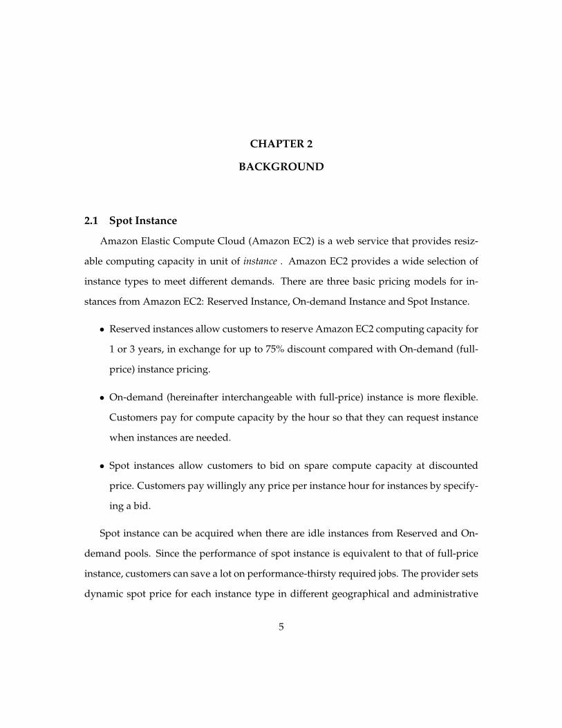
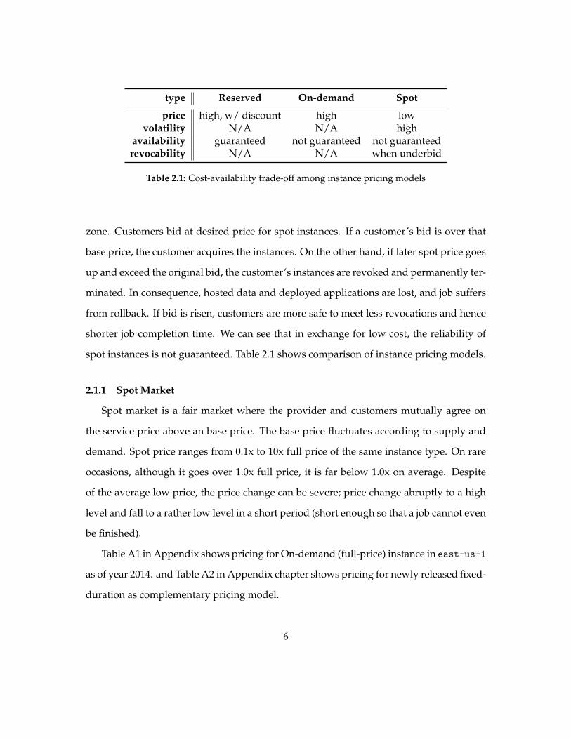
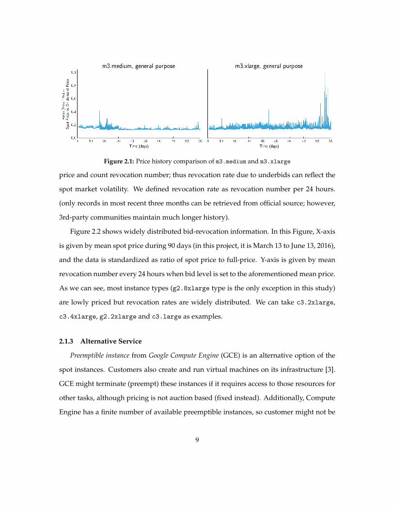
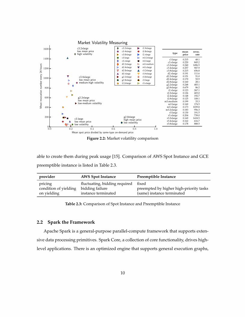
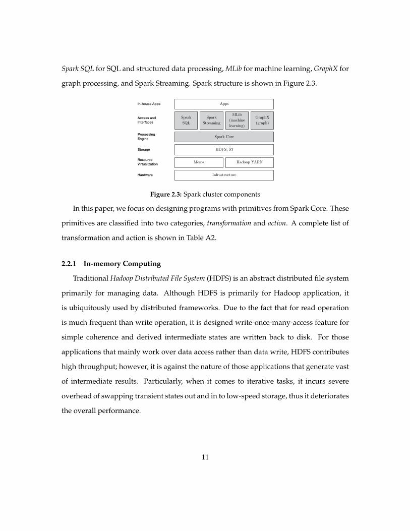
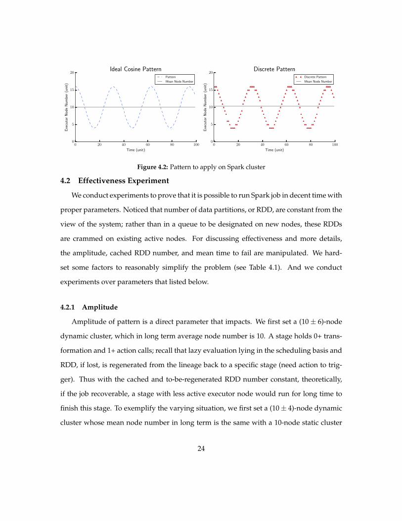
0 20 40 60 80 100
Time (unit)
0
5
10
15
20
Exe
cuto
rN
ode
Num
ber
(uni
t)Ideal Cosine Pattern
Pattern
Mean Node Number
0 20 40 60 80 100
Time (unit)
0
5
10
15
20
Exe
cuto
rN
ode
Num
ber
(uni
t)
Discrete PatternDiscrete Pattern
Mean Node Number
Figure 42 Pattern to apply on Spark cluster
42 Effectiveness Experiment
We conduct experiments to prove that it is possible to run Spark job in decent time with
proper parameters Noticed that number of data partitions or RDD are constant from the
view of the system rather than in a queue to be designated on new nodes these RDDs
are crammed on existing active nodes For discussing effectiveness and more details
the amplitude cached RDD number and mean time to fail are manipulated We hard-
set some factors to reasonably simplify the problem (see Table 41) And we conduct
experiments over parameters that listed below
421 Amplitude
Amplitude of pattern is a direct parameter that impacts We first set a (10plusmn 6)-node
dynamic cluster which in long term average node number is 10 A stage holds 0+ trans-
formation and 1+ action calls recall that lazy evaluation lying in the scheduling basis and
RDD if lost is regenerated from the lineage back to a specific stage (need action to trig-
ger) Thus with the cached and to-be-regenerated RDD number constant theoretically
if the job recoverable a stage with less active executor node would run for long time to
finish this stage To exemplify the varying situation we first set a (10plusmn 4)-node dynamic
cluster whose mean node number in long term is the same with a 10-node static cluster
24
parameters how it affects
performance instatic cluster
Performance in the static cluster outlines the best performancethat can be possibly achieved in the dynamic cluster In the dy-namic cluster if there is no node failure and thus rollback jobcompletion by stage whose time determined by the performancein the static cluster would not be repeated So avoiding revocationas much as possible lead to optimal results
timeout Timeout is criterion for the system to terminate the job and timelimit within which node connectivity issues must be resolved Bydefault after three attempts on reconnection with the failed nodethe current job will be killed by driver program
CPU core More available CPU cores are almost positive for everythingIn our experiment we restricted CPU core per node (usingm3medium instances)
checkpointwrite
Checkpointed job does not need to start over However if there isno failure checkpoint write time is wasteful In the effectivenessexperiment to test if Spark without high-latency checkpointingcan complete jobs
Table 41 Factors that potentially affect resilience
without node loss and addition Later a change in amplitude are discussed Results of
these sub-experiments are stated in Chapter 6
422 Parallelism Degree
Cached RDD number (or parallelism degree) in total is set to 20 making maximum of
hosted RDD number on each executor node less than 20 By default an equivalent CPU
core can process 2 RDDs at the same time thus as active node decreases average number
of RDD hosted on executor node exceeds 20 and simply lengthen job completion time
for this stage by at least 100 There is also an auxiliary experiment to see how RDD per
node impacts performance
25
423 Mean Time to Failrevoke
The interval or mean time to failrevoke is the key impact from the exterior envi-
ronments and whether the Spark cluster could recover from the turbulent technically
depends on whether the capacity to recover meet the deadline (there is a timeout in the
system)
424 Mean Time to Write Checkpoint
Later when we combined usage of both lineage and traditional checkpoint mecha-
nisms how often we conduct checkpoint write also affect Spark cluster performance
From [13] we know that for a single-node batch-job the job completion time is given
by
Tw(τ) = Ts︸︷︷︸solve time
+
(Ts
τminus 1)
δ︸ ︷︷ ︸checkpointing
dump time
+ [τ + δ] φ(τ + δ) n(τ)︸ ︷︷ ︸recovery time
+ Rn(τ)︸ ︷︷ ︸restart time
(41)
where Ts denotes job completion time without failure (solve time) n(τ) interruption time
δ time to write a checkpoint file φ(τ + δ) fraction of interruption averagely and R time
to restart And the optimum of mean time to write checkpoint is given by τopt =radic
2δM
where M denotes mean time to interrupt Not only can it be used for verification that
the simulator reflects real-world cases we expect to extend its scope to distributed cases
On the other hand when real history price is used to simulate the cluster Equation 41
does not quite apply any more and hidden mathematically representation is still to be
discovered
43 Simulator
For real-world tasks it takes at least 10 minutes to finish a task and even longer time
to repeatedly get reasonable result with less deviations To speed up development we
26
Partition life cycle
commit changes
try launching new nodes
process partitions
latest checkpoint
finished
exception caught
sync-eddesignate partitionsstart
checkpoint disabled
checkpoint enabled
(stage+1)
exitlaunched
interruption
Simplified cluster life cycle
Presumedly during one job there is no repartitioning and a partition is not annihilated when its hosted node is revoked
designated sync-edbeing processed
latest checkpoint
finishedstart
exception caught
checkpoint
disabled
checkpoint enabled
(stage+1)
exitlaunched
Figure 43 Simpler cluster life cycle description
designed a simulator An intuitive idea to simulate the cluster is to multithread the sim-
ulator program In details we can deploy one thread for driver node and multiple for
executor nodes However to stick with the goal rather than simply emphasize on the
mechanism or implementation as well as ability to extend the program in the future we
prioritize the observation of partition progress in comparison node is container where
partitions of workload is hosted and node life cycle that later as we can see could be
logically integrated as a whole cluster
In Figure 41 we can see that life cycle mostly coincides with executor node in the
cluster except for the partition is designed to live until the job is finished After tentatively
implementing a multi-threading prototype we found it was neither easy to extend nor
necessary 1) stage completion time for an iteration is determined by the longest partition
processing time from a specific node in the cluster thus the competing process is trivial
to record in the simulator and 2) cost exists as long as instances are on Thus in sense
of optimization we can simply calculate the longest processing time for that stage And
27
checkpoint mechanism would pause the processing thus processing and checkpoint if
any are executed in serial under the scheduling from driver node Thus a much simpler
as well as much faster single-threaded simulator is implemented from the angle of the
while cluster In the description of the cluster we focus on how partition state is transited
See details in Figure 43
28
CHAPTER 5
IMPLEMENTATION
Most parts for this project is implemented in Python Shell Script and illustrative ap-
plications are in Scala Also project platform is available and open-sourced at https
githubcomJonnyCEproject-platform And this chapter is organized in three parts
1) Cluster setting 2) platform and 3) pattern-based controller implementation
51 Cluster Setup
Components listed in Table 51 are necessary to set up a cluster Unfortunately there
is no handy deploy tool from Amazon official in fact Amazonrsquos command line tools
are quite fault-prone when deploying manually At this stage we use both Spark EC2
(released by Spark group) and implemented console tools based on Python Boto 238
and this will be the part comprising our abstraction interface
component version usage
Spark 12x or 13x Framework where applications submittedHDFS Hadoop 24+ Delivering distributed file systemMesos 0180 or 0210 Working as resource allocatorYARN Hadoop 24+ Mesos alternative negotiator
Scala 210 Front end for Java runtimePython 26+ Boto 2 package is employed for customization
Java 6+ Backend for Hadoop Scala and SparkBash built-in Built-in script interpreter
Table 51 Components and compatibility
29
bull EC2 Spot Instances With a pool of spot instances [1] we can request flexible number
of node to use At this stage we use Spark official EC2 deployment tool to automate
authorization between driver and executor nodes To manipulate the execute node
an ancillary control panel is also implemented based on AWS Boto API and Secure
Shell (SSH) pipe as supplement And to deliver better performance in the effective-
ness experiment we employ a m3large instance as driver node and m3medium as
executor instances
bull Storage Master-slave modeled HDFS cluster consists of a single namenode that man-
ages the file system namespace and regulates access to file by clients and a number
of datanode HDFS exposes a file system namespace and allows user data to be
stored in files [7] The existence of a single HDFS namenode in a cluster simplifies
the architecture of the system the namenode is designed to be the arbitrator and
repository for all HDFS meta-data and user data never flows through the namenode
In this paper We presume that the HDFS cluster (storage) the Spark cluster do not
overlap At this stage we also can use AWS S3 Bucket for easier deployment
Now we host Spark application (jar) with experiment dataset and tarball of Spark
framework in the bucket
bull Resource Allocator Mesos or YARN could be used to multiplex resource usage due to
the essence that there are multiple frameworks running on each single node Mesos
is designed to offer resources and collect feedback (accepted or refused) from multi-
tenant frameworks which do nothing against the nature of frameworks [17] Yet
YARN is an alternative choice that we did not take a close look at To port Mesos on
our target operating system we compiled Mesos of both 0180 and 0210 and one
of them is chosen to be installed as default one
30
Spark the Framework This experiment is to focus on fault tolerance and resilience fea-
tures of Spark Among different distributions of Spark we choose binary package
that is pre-built for Hadoop 24+ And two most recent versions 122 and 131 in
regard to compatibility
bull Control panel We have implemented different components for this project platform
shown in Table 52
component description
console based on AWS Boto 238 to request lookups and make snap-shotuser image on current cluster
experiment a spot market request simulator generating and propagating avail-ability pattern to the Spark framework
logger recording and analyzing availability pattern impactgraphic library supporting data visualizationmath library containing price analysis tools
Table 52 Control panel
bull PageRank demo application The lineage of example PageRank consists 13 stages 2
distinct actions 10 flatmap transformations for there are 10 iterations and 1 collect
action
bull Cluster setting The cluster is set as shown in Table 53 Noticed that time factor setting
is based on such a cluster In the experiments based on simulation in Section 63 a
time unit (40 seconds) is based on stage completion time
52 Simulator Implementation
The behavioral pseudo-code for the simulator essence is list below
The simulator as core part of the experiment is implemented in C++ for better perfor-
mance while analytical jobs are done in Python and shell scripts
31
overview driver m3large
executor m3medium with 24 GiB memory per node for Sparkworker
usage cores unlimited 10 for most of timememory 300 to 500 MiB128 GB in totaldisk 0 B for we did not set up checkpoint write
application description PageRank with 10 iterationsvariable iteration count in this case we set it constant 10 partition
number as known as RDD caching degree or degree of par-allelism
language Scala 210 with Java 17 as backendpackage jar package to submit
dataset source httpssnapstanfordedudataweb-Googlehtml
filesystem hosted on S3 bucket s3nspark-data-sampleweb-
Googletxt
description containing 875713 nodes 5105039 edges
Table 53 Cluster setting
1 initialization
2
3 while not all partitions finished processing
4 if time to interrupt
5 chosen victim nodes are down
6 hosted partitions roll back to checkpoint
7
8 if iteration -based
9 select only lagging partitions to resume
10 else
11 select all partitions to resume
12 designate corresponding partitions to active nodes
13
14 overhead of resume applied if any
15 bring back nodes if appropriate
16 process partitions
17
18 if checkpoint enabled and time to write
19 checkpoint write
20
21 done
32
CHAPTER 6
EVALUATION
61 Evaluation of Effectiveness Experiment
Job completion time is lengthened when there is loss and fallback and varies according
to specific parameters Presumably there is no re-partitioning that changes parallelism
degree ie partition number of a task In a dynamic cluster with constant compute
capacity of a single node (we only focus on CPU related capacity) stage completion time
always varies due to fluctuating node number of the cluster
Quantitatively we set a cluster of constant 10 nodes or a 10-node static cluster as
pivot In the effectiveness experiment we set a node number fluctuating according to
a periodic pattern with average value 10 ie a cluster of (10 plusmn m) nodes With such
technique in sense of node availability (the number of available node for computing)
these two clusters are at the same cost in average Nevertheless a (10plusmnm)-node cluster
should not be the equivalence of a 10-node static cluster a (10+ m)-node cluster loses 2m
nodes due to revocations on purpose
We would show the impacts from multiple aspects
bull Amplitude of the node availability varies in different scenarios a 10 plusmn m1- and a
10plusmn m2-node cluster (m1 6= m2) share the same cost on average if running for the
same time in the long term However to finish a exactly same jobs the completion
time may varies
33
bull An implication of node availability decrement undermines performance such a
decrement happens in the descending phase of the pattern If there is no change
in node availability and the node number remains at a certain level the completion
time is only determined by the workload and compute capacity And if the dynamic
cluster within a short duration the average compute capacity is the same with one
in the static cluster but job completion time increases we assume there is extra over-
head for node availability fluctuation
bull Reservation of always on node (unfinished) There has been discussion on whether
to employ always-on node to guarantee the performance or not For the sake of
simplicity only an illustration is shown in Figure 62 and we choose not to utilize
such alway-on instances for simplicity
611 Base Completion Time
To settle the question of existence of overhead from node availability change we first
measured job completion time in a static cluster as pivot Job completion time comprises
each stage completion time To standardize we measured stage completion time where
constant partitions are mapped onto various number of executor nodes And such mea-
surement guided the development of the simulator for parameter configuration The
static cluster for measuring base completion time is configured as 1) 10 m3medium ex-
ecutor nodes or 10 active CPU cores 2) each instance has 1 CPU core able to process 2
partitions in the same time and 3) demo MapReduce application contains 10 iterations
Job completion time is shown in Table A5 and Figure 61
In this experiment we designated 20 partitions onto 10 nodes As partition number
is increased from 2 to 20 job completion time drops hosted partition number decreased
from 100 to 10 Noticed that stage completion time slightly increases when less than 20
34
partitions are hosted on a CPU core on average In addition job completion time sum
total is approximately the same as what is given in the Spark WebUI (a built-in graphical
control panel) Result is shown in Table A5 and Figure 61
2 3 4 5 6 7 8 9 10 11 12 13 14 15 16 17 18 19 20
Partitioncached RDD number (unit)
0
75
150
225
300
375
450
Tim
e(s
econ
d)
40361
23009
12154
10873
10049
9259
8592
7829
6801 89168576
81837967
78657595
73157262
71257403
Mean time of PageRank application against parallelism degreemaster m3large slave m3medium
Figure 61 Figure for Table A5
612 Job Completion in Dynamic Cluster
In the effectiveness experiment we applied a pattern to node availability to a cluster
with at most 10 + m executor nodes making it a dynamic cluster And there is no extra
fault tolerance mechanisms applied except the internal one We set the amplitude of pat-
tern from 4 6 8 making the (maximum minimum) of a cluster node number (14 6)
(16 4) and (18 2) respectively For each case we also set comparison of cases with and
without reserved always-on nodes in the cluster The discrete pattern is in unit of 30
seconds node number is changed compulsorily every 30 seconds Below 30 seconds re-
vocation is intensified and the cluster can hardly recover and exceed the timeout caused
by cascading fallback Timeline of each case is shown in Figure 62 and it shows the feasi-
bility of completing job with appropriate parameters
We ran the same application (10 iterations) in the dynamic cluster for four times Trend
shows that small drop from maximum of the pattern lead to shorter completion time
Comparing a (10plusmn 4)- and a (10plusmn 6)-node cluster we noticed that gap in performance
35
is small and even negligible with these case study however a (10plusmn 8)-node alteration
shows obvious violation on the executing and the completion time is lengthened much
more in contrast to (10 plusmn 4) case Trend also shows that running job in the ascending
phase of the pattern is much shorter than in the descending phase which is intuitive and
expected Nevertheless in this illustrative evaluation we accessed to full control over
the node availability otherwise in the real-world we cannot predict on the phase change
of the market and the alteration of price is not gradually but abruptly Moreover the
absolute overhead is dense even the (10plusmn 4) cluster ran the task for much longer time
than the bad cases shown in Figure 61 Such a result can be attributed to the lack of proper
fault-tolerant mechanisms
In addition reserved always-on (on-demand) instances boost the performance And
on rare occasions if node availability is extremely low and memory capacity is far more
below abundant even loading dataset on need basis cannot be smooth rather virtual
memory swapping between memory and disk is automatically invoked and the latency
is magnified In sense of guaranteeing enough memory capacity always-on instances can
be put into use However on balancing the complexity of design the cost and income
and such technique is not applicable to all types of jobs We proceed later experiments
without such technique
62 Impacts of Parameters
In each experiment we have 3 dynamic cluster with different pattern amplitude a
single parameter is varying while others are unaltered Also in each experiment consists
of at least 20 submissions of the example PageRank application To simulate the real-word
cases we submit application to the cluster at arbitrary phase of periodical availability
pattern
36
0 20 40 60 80 100 120 140
Compulsory alterations (unit time = 30 seconds)
0
5
10
15
20
No
denu
mb
erImpact on Run Time from Pattern Amplitude
14 RDDs 10plusmn4 nodes
14 RDDs 10plusmn6 nodes
14 RDDs 10plusmn8 nodes
00 mins 140 mins 56 mins 130 mins 62 mins
00 mins 140 mins 51 mins 150 mins 52 mins
00 mins 200 mins 200 mins 200 mins
00 mins 120 mins 51 mins 140 mins 64 mins
00 mins 130 mins 51 mins 140 mins 51 mins
00 mins 180 mins 200 mins 200 mins
timeline 14 RDDs 10plusmn4 nodes
timeline 16 RDDs 10plusmn6 nodes
timeline 18 RDDs 10plusmn8 nodes
timeline w On-demand nodes 14 RDDs 10plusmn4 nodes
timeline w On-demand nodes 16 RDDs 10plusmn6 nodes
timeline w On-demand nodes 18 RDDs 10plusmn8 nodes
Figure 62 Running time in dynamic cluster
So far we gain some illustrative results as shown in Figure 63 The first figure shows
the impact on job completion time by changing MTBA Trending is that longer MTBA
interval leads to smaller variance of job completion time although sometimes some scat-
tered cases have much longer job completion time The second figure shows the impact
on job completion time by changing lineage length in this case the iteration number The
trending reflects the correctness of intuition that either larger amplitude (corresponding
to less availability) or longer iteration makes cluster even harder to recover If we compare
amplitude varying and iteration varying separately we find that variance beyond 25 to 75
percentile increasing holds although as iteration number increases monotonicity of job
completion time within 15 IQRs no longer valid The third figure shows the impact on
job completion time by changing partition number It is straight forward that increasing
parallelism degree from 10 to 20 leads to lower overhead and faster time finishing job Yet
it is not always valid that amplitude increasing surely deteriorate recovery More scrutiny
is needed on this part
37
10plusmn 230s
10plusmn 260s
10plusmn 430s
10plusmn 460s
10plusmn 630s
10plusmn 660s
200
300
400
500
600
700
800
900
1000
1100
Run Time Comparison30- and 60-second-MTTR
10plusmn 210p
10plusmn 220p
10plusmn 410p
10plusmn 420p
10plusmn 610p
10plusmn 620p
200
400
600
800
1000
1200
Run Time Comparison10- and 20-partition
10plusmn 210i
10plusmn 220i
10plusmn 410i
10plusmn 420i
200
400
600
800
1000
1200
1400
Run Time of Comparison10- and 20-iteration
Figure 63 Parameter impacts on job completion time
63 Results from Simulation
Verification With inspiration of optimization in single-node batch-job case we were to
apply optimum for distributed jobs Before that we first verified the simulator by running
a single-node batch job After the correctness is proven we extended the experience to
distributed cases and conducted a simple MapReduce to gain result and it turned out to
be applicable Both cases are under such restrictions 1) revocation occurrence satisfies the
approximation of Poisson distribution 2) a state of the job at one moment is dependent
on previous states and 3) revocation failure rate is proper such that with checkpoint write
a job could be finished Both cases are shown in Figure 64
Figure 64 Verification and extension
38
Experiments based on simulation From the actual execution on real Spark Instances
we gathered some data 1) in a static cluster stage completion time is around 40 seconds
when average RDD number on an executor node is less than 20 and 2) Spark cluster can
recover from a revocation every 30 seconds averagely (based on both pre-selected pattern
and Poisson Distribution) With these a posteriori experience we did some case studies
with simulations of m3large instance and we get some sample results listed below And
these results are main patterns selected various experiments
In Figure 65 we can see that overall trend shows that overhead from checkpoint write
impact on performance when checkpoint writing too frequently but alleviated when the
write interval set to appropriate value however when there are inadequate checkpoints
severe performance deterioration takes place and becomes even worse when checkpoint
write is towards absolutely absent Thus we see a small drop to local minimum in both
job completion time and total cost and it becomes global minimum
Figure 66 shows a pattern that resembles one in Figure 65 As we can see the pattern
goes flat because there is the short duration of price alteration where limited revocations
impact on job completion time thus total cost
In Figure 67 we see that at bid of 016x like patterns shown in Figure 65 and Fig-
ure 66 a small drop occurs leading to local minimum in both job completion time and
total cost after that both rises Another observation is that when we slightly rise the bid
we can see then the only overhead is from routine checkpoint write
Figure 66 shows drop and steady trending toward situation in which there is no
checkpoint write This is attributed to constant number of revocations exist during the
job processing Recall that if there are cascading revocations Spark may hit timeout and
failed the job (see Section 212) So we use this to determine to what degree shorter com-
pletion time and cost saving can be achieved In this case with mixed fault tolerance
39
scheme ˜20 shorter completion time and ˜25 lower cost are achieved than the situation
of no checkpoint write and compared with cases of running jobs on full-price instance
the absolute saving in costs can be ˜75
0 50 100 150 200
Checkpoint Write Interval (40 secondsunit)
250
300
350
400
450
500
Run
Tim
e
m3large l50 m09 b019 rarr 017
run time w bid019x
run time w bid018x
run time w bid017x
0 50 100 150 200
Checkpoint Write Interval (40 secondsunit)
450
500
550
600
650
700
750
800
Tot
alC
ost
run time w bid019x
run time w bid018x
run time w bid017x
Figure 65 Pattern of small drop 1
0 50 100 150 200
Checkpoint Write Interval (40 secondsunit)
260
280
300
320
340
360
380
400
420
440
Run
Tim
e
m3large l50 m26 b016 rarr 014
run time w bid016x
run time w bid015x
run time w bid014x
0 50 100 150 200
Checkpoint Write Interval (40 secondsunit)
360
380
400
420
440
460
480
500
520
Tot
alC
ost
run time w bid016x
run time w bid015x
run time w bid014x
completion time cost
bid minoverhead maxoverhead trending mindiscounted maxdiscounted trending
016 260 215 342 598 342 598 375 175 508 237 500 234015 304 421 370 729 370 729 392 183 500 234 500 234017 337 575 425 986 425 986 400 187 517 242 571 267
Figure 66 Pattern of small drop and constant
Noticed that result can be changed a lot when parameters are slightly tweaked For
example starting timeframe can lead to good or bad timing when encountering price
change and d grace period also contributes to the timing
Presumably all clusters go through revocations We conclude that
40
0 50 100 150 200
Checkpoint Write Interval (40 secondsunit)
150
200
250
300
350
400
450
500
550
600
Run
Tim
em3large l50 m01 b020 rarr 016
run time w bid020x
run time w bid019x
run time w bid018x
run time w bid017x
run time w bid016x
0 50 100 150 200
Checkpoint Write Interval (40 secondsunit)
300
400
500
600
700
800
900
Tot
alC
ost
run time w bid020x
run time w bid019x
run time w bid018x
run time w bid017x
run time w bid016x
completion time cost
bid minoverhead maxoverhead trending mindiscounted maxdiscounted trending
020 NA 250168 21505 NA 295138 400187019 NA 260215 23598 NA 485227 440206018 NA 275285 260215 NA 460215 440206017 NA 285332 280308 NA 440206 440206016 320495 6001804 NA 420196 850397 NA
Figure 67 Price-sensitive pattern
1 Optimum checkpoint write interval tends to be small ie overhead from checkpoint
write is much smaller than that from rolling back with RDD recovery
2 The robust of checkpointing in sense of interval could help lower the price of using
spot instances and work according to market information
3 Sometimes a small rise in bid can lead to qualitative change and lower bid does not
always mean lower cost
41
APPENDIX A
SPOT INSTANCE PRICE RECORDS
purpose type vCPU ECU RAM (Gib) disk (GB)price according to usage (USD per hour)
LinuxUNIX Windows w SQL
general RHEL SUSE general std web
general t2micro 1 var 1 EBS Only 001 007 002 002 007t2small 1 var 2 EBS Only 003 009 006 004 014t2medium 2 var 4 EBS Only 005 011 015 007 027t2large 2 var 8 EBS Only 010 016 020 013 043m3medium 1 3 375 1 x 4 SSD 007 013 017 013 035 018m3large 2 65 75 1 x 32 SSD 013 019 023 026 070 037m3xlarge 4 13 15 2 x 40 SSD 027 033 037 052 127 073m32xlarge 8 26 30 2 x 80 SSD 053 066 063 104 253 147m4large 2 65 8 EBS Only 013 019 023 025 093 026m4xlarge 4 13 16 EBS Only 025 031 035 050 112 044m42xlarge 8 26 32 EBS Only 050 063 060 101 235 090m44xlarge 16 535 64 EBS Only 101 114 111 202 464 184m410xlarge 40 1245 160 EBS Only 252 265 262 504 1181 458
compute c3large 2 7 375 2 x 16 SSD 011 017 021 019 056 027optmized c3xlarge 4 14 75 2 x 40 SSD 021 027 031 038 107 054
c32xlarge 8 28 15 2 x 80 SSD 042 055 052 075 213 108c34xlarge 16 55 30 2 x 160 SSD 084 097 094 150 426 217c38xlarge 32 108 60 2 x 320 SSD 168 181 178 301 852 433c4large 2 8 375 EBS Only 011 017 021 019 141 042c4xlarge 4 16 75 EBS Only 022 028 032 039 168 079c42xlarge 8 31 15 EBS Only 044 057 054 077 335 164c44xlarge 16 62 30 EBS Only 088 101 098 155 558 223c48xlarge 36 132 60 EBS Only 176 189 186 309 1257 427
GPU g22xlarge 8 26 15 60 SSD 065 078 075 077 382 096instance g28xlarge 32 104 60 2 x 120 SSD 260 273 270 288
memory r3large 2 65 15 1 x 32 SSD 018 024 028 030 096 040optmized r3xlarge 4 13 305 1 x 80 SSD 035 041 045 060 140 076
r32xlarge 8 26 61 1 x 160 SSD 070 083 080 108 278 156r34xlarge 16 52 122 1 x 320 SSD 140 153 150 194 466 237r38xlarge 32 104 244 2 x 320 SSD 280 293 290 350 876 400
storage i2xlarge 4 14 305 1 x 800 SSD 085 091 095 097 123 099optmized i22xlarge 8 27 61 2 x 800 SSD 171 184 181 195 246 199
i24xlarge 16 53 122 4 x 800 SSD 341 354 351 389 492 397i28xlarge 32 104 244 8 x 800 SSD 682 695 692 778 984 794d2xlarge 4 14 305 3 x 2000 HDD 069 075 079 082d22xlarge 8 28 61 6 x 2000 HDD 138 151 148 160d24xlarge 16 56 122 12 x 2000 HDD 276 289 286 306d28xlarge 36 116 244 24 x 2000 HDD 552 565 562 620
Table A1 east-us-1 On-demand instance pricing
42
data collected at 1116 PM on October 8 2015 us-east-1
type discounted price type discounted price
spot 1-hr fixed 6-hr fixed spot 1-hr fixed 6-hr fixed
m3medium 14 55 70 c4xlarge 15 55 70m3large 20 55 70 c42xlarge 17 55 70
m3xlarge 15 55 70 c44xlarge 16 55 70m32xlarge 14 55 70 c48xlarge 23 55 70
m4large 12 55 70 d2xlarge 10 55 70m4xlarge 11 55 70 d22xlarge 11 55 70
m42xlarge 11 55 70 d24xlarge 10 55 70m44xlarge 12 55 70 d28xlarge 11 55 70
m410xlarge 14 55 70 g22xlarge 11 55 70c3large 16 55 70 g28xlarge 18 55 70
c3xlarge 18 55 70 r3large 15 55 70c32xlarge 20 55 70 r3xlarge 14 55 70c34xlarge 19 55 70 r32xlarge 20 55 70c38xlarge 19 55 70 r34xlarge 3 55 70
c4large 16 55 70 r38xlarge 11 55 70
Table A2 east-us-1 Spot and Fixed-duration instance pricing
bid c32xl c34xl c38xl c3l c3xl d22xl d24xl d28xl d2xl g22xl g28xl
012 420830 394177 288994 83622 311636 29173 17089 11763 24548 295292 70653013 420830 394177 288994 83622 311636 16337 12582 8646 23132 281510 70486014 420830 394177 288994 83622 311636 9153 9993 5824 21829 251651 70134015 420830 394177 288994 83622 311636 5186 7076 3393 20358 218304 69192016 420830 393480 283578 79531 310872 4096 6023 2738 18141 190016 67666017 419854 384284 228962 41747 285920 3180 5252 1951 14942 162976 65506018 409547 359443 170328 19952 234102 2569 4423 1127 12790 139420 62241019 376373 318954 127056 10940 181431 2358 3907 1010 11163 115924 58904020 330816 271954 96624 7484 137286 1941 3363 747 9573 99044 54297021 276384 226020 73217 5479 105086 1678 2884 544 8003 84039 51172022 225029 184471 56076 4229 81573 1432 2657 437 7114 72126 48478023 182061 150837 43627 3168 64733 1227 2134 369 6141 61810 45791024 145820 123452 33792 2661 51717 1098 1908 336 5034 53199 43538025 117107 102290 26346 2272 42546 960 1840 311 4322 46284 41298026 93374 86198 19920 2003 35877 866 1662 308 3644 40056 39348027 73083 73129 14981 1757 30087 821 1589 304 3192 34127 36493028 57254 62368 12031 1618 25364 768 1536 303 2829 29603 35246029 44694 53890 9914 1464 21719 658 1313 247 2494 25620 32916030 34977 44766 8286 1376 18781 629 1272 237 2138 22619 31461031 26704 39998 7223 1274 16392 599 1117 233 1798 19120 29522032 21626 35872 6488 1214 14260 573 1093 229 1573 18084 28180033 17247 32646 5932 1169 12606 544 1066 229 1413 16557 27028034 13904 29604 5471 1132 10892 509 1050 227 1271 15662 25686035 11014 27064 4994 1104 9750 489 1027 226 1132 15016 24581036 8617 24652 4573 1068 8710 469 997 224 1047 14207 23374037 7061 22731 4270 1038 7850 437 961 224 994 13420 22081038 5817 20986 4002 1007 7060 429 936 224 902 13044 21307039 4767 19492 3772 972 6197 422 858 224 809 12157 17412040 4004 18093 3559 956 5589 416 843 224 739 11771 16946
Table A3 Market volatility 01 highlighted if 10 revocations per hour
43
bid i22xl i24xl i28xl i2xl m32xl m3l m3m m3xl r32xl r34xl r38xl r3l r3xl
012 50109 36649 11709 28246 325141 124554 49822 365960 384426 154518 262284 29483 244793013 32232 30662 8819 23222 324980 123191 48634 365548 341450 118836 227386 18021 206916014 19069 24062 6954 15923 313478 83416 34101 347844 284517 94461 192446 10787 173832015 9848 18238 4866 7539 268893 43116 24689 280906 228904 75998 158687 7454 146218016 5212 13567 2081 3129 208514 25697 18470 195868 180579 63766 129844 5427 124951017 2871 10433 1083 1422 148750 17009 12043 115116 138341 54606 105879 4277 109304018 1660 8787 973 294 102647 12363 7262 65877 106192 47558 84449 3479 95797019 1250 6929 902 293 71837 9168 4486 40611 83573 42097 63372 2881 85450020 1133 4820 833 223 50889 6963 2971 26124 65986 38120 52449 2503 76262021 1020 3411 759 211 37922 5464 2067 18114 53021 34424 43866 2172 68750022 964 2324 709 206 28466 4044 1588 12484 42658 31460 37076 1951 61924023 870 1930 638 130 21624 3151 1254 8901 34461 28427 31430 1729 56300024 760 1783 596 130 16346 2544 956 6478 28872 25880 26992 1566 51674025 701 1636 552 129 12339 2103 792 5066 24219 23783 23592 1451 47294026 599 1268 486 128 9477 1731 621 4231 20348 21854 20471 1328 43499027 572 1137 451 128 7192 1382 567 3740 17486 20168 18016 1186 40332028 549 1020 409 128 4936 1120 514 3518 15038 18651 15681 1104 37271029 538 914 373 101 4119 966 324 3237 13038 17411 13653 1054 34648030 517 777 352 101 3172 842 206 2966 11301 16209 11888 1009 32222031 452 706 292 098 2626 710 206 2558 9881 14893 10341 968 30122032 441 667 277 098 2160 610 206 2120 8582 13912 9268 853 27934033 423 633 266 098 1832 513 206 1684 7550 13038 8310 830 26126034 419 610 248 098 1467 423 206 1448 6661 12061 7447 800 24347035 401 580 242 098 1193 370 204 1314 5859 11262 6790 784 22826036 391 558 236 098 1009 320 204 1213 5062 10511 6223 763 21463037 388 542 229 098 872 283 204 1136 4292 9741 5748 741 20259038 371 507 222 098 754 251 204 1069 3600 8654 5203 721 19120039 277 431 206 096 611 237 204 1009 2953 8057 4829 706 18166040 274 413 197 096 579 233 204 960 2212 7446 4479 689 17071
Table A4 Market volatility 02 highlighted if 10 revocations per hour
RDD run timesecond statistics
caching 1st 2nd 3rd average upper error lower error
degree instance instance instance value percent value percent
2 399320 391292 420226 403613 16613 412 12321 3053 243068 219362 227840 230090 12978 564 10728 4664 122002 121276 121354 121544 0458 038 0268 0225 102479 117092 106608 108726 8366 769 6247 5756 97164 102284 102032 100493 1791 178 3329 3317 91984 90778 95010 92591 2419 261 1813 1968 87494 80876 89383 85918 3465 403 5042 5879 78674 77551 78640 78288 0386 049 0737 094
10 68813 68366 66861 68013 0800 118 1152 16911 88529 89188 89776 89164 0612 069 0635 07112 83776 88001 85499 85759 2242 261 1983 23113 81546 82397 81544 81829 0568 069 0285 03514 79858 78711 80425 79665 0760 095 0954 12015 77439 78753 79757 78650 1107 141 1211 15416 75719 75456 76676 75950 0726 096 0494 06517 73128 73595 72721 73148 0447 061 0427 05818 72592 72050 73233 72625 0608 084 0575 07919 71956 71341 70464 71254 0702 099 0790 11120 72473 74254 75373 74033 1340 181 1560 211
Table A5 Baseline job completion time
44
APPENDIX B
SPARK WORKING MODES
storage level description
MEMORY ONLY Store RDD as deserialized Java objects in the JVM If the RDD does not fit inmemory some partitions will not be cached and will be recomputed on the flyeach time theyrsquore needed This is the default level
MEMORY AND DISK Store RDD as deserialized Java objects in the JVM If the RDD does not fit inmemory store the partitions that donrsquot fit on disk and read them from therewhen theyrsquore needed
MEMORY ONLY SER Store RDD as serialized Java objects (one byte array per partition) This is gener-ally more space-efficient than deserialized objects especially when using a fastserializer but more CPU-intensive to read
MEMORY AND DISK SER Similar to MEMORY ONLY SER but spill partitions that donrsquot fit in memory to diskinstead of recomputing them on the fly each time theyrsquore needed
DISK ONLY Store the RDD partitions only on diskMEMORY ONLY 2
MEMORY AND DISK 2 Same as the levels above but replicate each partition on two cluster nodes
Table A1 Storage level of RDD
transformations
map( f Trarr U) RDD[T] rarr RDD[U]
filter( f Trarr Bool) RDD[T] rarr RDD[T]
flatMap( f Trarr Seq[U]) RDD[T] rarr RDD[U]
sample( f raction Float) RDD[T] rarr RDD[T] (Deterministic sampling)groupByKey() RDD[(K V)] rarr RDD[(K Seq[V])]
reduceByKey( f (V V)rarr V) RDD[(K V)] rarr RDD[(K V)]
union() (RDD[T] RDD[T]) rarr RDD[T]
join() (RDD[(K V)] RDD[(K W)]) rarr RDD[(K (V W))]
cogroup() (RDD[(K V)] RDD[(K W)]) rarr RDD[(K (Seq[V] Seq[W]))]
crossProduct() (RDD[T] RDD[U]) rarr RDD[(T U)]
mapValues( f VrarrW) RDD[(K V)] rarr RDD[(K W)] (Preserves partitioning)sort(c Comparator[K]) RDD[(K V)] rarr RDD[(K V)]
partitionBy(p Partitioner[K]) RDD[(K V)] rarr RDD[(K V)]
actions
count() RDD[T] rarr Long
collect() RDD[T] rarr Seq[T]
reduce( f (T T)rarr T) RDD[T] rarr T
lookup(k K) RDD[(K V)] rarr Seq[V] (On hashrange partitioned RDDs)save(path String) Outputs RDD to a storage system eg HDFS
Table A2 Transformations and actions
45
BIBLIOGRAPHY
[1] Amazon EC2 Instance Purchasing Options httpawsamazoncomec2
purchasing-options
[2] Amazon Elastic Compute Cloud httpawsamazoncomec2
[3] Google Compute Engine httpscloudgooglecomproductscompute-
engine
[4] Microsoft Azure httpsazuremicrosoftcom
[5] Sample Price History of Spot Instance httpsgithubcomJonnyCEproject-
platformtreemasterprice_history
[6] Spark Configuration httpsparkapacheorgdocslatestconfiguration
html
[7] Apache Hadoop HDFS Architecture httphadoopapacheorgdocscurrenthadoop-project-disthadoop-hdfsHdfsDesignhtml
[8] Apache Hadoop Project Hadoop mapreduce httphadoopapacheorgdocs
currenthadoop-project-disthadoop-hdfsHdfsUserGuidehtml
[9] Bu Yingyi Howe Bill Balazinska Magdalena and Ernst Michael D Haloop effi-cient iterative data processing on large clusters Proceedings of the VLDB Endowment3 1-2 (2010) 285ndash296
[10] Buyya Rajkumar Yeo Chee Shin and Venugopal Srikumar Market-Oriented CloudComputing Vision Hype and Reality for Delivering IT Services as Computing Util-ities arXivorg (Aug 2008)
[11] Chohan N Castillo C Spreitzer M and Steinder M See Spot Run Using SpotInstances for MapReduce Workflows HotCloud (2010)
[12] Daly John A model for predicting the optimum checkpoint interval for restartdumps In ICCSrsquo03 Proceedings of the 2003 international conference on Computationalscience (June 2003) Raytheon Springer-Verlag pp 3ndash12
46
[13] Daly John T A higher order estimate of the optimum checkpoint interval for restartdumps Future Generation Computer Systems 22 3 (2006) 303ndash312
[14] Ecole Polytechnique Federale de Lausanne (EPFL) Scala httpwwwscala-langorg
[15] Google Cloud Platform Preemptible Instancee httpscloudgooglecom
computedocsinstancespreemptible
[16] He Xin Shenoy Prashant Sitaraman Ramesh and Irwin David Cutting the costof hosting online services using cloud spot markets In Proceedings of the 24th Interna-tional Symposium on High-Performance Parallel and Distributed Computing (2015) ACMpp 207ndash218
[17] Hindman B Konwinski A Zaharia M and Ghodsi A Mesos A Platform for Fine-Grained Resource Sharing in the Data Center NSDI (2011)
[18] Institute for Telecommunication Sciences Federal Standard 1037C Glossary ofTelecommunications Terms - Avalibility httpwwwitsbldrdocgovfs-1037
fs-1037chtm
[19] Lagar-Cavilla Horacio Andres Whitney Joseph Andrew Scannell Adin MatthewPatchin Philip Rumble Stephen M de Lara Eyal Brudno Michael and Satya-narayanan Mahadev SnowFlock rapid virtual machine cloning for cloud computingACM Apr 2009
[20] Liu H Cutting MapReduce Cost with Spot Market HotCloud (2011)
[21] Malewicz Grzegorz Austern Matthew H Bik Aart JC Dehnert James C HornIlan Leiser Naty and Czajkowski Grzegorz Pregel a system for large-scale graphprocessing In Proceedings of the 2010 ACM SIGMOD International Conference on Man-agement of data (2010) ACM pp 135ndash146
[22] Mattess M Vecchiola C and Buyya R Managing peak loads by leasing cloud in-frastructure services from a spot market (HPCC) (2010) 180ndash188
[23] Salama Abdallah Binnig Carsten Kraska Tim and Zamanian Erfan Cost-basedFault-tolerance for Parallel Data Processing ACM New York New York USA May2015
[24] Sharma Prateek Irwin David and Shenoy Prashant How not to bid the cloudUniversity of Massachusetts Technical Report UMCS-2016-002 (2016)
47
[25] Subramanya Supreeth Guo Tian Sharma Prateek Irwin David and ShenoyPrashant SpotOn a batch computing service for the spot market In SoCC rsquo15Proceedings of the Sixth ACM Symposium on Cloud Computing (Aug 2015) Universityof Massachusetts Amherst ACM
[26] Yan Ying Gao Yanjie Chen Yang Guo Zhongxin Chen Bole and MoscibrodaThomas Tr-spark Transient computing for big data analytics accepted in 2016ACM Symposium on Cloud Computing 2016
[27] Yi S Kondo D and Andrzejak A Reducing costs of spot instances via checkpoint-ing in the amazon elastic compute cloud 2010 IEEE 3rd International (2010)
[28] Yi Sangho Kondo Derrick and Andrzejak Artur Reducing Costs of Spot Instancesvia Checkpointing in the Amazon Elastic Compute Cloud 2010 IEEE InternationalConference on Cloud Computing (CLOUD) (2010) 236ndash243
[29] Zaharia Matei Chowdhury Mosharaf Das Tathagata Dave Ankur Ma JustinMcCauley Murphy Franklin Michael J Shenker Scott and Stoica Ion Resilientdistributed datasets a fault-tolerant abstraction for in-memory cluster computingIn NSDIrsquo12 Proceedings of the 9th USENIX conference on Networked Systems Design andImplementation (Apr 2012) USENIX Association pp 2ndash2
[30] Zaharia Matei Chowdhury Mosharaf Franklin Michael J Shenker Scott and Sto-ica Ion Spark cluster computing with working sets In HotCloudrsquo10 Proceedingsof the 2nd USENIX conference on Hot topics in cloud computing (June 2010) USENIXAssociation
[31] Zhang Irene Garthwaite Alex Baskakov Yury Barr Kenneth C Zhang IreneGarthwaite Alex Baskakov Yury and Barr Kenneth C Fast restore of checkpointedmemory using working set estimation vol 46 ACM July 2011
[32] Zheng Liang Joe-Wong Carlee Tan Chee Wei Chiang Mung and Wang XinyuHow to Bid the Cloud In SIGCOMM rsquo15 Proceedings of the 2015 ACM Conference onSpecial Interest Group on Data Communication (New York New York USA Aug 2015)ACM Request Permissions pp 71ndash84
[33] Zhou Yanqi Wentzlaff David Zhou Yanqi Wentzlaff David Zhou Yanqi andWentzlaff David The sharing architecture sub-core configurability for IaaS cloudsACM SIGARCH Computer Architecture News 42 1 (Apr 2014) 559ndash574
48
- Analyzing Spark Performance on Spot Instances
-
- Recommended Citation
-
- Abstract
- List of Tables
- List of Figures
- Introduction
- Background
-
- Spot Instance
-
- Spot Market
- Market Volatility
- Alternative Service
-
- Spark the Framework
-
- In-memory Computing
- Resilient Distributed Datasets
-
- Fault Tolerance
-
- Recomputing from Lineage
- Node Failure Difference
- Naiumlve Fault Tolerance Scheme
- Checkpoint
- Mixed Fault Tolerance Scheme
-
- Related Works
-
- Cloud Computing
- Bidding the Cloud
- Fault Tolerance
-
- Design
-
- Cluster
-
- Driver Node Life Cycle
- Executor Node Life Cycle
- Job Classification
- Cluster Prototype
-
- Effectiveness Experiment
-
- Amplitude
- Parallelism Degree
- Mean Time to Failrevoke
- Mean Time to Write Checkpoint
-
- Simulator
-
- Implementation
-
- Cluster Setup
- Simulator Implementation
-
- Evaluation
-
- Evaluation of Effectiveness Experiment
-
- Base Completion Time
- Job Completion in Dynamic Cluster
-
- Impacts of Parameters
- Results from Simulation
-
- Spot Instance Price Records
- Spark Working Modes
- Bibliography
-
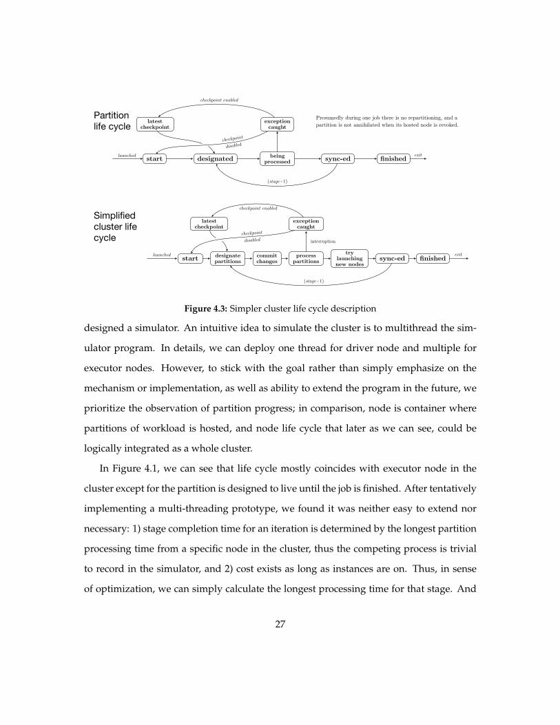
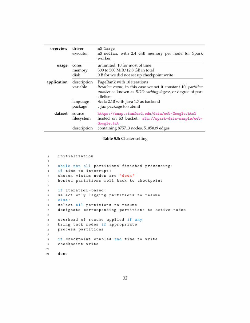
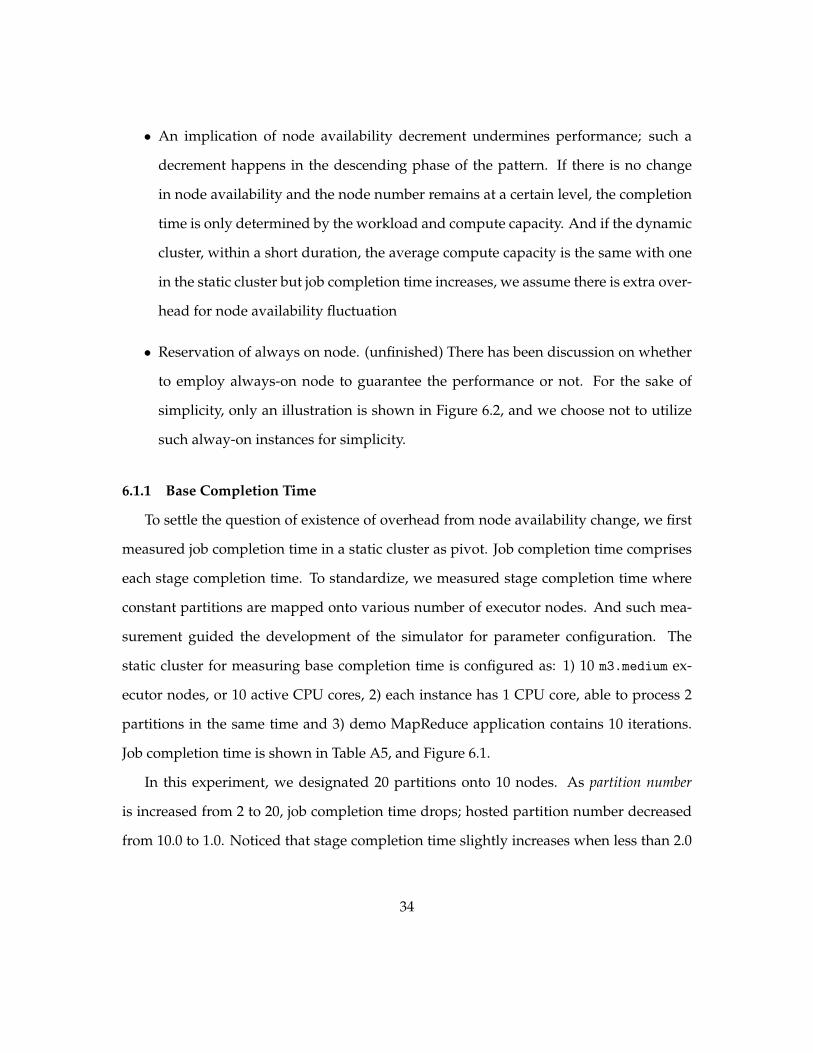
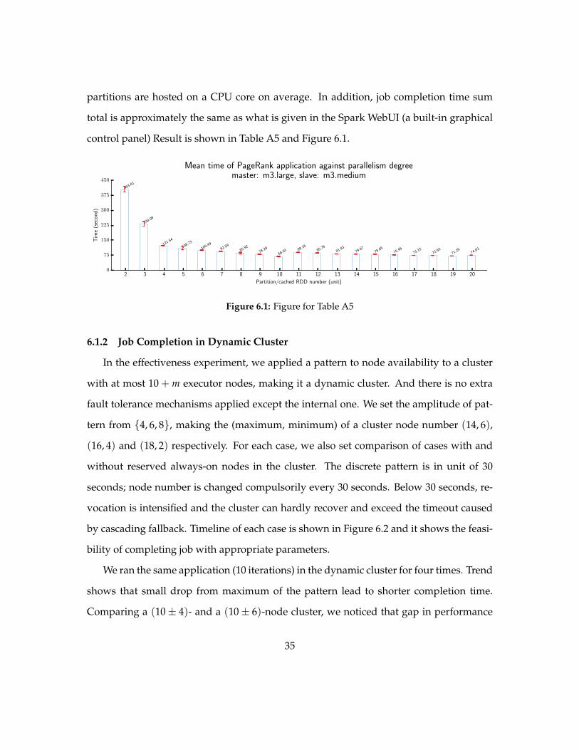
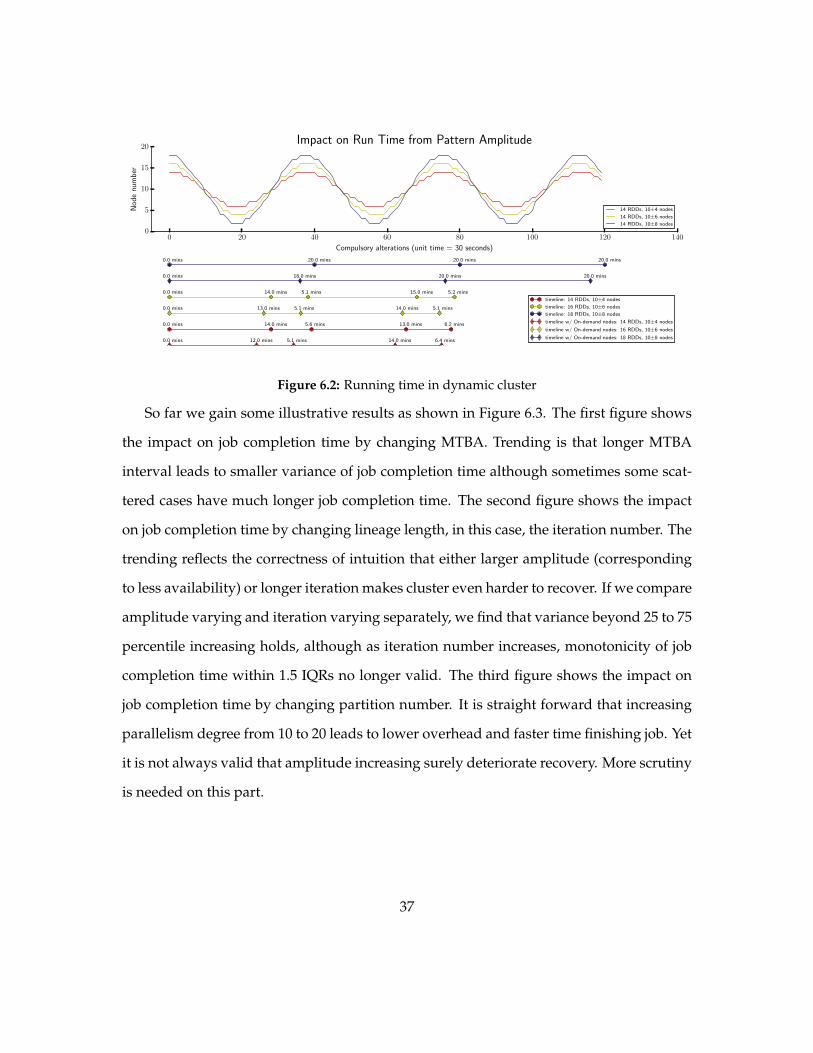
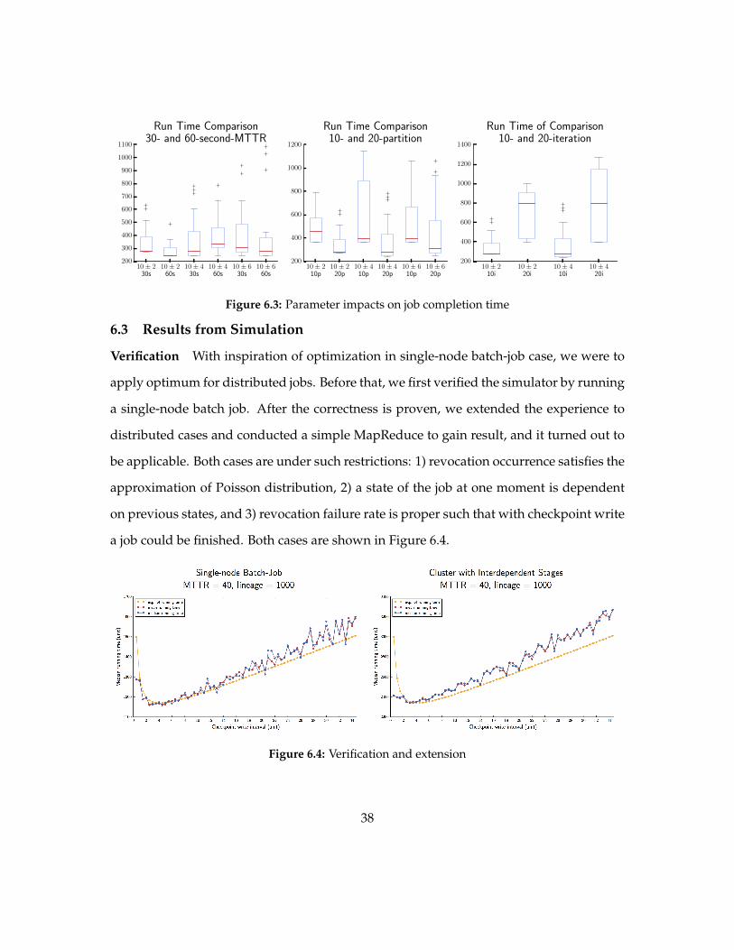
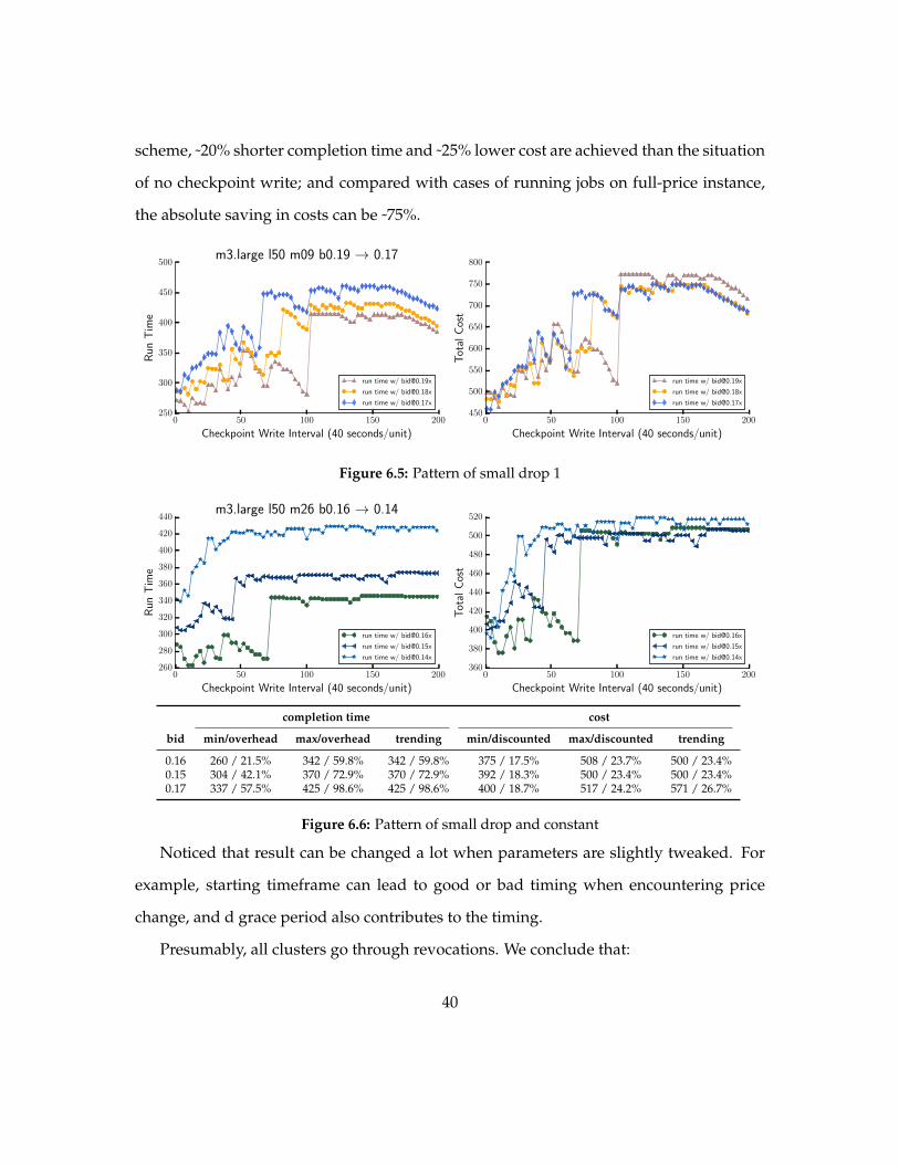
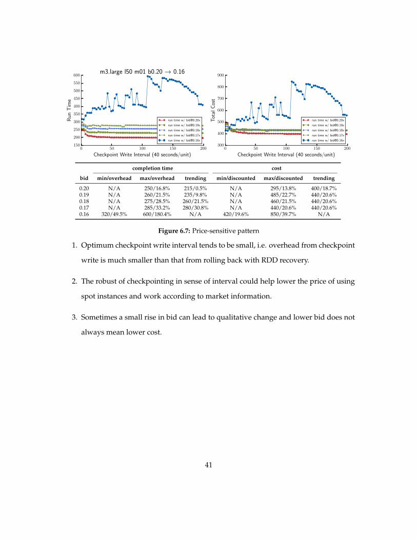
0 50 100 150 200
Checkpoint Write Interval (40 secondsunit)
150
200
250
300
350
400
450
500
550
600
Run
Tim
em3large l50 m01 b020 rarr 016
run time w bid020x
run time w bid019x
run time w bid018x
run time w bid017x
run time w bid016x
0 50 100 150 200
Checkpoint Write Interval (40 secondsunit)
300
400
500
600
700
800
900
Tot
alC
ost
run time w bid020x
run time w bid019x
run time w bid018x
run time w bid017x
run time w bid016x
completion time cost
bid minoverhead maxoverhead trending mindiscounted maxdiscounted trending
020 NA 250168 21505 NA 295138 400187019 NA 260215 23598 NA 485227 440206018 NA 275285 260215 NA 460215 440206017 NA 285332 280308 NA 440206 440206016 320495 6001804 NA 420196 850397 NA
Figure 67 Price-sensitive pattern
1 Optimum checkpoint write interval tends to be small ie overhead from checkpoint
write is much smaller than that from rolling back with RDD recovery
2 The robust of checkpointing in sense of interval could help lower the price of using
spot instances and work according to market information
3 Sometimes a small rise in bid can lead to qualitative change and lower bid does not
always mean lower cost
41
APPENDIX A
SPOT INSTANCE PRICE RECORDS
purpose type vCPU ECU RAM (Gib) disk (GB)price according to usage (USD per hour)
LinuxUNIX Windows w SQL
general RHEL SUSE general std web
general t2micro 1 var 1 EBS Only 001 007 002 002 007t2small 1 var 2 EBS Only 003 009 006 004 014t2medium 2 var 4 EBS Only 005 011 015 007 027t2large 2 var 8 EBS Only 010 016 020 013 043m3medium 1 3 375 1 x 4 SSD 007 013 017 013 035 018m3large 2 65 75 1 x 32 SSD 013 019 023 026 070 037m3xlarge 4 13 15 2 x 40 SSD 027 033 037 052 127 073m32xlarge 8 26 30 2 x 80 SSD 053 066 063 104 253 147m4large 2 65 8 EBS Only 013 019 023 025 093 026m4xlarge 4 13 16 EBS Only 025 031 035 050 112 044m42xlarge 8 26 32 EBS Only 050 063 060 101 235 090m44xlarge 16 535 64 EBS Only 101 114 111 202 464 184m410xlarge 40 1245 160 EBS Only 252 265 262 504 1181 458
compute c3large 2 7 375 2 x 16 SSD 011 017 021 019 056 027optmized c3xlarge 4 14 75 2 x 40 SSD 021 027 031 038 107 054
c32xlarge 8 28 15 2 x 80 SSD 042 055 052 075 213 108c34xlarge 16 55 30 2 x 160 SSD 084 097 094 150 426 217c38xlarge 32 108 60 2 x 320 SSD 168 181 178 301 852 433c4large 2 8 375 EBS Only 011 017 021 019 141 042c4xlarge 4 16 75 EBS Only 022 028 032 039 168 079c42xlarge 8 31 15 EBS Only 044 057 054 077 335 164c44xlarge 16 62 30 EBS Only 088 101 098 155 558 223c48xlarge 36 132 60 EBS Only 176 189 186 309 1257 427
GPU g22xlarge 8 26 15 60 SSD 065 078 075 077 382 096instance g28xlarge 32 104 60 2 x 120 SSD 260 273 270 288
memory r3large 2 65 15 1 x 32 SSD 018 024 028 030 096 040optmized r3xlarge 4 13 305 1 x 80 SSD 035 041 045 060 140 076
r32xlarge 8 26 61 1 x 160 SSD 070 083 080 108 278 156r34xlarge 16 52 122 1 x 320 SSD 140 153 150 194 466 237r38xlarge 32 104 244 2 x 320 SSD 280 293 290 350 876 400
storage i2xlarge 4 14 305 1 x 800 SSD 085 091 095 097 123 099optmized i22xlarge 8 27 61 2 x 800 SSD 171 184 181 195 246 199
i24xlarge 16 53 122 4 x 800 SSD 341 354 351 389 492 397i28xlarge 32 104 244 8 x 800 SSD 682 695 692 778 984 794d2xlarge 4 14 305 3 x 2000 HDD 069 075 079 082d22xlarge 8 28 61 6 x 2000 HDD 138 151 148 160d24xlarge 16 56 122 12 x 2000 HDD 276 289 286 306d28xlarge 36 116 244 24 x 2000 HDD 552 565 562 620
Table A1 east-us-1 On-demand instance pricing
42
data collected at 1116 PM on October 8 2015 us-east-1
type discounted price type discounted price
spot 1-hr fixed 6-hr fixed spot 1-hr fixed 6-hr fixed
m3medium 14 55 70 c4xlarge 15 55 70m3large 20 55 70 c42xlarge 17 55 70
m3xlarge 15 55 70 c44xlarge 16 55 70m32xlarge 14 55 70 c48xlarge 23 55 70
m4large 12 55 70 d2xlarge 10 55 70m4xlarge 11 55 70 d22xlarge 11 55 70
m42xlarge 11 55 70 d24xlarge 10 55 70m44xlarge 12 55 70 d28xlarge 11 55 70
m410xlarge 14 55 70 g22xlarge 11 55 70c3large 16 55 70 g28xlarge 18 55 70
c3xlarge 18 55 70 r3large 15 55 70c32xlarge 20 55 70 r3xlarge 14 55 70c34xlarge 19 55 70 r32xlarge 20 55 70c38xlarge 19 55 70 r34xlarge 3 55 70
c4large 16 55 70 r38xlarge 11 55 70
Table A2 east-us-1 Spot and Fixed-duration instance pricing
bid c32xl c34xl c38xl c3l c3xl d22xl d24xl d28xl d2xl g22xl g28xl
012 420830 394177 288994 83622 311636 29173 17089 11763 24548 295292 70653013 420830 394177 288994 83622 311636 16337 12582 8646 23132 281510 70486014 420830 394177 288994 83622 311636 9153 9993 5824 21829 251651 70134015 420830 394177 288994 83622 311636 5186 7076 3393 20358 218304 69192016 420830 393480 283578 79531 310872 4096 6023 2738 18141 190016 67666017 419854 384284 228962 41747 285920 3180 5252 1951 14942 162976 65506018 409547 359443 170328 19952 234102 2569 4423 1127 12790 139420 62241019 376373 318954 127056 10940 181431 2358 3907 1010 11163 115924 58904020 330816 271954 96624 7484 137286 1941 3363 747 9573 99044 54297021 276384 226020 73217 5479 105086 1678 2884 544 8003 84039 51172022 225029 184471 56076 4229 81573 1432 2657 437 7114 72126 48478023 182061 150837 43627 3168 64733 1227 2134 369 6141 61810 45791024 145820 123452 33792 2661 51717 1098 1908 336 5034 53199 43538025 117107 102290 26346 2272 42546 960 1840 311 4322 46284 41298026 93374 86198 19920 2003 35877 866 1662 308 3644 40056 39348027 73083 73129 14981 1757 30087 821 1589 304 3192 34127 36493028 57254 62368 12031 1618 25364 768 1536 303 2829 29603 35246029 44694 53890 9914 1464 21719 658 1313 247 2494 25620 32916030 34977 44766 8286 1376 18781 629 1272 237 2138 22619 31461031 26704 39998 7223 1274 16392 599 1117 233 1798 19120 29522032 21626 35872 6488 1214 14260 573 1093 229 1573 18084 28180033 17247 32646 5932 1169 12606 544 1066 229 1413 16557 27028034 13904 29604 5471 1132 10892 509 1050 227 1271 15662 25686035 11014 27064 4994 1104 9750 489 1027 226 1132 15016 24581036 8617 24652 4573 1068 8710 469 997 224 1047 14207 23374037 7061 22731 4270 1038 7850 437 961 224 994 13420 22081038 5817 20986 4002 1007 7060 429 936 224 902 13044 21307039 4767 19492 3772 972 6197 422 858 224 809 12157 17412040 4004 18093 3559 956 5589 416 843 224 739 11771 16946
Table A3 Market volatility 01 highlighted if 10 revocations per hour
43
bid i22xl i24xl i28xl i2xl m32xl m3l m3m m3xl r32xl r34xl r38xl r3l r3xl
012 50109 36649 11709 28246 325141 124554 49822 365960 384426 154518 262284 29483 244793013 32232 30662 8819 23222 324980 123191 48634 365548 341450 118836 227386 18021 206916014 19069 24062 6954 15923 313478 83416 34101 347844 284517 94461 192446 10787 173832015 9848 18238 4866 7539 268893 43116 24689 280906 228904 75998 158687 7454 146218016 5212 13567 2081 3129 208514 25697 18470 195868 180579 63766 129844 5427 124951017 2871 10433 1083 1422 148750 17009 12043 115116 138341 54606 105879 4277 109304018 1660 8787 973 294 102647 12363 7262 65877 106192 47558 84449 3479 95797019 1250 6929 902 293 71837 9168 4486 40611 83573 42097 63372 2881 85450020 1133 4820 833 223 50889 6963 2971 26124 65986 38120 52449 2503 76262021 1020 3411 759 211 37922 5464 2067 18114 53021 34424 43866 2172 68750022 964 2324 709 206 28466 4044 1588 12484 42658 31460 37076 1951 61924023 870 1930 638 130 21624 3151 1254 8901 34461 28427 31430 1729 56300024 760 1783 596 130 16346 2544 956 6478 28872 25880 26992 1566 51674025 701 1636 552 129 12339 2103 792 5066 24219 23783 23592 1451 47294026 599 1268 486 128 9477 1731 621 4231 20348 21854 20471 1328 43499027 572 1137 451 128 7192 1382 567 3740 17486 20168 18016 1186 40332028 549 1020 409 128 4936 1120 514 3518 15038 18651 15681 1104 37271029 538 914 373 101 4119 966 324 3237 13038 17411 13653 1054 34648030 517 777 352 101 3172 842 206 2966 11301 16209 11888 1009 32222031 452 706 292 098 2626 710 206 2558 9881 14893 10341 968 30122032 441 667 277 098 2160 610 206 2120 8582 13912 9268 853 27934033 423 633 266 098 1832 513 206 1684 7550 13038 8310 830 26126034 419 610 248 098 1467 423 206 1448 6661 12061 7447 800 24347035 401 580 242 098 1193 370 204 1314 5859 11262 6790 784 22826036 391 558 236 098 1009 320 204 1213 5062 10511 6223 763 21463037 388 542 229 098 872 283 204 1136 4292 9741 5748 741 20259038 371 507 222 098 754 251 204 1069 3600 8654 5203 721 19120039 277 431 206 096 611 237 204 1009 2953 8057 4829 706 18166040 274 413 197 096 579 233 204 960 2212 7446 4479 689 17071
Table A4 Market volatility 02 highlighted if 10 revocations per hour
RDD run timesecond statistics
caching 1st 2nd 3rd average upper error lower error
degree instance instance instance value percent value percent
2 399320 391292 420226 403613 16613 412 12321 3053 243068 219362 227840 230090 12978 564 10728 4664 122002 121276 121354 121544 0458 038 0268 0225 102479 117092 106608 108726 8366 769 6247 5756 97164 102284 102032 100493 1791 178 3329 3317 91984 90778 95010 92591 2419 261 1813 1968 87494 80876 89383 85918 3465 403 5042 5879 78674 77551 78640 78288 0386 049 0737 094
10 68813 68366 66861 68013 0800 118 1152 16911 88529 89188 89776 89164 0612 069 0635 07112 83776 88001 85499 85759 2242 261 1983 23113 81546 82397 81544 81829 0568 069 0285 03514 79858 78711 80425 79665 0760 095 0954 12015 77439 78753 79757 78650 1107 141 1211 15416 75719 75456 76676 75950 0726 096 0494 06517 73128 73595 72721 73148 0447 061 0427 05818 72592 72050 73233 72625 0608 084 0575 07919 71956 71341 70464 71254 0702 099 0790 11120 72473 74254 75373 74033 1340 181 1560 211
Table A5 Baseline job completion time
44
APPENDIX B
SPARK WORKING MODES
storage level description
MEMORY ONLY Store RDD as deserialized Java objects in the JVM If the RDD does not fit inmemory some partitions will not be cached and will be recomputed on the flyeach time theyrsquore needed This is the default level
MEMORY AND DISK Store RDD as deserialized Java objects in the JVM If the RDD does not fit inmemory store the partitions that donrsquot fit on disk and read them from therewhen theyrsquore needed
MEMORY ONLY SER Store RDD as serialized Java objects (one byte array per partition) This is gener-ally more space-efficient than deserialized objects especially when using a fastserializer but more CPU-intensive to read
MEMORY AND DISK SER Similar to MEMORY ONLY SER but spill partitions that donrsquot fit in memory to diskinstead of recomputing them on the fly each time theyrsquore needed
DISK ONLY Store the RDD partitions only on diskMEMORY ONLY 2
MEMORY AND DISK 2 Same as the levels above but replicate each partition on two cluster nodes
Table A1 Storage level of RDD
transformations
map( f Trarr U) RDD[T] rarr RDD[U]
filter( f Trarr Bool) RDD[T] rarr RDD[T]
flatMap( f Trarr Seq[U]) RDD[T] rarr RDD[U]
sample( f raction Float) RDD[T] rarr RDD[T] (Deterministic sampling)groupByKey() RDD[(K V)] rarr RDD[(K Seq[V])]
reduceByKey( f (V V)rarr V) RDD[(K V)] rarr RDD[(K V)]
union() (RDD[T] RDD[T]) rarr RDD[T]
join() (RDD[(K V)] RDD[(K W)]) rarr RDD[(K (V W))]
cogroup() (RDD[(K V)] RDD[(K W)]) rarr RDD[(K (Seq[V] Seq[W]))]
crossProduct() (RDD[T] RDD[U]) rarr RDD[(T U)]
mapValues( f VrarrW) RDD[(K V)] rarr RDD[(K W)] (Preserves partitioning)sort(c Comparator[K]) RDD[(K V)] rarr RDD[(K V)]
partitionBy(p Partitioner[K]) RDD[(K V)] rarr RDD[(K V)]
actions
count() RDD[T] rarr Long
collect() RDD[T] rarr Seq[T]
reduce( f (T T)rarr T) RDD[T] rarr T
lookup(k K) RDD[(K V)] rarr Seq[V] (On hashrange partitioned RDDs)save(path String) Outputs RDD to a storage system eg HDFS
Table A2 Transformations and actions
45
BIBLIOGRAPHY
[1] Amazon EC2 Instance Purchasing Options httpawsamazoncomec2
purchasing-options
[2] Amazon Elastic Compute Cloud httpawsamazoncomec2
[3] Google Compute Engine httpscloudgooglecomproductscompute-
engine
[4] Microsoft Azure httpsazuremicrosoftcom
[5] Sample Price History of Spot Instance httpsgithubcomJonnyCEproject-
platformtreemasterprice_history
[6] Spark Configuration httpsparkapacheorgdocslatestconfiguration
html
[7] Apache Hadoop HDFS Architecture httphadoopapacheorgdocscurrenthadoop-project-disthadoop-hdfsHdfsDesignhtml
[8] Apache Hadoop Project Hadoop mapreduce httphadoopapacheorgdocs
currenthadoop-project-disthadoop-hdfsHdfsUserGuidehtml
[9] Bu Yingyi Howe Bill Balazinska Magdalena and Ernst Michael D Haloop effi-cient iterative data processing on large clusters Proceedings of the VLDB Endowment3 1-2 (2010) 285ndash296
[10] Buyya Rajkumar Yeo Chee Shin and Venugopal Srikumar Market-Oriented CloudComputing Vision Hype and Reality for Delivering IT Services as Computing Util-ities arXivorg (Aug 2008)
[11] Chohan N Castillo C Spreitzer M and Steinder M See Spot Run Using SpotInstances for MapReduce Workflows HotCloud (2010)
[12] Daly John A model for predicting the optimum checkpoint interval for restartdumps In ICCSrsquo03 Proceedings of the 2003 international conference on Computationalscience (June 2003) Raytheon Springer-Verlag pp 3ndash12
46
[13] Daly John T A higher order estimate of the optimum checkpoint interval for restartdumps Future Generation Computer Systems 22 3 (2006) 303ndash312
[14] Ecole Polytechnique Federale de Lausanne (EPFL) Scala httpwwwscala-langorg
[15] Google Cloud Platform Preemptible Instancee httpscloudgooglecom
computedocsinstancespreemptible
[16] He Xin Shenoy Prashant Sitaraman Ramesh and Irwin David Cutting the costof hosting online services using cloud spot markets In Proceedings of the 24th Interna-tional Symposium on High-Performance Parallel and Distributed Computing (2015) ACMpp 207ndash218
[17] Hindman B Konwinski A Zaharia M and Ghodsi A Mesos A Platform for Fine-Grained Resource Sharing in the Data Center NSDI (2011)
[18] Institute for Telecommunication Sciences Federal Standard 1037C Glossary ofTelecommunications Terms - Avalibility httpwwwitsbldrdocgovfs-1037
fs-1037chtm
[19] Lagar-Cavilla Horacio Andres Whitney Joseph Andrew Scannell Adin MatthewPatchin Philip Rumble Stephen M de Lara Eyal Brudno Michael and Satya-narayanan Mahadev SnowFlock rapid virtual machine cloning for cloud computingACM Apr 2009
[20] Liu H Cutting MapReduce Cost with Spot Market HotCloud (2011)
[21] Malewicz Grzegorz Austern Matthew H Bik Aart JC Dehnert James C HornIlan Leiser Naty and Czajkowski Grzegorz Pregel a system for large-scale graphprocessing In Proceedings of the 2010 ACM SIGMOD International Conference on Man-agement of data (2010) ACM pp 135ndash146
[22] Mattess M Vecchiola C and Buyya R Managing peak loads by leasing cloud in-frastructure services from a spot market (HPCC) (2010) 180ndash188
[23] Salama Abdallah Binnig Carsten Kraska Tim and Zamanian Erfan Cost-basedFault-tolerance for Parallel Data Processing ACM New York New York USA May2015
[24] Sharma Prateek Irwin David and Shenoy Prashant How not to bid the cloudUniversity of Massachusetts Technical Report UMCS-2016-002 (2016)
47
[25] Subramanya Supreeth Guo Tian Sharma Prateek Irwin David and ShenoyPrashant SpotOn a batch computing service for the spot market In SoCC rsquo15Proceedings of the Sixth ACM Symposium on Cloud Computing (Aug 2015) Universityof Massachusetts Amherst ACM
[26] Yan Ying Gao Yanjie Chen Yang Guo Zhongxin Chen Bole and MoscibrodaThomas Tr-spark Transient computing for big data analytics accepted in 2016ACM Symposium on Cloud Computing 2016
[27] Yi S Kondo D and Andrzejak A Reducing costs of spot instances via checkpoint-ing in the amazon elastic compute cloud 2010 IEEE 3rd International (2010)
[28] Yi Sangho Kondo Derrick and Andrzejak Artur Reducing Costs of Spot Instancesvia Checkpointing in the Amazon Elastic Compute Cloud 2010 IEEE InternationalConference on Cloud Computing (CLOUD) (2010) 236ndash243
[29] Zaharia Matei Chowdhury Mosharaf Das Tathagata Dave Ankur Ma JustinMcCauley Murphy Franklin Michael J Shenker Scott and Stoica Ion Resilientdistributed datasets a fault-tolerant abstraction for in-memory cluster computingIn NSDIrsquo12 Proceedings of the 9th USENIX conference on Networked Systems Design andImplementation (Apr 2012) USENIX Association pp 2ndash2
[30] Zaharia Matei Chowdhury Mosharaf Franklin Michael J Shenker Scott and Sto-ica Ion Spark cluster computing with working sets In HotCloudrsquo10 Proceedingsof the 2nd USENIX conference on Hot topics in cloud computing (June 2010) USENIXAssociation
[31] Zhang Irene Garthwaite Alex Baskakov Yury Barr Kenneth C Zhang IreneGarthwaite Alex Baskakov Yury and Barr Kenneth C Fast restore of checkpointedmemory using working set estimation vol 46 ACM July 2011
[32] Zheng Liang Joe-Wong Carlee Tan Chee Wei Chiang Mung and Wang XinyuHow to Bid the Cloud In SIGCOMM rsquo15 Proceedings of the 2015 ACM Conference onSpecial Interest Group on Data Communication (New York New York USA Aug 2015)ACM Request Permissions pp 71ndash84
[33] Zhou Yanqi Wentzlaff David Zhou Yanqi Wentzlaff David Zhou Yanqi andWentzlaff David The sharing architecture sub-core configurability for IaaS cloudsACM SIGARCH Computer Architecture News 42 1 (Apr 2014) 559ndash574
48
- Analyzing Spark Performance on Spot Instances
-
- Recommended Citation
-
- Abstract
- List of Tables
- List of Figures
- Introduction
- Background
-
- Spot Instance
-
- Spot Market
- Market Volatility
- Alternative Service
-
- Spark the Framework
-
- In-memory Computing
- Resilient Distributed Datasets
-
- Fault Tolerance
-
- Recomputing from Lineage
- Node Failure Difference
- Naiumlve Fault Tolerance Scheme
- Checkpoint
- Mixed Fault Tolerance Scheme
-
- Related Works
-
- Cloud Computing
- Bidding the Cloud
- Fault Tolerance
-
- Design
-
- Cluster
-
- Driver Node Life Cycle
- Executor Node Life Cycle
- Job Classification
- Cluster Prototype
-
- Effectiveness Experiment
-
- Amplitude
- Parallelism Degree
- Mean Time to Failrevoke
- Mean Time to Write Checkpoint
-
- Simulator
-
- Implementation
-
- Cluster Setup
- Simulator Implementation
-
- Evaluation
-
- Evaluation of Effectiveness Experiment
-
- Base Completion Time
- Job Completion in Dynamic Cluster
-
- Impacts of Parameters
- Results from Simulation
-
- Spot Instance Price Records
- Spark Working Modes
- Bibliography
-
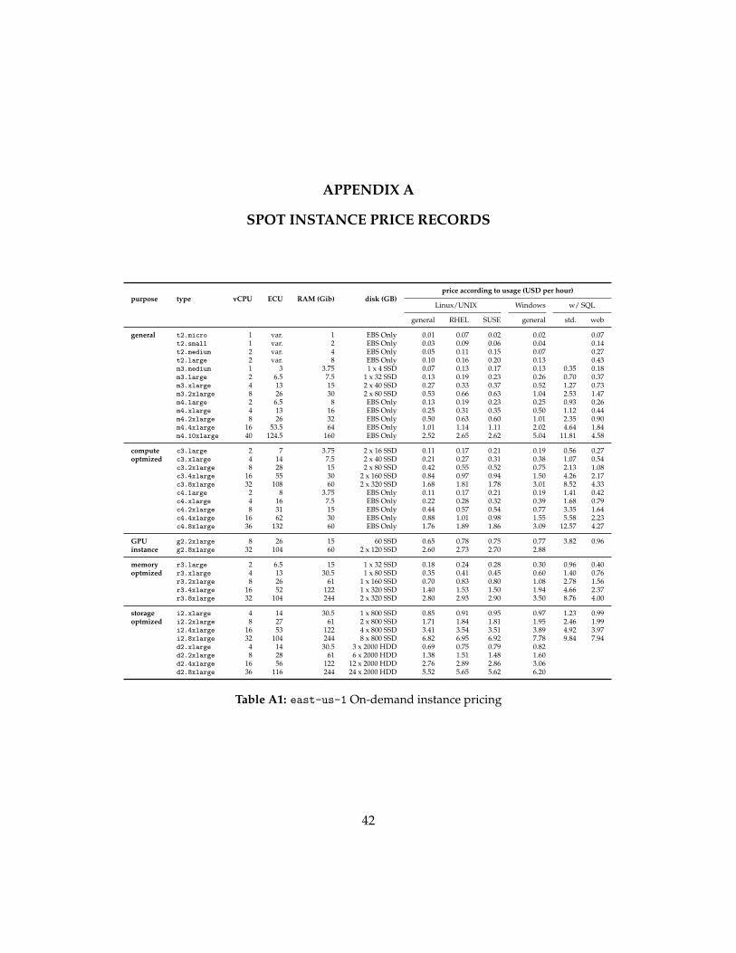
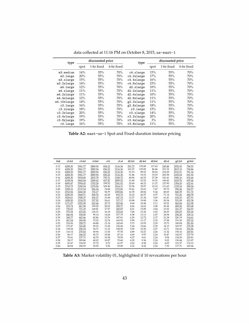
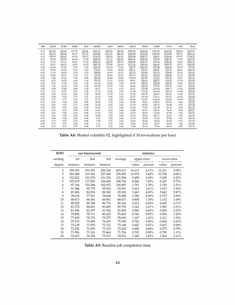
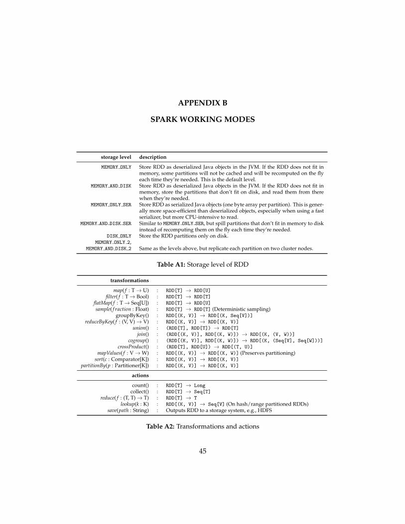
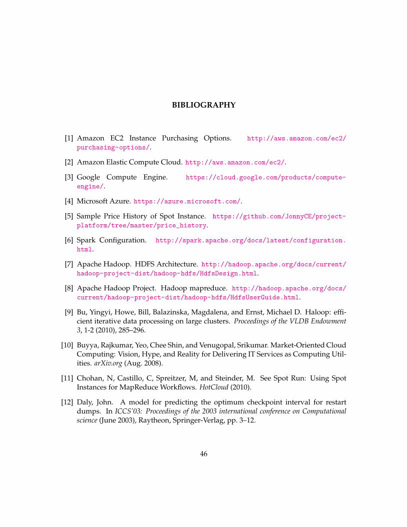
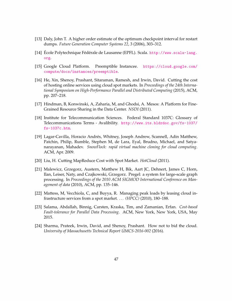
Related Documents