Analyzing friction forces with the Jarzynski equality

Analyzing friction forces with the Jarzynski equality

This article has been downloaded from IOPscience. Please scroll down to see the full text article.

2008 J. Phys.: Condens. Matter 20 354008

(http://iopscience.iop.org/0953-8984/20/35/354008)

Download details:

IP Address: 132.66.145.251

The article was downloaded on 12/08/2008 at 08:15

Please note that terms and conditions apply.

The Table of Contents and more related content is available

HOME | SEARCH | PACS & MSC | JOURNALS | ABOUT | CONTACT US

IOP PUBLISHING JOURNAL OF PHYSICS: CONDENSED MATTER

J. Phys.: Condens. Matter 20 (2008) 354008 (7pp) doi:10.1088/0953-8984/20/35/354008

Analyzing friction forces with theJarzynski equalityRonen Berkovich, Joseph Klafter and Michael Urbakh

School of Chemistry, Tel Aviv University, 69978 Tel Aviv, Israel

Received 4 March 2008, in final form 18 April 2008Published 11 August 2008Online at stacks.iop.org/JPhysCM/20/354008

AbstractWe investigate the applicability of the Jarzynski equality for reconstructing the energylandscape from force measurements obtained in single molecular unbinding and frictionexperiments. We demonstrate that single-well molecular potentials, such as the Lennard-Jonespotential, could be accurately recovered using a reasonable number of force traces (∼100)obtained for velocities which are experimentally accessible, v ≈ 5–100 nm s−1. The situationbecomes more complex in the presence of potential barriers in the energy profile. These includethe double-well and periodic potentials that we consider here. The slow convergence of thereconstruction procedure results from a large energy dissipation which occurs during jumpsacross the potential barriers. We suggest a modification of the reconstruction procedure whichallows the recovering of the correct shape of the potential wells even in the presence of potentialbarriers. However, a reconstruction of the potential shape in the vicinity of potential maximarequires additional information.

(Some figures in this article are in colour only in the electronic version)

1. Introduction

Experiments that probe mechanical forces on small scalesprovide a versatile tool for studying molecular adhesion andfriction through the response to the mechanical stress of singlemolecules or of nanoscale tips. The probing techniques includeatomic force microscopy (AFM) [1, 2], biomembrane forceprobe microscopy [3] and optical tweezers [4, 5]. Examplesof processes that are investigated are the specific binding ofligand-receptor [6, 7], protein unfolding [8, 9], the mechanicalproperties of single polymer molecules such as RNA [10, 11]and friction on the atomic scale [1, 2]. In these experiments,one probes forces along a reaction coordinate. One of the mainobjectives of the force measurements is to get information onthe free-energy landscape of the system under investigation.In friction force measurements this aim is usually approachedby comparing the force time series measured in the stick–slip regime of motion with the results of calculations withinTomlinson-like models [12–14], which provides an estimationof the amplitude of surface potential corrugation. However,this procedure is not unique and it does not give detailedinformation on the surface potential. Additional complicationsarise from the fact that the results of calculations depend on thevalue of the viscous dissipation constant entering the model,which is also unknown.

Recently, another approach for determining an energylandscape from force measurements has attracted a lot ofattention, mainly within the framework of single-molecularforce measurements [5, 15–18]. In these experiments, onemeasures the spring force, F , versus time or extension, andunbinding and rebinding events can be identified by the kinksin the corresponding force traces. A way to relate the free-energy difference between two thermodynamic states, �G, tothe work, wt , performed in converting one state to another isthrough the Jarzynski equality (JE) [15],

e−β�G(z) = 〈e−βwt 〉 (1)

where β = 1/kT , k is Boltzmann’s constant, T is theabsolute temperature and 〈· · ·〉 denotes the ensemble’s average.The equality allows us to extract equilibrium informationfrom nonequilibrium measurements—getting static internalinformation on the system from its dynamics. The accumulatedwork can be found as a path integral of the measured orcalculated force over the reaction coordinate. JE has beenapplied to reconstruct the free energy of a pulled substancefrom experimentally measured [5, 8, 18] and numericallysimulated [17, 19–23] force traces, in single molecular forcespectroscopy.

However, so far this approach was not applied to theinterpretation of friction force measurements. In this work we

0953-8984/08/354008+07$30.00 © 2008 IOP Publishing Ltd Printed in the UK1

J. Phys.: Condens. Matter 20 (2008) 354008 R Berkovich et al

demonstrate that the use of JE allows us to reconstruct a surfaceenergy profile defined by a periodic potential from the timeseries of frictional forces.

2. Jarzynski’s equality

JE deals with free-energy differences between states describedby different values of the coupling parameter λ. In the contextof force experiments, it gives the free energy of the entiresystem at different times. However, the position of the pullingmolecule, or tip, fluctuates, and as a result this is not thesame as the variation of the free energy along the pullingcoordinate, which we are seeking. This problem has beenresolved by Szabo and Hummer, who presented the JE in themore applicable form [17]:

G0(z) = − 1

βln

[∑t (

〈δ(z−zt )e−βwt 〉〈e−βwt 〉 )∑

t ( e−βV (z,t)

〈e−βwt 〉 )

](2)

where V (z, t) = ks/2(z(t) − λ(t))2 is the harmonic potentialdescribing the interaction with the pulling device, ks is theeffective elastic constant of the pulling device (for instance, ofthe AFM cantilever) and λ(t) = vt is the position of the AFMsupport or of the bead, whichs move with a constant velocity v.

Integrating equation (2) over z gives the Jarzynski equalityin equation (1). When putting JE into practice, it is importantto emphasize several aspects of this equality that have to betaken into account. The main quantity that JE uses is theaveraged weighted work 〈e−βwt 〉 rather than the work itself.This presents a major difficulty in the practical use of JE, sincethe exponential average in equation (2) is dominated by therare events which correspond to small values of the work andemerge from the work probability distribution’s tails. For thisreason the sampling of those trajectories that hold these rareevents is very meaningful [21, 24, 25]. Below, we examinethe sampling problem by discussing the required number ofrealizations for a reasonable convergence of the free energy.Another issue that should be addressed is the dependence of therequired number of realizations on the pulling velocity. Due tothe sampling problems, the further away our system gets fromequilibrium, there will be a price to pay, which is expressed inthe statistics.

3. Langevin equation (LE)

In order to illustrate the procedure for reconstruction of thefree energy, we generate force time series from the Langevinsimulations of single-molecular unbinding and friction. Thenthe accumulated work can be calculated by a simple integrationof the force trajectories:

wt = −∫

F(t) dλ = −∫

F(t)v dt . (3)

We start from the one-dimensional Langevin equation ofmotion for a particle of mass m:

md2z(t)

dt2= −ς

dz(t)

dt+ �(t) − ∂U(z, t)

∂z. (4)

Here z(t) is the particle position, U(z, t) is the potentialexperienced by the particle, ς is the microscopic frictioncoefficient, which is related to the diffusion coefficient D byς = kT

D , and �(t) is a fluctuating random force which ischaracterized by 〈�(t)〉 = 0 and satisfies the fluctuation-dissipation relation 〈�(t)�(t ′)〉 = 2ςkT δ(t − t ′), where δ(t)is the Dirac delta function. Due to the stochastic nature of LEwe obtain a large number of different trajectories for any giveninitial condition.

In the case of nanoscale systems considered here, theeffect of inertia on the dynamics is usually negligible, and thefull Langevin description in equation (4) can be reduced to theover-damped one given by the following equation:

dz(t)

dt= −β D

(�(t) − ∂U(z, t)

∂z

). (5)

In the calculations presented below, we limit ourselves to thisequation.

The total potential experienced by the pulled molecule ortip, U(z), includes two contributions: the inherent potentialof the system under study, (z), and the potential describingthe interaction with the pulling device, V (z, t). In the caseof unbinding or unfolding of single molecules the potential(z) defines the potential energy landscape of the molecule,while in the framework of friction (z) is a periodic potentialwhich describes an interaction between the driven tip and thesubstrate. The force measured in the unbinding and frictionexperiments is given by

F(t) = −ks(z(t) − vt). (6)

4. Lennard-Jones potential

In order to demonstrate how the JE works, we start from thecase of the rupture of molecular bonds. Here the potential (z)that is chosen is the Lennard-Jones potential

LJ(z) = U0

[(σ

z

)12

− 2

(σ

z

)6](7)

where U0 is the depth of the potential well and σ is the positionof the potential minima. Figure 1 presents an example of theforce time series obtained from a numerical solution of theLangevin equation (5) with the potential in (7).

The rupture force is quantified by the maximum extensionof the spring, which is followed by rapid recoil to its restposition. This behavior resembles the stick-to-slip transitionin studies on friction [1, 2]. Rupture of the molecular bondsoccurs by means of thermally assisted escape from the boundstate across an activation barrier. The latter diminishes asthe applied force increases, so the rupture force is determinedby interplay between the rate of escape in the absence of theexternal force and the pulling velocity (loading rate) [26, 27].Thus, the measured forces are not an intrinsic property of thebound complex, but rather depend on the mechanical setup andloading rate applied to the system.

In order to extract the molecular information fromthe force measurements we collected a number of force

2

J. Phys.: Condens. Matter 20 (2008) 354008 R Berkovich et al

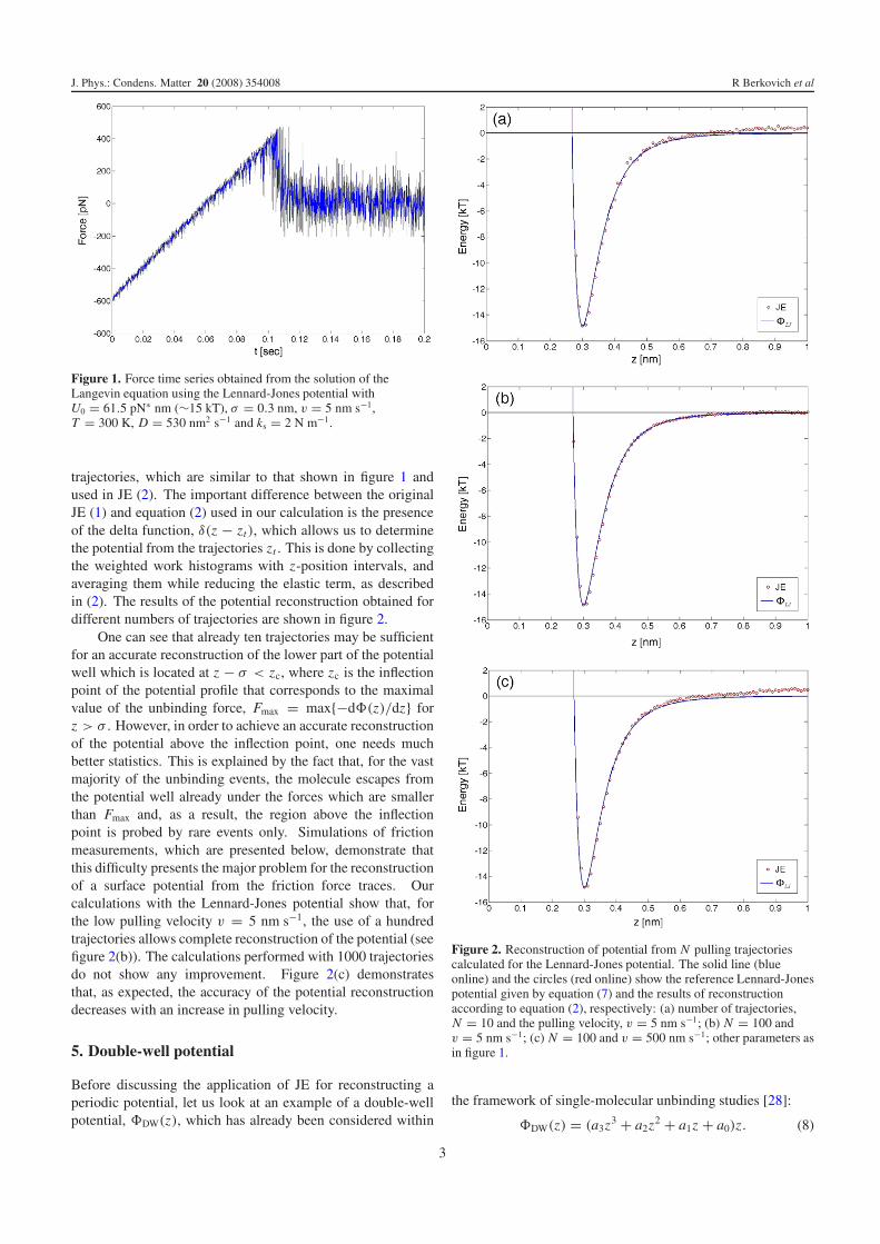
Figure 1. Force time series obtained from the solution of theLangevin equation using the Lennard-Jones potential withU0 = 61.5 pN∗ nm (∼15 kT), σ = 0.3 nm, v = 5 nm s−1,T = 300 K, D = 530 nm2 s−1 and ks = 2 N m−1.

trajectories, which are similar to that shown in figure 1 andused in JE (2). The important difference between the originalJE (1) and equation (2) used in our calculation is the presenceof the delta function, δ(z − zt), which allows us to determinethe potential from the trajectories zt . This is done by collectingthe weighted work histograms with z-position intervals, andaveraging them while reducing the elastic term, as describedin (2). The results of the potential reconstruction obtained fordifferent numbers of trajectories are shown in figure 2.

One can see that already ten trajectories may be sufficientfor an accurate reconstruction of the lower part of the potentialwell which is located at z − σ < zc, where zc is the inflectionpoint of the potential profile that corresponds to the maximalvalue of the unbinding force, Fmax = max{−d(z)/dz} forz > σ . However, in order to achieve an accurate reconstructionof the potential above the inflection point, one needs muchbetter statistics. This is explained by the fact that, for the vastmajority of the unbinding events, the molecule escapes fromthe potential well already under the forces which are smallerthan Fmax and, as a result, the region above the inflectionpoint is probed by rare events only. Simulations of frictionmeasurements, which are presented below, demonstrate thatthis difficulty presents the major problem for the reconstructionof a surface potential from the friction force traces. Ourcalculations with the Lennard-Jones potential show that, forthe low pulling velocity v = 5 nm s−1, the use of a hundredtrajectories allows complete reconstruction of the potential (seefigure 2(b)). The calculations performed with 1000 trajectoriesdo not show any improvement. Figure 2(c) demonstratesthat, as expected, the accuracy of the potential reconstructiondecreases with an increase in pulling velocity.

5. Double-well potential

Before discussing the application of JE for reconstructing aperiodic potential, let us look at an example of a double-wellpotential, DW(z), which has already been considered within

Figure 2. Reconstruction of potential from N pulling trajectoriescalculated for the Lennard-Jones potential. The solid line (blueonline) and the circles (red online) show the reference Lennard-Jonespotential given by equation (7) and the results of reconstructionaccording to equation (2), respectively: (a) number of trajectories,N = 10 and the pulling velocity, v = 5 nm s−1; (b) N = 100 andv = 5 nm s−1; (c) N = 100 and v = 500 nm s−1; other parameters asin figure 1.

the framework of single-molecular unbinding studies [28]:

DW(z) = (a3z3 + a2z2 + a1z + a0)z. (8)

3

J. Phys.: Condens. Matter 20 (2008) 354008 R Berkovich et al

Figure 3. Reconstruction of the double-well potential from 100pulling trajectories. The solid line (blue online), circles (red online)and triangles (black online) show the reference potential given byequation (8) and the results of reconstruction according toequation (2) obtained for two pulling velocities, v = 4 nm s−1 and0.4 nm s−1, respectively: (a) 1

DW(z) = (5z3 − 9z2 + 3)z, whichgives a barrier height of ∼7 kT, and the energy of the second well’sminima of ∼6 kT; (b) 2

DW(z) = (12z3 − 25z2 + 1)z which gives abarrier height of ∼15 kT, and the energy of the second well’s minimaof ∼2 kT. The spring constant, ks was taken as 15 pN nm−1 and thediffusion coefficient, D, was taken as 1 nm2 s−1. Energies are inunits of kT.

Here, contrary to the Lennard-Jones potential, there is abarrier separating two potential wells characteristic also of aperiodic potential. We have performed calculations for twodouble-well potentials, 1

DW and 2DW, with the corresponding

parameters: (i) a3 = 5 kT nm−4, a2 = −9 kT nm−3, a1 =0, a0 = 3 kT nm−1, and (ii) a3 = 12 kT nm−4, a2 =−25 kT nm−3, a1 = 0, a0 = 1 kT nm−1. These correspondto low and moderate potential barriers (see figure 3). Figure 3shows the results of applying JE (2) for a reconstruction ofthe double-well potential obtained for two different pullingvelocities.

A comparison of the results presented in figure 3 withthose obtained for the Lennard-Jones potential (see figure 2)leads to the following conclusions: (i) in order to recover

Figure 4. PDFs of the work dissipated during forward and backwardcycles for double-well potentials with low and moderate barriers:1

DW(z) = (5z3 − 9z2 + 3)z and 2DW(z) = (12z3 − 25z2 + 1)z,

respectively. The presented results correspond to two pullingvelocities, v = 4 nm s−1 and 0.4 nm s−1. Energies are in units of kT.Other parameters are as in figure 3.

a potential profile which includes a barrier, one has to usesignificantly lower pulling velocities than in the case ofa single-well potential; (ii) for moderate pulling velocitiesthe presence of the barrier leads to an increased error inthe reconstructed potential as one drives the system furtheraway from its original equilibrium state; and (iii) the errorgrows with the height of the barrier separating the twowells. The slow convergence of the reconstruction procedureoriginates from strong energy dissipation during jumps acrossthe potential barrier [25]. The energy dissipation reduces onlyslowly with a decrease in the pulling velocity; as a result, evenfor low velocities the system is far from the equilibrium.

Figure 4 shows the probability distribution functions(pdfs) for the energy dissipated during unbinding–rebindingcycles, Wd, which have been calculated for two kind of thedouble-well potentials discussed above. We see that for bothpotentials the most probable dissipated energy and the widthof pdfs reduce with a decrease of the pulling velocity. Inthe case of the moderate potential barrier of 15 kT evenfor a very low pulling velocity, v = 0.4 nm s−1, the mostprobable dissipated energy is of the order of 30 kT, indicatingthat the force ‘measurements’ are performed far from theequilibrium. This is different from the system with the lowbarrier (∼7 kT), where for v = 0.4 nm s−1 the most probabledissipated energy becomes as small as 3 kT. As a resultthe reconstruction procedure is successfully employed for thelow potential barrier and requires a very large number oftrajectories for the moderate barrier height.

6. Periodic potential

Let us look at experiments where the tip of the friction forcemicroscope (FFM) is dragged along a substrate surface, andthe measured lateral force exhibits stick–slip motion, as shownin figure 5. In this case, force traces include many unbinding

4

J. Phys.: Condens. Matter 20 (2008) 354008 R Berkovich et al

Figure 5. Force time series calculated for the periodic potential givenby equation (2). The inset shows the corresponding tip displacementversus time, as obtained by the solution of equation (5) with theperiodic potential in equation (9) with g = 0.3 nm, and the rest of theparameters are as used earlier in figure 1.

kinks. The results presented in this figure show one of the forcetraces obtained from the solution of the Langevin equation (5)with the symmetric periodic potential

PS(z) = −U0 cos

(2πz

g

)(9)

where U0 is the amplitude of the potential corrugation and gis the lattice constant. Stick–slip motion is observed when thepulling spring constant is weaker than the effective stiffness ofthe surface potential, max{′′(x)}. Usually, this condition iswritten in terms of the Tomlinson parameter, η [29],

η = (2π)2U0

ksg2> 1 (10)

which in our case equals η = 6.74.A direct application of JE (2) to the reconstruction of a

potential with a number of barriers, as in the case of a periodicpotential, is not quite practical, since it requires a very largenumber of force traces. As we have already noted above, theslow convergence of the reconstruction procedure originatesfrom strong energy dissipation during slip events when the tipcrosses the potential barriers [25, 28]. In order to improvethe convergence of reconstructing the potential, we dividedthe force time series into time segments corresponding to thelocations of the tip in the wells along the surface potential.The boundaries between the segments, which are shown bydashed lines in figure 5, have been chosen at those time pointswhere the absolute values of the force derivative are maximal.These points correspond to the jumps (slips) of the tip to thenext potential well. Each time segment was treated separately,setting the work accumulated at the previous segment to zero.The surface potential was then obtained using the JE (2) in thesame way as described above for the Lennard-Jones potential.Small uncertainties in the determination of the boundaries,which may arise from the limited experimental resolution, do

Figure 6. Reconstruction of the symmetric periodic potential from aset of 100 trajectories calculated for the pulling velocitiesv = 5 nm s−1 (a) and 500 nm s−1 (b). The solid line (blue online)and shows the reference periodic potential given by equation (9). Thecircles (red online) correspond to the reconstructed potential afterfiltering as discussed in the text. Other parameters are as in figure 1.

not influence the results. The proposed procedure is justifiedfor relatively low pulling velocities when, after each slip event,the tip approaches the equilibrium state before being pulled outof the well. This means that the rate of relaxation, (2π)2U0

g2η,

should be higher than the washboard frequency v/g. Forthe parameters used here this condition is valid for v <

1200 nm s−1. For an ideal surface it is enough to reconstructa potential with one well of the lattice. In order to do this,one needs only one segment of the stick–slip traces. However,in reality there might be defects present at the surface and,in order to identify them and their accurate location and tocharacterize their potential, we have to analyze a number ofstick–slip events.

Figure 6 shows the results of the potential reconstructionobtained from 100 force time series which have been calculatedfor two pulling velocities, v = 5 and 500 nm s−1. As inthe case of the Lennard-Jones potential, the lower part of theperiodic potential (below inflection points) is well reproducedfor both velocities. Due to very fast slips of the tip over the

5

J. Phys.: Condens. Matter 20 (2008) 354008 R Berkovich et al

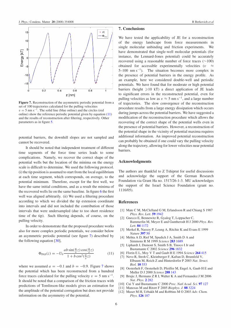
Figure 7. Reconstruction of the asymmetric periodic potential from aset of 100 trajectories calculated for the pulling velocitiesv = 5 nm s−1. The solid line (blue online) and the circles (redonline) show the reference periodic potential given by equation (11)and the results of reconstruction after filtering, respectively. Otherparameters as in figure 5.

potential barriers, the downhill slopes are not sampled andcannot be recovered.

It should be noted that independent treatment of differenttime segments of the force time series leads to somecomplications. Namely, we recover the correct shape of thepotential wells but the location of the minima on the energyscale is difficult to determine. We used the following protocol.(i) the tip position is assumed to start from the local equilibriumat each time segment, which corresponds, on average, to thepotential minimum. Therefore, except for the first well, wehave the same initial conditions, and as a result the minima ofthe recovered wells lie on the same baseline. In figure 6 the firstwell was aligned arbitrarily. (ii) We used a filtering procedureaccording to which we divided the tip extension coordinateinto intervals and did not included the contribution of thoseintervals that were undersampled (due to too short residencetime of the tip). Such filtering depends, of course, on thepulling velocity.

In order to demonstrate that the proposed procedure worksalso for more complex periodic potentials, we consider belowan asymmetric periodic potential (see figure 7) described bythe following equation [30],

PAS(z) = −U0

ab sin( πg z) cos( π

g z)

1 + b cos2( πg z)

(11)

where we assumed a = −0.1 and b = −0.9. Figure 7 showsthe potential which has been reconstructed from a hundredforce traces calculated for the pulling velocity v = 5 nm s−1.It should be noted that a comparison of the friction traces withpredictions of Tomlinson-like models gives an estimation forthe amplitude of the potential corrugation but does not provideinformation on the asymmetry of the potential.

7. Conclusions

We have tested the applicability of JE for a reconstructionof the energy landscape from force measurements insingle molecular unbinding and friction experiments. Wehave demonstrated that single-well molecular potentials (forinstance, the Lennard-Jones potential) could be accuratelyrecovered using a reasonable number of force traces (∼100)obtained for accessible experimentally velocities (v ≈5–100 nm s−1). The situation becomes more complex inthe presence of potential barriers in the energy profile. Asan example, here we considered double-well and periodicpotentials. We have found that for moderate or high potentialbarriers (height �10 kT) a direct application of JE leadsto significant errors in the reconstructed potential, even forpulling velocities as low as v ≈ 5 nm s−1, and a large numberof trajectories. The slow convergence of the reconstructionprocedure results from a large energy dissipation which occursduring jumps across the potential barriers. We have suggested amodification of the reconstruction procedure which allows therecovering of the correct shape of the potential wells even inthe presence of potential barriers. However, a reconstruction ofthe potential shape in the vicinity of potential maxima requiresadditional information. An improved potential reconstructioncan probably be obtained if one could vary the pulling velocityalong the trajectory, allowing for lower velocities near potentialbarriers.

Acknowledgments

The authors are thankful to Z Tshiprut for useful discussionsand acknowledge the support of the German ResearchFoundation via Grant Ha no. 1517/26-1-3. MU acknowledgesthe support of the Israel Science Foundation (grant no.1116/05).

References

[1] Mate C M, McClelland G M, Erlandsson R and Chiang S 1987Phys. Rev. Lett. 59 1942

[2] Gnecco E, Bennewitz R, Gyalog T, Loppacher C,Bammerlin M, Meyer E and Guntherodt H J 2000 Phys. Rev.Lett. 84 1172

[3] Merkel R, Nassoy P, Leung A, Ritchie K and Evans E 1999Nature 397 50

[4] Mehta A D, Rief M, Spudich J A, Smith D A andSimmons R M 1999 Science 283 1689

[5] Liphardt J, Dumont S, Smith S B, Tinoco I Jr andBustamante C 2002 Science 296 1832

[6] Florin E L, Moy V T and Gaub H E 1994 Science 264 415[7] Nevo R, Stroh C, Kleinberger F, Kaftan D, Brumfeld V,

Elbaum M, Reich Z and Hinterdorfer P 2003 Nat. Struct.Biol. 10 553

[8] Oesterhelt F, Oesterhelt D, Pfeiffer M, Engel A, Gaub H E andMuller D J 2000 Science 288 143

[9] Brujic J, Hermans Z R I, Walter K A and Fernandez J M 2006Nat. Phys. 2 282

[10] Cui Y and Bustamante C 2000 Proc. Natl Acad. Sci. 97 127[11] Manosas M and Ritort F 2005 Biophys. J. 88 3224[12] Muser M H, Urbakh M and Robbins M O 2003 Adv. Chem.

Phys. 126 187

6

J. Phys.: Condens. Matter 20 (2008) 354008 R Berkovich et al

[13] Dudko O K, Filippov A E, Klafter J and Urbakh M 2002Chem. Phys. Lett. 352 499

[14] Urbakh M, Klafter J, Gourdon D and Israelachvili J 2004Nature 430 525

[15] Jarzynski C 1997 Phys. Rev. Lett. 78 2690[16] Jarzynski C 1997 Phys. Rev. E 56 5018[17] Hummer G and Szabo A 2001 Proc. Natl Acad. Sci. 98 3658[18] Harris N C, Song Y and Kiang C H 2007 Phys. Rev. Lett.

99 068101[19] Kreuzer H J, Payne S H and Livadaru L 2001 Biophys. J.

80 2505[20] Braun O, Hanke A and Seifert U 2004 Phys. Rev. Lett.

93 158105

[21] Park S and Schulten K 2004 J. Chem. Phys. 120 5946[22] Minh D D L 2006 Phys. Rev. E 74 061120[23] Imparato A and Peliti L 2006 J. Stat. Mech. P03005[24] Hummer G 2001 J. Chem. Phys. 114 7330[25] Jarzynski C 2006 Phys. Rev. E 73 046105[26] Evans e 2001 Annu. Rev. Biophys. Biomol. Struct. 30 105[27] Dudko O K, Filippov A E, Klafter J and Urbakh M 2003 Proc.

Natl Acad. Sci. 100 11378[28] Adib A B and Minh D D L 2008 Phys. Rev. Lett. 100 180602[29] Socoliuc A, Bennewitz R, Gnecco E and Meyer E 2004 Phys.

Rev. Lett. 92 134301[30] Pesz K, Gabrys B J and Bartkiewicz S J 2002 Phys. Rev. E

66 061103

7