Analyzing Demand Data Presented By: Jonathan D. Washko, BS-EMSA Director of Deployment – REMSA President – Washko & Associates, LLC HPEMS & Public Safety.

Analyzing DemandData

Presented By:

Jonathan D. Washko, BS-EMSA

Director of Deployment – REMSAPresident – Washko & Associates, LLC

HPEMS & Public Safety Consulting Partner – Stout Solutions, LLC & FirstWatch

Analyzing Demand Data

• Discussion Topics– What is a Demand Analysis

– What kind of data do you need to calculate it

– What are some of the pitfalls to watch out for

– What formulas do you use to calculated it

– What tools do you use to calculate it

– What do you do with this information when completed


What is a Temporal Demand Analysis?

A Temporal Demand Analysis (or TDA) is an analysis of arrayed and aggregated historical call volume by week, hour of day and day of

week. It is used to help predict and determine the number of Quality Unit Hours needed (Demand) for each hour of the day and day of

week.

When completed, the analysis will provide staffing needs for a total of 168 hours (total number of hours in a week). From this analysis, a Peak Load Staffing Schedule can be built to match the prediction

model (Matching Supply with Demand).

Temporal Demand Analysis Fundamental Assumptions

– Assumes Each Call Takes one hour to complete (1:1 S/D Ratio)– Needs to be adjusted to each system accordingly– Use Task Time to adjust as needed if average is >< 60 minutes– Systems with lower Task Times require less resources– Systems with higher Task Times require more resources– Adjustments can be made through demand multipliers or the performing

of a Task Time TDA (A much more complex analysis)

Efficiency Alert! Controlling your system’s Task Time can have a HUGE financial impact on your system staffing costs so long as controls are kept to balance the triad.

Pitfall Alert! Inaccurate Task Time calculations can substantially impact the outcome of a demand analysis and put patient lives or an organization at risk. Perform the Task Time Analysis with due diligence and caution ensuring accuracy and validity!


Data Set Characteristics– Bad in / bad out concept– What to measure and why

• Requests, Responses or Transports?• Call Priorities to include or exclude• Standby / Special Events• Multi-Unit Responses• Other Variables (CCT, Specialized Units, Special Calls,

Special Circumstances, etc.)


Other Things You Need to Know– Desired response time reliability percentage– Inefficiency (LUH) buffer / cushion– Call volume seasonality– Some “Art” (SWAG)

• Response time requirements • Response time zone balancing requirements• Effects of city infrastructure (or lack there of)• Effects of traffic patterns• Effects of political “Posts”• Effects of other unique system anomalies


A Temporal Demand Analysis for Monday

Raw Demand Analysis Data.

P1, P2, P3, P4 & P7 Count of responses that arrived on scene by hour of day, day of week, chronologically ordered by date.

A total of 20 weeks worth of most recent data from the CAD system.





Military Date Format of Arrayed Days (Mondays) in Chronological OrderIn this case the date is Monday February 03, 2003





Hours of Day in Hour Ending Formate.g. 21 = 20:00 through 21:00





Total of All Hours for Each Week (Totaled Across)

In this case, there were 196 Responses on Feb. 10, 2003





Represents that on February 17, 2003 there

were 13 Responses between 11:00 and 12:00


A Temporal Demand Analysis for Mondays

Section II – EMS Production Model Art & Science, IV.c

Demand Analysis Analytics.

Used to calculate the required number of Quality Unit Hours (Demand) by Hour of day for this particular day of the week (In this case, Monday)

There are various statistical methods used to calculate system demand, all are accurate and correct. Experience has shown that Average Peak (a formula created by Jack Stout’s team) consistently yields an accurate prediction of the 90th Percentile of demand.


Total Responses for the HourTotaled by column (hour)

In this case the total is 72 responses for 03:00 to 04:00

XL Formula = sum(CR:CR)


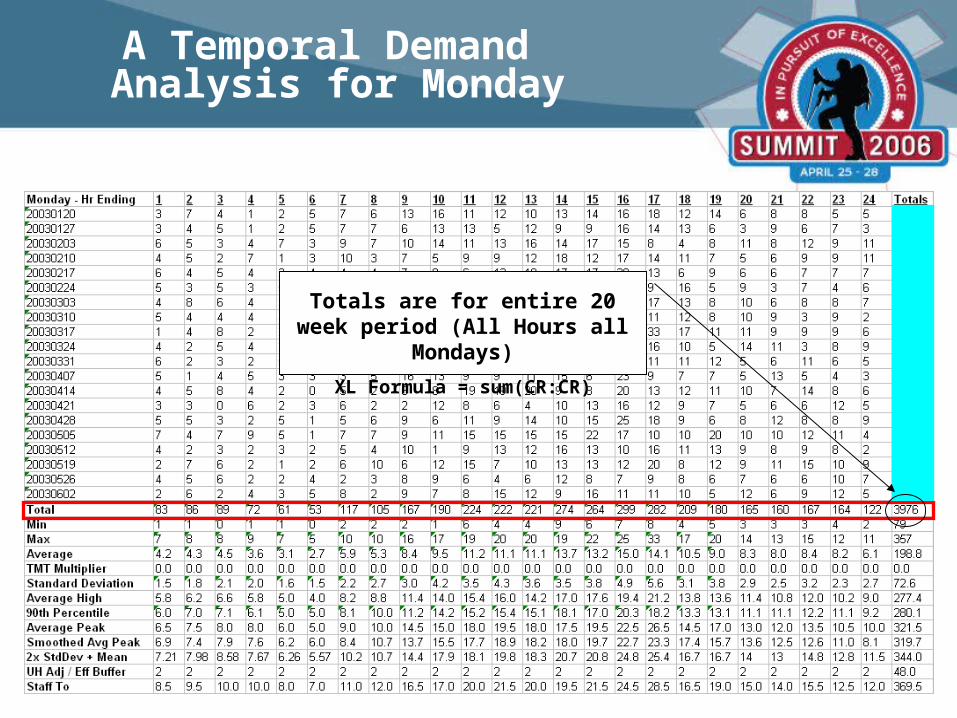
Totals are for entire 20 week period (All Hours all Mondays)



Min or Minimum number of Calls for the 20 week period for the hour of day and day of week.In this case the Min for 03:00 to 04:00 = 1

(Which occurs twice during the 20 week period)

XL Formula = min(CR:CR)


Total of Min or Minimum number of Calls by hour for all hours. Totaled by row (horizontally)

In this case the Total Min = 79



Max or Maximum number of Calls for the 20 week period for the hour of day and day of week.In this case the Max for 03:00 to 4:00 = 9

(Which occurs once during the 20 week period)

XL Formula = max(CR:CR)


Total of Max or Maximum number of Calls by hour for all hours. Totaled by row (horizontally)

In this case the Total Max = 357



Average number of Calls for the 20 week period for the hour of day and day of week.

In this case the Average for 03:00 to 4:00 = 3.6

XL Formula = average(CR:CR)


Total of Average number of Calls by hour for all hours. Totaled by row (horizontally) In this case the Total Average = 198.8



TMT (Total Mission Time) Multiplier is used to adjust demand calculations by taking the number and multiplying it times the Demand Measurement.

Example: if your Average TMT = 75 Minutes then Take 75 / 60 (minutes in an hour) = 1.25

This means that your Demand Measurement will be adjusted by 1.25 or 125%

In this case the TMT Multiplier = 0 for simplicity


Average of TMT Multiplier for all hours of this day. Totaled by row (horizontally)

In this case the Average = 0.0

XL Formula = Average(CR:CR)


The Standard Deviation of Responses for the hour. In this case the Standard Deviation for 03:00 to 04:00 = 2.0

XL Formula = stdev(CR:CR)


Total of Standard Deviation for all hours of this day. Totaled by row (horizontally)

In this case the total Standard Deviation = 72.6

XL Formula = Sum(CR:CR)


The Average High is a Stoutian Measurement that represents approximately the 75th percentile of

demand. It is calculated by taking the maximum number of calls in each consecutive 5 – 4 week periods

of a 20 week analysis then dividing the sum of these number by 5 (or average of the 5 periods)

In this example, the Average High for 03:00 to 04:00 = 5.8

The XL Formula: =(Max(CR:CR) + Max(CR:CR) + Max(CR:CR) + Max(CR:CR) + Max (CR:CR)) / 5The resultant is then multiplied by the TMT Multiplier for TMT Adjustments


Total of Average High for all hours of this day. Totaled by row (horizontally)

In this case the total Average High = 277.4



The 90th Percentile (or X Percentile) is a statistical ranking method used to determine the demand at X percent.

In this case the 90th Percentile Rank for 03:00 to 04:00 = 6.1

XL Formula = percentile(CR:CR,.9) where.9 = 90%The resultant is then multiplied by the TMT Multiplier for TMT Adjustments


Total of 90th Percentile for all hours of this day. Totaled by row (horizontally)

In this case the total 90th Percentile = 280.1



The Average Peak is a Stoutian Measurement that represents approximately the 90th percentile of

demand. It is calculated by taking the maximum number of calls in each consecutive 2 – 10 week

periods of a 20 week analysis then dividing the sum of these number by 2 (or average of the 2 periods)

In this example, the Average Peak for 03:00 to 04:00 = 8.0

The XL Formula: = (Max(CR:CR) + Max(CR:CR) ) / 2The resultant is then multiplied by the TMT Multiplier for TMT Adjustments


Total of Average Peak for all hours of this day. Totaled by row (horizontally)

In this case the total Average Peak = 321.5



The Smoothed Average Peak is a statistical smoothing of the Average Peak and is used to “blend” the severity

of hour to hour demand fluctuations for easier peak-load scheduling. It is calculated by taking 20% of the previous hour (Blue) + 60% of the current hour (Red) +

20% of the next hour (Yellow).

In this example, Smoothed Average Peak for 03:00 to 04:00 = 7.6

The XL Formula: = (CR*.2)+(CR*.6)+(CR*.2)


Total of Smoothed Average Peak for all hours of this day. Totaled by row (horizontally)

In this case the total Smoothed Average Peak = 319.7



2x StdDev + Mean is a Statistical Process Control methodology used by industry as an upper control chart limit. It represents approximately the 95% of

demand. It is calculated by taking the Standard Deviation (Red) calculated previously for the hour, multiplying it by 2 then adding it to the previously

calculated average (Blue).

In this example, 2x StdDev + Mean for 03:00 to 04:00 = 7.67

The XL Formula: = (CR*2)+(CR)The resultant is then multiplied by the TMT Multiplier for TMT Adjustments


Total of 2x StdDev + Mean for all hours of this day. Totaled by row (horizontally)

In this case the total 2x StdDev + Mean = 344.0



The UH Adj / Eff Buffer is used to allow managers the ability to adjust up or down their

staff to lines based on individual system needs. This is where some of the “art” comes in helping to determine this figure. This can also be used

to adjust the demand for contractual unit minimums and other needs.

In this case, the UH Adj / Eff Buffer for 03:00 to 04:00 = 2


Total of UH Adj / Eff Buffer for all hours of this day. Totaled by row (horizontally)

In this case the total UH Adj / Eff Buffer = 48.0



Adjusted Supply / Inefficiency Buffer

UH Adjustment Variables– The part of the “Art” of HPEMS (SWAG)– Response Time Requirements– Infrastructure Impacts– Geography / Coverage Area– System Idiosyncrasies and Their Impacts– Lost Unit Hours– Politics– Lots of Others


Demand Curve Adjustments

0.0

2.0

4.0

6.0

8.0

10.0

12.0

14.0

16.0

18.0

20.0

22.0

24.0

26.0

28.0

30.0

32.0

34.0

36.0

38.0

40.0

42.0

44.0

46.0

48.0

50.0

1 2 3 4 5 6 7 8 9 10 11 12 13 14 15 16 17 18 19 20 21 22 23 24

SAP Avg Peak Staff To Late Effective SUH

Example: Average Peak + 4 = Minimal Staffing

The Staff To line is the number of QUH required for that hour of that day. It typically defines the minimum number

of expected demand at X Percentile (Based on demand formula used). In this example, we are using the Average

Peak + UH Adj / Eff Buffer as our Staff to Calculation.The definition of this calculation varies by system and is not set. Frequently HPEMS systems use the Smoothed

Average Peak + UH Adj / Eff Buffer approach.

In this Example the Staff to Line for 03:00 to 04:00 = 10.0


Total of Staff to Line for all hours of this day. Totaled by row (horizontally)

In this case the Staff To Line = 369.5



So What Do All These Numbers Mean?


So What Do All These Numbers Mean?

• The Temporal Demand Analysis results in telling you how many Quality Unit Hours need to be produced by hour of day and day of week.

• Each hour of each day will have its own number for a total of 168 Production / Demand Requirements

• You build your “Production Schedule” to match these numbers


So What Do All These Numbers Mean?• The total columns come in handy as by adding the appropriate

total for each day will give you the total QUH requirement for the week.

• This number can then be used to calculate FTE’s, UHU and other budget figures.

• Keep in mind this is the optimal requirement. It is very difficult (if not near impossible) to create a schedule that exactly matches the demand requirements.

• The best Schedule to Demand matching I have experienced is +/- 2% to 3% variation.

• Zoll’s Resource Planner allows you to take Demand Data from this analysis to easily build a schedule that ACCURATELY matches your system’s Demand (see next session).


Tricks of the Trade…

• If your system is responsible for multiple geographic regions that are not contiguous or operate as separate deployment centers, a separate TDA for each area may be warranted

• Microsoft Excel or Microsoft Access (for advanced programmers) is the best tool for creating a TDA

• Microsoft Excel Pivot Tables allow for immediate arraying of data into tables that can then be copied and pasted into a TDA template


Tricks of the Trade…

You really only need a few key pieces of data to calculate the TDA raw data array

– TDA• Priority of the call• Call clock start date and time

– Hour of day and day of week calculations can be performed from this information

– GDA (plusTDA data)• Longitude of the call (or full address if not available)• Latitude of the call (or full address if not available)


Tools That Can Help…• FirstWatch

– FirstWatch (Data Surveillance Tool) has created a Demand Analysis Tool that allows for a “button push” assessment of demand that has an output file that can be directly imported into Zoll’s Resource Planner www.first-watch.us based on the templates used in this session.

• Zoll Data Systems / Washko & Associates– Working on developing a Resource Planner Add On that will

allow you to import demand data directly into Resorce Planner– Developed an exclusive arrangement for customers looking for

additional expertise and help (Speak with me or your Zoll Sales Representitive)


Questions / Discussion…


Analyzing Demand Data Presented By: Jonathan D. Washko, BS-EMSA Director of Deployment – REMSA President – Washko & Associates, LLC HPEMS & Public Safety.

Documents

demand data slide

raw demand analysis

task time analysis

demand multipliers

demand data discussion

analysis of arrayed

recent data

day of week